Embed Size (px)
Citation preview

VERSION 1.3.5 NIST UNCERTAINTY MACHINE
NIST Uncertainty Machine — User’s Manual
Thomas Lafarge Antonio Possolo
Statistical Engineering DivisionInformation Technology Laboratory
National Institute of Standards and TechnologyGaithersburg, Maryland, USA
March 10, 2018
1 NIST Uncertainty Machine for the Impatient
• Using a Web browser, visit https://uncertainty.nist.gov/.
• Choose the number of input quantities from the drop-down menu, andgive them names if desired.
• Select a probability distribution for each of the input quantities, and entervalues for its parameters (in the absence of cogent reason to do otherwise,assign Gaussian distributions to the input quantities, with means equal toestimates of their values, and standard deviations equal to their standarduncertainties);
• Specify the size of the Monte Carlo sample to be drawn from the proba-bility distribution of the output quantity (no larger than 5000 000).
• Enter one or more valid R expressions (one per line) into the box la-beled Value of output quantity (R expression) such that the lastline evaluates to f (x1, . . . , xn), the right-hand side of the measurementequation. (Refer to (U-8) on Page 11 for the case when the output quan-tity is a vector.)
• If there are correlations between the input quantities, then check the boxmarked Correlations, enter the values of the non-zero correlations, andselect a copula to apply them with (cf. Figure 6 on Page 26).
• Click the button labeled Run the computation.
LAFARGE & POSSOLO PAGE 1 OF 46
VERSION 1.3.5 NIST UNCERTAINTY MACHINE
2 Purpose
The NIST Uncertainty Machine (https://uncertainty.nist.gov/) is a Web-based software application to evaluate the measurement uncertainty associ-ated with an output quantity defined by a measurement model of the formy = f (x1, . . . , xn).
The function f must be specified fully and explicitly, either as a formula or asan algorithm that, given vectors of values of the inputs, all of the same length,produces a vector of values of the output, also of the same length as the inputs— this is the sense in which we say, throughout this manual, that f must be“vectorized.”
The input quantities are modeled as random variables whose joint probabilitydistribution also has to be fully specified. In many applications, f is real-valued(but vectorized as just mentioned). Section 12, beginning on Page 28, showshow the NIST Uncertainty Machinemay also be used to produce the elementsneeded for a Monte Carlo evaluation of uncertainty for a multivariate measur-and: that is, when, given a single set of scalar inputs x1, . . . , xn, y is a vector(whose length may be different from n). The example presented in section 12(Voltage Reflection Coefficient) illustrates this case.
Lafarge and Possolo [2015] describe an early version of the NIST Uncertainty
Machine and an important innovation implemented in it: the computation ofthe uncertainty budget based entirely on the results of the Monte Carlo method.Both Bell [1999] and Hall and White [2018] provide succinct, very accessibleintroductions to the concepts and basic techniques for the evaluation of mea-surement uncertainty. Possolo [2015] and Possolo and Iyer [2017] provide moreextensive introductions that include many illustrative examples drawn from thepractice of measurement science.
The NIST Uncertainty Machine evaluates measurement uncertainty by appli-cation of two different methods:
• The method introduced by Gauss [1823] and popularized by Kline andMcClintock [1953], particularly among the engineering and physics com-munities — this method is described succinctly by Taylor and Kuyatt [1994],and more detailedly in the Guide to the Evaluation of Uncertainty in Mea-surement (GUM) [Joint Committee for Guides in Metrology, 2008a];
• The Monte Carlo method described by Morgan and Henrion [1992] inthe context of measurement science, which is specified in Supplements 1(GUM-S1) and 2 (GUM-S2) to the GUM [Joint Committee for Guides in
LAFARGE & POSSOLO PAGE 2 OF 46
VERSION 1.3.5 NIST UNCERTAINTY MACHINE
Metrology, 2008b, 2011] — Possolo et al. [2009] dispel some commonmisunderstandings about the application of the techniques described inthe GUM-S1.
3 Gauss’s Formula vs. Monte Carlo Method
The method described in the GUM produces an approximation to the standardmeasurement uncertainty u(y) of the output quantity, starting from:
(a) Estimates x1, . . . , xn of the input quantities, which must be specified by theuser;
(b) Standard measurement uncertainties u(x1), . . . , u(xn) associated with theinput quantities, which also must be specified by the user;
(c) Correlations ri j between every pair of different input quantities, whichthe NIST Uncertainty Machine assumes all to be zero unless the user ex-plicitly specifies other values for them;
(d) Values of the partial derivatives of f evaluated at x1, . . . , xn, which the userneed not concern herself with, because the NIST Uncertainty Machine
does all the necessary calculations.
When the probability distribution of the output quantity is approximately Gaus-sian, then the interval y ± 2u(y) may be interpreted as a coverage interval forthe measurand with approximately 95 % coverage probability.
By a felicitous coincidence this also holds for some markedly non-Gaussian prob-ability distributions, including many instances of the Student’s t, lognormal,gamma, and Weibull distributions [Freedman et al., 2007].
However, and in general, the probabilistic meaning of other intervals, for ex-ample y±u(y) or y±3u(y), typically will be markedly dependent on the prob-ability distribution assigned to y . For example, if this distribution is Gaussian,then y ±u(y) has coverage probability 68 %, but 76 % when the distribution isLaplace (or double exponential).
The GUM also considers the case where the distribution of the output quantityy is approximately Student’s t with a number of degrees of freedom that is afunction of the numbers of degrees of freedom that the u(x j) are based on,computed using the Welch-Satterthwaite formula [Satterthwaite, 1946, Welch,1947].
LAFARGE & POSSOLO PAGE 3 OF 46
VERSION 1.3.5 NIST UNCERTAINTY MACHINE
In general, neither the Gaussian nor the Student’s t distributions need modelthe dispersion of values of the output quantity accurately, even when all theinput quantities are adequately modeled as Gaussian random variables.
The GUM suggests that the Central Limit Theorem (CLT) from Probability The-ory [DeGroot and Schervish, 2011] lends support to the Gaussian approxima-tion for the distribution of the output quantity. However, without a detailedexamination of the measurement function f , and of the probability distributionof the input quantities (examinations that the GUM does not explain how todo), it is impossible to guarantee the adequacy of the Gaussian or Student’s tapproximations.
NOTE. The CLT states that, under specified conditions, a sum of indepen-dent random variables has a probability distribution that is approximatelyGaussian [Billingsley, 1979, Theorem 27.2]. The CLT is a limit theorem,in the sense that it concerns an infinite sequence of sums, and providesno indication about how close to Gaussian the distribution of a sum witha finite number of summands will be. Other results in probability theoryprovide such indications, but they involve more than just the means andvariances that are required to apply Gauss’s formula [Friedrich, 1989].NOTE. The reason why the CLT may be relevant is the following: if thefunction f is sufficiently smooth in a neighborhood of the point (in n-dimensional Euclidean space) (ξ1, . . . ,ξn), whose coordinates are the truevalues of the input quantities, then f (x1, . . . , xn)≈ f (ξ1, . . . ,ξn)+ f1(x1, . . . , xn)(x1−ξ1) + · · · + fn(x1, . . . , xn)(xn − ξn), where the fi denote the first-orderpartial derivatives of f . The right-hand side is a sum of random variableswhen the x i are modeled as random variables.
Application of the Monte Carlo method produces an arbitrarily large samplefrom the probability distribution of the output quantity, and it requires thatthe joint probability distribution of the random variables modeling the inputquantities be specified fully.
This sample alone suffices: (i) to compute the standard uncertainty associatedwith the output quantity; (ii) to compute and to interpret coverage intervalsprobabilistically; and (iii) to estimate the proportions of the squared uncertaintyu2(y) that are attributable to the sources of uncertainty corresponding to the thedifferent input quantities (the so-called uncertainty budget), using the techniquedescribed by Lafarge and Possolo [2015].
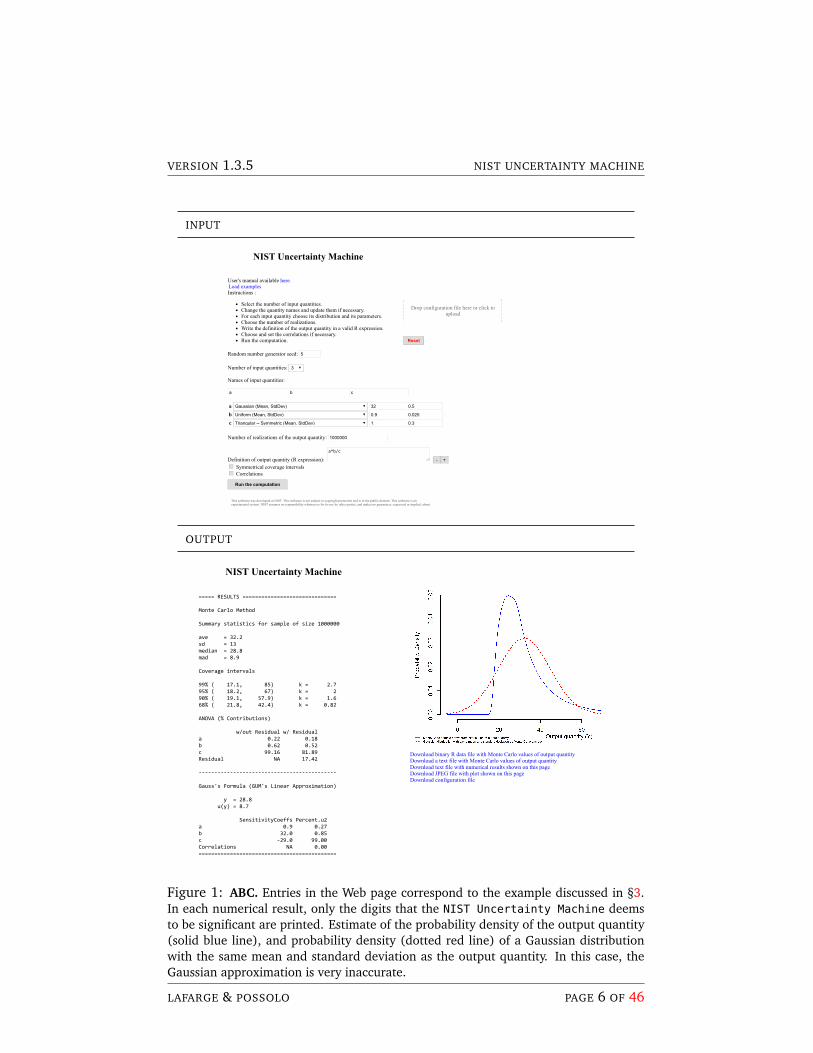
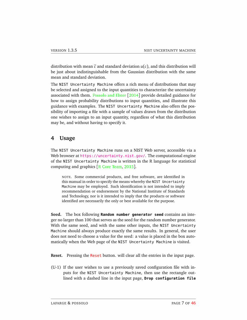
EXAMPLE. Suppose that the measurement model is y = ab/c, and that a,b, and c are modeled as independent random variables such that:
• a is Gaussian with mean 32 and standard deviation 0.5;
LAFARGE & POSSOLO PAGE 4 OF 46
VERSION 1.3.5 NIST UNCERTAINTY MACHINE
• b has a uniform (or, rectangular) distribution with mean 0.9 andstandard deviation 0.025;
• c has a symmetrical triangular distribution with mean 1 and stan-dard deviation 0.3.
Figure 1 on Page 6 shows the graphical user interface of the NIST UncertaintyMachine filled in to reflect these modeling choices, and the results that arereturned and displayed by the browser. To load the specifications for thisexample into the NIST Uncertainty Machine, click here.
The method described in the GUM produces y = 32.2 and u(y) = 12.5.According to the conventional interpretation, the interval y ± 2u(y) =(18,67.1) may be a coverage interval with approximately 95 % coverageprobability. (The results of the Monte Carlo method can be used to showthat the effective coverage of this interval is 95.5 %.)
Since the NIST Uncertainty Machine requires that the probability distribu-tion of the input quantities be specified, in the absence of cogent reason to dootherwise, the user may assign Gaussian (or, normal) distributions to them:
• If the input quantities are uncorrelated, then this amounts to assigninga Gaussian distribution to each one of them, with mean and standarddeviation equal to the corresponding estimate and standard uncertainty;
• If the input quantities are correlated, then besides assigning Gaussian dis-tributions to them as in the previous case, then the user will also need tocheck the box marked Correlation in the interface of the NIST Uncertainty
Machine, and then specify the values of the correlations, and select aGaussian copula (if indeed a multivariate Gaussian distribution is desired)to enforce the correlations [Possolo, 2010].
In many cases there is cogent reason to assign non-Gaussian distributions to atleast some of the input quantities.
For example, if the quantity takes values between known lower and upper limits,then a (shifted and re-scaled) beta distribution with suitably chosen parametersmay be an appropriate model: the uniform (or, rectangular) distribution is aspecial case of the beta distribution.
For another example, suppose that f (x1, . . . , xn) involves a ratio, as in the ex-ample above, where y = ab/c. Then c should not be assigned a normal distri-bution because the corresponding probability density is positive at 0, and y willhave infinite variance. If the true value of c is known to be positive, and bc is itsestimate, and u(c)/bc is less than 5 %, say, then c may be assigned a lognormal
LAFARGE & POSSOLO PAGE 5 OF 46
VERSION 1.3.5 NIST UNCERTAINTY MACHINE
INPUT
NIST Uncertainty Machine
User's manual available here.
Instructions :
Select the number of input quantities.Change the quantity names and update them if necessary.For each input quantity choose its distribution and its parameters.Choose the number of realizations.Write the definition of the output quantity in a valid R expression.Choose and set the correlations if necessary.Run the computation.
Drop configuration file here or click toupload
Reset
Random number generator seed: 5 Number of input quantities: 3
Names of input quantities:
a b c
a Gaussian (Mean, StdDev) 32 0.5
b Uniform (Mean, StdDev) 0.9 0.025
c Triangular -- Symmetric (Mean, StdDev) 1 0.3
Number of realizations of the output quantity: 1000000
Definition of output quantity (R expression): a*b/c
- + Symmetrical coverage intervals Correlations
Run the computation
This software was developed at NIST. This software is not subject to copyright protection and is in the public domain. This software is anexperimental system. NIST assumes no responsibility whatsoever for its use by other parties, and makes no guarantees, expressed or implied, about
Load examples
OUTPUT
===== RESULTS ============================== Monte Carlo Method Summary statistics for sample of size 1000000 ave = 32.2 sd = 13 median = 28.8 mad = 8.9 Coverage intervals 99% ( 17.1, 85) k = 2.7 95% ( 18.2, 67) k = 2 90% ( 19.1, 57.9) k = 1.6 68% ( 21.8, 42.4) k = 0.82 ANOVA (% Contributions) w/out Residual w/ Residual a 0.22 0.18 b 0.62 0.52 c 99.16 81.89 Residual NA 17.42 -------------------------------------------- Gauss's Formula (GUM's Linear Approximation) y = 28.8 u(y) = 8.7 SensitivityCoeffs Percent.u2 a 0.9 0.27 b 32.0 0.85 c -29.0 99.00 Correlations NA 0.00 ============================================
Download binary R data file with Monte Carlo values of output quantity Download a text file with Monte Carlo values of output quantity Download text file with numerical results shown on this page Download JPEG file with plot shown on this page Download configuration file
NIST Uncertainty Machine
Figure 1: ABC. Entries in the Web page correspond to the example discussed in §3.In each numerical result, only the digits that the NIST Uncertainty Machine deemsto be significant are printed. Estimate of the probability density of the output quantity(solid blue line), and probability density (dotted red line) of a Gaussian distributionwith the same mean and standard deviation as the output quantity. In this case, theGaussian approximation is very inaccurate.
LAFARGE & POSSOLO PAGE 6 OF 46
VERSION 1.3.5 NIST UNCERTAINTY MACHINE
distribution with mean bc and standard deviation u(c), and this distribution willbe just about indistinguishable from the Gaussian distribution with the samemean and standard deviation.
The NIST Uncertainty Machine offers a rich menu of distributions that maybe selected and assigned to the input quantities to characterize the uncertaintyassociated with them. Possolo and Elster [2014] provide detailed guidance forhow to assign probability distributions to input quantities, and illustrate thisguidance with examples. The NIST Uncertainty Machine also offers the pos-sibility of importing a file with a sample of values drawn from the distributionone wishes to assign to an input quantity, regardless of what this distributionmay be, and without having to specify it.
4 Usage
The NIST Uncertainty Machine runs on a NIST Web server, accessible via aWeb browser at https://uncertainty.nist.gov/. The computational engineof the NIST Uncertainty Machine is written in the R language for statisticalcomputing and graphics [R Core Team, 2015].
NOTE. Some commercial products, and free software, are identified inthis manual in order to specify the means whereby the NIST UncertaintyMachine may be employed. Such identification is not intended to implyrecommendation or endorsement by the National Institute of Standardsand Technology, nor is it intended to imply that the products or softwareidentified are necessarily the only or best available for the purpose.
Seed. The box following Random number generator seed contains an inte-ger no larger than 100 that serves as the seed for the random number generator.With the same seed, and with the same other inputs, the NIST Uncertainty
Machine should always produce exactly the same results. In general, the userdoes not need to choose a value for the seed: a value is placed in the box auto-matically when the Web page of the NIST Uncertainty Machine is visited.
Reset. Pressing the Reset button. will clear all the entries in the input page.
(U-1) If the user wishes to use a previously saved configuration file with in-puts for the NIST Uncertainty Machine, then use the rectangle out-lined with a dashed line in the input page, Drop configuration file
LAFARGE & POSSOLO PAGE 7 OF 46
VERSION 1.3.5 NIST UNCERTAINTY MACHINE
here or click to upload: either drag the file onto it, or click insidethis rectangle and then look for and select the file where the input pa-rameters will have been saved previously. (U-12) explains how to savea configuration file that may be used subsequently to re-run the samecomputation.
(U-2) Choose the number of input quantities from the drop-down menu cor-responding to the entry Number of input quantities. In response tothis, the Web page will update itself and show as many boxes as thereare input quantities, and assign default names to them (which may bechanged as explained next).
(U-3) Enter the names of the input quantities into the boxes following Names
of input quantities. The same names will automatically become thelabels of the rows of boxes that appear immediately below and that areused to specify probability distributions for the input quantities.
(U-4) Assign a probability distribution to each of the input quantities usingthe drop-down menus in front of them. A few commonly used distri-butions will be readily available. Clicking on More choices will revealothers. Once a choice is made, one or more additional input boxes willappear, where values of parameters must be entered fully to specify theprobability distribution that was selected. If the choice is Sample values
(between 30 and 100000), then a rectangle outlined with a dashed linewill appear in the same row, saying Drop sample file here or click
to upload.
Table 2 on Page 14 lists the distributions implemented currently, andtheir parametrizations. Note that some distributions can be parametrizedin any one of several different ways: in such cases, only one of theparametrizations needs to be specified. For example, specifying a rect-angular distribution whose left and right end-points are 0.37 and 0.41 isequivalent to specifying a rectangular distribution whose mean is (0.34+0.42)/2 = 0.38 and whose standard deviation is (0.42 − 0.34)/
p12 =
0.023.
The NIST Uncertainty Machine does not accept standard deviationsthat are set to 0 — however, this is detected only at run time (afterthe user will have pressed the button labeled Run the computation).Declaring the standard deviation to be 0 would be equivalent to speci-fying the value of a constant, which can be done either by entering thisvalue as a numerical constant in the expression that defines the output
LAFARGE & POSSOLO PAGE 8 OF 46
VERSION 1.3.5 NIST UNCERTAINTY MACHINE
quantity (cf. the example in Section 11 that begins on Page 25), or byselecting Constant as distribution type and entering the value of the con-stant in the corresponding box.
(U-5) As already mentioned above, the NIST Uncertainty Machine allowsthe user to provide a sample drawn from the probability distribution of aninput quantity instead of selecting a particular distribution from amongthose that the NIST Uncertainty Machine offers.
To provide such sample, select Sample values (between 30 and 100000)
from the drop-down menu with the list of distributions, and then use therectangle outlined with a dashed line that will have appeared in the in-put page, in front of the box corresponding to the input quantity, Dropsample file here or click to upload: either drag the file onto it,or click it and then look for and select the file containing the samplevalues.
The data file is then parsed and all the numbers present in it will beloaded. The numerical values may be arranged in the file in any waythat is convenient for the user — one or several per line —, but must beseparated from one another by any (not necessarily the same throughoutthe file) non-numeric character or string of non-numeric characters. Thenumbers may be written either in decimal or scientific notation, and inthis case using e or E to denote the appropriate power of ten. For exam-ple, 1983.76 may also be written either as 1.98376e3 or as 1.98376E3.Once the file has been parsed the number of values loaded will be shownto ensure that it matches the user’s expectation. The total number ofsample values provided in this way, summed across all input quantitiesfor which samples are provided, cannot exceed 2400 000 approximately.In case this limit is reached, an error message appears once the compu-tation starts.
The NIST Uncertainty Machine operates essentially in the same wayregardless of whether parametric distributions are specified, or samplesfrom otherwise unspecified distributions are provided. The main differ-ence is that, for the latter, the NIST Uncertainty Machine resamplesthe values in the sample that was provided repeatedly, uniformly at ran-dom with replacement (that is, all values in the sample provided areequally likely to be drawn, and all are available for drawing when a drawis made). §13 illustrates this feature, and provides additional informa-tion about it.
LAFARGE & POSSOLO PAGE 9 OF 46
VERSION 1.3.5 NIST UNCERTAINTY MACHINE
(U-6) Enter the size of the Monte Carlo sample to be drawn from the proba-bility distribution of the output quantity, into the box labeled Number of
realizations of the output quantity: the default value, 1× 10⁶, isthe minimum recommended sample size (currently the NIST Uncertainty
Machine is able to generate samples of size from 1× 10⁵ to 5× 10⁶).
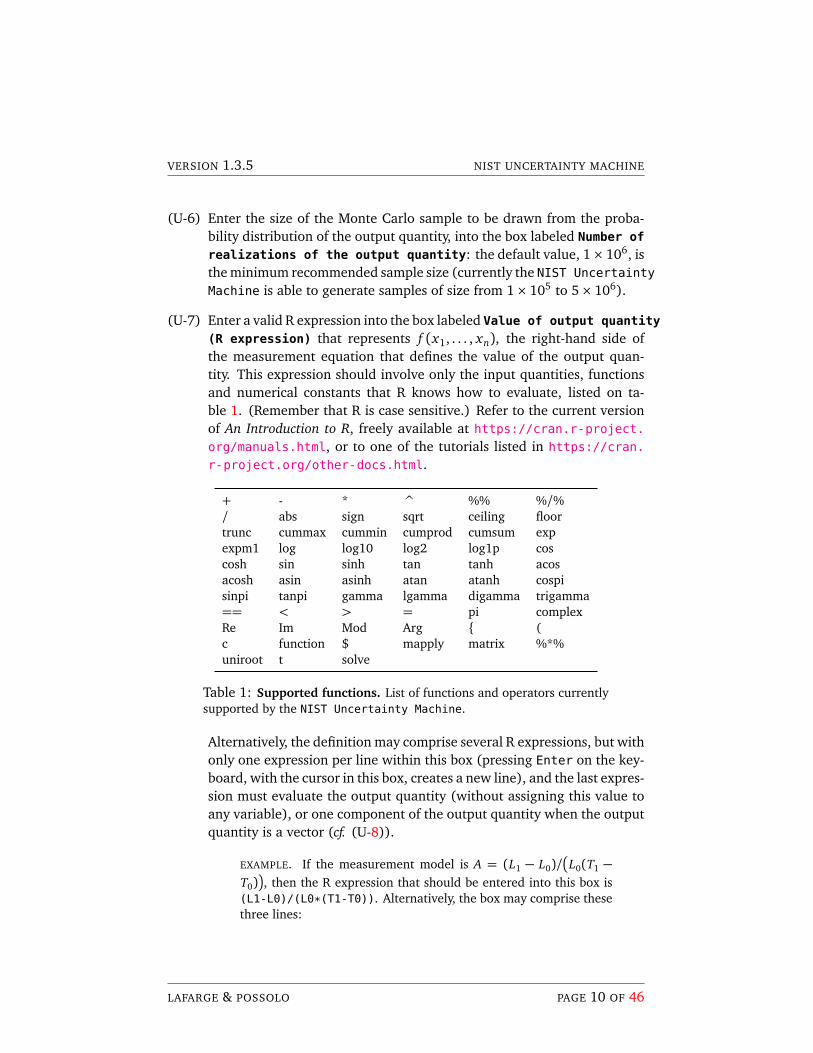
(U-7) Enter a valid R expression into the box labeled Value of output quantity
(R expression) that represents f (x1, . . . , xn), the right-hand side ofthe measurement equation that defines the value of the output quan-tity. This expression should involve only the input quantities, functionsand numerical constants that R knows how to evaluate, listed on ta-ble 1. (Remember that R is case sensitive.) Refer to the current versionof An Introduction to R, freely available at https://cran.r-project.org/manuals.html, or to one of the tutorials listed in https://cran.
r-project.org/other-docs.html.
+ - * ^ %% %/%/ abs sign sqrt ceiling floortrunc cummax cummin cumprod cumsum expexpm1 log log10 log2 log1p coscosh sin sinh tan tanh acosacosh asin asinh atan atanh cospisinpi tanpi gamma lgamma digamma trigamma== < > = pi complexRe Im Mod Arg (c function $ mapply matrix %*%uniroot t solve
Table 1: Supported functions. List of functions and operators currentlysupported by the NIST Uncertainty Machine.
Alternatively, the definition may comprise several R expressions, but withonly one expression per line within this box (pressing Enter on the key-board, with the cursor in this box, creates a new line), and the last expres-sion must evaluate the output quantity (without assigning this value toany variable), or one component of the output quantity when the outputquantity is a vector (cf. (U-8)).
EXAMPLE. If the measurement model is A = (L1 − L0)/
L0(T1 −T0)
, then the R expression that should be entered into this box is(L1-L0)/(L0*(T1-T0)). Alternatively, the box may comprise thesethree lines:
LAFARGE & POSSOLO PAGE 10 OF 46
VERSION 1.3.5 NIST UNCERTAINTY MACHINE
N = L1-L0D = L0*(T1-T0)N / D
The NIST Uncertainty Machine requires that the measurement func-tion f be vectorized: that is, if each of its arguments is a vector of lengthK , then the value of f , specified in the last line of the box, must be avector of length K such that the kth element of this vector is the valueof f at the kth values of all the input quantities. This may not happenautomatically for some intricate measurement equations that involve op-timizations, root-finding, or solutions of differential equations, amongothers. In the example described in §13, vectorization is achieved sim-ply by invoking the R function mapply, which applies the same functionto sets of corresponding values of its arguments.
NOTE. The NIST Uncertainty Machine may report Impossible toevaluate the output expression. This may be caused by the use of anR function that the NIST Uncertainty Machine does not recognizeyet. When such message is encountered, please send an eMail mes-sage to both [email protected] and [email protected],showing the inputs that induced such response.
(U-8) If the output quantity is a vector with p components, press the “+” buttonp−1 times to create a total of p output fields. Enter an R expression intoeach one of them similarly to how the specification of the value of theoutput quantity was described in (U-7).
(U-9) If symmetrical coverage intervals are desired, then check the box markedSymmetrical coverage intervals. These intervals take a little longerto compute than those computed by default (which may be asymmetri-cal), and are of the form by ± ku(y) where by , the estimate of the outputquantity, is the average of the Monte Carlo sample, and the coverage fac-tor k depends on the specified coverage probability.
NOTE. The default coverage interval with coverage probability 0 <γ < 1 is (y∗(1−γ)/2, y∗(1+γ)/2), whose endpoints are the 50(1 − γ)thand 50(1+ γ)th percentiles of the Monte Carlo sample drawn fromthe probability distribution of the output quantity. These need notbe equidistant from the average (or from the median) of the sam-ple. The corresponding coverage factor is computed as k = (y∗(1+γ)/2−y∗(1−γ)/2) /(2u(y)), and it is not particularly meaningful when theinterval is not symmetrical (that is, when it is not centered on theestimate of the output quantity).
LAFARGE & POSSOLO PAGE 11 OF 46
VERSION 1.3.5 NIST UNCERTAINTY MACHINE
Even for symmetrical intervals (those that are centered on the aver-age of the Monte Carlo sample drawn from the probability distribu-tion of the output quantity), the coverage factor k is computed onlyafter the coverage interval has been derived from this sample, hencedifferently from how it is computed in the GUM.
(U-10) If there are non-null correlations between input quantities that need tobe taken into account, then check the box marked Correlations, andenter the values of non-zero correlations into the appropriate boxes inthe upper triangle of the correlation matrix that the browser will display.
NOTE. Not all combinations of values of the correlations that may beentered produce a valid correlation matrix, which must be symmet-rical, have all entries between −1 and +1, and have only positiveeigenvalues. The NIST Uncertainty Machine issues an error mes-sage (Illegal correlation matrix) if these conditions are not allmet.
(U-11) If the box marked Correlations has been checked, then besides havingspecified correlations in (U-10), also select a copula (currently, eitherGaussian or Student’s t) to manufacture a joint probability distributionfor the input quantities. This is needed because there are infinitely manymultivariate distributions with the same means, standard deviations, andcorrelations [Nelsen, 2006]. If the copula chosen is (multivariate) Stu-dent’s t, then another box will appear nearby to receive the desired num-ber of degrees of freedom.
NOTE. The resulting joint distribution reproduces the correlationstructure that has been specified, and has the distributions specifiedfor the input quantities as margins. Possolo [2010] explains andillustrates the role that copulas play in uncertainty analysis.
(U-12) Click the button labeled Run the computation. In response to this, thebrowser will open a new tab where numerical and graphical results willbe displayed, which are described in §5.
The NIST Uncertainty Machine estimates the number of significant dig-its in the results, and reports only these. To increase the number of sig-nificant digits, another run will have to be done with a larger size forthe Monte Carlo specified in Number of realizations of the output
quantity, as explained in (U-6).
LAFARGE & POSSOLO PAGE 12 OF 46
VERSION 1.3.5 NIST UNCERTAINTY MACHINE
One of the outputs produced by the NIST Uncertainty Machine is aplot showing two probability densities described in §5 and illustrated inFigure 1 on Page 6.
Below this plot there are five clickable lines of green text: if the last one,which reads Download Configuration File, is clicked, a plain text filenamed config.um is downloaded to the local machine that specifies theinputs that were used. This file may be renamed at will (and even itsextension .um may be changed or deleted), and reused in a future run ofthe NIST Uncertainty Machine, as explained in (U-1).
5 Results
The NIST Uncertainty Machine produces output on a Web page, and offersthe possibility of downloading its output in the form of four files.
• Numerical output appears to the left, and it is divided into two sections.The top section lists results from the application of the Monte Carlo method.The bottom section lists results from the application of the method de-scribed in the GUM.
The results for the Monte Carlo method include a table with summarystatistics for the sample that was drawn from the probability distributionof the output quantity: average, standard deviation, median, MAD.
The average is the common estimate of the true value of the output quan-tity, and the standard deviation is the common evaluation of u(y). How-ever, the median may be a reasonable, and in some cases a preferablealternative to the average as estimate of that true value. Similarly, MAD
may be a reasonable, and in some cases a preferable alternative to thestandard deviation as evaluation of u(y). When reporting measurementresults, it is the user’s responsibility to state how the estimate of the truevalue of the output quantity was obtained, and how the associated stan-dard uncertainty was evaluated.
NOTE. “MAD” denotes the median absolute deviation from the me-dian, multiplied by a factor (1.4826) that makes the result compara-ble to the standard deviation when applied to samples from Gaussiandistributions.NOTE. Neither the MAD, nor the MAD divided by the square root of thesample size, are the standard deviation of the sampling distribution
LAFARGE & POSSOLO PAGE 13 OF 46
NAME PARAMETERS CONSTRAINTS
Bernoulli Prob. of success 0< Prob. of success< 1Beta Mean, StdDev 0< Mean< 1, 0< StdDev<½
Shape1, Shape2 Shape1> 0, Shape2> 0Beta – Shifted & Rescaled Mean, StdDev, Left, Right 0< Mean< 1, 0< StdDev<½, Left< Right
Shape1, Shape2, Left, Right Shape1> 0, Shape2> 0, Left< RightChi-Squared DF DF> 0Constant Value —Exponential Mean Mean> 0Gamma Mean, StdDev Mean> 0, StdDev> 0
Shape, Scale Shape> 0, Scale> 0Gaussian Mean, StdDev StdDev> 0Gaussian – Truncated Mean, StdDev, Left, Right StdDev> 0, Left< RightLognormal Mean, StdDev Mean> 0, StdDev> 0Rectangular Mean, StdDev StdDev> 0
Left, Right Left< RightStudent’s t Mean, StdDev, DF StdDev> 0, DF> 2
Center, Scale, DF Scale> 0, DF> 0Triangular – Symmetric Mean, StdDev StdDev> 0
Left, Right Left< RightTriangular – Asymmetric Left, Right, Mode Left¶ Mode¶ Right;Left 6= RightUniform Mean, StdDev StdDev> 0
Left, Right Left< RightWeibull Mean, StdDev Mean> 0, StdDev> 0
Shape, Scale Shape> 0, Scale> 0
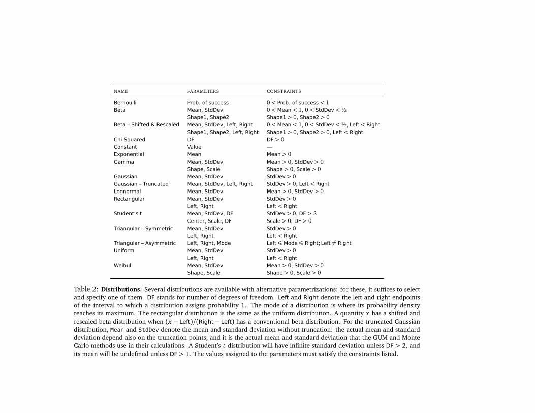
Table 2: Distributions. Several distributions are available with alternative parametrizations: for these, it suffices to selectand specify one of them. DF stands for number of degrees of freedom. Left and Right denote the left and right endpointsof the interval to which a distribution assigns probability 1. The mode of a distribution is where its probability densityreaches its maximum. The rectangular distribution is the same as the uniform distribution. A quantity x has a shifted andrescaled beta distribution when (x − Left)/(Right− Left) has a conventional beta distribution. For the truncated Gaussiandistribution, Mean and StdDev denote the mean and standard deviation without truncation: the actual mean and standarddeviation depend also on the truncation points, and it is the actual mean and standard deviation that the GUM and MonteCarlo methods use in their calculations. A Student’s t distribution will have infinite standard deviation unless DF > 2, andits mean will be undefined unless DF> 1. The values assigned to the parameters must satisfy the constraints listed.
VERSION 1.3.5 NIST UNCERTAINTY MACHINE
of the median. For a sample of large size n drawn from a continuousdistribution with probability density g, this standard deviation is ap-proximately equal to 1/(2g(M)
pn), where M denotes the true value
of the median.
Also listed are coverage intervals with coverage probabilities 99 %, 95 %,90 %, and 68 %. The interval with 68 % coverage probability is oftencalled a “1-sigma interval”, and the interval with 95 % coverage probabil-ity is often called a “2-sigma interval”: however, these designations areappropriate only when the distribution of the output quantity is approx-imately Gaussian. Next to each interval is listed the value of the corre-sponding coverage factor k (cf. GUM 3.3.7, and GUM 6.2). The values ofk are equal to one half the length of the interval divided by the standarduncertainty.
If the box mentioned in (U-9) above is checked prior to starting the com-putations then these intervals will be centered on the mean of the sampleof values of the output quantity. Otherwise their endpoints will be com-puted as explained in (U-9).
The section pertaining to the Monte Carlo method concludes with a tableof analysis of variance (ANOVA) that lists, for each input quantity, theproportion of u2(y) that the source of uncertainty corresponding to theinput quantity is responsible for, computed under the assumption that theoutput quantity is a linear function of the input quantities [Lafarge andPossolo, 2015].
The line labeled “Residual” lists the proportion of u2(y) that is left unac-counted for when that assumption of linearity does not hold. Therefore,it provides a single-number summary of the accuracy of the approxima-tion to u(y) given by Gauss’s formula, which is Equation (13) in the GUM(Page 21).
The ANOVA table has two columns: the column labeled “w/out Residual”lists the proportions recomputed out of a total that excludes the portiondeemed “residual”. These should be numerically close to the entries inthe similar table that appears at the bottom of the section of results fromthe application of the method described in the GUM.
The results obtained according to the GUM are listed under Gauss’s
Formula (GUM’s Linear Approximation). These include an estimateof the true value of the output quantity and an evaluation of the associ-ated standard uncertainty. The former is computed according to Equa-tion (1) in the GUM, and the latter according to Equation (13), where the
LAFARGE & POSSOLO PAGE 15 OF 46
VERSION 1.3.5 NIST UNCERTAINTY MACHINE
values of the partial derivatives are computed using numerical differen-tiation as implemented in R function grad defined in package numDeriv
[Gilbert and Varadhan, 2016].
Finally, a table shows the sensitivity coefficients as defined in the GUM5.1.3: the values of the first-order partial derivatives of the measurementfunction f evaluated at the estimates of the input quantities.
The same table also shows the percentage contributions that the differentinput quantities make to the squared standard uncertainty of the outputquantity. If the input quantities are uncorrelated, then these contributionsadd up to 100 % approximately. If they are correlated, then the contribu-tions may add up to more or less than 100 %, depending on the absolutevalues and signs of the correlations: in this case, the line labeled Corre-
lations will indicate the percentage of u2(y) that is attributable to thosecorrelations (this percentage is positive if u2(y) is larger than it wouldhave been in the absence of correlations).
• The plot included in the output Web page depicts an estimate of the prob-ability density of the output quantity (smooth, continuous version of ahistogram, drawn in a solid blue line) computed as described by Silver-man [1986] and as implemented in R function density. The plot alsoshows (depicted as a red dashed line) the probability density of the Gaus-sian distribution with the same mean and standard deviation as the MonteCarlo sample of values of the output quantity.
• Below this plot there are five clickable lines of green text that, once clicked,download a file to the local machine.
– Download binary R data file with Monte Carlo values
of output quantity: a binary file with suffix Rd is downloadedthat contains (in variable y) the Monte Carlo sample of values drawnfrom the probability distribution of the output quantity — it can beloaded into R using the function load.
NOTE. When the output quantity is a vector with p ¾ 2 compo-nents, as contemplated in (U-8), the NIST Uncertainty Machinewill produce p tabs with output, labeled Output 1, Output 2,. . . , each structured as described above. A download request,initiated by clicking the green text just mentioned on any of theoutput tabs, will download the values sampled for all p outputs.When this file with results is loaded into R, a list named yListis made available, with p elements named y1, y2, . . . .
LAFARGE & POSSOLO PAGE 16 OF 46

VERSION 1.3.5 NIST UNCERTAINTY MACHINE
– Download a text file with Monte Carlo values of output
quantity: a plain text file is downloaded that contains the MonteCarlo sample of values drawn from the probability distribution of theoutput quantity; since preparing this file involves converting the bi-nary file mentioned above into a plain text version, some noticeabletime may elapse before the download actually begins.
NOTE. When the output quantity is a vector with p ¾ 2 compo-nents, as contemplated in (U-8), the NIST Uncertainty Machinewill produce p tabs with output, labeled Output 1, Output 2,. . . , each structured as described above. A download request ini-tiated by clicking the green text just mentioned on any of theoutput tabs will download the values sampled for all p outputs,arranged into a plain text file with as many rows as the samplesize of the Monte Carlo sample, and with p values per line, sep-arated from each other by blank spaces.
– Download text file with numerical results shown on this
page: a plain text file with the same results and layout of the nu-merical results shown on the output Web page.
– Download JPEG file with plot shown on this page: a JPEG filewith the same plot that is displayed on the Web page, showing twoprobability densities.
– Download Configuration File: a plain text file with extension.um that specifies the inputs that were used and that may be reusedas explained in (U-1).
6 Transparency for Validation & Verification
Given a configuration file produced by the NIST Uncertainty Machine, whichhas been saved to the user’s local machine as explained in (U-12) on Page 12,and passing the file name as an argument to FullScriptNUM.R, should producethe same results as when the same configuration file is loaded into the NIST
Uncertainty Machine and run there, provided R has been installed in the localmachine.
Suppose the configuration file is called NUMConfigExample.um. (The defaultextension for configuration files produced by the NIST Uncertainty Machine
is .um, but the file name may be any alphanumeric string that is a legal filename under the applicable operating system — embedded blank spaces arediscouraged — and does not even have to have an extension.
LAFARGE & POSSOLO PAGE 17 OF 46
VERSION 1.3.5 NIST UNCERTAINTY MACHINE
The following command, executed in a terminal window (under Linux or Ma-cOS), or at the Windows command prompt, will replicate the results that thespecified configuration file would produce if loaded into the NIST Uncertainty
Machine and run there. (In Windows other than version 10, click Start, typecmd in the box Search programs and files, and press Enter on the keyboard.In Windows 10 choose Command Prompt from the menu that appears after press-ing WIN+X or right-clicking on the Start button.) Note that $ denotes theterminal prompt, hence is not part of the command:
$ Rscript FullScriptNUM.R NUMConfigExample.um
The script, which is available at https://uncertainty.nist.gov/verification.php, will generate 3 files in the current directory or folder, with the same pre-fix as the configuration file. In the case of the example above, the output fileswould be:
• NUMConfigExample-results.txt: a plain text file with the same resultsand layout of the numerical results shown on the NIST Uncertainty
Machine’s output Web page;
• NUMConfigExample-density.jpg: a JPEG file with the same plot that isdisplayed on the NIST Uncertainty Machine’s output Web page, show-ing the graphs of two probability densities;
• NUMConfigExample-values.Rd: a binary R data file with the replicatesof the input quantities, and with the corresponding values of the outputquantity, corresponding to the Monte Carlo method of the GUM-S1. InR, the command load(“NUMConfigExample-values.Rd”) will create asmany vectors as there are input quantities, with their names as specifiedin the configuration file, and a vector named y with the values of theoutput quantity.
The script will install any necessary R packages that may not have been previ-ously installed in the local version of the R system. The script first writes itsversion number onto the terminal window, which should be matched to theversion of the NIST Uncertainty Machine displayed at the top of the page ofthe web application, for example: NIST Validation & Verification Script
Version 1.3.5
LAFARGE & POSSOLO PAGE 18 OF 46
VERSION 1.3.5 NIST UNCERTAINTY MACHINE
7 Example — Thermal Expansion Coefficient
To measure the coefficient of linear thermal expansion of a cylindrical copperbar, the length L0 = 1.4999m of the bar was measured with the bar at tem-perature T0 = 288.15 K, and then again at temperature T1 = 373.10K, yieldingL1 = 1.5021 m. The measurement model is A= (L1 − L0)/
L0(T1 − T0)
.
For the purpose of this illustration we will assume that the input quantities arelike (scaled and shifted) Student’s t random variables with 3 degrees of free-dom, with means equal to the measured values given, and standard deviationsu(L0) = 0.0001 m, u(L1) = 0.0002m, u(T0) = 0.02 K, and u(T1) = 0.05K.
This modeling assumption is appropriate when the estimates of the input quan-tities are averages of 4 determinations made under conditions of repeatability,which may be regarded as samples from Gaussian distributions, and the associ-ated uncertainties result from Type A evaluations, and are what the GUM calls“experimental standard deviation of the mean”, computed according to Equa-tion (5) in the GUM.
To load the specifications for this example into the NIST Uncertainty Machine,click here. The GUM’s approach yields α = 1.727× 10⁻⁵ K−1 and u(α) =2× 10⁻⁶ K−1, and the Monte Carlo method reproduces these results. Figure 2on Page 20 reflects these facts, and lists the results.
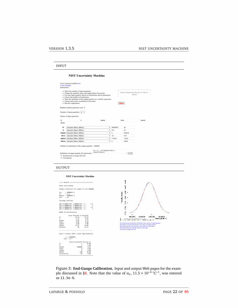
8 Example — End-Gauge Calibration
In Example H.1 of the GUM (which is reconsidered by Guthrie et al. [2009]),the measurement model is l = lS + d − lS[(δα)θ +αS(δθ )], where δα and δθeach denotes a single input quantity, not a product of two input quantities.
The estimates and standard measurement uncertainties of the input quantitiesare listed in Table 3. For the Monte Carlo method, we model the input quantitiesas independent Gaussian random variables with means and standard deviationsequal to these estimates and standard measurement uncertainties. To load thespecifications for this example into the NIST Uncertainty Machine, click here.
The GUM’s approach yields l = 50000 838nm and u(l) = 32 nm, while theMonte Carlo method reproduces the value for l but evaluates u(l) = 34 nm.Refer to Figure 3 on Page22.
The GUM (Page 84) gives (50000 745nm, 50000 931nm) as an approximate99 % coverage interval for l, and the results of the Monte Carlo method confirmthis coverage probability. If the user chooses a coverage interval that is proba-
LAFARGE & POSSOLO PAGE 19 OF 46

VERSION 1.3.5 NIST UNCERTAINTY MACHINE
INPUT
NIST Uncertainty Machine
User's manual available here.
Instructions :
Select the number of input quantities.Change the quantity names and update them if necessary.For each input quantity choose its distribution and its parameters.Choose the number of realizations.Write the definition of the output quantity in a valid R expression.Choose and set the correlations if necessary.Run the computation.
Drop configuration file here or click toupload
Reset
Random number generator seed: 5 Number of input quantities: 4
Names of input quantities:
L0 T0 L1 T1
L0 Student t (Mean, StdDev, No. of degrees of freedom) 1.4999 0.0001 3
T0 Student t (Mean, StdDev, No. of degrees of freedom) 288.15 0.02 3
L1 Student t (Mean, StdDev, No. of degrees of freedom) 1.5021 0.0002 3
T1 Student t (Mean, StdDev, No. of degrees of freedom) 373.10 0.05 3
Number of realizations of the output quantity: 1000000
Definition of output quantity (R expression): (L1-L0) / (L0*(T1-T0))
- + Symmetrical coverage intervals Correlations
Run the computation
Load examples
OUTPUT
===== RESULTS ============================== Monte Carlo Method Summary statistics for sample of size 1000000 ave = 1.727e-05 sd = 1.7e-06 median = 1.727e-05 mad = 1.2e-06 Coverage intervals 99% ( 1.2e-05, 2.3e-05) k = 3.2 95% ( 1.4e-05, 2.05e-05) k = 1.9 90% (1.48e-05, 1.97e-05) k = 1.4 68% ( 1.6e-05, 1.86e-05) k = 0.75 ANOVA (% Contributions) w/out Residual w/ Residual L0 20.48 20.48 T0 0.00 0.00 L1 79.52 79.52 T1 0.00 0.00 Residual NA 0.00 -------------------------------------------- Gauss's Formula (GUM's Linear Approximation) y = 1.727e-05 u(y) = 1.8e-06 SensitivityCoeffs Percent.u2 L0 -7.9e-03 2.0e+01 T0 2.0e-07 5.4e-04 L1 7.8e-03 8.0e+01 T1 -2.0e-07 3.4e-03 Correlations NA 0.0e+00 ============================================
Download binary R data file with Monte Carlo values of output quantity Download a text file with Monte Carlo values of output quantity Download text file with numerical results shown on this page Download JPEG file with plot shown on this page Download configuration file
NIST Uncertainty Machine
Figure 2: Thermal Expansion Coefficient. Input and output Web pages forthe example discussed in §7.
LAFARGE & POSSOLO PAGE 20 OF 46
VERSION 1.3.5 NIST UNCERTAINTY MACHINE
QUANTITY x u(x)
lS 50 000623 nm 25 nmd 215 nm 9.7 nmδα 0 C−1 0.58× 10⁻⁶ C−1
θ −0.1 C 0.41 CαS 11.5× 10⁻⁶ C−1 1.2× 10⁻⁶ C−1
δθ 0 C 0.029 C
Table 3: End-Gauge Calibration. Estimates and standard measurementuncertainties for the input quantities in the measurement model of Exam-ple H.1 in the GUM.
bilistically symmetric (meaning that it leaves 0.5 % of the Monte Carlo sampleuncovered on both sides), then the Monte Carlo method produces (50000 749nm,50 000927 nm) as 99 % coverage interval, which happens not be quite centeredat the estimate of y .
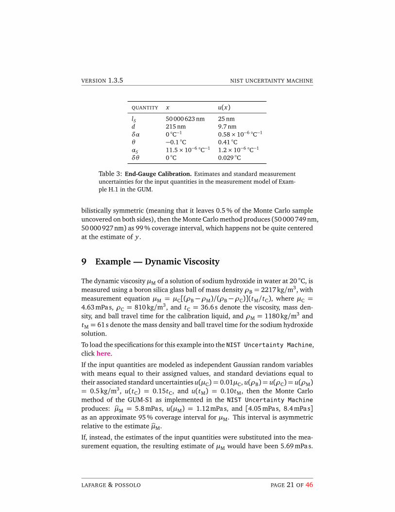
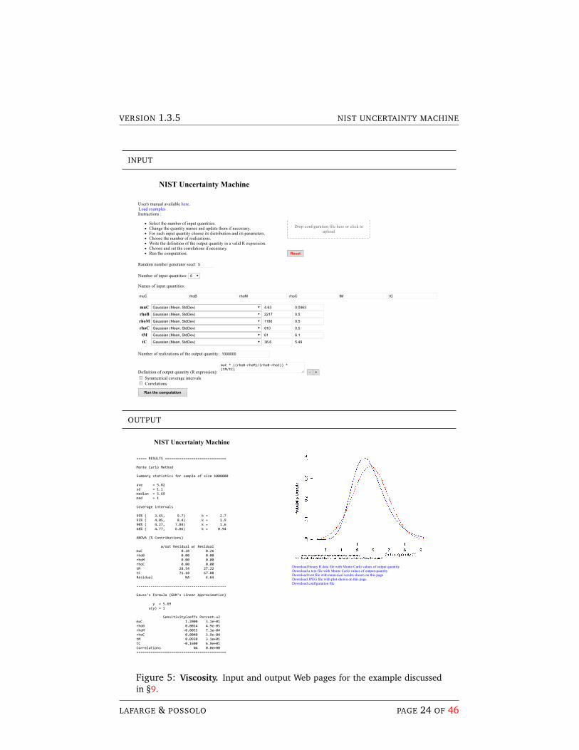
9 Example — Dynamic Viscosity
The dynamic viscosity µM of a solution of sodium hydroxide in water at 20 C, ismeasured using a boron silica glass ball of mass density ρB = 2217 kg/m3, withmeasurement equation µM = µC[(ρB −ρM)/(ρB −ρC)](tM/tC), where µC =4.63 mPas, ρC = 810kg/m3, and tC = 36.6 s denote the viscosity, mass den-sity, and ball travel time for the calibration liquid, and ρM = 1180 kg/m3 andtM = 61s denote the mass density and ball travel time for the sodium hydroxidesolution.
To load the specifications for this example into the NIST Uncertainty Machine,click here.
If the input quantities are modeled as independent Gaussian random variableswith means equal to their assigned values, and standard deviations equal totheir associated standard uncertainties u(µC) = 0.01µC, u(ρB) = u(ρC) = u(ρM)= 0.5 kg/m3, u(tC) = 0.15tC, and u(tM) = 0.10tM, then the Monte Carlomethod of the GUM-S1 as implemented in the NIST Uncertainty Machine
produces: bµM = 5.8 mPas, u(µM) = 1.12mPa s, and [4.05 mPas, 8.4 mPas]as an approximate 95 % coverage interval for µM. This interval is asymmetricrelative to the estimate bµM.
If, instead, the estimates of the input quantities were substituted into the mea-surement equation, the resulting estimate of µM would have been 5.69 mPas.
LAFARGE & POSSOLO PAGE 21 OF 46
VERSION 1.3.5 NIST UNCERTAINTY MACHINE
INPUT
NIST Uncertainty Machine
User's manual available here.
Instructions :
Select the number of input quantities.Change the quantity names and update them if necessary.For each input quantity choose its distribution and its parameters.Choose the number of realizations.Write the definition of the output quantity in a valid R expression.Choose and set the correlations if necessary.Run the computation.
Drop configuration file here or click toupload
Reset
Random number generator seed: 5 Number of input quantities: 6
Names of input quantities:
lS d dalpha theta alphaS
dtheta
lS Gaussian (Mean, StdDev) 50000623 25
d Gaussian (Mean, StdDev) 215 9.7
dalpha Gaussian (Mean, StdDev) 0 0.58e-6
theta Gaussian (Mean, StdDev) -0.1 0.41
alphaS Gaussian (Mean, StdDev) 11.5e-6 1.2e-6
dtheta Gaussian (Mean, StdDev) 0 0.029
Number of realizations of the output quantity: 1000000
Definition of output quantity (R expression): lS + d - lS*(dalpha*theta + alphaS*dtheta)
- + Symmetrical coverage intervals Correlations
Load examples
OUTPUT
===== RESULTS ============================== Monte Carlo Method Summary statistics for sample of size 1000000 ave = 50000837.9 sd = 33.9 median = 50000837.9 mad = 34 Coverage intervals 99% (5.00007e+07, 5.00009e+07) k = 2.6 95% (5.00008e+07, 5.00009e+07) k = 2 90% (5.00008e+07, 5.00009e+07) k = 1.7 68% (5.00008e+07, 5.00009e+07) k = 1 ANOVA (% Contributions) w/out Residual w/ Residual lS 62.36 54.52 d 9.23 8.07 dalpha 0.85 0.75 theta 0.00 0.00 alphaS 0.00 0.00 dtheta 27.55 24.09 Residual NA 12.57 -------------------------------------------- Gauss's Formula (GUM's Linear Approximation) y = 50000838 u(y) = 31.7 SensitivityCoeffs Percent.u2 lS 1 62.00 d 1 9.40 dalpha 5000000 0.84 theta 0 0.00 alphaS 0 0.00 dtheta -580 28.00 Correlations NA 0.00 ============================================
Download binary R data file with Monte Carlo values of output quantity Download a text file with Monte Carlo values of output quantity Download text file with numerical results shown on this page Download JPEG file with plot shown on this page Download configuration file
NIST Uncertainty Machine
Figure 3: End-Gauge Calibration. Input and output Web pages for the exam-ple discussed in §8. Note that the value of αS , 11.5× 10⁻⁶ C−1, was enteredas 11.5e-6.
LAFARGE & POSSOLO PAGE 22 OF 46
VERSION 1.3.5 NIST UNCERTAINTY MACHINE
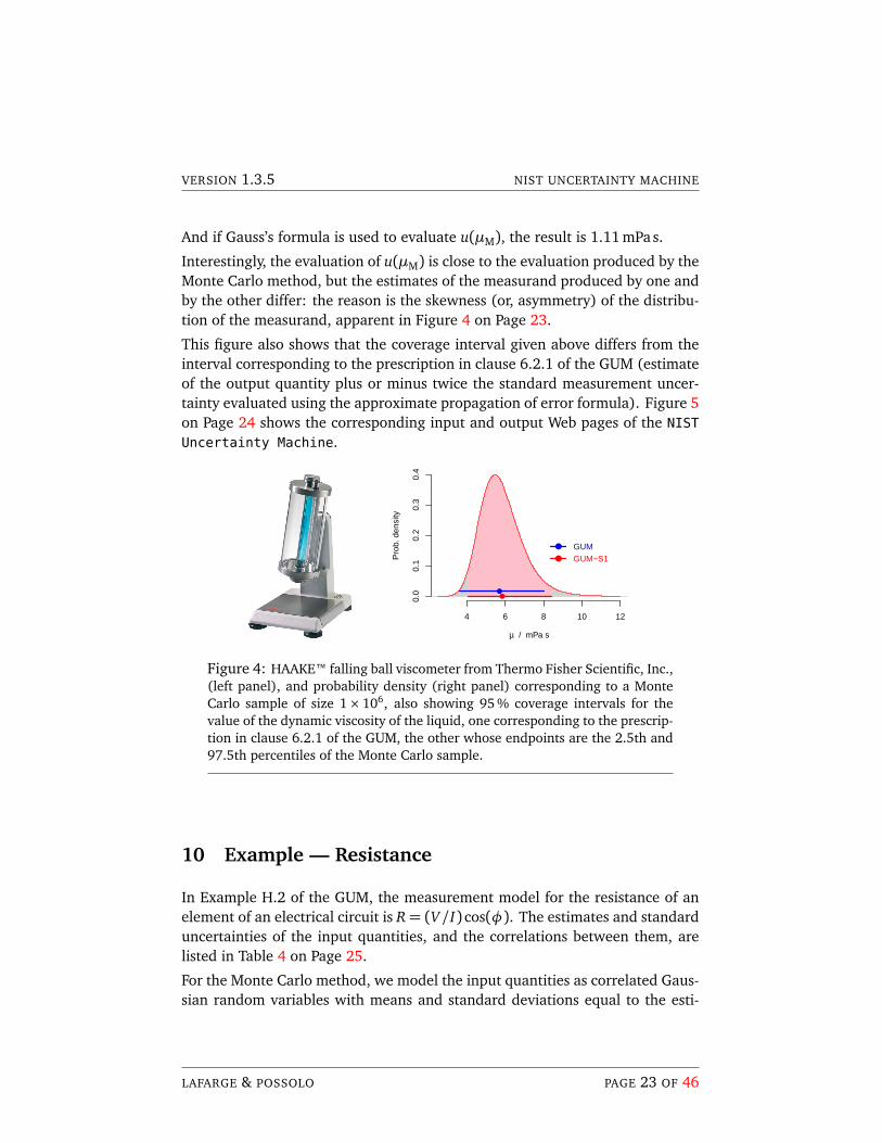
And if Gauss’s formula is used to evaluate u(µM), the result is 1.11 mPas.
Interestingly, the evaluation of u(µM) is close to the evaluation produced by theMonte Carlo method, but the estimates of the measurand produced by one andby the other differ: the reason is the skewness (or, asymmetry) of the distribu-tion of the measurand, apparent in Figure 4 on Page 23.
This figure also shows that the coverage interval given above differs from theinterval corresponding to the prescription in clause 6.2.1 of the GUM (estimateof the output quantity plus or minus twice the standard measurement uncer-tainty evaluated using the approximate propagation of error formula). Figure 5on Page 24 shows the corresponding input and output Web pages of the NIST
Uncertainty Machine.
4 6 8 10 12
0.0
0.1
0.2
0.3
0.4
µ / mPa s
Pro
b. d
ensi
ty
GUMGUM−S1
Figure 4: HAAKE™ falling ball viscometer from Thermo Fisher Scientific, Inc.,(left panel), and probability density (right panel) corresponding to a MonteCarlo sample of size 1× 10⁶, also showing 95 % coverage intervals for thevalue of the dynamic viscosity of the liquid, one corresponding to the prescrip-tion in clause 6.2.1 of the GUM, the other whose endpoints are the 2.5th and97.5th percentiles of the Monte Carlo sample.
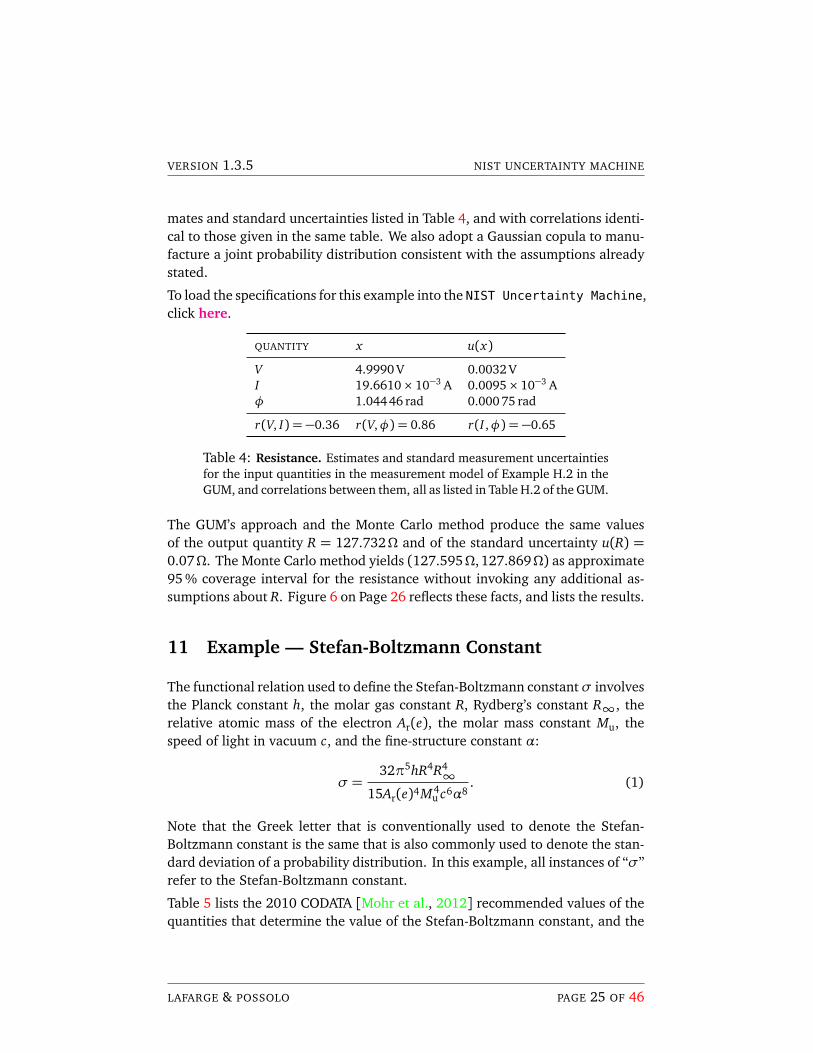
10 Example — Resistance
In Example H.2 of the GUM, the measurement model for the resistance of anelement of an electrical circuit is R= (V/I) cos(φ). The estimates and standarduncertainties of the input quantities, and the correlations between them, arelisted in Table 4 on Page 25.
For the Monte Carlo method, we model the input quantities as correlated Gaus-sian random variables with means and standard deviations equal to the esti-
LAFARGE & POSSOLO PAGE 23 OF 46
VERSION 1.3.5 NIST UNCERTAINTY MACHINE
INPUT
NIST Uncertainty Machine
User's manual available here.
Instructions :
Select the number of input quantities.Change the quantity names and update them if necessary.For each input quantity choose its distribution and its parameters.Choose the number of realizations.Write the definition of the output quantity in a valid R expression.Choose and set the correlations if necessary.Run the computation.
Drop configuration file here or click toupload
Reset
Random number generator seed: 5 Number of input quantities: 6
Names of input quantities:
muC rhoB rhoM rhoC tM tC
muC Gaussian (Mean, StdDev) 4.63 0.0463
rhoB Gaussian (Mean, StdDev) 2217 0.5
rhoM Gaussian (Mean, StdDev) 1180 0.5
rhoC Gaussian (Mean, StdDev) 810 0.5
tM Gaussian (Mean, StdDev) 61 6.1
tC Gaussian (Mean, StdDev) 36.6 5.49
Number of realizations of the output quantity: 1000000
Definition of output quantity (R expression): muC * ((rhoB-rhoM)/(rhoB-rhoC)) * (tM/tC)
- + Symmetrical coverage intervals Correlations
Run the computation
Load examples
OUTPUT
===== RESULTS ============================== Monte Carlo Method Summary statistics for sample of size 1000000 ave = 5.82 sd = 1.1 median = 5.69 mad = 1 Coverage intervals 99% ( 3.65, 9.7) k = 2.7 95% ( 4.05, 8.4) k = 1.9 90% ( 4.27, 7.84) k = 1.6 68% ( 4.77, 6.86) k = 0.94 ANOVA (% Contributions) w/out Residual w/ Residual muC 0.28 0.26 rhoB 0.00 0.00 rhoM 0.00 0.00 rhoC 0.00 0.00 tM 28.54 27.22 tC 71.18 67.88 Residual NA 4.64 -------------------------------------------- Gauss's Formula (GUM's Linear Approximation) y = 5.69 u(y) = 1 SensitivityCoeffs Percent.u2 muC 1.2000 3.1e-01 rhoB 0.0014 4.9e-05 rhoM -0.0055 7.1e-04 rhoC 0.0040 3.9e-04 tM 0.0930 3.1e+01 tC -0.1600 6.9e+01 Correlations NA 0.0e+00 ============================================
Download binary R data file with Monte Carlo values of output quantity Download a text file with Monte Carlo values of output quantity Download text file with numerical results shown on this page Download JPEG file with plot shown on this page Download configuration file
NIST Uncertainty Machine
Figure 5: Viscosity. Input and output Web pages for the example discussedin §9.
LAFARGE & POSSOLO PAGE 24 OF 46
VERSION 1.3.5 NIST UNCERTAINTY MACHINE
mates and standard uncertainties listed in Table 4, and with correlations identi-cal to those given in the same table. We also adopt a Gaussian copula to manu-facture a joint probability distribution consistent with the assumptions alreadystated.
To load the specifications for this example into the NIST Uncertainty Machine,click here.
QUANTITY x u(x)
V 4.9990 V 0.0032 VI 19.6610× 10⁻³ A 0.0095× 10⁻³ Aφ 1.04446 rad 0.00075 rad
r(V, I) = −0.36 r(V,φ) = 0.86 r(I ,φ) = −0.65
Table 4: Resistance. Estimates and standard measurement uncertaintiesfor the input quantities in the measurement model of Example H.2 in theGUM, and correlations between them, all as listed in Table H.2 of the GUM.
The GUM’s approach and the Monte Carlo method produce the same valuesof the output quantity R = 127.732Ω and of the standard uncertainty u(R) =0.07Ω. The Monte Carlo method yields (127.595Ω, 127.869Ω) as approximate95 % coverage interval for the resistance without invoking any additional as-sumptions about R. Figure 6 on Page 26 reflects these facts, and lists the results.
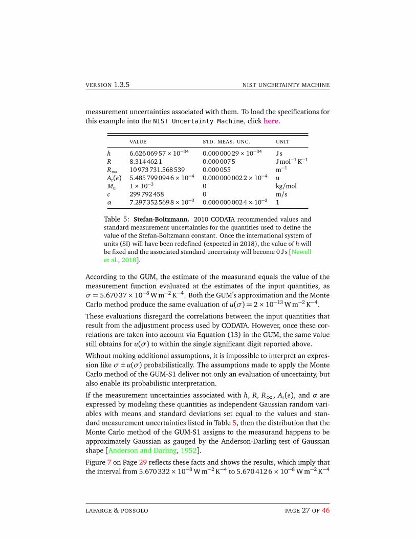
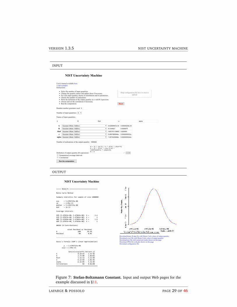
11 Example — Stefan-Boltzmann Constant
The functional relation used to define the Stefan-Boltzmann constantσ involvesthe Planck constant h, the molar gas constant R, Rydberg’s constant R∞, therelative atomic mass of the electron Ar(e), the molar mass constant Mu, thespeed of light in vacuum c, and the fine-structure constant α:
σ =32π5hR4R4
∞
15Ar(e)4M4u c6α8
. (1)
Note that the Greek letter that is conventionally used to denote the Stefan-Boltzmann constant is the same that is also commonly used to denote the stan-dard deviation of a probability distribution. In this example, all instances of “σ”refer to the Stefan-Boltzmann constant.
Table 5 lists the 2010 CODATA [Mohr et al., 2012] recommended values of thequantities that determine the value of the Stefan-Boltzmann constant, and the
LAFARGE & POSSOLO PAGE 25 OF 46
VERSION 1.3.5 NIST UNCERTAINTY MACHINE
INPUT
NIST Uncertainty Machine
User's manual available here.
Instructions :
Select the number of input quantities.Change the quantity names and update them if necessary.For each input quantity choose its distribution and its parameters.Choose the number of realizations.Write the definition of the output quantity in a valid R expression.Choose and set the correlations if necessary.Run the computation.
Drop configuration file here or click toupload
Reset
Random number generator seed: 5 Number of input quantities: 3
Names of input quantities:
V I phi
V Gaussian (Mean, StdDev) 4.9990 0.0032
I Gaussian (Mean, StdDev) 19.6610e-3 0.0095e-3
phi Gaussian (Mean, StdDev) 1.04446 0.00075
Number of realizations of the output quantity: 1000000
Definition of output quantity (R expression): (V/I)*cos(phi)
- + Symmetrical coverage intervals Correlations
V I phiV 1 -0.36 0.86
I 1 -0.65
phi 1
Gaussian Copula
Run the computation
Load examples
OUTPUT
===== RESULTS ============================== Monte Carlo Method Summary statistics for sample of size 1000000 ave = 127.732 sd = 0.0699 median = 127.732 mad = 0.07 Coverage intervals 99% ( 127.55, 127.91) k = 2.6 95% ( 127.59, 127.87) k = 2 90% ( 127.62, 127.85) k = 1.6 68% ( 127.662, 127.802) k = 1 ANOVA (% Contributions) w/out Residual w/ Residual V 29.31 29.31 I 0.13 0.13 phi 70.56 70.56 Residual NA 0.00 -------------------------------------------- Gauss's Formula (GUM's Linear Approximation) y = 127.732 u(y) = 0.07 SensitivityCoeffs Percent.u2 V 26 140 I -6500 78 phi -220 560 Correlations NA -670 ============================================
Download binary R data file with Monte Carlo values of output quantity Download a text file with Monte Carlo values of output quantity Download text file with numerical results shown on this page Download JPEG file with plot shown on this page Download configuration file
NIST Uncertainty Machine
Figure 6: Resistance. Input and output Web pages for the example discussed in §10.Note that, in this case, the NIST Uncertainty Machine reconfigured its graphical userinterface automatically to accommodate the correlations that had to be specified.
LAFARGE & POSSOLO PAGE 26 OF 46
VERSION 1.3.5 NIST UNCERTAINTY MACHINE
measurement uncertainties associated with them. To load the specifications forthis example into the NIST Uncertainty Machine, click here.
VALUE STD. MEAS. UNC. UNIT
h 6.626069 57× 10−34 0.000 00029× 10−34 J sR 8.314462 1 0.000 0075 J mol−1 K−1
R∞ 10973 731.568539 0.000 055 m−1
Ar(e) 5.485799 0946× 10−4 0.000 000002 2× 10⁻⁴ uMu 1× 10⁻³ 0 kg/molc 299792 458 0 m/sα 7.297352 5698× 10−3 0.000 000002 4× 10⁻³ 1
Table 5: Stefan-Boltzmann. 2010 CODATA recommended values andstandard measurement uncertainties for the quantities used to define thevalue of the Stefan-Boltzmann constant. Once the international system ofunits (SI) will have been redefined (expected in 2018), the value of h willbe fixed and the associated standard uncertainty will become 0 J s [Newellet al., 2018].
According to the GUM, the estimate of the measurand equals the value of themeasurement function evaluated at the estimates of the input quantities, asσ = 5.670 37× 10−8 W m−2 K−4. Both the GUM’s approximation and the MonteCarlo method produce the same evaluation of u(σ) = 2× 10⁻¹³ W m−2 K−4.
These evaluations disregard the correlations between the input quantities thatresult from the adjustment process used by CODATA. However, once these cor-relations are taken into account via Equation (13) in the GUM, the same valuestill obtains for u(σ) to within the single significant digit reported above.
Without making additional assumptions, it is impossible to interpret an expres-sion like σ± u(σ) probabilistically. The assumptions made to apply the MonteCarlo method of the GUM-S1 deliver not only an evaluation of uncertainty, butalso enable its probabilistic interpretation.
If the measurement uncertainties associated with h, R, R∞, Ar(e), and α areexpressed by modeling these quantities as independent Gaussian random vari-ables with means and standard deviations set equal to the values and stan-dard measurement uncertainties listed in Table 5, then the distribution that theMonte Carlo method of the GUM-S1 assigns to the measurand happens to beapproximately Gaussian as gauged by the Anderson-Darling test of Gaussianshape [Anderson and Darling, 1952].
Figure 7 on Page 29 reflects these facts and shows the results, which imply thatthe interval from 5.670332× 10⁻⁸ W m−2 K−4 to 5.670412 6× 10⁻⁸ W m−2 K−4
LAFARGE & POSSOLO PAGE 27 OF 46
VERSION 1.3.5 NIST UNCERTAINTY MACHINE
is a coverage interval for σ with approximate 95 % coverage probability.
Two of the inputs, Mu and c, have zero standard uncertainty. Since the NIST
Uncertainty Machine requires standard deviations to be strictly positive, theuser may either assign very small values to them, or they may be removed fromthe list of input quantities and their values entered as constants in the expressionthat defines the output quantity, as shown in the upper panel of Figure 7 onPage 29.
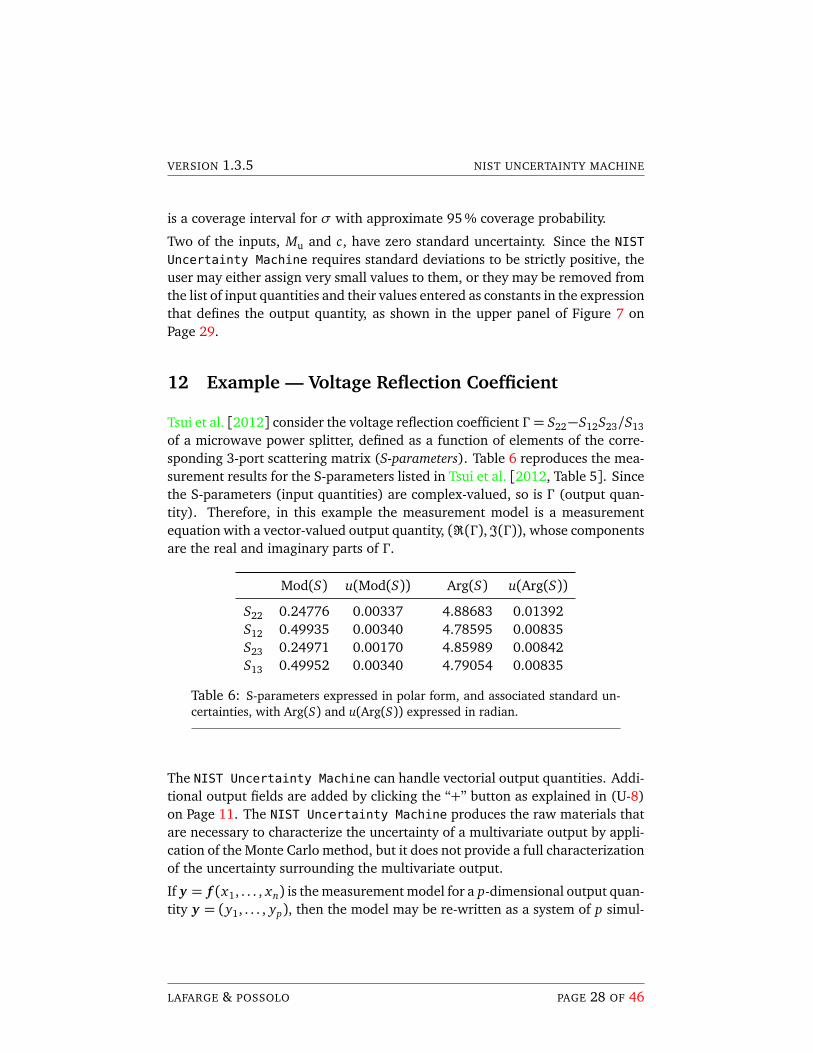
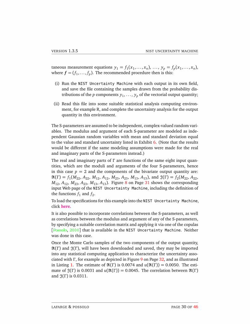
12 Example — Voltage Reflection Coefficient
Tsui et al. [2012] consider the voltage reflection coefficient Γ = S22−S12S23/S13of a microwave power splitter, defined as a function of elements of the corre-sponding 3-port scattering matrix (S-parameters). Table 6 reproduces the mea-surement results for the S-parameters listed in Tsui et al. [2012, Table 5]. Sincethe S-parameters (input quantities) are complex-valued, so is Γ (output quan-tity). Therefore, in this example the measurement model is a measurementequation with a vector-valued output quantity, (ℜ(Γ ),ℑ(Γ )), whose componentsare the real and imaginary parts of Γ .
Mod(S) u(Mod(S)) Arg(S) u(Arg(S))
S22 0.24776 0.00337 4.88683 0.01392S12 0.49935 0.00340 4.78595 0.00835S23 0.24971 0.00170 4.85989 0.00842S13 0.49952 0.00340 4.79054 0.00835
Table 6: S-parameters expressed in polar form, and associated standard un-certainties, with Arg(S) and u(Arg(S)) expressed in radian.
The NIST Uncertainty Machine can handle vectorial output quantities. Addi-tional output fields are added by clicking the “+” button as explained in (U-8)on Page 11. The NIST Uncertainty Machine produces the raw materials thatare necessary to characterize the uncertainty of a multivariate output by appli-cation of the Monte Carlo method, but it does not provide a full characterizationof the uncertainty surrounding the multivariate output.
If y = f (x1, . . . , xn) is the measurement model for a p-dimensional output quan-tity y = (y1, . . . , yp), then the model may be re-written as a system of p simul-
LAFARGE & POSSOLO PAGE 28 OF 46
VERSION 1.3.5 NIST UNCERTAINTY MACHINE
INPUT
NIST Uncertainty Machine
User's manual available here.
Instructions :
Select the number of input quantities.Change the quantity names and update them if necessary.For each input quantity choose its distribution and its parameters.Choose the number of realizations.Write the definition of the output quantity in a valid R expression.Choose and set the correlations if necessary.Run the computation.
Drop configuration file here or click toupload
Reset
Random number generator seed: 5 Number of input quantities: 5
Names of input quantities:
h R Rinf e alpha
h Gaussian (Mean, StdDev) 6.62606957e-34 0.00000029e-34
R Gaussian (Mean, StdDev) 8.3144621 0.0000075
Rinf Gaussian (Mean, StdDev) 0.000055
e Gaussian (Mean, StdDev)
alpha Gaussian (Mean, StdDev)
Number of realizations of the output quantity: 1000000
Definition of output quantity (R expression):
N = 32 * (pi^5) * h * (R^4) * (Rinf^4) D = 15 * (e^4) * ((1e-3)^4) * (299792458^6) * (alpha^8) N / D
- + Symmetrical coverage intervals Correlations
Run the computation
10973731.56853
5.4857990946e-4 0.0000000022e-4
7.2973525698e-3 0.0000000024e-3
Load examples
OUTPUT
===== RESULTS ============================== Monte Carlo Method Summary statistics for sample of size 1000000 ave = 5.6703725e-08 sd = 2.05e-13 median = 5.6703725e-08 mad = 2e-13 Coverage intervals 99% (5.67032e-08, 5.67043e-08) k = 2.6 95% (5.67033e-08, 5.67041e-08) k = 2 90% (5.67034e-08, 5.67041e-08) k = 1.6 68% (5.67035e-08, 5.67039e-08) k = 1 ANOVA (% Contributions) w/out Residual w/ Residual R 100 99.99 Residual NA 0.01 -------------------------------------------- Gauss's Formula (GUM's Linear Approximation) y = 5.6703725e-08 u(y) = 2.05e-13 SensitivityCoeffs Percent.u2 h 8.6e+25 1.5e-02 R 2.7e-08 1.0e+02 Rinf 2.1e-14 3.1e-09 e -4.1e-04 2.0e-05 alpha -6.2e-05 5.3e-05 Correlations NA 0.0e+00 ============================================
Download binary R data file with Monte Carlo values of output quantity Download a text file with Monte Carlo values of output quantity Download text file with numerical results shown on this page Download JPEG file with plot shown on this page Download configuration file
NIST Uncertainty Machine
Figure 7: Stefan-Boltzmann Constant. Input and output Web pages for theexample discussed in §11.
LAFARGE & POSSOLO PAGE 29 OF 46
VERSION 1.3.5 NIST UNCERTAINTY MACHINE
taneous measurement equations y1 = f1(x1, . . . , xn), . . . , yp = fp(x1, . . . , xn),where f = ( f1, . . . , fp). The recommended procedure then is this:
(i) Run the NIST Uncertainty Machine with each output in its own field,and save the file containing the samples drawn from the probability dis-tributions of the p components y1, . . . , yp of the vectorial output quantity;
(ii) Read this file into some suitable statistical analysis computing environ-ment, for example R, and complete the uncertainty analysis for the outputquantity in this environment.
The S-parameters are assumed to be independent, complex-valued random vari-ables. The modulus and argument of each S-parameter are modeled as inde-pendent Gaussian random variables with mean and standard deviation equalto the value and standard uncertainty listed in Exhibit 6. (Note that the resultswould be different if the same modeling assumptions were made for the realand imaginary parts of the S-parameters instead.)
The real and imaginary parts of Γ are functions of the same eight input quan-tities, which are the moduli and arguments of the four S-parameters, hencein this case p = 2 and the components of the bivariate output quantity are:ℜ(Γ ) = f1(M22, A22, M12, A12, M23, A23, M13, A13), and ℑ(Γ ) = f2(M22, A22,M12, A12, M23, A23, M13, A13). Figure 8 on Page 31 shows the correspondinginput Web page of the NIST Uncertainty Machine, including the definition ofthe functions f1 and f2.
To load the specifications for this example into the NIST Uncertainty Machine,click here.
It is also possible to incorporate correlations between the S-parameters, as wellas correlations between the modulus and argument of any of the S-parameters,by specifying a suitable correlation matrix and applying it via one of the copulas[Possolo, 2010] that is available in the NIST Uncertainty Machine. Neitherwas done in this case.
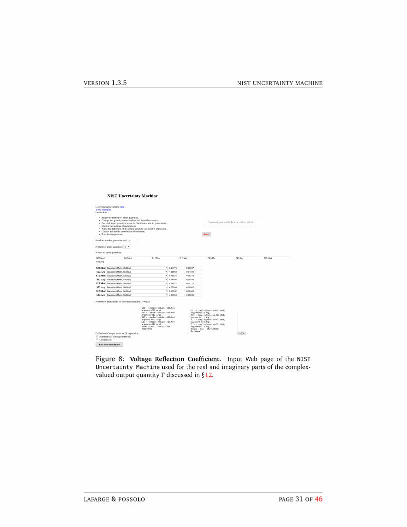
Once the Monte Carlo samples of the two components of the output quantity,ℜ(Γ ) and ℑ(Γ ), will have been downloaded and saved, they may be importedinto any statistical computing application to characterize the uncertainty asso-ciated with Γ , for example as depicted in Figure 9 on Page 32, and as illustratedin Listing 1. The estimate of ℜ(Γ ) is 0.0074 and u(ℜ(Γ )) = 0.0050. The esti-mate of ℑ(Γ ) is 0.0031 and u(ℜ(Γ )) = 0.0045. The correlation between ℜ(Γ )and ℑ(Γ ) is 0.0311.
LAFARGE & POSSOLO PAGE 30 OF 46
VERSION 1.3.5 NIST UNCERTAINTY MACHINE
NIST Uncertainty Machine
User's manual available here.
Instructions :
Select the number of input quantities.Change the quantity names and update them if necessary.For each input quantity choose its distribution and its parameters.Choose the number of realizations.Write the definition of the output quantity in a valid R expression.Choose and set the correlations if necessary.Run the computation.
Drop configuration file here or click to upload
Reset
Random number generator seed: 37 Number of input quantities: 8
Names of input quantities:
S22.Mod S22.Arg S12.Mod S12.Arg S23.Mod S23.Arg S13.Mod
S13.Arg
S22.Mod Gaussian (Mean, StdDev) 0.24776 0.00337
S22.Arg Gaussian (Mean, StdDev) 4.88683 0.01392
S12.Mod Gaussian (Mean, StdDev) 0.49935 0.00340
S12.Arg Gaussian (Mean, StdDev) 4.78595 0.00835
S23.Mod Gaussian (Mean, StdDev) 0.24971 0.00170
S23.Arg Gaussian (Mean, StdDev) 4.85989 0.00842
S13.Mod Gaussian (Mean, StdDev) 0.49952 0.00340
S13.Arg Gaussian (Mean, StdDev) 4.79054 0.00835
Number of realizations of the output quantity: 1000000
Definition of output quantity (R expression):
S22 = complex(modulus=S22.Mod, argument=S22.Arg) S12 = complex(modulus=S12.Mod, argument=S12.Arg) S23 = complex(modulus=S23.Mod, argument=S23.Arg) S13 = complex(modulus=S13.Mod, argument=S13.Arg) Gamma = S22 - S12*S23/S13 Re(Gamma)
S22 = complex(modulus=S22.Mod, argument=S22.Arg) S12 = complex(modulus=S12.Mod, argument=S12.Arg) S23 = complex(modulus=S23.Mod, argument=S23.Arg) S13 = complex(modulus=S13.Mod, argument=S13.Arg) Gamma = S22 - S12*S23/S13 Im(Gamma)
- + Symmetrical coverage intervals Correlations
Run the computation
Load examples
Figure 8: Voltage Reflection Coefficient. Input Web page of the NISTUncertainty Machine used for the real and imaginary parts of the complex-valued output quantity Γ discussed in §12.
LAFARGE & POSSOLO PAGE 31 OF 46
VERSION 1.3.5 NIST UNCERTAINTY MACHINE
Re(Γ)
Im(Γ
)
−0.005 0.000 0.005 0.010 0.015 0.020
−0.
010
−0.
005
0.00
00.
005
0.01
00.
015
Mod(Γ)A
rg(Γ
)
0.000 0.005 0.010 0.015 0.020 0.025
−3
−2
−1
01
23
Figure 9: The left panel shows an estimate of the probability density of the jointdistribution of the real and imaginary parts of Γ , and the right panel shows itscounterpart for the modulus and argument of Γ . The solid (red) curves out-line 95 % coverage regions, and the dashed (red) curves outline 68 % cover-age regions. Their (blue) counterparts, dotted and dash-dotted, are based onthe (obviously erroneous) assumption that the joint bivariate distributions areGaussian.
Listing 1: R code used to characterize the uncertainty associated with Γ
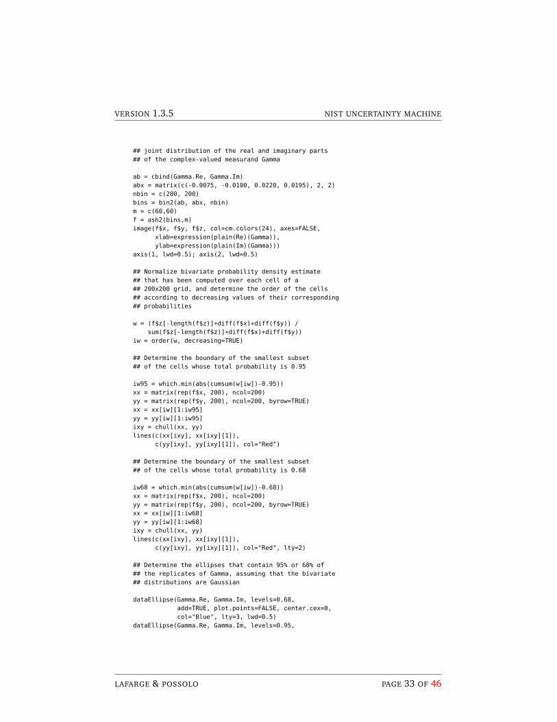
## Read values of output quantities produced in the two runs## of the NIST Uncertainty Machine, assuming that R’s## current working directory is the same that contains## the files with the values of the output quantities
Gamma.Re = scan("NUM-Gamma-Real-Results-Values.txt")Gamma.Im = scan("NUM-Gamma-Imaginary-Results-Values.txt")
Gamma.Mod = Mod(complex(real=Gamma.Re, imaginary=Gamma.Im))Gamma.Arg = Arg(complex(real=Gamma.Re, imaginary=Gamma.Im))
c(mean(Gamma.Re), sd(Gamma.Re))c(mean(Gamma.Im), sd(Gamma.Im))cor(Gamma.Re, Gamma.Im)
require(ash)require(car)
par(mfrow=c(1,2), mar=c(4.5, 4.5, 1.5, 1.5))
## Estimate the probability density of the bivariate
LAFARGE & POSSOLO PAGE 32 OF 46
VERSION 1.3.5 NIST UNCERTAINTY MACHINE
## joint distribution of the real and imaginary parts## of the complex-valued measurand Gamma
ab = cbind(Gamma.Re, Gamma.Im)abx = matrix(c(-0.0075, -0.0100, 0.0220, 0.0195), 2, 2)nbin = c(200, 200)bins = bin2(ab, abx, nbin)m = c(60,60)f = ash2(bins,m)image(f$x, f$y, f$z, col=cm.colors(24), axes=FALSE,
xlab=expression(plain(Re)(Gamma)),ylab=expression(plain(Im)(Gamma)))
axis(1, lwd=0.5); axis(2, lwd=0.5)
## Normalize bivariate probability density estimate## that has been computed over each cell of a## 200x200 grid, and determine the order of the cells## according to decreasing values of their corresponding## probabilities
w = (f$z[-length(f$z)]*diff(f$x)*diff(f$y)) /sum(f$z[-length(f$z)]*diff(f$x)*diff(f$y))
iw = order(w, decreasing=TRUE)
## Determine the boundary of the smallest subset## of the cells whose total probability is 0.95
iw95 = which.min(abs(cumsum(w[iw])-0.95))xx = matrix(rep(f$x, 200), ncol=200)yy = matrix(rep(f$y, 200), ncol=200, byrow=TRUE)xx = xx[iw][1:iw95]yy = yy[iw][1:iw95]ixy = chull(xx, yy)lines(c(xx[ixy], xx[ixy][1]),
c(yy[ixy], yy[ixy][1]), col="Red")
## Determine the boundary of the smallest subset## of the cells whose total probability is 0.68
iw68 = which.min(abs(cumsum(w[iw])-0.68))xx = matrix(rep(f$x, 200), ncol=200)yy = matrix(rep(f$y, 200), ncol=200, byrow=TRUE)xx = xx[iw][1:iw68]yy = yy[iw][1:iw68]ixy = chull(xx, yy)lines(c(xx[ixy], xx[ixy][1]),
c(yy[ixy], yy[ixy][1]), col="Red", lty=2)
## Determine the ellipses that contain 95% or 68% of## the replicates of Gamma, assuming that the bivariate## distributions are Gaussian
dataEllipse(Gamma.Re, Gamma.Im, levels=0.68,add=TRUE, plot.points=FALSE, center.cex=0,col="Blue", lty=3, lwd=0.5)
dataEllipse(Gamma.Re, Gamma.Im, levels=0.95,
LAFARGE & POSSOLO PAGE 33 OF 46
VERSION 1.3.5 NIST UNCERTAINTY MACHINE
add=TRUE, plot.points=FALSE, center.cex=0,col="Blue", lty=4, lwd=0.5)
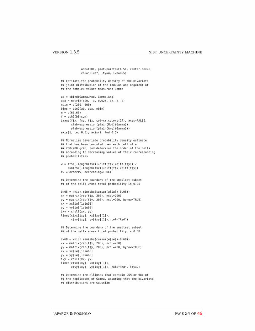
## Estimate the probability density of the bivariate## joint distribution of the modulus and argument of## the complex-valued measurand Gamma
ab = cbind(Gamma.Mod, Gamma.Arg)abx = matrix(c(0, -3, 0.025, 3), 2, 2)nbin = c(200, 200)bins = bin2(ab, abx, nbin)m = c(60,60)f = ash2(bins,m)image(f$x, f$y, f$z, col=cm.colors(24), axes=FALSE,
xlab=expression(plain(Mod)(Gamma)),ylab=expression(plain(Arg)(Gamma)))
axis(1, lwd=0.5); axis(2, lwd=0.5)
## Normalize bivariate probability density estimate## that has been computed over each cell of a## 200x200 grid, and determine the order of the cells## according to decreasing values of their corresponding## probabilities
w = (f$z[-length(f$z)]*diff(f$x)*diff(f$y)) /sum(f$z[-length(f$z)]*diff(f$x)*diff(f$y))
iw = order(w, decreasing=TRUE)
## Determine the boundary of the smallest subset## of the cells whose total probability is 0.95
iw95 = which.min(abs(cumsum(w[iw])-0.95))xx = matrix(rep(f$x, 200), ncol=200)yy = matrix(rep(f$y, 200), ncol=200, byrow=TRUE)xx = xx[iw][1:iw95]yy = yy[iw][1:iw95]ixy = chull(xx, yy)lines(c(xx[ixy], xx[ixy][1]),
c(yy[ixy], yy[ixy][1]), col="Red")
## Determine the boundary of the smallest subset## of the cells whose total probability is 0.68
iw68 = which.min(abs(cumsum(w[iw])-0.68))xx = matrix(rep(f$x, 200), ncol=200)yy = matrix(rep(f$y, 200), ncol=200, byrow=TRUE)xx = xx[iw][1:iw68]yy = yy[iw][1:iw68]ixy = chull(xx, yy)lines(c(xx[ixy], xx[ixy][1]),
c(yy[ixy], yy[ixy][1]), col="Red", lty=2)
## Determine the ellipses that contain 95% or 68% of## the replicates of Gamma, assuming that the bivariate## distributions are Gaussian
LAFARGE & POSSOLO PAGE 34 OF 46
VERSION 1.3.5 NIST UNCERTAINTY MACHINE
dataEllipse(Gamma.Mod, Gamma.Arg, levels=0.68,add=TRUE, plot.points=FALSE, center.cex=0,col="Blue", lty=3, lwd=0.5)
dataEllipse(Gamma.Mod, Gamma.Arg, levels=0.95,add=TRUE, plot.points=FALSE, center.cex=0,col="Blue", lty=4, lwd=0.5)
13 Example — Age of Allende Meteorite
A blinding blue-white fireball, possibly a meteor, turned night into dayacross Mexico and the southwestern United States early today, thenapparently dropped to earth — Washington Post, February 9, 1969.
Table 7 lists isotopic ratios and associated uncertainties for several samplesdrawn from two chondrules of the Allende meteorite [Clarke et al., 1971], tomeasure their absolute age using a geochronometer based on isotopic ratios ofradiogenic lead.
The original data, from Table S4 of Connelly et al. [2012], comprise valuesof R(204Pb/206Pb), R(207Pb/206Pb), and relative expanded uncertainties (withcoverage factor k = 2) expressed as percentages. The isotopic ratios listed inTable 7 were derived from these as R(206Pb/204Pb) = 1/R(204Pb/206Pb) andR(207Pb/204Pb) = R(207Pb/206Pb)R(206Pb/204Pb).
The standard uncertainties listed in Table 7 were derived from the expandeduncertainties in [Connelly et al., 2012, Table S4], by application of the MonteCarlo method, modeling the isotopic ratios as Gaussian random variables, andtaking into account the correlation between R(204Pb/206Pb) and R(207Pb/206Pb)also listed in the aforementioned Table S4. The standard uncertainties listed arethe median absolute deviations from the median, rescaled as per the defaultdefinition of R function mad.
Since 206Pb and 207Pb both are radiogenic, being the end-products of the decayof 235U and 238U, respectively, and 204Pb is primordial, the isotopic ratios inTable 7 may be used as a geochronometer [White, 2015], under the followingassumptions:
(a) The isotopic ratio R(238U/235U) of the parent material is known;
(b) All atoms of 206Pb and 207Pb derive entirely from uranium originally in theparent material, and none have been lost;
LAFARGE & POSSOLO PAGE 35 OF 46
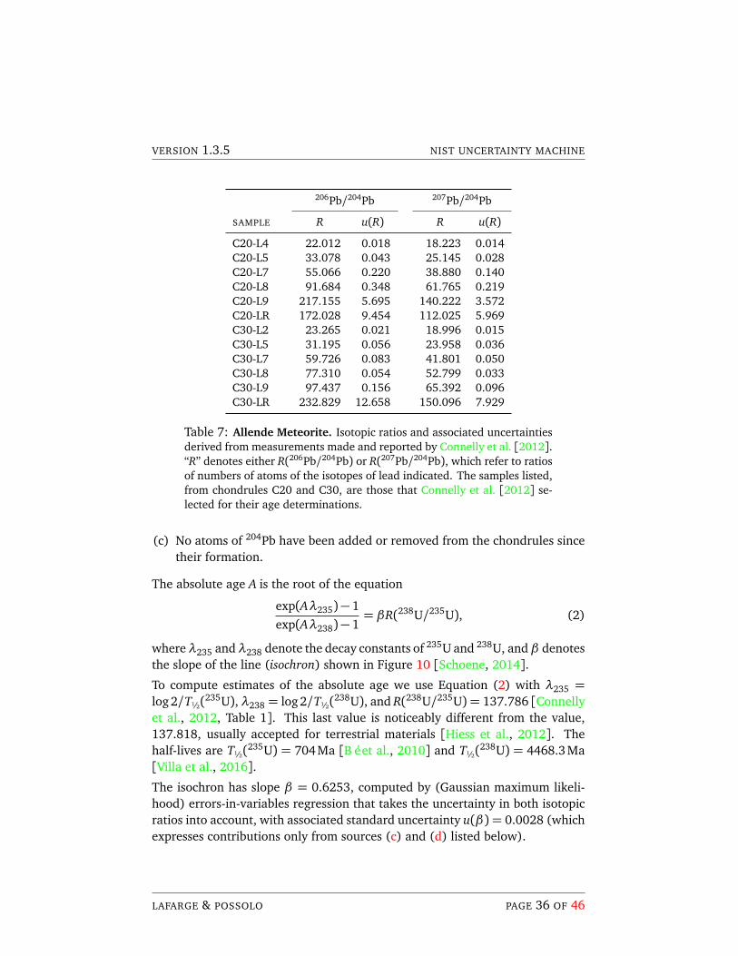
VERSION 1.3.5 NIST UNCERTAINTY MACHINE
206Pb/204Pb 207Pb/204Pb
SAMPLE R u(R) R u(R)
C20-L4 22.012 0.018 18.223 0.014C20-L5 33.078 0.043 25.145 0.028C20-L7 55.066 0.220 38.880 0.140C20-L8 91.684 0.348 61.765 0.219C20-L9 217.155 5.695 140.222 3.572C20-LR 172.028 9.454 112.025 5.969C30-L2 23.265 0.021 18.996 0.015C30-L5 31.195 0.056 23.958 0.036C30-L7 59.726 0.083 41.801 0.050C30-L8 77.310 0.054 52.799 0.033C30-L9 97.437 0.156 65.392 0.096C30-LR 232.829 12.658 150.096 7.929
Table 7: Allende Meteorite. Isotopic ratios and associated uncertaintiesderived from measurements made and reported by Connelly et al. [2012].“R” denotes either R(206Pb/204Pb) or R(207Pb/204Pb), which refer to ratiosof numbers of atoms of the isotopes of lead indicated. The samples listed,from chondrules C20 and C30, are those that Connelly et al. [2012] se-lected for their age determinations.
(c) No atoms of 204Pb have been added or removed from the chondrules sincetheir formation.
The absolute age A is the root of the equation
exp(Aλ235)− 1exp(Aλ238)− 1
= βR(238U/235U), (2)
whereλ235 andλ238 denote the decay constants of 235U and 238U, and β denotesthe slope of the line (isochron) shown in Figure 10 [Schoene, 2014].
To compute estimates of the absolute age we use Equation (2) with λ235 =log 2/T½(235U), λ238 = log2/T½(238U), and R(238U/235U) = 137.786 [Connellyet al., 2012, Table 1]. This last value is noticeably different from the value,137.818, usually accepted for terrestrial materials [Hiess et al., 2012]. Thehalf-lives are T½(235U) = 704Ma [Bé et al., 2010] and T½(238U) = 4468.3Ma[Villa et al., 2016].
The isochron has slope β = 0.6253, computed by (Gaussian maximum likeli-hood) errors-in-variables regression that takes the uncertainty in both isotopicratios into account, with associated standard uncertainty u(β) = 0.0028 (whichexpresses contributions only from sources (c) and (d) listed below).
LAFARGE & POSSOLO PAGE 36 OF 46
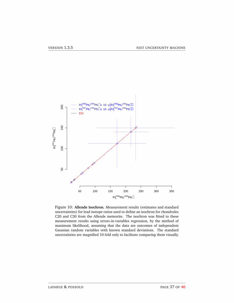
VERSION 1.3.5 NIST UNCERTAINTY MACHINE
50 100 150 200 250 300 350
5010
015
020
0
R(206Pb 204Pb)
R(20
7 Pb
204 P
b)
R(206Pb 204Pb) ± 10 u(R(206Pb 204Pb))R(207Pb 204Pb) ± 10 u(R(207Pb 204Pb))EIV
Figure 10: Allende Isochron. Measurement results (estimates and standarduncertainties) for lead isotope ratios used to define an isochron for chondrulesC20 and C30 from the Allende meteorite. The isochron was fitted to thesemeasurement results using errors-in-variables regression, by the method ofmaximum likelihood, assuming that the data are outcomes of independentGaussian random variables with known standard deviations. The standarduncertainties are magnified 10-fold only to facilitate comparing them visually.
LAFARGE & POSSOLO PAGE 37 OF 46
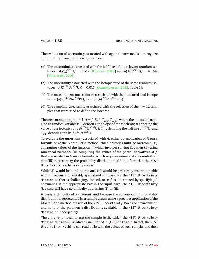
VERSION 1.3.5 NIST UNCERTAINTY MACHINE
The evaluation of uncertainty associated with age estimates needs to recognizecontributions from the following sources:
(a) The uncertainties associated with the half-lives of the relevant uranium iso-topes: u(T½(235U)) = 1 Ma [Bé et al., 2010] and u(T½(238U)) = 4.8 Ma[Villa et al., 2016];
(b) The uncertainty associated with the isotopic ratio of the same uranium iso-topes: u(R(238U/235U)) = 0.013 [Connelly et al., 2012, Table 1];
(c) The measurement uncertainties associated with the measured lead isotoperatios u(R(206Pb/204Pb)) and u(R(207Pb/204Pb));
(d) The sampling uncertainty associated with the selection of the n = 12 sam-ples that were used to define the isochron.
The measurement equation is A= f (B, R, T235, T238), where the inputs are mod-eled as random variables: B denoting the slope of the isochron; R denoting thevalue of the isotopic ratio R(238U/235U); T235 denoting the half-life of 235U; andT238 denoting the half-life of 238U.
To evaluate the uncertainty associated with A, either by application of Gauss’sformula or of the Monte Carlo method, three obstacles must be overcome: (i)computing values of the function f , which involves solving Equation (2) usingnumerical methods; (ii) computing the values of the partial derivatives of fthat are needed in Gauss’s formula, which requires numerical differentiation;and (iii) representing the probability distribution of B in a form that the NIST
Uncertainty Machine can process.
While (i) would be burdensome and (ii) would be practically insurmountablewithout recourse to suitably specialized software, for the NIST Uncertainty
Machine neither is challenging. Indeed, once f is determined by specifying Rcommands in the appropriate box in the input page, the NIST Uncertainty
Machine will have no difficulty addressing (i) or (ii).
B poses a difficulty of a different kind because the corresponding probabilitydistribution is represented by a sample drawn using a previous application of theMonte Carlo method outside of the NIST Uncertainty Machine environment,and none of the parametric distributions available in the NIST Uncertainty
Machine fit it adequately.
Therefore, one needs to use the sample itself, which the NIST Uncertainty
Machine also allows, as already mentioned in (U-5) on Page 9. In fact, the NISTUncertainty Machine can read a file with the values of such sample, and then
LAFARGE & POSSOLO PAGE 38 OF 46
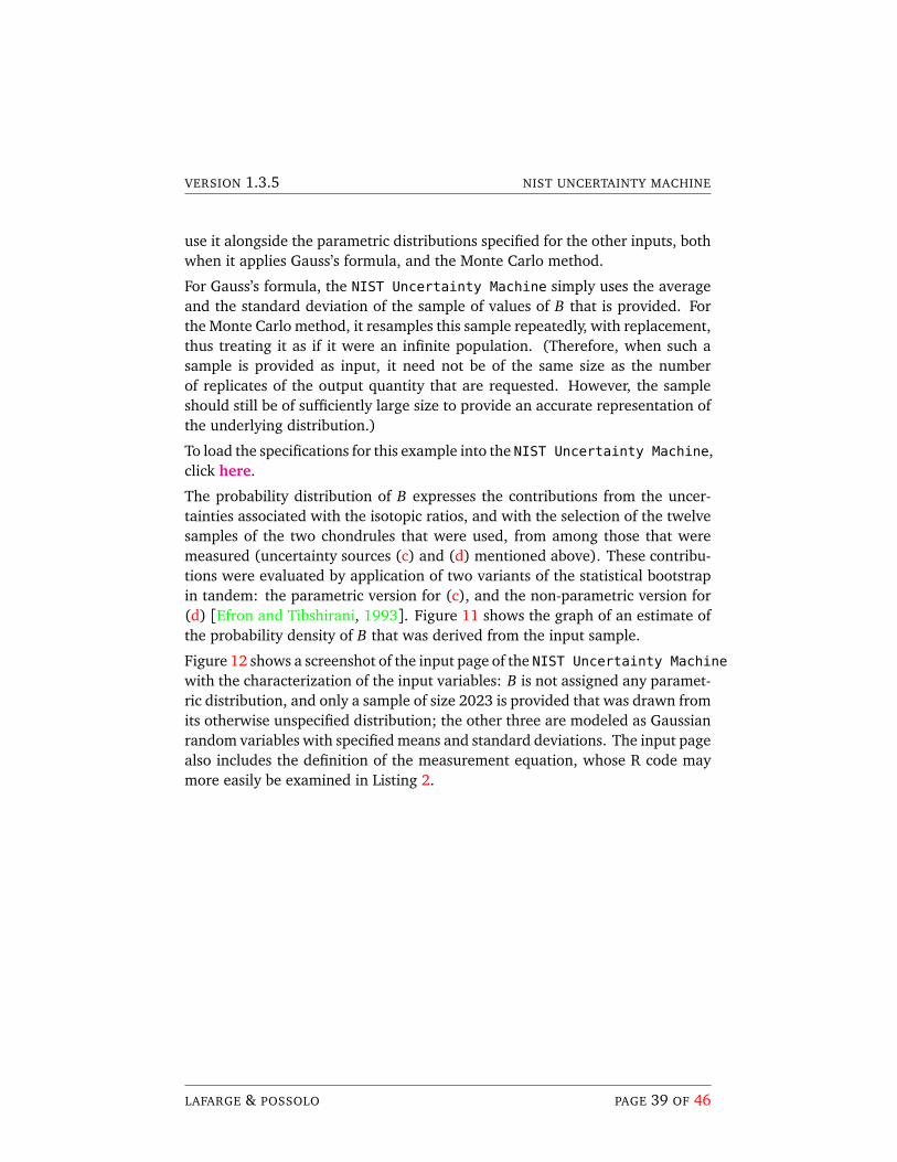
VERSION 1.3.5 NIST UNCERTAINTY MACHINE
use it alongside the parametric distributions specified for the other inputs, bothwhen it applies Gauss’s formula, and the Monte Carlo method.
For Gauss’s formula, the NIST Uncertainty Machine simply uses the averageand the standard deviation of the sample of values of B that is provided. Forthe Monte Carlo method, it resamples this sample repeatedly, with replacement,thus treating it as if it were an infinite population. (Therefore, when such asample is provided as input, it need not be of the same size as the numberof replicates of the output quantity that are requested. However, the sampleshould still be of sufficiently large size to provide an accurate representation ofthe underlying distribution.)
To load the specifications for this example into the NIST Uncertainty Machine,click here.
The probability distribution of B expresses the contributions from the uncer-tainties associated with the isotopic ratios, and with the selection of the twelvesamples of the two chondrules that were used, from among those that weremeasured (uncertainty sources (c) and (d) mentioned above). These contribu-tions were evaluated by application of two variants of the statistical bootstrapin tandem: the parametric version for (c), and the non-parametric version for(d) [Efron and Tibshirani, 1993]. Figure 11 shows the graph of an estimate ofthe probability density of B that was derived from the input sample.
Figure 12 shows a screenshot of the input page of the NIST Uncertainty Machine
with the characterization of the input variables: B is not assigned any paramet-ric distribution, and only a sample of size 2023 is provided that was drawn fromits otherwise unspecified distribution; the other three are modeled as Gaussianrandom variables with specified means and standard deviations. The input pagealso includes the definition of the measurement equation, whose R code maymore easily be examined in Listing 2.
LAFARGE & POSSOLO PAGE 39 OF 46
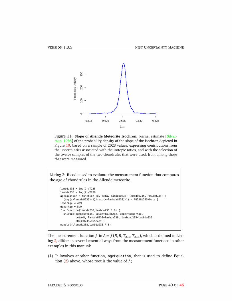
VERSION 1.3.5 NIST UNCERTAINTY MACHINE
0.615 0.620 0.625 0.630 0.635
010
020
030
0
βEIV
Pro
babi
lity
Den
sity
Figure 11: Slope of Allende Meteorite Isochron. Kernel estimate [Silver-man, 1986] of the probability density of the slope of the isochron depicted inFigure 10, based on a sample of 2023 values, expressing contributions fromthe uncertainties associated with the isotopic ratios, and with the selection ofthe twelve samples of the two chondrules that were used, from among thosethat were measured.
Listing 2: R code used to evaluate the measurement function that computesthe age of chondrules in the Allende meteorite.
lambda235 = log(2)/T235lambda238 = log(2)/T238ageEquation = function (x, beta, lambdaU238, lambdaU235, RU238U235) (exp(x*lambdaU235)-1)/(exp(x*lambdaU238)-1) - RU238U235*beta
lowerAge = 4e9upperAge = 5e9f = function(lambda238,lambda235,R,B) uniroot(ageEquation, lower=lowerAge, upper=upperAge,
beta=B, lambdaU238=lambda238, lambdaU235=lambda235,RU238U235=R)$root
mapply(f,lambda238,lambda235,R,B)
The measurement function f in A= f (B, R, T235, T238), which is defined in List-ing 2, differs in several essential ways from the measurement functions in otherexamples in this manual:
(1) It involves another function, ageEquation, that is used to define Equa-tion (2) above, whose root is the value of f ;
LAFARGE & POSSOLO PAGE 40 OF 46
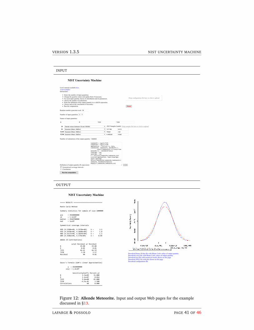
VERSION 1.3.5 NIST UNCERTAINTY MACHINE
INPUT
NIST Uncertainty Machine
User's manual available here.
Instructions :
Select the number of input quantities.Change the quantity names and update them if necessary.For each input quantity choose its distribution and its parameters.Choose the number of realizations.Write the definition of the output quantity in a valid R expression.Choose and set the correlations if necessary.Run the computation.
Drop configuration file here or click to upload
Reset
Random number generator seed: 54 Number of input quantities: 4
Names of input quantities:
B R T235 T238
B Sample values (between 30 and 100000) 2023 Samples loaded Drop sample file here or click to upload
R Gaussian (Mean, StdDev) 137.786 0.013
T235 Gaussian (Mean, StdDev) 704e6 1e6
T238 Gaussian (Mean, StdDev) 4.4683e9 4.8e6
Number of realizations of the output quantity: 1000000
Definition of output quantity (R expression):
lambda235 = log(2)/T235 lambda238 = log(2)/T238 ageEquation = function (x, beta, lambdaU238, lambdaU235, RU238U235) (exp(x*lambdaU235)-1)/(exp(x*lambdaU238)-1) - RU238U235*beta lowerAge = 4e9 upperAge = 5e9 f = function(lambda238,lambda235,R,B)uniroot(ageEquation, lower=lowerAge, upper=upperAge, beta=B,lambdaU238=lambda238,lambdaU235=lambda235, RU238U235=R)$root mapply(f,lambda238,lambda235,R,B)
- + Symmetrical coverage intervals Correlations
Run the computation
Load examples
OUTPUT
===== RESULTS ============================== Monte Carlo Method Summary statistics for sample of size 1000000 ave = 4568800000 sd = 1.1e+07 median = 4568700000 mad = 1e+07 Symmetrical coverage intervals 99% (4.5398e+09, 4.5978e+09) k = 2.5 95% (4.5478e+09, 4.5898e+09) k = 1.8 90% (4.5517e+09, 4.5859e+09) k = 1.5 68% (4.5586e+09, 4.579e+09) k = 0.89 ANOVA (% Contributions) w/out Residual w/ Residual B 29.80 29.80 R 0.01 0.01 T235 66.61 66.59 T238 3.58 3.57 Residual NA 0.02 -------------------------------------------- Gauss's Formula (GUM's Linear Approximation) y = 4568800000 u(y) = 1.2e+07 SensitivityCoeffs Percent.u2 B 2.3e+09 31.000 R 1.1e+07 0.014 T235 9.4e+00 65.000 T238 -4.5e-01 3.500 Correlations NA 0.000 ============================================
Download binary R data file with Monte Carlo values of output quantity Download a text file with Monte Carlo values of output quantity Download text file with numerical results shown on this page Download JPEG file with plot shown on this page Download configuration file
NIST Uncertainty Machine
Figure 12: Allende Meteorite. Input and output Web pages for the examplediscussed in §13.
LAFARGE & POSSOLO PAGE 41 OF 46
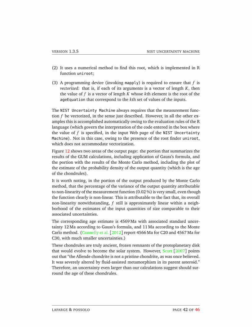
VERSION 1.3.5 NIST UNCERTAINTY MACHINE
(2) It uses a numerical method to find this root, which is implemented in Rfunction uniroot;
(3) A programming device (invoking mapply) is required to ensure that f isvectorized: that is, if each of its arguments is a vector of length K , thenthe value of f is a vector of length K whose kth element is the root of theageEquation that correspond to the kth set of values of the inputs.
The NIST Uncertainty Machine always requires that the measurement func-tion f be vectorized, in the sense just described. However, in all the other ex-amples this is accomplished automatically owing to the evaluation rules of the Rlanguage (which govern the interpretation of the code entered in the box wherethe value of f is specified, in the input Web page of the NIST Uncertainty
Machine). Not in this case, owing to the presence of the root finder uniroot,which does not accommodate vectorization.
Figure 12 shows two areas of the output page: the portion that summarizes theresults of the GUM calculations, including application of Gauss’s formula, andthe portion with the results of the Monte Carlo method, including the plot ofthe estimate of the probability density of the output quantity (which is the ageof the chondrules).
It is worth noting, in the portion of the output produced by the Monte Carlomethod, that the percentage of the variance of the output quantity attributableto non-linearity of the measurement function (0.02 %) is very small, even thoughthe function clearly is non-linear. This is attributable to the fact that, its overallnon-linearity notwithstanding, f still is approximately linear within a neigh-borhood of the estimates of the input quantities of size comparable to theirassociated uncertainties.
The corresponding age estimate is 4569 Ma with associated standard uncer-tainty 12 Ma according to Gauss’s formula, and 11 Ma according to the MonteCarlo method. (Connelly et al. [2012] report 4566 Ma for C20 and 4567 Ma forC30, with much smaller uncertainties.)
These chondrules are truly ancient, frozen remnants of the protoplanetary diskthat would evolve to become the solar system. However, Scott [2007] pointsout that “the Allende chondrite is not a pristine chondrite, as was once believed.It was severely altered by fluid-assisted metamorphism in its parent asteroid.”Therefore, an uncertainty even larger than our calculations suggest should sur-round the age of these chondrules.
LAFARGE & POSSOLO PAGE 42 OF 46

VERSION 1.3.5 NIST UNCERTAINTY MACHINE
Acknowledgments
The authors are grateful to their colleagues Will Guthrie, Alan Heckert, NarainKrishnamurthy, Adam Pintar, Jolene Splett, and Jack Wang, for the many sug-gestions that they offered for improvement of the NIST Uncertainty Machine
and of this user’s manual.
Alan Heckert, Steven Conn, Shawn Winhoven, Walter Rowe, Dale Little, andDel Brockett, greatly facilitated the deployment of this Web-based applicationfor use on the World Wide Web.
The authors will be very grateful to users of the software, and to readers of thismanual, for information about errors and other deficiencies, and for suggestionsfor improvement, which may be sent via eMail to [email protected]
and to [email protected].
References
T. W. Anderson and D. A. Darling. Asymptotic theory of certain “goodness-of-fit” criteriabased on stochastic processes. Annals of Mathematical Statistics, 23:193–212, 1952.
M.-M. Bé, V. Chisté, C. Dulieu, X. Mougeot, E. Browne, V. Chechev, N. Kuzmenco, F. Kon-dev, A. Luca, M. Galán, A. L. Nichols, A. Arinc, and X. Huang. Table of Radionuclides,volume 5 – A = 22 to 244 of Monographie BIPM-5. Bureau International des Poidset Mesures, Sèvres, France, 2010. ISBN 978-92-822-2234-8.
S. Bell. A Beginner’s Guide to Uncertainty of Measurement. Number 11 (Issue2) in Measurement Good Practice Guide. National Physical Laboratory, Tedding-ton, Middlesex, United Kingdom, 1999. URL www.npl.co.uk/publications/guides/a-beginners-guide-to-uncertainty-of-measurement. AmendmentsMarch 2001.
P. Billingsley. Probability and Measure. John Wiley & Sons, New York, NY, 1979.
R. S. Clarke, Jr., E. Jarosewich, B. Mason, J. Nelen, M. Gomez, and J. R. Hyde. Al-lende, Mexico, Meteorite Shower. Number 5 in Smithsonian Contributions to theEarth Sciences. Smithsonian Institution, Washington, DC, February 1971. doi:10.5479/si.00810274.5.1.
J. N. Connelly, M. Bizzarro, A. N. Krot, A. Nordlund, D. Wielandt, and M. A. Ivanova.The absolute chronology and thermal processing of solids in the solar protoplanetarydisk. Science, 338:651–655, November 2012. doi: 10.1126/science.1226919.
M. H. DeGroot and M. J. Schervish. Probability and Statistics. Addison-Wesley, 4thedition, 2011.
LAFARGE & POSSOLO PAGE 43 OF 46
VERSION 1.3.5 NIST UNCERTAINTY MACHINE
B. Efron and R. J. Tibshirani. An Introduction to the Bootstrap. Chapman & Hall, London,UK, 1993.
D. Freedman, R. Pisani, and R. Purves. Statistics. W. W. Norton & Company, New York,NY, fourth edition, 2007.
K. O. Friedrich. A Berry-Esseen bound for functions of independent random variables.The Annals of Statistics, 17(1):170–183, 1989.
C. Gauss. Theoria combinationis observationum erroribus minimis obnoxiae. In Werke,Band IV, Wahrscheinlichkeitsrechnung und Geometrie. Könighlichen Gesellschaft derWissenschaften, Göttingen, 1823. gdz.sub.uni-goettingen.de/.
P. Gilbert and R. Varadhan. numDeriv: Accurate Numerical Derivatives, 2016. URLCRAN.R-project.org/package=numDeriv. R package version 2016.8-1.
W. F. Guthrie, H.-k. Liu, A. L. Rukhin, B. Toman, J. C.M. Wang, and N.-f. Zhang. Threestatistical paradigms for the assessment and interpretation of measurement uncer-tainty. In F. Pavese and A. B. Forbes, editors, Data Modeling for Metrology and Testingin Measurement Science, Modeling and Simulation in Science, Engineering and Tech-nology, pages 1–45. Birkhäuser Boston, 2009. doi: 10.1007/978-0-8176-4804-6_3.
B. D. Hall and D. R. White. An Introduction to Measurement Uncertainty. Measure-ment Standards Laboratory of New Zealand, Lower Hutt, New Zealand, 2018. Alsoavailable from www.lulu.com.
J. Hiess, D. J. Condon, N. McLean, and S. R. Noble. 238U/235U systematics in terrestrialuranium-bearing minerals. Science, 335(6076):1610–1614, 2012. doi: 10.1126/science.1215507.
Joint Committee for Guides in Metrology. Evaluation of measurement data — Guide tothe expression of uncertainty in measurement. International Bureau of Weights andMeasures (BIPM), Sèvres, France, 2008a. URL www.bipm.org/en/publications/guides/gum.html. BIPM, IEC, IFCC, ILAC, ISO, IUPAC, IUPAP and OIML, JCGM100:2008, GUM 1995 with minor corrections.
Joint Committee for Guides in Metrology. Evaluation of measurement data — Supple-ment 1 to the “Guide to the expression of uncertainty in measurement” — Propagationof distributions using a Monte Carlo method. International Bureau of Weights andMeasures (BIPM), Sèvres, France, 2008b. URL www.bipm.org/en/publications/guides/gum.html. BIPM, IEC, IFCC, ILAC, ISO, IUPAC, IUPAP and OIML, JCGM101:2008.
Joint Committee for Guides in Metrology. Evaluation of measurement data — Supple-ment 2 to the “Guide to the expression of uncertainty in measurement” — Extensionto any number of output quantities. International Bureau of Weights and Measures(BIPM), Sèvres, France, 2011. URL www.bipm.org/en/publications/guides/gum.html. BIPM, IEC, IFCC, ILAC, ISO, IUPAC, IUPAP and OIML, JCGM 102:2011.
LAFARGE & POSSOLO PAGE 44 OF 46

VERSION 1.3.5 NIST UNCERTAINTY MACHINE
S. J. Kline and F. A. McClintock. Describing uncertainties in single-sample experiments.Mechanical Engineering, 75(1):3–8, 1953.
T. Lafarge and A. Possolo. The NIST Uncertainty Machine. NCSLI Measure Journal ofMeasurement Science, 10(3):20–27, September 2015.
P. J. Mohr, B. N. Taylor, and D. B. Newell. CODATA recommended values of the fun-damental physical constants: 2010. Reviews of Modern Physics, 84(4):1527–1605,October-December 2012. doi: 10.1063/1.4724320.
M. G. Morgan and M. Henrion. Uncertainty — A Guide to Dealing with Uncertainty inQuantitative Risk and Policy Analysis. Cambridge University Press, New York, NY, firstpaperback edition, 1992. 10th printing, 2007.
R. B. Nelsen. An Introduction to Copulas. Springer, New York, NY, 2nd edition, 2006.Corrected 2nd. printing, 2007.
D. B. Newell, F. Cabiati, J. Fischer, K. Fujii, S. G. Karshenboim, H. S. Margolis, E. de Mi-randés, P. J. Mohr, F. Nez, and K. Pachucki. The CODATA 2017 values of h, e, k,and NA for the revision of the SI. Metrologia, 55(1):L13–L16, January 2018. doi:10.1088/1681-7575/aa950a.
A. Possolo. Copulas for uncertainty analysis. Metrologia, 47:262–271, 2010. doi:10.1088/0026-1394/47/3/017.
A. Possolo. Simple Guide for Evaluating and Expressing the Uncertainty of NIST Mea-surement Results. National Institute of Standards and Technology, Gaithersburg,MD, 2015. URL http://dx.doi.org/10.6028/NIST.TN.1900. NIST Technical Note1900.
A. Possolo and C. Elster. Evaluating the uncertainty of input quantities in measurementmodels. Metrologia, 51(3):339–353, June 2014. doi: 10.1088/0026-1394/51/3/339.
A. Possolo and H. K. Iyer. Concepts and tools for the evaluation of measurement un-certainty. Review of Scientific Instruments, 88(1):011301, 2017. doi: 10.1063/1.4974274.
A. Possolo, B. Toman, and T. Estler. Contribution to a conversation about the Supple-ment 1 to the GUM. Metrologia, 46:L1–L7, 2009.
R Core Team. R: A Language and Environment for Statistical Computing. R Foundationfor Statistical Computing, Vienna, Austria, 2015. URL www.R-project.org/.
F. E. Satterthwaite. An approximate distribution of estimates of variance components.Biometrics Bulletin, 2(6):110–114, December 1946.
LAFARGE & POSSOLO PAGE 45 OF 46
VERSION 1.3.5 NIST UNCERTAINTY MACHINE
B. Schoene. U-Th-Pb Geochronology. In H. D. Holland and K. K. Turekian, editors,Treatise on Geochemistry, volume 4 (The Crust), chapter 10, pages 341–378. Elsevier,Amsterdam, second edition, 2014. doi: 10.1016/B978-0-08-095975-7.00310-7.
E. R. D. Scott. Chondrites and the protoplanetary disk. Annual Review of Earth and Plan-etary Sciences, 35:577–620, 2007. doi: 10.1146/annurev.earth.35.031306.140100.
B. W. Silverman. Density Estimation. Chapman and Hall, London, 1986.
B. N. Taylor and C. E. Kuyatt. Guidelines for Evaluating and Expressing the Uncertaintyof NIST Measurement Results. NIST Technical Note 1297. National Institute of Stan-dards and Technology, Gaithersburg, MD, 1994. URL physics.nist.gov/Pubs/guidelines/TN1297/tn1297s.pdf.
C. M. Tsui, A. Y. K. Yang, and H. W. Li. Software tools for evaluation of measurementmodels for complex-valued quantities in accordance with Supplement 2 to the GUM.NCSLI Measure Journal of Measurement Science, 7(3):48–55, September 2012.
I. M. Villa, M. L. Bonardi, P. De Bièvre, N. E. Holden, and P. R. Renne. IUPAC-IUGSstatus report on the half-lives of 238U, 235U and 234U. Geochimica et CosmochimicaActa, 172:387–392, 2016. doi: 10.1016/j.gca.2015.10.011.
B. L. Welch. The generalization of ‘Student’s’ problem when several different populationvariances are involved. Biometrika, 34:28–35, January 1947.
W. M. White. Isotope Geochemistry. John Wiley & Sons, New York, NY, 2015.
LAFARGE & POSSOLO PAGE 46 OF 46