Nicolas Berman, Philippe Martin and Thierry Mayer

How do different exporters

react to exchange-rate

changes? Theory, empirics

and aggregate implications

EFIGE working paper 20

November 2009

Previously published in the CEPR Discussion Paper Series No.7493

Nicolas Berman, Philippe Martin and Thierry Mayer

EFIGE IS A PROJECT DESIGNED TO HELP IDENTIFY THE INTERNAL POLICIES NEEDED TO IMPROVE EUROPE’S EXTERNAL COMPETITIVENESS

Funded under the

Socio-economic

Sciences and

Humanities

Programme of the

Seventh

Framework

Programme of the

European Union.

LEGAL NOTICE: The

research leading to these

results has received

funding from the

European Community's

Seventh Framework

Programme (FP7/2007-

2013) under grant

agreement n° 225551.

The views expressed in

this publication are the

sole responsibility of the

authors and do not

necessarily reflect the

views of the European

Commission.

The EFIGE project is coordinated by Bruegel and involves the following partner organisations: Universidad Carlos III de Madrid, Centre forEconomic Policy Research (CEPR), Institute of Economics Hungarian Academy of Sciences (IEHAS), Institut für Angewandte Wirtschafts-forschung (IAW), Centro Studi Luca D'Agliano (Ld’A), Unitcredit Group, Centre d’Etudes Prospectives et d’Informations Internationales (CEPII).The EFIGE partners also work together with the following associate partners: Banque de France, Banco de España, Banca d’Italia, DeutscheBundesbank, National Bank of Belgium, OECD Economics Department.

DISCUSSION PAPER SERIES

ABCD

www.cepr.org

Available online at: www.cepr.org/pubs/dps/DP7493.asp www.ssrn.com/xxx/xxx/xxx

No. 7493

HOW DO DIFFERENT EXPORTERS REACT TO EXCHANGE RATE

CHANGES? THEORY, EMPIRICS AND AGGREGATE IMPLICATIONS

Nicolas Berman, Philippe Martin and Thierry Mayer

INTERNATIONAL MACROECONOMICS and INTERNATIONAL TRADE AND

REGIONAL ECONOMICS

ISSN 0265-8003

HOW DO DIFFERENT EXPORTERS REACT TO EXCHANGE RATE

CHANGES? THEORY, EMPIRICS AND AGGREGATE IMPLICATIONS

Nicolas Berman, Graduate Institute of International and Development Studies Philippe Martin, Sciences Po, Paris and CEPR

Thierry Mayer, Sciences Po, Paris, CEPII and CEPR

Discussion Paper No. 7493 October 2009

Centre for Economic Policy Research 53–56 Gt Sutton St, London EC1V 0DG, UK

Tel: (44 20) 7183 8801, Fax: (44 20) 7183 8820 Email: [email protected], Website: www.cepr.org

This Discussion Paper is issued under the auspices of the Centre’s research programme in INTERNATIONAL MACROECONOMICS and INTERNATIONAL TRADE AND REGIONAL ECONOMICS. Any opinions expressed here are those of the author(s) and not those of the Centre for Economic Policy Research. Research disseminated by CEPR may include views on policy, but the Centre itself takes no institutional policy positions.

The Centre for Economic Policy Research was established in 1983 as an educational charity, to promote independent analysis and public discussion of open economies and the relations among them. It is pluralist and non-partisan, bringing economic research to bear on the analysis of medium- and long-run policy questions.

These Discussion Papers often represent preliminary or incomplete work, circulated to encourage discussion and comment. Citation and use of such a paper should take account of its provisional character.

Copyright: Nicolas Berman, Philippe Martin and Thierry Mayer

CEPR Discussion Paper No. 7493

October 2009

ABSTRACT

How do different exporters react to exchange rate changes? Theory, empirics and aggregate implications

This paper analyzes the reaction of exporters to exchange rate changes. We present a model where, in the presence of distribution costs in the export market, high and low productivity firms react differently to a depreciation . Whereas high productivity firms optimally raise their markup rather than the volume they export, low productivity firms choose the opposite strategy. Hence, pricing to market is both endogenous and heterogenous. This heterogeneity has important consequences for the aggregate impact of exchange rate movements. The presence of fixed costs to export means that only high productivity firms can export, firms which precisely react to an exchange rate depreciation by increasing their export price rather than their sales. We show that this selection effect can explain the weak impact of exchange rate movements on aggregate export volumes. We then test the main predictions of the model on a very rich French firm level data set with destination-specific export values and volumes on the period 1995-2005. Our results confirm that high performance firms react to a depreciation by increasing their export price rather than their export volume. The reverse is true for low productivity exporters. Pricing to market by exporters is also more pervasive in sectors and destination countries with higher distribution costs. Consistent with our theoretical framework, we show that the probability of firms to enter the export market following a depreciation increases. The extensive margin response to exchange rate changes is modest at the aggregate level because firms that enter, following a depreciation, are smaller relative to existing firms.

JEL Classification: F12 and F41 Keywords: distribution costs, exchange rates, exports, heterogeneity, pricing to market and productivity

Nicolas Berman Graduate Institute of International and Development Studies Case Postale 136 CH - 1211 Genève SWITZERLAND Email: [email protected] For further Discussion Papers by this author see: www.cepr.org/pubs/new-dps/dplist.asp?authorid=166315

Philippe Martin Sciences Po 27, Rue Saint-Guillaume 75007 Paris FRANCE Email: [email protected] For further Discussion Papers by this author see: www.cepr.org/pubs/new-dps/dplist.asp?authorid=116056

Thierry Mayer Sciences Po 27, Rue Saint-Guillaume 75007 Paris FRANCE Email: [email protected] For further Discussion Papers by this author see: www.cepr.org/pubs/new-dps/dplist.asp?authorid=152707

*This paper is produced as part of the project European Firms in a Global Economy: Internal policies for external competitiveness (EFIGE), a Collaborative Project funded by the European Commission's Seventh Research Framework Programme, Contract number 225551.

We thank Anders Akerman, Andrew Atkeson, Ariel Burstein, Giancarlo Corsetti, Mario Crucini, Linda Goldberg, Samuel Kortum, Francis Kramarz, Steve Redding David Weinstein and participants at the Federal Reserve Bank of New York, Sciences-Po, CREST-LMA, Oslo university, Cesifo Summer Institute, Banco de Portugal, Bank of Hungary, Berkeley, UCLA, Federal Reserve Bank of San Francisco, University Nova of Lisbon and AEA, NBER Summer Institute and ERWIT Meetings for helpful comments. We are very grateful to Linda Goldberg who provided us the data on distribution costs. Philippe Martin and Thierry Mayer thank the Institut Universitaire de France for financial help. Submitted 07 October 2009

Abstract

This paper analyzes the reaction of exporters to exchange rate changes. We present a model

where, in the presence of distribution costs in the export market, high and low produc-

tivity firms react differently to a depreciation . Whereas high productivity firms optimally

raise their markup rather than the volume they export, low productivity firms choose the

opposite strategy. Hence, pricing to market is both endogenous and heteroegenous. This

heterogeneity has important consequences for the aggregate impact of exchange rate move-

ments. The presence of fixed costs to export means that only high productivity firms can

export, firms which precisely react to an exchange rate depreciation by increasing their ex-

port price rather than their sales. We show that this selection effect can explain the weak

impact of exchange rate movements on aggregate export volumes. We then test the main

predictions of the model on a very rich French firm level data set with destination-specific

export values and volumes on the period 1995-2005. Our results confirm that high perfor-

mance firms react to a depreciation by increasing their export price rather than their export

volume. The reverse is true for low productivity exporters. Pricing to market by exporters

is also more pervasive in sectors and destination countries with higher distribution costs.

Consistent with our theoretical framework, we show that the probability of firms to enter

the export market following a depreciation increases. The extensive margin response to ex-

change rate changes is modest at the aggregate level because firms that enter, following a

depreciation, are smaller relative to existing firms.

1 Introduction

Movements of nominal and real exchange rates are large. They however seem to have little

effect on aggregate variables such as import prices, consumer prices, and the volumes of

imports and exports. The sensitivity, or rather lack of, of prices to exchange rate movements

has been well documented by Goldberg and Knetter (1997) and Campa and Goldberg (2005

and 2008) who provide estimates of the pass-through of exchange rates into import prices.

There is also evidence indicating a decline in exchange rate pass-through to import prices

in the U.S. On the quantity side, the elasticity of aggregate exports to real exchange rate

movements is typically found to be low in industrialized countries, a bit below unity for

example in Hooper, Johnson, and Marquez (2000) and above unity but rarely above 2 in

others studies. In international real business cycle models, the elasticity used for simulations

is typically between 0.5 and 2.

One possible explanation is that prices are rigid in the currency of the export market.

However, Campa and Goldberg, (2005) show that the incomplete pass-through of exchange

rate changes into import prices is far from being a short-term phenomenon as it remains

after one year. This suggests that price rigidities cannot fully explain this phenomenon.

Moreover, Gopinath and Rigobon (2008) have recently shown on good-level data, that even

conditioning on a price change, trade weighted exchange rate pass-through into U.S. import

prices is low, at 22%. Another explanation is the presence of local distribution costs. These

can directly explain why consumer prices do not respond fully to exchange rate movements.

Corsetti and Dedola (2007) show that with imperfect competition, distribution costs may

also explain why import prices themselves do not respond much to exchange rate movements.

In this paper, we show that the heterogeneity of the optimal response of exporters to

exchange rate movements can help explain the lack of response of aggregate variables (prices

and quantities) to these movements. We show theoretically and empirically that high and

low performance firms react very differently to exchange rate movements. We interpret

performance in terms of productivity or, in an alternative version of the model, in terms

of quality. Whereas, following a depreciation, high performance firms optimally raise their

markup rather than the volume they export, low performance firms choose the opposite

strategy. Another way to state this result is that high performance firms absorb exchange

rate movements in their markups but low performance firms do not. The reason is that,

due to local distribution costs, the demand elasticity perceived by high performance firms

is lower than the elasticity perceived by low performance ones. This heterogeneity is a novel

finding and is also interesting because of its implications for aggregate effects of exchange

1

rate movements. In our model, following the spirit of Melitz (2003), fixed export costs

generate a selection mechanism through which only the best performers are able to export.

Also, heterogeneity in productivity implies that a very large share of aggregate exports is

made by a small portion of high performance firms. Hence, exporters, and even more so big

exporters, are, by this selection effect, firms which optimally choose to absorb exchange rate

movements in their markups. A depreciation also leads new firms to enter the export market

but these are less productive and smaller than existing ones. We show that our model, with

sufficient heterogeneity in productivity, can indeed reproduce the observed low level of the

elasticity of the intensive and extensive margins of trade to exchange rate movements.

The model produces testable implications on the heterogeneity of the sensitivity of firm

level export prices and volumes to exchange rates. We test these predictions on a very rich

firm-level dataset. We collected information on firm-level, destination-specific export values

and volumes from the French Customs and other information on firm performance at annual

frequency. This is the same source as the one used by Eaton, Kortum, and Kramarz (2008)

for the year 1986. We use this data set for a longer and more recent period (1995-2005)

so that we can exploit variation across both years and destinations1. To our knowledge,

our paper is the first to exploit such detailed data to document the reaction of firms to

exchange rate movements in terms of prices, quantities, entry and exit and to analyze how

different firms react differently to exchange rate movements. A big advantage of our dataset

is that we have information that can proxy for the FOB price at the producer/destination

level. We can infer the impact of a depreciation on the pricing strategy of the exporter.

Our paper is therefore complementary to existing studies on pricing to market and pass-

through which use information that proxies pricing strategies of exporters through import

prices2 (which contain transport costs) or consumer prices3 (which also contain distribution

costs). We first show that firms with performance (measured by TFP, labor productivity,

export size, number of destinations) above the median react to a 10% depreciation by

increasing their (destination specific) export price in euro by around 2%. In contrast, those

firms below median performance do not change export prices in reaction to a change in

exchange rate. Hence, only high performance partially price to market and partially absorb

exchange rate movements in their mark-ups. On export volumes (again destination specific),

the reverse is true: for the best performers export volumes do not react to exchange rate

1Berthou and Fontagné (2008a, and b) use this same data set to analyze the effect of the creation of the

euro on the exports of French firms.

2 See for example Gopinath and Itskhoki (2008), Gopinath, Itskhoki and Rigobon (2009), Halpern and

Koren (2008).

3 See Crucini and Shintani (2008) and Gopinath, Gourinchas, Hsieh and Li (2009) for example.

2

movements but poor performers react by increasing their export volumes by around 6%.

We also find that, following a depreciation, French exporters selling in sectors and countries

with high distribution costs, choose to increase their mark-up rather than their export

volumes. Distribution costs in the destination market therefore change the pricing strategy

of exporters towards more pricing to market. Again, this is consistent with our theoretical

framework and with the model of Corsetti and Dedola (2007).

To our knowledge, our paper is also the first to document the impact of exchange rate

changes on entry and exit in different destinations. The model predicts entry of firms follow-

ing a depreciation4 We find that this is indeed the case for French firms and, surprisingly,

that this entry takes place relatively quickly, within a year. The extensive margin represents

around 20% of the total increase in exports. However, because the new entrants are on

average smaller than existing exporters, the extensive margin of exchange rate movements

on exports has a limited effect at the aggregate level.

Consistently with the existing literature, we find that the aggregate elasticity of exports

to exchange rate is low, a little bit above unity. We show that with sufficient heterogeneity

and plausible distribution costs margins, our model, in the absence of nominal rigidities,

can reproduce the observed low aggregate elasticities at both the intensive and extensive

margins. Empirically, and consistent with the key role of heterogeneity in our model, we

also find that sectors with more heterogenous firms are those for which aggregate export

volumes are the least sensitive to exchange rate movements.

At the origin of our results is the interaction between two key elements recently em-

phasized by the international trade and macroeconomics literatures. The first element is

productivity heterogeneity across firms which has been theoretically analyzed by Melitz

(2003) and Chaney (2008) in the trade context. Several papers have documented the fact

that firms that export have higher productivity and perform better than other firms more

generally (see for the French case, Eaton, Kortum, and Kramarz (2004 and 2008)). This

is due to the existence of fixed costs of exports that allows only high performers to export.

Moreover, a very large share of exports is concentrated on a small number of firms, the

best performers among the exporters (see Bernard, Jensen, Redding and Schott 2007 and

Mayer and Ottaviano, 2007). The second element is local distributions costs that have to

be paid by firms to reach consumers. Evidence of the significance of these costs have been

found by Goldberg and Campa (2008) and previously emphasized by Anderson and Van

Wincoop (2004) among others; they are generally found to constitute a 40 to 60 percent

4Bernard, Eaton, Jensen and Kortum (2003), in a theoretical model with firm heterogeneity, entry and

exit find that an appreciation leads some of the firms to stop exporting.

3

share of consumer prices. Burstein, Neves, and Rebelo (2003) report that distribution costs

represent more than 40 percent of the retail price in the US and 60 percent of the retail

price in Argentina. We show in this paper that the interaction of firms’ heterogeneity and

local distribution costs generate heterogenous optimal response to exchange rate changes in

terms of prices (heterogenous pricing to market) and quantities.

Our paper is related to the literature on incomplete exchange rate pass-through and

pricing to market. A recent paper by Auer and Chaney (2008) shows that the pass-through

can be incomplete and heterogeneous across goods of different quality in a model with

heterogenous consumers. Our paper is also related to the papers (Corsetti and Dedola, 2007

and Atkeson and Burstein, 2008) which have analyzed the impact of distribution costs on

the extent of the pass-through. Indeed, in our model, local distribution costs directly lower

the pass-through to consumer prices but also generate variable producer mark-ups as in

Corsetti and Dedola (2007) that further reduce the pass-through.

Burstein, Neves, and Rebelo (2003) analyze the role of nontradable distribution costs in

accounting for the behavior of international relative prices. and show that because distribu-

tion services require local labor, they drive a natural wedge between retail prices in different

countries. Burstein, Eichenbaum, and Rebelo (2005) show that distribution costs are also

key to understand the large drop in real exchange rates that occurs after large devaluations.

In the theoretical contribution of Atkeson and Burstein (2008), distribution costs also play

an important role to explain deviations from relative purchasing power parity in a model

with imperfect competition and variable markups. The model they present is the closest

to ours because they show that in the presence of trade costs and imperfect competition

large firms have an incentive to price to market. Hence, heterogeneity across firms features

prominently in their analysis of pricing to market and deviations from PPP. Different from

Atkeson and Burstein (2008), we focus on both prices and quantities and the mechanism

we analyze in our theoretical contribution depends on the interaction between heterogeneity

in productivity and local distribution costs. In addition, we test our predictions on a very

detailed firm-level dataset for both prices and quantities. Our empirical results on prices are

consistent with several aspects of their theoretical model, in particular the fact that firms

differ in the degree to which they price to market and that this heterogeneity may have

important aggregate consequences. Two other related papers are Dekle, Jeong and Ryoo

(2007) and Imbs and Mejean (2009) who show that the aggregation of heterogenous firms

or sectors can result into an aggregation bias in the estimation of the elasticity of exports

to exchange rate changes. Their firm and sector level analysis concludes that estimates of

the elasticity parameter at the firm or sector and at the (consistently) aggregated levels are

4

similar.

There are few empirical contributions on pricing to market, exchange rate and export

flows using exporter-level data5. Martin and Rodriguez (2004) find that Spanish firms do

react to a depreciation by raising their mark up. Hellerstein (2008) uses a detailed dataset

with retail and wholesale prices for beer and finds that markup adjustments by manufac-

turers and retailers explain roughly half of the incomplete pass-through whereas local costs

components account for the other half. Gaulier, Lahrèche-Révil and Méjean (2006) show,

using product-level data, that pricing to market is more pervasive when the goods are traded

on referenced markets and for final consumption goods. Their study stresses strong hetero-

geneity in pricing to market across products. Bernard, Jensen an Schott (2006) show that

multinationals differentially adjust their prices inside and outside the firm in response to

exchange rate movements. Fitzgerald and Haller (2008) use an Irish firm level data set and

show that, conditioning on goods being invoiced in destination currency and observing a

price change, mark-ups move one-for-one with movements of the exchange rate. However,

these studies do not analyze how and why different firms react differently to an exchange

rate movement and how their sales and entry/exit decision are affected which is the focus of

our paper. Using British data, Greenaway, Kneller and Zhang (2007) analyze the exporter

status choice following exchange rate variations but they do not have information on export

destination, nor on the pricing strategy of firms.

The paper is organized as follows. We derive the main theoretical results and predictions

in the next section. Section 3 presents the data set, the empirical methodology and the main

findings. Section 4 concludes.

2 Theoretical framework

2.1 Preferences and technology

We analyze a simple model in which heterogenous firms of a country (called Home) export

to countries. The aim is to derive testable implications concerning the impact of ex-

change rate movements on exporters behavior. In the empirical section, where we test those

5Other papers analyze different aspects of firms reactions to exchange rate shocks. Gourinchas (1999),

evaluates the impact of exchange rate fluctuations on inter- and intra-sectoral job reallocation. The pa-

per investigates empirically the pattern of job creation and destruction in response to real exchange rate

movements in France between 1984 and 1992, using disaggregated firm-level data and finds that traded-

sector industries are very responsive to real exchange rate movements. Ekholm, Moxnes and Ullveit-Moe

(2008) study firms’ response to the appreciation of the Norwegian Krone in the early 2000s with respect to

employment, productivity, and offshoring.

5

implications, the exporter country will be France. For notational simplicity, given that we

concentrate on one exporter country (Home), we drop subscripts that describe this country.

There is only one sector which operates under monopolistic competition.

The origin of the movements in the bilateral real exchange rates with each countries

will be left exogenous but could be made endogenous either by introducing monetary shocks

that move the nominal exchange rate under the assumption of rigid nominal wages or pro-

ductivity shocks in a non tradeable sector. Corsetti and Dedola (2007) analyze both in a

general equilibrium model. Ghironi and Melitz (2005) and Atkeson and Burstein (2008)

focus on productivity shocks. We prefer to remain agnostic on the origin of real exchange

rate movements in short-medium term horizon (around one year) on which we will focus

in the empirical section. One reason is the failure of the empirical literature to find an im-

portant role for fundamentals (monetary or real) to real exchange rate movements on this

horizon. Another is that one aim of our model is to derive testable implications of the effect

of exchange rate movements at the firm level, a level at which we can take these movements

as exogenous.

Utility for a representative agent in country is derived from consumption of a continuum

of differentiated varieties in the standard Dixit-Stiglitz framework:

() =

⎡⎣Z

()1−1

⎤⎦ 11−1

(1)

where () is the consumption of variety . Firms are indexed by which represents their

productivity (1 is the number of units of labor necessary for producing the good). As will

be seen below, also affects the fixed cost of production in the country where the firm is

located. The set of traded varieties is . The elasticity of substitution between two varieties

is 1

We assume that several trade costs impede transactions at the international level: an

iceberg trade cost, a fixed cost of exporting and a distribution cost.

First, we assume an iceberg trade cost 1 between Home and country , the desti-

nation country. units of the good are produced and shipped but only one unit arrives at

destination.

Second, in order to export in country , a firm producing in the Home country must pay

a fixed cost, specific to each destination (). We will characterize the specific form of this

fixed cost when we analyze the effect of exchange rates on the extensive margin of trade as

this specific form does not affect the intensive margin of trade.

Finally, we assume that distribution (wholesale and retail) costs have to be paid in the

6

destination country on the amount that reaches the destination. Distribution takes units

of labor in country per unit consumed in that country. Hence, we follow Tirole (1995), (p.

175) characterization of distribution: "production and retailing are complements". This

is the same assumption as in Burstein, Neves and Rebelo (2003) and Corsetti and Dedola

(2007). The wage paid in distribution is the same as in the production sector. We assume that

the cost of distribution does not depend on the idiosyncratic productivity of the firm. Again,

this means that the distribution costs are outsourced. Those costs are paid to an outside firm

that provides distribution services. If a French firm exports to the US, we therefore assume

that what it pays in distribution services (to wholesalers and retailers) does not depend

on its productivity. Any additive cost (transport, marketing, advertising, insurance...) -

not substitutable to production - paid in local currency and which does not depend on the

productivity of the exporter would have the same impact as the distribution costs we assume

here. Qualitatively, our results would remain if these distribution costs depended on the

firm’s productivity, as long as they react less to productivity than production costs.

In our model, the costs that depend directly on productivity are at the core of what

defines a firm and a product: these are the production costs and the share of the fixed cost

of exporting that is borne in the country where the firm is located.

In units of currency of country , the consumer price () of a variety exported from

Home to country is:

() ≡()

+ (2)

where () is the producer price of the good exported to expressed in Home currency.

is the wage rate in country and is the nominal exchange rate between the Home

country and country expressed as Home currency in units of currency. An increase in

is a depreciation in the Home currency vis a vis currency . The quantity demanded in of

this variety is:

() = −1 [ ()]

−(3)

where is the income of country and is the price index in country . The cost

(in units of currency of the Home country) of producing () units of good (inclusive of

transaction costs) and selling them in country for a domestic firm with productivity is:

() = () + () (4)

where is the wage rate in the Home country. will be more generally interpreted as a

measure of the performance of the firm that can affect its sales and its presence on markets.

7

The profits (in units of currency of the Home country) of exporting this variety to country

are therefore given by:

() = [()− ]() − () (5)

2.2 Prices and the intensive margin

With monopolistic competition on the production side, the producer price () expressed

in Home currency of firm/variety exporting to country is higher than −1 , the standard

mark-up in the monopolistic competition model:

() =

− 1µ1 +

¶

= ()

(6)

where we call ≡ the real exchange rate of the Home country with country .

The mark-up () over the marginal cost increases with the productivity of the firm and

the exchange rate6. Due to high productivity and low producer prices, a large share of the

final consumer price does not depend on the producer price so that the elasticity of demand

perceived by the producer is lower. The producer price can be rewritten as a function of

this perceived elasticity () :

() =()

()− 1

where () =

+

+ 1 (7)

() is lower than , the elasticity in the standard monopolistic competition model. High

productivity firms (high ) have a lower elasticity which explains their higher mark-up. A

depreciation (higher ) also reduces the perceived demand elasticity which allows all firms

to increase their markup. High productivity firms, because they have a lower elasticity to

start with, can increase their markup more than others.

Note that the law of one price does not hold: the producer price of the same variety sold

in different countries depends on the bilateral exchange rate, trade and distribution costs

and the wage rate of this country. The impact of a depreciation on the producer price is

given by the following elasticity, specific to each firm:

() =()

()=

+ (8)

6Bergin and Feenstra. (2000, 2001, 2009) show that producer mark-ups also increase with a depreciation

in a model with translog preferences. Atkeson and Burstein (2008) show the same result in a model with

quantity competition à la Cournot. In a model with decreasing returns to labor rather than the linear

production function we assume, firms would also react to a depreciation by increasing producer prices. This

is because their marginal costs increase with production. However, in the absence of distribution costs, the

elasticity of the producer price to exchange rate would not depend on productivity.

8

Testable Prediction 1. The elasticity of the producer price, () to a real depreciation

(an increase in ) is positive and

i) increases with the productivity of the firm , the size of its exports and more generally

its performance on exports markets.

ii) increases with the importance of local distribution costs

iii) increases with the level of the real exchange rate

The mark-up increases with a depreciation because distribution costs involve some en-

dogenous pricing to market as explained by Corsetti and Dedola (2007). Firms partially

absorb some of the exchange rate change in the mark-up. (), which can be thought as a

measure of pricing to market, which here is heterogenous and increases with the productiv-

ity of the exporter. The productivity of a firm affects positively the size of its exports and

the number of markets it exports to (see below). Hence, the elasticity of the producer price

to a real depreciation should increase with these measures of export performance. These

predictions also hold in a version of the model presented in appendix in which firms differ

in the quality of the goods they export. In this case, firms that export higher quality goods

(and have higher value added per worker) react to a depreciation by a larger increase of

their producer price.

Firms that export in countries and sectors with higher distribution costs should react to

a real depreciation by increasing more their producer prices. This is because the elasticity

of demand perceived by the producer is lower on those markets.

Finally, the reason for prediction (iii) is that the share of the price affected by the

exchange rate decreases with the exchange rate itself. In fact, a depreciation acts as a

productivity gain for all firms and — exactly as a productivity gain — it increases the share

of the distribution costs in consumer prices and reduces the elasticity of demand perceived

by the producer. The effect of a real depreciation is therefore non linear.

The import price and the consumer price (expressed in the currency of country ) are:

() =()

=

− 1µ

+

¶; () =

− 1µ

+

¶(9)

so that there is incomplete pass-through of a depreciation at the level of both import

and consumer prices. Part of the lack of response of the consumer price to exchange rate

comes directly from the presence of local distribution costs and part comes from the change

in the mark-up of the producer as a response to the exchange rate change7. The optimal

degree of pass-through on prices at the import and consumer levels are respectively:

7Hellerstein (2008) work on the beer market estimates that half of the lack of complete pass-through in

this market is due to changes in mark-up and half to local distribution costs.

9

()

()= −

+ ; ()

()= −

+ (10)

and decreases with both the importance of the distribution cost and the productivity of the

firm. Note that in our model, we do not consider the choice of currency of invoicing but

the optimal choice of the degree of pass-through is implicitly similar to such a choice. If the

elasticity in (10) for both the import and consumer price approaches -1, this is similar to

producer currency pricing. At the other extreme, if it approaches zero (for example, for very

high productivity firms and or distribution costs), this is similar to local currency pricing.

For an active exporter, the volume of exports increases with productivity:

() = −1

∙

+

¸−−

µ − 1

¶(11)

where is the ideal price index in country :

=

ÃX=1

Z ∞∗

h

− 1³ +

´i1−()

!−1(−1)(12)

where is the bilateral real exchange rate of country and and the bilateral

trade cost. Note that as in Chaney (2008), we assume that the number of entrepreneurs

who get a productivity draw is proportional to the population size in country Only

firms with productivity above ∗ in country can export in country . Note that the

price index for country depends on the bilateral exchange rates of country with all its

trade partners. In this perfect price index, a measure of the effective real exchange rate of

the country appears in the second part of the bracket (in a very non linear way). More

precisely, it is the weighted sum of real bilateral exchange rates of country with all its

trading partners. The weights depend in particular on the number of exporters which is

proportional to the number of workers. Hence an effective exchange rate appreciation of

country that decreases leads to a fall of the volume of exports from an exporter of the

Home country. We will assume that the Home country is too small for its bilateral exchange

rate to affect the price index of country .

We can now analyze the impact of a change in the bilateral real exchange rate on the

volume of exports between the Home country and country , characterized by the following

elasticity, specific to each firm:

() =()

()=

+ (13)

10

Testable Prediction 2. The elasticity of the firm exports, () to a real depreciation

(an increase in ) is positive and

i) decreases with the productivity of the firm , the size of its exports and more generally

its performance on exports markets

ii) decreases with the importance of local distribution costs

iii) decreases with the level of the real exchange rate

The intuition of these predictions on export volumes comes directly from the intuition on

producer prices. Heterogenous absorption of real exchange rate movements into mark-ups

generates an heterogenous reaction of export volumes. Again, these results hold in a version

of the model presented in appendix in which firms differ in the quality of the goods they

export.

The elasticity of the value of exports (in Home currency) to exchange rate change of a

firm with productivity is the sum of the elasticities given in (8) and (13). It can be checked

that the elasticity of the value of exports to decreases with the productivity of the firm

as long as 1 i.e. the relevant case in our model.

2.3 Profits and the extensive margin

The equilibrium profits for an active Home country exporter to country can be shown to be:

() =

()()

− () (14)

= −

−1

∙

+

¸1−− ()

where ≡ −( − 1)−1 is a constant. We now specify the fixed export cost (). Weassume that workers in both countries are employed to pay this fixed cost which might be

interpreted as research and development, innovation, adaptation to the market or marketing

expenses. We assume that firms with higher productivity in production activities are also

more productive in activities (R&D, innovation, marketing expenses...) necessary to provide

the fixed cost. The production function for the fixed cost to export is more general than

in the existing literature because we allow for it to be partly incurred in the destination

country, for example in the case of marketing costs. It is expressed as a Cobb-Douglas in

labor of the Home country and labor in country , with shares and 1− respectively:

() =

µ

¶()

1−=

−1− (15)

where 0 This specification implies that the productivity parameter that characterizes

the firm affects its fixed cost only in the country where production is located. Implicitly,

this means that the share of fixed costs paid in the foreign country is outsourced.

11

One can show that profits increase with a real depreciation. Partly this is because sales

increase in country and partly this is because the mark-up of exporting to country

increases with the depreciation.

The threshold such that profits of a firm ∗ exporting in are zero is (implicitly) defined

by the following cutoff condition:

− −1

∙

∗+

¸1−= (

∗)−

(16)

Below the threshold productivity ∗ , firms are not able to export on market . Exporters are

higher productivity firms as in Melitz (2003). Given that we showed in the previous section

that higher productivity firms choose to absorb more of the exchange rate movements into

their mark-up, this implies that exporters are firms which, by selection, are less sensitive

(in terms of their export volumes) to exchange rate movements than other firms.

Note also that if we rank markets by their size or fixed cost, higher productivity firms

will export to more markets.

Using equation (16), the elasticity of the threshold productivity to exchange rate move-

ments is:

∗ =∗

∗= −1 (17)

The threshold decreases with a depreciation because it allows firms that were not productive

enough to sell enough and be profitable to enter the market. Given that a depreciation

reduces the productivity threshold, we should also observe that a depreciation reduces the

average productivity of firms exporting to this destination.

2.4 Aggregate exports

We denote () the cumulative distribution function of productivity (symmetric in all

countries). Hence, in quantity terms, aggregate exports from the Home country to country

are given by the sum of all individual exports of firms with productivity above the threshold

∗ :

=

∞Z∗

()() =

∞Z∗

−1

µ

− 1¶− ∙

+

¸−() (18)

The elasticity of aggregate exports to exchange rate shocks can be decomposed into the

intensive and extensive elasticities as follows:

=

∞Z∗

()

()

| {z }

−

(∗ )

0(∗ )×∗| {z }

(19)

12

The first term represents the increase in exports that comes from existing exporters. The

second term is the increase in exports due to entry of new exporters and is also positive (as

∗

0).

We now want to check whether our model can broadly reproduce the low elasticity of

aggregate export to exchange rate movements. What are we attempting to replicate? In the

literature on the effect of exchange rate on aggregate exports, a typical elasticity is around

unity or a bit above unity. As explained in the empirical section below, we find a similar

elasticity, more precisely 111 (see column 1, table 7, section 3.4), for the French yearly

data we use. With firm level data and information on exports for each destination and for

each year, we can disentangle the change of aggregate exports that comes from existing

exporters for a specific destination and the change that comes from the entry or exit of

exporters on this destination8. We can therefore compute the intensive and the extensive

margin elasticities. In column 1 of table 8 (section 3.4), we estimate the intensive elasticity

to be 088 for French exporters The extensive margin is therefore 023. These are the three

elasticities that we attempt to replicate in our model. Note that the extensive margin - even

though small in absolute value- is non negligible as it represents around 20% of the total

change in aggregate exports in the year following an exchange rate movement.

We assume a Pareto distribution for productivity of the form () = 1−−, () =

−−1 where is an inverse measure of productivity heterogeneity. We calibrate the model

around a symmetric equilibrium where = , = = = 1.

Hence,

=

∞Z∗

[ + ]−−1

−−1

∞Z∗

[ + ]−

−−1

| {z }

+[ +

∗]− ∗−∞Z

∗

[ + ]−

−−1

| {z }

(20)

It can be shown that9:

= (21)

8 In these estimations, we control for the GDP, GDP per capita as well as the effective real exchange rate

of the destination country, a destination sector fixed effect as well as a year fixed effect.

9To see this, note that:

[ + ∗]− ∗− =

∞∗

[ + ]−−1 −+ ( − )

∞∗

[ + ]− −−1

13

the same aggregate elasticity that Chaney (2008) obtains for the effect of a fall in trade costs

. However, the decomposition is different from Chaney (2008). In his model, the intensive

elasticity is and the extensive elasticity is − . It can be shown that in our model, the

intensive elasticity is smaller than and that the extensive elasticity is larger than − .

We take a value of 12 for so that iceberg trade costs are 20% Distribution costs are

assumed to be a constant share of the average consumer price in country . Burstein,

Neves, and Rebelo (2003) provide evidence on the size of distribution margins using data for

two countries, the United States and Argentina, concluding that local distribution services

(expenditures on transport, wholesale and retail services, marketing, etc.) account for at

least half of the retail prices of consumer goods, and an even higher share of tradable

agricultural products. Goldberg and Verboven (2001) concluded that local costs account

for up to 35 percent of the price of a car. Goldberg and Campa (2008) report distribution

expenditure shares, which average 32 to 50 percent of the total cost of goods. We choose a

share = 05 when we interpret local distribution costs as including all local costs. Note

that if we assume that part of the transport costs are additive and do not depend on the

exchange rate, this is similar to an increase in distribution costs in the model. We also report

the results for a stricter definition of distribution costs for which we choose a share of 03

The elasticity is evaluated around an equilibrium where ∗ is such that ( ∗ ) =

(∗ ) = 08 so that 20% of firms in the Home country export to country , approximately

what is observed in France. Fixing the proportion of firms that export determines ∗ so that

the parameter does not affect the intensive or extensive elasticities as it does not affect

the elasticity of the threshold productivity to the exchange rate (see equation (17)). Finally,

we assume that home country exporters have a negligible impact on the foreign country’s

price index10.

The Pareto distribution parameter has been estimated on French firms by Mayer

and Ottaviano (2007) using the methodology proposed by Norman, Kotz and Balakrishnan

(1994), and the results always range between 1.5 and 3. These estimations are for firms that

are either exporters and non exporters but with more than 20 employees. This last restriction

means that the relevant heterogeneity in our model is underestimated as our model does

not restrict firm size. When we use our own data - which also includes firms with less than

20 employees - to evaluate the Pareto distribution parameter, we get a number around one.

We thus choose = 15 as a benchmark and report results for a lower value = 1 and

higher value = 2 For , the elasticity of substitution, we take as our benchmark a high

value of 7. In Romalis (2007) as well as in Imbs and Mejean (2008), and more generally

10Note that this assumption means that we overestimate the simulated elasticity.

14

in studies using industry-level rather than macro data, elasticities of substitution between

domestic and foreign varieties are estimated to be between 4 and 13 in the case of Romalis.

In a standard monopolistic trade model, the elasticity of aggregate exports to exchange rate

movements is . A high value of means that the predicted aggregate elasticity is much

too high. We want to see if our model is able to generate a low aggregate elasticity even

though we choose a high elasticity of substitution. We also report the results for = 4

Note that contrary to the literature on firm heterogeneity (see Chaney (2008) for example),

our model does not restrict parameters such that − 1. We can have low values of (high degrees of firm heterogeneity) because the size distribution of exports has finite mean

even with low values of relative to due the presence of local distribution costs which do

not depend on the productivity of the firm.

In table 1, we report the results of our calibration. In our benchmark calibration ( = 7;

= 15; = 05), we find that both the intensive margin and the extensive margins are

low even though a bit higher than in the data. The exporter with the lowest productivity

∗ and the lowest export volume has the highest intensive elasticity (at around 1.5). The

other more productive and larger exporters have a lower elasticity. The aggregate elasticity

is = 15 versus 1.11 in the data. Remember that in standard macro models without

distribution costs, heterogeneity, entry/exit, this elasticity would be equal to the elasticity

of substitution between domestic and foreign goods, in this specific case 7, hence much too

high with respect to the observed 111 In a model such as Melitz (2003) or Chaney (2008)

with heterogeneity, entry and exit but without distribution costs, it is easy to check that

the intensive elasticity is , much too high also with respect to the observed 088. Hence, in

our model, distribution costs are key to produce a low intensive elasticity.

Increasing heterogeneity (with a lower ) means that both the intensive and extensive

margins fall. A Pareto parameter around 1 generates results very close to the data11. Re-

member that in our data the Pareto parameter is actually estimated to be around 1. With

more heterogeneity, the intensive margin falls because a larger share of exports is made by

a few very productive and very large firms which prefer to increase their markup rather

than their export volumes following a depreciation. The extensive margin also falls because

firms that enter the export market following the depreciation are much less productive and

smaller than those already on the market so that their impact on the aggregate elasticity

is small. With a low level of heterogeneity (high value of ), the aggregate elasticity be-

comes very large and very different from the data: heterogeneity of firms performance is a

11To replicate exactly the French data, we obviouly need to choose = 111 With = 7, a share of

distribution costs equal to 47% of the final price enables us to exactly match the two elasticities.

15

key ingredient to explain the low aggregate elasticity of export volumes to exchange rate

changes.

A lower elasticity of substitution reduces the intensive elasticity. There are two opposite

effects. On the one hand, firms have more incentive to price to market as their export

volumes respond less to a change in relative price (see equation (13)). On the other hand,

with a lower elasticity, more productive firms have a smaller export share and these are the

firms that react to a depreciation by increasing their mark-ups rather than their sales. The

extensive margin increases with a lower The reason is that firms that enter following a

depreciation are less productive. With a low , this low productivity is not such a severe

disadvantage. Finally, when the share of distribution costs in consumer prices is lowered

to 03, the intensive margin increases but the extensive margin decreases. The first result

comes from the fact that with lower distribution costs, pricing to market becomes less

profitable. The second result comes from the fact that with lower distribution costs (which

do not depend on productivity), the productivity disadvantage of the new entrants is more

pronounced.

Table 1: Calibration of aggregate export elasticities to exchange rate

French data Benchmark = 1 = 2 = 4 = 03

Intensive 088 116 084 141 080 143

Extensive 023 034 016 059 070 007

Total 111 15 10 20 15 15

Hence, overall these simulation results are consistent with the data. In particular, they

are much closer to the low observed intensive and extensive elasticities than what models

without heterogeneity or distribution costs would produce. The interaction of both ingre-

dients is key for our story. If exporters are selected and concentrated among the most

productive firms because of the presence of a fixed cost to export, and there is sufficient

heterogeneity among firms, then exporters are firms for which export volumes are optimally

insensitive to exchange rate movements due to the presence of distribution costs. We claim

that this may explain why, at the aggregate level, the intensive elasticity of exports to ex-

change rate is small. Furthermore, with sufficient heterogeneity, firms that enter following

a depreciation are small so that their effect in the aggregate is also small. Our model is

therefore able to rationalize the weak observed reaction of aggregate exports to exchange

rate movements. A key ingredient for this result to hold is the heterogeneity of firms in their

reaction to exchange rate movements. We test the empirical validity of this mechanism in

the next section.

16

3 Empirics

3.1 Data

We test the predictions of the model using a large database on French firms. The data comes

from two different sources:

1) the French customs for firm-level trade data, which reports exports for each firm, by

destination and year. This database reports the volume (in tones) and value of exports by 8-

digit product (combined nomenclature) and destination, for each firm located on the French

metropolitan territory. It does not report all export shipments. Inside the European Union

(EU), firms are required to report their shipments by product and destination country only

if their annual trade value exceeds the threshold of 150,000 euro. For exports outside the

EU all flows are recorded, unless their value is smaller than 1000 euros or one ton. Even

though the database is not comprehensive, in practice, those thresholds only eliminate a

very small proportion of total exports.

2) A balance sheet dataset called BRN which contains other relevant firm-level infor-

mation, including firms’ total turnover, size, sector, and other balance-sheet variables. The

period for which we have the data is from 1995 to 2005. The BRN database is constructed

from mandatory reports of French firms to the tax administration, which are in turn trans-

mitted to INSEE (the French Statistical Institute). The customs database is virtually

exhaustive, while the BRN contains between 650,000 and 750,000 firms per year over the

period - around 60% of the total number of French firms. A more detailed description of the

database is provided by Biscourp and Kramarz (2002) and Eaton, Kortum and Kramarz

(2004). After merging the two sources, more than 90% of French exporters are still present

in the database. Finally, macroeconomic variables come from the Penn World tables and

the IMF’s International Financial Statistics.

We restrict the sample in several ways. Given that we proxy the export price by the

export unit value (the ratio of the export value to volume to a specific destination), we

need to be sure that an increase in this export unit value does not come from an increase

in the number of products exported to a destination. We therefore choose to restrict our

analysis to single-product exporters for which this problem does not exist. However, as

our database also contains firm-level export information at the product-level (Combined

Nomenclature 8 Digits, 10,000 products), we also run robustness checks using product-

specific information on the entire sample. Second, the results presented here contain only

non Eurozone destinations, to focus on destinations characterized by a sufficient level of

17

variance of the real exchange rate. We have checked that our results are robust to the

inclusion of Eurozone destinations.

Table 2 contains some descriptive statistics. We only report information on positive

export flows, i.e. only firms which export at least one time during the period appear here.

The total number of exporters is equal to 175,496, which corresponds to a number of ex-

porters per year comprised between 90,000 and 100,000. This lowest number demonstrates

the important turnover in the export market already emphasized, among others, by Das,

Robert and Tybout (2007). Restricting the sample to single product observations reduces

the number of observations but most of the exporters remain in the database (164,479) since

most of the exporters are single-product toward at least one destination/year. In the same

way, restricting the database to non Eurozone countries results in a moderated loss in the

number of exporting firms (148,356 in that case). Note also that firms in the restricted

sample are comparable to those of the entire sample in terms of value added per worker.

Nb. Obs. Nb firms Mean Median 1st quartile 3rd quartileALL OBSERVATIONS

Nb Employees 4010101 165993 260 36 11 120VA / L 3931378 162154 81.65 51.99 37.87 111.05

Number of destinations 4248713 175496 14.8 12 5 22Number of products by dest. 4248713 175496 4.03 2 1 4SINGLE-PRODUCT OBS.

Nb Employees 1852521 154216 164 27 9 78VA / L 1812482 150548 73.45 50.15 36.6 72.04

Number of destinations 1986168 164479 6.4 2 5 9SINGLE-PRODUCT, NON EURO

Nb Employees 1183693 138416 187.7 30 9 91VA / L 1156355 135084 76.77 50.86 37.1 73.15

Number of destinations 1275684 148356 4.76 3 2 7

TABLE 2: DESCRIPTIVES STATISTICS

3.2 Firm-level Methodology

Our first testable prediction is that firms of the Home country (France) react to a currency

depreciation by increasing their production price, and the more so the higher the perfor-

mance of the firm. Recall the expression of producer prices in Home currency (euro), (6)

for goods exported to country :

() =

− 1µ1 +

¶

(22)

This expression depends on the elasticity of substitution , distribution costs in the

destination country, the bilateral real exchange rate =, the performance of the firm

18

, the wage rate in France , and bilateral variable trade costs . We will estimate the

elasticity of prices with respect to variations in the real exchange rate, for which equation

(8) in our model gives()

()=

+

Our first testable prediction is that this elasticity is increasing in , the level of the firms’

productivity.

We estimate the following reduced-form for producer prices (equation 22) proxied by the

firm-level destination specific export unit values ():

ln() = 0 ln(−1) + 1 ln() + + + (23)

Firms are indexed by , and time by . −1 is firm ’s productivity in year − 1, is

the average real exchange rate between France and country during year . The inclusion

of firm-destination fixed effects (labeled ) enables to estimate a “pure” within effect of

the exchange rate variation over time on prices charged by a firm on a specific market.

All unobservable time invariant characteristics of a firm on a specific market (such as time

invariant trade or distribution costs) are captured by these firm-destination fixed effects.

Year dummies () capture the overall evolution of French variables like the wage rate .

Robustness checks have been made, controlling for country-specific variables such as GDP

and GDP per capita as well as past values of the real exchange rate. The results are similar.

Equation (23) is estimated for two sets of firms: those under and those above the median

(computed by destination-year) performance variable, and we evaluate whether 1 is larger

for firms above the median , following testable prediction 112.

Firm-level export volumes in equation (11) are given by:

() = −1 −

∙

+

¸− µ − 1

¶ (24)

with the associated elasticity (13)

()

()=

+

now a decreasing function of firm’s performance. We follow the same reduced form strategy,

as for unit values, estimating firm exports to destination in year as:

ln = 0 ln(−1) + 1 ln() + + + + (25)

12This estimation could be done with interaction terms, but we prefer to let more flexibility in the

estimation of other determinants of firms’ unit value.

19

where is a set of destination-year specific variables containing the following variables:

GDP, GDP per capita and effective exchange rate. Indeed, export volumes (see 24) depend

on , and , i.e. on country ’s GDP, wage and its price index. The second is proxied

by GDP per capita, and the third by the country ’s effective real exchange rate13 . As

for the price equation, we include firm-destination fixed effects and year dummies. Again,

equation (25) is estimated for high and low performance firms separately, and we expect 1

to be smaller for high performance firms following testable prediction 2.

To assess the relevance of our price and volume elasticity predictions, we therefore es-

timate equations (23), and (25), on different subsamples, defined according to the level

of performance of the firm. More precisely, we run separate estimations for firms above

(respectively below) the median of , computed for each destination-year. Firms’ perfor-

mance is proxied in different ways: In addition to its contemporaneous TFP14 and labor

productivity (value added per worker), we use its TFP in − 2, the number of destinationsit exports to, and its total export volume. Each indicator is a proxy for the performance

of the firms as an exporter. In the model, it is easy to check that a firm with a higher

will export to more destinations and will have a larger volume of exports to each of these

destinations.

Our theoretical framework also predicts that the exporting probability — ( ∗ ) —

increases with an exchange rate depreciation. We thus estimate the exporting probability by

replacing the dependent variable of equation (25) a dependent variable which equals 1 when

the firm exports to country during year . We further estimate this equation under the

conditions −1 = 0 (firm did not export in destination in year − 1) and −1 0

to assess separately the effect of exchange rate movements on entry decisions and on the

decision to stay on the export market.

3.3 Firm-Level Results

3.3.1 Intensive Margin

Tables 3 and 4 report the results of the estimations of unit values and export volumes. In

each table, we present in the first column the results on the whole sample, before splitting the

sample according to the firm’s performance in the other estimations. The results are clear-

cut. Regarding unit values (Table 3), exchange rate changes have a positive effect on prices

for the whole sample, as the model predicts (column (1)). Firms do react to an exchange

13The effective exchange rate is computed from CEPII and IFS data as an average of the real exchange

rates of destination countries toward all its trade partners - including itself - weighted by the share of each

trade partner in the country’s total imports.

14We compute Total Factor Productivity with the Olley-Pakes (1996) methodology.

20

rate depreciation (appreciation) by increasing (decreasing) their producer prices. However,

the sub-sample analysis shows that only high performers absorb part of the exchange rate

depreciation by increasing their producer prices. Firms which are above the median in terms

of performance react to a 1% depreciation by increasing their producer price between 0.14%

and 0.33% depending on the performance indicator. Low performers do not change their

unit values when exchange rates vary whatever the definition of performance.

The implications of this result on export volumes (Table 4) are also in line with our

theoretical predictions. On the whole sample (column (1)), the exchange rate has a positive

and significant impact on individual export volumes. The effect however varies importantly

across firms: it is significantly positive for export volumes of low performers, whereas the

impact is not significantly positive for high performance firms. Note that even among low

performers, the elasticity of export volumes to exchange movements is rather small, between

0.36 and 0.69. Consistently with our theoretical framework, high and low productivity

exporters clearly have a different price and quantity strategies when faced with an exchange

rate change. As mentioned before, this effect has interesting aggregate implications, since

exports are very concentrated toward high performers. In the next section we will indeed

show that the distribution of performance among exporters modifies to a large extent the

response of aggregate export volumes to exchange rate movements.

21

Dep. Var. : Unit Value (1) (2) (3) (4) (5) (6) (7) (8) (9) (10) (11)

Performance Indicator

Sub-sample All High Low High Low High Low High Low High Low

TFP(t-1) 0.006 -0.02 0.024* 0.002 0.015 0.019* -0.005(0.008) (0.013) (0.013) (0.011) (0.013) (0.011) (0.014)

Labor Productivity(t-1) -0.003 0.016(0.013) (0.013)

TFP(t-2) 0.01 0.023(0.020) (0.017)

RER 0.166*** 0.212** 0.004 0.333*** 0.151 0.185** 0.006 0.210*** -0.066 0.137* 0.143(0.056) (0.088) (0.083) (0.102) (0.096) (0.090) (0.080) (0.064) (0.127) (0.071) (0.096)

Observations 159659 80947 78712 55860 54815 74312 85347 103116 56543 92105 67554 Adj. R-squared 0.92 0.93 0.91 0.94 0.92 0.93 0.91 0.91 0.93 0.91 0.89

Dep. Var. : Export Volume (1) (2) (3) (4) (5) (6) (7) (8) (9) (10) (11)



TFP(t-1) 0.070*** 0.076** 0.044 0.039 0.080*** 0.094*** 0.033(0.020) (0.031) (0.033) (0.030) (0.028) (0.028) (0.030)

Labor Productivity(t-1) 0.067** 0.063*(0.032) (0.032)

TFP(t-2) 0.01 -0.033(0.048) (0.047)

RER 0.333** 0.127 0.630*** -0.093 0.450** 0.341* 0.566*** -0.183 0.405*** 0.330* 0.531**(0.130) (0.204) (0.207) (0.258) (0.229) (0.206) (0.204) (0.269) (0.155) (0.176) (0.209)

Effective RER -0.227*** -0.196 -0.279** -0.276* -0.329** -0.023 -0.363*** -0.097 -0.193* -0.218** -0.14(0.081) (0.124) (0.136) (0.151) (0.149) (0.126) (0.131) (0.154) (0.101) (0.110) (0.131)

GDP 0.810* 0.768 0.816 0.905 2.585*** 1.084 0.548 1.889* 0.308 0.381 2.132***(0.442) (0.666) (0.748) (0.918) (0.910) (0.666) (0.722) (1.042) (0.531) (0.589) (0.748)

GDP per capita 0.145 0.335 0.142 -0.125 -1.956** 0.005 0.391 -1.925* 0.814 0.594 -1.204(0.450) (0.677) (0.768) (0.984) (0.955) (0.676) (0.742) (1.132) (0.524) (0.599) (0.763)

Observations 134958 68434 66524 45985 45154 62968 71990 52413 82545 77851 57107 Adj. R-squared 0.86 0.87 0.85 0.88 0.86 0.88 0.85 0.87 0.86 0.84 0.76

All variables in logarithms. Robust standard errors in parentheses. Panel, within estimations (firm-destination fixed effects) with year dummies. Sub-samples computed by destination-year, except for columns (8) and (9), computed by year. * significant at 10%; ** significant at 5%; *** significant at 1%


TABLE 4 : EXCHANGE RATE AND EXPORT VOLUMES

TABLE 3 : EXCHANGE RATE AND UNIT VALUES

Export Volume

TFP TFP(t-2) Labor Productivity

TFP(t-2) Labor Productivity

Nb Destinations Export Volume

TFP Nb Destinations

We have also estimated (25) using individual export values instead of export volumes as

a dependent variable. As mentioned in the theoretical section, the elasticity of individual

export values to exchange rate is the sum of the elasticities on unit values and export

volumes, which approximately holds in the data. Moreover, the first elasticity increases

22

with productivity, while the second decreases with productivity. The total effect is thus

less clear than on export volumes, but the model predicts that the total elasticity should

decrease with productivity as long as the elasticity of substitution between goods is larger

than unity. This is what Table 10 (in appendix) confirms: the elasticity of the value of

exports to exchange rates is always lower for high than for low performers. As expected

from our theoretical framework, the difference is less striking than in Table 4, but generally

significant.

We proceed to a set of robustness checks. First, we have so far only considered single-

product firms, since the analysis of unit values and export volumes for multi-product firms

is more difficult to interpret. To control the robustness of our results to the use of the entire

sample of firms, we have estimated (23) and (25) at the product level. Results are presented

in Table 11, columns (1) to (6) (in the appendix)15 . The results are consistent with our two

main theoretical predictions on the difference of reaction of high and low performance firms

to exchange rate movements. Even though more precisely estimated, the difference between

the high and low subsamples is lower than with single product firms. This may be due to the

fact that our performance indicators - and therefore the sub-sample separation - are not at

the product-level. It may also be due to the fact that both low and high performance firms

react to an exchange rate depreciation by increasing the number of products they export to

a destination.

Finally, those results are not modified when considering a different decomposition of

firms’ performance, based on the first and last deciles rather than the median. Tables

11, columns (7) to (10) (in the appendix) show on the contrary that, as expected, the

use of deciles instead of median reinforces the difference of behavior between high and low

performers. We also checked that introducing lags of the exchange rate in the regressions

does not alter the firm-level results. In most regressions the lagged exchange rate is not

significant which suggests that the effects we document materialize during the year. This

is not true when we aggregate the results at the sector level (see Table 14 in appendix).

Lagged exchange rates are in some regressions significant. These regressions at the sector

level also serve as a robustness check. When we split the sample between high and low

performance sectors (rather than high and low performance firms), we find again that only

the low performance sectors react to an exchange rate depreciation by increasing their export

volumes16 .

15We only report in Table 11 results obtained using TFP as a perfomance indicator. Results using other

indicators are similar, and available upon request.

16This is consistent with Alexandre et al., (2009) who show that employment in high-technology sectors

are less affected by changes in real exchange rates than low-technology sectors.

23

3.3.2 The role of distribution costs and exchange rate non linearities

Our model emphasizes the difference in the response to exchange rate changes depending on

the export performance of firms, a feature we validated empirically in the former section. It

has additional predictions which we now bring to the data. First, it emphasizes the role of

distribution costs in defining the optimal strategy of exporters to exchange rate movements.

Campa and Goldberg (2008) have shown on aggregate sectoral data that the insensitivity

of consumer prices to exchange rate movements depends crucially on distribution costs. We

use the data they constructed on distribution costs in 10 non Eurozone OECD countries in

28 sectors to analyze the role of distribution costs at the firm level. Equations (8) and (13)

show that firms exporting in sectors and countries with different distribution costs (in the

model different levels of ) should react differently to an exchange rate movement. Given

that there is little time variation and that several years are missing, we use the average of

Campa and Goldberg (2008) data on the period 1995-2001 to proxy for . A French firm

that exports in a sector and or country with higher distribution costs (as a percentage of the

consumer price) should increase more its producer price and should increase less its export

volume following a depreciation (see testable predictions 1 and 2, (ii)). Hence, our theoretical

framework predicts that the interaction term between real exchange rate and distribution

costs (sector and country specific) should be positive for the producer price equation and

negative for the export volume equation. Given that the distribution costs data is time

invariant and that we include firm-destination fixed effects, we choose to include interaction

terms rather than to split the sample according to distribution costs levels. Table 5, columns

1 and 2 show the results. Note first that the sample is reduced due to the limited availability

of the distribution cost data. The coefficients on the interaction between distribution costs

and exchange rate are, as predicted by the theory, positive and negative respectively for the

price and export volume equations. They are both significant at the 5% level. The total

effect of exchange rate on unit value that can be computed from estimation (1) ranges from

insignificant (in sectors / destinations in which distribution costs are close to zero) to 1 (in

sectors / destinations in which distribution costs are the highest). Firms therefore totally

price to market in the latter case.

24

(1) (2) (3) (4) (5) (6)

Dep. Var. Unit Value Export Vol.

Sub-sample All All High RER Low RER High RER Low RER

TFP(t-1) -0.004 0.121*** 0.009 0.018 0.076*** 0.103**(0.013) (0.033) (0.012) (0.015) (0.029) (0.042)

RER -0.307 0.847* 0.326** 0.035 -0.333 0.882**(0.211) (0.472) (0.128) (0.125) (0.284) (0.351)

RER*Distribution 1.910** -3.726**(0.748) (1.625)

…

Observations 46222 39941 98654 81035 87397 65319R-squared 0.91 0.87 0.92 0.92 0.87 0.87

specific controls not reported. Subsamples computed by destination. * significant at 10%; ** significant at 5%; *** significant at 1%

TABLE 5 : DISTRIBUTION COSTS AND NON LINEAR EFFECT OF EXCHANGE RATE VARIATIONS

Unit Value Export volume

Robust standard errors in parentheses. Panel, within estimations (firm-destination fixed effects) with year dummies. Destination-

Another prediction of our theory is that the effect of exchange rate changes is non

linear17 (see testable predictions 1 and 2, (iii)): a more depreciated exchange rate level (a

higher value of in the model) is associated with a larger elasticity of producer prices and

in turn a lower elasticity of export volumes to exchange rate movements. In fact, a more

depreciated exchange rate level acts exactly like a positive productivity shock: and enter

the equations identically. To test this implication, we split the sample according to the level

of the exchange rate (above and below the median level, computed for each destination on

the period). Our results are presented in Table 5 (columns 3 to 6). They are in line with our

predictions: a more depreciated level of the exchange rate (high level of the real exchange

rate) leads firms to choose to increase their producer price rather than their export volumes.

The opposite is true for low levels of the exchange rate. This again is consistent with our

theoretical framework where lower costs coming from higher productivity or a depreciated

real exchange rate weaken the demand elasticity on the export market.

3.3.3 Alternatives

In this section we consider alternative theoretical explanations to our mechanism that focuses

on the interaction of distribution costs and heterogeneity in productivity. We consider

17Bussière (2007) tests for non linearities of exchange rate pass-through on export and import prices at

the aggregate level.

25

whether our results are robust to four alternative explanations. Tables 12 and 13 in the

appendix contain the results.

A reason for high performance firms to increase their price following a depreciation may

be that marginal costs (and not mark-ups as in our story) increase with the depreciation,

and more so for the high productivity firms. This could be the case for two reasons.

(i) Imported Inputs. If the share of imported inputs in production is higher for high

performance firms, a depreciation of the euro may increase more their marginal cost of

production through increased import costs18. Note that firm destination fixed effects control

only for the time invariant dependence of firms to the exchange rate as a marginal cost. The

French Customs report firm-level, destination-specific imports. Unfortunately, we only have

this data for the years 1995, 1998, 2001 and 2004. For the missing years, we use the

closest year for which the data is available. We then compute, as a proxy for imported

inputs, the ratio of imports of firm from destination divided by its total sales at year

. Alternatively, we have computed an index of input exposure using the different import

destinations, weighted by bilateral exchange rate. The results are very similar. Columns

(1) to (4) in table 12 show that when controlling for the firm’s level of imported inputs, the

predicted differences between high and low productivity firms remain.

(ii) Decreasing returns. With decreasing returns in production, the marginal cost of

production increases when the firm’s exports rise due to the depreciation. High productivity

firms may be firms that use their inputs more efficiently and low productivity firms may have

unused inputs. In this case, high productivity firms would experience a higher increase of

marginal costs following a depreciation. We control for this second alternative by controlling

for a proxy of marginal costs under decreasing returns: we choose the level of sales of the

firm. Columns (5) to (8) in table 12 indicate that our results are robust to this inclusion.

(iii) Market power of the firm. Another alternative story, closer to our mechanism, is

the one proposed by Atkeson and Burstein (2008). In their theoretical model, only firms

with a large market power price to market, because these firms have a lower perceived

demand elasticity. We control for this market power effect by controlling for the share of

the firm’s exports to a country in the total French exports to this destination-sector (NES

classification, 36 sectors). Columns (1) to (4) in table 13 indicate that our results are robust

to this inclusion.

(iv) Competition intensity. Finally, another possibility is that when we split the sample

between low and high productivity firms, we in fact split between sectors with high and

low competition (a high competition in our model is captured by a high level of ). Note

18This argument is made for example by Dekle et al. (2007)

26

that our price elasticity equation (8) reveals that the response to exchange rate should be a

decreasing function of competition intensity (and vice-versa for volumes, see equation (13)

), which means that a bias would occur in our estimates if high competition industries were

systematically associated with lower productivity levels. We can control for this possibility

by splitting firms in our sample according to the median level of productivity inside each

sector for each destination year rather for each destination year as in our main specification.

Columns (5) to (8) in table 13 show that the role of productivity differences in the reaction

of firms to an exchange rate change is not weakened.

3.3.4 Extensive Margin

(1) (2) (3) (4) (5) (6) (7) (8) (9)

Dep. Var. P(X>0) P(X>0) P(X>0) P(X>0) P(X>0) P(X>0) P(X>0) P(X>0) P(X>0)

Condition All X(T-1)=0 X(T-1)=1 All X(T-1)=0 X(T-1)=1 All X(T-1)=0 X(T-1)=1

Labor Productivity(t-1) 0.228*** 0.076*** 0.324*** 0.053*** 0.012*** 0.062*** 0.183*** 0.132*** 0.266***(0.002) (0.003) (0.004) (0.001) (0.003) (0.001) (0,005) (0,007) (0,011)

RER 0.898*** 1.258*** 1.154*** 0.199*** 0.180*** 0.244*** 1.582*** 1.186*** 2.009***(0.033) (0.052) (0.060) (0.007) (0.007) (0.011) (0,045) (0,061) (0,094)

GDP -0.489*** -0.073 1.224*** -0.123*** -0.015 0.240*** -1.146*** -0.960*** 1.501***(0.113) (0.178) (0.197) (0.026) (0.026) (0.040) (0,157) (0,215) (0,403)

GDP per capita 1.648*** 1.234*** -0.450** 0.382*** 0.188*** 0.070* 3.072*** 2.878*** 0,33(0.112) (0.175) (0.194) (0.025) (0.026) (0.040) (0,154) (0,211) (0,401)

Effective RER 0.012 -0.110*** 0.045 0.004 0.016 0.029 -0,021 0.097** 0.465***(0.021) (0.034) (0.178) (0.005) (0.030) (0.035) (0,029) (0,039) (0,064)

Marginal effects (1)

Labor productivity(t-1) 0.054*** 0.012*** 0.065*** 0.036*** 0.021*** 0.064***RER 0.214*** 0.193*** 0.231*** 0.331*** 0.266*** 0.509***

Observations 2430544 1482033 948511 2430544 1482033 948511 1418476 825367 322999Estimation

Robust standard errors in parentheses.All estimations include destination fixed effects and year dummies. (1) Marginal effects computed at means. Linear estimations for FE Logit estimations.* significant at 10%; ** significant at 5%; *** significant at 1%

TABLE 6 : EXCHANGE RATE AND EXPORTING DECISIONS

Probit OLS FE Logit

Table 6 reports the results on firms’ exporting probability. The first panel (columns 1 to

3) reports probit estimates whereas the second panel (columns 4 to 6) report linear probabil-

ity model (LPM) estimates and the third panel a logit estimation with firm destination fixed

effects19 . As predicted by the theory, productivity and exchange rate both have a positive

impact. A 10% depreciation increases the exporting probability by 2.1% (see column 1); the

effect is significant both on the entry probability, which increases by 1.9% (see column 2)

19The marginal effects reported in this case are computed with a linear estimation.

27

, and on the probability of remaining an exporter which increases by 2.3% (see column 3).

The results are similar with the linear specification and larger with the fixed effct logit one.

These results contrast with those of Greenaway et al. (2007) who find no effect of exchange

rate changes on entry decisions. This suggests that using destination-specific information

(which they do not) enables us to estimate more precisely the effect of exchange rates on

the extensive margin. Interestingly, and somewhat surprisingly, we have checked that no

delayed effect of exchange rate movements can be detected on entry and exit decisions.

3.4 Aggregate results

Our model predicts that the heterogeneity of response to exchange rate movements and the

distribution of productivity (or more generally performance) among exporters is crucial to

understand the aggregate effect of those exchange rate movements. If the mechanism at

work in our theoretical framework is valid, then sectors for which exports are concentrated

on a few high performers should be those also for which total sector export volumes are least

sensitive to exchange rate movements. There are two reasons for this in our theoretical model.

First, the extensive margin is reduced in more heterogenous sectors. The reason is that in

sectors with high performance heterogeneity, firms that enter following a depreciation are

much less productive and smaller than existing ones. Second, in our framework, performance

heterogeneity also reduces the intensive margin. The reason is that in sectors with high

performance heterogeneity, exports are concentrated on a few very productive firms. We have

shown (theoretically and empirically) that the exports of those firms are more insensitive to

exchange rate movements.

By analyzing how different sectors react differently to an exchange rate depreciation we

can therefore better understand the aggregate implications of the mechanisms we study.

To do this, we aggregate the volume of exports by sector / destination and estimate its

reaction to exchange rate variations. We aggregate firm export flows at the NES 36 level,

i.e. into 36 sectors. Our estimated equation takes the form:

ln = 1 ln + 2 ln−1 + 3 + + + (26)

where is the sector and the destination. is the same vector of country-specific controls

than in equation (25): GDP, GDP per capita and effective exchange rate. We introduce a

lagged term of the exchange rate to capture the whole effect of exchange rate on exports,

since, contrary to the firm level estimations, this lag is often significant here.

28

Dep. Var. : (1) (2) (3) (4) (5) (6) (7)Sectoral Export Volume

Sectoral Indicator

Sub-sample Whole Sample High Low High Low High Low

RER 0.903*** 0.753*** 1.133** 0.501** 1.319*** 0,044 1.115***(0,218) (0,183) (0,446) (0,215) (0,309) (0,535) (0,240)

RER(t-1) 0,206 0.490** -0,24 0,349 -0,037 0,005 0.523**(0,215) (0,211) (0,388) (0,261) (0,293) (0,355) (0,233)

GDP 1.469*** 1.505*** 1.345** 1.189*** 1.187*** 1.622*** 1.353***(0,329) (0,325) (0,630) (0,383) (0,452) (0,558) (0,462)

…

Total effect of RER 1.111*** 1.244*** 0.895* 0.850*** 1.282*** 0,050 1.640***(0,290) (0,287) (0,537) (0,292) (0,390) (0,541) (0,376)

Observations 8041 4789 3550 4152 3889 3670 4371R-squared 0,96 0,97 0,96 0,96 0,97 0,96 0,97

Robust standard errors in parentheses.All estimations include sector-destination fixed effects and year dummies. * significant at 10%; ** significant at 5%; *** significant at 1%

TABLE 7 : EXCHANGE RATE AND EXPORT VOLUMES, AGGREGATED

κ (Pareto Shape) 10% bigger 10% more productive

Table 7 reports the results. First, the total effect of real exchange rate changes on the

whole sample is found to be a bit above unity, 111, the number we attempted to replicate

in the theoretical section. There are however large disparities across sectors. In columns (2)

to (7) we split the sample according to the relative position of the sector exporters for each

destination and year. More precisely, for each sector we estimate the Pareto parameter,

and the share of the 10% largest and most productive exporters. For the Pareto shape,

we estimate a Pareto distribution based on the methodology provided by Norman, Kotz

and Balakrishnan (1994) (see also Mayer and Ottaviano, 2007). High and Low represent,

as in tables 3 and 4, above and below the median of these indicators. Here again, the

results confirm the theoretical predictions: more heterogenous sectors have a lower elasticity

of export volumes to exchange rate movements. This is true whether a high degree of

heterogeneity is proxied by a low Pareto shape (columns 2 and 3) a high share of the 10%

largest firms (columns 4 and 5) or most productive ones (columns 6 and 7).

29

The low reaction of exports found at the aggregate level may both come from the low

elasticity of the intensive margin (existing exporters) or the low response of the extensive

margin (entrants). The mechanism stressed in this paper mainly relies on the effect of

heterogeneity on the intensive margin: when existing exporters are high performance firms,

their export sales react less to exchange rates. This is especially true in those sectors where

firms selection is stronger, i.e. where firms are very good performers and sectors with more

heterogeneity. In table 8 we estimate the effect of exchange rate on the intensive margin

only, i.e. the volume of exports of firms that exported in − 1. It is estimated to be 088,again a number we tried to replicate in the theoretical section. Results found in table 8 also

support the hypothesis that heterogeneity matters for the intensive margin: the elasticity of

the intensive margin to real exchange rate changes is found to be significant only in sectors

where productivity is sufficiently homogenous. This is consistent with our main story:

the aggregate effect of exchange rate movements is low because exporting requires a high

productivity, an attribute which in turn gives an incentive to firms to react to an exchange

rate depreciation by increasing the export price rather than their sales. Heterogeneity also

implies that a large share of exports is concentrated on these high productivity firms.

30

Dep. Var

RER

RER(t-1)

GDP

…

Total effect of RER

ObservationsR-squared

All variables in logarithms. Robust standard errors in parentheses.All estimations include sector-destination

TABLE 9: EXCHANGE RATE, NUMBER OF EXPORTERS AND MEAN VOLUME OF SHIPMENT

(2)

fixed effects and year dummies. * significant at 10%; ** significant at 5%; *** significant at 1%

0.420

80410.93

(0.290)

0.96 0.998041

(0.059)

8041

(0.329)

1.111*** 0.691***

(0.068)

Number of Exporters

(1)

0.147***

(3)

0.059

0.903***

Total export volume

0.738***(0.043)

(0.057)0.544***

Mean Vol. of Shipment

(0.285)

(0.218)

(0.322)

0.359*(0.213)

0.731**1.469***(0.215)0.206

(0.204)

In Table 9 we decompose the total volume of exports into an extensive and an intensive

margin using a more traditional definition, i.e. the number of exporters and the mean

volume of shipment. Whereas the number of exporters is expected to increase with the

exchange rate, this is less clear for the mean volume of shipment, since entrants following a

depreciation should be less productive and smaller than existing exporters. This is indeed

what our results, presented in Table 9, suggest: only the number of firms is significantly

affected by the exchange rate. The mean volume of shipments remains unaffected by a

change in the exchange rate. Given that we have seen that a depreciation fosters entry, this

shows that entrants are smaller than existing firms.

4 Conclusion

This paper documents how exporters react to exchange movements. High performance firms

react to a bilateral depreciation by increasing their destination specific export price. They

therefore partially absorb exchange rate movements in their mark-up. This also means they

price to market. They choose this strategy rather than letting the import price fall and

increase their export sales. Low performance firms choose the opposite strategy. A simple

model that features this heterogeneity in reaction is presented where the main feature is

the interaction of heterogeneity in productivity and the presence of distribution costs in the

destination country. These distribution costs reduce the demand elasticity to a larger extent

31

for high performers than for low performers.

We show that the difference in reaction to exchange rate movements is very robust for

French exporters. To our knowledge, our paper is the first to document this fact and more

generally it the first to use a very rich firm-level dataset to analyze how firms react to

exchange rate movements in their choice of prices, of quantities, of exit and entry.

This heterogeneity is interesting in itself but it also has important implications for the

impact of exchange rates on exports at the aggregate level. The mechanism that we document

can explain the low aggregate elasticity of export volumes to exchange rate movements: The

bulk of exports is made by high performance firms which we show optimally prefer to absorb

exchange rate movements in their mark-up. Heterogeneity therefore matters for the intensive

margin. It also matters for the extensive margin because firms that enter the export market

following the exchange rate movement are less productive and smaller than existing ones.

Our mechanism is based on the presence of three features: the heterogeneity of firms, the

presence of fixed costs to export and of local costs that can be interpreted as distribution

costs. It is not based on any assumption of price rigidity. We believe therefore that it is

quite general. We however have not explored how this mechanism would work in a general

equilibrium framework in particular one in which exchange rate movements are endogenous

as in Corsetti and Dedola (2005), Ghironi and Melitz (2005) or Atkeson and Burstein (2008).

Our results have implications for the import pass-through literature which we have not

fully explored because we have focused on the export side of the story which is absent in

the recent literature on pass-through using disaggregated data. Our results suggest that the

low level of pass-through of exchange rate movements into import and consumer prices and

maybe its fall over time can, at least partially, be explained by the mechanism at work in

our model (for an explanation of the fall of pass-through over time see, Bergin and Feenstra

(2009)). Exporters, because of the presence of fixed costs to export, are high performance

firms which optimally choose a low degree of pass-through. If high performance firms are

over-represented in the imports of a country and therefore in its import price index, then the

mechanism we have analyzed should also explain the low degree of pass-through we observe.

32

References

[1] Anderson, J. and Van Wincoop, E., 2004, Trade Costs, Journal of Economic Literature,

42:3, 691-751.

[2] Alexandre Fernando, Pedro Bação, João Cerejeira and Miguel Portela, 2009, Employ-

ment and Exchange Rates: The Role of Openness and Technology, IZA Discussion

Paper No. 4191.

[3] Atkeson, A. and A. Burstein, 2008, Pricing-to-Market, Trade Costs, and International

Relative Prices, American Economic Review, 98:5, 1998-2031.

[4] Auer, R. and T. Chaney, forthcoming, Exchange Rate Pass-Through in a Competitive

Model of Pricing-to-Market, Journal of Money, Credit and Banking.

[5] Balakrishnan, N, J., Norman, S. Kotz, 1994, Continuous univariate distributions, New

York ; Chichester ; Brisbane : Wiley-Interscience , cop. . - Collection : Wiley series in

probability and mathematical statistics.

[6] Baldwin, R. and J. Harrigan, 2008, Zeros, Quality and Space: Trade Theory and Trade

Evidence, NBER Working Paper 13214.

[7] Bergin, Paul R. and Robert C. Feenstra, 2000, “Staggered Price Setting and Endoge-

nous Persistence,” Journal of Monetary Economics 45, 657-680.

[8] Bergin, Paul R. and Robert C. Feenstra, 2001, “Pricing to Market, Staggered Contracts,

and Real Exchange Rate Persistence,” Journal of International Economics 54, 333-359.

[9] Bergin, Paul and Robert C. Feenstra, 2009, “Pass-through of Exchange Rates and

Competition Between Fixers and Floaters,” Journal of Money, Credit and Banking,

February, 41(s1), 35-70..

[10] Bernard, Andrew B., Jonathan Eaton, J. Bradford Jensen, and Samuel Kortum. 2003.

“Plants and Productivity in International Trade.” American Economic Review, 93(4):

1268–1290.

[11] Andrew B. Bernard, Bradford Jensen and Peter Schott, 2006, Transfer Pricing by U.S.-

Based Multinational Firms, NBER Working Paper No. 12493

[12] Bernard, Andrew, Bradford Jensen, Steven Redding, and Peter Schott, 2007, Firms in

International Trade, Journal of Economic Perspectives, Volume 21, Number 3, 105—130

33

[13] Berthou, Antoine and Lionel Fontagne, 2008a, The Euro Effect on the Firm-Level

Product Margins: Evidence from France.. Working paper CEPII.

[14] Berthou, Antoine and Lionel Fontagne, 2008b,The Euro and the Intensive and Exten-

sive margins of Trade: Evidence from French Firm Level Data. .Working paper CEPII.

[15] Burstein, Ariel, Joao Neves and Sergio Rebelo, 2003, “Distribution Costs and Real

Exchange Rate Dynamics,”, Journal of Monetary Economics, September..

[16] Burstein, Ariel, Martin Eichenbaum, and Sergio Rebelo. 2005. “Large Devaluations and

the Real Exchange Rate.” Journal of Political Economy, 113(4): 742–784.

[17] Burstein, Ariel, Joao Neves, and Sergio Rebelo. 2003. “Distribution Costs and Real Ex-

change Rate Dynamics During Exchange-Rate-Based Stabilizations.” Journal of Mon-

etary Economics, 50(6): 1189–1214.

[18] Bussière Matthieu, 2007, Exchange rate pass-through to trade prices: the role of non-

linearities and asymmetries, October, ECB working paper No. 822

[19] Campa Jose and Linda Goldberg, 2005, Exchange Rate Pass Through into Import

Prices, Review of Economics and Statistics, November 2005.

[20] Chaney, Thomas, 2008, “Distorted Gravity: The Intensive and Extensive Margins of

International Trade.” American Economic Review. September , Vol. 98, No. 4.

[21] Corsetti, Giancarlo, and Luca Dedola. 2005. “A Macroeconomic Model of International

Price Discrimination.” Journal of International Economics, 67(1): 129–155.

[22] Crucini Mario and Mototsugu Shintani, 2008, "Persistence in Law-of-One-Price Devia-

tions: Evidence from Micro-data", Journal of Monetary Economics, 55(3), April 2008,

Pages 629-644.

[23] Dekle Robert, Hyeok Jeongy and Heajin Ryoo, 2007,A Microeconomic Analysis of the

Aggregate Disconnect between Exchange Rates and Exports, University of Southern

California, mimeo.

[24] Eaton, Jonathan, Samuel Kortum, and Francis Kramarz, 2004, "Dissecting Trade:

Firms, Industries, and Export Destinations", American Economic Review Papers and

Proceedings, 94, 150-154.

[25] Eaton, Jonathan, Samuel Kortum, and Francis Kramarz. 2008. “An Anatomy of Inter-

national Trade: Evidence from French Firms.” New York University Working Paper.

34

[26] Ekholm, Karolina, Andreas Moxnes and Karen-Helene Ulltveit-Moe, 2008, "Manufac-

turing restructuring and the role of Real exchange rate shocks: A firm level analysis",

CEPR Discussion Paper No. 6904.

[27] Feenstra, Robert C., Joseph E. Gagnon, and Michael M. Knetter. 1996. “Market Share

and Exchange Rate Pass-Through in World Automobile Trade.” Journal of Interna-

tional Economics, 40(1–2): 187–207.

[28] Fitzgerald, Doireann and Stefanie Haller, 2008, Exchange Rates and Producer Prices:

Evidence from Micro-Data, mimeo, Stanford University.

[29] Gaulier G., A. Lahrèche-Révil and I. Méjean, 2006, Structural Determinants of the

Exchange-Rate Pass-Through, CEPII working paper.

[30] Goldberg, Linda. and Jose Campa, "The Insensitivity of the CPI to Exchange Rates:

Distribution Margins, Imported Inputs, and Trade Exposure", Review of Economics

and Statistics Forthcoming

[31] Goldberg, Pinelopi K., and Michael M. Knetter. 1997. “Goods Prices and Exchange

Rates: What Have We Learned?” Journal of Economic Literature, 35(3): 1243–1272.

[32] Goldberg, Pinelopi and Frank Verboven. 2001. “The Evolution of Price Dispersion in

the European Car Market.” Review of Economic Studies vol. 68, pp. 811-48.

[33] Gopinath, Gita, Pierre-Olivier Gourinchas, Chang-Tai Hsieh and Nicholas Li, 2009,

"Estimating the Border Effect: Some New Evidence", NBER working paper 14938.

[34] Gopinath, Gita, and Oleg Itskhoki, 2008 "Frequency of Price Adjustment and Pass-

through," NBER Working Paper 14200.

[35] Gopinath, Gita, Oleg Itskhoki, and Roberto Rigobon. 2009. “Currency Choice and

Exchange Rate Pass-Through.” National Bureau of Economic Research Working Paper

13432, forthcoming American Economic Review.

[36] Gopinath, Gita, and Roberto Rigobon, 2008, "Sticky Borders," Quarterly Journal of

Economics, 123(2), 531-575.

[37] Gourinchas, Pierre-Olivier, 1999, "Exchange Rates Do Matter: French Job Reallocation

and Exchange Rate Turbulence, 1984-1992", European Economic Review, 43(7), June.

[38] Greenaway David , Richard Kneller and Xufei Zhang, 2007, Exchange Rates and Ex-

ports: Evidence from Manufacturing Firms in the UK, University of Nottingham.

35

[39] Halpern Laszlo and Miklos Koren, 2008, Pricing to Firm: An Analysis of Firm- and

Product-Level Import Prices, working paper.

[40] Hellerstein, Rebecca, 2008, Who Bears the Cost of a Change in the Exchange Rate?

Pass-through Accounting for the Case of Beer, Journal of International Economics

[41] Imbs, Jean and Isabelle Mejean, 2008, Elasticity Optimism, working paper.

[42] Hooper, Peter, Karen Johnson, and Jaime Marquez, 2000, Trade Elasticities for the

G-7 Countries, N◦ 87Princeton Studies in International Economics.

[43] Martin, Lourdes Moreno, Rodriguez, Diego Rodriguez, 2004, "Pricing to market at firm

level", Review of World Economics, volume 140, Number 2.

[44] Melitz, Marc J. 2003. “The Impact of Trade on Intra-Industry Reallocations and Ag-

gregate Industry Productivity.” Econometrica, 71(6): 1695–1725.

[45] Romalis, J., 2007, “NAFTA’s and CUSFTA’s Impact on International Trade”, Review

of Economics and Statistics, 89(3): 416-435

[46] Tirole, J., 1995. The theory of industrial organization. Cambridge, MA: MIT Press.

5 Appendix

5.1 Heterogenous quality

We present a version of the model where firms differ in terms of quality. This generates

similar empirical predictions as long as higher quality goods have higher distribution costs

and quality increases quickly enough with the cost of production so that the higher quality

firms have higher operating profits. As shown by Baldwin and Harrigan (2007), this is the

empirically relevant case The quality part of this version of the model is similar to Baldwin

and Harrigan (2007). Utility is:

() =

⎡⎣Z

[()()]1−1

⎤⎦ 11−1

(27)

where () is the consumption of variety . and () is the level of quality. Higher quality

goods have higher marginal costs in the form: () =³

´so that they are associated

with a low The relevant case where profits increase with quality is 1 so this is the

assumption we retain. We also assume that higher quality goods have higher distribution

costs: () The demand for variety is:

36

() = −1

∙()

()+

¸−(28)

The optimal producer price (expressed in Home currency) of firm/variety exported

in country is:

() =

− 1µ1 +

()

¶

(29)

so that higher quality goods have higher markups. For an active exporter, the volume

of exports is:

() = −1

∙

() +

¸− µ − 1

¶(30)

We can now analyze the impact of a change in bilateral real exchange rates on the

optimal producer price:

()

()=

()

+ ()(31)

and on the volume of exports:

()

()=

+ ()(32)

The elasticity of the producer price to an exchange rate change increases with the quality of

the good it produces and therefore with the value added per worker, as long as 1, the

relevant case. The elasticity of the volume of exports to an exchange rate change decreases

with the quality of the good it produces and its value added per worker.

37

5.2 Robustness checks

Dep. Var. : Export value (1) (2) (3) (4) (5) (6) (7) (8) (9) (10) (11)



TFP(t-1) 0.080*** 0.059** 0.078*** 0.055** 0.086*** 0.095*** 0.039(0.018) (0.027) (0.030) (0.027) (0.025) (0.026) (0.029)

Labor Productivity(t-1) 0.068** 0.084***(0.029) (0.029)

TFP(t-2) 0.031 -0.006(0.043) (0.042)

RER 0.462*** 0.332* 0.542*** 0.213 0.536** 0.496*** 0.502*** -0.27 0.609*** 0.308* 0.463**(0.112) (0.175) (0.182) (0.218) (0.210) (0.176) (0.176) (0.234) (0.134) (0.166) (0.183)

Effective RER -0.069 -0.028 -0.092 -0.089 -0.161 0.094 -0.17 0.098 -0.101 0.014 -0.114(0.069) (0.104) (0.116) (0.126) (0.129) (0.106) (0.111) (0.132) (0.085) (0.097) (0.114)

GDP 0.591 0.847 0.498 0.601 2.086** 1.149* 0.164 2.110** 0.243 0.504 0.815(0.386) (0.587) (0.654) (0.803) (0.818) (0.591) (0.628) (0.880) (0.464) (0.524) (0.660)

GDP per capita 0.4 0.29 0.523 0.174 -1.286 0.069 0.809 -1.866* 0.911** 0.584 -0.152(0.394) (0.597) (0.669) (0.853) (0.861) (0.600) (0.644) (0.954) (0.459) (0.536) (0.672)

Observations 134958 68434 66524 45985 45154 62968 71990 52413 82545 72655 62303Adj. R-squared 0.76 0.78 0.75 0.8 0.77 0.79 0.74 0.78 0.76 0.77 0.63


TFP TFP(t-2) Labor Productivity Nb Destinations Export Volume

TABLE 10: EXCHANGE RATE AND EXPORT VALUES

(1) (2) (3) (4) (5) (6) (7) (8) (9) (10)

Dependent variable

Performance Indicator: TFPSub-sample All High Low All High Low 10% High 10% Low 10% High 10% Low

TFP(t-1) 0.016*** 0.024*** 0.008** 0.062*** 0.038*** 0.132*** 0.009 0.012 -0.009 -0.016(0.004) (0.004) (0.004) (0.009) (0.011) (0.011) (0.015) (0.018) (0.037) (0.043)

RER 0.157*** 0.205*** 0.110*** 0.272*** 0.312*** 0.489*** 0.227* -0.227 0.121 0.893**(0.025) (0.026) (0.027) (0.059) (0.067) (0.069) (0.125) (0.183) (0.304) (0.422)

…

Observations 1046447 525545 520902 891184 447378 443806 23779 15073 19851 13239Adj. R-squared 0.78 0.94 0.92 0.58 0.88 0.85 0.95 0.92 0.9 0.86

Destination-specific controls not reported. Subsamples computed by destination-year. * significant at 10%; ** significant at 5%; *** significant at 1%

PRODUCT LEVEL DECILE DECOMPOSITION

Unit Value Export volume

TABLE 11: ROBUSTNESS: PRODUCT LEVEL AND DECILE DECOMPOSITION

Export volumeUnit value

All variables in logarithms. Robust standard errors in parentheses. Panel, within estimations (firm-destination fixed effects) with year dummies.

38

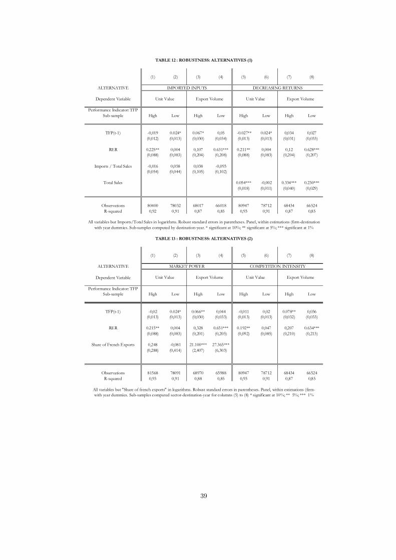
(1) (2) (3) (4) (5) (6) (7) (8)

ALTERNATIVE

Dependent Variable

Performance Indicator: TFPSub-sample High Low High Low High Low High Low

TFP(t-1) -0,019 0.024* 0.067* 0,05 -0.027** 0.024* 0,034 0,027(0,012) (0,013) (0,030) (0,034) (0,013) (0,013) (0,031) (0,033)

RER 0.225** 0,004 0,107 0.631*** 0.211** 0,004 0,12 0.628***(0,088) (0,083) (0,204) (0,208) (0,088) (0,083) (0,204) (0,207)

Imports / Total Sales -0,016 0,058 0,038 -0,093(0,054) (0,044) (0,105) (0,102)

Total Sales 0.054*** -0,002 0.334*** 0.230***(0,018) (0,011) (0,040) (0,029)

Observations 80400 78032 68017 66018 80947 78712 68434 66524R-squared 0,92 0,91 0,87 0,85 0,93 0,91 0,87 0,85

(1) (2) (3) (4) (5) (6) (7) (8)

ALTERNATIVE

Dependent Variable

Performance Indicator: TFPSub-sample High Low High Low High Low High Low

TFP(t-1) -0,02 0.024* 0.066** 0,044 -0,011 0,02 0.078** 0,036(0,013) (0,013) (0,030) (0,033) (0,013) (0,013) (0,032) (0,033)

RER 0.215** 0,004 0,328 0.651*** 0.192** 0,047 0,207 0.634***(0,088) (0,083) (0,201) (0,205) (0,092) (0,085) (0,210) (0,213)

Share of French Exports 0,248 -0,081 21.100*** 27.365***(0,288) (0,414) (2,407) (6,303)

Observations 81568 78091 68970 65988 80947 78712 68434 66524R-squared 0,93 0,91 0,88 0,85 0,93 0,91 0,87 0,85

All variables but "Share of french exports" in logarithms. Robust standard errors in parentheses. Panel, within estimations (firm-with year dummies. Sub-samples computed sector-destination-year for columns (5) to (8) * significant at 10%; ** 5%; *** 1%

Unit Value Export Volume Unit Value Export Volume

TABLE 13 : ROBUSTNESS: ALTERNATIVES (2)

MARKET POWER COMPETITION INTENSITY

TABLE 12 : ROBUSTNESS: ALTERNATIVES (1)

IMPORTED INPUTS DECREASING RETURNS

Unit Value Export Volume Unit Value Export Volume

All variables but Imports/Total Sales in logarithms. Robust standard errors in parentheses. Panel, within estimations (firm-destination with year dummies. Sub-samples computed by destination-year. * significant at 10%; ** significant at 5%; *** significant at 1%

39

Dep. Var. : (1) (2) (3) (4) (5) (6) (7) (8)

Sectoral Export Volume

Sectoral Indicator

Sub-sample High Low High Low High Low High Low

RER 1.147*** 0.709** 1.056*** 0.711*** 0.969** 0.480* 0.850* 0.484*(0.365) (0.277) (0.361) (0.269) (0.431) (0.289) (0.441) (0.281)

RER(t-1) -0.511 0.812*** -0.345 0.728*** -0.304 0.541* 0.000 0.445*(0.342) (0.268) (0.353) (0.262) (0.363) (0.277) (0.394) (0.269)

GDP 1.173** 1.467*** 1.318** 1.491*** 1.701*** 1.370*** 1.825*** 1.445***(0.514) (0.416) (0.521) (0.428) (0.579) (0.454) (0.587) (0.477)

…

Total effect of RER 0.636 1.521*** 0.711 1.440*** 0.665 1.021*** 0.850 0.930***(0.451) (0.365) (0.460) (0.380) (0.491) (0.381) (0.544) (0.395)

Observations 4002 4074 4005 4073 4001 4074 4004 4073R-squared 0.97 0.96 0.96 0.96 0.95 0.97 0.96 0.97

All variables in logarithms. Robust standard errors in parentheses.All estimations include sector-destination

Mean Productivity Median Productivity Mean Productivity Median Productivity

All firms All firms Existing Exporters Existing Exporters

fixed effects and year dummies. * significant at 10%; ** significant at 5%; *** significant at 1%

TABLE 14: EXCHANGE RATE, PRODUCTIVITY AND EXPORT VOLUMES, AGGREGATED

40

Documents

Nicolas Berman, Philippe Martin and Thierry Mayer