NGU REPORT

NGU REPORT 2021.025

ERT and GPR survey at the

Stiksmoen unstable rock slope, Aurland municipality, Vestland county

Geological Survey of Norway P.O.Box 6315 Torgarden NO-7491 TRONDHEIM Tel.: 47 73 90 40 00

REPORT

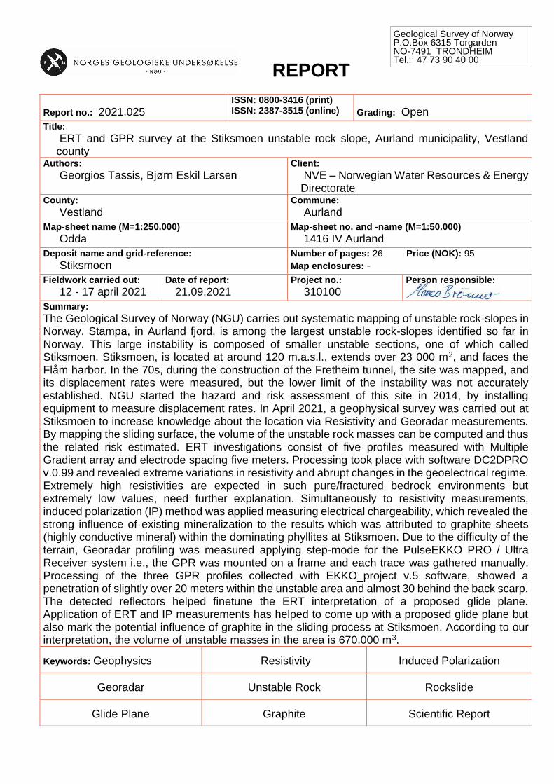
Report no.: 2021.025 ISSN: 0800-3416 (print) ISSN: 2387-3515 (online)

Grading: Open

Title:

ERT and GPR survey at the Stiksmoen unstable rock slope, Aurland municipality, Vestland county

Authors:

Georgios Tassis, Bjørn Eskil Larsen Client:

NVE – Norwegian Water Resources & Energy Directorate

County:

Vestland Commune:

Aurland

Map-sheet name (M=1:250.000)

Odda Map-sheet no. and -name (M=1:50.000)

1416 IV Aurland

Deposit name and grid-reference:

Stiksmoen Number of pages: 26 Price (NOK): 95 Map enclosures: -

Fieldwork carried out:

12 - 17 april 2021 Date of report:

21.09.2021 Project no.:

310100 Person responsible:

Summary:

The Geological Survey of Norway (NGU) carries out systematic mapping of unstable rock-slopes in Norway. Stampa, in Aurland fjord, is among the largest unstable rock-slopes identified so far in Norway. This large instability is composed of smaller unstable sections, one of which called Stiksmoen. Stiksmoen, is located at around 120 m.a.s.l., extends over 23 000 m2, and faces the Flåm harbor. In the 70s, during the construction of the Fretheim tunnel, the site was mapped, and its displacement rates were measured, but the lower limit of the instability was not accurately established. NGU started the hazard and risk assessment of this site in 2014, by installing equipment to measure displacement rates. In April 2021, a geophysical survey was carried out at Stiksmoen to increase knowledge about the location via Resistivity and Georadar measurements. By mapping the sliding surface, the volume of the unstable rock masses can be computed and thus the related risk estimated. ERT investigations consist of five profiles measured with Multiple Gradient array and electrode spacing five meters. Processing took place with software DC2DPRO v.0.99 and revealed extreme variations in resistivity and abrupt changes in the geoelectrical regime. Extremely high resistivities are expected in such pure/fractured bedrock environments but extremely low values, need further explanation. Simultaneously to resistivity measurements, induced polarization (IP) method was applied measuring electrical chargeability, which revealed the strong influence of existing mineralization to the results which was attributed to graphite sheets (highly conductive mineral) within the dominating phyllites at Stiksmoen. Due to the difficulty of the terrain, Georadar profiling was measured applying step-mode for the PulseEKKO PRO / Ultra Receiver system i.e., the GPR was mounted on a frame and each trace was gathered manually. Processing of the three GPR profiles collected with EKKO_project v.5 software, showed a penetration of slightly over 20 meters within the unstable area and almost 30 behind the back scarp. The detected reflectors helped finetune the ERT interpretation of a proposed glide plane. Application of ERT and IP measurements has helped to come up with a proposed glide plane but also mark the potential influence of graphite in the sliding process at Stiksmoen. According to our interpretation, the volume of unstable masses in the area is 670.000 m3.

Keywords: Geophysics

Resistivity

Induced Polarization

Georadar

Unstable Rock

Rockslide

Glide Plane

Graphite

Scientific Report

CONTENTS

1. INTRODUCTION ................................................................................................. 6

2. METHODS ........................................................................................................... 6

2.1 Electrical Resistivity Tomography (ERT) & Induced Polarization (IP) ............ 6

2.2 Ground Penetrating Radar (GPR) ................................................................. 7

3. DATA ACQUISITION / PROCESSING ................................................................ 8

4. ERT INVERSION RESULTS .............................................................................. 12

5. GPR PROCESSING RESULTS ......................................................................... 19

6. INTERPRETATION ............................................................................................ 21

7. CONCLUSIONS ................................................................................................. 25

8. REFERENCES .................................................................................................. 26

FIGURES Figure 2 1: Diagram of measuring procedure that illustrates the setup of the Lund System and the roll-along method for performing measurements (From Dahlin, 1993). ................................................................................................................................... 7 Figure 2 2: From a single GPR signal to a radargram (Benedetto A. & Benedetto F., 2014). ......................................................................................................................... 8 Figure 3.1: Positioning for ERT and GPR profiles conducted at Stiksmoen plotted on Hardangervidda orthophoto (Norge i bilder, 2019) in UTM zone 33N coordinate system. ....................................................................................................................... 9

Figure 3.2: Pictures from the implementation of the ERT survey at Stiksmoen. ...... 10 Figure 3.3: Picture from the implementation of the GPR survey at Stiksmoen. ....... 11 Figure 4.1: Resistivity (top left) and chargeability (bottom left) inversion result for ERT Profile 1 (NW to SE) along with map depicting its positioning at Stiksmoen (top right) and detailed colour scales (bottom right). ................................................................. 14 Figure 4.2: Resistivity (top left) and chargeability (bottom left) inversion result for ERT Profile 2 (NW to SE) along with map depicting its positioning at Stiksmoen (top right) and detailed colour scales (bottom right). ................................................................. 15 Figure 4.3: Resistivity (top left) and chargeability (bottom left) inversion result for ERT Profile 3 (NW to SE) along with map depicting its positioning at Stiksmoen (top right) and detailed colour scales (bottom right). ................................................................. 16 Figure 4.4: Resistivity (top left) and chargeability (bottom left) inversion result for ERT Profile 4 (NW to SE) along with map depicting its positioning at Stiksmoen (top right) and detailed colour scales (bottom right). ................................................................. 17

Figure 4.5: Resistivity (top left) and chargeability (bottom left) inversion result for ERT Profile 5 (SW to NE) along with map depicting its positioning at Stiksmoen (top right) and detailed colour scales (bottom right). ................................................................. 18 Figure 5.1: Radargrams for GPR Profile 1, 2 and 3 along with map depicting their positioning at Stiksmoen. .......................................................................................... 20

Figure 6.1: Superimposed ERT and GPR data for ERT Profile 2 and GPR Profile 3 (top left), ERT Profile 5 and GPR Profile 1 (bottom left) along with positioning (top right). ........................................................................................................................ 22 Figure 6.2: ERT Profiles measured at Stiksmoen and interpreted sliding surface for the unstable slope (black dotted line). ...................................................................... 23 Figure 6.3: Proposed sliding plane for the unstable rock slope at Stiksmoen based on ERT interpretations. All given depth values are relative to terrain surface. .............. 24

TABLES Table I: Coordinates and lengths for ERT profiles in UTM zone 33 North / WGS 84. 9

Table II: Coordinates and lengths for GPR profiles in UTM zone 33 North / WGS 84.9 Table III: Processing modules employed in EKKO_Project v5. ................................ 12

6

1. INTRODUCTION

The concept of applying geophysical methods to obtain information on unstable rock slopes in Norway has attracted increased interest in recent years from both organizations charged with monitoring such areas in the country i.e., the Geological Survey of Norway (NGU) and the Norwegian Water Resources & Energy Directorate (NVE). Implementation of ERT, Refraction Seismic and GPR methods in Åknes (Rønning et al., 2006, Rønning et al., 2007; Tassis & Rønning., 2018,) has led to the establishment of a rich in information geophysical database, whose data processing led to beneficial qualitative and quantitative interpretations on the area. One of the most valuable products geophysics can yield in the context of risk assessment for unstable areas, is a proposed glide plane based on either 3D or 2.5D geophysical interpretations. This means that covering unstable slopes with a series of 2D geophysical profiles, can potentially lead to 3D information on the sliding surface. Among other areas in Norway, NGU carries out systematic mapping of Stampa in Aurland fjord, which is among the largest unstable rock-slopes identified so far in the country. This large instability is composed of smaller unstable sections, one of which is called Stiksmoen and is the focus of this report. Stiksmoen, is located at around 120 m.a.s.l., extends over 23 000 m2, and faces the Flåm harbor. In the 70s, during the construction of the Fretheim tunnel, the site was mapped, and its displacement rates were measured, but the lower limit of the instability was not accurately established. NGU started the hazard and risk assessment of this site in 2014, by installing equipment to measure displacement rates. In April 2021, a geophysical survey was carried out at Stiksmoen together with NVE to increase knowledge about this part of the instability via mainly Resistivity and supplementary Georadar measurements. The goal of the survey is to map the sliding surface in order to compute the volume of the unstable rock masses and thus estimate the related risk.

2. METHODS

The main geophysical method employed in this survey is Electrical Resistivity Tomography (ERT), which is known to accurately map geoelectrical contrasts in bedrock based on fracturing or lack thereof, water content or lack thereof, mineralization etc. In all ERT surveys NGU conducts, chargeability is also measured alongside resistivity with the use of Induced Polarization (IP) method. Lastly, Ground Penetrating Radar (GPR or Georadar) was also employed even though the method’s achieved penetration is not guaranteed as in ERT and is controlled by the dielectric regime in the ground.

2.1 Electrical Resistivity Tomography (ERT) & Induced Polarization (IP)

The 2D ERT and IP methods are carried out by injecting current into the ground with the use of two electrodes and by measuring the voltage between two separate ones. Based on measured resistance (measured voltage / injected current) and a geometrical factor dependent on the electrode positions, the apparent resistivity and IP effect can then be calculated. The 2D ERT/IP measurements were performed after

7

the Lund cable system (Dahlin, 1993) while ABEM Terrameter LS (ABEM, 2012) is the NGU in-house system for acquiring data. As seen in Figure 2.1, four multi-electrode cables are used to measure in the Multiple Gradient electrode configuration (Dahlin & Zhou, 2006). Once the electrodes are connected to the ground and the cables to the instrument, an automated measuring procedure starts, by transmitting current through one electrode pair and measuring electric potential at another (up to four electrode pairs simultaneously). Resistivity is measured when the injected electric current is on, while IP-effect is measured shortly after cutting it. The electrode separation controls depth coverage and for 2, 5 and 10 m electrode distance, the penetration depth is ca. 20, 60 m and 120 m respectively, depending on the resistivity in the ground. Generally, resolution decreases with depth and deeper parts of the resistivity sections are, by experience, of low reliability.

Figure 2 1: Diagram of measuring procedure that illustrates the setup of the Lund

System and the roll-along method for performing measurements (From Dahlin, 1993).

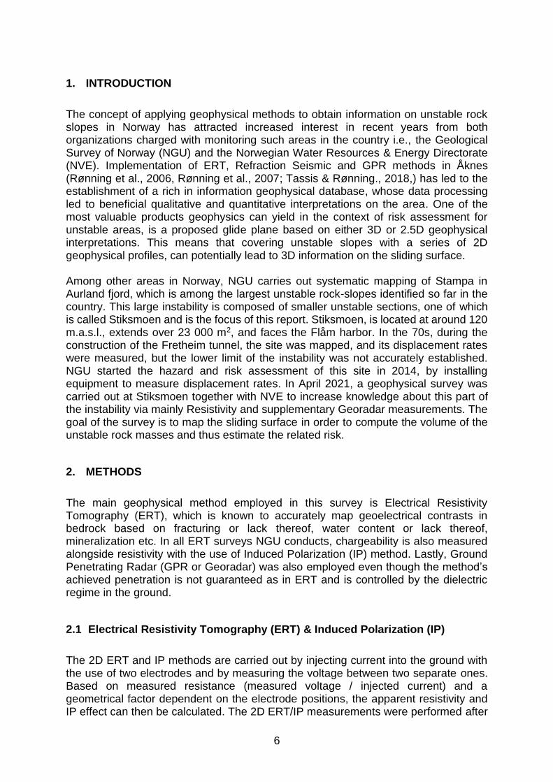
2.2 Ground Penetrating Radar (GPR)

Ground Penetrating Radar (GPR), or Georadar as is also commonly called, is an electromagnetic geophysical technique which can be used to investigate stratification in the underground. It uses electromagnetic fields to probe lossy dielectric materials to detect structures and changes in material properties within the materials (Davis & Annan,1989). With GPR, the electromagnetic fields propagate as essentially nondispersive waves. The signal emitted travels through the material, is scattered and/or reflected by changes in impedance, giving rise to events which appear similar to the emitted signal (Butler, 2005). These reflected signals are registered at the surface and utilized to reconstruct interfaces in the ground. This is achieved by the compilation images where 1D electromagnetic “soundings” are positioned consecutively to create a uniform 2D image (radargram – figure 2.2). In lossy dielectric materials, electromagnetic fields can only penetrate to a limited depth before being absorbed. Hence, exploration depth is always a variable. However, the frequency range where GPR functions is between 1 and 1000 MHz, and the choice of frequency

8

also controls the projected depth of an investigation. In lower frequencies, the pulses are easily dispersed while at higher frequencies the signal absorption becomes too strong and the penetration depth extremely limited. GPR studies are therefore planned with a frequency choice that compromises penetration depth (lower frequencies) with desired signal resolution (higher frequencies) in relation to the survey goals.

Figure 2 2: From a single GPR signal to a radargram (Benedetto A. & Benedetto F.,

2014).

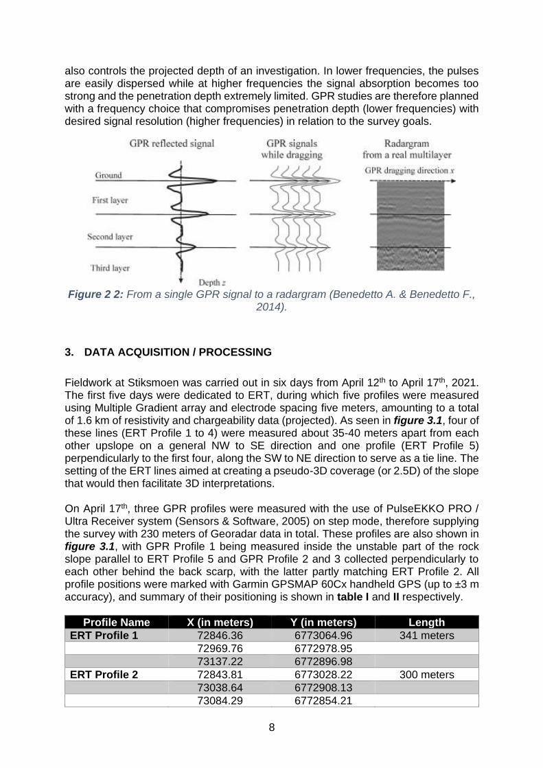
3. DATA ACQUISITION / PROCESSING

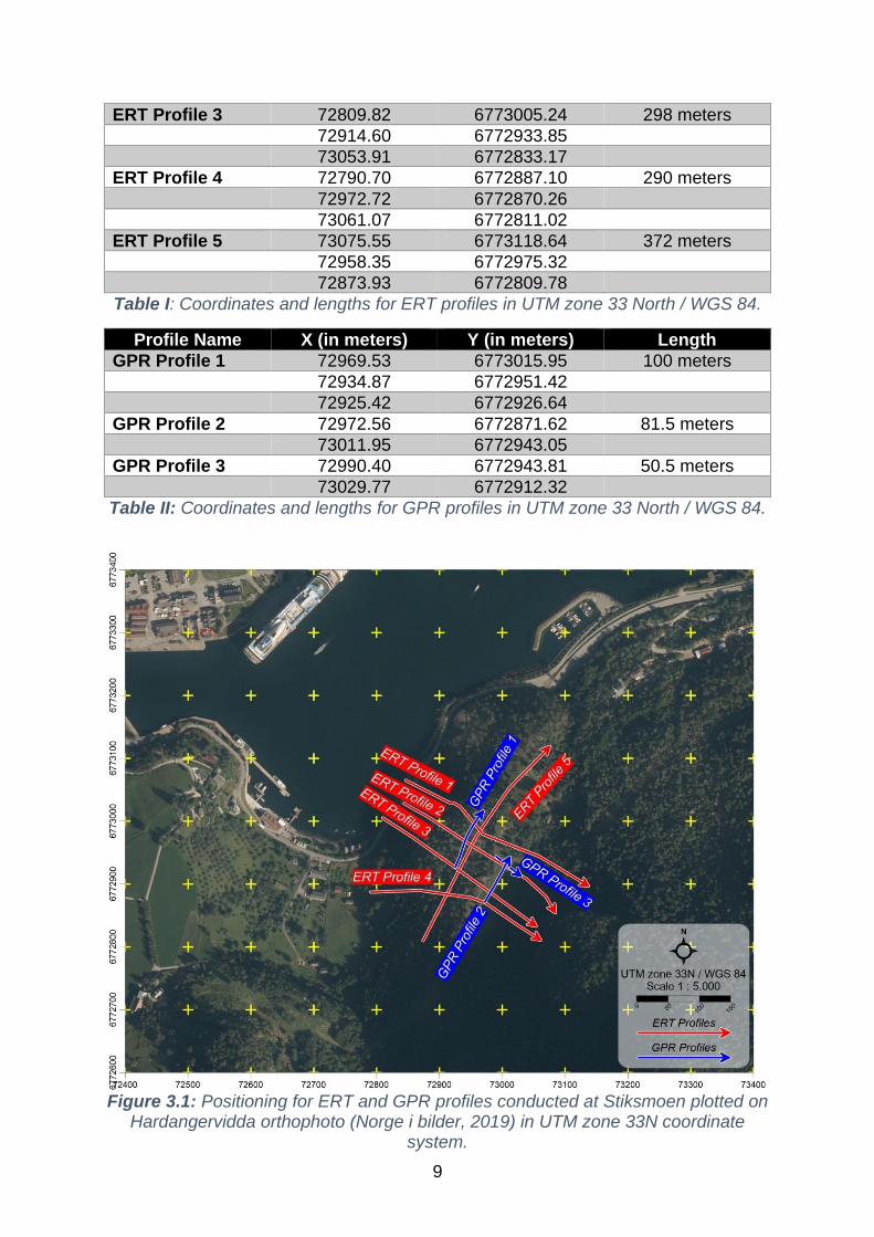
Fieldwork at Stiksmoen was carried out in six days from April 12th to April 17th, 2021. The first five days were dedicated to ERT, during which five profiles were measured using Multiple Gradient array and electrode spacing five meters, amounting to a total of 1.6 km of resistivity and chargeability data (projected). As seen in figure 3.1, four of these lines (ERT Profile 1 to 4) were measured about 35-40 meters apart from each other upslope on a general NW to SE direction and one profile (ERT Profile 5) perpendicularly to the first four, along the SW to NE direction to serve as a tie line. The setting of the ERT lines aimed at creating a pseudo-3D coverage (or 2.5D) of the slope that would then facilitate 3D interpretations. On April 17th, three GPR profiles were measured with the use of PulseEKKO PRO / Ultra Receiver system (Sensors & Software, 2005) on step mode, therefore supplying the survey with 230 meters of Georadar data in total. These profiles are also shown in figure 3.1, with GPR Profile 1 being measured inside the unstable part of the rock slope parallel to ERT Profile 5 and GPR Profile 2 and 3 collected perpendicularly to each other behind the back scarp, with the latter partly matching ERT Profile 2. All profile positions were marked with Garmin GPSMAP 60Cx handheld GPS (up to ±3 m accuracy), and summary of their positioning is shown in table I and II respectively.

Profile Name X (in meters) Y (in meters) Length

ERT Profile 1 72846.36 6773064.96 341 meters

72969.76 6772978.95

73137.22 6772896.98


73038.64 6772908.13

73084.29 6772854.21

9


72914.60 6772933.85

73053.91 6772833.17


72972.72 6772870.26

73061.07 6772811.02


72958.35 6772975.32

72873.93 6772809.78

Table I: Coordinates and lengths for ERT profiles in UTM zone 33 North / WGS 84.

Profile Name X (in meters) Y (in meters) Length

GPR Profile 1 72969.53 6773015.95 100 meters

72934.87 6772951.42

72925.42 6772926.64

GPR Profile 2 72972.56 6772871.62 81.5 meters

73011.95 6772943.05

GPR Profile 3 72990.40 6772943.81 50.5 meters

73029.77 6772912.32

Table II: Coordinates and lengths for GPR profiles in UTM zone 33 North / WGS 84.

Figure 3.1: Positioning for ERT and GPR profiles conducted at Stiksmoen plotted on

Hardangervidda orthophoto (Norge i bilder, 2019) in UTM zone 33N coordinate system.

10

All measurements were conducted under good weather conditions, starting from relatively cold and gradually improving to warmer. Due to the steep inclination of the terrain, a number of electrodes had to be positioned with the help of climbing equipment and valuable help from NVE employees (figure 3.2). Moreover, another group of electrodes had to be excluded from each profile (maximally 5 out of 81 for ERT Profiles 1 to 3), due to the presence of bare rock and the lack of soil and/or organic material to establish connection with the ground. This resulted in gaps inside the trapezoidal coverage of the ERT data, but without any severe effect on the desired resolution. Lastly, all profiles extend over very steep terrain and therefore appear shorter in projected length shown in table I even though measured in full outlays of 400 meters or slightly less.

Figure 3.2: Pictures from the implementation of the ERT survey at Stiksmoen.

Concerning the GPR survey, the steepness and of the terrain and hazard related to deep cracks on the ground especially within the unstable part of the slope, made the choice of step mode measurements necessary. To maximize penetration at Stiksmoen, the frequency selected was the lowest available i.e., 50 MHz which requires transmitter and receiver antennas to be positioned at two meters apart. As

11

seen in figure 3.3, this specification increases the bulk of the mounting frame, thus making carrying and manoeuvring in such terrain even more difficult, especially for flat antennas laying on steeply inclined bare rock. Despite that, since the system utilized was PulseEKKO PRO with the Ultra Receiver unit, it was possible to use a high number of stacks, namely 8192 on each trace assembled and thus indirectly increase the penetration depth and data quality. Traces were registered manually every 0.5 m (two seconds per measurement) along a measuring tape laid to the ground for reference as also seen in figure 3.3.

Figure 3.3: Picture from the implementation of the GPR survey at Stiksmoen.

ERT processing took place with software DC2DPRO v.0.99 (Kim, 2009) for resistivity and RES2DINV v.4.8.18 (Loke, 2018) for chargeability. Since the survey is focused on interpreting the instability’s sliding surface, inversion for resistivity was ran using standard constraint (L2-norm) for both model and data. This choice was made to facilitate inversion in better visualizing horizontal layering. Minor filtering of data took place by eliminating faulty measurements after each inversion to ensure RMS error would be within reasonable levels. Even the resulting error percentages were around 10%, inversion revealed extreme variations in resistivity and abrupt changes in the geoelectrical regime. Extremely high resistivities are expected in bedrock (phyllites) but extremely low values, need further explanation. Inversion of the IP data also showed big variations in chargeability, which can be attributed to existing mineralization. Error in these inversion results is quite big and is induced by sharp contrasts in chargeability. Such a strong influence is due to graphite within the dominating phyllites that has been identified at Stiksmoen, a highly conductive mineral that can create strong IP effect even in thin sheets intertwined in bedrock. In this context, chargeability inversion results can be used to identify areas of extremely low resistivity where mineralization is the cause and not bad bedrock quality or water content. However, it must be noted that inversion results for resistivity and chargeability might be slightly different depending on how each inversion software

12

incorporates steep topography in the results. DC2DPRO inverts resistivity with topography while RES2DINV without, adjusting the results to topography afterwards. All collected GPR data were processed with software package EKKO_Project v.5. Quality wise, the data collected inside the unstable area are better than the ones measured behind the back scarp. GPR Profile 2 and 3 are plagued by ambient noise which is mainly coming from power cables running very close to the survey area but also huge boulders that reflect air waves transmitted by the Georadar. Table III presents a summarized description of the modules used to process the GPR data. It should be noted that the velocity employed for both depth conversion and migration is the default one (0.1 m/ns). Migration was necessary regardless of the lack of CMP (Common Mid-Point) measurement, to collapse many hyperbolas in the data coming from true ground targets. Generally, a very high number of stacks like the one used in this survey, increases reflectivity from possible point targets in the ground. The downside is that all air wave hyperbolas have acquired the form of the letter U, thus creating artefacts in the results. This was of course considered during interpretation.

Processing module Value / Description

Bandpass Filter Fc1 20 % / Fp1 60 % / Fp2 140 % / Fc2 180 %

Depth Conversion Velocity 0.1 m/ns

Dewow Window Width (Pulse Widths): 1.33

Background Subtraction Filter Width: 20 m (rectangular)

SEC2 Gain Attenuation 0.65 - 1.35 dB/m, Start Gain 0.4 – 1.25, Maximum Gain 250 - 2000

Table III: Processing modules employed in EKKO_Project v5.

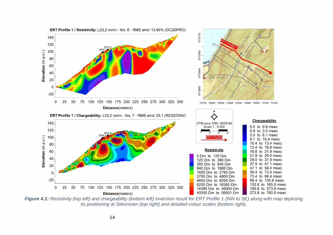
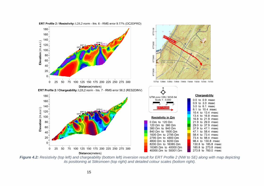
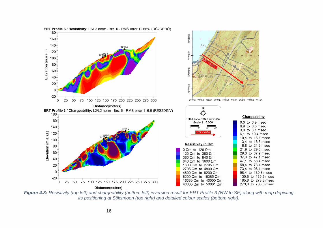
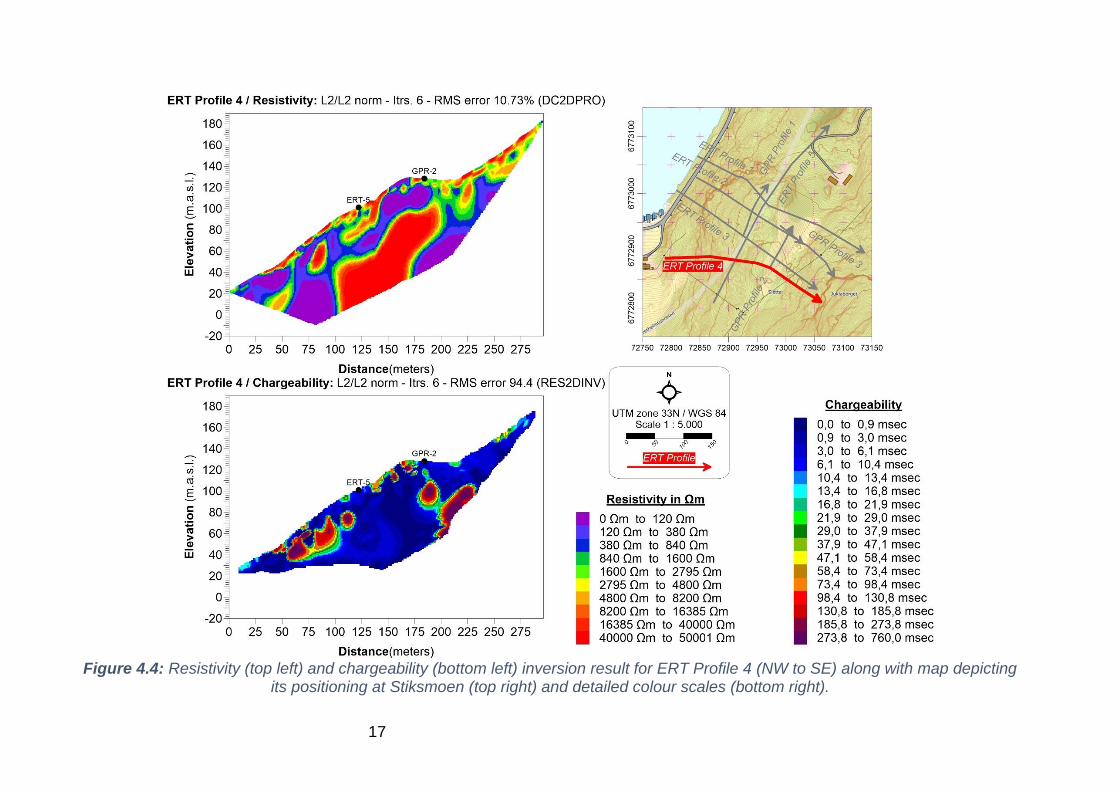
4. ERT INVERSION RESULTS

ERT resistivity and chargeability results are presented using the colour scales typically employed by the inversion software i.e., standard rainbow for DC2DPRO and spectral for RES2DINV. Both colour scales are identical for all results and is calculated to represent the geoelectrical regime at Stiksmoen in its entirety. It must be noted that the trapezoid depth coverage for each profile is similar but not identical for resistivity and chargeability, due to the use of different inversion software. However, the results are directly comparable. Elevation is extracted by LiDAR point cloud for Sogndal – Aurland – Lærdal (Kartverket Bergen, 2014). Results for ERT Profile 1 are shown in figure 4.1 and depict high contrasts both on resistivity and chargeability. The profile on the top left side of the figure which displays resistivity, can be divided into two geoelectrical regimes based on the back scarp at 175 meters, even though a quite prominent vertical low resistivity anomaly is found at about 200 meters distance. This anomaly is characterized by resistivities less than 120 Ωm (purple colour) which is extremely low for any phyllite, and therefore one can assume that graphite sheets play a big role in this. To the right of this anomaly, resistivities are consistently much higher than the left which indicates bedrock of better quality. To the left of the back scarp and inside the unstable area, extremely high and low resistivity packages become interchanged both laterally and vertically, creating a challenging image for interpretation. Generally, areas of very high resistivity are probably due to cracks in bedrock that stop the propagation of the electrical current

13

and therefore appear as high resistors in the results. Looking at the chargeability inversion result left of the backscarp in the bottom left of figure 4.1, blobs of high chargeability values (red - brown colors) do not necessarily match low resistivities, indicating that graphite sheets affect ERT measurements in a complex way that is problematic to understand, especially concerning the extremely low resistivity flat cluster near the fjord, to the far left of ERT Profile 1. Figure 4.2 shows the respective results for ERT Profile 2 and presents similar conditions to ERT Profile 1, but also a bit clearer in terms of resistivity and chargeability distribution. Again, the back scarp is represented misplaced by a vertical low resistivity anomaly, left of which where the unstable slope is, resistivity interchanges between very low and very high value packages. However, what is fundamentally different here is that there appears to be a sub horizontal stratification in resistivity, outlined by continuous clusters of low values sitting on top of high resistivity bodies. This transition could potentially mark the sliding surface but also indicate that unstable rock gliding at Stiksmoen is facilitated or controlled by graphite. Another difference in this profile is that areas of high chargeability match areas of low resistivity much better, even though with some offset due to how each software incorporates topography in inversion. ERT Profile 3 depicted in figure 4.3 continues with the established pattern shown in ERT Profile 2 i.e., a top layer of low resistivities overlaying what could appear as resistive bedrock and a back scarp that is represented misplaced again by a prominent low resistivity anomaly. Chargeability is in good agreement with resistivity for this profile too, except for an area at around 150 meters distance where a high chargeability anomaly is not matched by low resistivity, but instead the highly resistive bedrock seems to weakly split in two smaller parts. Another interesting feature seen in ERT Profile 3, as the scanning of the slope with NW to SE profiles moves southwards, is that contrasts between high and low values in resistivity and chargeability are becoming more abrupt. This means that the shift from very high to very low resistivities and chargeabilities is not gradual but happens over shorter distance, thus creating more sharp boundaries (from purple to red for example). This could indicate a stronger overall presence of graphite on that part of the slope. Figure 4.4 presents ERT Profile 4 which appears to be quite like ERT Profile 3 i.e., the calculated contrasts in resistivity and chargeability are sharp with the possible glide plane lying inside the low resistivity zone overlaying the highly resistive bedrock. However, this profile presents the highest content in low resistivity and the lowest in high chargeability out of all the profiles seen so far. High chargeability is now found nearer the fjord and at the back scarp, but low resistivities are still dominant in the entire depth coverage of the ERT Profile 4. This could potentially indicate more concentrated and purer graphite in that part of the slope, that is still greatly affecting measured resistivity. However, the error in chargeability inversion is quite high, therefore results here are not entirely trustworthy. ERT Profile 5 shown in figure 4.5 summarizes the changes in the geoelectrical regime seen in the previous profiles by being perpendicular to them and following a southwest to northeast direction, well inside the unstable area. Both resistivity and chargeability in ERT Profile 5 register a low resistivity top layer which is much more pronounced in the south due to higher contrasts and becoming less evident in the north of the unstable slope. The high error in chargeability inversion does not allow much trust to be put on these data, but the general outlook is quite similar to what has been extracted so far.

14

Figure 4.1: Resistivity (top left) and chargeability (bottom left) inversion result for ERT Profile 1 (NW to SE) along with map depicting

its positioning at Stiksmoen (top right) and detailed colour scales (bottom right).

15



16



17



18

Figure 4.5: Resistivity (top left) and chargeability (bottom left) inversion result for ERT Profile 5 (SW to NE) along with map depicting


19

5. GPR PROCESSING RESULTS

For presenting the GPR processing results from the profiles gathered at Stiksmoen, a similar plan is used as in ERT, but this time with all results summarized in figure 5.1 due to their limited extent compared to ERT. The colour scale used is the standard greyscale for GPR, where strong reflectors are shown in alternating black and white bands and weaker ones in hues of grey respective to their magnitude. Again, positioning for all profiles is shown with the use of a smaller map incorporated in the figure with elevation along the profiles extracted from LiDAR dataset for Sogndal – Aurland – Lærdal (2014). GPR Profile 1 is the most noise-free profile out of all the measured profiles at Stiksmoen since it has been measured inside the unstable rock slope and away from power cables. Depth penetration here is roughly 20 meters and mainly detects horizontal reflectors. Signal strength is not continuously strong, with certain areas revealing more changes in impedance than others, like from 0 to 20 and 40 to 60 meters distance. What is most interesting though, is the fact that penetration is generally homogeneous throughout GPR Profile 1, and the signal collectively deteriorates to background noise at about 85 m.a.s.l. In other words, this could be an indication for the sliding surface, where fractured bedrock, regardless of being infilled with soil or not, is giving place to massive or unfractured stone that presents the electromagnetic signal no possibilities for reflection. GPR Profile 2 and 3 on the other hand are measured perpendicular to each other and are plagued by ambient noise. This ambient noise comes into the presented radargrams in figure 5.1 in the form of many inverted hyperbolas or more plainly U-shaped reflectors. This effect is inherited into the results by an otherwise necessary processing action which is migration. Utilizing thousands of stacks to strengthen the Georadar signal like we did at Stiksmoen, makes reflections from smaller point targets into the ground become strengthened and therefore appear in the raw data as real ground hyperbolas or in other words, true underground signal. Collapsing these hyperbolas to points requires migration, but this action also affects all existing hyperbolas found in a radargram. As mentioned before, airwaves from targets above the ground at Stiksmoen (huge boulders, power cables, etc) created undesired hyperbolas that are much wider since the electromagnetic signal travels above ground at the speed of light. When applying migration, these hyperbolas are also affected and become inverted because the velocity used for migration is much smaller than that of the speed of light. As can easily be seen, both GPR Profiles performed close to the power lines shown on the map by the continuous black line, contain a higher noise level. Ignoring the ambient noise in GPR Profile 2 and 3, several horizontal reflectors can be identified throughout the length of both lines, in addition to some deeper ones inclined towards the north. Signal penetration acquires its maximum value of almost 30 meters at the end of both profiles i.e., the northern part of the area they cover. This is indicative of sediment infills on the plateau behind the back scarp where a small farming field is found.

20

Figure 5.1: Radargrams for GPR Profile 1, 2 and 3 along with map depicting their positioning at Stiksmoen.

21

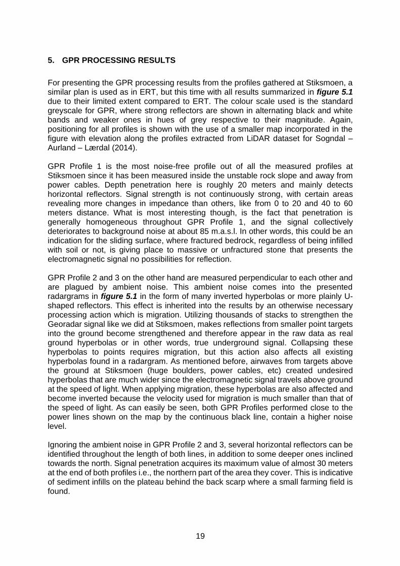
6. INTERPRETATION

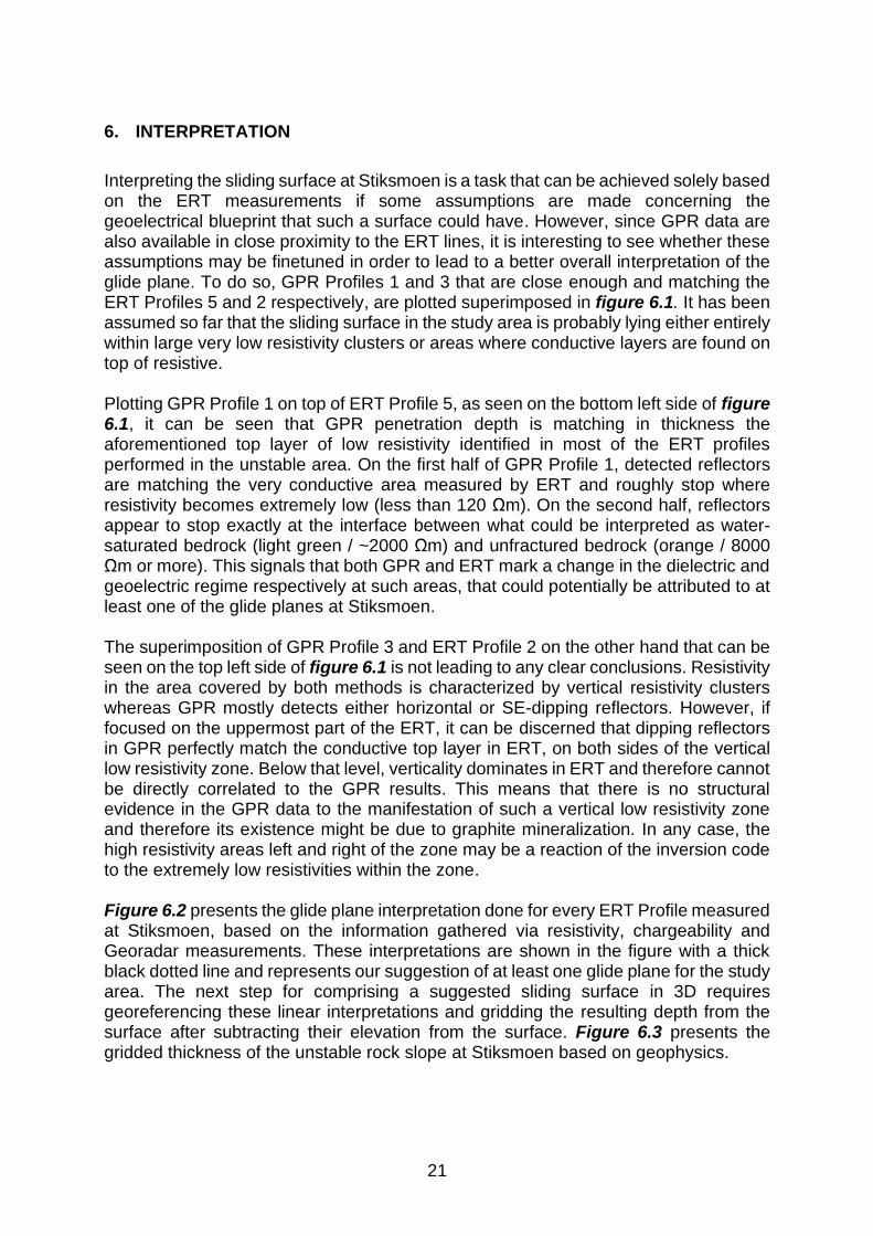
Interpreting the sliding surface at Stiksmoen is a task that can be achieved solely based on the ERT measurements if some assumptions are made concerning the geoelectrical blueprint that such a surface could have. However, since GPR data are also available in close proximity to the ERT lines, it is interesting to see whether these assumptions may be finetuned in order to lead to a better overall interpretation of the glide plane. To do so, GPR Profiles 1 and 3 that are close enough and matching the ERT Profiles 5 and 2 respectively, are plotted superimposed in figure 6.1. It has been assumed so far that the sliding surface in the study area is probably lying either entirely within large very low resistivity clusters or areas where conductive layers are found on top of resistive. Plotting GPR Profile 1 on top of ERT Profile 5, as seen on the bottom left side of figure 6.1, it can be seen that GPR penetration depth is matching in thickness the aforementioned top layer of low resistivity identified in most of the ERT profiles performed in the unstable area. On the first half of GPR Profile 1, detected reflectors are matching the very conductive area measured by ERT and roughly stop where resistivity becomes extremely low (less than 120 Ωm). On the second half, reflectors appear to stop exactly at the interface between what could be interpreted as water-saturated bedrock (light green / ~2000 Ωm) and unfractured bedrock (orange / 8000 Ωm or more). This signals that both GPR and ERT mark a change in the dielectric and geoelectric regime respectively at such areas, that could potentially be attributed to at least one of the glide planes at Stiksmoen. The superimposition of GPR Profile 3 and ERT Profile 2 on the other hand that can be seen on the top left side of figure 6.1 is not leading to any clear conclusions. Resistivity in the area covered by both methods is characterized by vertical resistivity clusters whereas GPR mostly detects either horizontal or SE-dipping reflectors. However, if focused on the uppermost part of the ERT, it can be discerned that dipping reflectors in GPR perfectly match the conductive top layer in ERT, on both sides of the vertical low resistivity zone. Below that level, verticality dominates in ERT and therefore cannot be directly correlated to the GPR results. This means that there is no structural evidence in the GPR data to the manifestation of such a vertical low resistivity zone and therefore its existence might be due to graphite mineralization. In any case, the high resistivity areas left and right of the zone may be a reaction of the inversion code to the extremely low resistivities within the zone. Figure 6.2 presents the glide plane interpretation done for every ERT Profile measured at Stiksmoen, based on the information gathered via resistivity, chargeability and Georadar measurements. These interpretations are shown in the figure with a thick black dotted line and represents our suggestion of at least one glide plane for the study area. The next step for comprising a suggested sliding surface in 3D requires georeferencing these linear interpretations and gridding the resulting depth from the surface after subtracting their elevation from the surface. Figure 6.3 presents the gridded thickness of the unstable rock slope at Stiksmoen based on geophysics.

22

Figure 6.1: Superimposed ERT and GPR data for ERT Profile 2 and GPR Profile 3 (top left), ERT Profile 5 and GPR Profile 1 (bottom

left) along with positioning (top right).

23

Figure 6.2: ERT Profiles measured at Stiksmoen and interpreted sliding surface for the unstable slope (black dotted line).

24

Figure 6.3: Proposed sliding plane for the unstable rock slope at Stiksmoen based on ERT interpretations. All given depth values are relative to terrain surface.

25

The proposed sliding surface shown in figure 6.3 displays the thickness distribution of unstable rock along the slope at Stiksmoen. According to this interpretation, unstable masses can be as thick as 40 meters below surface, but its mean value is 25 meters. Besides a few variations, the most unstable part of the slope is delineated by the hanging rock topography and framed by the steepest changes in elevation as seen with the brown lines in the figure. The calculated unstable rock volume between proposed glide plane and surface for this scenario is 670.000 cubic meters. However, additional information such as drilling in the area could further help to determine a more accurate calculation of the rock volume hazardous to slide into Aurland fjord during a possible rockslide.

7. CONCLUSIONS

Applying geophysics in difficult terrain has shown that surveys such as the one performed at Stiksmoen require more working hands and time than usual in order to be performed both effectively and safely. The fact that weather conditions during measurements were dry, has facilitated measurements in terms of crew safety and overall performance. Climbing skills also proved to be an integral part of the success of carrying out the survey, while the inability to connect electrodes on bare rock has not affected the resolution of the ERT investigation. GPR on the other hand was limited to relatively flat areas due to the usage of a mounting frame that could make measuring not only impossible on the roughest spots but also dangerous. The ERT and GPR surveys at Stiksmoen have proven to be a useful tool in describing the structural regime in the area and proposing a glide plane based on the results obtained by geophysics. Resistivity and chargeability measurements have detected the existence of a high conductor in the ground that greatly affects all geoelectrical measurements. Observances of graphite in the study area indicate that sheets of this highly conductive mineral are found in the phyllites and thus cause both high IP effect and extremely low resistivities measured. However, the existence of such a strong conductor in a highly resistive bedrock environment creates very high contrasts in the measured resistivity and destabilizes the inversion process. On the northern part of the slope, ERT measurements revealed more gradual distribution of resistivity whereas in the south, changes of many thousands of Ωm happen over a few meters. Regardless, by also using the penetration depth of GPR profiles measured in the area and comparing them against the ERT results, it has been concluded that the sliding surface at Stiksmoen should be sought at areas of low resistivity, especially in the case where they lay on top of resistive blocks. This also indicates that graphite is very probable to play a big role in the sliding mechanics of the unstable slope and should be investigated in more detail. By digitizing a proposed glide plane on all ERT profiles, georeferencing it and lastly gridding the results, we were able to calculate the thickness of the unstable masses according to geophysics and subsequently calculate their projected volume. This was found to be equal to 670.000 cubic meters of rock that could potentially feed a rockslide in the area. Lacking further information such as drilling, we are not able to discern the accuracy of this calculation, but resistivity has proven to be quite effective in mapping such areas in the past, therefore results based on the method are quite trustworthy.

26

8. REFERENCES

ABEM, 2012: ABEM Terrameter LS. Instruction Manual. ABEM Product Number 33

3000 95, ABEM 20121025, based on release 1.11. ABEM, Sweden. Butler, D.K. (edited), 2005: Near Surface Geophysics (Investigations in Geophysics

No. 13). Society of Exploration Geophysicists, ISBN: 1-56080-130-1 (Volume - 756 pp.).

Davis, J.L., and Annan, A.P., 1986: Borehole radar sounding in CR-6, CR-7 and CR-8

at Chalk River, Ontario: Technical Record TR-401, Atomic Energy of Canada Ltd. Dahlin, T., 1993: On the Automation of 2D Resistivity Surveying for Engineering and

Environmental Applications. Dr. Thesis, Department of Engineering Geology, Lund Institute of Technology, Lund University. ISBN 91-628-1032-4.

Dahlin T. & Zhou B., 2006: Multiple-gradient array measurements for multi-channel 2D

resistivity imaging. Near Surface Geophysics, 4. 113-123. Kartverket Bergen, 2014: Sogndal – Aurland – Lærdal LiDAR point cloud, Project

number LACHSF33, Blom Geomatics, www.hoydedata.no. Kim J.H., 2009. DC2DPro-2D Interpretation System of DC Resistivity Tomography.

User’s Manual and Theory, KIGAM, S. Korea. Loke, M.H., 2017: RES2DINVx64 ver. 4.07. Rapid 2-D Resistivity & IP inversion using

the least-squares method. Geotomo Software, August 2017. - www.geotomosoft.com

Norge i Bilder, 2019: Hardangervidda Orthophoto, www.norgeibilder.no. Rønning, J.S., Dalsegg, E., Elvebakk, H., Ganerød, G. & Tønnesen, J.F., 2006:

Geofysiske målinger Åknes og Tafjord, Stranda og Nordal kommuner, Møre og Romsdal. NGU Rapport 2006.02.

Rønning, J.S., Dalsegg, E., Heincke, B.H. & Tønnesen, J.F., 2007: Geofysiske

målinger på bakken ved Åknes og ved Hegguraksla, Stranda og Nordal kommuner, Møre og Romsdal. NGU Rapport 2007.026.

Sensors & Software, 2005: PulseEKKO PRO – Product Manual., 2005-00040-09,

Sensors & Software Inc., Mississauga, Ontario - Canada. Tassis, G. & Rønning, J.S., 2018: Reprocessing of ERT data from Åknes, Stranda

Municipality, Møre & Romsdal County. NGU Report 2018.002.

http://www.hoydedata.no/

http://www.norgeibilder.no/

Documents

NGU REPORT