NGST Monograph No. 6 Performance Analysis Using Integrated Modeling · 2015-07-02 · NGST Monograph No. 6 Performance Analysis Using Integrated Modeling By Gary Mosier, Keith Parrish,

NGST Monograph No. 6 Performance Analysis

Using Integrated Modeling

By

Gary Mosier, Keith Parrish, Michael Femiano

NASA Goddard Space Flight Center

David Redding, Andrew Kissil, Miltiadis Papalexandris Jet Propulsion Laboratory

Larry Craig, Tim Page, Richard Shunk

NASA Marshall Space Flight Center

August 2000

Next Generation Space Telescope Project Study Office

Goddard Space Flight Center

Executive Summary

The so-called “Yardstick” design concept for the Next Generation Space Telescope presents unique challenges for systems-level analysis. Simulations that integrate controls, optics, thermal and structural models are required to evaluate baseline performance, study design sensitivities, and perform design optimization. An integrated modeling approach was chosen, and simulations were built using a combination of commercial off-the-shelf and in-house developed codes. The resulting capability provides a foundation for linear and non-linear analysis, using both the time and frequency-domain methods. It readily allows various combinations of design parameters and environmental loads to be evaluated directly in terms of key science-related metrics, specifically centroid error and RMS wavefront error. This document first describes the development of the component, or discipline, models of the Yardstick. It then proceeds to show how the component models are linked to perform two of the most critical baseline performance analyses. These are the static (thermal/structural) stability and dynamic (jitter) stability analyses. The results of the static analysis indicate that the changes in shape due to ground-to-orbit bulk cool-down of the telescope structure are within the expected capture range of the baseline wavefront sensor. This means we will be able to align and phase the segmented primary mirror. However, the results for a quasi-static analysis of a thermal transient event show that the telescope is not passively stable. Either structural re-design or active wavefront control is required during and after a slew maneuver. Use of active thermal control with heaters was demonstrated to be feasible using the models. Finally, the results of the dynamic analysis indicate that disturbances from the reaction wheels coupled with the lightly-damped and highly-flexible structure present significant challenges to the baseline line-of-sight control architecture. Vibration isolation will be required to meet jitter error requirements.

1. Overview of Integrated Modeling for NGST

The Next Generation Space Telescope will provide at least ten times the collecting area of the Hubble Space Telescope in a package that fits into the shroud of an expendable launch vehicle. Several concepts for NGST have been developed and studied. The performance analysis of the so-called NASA “Yardstick” concept [1], using integrated, or multi-disciplinary, modeling techniques, is presented here. Several key features of the Yardstick concept are illustrated in Figure 1-1. The science requirements for NGST are a challenge to the engineering design of this large, lightweight, flexible structure. Specifically, the stability of the images during science operations may be difficult to maintain in the presence of dynamic (jitter) and quasi-static (thermal drift) effects that both alter the co-alignment of the optics and produce changes to the figure of the primary mirror. However, the results of the analysis indicate that by means of careful design coupled with adequate testing to verify material behavior and component performance, the science

requirements can be achieved.

Figure 1-1 NASA “Yardstick” concept for NGST The integrated modeling process for the Yardstick performance analysis was carried out using an evolving suite of multi-disciplinary computer aided design, analysis, and simulation tools. These tools are bound together using the Matlab environment in a manner depicted in Figure 1-2. Matlab provides the core capability to easily manipulate large matrices and to perform numerical analysis in both time and frequency domain. Central to the integrated models are the multidisciplinary capabilities of IMOS [2], a set of Matlab functions developed at the Jet Propulsion Laboratory (JPL) that are used for structural and thermal models. IMOS is highly

Space support module(attitude control,communications, power,data handling) is onwarm side

“Open” telescope (noexternal baffling)allows passivecooling to 50K

Deployable secondarymirror

Berylliumprimary mirror

ScienceInstruments

Large (200m2) deployablesunshield protects from sun,earth and moon

Isolation truss

integrated with another JPL-developed code, MACOS [3], that provides optical ray-trace and diffraction capabilities. Finally, IMOS is also integrated with “legacy” discipline-specific tools such as NASTRAN (structures) and SINDA (thermal).

Figure 1-2 NGST integrated modeling environment These tools and associated integrated modeling techniques, largely employing linear systems theory, were applied to assess the performance of this NGST concept during science operations. The end-to-end models can be, and were, used for a variety of analyses. This report, however, presents results only from the two principal studies performed during the evolution of the Yardstick concept. Prior to presenting the results, the component models (structures, optics, thermal, control, dynamic disturbance – see Figure 1-2) are provided, along with details as to how they were integrated for the end-to-end analyses. The first study is an analysis of the sensitivity of the structure to thermal variations that occur after an attitude maneuver. The initial conditions for the analysis are that the observatory starts with the sun normal to the sunshield and with the optics assumed optimally aligned and phased through use of the wavefront control system. In this attitude, the Optical Telescope Assembly (OTA) bulk temperature is at the maximum. The observatory then executes a pitch-axis slew of 25 degrees, the maximum allowable pitch angle to the sun, which takes the OTA bulk temperature to the minimum. The resulting delta-T, on the order of 1 degree K, produces structural deformations in the OTA and degrade the image quality below the science requirements. The wavefront control system can easily compensate for this, but at a cost to observing efficiency due to the time required to take images, estimate the wavefront error, and reposition the segment and deformable mirror actuators. A design alternative is explored using the integrated models that provides for continuous wavefront stability via active thermal control of the OTA.

DESIGNPARAMETERS

MODELINGTOOLS

SYSTEM MODEL

THERMALDISTURBANCES

MECHANICALDISTURBANCES

ControlDesign

StructureDesign

OpticsDesign

MATLABIMOS FEMNASTRAN

STRUCTURE

CONTROLS

OPTICS

SCIENCEMETRICS

TRASYS /SINDA

SYSTEM PERFORMANCE

MATLAB

ENVIRONMENT

OPTICALERRORS

∫

MACOS

The second study is an analysis of the effect of reaction wheel dynamic disturbances upon image stability. The observatory pointing control system includes an Attitude Control System that uses star trackers, gyros, and reaction wheels to maintain arc-second level line-of-sight stability. The science requirement of milli-arc-second level LOS stability is achieved through the use of a two-axis gimbaled fast steering mirror. However, both of these controllers are low bandwidth. Reaction wheel forces and torques, resulting from rotor imbalance and bearing irregularities, interact with significant structural modes well above these frequencies. The analysis shows that isolation of the wheel disturbances is required to meet the science requirements. It also explores the sensitivity of jitter performance to structural damping. This remains a key issue, as damping of precision deployable structures at cryogenic temperatures is largely unknown at this time.

2. Structural Finite Element Model

A structural finite element model of the Yardstick design was created using FEMAP, a FEM pre/post-processor, and saved in NASTRAN format. A view from behind the OTA is shown below in figure 2-1. The base coordinate frame is parallel to the optical frame and shares its origin at the vertex of the primary mirror. This places the +X axis along the boresight and in the direction of the target. The +Z axis pierces the sunshield through the long boom and pitched up 20o from the sun-line. The +Y axis is parallel to the short boom of the sunshield, completing the triad.

Figure 2-1 NGST Yardstick finite element model

The first version of this model included significant detail in the OTA, as this was necessary to compute the displacements for the thermal steady-state and thermal transient cases. The remaining structure, required in the model for pointing control and jitter analysis, was simplified to minimize the additional number of degrees-of-freedom in the model. These simplifications included:

X

Y

Zsunshield long booms

sunshield short booms

Integrated ScienceInstrument Module

spacecraft module

isolation truss

OTA

• The Integrated Science Instrument Module (ISIM) and Spacecraft Support Module (SSM) were modeled as point masses with appropriate mass moments of inertia.

• The isolation truss was modeled as a single beam element, connected to the SSM at one end and the OTA at the other via a 6-degree of freedom (dof) spring representing the stiffness of the tilting platform and 6 beam elements representing the hexapod that surrounds the ISIM.

• The ISIM was connected via a rigid kinematic attachment to the inner ring of the center petal reaction structure.

• The sunshield was modeled using single beam elements for each of the 4 booms. The booms were attached to the spacecraft using rigid elements, and the mass of the membranes were proportionally distributed at the tips with mass elements.

The OTA primary mirror had a beryllium face and orthogrid core, formed on an ellipsoidal surface with conic constant of -.998163 and radius of 20m. The reaction structure was composed of graphite/epoxy honeycomb panels. Subsequent design and model revisions which resulted in the final all-Be Yardstick model included: • The latches and hinges were rigidized. • Additional beam elements were added to the secondary mirror support blades, isolation

truss, and sunshield beams to capture higher order modes in the dynamics. • The honeycomb panels in the OTA reaction structure were replaced with a framework of

Be I-beams. All materials are treated as isotropic. The material properties are either temperature invariant, or, as in the case of beryllium, taken as a constant representative of an average property over the temperature range in question. Specifically, this involves only the coefficient of thermal expansion (CTE) values for Be and titanium. For ground-to-orbit thermal analysis, the CTE values were averaged over 40-300 K (-0.5 ppm for Be, 6 ppm for Ti). For on-orbit thermal transient analysis, the cryogenic values were used (0.016 ppm for Be, 5 ppm for Ti). Figure 2-2 shows the back of the primary mirror in more detail. The mass elements represent the latches, hinges, and kinematic actuators for the mirror segments. The primary mirror, secondary mirror, and light baffle tube are represented by plate elements. The reaction structure and secondary mirror support blades are represented by beam elements.

Figure 2-2 OTA finite element model The final version of this model included 904 nodes with 5060 independent dofs. Total observatory mass was 2167 kg, and the principle mass moments of inertia about the center-of-mass were Ixx = 11641, Iyy = 24559, and Izz = 17435, all in kg-m2. Due to the asymmetry of the structure, there was a significant off-diagonal inertia term, Ixz = 6723 kg-m2. A normal modes analysis of the entire observatory produced 100 modes below 37.5 Hz. The first non-rigid body mode is the first bending mode of the longest sunshield boom, at 0.301 Hz. In all, 14 of the first 17 modes below 4.6 Hz were sunshield modes. Significant first modes for other substructures include the torsion of the secondary mirror at 0.778 Hz, bending of the secondary mirror blades at 4.91 Hz, bending of the isolation truss at 5.939 Hz, and torsion of the isolation truss at 6.559 Hz. A list of the first 100 modes and descriptions of the mode shapes is given in the table below. It is reasonable to expect, assuming good modeling practices, that an priori model like this would be within 10% accuracy for approximately the first 3 modes (frequency and overall shape), and perhaps as bad as 50% for the remaining modes. Allowing for model correlation and updating with dynamic test data, it is likely that the accuracy would improve to within 5% for approximately the first 15 modes, at most. For the remaining modes, the accuracy of the models will be somewhere between 10% and 25%, depending on the rigor of the modal testing and data reduction.

X

Y

Z

Mode # Freq. (Hz) Description of Mode Mode # Freq. (Hz) Description of Mode

1 0 Rigid Body Mode 51 14.000 Torsion of Iso-Truss/SS 2 0 Rigid Body Mode 52 14.270 Bending of Secondary Support

Blades 3 0 Rigid Body Mode 53 14.270 Bending of Secondary Support




Blades 7 0.301 Sunshield 57 14.610 Bending of Secondary Support



Blades 10 0.527 Sunshield 60 15.277 Primary Petal Movement 11 0.778 Torsion of Secondary Mirror 61 15.282 Primary Petal Movement 12 1.616 Sunshield 62 15.794 Sunshield 13 1.621 Sunshield 63 15.838 Sunshield 14 2.007 Sunshield 64 16.742 Sunshield 15 2.014 Sunshield 65 16.806 Sunshield 16 2.019 Sunshield 66 17.648 Primary Petal Movement 17 2.044 Sunshield 67 18.073 Primary Petal Movement 18 2.807 Sunshield 68 21.249 Primary Petal Movement 19 2.812 Sunshield 69 21.874 Primary Petal Movement 20 4.111 Shear of Secondary in Z-dir 70 23.775 Sunshield 21 4.449 Shear of Secondary in Y-dir 71 23.814 Sunshield 22 4.571 Sunshield 72 24.922 Primary Petal Movement 23 4.573 Sunshield 73 25.168 Primary Petal Movement 24 4.910 Bending of Secondary Support

Blades 74 25.186 Primary Petal Movement

25 4.910 Bending of Secondary Support Blades

75 27.975 Axial of Iso-Truss/Primary


76 28.229 Sunshield


77 28.278 Sunshield



29 5.134 Primary Petal Movement 79 28.456 Bending of Secondary Support Blades

30 5.432 Primary Petal Movement 80 28.487 Bending of Secondary Support Blades

31 5.509 Shear of Secondary in Z-dir 81 28.487 Bending of Secondary Support Blades

32 5.556 Shear of Secondary in Y-dir 82 28.491 Bending of Secondary Support Blades

33 5.562 Torsion of Secondary Mirror 83 28.742 Bending of Secondary Support Blades

34 5.939 Bending of Iso-Truss about Y 84 28.886 Bending of Secondary Support

Blades 35 6.559 Torsion of Iso-Truss/Primary 85 29.317 Bending of Secondary Support

Blades 36 7.188 Primary Petal Movement 86 29.625 Bending of Iso-Truss/Primary 37 7.256 Primary Petal Movement 87 30.615 Primary Petal Movement 38 7.939 Primary Petal Movement 88 30.930 Primary Petal Movement 39 8.031 Torsion of Iso-Truss/SS 89 31.084 Sunshield 40 8.162 Sunshield 90 31.454 Primary Petal Movement 41 8.912 Torsion of Iso-Truss/SS+SSM 91 31.988 Primary Petal Movement 42 9.118 Primary Petal Movement 92 32.234 Primary Petal Movement 43 9.277 Sunshield 93 32.533 Sunshield 44 9.578 Torsion of Iso-Truss/SS+SSM 94 32.584 Sunshield 45 10.461 Bending of Iso-Truss about Y 95 33.504 Axial of Iso-Truss/Primary 46 11.890 Torsion of Iso-Truss/SSM+Prim 96 33.922 Primary Petal Movement 47 13.495 Primary Petal Movement 97 34.043 Primary Petal Movement 48 13.682 Sunshield 98 36.711 Bending of Iso-Truss/Primary 49 13.685 Sunshield 99 36.832 Bending of Iso-Truss/Primary 50 13.718 Sunshield 100 37.377 Primary Petal Movement

3. Optics Models The optics models used in this study cover the OTA and the near-infrared (NIR) camera, i.e. all the way from the aperture to the focal plane of the NIR camera. The other two instruments, the mid-infrared (MIR) camera and NIR spectrograph, were not modeled. These models were built using MACOS. Two slightly different models were created: • a nominal model, used in the jitter analysis • a second model, used in the thermal analysis, identical in all aspects to the nominal model

except that tilt is removed from the wavefront to simulate the effect of the fast steering mirror

The salient characteristics of the Yardstick telescope design are given in [1]. Summarized briefly, the telescope is a 3-mirror anastigmat, with an 8-meter (7.2 meter effective) diameter primary mirror. The overall system is f/24, diffraction-limited at 2 microns with 0.05 arc-second resolution. The primary mirror consists of 9 segments, a fixed center segment and 8 deployable surrounding “petals”, which are rigidly actuated in 6-dof. The secondary mirror is similarly actuated in 6-dof. The design also includes a 349-actuator deformable mirror at a pupil, and a two-axis gimbaled fast steering mirror for tip/tilt correction. Figure 3-1 shows a simple sketch of the basic layout in the MACOS model. The rays enter the system from the right-hand side of the diagram, reflect off the 8-m primary, focus toward the secondary, and continue through to the focal plane. All told, there are 19 optical elements in the optical train, which includes the primary and secondary mirrors, the tertiary mirror, a series of relay mirrors, the deformable mirror (DM), the fast steering mirror (FSM), and the focal plane of the NIR camera. Nominally, when this model is exercised, MACOS traces rays over a 65x65 square grid. The spacing between the rays is 123 mm at the entrance pupil. Due to segmentation and obscurations, only 2440 rays make it all the way to the focal plane. A spot diagram of the nominal system, computed at the exit pupil plane, is shown in Figure 3-2. This figure illustrates the spatial resolution of the ray grid, which has a spacing of 107 microns at the exit pupil. It also shows the effects of the segmentation and obscurations in the model. Figure 3-3 shows the nominal (unperturbed) wavefront for a source at the center of the field. The nominal RMS optical path difference (OPD) for this model is 0.02 microns, or λ/100 for a wavelength of 2 microns. This error is the result of design residuals due to the compromises required to balance the image quality over the entire field.

Figure 3-1 MACOS optical layout

Figure 3-2 Nominal spot diagram at exit pupil

Figure 3-3 Nominal wavefront error The integrated models are built on linear system theory. Central to this formulation is the mapping of structural displacements, resulting from either static or dynamic loads, into changes in wavefront and centroid via matrix representations of the optics. Furthermore, the wavefront control system employs an actuator control law built on linear optimal control theory, and the computation of the control gains requires these mappings. For both purposes, then, the ray-trace model is exercised to provide these linear "sensitivity" matrices. In essence, the ray-trace model is perturbed in a single degree of freedom, and the performance metrics (OPD and centroid) obtained. This is repeated over all degrees of freedom, and the partial derivatives, or sensitivities, are obtained. It should be noted that it is possible to analytically derive the sensitivities in some instances; for example, centroid error as a function of the rigid-body motion of the optics [4]. In this simple case, the resulting sensitivity matrix is of order 2 x 114, and many of the values are effectively zero. However, it is impractical to do so for the large number of degrees of freedom required for most of the models. In the case of wavefront error due to thermal-structural deformations, for example, 1044 structural dofs are used to obtain the OPD for 2440 rays, so the matrix is of order 2440 x 1044. Hence, we resort to obtaining the sensitivities numerically.

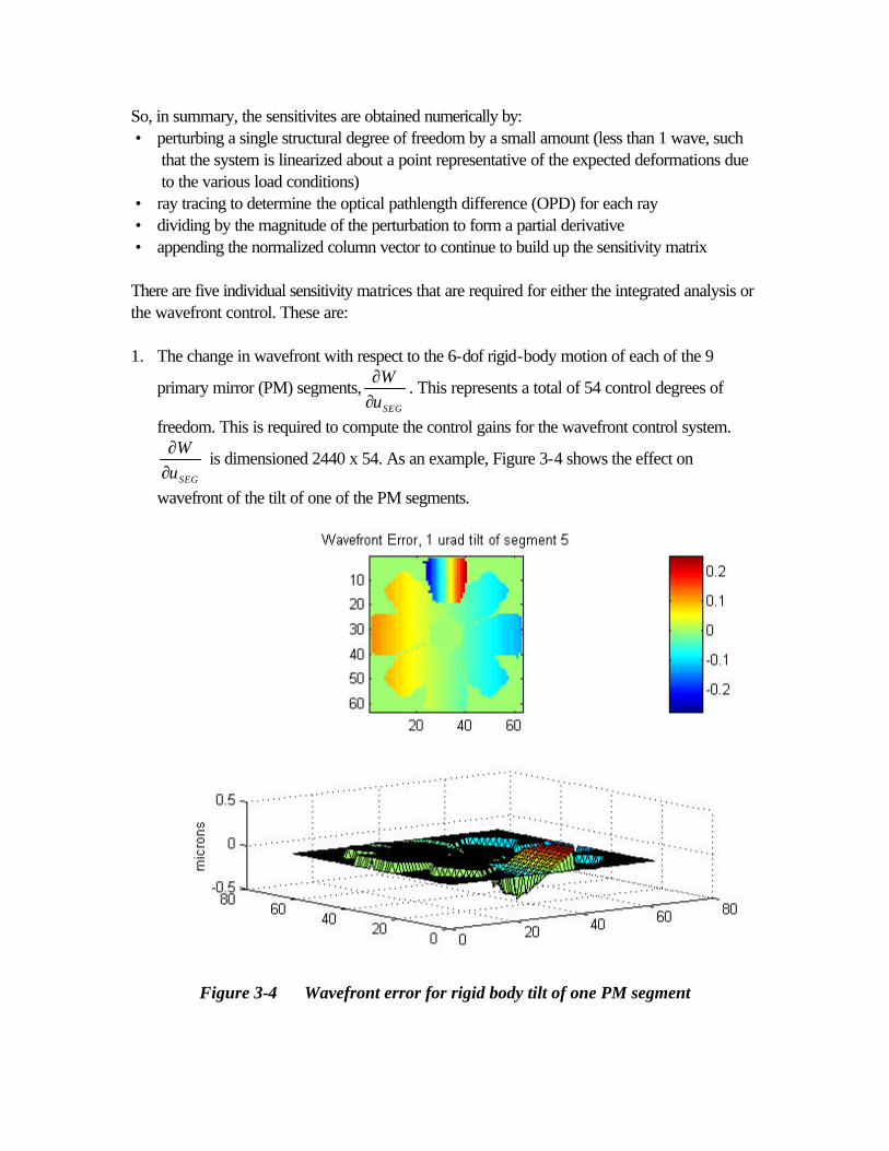
So, in summary, the sensitivites are obtained numerically by: • perturbing a single structural degree of freedom by a small amount (less than 1 wave, such

that the system is linearized about a point representative of the expected deformations due to the various load conditions)

• ray tracing to determine the optical pathlength difference (OPD) for each ray • dividing by the magnitude of the perturbation to form a partial derivative • appending the normalized column vector to continue to build up the sensitivity matrix There are five individual sensitivity matrices that are required for either the integrated analysis or the wavefront control. These are: 1. The change in wavefront with respect to the 6-dof rigid-body motion of each of the 9

primary mirror (PM) segments,SEGu

W

∂∂

. This represents a total of 54 control degrees of

freedom. This is required to compute the control gains for the wavefront control system.

SEGu

W

∂∂

is dimensioned 2440 x 54. As an example, Figure 3-4 shows the effect on

wavefront of the tilt of one of the PM segments.

Figure 3-4 Wavefront error for rigid body tilt of one PM segment

2. The change in wavefront with respect to the change in stroke of each of the 349 actuators in

the deformable mirror (DM), DMu

W

∂∂

. This is required to compute control gains for the

wavefront control system. DMu

W

∂∂

is dimensioned 2440x349. As an example, Figure 3-5

shows the effect on wavefront of a single actuator poke. The DM is modeled using influence functions to compute surface height and slope as functions of actuator stroke. The influence

functions used in this model are of the form 0

sin( )sin( )( , )

x yz x y Z

x y= where z is the

surface height as a function of distance (x,y) from the actuator location. This form was found [5] to be a reasonable approximation based on previous measurements of similar mirrors.

Figure 3-5 Wavefront Error for a single DM Actuator poke 3. The change in image centroid coordinates (x,y) with respect to the 6-dof rigid-body motion

of each of the 19 optical elements, plus the field angle of the source and the control

actuation (gimbal) angles of the fast steering mirror, RBu

C

∂∂

. This is required for the jitter

analysis. In the jitter model, the ISIM, including all mirrors in the optical train after the secondary mirror and the NIR camera, is assumed to be infinitely stiff. Therefore, only 66 dofs – 6 for each of the 9 PM segments, 6 for the SM, and 6 for the ISIM/NIRCAM – are

required rather than 114. The addition of the field angle dofs – the source moves in the optical frame as the inverse of the observatory motion in the inertial frame – and the FSM

actuation result in a matrix RBu

C

∂∂

that is dimensioned 2x71. As noted [4], these most critical

of these sensitivites are relatively easy to compute analytically. 4. The change in wavefront with respect to the 6-dof rigid-body motion of each of the 19

optical elements, plus the field angle of the source and the control actuation (gimbal) angles

of the fast steering mirror ,RBu

W

∂∂

. This is required for the jitter analysis, and again, as the

ISIM/NIRCAM is modeled as a single rigid element in the jitter model, there are a total of

71 dofs and RBu

W

∂∂

is dimensioned 2440 x 71.

5. The change in wavefront, with tilt removed, with respect to flexible body 3-dof translations of the FEM grid points on the surface of the PM, plus the 6-dof rigid-body displacements

of the SM and ISIM/NIRCAM, FEMu

W

∂∂

. This is required for the thermal stability analysis.

There are 344 grid points in the FEM located on the PM surface, so this represents a total

of 1044 structural degrees of freedom. FEMu

W

∂∂

is dimensioned 2440 x 1044. As an

example, Figure 3-6 shows the effect on wavefront due to a 1 micron X-translation of FEM node 188. Unlike the DM, this effect is not modeled using analytic influence functions. Rather, an internal algorithm in MACOS is used to interpolate the surface elevation and slope at the ray intercepts as a function of the (x,y,z) coordinates of the FEM grid points.

Figure 3-6 Wavefront error due to 1 micron x-translation of FEM node

4. Thermal Models Two thermal models were used for the integrated analysis. One is a system-level model of the entire observatory, shown in Figure 4-1, including the sunshield, SSM, ISIM, and OTA. This model was used to determine the effect of boundary conditions upon the OTA bulk temperature, largely in support of sunshield design trades.

Figure 4-1 OTA thermal model with ISIM (11/97 Baseline), beryllium primary mirror and seconday mirror mast, and open reaction structure

In the system model, the OTA includes a beryllium primary mirror, support structure, and secondary mirror mast. The support structure is open, exposing the back surface of the mirror to the sunshade and the ISIM. The beryllium mirror petals are 2 mm thick and are supported on the beryllium reaction structure by titanium actuator pins at three locations per petal. The primary mirror support structure is modeled radiatively using TRASYS (Thermal Radiation Analysis SYStem) cylinders [6]. Radiative exchange from the struts supporting the secondary mirror is also included. The second model is of the OTA only, with more detail added such as the conductive paths through the structural elements in the primary mirror support structure and the secondary mirror mast. Surfaces representing the sunshade, SSM, and ISIM are treated as boundary nodes with temperatures that are inherited from the system level analyses[7]. The back side (facing the OTA) of the sunshade is highly reflective, with an infrared emittance of 0.03, and the surfaces of the ISIM radiate with an infrared emittance of 0.70. All steady state analyses were conducted for the worst case “hot attitude” where the sunshade normal is coincident with the sun vector. A

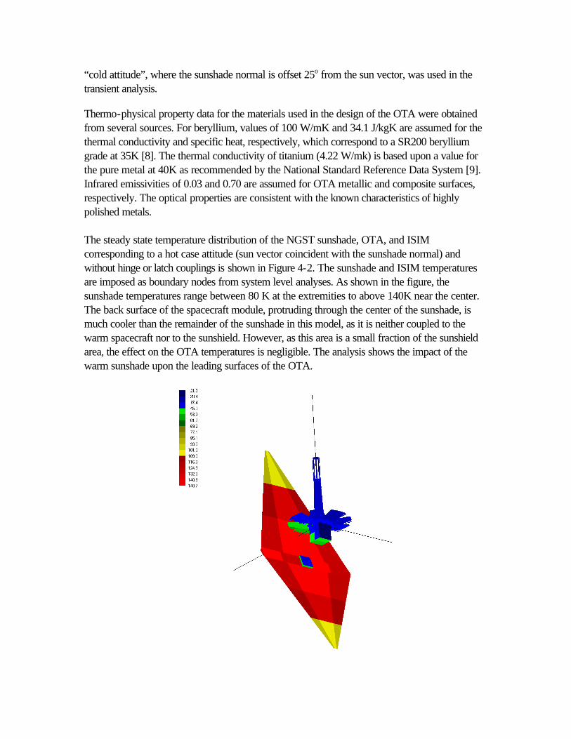
“cold attitude”, where the sunshade normal is offset 25o from the sun vector, was used in the transient analysis.

Thermo-physical property data for the materials used in the design of the OTA were obtained from several sources. For beryllium, values of 100 W/mK and 34.1 J/kgK are assumed for the thermal conductivity and specific heat, respectively, which correspond to a SR200 beryllium grade at 35K [8]. The thermal conductivity of titanium (4.22 W/mk) is based upon a value for the pure metal at 40K as recommended by the National Standard Reference Data System [9]. Infrared emissivities of 0.03 and 0.70 are assumed for OTA metallic and composite surfaces, respectively. The optical properties are consistent with the known characteristics of highly polished metals. The steady state temperature distribution of the NGST sunshade, OTA, and ISIM corresponding to a hot case attitude (sun vector coincident with the sunshade normal) and without hinge or latch couplings is shown in Figure 4-2. The sunshade and ISIM temperatures are imposed as boundary nodes from system level analyses. As shown in the figure, the sunshade temperatures range between 80 K at the extremities to above 140K near the center. The back surface of the spacecraft module, protruding through the center of the sunshade, is much cooler than the remainder of the sunshade in this model, as it is neither coupled to the warm spacecraft nor to the sunshield. However, as this area is a small fraction of the sunshield area, the effect on the OTA temperatures is negligible. The analysis shows the impact of the warm sunshade upon the leading surfaces of the OTA.

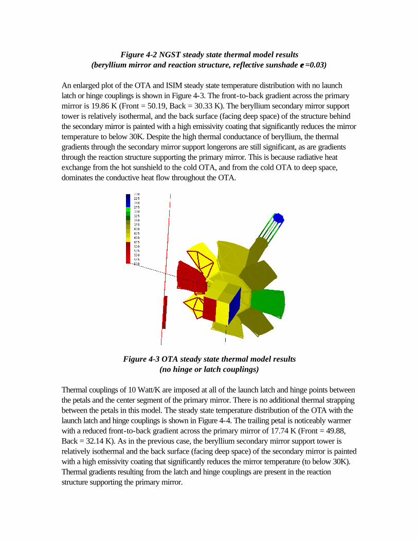
Figure 4-2 NGST steady state thermal model results (beryllium mirror and reaction structure, reflective sunshade εε =0.03)

An enlarged plot of the OTA and ISIM steady state temperature distribution with no launch latch or hinge couplings is shown in Figure 4-3. The front-to-back gradient across the primary mirror is 19.86 K (Front = 50.19, Back = 30.33 K). The beryllium secondary mirror support tower is relatively isothermal, and the back surface (facing deep space) of the structure behind the secondary mirror is painted with a high emissivity coating that significantly reduces the mirror temperature to below 30K. Despite the high thermal conductance of beryllium, the thermal gradients through the secondary mirror support longerons are still significant, as are gradients through the reaction structure supporting the primary mirror. This is because radiative heat exchange from the hot sunshield to the cold OTA, and from the cold OTA to deep space, dominates the conductive heat flow throughout the OTA.

Figure 4-3 OTA steady state thermal model results (no hinge or latch couplings)

Thermal couplings of 10 Watt/K are imposed at all of the launch latch and hinge points between the petals and the center segment of the primary mirror. There is no additional thermal strapping between the petals in this model. The steady state temperature distribution of the OTA with the launch latch and hinge couplings is shown in Figure 4-4. The trailing petal is noticeably warmer with a reduced front-to-back gradient across the primary mirror of 17.74 K (Front = 49.88, Back = 32.14 K). As in the previous case, the beryllium secondary mirror support tower is relatively isothermal and the back surface (facing deep space) of the secondary mirror is painted with a high emissivity coating that significantly reduces the mirror temperature (to below 30K). Thermal gradients resulting from the latch and hinge couplings are present in the reaction structure supporting the primary mirror.

Figure 4-4 OTA steady state thermal model results (conductive hinge and latch couplings)

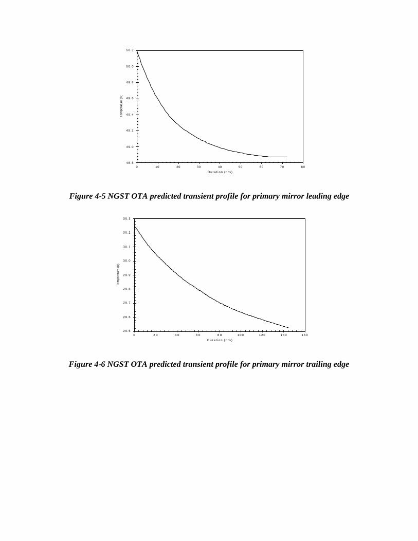
The transient response of the leading (closest to the sunshade) and trailing edges of the primary mirror are provided in Figures 4-5 and 4-6. The initial condition is the steady state temperature of the OTA and sunshade corresponding the sun perpendicular to the sunshield. In the transient analysis, the spacecraft is slews to the maximum pitch angle of 25o, which represents the cold case. Because the settling time of the OTA is very large compared to the duration of the slew, it is assumed that the slew is instantaneous. The results are not dependent upon the direction of the slew for two reasons: (1) the OTA orientation is fixed relative to the sunshade, and (2) the solar flux incident upon the front surface of the sunshade is determined only by the cosine of the angle between the sunshade normal and the incident sun vector. To simulate the thermal transient response for a slew, the temperatures of the OTA nodes were initialized using the ground-to-orbit steady-state results, which is the same as the “hot attitude”. Next, the temperatures of the sunshield nodes were initialized using the steady-state results with the sunshield at the maximum pitch angle to the sun. These boundary node temperatures were then held constant during the transient. To the OTA, it was as if an instantaneous step-change was applied to the radiatively-coupled boundary nodes. Figures 4-5 and 4-6 show the temperatures of the leading and trailing edges, respectively, of the primary mirror as functions of time. The temperature of the leading edge approaches a new steady-state value of 48.8K, a decrease of 1.4 K from the initial condition, after 70 hours. However, even after twice that duration, or 140 hours, it is apparent that the temperature of the trailing edge has yet to approach a new steady-state value. At that time, the temperature of the trailing edge has fallen to 29.5 K, a decrease of 0.7K from the initial condition.

48 .8

49 .0

49 .2

49 .4

49 .6

49 .8

50 .0

50 .2

0 10 20 30 40 50 60 70 80

D u r a t i o n ( h r s )

Tem

pera

ture

(K

)

Figure 4-5 NGST OTA predicted transient profile for primary mirror leading edge

29 .5

29 .6

29 .7

29 .8

29 .9

30 .0

30 .1

30 .2

30 .3

0 2 0 4 0 6 0 8 0 1 0 0 1 2 0 1 4 0 1 6 0

D u r a t i o n ( h r s )

Tem

pera

ture

(K

)

Figure 4-6 NGST OTA predicted transient profile for primary mirror trailing edge

5. Pointing Control System Model The pointing control system [10] consists of multiple control loops for inertial attitude and line-of-sight stabilization, plus a vibration isolation stage to attenuate the high-frequency dynamic forces and torques produced by the effects of reaction wheel rotor imbalances and bearing irregularities. This section describes the controller, sensor, actuator, and disturbance models. 5.1 Attitude Control System Gyros and star trackers are used as sensors for attitude determination. Attitude is represented as a quaternion; the quaternion is propagated using angular rate data from a 3-axis inertial reference unit (IRU, or rate-gyro) sampled at a 10 Hz rate. The star trackers (ST) are sampled at a 2 Hz rate; these direct inertial attitude measurements are optimally combined with the gyro-propagated attitude via a Kalman filter. Reaction wheels, located in the SSM, provide torques to steer the observatory. There are 4 wheels arranged in a pyramid-like geometry; all wheels are actively controlled to provide the 3-axis control. This allows an extra degree-of-freedom in the controller used to bias the mean wheel speed to a desired set point. This feature may be exploited to avoid structural resonances or to maximize bearing lifetime. The 3-axis torque commands are developed via a digital controller consisting of three decoupled PID contollers in series with lowpass filters for flexible mode attenuation. A block diagram of the attitude control system (ACS), taken from the SimulinkTM time-domain simulation model, is shown in Figure 5-

1. Figure 5-1 ACS block dagram

gyro

WheelsStructural Filters

tracker

PID Controllers

K

EstimatedInertia Tensor

AttitudeDetermination

CommandRate

CommandPosition

Forces &Torques

PID bandwidth is 0.025 Hz

3rd order LP elliptic filters for flexiblemode gain suppression

Kalman Filter blends 10 Hz IRU and 2 Hz STdata to provide optimal attitude estimate

Wheel model includes non-linearitiesand imbalance disturbances

The Kalman filter used for attitude determination traces its heritage to Landsat [11] and has been refined on subsequent missions such as XTE [12]. This filter assumes that the attitude (star tracker) and rate (gyro) measurements are corrupted by white noise, and furthermore that the rate measurements are corrupted by a random walk component (rate bias, or gyro drift). The measurement models are given by

where ω is the rate, b is the rate bias, θ is the angle, and the η’s are random processes. Discrete-time versions of these models are implemented in the simulation. The inputs to the Kalman filter are the residuals, or differences, between the measured and expected positions of guide stars. The model contains a star catalog to implement this feature. The outputs of the filter are estimated errors in the inertial attitude estimate (roll, pitch and yaw angle updates) and in the rate bias estimate (roll, pitch and yaw gyro drift updates). The predicted performance of this attitude determination system can be found by iterating the filter equations to steady-state. Although precise estimates of the filter performance require numeric simulation or covariance analysis, a useful design tool may be employed to make a first cut at key filter parameters. An analytic solution was found [13] for the case a single-axis estimation problem, where the standard deviations of the attitude and rate bias estimates are given by

where Tu is the Kalman filter update rate (star tracker sample rate) and the other parameters are the standard deviations of the measurement noise processes given above. Given model parameters for the Kearfott IRU flown on XTE (σv = 0.01 arcsec/second1/2, σu = 7x10-5 arcsec/second3/2) and the specifications for the new Lockheed AST301 star tracker (σn = 1.35 arcsec/star/sample), the above solution is used to set the 2 Hz star tracker update rate. A numerical simulation of the Kalman filter established steady-state standard deviations of 0.3, 0.4, and 0.4 arcseconds, 1σ, in roll, pitch, and yaw respectively. The NGST integrated simulation features a switch to disable the Kalman filter and simply inject noise with the above values into the position channel of the controller. This feature is provided to improve simulation speed at the expense of (negligible) fidelity.

)noisewhiteangle(),0(~ˆ

)walkrandombias(),0(~

)noisewhiteratebias,rate(),0(~ˆ

nnn

uuu

vvv

b

b

σηηθθ

σηη

σηηωω

+=

=

++=&

( )( ) 4121221

412122141

2

2

unuvu

unuvnu

T

TT

σσσσω

σσσσθ

+=∆

+=∆

The discrete-time, single-axis PID controller equations are of the following form

where θ is position (subscripts stand for “command” and “error”); KP, KI, and KD are the proportional, integral, and derivative gains, respectively; Ts is the sample period; and z is the shift operator. The controller operates at the gyro sampling rate of 10 Hz. Command accelerations are developed using the above expression for the roll, pitch, and yaw channels. The PID gains, KP, KI, and KD, are defined as follows:

For the current yardstick design, all three axis use identical parameters: fc = 0.025 Hz, fa = 0.075, ζc = 0.7071. The command accelerations and command torques to the reaction wheels, are 3x1 vectors containing commands for the roll, pitch, and yaw channels, i.e.

The command torque is developed via use of the estimated inertia matrix (I), as shown by the following expression:

This treatment is necessary for designs such as NGST in which there are significant cross-products of inertia. A completely decoupled design would be insufficient for such a structure, but might suffice for more symmetric designs.

errDerrs

IerrPcmd Kz

TKK θθθθ &&& +

++=

1

constantstimeintegral-to-PDofratio

ratiodampingcontroller

(hz)bandwidthcontroller

(rad/sec)bandwidthcontroller2

where

)2(

)12(3

22

===

==

+==

+=

a

c

c

cc

accD

cacI

cacP

f

f

f

fK

fK

fK

ζ

πω

ζωζω

ζω

cmdcmd I θτ &&~=

=

=

z

y

x

cmd

z

y

x

cmd and

τττ

τθθθ

θ&&&&&&

&&

The roll, pitch, and yaw command torques are filtered via discrete-time elliptic lowpass filters. These filters are designed directly via MatlabTM Signal Processing Toolbox commands. For the yardstick design, the roll, pitch, and yaw filters have identical parameters: 3rd order filters with a 0.15 Hz corner, 3db passband ripple, and 35 dB stopband attenuation. The tuning of the controller is fairly straightforward. The PID gains are set such that the gain margin is at least 12 dB and the phase margin is at least 30 deg. This is done using only rigid body dynamics in the plant model. Following the PID gain selection, the flexible body dynamics are added to the plant, and the cutoff frequencies and orders of the elliptic lowpass filters are determined such that the closed-loop system is gain-stabilized by at least 10 dB. Table 5-1 gives the results for the current NGST design. Note that the addition of the lowpass filters has reduced the rigid body upper gain margins and phase margins below the design goals. Through additional tuning of the filter parameters it is possible to completely satisfy these goals, but at this preliminary design stage these margins are sufficient to proceed to the next step, time-domain simulations to predict performance.

Modal Axis

Lower Gain Margin (dB)

Upper Gain Margin (dB)

Phase Margin (deg)

Flexible Mode Gain Suppression (dB)

1 25 @0.0065 hz 10.4 @0.09 hz 22 @0.035 hz 40 @0.42 hz 2 25 @0.0063 hz 10.5 @0.09 hz 22 @0.035 hz 30 @0.51 hz 3 25 @0.0063 hz 10.3 @0.09 hz 22 @0.035 hz 30 @1.1 hz

Table 5-1 ACS Controller Stability Margins

There is a final stage to the controller. NGST features a 4-wheel design, but the controller to this point has developed only 3 commands, in body frame. To command the wheels, the pseudo-inverse of the wheel-to-body transformation matrix is used to transform the 3-vector into a 4-vector. The additional degree-of-freedom is controlled by applying a constraint which is used to set the (approximate) mean wheel momentum. The 4 –vector of wheel torque commands is then given by an expression of the form

where wheelAbody is the 4x3 wheel-to-body transformation matrix, K is some (small) constant gain, and Hmax and Hmin are the maximum and minimum wheel momenta, respectively.

1 max min

0 0 0

0 0 0

0 0 0 20 0 0

whl wheel body cmd

K

K H HA

K

K

τ τ−

+ = +

5.2 Reaction Wheel Dynamics and Vibration Isolation The ACS block includes the reaction wheel disturbance model. The current model neglects all disturbances except for in-plane forces and torques arising from static and dynamic imbalance. A simplfied physical model [14] of this phenomenon is shown in Figure 5-2. In this model, the disturbances are assumed to arise from small concentrated masses located on the wheel rotor. A single small mass located on the mid-plane of the rotor, as shown on the left, produces a force acting outward in the radial direction that is proportional to the wheel speed squared. Similarly, two small masses located opposite one another on the rotor, but separated by a distance d along the spin axis (Z), will produce a moment about an axis in the radial direction. Again, the magnitude of this moment is proportional to the wheel speed squared. Both the force vector and moment vector precess as the wheel rotates.

Figure 5-2 Wheel imbalance physical model These forces (F) and torques (T) are modeled as summations of sinusoidal terms -- the fundamental component at wheel speed plus some number of harmonic and sub-harmonic terms related to bearing geometry. Equations for this model take the following form as functions of time (t), parameterized in terms of wheel speed (ω), a random phase angle (φ) static and dynamic imbalance coefficients (Us and Ud), harmonic coefficients (ai), and harmonic speed ratios (hi).

)cos()(

)sin()(

)cos()(

)sin()(

1

2

1

2

1

2

1

2

φωω

φωω

φωω

φωω

+=Τ

+=Τ

+=

+=

∑

∑

∑

∑

=

=

=

=

thaUt

thaUt

thaUtF

thaUtF

i

n

iidx

i

n

iidx

i

n

iisy

i

n

iisx

Static Imbalance Dynamic Imbalance

ωω

F

F

d

r

m

mωω

F

r

m

Us = mrF = Us

ωω2Ud = mrdT = Ud

ωω2

YZ

X X

Y

Z

The parameters for the above expressions used in the NGST model, provided in [15], are taken from measurements on wheels for HST. Similar measurements have been taken on Ithaco wheels, and other sources are being explored to enlarge the database of wheel disturbance models for subsequent analysis. Using the above model, A representative plot of wheel force power spectral density is shown in Figure 5-3, for one axis of a single wheel running at 1200 rpm (20 Hz). The PSD plot clearly highlights the harmonic nature of the signal

Figure 5-3 Wheel force power spectral density The vibration isolation model is a highly simplified model of a reaction wheel isolation system similar to that discussed in [16,17]. At this time, the isolator is simply modeled as a set of 6 parallel, 2nd order, lowpass filters. Such a model is adequate for frequency-domain analysis. A more realistic model would include physical elements in the structural FEM to represent the reaction wheels and the isolator structure (typically a set of struts and dampers arranged in a hexapod configuration for 6-dof isolation). A transfer function for this simple filter model is of the form

The parameters ω0 and ζ0 define the characteristics of this filter; ω0 is the natural frequency, and ζ0 is the damping. Devices employed in this application may be classified as passive (mechanical spring/damper), hybrid (passive plus electromechanical servo), or active (magnetic suspension). Reasonable assumptions for natural frequency and damping of the filter depend on the device type assumed. Passive devices will exhibit lower damping, typically less than 5-10%, and natural frequencies generally 5 Hz or greater. Hybrid and active devices may be tuned to achieve higher damping, perhaps as high as 50%, and lower natural frequencies, perhaps as low as 0.1 Hz. However, sensor noise and actuator non-linearities will combine to limit performance of these devices.

( ) 2000

2

20

2 ωωζω

++=

sssG

N 2/Hz

0 5 0 1 0 0 1 5 0 2 0 0 2 5 00

0 . 0 1

0 . 0 2

0 . 0 3

Hz

Figure 5-4 shows two representative transfer functions. One represents a 10 Hz, 5 % damped passive suspension; the second represents a 1 Hz, 40% damped hybrid device with ideal

feedback sensors (no noise floor at high frequencies). Figure 5-4 Typical vibration isolator response functions

5.3 Line-of-Sight Stabilization System Line-of-sight stability is required at the milli-arcsecond level, but the ACS only provides arcsecond level performance. The addition of a two-axis gimbaled, reactionless, fine steering mirror controller provides the additional attenuation at low frequencies. The feedback sensor for this control loop is the NIR camera. A dedicated sub-window of the 4' x 4' FOV will be processed to extract pitch/yaw pointing errors for guide stars. The guide star detector model assumes that the sensor error is essentially due to photon noise. It can be characterized as having a Noise Equivalent Angle that is a function of the detector read noise and quantum efficiency, telescope diameter and throughput, wavelength, and guide star magnitude. The total number of photons collected depends on the detector integration time.

In this expression, k is the slope of the centroiding function and is given by

which assumes that the image is a perfect Airy function.

NEA

RN

k N=

+1 0

kD

=163πλ

1 0-2

1 0-1

1 00

1 01

1 02-200

-150

-100

- 5 0

0

5 0

d B

Hz

Magn i tude Response

1 H z H y b r i d D e v i c e

1 0 H z P a s s i v e D e v i c e

Furthermore, we assume the following values for the remainder of the parameters required:

R0 (detector readout noise over 4 pixels) = 4 * (30 electrons)2 D (telescope diameter) = 8 m λ (wavelength) = 2.2 microns N (total number of detected photons) = (ε)(Qe)(πD2/4)(BP)(10-0.4M)(Φ)(TI) ε (throughput) = 0.6 Qe (quantum efficiency) = 0.8 BP (bandpass) = +/- 25% M (guide star magnitude) = 16.5 Φ (total photon flux) = 3.6x1010 photons/m2/micron/sec and TI is the integration time (TBD)

Figure 5-5 shows the sensor noise, in milli-arcseconds, as a function of integration time. To meet a requirement of 5 mas (1σ), allocating no more than 50% of this error to sensor noise, we see that a integration time of at least 0.025 sec (max. 40 Hz sample rate) is required.

Figure 5-5 NEA vs. Integration Time

A discrete-time noise model was developed , allowing the integration time to be varied and appling the correct amount of noise to the X and Y coordinates of the image centroid. Figure 5-6 shows sample time histories of this noise model.

0.01 0.02 0.03 0.04 0.05 0.06 0.07 0.08 0.09 0.1 0.112

2.2

2 .4

2 .6

2 .8

3

3.2

3 .4

3 .6

3 .8

s e c

m a s

B a s e l i n e i s 3 0 H z s a m p l e r a t e

1 σσ L O S r e q u i r e m e n t i s 5 m a s

Figure 5-6 GS Noise Model Representative Time Responses

The FSM model was derived from transfer function data taken from an off-the-shelf design [18]. The poles and zeros were scaled from the nominal 2200 Hz rate to the 30 Hz rate set by the guide star noise. A simplified, single-axis representation of the FSM system is shown in Figure 5-7.

Figure 5-7 FSM Servo Loop Single-axis Block Diagram

0 1 2 3 4 5 6 7 8 9 1 0- 1 0

-5

0

5

1 0G S X A x i s N o i s e , s t d = 2 . 5 2 8 7 m a s

m a s

0 1 2 3 4 5 6 7 8 9 1 0- 1 0

-5

0

5

1 0G S Y A x i s N o i s e , s t d = 2 . 5 1 5 7 m a s

s e c

m a s

ZMIR

PMIR

CS

++

+

-

+

+

+

θO T A

θR E F

θ MIR

ηGS

θ L O S

The following transfer functions result from the scaled measurements of the LHDC FO50-35 FSM.

The two most important closed-loop transfer functions that can be derived for this system are from guide star noise to LOS error, and from base motion to LOS error. Expressions for these transfer functions are given by

Plots of these transfer functions are given in Figure 5-8, showing that the FSM servo acts as a low-pass filter to guide star noise, and as a high-pass filter to base motion. The effective bandwidth of this controller is approximately 2 Hz. Figure 5-9 shows the result of the lowpass filter action on the guiding sensor noise time histories shown in Figure 5-6. This important result represents a limit on LOS performance, which is referred to as the guide star noise floor. In the absence of all other disturbance sources, this is the best we can do for this design. The LOS error is seen to be 2 mas, compared to a 1-σ requirement of 5 mas. Assuming all other errors add in quadrature, this results in an allocation of 4.6 mas to all other sources – principally, the un-attenuated rigid and flexible body motion of the telescope and optics.

)120 ofion magnificat optical includes(1000

);01.0(2);1.0(2

);0.5(2);4.0(2

11

11

11

02.0);100(2

2

43

11

432

1

neglectedbecan

simulationinneglectedis

0

200

2

20

=====

++++=

==++

=

K

ssss

KC

ssP

s

MIRZ

MIRP

MIR

πωπωπωπω

ωωωω

ζπωωζω

ω

MIRsOTA

LOS

MIRs

MIRs

GS

LOS

PC

PC

PC

+=

+=

11

1

θθηθ

Figure 5-8 FSM Transfer Functions

Figure 5-9 Guide Star Noise Floor set by FSM Lowpass Filter Action

0 1 2 3 4 5 6 7 8 9 1 0- 1 0

- 5

0

5N I R X C e n t r o i d , s t d = 1 . 8 4 7 3 m a s

m a s

0 1 2 3 4 5 6 7 8 9 1 0- 1 0

- 5

0

5

1 0N I R Y C e n t r o i d , s t d = 2 . 0 8 3 8 m a s

s e c

m a s

1 0-4

1 0-2

1 00

1 02

1 04

- 6 0

- 5 0

- 4 0

- 3 0

- 2 0

- 1 0

0

1 0

Hz

d B

Acts as a high-passfilter to base-motion

Acts as a low-passfilter to guide star noise

6. Integrated Structural-Thermal-Optical Model and Analysis Operation at cryogenic temperature presents a major challenge for NGST, and one of the main areas of concern is here in the thermal deformation of the optics as they go from the ambient environment to on-orbit conditions. This section addresses the changes that the Yardstick experiences as it cools, and then again, as it changes attitude during observations. Mathematically, the thermal model takes the form

[ ]∑+

=

−+−−=bq NN

jijijijiji TTRTTCQ

1

44 )()(

where Ti,j = (T1,T2,T3,…,TNq) is the temperature vector (state) of the system Nq is the number of diffusion nodes Nb is the number of boundary nodes Qi = (Q1,Q2,Q3,…,QNq) is the vector of heat inputs to the system Ci,j are the conduction coefficients of the system Ri,j are the radiation coefficients of the system Using SINDA or IMOS or some other numerical solver, the above thermal network equations are solved to provide the temperatures. The same network model is used for both steady-state and transient cases; however, different numerical solutions are applied in either case. Once the temperatures have been found, a linear model is employed to directly estimate the wavefront error. This model is given by

uwFEMu

W

∂∂=

where w is the wavefront error (OPD) vector, FEMu

W

∂∂

is the optical sensitivities w.r.t. flexible-

body displacements of the OTA as detailed in section 3, and u is the vector of displacements. In turn, the displacements are given by

)~~

( 0TTFKu −=

where K is the pseudo-inverse of the stiffness matrix, F is the temperature-to-force transformation (a function of material CTE), and 0

~T and T~ are the initial (zero-stress) and final

temperatures for the subset of thermal nodes corresponding to nodes in the structural model.

Wavefront error is generally expressed as an RMS value, given by

wwTWFE =σ

The previous expressions may be combined to give a direct relationship between nodal temperatures and scalar RMS wavefront error

)~~

()~~

( 00 TTCTT −−= TWFEσ

where C is a square matrix given by

T

FEMFEM u

W

u

W))(( FKFKC

∂∂

∂∂=

6.1 Steady-State Performance Figure 6-1 indicates the temperatures expected in operation at L2. It is seen that the sunshield passively cools the PM segments to temperatures ranging from 52 K on the petal facing the sunshield and SSM, down to 30 K on the petal facing deep space.

Figure 6-1 OTA steady-state temperatures

NGST will employ cryo-null figuring techniques to establish the final figure of the optics. This process involves testing at near-operational temperatures, along with room temperature polishing, to achieve final figure. At room temperature, the segments will have figure errors built in to compensate for the distortion that occurs during cooling. As the temperature during testing

X

Y

Z

52.84

49.54

46.24

42.93

39.63

36.33

33.03

29.72

26.42

23.12

19.82

16.51

13.21

9.908

6.605

3.303

0 .

V1

L100

C50

Output Set: temperatures

Contour: Table Output Vector 1

is likely to be around 70-100 degrees K due to practical limitations (liquid Helium vs liquid Nitrogen), the analysis here assumes the zero-stress temperature for the OTA to be a uniform 100 K. Figure 6-2 displays the effect on OPD and PSF when the OTA is cooled from the uniform 100 K to the temperatures shown in Figure 6-1. The initial WFE is 46 microns RMS. This error is sensed by the wavefront sensor, which utilizes a phase-diversity approach. Next, control is applied to the segment and deformable mirror actuators to achieve diffraction limited performance. This correction proceeds in several stages, alternating between segment and DM control, each stage involving a small number of iterations. After segment-only WF control in 3DOF, the initial error is reduced to 240 nm. Most of this control has acted to counter “rigid-body” motions of the segments resulting from distortions in the reaction structure. The DM is effective in restoring full performance. Without DM actuator stroke limits in the model, the WFE approaches 25 nm! However, the actuator stroke limit (1.8 um) limits the error to 77 nm.

Figure 6-2 Ground-to-orbit thermal performance, pre- and post-control 6.2 Thermal Transient Performance Using the transient temperature results given in section 4 with the integrated model, we see that significant degradation of the image occurs immediately during a slew. Furthermore, given the long thermal time constant for the system, the image quality continues to degrade long after the slew has ended.

On-Orbit Thermal

Wave

front

WFE=4.6271e-05

20 40 60 80 100

20

40

60

80

100

Ima

ge

Strehl=0.0061111

20 40 60 80 100 120

20

40

60

80

100

120

After Segment Control

WFE=2.3886e-07

20 40 60 80 100

20

40

60

80

100

Strehl=0.60555

20 40 60 80 100 120

20

40

60

80

100

120

After DM Control

WFE=2.4702e-08

20 40 60 80 100

20

40

60

80

100

Strehl=1.0117

20 40 60 80 100 120

20

40

60

80

100

120

Limited DM Control

WFE=7.7059e-08

20 40 60 80 100

20

40

60

80

100

Strehl=0.96472

20 40 60 80 100 120

20

40

60

80

100

120

The initial temperatures correspond to the “hot attitude”. At this point, it was assumed that the wavefront contol system had been applied to set an excellent initial figure quality (σWFE = 20 nm, Strehl = 0.99). Again, as detailed in section 4, an instantaneous change was applied to the temperatures of the sunshield nodes, using the “cold attitude” steady state values. The OTA then begins to cool, and the mirrors, reaction structure, and other supporting structure all begin to deform. The model computes the deformations and the OPD at each time step. After 28 hours, figure quality has been reduced significantly (σWFE = 322 nm, Strehl = 0.72), as seen in Figures 6-3, 6-4 and 6-5.

Figure 6-3 Thermal transient performance

0 5 10 15 20 25 300

1

2

3

4x 10

-7 Wavefront Error vs. Time

Time (hr)

WF

E R

MS

(m

)

0 5 10 15 20 25 300.7

0.8

0.9

1

Strehl Ratio vs. Time

Time (hr)

Str

eh

l

-10

-9

-8

-7

-6

-5

-4

-3

-2

-1Initial image (log-intensity)

20 40 60 80 100 120

20

40

60

80

100

120 - 0 . 0 4

- 0 . 0 3

- 0 . 0 2

- 0 . 0 1

0

0 . 0 1

0 . 0 2

0 . 0 3

0 . 0 4

0 . 0 5

In i t i a l OPD a t ex i t pup i l , m ic rons

20 40 60 80 1 0 0

10

20

30

40

50

60

70

80

90

1 0 0

1 1 0

Figure 6-4 Initial image (log-intensity) and OPD

-8

-7

-6

-5

-4

-3

-2

Final image (log-intensity)

20 40 60 80 100 120

20

40

60

80

100

120-0.6

-0.4

-0.2

0

0.2

0.4

0.6

Final OPD at exit pupil, microns

20 40 60 80 100

10

20

30

40

50

60

70

80

90

100

110

Figure 6-5 Final image (log-intensity) and OPD

6.3 Compensation via Active Thermal Control Even after the most extreme thermal transient, as shown in the above example, the final figure error is well within the capability of the wavefront sensing and control system to correct. However, in order to preserve science operations efficiency, it is desirable that it not be necessary to repeat this lengthy procedure after maneuvers large enough to produce such significant image degradation. One approach [19], developed using the integrated models, involves the use of heaters on the OTA, providing continuous compensation for the time-varying heat loads from the sunshield. The linear model that maps temperature to wavefront error provides a means to perform a non-linear optimization that enables selection of desirable heater locations on the OTA, and to then calculate the required output of each heater. Two alternatives were examined: (a) the cost function was chosen to minimize the change in temperature of the nodes where the heaters were located, and (b) the cost function was chosen to minimize the change in wavefront error. The first approach results in a design in which the temperature change over some portion (the reaction structure being the optimum location for the heaters) of the OTA is small, but which

only indirectly minimizes the change in wavefront error. The second approach directly minimizes the change in wavefront error, although it allows the temperatures at the heater nodes to drift somewhat.

Figure 6-6 OPD without active thermal control (left), with temperature control

(middle), and with wavefront control (right) Figure 6-6 shows that the two control alternatives produce roughly equivalent results in terms of post-control wavefront error. However, option (b) requires significantly less heater power in order to obtain this equivalent performance. The minimum temperature-change controller requires 0.21 watts of total heater power; the minimum wavefront error controller requires 0.007 watts of total heater power. This is because the latter approach results in heater power being applied largely where it has the most dramatic effect on wavefront. Figures 6-7 and 6-8 help to illustrate this. Figure 6-7 shows the initial and final temperature distributions, plotted against the node numbers in the thermal model. The grouping of node numbers in the model is apparent in the structure of this distribution, and key groupings are labeled accordingly. In Figure 6-8, the difference (hot-cold) is plotted for three cases: (a) with no control, (b) with temperature control, (c) with wavefront control. For case (b), the figure shows that it is possible to hold most of the structure to within a few tenths of a degree of the initial temperature, thus maintaining good figure quality. However, the figure shows that for case (c), applying heat only at select, highly sensitive locations results in the temperatures over much of the OTA remaining essentially unchanged. It must be noted that either approach requires that the linear model be very accurate. This, in turn, leads to a requirement to perform an initial model update during observatory calibrations,

followed by periodic updates as on-orbit performance data is taken during the lifetime of the observatory.

Figure 6-7 Initial (hot) and final (cold) OTA temperatures plotted by model node #

Figure 6-8 Post-slew temperature variations without control (blue, solid), with temperature control (red, dashed), and with wavefront control (green, dash-dot)

0 1 0 0 2 0 0 3 0 0 4 0 0 5 0 0 6 0 0 7 0 0 8 0 02 0

2 5

3 0

3 5

4 0

4 5

5 0

5 5

6 0

6 5

7 0

n o d e

H o t a n d C o l d T e m p e r a t u r e D i s t r i b u t i o n s

Cold CaseHot Case

Segment Faces Segment Backs

S M

TowerCentersegment

0 100 200 300 400 500 600 700 800-0.5

0

0.5

1

1.5

2

2.5

node

Te

mp

era

ture

(K

)

Difference between Initial and Final Distributions before and After Control

Before Control

After Control of T

After Control of WFE

7. Integrated Jitter Model and Analysis Results The jitter analysis was developed by combining the models for ACS, vibration isolation, structural dynamics, optics, and LOS control. The ACS model includes the sensor noise sources and the dynamic disturbances of the reaction wheels. Initially, these models were integrated as a time-domain simulation in the Simulink environment. The top-level block diagram from this simulation is shown in Figure 7-1.

Figure 7-1 Integrated jitter model

This diagram illustrates the key feature of the Yardstick pointing control architecture [10], the two cascaded control loops (ACS and LOS). Models for all ACS, vibration isolation, and LOS control blocks were presented in the previous sections, at least in equation or transfer function form. Now we will examine the dynamics. 7.1 Dynamics Model Structural dynamics in the integrated model framework are modeled by separating the equations of motion into rigid and flexible body components, as shown in Figure 7-2. The results are combined to yield the translations, rotations, and angular velocities necessary to simulate the measurements of gyros and star trackers, and to generate the wavefront and centroid errors.

Optics

Wavefront

LOS Control

ExternalTorque

Dynamics

Centroid

ACSCommands

ACS

6 4

3

74

74

2

72

72

72

6

6

33

2

VibrationIsolation

Figure 7-2 Dynamics model combines rigid and flexible body motion The block labeled “Rigid Body” solves Euler’s equations of motion for the system about the center of mass.

where H is the system angular momentum, ΣT is the sum of all external torques, and ω is the angular velocity of the observatory. The resulting angular motion may then be used to compute the rigid-body translations of all grid points in the system by virtue of their known displacement vectors relative to the center of mass. The block labeled “Flex Body” models the flexible dynamics as a linear state-space system.

This system is a set of simultaneous, first-order, linear differential equations in generalized coordinates in which the state vector (X), input vector (U), output vector (Y) are defined as follows:

Yout

Sum

Rigid body

Flex Body

Force/Torque

External disturbance

7 2

7 2

3

7 26

X AX BU

Y CX DU

•= +

= +

12 Nxq

qX

= •

∑ ×−= HTH ω&

where q is the vector of generalized, or modal, coordinates, and N is the number of modes extracted in the eigenanalysis

where fx, fy, fz, τx, τy, τz are the reaction wheel forces and torques

where Y consists of 12 6x1 vectors, the first 11 of which are the 3 linear and 3 angular displacements of optical surfaces (PM segments 1-9, SM, FSM) and are of the form

and the 12th is a 6x1 vector containing the 3 angles and 3 angular velocities sensed by the star trackers and gyros The locations of the nodes in the FEM corresponding to these sensors are shown in Figure 7-3.

The simplifying assumption is made that the mirror petals act as rigid bodies. This is justified by the fact that the mirrors are of the “semi-rigid” type, with natural frequencies greater than 60 Hz. Accordingly, the optics models only rely on knowledge of the motions of the 11 grid points identified in Figure 7-3. These grid points are coincident with the vertices of the segments of the mirrors. These are known as "rotation points" in the MACOS model. And, finally, the system matrices (A,B,C,D) are given by

where N is the number of modes extracted in the eigenanalysis, ω is the vector of natural frequencies, ζ is the vector of modal damping coefficients, and φ is the eigenvector matrix. The subscripts on φ indicate that only the columns of φ associated with the input and output nodes identified in Figure 7-3 are retained for the analysis. It is assumed that the modal damping is

[ ]T

zyxzyx fffU τττ=

[ ]Tacs

TT

fsm

T

sm

T

pm

T

pm

T

pm

T

pm

T

pm

T

pm

T

pm

T

pm

T

pmyyyyyyyyyyyyY

9,8,7,6,5,4,3,2,1,=

[ ]T

zyxzyxopticsy φφφδδδ=

T

zyxzyxacsy

=

•••φφφφφφ

672

2723

,

66

,

3

,

626,

6

22

2

0

0

0

0

0

)2()(

0

3

3

66

x

NxxN

Sirui

xN

Sirui

xN

Soptici

NxNx

Tdofi

Nx

NNxNxNiNxNi

NxNNxN

D

C

B

diagdiag

IA

xN

xN

xN

=

Φ

Φ

Φ=

Φ

=

−−

=ζωω

0.001 for all frequencies. It is straightforward to modify the lower-right block of A to change the damping.

Figure 7-3 FEM nodes for optics and ACS sensors/actuators 7.2 Line-of-sight Controls Model Details of the optics block in Figure 7-1 are shown in Figure 7-4. This diagram shows how the

linear optics models (sensitivity matrices RBu

C

∂∂

and RBu

W

∂∂

) are combined with the dynamics

model, the FSM model, and the NIR guiding sensor model. Translations and rotations of the optics, extracted from the output of the dynamics block for the nodes identified in Figure 7-3, are combined with the FSM gimbal angles to create a 74-DOF vector. This vector maps to wavefront and centroid error vectors, 2440x1 and 2x1, respectively, via the sensitivity matrices. The wavefront error vector is saved for post-processing. The centroid of the image is combined with sensing errors using the NIR detector noise model. This feedback signal provides the guiding commands for the FSM controller. The FSM model then computes the gimbal angles required to track this image and compensate for dynamic tip/tilt LOS errors.

ACS (10291)

ISIM (825)

SM (829)

PM (900-908)

These grid points are locatedat the center of the primary andin a circle with radius 2.8 meters,connected to mirror grid pointsby RBE2 elements

ST, IRU, RWAare co-located

FSM, DM, otheroptics are co-located

Figure 7-4 LOS control model Integrated Linear Systems Model The non-linear, sampled-data simulation model shown in Figure 7-1 can be approximated with the simpler, linear system model representation shown below in Figure 7-5. This model contains four linear state space systems representing the structural dynamics, LOS control, ACS, and vibration isolation blocks of the simulation. These are systems (A1,B1,C1) through (A4,B4,C4), respectively. None of these systems contains a feed-through (D) term. There are three inputs to this system: • ηGS - the noise from the LOS control guiding sensor (NIR camera) • ηKF - the noise from the ACS sensors (IRU and Star Tracker, combined in a Kalman

Filter) • FRW - the reaction wheel dynamic disturbances There are two outputs from this system: • C - the LOS error (centroid) • W - the wavefront error (OPD)

1/m2r

radians to metersNIR

GuidingSensor

K

FSMCoordinateCouplingFSM

Controller

22 2 22

m2r

meters to radians(plate scale)

K

Linear SensitivityMatrix for Centroid

Mux22

72

74

2 Centroid

FSM gimbal angles

from FEM

FSM gimbal angles Centroid

θθ

x

y LOS

cent

FEM

FSM

K

y

y

é

ë

ê

ù

û

ú =é

ëê

ù

ûú

WavefrontK

Figure 7-5 Linear systems model for jitter analysis The dynamics include all flexible modes plus the six rigid body modes. The linear optics models, i.e. the sensitivity matrices, are partitioned into two blocks as follows:

where K12 and K22 are the sub-blocks corresponding to the sensitivities of W and C, respectively, with respect to the FSM gimbal angles. K12 and K22 are the sub-blocks containing the sensitivities with respect to all other degrees-of-freedom (rigid and flexible body motion). Performing the block diagram algebra, the entire model reduces to a single, large state-space system

where the state vector, input vector, and output vector are defined as

and the state-space system matrices are given by

CXY

BUAXX

=+=&

ℑ=

RW

KF

GS

U ηη

=

4

3

2

1

X

X

X

X

X

=

C

WY

[ ]RBu

WKKK

∂∂

== 12111 [ ]RBu

CKKK

∂∂

== 22212

111

11111

XCY

UBXAX

=+=&

222

22222

XCY

UBXAX

=+=&

333

33333

XCY

UBXAX

=+=&

444

44444

XCY

UBXAX

=+=&

1U

KFη++

+

GSη

RWℑ

W

C

2U

3U

4U2Y

1Y

3Y

4Y

+

+

4K

11K

12K

22K

21K

3K

+

+

+

++

The output vectors are typically reduced to scalar metrics representing the RMS values of wavefront error and centroid, given by

7.3 Analysis Results It has previously been shown via simple analysis that the contributions of the two sensor noise sources, the NIR camera and the ACS tracker/gyro combination, contribute 2.8 mas 1-σ and 1.0 mas 1-σ, respectively. The linear model was then used to determine the contribution due to the reaction wheel dynamic disturbances and establish requirements for wheel imbalance and vibration isolation sufficient to meet the total 5 mas 1-σ pointing error budget. Assuming error contributions add in quadrature, the allocation for the LOS error due to dynamic disturbances is 4.0 mas 1-σ. To establish a design margin, the analysis assumed that all 4 reaction wheels were running at identical speeds and phased to produce worst-case force and torque disturbances when summed in body frame. A simplifying assuming was made that only the fundamental (1st harmonic) terms in the wheel disturbance models were included. The magnitude of wheel forces and torques in body frame, as functions of frequency (wheel speed), were then computed. The state-space system given above was computed numerically and converted to transfer function form so that the wavefront and centroid could be directly computed as functions of frequency according to the well-known relation for linear systems

2)()(

)(fH

fX

fY=

This relation assumes steady-state conditions, i.e. that x(t) and y(t) are sinusoids at constant frequency and that the magnitude of the transfer function provides the input-output amplitude ratio. Results from this analysis, plotting RMS centroid error vs. frequency with the wheels swept from 6 rpm to 6000 rpm, are shown in Figure 7-6. Shown are results for 3 conditions:

+

=

400

00

00

00

34

3143

222221212

411

ACB

ACKB

CKBACKB

CBA

A

=

4

3

2

00

00

00

000

B

B

BB

=

00

00

222121

212111

CKCK

CKCKC

rays

T

W N

WW=σ CC TC =σ

• nominal reaction wheel disturbances - “HST size” - with no vibration isolation • 1/10th-scale reaction wheel disturbances with no vibration isolation • nominal reaction wheel disturbances with a 1 Hz vibration isolator

Figure 7-6 Jitter results from linear model Plotted for reference are the 15 mas, 3σ requirement, and the 8 mas, 3σ guide star noise floor. The 3σ levels are used since the sinusoidal, steady-state amplitudes represent peak response at each frequency, and 3σ is generally associated with peak response. It can be seen that the peak responses at the 6.5 Hz and 8 Hz modes are roughly 28 dB above the requirement. Reducing the reaction wheel disturbance levels by factor of 10, which might not be possible for conventional ball-bearing wheel designs, falls short by 20 dB. Perhaps magnetic bearing technology can provide this level of performance. On the other hand, the 1 Hz isolator reduces the peak response below the requirement, all the way to the performance limit set by the guide star noise. Although possibly too low for simple passive mechanical implementations, the 1 Hz isolation requirement is not unrealistic. Active/Hybrid vibration isolation technologies have been demonstrated in space applications, and it is felt that designs capable of corner frequencies as low as 0.1 Hz, perhaps even lower, are possible. We can use the linear model results to determine the requirement for the isolator by varying the corner frequency and computed the peak LOS error. The results of this parametric study are plotted in Figure 7-7.

10-1

100

101

102

10-6

10-4

10-2

100

102

104

Wheel Speed (Hz)

LOS

Err

or (m

as)

LOS Pointing Error vs. Wheel Speed

Nominal1/10th scale wheels1 Hz isolation3s requirement3s GS noise floor

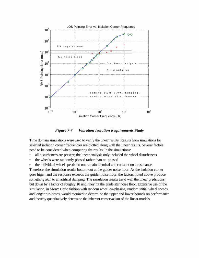
Figure 7-7 Vibration Isolation Requirements Study

Time domain simulations were used to verify the linear results. Results from simulations for selected isolation corner frequencies are plotted along with the linear results. Several factors need to be considered when comparing the results. In the simulations: • all disturbances are present; the linear analysis only included the wheel disturbances • the wheels were randomly phased rather than co-phased • the individual wheel speeds do not remain identical and constant on a resonance Therefore, the simulation results bottom out at the guider noise floor. As the isolation corner goes higer, and the response exceeds the guider noise floor, the factors noted above produce something akin to an artifical damping. The simulation results trend with the linear predictions, but down by a factor of roughly 10 until they hit the guide star noise floor. Extensive use of the simulation, in Monte Carlo fashion with random wheel co-phasing, random initial wheel speeds, and longer run-times, would required to determine the upper and lower bounds on performance and thereby quantitatively determine the inherent conservatism of the linear models.

10-2 10-1 100 101 10210-4

10-3

10-2

10-1

100

101

102

103

Isolation Corner Frequency (Hz)

RM

S P

oint

ing

Err

or (m

as)

LOS Pointing Error vs. Isolation Corner Frequency

O - l i n e a r a n a l y s i s

3 - s r e q u i r e m e n t

X - s i m u l a t i o n

G S n o i s e f l o o r

n o m i n a l F E M , 0 . 0 0 1 d a m p i n g ,

n o m i n a l w h e e l d i s t u r b a n c e s

8. Conclusions The integrated models have allowed us to validate the basic design of the NGST Yardstick. The models were exercised to predict the line-of-sight and wavefront errors resulting from three significant loads, or disturbance sources. The predicted performance under all conditions was not acceptable after the first iteration. But use of the models allowed design alternatives to be explored until acceptable performance was achieved. The results of the static analysis presented in section 6 indicate that the changes in shape due to ground-to-orbit bulk cool-down of the telescope structure are within the expected capture range of the baseline wavefront sensor. All other things being equal, we should therefore be able to initially align and phase the segmented primary mirror. Additional contributions to initial segment misalignment, such as latch and hinge tolerances, must also be taken into account. However, the results for a quasi-static analysis of a thermal transient event show that the telescope is not passively stable. The wavefront error allocation is exceeded almost immediately at the start of a large angle slew. In addition, the thermal environment of the OTA is such that days may be required to reach equilibrium following a slew. Either structural re-design for passive stability, or active wavefront control, is therefore required. Both active temperature and active wavefront control using heaters was demonstrated to be feasible. Both are promising alternatives to either the use of a dedicated instrument for wavefront sensing or the interruption of observations to employ the baseline image-based phase-retrieval sensor. Finally, the results given in section 7 for the dynamic analysis indicate that disturbances from the reaction wheels coupled with the lightly-damped and highly-flexible structure present significant challenges to the baseline line-of-sight control architecture. Vibration isolation will be required to meet jitter error requirements. The low-frequency isolation requirements may present a challenge to the current state-of-the-art. In addition, significant uncertainty exists regarding damping in complex, precision structures at cryogenic temperatures. The assumptions made in the analysis regarding damping were considered conservative, but attention must be paid to this issue as NGST evolves.

9. References 1. Bely, P.Y., Perrygo, C. and Burg, R., NGST “Yardstick” Mission, NGST Monograph No. 1,

July 1999 2. Integrated Modeling of Optical Systems User’s Manual, Release 2.0, JPL D-13040,

November 15, 1995 3. Redding, D.C., Levine, B.M, Yu, J.W., and Wallace, J.K., “A Hybrid Ray Trace and

Diffraction Propagation Code for Analysis of Optical Systems,” SPIE Vol. 1625, Design, Modeling, and Control of Laser Beam Optics, 1992

4. Perrygo, C. and Burg, R., “Hand calculation of line-of-sight sensitivity to optics displacements,” NGST Systems Engineering Memo, January 22, 1999

5. Oppenheimer, B.R., Palmer, D., Dekany, R., Sivaramakrishnan, A., Ealey, M. and Price, T., “Investigating a Xinetics Inc. Deformable Mirror,” publication date unavailable

6. Thermal Radiation Analyzer System (TRASYS) User’s Manual, Lockheed Engineering Management Services Company, JSC-22964, October 1991

7. Parrish, K., “Baseline Yardstick Thermal Results after Model Updates and Conversion to TSS,” NGST Systems Engineering Report (THSER03), February 8, 1998

8. Parrish, K., “Updated Thermal Modeling Process using FEMAP, TSS, TCON, and SINDA85,” NGST Systems Engineering Report (THSER02), May 4, 1998

9. Bolz, R. E. and Tuve, G. L., “Handbook of Tables for Applied Engineering Science,” 2nd Edition, CRC Press, Boca Raton, 1976, pp. 528

10. Mosier, G.E., Femiano, M.D., Ha, K.Q., Bely, P.Y., Burg, R., Redding, D.C., Kissil, A., Rakoczy, J. and Craig, L., “Fine Pointing Control for a Next Generation Space Telescope,” SPIE Vol. 3356, Space Telescopes and Instruments V, 1998

11. Murrell, J.W., “Precision Attitude Determination for Multimission Spacecraft,” AIAA, 1978 12. Bauer, F.H., Femiano, M.D., and Mosier, G.E., “Attitude Control System Conceptual Design

for the X-ray Timing Explorer,” AIAA, 1992 13. Farrenkopf, R.L., “Analytic Steady-State Accuracy Solutions for Two Common Spacecraft

Attitude Estimators,” Journal of Guidance and Control, Vol. 1, No. 4, July-August 1978 14. Bialke, B., “Microvibration Disturbance Sources in Reaction Wheels and Momentum

Wheels,” Proc. Conference on Spacecraft Structures, Materials & Mechanical Testing, Noordwijk, The Netherlands, March 27-29, 1996

15. Melody, J.W., “Discrete-Frequency and Broadband Reaction Wheel Disturbance Models,” Jet Propulsion Laboratory Interoffice Memorandum 3411-95-200csi, June 1, 1995

16. Spanos, J., Rahman, Z., and Blackwood, G., “A Soft 6-axis Active Vibration Isolator,” American Control Conference, Seattle, June 21-23, 1995

17. Spanos, J. and Rahman, Z., “Control Concepts for Active Multi-axis Vibration Isolation,” Proc. 6th Intl. Conf. On Adaptive Structures, Key West, Florida, Nov. 13-15, 1995

18. Germann, L. and Lawrence, D., Left Hand Design Corp. white paper for NGST feasibility study, July 1996

19. Paplexandris, M. and Redding, D.C., “Active Thermal Control of Wavefront Error of NGST,” JPL Interoffice Memorandum, May 20, 1999

Documents

NGST Monograph No. 6 Performance Analysis Using Integrated Modeling · 2015-07-02 · NGST Monograph No. 6 Performance Analysis Using Integrated Modeling By Gary Mosier, Keith Parrish,