Learning by Doing, Export Subsidies, and Industry Growth:

Japanese Steel in the 1950s and 1960s

Hiroshi Ohashi ∗

December 2003

Abstract

The paper examines the Japanese steel industry in the 1950s and 1960s to evaluate

the role of export subsidy policies. Export subsidies can be instrumental in increasing

an industry’s cost competitiveness in the presence of learning by doing, a characteristic

of production in the steel industry. The proposed approach addresses identification

issues found in the literature. Using a dynamic estimation model, this paper identifies

a significant learning rate of above 20%. It also finds little intra-industry knowledge

spillover, an observation consistent with the nature of the Japanese employment system

at that time. Simulations made with the model indicate that the subsidy policy had

an insignificant impact on industry growth. The paper provides underlying economic

reasons for the simulation results.

Key words: Learning by doing, export subsidies, knowledge spillover, industry growth.

JEL: D21; F13; L61; O12

∗I am grateful to Tsuyoshi Nakamura who generously provided me with the data set and patiently answered my

questions on the Japanese steel industry. I thank Kenzo Abe, James Adams, Elias Dinopoulos, Elhanan Helpman,

Tsuyoshi Nakamura, Ariel Pakes, Nina Pavcnik, John Ries, Jeffrey Williamson, three anonymous referees, and par-

ticipants at several seminars and conferences for their useful comments. Correspondence: Faculty of Commerce,

University of British Columbia; Faculty of Economics. University of Tokyo. 7-3-1 Hongo, Tokyo, Japan, 133. Phone:

+81-3-5841-5511. E-mail: ohashi@e.u-tokyo.ac.jp

1

1 Introduction

The East Asia region has been the envy of developing countries for most of the postwar period.

Striking economic growth helped rapidly push the region up the development ladder to join the

elite group of high-income countries. Many economists have speculated as to the reasons for this

East Asian miracle. The superior accumulation of physical and human capital has been considered

by many to be an important factor contributing to their success. However, considerable debate still

exists as to whether export-promoting policies, which many Asian countries implemented, were an-

other key driving force behind the Asian miracle. Some researchers judge that governments shaped

the course of development (for example, Sachs and Warner, 1995), whereas others discount the role

of government trade policies in the development process (for example, Patrick and Rosovsky, 1976;

Rodríguez and Rodrik, 2000). Understanding the extent to which policy instruments contributed

to rapid growth in East Asia is essential for other developing countries attempting to get their

policy fundamentals right.

Many cross-country studies have investigated the relationship between trade policies and eco-

nomic growth (see Baldwin, 2003, for a recent survey). There is, however, a major identification

problem in separating the effects of outward-orientated trade policies and sensible macroeconomic

policies in the analysis (argued in Rodríguez and Rodrik, 2000; Srinivasan and Bhagwati, 2001).

Outward-oriented economies have often implemented macroeconomic stabilization programs, such

as setting realistic exchange rates and maintaining moderate fiscal deficits. The lack of observable

controls makes it difficult to distinguish the effects of trade policies from those of macro policies.

Furthermore, after taking account of the diversity of countries and the various forms of trade policies

implemented by them, it is difficult to serve a consistent cross-country relationship between trade

policies and economic growth: there may not be enough cross-country variation fully to control for

such heterogeneity.1

In explaining their reasons for being unable to provide a rigorous policy analysis, the World

Bank (1993) discusses an alternative methodology to avoid the identification problem that haunts

the literature:

[I]t is very difficult to establish statistical links between growth and a specific interven-

tion, even more difficult to establish causality. Because we cannot know what would1Similar criticisms apply to the literature of within-country cross-industry studies, as discussed in Section 6.

2

have happened in the absence of a specific policy, it is difficult to test whether inter-

ventions increased growth rates. [W]e cannot offer a rigorous counterfactual scenario.

(p6)

Stiglitz (2001) recently made a similar point in concluding the volume entitled Rethinking the

East Asian Miracle:

[T]he problem of interpreting the [Asian] miracle, crisis, and recovery is that we have

an underidentified system: we do not have the controlled experiments that would allow

us to assess what would have happened. (p522)

The paper presents an estimation framework that conducts such counterfactual exercises to

assess the role of trade policy in growth. Although there seems no obvious opportunity to conduct

controlled experiments on trade policy, we can still perform counterfactual exercises by following

two steps: first use observed data along with an economic model to recover estimated parameters

of underlying economic primitives that are invariant to policy environment. In this application,

I estimate the parameters of firm cost functions. The second step involves using the model to

simulate changes in equilibrium outcomes resulting from changes in the underlying trade policy

(export subsidy in this case). For this simulation approach to be successful, the model used for the

exercise must closely approximate the economic environment under study, and the trade policy of

interest must be exogenous to the environment. To my knowledge, this is the first study using the

framework suggested above to evaluate the effectiveness of outward-oriented policy in contributing

to the Asian miracle.

More specifically, this paper focuses on the Japanese steel industry in the 1950s and 1960s. The

Japanese steel industry is an ideal case for examining the effects of export subsidies: after World

War II, the steel industry experienced unprecedented growth in production, climbing from less than

a fraction of 1 percent of the world market in 1946 to 17 percent in 1973. The industry was also the

object of a highly visible export subsidy policy, in place from 1955 to 1964. This paper analyzes

the extent to which this export policy may have accounted for steel industry growth. This is a first

step in investigating whether government export interventions contribute to economic growth in

general, and future studies will measure the effects of inter-industry externalities on such growth.

The Japanese steel industry experienced dramatic changes after the devastation of the Second

World War, when more than 70 percent of blast furnaces were out of operation due to the aftermath

3

of bombardment and the lack of foreign exchange for raw material purchase. Shortly after the war,

the government designated steel as a priority sector. The most conspicuous policy in the 1950s and

1960s was the implementation of an export subsidy, which came into effect in 1953. The subsidy

rate was originally set at 3 percent of a firm’s export revenue. After occasional revisions, the

subsidy was eventually phased out in 1965 (see Figure 1). The same subsidy system was applied to

all Japanese exporting sectors during the period, and appeared to be instated independent of the

interests of the steel industry. Interestingly, however, the period of subsidy provision coincides with

a period of remarkable growth in the industry, and the steel industry expanded production more

than fourfold between 1953 and 1964. This not only met rapidly growing domestic demand but

also stimulated steel exports, which grew at over 20 percent annually, raising Japan to the status

of the world’s largest steel exporter in 1969.

Industry circles have recognized that producing steel involves substantial learning in production.

Given experience of repetitive tasks, steel workers are likely to learn from cumulative experience how

such tasks can be done more quickly and efficiently. If such “learning by doing” is indeed integral

to steel production, the export subsidy, even though it was only 4.5 percent at its highest, could in

principle have made a large difference to the evolution of the Japanese steel industry. The question

is how important this effect was. The paper estimates the magnitudes of the effect of learning

by doing and inter-firm knowledge spillover on growth within the industry. These estimates are

based on a dynamic model of production technology that incorporates the importance of learning

by doing. The paper then runs the model to analyze the impact of the export subsidy using the

obtained estimates.

This paper contributes to both the literature on the evaluation of trade policy, and the liter-

ature on the estimation of learning by doing. Irwin and Pavcnik (2001) examine recent aspects

of the Airbus-Boeing rivalry to study the effects of subsidy, the policy implications of which were

first studied by Brander and Spencer (1985). Their study lacks, however, any analysis of learning

in the aircraft industry. Though the international steel market appeared to have been perfectly

competitive during my study period, the export subsidy must have usefully helped boost cost com-

petitiveness because of the concurrent presence of learning by doing. A handful of case studies have

evaluated the performance of tariff protection policies in the presence of learning by doing. These

papers either use calibration (Baldwin and Krugman, 1988; Miravete, 1998), or static estimation

with the assumption of complete knowledge spillovers (Head, 1994). It is well known that the

4

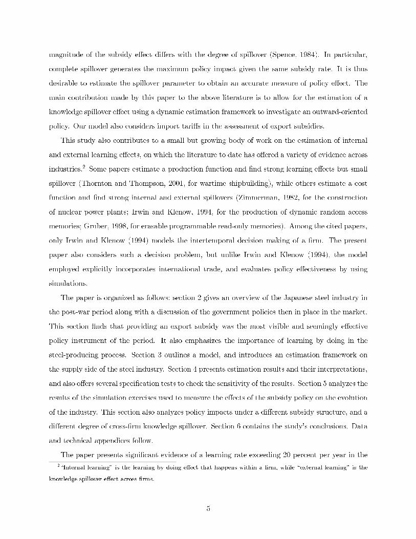
magnitude of the subsidy effect differs with the degree of spillover (Spence, 1984). In particular,

complete spillover generates the maximum policy impact given the same subsidy rate. It is thus

desirable to estimate the spillover parameter to obtain an accurate measure of policy effect. The

main contribution made by this paper to the above literature is to allow for the estimation of a

knowledge spillover effect using a dynamic estimation framework to investigate an outward-oriented

policy. Our model also considers import tariffs in the assessment of export subsidies.

This study also contributes to a small but growing body of work on the estimation of internal

and external learning effects, on which the literature to date has offered a variety of evidence across

industries.2 Some papers estimate a production function and find strong learning effects but small

spillover (Thornton and Thompson, 2001, for wartime shipbuilding), while others estimate a cost

function and find strong internal and external spillovers (Zimmerman, 1982, for the construction

of nuclear power plants; Irwin and Klenow, 1994, for the production of dynamic random access

memories; Gruber, 1998, for erasable programmable read-only memories). Among the cited papers,

only Irwin and Klenow (1994) models the intertemporal decision making of a firm. The present

paper also considers such a decision problem, but unlike Irwin and Klenow (1994), the model

employed explicitly incorporates international trade, and evaluates policy effectiveness by using

simulations.

The paper is organized as follows: section 2 gives an overview of the Japanese steel industry in

the post-war period along with a discussion of the government policies then in place in the market.

This section finds that providing an export subsidy was the most visible and seemingly effective

policy instrument of the period. It also emphasizes the importance of learning by doing in the

steel-producing process. Section 3 outlines a model, and introduces an estimation framework on

the supply side of the steel industry. Section 4 presents estimation results and their interpretations,

and also offers several specification tests to check the sensitivity of the results. Section 5 analyzes the

results of the simulation exercises used to measure the effects of the subsidy policy on the evolution

of the industry. This section also analyzes policy impacts under a different subsidy structure, and a

different degree of cross-firm knowledge spillover. Section 6 contains the study’s conclusions. Data

and technical appendices follow.

The paper presents significant evidence of a learning rate exceeding 20 percent per year in the2“Internal learning” is the learning by doing effect that happens within a firm, while “external learning” is the

knowledge spillover effect across firms.

5

Japanese steel industry in 1955-1965. It finds only a small intra-industry spillover effect, which may

reflect the nature of the Japanese labor market at that time. The simulation exercises demonstrate

that the subsidy provided by the government until 1964 contributed only minimally, accounting

for an average of just 2 percent of the output increase in 1955-1968. The effect of the subsidy

would have been much larger if firms had shared their experience with one another: a subsidy can

alleviate the free rider problem. The paper finds that the impact of the subsidy policy critically

depends on the slope of a dynamic supply curve.

2 An Overview of the Japanese Steel Market

Japan’s miraculous growth from the 1950s through the 1970s has been closely studied by economists

and policy makers. Japan’s experience has been taken as a prototype of the so-called “flying goose

model” in which industries experience rapid growth one after another, with a lead industry providing

external benefits to subsequent industries that help them take off. In this context, the steel industry

was the “lead goose” in Japan’s marvelous growth after the Second World War, followed by the

TV and automobile industries.

This section provides an historical overview of the Japanese steel market. Beginning with

a description of government policies affecting the steel industry during the post-war period, the

section goes on to explain some unique aspects of steel production in Japan. “Learning by doing”

appears to be important in steel production. The nature of human capital accumulation along with

the unique labor market practices in Japan may, however, have prevented steel firms from sharing

their experience with one another.

2.1 Government Interventions in the Post-war Era

The Japanese steel industry faced many challenges in the early post-war era. The industry had lost

its traditional sources of raw materials in Northeastern Asia (Manchuria), and did not have enough

foreign exchange to purchase raw materials elsewhere. As a consequence, 70 percent of the blast

furnaces in Japan ceased operations in 1946. Steel production dropped to just over 0.5 million tons

in 1946 from a wartime peak of 7.5 million tons just three years earlier.

The Japanese government decided to implement policies to revive the steel industry as quickly

6

as possible.3 The first policy was a rationalization program. It involved concessional loans to the

industry and rearrangements of payment schedules for previous government loans. The government

also gave steel firms preferential tax treatment, including lower property taxes and accelerated

depreciation rates. Foreign exchange loans were provided to help their purchase of raw materials.

As a result, by 1955 steel production was restored to its war time peak (see Figure 1). At this

point, all government interventions were essentially replaced by import tariffs and export subsidies.

Japan had an import tariff of 15 percent on steel until 1967 when it agreed to drop the rate

to 12 percent at the Kennedy Round of GATT. Until that point, the tariff system had remained

unaltered since its inception, with the exception of six months in 1957 (April - October) when the

tariff was temporarily interrupted in response to a surge in demand that accompanied an economic

boom. While the import tariff doubtless protected domestic steel makers from direct competition

with foreign steels, it may have had little to do with the increase in Japanese steel production shown

in Figure 1, because of the fact that Japan also exported steels during the period. We discuss how

the import tariff comes into play in our estimation model in Section 3.1.

The most visible government policy that seems to have had great impact on the industry in

the 1950s and 1960s was the export subsidy provided by the Ministry of International Trade and

Industry (MITI). The trade journal published by Japan Iron and Steel Federation (1969) also

acknowledged that the policy had greatly benefitted the industry. The marginal rate of subsidy on

the average firm is illustrated in Figure 1.4 The subsidy came into effect in 1953 and was based

on a firm’s annual export revenue, the rate being originally set at 3 percent. In April 1957, the

government amended the policy to provide a 4.5 percent subsidy on export revenues exceeding

half the revenue of the previous year. This amendment was terminated in 1961, and the subsidy

itself was phased out as Japan became a member of GATT. The subsidy system was applied to all

exporting sectors including two major industries: textiles and machinery. Textiles were the largest

export when the subsidy system was introduced. Textile exports, however, dropped considerably

in the period, declining from 30 percent of total Japanese exports in 1955 to 15 percent in 1963.

Machinery exports, on the other hand, started taking off in the late 1960s. The coverage of various

exporting sectors should have made it difficult for MITI to lobby in favor of any particular industry3See Yamamura (1986) for a general survey of Japanese industrial policies.4The Japanese subsidy system had two tracks, one based on export revenue and the other on export profit. Each

company was assigned to a track that would cost the government the least. The subsidy of the steel industry was

based on export revenue during the period considered here (Japan Iron and Steel Exporters’ Association, 1974).

7

in establishing a uniform export subsidy across all sectors.5 Our simulation exercises exploit this

aspect of the subsidy policy, namely, the fact that the policy appeared exogenous to the promotion

of the steel industry.

Interestingly, the period of the subsidy provision coincides with a time of remarkable growth

in the industry. Japanese steel production quadrupled from 1953 to 1964. This rapid production

growth was accompanied by export expansion, and Japan’s share of the world export market grew

from under 5 percent in 1955 to 9 percent in 1965. Most of Japan’s steel had been shipped to Asian

countries until the early 1960s, when an increasing proportion began to go to North America. The

steel export market was fairly competitive from 1955 to 1965, and there is little evidence that

Japanese steel makers played a significant role in the world steel market during the period. Japan

Iron and Steel Exporters’ Association (1974) observed that the Japanese FOB steel price was not

significantly different from the price in Antwerp, Belgium, the center of the world steel trade at

that time.6

We chose to study the steel industry over other sectors, because Japanese steel in the post-war

period has often been described as a great success story attributable to government interventions.

We have focused on the export subsidy over other policy interventions because the policy was likely

exogenous to the promotion of the industry. It is this aspect of the policy that helps us identify

the impact it had on the industry’s growth. Of course, one could analyze the policy’s impact on

another export sector, say, the cotton industry. It may well have been that this industry declined

much more slowly with the subsidy provision.5Along with MITI’s export subsidies, the Bank of Japan also provided interest-rate subsidies on export credit.

Once a firm had an export order, it needed credit to finance the production and sale until it received payment from

the buyer. The bank offered such credit with interest at below market rates (the difference in the rates was in the

range of 2-3 percent). The total amount of this subsidy was, however, limited and application was therefore restricted

to only a few large export orders. The export-credit subsidy was therefore likely to have had only a marginal impact

on steel exports (Miwa and Ramseyer, 2001). The paper thus does not focus on this export credit subsidy.6One could argue that export subsidies might have been prone to abuse, because the export goods were in general

less likely to receive thorough inspection (See Panagariya, forthcoming). It is hard to argue against the possibility of

the over-invoicing of exports given poor documentation of the actual administrative procedure for MITI’s granting

the subsidies at that time. However, I believe that this moral hazard would not have been significant, based on

comparison of figures from two different sources. The difference between domestic steel production and shipments,

net of inventory, reveals (according to data published by MITI) that, on average, 12.8% of domestic steel should have

been exported from 1955 to 1968, a figure consistent with evidence reported in trade data (published by the Ministry

of Finance).

8

2.2 Learning in Steel Production

Over 70 percent of Japanese steel production in the 1950s and 1960s was accounted for by integrated

steel manufacturers.7 Six integrated steel companies controlled the major share of the market:

Yawata, Fuji, Nihon Kokan, Kawasaki, Sumitomo, and Kobe (in order of average market share).

My analysis thus focuses on these six firms.8

Integrated steelworks transform raw materials (iron ore and coking coal) into pig iron in a blast

furnace. Pig iron is then transformed into crude steel in a second furnace by removing carbon

and other elements. The prevalent technology used throughout most of our study period in this

second stage was the open-hearth furnace (referred to as OH), which blows air from the bottom

of a brick-lined steel shell through the molten pig iron. The air raises the temperature in the pig

iron and oxidizes the carbon in it. A basic oxygen furnace (referred to as BOF) was introduced in

Japan in the late 1950s and progressively replaced the OH. Though the presence of the OH was

significant in Japan’s steel industry, the use of the BOF was increasingly popular to the point that

the share of BOF in the total steel production was over 50 percent in 1965, up from only 12 percent

in 1960 (see Lynn, 1982, for a description of the BOF adoption process in Japan).

Steel production could not be performed without skilled workers. An integral part of production

is temperature control in the blast furnace (see Itami, 1997, for details). Furnace temperature

control is now fully computerized, but in the 1950s it had to be done manually. To produce steel of

sufficient durability with efficient energy consumption, the furnace temperature has to be adjusted

according to the qualities of the raw materials and the specific conditions of the fabrication process.

For instance, for efficient steel production, the optimal furnace temperature should be higher when

there is humidity in a furnace and lower when the quality of iron ore is higher. When adjustments

were made manually, the frequency and size of the adjustments were determined by the experience

and judgment of the steelworkers. Many attempts had been made to standardize the temperature

control process by using statistical techniques, but these failed because the yields depended on

so many conditions specific to a plant (Japan Iron and Steel Association, 1965). Accumulated

knowledge and experience embodied in skilled workers hence appeared to play an important role7The other steel-making process, electric steel production, was generally used to make stainless or other special

steels, and is not discussed here. Use of this technology has become widespread only recently, with the development

of mini-mills in which manufacturers use a combination of an electric arc furnace and continuous casting technology.8We discuss an issue of the sample selection in Section 3.1.

9

in an efficient steel-production operation.9

The characteristics of steel production mentioned above suggest that experience gained in one

firm was not necessarily transferable to other firms because it was fairly specific to individual

plants. Another obstacle to sharing experience among firms was the unique Japanese job practices

of seniority and lifetime employment. These were vigorously adopted by Japanese industries across

the board shortly after World War II in order to secure the work force. Since experience was often

embodied in workers, these practices, by preventing the turnover and layoff of skilled workers, would

have substantially reduced the flow of experience among firms.

3 The Model and Estimation Methods

3.1 Overview of the Model

This section describes a model used to explain the Japanese steel market in 1955-1965. I begin the

section by providing an overview of the estimation model used in the paper, details of which are

described in the remainder of this section.

The estimation model considers Japan as a small country, which exports and imports in a com-

petitive world steel market: the Japanese export share of the world market was only 9 percent

at its highest, and its import share accounted for a mere 0.3 percent of world production even

without tariffs. A wide variety of industries consume steel as an intermediate input, ranging from

automobile production to construction and shipbuilding. It is likely that domestic and imported

steels were perceived as imperfect substitutes for each other, since their prices were substantially

different. Section 4 reports that the standard error of the import price is four times that of domes-

tically produced steel, and with a higher mean. The feature of product differentiation generates

a downward-sloped domestic demand: demand for domestic steel decreases with price, as some of

the demand is satisfied instead by imported steel (see Appendix B for further discussion).9The industry trade association appeared to recognize the existence of learning by doing in steel production. Japan

Iron and Steel Federation (1970b: hereafter JISF) documents the changes in the inputs of coking coal and labor hours

from 1955-1969. The consumption of coking coal per ton of steel production decreased from 700kg to 500kg, while

labor inputs dropped from 8 hours to just over 1 hour by the end of the period, a drastic efficiency improvement

of over 80%. Though JISF (1970b) associates the efficiency improvement with learning by doing, there must have

been other factors (such as technological innovations) that accounted for the increase in productivity. Section 3.2

incorporates such factors in order to identify learning effects.

10

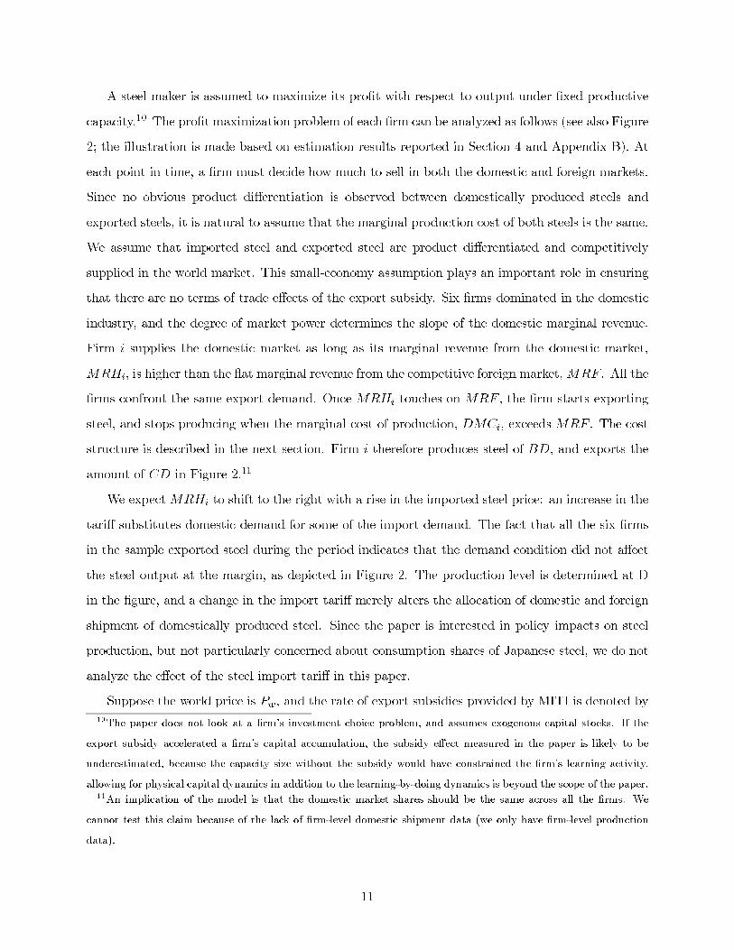
A steel maker is assumed to maximize its profit with respect to output under fixed productive

capacity.10 The profit maximization problem of each firm can be analyzed as follows (see also Figure

2; the illustration is made based on estimation results reported in Section 4 and Appendix B). At

each point in time, a firm must decide how much to sell in both the domestic and foreign markets.

Since no obvious product differentiation is observed between domestically produced steels and

exported steels, it is natural to assume that the marginal production cost of both steels is the same.

We assume that imported steel and exported steel are product differentiated and competitively

supplied in the world market. This small-economy assumption plays an important role in ensuring

that there are no terms of trade effects of the export subsidy. Six firms dominated in the domestic

industry, and the degree of market power determines the slope of the domestic marginal revenue.

Firm i supplies the domestic market as long as its marginal revenue from the domestic market,

MRHi, is higher than the flat marginal revenue from the competitive foreign market,MRF . All the

firms confront the same export demand. Once MRHi touches on MRF , the firm starts exporting

steel, and stops producing when the marginal cost of production, DMCi, exceeds MRF . The cost

structure is described in the next section. Firm i therefore produces steel of BD, and exports the

amount of CD in Figure 2.11

We expectMRHi to shift to the right with a rise in the imported steel price: an increase in the

tariff substitutes domestic demand for some of the import demand. The fact that all the six firms

in the sample exported steel during the period indicates that the demand condition did not affect

the steel output at the margin, as depicted in Figure 2. The production level is determined at D

in the figure, and a change in the import tariff merely alters the allocation of domestic and foreign

shipment of domestically produced steel. Since the paper is interested in policy impacts on steel

production, but not particularly concerned about consumption shares of Japanese steel, we do not

analyze the effect of the steel import tariff in this paper.

Suppose the world price is Pw, and the rate of export subsidies provided by MITI is denoted by10The paper does not look at a firm’s investment choice problem, and assumes exogenous capital stocks. If the

export subsidy accelerated a firm’s capital accumulation, the subsidy effect measured in the paper is likely to be

underestimated, because the capacity size without the subsidy would have constrained the firm’s learning activity.

allowing for physical capital dynamics in addition to the learning-by-doing dynamics is beyond the scope of the paper.11An implication of the model is that the domestic market shares should be the same across all the firms. We

cannot test this claim because of the lack of firm-level domestic shipment data (we only have firm-level production

data).

11

s. The competitive foreign market makes MRF equal to Pw · (1 + s). If the elimination of export

subsidies (i.e., s = 0) shifts the foreign marginal revenue curve toMRF∗ in Figure 2, firm i reduces

its exports from CD to EF . IfMRF∗ lies below G, however, firm i would stop exporting. It is thus

necessary to check whether each firm would still have had an incentive to export in the absence of

the subsidies. This analysis requires the estimation ofMRHi derived from estimated domestic steel

demand (see Appendix B for this analysis). To anticipate the result, I found that all the firms would

have chosen to export even without the provision of the subsidies.12 For the simulation exercises

to work, s needs to be exogenous. Since the same rate was applied to all exporting sectors across

the board in Japan, MITI would not be able to lobby in favor of the steel industry. Although

it is difficult to determine just how the rate was established in the policy-making process, it is

reasonable to think of the subsidy rate as exogenous to the steel makers.

As mentioned above, in the 1950s and 1960s, the six integrated steel companies that controlled

over 70 percent of the domestic market form the basis of my analysis. All the firms remained in the

market throughout my study period, and thus we do not consider the issue of firm entry and exit.

Since most learning by doing activities must have occurred in large firms, this sample selection

might have led to overstating the effects of the subsidy. Section 5 reports that the effect of the

export subsidy is small even without regard for this sample selection.

While the paper is concerned with the effects of the export subsidy on industry growth, it would

be useful to discuss the welfare implication of the policy. In a perfectly competitive market with

no externalities, the traditional argument is against an export subsidy; in a small open economy,

no type of trade intervention can be first best, and in a large economy, the exports should be taxed

rather than subsidized to improve the terms of trade. Subsidies to some exports may yet to be

desirable if, as a result, the terms of trade of other exports are improved (Feenstra, 1986; Itoh and

Kiyono, 1987). This is not the case with steel, however, because the subsidy was applied to all

export sectors at the same rate. In imperfect competitive markets, an export subsidy is sometimes

optimal because it raises the profits of the home firm at the expense of the foreign (Brander and

Spencer, 1985). This result is, however, sensitive to assumptions as to market structure. In our

study of the steel industry subject to a competitive world environment, the export subsidy does not

have a solid rationale; even if learning by doing has externalities, a production subsidy dominates12To save space, we do not discuss theoretical implications of firm i’s not exporting, since this situation does not

occur in the simulations.

12

from the welfare point of view. While it would be interesting to analyze the deadweight welfare

loss by use of the export subsidy, rather than an optimal production subsidy, I defer this welfare

question to future research, and only focus on the effect on industry growth in this paper.

The remainder of Section 3 is organized as follows. I first model steel-production technology.

The description of the industry in the previous section reveals that learning by doing was probably

an important feature of steel production at the time. The model hence incorporates this feature,

as well as other control variables such as input prices, capacity utilization, and physical capital.

I then turn to the supply side to derive an equilibrium relationship. Particular attention is paid

to the inter-temporal decision making of firms through their own production experience. A firm’s

production decision today affects its profitability both now and in the future through its newly

acquired experience. The supply model is estimated in the subsequent section.

3.2 Steel-production Technology

This subsection presents a model of steel-production technology. Availability of firm-level factor

input data is limited, and so I have built a cost function incorporating four important elements of

the steel-production process: learning by doing, capacity utilization, physical capital, and material

inputs. The model allows for knowledge spillovers among steel firms. The unit of analysis is

the firm, and data are of a monthly frequency. The absence of plant-level observations in the data

prevents me from testing the existence of spillover effects across plants within a single firm. Sources

and characteristics of the data set are explained in Appendix A.

Learning by doing is inherently difficult to measure because it is unobservable. Following the

treatment in the literature, I have used a cumulative output level, z, as a proxy for the firm’s learning

level. It is possible that the benefit of learning is transferable across firms. I have borrowed from

Spence (1984) and Dasgupta and Stiglitz (1988), and model the spillover process as

zi,t = θ · zIND,t + (1− θ) · zFi,t.

This process indicates that firm i’s experience, zi, is the weighted average of the industry’s

experience, zIND, and firm i’s own experience, zFi. If the spillover parameter, θ, is estimated

to be zero, the experience is fully appropriated within each firm and firm i’s knowledge is not

communicable to the other firms. The spillover parameter equals one in the case of complete

13

spillover. Experience in that case is fully shared by all the firms in the industry.13 Each company

accumulates its experience only by producing steel. The transition of experience by month is thus

described by zFi,t = zFi,t−1+ qi,t−1, in which qi,t−1 is firm i’s steel output at time t− 1. The initial

value of experience, zFi,0, is set to be one. In the estimation, I extended this model to allow for

knowledge depreciation to check the sensitivity of results.

This analysis does not explore the scope of international spillovers. In the 1950s and 1960s, the

U.S. occasionally sent engineers to provide technical assistance to Japanese steel makers; foreign

publications on state-of-the-art steel-production technologies were also made available in Japan.

Although it is unclear that this window onto foreign knowledge helped Japanese steel makers

increase production efficiency, in large part because experience was fairly firm-specific, our estimate

of learning by doing could possibly be overstated as a result of this assumption.

Also important in production costs is the degree of capacity utilization of steel-production

furnaces. The utilization rate, U , is a productivity measure defined as the current output divided

by the physically available productive capacity of the furnace. It is not obvious how the utilization

rate affects steel-production costs. For low utilization rates, an increase in the rate would decrease

the production cost. However, since capital is fixed at any given time, at high utilization rates

diminishing returns to scale must begin to take place.

The output growth from 1955 to 65 shown in Figure 1 indicates a substantial expansion of

furnace facilities. In fact, the industry’s blast furnace capacity increased roughly at the same rate

as the steel output. The physical capacity, K, was likely to influence the cost of steel production.

Furthermore, considerable variation is observed in the rate of new capacity expansion from one firm

to another: Yawata, the largest steel maker, expanded to five times its original size by installing

more than 8 million tons of new production capacity during the ten-year period. Kobe, the smallest,

added 2 million tons to increase its capacity seven fold. Since new facilities likely embodied the

latest steel-making technology, the differing pace of capacity expansion implies different rates of

technological improvement among firms. I thus use the age of the blast furnace facility to account

for the capital depreciation in the construction of the capital variable.14 I use a depreciation rate

13While data on the patent citations count could in principle provide another way to measure spillovers, such data

do not exist in Japan, because Japan has not instituted a practice of citing other related patents.14The age variable counts the years elapsed after the blast furnace was installed in each plant by firm. The plant-

level capacity size is used as a weight to create a firm-level index. This variable does not consider renovations. Most

renovations were made for repairs, and not to substituted for installing new facilities.

14

of 5 percent in the estimation. I assume that the total cost for firm i at time t takes the following

form:

TCi,t =

[ct · (zi,t)

ϕ· (Ui,t)

λ· (Ki,t)

φ + ui,t

]· qi,t. (1)

This functional form is useful in that the marginal cost has the most common learning curve

assumption, the constant elasticity version, with an additive error term, u.

It is important to control for input prices when estimating a learning rate. Otherwise the

estimated learning rate would be biased upward with decreasing input prices, even without any

learning actually taking place. The major inputs for integrated steel production were iron ore

and labor. Other essential materials, coking coal and electricity, are not included in the estimation

because both inputs were under strict government regulation and thus their prices did not fluctuate

much during the period. The price of input j, wj , and a constant term are included in a Cobb-

Douglas form, ct, with the weights, γj and γ0, to be estimated, i.e., ct = γ0

∏j (wjt)

γj . All firms

are assumed to face the same input prices. The Greek letters, θ, γ0, γj , ϕ, λ, and φ are the supply

parameters to be estimated in the next section.

Other than the four factors described in (1), important influences on the unit cost include R&D

activity and technological innovation. Such supply shocks are captured by the term, u. I allow

this term to have firm and time-specific components (ν, and respectively) in the estimation:

ui,t = νi+t+εi,t, where ε is an error. This fixed-effect treatment deals with efficiency differences

among firms that do not change over time, and industry-wide supply shocks.

While we already control for firm differences in the speed of innovation in physical capital

stocks, ε might still possibly contain unobserved technological progress. The existence of other

unobservables, such as in-house training programs for skilled workers, or advances of transportation

technologies, reinforces this concern. The endogeneity problem and its correction method are

discussed in the next section.

Since it is difficult to find accurate cost data to directly analyze (1), I estimate price-cost margins

by building a competition model and thereby obtain the cost parameters, as described in the next

section.

15

3.3 Output Choice

This subsection uses the cost model to derive an estimable equilibrium relationship. In particular, I

have constructed a steel makers’ profit maximization problem and solved the first-order condition.

The existence of learning by doing engenders a dynamic decision-making problem. In essence,

today’s decision by a firm influences tomorrow’s cost through a change in the level of accumulated

experience. A firm thus takes into account this inter-temporal link when it makes production

decisions.

It is widely believed that the success of post-war Japan was due in part to the government’s

role in tempering domestic competition through weak antitrust enforcement and legalized cartels.

In the 1950s and 1960s, MITI implemented policies to stabilize the steel price and coordinate

investments among firms in capacity expansion. This evidence itself seems to suggest that the

industry might have been in a government-led cartel. However, recent studies (Miwa, 1996; Porter,

Takeuchi, and Sakakibara, 2000) conclude that these government and industry attempts failed to

influence production or stabilize prices. This was because no penalty was imposed on defecting

firms, and thus most firms did not follow MITI’s guidance; rivalry was therefore intense in the steel

market. Based on this recent finding, we established the following supply side model: suppose that

each steel maker i chooses its output, qi,t, at time t to maximize the following sum of expected

discounted profits:

Et

[∞∑

t=s

βt [(TR(qi,t))− TC(qi,t)]

]. (2)

Let TR and TC be the total revenue and cost, the latter defined as (1). Firms discount future

profits according to a common discount factor, β, with a common information set. The discount

factor is set equal to 0.95.15 Total revenue is the sum of the revenues from exporting and domestic

sales.

In determining the outcome of this model, it is important to consider the appropriate equilibrium

concept. The question is whether firms take other firms’ reactions as given (open-loop strategies),

and whether they take into account the effect of their own actions on others’ subsequent actions

(closed-loop strategies). With my interest in estimating the learning parameter as well as the effect

of spillovers, it is difficult enough to obtain a closed-loop solution of our model, let alone to estimate15Other values of β were tried, and it was found that the objective function is fairly flat in the range 0.94< β ≤0.98.

Estimation is difficult to converge in the range 0.98< β.

16

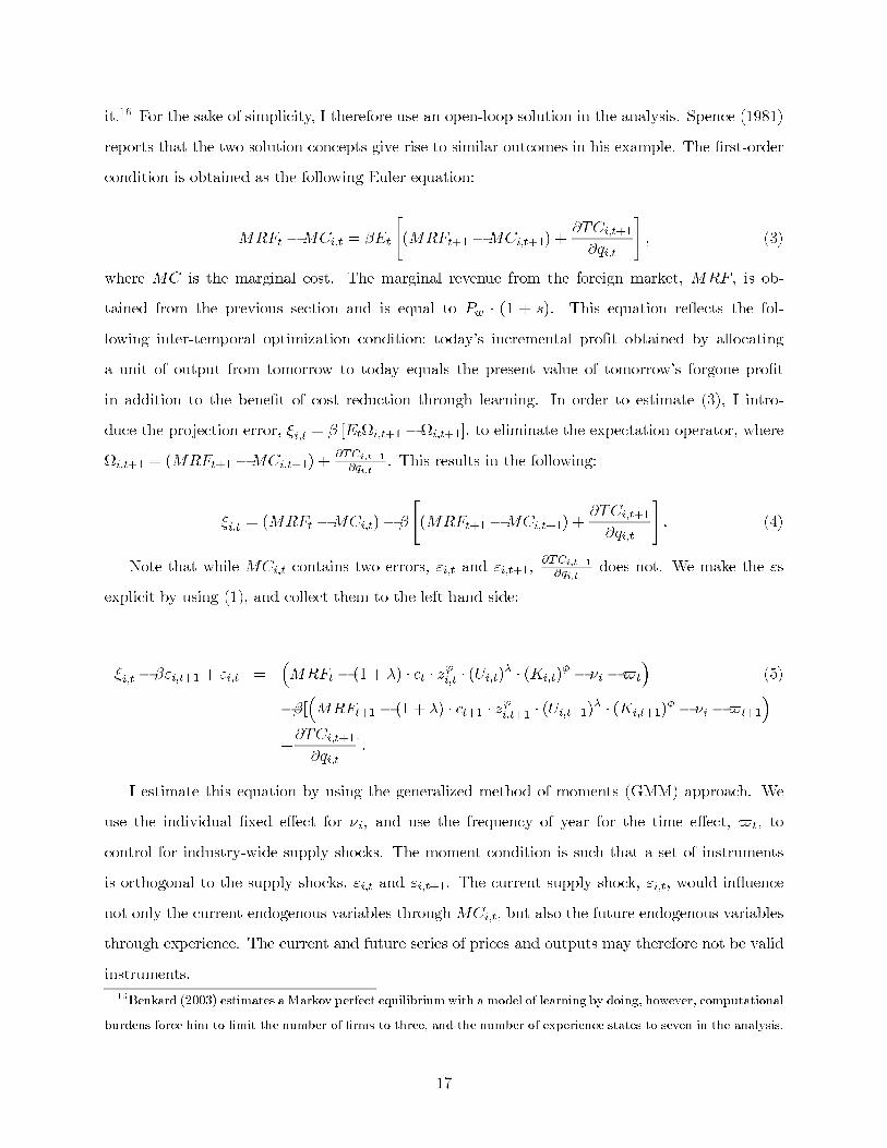
it.16 For the sake of simplicity, I therefore use an open-loop solution in the analysis. Spence (1981)

reports that the two solution concepts give rise to similar outcomes in his example. The first-order

condition is obtained as the following Euler equation:

MRFt −MCi,t = βEt

[(MRFt+1 −MCi,t+1) +

∂TCi,t+1

∂qi,t

], (3)

where MC is the marginal cost. The marginal revenue from the foreign market, MRF , is ob-

tained from the previous section and is equal to Pw · (1 + s). This equation reflects the fol-

lowing inter-temporal optimization condition: today’s incremental profit obtained by allocating

a unit of output from tomorrow to today equals the present value of tomorrow’s forgone profit

in addition to the benefit of cost reduction through learning. In order to estimate (3), I intro-

duce the projection error, ξi,t = β [EtΩi,t+1 −Ωi,t+1], to eliminate the expectation operator, where

Ωi,t+1 = (MRFt+1 −MCi,t+1) +∂TCi,t+1

∂qi,t. This results in the following:

ξi,t = (MRFt −MCi,t)− β

[(MRFt+1 −MCi,t+1) +

∂TCi,t+1

∂qi,t

]. (4)

Note that while MCi,t contains two errors, εi,t and εi,t+1,∂TCi,t+1

∂qi,tdoes not. We make the εs

explicit by using (1), and collect them to the left hand side:

ξi,t − βεi,t+1 + εi,t =(MRFt − (1 + λ) · ct · z

ϕi,t · (Ui,t)

λ· (Ki,t)

φ− νi −t

)(5)

−β[(MRFt+1 − (1 + λ) · ct+1 · z

ϕi,t+1 · (Ui,t+1)

λ· (Ki,t+1)

φ− νi −t+1

)

+∂TCi,t+1

∂qi,t].

I estimate this equation by using the generalized method of moments (GMM) approach. We

use the individual fixed effect for νi, and use the frequency of year for the time effect, t, to

control for industry-wide supply shocks. The moment condition is such that a set of instruments

is orthogonal to the supply shocks, εi,t and εi,t+1. The current supply shock, εi,t, would influence

not only the current endogenous variables throughMCi,t, but also the future endogenous variables

through experience. The current and future series of prices and outputs may therefore not be valid

instruments.16Benkard (2003) estimates a Markov perfect equilibrium with a model of learning by doing, however, computational

burdens force him to limit the number of firms to three, and the number of experience states to seven in the analysis.

17

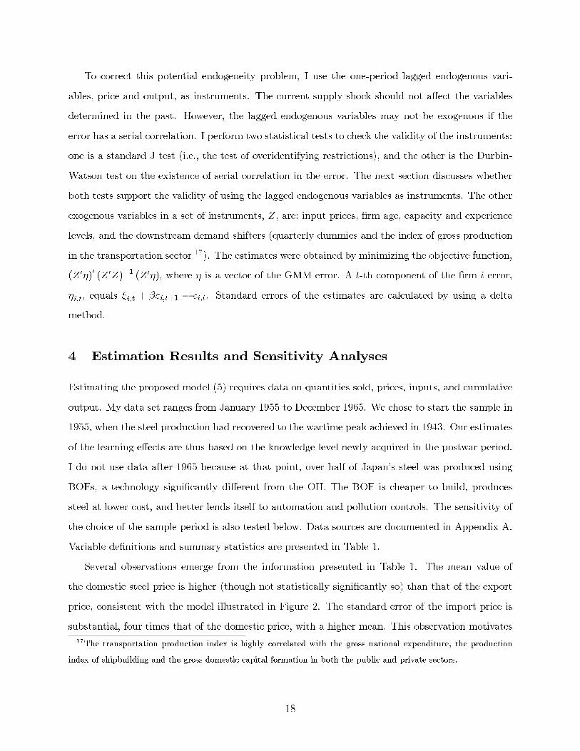
To correct this potential endogeneity problem, I use the one-period lagged endogenous vari-

ables, price and output, as instruments. The current supply shock should not affect the variables

determined in the past. However, the lagged endogenous variables may not be exogenous if the

error has a serial correlation. I perform two statistical tests to check the validity of the instruments:

one is a standard J test (i.e., the test of overidentifying restrictions), and the other is the Durbin-

Watson test on the existence of serial correlation in the error. The next section discusses whether

both tests support the validity of using the lagged endogenous variables as instruments. The other

exogenous variables in a set of instruments, Z , are: input prices, firm age, capacity and experience

levels, and the downstream demand shifters (quarterly dummies and the index of gross production

in the transportation sector 17). The estimates were obtained by minimizing the objective function,

(Z ′η)′ (Z ′Z)−1 (Z ′η), where η is a vector of the GMM error. A t-th component of the firm i error,

ηi,t, equals ξi,t + βεi,t+1 − εi,t. Standard errors of the estimates are calculated by using a delta

method.

4 Estimation Results and Sensitivity Analyses

Estimating the proposed model (5) requires data on quantities sold, prices, inputs, and cumulative

output. My data set ranges from January 1955 to December 1965. We chose to start the sample in

1955, when the steel production had recovered to the wartime peak achieved in 1943. Our estimates

of the learning effects are thus based on the knowledge level newly acquired in the postwar period.

I do not use data after 1965 because at that point, over half of Japan’s steel was produced using

BOFs, a technology significantly different from the OH. The BOF is cheaper to build, produces

steel at lower cost, and better lends itself to automation and pollution controls. The sensitivity of

the choice of the sample period is also tested below. Data sources are documented in Appendix A.

Variable definitions and summary statistics are presented in Table 1.

Several observations emerge from the information presented in Table 1. The mean value of

the domestic steel price is higher (though not statistically significantly so) than that of the export

price, consistent with the model illustrated in Figure 2. The standard error of the import price is

substantial, four times that of the domestic price, with a higher mean. This observation motivates17The transportation production index is highly correlated with the gross national expenditure, the production

index of shipbuilding and the gross domestic capital formation in both the public and private sectors.

18

us to model product differentiation in the demand, as described in Section 3.1.

The capacity utilization rate is high, the average being over 90 percent. This is inconsistent

with the observation that the industry was overwhelmed by the severe capacity expansion race that

dominated the study period (Japan Iron and Steel Federation, 1959). The high utilization rate

revealed by the data is due to the fact that the engineering definition of “capacity” was not meant

to be the maximum available production level. The data on capacity came from companies’ semi-

annual financial reports, which adopted a complicated conversion method endorsed by the Japanese

steel association to calculate capacity. The utilization rate in the data is thus standardized across

firms, but does not reflect the actual level of operational utilization in an economic sense.

The average age of the blast furnace facilities was 17 years, and over half the blast furnaces

in the sample were built after the war (33 of 59 facilities). The ownership of old facilities was

concentrated in the big three firms: Yawata, Fuji, and Nihon Kokan. The oldest blast furnace, first

ignited in 1901, was owned by Yawata. The large variation in the age of furnace facilities leads us

to incorporate capital depreciation into the construction of the physical capital variable. We use a

depreciation rate of 5 percent in the estimation, but the resulting estimate changes little from that

of the no-depreciation case.

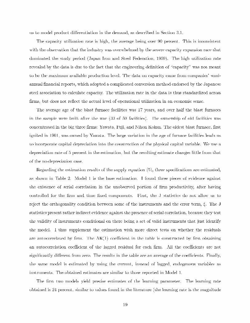
Regarding the estimation results of the supply equation (5), three specifications are estimated,

as shown in Table 2. Model 1 is the base estimation. I found three pieces of evidence against

the existence of serial correlation in the unobserved portion of firm productivity, after having

controlled for the firm and time fixed components. First, the J statistics do not allow us to

reject the orthogonality condition between some of the instruments and the error term, ξ. The J

statistics present rather indirect evidence against the presence of serial correlation, because they test

the validity of instruments conditional on there being a set of valid instruments that just identify

the model. I thus supplement the estimation with more direct tests on whether the residuals

are autocorrelated by firm. The AR(1) coefficient in the table is constructed by first obtaining

an autocorrelation coefficient of the lagged residual for each firm. All the coefficients are not

significantly different from zero. The results in the table are an average of the coefficients. Finally,

the same model is estimated by using the current, instead of lagged, endogenous variables as

instruments. The obtained estimates are similar to those reported in Model 1.

The first two models yield precise estimates of the learning parameter. The learning rate

obtained is 24 percent, similar to values found in the literature (the learning rate is the magnitude

19

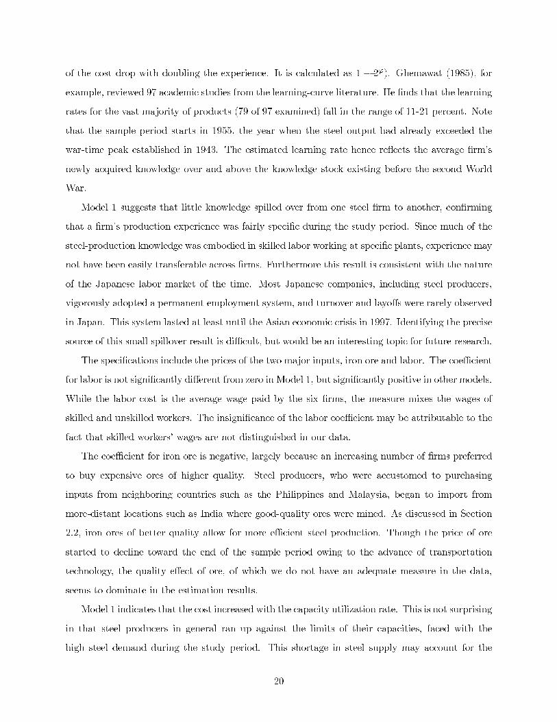
of the cost drop with doubling the experience. It is calculated as 1 − 2ϕ). Ghemawat (1985), for

example, reviewed 97 academic studies from the learning-curve literature. He finds that the learning

rates for the vast majority of products (79 of 97 examined) fall in the range of 11-21 percent. Note

that the sample period starts in 1955, the year when the steel output had already exceeded the

war-time peak established in 1943. The estimated learning rate hence reflects the average firm’s

newly acquired knowledge over and above the knowledge stock existing before the second World

War.

Model 1 suggests that little knowledge spilled over from one steel firm to another, confirming

that a firm’s production experience was fairly specific during the study period. Since much of the

steel-production knowledge was embodied in skilled labor working at specific plants, experience may

not have been easily transferable across firms. Furthermore this result is consistent with the nature

of the Japanese labor market of the time. Most Japanese companies, including steel producers,

vigorously adopted a permanent employment system, and turnover and layoffs were rarely observed

in Japan. This system lasted at least until the Asian economic crisis in 1997. Identifying the precise

source of this small spillover result is difficult, but would be an interesting topic for future research.

The specifications include the prices of the two major inputs, iron ore and labor. The coefficient

for labor is not significantly different from zero in Model 1, but significantly positive in other models.

While the labor cost is the average wage paid by the six firms, the measure mixes the wages of

skilled and unskilled workers. The insignificance of the labor coefficient may be attributable to the

fact that skilled workers’ wages are not distinguished in our data.

The coefficient for iron ore is negative, largely because an increasing number of firms preferred

to buy expensive ores of higher quality. Steel producers, who were accustomed to purchasing

inputs from neighboring countries such as the Philippines and Malaysia, began to import from

more-distant locations such as India where good-quality ores were mined. As discussed in Section

2.2, iron ores of better quality allow for more efficient steel production. Though the price of ore

started to decline toward the end of the sample period owing to the advance of transportation

technology, the quality effect of ore, of which we do not have an adequate measure in the data,

seems to dominate in the estimation results.

Model 1 indicates that the cost increased with the capacity utilization rate. This is not surprising

in that steel producers in general ran up against the limits of their capacities, faced with the

high steel demand during the study period. This shortage in steel supply may account for the

20

positive coefficient on capital. The utilization estimate satisfies the second-order condition to the

maximization problem (2), and generates an upward-sloping supply curve, depicted in Figure 2.

Model 2 concerns with the introduction of the new technology mentioned in Section 2.2. Be-

ginning in 1960, more and more companies switched from the OH to the BOF technology. While

OH still had a significant presence in 1965, there is the possibility that the rate of learning would

have shifted significantly with an increasing number of firms adopting the BOF. In response to this

concern, Model 2 is estimated using a restricted sample period of 1955-60. With the exception of

the greater impacts of labor and physical capital on production cost, the result is similar to that

of Model 1, leading us to believe that the technological switch did not confer a significant impact

on the learning rate at least until the early 1960s.

Finally Model 3 estimates the static learning model, ignoring the future stream of profits in

(4). This assumes that the discount factor is zero. The learning coefficient has an unexpected

sign, and most of the parameters are imprecisely estimated. Though I am not able to reject the

orthogonality hypothesis, the averaged autocorrelation coefficient in firm residuals is significant

at 0.78, and generates a concern for endogeneity. The result of this static model indicates the

importance of firms’ forward-looking behavior due to the existence of learning-by-doing.

The estimated costs of Yawata, the largest steel producer, are depicted in Figure 3. The follow-

ing qualitative features are same for other companies. Annualized average costs (AC), marginal

costs (MC), prices, and dynamic marginal costs (DMC) all appear in the figure, calculated using

the estimates from Model 1. All the data are adjusted by the WPI to constant January 1960

Japanese Yen. The measure, DMCt, is derived from the first-order condition (3) discussed in

Section 3.3:

DMCi,t ≡ MCi,t +

∞∑

s=1

βsEt

[∂TCi,t+s

∂qi,t

]

= MCi,t + βEt

[(MRFt+1 −MCi,t+1) +

∂TCi,t+1

∂qi,t

].

The second equality comes from the Euler equation (4). Both AC and MC were declining

throughout the period because of increasing production experience. The difference between the

marginal and average costs was determined by the utilization coefficient, λ. Since the cost exhibited

decreasing returns (i.e., λ is estimated to be positive), the values of MC were higher than those of

AC. The gap betweenMC and DMC indicates the impact of the firms’ forward-looking behavior:

21

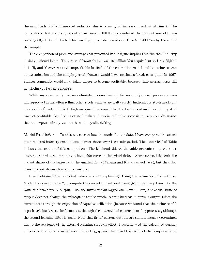
the magnitude of the future cost reduction due to a marginal increase in output at time t. The

figure shows that the marginal output increase of 100,000 tons reduced the discount sum of future

costs by 63,400 Yen in 1955. This learning impact decreased over time to 6,400 Yen by the end of

the sample.

The comparison of price and average cost presented in the figure implies that the steel industry

initially suffered losses. The order of Yawata’s loss was 10 million Yen (equivalent to USD 28,000)

in 1955, and Yawata was still unprofitable in 1965. If the estimation model and its estimates can

be extended beyond the sample period, Yawata would have reached a break-even point in 1967.

Smaller companies would have taken longer to become profitable, because their average costs did

not decline as fast as Yawata’s.

While my revenue figures are definitely underestimated, because major steel producers were

multi-product firms, often selling other steels, such as specialty steels (high-quality steels made out

of crude steel), with relatively high margins, it is known that the business of making ordinary steel

was not profitable. My finding of steel makers’ financial difficulty is consistent with our discussion

that the export subsidy was not based on profit-shifting.

Model Predictions To obtain a sense of how the model fits the data, I have compared the actual

and predicted industry outputs and market shares over the study period. The upper half of Table

3 shows the results of this comparison. The left-hand side of the table presents the predictions

based on Model 1, while the right-hand side presents the actual data. To save space, I list only the

market shares of the largest and the smallest firms (Yawata and Kobe, respectively), but the other

firms’ market shares show similar results.

How I obtained the predicted values is worth explaining. Using the estimates obtained from

Model 1 shown in Table 2, I compute the current output level using (5) for January 1955. For the

value of a firm’s future output, I use the firm’s output lagged one month. Using the actual value of

output does not change the subsequent results much. A unit increase in current output raises the

current cost through the expansion of capacity utilization (because we found that the estimate of λ

is positive), but lowers the future cost through the internal and external learning processes, although

the second learning effect is small. Note that firms’ current outputs are simultaneously determined

due to the existence of the external learning spillover effect. I accumulated the calculated current

outputs to the pools of experience, zF and zIND, and then used the result of the computation in

22

the next period. I repeated the same process for each month until the end of the sample period. I

did not use the estimated supply residual (the estimated value of the left-hand side of (5)), because

otherwise the model will fit the data perfectly.

The results in Table 3 show that the model explains the data well, suggesting that the supply

shock was small. Industry outputs are predicted fairly accurately, if slightly underestimated, while

there is no significant bias in the market share prediction. This provides further evidence that

the supply shock may not contain a strong serial correlation after controlling for the time- and

firm-specific components.

The bottom half of Table 3 presents the out-of-sample predictions. These were made for the

three years (1966-1968) after the period of estimation. Surprisingly, given the change in steel-

production technology during this period, the model explains the data well even in this three-year

period, and especially well in the case of the market shares.

5 Impact of Subsidy Policy

Do government interventions work well in promoting economic growth? The magnitude of the

contribution of trade policy to economic growth remains an open question. This section provides

an answer to the question for the Japanese steel industry. Based on the model and the estimates

reported in the previous sections, this section measures the impact of an export subsidy on industry

growth by asking what would have happened to the steel market had there been no provision of

such government support. Although a small external learning spillover is found in the estimation,

internal learning was identified as a significant source of productivity in steel production. Therefore

the export subsidy, although it was only 4.5 percent at its maximum, could still in principle have

made a large difference in the evolution of the Japanese steel industry. The question is how critical

this effect was.

I conducted the following experiment in determining a firm’s output level, leaving long-run

strategies, such as the level of production capacity, constant. I assumed no subsidy to the steel

industry from 1955 to 1964 (the subsidy was eliminated in 1965, as shown in Figure 1) and calculated

new equilibrium firm outputs for each month. We discussed in Section 3.1 that the subsidy under

study appeared to be exogenous to the promotion of the steel makers, and thus this assumption

should not change the nature of a firm’s cost function estimated in Section 4. The elimination of the

23

subsidy was equivalent to assuming thatMRF equals the world export price, Pw (for which we use

a FOB price). I was concerned with the possibility that some firms would have stopped exporting

in absence of the subsidy. This situation would have occurred in Figure 2 had the no-subsidyMRF

shifted to below G. Appendix B estimates a demand model, and finds that the firms in our sample

would have continued to export even in absence of the subsidy.

I am interested in the output level under the no-subsidy scenario. This is equivalent to finding

the output determined at F in Figure 2 (the intersection between DMCi and MRF ∗). The simu-

lation method used here is similar to the procedure used to predict model fitness in the previous

section. I first replaced all the MRF s in (5) with MRF ∗s (i.e., this is to assume that the subsidy

rate is set at zero). I then used the estimates from Model 1 shown in Table 2 to compute the

current output level using (5) for January 1955. Estimated values were used for the model errors

in the left-hand side of (5). The remaining steps in the simulation method are the same as those

in the method used to calculate the predicted values in the previous section. I ran the model until

the end of 1968, extending the period for three years to see the ensuing impact of the termination

of the subsidy policy.

Figure 4 shows the effect of the subsidy on the industry output level by year. The dotted line

indicates the ratio of the industry output under the subsidy (found in the data) to the simulated

output without subsidy provision. A ratio greater than one indicates that the subsidy had a

positive effect on steel output. A casual inspection of the figure reveals how small the impact was:

the subsidy stimulated a mere 2 percent increase (maximum) in the industry output’s throughout

the period. The output increase is less than 1 percent when the subsidy of 3 percent was in place

at the beginning of the period, and jumps to 1.7 percent in the year when the subsidy rate rose to

4.5 percent. The subsidy had a large effect in 1960 for two reasons. One is that the highest subsidy

rate of 4.5 percent was in place that year. The other is related to the dynamic behavior of firms:

facing a substantial drop in the subsidy of more than one percent in the following year, firms may

have found it more profitable to increase their production levels in 1960 so as to cumulate their

experience. The same economic logic applies to a jump seen in 1963. The impact of the subsidy

tapered off as the subsidy was phased out toward 1965.

It is interesting to observe that actual outputs grew faster than the outputs predicted under

the scenario, even after the actual subsidy system was terminated. This observation is mainly

generated by the relative amount of firms’ experience. The output level without the subsidy does

24

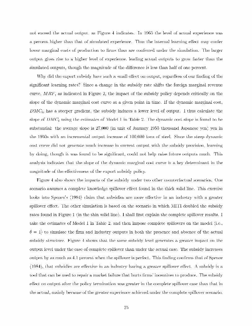
not exceed the actual output, as Figure 4 indicates. In 1965 the level of actual experience was

a percent higher than that of simulated experience. Thus the internal learning effect may confer

lower marginal costs of production to firms than are conferred under the simulation. The larger

output gives rise to a higher level of experience, leading actual outputs to grow faster than the

simulated outputs, though the magnitude of the difference is less than half of one percent.

Why did the export subsidy have such a small effect on output, regardless of our finding of the

significant learning rates? Since a change in the subsidy rate shifts the foreign marginal revenue

curve, MRF , as indicated in Figure 2, the impact of the subsidy policy depends critically on the

slope of the dynamic marginal cost curve at a given point in time. If the dynamic marginal cost,

DMCi, has a steeper gradient, the subsidy induces a lower level of output. I thus calculate the

slope of DMCi using the estimates of Model 1 in Table 2. The dynamic cost slope is found to be

substantial: the average slope is 27,000 (in unit of January 1955 thousand Japanese yen) yen in

the 1950s with an incremental output increase of 100,000 tons of steel. Since the steep dynamic

cost curve did not generate much increase in current output with the subsidy provision, learning

by doing, though it was found to be significant, could not help raise future outputs much. This

analysis indicates that the slope of the dynamic marginal cost curve is a key determinant in the

magnitude of the effectiveness of the export subsidy policy.

Figure 4 also shows the impacts of the subsidy under two other counterfactual scenarios. One

scenario assumes a complete knowledge spillover effect found in the thick solid line. This exercise

looks into Spence’s (1984) claim that subsidies are more effective in an industry with a greater

spillover effect. The other simulation is based on the scenario in which MITI doubled the subsidy

rates found in Figure 1 (in the thin solid line). I shall first explain the complete spillover results. I

take the estimates of Model 1 in Table 2, and then impose complete spillovers on the model (i.e.,

θ = 1) to simulate the firm and industry outputs in both the presence and absence of the actual

subsidy structure. Figure 4 shows that the same subsidy level generates a greater impact on the

output level under the case of complete spillover than under the actual case. The subsidy increases

output by as much as 4.1 percent when the spillover is perfect. This finding confirms that of Spence

(1984), that subsidies are effective in an industry having a greater spillover effect. A subsidy is a

tool that can be used to repair a market failure that hurts firms’ incentives to produce. The subsidy

effect on output after the policy termination was greater in the complete spillover case than that in

the actual, mainly because of the greater experience achieved under the complete spillover scenario.

25

The finding of a greater policy effect under complete spillovers is consistent with a smaller slope

in the dynamic marginal cost: the slope of the dynamic marginal cost is found to be 7,000 yen in

the 1950s with an incremental output increase of 100,000 tons of steel. The slope under complete

spillover is less than half of that calculated from the Model 1 estimates.

Structural estimation allows us to simulate the effects of different subsidy rates from the actual.

While the actual subsidy rates were modest, it would be interesting to see the impacts of more

aggressive export push policies. I simulated the magnitude of the policy effect under the assumption

that MITI doubled the export subsidy for steel. This scenario makes the subsidy rate 6 percent

from 1953 to 1956, and 9 percent from 1958 to 1960. The estimates in Table 2 are used for this

exercise. The result is represented by the thin solid line shown in Figure 4. To obtain the result,

I first calculated the simulated output level with no subsidy, and then predicted the output level

under the doubled subsidy rates. Figure 4 shows that the increase in output under the doubled

subsidy would not have been twice as much as that shown by the dotted line: there are decreasing

returns depending on scale in the provision of subsidy, so much so that the policy effect would have

been generally lower than the complete spillover case under the actual subsidy rates.

The finding that the subsidy had only small impacts on output confirms the general skepticism

expressed by several economists as to the effectiveness of industrial policy. Commenting on the

Japanese industrial trade policy, Patrick and Rosovsky (1976) wrote: “Our view is that, while the

government has certainly provided a favorable environment, the main impetus to growth has been

private. Government intervention generally has tended (and intended) to accelerate trends already

put in motion by private market forces” (p. 47).

6 Conclusion

An important issue in analyzing international trade, economic growth, and development is the

contribution of government policies to economic growth. While import-substitution policies lost

their appeal in the 1980s, there has been a shift in favor of export-promotion policies. Although

direct export subsidies are prohibited for industrial products under GATT Article XVI, exceptions

for “primary” products have received considerable attentions (Jackson, 2000). The World Bank

study (1993) documents the fact that many high-performing Asian economies adopted both explicit

and implicit forms of export subsidies. These policies are sometimes seen by many developing

26

countries as effective strategies for development.

This paper explored the Japanese steel industry in the 1950s and 1960s to evaluate the effec-

tiveness of export subsidies at stimulating steel production. Learning by doing was an essential

feature of the steel-production process. Using a dynamic estimation model, this paper identified a

significant learning rate of above 20 percent during the study period. It also found little evidence

of intra-industry knowledge spillover. The paper found that the slope of the dynamic marginal cost

curve is a key determinant of the degree of effectiveness of export subsidies.

The simulation results indicated that, despite of a significant learning rate, the Japanese subsidy

policy had only a negligible impact on industry growth. The engine of the Japanese steel miracle was

autonomously driven by market mechanisms. This finding implied that the policy did not contribute

much to Japanese economic growth as a whole. A back-of-the-envelope calculation indicates that

the government subsidy expenditure in the period of 1955-64 amounted to approximately 22 billion

yen, or USD 61 million (in 1960 prices without discounting. The actual exchange rate was fixed at

360 yen per U.S. dollar during the period). MITI could have subsidized other sectors that would

have generated higher returns to society with the same resources. In fact, from the welfare point of

view, there was little rationale for the export subsidy of the Japanese steel industry of the period;

in a competitive world environment, an export subsidy is dominated by a production subsidy if

learning by doing has externalities. With the evidence of few spillovers of learning, however, no

subsidy is first best. The provision of an export subsidy distorts production and consumption

decisions, leading to deadweight losses. Furthermore, general equilibrium analysis implies that,

although exports and imports are both increased by an export subsidy, welfare is less with the

subsidy than under free trade; welfare may sometimes be even worse than under autarky.

The finding of the slight policy effect is consistent with the findings in Beason and Weinstein

(1996), the first systematic analysis of the effect of Japanese industry targeting. Based on data

in thirteen single-digit industries and five policy instruments (loans, subsidies, tariffs, quotas, and

taxes), their careful reduced-form estimation results indicate that the change in total factor produc-

tivity (TFP) in targeted industries differs little from the TFP change in non-targeted industries.

The cross-industry studies, however, have a common weakness, in that it is often difficult fully

to control unobserved industry differences: different industries have different market structures,

and therefore different economic mechanisms which translate subsidy policy into industry growth.

In contrast to their cross-industry study, this paper used the Japanese steel experience to model

27

explicitly the transmission mechanism of the policy effect on the industry growth. The use of a

structural estimation method allowed for direct assessment of the policy impact by performing a

simulation exercise. Though the methodologies were different, this paper found evidence that is

consistent with Beason and Weinstein (1996).

It is important to be cautious in drawing general conclusions from this study of the global effec-

tiveness of using trade policies to stimulate economic growth. The small open economy assumption

employed in the paper plays a critical role in ensuring that there are no terms of trade effects of

the export subsidy. This assumption thus generates the result that an input tariff merely alters the

allocation of domestically produced steel between domestic and foreign shipments. Although the

assumption describes well the situation surrounding the Japanese steel industry in the 1950s and

1960s, studies of other industries may require a different analytical framework in order to evaluate

the effectiveness of trade policies in promoting growth.

A Data Source18

Monthly data on the industry output and shipment, and the annual firm-level output data were

obtained from Japan Iron and Steel Federation (1955-1970a). Since monthly firm output data were

not available, I constructed monthly data under the assumption that a firm’s production share did

not change throughout the year. This assumption was perhaps not far from the reality, because

the firm production share remained fairly stable over the sample period (see Table 3). The firm

(industry) cumulative output at time t (zFi,t(zINDt

)) are calculated starting from 1947.

The monthly price data for domestically produced steel were taken directly from companies’

semi-annual financial reports, 1955-1969. Eight steel types are typically considered as belonging

to the category of ordinary steel, including bars, shaped steels, rails, plates, rolled sheets, wires,

tin plates, and electrometallurgical products. Using sales shares, I calculated a weighted average

of these steel prices for each company. I found that the calculated price level does not vary much

across firms, and hence Yawata’s ordinary steel price was used for estimation. This price was

adjusted by the manufactured goods WPI to constant January 1960 Japanese Yen.

Two monthly input prices were used in the paper: the data on iron ore were taken from the

Bank of Japan, 1955-1969, while the average wage data for the six integrated steel firms under18I am grateful to Tsuyoshi Nakamura for making the data available to me.

28

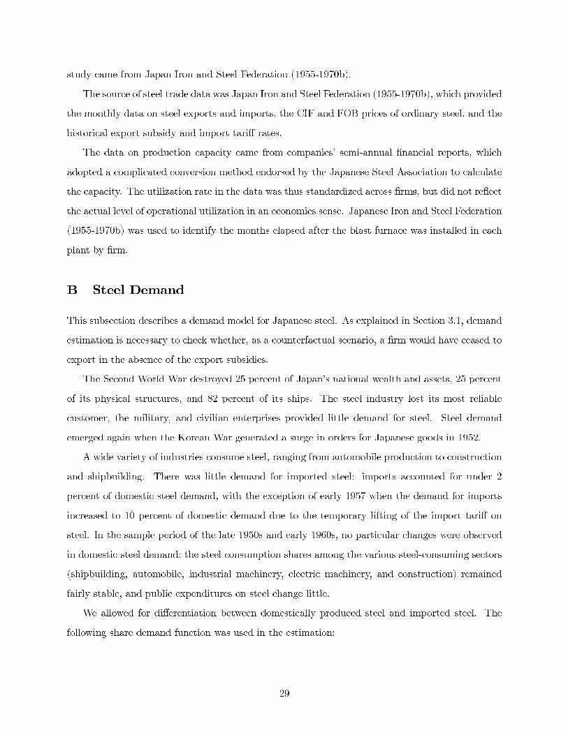
study came from Japan Iron and Steel Federation (1955-1970b).

The source of steel trade data was Japan Iron and Steel Federation (1955-1970b), which provided

the monthly data on steel exports and imports, the CIF and FOB prices of ordinary steel, and the

historical export subsidy and import tariff rates.

The data on production capacity came from companies’ semi-annual financial reports, which

adopted a complicated conversion method endorsed by the Japanese Steel Association to calculate

the capacity. The utilization rate in the data was thus standardized across firms, but did not reflect

the actual level of operational utilization in an economics sense. Japanese Iron and Steel Federation

(1955-1970b) was used to identify the months elapsed after the blast furnace was installed in each

plant by firm.

B Steel Demand

This subsection describes a demand model for Japanese steel. As explained in Section 3.1, demand

estimation is necessary to check whether, as a counterfactual scenario, a firm would have ceased to

export in the absence of the export subsidies.

The Second World War destroyed 25 percent of Japan’s national wealth and assets, 25 percent

of its physical structures, and 82 percent of its ships. The steel industry lost its most reliable

customer, the military, and civilian enterprises provided little demand for steel. Steel demand

emerged again when the Korean War generated a surge in orders for Japanese goods in 1952.

A wide variety of industries consume steel, ranging from automobile production to construction

and shipbuilding. There was little demand for imported steel: imports accounted for under 2

percent of domestic steel demand, with the exception of early 1957 when the demand for imports

increased to 10 percent of domestic demand due to the temporary lifting of the import tariff on

steel. In the sample period of the late 1950s and early 1960s, no particular changes were observed

in domestic steel demand: the steel consumption shares among the various steel-consuming sectors

(shipbuilding, automobile, industrial machinery, electric machinery, and construction) remained

fairly stable, and public expenditures on steel change little.

We allowed for differentiation between domestically produced steel and imported steel. The

following share demand function was used in the estimation:

29

ln

(QD,t

QI,t

)= αd − βd ln

(PD,t

PI,t

)+d,t. (6)

This demand function is derived from a standard CES utility function. Let P and Q be price

and quantity. The subscripts, D and I, stand for domestic and imported steels, respectively (time

subscripts are omitted). The demand error is represented by d. A constant and trend terms are

included in αd. I also included quarterly dummies, and a dummy for the year of 1957, because this is

the year when the tariff was lifted temporarily, presumably because of a surge in domestic demand.

The coefficient βd measures the elasticity of substitutability between domestic and imported steels

perceived in the market. Theory suggests that βd should be greater than one (otherwise, marginal

revenue is negative; see Helpman and Krugman, 1985) The two-stage least-squared method (2SLS)

was used to estimate this demand model. I used, as instruments, input prices (for iron ore and

labor) for the steel industry and the average industry capacity, for cost shifters. These instruments

are likely to correlate with the price ratio in the explanatory variables, but not correlate with d.

Table A presents two demand results: one from the ordinary least squared (OLS) estimation, and

the other from 2SLS. The OLS result is presented for the purpose of comparison. Serial correlation

is often found with time series data. Regression of residuals from each estimation method finds

a significant AR (1) coefficient of 0.4. The table thus reports the results from quasi-differenced

regressions. It makes sense that the 2SLS estimates have larger standard errors. For the 2SLS

estimation, the J statistics would not reject the hypothesis that the instruments are orthogonal to

the error term. Table A also shows averaged first-stage F-statistics for the explanatory power of the

instruments, conditional on the included exogenous variables. They suggest that the instruments

are not weak.

We are interested in the estimate of the elasticity of substitution, βd. The OLS estimate violates

the theoretical constraint that βd ≥ 1, while the 2SLS estimate generates a reasonable magnitude

for the substitution. The comparison stresses the importance of controlling for endogeneity of price.

Based on the demand estimates, we analyzed a firm’s decision to export in the absence of export

subsidies. Figure 2 indicates that a firm does not export if MRF∗ is located below G. In Section

3.3 I discussed that the steel makers competed one another over the choice of output. Under the

Cournot assumption, MRHi is written as

30

MRHi = PD (QD, QI) +Qi,D ·

(∂PD (QD,QI)

∂QD

), (7)

The inverse demand, PD (QD,QI), is derived from a standard CES utility function. Firm i’s

domestic unit sale is Qi,D. One way to find a firm’s export decision in the absence of the subsidy is

to (i) calculate a value of MRHi at the counterfactual output level obtained in Section 5 (denote

this value MRH∗

i ), and then (ii) compare the MRH∗

i with MRF∗. As discussed in footnote 11,

however, we do not have data on Qi,D. Using the theoretical implication discussed in the footnote,

we assume that all six firms had an equal share of the domestic market, and use the industry’s

domestic shipment data to derive Qi,D. The six steel firms in the sample supplied on average

71% of the market for domestically produced steel from 1955 to 1965. I found that the averaged

MRH∗

i (41.75) is lower than the averagedMRF ∗ (49.02). The values in parentheses are in units of

thousands of yen at the January 1960 price. I thus conclude that all the firms in the sample would

have continued exporting. This result is not surprising in hindsight, based on the slight policy

impact reported in Section 5.

C References

Baldwin, R.E. 2003, “Openness and Growth: What’s the Empirical Relationship?” NBER 9578.

Baldwin, R E, and Krugman, P. 1988, “Market Access and International Competition: A Simula-

tion Study of 16K Random Access Memories,” In Empirical Studies of International Trade,

Feenstra, R., ed. 171-197.

Bank of Japan. 1955-1968, Yearbook of Wholesale Price Indices, Tokyo.

Beason, R, and Weinstein, D E. 1996, “Growth, Economies of Scale, and Targeting in Japan

(1955-1990),” Review of Economics and Statistics, 78(2), 286-295.

Benkard, L. 2000, “Learning and Forgetting: The Dynamics of Aircraft Production,” American

Economic Review, 90(4), 1034-1054.

Benkard, L. 2003, “A Dynamic Analysis of the Market for Wide-Bodied Commercial Aircraft,”

Review of Economic Studies, forthcoming.

31

Brander, J A. and Spencer, B J. 1985, “Export Subsidies and International Market Share Rivalry,”

Journal of International Economics, Vol. 18, 83-100.

Dasgupta, P and J. Stiglitz. 1988, “Learning-by-Doing, Market Structure and Industrial and

Trade Policies,” Oxford Economic Papers, 40, 246-268.

Feenstra, R.C. 1986, “Trade Policy with Several Goods and ‘Market Linkages’,” Journal of Inter-

national Economics, 20(3/4), 249-67.

Ghemawat, P. 1985, “Building Strategy on the Experience Curve,” Harvard Business Review,

63(2), March/April, 143-149.

Gruber, H. 1998, “Learning by Doing and Spillovers: Further Evidence for the Semiconductor

Industry,” Review of Industrial Organization, 13, 679-711.

Head, K. 1994, “Infant Industry Protection in the Steel Rail Industry,” Journal of International

Economics, 37, 141-165.

Helpman, E. and P.R. Krugman. Market Structure and Foreign Trade, 1985, MIT Press.

Iron and Steel News, 1955-68, Iron and Steel Almanac, Tokyo, Japan.

Irwin, D and P. Klenow. 1994, “Learning-by-Doing Spillover in the Semiconductor Industry,”

Journal of Political Economy, 102 (6), 1200-27.

Irwin, D and N. Pavcnik. 2001, “Airbus versus Boeing Revisited: International Competition in

the Aircraft Market,” NBER working paper 8648.

Itami, K. 1997, Japanese Steel Industry: Why are they still No.1 in the world?, NTT Press, Tokyo,

Japan.

Itoh, M. and K. Kiyono. 1987, “Welfare-enhancing Export Subsidies,” Journal of Political Econ-

omy, 95(1), 115-37.

Jackson, J.H. The World Trading System, 2000, MIT press.

Japan Iron and Steel Association. 1965, Iron and Steel, Vol. 51, No. 3, Tokyo, Japan.

Japan Iron and Steel Exporters’ Association. 1974, The Twenty Years’ History of the Japanese

Iron and Steel Exporters’ Association, Tokyo, Japan.

32

Japan Iron and Steel Federation. 1955-1970, (a), Yearbook of Iron and Steel Statistics, Tokyo,

Japan.

Japan Iron and Steel Federation. 1955-1970, (b), Monthly Reports on Iron and Steel Statistics,

Tokyo, Japan.

Japan Iron and Steel Federation. 1969, The Ten Years’ History of the Japanese Iron and Steel:

1958-1967, Tokyo, Japan.

Lynn, L. H. 1982, How Japan Innovates: A Comparison with the U.S. in the Case of Oxygen

Steelmaking, Westview Press, Colorado, U.S.A.

Ministry of International Trade and Industry, 1957, White Report, Tokyo, Japan

Miravete, E. 1998, “Infant-industry tariff protection with pressure groups,” International Journal

of Industrial Organization, 16, 749-784.

Miwa, Y. and J.M. Ramseyer. “Japanese Economic Policy and Policy Evaluation—The Case of

”Industrial Policy,” 2001, Economic Review, 52(3), 193-204.

Panagariya, A. “Evaluating the Case for Export Subsidies,” Forthcoming in David Greenaway,

Reanto Flôres and Germán Calfat, ed., Essays in Honor of Mathew Tharakan. Available as

Policy Research Working Paper 2276, World Bank, January 2000.

Patrick, H and Rosovsky, H. 1976, “Japan’s Economic Performance: An Overview,” In Asia’s New

Giant, How the Japanese Economy Works, Patrick, H and Rosovsky, H, ed. The Brookings

Institution, Washington D.C.

Porter, M.E., H. Takeuchi, and M. Sakakibara. Can Japan Compete?, 2000, Perceus, New York.

Rodríguez, F. and D. Rodrik, 2000, “Trade Policy and Economic Growth: A Skeptic’s Guide to

the Cross-National Evidence,” NBER/Macroeconomic Annual, Vol.15(1), 261-325.

Sachs, J.D. and A. Warner. “Economic Reform and the Process of Global Integration,” Brookings

Papers on Economic Activity, 1995 (1), 1-95.

Spence, M. 1981, “The Learning Curve and Competition,” Bell Journal of Economics, 49-70.

33

Spence, M. 1984, “Cost Reduction, Competition, and Industry Performance,” Econometrica,

52(1), 101-121.

Srinivasan, T.N. and J. Bhagwati, 2001. “Outward-Orientation andDevelopment: Are Revisionists

Right?” chapter 1 in Trade, Development, and Political Economy: Essays in Honour of Anne.

O. Krueger, ed. D. Lal and R. Snape. London, Palgrave.

Stiglitz, J. E. 2001, “From Miracle to Crisis to Recovery: Lessons from Four Decades of East Asian

Experience,” Chapter 13 in Rethinking the East Asian Miracle, Stiglitz, J and Yusuf, S. ed.

Oxford University Press, New York.

Thornton, R. A and Thompson, P. 2001, “Learning from Experience and Learning from Others; an

exploration of learning and spillovers in wartime shipbuilding,” American Economic Review,

91(5), 1350-1368.

World Bank. 1993, The East Asian Miracle: Economic Growth and Public Policy, Washington

D.C., Oxford University Press.

Yamamura, K. 1986, “Caveat Emptor: The Industrial Policy for Japan,” Chapter 8 in Strate-

gic Trade Policy and the New International Economics, Krugman, P. ed. The MIT Press,

Cambridge.

Zimmerman, M B. 1982, “Learning Effects and the Commercialization of New Energy Technolo-

gies: The Case of Nuclear Power,” Bell Journal of Economics, 297-310.

34

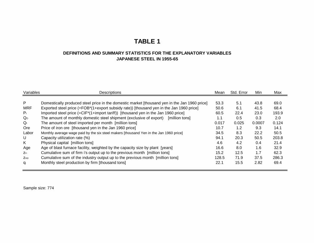
TABLE 1

DEFINITIONS AND SUMMARY STATISTICS FOR THE EXPLANATORY VARIABLESJAPANESE STEEL IN 1955-65

Variables Descriptions Mean Std. Error Min Max

P Domestically produced steel price in the domestic market [thousand yen in the Jan 1960 price] 53.3 5.1 43.8 69.0MRF Exported steel price (=FOB*(1+export subsidy rate)) [thousand yen in the Jan 1960 price] 50.6 6.1 41.5 68.4PI Imported steel price (=CIF*(1+import tariff)) [thousand yen in the Jan 1960 price] 60.5 22.4 23.0 193.9QD The amount of monthly domestic steel shipment (exclusive of export) [million tons] 1.1 0.5 0.3 2.0QI The amount of steel imported per month [million tons] 0.017 0.025 0.0007 0.124Ore Price of iron ore [thousand yen in the Jan 1960 price] 10.7 1.2 9.3 14.1Labor Monthly average wage paid by the six steel makers [thousand Yen in the Jan 1960 price] 34.5 8.3 22.2 50.5U Capacity utilization rate (%) 94.1 20.3 50.5 203.8K Physical capital [million tons] 4.6 4.2 0.4 21.4Age Age of blast furnace facility, weighted by the capacity size by plant [years] 16.6 8.0 1.6 32.9zFi Cumulative sum of firm i's output up to the previous month [million tons] 15.2 12.5 1.7 62.3zIND Cumulative sum of the industry output up to the previous month [million tons] 128.5 71.9 37.5 286.3qi Monthly steel production by firm [thousand tons] 22.1 15.5 2.82 69.4

Sample size: 774

TABLE 2

COST ESTIMATION RESULTS

Model 1 Model 2 Model 3

Base Period of 1955-60 Static

Est. Std. Est. Std. Est. Std.Constant 4.57 ** 0.64 6.79 ** 1.00 0.17 0.15

Labor -0.005 0.02 0.05 ** 0.03 0.19 * 0.12Ore -0.24 ** 0.04 -0.22 ** 0.03 -0.31 ** 0.08

Utilization 0.10 ** 0.04 0.08 ** 0.03 0.12 0.07Capital 0.008 0.01 0.14 ** 0.01 -0.01 0.04

Experience -0.39 ** 0.03 -0.39 ** 0.03 0.18 0.15Spillover 0.01 ** 0.004 0.01 ** 0.005 1.00 1.106

J-statistics (D.F) 1.68 (5) 1.13 (5) 0.26 (5)Coefficient of AR (1) 0.06 0.001 0.78 **

Learning Rates 0.24 ** 0.24 ** -0.13

The number of observations = 774.

* Significance at the 90-percent confidence level.** Significance at the 95-percent confidence level.

Notes:The firm and year fixed components are included in the estimations (not reported).J statistics provide a test of overidentifications. A coefficient of AR(1) is constructed by first obtaining an estimatedcoefficient of the lagged residual for each firm, and taking an average of them. The learning rate is the magnitude of the cost drop with doubling the experience. It is obtained as 1 minus 2 to the power of the experience coefficient.

TABLE 3

MODEL PREDICTIONS

Estimated Actual Industry Largest firm's Smallest Firm's Industry Largest firm's Smallest Firm's

Outputs (M tons) (Yawata) Share (%) (Kobe) Share (%) Outputs (M tons) (Yawata) Share (%) (Kobe) Share (%)1955 9.38 24.45 4.15 9.41 24.48 4.141956 11.05 23.13 4.04 11.11 23.18 4.041957 12.51 22.83 4.22 12.57 22.92 4.201958 12.03 23.59 4.15 12.12 23.74 4.141959 16.52 23.70 4.30 16.63 23.81 4.301960 21.93 22.59 4.37 22.14 22.78 4.381961 27.97 21.47 4.25 28.27 21.65 4.231962 27.48 20.78 4.44 27.55 20.85 4.431963 31.26 19.46 4.58 31.50 19.56 4.591964 39.31 18.98 4.33 39.80 19.14 4.341965 41.14 18.81 5.50 41.16 18.85 5.49

Outside-of-the-Sample Predictions

Estimated Actual Industry Largest firm's Smallest Firm's Industry Largest firm's Smallest Firm's

Outputs (M tons) (Yawata) Share (%) (Kobe) Share (%) Outputs (M tons) (Yawata) Share (%) (Kobe) Share (%)1966 47.73 18.78 5.58 47.78 18.78 5.581967 61.96 18.65 5.41 62.15 18.67 5.411968 66.78 18.57 5.41 66.89 18.55 5.42

Note: For the sake of brevity, I only report market shares of the largest and smallest firms. The largest steel maker in 1955-68 was Yawata, and the smallest was Kobe. Market shares prediction of the other firms show similar degree of accuracy.

TABLE A

DEMAND ESTIMATION RESULTSwith AR (1) Error Correction

OLS 2SLSEst. Std. Err. Est. Std. Err.

Constant 0.84 ** 0.11 3.11 ** 0.33Log of (PD/PI) 0.26 ** 0.03 4.46 ** 1.50Trend 0.06 ** 0.01 0.24 1.12Dummy on Year 57 -0.46 ** 0.09 -1.18 0.94Dummy on Q2 0.08 0.06 0.38 1.15Dummy on Q3 0.20 ** 0.06 0.83 1.24Dummy on Q4 0.04 0.06 0.01 1.08AR 1 coefficients 0.386 0.388R-squared 0.50 -J-statistics (D.F) - 0.60 (2)1st-stage F-statistics - 15.96 **No. obs. 132 132

** Significance at the 95-percent confidence level.

Notes:Equation (6) in Appendix B is estimated. The dependent variable is the logarithm of a quantity ratio; quantity of domestic steel, divided by import quantity. Estimates are based on a regression from quasi-differenced variables. J statistic provides a test of overidentifying restrictions. First-stage F statistic provides the average explanatory power of the instruments, conditional on the included exogenous variables.

FIGURE 1Steel Production & Export Subsidy

1931-1969

ExportSubsidy

Production

AverageSubsidy Rate

(%)

SteelProduction

(Million tons)

0.0

0.5

1.0

1.5

2.0

2.5

3.0

3.5

4.0

4.5

5.0

1931 1933 1935 1937 1939 1941 1943 1945 1947 1949 1951 1953 1955 1957 1959 1961 1963 1965 1967 19690

10

20

30

40

50

60

70

80

90

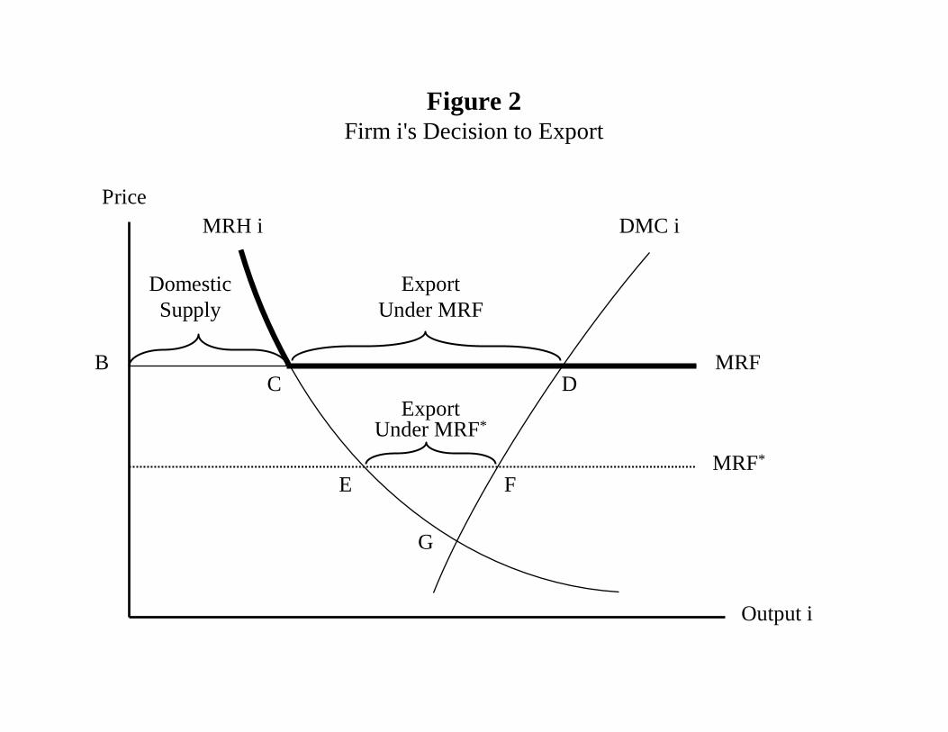
Figure 2Firm i's Decision to Export

Price

Output i

MRF

MRF*

Export Under MRF*

Export Under MRF

Domestic Supply

MRH i DMC i

DB

C

E F

G

FIGURE 3VARIOUS COST MEASURES

MC

AC

DMC

Price

20

30

40

50

60

70

80

90

100

110

1955 1956 1957 1958 1959 1960 1961 1962 1963 1964 1965

1,000 Yen per ton

(in Jan 1960)

FIGURE 4Policy Impacts of Subsidy:

Ratios of Industry Outputs with Subsidy Relative to without Subsidy

Full Spillover:Output w/ subsidy

Output w/o subsidy

Actual outputOutput w/o subsidy

Doubled Subsidy:Output w/subsidy

Output w/o subsidy

0.98

0.99

1.00

1.01

1.02

1.03

1.04

1.05

1955 1956 1957 1958 1959 1960 1961 1962 1963 1964 1965 1966 1967 1968

Ratio of outputs with subsidy towithout subsidy