Embed Size (px)
Citation preview


ARCHITECTURE ENGINEERING and CONSTRUCTION
International Journal of Architecture, Engineering and Construction
Editor-in-Chief Xueqing Zhang
Hong Kong University of Science and Technology, Hong Kong
Associate Editors Bryan T. Adey
ETH Zurich, Switzerland Dale Clifford
Carnegie Mellon University United States of America
Garrick E. Louis University of Virginia United States of America
Corrado Lo Storto University of Naples Federico II Italy
Shouqing Wang Tsinghua University, China
Zhong You University of Oxford United Kingdom
Honorary Editor Hojjat Adeli
Ohio State University United States of America
Editorial Advisory Board Simaan M. AbouRizk
University of Alberta, Canada Thomas Bock
Technical University of Munich, Germany Makarand Hastak
Purdue University, United States of America Shyh-Jiann Hwang
National Taiwan University, Taiwan Timothy J Ibell
University of Bath, United Kingdom Edward J Jaselskis
North Carolina State University, United States of America Kiyoshi Kobayashi
Kyoto University, Japan Thomas Kvan
University of Melbourne, Australia Kincho H Law
Stanford University, United States of America Christopher K Y Leung
Hong Kong University of Science and Technology, Hong Kong Yuan Li
Shanghai Jiao Tong University, China Ali Maher
Rutgers University, United States of America Campbell R. Middleton
University of Cambridge, United Kingdom Peter W. G. Morris
University College London, United Kingdom George Ofori
National University of Singapore, Singapore Feniosky Pena-Mora
Columbia University, United States of America Qinghua Qin
Australian National University, Australia Klaus Rueckert
Technical University of Berlin, Germany Surendra P. Shah
Northwestern University, United States of America Miroslaw Skibniewski
University of Maryland, United States of America Nobuyoshi Yabuki
Osaka University, Japan
General Information
International Journal of Architecture, Engineering and Construction
http://www.iasdm.org/journals
Aim and Scope International Journal of Architecture, Engineering and Construction (ISSN 1911-110X [print] and ISSN 1911-1118 [online]), IJAEC, is published by the International Association for Sustainable Development and Management (IASDM). IJAEC is a scholarly peer-refereed journal that promotes scientific and technical advances as well as innovative implementations and applications in the architecture, engineering and construction of the built environment. IJAEC publishes original research papers, state-of-the-art review papers, novel industrial applications, insightful case studies and objective book reviews in a broad scope of topics related to these areas.
AEC Forum IJAEC provides an online AEC Forum, which is an interactive platform for international business organizations, public agencies, civil societies and academia to disseminate and exchange information, and to discuss on various issues in architecture, engineering and construction. This forum can be accessed at http://www.iasdm.org/forums.
Manuscript Submission To register as a new user, log onto the system, and submit manuscripts, go to http://www.iasdm.org/journals/ index.php/ijaec/login. Manuscripts under review, accepted for publication, or published elsewhere are not accepted. Written permissions from the original publisher for both print and online reproduction must be provided along with the manuscript if using previously published figures and/or tables. Discussion is welcomed for all materials published in IJAEC and will be considered individually for publication or private response. Detailed instructions to authors can be obtained online at http://www.iasdm.org/journals/index.php/ijaec/ about/authors.
Length Requirements Although there is no strict limit on the maximum number of words or word-equivalent, it is recommended 10,000 for papers and 3,000 for book reviews, discussions and closures.
E-mail Updates Abstract information for IJAEC is electronically available at http://www.iasdm.org/journals/index.php/ijaec/issue. Keep up with new publications from IJAEC by joining IJAEC’s free e-mail alerting service through http://www.iasdm.org/journals/index.php/ ijaec/login and journal table of contents (with links to abstract) and latest news will be sent to you.
Copyright All rights reserved. Apart from any fair dealing for the purposes of research or private study, or criticism or review, no part of this publication may be reproduced, stored or transmitted in any form or by any means electronic, mechanic, photocopying, recording or otherwise, without the prior permission in writing form from the author and the publisher.
Disclaimer Papers and other contributions and statements made or opinions expressed in the journal are published on the understanding that the author of the contribution is solely responsible for the opinions expressed in it and that its publication does not necessarily imply that such statements and/or opinions are or reflect the views of the journal or the IASDM.
ARCHITECTURE ENGINEERING and CONSTRUCTION

ARCHITECTURE ENGINEERING and CONSTRUCTION
International Journal of Architecture, Engineering and Construction
Volume 1, Number 3 September 2012
Managing Editor Catherine Wang
International Association for Sustainable Development and Management, Canada
Technical Editors Hui Gao
Hohai University, China Venkata Ramana Gadhamshetty
Rensselaer Polytechnic Institute, United States of America
121 134 142 155 163 174 183
Research Papers Identifying Project Value Interests: A Binary Logit Model Molly Gunby, Ivan Damnjanovic and Stuart Anderson A Method for Calculating Cost Correlation among Construction Projects in a Portfolio Payam Bakhshi and Ali Touran Developing an Effective Bridge Facilities Management Optimization Model Xueqing Zhang Shelters of Sustainability: Reconfiguring Post-tsunami Recovery via Self-labor Practices Chamila T. Subasinghe Industrial Application Automated Productivity Measurement Model of Two-dimensional Earthmoving-equipment Operations Ronie Navon, Simon Khoury, and Yerach Doytsher Case Study Environmental Evaluation of Abrasive Blasting with Sand, Water, and Dry Ice Lauren R. Millman and James W. Giancaspro Book Review Modern Construction: Lean Project Delivery and Integrated Practices/ISBN: 978-1-4200-6312-7 David J. Kelly

International Journal of Architecture, Engineering and ConstructionVol 1, No 3, September 2012, 121-133
Identifying Project Value Interests: A Binary Logit Model
Molly Gunby, Ivan Damnjanovic∗, Stuart Anderson
Zachry Department of Civil Engineering, Texas A&M University, College Station, TX 77843, United States
Abstract: Identifying ways in which projects add value to owner organizations is an important part of projectdevelopment and delivery. In addition to standard functional and delivery requirements there are a number ofother value-adding attributes that are sometimes difficult to communicate or may not be fully evident to theowner organization. These value adding attributes, or value interests, can be difficult to identify, define, andcommunicate because too often they are misunderstood, overshadowed by budget or schedule, or too broadlydefined for implementation. To address this issue, the Construction Industry Institute in the United Statescommissioned the development of a method to identify owner value interests, facilitate their communicationbetween stakeholders, and identify engineering and construction response strategies. This paper presents abinary logit regression model for identifying initial value interests based on project characteristics. The modelwas developed using survey data and tested to ensure that it provides results that are logical and comparableto recommendations made by survey participants.
Keywords: Value interests, value objectives, project value, logit model
DOI: 10.7492/IJAEC.2012.014
1 INTRODUCTION
Effective communication of project expectations is crit-ical to project success. A full range of unique projectvalue-adding attributes (not only cost and schedule ob-jectives) must be identified and communicated to allmembers of the project team. Ineffective communica-tion of value objectives can lead to misalignment withinthe owner’s project team, as well as between the ownerand contractor.Project value-adding attributes are often not prop-
erly communicated. Part of this difficulty stems fromthe fact that the value-adding project attributes, orvalue interests, are often misunderstood or even maynot be fully recognized by the owners. As a result, theengineering and construction (E&C) providers are leftto make their own assumptions regarding owner valueinterests to fill in their knowledge gaps. Inevitably,this unintentional misalignment between the owner’sexpectations and the E&C providers’ understanding ofthe project’s values leads to conflicts, delays, and aless-than-satisfied owner. Another factor that compro-mises this communication is that the value interestsare often too broadly defined. It is not uncommon foran owner to define their value interests as cost, sched-ule, and quality. While these broad components areunquestionably critical to successful project execution,they do not convey the complexity of the owner’s needs
nor the specificity necessary for an E&C provider todevelop an effective response strategy. For example,meeting the specified project cost may be critical toan owner. Or, conversely, meeting the specified costmay be important but the owner may be flexible withthe cost if it enhances achievement of other, more criti-cal, value interests. Thus, simply communicating cost,by itself, as a value interest does not convey the truevalue desires of the owner. Similarly, there are count-less ambiguous applications of quality in capital projectdelivery.
In order to identify project value interests, it is firstnecessary to understand what drives them. An owner’scharacteristics (company size, business strategy, etc.)tend to be global and may not dictate what the valueinterests are for a specific project. In addition, a singleowner may engage in many different types of projectsand the value interests of one project may not be thesame as the value interests of another. Instead, valueinterest drivers may be characteristics of the projectitself such as the size of the project, the extent ofnew technology required, or the activities for which theE&C provider is responsible. For example, the valueinterests for a refinery project may be more driven bythe project location and level of technology than howlarge the company is or whether the company is Com-pany X or Company Y. In addition, characterization ofan owner is impractical, as a sufficient number of “sim-
*Corresponding author. Email: [email protected]
121
Gunby et al./International Journal of Architecture, Engineering and Construction 1 (2012) 121-133
ilar” owners need to be identified for data collectionpurposes and the resulting model would only be imple-mentable to those owners. Thus, identifying projectcharacteristics that have the greatest influence on var-ious project value interests would enable owners to se-lect and communicate the value interests appropriateto a specific project. It is important to note that theowner’s strategies for a particular project are not solelydetermined by project characteristics; organizationalobjectives and market conditions play an importantrole as well. However, as these factors vary and are of-ten unpredictable, they were not explicitly consideredin this study.In 2008, the Construction Industry Institute (CII) in
the United States initiated a research project to de-velop a methodology to assist in the identification andcommunication of project-specific value interests andidentify an appropriate E&C response (Damnjanovicet al. 2011). The study team consisted of three aca-demic members and seventeen industry professionals.The industry experts on the team had extensive ex-perience with both the engineering/construction andbusiness requirements of a project. Their backgroundsincluded presidents and vice presidents, project anddivision managers, directors of operations and busi-ness process improvement, among others. The finalproduct of the research effort was a Microsoft Ex-cel? file, which contains a value interest identificationmodel and provides guidance on developing value in-terest measurement units, setting their required levelsand specifying trade-offs among them (Damnjanovicet al. 2010). This paper presents the methodology fordeveloping and validating the CII value interest iden-tification model. More specifically, it describes fourprimary tasks:
1. Enumeration and definition of major elements ofstudy: The value interests and project character-istics included in this study were identified anddefined.
2. Survey of industry: A survey was distributed toowner and contractor companies to obtain empir-ical data that was used to develop and confirmthe relationship between project characteristicsand value interests.
3. Model development: A binary logit model was es-timated using the maximum likelihood method.The estimated parameters were then used to de-velop a model, which could predict the applica-bility of a value interest to a specific combinationof characteristics.
4. Model validation: The model was validated to en-sure its value interest recommendations are real-istic and comparable with the recommendationsmade by the survey participants. This was ac-complished by comparing a randomly selectedsubset of survey responses to the recommenda-tions made by the model for the same projectdescription.
This methodology is presented in further detail inthe following sections: first, section 2 provides a sum-mary of relevant research efforts including studies intoproject value objectives and the application of discretechoice analysis and the binary logit model. Next, theMethodology gives a brief overview of the five primarytasks performed in this study. In section 4, the firstof these tasks, the enumeration and definition of valueinterests and project characteristics are presented. Fol-lowing this, section 5 expands on the method of datacollection including the development and distributionof an industry survey, the type of data received andhow it was prepared for modeling, and how the surveydata was checked for consistency among different re-sponse sources. An overview of the binary logit model,model specification method, and a sampling of the pa-rameter estimates obtained in this study are given insection 6. The two approaches used to validate themodel - random sampling of survey responses and afield test - are discussed in section 7. Section 8 pro-vides some implications of the products of this studyincluding conclusions obtained from the survey dataitself, implications of the model parameter estimates,and a discussion of some unexpected observations. Fi-nally, section 9 summarizes this study and underscoreshow the model can be useful to both owners and E&Cproviders during all phases of project development anddelivery.
2 BACKGROUND
2.1 Project Value Objectives
Though it seems the most basic part of project devel-opment, identification and communication of projectobjectives are not always a simple task as project ob-jectives are tied to both the project requirements andstrategic needs of the organization (Griffith and Gib-son Jr. 1997). Part of the difficulty of developingand achieving objectives occurs because objectives arefrequently ambiguously defined or unachievable goalsspecified. Lewis (2007) stated that objectives mustbe SMART: specific, measureable, attainable, realis-tic, and time-limited. Further, he warned that anobjective should describe the result, rather than howto achieve it. Misalignment among project stakehold-ers can also create complications in the developmentand achievement of project objectives. Since projectteam members and stakeholders come from differentdivisions within organizations, it is natural that theybring with them the priorities or expectations relevantto their experience and functional area (Griffith andGibson Jr. 1997). Thus, alignment of all members ofthe project team behind a common set of project objec-tives requires reconciling many different priorities andneeds. Griffith and Gibson Jr. (1997) identified tenfactors that influence alignment during the pre-projectplanning phase and developed a tool, the Alignment
122
Gunby et al./International Journal of Architecture, Engineering and Construction 1 (2012) 121-133
Thermometer, to gauge the project team’s success inaddressing the ten factors.The achievement of budget, schedule, and technical
objectives is no longer the only criterion for the evalua-tion of a successful project. Shenhar et al. (1997) iden-tified four dimensions that should be considered whenassessing project success. One of these, naturally, re-lates to the achievement of project constraints, includ-ing cost and time. However, the other three dimensionsgauge success based on the impact of the project on thecustomer, end-user and organization, and whether theproject positions the organization for future opportu-nities. Atkinson (1999) suggested there were at leastthree other aspects of project success criteria (beyondcost, schedule, and quality) that should be considered:the technical attributes of the project, the benefits tothe organization, and the benefits to the stakeholdercommunity. Thus, there is a shift occurring in howproject success is defined from simply meeting projectconstraints, to delivering a project that provides themaximum value to an organization.As a result of this shift, there has been significant re-
cent research into identifying the project practices andmanagement strategies that can add value and maxi-mize the probability of project success. Berman (2006)developed the Speed2V alueTM Road Map, a compre-hensive process designed to help organizations focus onand achieve the strategic value of a project. The pro-cess is broad enough to be used in any industry andprovides guidance on identifying the project’s valuedrivers, documenting measures to gauge project suc-cess, and following through to maximize the project’sbenefits during its whole life cycle, among other activ-ities. The Road Map does not provide recommenda-tions of specific project values but, instead, providesguidance to assist an organization in developing theirown. Cooke-Davies (2002) identified twelve factors es-sential to project success including those related torisk management and ownership, scope changes, align-ment with corporate objectives, and continuous im-provement through lessons learned, among others. Thefactors were grouped according to management suc-cess (achievement of time and cost), project success(achievement of stakeholder benefits), and corporatesuccess (consistently successful projects).The CII has also been a sponsor of a number
of research projects investigating value-adding prac-tices. The V alue Management Toolkit (O’Connoret al. 2003) is a comprehensive tool that pro-vides guidance on value-adding practices. Thetoolkit includes guidance on selecting the appropri-ate practice and the optimal time to implementit. The Cost-Schedule Trade-off Tool (Gokhaleet al. 2006) identifies techniques to meet specificcost- or schedule-driven objectives at each projectphase. Owner′s Role in Project Success (Griffisand Bates 2006) developed a tool to help ownersidentify the project areas in need of greater atten-
tion. Planning for, Facilitating and EvaluatingDesign Effectiveness (O’Connor et al. 2007)and Maximizing Engineering V alue (O’Connor andSingh 2009) were developed to assist organizations inidentifying design and engineering strategies that en-hance the achievment of project objectives and max-imize the value of the project. These resources havesignificantly advanced the practical knowledge of value-added design and management. However, there is stilllacking a methodology that can identify and recom-mend a unique set of value-adding project elementsbased on specific project characteristics. Thus, thereis a need to collect data and develop a model that cancapture preferences and relate project charateristics tovalue interests.When conducting surveys to capture choice data, the
selections available to survey participants are often lim-ited to a number of discrete and unordered options.Frequently, this is the case with surveys on the usage ofhousehold products, choices of travel modes or routes,and preferences of news and media sources. These sur-veys can generate valuable information for companieson the criteria people use to evaluate and choose amongtheir products or allow them to tailor their advertise-ment to a specific audience. Analysis of past choicebehavior can be used to predict future behavior suchas how a consumer will respond to a new product orhow likely people will be to use a new product or aproject such as toll road.
2.2 Discrete Choice Analysis
Discrete Choice Analysis (DCA) is a type of methodused to model ordered and unordered choices. TheDCA outcome is the probability that a particularchoice will be made given the characteristics of thealternatives. According to Ben-Akiva and Lerman(1985), DCA was used as far back as the 1960’s toexamine binary travel mode preferences and its uti-lization expanded significantly in the 1970’s to in-clude multi-choice (more than two) modal preference,vehicle ownership, and other transportation relatedchoices. Wassenaar and Chen (2001) also used thisanalysis technique to develop a demand model for in-tegration into decision-based design framework. Riversand Jaccard (2005) used DCA to analyze steam gen-eration technology preferences among Canadian indus-trial companies and integrate the results into a hybridenergy-economy model to investigate the effects of dif-ferent energy policies. In the context of this study,DCA was selected as an appropriate method to analyzethe industry survey data. The data collected includedordered, multi-level project descriptions and discretevalue interest choices provided by high level projectmanagers. Application of DCA provided the proba-bility of applicability of a value interest for a givencombination of project descriptors.The method used to perform a choice analysis de-
123
Gunby et al./International Journal of Architecture, Engineering and Construction 1 (2012) 121-133
pends on several factors, in particular the type of de-pendent or outcome variables. When the outcome vari-able is limited to a set of discrete or binary selections,ordinary linear regression is not a suitable option. Thisis because when the dependent variable is dichotomous,linear regression frequently results in predicted prob-abilities greater than 1 and less than 0. Instead, thelogistic regression model is a widely accepted alterna-tive for this type of numerical analysis (Hosmer andLemeshow 2000). The logit model ensures realisticpredicted probabilities, between 0 and 1, as well ashas the appealing attribute of computational simplic-ity (Kennedy 2003).The logit model has been applied extensively in en-
gineering and construction studies. Kenley and Wil-son (1986) used logistic regression to develop a post-completion cash flow analysis model, as well as to showthat it is the unique character of a project that createsvariance from one project to another and not a sys-tematic error. The implication of their study is thatthe generally accepted s-shaped cash flow models thatreflect the industry average are not adequate for cashflow prediction of a unique project. Mohamad et al.(1997) used a mixed logit model (discrete and contin-uous dependent variables) in a two-stage approach topavement performance that considered the interactiveeffects of maintenance and pavement condition. Usinglogistic regression, Phua (2006) showed the adoption ofpartnering or collaborating within the construction in-dustry is largely influenced by whether the practice isencouraged by industry norms, rather than by the po-tential benefits of the practice perceived by individualfirms.The logit model has also been used to a great ex-
tent in the evaluation of construction site safety. Weil(2001) used this modeling method to show how repet-itive site inspections influence compliance with OSHAsafety standards and Seixas et al. (2001) used it toidentify the causalities (task, tool use, location charac-teristics, etc.) of noise levels exceeding OSHA permis-sible limits to which electricians are exposed. Li andBai (2006) used logistic regression to examine how dif-ferent traffic control devices reduce the occurrence ofcrashes in construction zones.
3 METHODOLOGY
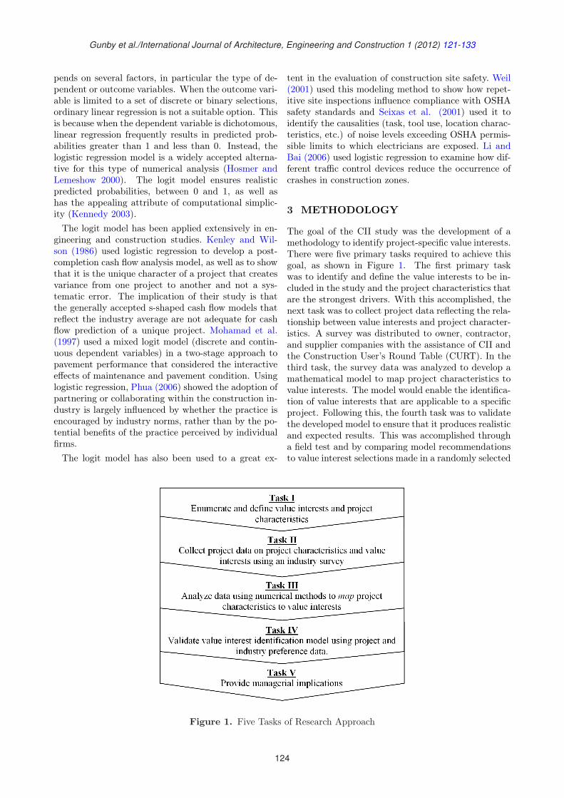
The goal of the CII study was the development of amethodology to identify project-specific value interests.There were five primary tasks required to achieve thisgoal, as shown in Figure 1. The first primary taskwas to identify and define the value interests to be in-cluded in the study and the project characteristics thatare the strongest drivers. With this accomplished, thenext task was to collect project data reflecting the rela-tionship between value interests and project character-istics. A survey was distributed to owner, contractor,and supplier companies with the assistance of CII andthe Construction User’s Round Table (CURT). In thethird task, the survey data was analyzed to develop amathematical model to map project characteristics tovalue interests. The model would enable the identifica-tion of value interests that are applicable to a specificproject. Following this, the fourth task was to validatethe developed model to ensure that it produces realisticand expected results. This was accomplished througha field test and by comparing model recommendationsto value interest selections made in a randomly selected
Figure 1. Five Tasks of Research Approach
124
Gunby et al./International Journal of Architecture, Engineering and Construction 1 (2012) 121-133
Table 1. Sample of Five Value Interests with Definitions
Value Interest DefinitionExperience with reg-ulatory compliance
The demonstration of experience regarding required technical specifications, qualifications,performance, and operability in order to meet a federal, state, county or local law.
Optimum cost Balancing the project cost objectives against all other value interests to obtain the bestoverall achievement of the project objectives.
Optimum schedule Balancing the project schedule objectives against all other value interests to obtain the bestoverall achievement of the project objectives.
Process flexibility The degree to which the project design allows for variation in capacity or composition tomaximize the efficiency of the process, minimize future expansion costs, and meet variationin production requirements resulting from changes in the marketplace.
Uninterrupted busi-ness
The ability of a facility to continue operations to the degree specified by the owner whileundergoing or adjacent to major renovations or additions.
set of survey responses. Finally, the last task was tosummarize what was learned through this exercise interms of how a manager or executive can benefit fromthis knowledge.
4 ENUMERATION AND DEFINITIONOF TERMS
4.1 Value Interests
Value interest represents an owner defined project at-tribute that add some measure of value to the ownerorganization (Damnjanovic et al. 2010). A value inter-est could be a typical project requirement or it could bea feature that is specific to a particular type of projector industry. The common thread between all valueinterests is the added value to the owner. For exam-ple, cost and schedule are value interests as their out-comes directly add/reduce the value of the project tothe owner organizations. Energy efficiency, public im-age, and the design team’s level of experience are alsovalue interests. Initially, drawing from their extensiveprofessional experience, the industry experts on the CIIstudy team identified 70 value interests. In addition,the team performed a literature review to identify po-tential value interests; however, all value interests iden-tified during the literature review were already presentin some form in the study team’s list. Through severalreview and revising iterations, redundant value inter-ests were eliminated so that the final list contained 48
terms. Table 1 provides a sample of five value interestsand definitions. All of the 48 value interests and theirdefinitions can be found in the report “A StandardizedApproach to Identifying and Defining Owner Value In-terests and Aligning the E&C Response” (Damnjanovicet al. 2011).
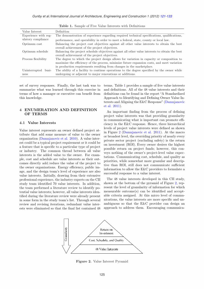
An important finding from the process of definingproject value interests was that providing granularityin communicating what is important can promote effi-ciency in the E&C response. Hence, three hierarchicallevels of project value interests were defined as shownin Figure 2 (Damnjanovic et al. 2011). At the macroor broadest level, the overriding priority of nearly everyprivate sector project (excluding safety) is the returnon investment (ROI). Every owner desires the highestpossible return on project funds; however, this con-veys nothing of the owner’s project-level value expec-tations. Communicating cost, schedule, and quality aspriorities, while somewhat more granular and descrip-tive than ROI, still does not communicate sufficientinformation to allow the E&C providers to formulate asuccessful response to a value interest.
The 48 value interests developed in this CII study,shown at the bottom of the pyramid of Figure 2, rep-resent the level of granularity of information for whichmeasurable outcome(s) can be identified and accept-able criteria assigned. At this micro level of commu-nications, the value interests are more specific and un-ambiguous so that the E&C provider can design anapproach to address them. Encouraging communica-
Figure 2. Value Interest Pyramid
125
Gunby et al./International Journal of Architecture, Engineering and Construction 1 (2012) 121-133
Table 2. Five Choice Levels for the Technology Characteristic
Choice Level Choice Description1 It is common and/or repeatable, the owner has extensive experience with it, and there are
no anticipated complications.2 It will require modification/scaling of existing technology, the owner has extensive experience
with it, and there are no anticipated complications.3 It has average maturity and/or complexity and the owner has some (but not extensive)
experience with it.4 It has limited commercialization and/or unknown scalability and the owner has limited ex-
perience with it.5 It is ground-breaking with no previous commercialization and the owner has no experience
with it.
tion between the owner and the E&C provider at thislevel of granularity represents the larger goal of thismodel.
4.2 Project Characteristics
It was also necessary to identify initial project char-acteristics that would likely represent the strongestdrivers for selection of value interests. The charac-teristics must be general enough to be applicable toall projects and industries but also specific enough tocapture the features that make a project and its valueinterests unique. In an exercise similar to the valueinterest development, the industry experts of the CIIstudy team identified and defined twelve key projectcharacteristics: industry, location, size (in U.S. dol-lars), degree of technology, complexity, project nature,type of project (scope of work), level of owner’s involve-ment in project execution, strategic importance to theowner, cost driven, schedule driven, and the degree ofregulation. In addition, five possible choices, or levels,were defined for eleven of the characteristics. Theselevels signify an increasing scale from a low value ofthe characteristic to a high value of the characteristic.For example, the five levels of technology are shown inTable 2 (Damnjanovic et al. 2011). Since the indus-try characteristic represents the industry of the project(e.g., pharmaceutical, oil and gas, or manufacturing),
the levels of this variable are categorical and cannot beplaced in a scaled order. Therefore, this characteristicwas given eight unordered levels. Damnjanovic et al.(2011) provides the definitions of all twelve projectcharacteristics and their levels.
5 COLLECTION OF PROJECT DATA
5.1 Industry Survey
With the assistance of CII and CURT, a survey was dis-tributed to owner, contractor, and supplier companiesduring the spring and summer of 2009. The intentionof the survey was to capture both the owner’s and thecontractor’s perspectives on what drives project valueinterests. It is important to note that the contractorswere instructed to answer the survey questions from theperspective of the owner or, in other words, as if theywere the owner. In fact, E&C providers (contractors)that have participated in this study have substantialexperience with owner organizations and the value in-terests they seek in their projects.The survey was sent to over 100 CII and CURT com-
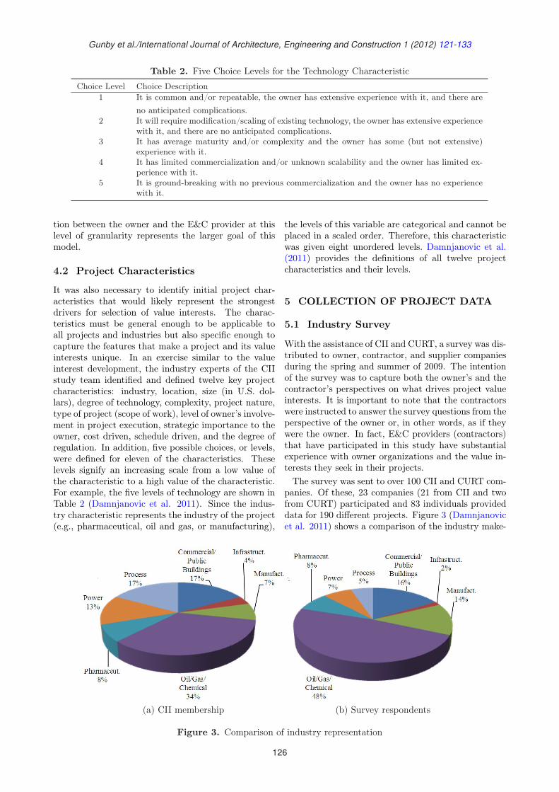
panies. Of these, 23 companies (21 from CII and twofrom CURT) participated and 83 individuals provideddata for 190 different projects. Figure 3 (Damnjanovicet al. 2011) shows a comparison of the industry make-
(a) CII membership (b) Survey respondents
Figure 3. Comparison of industry representation
126
Gunby et al./International Journal of Architecture, Engineering and Construction 1 (2012) 121-133
up of CII owner members and the survey responsesreceived from owner companies. The responses andCII membership of contractors was not included in thiscomparison since they may engage in projects in manydifferent industries.As shown, the representation of the pharmaceutical,
commercial/public buildings, and infrastructure indus-tries were the same or very similar. However, theoil/gas/chemical and manufacturing industries wereover-represented in the survey responses. This was con-sistent with CII membership and the type of projectsin which CII members are involved.
5.2 Survey Data
The survey consisted of three steps. In the first step,the participant was asked to describe a completedproject with which they have had experience usingthe characteristics. The characteristic levels were pre-sented to the participant as multiple-choice options.Next, they were asked to review the list of 48 valueinterests (with definitions) and choose the ten theybelieve would have been most relevant to the projectthey described. Finally, the participants were askedto weigh the value interests by assigning a number be-tween 0 and 100 to reflect their relative applicabilityto the project. The weights of the ten value interestswere required to sum to 100.Each project response provided: (1) choices for
twelve project characteristics, describing the project,and (2) ten weighted value interests, describing whatvalue interests were relevant for that project. Theseresponses were then processed to provide a data setthat was used for modeling purpose. To this aim, twounique features of the data set were considered: (1)project characteristics choices are defined on an ordinalscale measurement for all but one characteristic; and(2) value interest responses specify an empirical proba-bility mass function for a given combination of projectcharacteristics, where weights correspond to the likeli-hood of each value interest being selected.An ordinal scale of measurement for project charac-
teristics was considered using five choice levels repre-sented on an increasing scale. Each level was thereforeassigned a value from 1 to 5 with 1 representing thelowest level and 5 representing the highest (see Ta-ble 2). Since the eight choices for industry were notordered, they were treated on a nominal scale.A total of 190 project responses were re-sampled
to increase the robustness of the project value inter-ests estimates. In this effort, an empirical distributionof the observed response data defined using value in-terests weights as an approximating distribution wasused (Efron and Tibshirani 1986). Using these valueinterest weights, the responses were re-sampled and thedata set expanded in an operation similar to statisti-cal bootstrapping. For example, a re-sample from theempirical probability mass distribution shown in Ta-
bles 3 and 4 (Damnjanovic et al. 2011) would producea new sample of 100 responses with identical levels ofproject characteristics (location, size, etc.). The resultof this re-sampling exercise was an increased data set of19,000 responses in which a project defined by the lev-els of project characteristics (location, size, etc.) wereassociated with only one choice of value interests.
Table 3. Example Survey Response (1)
Project Characteristic Selected Level
Industry Type 8Location 1Size 3Technology 4Complexity 2Project Nature 3Type of project 1Owner Involvement 1Strategic Importance 1Cost Driven 5Schedule Driven 1Regulation 2
Table 4. Example Survey Response (2)
Selected Value Interest Assigned Weight
Optimum cost 20%Design team experi-ence/competency
10%
Standard work processes 5%Constructability 5%Allocate/Share risks 10%Meet the schedule objective 15%Product Quality 10%Procurement competency 5%Single point of responsibilityfor project execution
5%
Meet the cost objective 15%Sum 100%
5.3 Comparison of Responses
By coincidence, exactly half of the project responsescame from owners and the other half from contractorsand suppliers. To ensure the inclusion of contractorsand suppliers did not skew the data, their value interestchoices were compared with those of the owners. Thecomparison was performed by finding the difference inthe frequencies with which each group chose each valueinterest, as a percentage of the group’s total number ofchoices. The result showed the value interest selectionsmade by each group were strikingly similar. For 39 ofthe value interests, the difference in frequencies wasless than one percent. The greatest difference was ob-served with the value interest “design team experience”;the owners selected this value interest approximately2.3% of the time and the contractors and suppliers se-lected it approximately 5.8% of the time, a difference
127
Gunby et al./International Journal of Architecture, Engineering and Construction 1 (2012) 121-133
of about 3.5%. The mean difference of all value inter-ests was 8.1× e−18, with a 95% confidence interval of ±1.7%. Thus, there was no indication that the differencebetween the two groups’ selections was statistically sig-nificant or that inclusion of contractors and suppliersskewed the data.
6 DATA ANALYSIS
6.1 Binary Logit Model
The logit model is part of a family of generalized linearmodels (GLM). The expected value E(Y ) of a randomvariable, Y , can be expressed in terms of a set of de-pendent, or explanatory, variables as:
E(Y ) = µ =n∑
i=1
βixi (1)
where β represents a vector of n unknown parametersand x is a vector of explanatory variables. As shown,the expected value of the random variable is linearlyrelated to its predictors. The logit model follows asimilar form, however, its expected value is not lin-early related to its predictors. Instead, the expectedvalue is related to its predictors through the use of alink function, η, where η is linearly related to the pre-dictors (Liao 1994). Rewriting Eq. (1) for the logitmodel using this link function gives:
η =n∑
i=1
βixi (2)
where the expected value of the logit model is relatedto η through the expression:
η = logµ
(µ− 1)(3)
Using Eqs. (2) and (3) and assuming a binary depen-dent variable, the expected probability that an eventwill occur (versus not occurring), or the probability Y= 1, can be shown as:
logP (Y = 1)
1− P (Y = 1)=
n∑
i=1
βixi (4)
This expression, containing the logit term on the leftside, is commonly called a logit model (Liao 1994).With a few algebraic operations, Eq. (4) can be solvedfor the probability that the event will occur:
P (Y = 1) =
exp(n∑
i=1
βixi)
1 + exp(n∑
i=1
βixi)
(5)
The term logistic model is used when the model takesthe form shown in Eq. (5) (Liao 1994). In the contextof the problem of identifying value interests, the prob-
ability of an event occurring represents the probabilitythat a given value interest is relevant for a particu-lar combination of project characteristics. The twelveproject characteristics are represented in the model bythe vector of explanatory variables (x1 : x12), while theunknown parameters are estimated by the regression ofthe survey data.Logistic regression model parameters are esti-
mated using the maximum likelihood estimationmethod (Ben-Akiva and Lerman 1985; Long 1997; Hos-mer and Lemeshow 2000; Menard 2002; Kennedy 2003;Ryan 2009). Given that a series of n independent ob-servations of the dependent variable are conditional ona series of vectors of explanatory variables, the like-lihood function is simply the joint conditional proba-bility density function of the observations. If the de-pendent variable is either a success or failure or canonly take on the value 0 or 1, it can be described as aBernoulli random variable. When the expected valueof Y given a vector of independent variables xi is ex-pressed as P (Y/x) = π, the joint conditional probabil-ity density function (or the likelihood function) givena set of parameters β, is expressed as:
P (Y1, P2, ..., Yn) = l(β) =n∏
i=1
πYii (1− πi)1−Yi (6)
where πYii is the probability that Yi = 1 given the vec-
tor x, and (1 − πi)1−Yi is the probability that Yi = 0.These probabilities follow from Eq. (5) and, therefore,estimates for β are chosen such that they maximizethe value of the expression in Eq. (6). This expres-sion, however, is typically used in its log linear form:
maxlog[l(β)] =
maxn∑
i=1
Yilog(πi) +n∑
i=1
(1− Yi)(1− log(πi)(7)
If there are j independent variables, Eq. (7) is differ-entiated j+1 times with respect to β0, β1, ..., βj , whereβ0 is the intercept and (β1:βj) are the parameters ofthe independent variables. Setting each of the j equa-tions equal to zero and iterating them simultaneouslywill give values for β that maximize the log likelihood.
6.2 Model Specification and EstimationResults
Application of the binary logit model gives, as statedpreviously, the probability that a particular choice willbe made given a specific combination of independentvariables. In the context of the CII study, the out-put of the binary logit model is the probability that asingle given value interest will be selected from a setof 48 value interests. In other words, it provides amarginal probability that the considered value inter-est will be applicable to the project defined using 11project characteristics. Thus, separate model specifica-tion and estimation was conducted for all 48 elements
128

Gunby et al./International Journal of Architecture, Engineering and Construction 1 (2012) 121-133
Table 5. Estimated Parameters for Selected Value InterestsCharacteristics
Inter- Loca- Size Tech- Comple- Nature Type Involve- Import- Cost Sche- Regulacept tion nology xity ment ance dule tion
Optimumcost
-1.7611 -0.0744 -0.0976 -0.0764 0.0659 0.2413 -0.2279 0.1159 -0.0549 -0.1790
System com-patibility
-1.7499 -0.4153 0.1182 -0.4019 0.1627 0.1633 -0.1436 -0.1632 -0.2416
Optimumschedule
-3.9626 -0.1350 0.1405 0.1707 0.2127 -0.1133 0.1216 -0.0898
Uninterruptedbusiness
-2.4624 -0.5741 -0.0722 -0.1069 0.0900 -0.1963 0.1350 -0.1233 0.2616 -0.2722 0.2755
Meet the costobjective
-2.9632 -0.0823 -0.0590 -0.1753 -0.0914 0.1979 0.0828 0.2120
Environmentalimpact
-3.6564 -0.2767 0.1863 -0.1795 -0.1188 -0.4872 0.1044 0.2201 -0.4172 0.1788 0.6911
Meet thescheduleobjective
-1.2924 -0.2115 -0.0962 -0.1838 -0.0649 -0.2454 0.1284 -0.0934 0.2294 0.0694
Validation-ability
-7.4409 0.1868 -0.2836 -0.1768 0.2936 -0.1901 1.0733 -0.3106 -0.2177 -0.2311 0.6801
Maintenancecost
-5.6321 0.4700 -0.2023 -0.2291 0.1829
Business con-fidence andsatisfaction
-5.9815 0.3023 -0.2550 0.2273 0.3636
Experiencewith reg-ulatorycompliance
-5.8915 0.3483 -0.2839 -0.2142 0.2359 -0.2578 -0.2012 0.7688
Green con-struction
-6.3915 -0.4898 -1.1296 0.5148 -0.6917 -0.3585 1.3246
Projectstakeholders’involvement
-2.0269 -0.3036 0.2179 -0.8409 0.2740 -0.4852
Intellectualproperty
-8.6700 -0.4809 0.6917 0.8781 0.4338 -0.4145 0.5349 -0.2198 -0.5096
of the value interest set. This approach enables thedirect observation of the influence of individual levelsof project characteristics on the selection of a specificvalue interest.Model specification used a backward elimination pro-
cess (Hosmer and Lemeshow 2000) at a 95% signif-icance level. This process employs model iterationsbecause not all characteristics are statistically signifi-cant in explaining the value interest choices. The firstmodel estimation performed for each value interest in-cluded all eleven characteristics. The contribution ofeach characteristic was then reviewed to determine if itwould be retained or omitted and the estimation wasrepeated with the reduced set of characteristics to ob-tain a new set of parameters. Thus, for a given valueinterest, there may be fewer than eleven estimated pa-rameters. Because the “industry” characteristic wastreated as an unordered categorical variable, the datacollected was not sufficient to allow for inclusion of thischaracteristic as a statistically significant variable inthe model.The result of the model specification and estimation
for selected value interests is shown in Table 5. Thefirst column of parameters is an intercept term andthe remaining eleven are parameter coefficients of thecharacteristics. If a characteristic was not statistically
significant for a particular value interest, there is no en-try for that parameter in the value interest row. Theparameter estimates for all 48 value interests can befound in Damnjanovic et al. (2011).Given a project description, Eq. (5) calculates the
applicability (probability) of a value interest. How-ever, since the probability (P ) is that of a single valueinterest being applicable, then (1-P ) is the probabilitythat the given value interest is not applicable or, equiv-alently, that any of the other 47 value interests (but notany one specifically) is applicable. Thus, Eq. (5) givesonly the marginal probability of a value interest beingrelevant to a project. To aggregate marginal selectionfor all value interests, the marginals were standardizedso that all sum to 1 and each one represents a relativeprobability. This standardization was performed by di-viding each marginal probability by the sum of all ofthe marginal probabilities.
7 MODEL VALIDATION
7.1 Random Sampling of Survey Responses
To determine if the model actually produced realistic,intuitive results, it was necessary to test it using realproject data. First, nineteen survey responses (10%
129
Gunby et al./International Journal of Architecture, Engineering and Construction 1 (2012) 121-133
of the number received) were randomly selected andthe project descriptions were entered into the model tocompare how the model recommendations matched thechoices made by the survey respondent. The result wasthat for 75% of the nineteen projects tested, at leastfive value interests in the top ten recommended by themodel matched those chosen by the survey respondent;almost 30% matched at least seven out of ten. Whenthe top five recommended by the model were comparedto the five highest weighted in the survey responses, ap-proximately 65% matched three or more out of five andalmost 20% matched four or five out of five. Finally, thetop three recommended by the model were comparedto the three highest weighted and over 80% matchedtwo or three out of three. The significance of this testis that the model is not only a good fit of the sur-vey data, it also yields recommendations comparableto those made by experienced industry professionals.
7.2 Field Test
In addition to random sampling of survey responses, sixowner, contractor, and supplier companies validatedthe model through a field test. The participants usedthe model to identify their project specific value in-terests and then reported on the applicability of themodel recommendations, as well as their likelihood toutilize the model on future projects. A few participantscommented that there are too many value interests andthat some appeared to be repetitive, especially the twocost and two schedule related value interests. The con-sequence of including too many value interests was con-sidered early in the study; however, the goal was to in-clude the core value interests that are present on almostall projects - cost, schedule, and quality, in some form- but also to include the less common and more specificvalue drivers that make a project unique. Thus, the ex-pansive nature of the set of value interests means notall value interests will apply to every owner or project.The vast majority of comments related to either theusability of the Excel interface in which the model wasdeployed or the wording of the project characteristiclevel choices. Some participants found it difficult toselect a characteristic level, as they felt their projectfell somewhere in between two levels. As a result, theExcel file was revised to instruct users to select the levelthat most closely represents their projects. Overall, theresponse to the model recommendations was very posi-tive. Most participants reported the recommendationswere in line with what they would anticipate for theirprojects; however, several stated the model identifiedvalue interests that they would not have thought ofprior to using the model but were very applicable totheir projects. One participant stated that having themodel recommendations earlier in their projects wouldhave allowed them to be more specific when writing theproject scope. Most said they are very likely to use themodel again.
8 PROVIDING MANAGERIALIMPLICATIONS
8.1 Implications of Survey Data
An examination of the survey data yielded a few note-worthy insights. First, it was anticipated that someof the 48 value interests would not be chosen at allor would be chosen with such low frequency that theycould not produce a statistically sound model. Surpris-ingly, all 48 value interests were chosen with sufficientfrequency to allow for reasonable modeling. This in-dicates that, although the list is extensive and manyare somewhat specific, there are no extraneous valueinterests among the 48. It also means that survey par-ticipants saw significance in communicating all 48 valueinterests and, since the value interests represent projectvalues at a highly granular level, the participants sawsignificance in communicating value expectations at agranular level. Second, a comparison of the choice fre-quencies of owners and contractors showed that thetwo groups may place a similar importance on manyvalue interests. In fact, the seven most frequently cho-sen set of value interests were the same for both groups(though not in the same order). These most frequentlyselected value interests - optimum cost, meet the sched-ule objective, meet the cost objective, operability, con-structability, maintainability, and product quality - arerelated, as would be expected, to budget, schedule, orquality, in some fashion.
8.2 Implications of Model
The developed model revealed both expected and un-expected relationships between project characteristicsand value interests. For example, the strongest driversof “meet the cost objective” are the “project type”, theextent of “regulation” on the project, and the extent towhich the project is “cost driven” (see Table 5). It isexpected that the extent to which the project is costdriven would be a strong driver of a cost related valueinterest. Similarly, when a project is highly regulated,the owner may have little control over the funding ofcertain parts of the project. The “project type” refersto the scope of work for which the contractor will be re-sponsible. Since the estimated parameter for this char-acteristic is negative, the importance of this value in-terest increases when the characteristic level decreases(from 5 toward 1). As the level of this characteristicdecreases, the scope of work for which the contractoris responsible decreases and changes from later phases(procurement and/or construction) to earlier phases(front-end engineering and design). The implicationof this is that as the owner relinquishes control of theearlier phases of project development to the contractor,meeting the specified cost becomes more important tothe project.The value interest “meet the schedule objective” has
four strong drivers: the project “size” and “complex-
130
Gunby et al./International Journal of Architecture, Engineering and Construction 1 (2012) 121-133
ity”, the extent of owner “involvement” in the project,and whether the project is “schedule driven”. Clearly,a schedule related value interest will be important toa schedule driven project. The estimated parametersfor the other three characteristics were negative indi-cating that meeting the specified schedule becomes lessimportant to the project as the level of these charac-teristics increase. Thus, as a project becomes highlycomplex or very expensive, meeting the schedule maybecome less achievable. This may be a reflection of thereality of the construction process.Further, the “cost driven” and “schedule driven” char-
acteristics should be stronger drivers of the value inter-ests “meet the cost objective” and “meet the scheduleobjective” than “optimum cost” and “optimum sched-ule” since the former two value interests represent theneed to meet a specific goal while the latter two suggestthat, although meeting the goal is important, there iswillingness to make trade-offs to maintain equilibriumamong all of the critical value interests. All but oneof these relationships was reflected in the parameterestimates. The parameter estimate for “meet the costobjective” was 0.1979, larger than that of “optimumcost”, which was 0.1159. A high parameter was alsoobserved for “schedule driven” in the “meet the sched-ule objective” model. This indicates that there is astronger relationship between the project characteris-tic “cost driven” and “meet the cost objective” thanfor “optimum cost”. In other words, when cost is an is-sue, E&C providers should focus on meeting the statedobjective. A similar relationship exists for schedule-related value interests and the project characteristic“schedule driven”.The “location” characteristic presented as a strong
driver of the “uninterrupted business” and “systemcompatibility” value interests and both parameter es-timates were negative (see Table 5). As the “location”characteristic level decreases, the construction activ-ities become closer to existing operations and infras-tructure is increasingly present. Since the parameter isnegative, the two value interests, “uninterrupted busi-ness” and “system compatibility”, become more impor-tant to the project as the level of this characteristicdecreases. This is intuitive since as the distance fromcurrent operations decreases and the degree of existinginfrastructure increases, one would expect the abilityto perform construction activities and tie into existingsystems with the least interruption would become moreimportant.Many other such intuitive relationships were ob-
served in the parameter estimates. For example, as thecontractor’s responsibility for project development andexecution activities increases (i.e., the project “type”characteristic increases), so does the need for “busi-ness confidence and satisfaction”. The project charac-teristic that is the strongest driver of the value inter-est “validation-ability” is “regulation”, which is also thecharacteristic that most strongly governs the impor-
tance of “green construction”, “experience with regula-tory compliance”, and “environmental impact”.
8.3 Unexpected Observations
There were also some unexpected relationships dis-covered. For instance, the parameter estimate for“type” in the value interest model “validation-ability”was strongly positive (1.0733). This means as the con-tactor becomes responsible for more project activitiesor for later phases of project delivery, it becomes moreimportant to minimize the interruption and cost of val-idating a facility or system’s regulatory compliance. Infact, with a one level increase in this characteristic, theimportance of this value interest increases by a factor of2.925. The model results also revealed an unexpectedrelationship between the “optimum cost” value interestand the “involvement” characteristic. The parameterestimate (0.2413) indicates that as the involvement ofthe owner in project activities increases, the impor-tance of balancing the project cost with other criticalvalue interests (see Table 1 for the definition of “op-timal cost”) also increases. Similarly, as indicated bythe parameter estimate (0.3483), as the “location” ofthe project becomes farther from existing operationsand existing infrastructure becomes more limited, theimportance of the value interest “experience with reg-ulatory compliance” increases.
9 SUMMARY AND CONCLUSIONS
The objective of the CII study was to develop a modelwhich could assist an owner in identifying the value in-terests that are important to their unique project. Tothis aim, data on 190 projects was collected from 83industry professionals. The model was then developedto test the relationships between 11 high-level projectcharacteristics and 48 value interests. The model re-sults showed that indeed project characteristics drivethe selection of value interests. With the establish-ment of this relationship, project managers can bench-mark their projects with industry data. The modelwas tested both statistically and empirically and foundto produce recommendations commensurate to thosemade by the survey participants.While discussion of the use of this model was limited
to that of an owner that wishes to identify the valueinterests pertinent to their projects, there are numer-ous other uses of this model. One is the utilization bya contractor that wants to identify an owner’s valueinterests in order to customize their proposed projectresponse strategy and meet the owner’s expectations.Another use is during contract negotiations or early inproject development as an external alignment exerciseto ensure all team members (owners and contractors)are aligned behind a common set of project goals. Inthe event project conditions change during execution,the model can be revisited to ensure the set of value
131
Gunby et al./International Journal of Architecture, Engineering and Construction 1 (2012) 121-133
interests identified at the onset of the project are stillrepresentative of the project’s value objectives and theowner’s expectations. Clearly, the model is useful dur-ing all project phases from early project developmentto post project delivery.
ACKNOWLEDGEMENTS
The methodology presented in this paper is based onresearch funded by the Construction Industry Institute(CII) and performed by Research Team 266. The au-thors would like to thank CII for supporting this ef-fort and the industry members of the research teamfor their invaluable participation and insight. In addi-tion, we would like to thank CII and the ConstructionUser’s Round Table for assistance in distributing thesurvey.
REFERENCES
Atkinson, R. (1999). “Project management: cost, time,and quality, two best guesses and a phenomenon, itstime to accept other success criteria.” InternationalJournal of Project Management, 17(6), 337–342.
Ben-Akiva, M. E. and Lerman, S. R. (1985). DiscreteChoice Analysis: Theory and Application to TravelDemand. MIT Press, Cambridge, Massachusetts,United States.
Berman, J. (2006). Maximizing Project Value: Defin-ing, Managing, and Measuring for Optimal Return.AMACOM, New York, United States.
Cooke-Davies, T. (2002). “The “real” success factors onprojects.” International Journal of Project Manage-ment, 20(3), 185–190.
Damnjanovic, I., Anderson, S., and Gunby, M. (2011).A Standardized Approach to Identifying and Defin-ing Owner Value Interests and Aligning the E&CResponse. Construction Industry Institute, Austin,United States.
Damnjanovic, I., Anderson, S., Gunby, M., Joyce, J.,and Nuccio, J. (2010). A User’s Guide to the CIIValueShare Tool. Construction Industry Institute,Austin, United States.
Efron, B. and Tibshirani, R. J. (1986). “Bootstrapmethods for standard errors, confidence intervals,and other measures of statistical accuracy.” Statis-tical Science, 1(1), 54–75.
Gokhale, S., Hastak, M., Safi, B., and Bayraktar, M. E.(2006). Trade-Off Between Cost and Schedule. Con-struction Industry Institute, Austin, United States.
Griffis, F. H. and Bates, A. J. (2006). The Owner’sRole in Project Sucess. Construction Industry Insti-tute, Austin, United States.
Griffith, A. F. and Gibson Jr., G. E. (1997). Teamalignment during pre-project planning of capital fa-cilities. Construction Industry Institute, Austin,United States.
Hosmer, D. W. and Lemeshow, S. (2000). Applied Lo-gistic Regression. JohnWiley & Sons Inc., New York,United States.
Kenley, R. and Wilson, O. D. (1986). “A construc-tion project cash flow model - an idiographic ap-proach.” Construction Management and Economics,4(3), 213–232.
Kennedy, P. (2003). A Guide to Econometrics. TheMIT Press, Cambridge, Massachusetts, UnitedStates.
Lewis, J. P. (2007). Fundamentals of Project Manage-ment. AMACOM, New York, United States.
Li, Y. and Bai, Y. (2006). “Investigating the charac-teristics of fatal crashes in the highway construc-tion zones.” CIB W99 International Conference onGlobal Unity for Safety and Health in Construction,Tsinghua University, Beijing, China, 301–309.
Liao, F. T. (1994). Interpreting Probability Models:Logit, Probit, and Other Generalized Linear Models.Sage Publications Inc., Thousand Oaks, California,United States.
Long, J. S. (1997). Regression Models for Categoricaland Limited Dependent Variables. Sage PublicationsInc., Thousand Oaks, California, United States.
Menard, S. (2002). Applied Logistic Regression Analy-sis. Sage Publications Inc., Thousand Oaks, Califor-nia, United States.
Mohamad, D., Sinha, K. C., and McCarthy, P. S.(1997). “Relationship between pavement perfor-mance and routine maintenance: Mixed logit ap-proach.” Transportation Research Record, 1597, 16–21.
O’Connor, J. T., Cha, H. S., and Max, S. (2003). De-velopment of the Value Management Toolkit. Con-struction Industry Institute, Austin, United States.
O’Connor, J. T., O’Brien, W., Jarrah, R. T., and Wall-ner, B. (2007). Planning for Facilitating, and Eval-uating Design Effectiveness. Construction IndustryInstitute, Austin, United States.
O’Connor, J. T. and Singh, I. P. (2009). MaximizingEngineering Value. Construction Industry Institute,Austin, United States.
Phua, F. T. (2006). “When is construction partneringlikely to happen? An empirical examination of therole of institutional norms.” Construction Manage-ment and Economics, 24(6), 615–624.
Rivers, N. and Jaccard, M. (2005). “Combining top-down and bottom-up approaches to energy-economymodeling using discrete choice methods.” The EnergyJournal, 26(1), 83–106.
Ryan, T. (2009). Modern Regression Methods. JohnWiley & Sons Inc., New Jersey, United States.
Seixas, N. S., Ren, K., Neitzel, R., Camp, J., and Yost,M. (2001). “Noise exposure among construction elec-tricians.” American Industrial Hygiene AssociationJournal, 62(5), 615–621.
Shenhar, A., Levy, O., and Dvir, D. (1997). “Mappingthe dimensions of project success.” Project Mange-
132

Gunby et al./International Journal of Architecture, Engineering and Construction 1 (2012) 121-133
ment Journal, 28(2), 5–13.Wassenaar, H. J. and Chen, W. (2001). “An ap-proach to decision-based design.” ASME 2001 De-sign Engineering Technical Conferences and Com-puters and Information in Engineering Conference,
DETC, Pittsburg, United States.Weil, D. (2001). “Assessing OSHA performance: Newevidence from the construction industry.” Journal ofPolicy Analysis and Management, 20(4), 651–674.
133
International Journal of Architecture, Engineering and ConstructionVol 1, No 3, September 2012, 134-141
A Method for Calculating Cost Correlation among
Construction Projects in a Portfolio
Payam Bakhshi1,∗, Ali Touran2
1Department of Construction Management, Wentworth Institute of Technology,
Boston, MA 02115, United States
2Department of Civil and Environmental Engineering, Northeastern University,
Boston, MA 02115, United States
Abstract: One of the important steps in a probabilistic risk assessment is the recognition of the statisticalcorrelation among cost components. Ignoring the correlation results in an underestimation of total cost vari-ance. This becomes even more significant when we are dealing with a portfolio of projects. This may lead tounderestimation of budget for the desired confidence level. While there have been several methods proposedto calculate the correlation between components of a project cost, proposing methods to calculate the correla-tion coefficient between total costs of projects has been neglected. In this paper a new method is proposed tomathematically calculate the Pearson Correlation Coefficient between costs of any two projects in a portfolio ofprojects. The Proposed Mathematical Model (PMM) is an analytical approach based on the premise of breakingdown the total project cost to a base cost (deterministic) and risks cost (probabilistic). The PMM can helpdetermine correlation coefficients between total project costs in a portfolio of projects which is a necessary stepin probabilistic cost estimation techniques.
Keywords: Correlation coefficient, construction costs, base cost, risks, portfolio of projects
DOI: 10.7492/IJAEC.2012.015
1 INTRODUCTION
When two or more random variables do not vary in-dependent of each other, the measure of their depen-dence is measured by correlation coefficients. Thereare several correlation coefficients to measure this rela-tionship among which Pearson Coefficient and Spear-man’s Rank Correlation Coefficient are the most com-monly used in construction research and practice. Itshould be noted that Pearson Coefficient is a measureof linear relationship between variables while Spear-man’s Rank Correlation Coefficient is a measure ofmonotonosity (Iman and Conover 1982). Spearman’sRank Coefficient is a non-parametric measure of sta-tistical dependence between two variables and is anindication of correlation between ranks of the valuesof random numbers instead of correlation between val-ues (Kurowicka and Cooke 2006). This is very useful inmost modeling situations (Iman and Davenport 1982).Several researchers have shown that the effect of ex-
cluding correlation between variables in cost or sched-ule estimation is significant (Ince and Buongiono 1991;Touran and Wiser 1992; Wall 1997; Touran and Suphot1997; Ranasinghe 2000; Yang 2006). Touran and Wiser(1992) declared that correlations among project costcomponents are neglected, partly because of difficultyto measure them. In their study, using information pro-vided by R. S. Means, Inc., they collected unit costs of1,014 low rise office buildings in the US. Each projectwas broken down into 15 different cost items in accor-dance with Construction Specifications Institute (CSI)divisions. They performed Test of Goodness of Fit oneach cost item and concluded that lognormal distribu-tion was the best fit for each cost item. This datasetwas used to conduct a Monte Carlo simulation andreach cumulative distribution function (CDF) of thetotal cost. First they assumed independent relation-ship between all 15 cost items and then the correlationswere recognized. Even though the total cost means inboth scenarios were very close to the real data’s mean,
*Corresponding author. Email: [email protected]
134
Bakhshi and Touran/International Journal of Architecture, Engineering and Construction 1 (2012) 134-141
the total cost variance in independent case was signif-icantly lower than correlated case which was slightlyless than the real data’s variance. This was expectedbecause the model in the independent case was sam-pling different distributions independently which wasresulted in underestimating the total cost variance.Wall (1997) showed the importance of establishing
correlation between the costs of sub-components ofconstruction cost estimates in Monte Carlo simulationand the error that its ignorance can produce in the out-put. He stated this would lead to inaccurate risk assess-ment. In his study, he created a dataset consisting ofcost per square meter of 216 new build office buildingsin the UK. Furthermore, after test of goodness of fit,beta and lognormal distributions were selected as thetwo best fit on cost data. Then, it was concluded thatthe effect of ignoring correlation is more intense thanthe effect of the choice between lognormal and beta dis-tributions. This reveals the importance of correlationin cost estimation and the adverse impact that its igno-rance can have on the final outcome. Ranasinghe (2000)stated that treatment of correlation between variablesis necessary to compute a theoretical distribution of aproject cost. This requires the estimate of correlationinformation whether Monte Carlo simulation or ana-lytical approach are taken.
2 SUBJECTIVE ESTIMATE OFCORRELATION
When enough data is available, the correlation canbe simply calculated mathematically using regular for-mula of Pearson Coefficient or Spearman’s Rank Cor-relation Coefficient (Kurowicka and Cooke 2006). Theproblem is that usually there is not sufficient historicaldata available to calculate the correlation coefficients.Most of the time in construction cases, we do not haveaccess to the detailed data about cost items or activitydurations to find their relationships. In such a case,estimating correlation coefficients among various com-ponents of a project total cost or between projects totalcosts in a program/ portfolio is indispensable. Most ofthe researchers concentrate on subjective estimates ofcorrelation elicited from the expert judgments (Ranas-inghe and Russel 1992; Touran 1993; Chau 1995; Wangand Demsetz 2000; Cho 2006).As an example, Touran (1993) suggested a convenient
system to quantify the subjective correlations. He rec-ommended that experts can estimate the correlation inthree levels of weak, moderate, or strong. These quali-tative correlations would be based on previous experi-ence and could vary from project to project, dependingon the circumstances. The proposed correlation coef-ficients for different levels are: (1) Weak: 0.15 whichis the midpoint of 0 to 0.3; (2) Moderate: 0.45 whichis the midpoint of 0.3 to 0.6; (3) Strong: 0.80 whichis the midpoint of 0.6 to 1.0. Touran (1993) applied
both calculated correlation coefficients and suggestedsubjective coefficients in numerous construction costexamples to compare the resulting total cost CDFs.It was shown that the actual CDFs were very closeto the CDFs using suggested subjective correlation.However, it should be noted that in order to have amathematically correct and applicable correlation ma-trix, the matrix must be positive semidefinite. The useof qualitative or subjective correlation coefficients (oreven calculated correlation coefficients from relativelysmall samples) may lead to a correlation matrix thatmay not be positive semidefinite. Chau (1995) used asimilar qualitative assessment method for estimatingdegree of dependence.Cho (2006) employed concordance probability in con-
junction with a three-step questionnaire to estimatecorrelation coefficients between activity durations. Inthis method, for two dependent random variables, abivariate normal density is assumed and a conditionalprobability, called concordant, is required. For vari-ables X and Y having two independently observedpairs (X1, Y1) and (X2, Y2), the concordance probabil-ity is: C_Pr = Pr(Y2 > Y1 | X2 > X1). The concor-dance probability is a monotone increasing function ofcorrelation coefficient which can be graphed for correla-tion between -1 to +1 versus probability of 0 to 1. Chosuggested a three-step method to successfully elicit thecorrelation coefficient of the duration of two activitiesA and B, as follows: (1) Asking the experts to deter-mine the mean duration and the standard deviation foreach activity; (2) Asking the experts whether the pairof activities is influenced by the common environmentalrisks or shares human resources. If the answer is “No”,the correlation is 0; otherwise, if there is a dependencyfeeling between two activities, it should be proceededto step 3; (3) Asking the experts in what fraction ofthe cases he/she would expect that the duration ofactivity B will be longer than its expected duration,given that the duration of activity A is longer than itsexpected duration. Having this fraction as the concor-dance probability and using the graph, the correlationcoefficient is found.The method suggested by Cho (2006) for estimation
of correlation between activity duration, cannot be eas-ily applied to estimate correlation between cost compo-nents. First, it assumes a normal distribution for eachvariable which is not always the case. Moreover, askingthe experts to estimate the fraction in step 3 cannotbe an easy and also accurate task. Therefore, a morerobust method is needed to estimate correlation as ac-curate as possible. The issue becomes more complexwhen there is a need to estimate the correlation coeffi-cients between total project costs of different projects.This may happen if the objective is to develop contin-gency budget for a program or a portfolio of projects.The underestimation of total portfolio/ program costvariance can lead to significantly low contingency bud-get. It is of course possible to subjectively estimate the
135
Bakhshi and Touran/International Journal of Architecture, Engineering and Construction 1 (2012) 134-141
correlations coefficient between each pair of projectsusing terms such as low, moderate, high and then usea sensible system to convert these measures into nu-merical values. Methods such as polling the experts orthe Delphi approach may be used to improve the ac-curacy of results. However, these approaches may fallshort of a rigorous analytical method and furthermore,it would be difficult to verify the reasonableness of theestimates. In the following section, we introduce an an-alytical method for calculation of Pearson CorrelationCoefficient between two projects.
3 PROPOSED MATHEMATICALMODEL (PMM)
Finding correlation between project costs becomes nec-essary when the owner is using probabilistic techniquesto estimate budget for portfolio of projects. The totalcost of two projects can be correlated when projectsare concurrent. If two projects are constructed in twocompletely different time frames, then the total costof projects as random variables vary fully indepen-dent of each other. As it was described earlier, themost common approach for estimating correlation co-efficient is to provide subjective estimates of it. This,while better than ignoring correlation, may be sub-ject to inaccuracy and estimator’s bias. No analyticalapproach for calculating correlations between projectcosts was found after an exhaustive search in civil en-gineering, construction, and general management lit-erature. For instance, Ranasinghe (2000) suggestedan analytical approach to estimate the correlation be-tween bill item costs when calculating the standarddeviation of a project cost. He presented a bill ofquantities broken down to three levels: (1) usage ofresources and unit market price, (2) bill item cost, and(3) project cost. The correlations between bill itemcosts (derived variables), called induced correlation,were estimated based on the correlation between his-torical market prices of resources (primary variables).This is a new correlation coefficient defined as the ra-tio, between the variance covariance induced in thetwo derived variables due to common primary variablesin their functional relationship and the total variancecovariance in the two derived variables. Also, Wang(2002) developed a factor based computer simulationmodel (COSTCOR) for cost analysis of a project con-sidering correlations between cost items. In his model,the cost items are treated as random variables whichare presented by total cost distributions. Then theuncertainty in each grandparent distribution is trans-ferred to several factor cost distributions. The correla-tions between cost items are estimated by drawing costsamples from related portions of the cost distributionsfor cost items that are sensitive to a given factor.
Two abovementioned models help estimate the cor-relation between cost items in a project. In this sec-
tion, we propose a mathematical model, named Pro-posed Mathematical Model (PMM) which can be usedto calculate the correlation coefficient between any twoproject costs.Using Pearson Correlation Coefficient definition,
PMM helps analyst systematically calculate the corre-lation coefficient between costs of any two projects un-der consideration in the absence of historical data. Theidea for this approach came from the authors’ researchin the cost estimating and risk analysis of transporta-tion projects. In the past few years, federal highwayand transit agencies have encouraged (and sometimesrequired) the use of probabilistic risk assessments formajor transportation projects. In general, in order toverify the adequacy of project contingency budget, theproject’s budget is divided into two components: (1)base cost, and (2) risks cost. Base cost is the costof project with contingencies removed (Touran 2006).These are costs for items with a high degree of certaintyand which are necessary for delivering the project. Riskcosts on the other hand, are costs that are uncertainin nature and may or may not affect the project. Thecost of risk factors is usually allowed for by budgetinga contingency set aside to cope with uncertainties andrisks during a project design and construction. Usingthis definition, let us define the total cost of project as:
Xi = Bi +ni∑
j=1
Rij (1)
where Xi denotes total cost, Bi denotes the base costof project i, Rij represents the monetary impact of riskfactor j(j = 1, 2, ..., ni) in project i and ni denotes thenumber of identified risk factors in project i. The sumof Rij is the required contingency budget for project i.Usually Bi are deterministic values but Rij are mod-eled as random variables, although some elements canbe deterministic.To estimate the correlation coefficient between costs
of two projects, let us assume two projects with thefollowing total costs:
X1 = B1 +n1∑
j=1
R1j (2)
X2 = B2 +n2∑
j=1
R2j (3)
Risk factors in both projects can be divided into twoparts: (1) common risk factors (CR) and (2) project-specific risk factors (PR). CR risk factors are those thatif they occur in project 1, they will potentially happenin project 2. PR risk factors are those that are notlikely to happen in both projects. Therefore the costscan be rewritten as:
X1 = B1 +m1∑
k=1
CR1k +p1∑
l=1
PR1l (4)
136
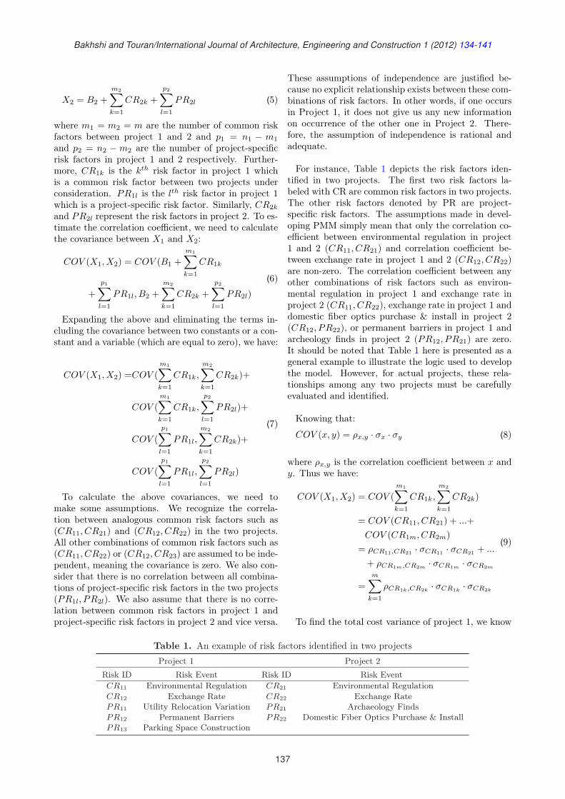
Bakhshi and Touran/International Journal of Architecture, Engineering and Construction 1 (2012) 134-141
X2 = B2 +m2∑
k=1
CR2k +p2∑
l=1
PR2l (5)
where m1 = m2 = m are the number of common riskfactors between project 1 and 2 and p1 = n1 − m1
and p2 = n2 − m2 are the number of project-specificrisk factors in project 1 and 2 respectively. Further-more, CR1k is the kth risk factor in project 1 whichis a common risk factor between two projects underconsideration. PR1l is the lth risk factor in project 1which is a project-specific risk factor. Similarly, CR2k
and PR2l represent the risk factors in project 2. To es-timate the correlation coefficient, we need to calculatethe covariance between X1 and X2:
COV (X1, X2) = COV (B1 +m1∑
k=1
CR1k
+p1∑
l=1
PR1l, B2 +m2∑
k=1
CR2k +p2∑
l=1
PR2l)
(6)
Expanding the above and eliminating the terms in-cluding the covariance between two constants or a con-stant and a variable (which are equal to zero), we have:
COV (X1, X2) =COV (m1∑
k=1
CR1k,
m2∑
k=1
CR2k)+
COV (m1∑
k=1
CR1k,
p2∑
l=1
PR2l)+
COV (p1∑
l=1
PR1l,
m2∑
k=1
CR2k)+
COV (p1∑
l=1
PR1l,
p2∑
l=1
PR2l)
(7)
To calculate the above covariances, we need tomake some assumptions. We recognize the correla-tion between analogous common risk factors such as(CR11, CR21) and (CR12, CR22) in the two projects.All other combinations of common risk factors such as(CR11, CR22) or (CR12, CR23) are assumed to be inde-pendent, meaning the covariance is zero. We also con-sider that there is no correlation between all combina-tions of project-specific risk factors in the two projects(PR1l, PR2l). We also assume that there is no corre-lation between common risk factors in project 1 andproject-specific risk factors in project 2 and vice versa.
These assumptions of independence are justified be-cause no explicit relationship exists between these com-binations of risk factors. In other words, if one occursin Project 1, it does not give us any new informationon occurrence of the other one in Project 2. There-fore, the assumption of independence is rational andadequate.
For instance, Table 1 depicts the risk factors iden-tified in two projects. The first two risk factors la-beled with CR are common risk factors in two projects.The other risk factors denoted by PR are project-specific risk factors. The assumptions made in devel-oping PMM simply mean that only the correlation co-efficient between environmental regulation in project1 and 2 (CR11, CR21) and correlation coefficient be-tween exchange rate in project 1 and 2 (CR12, CR22)are non-zero. The correlation coefficient between anyother combinations of risk factors such as environ-mental regulation in project 1 and exchange rate inproject 2 (CR11, CR22), exchange rate in project 1 anddomestic fiber optics purchase & install in project 2(CR12, PR22), or permanent barriers in project 1 andarcheology finds in project 2 (PR12, PR21) are zero.It should be noted that Table 1 here is presented as ageneral example to illustrate the logic used to developthe model. However, for actual projects, these rela-tionships among any two projects must be carefullyevaluated and identified.
Knowing that:
COV (x, y) = ρx,y · σx · σy (8)
where ρx,y is the correlation coefficient between x andy. Thus we have:
COV (X1, X2) = COV (m1∑
k=1
CR1k,
m2∑
k=1
CR2k)
= COV (CR11, CR21) + ...+COV (CR1m, CR2m)
= ρCR11,CR21 · σCR11 · σCR21 + ...
+ ρCR1m,CR2m · σCR1m · σCR2m
=m∑
k=1
ρCR1k,CR2k· σCR1k
· σCR2k
(9)
To find the total cost variance of project 1, we know
Table 1. An example of risk factors identified in two projects
Project 1 Project 2
Risk ID Risk Event Risk ID Risk EventCR11 Environmental Regulation CR21 Environmental RegulationCR12 Exchange Rate CR22 Exchange RatePR11 Utility Relocation Variation PR21 Archaeology FindsPR12 Permanent Barriers PR22 Domestic Fiber Optics Purchase & InstallPR13 Parking Space Construction
137
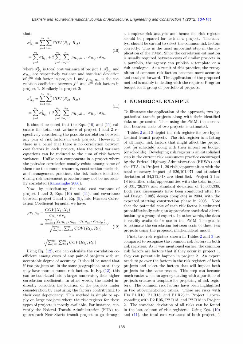
Bakhshi and Touran/International Journal of Architecture, Engineering and Construction 1 (2012) 134-141
that:
σ2X1
=n1∑
j=1
n1∑t=1
COV (R1j , R1t)
=n1∑
j=1
σ2R1j
+ 2n1∑
j=1
n1∑
t=j+1
ρR1j ,R1t· σR1j
· σR1t
(10)
where σ2X1
is total cost variance of project 1, σ2R1j
andσR1j
are respectively variance and standard deviationof jth risk factor in project 1, and ρR1j ,R1t
is the cor-relation coefficient between jth and tth risk factors inproject 1. Similarly in project 2:
σ2X2
=n2∑
j=1
n2∑t=1
COV (R2j , R2t)
=n2∑
j=1
σ2R2j
+ 2n2∑
j=1
n2∑
t=j+1
ρR2j ,R2t · σR2j · σR2t
(11)
It should be noted that the Eqs. (10) and (11) cal-culate the total cost variance of project 1 and 2 re-spectively considering the possible correlation betweenany pair of risk factors in each project. However, ifthere is a belief that there is no correlation betweencost factors in each project, then the total varianceequations can be reduced to the sum of risk factorsvariances. Unlike cost components in a project wherethe pairwise correlation usually exists among some ofthem due to common resources, construction methods,and management practices, the risk factors identifiedduring risk assessment procedure may not be necessar-ily correlated (Ranasinghe 2000).Now, by substituting the total cost variance of
project 1 and 2, Eqs. (10) and (11), and covariancebetween project 1 and 2, Eq. (9), into Pearson Corre-lation Coefficient formula, we have:
ρX1,X2 =COV (X1, X2)
σX1 · σX2
=∑m
k=1(ρCR1k,CR2k· σCR1k
· σCR2k)√∑n1
j=1
∑n1t=1 COV (R1j , R1t)
×
1√∑n2j=1
∑n2t=1 COV (R2j , R2t)
(12)
Using Eq. (12), one can calculate the correlation co-efficient among costs of any pair of projects with anacceptable degree of accuracy. It should be noted thatif two projects are in the same geographical area, theymay have more common risk factors. In Eq. (12), thiscan be translated into a larger numerator, thus highercorrelation coefficient. In other words, the model in-directly considers the location of the projects underconsideration by capturing the factors contributing totheir cost dependency. This method is simple to ap-ply on large projects where the risk register for thesetypes of projects is mostly available. For instance, cur-rently the Federal Transit Administration (FTA) re-quires each New Starts transit project to go through
a complete risk analysis and hence the risk registershould be prepared for each new project. The ana-lyst should be careful to select the common risk factorscorrectly. This is the most important step in the ap-plication of the PMM. Since the correlation estimationis usually required between costs of similar projects ina portfolio, the agency can publish a template or arisk catalogue. As a result of this practice, the recog-nition of common risk factors becomes more accurateand straight-forward. The application of the proposedmethod is mainly in dealing with the required Programbudget for a group or portfolio of projects.
4 NUMERICAL EXAMPLE
To illustrate the application of the approach, two hy-pothetical transit projects along with their identifiedrisks are presented. Then using the PMM, the correla-tion between costs of two projects is estimated.Tables 2 and 3 depict the risk register for two hypo-
thetical transit projects. The risk register is a listingof all major risk factors that might affect the projectcost (or schedule) along with their impact on budget(or schedule). Developing risk register is an establishedstep in the current risk assessment practice encouragedby the Federal Highway Administration (FHWA) andthe FTA. In Project 1, 26 risks/opportunities with thetotal monetary impact of $26,101,971 and standarddeviation of $4,212,318 are identified. Project 2 has18 identified risks/opportunities with the total impactof $31,726,377 and standard deviation of $5,033,338.Both risk assessments have been conducted after Fi-nal Design (100% design complete) in 2004, with theexpected starting construction phase in 2005. Notethat the potential cost of each risk factor is estimatedprobabilistically using an appropriate statistical distri-bution by a group of experts. In other words, the datais readily available for use in the PMM. The goal isto estimate the correlation between costs of these twoprojects using the proposed mathematical model.First, two risk registers shown in Tables 2 and 3 are
compared to recognize the common risk factors in bothrisk registers. As it was mentioned earlier, the commonrisk factors are factors that if they occur in project 1,they can potentially happen in project 2. An expertneeds to go over the factors in the risk registers of bothprojects and select the factors that will impact bothprojects for the same reason. This step can becomemuch easier when an agency dealing with a portfolio ofprojects creates a template for preparing of risk regis-ters. The common risk factors have been highlightedin two abovementioned tables. These are risks withIDs P1.R10, P1.R15, and P1.R23 in Project 1 corre-sponding with P2.R05, P2.R13, and P2.R18 in Project2. The standard deviation of all risks can be foundin the last column of risk registers. Using Eqs. (10)and (11), the total cost variances of both projects 1
138
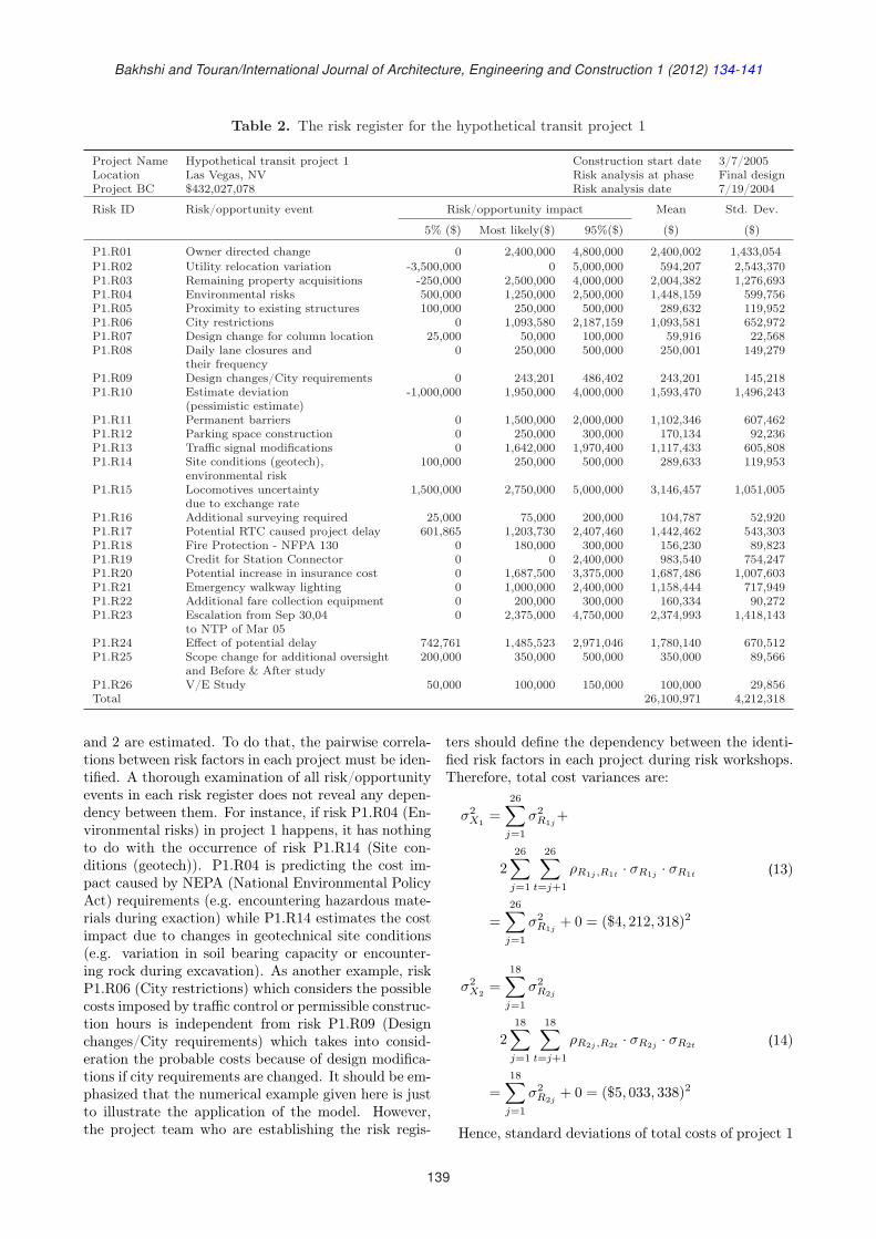
Bakhshi and Touran/International Journal of Architecture, Engineering and Construction 1 (2012) 134-141
Table 2. The risk register for the hypothetical transit project 1
Project Name Hypothetical transit project 1 Construction start date 3/7/2005Location Las Vegas, NV Risk analysis at phase Final designProject BC $432,027,078 Risk analysis date 7/19/2004
Risk ID Risk/opportunity event Risk/opportunity impact Mean Std. Dev.
5% ($) Most likely($) 95%($) ($) ($)
P1.R01 Owner directed change 0 2,400,000 4,800,000 2,400,002 1,433,054P1.R02 Utility relocation variation -3,500,000 0 5,000,000 594,207 2,543,370P1.R03 Remaining property acquisitions -250,000 2,500,000 4,000,000 2,004,382 1,276,693P1.R04 Environmental risks 500,000 1,250,000 2,500,000 1,448,159 599,756P1.R05 Proximity to existing structures 100,000 250,000 500,000 289,632 119,952P1.R06 City restrictions 0 1,093,580 2,187,159 1,093,581 652,972P1.R07 Design change for column location 25,000 50,000 100,000 59,916 22,568P1.R08 Daily lane closures and 0 250,000 500,000 250,001 149,279
their frequencyP1.R09 Design changes/City requirements 0 243,201 486,402 243,201 145,218P1.R10 Estimate deviation -1,000,000 1,950,000 4,000,000 1,593,470 1,496,243
(pessimistic estimate)P1.R11 Permanent barriers 0 1,500,000 2,000,000 1,102,346 607,462P1.R12 Parking space construction 0 250,000 300,000 170,134 92,236P1.R13 Traffic signal modifications 0 1,642,000 1,970,400 1,117,433 605,808P1.R14 Site conditions (geotech), 100,000 250,000 500,000 289,633 119,953
environmental riskP1.R15 Locomotives uncertainty 1,500,000 2,750,000 5,000,000 3,146,457 1,051,005
due to exchange rateP1.R16 Additional surveying required 25,000 75,000 200,000 104,787 52,920P1.R17 Potential RTC caused project delay 601,865 1,203,730 2,407,460 1,442,462 543,303P1.R18 Fire Protection - NFPA 130 0 180,000 300,000 156,230 89,823P1.R19 Credit for Station Connector 0 0 2,400,000 983,540 754,247P1.R20 Potential increase in insurance cost 0 1,687,500 3,375,000 1,687,486 1,007,603P1.R21 Emergency walkway lighting 0 1,000,000 2,400,000 1,158,444 717,949P1.R22 Additional fare collection equipment 0 200,000 300,000 160,334 90,272P1.R23 Escalation from Sep 30,04 0 2,375,000 4,750,000 2,374,993 1,418,143
to NTP of Mar 05P1.R24 Effect of potential delay 742,761 1,485,523 2,971,046 1,780,140 670,512P1.R25 Scope change for additional oversight 200,000 350,000 500,000 350,000 89,566
and Before & After studyP1.R26 V/E Study 50,000 100,000 150,000 100,000 29,856Total 26,100,971 4,212,318
and 2 are estimated. To do that, the pairwise correla-tions between risk factors in each project must be iden-tified. A thorough examination of all risk/opportunityevents in each risk register does not reveal any depen-dency between them. For instance, if risk P1.R04 (En-vironmental risks) in project 1 happens, it has nothingto do with the occurrence of risk P1.R14 (Site con-ditions (geotech)). P1.R04 is predicting the cost im-pact caused by NEPA (National Environmental PolicyAct) requirements (e.g. encountering hazardous mate-rials during exaction) while P1.R14 estimates the costimpact due to changes in geotechnical site conditions(e.g. variation in soil bearing capacity or encounter-ing rock during excavation). As another example, riskP1.R06 (City restrictions) which considers the possiblecosts imposed by traffic control or permissible construc-tion hours is independent from risk P1.R09 (Designchanges/City requirements) which takes into consid-eration the probable costs because of design modifica-tions if city requirements are changed. It should be em-phasized that the numerical example given here is justto illustrate the application of the model. However,the project team who are establishing the risk regis-
ters should define the dependency between the identi-fied risk factors in each project during risk workshops.Therefore, total cost variances are:
σ2X1
=26∑
j=1
σ2R1j
+
226∑
j=1
26∑
t=j+1
ρR1j ,R1t· σR1j
· σR1t
=26∑
j=1
σ2R1j
+ 0 = ($4, 212, 318)2
(13)
σ2X2
=18∑
j=1
σ2R2j
218∑
j=1
18∑
t=j+1
ρR2j ,R2t · σR2j · σR2t
=18∑
j=1
σ2R2j
+ 0 = ($5, 033, 338)2
(14)
Hence, standard deviations of total costs of project 1
139
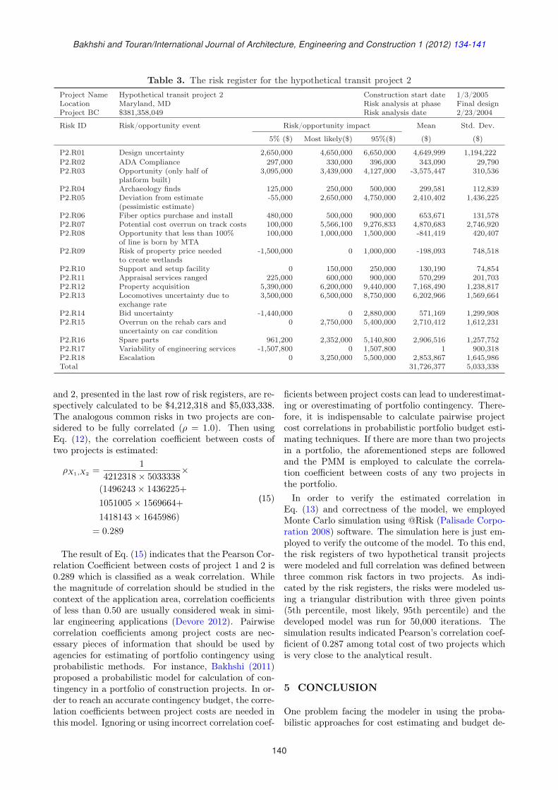
Bakhshi and Touran/International Journal of Architecture, Engineering and Construction 1 (2012) 134-141
Table 3. The risk register for the hypothetical transit project 2Project Name Hypothetical transit project 2 Construction start date 1/3/2005Location Maryland, MD Risk analysis at phase Final designProject BC $381,358,049 Risk analysis date 2/23/2004
Risk ID Risk/opportunity event Risk/opportunity impact Mean Std. Dev.
5% ($) Most likely($) 95%($) ($) ($)
P2.R01 Design uncertainty 2,650,000 4,650,000 6,650,000 4,649,999 1,194,222P2.R02 ADA Compliance 297,000 330,000 396,000 343,090 29,790P2.R03 Opportunity (only half of 3,095,000 3,439,000 4,127,000 -3,575,447 310,536
platform built)P2.R04 Archaeology finds 125,000 250,000 500,000 299,581 112,839P2.R05 Deviation from estimate -55,000 2,650,000 4,750,000 2,410,402 1,436,225
(pessimistic estimate)P2.R06 Fiber optics purchase and install 480,000 500,000 900,000 653,671 131,578P2.R07 Potential cost overrun on track costs 100,000 5,566,100 9,276,833 4,870,683 2,746,920P2.R08 Opportunity that less than 100% 100,000 1,000,000 1,500,000 -841,419 420,407
of line is born by MTAP2.R09 Risk of property price needed -1,500,000 0 1,000,000 -198,093 748,518
to create wetlandsP2.R10 Support and setup facility 0 150,000 250,000 130,190 74,854P2.R11 Appraisal services ranged 225,000 600,000 900,000 570,299 201,703P2.R12 Property acquisition 5,390,000 6,200,000 9,440,000 7,168,490 1,238,817P2.R13 Locomotives uncertainty due to 3,500,000 6,500,000 8,750,000 6,202,966 1,569,664
exchange rateP2.R14 Bid uncertainty -1,440,000 0 2,880,000 571,169 1,299,908P2.R15 Overrun on the rehab cars and 0 2,750,000 5,400,000 2,710,412 1,612,231
uncertainty on car conditionP2.R16 Spare parts 961,200 2,352,000 5,140,800 2,906,516 1,257,752P2.R17 Variability of engineering services -1,507,800 0 1,507,800 1 900,318P2.R18 Escalation 0 3,250,000 5,500,000 2,853,867 1,645,986Total 31,726,377 5,033,338
and 2, presented in the last row of risk registers, are re-spectively calculated to be $4,212,318 and $5,033,338.The analogous common risks in two projects are con-sidered to be fully correlated (ρ = 1.0). Then usingEq. (12), the correlation coefficient between costs oftwo projects is estimated:
ρX1,X2 =1
4212318× 5033338×
(1496243× 1436225+1051005× 1569664+1418143× 1645986)
= 0.289
(15)
The result of Eq. (15) indicates that the Pearson Cor-relation Coefficient between costs of project 1 and 2 is0.289 which is classified as a weak correlation. Whilethe magnitude of correlation should be studied in thecontext of the application area, correlation coefficientsof less than 0.50 are usually considered weak in simi-lar engineering applications (Devore 2012). Pairwisecorrelation coefficients among project costs are nec-essary pieces of information that should be used byagencies for estimating of portfolio contingency usingprobabilistic methods. For instance, Bakhshi (2011)proposed a probabilistic model for calculation of con-tingency in a portfolio of construction projects. In or-der to reach an accurate contingency budget, the corre-lation coefficients between project costs are needed inthis model. Ignoring or using incorrect correlation coef-
ficients between project costs can lead to underestimat-ing or overestimating of portfolio contingency. There-fore, it is indispensable to calculate pairwise projectcost correlations in probabilistic portfolio budget esti-mating techniques. If there are more than two projectsin a portfolio, the aforementioned steps are followedand the PMM is employed to calculate the correla-tion coefficient between costs of any two projects inthe portfolio.In order to verify the estimated correlation in
Eq. (13) and correctness of the model, we employedMonte Carlo simulation using @Risk (Palisade Corpo-ration 2008) software. The simulation here is just em-ployed to verify the outcome of the model. To this end,the risk registers of two hypothetical transit projectswere modeled and full correlation was defined betweenthree common risk factors in two projects. As indi-cated by the risk registers, the risks were modeled us-ing a triangular distribution with three given points(5th percentile, most likely, 95th percentile) and thedeveloped model was run for 50,000 iterations. Thesimulation results indicated Pearson’s correlation coef-ficient of 0.287 among total cost of two projects whichis very close to the analytical result.
5 CONCLUSION
One problem facing the modeler in using the proba-bilistic approaches for cost estimating and budget de-
140
Bakhshi and Touran/International Journal of Architecture, Engineering and Construction 1 (2012) 134-141
velopment for a project or a portfolio of projects is es-timating the correlation coefficient between cost com-ponents (i.e., cost items or project costs). In orderto reach a reasonable probabilistic cost estimate, therecognition of pairwise correlation between cost com-ponents is vital. Ignoring the dependency among costcomponents will result in underestimation of the to-tal cost variance. As was described, the most commonapproach is to provide subjective estimates of correla-tion coefficients. To the best of our knowledge, thereis no suggested method in literature for eliciting thecorrelation between costs of projects in a portfolio. Inthis paper, a new method, the PMM, was proposed toassist analysts systematically calculate the correlationcoefficient between costs of two projects where there isno historical data available. It should be noted thatthe objective of the method is to help an agency esti-mate the pairwise correlation among costs of any twoprojects in their portfolio. This is a necessary pieceof information to calculate portfolio contingency usingprobabilistic models.The PMM breaks down the cost of projects into a
base cost which is deterministic and risk costs whichcan be either deterministic or probabilistic. It is therisk costs that form the randomness of the total costand makes it possible to mathematically estimate thecorrelation between costs of two projects. Then, em-ploying the risk register of the projects, an expert iden-tifies the common risk factors among any two projects.Nowadays, for most of large projects the risk registeris developed in the early stages of project’s life. Inthose agencies that there is a template or risk cata-logue, identification of common risk factors becomeseasier and more accurate. Ultimately, a simple equa-tion is developed to estimate the correlation betweenproject costs using the standard deviations of identi-fied common risk factors. The proposed method can bean effective tool for agencies that utilize probabilisticcost estimating techniques for their portfolio of projectswhere the recognition of pairwise correlation amongproject costs results in more precise budget estimates.
REFERENCES
Bakhshi, P. (2011). A Bayesian Model for Control-ling Cost Overrun in a Portfolio of ConstructionProjects. PhD Dissertation, Northeastern University,Boston, Massachusetts, United States.
Chau, K. (1995). “Monte carlo simulation of construc-tion costs using subjective data.” Construction Man-agement and Economics, 13(5), 369–383.
Cho, S. (2006). “An exploratory project expert systemfor eliciting correlation coefficient and sequential up-dating of duration estimation.” Expert Systems withApplications, 30(4), 553–560.
Devore, J. L. (2012). Probability and Statistics forEngineering and the Sciences. Cengage Learning,Boston, Massachusetts, United States.
Iman, R. and Conover, W. (1982). “A distribution-freeapproach to inducing rank correlation among inputvariables.” Communications in Statistics-Simulationand Computation, 11(3), 311–334.
Iman, R. and Davenport, J. (1982). “Rank correlationplots for use with correlated input variables.” Com-munications in Statistics-Simulation and Computa-tion, 11(3), 335–360.
Ince, P. and Buongiono, J. (1991). “Multivariatestochastic simulation with subjective multivariatenormal distribution.” Symposium on System Analy-sis in Forest Resources, Charleston, South Carolina,United States.
Kurowicka, D. and Cooke, R. (2006). UncertaintyAnalysis with High Dimensional Dependence Mod-eling. Wiley, Hoboken, New Jersey, United States.
Palisade Corporation (2008). @Risk: Risk Analy-sis Add-in for Microsoft Excel. Ithaca, New York,United States.
Ranasinghe, M. (2000). “Impact of correlation and in-duced correlation on the estimation of project costof buildings.” Construction Management and Eco-nomics, 18(4), 395–406.
Ranasinghe, M. and Russel, A. (1992). “Treatment ofcorrelation for risk analysis of engineering projects.”Civil Engineering Systems, 9(1), 17–39.
Touran, A. (1993). “Probabilistic cost estimating withsubjective correlations.” Journal of Construction En-gineering and Management, 119(1), 58–71.
Touran, A. (2006). “Owners risk reduction techniquesusing a CM.” Construction Management Associationof America, Jones Branch Drive, McLean, Virginia,United States.
Touran, A. and Suphot, L. (1997). “Rank correlation insimulating construction costs.” Journal of Construc-tion Engineering and Management, 123(3), 297–301.
Touran, A. and Wiser, E. (1992). “Monte carlo tech-nique with correlated random variables.” Journal ofConstruction Engineering and Management, 118(2),258–272.
Wall, M. D. (1997). “Distributions and correlations inmonte carlo simulation.” Construction Managementand Economics, 15(3), 241–258.
Wang, W. (2002). “Simulation-facilitated model for as-sessing cost correlations.” Computer-Aided Civil andInfrastructure Engineering, 17(5), 368–380.
Wang, W. and Demsetz, L. (2000). “Model for evaluat-ing networks under correlated uncertainty-NETCO.”Journal of Construction Engineering and Manage-ment, 126(6), 458–466.
Yang, I. (2006). “Using gaussian copula to simulaterepetitive projects.” Construction Management andEconomics, 24(9), 901–909.
141
International Journal of Architecture, Engineering and ConstructionVol 1, No 3, September 2012, 142-154
Developing an Effective Bridge Facilities Management
Optimization Model
Xueqing Zhang∗
Department of Civil and Environmental Engineering, The Hong Kong University of Science and Technology,
Clear Water Bay, Kowloon, Hong Kong, China
Abstract: It is a great challenge to efficiently and effectively manage a bridge network of many differenttypes of bridges, which requires optimal allocation of limited resources to the right management actions in theright time in a long time horizon. This paper has developed a life-cycle performance-based bridge facilitiesmanagement methodology and the corresponding optimization model, which can (1) effectively measure andmodel the performance of the bridge network; (2) clearly define alternative management actions and effectivelymeasure their effectiveness in improving the performance of the network; (3) optimally plan short- and long-term works programs and distribute the limited resources among these programs; (4) effectively predict thelevel of performance of the bridge network as a result of the optimized distribution of resources, plan of works,and schedule of management actions; and (5) timely pre-warn the expected consequences due to inadequateresources. A hypothetical example is provided to demonstrate the use of the proposed life-cycle performance-based optimization model.
Keywords: Asset management, bridge facilities, condition index, deterioration, Markov decision process,optimization, performance, service life, stochastic process
DOI: 10.7492/IJAEC.2012.016
1 INTRODUCTION
In a country, region, province/state, or city, there isusually a number of bridges, which are hereinafter re-ferred to as the bridge network. Usually, it is the rele-vant (country, region, province/state, or city) govern-ment that is responsible for the operation and mainte-nance of this bridge network. To maintain the bridgenetwork at or above a certain required level of per-formance/serviceability, various management actionshave been taken to address a wide range of deterio-ration problems in the network. It is a great chal-lenge to manage the bridge network efficiently andcost-effectively over a long time horizon, given (1) thecomplexity of the bridge network (e.g., different types,sizes, ages, and functional requirements of bridges inthe network); (2) the wide range of risks and uncer-tainties (e.g., fluctuation of labor and material prices,material properties, construction quality, loading andusage, weather and other environmental conditions);(3) the different deterioration mechanisms of differentbridge components/elements over a long time horizon;and (4) the limited public financial budgets.
Efficient and cost-effective bridge facilities manage-ment requires optimal allocation of the limited re-sources to the right management actions in the righttime for all the bridges in the network and their com-ponents/elements such that the overall performanceof the network over a long time horizon is max-imized (Mori and Ellingwood 1993; Stewart 2001;Kong and Frangopol 2003; Robelin and Madanat 2007;Kobayashi et al. 2012; Zhang and Gao 2012). Here, thekey issue is how to determine the right management ac-tions for individual bridges, components and elementsat any time of a long time horizon from the point ofview of the bridge network. To deal with this issue,this paper has developed a life-cycle performance-basedbridge facilities management methodology and the cor-responding mathematical model, which are character-ized by the following five aspects:
1. The bridge network is hierarchically broken downwith each bridge decomposed into standardizedcomponents and elements, and the possible man-agement actions for each bridge elements are alsostandardized;
2. The bridge condition index (BCI) is used to mea-
*Email: [email protected]
142
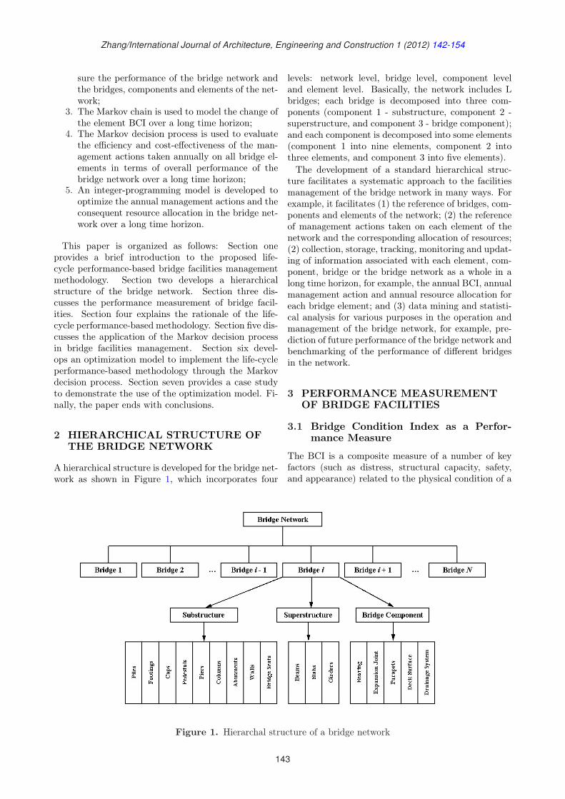
Zhang/International Journal of Architecture, Engineering and Construction 1 (2012) 142-154
sure the performance of the bridge network andthe bridges, components and elements of the net-work;
3. The Markov chain is used to model the change ofthe element BCI over a long time horizon;
4. The Markov decision process is used to evaluatethe efficiency and cost-effectiveness of the man-agement actions taken annually on all bridge el-ements in terms of overall performance of thebridge network over a long time horizon;
5. An integer-programming model is developed tooptimize the annual management actions and theconsequent resource allocation in the bridge net-work over a long time horizon.
This paper is organized as follows: Section oneprovides a brief introduction to the proposed life-cycle performance-based bridge facilities managementmethodology. Section two develops a hierarchicalstructure of the bridge network. Section three dis-cusses the performance measurement of bridge facil-ities. Section four explains the rationale of the life-cycle performance-based methodology. Section five dis-cusses the application of the Markov decision processin bridge facilities management. Section six devel-ops an optimization model to implement the life-cycleperformance-based methodology through the Markovdecision process. Section seven provides a case studyto demonstrate the use of the optimization model. Fi-nally, the paper ends with conclusions.
2 HIERARCHICAL STRUCTURE OFTHE BRIDGE NETWORK
A hierarchical structure is developed for the bridge net-work as shown in Figure 1, which incorporates four
levels: network level, bridge level, component leveland element level. Basically, the network includes Lbridges; each bridge is decomposed into three com-ponents (component 1 - substructure, component 2 -superstructure, and component 3 - bridge component);and each component is decomposed into some elements(component 1 into nine elements, component 2 intothree elements, and component 3 into five elements).The development of a standard hierarchical struc-
ture facilitates a systematic approach to the facilitiesmanagement of the bridge network in many ways. Forexample, it facilitates (1) the reference of bridges, com-ponents and elements of the network; (2) the referenceof management actions taken on each element of thenetwork and the corresponding allocation of resources;(2) collection, storage, tracking, monitoring and updat-ing of information associated with each element, com-ponent, bridge or the bridge network as a whole in along time horizon, for example, the annual BCI, annualmanagement action and annual resource allocation foreach bridge element; and (3) data mining and statisti-cal analysis for various purposes in the operation andmanagement of the bridge network, for example, pre-diction of future performance of the bridge network andbenchmarking of the performance of different bridgesin the network.
3 PERFORMANCE MEASUREMENTOF BRIDGE FACILITIES
3.1 Bridge Condition Index as a Perfor-mance Measure
The BCI is a composite measure of a number of keyfactors (such as distress, structural capacity, safety,and appearance) related to the physical condition of a
Figure 1. Hierarchal structure of a bridge network
143
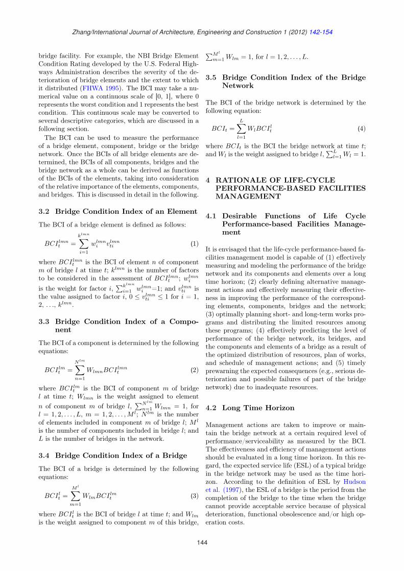
Zhang/International Journal of Architecture, Engineering and Construction 1 (2012) 142-154
bridge facility. For example, the NBI Bridge ElementCondition Rating developed by the U.S. Federal High-ways Administration describes the severity of the de-terioration of bridge elements and the extent to whichit distributed (FHWA 1995). The BCI may take a nu-merical value on a continuous scale of [0, 1], where 0represents the worst condition and 1 represents the bestcondition. This continuous scale may be converted toseveral descriptive categories, which are discussed in afollowing section.The BCI can be used to measure the performance
of a bridge element, component, bridge or the bridgenetwork. Once the BCIs of all bridge elements are de-termined, the BCIs of all components, bridges and thebridge network as a whole can be derived as functionsof the BCIs of the elements, taking into considerationof the relative importance of the elements, components,and bridges. This is discussed in detail in the following.
3.2 Bridge Condition Index of an Element
The BCI of a bridge element is defined as follows:
BCI lmnt =
klmn∑
i=1
wlmni vlmn
ti (1)
where BCI lmnt is the BCI of element n of component
m of bridge l at time t; klmn is the number of factorsto be considered in the assessment of BCI lmn
t ; wlmni
is the weight for factor i,∑klmn
i=1 wlmni =1; and vlmn
ti isthe value assigned to factor i, 0 ≤ vlmn
ti ≤ 1 for i = 1,2, . . ., klmn.
3.3 Bridge Condition Index of a Compo-nent
The BCI of a component is determined by the followingequations:
BCI lmt =
N lm∑n=1
WlmnBCI lmnt (2)
where BCI lmt is the BCI of component m of bridge
l at time t; Wlmn is the weight assigned to elementn of component m of bridge l,
∑N lm
n=1 Wlmn = 1, forl = 1, 2, . . . , L, m = 1, 2, . . . , M l; N lm is the numberof elements included in component m of bridge l; M l
is the number of components included in bridge l; andL is the number of bridges in the network.
3.4 Bridge Condition Index of a Bridge
The BCI of a bridge is determined by the followingequations:
BCI lt =
M l∑m=1
WlmBCI lmt (3)
where BCI lt is the BCI of bridge l at time t; and Wlm
is the weight assigned to component m of this bridge,
∑M l
m=1 Wlm = 1, for l = 1, 2, . . . , L.
3.5 Bridge Condition Index of the BridgeNetwork
The BCI of the bridge network is determined by thefollowing equation:
BCIt =L∑
l=1
WlBCI lt (4)
where BCIt is the BCI the bridge network at time t;and Wl is the weight assigned to bridge l,
∑Ll=1 Wl = 1.
4 RATIONALE OF LIFE-CYCLEPERFORMANCE-BASED FACILITIESMANAGEMENT
4.1 Desirable Functions of Life CyclePerformance-based Facilities Manage-ment
It is envisaged that the life-cycle performance-based fa-cilities management model is capable of (1) effectivelymeasuring and modeling the performance of the bridgenetwork and its components and elements over a longtime horizon; (2) clearly defining alternative manage-ment actions and effectively measuring their effective-ness in improving the performance of the correspond-ing elements, components, bridges and the network;(3) optimally planning short- and long-term works pro-grams and distributing the limited resources amongthese programs; (4) effectively predicting the level ofperformance of the bridge network, its bridges, andthe components and elements of a bridge as a result ofthe optimized distribution of resources, plan of works,and schedule of management actions; and (5) timelyprewarning the expected consequences (e.g., serious de-terioration and possible failures of part of the bridgenetwork) due to inadequate resources.
4.2 Long Time Horizon
Management actions are taken to improve or main-tain the bridge network at a certain required level ofperformance/serviceability as measured by the BCI.The effectiveness and efficiency of management actionsshould be evaluated in a long time horizon. In this re-gard, the expected service life (ESL) of a typical bridgein the bridge network may be used as the time hori-zon. According to the definition of ESL by Hudsonet al. (1997), the ESL of a bridge is the period from thecompletion of the bridge to the time when the bridgecannot provide acceptable service because of physicaldeterioration, functional obsolescence and/or high op-eration costs.
144
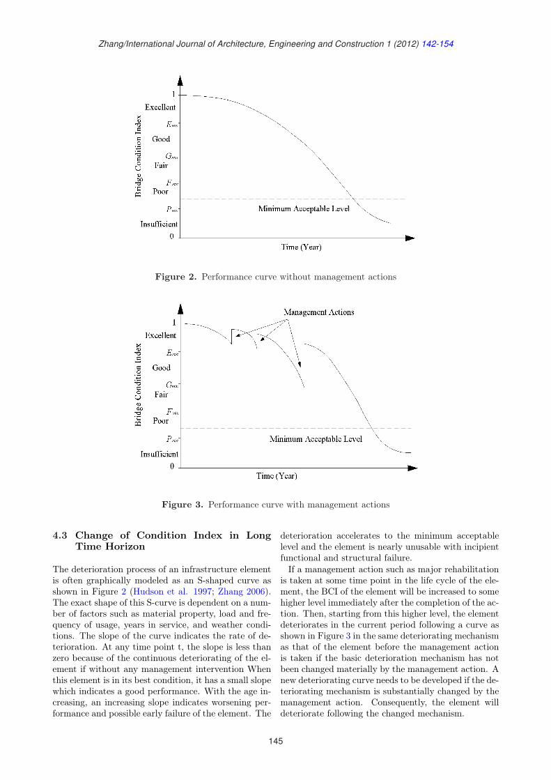
Zhang/International Journal of Architecture, Engineering and Construction 1 (2012) 142-154
Figure 2. Performance curve without management actions
Figure 3. Performance curve with management actions
4.3 Change of Condition Index in LongTime Horizon
The deterioration process of an infrastructure elementis often graphically modeled as an S-shaped curve asshown in Figure 2 (Hudson et al. 1997; Zhang 2006).The exact shape of this S-curve is dependent on a num-ber of factors such as material property, load and fre-quency of usage, years in service, and weather condi-tions. The slope of the curve indicates the rate of de-terioration. At any time point t, the slope is less thanzero because of the continuous deteriorating of the el-ement if without any management intervention Whenthis element is in its best condition, it has a small slopewhich indicates a good performance. With the age in-creasing, an increasing slope indicates worsening per-formance and possible early failure of the element. The
deterioration accelerates to the minimum acceptablelevel and the element is nearly unusable with incipientfunctional and structural failure.If a management action such as major rehabilitation
is taken at some time point in the life cycle of the ele-ment, the BCI of the element will be increased to somehigher level immediately after the completion of the ac-tion. Then, starting from this higher level, the elementdeteriorates in the current period following a curve asshown in Figure 3 in the same deteriorating mechanismas that of the element before the management actionis taken if the basic deterioration mechanism has notbeen changed materially by the management action. Anew deteriorating curve needs to be developed if the de-teriorating mechanism is substantially changed by themanagement action. Consequently, the element willdeteriorate following the changed mechanism.
145
Zhang/International Journal of Architecture, Engineering and Construction 1 (2012) 142-154
4.4 Stochastic Performance of Bridge Facil-ities
Figures 2 and 3 illustrate a deterministic approach tothe deterioration process and the change of BCI undermanagement actions. However, a wide range of factors(e.g., property of materials, construction quality, load-ing and usage of the bridge, and weather condition)affect the BCI of the element. There are substantialvariability and uncertainty of these factors, which havea combined effect on the BCI and render it to a stochas-tic variable:
1. The element may go to different conditions withvarying probabilities immediately after a man-agement action is taken; and
2. During the current period after a managementaction is taken, the element may deteriorate todifferent conditions with varying probabilities bythe end of the current period (the beginning ofthe following period).
4.5 Cost-Effectiveness of Management Ac-tions
The performance of any bridge element continuouslydeteriorates over time if no management action is takenon it. To maintain the element’s performance at orabove a certain level, management actions are neces-sary to improve the BCI of the element. This is alsotrue for the overall performance of the bridge networkas the performance of the network is a function of theperformance of all bridge elements.Different management actions have different effects
on the future performance of the element. For ex-ample, a routine maintenance action will make littleimprovement on the BCI of an element that is cur-rently in a poor condition whereas a replacement actionwill change the element to a completely new condition.Furthermore, different costs are required for differentmanagement actions on different bridge elements. Forthe same element, increasing costs are needed for rou-tine maintenance, minor rehabilitation, major rehabil-itation, and replacement. For the same managementaction, the cost is different one element from another.From previous discussion, it is known that the longer
the duration having a small slope is, the better theperformance of the element. Therefore, managementactions should be made in a cost-effective way suchthat the overall performance of the bridge network ismaximized over the planned long time horizon. This inessence requires that the limited budget be allocated tomanagement actions that maximize the marginal per-formance improvement of the bridge network per unitof budget spent. Generally, this requires that manage-ment actions be taken to avoid higher rate of deterio-ration over the planned long time horizon, taking intoconsideration of the relative importance of the bridges,components and elements.
5 BRIDGE FACILITIESMANAGEMENT THROUGHMARKOV DECISION PROCES
AMarkov decision process consists of five aspects (Put-erman 1994): decision epochs, states, actions, transi-tion probabilities and rewards, which are discussed inthe following in the context of bridge facilities manage-ment. Cesare et al. (1992) and Scherer and Glagola(1994) have proved the validity of the Markovian as-sumption in the bridge deterioration.
5.1 Decision Epochs and Periods
Decision epochs are the points of time when deci-sions are made. For the management of bridge fa-cilities, assume that decisions are made at the begin-ning of each year of the planned time horizon of Nyears, and let T denote the set of decision epochs, thenT = 1, 2, . . . , N.
5.2 State and Action Sets
At each decision epoch, each element occupies a state,the BCI of the element. Let Ω denote the set of pos-sible states for each element. Ω = [0, 1], which is acontinuous set of states, which may be converted to adescriptive and discrete state set Ω’= E, G, F , P , I,where E (excellent) = Emin ≤ BCI ≤ 1, Emin is theminimum numerical value of BCI that belongs to cat-egory E; G (good) = Gmin ≤ BCI < Emin, Gmin isthe minimum numerical value of BCI that belongs tocategory G; F (fair) = Fmin ≤ BCI < Gmin, Fmin isthe minimum numerical value of BCI that belongs tocategory F ; P (poor) = Pmin ≤ BCI < Fmin, Pmin isthe minimum numerical value of BCI that belongs tocategory P ; and I (insufficient) = 0 ≤ BCI < Pmin.At the beginning of year t, a management action a
is taken on an element that is at state It ∈ Ω. As-sume that there are always four standard actions (a1
= replacement, a2 = major rehabilitation, a3 = minorrehabilitation, and a4 = no action) no matter at whatstate an element is, then A = a1, a2, a3, a4 is the set ofmanagement actions. Ω and A do not vary with timet.
5.3 Rewards and Transition Probabilities
For any bridge element in state It ∈ Ω at the beginningof year t, if an action a ∈ A is taken, then there aretwo variables to measure the transition probabilities:
1. PItaIt, which measures the probability the ele-
ment BCI goes from state It to state Ita imme-diately after action a is taken; and
2. QIt+1Ita , which measures the probability the el-ement BCI goes from state Ita to state It+1
(It+1 ≤ Ita due to deterioration in year t) at thebeginning of year t+1 before any action is taken.
146
Zhang/International Journal of Architecture, Engineering and Construction 1 (2012) 142-154
A reward Rta is received as a result of taking actiona. This reward may be measured by the average per-formance of the element in year t as calculated in thefollowing equations:
Rta =12
∑
Ita∈Ω
PItaIt×
(Ita +∑
It+1∈Ω
QIt+1ItaIt+1)(5)
where∑
Ita∈Ω PItaIt = 1 and∑
It+1∈Ω QIt+1Ita = 1 fort = 1, 2, . . . , N , and a = 1, 2, 3 and 4.
6 LIFE CYCLEPERFORMANCE-BASEDOPTIMIZATION MODEL
Based on the ideas discussed in previous sections, aninteger-programming model based on the Markov de-cision process has been developed. The objective ofthe optimization model is to maximize the overall per-formance of the bridge network over the planned longtime horizon by optimizing the set of annual manage-ment actions on all bridge elements, subject to variousconstraints, such as annual budget and minimum per-formance requirements for the bridge network. Detailsof this model are presented in the following sections.
6.1 Decision Variable
Y atIlmn
tis a binary variable; Y a
tIlmnt
= 1 if action a istaken when element n of component m of bridge l iscurrently at a BCI of I lmn
t at the beginning of year t;Y a
tIlmnt
= 0 if action a is not taken; I lmnt = condition
index of element n of component m of bridge l at thebeginning of year t before any management action a istaken, and I lmn
t = 1 [excellent (E)], 2 [good (G)], 3[fair (E)], 4 [poor (P )] and 5 [insufficient (I)] ; a = anaction to be taken, and a = 1 (replacement), 2 (majorrehabilitation), 3 (minor rehabilitation), and 4 (routinemaintenance).
6.2 Objective Function
Max Zt =L∑
l=1
M l∑m=1
N lm∑n=1
4∑a=1
WlWlmWlmnY atIlmn
t
[5∑
Ilmnta =1
PIlmnta Ilmn
t×
(I lmnta +
5∑
Ilmnt+1 =1
QIlmnt+1 Ilmn
taI lmnt+1 )]
(6)
where Zt = weighted overall performance level of thebridge network in year t; I lmn
ta = condition index ofelement n of component m of bridge l at the beginningof year t immediately after a management action a istaken, when the element is at condition I lmn
t at the be-
ginning of year t before any action is taken; PIlmnta Ilmn
t
= probability of element n of component m of bridgel to go to condition I lmn
ta immediately after a manage-ment action a is taken when it is in condition I lmn
t atthe beginning of year t,
∑5Ilmn
ta =1 PIlmnta Ilmn
t= 1 for a
= 1, 2, 3, 4; and QIlmnt+1 Ilmn
ta= probability of element n
of component m of bridge l to go to condition I lmnt+1 at
the beginning of year t + 1 before any action is takenwhen it is in condition I lmn
ta at the beginning of year t,and
∑5Ilmn
t+1 =1 QIlmnt+1 Ilmn
tafor a = 1, 2, 3, 4.
6.3 Constraints
Budget Constraints
(1) Network Budget Constraint
L∑
l=1
M l∑m=1
N lm∑n=1
4∑a=1
CatIlmn
tY a
tIlmnt
≤ Bt (7)
where CatIlmn
t= cost corresponding to management ac-
tion a when element n of component m of bridge l isat condition I lmn
t in the beginning of year t; and Bt
is the total budget available for the bridge network inyear t.
(2) Bridge Budget Constraints
M l∑m=1
N lm∑n=1
4∑a=1
CatIlmn
tY a
tIlmnt
≤ Blt
for l = 1, 2, . . . , L
(8)
where Blt is the maximum amount of budget that can
be used for bridge l in year t.
Minimum Acceptable Performance Constraints
Minimum performance levels may be required forthe bridge network, individual bridges, componentsand elements, depending on their relative importance,health, safety and environment requirements, and theeconomics.
(1) Minimum Element Performance Requirement
12
4∑a=1
5∑
Ilmnta =1
[PIlmnta Ilmn
t(I lmn
ta +
5∑
Ilmnt+1 =1
QIlmnt+1 Ilmn
taI lmnt+1 )Y a
tIlmnt
] ≥ BCIlmn
for l = 1, 2, . . . , L,m = 1, 2, . . . , M l,
n = 1, 2, . . . , N lm
(9)
where BCIlmn is the required minimum level of per-formance for element n of component m of bridge l.
147
Zhang/International Journal of Architecture, Engineering and Construction 1 (2012) 142-154
(2) Minimum Year-end Element BCI Requirement4∑
a=1
5∑
Ilmnta =1
[(PIlmnta Ilmn
t
5∑
Ilmnt+1 =1
QIlmnt+1 Ilmn
taI lmnt+1 )
Y atIlmn
t] ≥ BCIend
lmn
for l = 1, 2, . . . , L, m = 1, 2, . . . , M l,
n = 1, 2, . . . , N lm
(10)
where BCIendlmn is the required minimum element BCI
at the end of the year before any management actionis taken.
(3) Minimum Component Performance Requirement
12
N lm∑n=1
4∑a=1
5∑
Ilmnta =1
[WlmnPIlmnta Ilmn
t(I lmn
ta +
5∑
Ilmnt+1 =1
QIlmnt+1 Ilmn
taI lmnt+1 )Y a
tIlmnt
] ≥ BCIlm
for l = 1, 2, . . . , L, m = 1, 2, . . . , M l,
(11)
where BCIlm is the required minimum level of perfor-mance for component m of bridge l.
(4) Minimum Bridge Performance Requirement
12
M l∑m=1
N lm∑n=1
4∑a=1
5∑
Ilmnta =1
[WlmWlmnPIlmnta Ilmn
t
(I lmnta +
5∑
Ilmnt+1 =1
QIlmnt+1 Ilmn
taI lmnt+1 )Y a
tIlmnt
] ≥ BCIl
for l = 1, 2, . . . , L
(12)
where BCIl is the required minimum performance levelfor bridge l.
(5) Minimum Bridge Network Performance Require-ment
12
L∑
l=1
M l∑m=1
N lm∑n=1
4∑a=1
5∑
Ilmnta =1
[WlWlmWlmnPIlmnta Ilmn
t(I lmn
ta +5∑
Ilmnt+1 =1
QIlmnt+1 Ilmn
taI lmnt+1 )Y a
tIlmnt
] ≥ BCI
(13)
where BCI is the required minimum performance levelfor the bridge network.
Only One Action Actually Taken for an Element
4∑a=1
Y atIlmn
t= 1
for l = 1, 2, . . . , L,m = 1, 2, . . . , M l,
n = 1, 2, . . . , N lm, and I lmnt = 1, 2, 3, 4, 5
(14)
Binary Constraints
Y atIlmn
t= 0, 1
for l = 1, 2, . . . , L,m = 1, 2, . . . , M l,
n = 1, 2, . . . , N lm, I lmnt = 1, 2, 3, 4, 5,
and a = 1, 2, 3, 4
(15)
7 CASE STUDY
A case study of a hypothetical bridge network thatincludes two bridges (1 and 2) is conducted todemonstrate the application of the proposed life-cycleperformance-based optimization model for bridge facil-ities management. For simplicity and convenience, inthe breakdown of the bridge network, the componentor element number is used to represent the correspond-ing component or element instead of using the name ofthe component or element. Please note that the inputdata used in this case study are hypothetical and maynot reflect the reality.
7.1 Life-Cycle Performance-Based Opti-mization Model
Objective Function
For simplicity, assume that (1) the weights of 0.4 and0.6 are used for bridges 1 and 2 respectively to reflecttheir relative importance; (2) the three components ofbridge 1 or 2 are equally important; and (3) the ele-ments in each of the three components of bridge 1 or 2are equally important, then the objective function canbe expressed as follows:
Max Zt =0.43∑
m=1
N1m∑n=1
4∑a=1
13W1mnY a
tI1mnt
×
[5∑
I1mnta =1
PI1mnta I1mn
t(I1mn
ta +
5∑
I1mnt+1 =1
QI1mnt+1 I1mn
taI1mnt+1 )]+
0.63∑
m=1
N2m∑n=1
4∑a=1
13W2mnY a
tI2mnt
×
[5∑
I2mnta =1
PI2mnta I21n
t(I2mn
ta +
5∑
I2mnt+1 =1
QI2mnt+1 I2mn
taI2mnt+1 )]
(16)
where N lm = 9, Wlmn = 1/9 if m = 1; N lm =3, Wlmn = 1/3 if m = 2; and N lm = 5, Wlmn = 1/9 ifm = 3, for l = 1, 2.
148
Zhang/International Journal of Architecture, Engineering and Construction 1 (2012) 142-154
Network Budget Constraint
Assume that the total budget available for the bridgenetwork is $1,000,000 per year, then
9∑n=1
4∑a=1
CatI11n
tY a
tI11nt
+3∑
n=1
4∑a=1
CatI12n
tY a
tI12nt
+
5∑n=1
4∑a=1
CatI13n
tY a
tI13nt
+9∑
n=1
4∑a=1
CatI21n
tY a
tI21nt
+
3∑n=1
4∑a=1
CatI22n
tY a
tI22nt
+5∑
n=1
4∑a=1
CatI23n
tY a
tI23nt
≤ Bt
(17)
Minimum Element Performance Requirement
Assume that the minimum required level of perfor-mance for any bridge element is 0.3, which is the meanvalue of BCI in the category of P (poor), then
12
4∑a=1
5∑
Ilmnta =1
[PIlmnta Ilmn
t(I lmn
ta +
5∑
Ilmnt+1 =1
QIlmnt+1 Ilmn
taI lmnt+1 )Y a
tIlmnt
] ≥ 0.3
for l = 1, 2; m = 1, 2, 3; n = 1, . . . , 9 if m = 1;n = 1, 2, 3 if m = 2; n = 1, 2, 3, 4, 5 if m = 3
(18)
Minimum Year-end Element BCI Requirement
Assume that the minimum required BCI for any bridgeelement at the end of the current year before any man-agement action is taken is 0.3, which is the mean valueof BCI in the category of P (poor), then
4∑a=1
5∑
Ilmnta =1
[(PIlmnta Ilmn
t
5∑
Ilmnt+1 =1
QIlmnt+1 Ilmn
taI lmnt+1 )
Y atIlmn
t] ≥ 0.3
for l = 1, 2; m = 1, 2, 3; n = 1, . . . , 9 if m = 1;n = 1, 2, 3 if m = 2; n = 1, 2, 3, 4, 5 if m = 3
(19)
Minimum Component Performance Requirement
Assume that the minimum required level of perfor-mance for any bridge component is 0.5, which is themean value of BCI in the category of F (fair), then
12
N lm∑n=1
4∑a=1
5∑
Ilmnta =1
[WlmnPIlmnta Ilmn
t(I lmn
ta +
5∑
Ilmnt+1 =1
QIlmnt+1 Ilmn
taI lmnt+1 )Y a
tIlmnt
] ≥ 0.5
for l = 1, 2; m = 1, 2, 3
(20)
Minimum Bridge Performance Requirement
Assume that the minimum required level of perfor-mance for any bridge is 0.6, which is the minimumvalue of BCI in the category of G (good), then
12
3∑m=1
N lm∑n=1
4∑a=1
5∑
Ilmnta =1
[13WlmnPIlmn
ta Ilmnt
(I lmnta +
5∑
Ilmnt+1 =1
QIlmnt+1 Ilmn
taI lmnt+1 )Y a
tIlmnt
] ≥ 0.6
for l = 1, 2
(21)
Minimum Network Performance Requirement
Assume that the minimum required level of perfor-mance for the bridge network is 0.6, which is the min-imum value of BCI in the category of G (good), then
12
3∑m=1
N1m∑n=1
4∑a=1
5∑
I1mnta =1
[0.413W1mnPI1mn
ta I1mnt
(I1mnta +
5∑
I1mnt+1 =1
QI1mnt+1 I1mn
taI1mnt+1 )Y a
tI1mnt
]+
3∑m=1
N2m∑n=1
4∑a=1
5∑
I2mnta =1
[0.613W2mnPI2mn
ta I2mnt
(I2mnta +
5∑
I2mnt+1 =1
QI2mnt+1 I2mn
taI2mnt+1 )Y a
tI2mnt
] ≥ 0.6
(22)
Table 1. Element condition index at the beginning of year t
Element Component 1 Component 2 Component 3
1 2 3 4 5 6 7 8 9 1 2 3 1 2 3 4 5Bridge 1
Descriptive category G G E E F F P G I G F F E G F P PNumerical value 0.7 0.7 0.9 0.9 0.5 0.5 0.3 0.7 0.1 0.7 0.5 0.5 0.9 0.7 0.5 0.3 0.3
Bridge 2Descriptive category E G E F G P I F G G F G G F E I PNumerical value 0.9 0.7 0.9 0.5 0.7 0.3 0.1 0.5 0.7 0.7 0.5 0.7 0.7 0.5 0.9 0.1 0.3
149
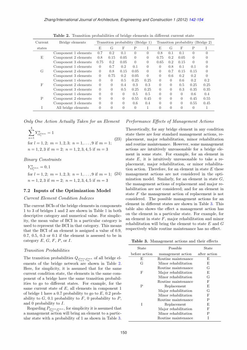
Zhang/International Journal of Architecture, Engineering and Construction 1 (2012) 142-154
Table 2. Transition probabilities of bridge elements in different current state
Current Bridge elements Transition probability (Bridge 1) Transition probability (Bridge 2)states E G F P I E G F P I
Component 1 elements 0.7 0.2 0.1 0 0 0.8 0.1 0.1 0 0E Component 2 elements 0.8 0.15 0.05 0 0 0.75 0.2 0.05 0 0
Component 3 elements 0.75 0.2 0.05 0 0 0.65 0.2 0.15 0 0Component 1 elements 0 0.7 0.2 0.1 0 0 0.8 0.1 0.1 0
G Component 2 elements 0 0.8 0.15 0.05 0 0 0.7 0.15 0.15 0Component 3 elements 0 0.75 0.2 0.05 0 0 0.6 0.2 0.2 0Component 1 elements 0 0 0.5 0.25 0.25 0 0 0.6 0.2 0.2
F Component 2 elements 0 0 0.4 0.3 0.3 0 0 0.5 0.25 0.25Component 3 elements 0 0 0.5 0.25 0.25 0 0 0.3 0.35 0.35Component 1 elements 0 0 0 0.5 0.5 0 0 0 0.6 0.4
P Component 2 elements 0 0 0 0.55 0.45 0 0 0 0.45 0.55Component 3 elements 0 0 0 0.6 0.4 0 0 0 0.55 0.45
I All bridge elements 0 0 0 0 1 0 0 0 0 1
Only One Action Actually Taken for an Element4∑
a=1
Y atIlmn
t= 1
for l = 1, 2; m = 1, 2, 3; n = 1, . . . , 9 if m = 1;n = 1, 2, 3 if m = 2; n = 1, 2, 3, 4, 5 if m = 3
(23)
Binary Constraints
Y atIlmn
t= 0, 1
for l = 1, 2; m = 1, 2, 3; n = 1, . . . , 9 if m = 1;n = 1, 2, 3 if m = 2; n = 1, 2, 3, 4, 5 if m = 3
(24)
7.2 Inputs of the Optimization Model
Current Element Condition Indexes
The current BCIs of the bridge elements in components1 to 3 of bridges 1 and 2 are shown in Table 1 in bothdescriptive category and numerical value. For simplic-ity, the mean value of BCI in a particular category isused to represent the BCI in that category. This meansthat the BCI of an element is assigned a value of 0.9,0.7, 0.5, 0.3 or 0.1 if the element is assessed to be incategory E, G, F , P , or I.
Transition Probabilities
The transition probabilities QIlmnt+1 Ilmn
taof all bridge el-
ements of the bridge network are shown in Table 2.Here, for simplicity, it is assumed that for the samecurrent condition state, the elements in the same com-ponent of a bridge have the same transition probabil-ities to go to different states. For example, for thesame current state of E, all elements in component 1of bridge 1 have a 0.7 probability to go to E, 0.2 prob-ability to G, 0.1 probability to F , 0 probability to P ,and 0 probability to I.Regarding PIlmn
ta Ilmnt
, for simplicity it is assumed thata management action will bring an element to a partic-ular state with a probability of 1 as shown in Table 3.
Performance Effects of Management Actions
Theoretically, for any bridge element in any conditionstate there are four standard management actions, re-placement, major rehabilitation, minor rehabilitationand routine maintenance. However, some managementactions are intuitively unreasonable for a bridge ele-ment in some state. For example, for an element instate E, it is intuitively unreasonable to take a re-placement, major rehabilitation, or minor rehabilita-tion action. Therefore, for an element in state E thesemanagement actions are not considered in the opti-mization model. Similarly, for an element in state G,the management actions of replacement and major re-habilitation are not considered; and for an element instate F the management action of replacement is notconsidered. The possible management actions for anelement in different states are shown in Table 3. Thistable also shows the effect a management action hason the element in a particular state. For example, foran element in state F , major rehabilitation and minorrehabilitation will bring the element to state E and Grespectively while routine maintenance has no effect.
Table 3. Management actions and their effects
State Possible Statebefore action management action after action
E Routine maintenance EG Minor rehabilitation E
Routine maintenance GF Major rehabilitation E
Minor rehabilitation GRoutine maintenance F
P Replacement EMajor rehabilitation GMinor rehabilitation FRoutine maintenance P
I Replacement EMajor rehabilitation FMinor rehabilitation PRoutine maintenance I
150
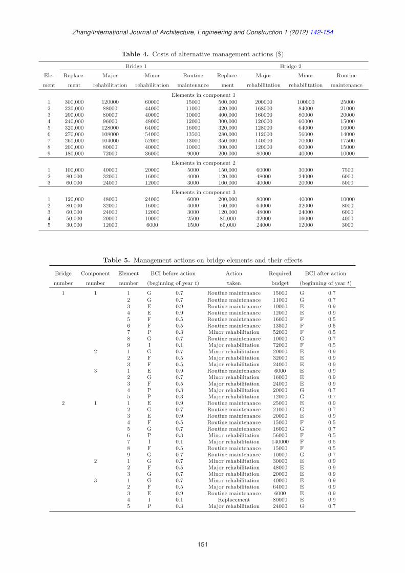
Zhang/International Journal of Architecture, Engineering and Construction 1 (2012) 142-154
Table 4. Costs of alternative management actions ($)
Bridge 1 Bridge 2
Ele- Replace- Major Minor Routine Replace- Major Minor Routine
ment ment rehabilitation rehabilitation maintenance ment rehabilitation rehabilitation maintenance
Elements in component 11 300,000 120000 60000 15000 500,000 200000 100000 250002 220,000 88000 44000 11000 420,000 168000 84000 210003 200,000 80000 40000 10000 400,000 160000 80000 200004 240,000 96000 48000 12000 300,000 120000 60000 150005 320,000 128000 64000 16000 320,000 128000 64000 160006 270,000 108000 54000 13500 280,000 112000 56000 140007 260,000 104000 52000 13000 350,000 140000 70000 175008 200,000 80000 40000 10000 300,000 120000 60000 150009 180,000 72000 36000 9000 200,000 80000 40000 10000
Elements in component 21 100,000 40000 20000 5000 150,000 60000 30000 75002 80,000 32000 16000 4000 120,000 48000 24000 60003 60,000 24000 12000 3000 100,000 40000 20000 5000
Elements in component 31 120,000 48000 24000 6000 200,000 80000 40000 100002 80,000 32000 16000 4000 160,000 64000 32000 80003 60,000 24000 12000 3000 120,000 48000 24000 60004 50,000 20000 10000 2500 80,000 32000 16000 40005 30,000 12000 6000 1500 60,000 24000 12000 3000
Table 5. Management actions on bridge elements and their effects
Bridge Component Element BCI before action Action Required BCI after action
number number number (beginning of year t) taken budget (beginning of year t)
1 1 1 G 0.7 Routine maintenance 15000 G 0.72 G 0.7 Routine maintenance 11000 G 0.73 E 0.9 Routine maintenance 10000 E 0.94 E 0.9 Routine maintenance 12000 E 0.95 F 0.5 Routine maintenance 16000 F 0.56 F 0.5 Routine maintenance 13500 F 0.57 P 0.3 Minor rehabilitation 52000 F 0.58 G 0.7 Routine maintenance 10000 G 0.79 I 0.1 Major rehabilitation 72000 F 0.5
2 1 G 0.7 Minor rehabilitation 20000 E 0.92 F 0.5 Major rehabilitation 32000 E 0.93 F 0.5 Major rehabilitation 24000 E 0.9
3 1 E 0.9 Routine maintenance 6000 E 0.92 G 0.7 Minor rehabilitation 16000 E 0.93 F 0.5 Major rehabilitation 24000 E 0.94 P 0.3 Major rehabilitation 20000 G 0.75 P 0.3 Major rehabilitation 12000 G 0.7
2 1 1 E 0.9 Routine maintenance 25000 E 0.92 G 0.7 Routine maintenance 21000 G 0.73 E 0.9 Routine maintenance 20000 E 0.94 F 0.5 Routine maintenance 15000 F 0.55 G 0.7 Routine maintenance 16000 G 0.76 P 0.3 Minor rehabilitation 56000 F 0.57 I 0.1 Major rehabilitation 140000 F 0.58 F 0.5 Routine maintenance 15000 F 0.59 G 0.7 Routine maintenance 10000 G 0.7
2 1 G 0.7 Minor rehabilitation 30000 E 0.92 F 0.5 Major rehabilitation 48000 E 0.93 G 0.7 Minor rehabilitation 20000 E 0.9
3 1 G 0.7 Minor rehabilitation 40000 E 0.92 F 0.5 Major rehabilitation 64000 E 0.93 E 0.9 Routine maintenance 6000 E 0.94 I 0.1 Replacement 80000 E 0.95 P 0.3 Major rehabilitation 24000 G 0.7
151
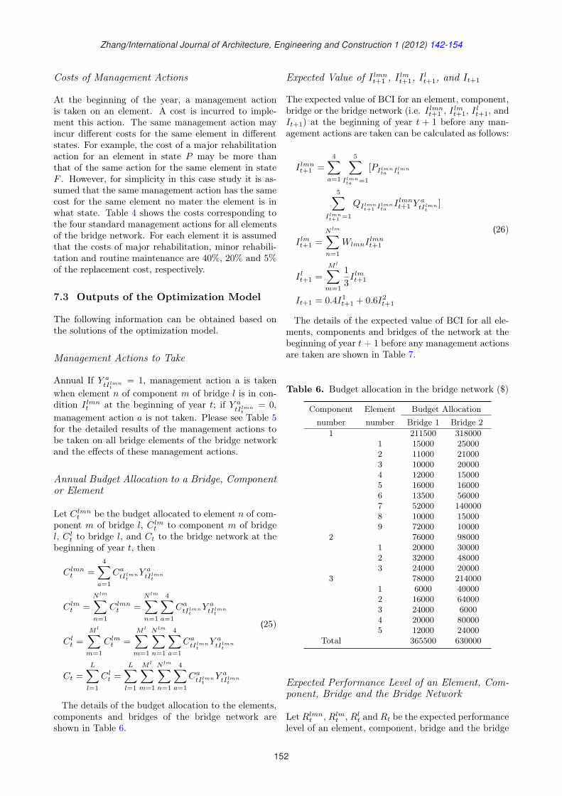
Zhang/International Journal of Architecture, Engineering and Construction 1 (2012) 142-154
Costs of Management Actions
At the beginning of the year, a management actionis taken on an element. A cost is incurred to imple-ment this action. The same management action mayincur different costs for the same element in differentstates. For example, the cost of a major rehabilitationaction for an element in state P may be more thanthat of the same action for the same element in stateF . However, for simplicity in this case study it is as-sumed that the same management action has the samecost for the same element no mater the element is inwhat state. Table 4 shows the costs corresponding tothe four standard management actions for all elementsof the bridge network. For each element it is assumedthat the costs of major rehabilitation, minor rehabili-tation and routine maintenance are 40%, 20% and 5%of the replacement cost, respectively.
7.3 Outputs of the Optimization Model
The following information can be obtained based onthe solutions of the optimization model.
Management Actions to Take
Annual If Y atIlmn
t= 1, management action a is taken
when element n of component m of bridge l is in con-dition I lmn
t at the beginning of year t; if Y atIlmn
t= 0,
management action a is not taken. Please see Table 5for the detailed results of the management actions tobe taken on all bridge elements of the bridge networkand the effects of these management actions.
Annual Budget Allocation to a Bridge, Componentor Element
Let Clmnt be the budget allocated to element n of com-
ponent m of bridge l, Clmt to component m of bridge
l, Clt to bridge l, and Ct to the bridge network at the
beginning of year t, then
Clmnt =
4∑a=1
CatIlmn
tY a
tIlmnt
Clmt =
N lm∑n=1
Clmnt =
N lm∑n=1
4∑a=1
CatIlmn
tY a
tIlmnt
Clt =
M l∑m=1
Clmt =
M l∑m=1
N lm∑n=1
4∑a=1
CatIlmn
tY a
tIlmnt
Ct =L∑
l=1
Clt =
L∑
l=1
M l∑m=1
N lm∑n=1
4∑a=1
CatIlmn
tY a
tIlmnt
(25)
The details of the budget allocation to the elements,components and bridges of the bridge network areshown in Table 6.
Expected Value of I lmnt+1 , I lm
t+1, I lt+1, and It+1
The expected value of BCI for an element, component,bridge or the bridge network (i.e. I lmn
t+1 , I lmt+1, I l
t+1, andIt+1) at the beginning of year t + 1 before any man-agement actions are taken can be calculated as follows:
I lmnt+1 =
4∑a=1
5∑
Ilmnta =1
[PIlmnta Ilmn
t
5∑
Ilmnt+1 =1
QIlmnt+1 Ilmn
taI lmnt+1 Y a
tIlmnt
]
I lmt+1 =
N lm∑n=1
WlmnI lmnt+1
I lt+1 =
M l∑m=1
13I lmt+1
It+1 = 0.4I1t+1 + 0.6I2
t+1
(26)
The details of the expected value of BCI for all ele-ments, components and bridges of the network at thebeginning of year t + 1 before any management actionsare taken are shown in Table 7.
Table 6. Budget allocation in the bridge network ($)
Component Element Budget Allocationnumber number Bridge 1 Bridge 2
1 211500 3180001 15000 250002 11000 210003 10000 200004 12000 150005 16000 160006 13500 560007 52000 1400008 10000 150009 72000 10000
2 76000 980001 20000 300002 32000 480003 24000 20000
3 78000 2140001 6000 400002 16000 640003 24000 60004 20000 800005 12000 24000
Total 365500 630000
Expected Performance Level of an Element, Com-ponent, Bridge and the Bridge Network
Let Rlmnt , Rlm
t , Rlt and Rt be the expected performance
level of an element, component, bridge and the bridge
152
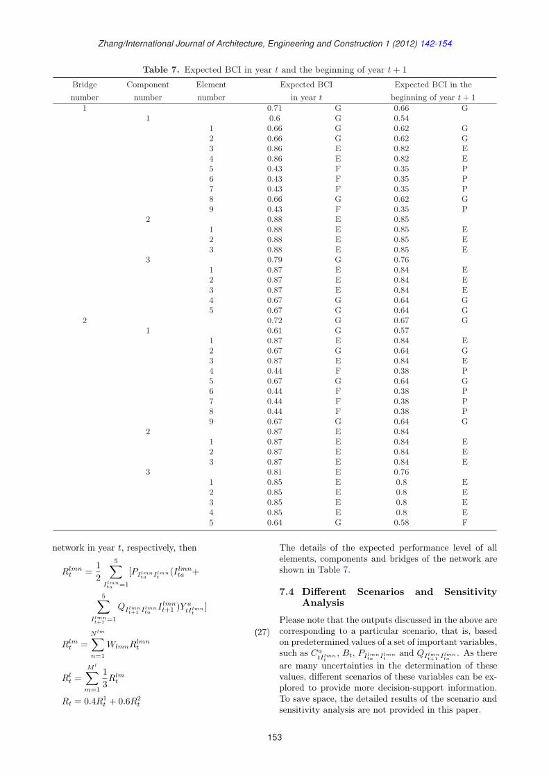
Zhang/International Journal of Architecture, Engineering and Construction 1 (2012) 142-154
Table 7. Expected BCI in year t and the beginning of year t + 1
Bridge Component Element Expected BCI Expected BCI in thenumber number number in year t beginning of year t + 1
1 0.71 G 0.66 G1 0.6 G 0.54
1 0.66 G 0.62 G2 0.66 G 0.62 G3 0.86 E 0.82 E4 0.86 E 0.82 E5 0.43 F 0.35 P6 0.43 F 0.35 P7 0.43 F 0.35 P8 0.66 G 0.62 G9 0.43 F 0.35 P
2 0.88 E 0.851 0.88 E 0.85 E2 0.88 E 0.85 E3 0.88 E 0.85 E
3 0.79 G 0.761 0.87 E 0.84 E2 0.87 E 0.84 E3 0.87 E 0.84 E4 0.67 G 0.64 G5 0.67 G 0.64 G
2 0.72 G 0.67 G1 0.61 G 0.57
1 0.87 E 0.84 E2 0.67 G 0.64 G3 0.87 E 0.84 E4 0.44 F 0.38 P5 0.67 G 0.64 G6 0.44 F 0.38 P7 0.44 F 0.38 P8 0.44 F 0.38 P9 0.67 G 0.64 G
2 0.87 E 0.841 0.87 E 0.84 E2 0.87 E 0.84 E3 0.87 E 0.84 E
3 0.81 E 0.761 0.85 E 0.8 E2 0.85 E 0.8 E3 0.85 E 0.8 E4 0.85 E 0.8 E5 0.64 G 0.58 F
network in year t, respectively, then
Rlmnt =
12
5∑
Ilmnta =1
[PIlmnta Ilmn
t(I lmn
ta +
5∑
Ilmnt+1 =1
QIlmnt+1 Ilmn
taI lmnt+1 )Y a
tIlmnt
]
Rlmt =
N lm∑n=1
WlmnRlmnt
Rlt =
M l∑m=1
13Rlm
t
Rt = 0.4R1t + 0.6R2
t
(27)
The details of the expected performance level of allelements, components and bridges of the network areshown in Table 7.
7.4 Different Scenarios and SensitivityAnalysis
Please note that the outputs discussed in the above arecorresponding to a particular scenario, that is, basedon predetermined values of a set of important variables,such as Ca
tIlmnt
, Bt, PIlmnta Ilmn
tand QIlmn
t+1 Ilmnta
. As thereare many uncertainties in the determination of thesevalues, different scenarios of these variables can be ex-plored to provide more decision-support information.To save space, the detailed results of the scenario andsensitivity analysis are not provided in this paper.
153
Zhang/International Journal of Architecture, Engineering and Construction 1 (2012) 142-154
8 CONCLUSIONS
To facilitate a systematic approach to bridge facili-ties management, this paper has developed a life-cycleperformance-based methodology and the correspond-ing optimization model that has the following charac-teristics:
1. A hierarchical structure is developed to representa bridge network, in which the bridges in the net-work are broken down into standard componentsand elements;
2. The BCI (in both descriptive category and nu-merical value) is used to measure the perfor-mance of the bridge network; and
3. The Markov decision process is deployed tomodel the change of the BCI and to measurethe cost-effectiveness of different management ac-tions, which are standardized for all bridge ele-ments.
A wide scope of useful outputs can be obtained fromthis model. This includes: (1) annual managementactions to take; (2) annual budget allocation; (3) theexpected BCI values at the beginning of each year be-fore and after management actions are taken; (4) theexpected annual performance levels; and (5) sensitivityanalysis and corresponding outputs to different budgetscenarios, for all elements, components, and bridges ofthe bridge network and for each year over a long timehorizon.The proposed optimization model requires substan-
tial input data, the accuracy of which is critical tothe successful application of this optimization model.This necessitates a continuous in-service recording andassessment of actual input and output data. Thepredicted deterioration process, the predicted changeof the BCI due to a management action, the pre-dicted costs corresponding to alternative managementactions, and the predicted transition probabilities re-garding the change of the BCI should be compared withthe actual data, and appropriate modifications and ad-justments made to improve future predictions.
9 ACKNOWLEDGEMENTS
This study is sponsored by the Public Policy ResearchGrant HKUST6004-PPR-10 of the Research GrantCouncil of the Government of the Hong Kong SpecialAdministrative Region of China.
REFERENCES
Cesare, M. A., Santamaria, C., Turkstra, C., and Van-marcke, E. H. (1992). “Modeling bridge deteriorationwith markov chains.” Journal of Transportation En-gineering, 118(6), 820–833.
FHWA (1995). Recording and Coding Guide for theStructure Inventory and Appraisal of the Nation’sBridges. FHWA-PD-96-001, Federal Highway Ad-ministration (FHWA), U. S. Department of Trans-portation, Washington, United States.
Hudson, W. R., Haas, R., and Uddin, W. (1997).Infrastructure Management: Design, Construc-tion, Maintenance, Rehabilitation and Renovation.McGraw-Hill, New York, United States.
Kobayashi, K., Kaito, K., and Lethanh, N. (2012). “Abayesian estimation method to improve deteriorationprediction for infrastructure system with markovchain model.” International Journal of Architecture,Engineering and Construction, 1(1), 1–13.
Kong, J. S. and Frangopol, D. M. (2003). “Life-cyclereliability-based maintenance cost optimization ofdeteriorating structures with emphasis on bridges.”Journal of Structural Engineering, 129(6), 818–828.
Mori, Y. and Ellingwood, B. (1993). “Reliability-basedservice life assessment of aging concrete structures.”Journal of Structural Engineering, 119(5), 1600–1621.
Puterman, M. L. (1994). Markov Decision Processes:Discrete Stochastic Dynamic Programming. JohnWiley and Sons, Inc., New York, United States.
Robelin, C. A. and Madanat, S. M. (2007). “History-dependent bridge deck maintenance and replacementoptimization with markov decision processes.” Jour-nal of Infrastructure Systems, 13(3), 195–201.
Scherer, W. T. and Glagola, D. M. (1994). “Markovianmodels for bridge maintenance management.” Jour-nal of Transportation Engineering, 120(1), 37–51.
Stewart, W. G. (2001). “Reliability-based assessmentof ageing bridges using risk ranking and life cyclecost decision analyses.” Reliability Engineering andSystem Safety, 74(3), 263–273.
Zhang, X. (2006). “Markov-based optimization modelfor building facilities management.” Journal of Con-struction Engineering and Management, 132(11),1203–1211.
Zhang, X. and Gao, H. (2012). “Determining an opti-mal maintenance period for infrastructure systems.”Computer-Aided Civil and Infrastructure Engineer-ing, 27(7), 543–554.
154
International Journal of Architecture, Engineering and ConstructionVol 1, No 3, September 2012, 155-162
Shelters of Sustainability: Reconfiguring Post-tsunami
Recovery via Self-labor Practices
Chamila T. Subasinghe∗
Department of Architecture, Iowa State University, Ames, IA 50011, United States
Abstract: This study investigates two operational issues related to internally displaced peoples’ perceptionsof transitional housing in the aftermath of the 2004 Indian Ocean tsunami. First, to what extent is the low-income fishing community on the south coast of Sri Lanka capable of taking charge of its post-disaster shelteroperations? Second, what is the nature of apparent hesitation exhibited among this community to accepttransitional shelters provided by non-governmental organizations? Based on an analysis of categories thatemerged from a naturalistic inquiry and verification in the literature, the paper develops a discourse related tothese two issues. It establishes potential causes of action, such as self-labor, that could contribute to higher levelsof community awareness through the community’s involvement in its own post-disaster recovery. Finally, thestudy reveals the significance of involving the community in deciding, setting and erecting its own transitionalsettlements and adopting this sustainable practice for long-term resiliency against risk.
Keywords: Transitional shelters, passive recipients, self-labor, lived-in risks, post-tsunami recovery
DOI: 10.7492/IJAEC.2012.017
1 BACKGROUND
A tsunami struck the coast of Sri Lanka on the 26th ofDecember 2006, and it was said that there was not evena word for this unheard-of disaster in the vocabularyof the local language (Wickramasinghe 2005). In theGalle and Matara districts alone, the area consideredfor this study, 155,686 families were affected and 21,397houses were completely destroyed or damaged beyondrepair (Task Force for Rebuilding the Nation 2005). Amajority of the houses destroyed were temporary orsemi-permanent in nature and 50% of them were occu-pied by those in fishing communities. Construction wasinexpensive and used less durable materials, employinglocal technology and labor without major involvementof skilled workmanship (Wickramasinghe 2005; TaskForce for Rebuilding the Nation 2005; Government ofSri Lanka & development partners 2005). In addition,the location of these dwellings was significant becauseof their strategic proximity to the livelihood, fishing,within the coastal reservation declared under the CoastConservation Act No. 57 of 1981 (Task Force for Re-building the Nation 2005).The representation of tsunami survivors is such that
it often disregarded their expressed apparent dissatis-
faction over the lack of sensitivity towards local cap-ital and resources in the transitional sheltering pro-cess (Flint and Goyder 2006). Abandoning or limitinga displaced community’s labor or self-labor in plan-ning and erecting their own transitional shelters is onesuch local capacity that was not critically integratedinto the post disaster recovery. This has shown a num-ber of negative social repercussions, including verbaland physical confrontations with various groups of de-cision making individuals. Particularly, for developingor underdeveloped regions, such re-sheltering programspresuppose two basic premises in their poster disasterrecovery process: internally displaced people are pas-sive recipients of aid as disaster victims and lived-in re-siliency among the fishing community against recurringdisasters is non-existent. “Lived-in resiliency” refers tothe survival strategies acquired through long term as-sociation with recurring risks, such as having an abodein hazard-prone coastal locations and a livelihood inlife-threatening seas.This study approaches a methodical reconstruction
of self-labor deprivation modes and their interactionsvia a naturalistic inquiry based on cognitive interviewswith a selected group of tsunami survivors from threetransitional shelters in South Sri Lanka.
*Email: [email protected]
155
Subasinghe/International Journal of Architecture, Engineering and Construction 1 (2012) 155-162
2 ISSUES
Disaster stricken communities in developing or un-derdeveloped regions have always been portrayed asgroups that need intensive immediate care underskilled expertise, mostly foreign, with local people oc-casionally working with the foreigners. It is also notdifficult to find literature depicting both governmentand people of disaster stricken countries as helplessvictims and anticipants of extraordinary measures ofhelp for recovery (Hewitt 1997; Porfiriev 1995). Theemergence of “socially vulnerable groups” tending tobe treated as “special needs groups” may be a result ofthe growing influence of the public health and socialwork professions as suggested by Blaikie et al. (2003),the result being that people are portrayed as passive re-cipients and individuals without supportive social net-works and relationships (Hewitt 1997). They are seenas waiting for something miraculous to happen; theystretch their hands toward you. These types of pho-tographs are not uncommon among disaster report-ing and humanitarian aid requests (Berke and Beatley1997).
2.1 Passive Recipients
As further elaborated by Berke and Beatley (1997),the role of image providers, who depict people affectedby disasters, is controversial and often the providerspresent disaster affected people as unwilling or un-able to be an important part of the process of recov-ery (Morrow 1999). The extent of this is such thatofficial perceptions of “disaster victims” even underes-timate people’s resources and resourcefulness. In mostcases, relief itself reaches a peak a few weeks after adisaster, without which rapid recovery is unlikely. Thismay draw undue attention to the external aid, neglect-ing the recipients partially, in some cases even com-pletely (Blaikie et al. 2003). These authors furtherdistinguish another critical milieu of this phenomenon;according to them, structures of domination and so-cial relations remove control over the conditions of lifeand livelihood of the disaster affected people away fromhouseholds and localities, and concentrate it in thehands of others (landlords, political functionaries, cor-porations, banks, development “experts” and refugee-camp organizers). On the other hand, since the capa-bilities of people in these situations are not all work-ing properly, there is a tendency to emphasize people’sweakness and limitations, a situation that may riskportraying people as passive and incapable of bring-ing about change. This attitude was quite clearly cap-tured in Fernando and Hilhort (2006)’s assertion: “Theresponse of these donors not only suggests a growingdissatisfaction with professional agencies and their ex-pertise in relief and humanitarian efforts, but also lessfaith in disaster stricken people’s self-efficacy and ca-pability”. In addition, the discourse lacks rigor under-standing complexity of relationship between displaced
community’s habitat and employment. Instead of plac-ing their abode and livelihood as an inseparable singleconcept, it should be recognized that people’s liveli-hoods are not “handed down” to them in an economisticand deterministic manner; therefore, people must notbe assumed to be passive recipients of a profile of op-portunities (Blaikie et al. 2003).
For Sri Lankans, even without a previous disasterexperience similar to the tsunami, they know a gooddeal about hazards and are not passive victims (Wick-ramasinghe 2005). Peek and Mileti (2002)’s thesis that“individuals and groups choose how to cope with or ad-just to hazards in their natural and constructed envi-ronment” furnishes a premise for people’s certain abil-ity to control disaster situations in familiar environ-ments. Considering the individual’s capacity for self-protection and group action behavior, the processesthat generate vulnerability to disaster itself are a con-struct of people’s capacity to resist, avoid, adapt tothose processes, and to use their abilities for creatingsecurity, either before a disaster occurs or during its af-termath. Efforts by diverse groups, from the individuallevel through households, kinships, networks and largercollectivities, to develop implicit or explicit strategiesfor recovery management are common attempts fromaffected communities for possible recovery after disas-ters (Blaikie et al. 2003). This notion is reinforced inthe assertion that “individuals are active participantsin their environment rather than simply being buffetedabout by biophysical forces of nature”. In addition,the “social disorganization” label for the research areawas dropped as disasters were observed to strengthenrather than paralyze the communities that they af-fected (Fischoff et al. 1988).
2.2 Lived-in Risks
Another perspective of this phenomenon is that peopleengaging in high-risk livelihoods, such as ocean fishingin small boats, and people residing in disaster proneareas are more resilient in that face of disaster im-pacts (Burroughs et al. 1980). They frequently expe-rience the way the sea surges and damages their settle-ments, fishing boats and equipment, especially duringthe cyclone season; risks are part and parcel of coastalfisher living as averred by Blaikie et al. (2003). Theyfurther asserted that people, as should be apparent al-ready, are vulnerable and live in or work under un-safe conditions (unsafe may refer to locations of workor habitation, or wherever people spend their dailylives); this suggests a notion of lived-in or day-to-dayrisks. In the case of fishing settlements of southern SriLanka, except during the northeast monsoons betweenOctober and May, fishing is difficult, at times impos-sible. However, during these periods locally christenedas varakan davas, when one-man operations are im-practical, two households may combine to survive therough seas; but this co-operation lasts only for the pe-
156
Subasinghe/International Journal of Architecture, Engineering and Construction 1 (2012) 155-162
riod when two-man fishing is essential (Stirrat 1977).This type of adaptive livelihood operations to surviveyearly or seasonal extreme weather conditions are quitecommon practices among locals.
Too little attention has been given to the strategiesand actions of vulnerable peoples themselves. In largepart, their “normal” life is evidently (at least to out-siders) a continual struggle in which their conditionsmay resemble a disaster. Even less emphasis has beengiven to displaced people’s perceptions of transitionalshelters, in terms of regaining physical as well as men-tal strength immediately after a disaster.
3 SUBJECTS AND METHODOLOGY
The subjects of this study were displaced by the2004 Indian Ocean tsunami; these key characters arealso a group of people who have been living in self-constructed illegal “temporary” dwellings along thesouthern coastal belt of Sri Lanka (Government of SriLanka & development partners 2005). A key assump-tion in the research was that people are able to expresstheir needs and work together with outsiders to over-come obstacles. Further use of on-site naturalistic tech-niques was needed as Sommer (1969) asserts: “Studiesof the ways in which a person’s location influences hisstatus have been infrequent, probably because exper-imentation requires conditions as that are uncommonin nature.” The discussion is based on open-ended in-terviews with 58 individuals from Southern Province,which represents settlers from three fishing communi-ties established in the transitional shelters in the dis-tricts of Galle and Matara. The majority of the inter-viewees were women of several ethnic groups, varyingin age from 24 to 67, who had been displaced approx-imately 10 months. All of the interviews took placeat the subjects’ transitional residences, and most werevoluntarily supplied by the most elderly or conversa-tional family member available at the time of the in-terview; a few times more than one family membervolunteered to supply the interview. The first roundof interviews was conducted in September 2005 andthe second set took place in November 2005. Further-more, the second part of the interviews was conductedfor the Swiss Development Cooperation (SDC) as partof a community response survey in conjunction with anumber of rehabilitation projects including temporaryshelters for the tsunami displaced people of the Mataradistrict. The process of obtaining final themes at thesecond round interviews from the initial interview tran-scripts via interpolation (building narratives by fillingthe gaps in transcripts via familiarity of the subjects’oral and behavioral language), unitization (breakingtranscripts to self-standing units/sentences), catego-rization (identifying emerging categories through mul-tiple sorting of units), thematization (including recur-ring categories into themes) is diagrammed in Figure 1.
4 DISCUSSION
Considering the transitional shelters, several kinds ofconditions exist when survivors reject them as beingthe least desirable shelter option (Davis 2006). In thisdiscussion, however, only the employment of self-laborin the individual’s recovery will be investigated. Tak-ing a comparatively low literacy rate and educationlevel into account, it was assumed that physical la-bor is highly employed and valued in their livelihoodand day-to-day activities (Task Force for Rebuildingthe Nation 2005). The discussion is based on four dif-ferent themes of environmental deprivation emergingfrom not employing internally displaced people’s self-labor in erecting their own transitional shelters duringthe post-disaster recovery phase. These dissatisfactionsare expressed in the innate latent qualities of spon-taneous or informal shelter creation process of fishingcommunity of Southern Sri Lanka.
4.1 Lack of Control over Re-sheltering Pro-cess
Dissatisfaction occurs due to abandoning displacedpeople’s voices in the process of building or erectingtransitional settings, shelters or tents. Common disap-pointment showed when a group of strangers with so-phisticated building materials, methods and techniquestook control over the “temporary cover” assembly pro-cess while tsunami evacuees sat on heaps of rescuedhousehold items, doing practically nothing. Accord-ing to Bland et al. (1996), it was too much for themto sit idly by while revisiting traumatic memories ofthe disaster, after a life-threatening struggle with thetsunami:
We are no strangers to risks and disasters; theyare part of our life, but this was somethingunimaginable! But somehow we managed to sur-vive. My very hands saved lot of stuff from myhousehold and I managed to rescue all my familymembers too. But look at this! Can you see worstdisaster than this? These people are putting uptents nowhere, even they are not that efficient, Icould have done the same with no time, why youneed whole load of tools for such a simple basicconstruction, I built my house three times biggerthan this only with the help of my wife and eldestson. Even I did most of the improvements to itduring the cyclone season; cyclones just cannotscare me out.
This interview further establishes that “disasters arerooted in everyday life; are linked to livelihood re-silience and household capabilities” and that peopleaccept such risks as “facts of life” (Blaikie et al. 2003;Berke and Campanella 2006).The people with a comparatively low level of formal
education, who relied on their leaders to voice theiropinions, showed a slightly different attitude. Post
157
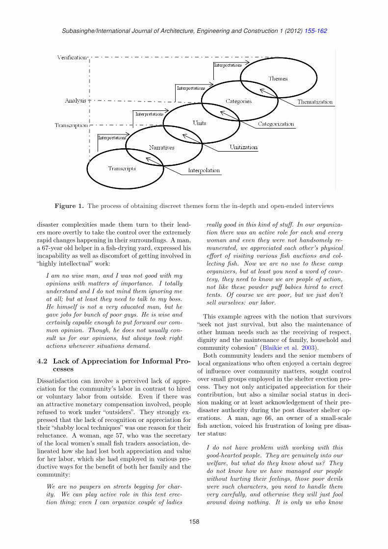
Subasinghe/International Journal of Architecture, Engineering and Construction 1 (2012) 155-162
Figure 1. The process of obtaining discreet themes form the in-depth and open-ended interviews
disaster complexities made them turn to their lead-ers more overtly to take the control over the extremelyrapid changes happening in their surroundings. A man,a 67-year old helper in a fish-drying yard, expressed hisincapability as well as discomfort of getting involved in“highly intellectual” work:
I am no wise man, and I was not good with myopinions with matters of importance. I totallyunderstand and I do not mind them ignoring meat all; but at least they need to talk to my boss.He himself is not a very educated man, but hegave jobs for bunch of poor guys. He is wise andcertainly capable enough to put forward our com-mon opinion. Though, he does not usually con-sult us for our opinions, but always took rightactions whenever situations demand.
4.2 Lack of Appreciation for Informal Pro-cesses
Dissatisfaction can involve a perceived lack of appre-ciation for the community’s labor in contrast to hiredor voluntary labor from outside. Even if there wasan attractive monetary compensation involved, peoplerefused to work under “outsiders”. They strongly ex-pressed that the lack of recognition or appreciation fortheir “shabby local techniques” was one reason for theirreluctance. A woman, age 57, who was the secretaryof the local women’s small fish traders association, de-lineated how she had lost both appreciation and valuefor her labor, which she had employed in various pro-ductive ways for the benefit of both her family and thecommunity:
We are no paupers on streets begging for char-ity. We can play active role in this tent erec-tion thing; even I can organize couple of ladies
really good in this kind of stuff. In our organiza-tion there was an active role for each and everywoman and even they were not handsomely re-munerated, we appreciated each other’s physicaleffort of visiting various fish auctions and col-lecting fish. Now we are no use to these camporganizers, but at least you need a word of cour-tesy, they need to know we are people of action,not like these powder puff babies hired to erecttents. Of course we are poor, but we just don’tsell ourselves: our labor.
This example agrees with the notion that survivors“seek not just survival, but also the maintenance ofother human needs such as the receiving of respect,dignity and the maintenance of family, household andcommunity cohesion” (Blaikie et al. 2003).Both community leaders and the senior members of
local organizations who often enjoyed a certain degreeof influence over community matters, sought controlover small groups employed in the shelter erection pro-cess. They not only anticipated appreciation for theircontribution, but also a similar social status in deci-sion making or at least acknowledgement of their pre-disaster authority during the post disaster shelter op-erations. A man, age 66, an owner of a small-scalefish auction, voiced his frustration of losing pre disas-ter status:
I do not have problem with working with thisgood-hearted people. They are genuinely into ourwelfare, but what do they know about us? Theydo not know how we have managed our peoplewithout hurting their feelings, those poor devilswere such characters, you need to handle themvery carefully, and otherwise they will just foolaround doing nothing. It is only us who know
158
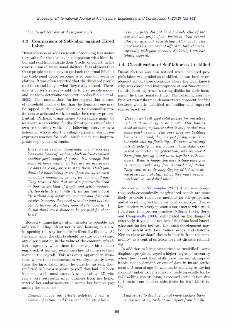
Subasinghe/International Journal of Architecture, Engineering and Construction 1 (2012) 155-162
how to get best out of these poor souls.
4.3 Comparison of Self-labor against HiredLabor
Dissatisfaction arises as a result of receiving less mone-tary value for their labor, in comparison with hired la-bor and skill from outside their “circle” or cohort, in theconstruction of transitional shelters. It is obvious thatthese people need money to get back to normal life, butthe traditional donor response is to pass out seeds orclothes. It was often reported that the displaced peoplesold those and bought what they really needed. There-fore, a better strategy would be to give people moneyand let them determine their own needs (Blaikie et al.2003). The same authors further suggest that sourcesof household income other than the dominant one maybe tapped, such as wage labor, petty commodity pro-duction or artisanal work, to make the recovery processfruitful. Perhaps, losing money to strangers might beas severe as receiving charity for staying out of theirown re-sheltering work. The following interview by afisherman who is also the village carpenter aka masonexpresses reaction for both unusable aids and inappro-priate deployment of funds:
It just drives us mad, doing nothing and receivingloads and loads of clothes, which at least can lastanother good couple of years. It’s strange thatsome of those winter clothes are no use besidewe don’t have any space to store them. Don’t youthink it’s humiliating to see these outsiders earnridiculous amount of money for doing nothing.They treat us like that we are practically deador that we are kind of fragile and brittle materi-als, too delicate to handle. If we can lead a goodlife without help before the tsunami and if we cansurvive tsunami, they need to understand that wecan do this bit of putting some shelter over us. Ido not think it’s a shame to be got paid for that.Is it?
Recovery immediately after disaster is possible notonly via building infrastructure and housing, but alsoin opening the way for more resilient livelihoods. Atthe same time, the efforts should be sure not to causeany discrimination in the value of the community’s ef-fort, especially when there is outside or hired laboremployed. A few expressed open hesitation to see theirname in the payroll. This was quite apparent in situa-tions where their remuneration was significantly lowerthan the hired labor from the outside; instead, theypreferred to have a separate payroll that had not beenimplemented in most cases. A woman of age 37, whoran a very successful small business from her home,uttered her embarrassment in seeing her humble payamong the outsiders:
Tsunami made me utterly helpless, I am awoman of action, and I ran such a lucrative busi-
ness, my peers did not have a single clue of thesize and the profit of the business. You cannotafford to give out such details, Can you? Theplace like this one cannot afford to take chances,especially with your income. Suddenly I am liketotally exposed.
4.4 Classification of Self-labor as Unskilled
Dissatisfaction was also noticed when displaced peo-ple’s labor was graded as unskilled. It was further ev-idence that on those occasions where the local knowl-edge was considered inappropriate or not “in-demand”,the displaced expressed a strong dislike for their hous-ing in the transitional settings. The following interviewby a veteran fisherman demonstrates apparent conflictbetween what is identified as familiar and importedshelter practices.
“Haven’t we built good solid houses for ourselveswithout those lousy techniques? Our housesstood so many cyclones; what it only needed wassome quick repair. The ones they are buildingfor us is no grand, they are just flashy, expensivebut rigid with no flexibility. We never hired anyoutside help to do our houses, these skills werepassed generation to generation, and we learntthem from just by doing them together with ourelders. What is happening here is they only giveus crappy work; any fool is capable of doing.They want us to do only digging of holes, clear-ing of site kind of stuff, which they mark in theirnotebooks as ’unskilled labor’. ”
As averred by Subasinghe (2011), there is a dangerthat socio-economically marginalized people are morelikely to doubt their own methods for self-protection,and stop relying on their own local knowledge. There-fore, modern recovery measures must merge with tradi-tional and time-proven practices (Chung 1987). Berkeand Campanella (2006) deliberated on the danger ofexternally driven plans not benefiting from local knowl-edge and further indicate that such development maybe inconsistent with local values, needs, and customs.Key to these authors’ theses is “buy-in from the com-munity” as a central criterion for post-disaster rebuild-ing.In addition to being categorized as “unskilled”, some
displaced people conveyed a higher degree of insecuritywhen they found their skills were less useful, unprof-itable, not in demand or out of date in future settle-ments. A man of age 66, who made his living by sawingcoconut timber using traditional tools especially for lo-cal dwelling construction, expressed intimidation dueto threats from efficient substitutes for his “skilled la-bor”:
I am scared to death, I do not know whether thereis any use of my tools at all. Apart from family,
159
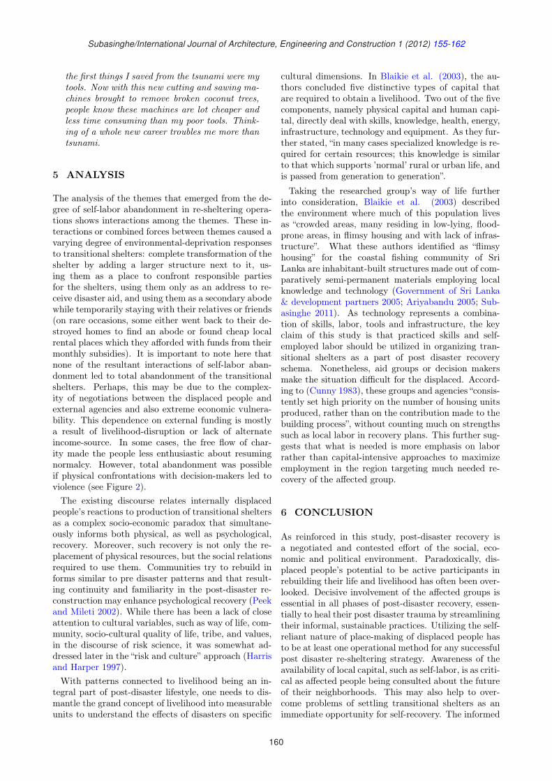
Subasinghe/International Journal of Architecture, Engineering and Construction 1 (2012) 155-162
the first things I saved from the tsunami were mytools. Now with this new cutting and sawing ma-chines brought to remove broken coconut trees,people know these machines are lot cheaper andless time consuming than my poor tools. Think-ing of a whole new career troubles me more thantsunami.
5 ANALYSIS
The analysis of the themes that emerged from the de-gree of self-labor abandonment in re-sheltering opera-tions shows interactions among the themes. These in-teractions or combined forces between themes caused avarying degree of environmental-deprivation responsesto transitional shelters: complete transformation of theshelter by adding a larger structure next to it, us-ing them as a place to confront responsible partiesfor the shelters, using them only as an address to re-ceive disaster aid, and using them as a secondary abodewhile temporarily staying with their relatives or friends(on rare occasions, some either went back to their de-stroyed homes to find an abode or found cheap localrental places which they afforded with funds from theirmonthly subsidies). It is important to note here thatnone of the resultant interactions of self-labor aban-donment led to total abandonment of the transitionalshelters. Perhaps, this may be due to the complex-ity of negotiations between the displaced people andexternal agencies and also extreme economic vulnera-bility. This dependence on external funding is mostlya result of livelihood-disruption or lack of alternateincome-source. In some cases, the free flow of char-ity made the people less enthusiastic about resumingnormalcy. However, total abandonment was possibleif physical confrontations with decision-makers led toviolence (see Figure 2).The existing discourse relates internally displaced
people’s reactions to production of transitional sheltersas a complex socio-economic paradox that simultane-ously informs both physical, as well as psychological,recovery. Moreover, such recovery is not only the re-placement of physical resources, but the social relationsrequired to use them. Communities try to rebuild informs similar to pre disaster patterns and that result-ing continuity and familiarity in the post-disaster re-construction may enhance psychological recovery (Peekand Mileti 2002). While there has been a lack of closeattention to cultural variables, such as way of life, com-munity, socio-cultural quality of life, tribe, and values,in the discourse of risk science, it was somewhat ad-dressed later in the “risk and culture” approach (Harrisand Harper 1997).With patterns connected to livelihood being an in-
tegral part of post-disaster lifestyle, one needs to dis-mantle the grand concept of livelihood into measurableunits to understand the effects of disasters on specific
cultural dimensions. In Blaikie et al. (2003), the au-thors concluded five distinctive types of capital thatare required to obtain a livelihood. Two out of the fivecomponents, namely physical capital and human capi-tal, directly deal with skills, knowledge, health, energy,infrastructure, technology and equipment. As they fur-ther stated, “in many cases specialized knowledge is re-quired for certain resources; this knowledge is similarto that which supports ’normal’ rural or urban life, andis passed from generation to generation”.
Taking the researched group’s way of life furtherinto consideration, Blaikie et al. (2003) describedthe environment where much of this population livesas “crowded areas, many residing in low-lying, flood-prone areas, in flimsy housing and with lack of infras-tructure”. What these authors identified as “flimsyhousing” for the coastal fishing community of SriLanka are inhabitant-built structures made out of com-paratively semi-permanent materials employing localknowledge and technology (Government of Sri Lanka& development partners 2005; Ariyabandu 2005; Sub-asinghe 2011). As technology represents a combina-tion of skills, labor, tools and infrastructure, the keyclaim of this study is that practiced skills and self-employed labor should be utilized in organizing tran-sitional shelters as a part of post disaster recoveryschema. Nonetheless, aid groups or decision makersmake the situation difficult for the displaced. Accord-ing to (Cunny 1983), these groups and agencies “consis-tently set high priority on the number of housing unitsproduced, rather than on the contribution made to thebuilding process”, without counting much on strengthssuch as local labor in recovery plans. This further sug-gests that what is needed is more emphasis on laborrather than capital-intensive approaches to maximizeemployment in the region targeting much needed re-covery of the affected group.
6 CONCLUSION
As reinforced in this study, post-disaster recovery isa negotiated and contested effort of the social, eco-nomic and political environment. Paradoxically, dis-placed people’s potential to be active participants inrebuilding their life and livelihood has often been over-looked. Decisive involvement of the affected groups isessential in all phases of post-disaster recovery, essen-tially to heal their post disaster trauma by streamliningtheir informal, sustainable practices. Utilizing the self-reliant nature of place-making of displaced people hasto be at least one operational method for any successfulpost disaster re-sheltering strategy. Awareness of theavailability of local capital, such as self-labor, is as criti-cal as affected people being consulted about the futureof their neighborhoods. This may also help to over-come problems of settling transitional shelters as animmediate opportunity for self-recovery. The informed
160
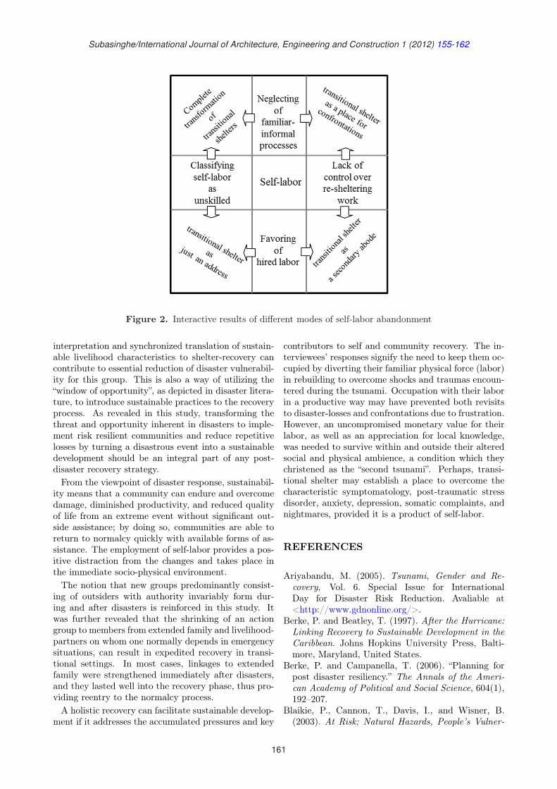
Subasinghe/International Journal of Architecture, Engineering and Construction 1 (2012) 155-162
Figure 2. Interactive results of different modes of self-labor abandonment
interpretation and synchronized translation of sustain-able livelihood characteristics to shelter-recovery cancontribute to essential reduction of disaster vulnerabil-ity for this group. This is also a way of utilizing the“window of opportunity”, as depicted in disaster litera-ture, to introduce sustainable practices to the recoveryprocess. As revealed in this study, transforming thethreat and opportunity inherent in disasters to imple-ment risk resilient communities and reduce repetitivelosses by turning a disastrous event into a sustainabledevelopment should be an integral part of any post-disaster recovery strategy.From the viewpoint of disaster response, sustainabil-
ity means that a community can endure and overcomedamage, diminished productivity, and reduced qualityof life from an extreme event without significant out-side assistance; by doing so, communities are able toreturn to normalcy quickly with available forms of as-sistance. The employment of self-labor provides a pos-itive distraction from the changes and takes place inthe immediate socio-physical environment.The notion that new groups predominantly consist-
ing of outsiders with authority invariably form dur-ing and after disasters is reinforced in this study. Itwas further revealed that the shrinking of an actiongroup to members from extended family and livelihood-partners on whom one normally depends in emergencysituations, can result in expedited recovery in transi-tional settings. In most cases, linkages to extendedfamily were strengthened immediately after disasters,and they lasted well into the recovery phase, thus pro-viding reentry to the normalcy process.A holistic recovery can facilitate sustainable develop-
ment if it addresses the accumulated pressures and key
contributors to self and community recovery. The in-terviewees’ responses signify the need to keep them oc-cupied by diverting their familiar physical force (labor)in rebuilding to overcome shocks and traumas encoun-tered during the tsunami. Occupation with their laborin a productive way may have prevented both revisitsto disaster-losses and confrontations due to frustration.However, an uncompromised monetary value for theirlabor, as well as an appreciation for local knowledge,was needed to survive within and outside their alteredsocial and physical ambience, a condition which theychristened as the “second tsunami”. Perhaps, transi-tional shelter may establish a place to overcome thecharacteristic symptomatology, post-traumatic stressdisorder, anxiety, depression, somatic complaints, andnightmares, provided it is a product of self-labor.
REFERENCES
Ariyabandu, M. (2005). Tsunami, Gender and Re-covery, Vol. 6. Special Issue for InternationalDay for Disaster Risk Reduction. Avaliable at<http://www.gdnonline.org/>.
Berke, P. and Beatley, T. (1997). After the Hurricane:Linking Recovery to Sustainable Development in theCaribbean. Johns Hopkins University Press, Balti-more, Maryland, United States.
Berke, P. and Campanella, T. (2006). “Planning forpost disaster resiliency.” The Annals of the Ameri-can Academy of Political and Social Science, 604(1),192–207.
Blaikie, P., Cannon, T., Davis, I., and Wisner, B.(2003). At Risk; Natural Hazards, People’s Vulner-
161

Subasinghe/International Journal of Architecture, Engineering and Construction 1 (2012) 155-162
ability and Disasters. Routledge, London, UnitedKingdom.
Bland, H., O’Leary, S., Farinaro, E., and Trevisan, M.(1996). “Long term psychological effects of naturaldisasters.” Psychosomatic Medicine, 58(1), 18–24.
Burroughs, J., Shippee, G., and Wakefield, S. (1980).“Dissonance theory revisited: Perception of environ-mental hazards in residential areas.” Environmentand Behaviour, 12(1), 33–51.
Chung, J. . (1987). “Fiji, land of tropical cyclones andhurricanes: A case study of agricultural rehabilita-tion.” Disasters, 11, 40–48.
Cunny, F. (1983). Disasters and Development. OxfordUniversity press, Oxford, United Kingdom.
Davis, I. (2006). Vernacular Architecture in the TwentyFirst Century, Theory, Education and Practice. Tay-lor & Francis, New York, United States, ChapterSheltering from Extreme Hazards, 145–154.
Fernando, U. and Hilhort, D. (2006). “Everyday prac-tices of humanitarian aid: Tsunami response in SriLanka.” Development in Practice, 16(3-4), 292–302.
Fischoff, B., Sevenson, O., and Slovic, P. (1988). Hand-book of Environmental Psychology, Vol. 2. Wiley,New York, United States, Chapter Active responsesto environmental hazards: Perceptions and decision-making, 1089–1133.
Flint, M. and Goyder, H. (2006). Funding the TsunamiResponse. Tsunami Evaluation Coalition, London,United Kingdom.
Government of Sri Lanka & development partners(2005). Post tsunami Recovery and Reconstruc-tion. Retrieved 09/01/2009 from. Avaliable at<http://siteresources.worldbank.org/INTTSUNAMI/Resources/srilankareport-dec05.pdf> (accessed09/01/2009).
Harris, S. G. and Harper, B. L. (1997). “A native amer-ican exposure scenario.” Risk Analysis, 17(6), 789–795.
Hewitt, K. (1997). Regions of Risk: A GeographicalIntroduction to Disasters. Longman, Harlow, Essex,United Kingdom.
Morrow, B. H. (1999). “Identifying and mapping com-munity vulnerability.” Disasters, 23(1), 1–18.
Peek, L. and Mileti, D. (2002). Handbook of Environ-mental psychology, Vol. 1. John Wiley & Sons Inc.,New York, United States, Chapter The History andfuture of disaster research, 511–524.
Porfiriev, N. (1995). “Disasters and disaster areas:Methodological issues of definition and delineation.”International Journal of mass disasters, 13(3), 285–304.
Sommer, R. (1969). Personal Space. Prentice-Hall, En-glewood Cliffs, New Jersey, United States.
Stirrat, R. L. (1977). “The social organization of fishingin a Sinhalese village, Ethnos.” Journal of Anthropol-ogy, 42(3-4), 122–148.
Subasinghe, C. (2011). Rebuilding for Sustainability:Spatial Analysis of Bolivar Peninsula after Hurri-cane Ike. Doctoral dissertation, Texas A&M Univer-sity, Texas, United States.
Task Force for Rebuilding the Nation (2005).Post Tsunami Recovery and Reconstruction Strat-egy: District Wise Post Tsunami Rehabilita-tion and Reconstruction Projects. Avaliable at<http://tafren.wow.lk/> (accessed 12/11/2009).
Wickramasinghe, A. (2005). “Tsunami: Building thenation through reciprocity while reconstructing theaffected areas in Sri Lanka.” Local Environment,10(5), 543–549.
162
International Journal of Architecture, Engineering and ConstructionVol 1, No 3, September 2012, 163-173
Automated Productivity Measurement Model of
Two-dimensional Earthmoving-equipment Operations
Ronie Navon∗, Simon Khoury, Yerach Doytsher
National Building Research Institute, Faculty of Civil and Environmental Engineering,
Israel Institute of Technology, Technion City, Haifa 32000, Israel
Abstract: Manual control of road construction is expensive, time consuming and error prone. Hence it is doneinfrequently, or is based on rough estimates - the previous stage of this research attempted to automate thisprocess. The research developed a model which had to assume that work progresses according to plans. Thisassumption permitted the use of predetermined work envelops. The present model introduces a new approach- a dynamic work envelop - which also uses the same type of data as the previous model, i.e., the location ofthe equipment as a function of time measured by GPS. The model, which was developed in a GeographicalInformation System environment, determines both the area of the work and the time it took to perform it. Apilot field test showed that this model can generate control information with a deviation of +15% - this deviationcan be meaningfully increased if averaged over a number of days. An economic analysis of the proposed systemshows that it is more economical than the manual methods, especially if the control information is needed at ahigher frequency than biweekly.
Keywords: Automation, control methods, data collection, earthmoving, GPS, monitoring, road construction
DOI: 10.7492/IJAEC.2012.018
1 INTRODUCTION
Earthmoving operations rely on the skills of the opera-tors and surveyors and involve a lot of staking and re-staking, which causes a significant delay. Often opera-tors proceed with the operation without any resettingof stakes because surveyors are not always available onsites. This causes serious deviations from the desireddesign surface, rework (Han et al. 2005) as well as devi-ation from the planned productivity and the inevitabledelays and cost escalations. This procedure is, there-fore, expensive, time-consuming and unproductive.Recently, earthmoving operations are experiencing
impressive advancements, which improve the accuracyand quality of their output, increase the efficiency ofoperations, and save costs. These advancements in-clude measuring various parameters relating to thehealth and maintenance of the earthmoving equipment- such as valves pressure, and weight of bucket (Kannanand Vorster 2000; Maio et al. 2000) - as well as contin-uously monitoring the location of the equipment dur-ing its operation (Caterpillar 2007; JohnDeere 2007;Peyret and Tasky 2004; Taylor and Tometich 2003;
Trimble 2007).The above impressive achievements deal mainly with
issues such as the automation of quality assurance (e.g.,asphalt compaction), or the reduction of the survey-ing costs during earthmoving operations. Very littleattention has been given to automate the measure-ment of managerial parameters such as progress andproductivity. This paper describes a model that usesGPS technology for automated data collection to pro-duce information needed for efficient monitoring of two-dimensional earthmoving-equipment operations. Themodel uses algorithms based on the dynamic work en-velop approach to convert the collected data into con-trol information and presents it in terms of duration(or progress), productivity, and quantities.
2 EARLIER STAGES IN AUTOMATEDROAD CONSTRUCTION CONTROL
The previous stage of this research developed a modelwhich assumed that at the planning stage the road isdivided into work sections (WS) - areas where work on
*Corresponding author. Email: [email protected]
163
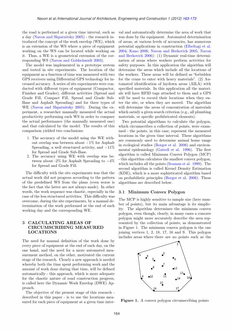
Navon et al./International Journal of Architecture, Engineering and Construction 1 (2012) 163-173
the road is performed at a given time interval, such asa day (Navon and Shpatnitsky 2005) - the research in-troduced the concept of the work envelop (WE), whichis an extension of the WS where a piece of equipmentworking on the WS can be located while working onit. Thus, a WE is a geometrical extension of the cor-responding WS (Navon and Goldschmidt 2003).The model was implemented in a prototype system
and tested in site experiments. The location of theequipment as a function of time was measured with twoGPS receivers using Differential GPS technology for in-creased accuracy. A series of site experiments were con-ducted with different types of equipment (Compactor,Finisher and Grader), different activities (Spread andGrade Fill, Compact Fill, Spread and Grade Sub-Base and Asphalt Spreading) and for three types ofWE (Navon and Shpatnitsky 2005). During the ex-periment, a researcher manually measured the actualproductivity performing each WS in order to comparethe actual performance (the manually measured one)and that calculated by the model. The results of thiscomparison yielded two conclusions:
1. The accuracy of the model using the WE with-out overlap was between about +1% for AsphaltSpreading, a well structured activity, and +11%for Spread and Grade Sub-Base.
2. The accuracy using WE with overlap was be-tween about -2% for Asphalt Spreading to +4%for Spread and Grade Fill.
The difficulty with the site experiments was that theactual work did not progress according to the patternof the predefined WS from the plans (even worse isthe fact that the latter are not always made). In otherwords, the work sequence was chaotic, especially in thecase of the less structured activities. This difficulty wasovercome, during the site experiments, by a manual de-termination of the work performed at the end of eachworking day and the corresponding WE.
3 CALCULATING AREAS OFCIRCUMSCRIBING MEASUREDLOCATIONS
The need for manual definition of the work done byevery piece of equipment at the end of each day, on theone hand, and the need for a more automated mea-surement method, on the other, motivated the currentstage of the research. Clearly a new approach is neededwhereby both the time spent performing work and theamount of work done during that time, will be definedautomatically - this approach, which is more adequatefor the chaotic nature of road construction progress,is called here the Dynamic Work Envelop (DWE) Ap-proach.The objective of the present stage of this research -
described in this paper - is to use the locations mea-sured for each piece of equipment at a given time inter-
val and automatically determine the area of work thatwas done by the equipment. Automated determinationof areas, at various levels of accuracies, has numerouspotential applications in construction (Elbeltagi et al.2004; Kano 2006; Navon and Berkovich 2005; Navonand Berkovich 2006): (1) Dynamic real-time determi-nation of areas where workers perform activities forsafety purposes. In this application the algorithm willdetermine the areas which include all the locations ofthe workers. These areas will be defined as “forbiddenfor the crane to enter with heavy materials”. (2) Au-tomated identification of laydown areas (AILA) withspecified materials. In this application all the materi-als will have RFID tags attached to them and a GPSwill be used to record their locations when they en-ter the site, or when they are moved. The algorithmwill determine the areas of concentration of materialswhich satisfy a given search criterion (e.g., all plumbingmaterials, or specific prefabricated elements).Two potential algorithms to calculate the polygon,
which circumscribes a collection of points, were exam-ined - the points, in this case, represent the measuredlocations in the given time interval. These algorithmsare commonly used to determine animal home rangein ecological studies (Borger et al. 2006) and environ-mental epidemiology (Gatrell et al. 1996). The firstalgorithm is called Minimum Convex Polygon (MCP)- this algorithm calculates the smallest convex polygon,which includes all the points (Seaman et al. 1999). Thesecond algorithm is called Kernel Density Estimation(KDE), which is a more sophisticated algorithm basedon probabilistic principles (Borger et al. 2006). Thesealgorithms are described below.
3.1 Minimum Convex Polygon
The MCP is highly sensitive to sample size (here num-ber of points), but its main advantage is its simplic-ity. The algorithm determines the minimum convexpolygon, even though, clearly, in many cases a concavepolygon might more accurately describe the area rep-resented by the collection of points, as demonstratedin Figure 1. The minimum convex polygon is the onejoining vertices 1, 2, 18, 17, 16 and 9. This polygonincludes areas where there are no points such as the
Figure 1. A convex polygon circumscribing points
164
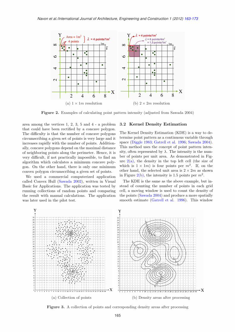
Navon et al./International Journal of Architecture, Engineering and Construction 1 (2012) 163-173
(a) 1× 1m resolution (b) 2× 2m resolution
Figure 2. Examples of calculating point pattern intensity (adjusted from Sawada 2004)
area among the vertices 1, 2, 3, 5 and 4 - a problemthat could have been rectified by a concave polygon.The difficulty is that the number of concave polygonscircumscribing a given set of points is very large and itincreases rapidly with the number of points. Addition-ally, concave polygons depend on the maximal distanceof neighboring points along the perimeter. Hence, it isvery difficult, if not practically impossible, to find analgorithm which calculates a minimum concave poly-gon. On the other hand, there is only one minimumconvex polygon circumscribing a given set of points.We used a commercial computerized application
called Convex Hull (Sawada 2002), written in VisualBasic for Applications. The application was tested byrunning collections of random points and comparingthe result with manual calculations. The applicationwas later used in the pilot test.
3.2 Kernel Density Estimation
The Kernel Density Estimation (KDE) is a way to de-termine point pattern as a continuous variable throughspace (Diggle 1983; Gatrell et al. 1996; Sawada 2004).This method uses the concept of point pattern inten-sity, often represented by λ. The intensity is the num-ber of points per unit area. As demonstrated in Fig-ure 2(a), the density in the top left cell (the size ofwhich is 1 × 1m) is four points per m2. If, on theother hand, the selected unit area is 2 × 2m as shownin Figure 2(b), the intensity is 1.5 points per m2.The KDE is the same as the above example, but in-
stead of counting the number of points in each gridcell, a moving window is used to count the density ofthe points (Sawada 2004) and produce a more spatiallysmooth estimate (Gatrell et al. 1996). This window
(a) Collection of points (b) Density areas after processing
Figure 3. A collection of points and corresponding density areas after processing
165
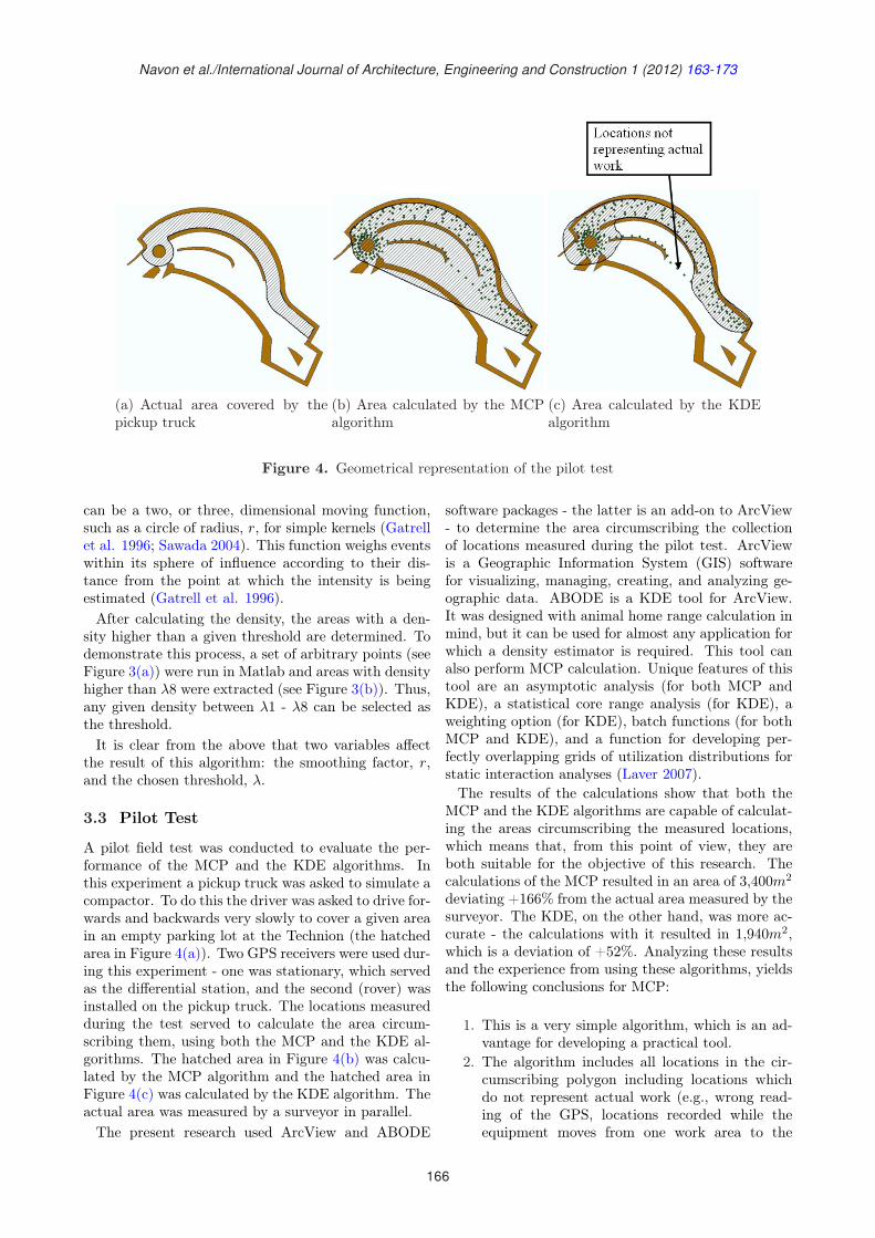
Navon et al./International Journal of Architecture, Engineering and Construction 1 (2012) 163-173
(a) Actual area covered by thepickup truck
(b) Area calculated by the MCPalgorithm
(c) Area calculated by the KDEalgorithm
Figure 4. Geometrical representation of the pilot test
can be a two, or three, dimensional moving function,such as a circle of radius, r, for simple kernels (Gatrellet al. 1996; Sawada 2004). This function weighs eventswithin its sphere of influence according to their dis-tance from the point at which the intensity is beingestimated (Gatrell et al. 1996).After calculating the density, the areas with a den-
sity higher than a given threshold are determined. Todemonstrate this process, a set of arbitrary points (seeFigure 3(a)) were run in Matlab and areas with densityhigher than λ8 were extracted (see Figure 3(b)). Thus,any given density between λ1 - λ8 can be selected asthe threshold.It is clear from the above that two variables affect
the result of this algorithm: the smoothing factor, r,and the chosen threshold, λ.
3.3 Pilot Test
A pilot field test was conducted to evaluate the per-formance of the MCP and the KDE algorithms. Inthis experiment a pickup truck was asked to simulate acompactor. To do this the driver was asked to drive for-wards and backwards very slowly to cover a given areain an empty parking lot at the Technion (the hatchedarea in Figure 4(a)). Two GPS receivers were used dur-ing this experiment - one was stationary, which servedas the differential station, and the second (rover) wasinstalled on the pickup truck. The locations measuredduring the test served to calculate the area circum-scribing them, using both the MCP and the KDE al-gorithms. The hatched area in Figure 4(b) was calcu-lated by the MCP algorithm and the hatched area inFigure 4(c) was calculated by the KDE algorithm. Theactual area was measured by a surveyor in parallel.The present research used ArcView and ABODE
software packages - the latter is an add-on to ArcView- to determine the area circumscribing the collectionof locations measured during the pilot test. ArcViewis a Geographic Information System (GIS) softwarefor visualizing, managing, creating, and analyzing ge-ographic data. ABODE is a KDE tool for ArcView.It was designed with animal home range calculation inmind, but it can be used for almost any application forwhich a density estimator is required. This tool canalso perform MCP calculation. Unique features of thistool are an asymptotic analysis (for both MCP andKDE), a statistical core range analysis (for KDE), aweighting option (for KDE), batch functions (for bothMCP and KDE), and a function for developing per-fectly overlapping grids of utilization distributions forstatic interaction analyses (Laver 2007).The results of the calculations show that both the
MCP and the KDE algorithms are capable of calculat-ing the areas circumscribing the measured locations,which means that, from this point of view, they areboth suitable for the objective of this research. Thecalculations of the MCP resulted in an area of 3,400m2
deviating +166% from the actual area measured by thesurveyor. The KDE, on the other hand, was more ac-curate - the calculations with it resulted in 1,940m2,which is a deviation of +52%. Analyzing these resultsand the experience from using these algorithms, yieldsthe following conclusions for MCP:
1. This is a very simple algorithm, which is an ad-vantage for developing a practical tool.
2. The algorithm includes all locations in the cir-cumscribing polygon including locations whichdo not represent actual work (e.g., wrong read-ing of the GPS, locations recorded while theequipment moves from one work area to the
166
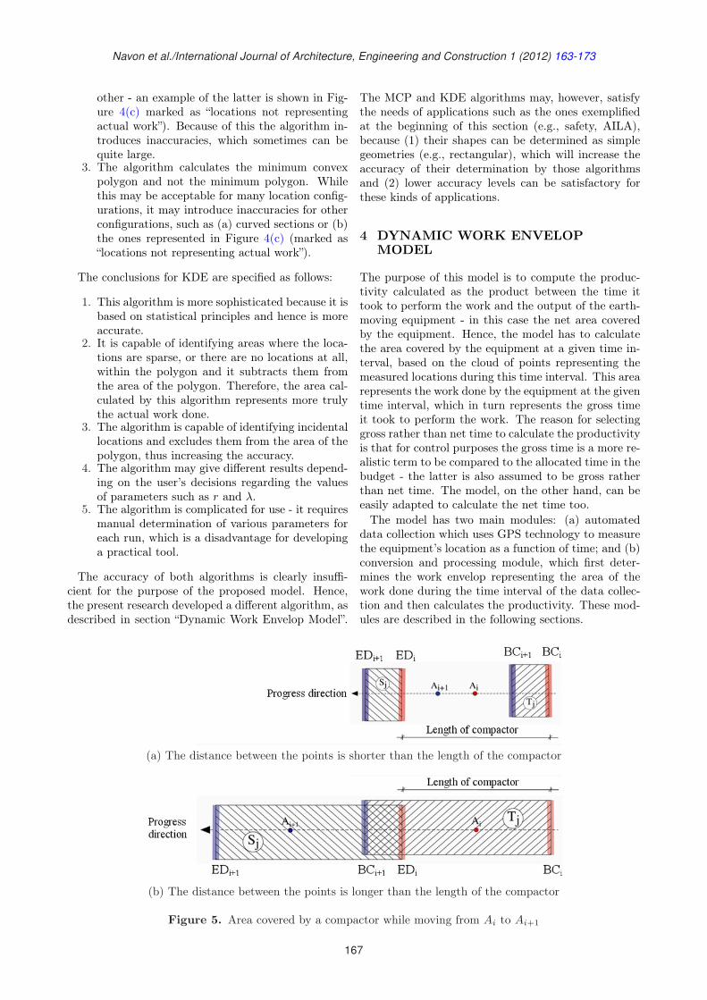
Navon et al./International Journal of Architecture, Engineering and Construction 1 (2012) 163-173
other - an example of the latter is shown in Fig-ure 4(c) marked as “locations not representingactual work”). Because of this the algorithm in-troduces inaccuracies, which sometimes can bequite large.
3. The algorithm calculates the minimum convexpolygon and not the minimum polygon. Whilethis may be acceptable for many location config-urations, it may introduce inaccuracies for otherconfigurations, such as (a) curved sections or (b)the ones represented in Figure 4(c) (marked as“locations not representing actual work”).
The conclusions for KDE are specified as follows:
1. This algorithm is more sophisticated because it isbased on statistical principles and hence is moreaccurate.
2. It is capable of identifying areas where the loca-tions are sparse, or there are no locations at all,within the polygon and it subtracts them fromthe area of the polygon. Therefore, the area cal-culated by this algorithm represents more trulythe actual work done.
3. The algorithm is capable of identifying incidentallocations and excludes them from the area of thepolygon, thus increasing the accuracy.
4. The algorithm may give different results depend-ing on the user’s decisions regarding the valuesof parameters such as r and λ.
5. The algorithm is complicated for use - it requiresmanual determination of various parameters foreach run, which is a disadvantage for developinga practical tool.
The accuracy of both algorithms is clearly insuffi-cient for the purpose of the proposed model. Hence,the present research developed a different algorithm, asdescribed in section “Dynamic Work Envelop Model”.
The MCP and KDE algorithms may, however, satisfythe needs of applications such as the ones exemplifiedat the beginning of this section (e.g., safety, AILA),because (1) their shapes can be determined as simplegeometries (e.g., rectangular), which will increase theaccuracy of their determination by those algorithmsand (2) lower accuracy levels can be satisfactory forthese kinds of applications.
4 DYNAMIC WORK ENVELOPMODEL
The purpose of this model is to compute the produc-tivity calculated as the product between the time ittook to perform the work and the output of the earth-moving equipment - in this case the net area coveredby the equipment. Hence, the model has to calculatethe area covered by the equipment at a given time in-terval, based on the cloud of points representing themeasured locations during this time interval. This arearepresents the work done by the equipment at the giventime interval, which in turn represents the gross timeit took to perform the work. The reason for selectinggross rather than net time to calculate the productivityis that for control purposes the gross time is a more re-alistic term to be compared to the allocated time in thebudget - the latter is also assumed to be gross ratherthan net time. The model, on the other hand, can beeasily adapted to calculate the net time too.The model has two main modules: (a) automated
data collection which uses GPS technology to measurethe equipment’s location as a function of time; and (b)conversion and processing module, which first deter-mines the work envelop representing the area of thework done during the time interval of the data collec-tion and then calculates the productivity. These mod-ules are described in the following sections.
(a) The distance between the points is shorter than the length of the compactor
(b) The distance between the points is longer than the length of the compactor
Figure 5. Area covered by a compactor while moving from Ai to Ai+1
167
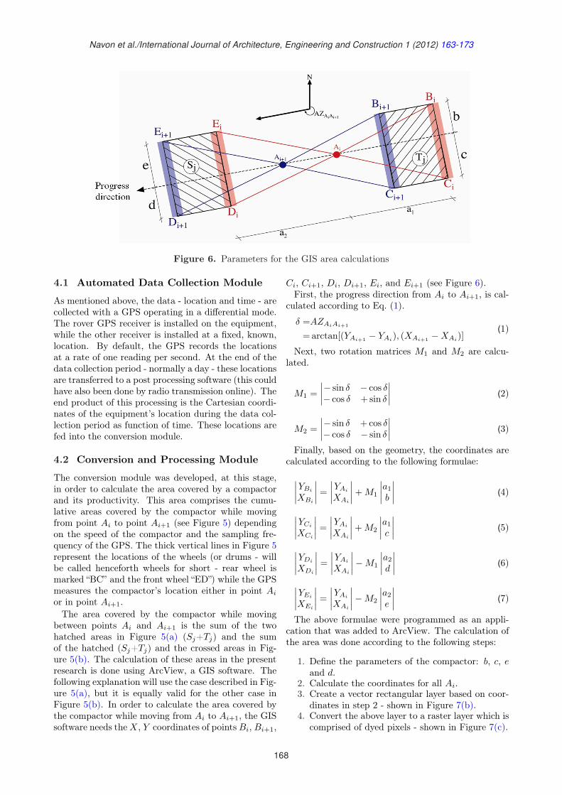
Navon et al./International Journal of Architecture, Engineering and Construction 1 (2012) 163-173
Figure 6. Parameters for the GIS area calculations
4.1 Automated Data Collection Module
As mentioned above, the data - location and time - arecollected with a GPS operating in a differential mode.The rover GPS receiver is installed on the equipment,while the other receiver is installed at a fixed, known,location. By default, the GPS records the locationsat a rate of one reading per second. At the end of thedata collection period - normally a day - these locationsare transferred to a post processing software (this couldhave also been done by radio transmission online). Theend product of this processing is the Cartesian coordi-nates of the equipment’s location during the data col-lection period as function of time. These locations arefed into the conversion module.
4.2 Conversion and Processing Module
The conversion module was developed, at this stage,in order to calculate the area covered by a compactorand its productivity. This area comprises the cumu-lative areas covered by the compactor while movingfrom point Ai to point Ai+1 (see Figure 5) dependingon the speed of the compactor and the sampling fre-quency of the GPS. The thick vertical lines in Figure 5represent the locations of the wheels (or drums - willbe called henceforth wheels for short - rear wheel ismarked “BC” and the front wheel “ED”) while the GPSmeasures the compactor’s location either in point Ai
or in point Ai+1.The area covered by the compactor while moving
between points Ai and Ai+1 is the sum of the twohatched areas in Figure 5(a) (Sj+Tj) and the sumof the hatched (Sj+Tj) and the crossed areas in Fig-ure 5(b). The calculation of these areas in the presentresearch is done using ArcView, a GIS software. Thefollowing explanation will use the case described in Fig-ure 5(a), but it is equally valid for the other case inFigure 5(b). In order to calculate the area covered bythe compactor while moving from Ai to Ai+1, the GISsoftware needs the X, Y coordinates of points Bi, Bi+1,
Ci, Ci+1, Di, Di+1, Ei, and Ei+1 (see Figure 6).First, the progress direction from Ai to Ai+1, is cal-
culated according to Eq. (1).
δ =AZAiAi+1
=arctan[(YAi+1 − YAi), (XAi+1 −XAi
)](1)
Next, two rotation matrices M1 and M2 are calcu-lated.
M1 =∣∣∣∣− sin δ − cos δ− cos δ +sin δ
∣∣∣∣ (2)
M2 =∣∣∣∣− sin δ +cos δ− cos δ − sin δ
∣∣∣∣ (3)
Finally, based on the geometry, the coordinates arecalculated according to the following formulae:
∣∣∣∣YBi
XBi
∣∣∣∣ =∣∣∣∣YAi
XAi
∣∣∣∣ + M1
∣∣∣∣a1
b
∣∣∣∣ (4)
∣∣∣∣YCi
XCi
∣∣∣∣ =∣∣∣∣YAi
XAi
∣∣∣∣ + M2
∣∣∣∣a1
c
∣∣∣∣ (5)
∣∣∣∣YDi
XDi
∣∣∣∣ =∣∣∣∣YAi
XAi
∣∣∣∣−M1
∣∣∣∣a2
d
∣∣∣∣ (6)
∣∣∣∣YEi
XEi
∣∣∣∣ =∣∣∣∣YAi
XAi
∣∣∣∣−M2
∣∣∣∣a2
e
∣∣∣∣ (7)
The above formulae were programmed as an appli-cation that was added to ArcView. The calculation ofthe area was done according to the following steps:
1. Define the parameters of the compactor: b, c, eand d.
2. Calculate the coordinates for all Ai.3. Create a vector rectangular layer based on coor-
dinates in step 2 - shown in Figure 7(b).4. Convert the above layer to a raster layer which is
comprised of dyed pixels - shown in Figure 7(c).
168
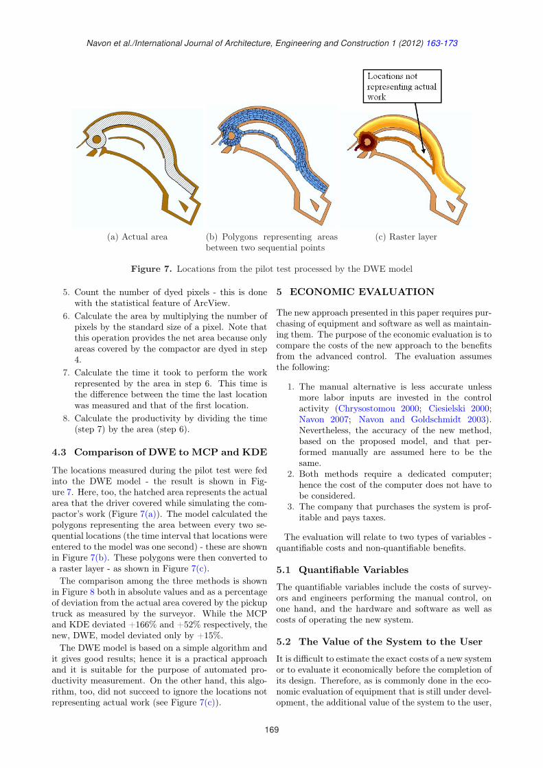
Navon et al./International Journal of Architecture, Engineering and Construction 1 (2012) 163-173
(a) Actual area (b) Polygons representing areasbetween two sequential points
(c) Raster layer
Figure 7. Locations from the pilot test processed by the DWE model
5. Count the number of dyed pixels - this is donewith the statistical feature of ArcView.
6. Calculate the area by multiplying the number ofpixels by the standard size of a pixel. Note thatthis operation provides the net area because onlyareas covered by the compactor are dyed in step4.
7. Calculate the time it took to perform the workrepresented by the area in step 6. This time isthe difference between the time the last locationwas measured and that of the first location.
8. Calculate the productivity by dividing the time(step 7) by the area (step 6).
4.3 Comparison of DWE to MCP and KDE
The locations measured during the pilot test were fedinto the DWE model - the result is shown in Fig-ure 7. Here, too, the hatched area represents the actualarea that the driver covered while simulating the com-pactor’s work (Figure 7(a)). The model calculated thepolygons representing the area between every two se-quential locations (the time interval that locations wereentered to the model was one second) - these are shownin Figure 7(b). These polygons were then converted toa raster layer - as shown in Figure 7(c).The comparison among the three methods is shown
in Figure 8 both in absolute values and as a percentageof deviation from the actual area covered by the pickuptruck as measured by the surveyor. While the MCPand KDE deviated +166% and +52% respectively, thenew, DWE, model deviated only by +15%.The DWE model is based on a simple algorithm and
it gives good results; hence it is a practical approachand it is suitable for the purpose of automated pro-ductivity measurement. On the other hand, this algo-rithm, too, did not succeed to ignore the locations notrepresenting actual work (see Figure 7(c)).
5 ECONOMIC EVALUATION
The new approach presented in this paper requires pur-chasing of equipment and software as well as maintain-ing them. The purpose of the economic evaluation is tocompare the costs of the new approach to the benefitsfrom the advanced control. The evaluation assumesthe following:
1. The manual alternative is less accurate unlessmore labor inputs are invested in the controlactivity (Chrysostomou 2000; Ciesielski 2000;Navon 2007; Navon and Goldschmidt 2003).Nevertheless, the accuracy of the new method,based on the proposed model, and that per-formed manually are assumed here to be thesame.
2. Both methods require a dedicated computer;hence the cost of the computer does not have tobe considered.
3. The company that purchases the system is prof-itable and pays taxes.
The evaluation will relate to two types of variables -quantifiable costs and non-quantifiable benefits.
5.1 Quantifiable Variables
The quantifiable variables include the costs of survey-ors and engineers performing the manual control, onone hand, and the hardware and software as well ascosts of operating the new system.
5.2 The Value of the System to the User
It is difficult to estimate the exact costs of a new systemor to evaluate it economically before the completion ofits design. Therefore, as is commonly done in the eco-nomic evaluation of equipment that is still under devel-opment, the additional value of the system to the user,
169
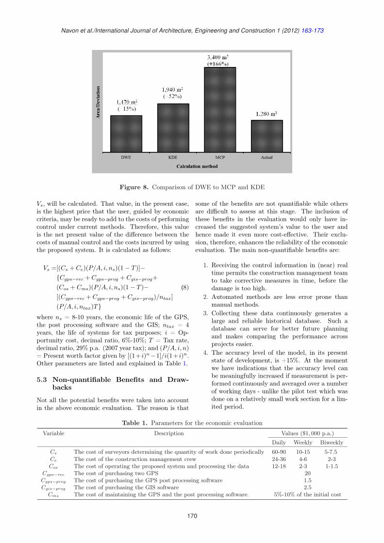
Navon et al./International Journal of Architecture, Engineering and Construction 1 (2012) 163-173
Figure 8. Comparison of DWE to MCP and KDE
Vs, will be calculated. That value, in the present case,is the highest price that the user, guided by economiccriteria, may be ready to add to the costs of performingcontrol under current methods. Therefore, this valueis the net present value of the difference between thecosts of manual control and the costs incurred by usingthe proposed system. It is calculated as follows:
Vs =[(Cs + Ce)(P/A, i, ns)(1− T )]−Cgps−rec + Cgps−prog + Cgis−prog+(Cos + Cms)(P/A, i, ns)(1− T )−[(Cgps−rec + Cgps−prog + Cgis−prog)/ntax](P/A, i, ntax)T
(8)
where ns = 8-10 years, the economic life of the GPS,the post processing software and the GIS; ntax = 4years, the life of systems for tax purposes; i = Op-portunity cost, decimal ratio, 6%-10%; T = Tax rate,decimal ratio, 29% p.a. (2007 year tax); and (P/A, i, n)= Present worth factor given by [(1+ i)n−1]/i(1+ i)n.Other parameters are listed and explained in Table 1.
5.3 Non-quantifiable Benefits and Draw-backs
Not all the potential benefits were taken into accountin the above economic evaluation. The reason is that
some of the benefits are not quantifiable while othersare difficult to assess at this stage. The inclusion ofthese benefits in the evaluation would only have in-creased the suggested system’s value to the user andhence made it even more cost-effective. Their exclu-sion, therefore, enhances the reliability of the economicevaluation. The main non-quantifiable benefits are:
1. Receiving the control information in (near) realtime permits the construction management teamto take corrective measures in time, before thedamage is too high.
2. Automated methods are less error prone thanmanual methods.
3. Collecting these data continuously generates alarge and reliable historical database. Such adatabase can serve for better future planningand makes comparing the performance acrossprojects easier.
4. The accuracy level of the model, in its presentstate of development, is +15%. At the momentwe have indications that the accuracy level canbe meaningfully increased if measurement is per-formed continuously and averaged over a numberof working days - unlike the pilot test which wasdone on a relatively small work section for a lim-ited period.
Table 1. Parameters for the economic evaluation
Variable Description Values ($1, 000 p.a.)
Daily Weekly Biweekly
Cs The cost of surveyors determining the quantity of work done periodically 60-90 10-15 5-7.5Ce The cost of the construction management crew 24-36 4-6 2-3Cos The cost of operating the proposed system and processing the data 12-18 2-3 1-1.5
Cgps−rec The cost of purchasing two GPS 20Cgps−prog The cost of purchasing the GPS post processing software 1.5Cgis−prog The cost of purchasing the GIS software 2.5
Cms The cost of maintaining the GPS and the post processing software. 5%-10% of the initial cost
170
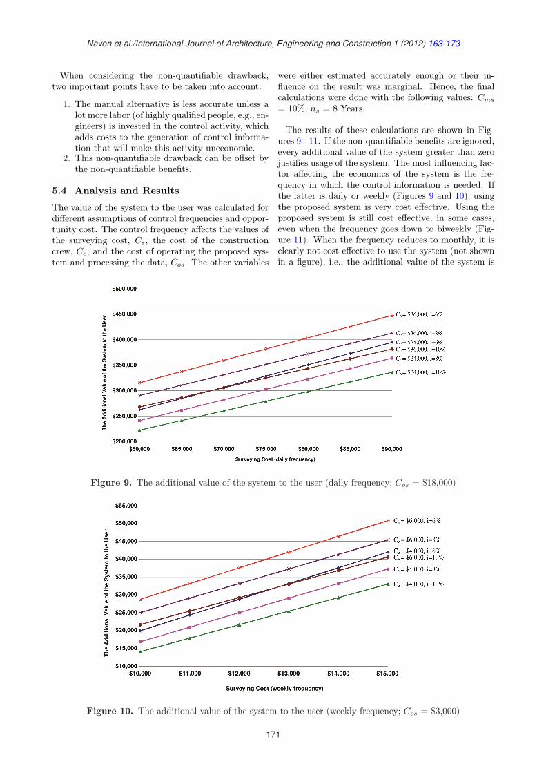
Navon et al./International Journal of Architecture, Engineering and Construction 1 (2012) 163-173
When considering the non-quantifiable drawback,two important points have to be taken into account:
1. The manual alternative is less accurate unless alot more labor (of highly qualified people, e.g., en-gineers) is invested in the control activity, whichadds costs to the generation of control informa-tion that will make this activity uneconomic.
2. This non-quantifiable drawback can be offset bythe non-quantifiable benefits.
5.4 Analysis and Results
The value of the system to the user was calculated fordifferent assumptions of control frequencies and oppor-tunity cost. The control frequency affects the values ofthe surveying cost, Cs, the cost of the constructioncrew, Ce, and the cost of operating the proposed sys-tem and processing the data, Cos. The other variables
were either estimated accurately enough or their in-fluence on the result was marginal. Hence, the finalcalculations were done with the following values: Cms
= 10%, ns = 8 Years.
The results of these calculations are shown in Fig-ures 9 - 11. If the non-quantifiable benefits are ignored,every additional value of the system greater than zerojustifies usage of the system. The most influencing fac-tor affecting the economics of the system is the fre-quency in which the control information is needed. Ifthe latter is daily or weekly (Figures 9 and 10), usingthe proposed system is very cost effective. Using theproposed system is still cost effective, in some cases,even when the frequency goes down to biweekly (Fig-ure 11). When the frequency reduces to monthly, it isclearly not cost effective to use the system (not shownin a figure), i.e., the additional value of the system is
Figure 9. The additional value of the system to the user (daily frequency; Cos = $18,000)
Figure 10. The additional value of the system to the user (weekly frequency; Cos = $3,000)
171
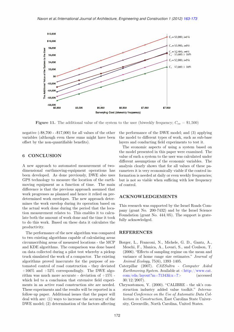
Navon et al./International Journal of Architecture, Engineering and Construction 1 (2012) 163-173
Figure 11. The additional value of the system to the user (biweekly frequency; Cos = $1,500)
negative (-$8,700 - -$17,000) for all values of the othervariables (although even these sums might have beenoffset by the non-quantifiable benefits).
6 CONCLUSION
A new approach to automated measurement of two-dimensional earthmoving-equipment operations hasbeen developed. As done previously, DWE also usesGPS technology to measure the location of the earth-moving equipment as a function of time. The maindifference is that the previous approach assumed thatwork progresses as planned and hence it relied on pre-determined work envelopes. The new approach deter-mines the work envelop during its operation based onthe actual work done during the period that the loca-tion measurement relates to. This enables it to calcu-late both the amount of work done and the time it tookto do this work. Based on these data it calculates theproductivity.The performance of the new algorithm was compared
to two existing algorithms capable of calculating areascircumscribing areas of measured locations - the MCPand KDE algorithms. The comparison was done basedon data collected during a pilot test whereby a pickuptruck simulated the work of a compactor. The existingalgorithms proved inaccurate for the purpose of au-tomated control of road construction - they deviated+166% and +52% correspondingly. The DWE algo-rithm was much more accurate - deviation of +15% -which led to a conclusion that extensive field experi-ments in an active road construction site are needed.These experiments and the results will be reported in afollow-up paper. Additional issues that the paper willdeal with are: (1) ways to increase the accuracy of theDWE model; (2) determination of the factors affecting
the performance of the DWE model; and (3) applyingthe model to different types of work, such as sub-baselayers and conducting field experiments to test it.The economic aspects of using a system based on
the model presented in this paper were examined. Thevalue of such a system to the user was calculated underdifferent assumptions of the economic variables. Theanalysis clearly shows that for all values of these pa-rameters it is very economically viable if the control in-formation is needed at daily or even weekly frequencies;but is not so viable when sufficing with low frequencyof control.
ACKNOWLEDGEMENTS
This research was supported by the Israel Roads Com-pany (grant No. 200-7432) and by the Israel ScienceFoundation (grant No. 444/05). The support is grate-fully acknowledged.
REFERENCES
Borger, L., Franconi, N., Michele, G. D., Gantz, A.,Meschi, F., Manica, A., Lovari, S., and Coulson, T.(2006). “Effects of sampling regime on the mean andvariance of home range size estimates.” Journal ofAnimal Ecology, 75(6), 1393–1405.
Caterpillar (2007). CAESultra - Computer AidedEarthmoving System. Available at <http://www.cat.com/cda/layout?m=71343&x=7> (accessed30/12/2007).
Chrysostomou, V. (2000). “CALIBRE - the uk’s con-struction industry added value toolkit.” Interna-tional Conference on the Use of Automatic Data Col-lection in Construction, East Carolina State Univer-sity, Greenville, North Carolina, United States.
172

Navon et al./International Journal of Architecture, Engineering and Construction 1 (2012) 163-173
Ciesielski, C. A. (2000). ADCIC - Automatic Data Col-lection in Construction. Haifa, Israel.
Diggle, P. J. (1983). Statistical Analysis of SpatialPoint Patterns. Academic Press, London, UnitedKingdom.
Elbeltagi, E., Hegazy, T., and Eldosouky, A. (2004).“Dynamic layout of construction temporary facili-ties considering safety.” Jounal of Construction En-gineering and Management, 130(4), 534–541.
Gatrell, A. C., Bailey, T. C., Diggle, P. J., and Rowling-son, B. S. (1996). “Spatial point pattern analysis andits application in geographical epidemiology.” Trans-actions of the Institute of British Geographers, 21(1),256–274.
Han, S. W., Lee, S. Y., and Halpin, D. W. (2005). “Pro-ductivity evaluation of conventional and gps-basedearthmoving systems using construction simulation.”Construction Research Congress, San Diego, UnitedStates, 178–182.
JohnDeere (2007). JDLink Machine Monitoring Sys-tem. Available at <http://www.deere.com/> (ac-cessed 29/10/2007).
Kannan, G. and Vorster, M. (2000). “Development ofan experience database for truck loading operations.”Journal of Construction Engineering and Manage-ment, 126(3), 201–209.
Kano, N. (2006). “Construction management tools us-ing 3D-CAD, virtual reality, RFID, and photogra-phy technologies.” Twenty Third International Sym-posium on Automation and Robotics in Construc-tion, Tokyo, Japan, 430–435.
Laver, P. (2007). ABODE: Density Estimation, HomeRange and Ecological Tools for ArcGIS. Available at<http://www.filebox.vt.edu/users/plaver/abode/home.html> (accessed 05/12/2007).
Maio, C., Schexnayder, C., Knutson, K., and Weber,S. (2000). “Probability distribution functions for con-struction simulation.” Journal of Construction Engi-neering and Management, 126(4), 285–292.
Navon, R. (2007). “Research in automated measure-ment of project performance indicators.” Automationin Construction, 16(2), 176–188.
Navon, R. and Berkovich, O. (2005). “Development andon site evaluation of an automated materials man-agement and control model.” Journal of Construc-tion Engineering and Management, 131(2), 1328–1336.
Navon, R. and Berkovich, O. (2006). “An automatedmodel for materials management and control.” Con-struction Management and Economics, 24(6), 635–646.
Navon, R. and Goldschmidt, E. (2003). “Can labor in-puts be measured and controlled automatically?.”Journal of Construction Engineering and Manage-ment, 129(4), 437–445.
Navon, R. and Shpatnitsky, Y. (2005). “Field ex-periments in automated monitoring of road con-struction.” Journal of Construction Engineering andManagement, 131(4), 487–493.
Peyret, F. and Tasky, R. (2004). “A traceability systembetween plant and work site for asphalt pavements.”Computer-Aided Civil and Infrastructure Engineer-ing, 19(1), 54–63.
Sawada, M. (2002). Convex Hull (Computer Software).ESRI - GIS and Mapping Software, Redlands, Cali-fornia, United States.
Sawada, M. (2004). Course notes: GIS and NumericalSpatial Analysis. Available at <http://www.uottawa.ca/academic/arts/geography/prof/msawada.htm>(accessed 01/11/2004).
Seaman, D. E., Millspaugh, J. J., Kernohan, B. J.,Brundige, G. C., Raedeke, K. J., and Gitzen, R. A.(1999). “Effects of sample size on kernel home rangeestimates.” Journal of Wildlife Management, 63(2),739–747.
Taylor, D. and Tometich, T. (2003). “GPS in the realworld of site development.” 3rd Biennial World Con-ference on Automated Data Collection in Construc-tion, University of East Carolina, Las Vegas, UnitedStates.
Trimble (2007). SiteVision GPS System. Available at<http://www.embeddedstar.com/press/content/2002/3/embedded708.html> (accessed 30/12/2007).
173
International Journal of Architecture, Engineering and ConstructionVol 1, No 3, September 2012, 174-182
Environmental Evaluation of Abrasive Blasting with Sand,
Water, and Dry Ice
Lauren R. Millman∗, James W. Giancaspro
Department of Civil, Architectural, and Environmental Engineering, University of Miami,
Coral Gables, FL 33146, United States
Abstract: The objective of this case study was to perform an evaluation of the environmental effects of threesurface preparation methods used in civil infrastructure: sand blasting, water jetting, and dry ice blasting. Thestudy was based upon a bridge rehabilitation project in which surface preparation of the reinforced concretepier caps was undertaken. The assessment considered four response variables: carbon dioxide (CO2) emissions,fuel consumption, energy consumption, and project duration. The results indicated that for sand blasting andwater jetting, CO2 emissions stemming from vehicular traffic near the construction site was the primary fac-tor contributing to environmental detriment. However, the CO2 contribution from sublimation of the dry icetranslated into 80% and 64% more CO2 than sand blasting and water jetting, respectively. Compared to sandblasting and water jetting, dry ice blasting yielded the shortest project duration and reduced fuel consumptionby 7.6% and 13%, respectively.
Keywords: Carbon dioxide, case studies, concrete construction, construction materials, emissions, environ-mental issues, life cycle, rehabilitation, sustainable development, surface preparation, blasting
DOI: 10.7492/IJAEC.2012.019
1 INTRODUCTION
Surface preparation of concrete and other structuralmaterials has been a vital task in many engineeringapplications and has been typically accomplished us-ing abrasive grit media, such as sand, or water pro-pelled to high speeds. Sand blasting has been rou-tinely used in industrial settings to remove corrosionand other chemical residues from intricate machinerycomponents (Stratford 2000), while water jetting orhydro-blasting has been used to remove paint and coat-ings (Teimourian et al. 2010). In civil infrastruc-ture, sand blasting and water jetting have been utilizedto remove accumulated organic matter and other de-bris from substrates such as concrete, steel, and wood.Achieving a clean and uniform substrate is a vital pre-requisite to the application of specialized coatings andrepair materials (Mailvagnam et al. 1998).Sand blasting produces vibrations, significant noise,
and an effluent cloud consisting of dust, the waste sand,and the organic matter shed from the substrate. More-over, the sand particles can act as a carrier to transportcontaminants such as lead-based paint residue (Stout
1996). While sand blasting has remained a staple prac-tice due to its simplicity, the byproducts are consid-ered safety risks to on-site personnel and hazardous tothe surrounding environment. Water jetting has be-come a principal practice and is advantageous in thereduction of dust exposure, especially for surfaces thatcontain lead-based paint or silica-based coatings. How-ever, the contaminants could become aerosolized andinhaled (Rosenberg et al. 2006). To prevent environ-mental pollution and to protect the health of on-siteworkers, both sand blasting and water jetting must in-clude careful containment, collection, treatment, anddisposal of the effluent under strict regulations (ASTME 1857 2004; Weston et al. 2005; Code of Federal Reg-ulations 2006).To circumvent many of the problems associated with
sand blasting and water jetting, frozen carbon dioxide(dry ice) pellets can be utilized as the blasting me-dia (Figure 1). This method is commonly known asdry ice blasting or cryoblasting and was developed bythe Lockheed Corporation (Stratford 2000). Dry iceblasting was to serve as an alternative method of de-bris removal and stripping paint to overcome those is-
*Corresponding author. Email: [email protected]
174
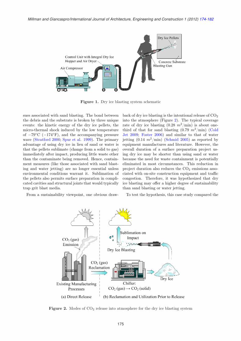
Millman and Giancaspro/International Journal of Architecture, Engineering and Construction 1 (2012) 174-182
Figure 1. Dry ice blasting system schematic
sues associated with sand blasting. The bond betweenthe debris and the substrate is broken by three uniqueevents: the kinetic energy of the dry ice pellets, themicro-thermal shock induced by the low temperatureof −79C (−174F), and the accompanying pressurewave (Stratford 2000; Spur et al. 1999). The primaryadvantage of using dry ice in lieu of sand or water isthat the pellets sublimate (change from a solid to gas)immediately after impact, producing little waste otherthan the contaminate being removed. Hence, contain-ment measures (like those associated with sand blast-ing and water jetting) are no longer essential unlessenvironmental conditions warrant it. Sublimation ofthe pellets also permits surface preparation in compli-cated cavities and structural joints that would typicallytrap grit blast media.
From a sustainability viewpoint, one obvious draw-
back of dry ice blasting is the intentional release of CO2
into the atmosphere (Figure 2). The typical coveragerate of dry ice blasting (0.28 m2/min) is about one-third of that for sand blasting (0.79 m2/min) (ColdJet 2009; Foster 2006) and similar to that of waterjetting (0.14 m2/min) (Schmid 2005) as reported byequipment manufactures and literature. However, theoverall duration of a surface preparation project us-ing dry ice may be shorter than using sand or waterbecause the need for waste containment is potentiallyeliminated in most circumstances. This reduction inproject duration also reduces the CO2 emissions asso-ciated with on-site construction equipment and trafficcongestion. Therefore, it was hypothesized that dryice blasting may offer a higher degree of sustainabilitythan sand blasting or water jetting.
To test the hypothesis, this case study compared the
Figure 2. Modes of CO2 release into atmosphere for the dry ice blasting system
175
Millman and Giancaspro/International Journal of Architecture, Engineering and Construction 1 (2012) 174-182
environmental effects of dry ice blasting, sand blast-ing, and water jetting by quantifying the environmen-tal impact of two key indicators, namely, CO2 emis-sions and fuel consumption. The assessment consideredthe commitment of environmental resources originatingfrom the construction staging area until the final dis-posal (end of construction activities) for a bridge repairproject undertaken in Rhode Island (USA). The anal-ysis consisted of (1) a baseline study to identify thevariables that had the most significant effect on theenvironment, and (2) a sensitivity analysis to examinethe variation of those critical variables identified in thebaseline study.
2 METHODOLOGY
To compare the processes, this case study analyzed abridge repair project undertaken in South Kingstown,Rhode Island (USA) (Giancaspro et al. 2009). The re-habilitation included the application of fiber-reinforcedpolymer (FRP) overlays to the reinforced concrete piercaps supporting the road deck of the Silver Spring CoveBridge. The substrate of the pier caps required appro-priate cleaning and surface abrasion (with water jet-ting) to allow for intimate contact between the parentsubstrate and composite overlay (ACI 2008). The dryice and sand blasting were conducted off-site for com-parison.The environmental assessment included three main
steps: goal definition and scoping, inventorying, andinterpretation. Goal definition and scoping were com-prised of defining the goals of the project, the type ofinformation that was needed, use/reuse/maintenance,the recycle/waste management protocol, and identify-ing the materials. The inventory required the devel-opment of a data collection plan, collecting data, andevaluating and documenting the results. The inter-pretation step included the identification of issues ofinterest, evaluating the completeness, sensitivity, andconsistency of the data, and drawing conclusions andrecommendations.This environmental assessment is not a Life Cycle
Assessment (LCA), a Life Cycle Inventory (LCI) nor aLife Cycle Impact Assessment (LCIA). A LCA encom-passes project start from the extraction of raw mate-rials from the earth continuing through the period ofuse up to the return of the materials back to the earth(end) (Curran 2006). The LCI is used to quantify theenergy and other discharges over the course of the lifecycle (Curran 2006). The LCIA is applied to evalu-ate the potential impact on humans’ health and theenvironment (Curran 2006).
2.1 Goal and Scope Definition
The goal of the case study was to determine underwhich conditions each surface preparation method (dryice blasting, sand blasting, or water jetting) performed
better in terms of CO2 emissions, fuel and energy con-sumption, and project duration.
Scope of the Study
The scope was to determine the most environmentallyconscious (with an equivalent mechanical effectiveness)substrate preparation and cleaning system. The func-tional unit was the Salt Pond Road Bridge rehabilita-tion project.
System Boundaries
The study covered the implementation processes of thethree systems and measured the energy required andCO2 emission from project start to end, and from con-struction staging area to the final disposal of the blast-ing media at the landfill or wastewater treatment plant.
Assumptions
The assumptions of the baseline study were based onequipment specifications, collected field data, and ap-proximations based on the authors’ experience. Theseincluded:
1. Near the construction zone, an imposed reduc-tion in vehicle speed of 64 to 32 km/h (40 to 20mph) created traffic congestion, which increasedfuel consumption and CO2 emissions.
2. To achieve the same degree of surface cleaning(aggressiveness), dry ice blasting and water jet-ting required longer dwell times (8.97 min/m2)and (7.18 min/m2), respectively, than sand blast-ing (4.45 min/m2); the equivalent blasting cov-erage rates were 0.11 m2/min, 0.14 m2/min, and0.22 m2/min, respectively.
3. Each pier cap was approximately 15.5 m (50.8ft) long with a surface area of 72.4 m2 (779 ft2)and supported seven prestressed concrete girders.The bridge consisted of two separate roadways -one for northbound traffic and another for south-bound traffic. Both pier caps were identical indesign.
4. A 2-lane principal arterial road passed beneaththe bridge and was parallel to the bridge columns.Rehabilitation activities in the designated con-struction zone created a 50% reduction in vehiclespeeds (congestion) from 64 to 32 km/h (40 to20 mph) over a 0.5 km (0.31 mile) stretch of theroad.
5. The average daily traffic flow on the principal ar-terial was taken as 4,250 vehicle/lane/day. Thiswas based on traffic data collected in 2008 by theFederal Highway Administration (FHWA 2008).
6. Each workday permitted 8 hours of work to beperformed; therefore, one-third of the daily traf-fic flow was affected by the reduced speed andcongestion, namely, 1,417 vehicles/lane/day.
176
Millman and Giancaspro/International Journal of Architecture, Engineering and Construction 1 (2012) 174-182
7. Approximately 2.35 kg of CO2 gas were releasedfor each liter, L, of gasoline a vehicle consumed(19.6 lb/gal) (Marland 2009; EPA 2009).
8. An additional 0.062 kg of CO2 was releasedper kilometer (0.221 lb/mile) per vehicle for theaforementioned reduction in speed. For the 0.5km (0.311 mile) stretch of road, this equated to0.031 kg (0.069 lb) (Barth and Boriboonsomsin2008).
9. Similar construction equipment (diesel-poweredgenerators and air compressors) of the same ca-pacity were used for all surface preparation meth-ods. Diesel fuel consumption was 2.27 L/h (0.60gal/h) (Diesel Service & Supply Inc. 2009).
10. Scaffolding setup and removal each required 2.3days per pier cap for each system (RSMeans2008).
11. The transportation modes and travel distancesof the materials (blasting media) from the con-struction staging area were identical and not con-sidered in terms of CO2 emission, fuel or energyconsumption, or project duration.
12. The travel distance of the waste byproducts tothe landfill or waste water treatment plant wasassumed negligible. Although sand blasting andwater jetting yielded more waste, the waste fromall methods was transported the same distance totheir end location (a landfill or wastewater treat-ment plant).
The assumptions specific to dry ice blasting included:
1. The dry ice blasting apparatus consumed 190 kg(427 lb) of dry ice per hour (Cold Jet 2012).
2. The blasting (or coverage) rate was 0.13 m2/min(1.4 ft2/min), which was based on actual mea-surements taken by the authors.
3. The blasting apparatus was estimated to con-sume approximately 0.0117 MW · h of en-ergy (Cold Jet 2012).
The assumptions relevant to sand blasting included:
1. In addition to scaffolding, sealed containment ar-eas to contain the blasting media and dust cloudwere constructed along the perimeter of the scaf-folding. Setup and removal each required 0.39days per pier cap (RSMeans 2001).
2. The coverage rate during blasting was 0.22 m2/min (2.4 ft2/min), which was based on actualmeasurements taken by the authors.
3. The blasting apparatus consumed 0 MW · h ofenergy (Kramer Industries 2009). The apparatusoperated using air pressure and did not requireadditional energy.
Assumptions specific to water jetting included:
1. The water blasting apparatus consumed 2,730 kg(6,000 lb) of water per hour (US Jetting, Inc.2012).
2. The blasting (or coverage) rate was 0.14 m2/min(1.5 ft2/min) (Schmid 2005).
3. The blasting apparatus was estimated to con-sume approximately 1.60 MW · h of energy (OJHøjtryk 2012).
2.2 Inventory Analysis
The system flow for the dry ice blasting process in-cluded the sublimation of pellets upon impact and theCO2 gas released into the atmosphere. The contam-inant shed from the substrate was transported to itsend location (landfill).The system flow for the sand blasting process began
with the sand propelled at the substrate using com-pressed air, then the mixture of waste and sand werecollected after use. The waste was transported to theend location for disposal.The system flow for the water jetting process began
with the water propelled at the substrate using com-pressed air, and the mixture of shed contaminant andwater were collected after use. The waste was trans-ported to the end location for disposal.For each system, the environmental effects were cat-
egorized into several project stages (or sources): sitesetup and deconstruction, equipment operation (us-age), vehicular traffic, media sublimation, and disposalof process wastes. More specifically:
1. The site setup and deconstruction included theerection and breakdown of scaffolding, setup andremoval of containment measures, and the re-moval of debris.
2. The equipment source included the fuel consump-tion and CO2 emissions from the equipment dur-ing the actual blast cleaning of the concrete sur-face. Since the blasting aggressiveness (ability toremove a layer of concrete with specified thick-ness) depended on the abrasive properties of theblasting media, the coverage rate (or dwell time)was varied.
3. The vehicular traffic source included the addi-tional CO2 emissions produced from vehicle traf-fic due to the project.
4. The media sublimation source was applicableonly to the dry ice blasting system and includedthe total CO2 emissions from media sublimation.
5. The disposal or process wastes stage included thecollection and transportation of waste to a land-fill.
2.3 Impact Assessment
The impact factors included project duration, CO2
emissions, and fuel and energy consumption. Theblasting process found to have the lesser values wasconsidered the process with the least environmentalimpact. Tables 1 and 2 show the CO2 emissions andenergy consumed by project stage, respectively.
177
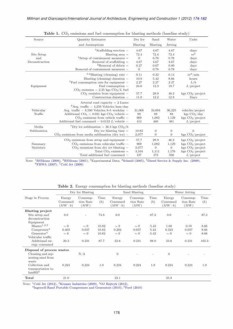
Millman and Giancaspro/International Journal of Architecture, Engineering and Construction 1 (2012) 174-182
Table 1. CO2 emissions and fuel consumption for blasting methods (baseline study)Source Quantity Estimates Dry Ice Sand Water Units
and Assumptions Blasting Blasting Jetting1Scaffolding erection = 4.67 4.67 4.67 days
Site Setup Blasting area = 72.4 72.4 72.4 m2
and 1Setup of containment measures = 0 0.78 0.78 daysDeconstruction Removal of scaffolding = 4.67 4.67 4.67 days
2Removal of debris = 0.27 0.67 0.80 daysRemoval of containment measures = 0 0.78 0.78 days
3,4Blasting (cleaning) rate = 0.11 0.22 0.14 m2/minBlasting (cleaning) duration = 10.8 5.42 8.66 hours
5Fuel consumption rate for equipment = 2.27 2.27 2.27 L/hEquipment Fuel consumption = 24.6 12.3 19.7 L/project
CO2 emission = 2.35 kgs CO2/L fuelCO2 emission from equipment = 57.7 28.9 46.2 kgs CO2/project
Construction duration = 11.0 12.2 12.8 Days
Arterial road capacity = 2 Lanes6Avg. traffic = 4,250 Vehicles/lane/day
Vehicular Avg. traffic = 8,500 Vehicles/8-h workday = 31,068 34,694 36,225 vehicles/projectTraffic Additional CO2 = 0.031 kgs CO2/vehicle = 88 88 88 kgs CO2/day
CO2 emissions from vehicle traffic = 969 1,082 1,129 kgs CO2/projectAdditional fuel consumed = 0.0133 L/vehicle = 412 460 481 L/project
Media 7Dry ice sublimation = 36.3 kgs CO2/h
Sublimation Dry ice blasting time = 10.82 0 0 hCO2 emissions from media sublimation (dry ice) = 2,077 0 0 kgs CO2/project
CO2 emissions from setup and equipment = 57.7 28.9 46.2 kgs CO2/projectSummary CO2 emissions from vehicular traffic = 969 1,082 1,129 kgs CO2/projectStatistics CO2 emissions from dry ice blasting = 2,077 0 0 kgs CO2/project
Total CO2 emissions = 3,104 1,111 1,176 kgs CO2/projectTotal additional fuel consumed = 437 473 500 L/project
Note: 1RSMeans (2008), 2RSMeans (2001), 3Experimental Data, 4Schmid (2005), 5Diesel Service & Supply Inc. (2009),6FHWA (2007), 7Cold Jet (2009)
Table 2. Energy consumption for blasting methods (baseline study)Dry Ice Blasting Sand Blasting Water Jetting
Stage in Process Energy Consump- Time Energy Consump- Time Energy Consump- TimeConsumed tion Rate (h) Consumed tion Rate (h) Consumed tion Rate (h)(MW · h) (MW ) (MW · h) (MW ) (MW · h) (MW )
Blasting projectSite setup and 0.0 - 74.8 0.0 - 87.2 0.0 - 87.2deconstructionEquipment
Blaster1,2,3 ∼ 0 ∼ 0 10.82 ∼ 0 ∼ 0 5.42 1.60 0.19 8.66Compressor4 0.403 0.037 10.82 0.202 0.037 5.42 0.323 0.037 8.66Generator4 ∼ 0 ∼ 0 10.82 ∼ 0 ∼ 0 5.42 ∼ 0 ∼ 0 8.66
Vehicular trafficAdditional en- 20.3 0.231 87.7 22.6 0.231 98.0 23.6 0.231 102.3ergy consumed
Disposal of process wastesCleaning and sep- N/A 0 - - 0 - -arating sand fromwasteCollection and 0.224 0.224 1.0 0.224 0.224 1.0 0.224 0.224 1.0transportation tolandfill5
Total 21.0 23.1 25.8
Note: 1Cold Jet (2012), 2Kramer Industries (2009), 3OJ Højtryk (2012),4Ingersoll-Rand Portable Compressors and Generators (2010), 5Ford (2010)
178
Millman and Giancaspro/International Journal of Architecture, Engineering and Construction 1 (2012) 174-182
3 DISCUSSION ANDINTERPRETATION
3.1 Baseline Case Study
Project Duration
Table 1 facilitates an equivalent comparison of the du-rations of the projects for the baseline study. The setupand removal of scaffolding required a total of 9.4 daysregardless of the blasting media employed. The actualsurface preparation (blasting) time using dry ice was10.8 hours, while that for sand blasting was 5.42 hoursand 8.66 hours for water jetting. Because the dry iceblasting was nearly twice as long as sand blasting, itmay seem that sand blasting was the faster method.However, this misconception can be disproven by com-paring the overall project durations of the methods.Sand blasting required 12.2 days, dry ice blasting re-quired 11.0 days, and water jetting required 12.8 days.Comparing the dry ice and sand, the difference of 1.2days was a 10.4% reduction in time for the scenarioemploying the dry ice. This significant savings in timestems from the 1.6 days needed for the combined setupand removal of containment measures, which was un-necessary for the dry ice blasting. Because the dry icesublimates, the overall project duration was reducedby 10.4% as compared to sand blasting, and by 14.3%as compared to water jetting. This reduction in timetranslated into reduced traffic delays and, hence, lessCO2 emissions from vehicular traffic.
CO2 Emissions
As shown in Table 1, the dry ice blasting scenario pro-duced 57.7 kg of CO2 from the setup and equipmentstages, 969 kg of CO2 from vehicular traffic, and 2,077kg of CO2 directly from blasting with dry ice (sub-limation) for a total of 3,104 kg. The sand blastingproject produced 28.9 kg of CO2 during the setup andequipment stage, and 1,082 kg of CO2 from vehicu-lar traffic, for a total of 1,111 kg. The water jettingproject produced 46.2 kg of CO2 during the setup andequipment stage, and 1,129 kg of CO2 from vehiculartraffic, for a total of 1,176 kg. Thus, the sand blast-ing released 1,993 kg less than that of dry ice blastingand 65 kg less than water jetting; this correspondedto reductions of 64.2% and 5.5%, respectively. Themajority of these reductions in CO2 for sand blastingstemmed from the blasting duration component. Thesand blasting cleaning rate was about double the ratesfor dry ice blasting or water jetting which allowed for afaster cleaning time and shorter blasting duration. Forthe sand blasting and water jetting scenarios, vehicu-lar traffic contributed the largest amount of the totalCO2 emissions as shown in Table 1 (31.2% for dry iceblasting, 97.4% for sand blasting, and 96.0% for waterjetting). Because the blasting duration overwhelminglygoverned the total CO2 emissions, the release of CO2
via dry ice sublimation was equitably significant.
Energy Consumption
The energy consumption analyses in Table 2 consid-ered the energy consumed on a system-wide perspec-tive, which included contributions from vehicular traf-fic. Energy consumption for dry ice blasting was 20.7MW · h during blasting, and 0.22 MW · h for disposal(total of 21.0 MW · h). For sand blasting and waterjetting, energy consumption was comparable to that ofdry ice for the disposal stage (0.22 MW ·h). However,the blasting stage (for sand) consumed 22.9 MW · h,which was 10.5% more energy than that consumed forthe dry ice. For water jetting, the blasting stage con-sumed 25.6 MW ·h, which was 23.6% more energy thanthat for dry ice. This difference in energy consump-tion was due to the longer project durations, which in-creased vehicular traffic for both the sand blasting andwater jetting systems. Additionally, the blasting appa-ratus of the equipment stage increased the total energyconsumption for the water jetting system. In terms ofthe total energy consumed, the dry ice scenario used21.0 MW · h whereas the sand blasting scenario used23.1 MW · h and the water jetting scenario used 25.8MW ·h. These differences equated to 10.0% and 23.2%less energy when using the dry ice blasting process.
Fuel Consumption
As expected, the reduction in vehicle speeds due to con-gestion increased the fuel consumption per vehicle. Forall systems, the assumed increase was 0.0133 L of fuelper vehicle, as shown in Table 1. Vehicles in the dry iceblasting system consumed an additional 437 L of fuelduring the project, while traffic for the sand blastingsystem consumed 8.2% more (total of 473 liters) andthe water jetting scenario consumed 14.4% more (totalof 500 liters).
3.2 Sensitivity Analyses
The results of the baseline study indicated that thevariable with the most significant environmental im-pact stemmed from traffic disruptions. To further ex-amine the sensitivity of this variable, two scenarioswere evaluated:
1. Scenario 1: variation of number of traffic lanesfrom 0 to 8 (Figure 3).
2. Scenario 2: variation of the average daily trafficflow from 0 to 12,000 vehicles/lane (Figure 4).
Scenario 1
The number of traffic lanes was varied from 0 to 8 lanes,though the average daily flow remained constant at4,250 vehicles/lane. Zero lanes of traffic correspondedto bridges that do not have roads passing beneaththem; thus, vehicular traffic would not be affected.For these bridges, the environmental effects from traf-fic disruptions were removed and the effect of dry icesublimation became more pronounced and significant.
179
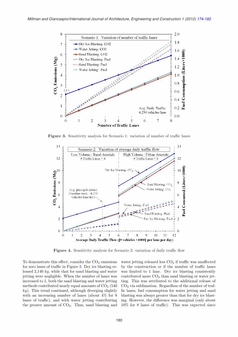
Millman and Giancaspro/International Journal of Architecture, Engineering and Construction 1 (2012) 174-182
Figure 3. Sensitivity analysis for Scenario 1: variation of number of traffic lanes
Figure 4. Sensitivity analysis for Scenario 2: variation of daily traffic flow
To demonstrate this effect, consider the CO2 emissionsfor zero lanes of traffic in Figure 3. Dry ice blasting re-leased 2,140 kg, while that for sand blasting and waterjetting were negligible. When the number of lanes wasincreased to 1, both the sand blasting and water jettingmethods contributed nearly equal amounts of CO2 (540kg). This trend continued, although diverging slightlywith an increasing number of lanes (about 4% for 8lanes of traffic), and with water jetting contributingthe greater amount of CO2. Thus, sand blasting and
water jetting released less CO2 if traffic was unaffectedby the construction or if the number of traffic laneswas limited to 1 lane. Dry ice blasting consistentlycontributed more CO2 than sand blasting or water jet-ting. This was attributed to the additional release ofCO2 via sublimation. Regardless of the number of traf-fic lanes, fuel consumption for water jetting and sandblasting was always greater than that for dry ice blast-ing. However, the difference was marginal (only about10% for 8 lanes of traffic). This was expected since
180
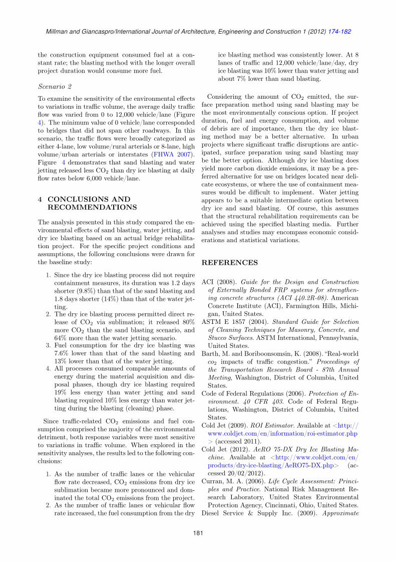
Millman and Giancaspro/International Journal of Architecture, Engineering and Construction 1 (2012) 174-182
the construction equipment consumed fuel at a con-stant rate; the blasting method with the longer overallproject duration would consume more fuel.
Scenario 2
To examine the sensitivity of the environmental effectsto variations in traffic volume, the average daily trafficflow was varied from 0 to 12,000 vehicle/lane (Figure4). The minimum value of 0 vehicle/lane correspondedto bridges that did not span other roadways. In thisscenario, the traffic flows were broadly categorized aseither 4-lane, low volume/rural arterials or 8-lane, highvolume/urban arterials or interstates (FHWA 2007).Figure 4 demonstrates that sand blasting and waterjetting released less CO2 than dry ice blasting at dailyflow rates below 6,000 vehicle/lane.
4 CONCLUSIONS ANDRECOMMENDATIONS
The analysis presented in this study compared the en-vironmental effects of sand blasting, water jetting, anddry ice blasting based on an actual bridge rehabilita-tion project. For the specific project conditions andassumptions, the following conclusions were drawn forthe baseline study:
1. Since the dry ice blasting process did not requirecontainment measures, its duration was 1.2 daysshorter (9.8%) than that of the sand blasting and1.8 days shorter (14%) than that of the water jet-ting.
2. The dry ice blasting process permitted direct re-lease of CO2 via sublimation; it released 80%more CO2 than the sand blasting scenario, and64% more than the water jetting scenario.
3. Fuel consumption for the dry ice blasting was7.6% lower than that of the sand blasting and13% lower than that of the water jetting.
4. All processes consumed comparable amounts ofenergy during the material acquisition and dis-posal phases, though dry ice blasting required19% less energy than water jetting and sandblasting required 10% less energy than water jet-ting during the blasting (cleaning) phase.
Since traffic-related CO2 emissions and fuel con-sumption comprised the majority of the environmentaldetriment, both response variables were most sensitiveto variations in traffic volume. When explored in thesensitivity analyses, the results led to the following con-clusions:
1. As the number of traffic lanes or the vehicularflow rate decreased, CO2 emissions from dry icesublimation became more pronounced and dom-inated the total CO2 emissions from the project.
2. As the number of traffic lanes or vehicular flowrate increased, the fuel consumption from the dry
ice blasting method was consistently lower. At 8lanes of traffic and 12,000 vehicle/lane/day, dryice blasting was 10% lower than water jetting andabout 7% lower than sand blasting.
Considering the amount of CO2 emitted, the sur-face preparation method using sand blasting may bethe most environmentally conscious option. If projectduration, fuel and energy consumption, and volumeof debris are of importance, then the dry ice blast-ing method may be a better alternative. In urbanprojects where significant traffic disruptions are antic-ipated, surface preparation using sand blasting maybe the better option. Although dry ice blasting doesyield more carbon dioxide emissions, it may be a pre-ferred alternative for use on bridges located near deli-cate ecosystems, or where the use of containment mea-sures would be difficult to implement. Water jettingappears to be a suitable intermediate option betweendry ice and sand blasting. Of course, this assumesthat the structural rehabilitation requirements can beachieved using the specified blasting media. Furtheranalyses and studies may encompass economic consid-erations and statistical variations.
REFERENCES
ACI (2008). Guide for the Design and Constructionof Externally Bonded FRP systems for strengthen-ing concrete structures (ACI 440.2R-08). AmericanConcrete Institute (ACI), Farmington Hills, Michi-gan, United States.
ASTM E 1857 (2004). Standard Guide for Selectionof Cleaning Techniques for Masonry, Concrete, andStucco Surfaces. ASTM International, Pennsylvania,United States.
Barth, M. and Boriboonsomsin, K. (2008). “Real-worldco2 impacts of traffic congestion.” Proceedings ofthe Transportation Research Board - 87th AnnualMeeting, Washington, District of Columbia, UnitedStates.
Code of Federal Regulations (2006). Protection of En-vironment. 40 CFR 403. Code of Federal Regu-lations, Washington, District of Columbia, UnitedStates.
Cold Jet (2009). ROI Estimator. Available at <http://www.coldjet.com/en/information/roi-estimator.php> (accessed 2011).
Cold Jet (2012). AeRO 75-DX Dry Ice Blasting Ma-chine. Available at <http://www.coldjet.com/en/products/dry-ice-blasting/AeRO75-DX.php> (ac-cessed 20/02/2012).
Curran, M. A. (2006). Life Cycle Assessment: Princi-ples and Practice. National Risk Management Re-search Laboratory, United States EnvironmentalProtection Agency, Cincinnati, Ohio, United States.
Diesel Service & Supply Inc. (2009). Approximate
181

Millman and Giancaspro/International Journal of Architecture, Engineering and Construction 1 (2012) 174-182
Fuel Consumption Chart. Available at <http://www.dieselserviceandsupply.com> (accessed 2011).
EPA (2009). Fuel Economy Guide 2009. Departmentof Energy, Environmental Protection Agency (EPA),United States.
FHWA (2007). Highway Statistics Series 2007, TableHM-62 - Weighted Average Daily Traffic Per Lane- 2007 on Principal Arterials. Federal HighwayAdministration (FHWA), Washington, District ofColumbia, United States. Available at <http://www.fhwa.dot.gov/policyinformation/statistics/2007/hm62.cfm> (accessed 2011).
FHWA (2008). Bridge Statistics for South Kingstown,Rhode Island (RI) - Condition, Traffic, Stress, Struc-tural Evaluation, Project Costs: National Bridge In-ventory (NBI) Statistics. Federal Highway Adminis-tration (FHWA), Washington, District of Columbia,United States.
Ford (2010). Ford Commercial Truck: F-450. Ford Commercial Truck. Available at<http://www.commtruck.ford.com/vehicle-specs.html?modelYearId=8902> (accessed 20/07/2012).
Foster, R. W. (2006). Carbon Dioxide (Dry-ice)Blasting. Available at <http://www.brothersindustrial.com> (accessed 13/07/2010).
Giancaspro, J., Papakonstantinou, C., Nazier, M.,and Balaguru, P. (2009). “Aerospace technology forstrengthening of bridges.” Construction and BuildingMaterials, 23(2), 748–757.
Ingersoll-Rand Portable Compressors and Generators(2010). Compressor HP915WCU. Ingersoll-RandPortable Compressors and Generators. Availableat <http://cfmpsiaircompressors.com/pdf/ingersoll-rand/675-1600.pdf> (accessed 20/09/2010).
Kramer Industries (2009). Heavy-Duty PortablePressure Blasting. Available at <http://www.kramerindustriesonline.com/blasting-systems/heavy-duty-ppb-series.htm>.
Mailvagnam, N. P., Pye, G. B., and Arnott, M. R.(1998). Surface Preparation of the Concrete Sub-strate. National Research Council of Canada: In-stitute for Research in Construction: ConstructionTechnology Update No. 24, Ottawa, Canada.
Marland, G. (2009). Carbon Dioxide Information Anal-
ysis Center. Oak Ridge National Laboratory, OakRidge, Tennessee, United States.
OJ Højtryk (2012). High Pressure Jetting Unit 225 ZP 24. Available at <http://www.oj-hojtryk.dk> (ac-cessed 22/02/2010).
Rosenberg, B., Yuan, L., and Fulmer, S. (2006). “Er-gonomics of abrasive blasting: A comparison of highpressure water and steel shot.” Applied Ergonomics,37(5), 659–667.
RSMeans (2001). RSMeans Heavy Construction CostData. RS Means Company, Kingston, Massachusetts,United States.
RSMeans (2008). RSMeans CostWorks. RS MeansCompany, Kingston, Massachusetts, UnitedStates. Available at <http://www.meanscostworks.com/securedsite/login.aspx> (accessed 2011).
Schmid, R. (2005). “Evolution of UHP waterjettingequipment: Surface preparation process found toyield higherproductivity than gritblasting.” MetalFinishing, 103(11), 41–60.
Spur, G., Uhlmann, E., and Elbing, F. (1999). “Dry-ice blasting for cleaning: process, optimization andapplication.” Wear, 233-235, 402–411.
Stout, D. (1996). Court Halts Sandblasting onBridges until Studies are Completed. The New YorkTimes. Available at <http://www.nytimes.com/1996/10/04/nyregion/court-halts-sandblasting-on-bridges-until-studies-are-completed.html>.
Stratford, S. (2000). “Dry ice blasting for paint strip-ping and surface preparation.” Metal Finishing,98(6), 493–499.
Teimourian, H., Shabgard, M., and Momber, A.(2010). “De-painting with high-speed water jets:Paint removal process and substrate surface rough-ness.” Progress in Organic Coatings, 69(4), 455–462.
US Jetting, Inc. (2012). US Jetting Industrial UnitJetters: US Jetting 5012 Electric High PresssureJetting Unit. US Jetting, Inc.. Available at <http://www.usjetting.com/electric-industrial.html> (ac-cessed 10/01/2012).
Weston, D. P., Shipway, P. H., and Harris, S. J. (2005).“Coating removal from an industrial polypropyleneblend by cryogenic blasting: The development ofsubstrate damage.” Wear, 258(1-4), 392–401.
182
International Journal of Architecture, Engineering and ConstructionVol 1, No 3, September 2012, 183-186
Book Review
David J. Kelly∗
School of Engineering Technology, College of Technology, Eastern Michigan University,
Ypsilanti, MI 48197, United States
Modern Construction: Lean Project Deliveryand Integrated Practices by Lincoln H. Forbesand Syed M. Ahmed. Boca Raton, FL: CRCPress. ISBN: 978-1-4200-6312-7.
DOI:10.7492/IJAEC.2012.020
Forbes and Ahmed have prepared an authoritative texton the emergent fields of lean construction and inte-grated practices [e.g., integrated project delivery (IPD)and building information modeling (BIM)]. While fre-quently presented (and studied) as separate and dis-tinct methods for improving performance outcomes,recent studies have shown that constructive synergiescan result from the integration of lean and various in-tegrated technologies (Sacks et al. 2010). Therefore,it is important and appropriate that these interrelatedtopics be presented together, in a single text. Prefacedby the authors as a tool to enhance productivity, thebook provides significant detail on the methods, ratio-nale, and historical justification for the implementationof lean and integrated technologies.
1 SCOPE AND SUBSTANCE
The book begins with a review of the constructionindustry. Focusing heavily on the need to improveproductivity and integration, the authors detail thestandard delivery methods and contract structures em-ployed by owners. Generally understood pros and consare presented, albeit with a noticeable emphasis on theshortcomings of traditional delivery methods and con-tract methodologies. Among the many industry prob-lems identified, a handful are congruent with thosefound by Rooke et al. (2004), i.e., the culture ofblame, exploitation, component optimization in lieu ofsystem optimization, and the pursuit of opportunis-tic claims. Performance and productivity measures inconstruction are presented, highlighting the role pro-ductivity plays in profit generation and the benefitsof improved productivity. Factors impacting construc-
tion productivity are detailed, including the roles ofmanagement, performance standards, subcontracting,innovation, and training. A brief discussion on earnedvalue analysis is included along with information onassessing percent completion and other similar projectbenchmarks.Mass production is contrasted with the Toyota Pro-
duction System (TPS) in a historical context, empha-sizing that the origins of lean theory reside in manufac-turing. The compatibility of lean with various emer-gent forms of relational contracting is discussed, as arethe shortcomings of traditional delivery methods, suchas design-bid-build. Through a presentation of leanconstruction fundamentals (e.g., customer focus, cul-ture, organization, waste elimination, continuous im-provement, and Five Big IdeasTM), the authors set thefoundation for a more detailed recitation of the toolsand techniques needed for a lean journey.An exhaustive presentation of prescriptive process
models, management devices, and general definitions-each marked with a simple acronym-are put forthas the means to both understand and implementlean construction theory. These include, but arenot limited to, the following: Lean Project DeliverySystemTM (LPDS); Last Planner SystemTM (LPS);weekly work plan (WWP); activity definition model(ADM); owner’s project requirements (OPR); post oc-cupancy evaluation (POE); target value design (TVD);plan, do, check, and act (PDCA); quality function de-ployment (QFD); percent planned complete (PPC);work in progress (WIP); reverse phase scheduling(RPS); Five-Step plan (5S); and rolled throughputyield (RTY). The discussion leaves the reader with afundamental understanding of the underlying premises,nomenclature, vocabulary, and apparatus of the leanconstruction movement.The text highlights the need for adequate training
and coaching in order to bring about the process andcultural adjustments necessary for successful imple-mentation of Lean practices. For example, within thediscussion of Just-in Time (JIT) delivery, the authors
*Email: [email protected]
183
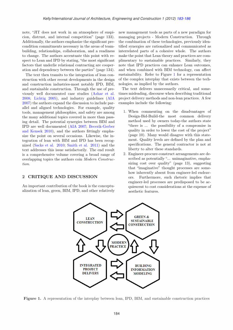
Kelly/International Journal of Architecture, Engineering and Construction 1 (2012) 183-186
note, “JIT does not work in an atmosphere of suspi-cion, distrust, and internal competition” (page 133).Additionally, the authors emphasize the significant pre-condition commitments necessary in the areas of team-building, relationships, collaboration, and a readinessto change. The authors accentuate this point with re-spect to Lean and IPD by stating, “the most significantfactors that underlie relational contracting are cooper-ation and dependency between the parties” (page 134).The text then transits to the integration of lean con-
struction with other recent developments in the designand construction industries-most notably IPD, BIM,and sustainable construction. Through the use of pre-viously well documented case studies (Azhar et al.2008; Lichtig 2005), and industry guidelines (AIA2007) the authors expand the discussion to include par-allel and aligned technologies. For example, qualitytools, management philosophies, and safety are amongthe many additional topics covered in more than pass-ing detail. The potential synergies between BIM andIPD are well documented (AIA 2007; Becerik-Gerberand Kensek 2010), and the authors fittingly empha-size the point on several occasions. Likewise, the in-tegration of lean with BIM and IPD has been recog-nized (Sacks et al. 2010; Smith et al. 2011) and thetext addresses this issue satisfactorily. The end resultis a comprehensive volume covering a broad range ofoverlapping topics the authors coin Modern Construc-tion.
2 CRITIQUE AND DISCUSSION
An important contribution of the book is the conceptu-alization of lean, green, BIM, IPD, and other relatively
new management tools as parts of a new paradigm formanaging projects - Modern Construction. Throughthe combination of these technologies, previously iden-tified synergies are rationalized and communicated asinterrelated parts of a cohesive whole. The authorsmake the point that Lean theory and practices are com-plimentary to sustainable practices. Similarly, theynote that IPD practices can enhance Lean outcomes,and when combined with BIM technology, can affectsustainability. Refer to Figure 1 for a representationof the complex interplay that exists between the tech-nologies, as implied by the authors.The text delivers unnecessarily critical, and some-
times misleading, discourse when describing traditionalproject delivery methods and non-lean practices. A fewexamples include the following:
1. When commenting on the disadvantages ofDesign-Bid-Build-the most common deliverymethod used by owners today-the authors state“there is ... the possibility of a compromise inquality in order to lower the cost of the project”(page 10). Many would disagree with this state-ment. Quality levels are defined by the plan andspecifications. The general contractor is not atliberty to alter these standards.
2. Engineer-procure-construct arrangements are de-scribed as potentially “... unimaginative, empha-sizing cost over quality” (page 13), suggestingthat “imaginative” thought processes are some-how inherently absent from engineer-led endeav-ors. Furthermore, such rhetoric implies thatengineer-led processes are predisposed to be ac-quiescent to cost considerations at the expense ofaesthetic features.
Figure 1. A representation of the interplay between lean, IPD, BIM, and sustainable construction practices
184
Kelly/International Journal of Architecture, Engineering and Construction 1 (2012) 183-186
3. Within the discussion of lessons learned it is as-serted that “project teams often start installa-tion of work packages too early, erecting incom-plete quantities of materials and equipment in adiscontinuous sequence because a certain amountof material happens to be on hand” (page 198).Such a broad generalization depicts pre-lean (tra-ditional) construction managers in an inaccurateand disparaging manner, as if such practitionersare unable or unwilling to properly schedule andsequence work flow in the absence of lean theoryand practice.
The cultural barriers to widespread adoption of Mod-ern practices are formidable (AIA 2007; Ghassemi andBecerik-Gerber 2011; Rooke et al. 2004). Most propo-nents of Modern practices - the authors included - failto emphasize or recognize the significant barriers thatare entrenched within the industry landscape (e.g., in-stitutional, cultural, technical, and contractual). Gen-erational turn-over may be required to see the imple-mentation of the models and practices proposed in thetext. Similarly, the effort required to learn and adoptthe specialized vernacular of lean construction is notdiscussed as a potential impediment to implementa-tion.While the text includes a brief note on the 14
Points and Seven Deadly Diseases put forth by Deming(1982), a robust discussion of Deming’s enormous con-tribution in the areas of lean thought, statistical pro-cess control, industrial management, and the TPS is ashortcoming. The authors repeatedly focus on maxi-mizing the whole and not the part, they do not addressthe challenges associated with the inherently diffuse na-ture of building construction work. A typical buildingproject may have hundreds of subcontractors and sup-pliers contracted at multiple levels. Even in the caseof an IPD tri-party arrangement, many of these sec-ond and third tier entities will remain unaffected as aresult of the adoption of Modern practices by manage-ment and select 1st tier contractors. This conundrumleaves one to question how the adoption of these princi-ples and practices can significantly improve productiv-ity on a measurable project-wide basis. This conditionis exacerbated by the varied nature of subcontracting.At times, the authors assume that subcontractors andsuppliers are willing to learn a new way of behaving forthe benefit of one project, only to become equally adeptat abandoning the integrated mindset when moving totheir next (presumably traditional) project.The span of topical coverage is broad. In addition
to covering anticipated subject matter suggested bythe title (e.g., lean construction, IPD, BIM, and sus-tainability), the authors extend the content of the textto include reviews of affiliated issues including perfor-mance improvement, construction safety management,workforce management, and systems integration. Al-though the aim of such inclusiveness is admirable, stu-dious, and well intentioned, its effect on the standing of
the text is debatable. A case in point is the narrative onnoise in the construction environment, where the au-thors state, “ . . . sounds can distract workers from doingwhat they are supposed to do” (page 385). Althoughthis statement may be absolutely true, noise and audi-tory distractions are largely unavoidable byproducts ofthe process of building construction-especially for thestructural and framing trades. Such discourse couldleave readers wondering from what perspective the au-thors were writing.
3 CONCLUSION
The text is a compendium of the latest research andthinking on lean and integrated practices. By integrat-ing and contextualizing the current thinking on a widevariety of construction management practices, the au-thors have prepared a useful and dependable resourcefor both academicians and industry professionals alike.While the tone of a portion of the commentary doesappear biased, it does not substantially detract fromthe value of the work. Equally, the extended coveragesections (e.g., safety, work force management, perfor-mance improvement, and systems integration) are notcritical to the delivery of the main thrust of the text,but do provide useful background and contextual un-derpinning for the central themes of the work. Prac-tical matters of adoption and industry evolution couldbe discussed in more detail. Should a second editionbe planned in the future, the critique contained hereinmay provide useful material for updating and expand-ing the text.
REFERENCES
AIA (2007). Integrated project delivery: a guide.American Institute of Architects (AIA) CaliforniaCouncil. Available at < http://www.aia.org/contractdocs/AIAS077630> (accessed 01/05/2011).
Azhar, S., Hein, M., and Sketo, B. (2008). “Build-ing information modeling: Benefits, risks and chal-lenge.” 44th annual international conference of theassociated schools of construction, Auburn Univer-sity, Auburn, Alabama, United States.
Becerik-Gerber, B. and Kensek, K. (2010). “Buildinginformation modeling in architecture, engineering,and construction: Emerging research directions andtrends.” Journal of Professional Issues in Engineer-ing Education and Practice, 136(3), 139–147.
Deming, W. E. (1982). Out of the Crisis. MIT Centerfor Educational Services, Cambridge, Massachusetts,United States.
Ghassemi, R. and Becerik-Gerber, B. (2011). “Transi-tioning to integrated project delivery: Potential bar-riers and lessons learned.” Lean Construction Jour-nal, 32–52.
Lichtig, W. A. (2005). “Sutter health: Developing a
185

Kelly/International Journal of Architecture, Engineering and Construction 1 (2012) 183-186
contracting model to support lean project delivery.”Lean Construction Journal, 2(1), 105–112.
Rooke, J., Seymour, D., and Fellows, R. (2004). “Plan-ning for claims: an ethnography of industry culture.”Construction Management and Economics, 22(6),655–662.
Sacks, R., Koskela, L., Dave, B., and Owen, R. (2010).
“Interaction of lean and building information model-ing in construction.” Journal of Construction Engi-neering and Management, 136(9), 968–980.
Smith, R. E., Mossman, A., and Emmitt, S. (2011).“Editorial: Lean and integrated project delivery spe-cial issue.” Lean Construction Journal, 1–16.
186