NGET Process Appendix

To accompany Issue 16

2

VERSION CONTROL

VERSION HISTORY

Date Version Comments

28/04/17 1 Submission

3

TABLE OF CONTENTS

Version Control ....................................................................................................................................................... 2

Version History ................................................................................................................................................... 2

Glossary .................................................................................................................................................................. 5

Purpose of Process Appendix ................................................................................................................................. 6

Appendix Overview................................................................................................................................................. 7

Asset (A) (1.1.1.) ................................................................................................................................................. 7

Material Failure Mode (F) (1.1.2.) ...................................................................................................................... 7

Probability of Failure P(F) (1.1.3.) ...................................................................................................................... 7

Event (E) (1.1.5.) ................................................................................................................................................. 8

Probability of Event P(E) (1.1.6) ......................................................................................................................... 8

Asset Risk (1.1.7.) ............................................................................................................................................... 8

Network Risk (3.5.) ............................................................................................................................................. 9

Risk is Modelled at an Asset Level .................................................................................................................... 10

Assets transition from a functional to a failed state ........................................................................................ 10

FMEA identifies relevant failure modes ........................................................................................................... 11

Failure Curves are generated from the parameters supplied in the FMEA ..................................................... 11

Probability of Material Failure ......................................................................................................................... 12

Treatment of Inspection and Detection (1.1.4) .................................................................................................... 14

Conceptual model ............................................................................................................................................ 14

Probability of Failure (2.) ...................................................................................................................................... 15

Process for FMEA (2.1) ..................................................................................................................................... 15

Failure Modes (2.2.) ......................................................................................................................................... 17

Detecting Potential to Functional Failure Modes ........................................................................................ 17

Detecting Utilisation Failure Modes ............................................................................................................ 17

Detecting Random Failure Modes ............................................................................................................... 17

Probability of Failure (2.3.) ............................................................................................................................... 18

Deriving Parameters for Probability Distributions ....................................................................................... 18

Mapping End of Life Modifier to Probability of Failure (2.3.2.) ................................................................... 19

4

Calculating Probability of Failure (2.3.3.) ..................................................................................................... 23

Forecasting Probability of Failure (2.3.4.) .................................................................................................... 24

Determining End of Life Modifier ................................................................................................................ 25

Implementation PLan ........................................................................................................................................... 52

Data Collection for EOL Modifier Parameters .................................................................................................. 52

Assumptions ......................................................................................................................................................... 53

Uncertainty (4.3.) .................................................................................................................................................. 65

Requirements ................................................................................................................................................... 65

Model Developed To Specifically Address Requirements ................................................................................ 66

Monte Carlo Simulation Is Used To Generate Cis For The Expected Number Of Events ................................. 67

Analytical Techniques and Monte Carlo Are Used to Generate Network Risk with Cis ................................... 68

Estimating Uncertainty in Input Data - EOL Modifier ....................................................................................... 69

Stage A ......................................................................................................................................................... 70

Stage B ......................................................................................................................................................... 70

Stage C ......................................................................................................................................................... 71

Applying the methodology........................................................................................................................... 71

Risk Trading Model ............................................................................................................................................... 72

Requirements ................................................................................................................................................... 72

Implementation ................................................................................................................................................ 73

5

GLOSSARY

Term Definition

Condition Inspection

An inspection which provides information on the state of an asset

which is including in the calculations for probability of failure.

An inspection can be both Remedial and Condition.

Constant Failure Mode A failure mode with a constant rate of failure irrespective of age or

time since last intervention.

EOL Modifier

End of Life Modifier incorporates condition information for an asset

generating an effective age which is used to generate a probability of

failure.

Event Something which can happen as a result of a failure mode and has a

monetised consequence associated with it.

Failure Curve The cumulative probability density function generated for a particular

failure mode using parameters supplied in the FMEA.

Failure Mode

A distinct way in which an asset or a component may fail. Fail means it

no longer does what is designed to do and has a significant probability

of causing a material consequence. Each failure mode needs to be

mapped to one or more failure mode events.

Increasing Failure Mode A failure mode which has an increasing probability of occurring over

time.

Lead Asset

One of the following:

1. Circuit Breakers

2. Transformers

3. Reactors

4. Underground Cable

5. Overhead Lines

a. Conductor

b. Fittings

Monetised Consequence

The cost to the transmission system of a particular event occurring.

Broken into non-overlapping types: Financial, Safety, Environment,

System.

NGET National Grid Electricity Transmission

NOMs Network Output Measures

Random Failure Mode A failure mode with a constant rate of failure irrespective of age or

time since last intervention.

Remedial Action Action taken on finding a failure and before the asset is required to

operate.

Remedial Inspection

An inspection, like an operational test, which tests whether an asset is

functioning. If the asset isn’t functioning action is taken to either

remove the asset from the system or repair the functional failure.

An inspection can be both Remedial and Condition.

6

PURPOSE OF PROCESS APPENDIX

Ofgem has requested modifications to the existing RIIO methodology to better facilitate achievement of the

NOMs objectives. The current method assigns condition scores and criticality categories to assets, aiming to

ensure the distribution of scores and criticalities remains within acceptable bounds. The required method is

one where the probability of failure for an asset is understood, together with a monetised consequence of

failure. This generates a risk score which can be aggregated across the network to yield Network Risk.

This document explains the NGET Risk Methodology developed to meet this objective and how specific

requirements contained in Ofgem’s ‘Direction to Modify NOMs Methodology’ will be delivered.

In developing the methodology, NGET has borne the following Ofgem guidance in mind:

“The Methodology shall be designed to facilitate the NOMs Objectives and to comply with the principles of

transparency and objectivity as described below:

Transparency - the Methodology should contain sufficient detail to explain to a competent independent

assessor why and how investments are prioritised and how efficient levels of past and future expenditure

are determined. The publicly available elements of the NOMs should enable a competent reader without

access to sensitive information or data to form a theoretical view on performance of a ‘Generic TO’1.

Objectivity - the Methodology will be unambiguous and enable any two competent independent assessors

(with access to the same input data) to arrive at the same view of licensees’ performance (over- delivery,

under-delivery, or on target delivery) and to identify and quantify the relevant factors contributing to

performance.”

In addition, the team developing the methodology within NGET have worked to the following guiding

principles:

The “system” provides a consistent response – Distinct assets of the same type in an identical state and

located within equivalent network topologies should generate equal monetised risk scores. The term

“system” refers not only to the model but to the end to end process of collecting data, making any

assumptions, using the model and interpreting results.

Is able to improve over time with new data – Our understanding of assets and how they deteriorate, due

environmental conditions, usage or time, is continuously improving. A suitable methodology must be

flexible enough to incorporate future knowledge making better predictions in a transparent and auditable

manner.

As simple as required but not simpler – when choosing between simple and more complicated

approaches we have chosen the simpler approach. Except where a more complex approach demonstrably

improves predictive power.

Distil engineering experience and judgement from across NGET – Within NGET we have access to many

decades of globally recognised technical knowledge and experience. During the development process we

have spoken to and incorporated feedback from respected engineers and asset managers.

Use proven engineering and mathematical techniques –The FMEA methodology and the use of standard

statistical techniques for modelling reliability are proven and have a long track record in electricity

transmission and across many industries.

7

APPENDIX OVERVIEW

ASSET (A) (1.1.1.)

An asset is defined as a unique instance of one of the five types of lead assets:

1. Circuit Breakers

2. Transformers

3. Reactors

4. Underground Cable

5. Overhead Lines

a. Conductor

b. Fittings

Overhead Line and Cable routes are broken down into appropriate segments of the route. Each Asset belongs

to an Asset Family. An Asset Family has one or more material Failure Modes. A material Failure Mode can lead

to one or more Events.

MATERIAL FAILURE MODE (F) (1.1.2.)

The failure mode is a distinct way in which an asset or a component may fail. Fail means it no longer does what

is designed to do and has a significant probability of causing an Event with a monetised consequence. Each

failure mode needs to be mapped to one or more Events.

Each failure mode (Fi) needs to be mapped to one or more Events (Ej) and the conditional probability the Event

will manifest should the failure occur P(Ej|Fi).

PROBABILITY OF FAILURE P(F) (1.1.3.)

Probability of failure (P(Fi)) represents the probability that a Failure Mode will occur in the next time period. It

is given by:

𝑷(𝑭𝒊) = 𝑺𝒕 − 𝑺𝒕+𝟏

𝑺𝒕

Equation 1

𝑤ℎ𝑒𝑟𝑒:

𝑃(𝐹𝑖) = 𝑡ℎ𝑒 𝑝𝑟𝑜𝑏𝑎𝑏𝑖𝑙𝑖𝑡𝑦 𝑜𝑓 𝑓𝑎𝑖𝑙𝑢𝑟𝑒 𝑚𝑜𝑑𝑒 𝑖 𝑜𝑐𝑐𝑢𝑟𝑟𝑖𝑛𝑔 𝑑𝑢𝑟𝑖𝑛𝑔 𝑡ℎ𝑒 𝑛𝑒𝑥𝑡 𝑡𝑖𝑚𝑒 𝑖𝑛𝑡𝑒𝑟𝑣𝑎𝑙

𝑆𝑡 = 𝑡ℎ𝑒 𝑐𝑢𝑚𝑢𝑙𝑎𝑡𝑖𝑣𝑒 𝑝𝑟𝑜𝑏𝑎𝑏𝑖𝑙𝑖𝑡𝑦 𝑜𝑓 𝑠𝑢𝑟𝑣𝑖𝑣𝑎𝑙 𝑢𝑛𝑡𝑖𝑙 𝑡𝑖𝑚𝑒 𝑡

𝑆𝑡+1 = 𝑡ℎ𝑒 𝑐𝑢𝑚𝑢𝑙𝑎𝑡𝑖𝑣𝑒 𝑝𝑟𝑜𝑏𝑎𝑏𝑖𝑙𝑖𝑡𝑦 𝑜𝑓 𝑠𝑢𝑟𝑣𝑖𝑣𝑎𝑙 𝑢𝑛𝑡𝑖𝑙 𝑡𝑖𝑚𝑒 𝑡 + 1

It is generated from an underlying parametric probability distribution or failure curve, taking into account any

remedial inspections. The nature of this curve and its parameters (i.e. increasing or random failure rate,

earliest and latest onset of failure) are provided FMEA. The probability of failure is influenced by a number of

factors, including time, duty and condition.

8

EVENT (E) (1.1.5.)

The monetised value for each of the underlying Financial, Safety, System and Environmental components of a

particular event e.g. Transformer Fire. Each Ej has one or more Fi mapped to it. An Event can be caused by

more than one Failure Mode, but an Event itself can only occur once during the next time period. For example,

an Asset or a particular component is only irreparably damaged once.

PROBABILITY OF EVENT P(E) (1.1.6)

If Event j can be caused by n failure modes, then P(Ej) the probability of event j occurring in the next time

interval is given by:

𝑷(𝑬𝒋) = 𝟏 − ∏(𝟏 − 𝑷(𝐌𝑭𝒊

𝒎

𝒊=𝟏

) × 𝑷(𝑬𝒋|𝑭𝐢)

Equation 2

𝑤ℎ𝑒𝑟𝑒:

𝑃(𝐸𝑗) = 𝑃𝑟𝑜𝑏𝑎𝑏𝑖𝑙𝑖𝑡𝑦 𝑜𝑓 𝐸𝑣𝑒𝑛𝑡 𝑗 𝑜𝑐𝑐𝑢𝑟𝑟𝑖𝑛𝑔 𝑑𝑢𝑟𝑖𝑛𝑔 𝑎 𝑔𝑖𝑣𝑒𝑛 𝑡𝑖𝑚𝑒 𝑝𝑒𝑟𝑖𝑜𝑑

𝑃(𝑀𝐹𝑖) = 𝑃𝑟𝑜𝑏𝑎𝑏𝑖𝑙𝑖𝑡𝑦 𝑜𝑓 𝑚𝑎𝑡𝑒𝑟𝑖𝑎𝑙 𝑓𝑎𝑖𝑙𝑢𝑟𝑒 𝑚𝑜𝑑𝑒 𝑖 𝑜𝑐𝑐𝑢𝑟𝑟𝑖𝑛𝑔 𝑑𝑢𝑟𝑖𝑛𝑔 𝑡ℎ𝑒 𝑛𝑒𝑥𝑡 𝑡𝑖𝑚𝑒 𝑖𝑛𝑡𝑒𝑟𝑣𝑎𝑙

𝑃(𝐸𝑗|𝐹𝑖) = 𝐶𝑜𝑛𝑑𝑖𝑡𝑖𝑜𝑛𝑎𝑙 𝑝𝑟𝑜𝑏𝑎𝑏𝑖𝑙𝑖𝑡𝑦 𝑜𝑓 𝐸𝑣𝑒𝑛𝑡 𝑗𝑔𝑖𝑣𝑒𝑛 𝐹𝑖 ℎ𝑎𝑠 𝑜𝑐𝑐𝑢𝑟𝑒𝑑

The derivation of 𝑃(𝑀𝐹𝑖) from 𝑃(𝐹𝑖)is explained in section Error! Reference source not found. as part of t

reatment of inspection and detection.

ASSET RISK (1.1.7.)

For a given asset (Ak), a measure of the risk associated with it is the Asset Risk, given by:

𝑨𝒔𝒔𝒆𝒕 𝑹𝒊𝒔𝒌(𝑨𝒌) = ∑𝑷(𝑬𝒋)

𝒏

𝒋=𝟏

× 𝑬𝒋

Equation 3

𝑤ℎ𝑒𝑟𝑒:

𝑃(𝐸𝑗) = 𝑃𝑟𝑜𝑏𝑎𝑏𝑖𝑙𝑖𝑡𝑦 𝑜𝑓 𝐸𝑣𝑒𝑛𝑡 j 𝑜𝑐𝑐𝑢𝑟𝑟𝑖𝑛𝑔 𝑑𝑢𝑟𝑖𝑛𝑔 𝑎 𝑔𝑖𝑣𝑒𝑛 𝑡𝑖𝑚𝑒 𝑝𝑒𝑟𝑖𝑜𝑑

𝐸𝑗 = 𝑡ℎ𝑒 𝑚𝑜𝑛𝑒𝑡𝑖𝑠𝑒𝑑 𝐸𝑣𝑒𝑛𝑡 𝑗

𝑛 = 𝑡ℎ𝑒 𝑛𝑢𝑚𝑏𝑒𝑟 𝑜𝑓 𝐸𝑣𝑒𝑛𝑡𝑠 𝑎𝑠𝑠𝑜𝑐𝑖𝑎𝑡𝑒𝑑 𝑤𝑖𝑡ℎ 𝐴𝑠𝑠𝑒𝑡 𝑘

9

NETWORK RISK (3.5.)

Network Risk is the sum of individual Asset Risks and is given by:

𝑵𝒆𝒕𝒘𝒐𝒓𝒌 𝑹𝒊𝒔𝒌(𝑵𝑹) = ∑𝑨𝒌

𝒎

𝒌=𝟏

Equation 4

𝑤ℎ𝑒𝑟𝑒:

𝐴𝑘 = 𝐴𝑠𝑠𝑒𝑡 𝑅𝑖𝑠𝑘 𝑓𝑜𝑟 𝑎𝑠𝑠𝑒𝑡 𝑘

10

RISK IS MODELLED AT AN ASSET LEVEL

We calculate Risk at an Asset level, assuming asset failures are independent, this allows aggregation and

comparison of risk across geography and asset type.

• Asset failures are independent of other Assets.

• Failure modes for a particular asset are

independent

• Events given a failure mode are not

independent – the same event can arise through

different failure modes

• The model does not include circuit and

network information

• Asset specific system consequences act as a

proxy for this information

ASSETS TRANSITION FROM A FUNCTIONAL TO A FAILED STATE

Assets transition from a functional to a failed state via Failure Modes. Material failure modes can lead to

Events which have monetised Consequences..

Network

SGT OHLCB

R1 R2 Rn

A1 AnA2

Region

Type

Asset

Figure 2 An SGT has many failure modes which can lead to a Tx fire. A fire is an Event with a monetised consequence.

Figure 1

11

FMEA IDENTIFIES RELEVANT FAILURE MODES

The FMEA process identifies failure modes, interventions which address them and provides the parameters

required to generate a probabilistic model. Interventions for particular Failure Modes are identified during the

FMEA process.

Figure 3

FAILURE CURVES ARE GENERATED FROM THE PARAMETERS SUPPLIED IN THE FMEA

The FMEA process specifies the nature of particular failure modes, for example if it’s increasing or random,

whether any inspection or condition information can be used to update the effective age of an asset.

Figure 4

Transformers, Bushing

Cat 1

Events Interventions

FMEA_Family Item Failure Mode F S E R Insp. Basic InterM MajorRefur

b

Repla

ceDGA Pattern Earliest Latest

Tap Changer Tapchanger Selector 9 yrs fail to operate 3 4 1 1 0 0 0 1 0 0 0 Increasing 9 12

Transformer Cooling System reduced cooling capacity 1 1 1 3 1 1 0 1 0 0 0 Increasing 3 11

QB Cooling System reduced cooling capacity 1 1 1 3 1 1 0 1 0 0 0 Increasing 3 11

1. Increasing FMs* are modelled using a Weibull curve

2. The parameters for the curve are determined by using

data supplied in the FMEA to fit the eqn. below.

3. The curve can then be used to

generate PoFs

12

PROBABILITY OF MATERIAL FAILURE

A failure is only material1 if it occurs before an asset is required to operate and both occur before the next

maintenance or replacement intervention. We are interested in P(F<T)P(E<T|E>Tf), where:

T denotes the time until next intervention,

F time to failure,

E the time until the failed functionality is required to by the asset to operate.

Figure 5

Periodic tests or operations can spot failures before an asset is required to operate, therefore reducing the

probability of a material event.

1 Doesn’t lead to an Event(E) but will still require repair

Failure

Asset Operates

1st M Interval

Material Failure

Failure

Asset Operates

1st M Interval2nd M Interval

Not A Material Failure

Failure

Asset Operates

1st M Interval

Periodic Test

Periodic Tests reduce P(Material Failure)

13

In general the probability of material failure in any given year is given by:

𝑷(𝑴𝒂𝒕𝒆𝒓𝒊𝒂𝒍 𝑭𝒂𝒊𝒍𝒖𝒓𝒆) = (∑ 𝒑𝒒𝒌−𝟏𝒛𝒏𝒎−𝒌𝒏×𝒎

𝒌=𝟏

) × (𝟏 − 𝒛𝒎) + ∑𝒑𝒒𝒌−𝟏(𝟏 − 𝒛𝒏−𝒌)

𝒎

𝒌=𝟏

Equation 5

𝑤ℎ𝑒𝑟𝑒:

𝑛 = 𝑦𝑒𝑎𝑟𝑠 𝑠𝑖𝑛𝑐𝑒 𝑙𝑎𝑠𝑡 𝑖𝑛𝑠𝑝𝑒𝑐𝑡𝑖𝑜𝑛, 𝑖𝑛𝑡𝑒𝑟𝑣𝑒𝑛𝑡𝑖𝑜𝑛 𝑜𝑟 𝑟𝑒𝑝𝑎𝑖𝑟

𝑚 = 𝑛𝑢𝑚𝑏𝑒𝑟 𝑜𝑓 𝑠𝑢𝑏 − 𝑖𝑛𝑡𝑒𝑟𝑣𝑎𝑙𝑠 𝑜𝑓 𝑎 𝑦𝑒𝑎𝑟2

𝑝 = 𝑝𝑟𝑜𝑏𝑎𝑏𝑖𝑙𝑖𝑡𝑦 𝑜𝑓 𝑓𝑎𝑖𝑙𝑢𝑟𝑒 𝑖𝑛 𝑟𝑒𝑙𝑒𝑣𝑎𝑛𝑡 𝑠𝑢𝑏 𝑖𝑛𝑡𝑒𝑟𝑣𝑎𝑙

𝑞 = 1 − 𝑝

𝑦 = 𝑝𝑟𝑜𝑏𝑎𝑏𝑖𝑙𝑖𝑡𝑦 𝑜𝑓 𝑎𝑠𝑠𝑒𝑡 𝑜𝑝𝑒𝑟𝑎𝑡𝑖𝑛𝑔 𝑖𝑛 𝑠𝑢𝑏 − 𝑖𝑛𝑡𝑒𝑟𝑣𝑎𝑙

𝑧 = 1 − 𝑦

When assets are annually inspected the above equation simplifies to:

𝑷(𝑴𝒂𝒕𝒆𝒓𝒊𝒂𝒍 𝑭𝒂𝒊𝒍𝒖𝒓𝒆) =∑𝒑𝒒𝒌−𝟏(𝟏 − 𝒛𝒏−𝒌)

𝒎

𝒌=𝟏

Equation 6

since immediately after an inspection 𝑛 = 0.

When a failure mode immediately results in an Event then P(Failure) and P(Material Failure) are equal.

By treating inspections like this we can estimate the inspection frequency required to maintain a given

P(Material Failure) as an asset ages and maintain mitigated risk. This also sets the lower bounds of a

continuous monitoring system which is not to the rate of inspection but the time taken to complete a remedial

action.

2 for example we can break a year into 365 days so m = 365. The shorter the sub-interval, the greater run time.

14

TREATMENT OF INSPECTION AND DETECTION (1.1.4)

CONCEPTUAL MODEL

Two separate aspects of Inspections effect the outcome of the model in different ways. Inspections provide

condition information which can be used to generate a more accurate P(Failure) and/or check if an asset is

working as expected at time of the inspection (in the form of operational tests).

Operational tests or inspections reduce the probability of material Events if Action is taken when a defect is

identified and before the Asset is required to function on the network.

Figure 7

For example a CB may have a hidden drive train fault which means it will not operate when required to break a

fault current. This would be a significant event but a remedial inspection would uncover the hidden failure

allowing it to be repaired before a potentially catastrophic event.

50 OK

50 Failed

N = 100

P(E) = 0.5

50 OK

5 Failed

45 Failed

Inspection

95% Effective

Action

(Fix or Replace)

50 OK

45 New

5 Failed

N = 100

P(E) = 0.05

D

G

A

D

G

A

Today

P(F)

Historic inspections provide condition

information to

incorporate into P(F) calculations

Future inspections reduce P(E|F) as they

are an opportunity to

detect a failure and act before a material

Event.

PastFuture

Figure 6 - Inspections provide condition infomation and an opportunity to fix hidden failures.

15

PROBABILITY OF FAILURE (2.)

PROCESS FOR FMEA (2.1)

The process for identifying failure modes uses component studies for each asset class to understand the asset

risk.

For each component, each failure mode (that is each component) is assessed to determine:

Detection: effectiveness of detection, where applicable

Event: all possible events including the probability of a particular event. It is connected with each

failure mode, whichever type that failure mode may be

Probability of Failure

Type of Failure Mode (P-F, utilisation, random)

For the purpose of calculating Asset Risk, the FMEA process generates the following outputs by Asset Type:

List of significant failure modes both within life and at end of life

Identification of interventions which address each failure mode

Potential events should a failure mode occur and the likelihood of the event occurring given the

failure mode

The financial, safety, environment and reliability consequences resulting from the event

Classification of a failure mode as time based, duty or random (or a combination)

For increasing time based failure modes expected earliest (2.5% of the population) and latest onset of

failure (97.5% of the population) and the most appropriate underlying density function (Weibull, bi-

normal) since installation or the latest relevant intervention

For random failure modes, the random rate of failure. These are known failure modes and are

expressed as a % failures per year

Inspections which aim to detect potential failures before they occur, their likelihood of success and

their period of validity

An internal procedure (TP237) has been written for FMEA which is kept confidentially in the Licnsee Specific

Appenidx for NGET.

16

Figure 8

Output comparable to expected

failures?

INITIAL FMEA (TP237 Process)

Lead assets

RISK MODEL

REVIEW OUTPUT FOR EACH ASSET CLASS

FAULTS/FAILURES/DEFECTS/ACU

1. STAGED REVIEW OF FMEA a. Revise Probability of Failure

(earliest/latest onset or constant failure rate)

b. Revise P(Event) of Failure Modes

2. STAGED DEVELOPMENT OF RISK MODEL

c. Incorporate maintenance plans (current) to understand

impact of interventiond. Incorporate inspection

plans/routines to understand detection

FURTHER ITERATIONS OF FMEA /

DEVELOPMENT OF RISK MODEL

N

Y

Identify Asset Items

Identify failure modes for each asset item

Determine means and effectiveness of detection

Identify all events resulting from failure mode.

Identify Available interventions

Understand the type of failure mode and the

probability of that failure mode occurrence

Identify Modifiers and Differentiators for Location

and Environment

Understand whether a triggering event will affect the asset’s probability of

failure

Determine Probability of Failure and Probability of

Event (Risk Model)

17

FAILURE MODES (2.2.)

FMEA takes into account the effectiveness of the detection technique, determined as a percentage, as not all

failure modes will result in 100% detection from the inspection technique. Indeed for some failure modes,

effective detection is technically not possible or economically unviable.

DETECTING POTENTIAL TO FUNCTIONAL FAILURE MODES

As this failure mode is time based, the detection method will only be valid for a certain duration following the

detection activity, i.e. the risk is reduced for a fixed time period and then increases until the next inspection or

intervention.

DETECTING UTILISATION FAILURE MODES

These failure modes are based upon the utilisation of particular assets. For example, the deterioration of

assets such as circuit breakers is based upon the number of operations it carries out. It is possible to forecast

the expected duty for individual assets and hence interventions can be planned before the risk increases above

a specified limit.

DETECTING RANDOM FAILURE MODES

By definition these failure modes are difficult to detect until the failure actually happens. Forensic analysis of

failed assets or components can provide valuable information about the failure mode and its future detection

the interventions that could prevent it.

18

PROBABILITY OF FAILURE (2.3.)

The process illustrated below will be used to determine the probability of failure of each asset. In particular we

will need to translate from the end of life modifier that will be determined in the subsequent sections. This will

be done by translating through a probability mapping step, so that the appropriate end of life curve can be

used to determine the probability of an asset having failed.

DERIVING PARAMETERS FOR PROBABILITY DISTRIBUTIONS

The failure modes and effects analysis defined an end of life curve for each asset family. It is recognised that

some of these predicted deterioration mechanisms have yet to present themselves and were based on

knowledge of asset design and specific R&D into deterioration mechanisms. In summary the following sources

of data were utilised:

Results of forensic evidence

Results of condition assessment tests.

Results of continuous monitoring

Historical and projected environmental performance (e.g. oil loss)

Historical and projected unreliability

Defect history for that circuit breaker family.

19

The end of life failure curve will be based in terms of the data points corresponding to the ages at which 2.5%,

and 97.5% of failures occur. The method for determining the end of life curves was explained in the failure

modes and effects analysis section of this document.

Typically within each lead asset group there will be separate end of life curves determined for each family

grouping. Assignment to particular family groupings is through identification of similar life limiting factors.

MAPPING END OF LIFE MODIFIER TO PROBABILITY OF FAILURE (2.3.2.)

Each lead asset within the NOMs risk model has an end of life failure modifier score. These scores need to be

translated to a probability on the relevant failure mode curve. This end of life probability of failure (PoF) is

determined from the end of life (EOL) modifier, which itself is determined from the asset’s current condition,

duty, age and asset family information. The EOL modifier has been developed to have a strong relationship

with the likelihood of asset failure but is not itself a PoF over the next year.

A probability mapping function is required to enable mapping from an EOL modifier to a conditional PoF. The

figure below illustrates distributions representing the end of life failure mode for a population of transformer.

The 50% point on the cumulative distribution function (green) indicates the anticipated asset life (AAL). The

conditional PoF at the AAL can be determined from the red curve in the figure below (approximately 10% per

year). We can use this as an initial value in the mapping function, such that an EOL modifier of 100 is

equivalent to a 10% conditional PoF.

PoF can’t be utilised at an individual asset level to infer individual asset risk, and therefore the PoF values need

to be aggregated across the asset population in order to support the calculation of risk. Over a population of

assets at a given a PoF we have an expectation of how this PoF will continue to deteriorate over time, duty or

condition. This is shown by the conditional PoF curve in red.

Figure 9

20

The development of a methodology that maps the EOL modifier to PoF needs to consider the actual number of

failures that we experience, it should then be validated against the expected population survival curve and it

should satisfy the following requirements:

High scoring young assets should be replaced before low scoring old assets. The mapping function

achieves this objective because high scoring assets will always reach their AAL quicker than those of

low scoring assets.

When two assets of similar criticality have the same EOL modifier score then the older asset should be

replaced first. The mapping function will assign the same PoF to both assets, so they reach their

respective AAL at the same time. In practice the planner could prioritise the older asset for

replacement over the younger asset without penalty.

When an asset is not replaced the PoF should increase. The EOL modifier score reflects the condition

of the asset, and will therefore increase over time. This means the PoF will also increase.

A comprehensive and steady replacement programme will lead to a stabilisation of the population’s

average PoF. The proposed methodology will satisfy this requirement as worsening PoF would be

offset by replacements.

The PoF and resulting risks must be useful for replacement planning. The proposed methodology is

validated against the expected survival function, so should be compatible with existing replacement

planning strategies.

Outputs should match observed population data. The expected survival function for the population is

already identified based on known asset deterioration profiles and transmission owner experience.

The mapping to PoF method is validated against this expected population statistic.

In the following example we will consider how the conditional mapping function is derived for a transformer,

and then how the mapping curve parameters can be systematically adjusted through a process of validation

and calibration against the expected population’s survival curve.

The mapping function is given by the following exponential function.

𝐶𝑜𝑛𝑑𝑖𝑡𝑖𝑜𝑛𝑎𝑙 𝑃𝑜𝐹 = exp (𝑘 ∗ 𝐸𝑂𝐿𝑚𝑜𝑑𝛼) – 1

Equation 7

The parameter 𝛼 is tuned so that the deterioration profile over the population is consistent with the expected

survival function for the relevant population of assets. The expected survival function is given by the FMEA

earliest and latest onset of failure values, which have been determined though the transmission owner

experience using all available information such as manufacturer data and understanding of asset design.

The parameter k scaling value ensures that for an EOL modifier score of 100 the expected conditional PoF is

obtained (given as 𝛽 in the formula below). The formula is given by:

𝑘 = 𝑙𝑛 (1 + 𝛽

100𝛼)

Equation 8

The PoF mapping function is shown in the figure below for a transformer with 𝛼=1.7 and 𝛽=10%.

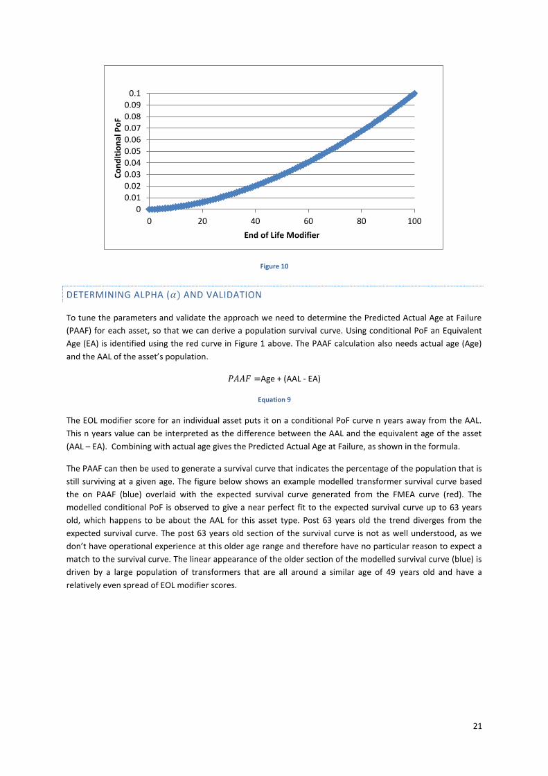
21

Figure 10

DETERMINING ALPHA (𝛼) AND VALIDATION

To tune the parameters and validate the approach we need to determine the Predicted Actual Age at Failure

(PAAF) for each asset, so that we can derive a population survival curve. Using conditional PoF an Equivalent

Age (EA) is identified using the red curve in Figure 1 above. The PAAF calculation also needs actual age (Age)

and the AAL of the asset’s population.

𝑃𝐴𝐴𝐹 =Age + (AAL - EA)

Equation 9

The EOL modifier score for an individual asset puts it on a conditional PoF curve n years away from the AAL.

This n years value can be interpreted as the difference between the AAL and the equivalent age of the asset

(AAL – EA). Combining with actual age gives the Predicted Actual Age at Failure, as shown in the formula.

The PAAF can then be used to generate a survival curve that indicates the percentage of the population that is

still surviving at a given age. The figure below shows an example modelled transformer survival curve based

the on PAAF (blue) overlaid with the expected survival curve generated from the FMEA curve (red). The

modelled conditional PoF is observed to give a near perfect fit to the expected survival curve up to 63 years

old, which happens to be about the AAL for this asset type. Post 63 years old the trend diverges from the

expected survival curve. The post 63 years old section of the survival curve is not as well understood, as we

don’t have operational experience at this older age range and therefore have no particular reason to expect a

match to the survival curve. The linear appearance of the older section of the modelled survival curve (blue) is

driven by a large population of transformers that are all around a similar age of 49 years old and have a

relatively even spread of EOL modifier scores.

0

0.01

0.02

0.03

0.04

0.05

0.06

0.07

0.08

0.09

0.1

0 20 40 60 80 100

Co

nd

itio

nal

Po

F

End of Life Modifier

22

Figure 11

DETERMINING BETA (𝛽) AND VALIDATION

Beta (𝛽) sets the maximum conditional PoF which would be expected for an asset that has reached its AAL. As

described in the earlier section an initial value can be determined from the FMEA end of life failure curve

earliest and latest onset values. A value of 10% was chosen for transformers, although there is a scope to tune

this value using failure data. The total PoF across the population can be obtained by summing the individual

conditional PoFs; this is then compared to the observed failures noting that many assets are replaced before

they fail. In the case of transformers the sum of conditional PoF gives 5 transformer failures per year. Each

year we actually experience 2 transformer failures, but replace 16. It therefore seems reasonable that if we

didn’t replace these 16 transformers then we might experience 5 failures each year. The value for 𝛽 can be

tuned such that the number of failures is similar to what is actually observed, but any tuning needs to be

performed in conjunction with the parameter 𝛼.

The parameters alpha (𝛼) and beta (𝛽) are both calibrated by considering population level statistics. In the

same sense the PoF or risk is only meaningful when aggregated across the asset population.

OIL CIRCUIT BREAKER CONDITIONAL POF MAPPING EXAMPLE

The analysis described above was repeated for Oil Circuit Breaker (OCB) EOL modifier scoring data in order to

validate and quantify the proposed method against expectation based on transmission owner experience. We

map the EOL modifier values to a conditional PoF using a similar function to that shown in Figure 1 above,

noting that the value of 𝛼 and 𝛽 will be specific to this OCB asset type. For the purpose of implementing this

methodology we assume that the conditional PoF is 𝛽=10% per year for an EOL modifier score of 100. We also

assume an initial value of 𝛼 that will be adjusted.

Using the same method described above for transformers we determine PAAF for each OCB on the network.

Plotting these PAAF values as a survival curve, overlaid with the expected survival curve, allows us to quantify

the model against expected asset deterioration and provides a mechanism for tuning the mapping parameter

𝛼. The modelled survival curve shown in the figure below has been produced with 𝛼=2.1 and 𝛽=10%. The

model follows the expected survival curve of OCBs across the life of the asset.

23

Figure 12

CALCULATING PROBABILITY OF FAILURE (2.3.3.)

As described above the probability of failure curve is based in terms of two data points that correspond to the

ages at which specific proportions of the asset’s population is expected to have failed. Using these data points

we can construct a cumulative distribution function F(t). The survival function is given as: S(t) = 1-F(t). The

conditional probability of failure is then given by the following formula, where t is equivalent age in the case of

end of life failure modes:

𝑃𝑜𝐹(𝑡) =𝑆(𝑡) − 𝑆(𝑡 + 1)

𝑆(𝑡)

Equation 10

In order to calculate the end of life probability of failure associated with a given asset, the asset will need to be

assigned an end of life modifier. This end of life modifier is derived from values such as age, duty and condition

information where it is available. In the absence of any condition information age is used. The service

experience of assets of the same design and forensic examination of decommissioned assets may also be taken

into account when assigning an end of life modifier. Using the end of life modifier we can then determine an

asset’s equivalent age and then map onto a specific point on the probability of failure curve.

The generalised end of life modifier (EOLmod) formula has the following structure for assets that have

underlying issues that can be summed together:

𝐸𝑂𝐿𝑚𝑜𝑑 = ∑ 𝐶𝑖

𝑛𝑢𝑚𝑏𝑒𝑟 𝑜𝑓𝑐𝑜𝑚𝑝𝑜𝑛𝑒𝑛𝑡𝑠

𝑖=1

Equation 11

Or for transformer assets that are single assets with parallel and independent failure modes the following

generalised end of life modifier formula is used:

24

𝐸𝑂𝐿𝑚𝑜𝑑 =

(

1 − ∏ (1 −

𝐶𝑖𝐶𝑚𝑎𝑥

)

𝑛𝑢𝑚𝑏𝑒𝑟 𝑜𝑓𝑐𝑜𝑚𝑝𝑜𝑛𝑒𝑛𝑡𝑠

𝑖=1

)

∗ 100

Equation 12

Ci represents an individual component parameter of the end of life modifier

Cmax represents the max score that the component can get

For some of the lead asset types the generalised formula will need to be nested to derive an overall asset end

of life modifier. For example in the case of OHLs we need to take the maximum of the preliminary end of life

modifier and a secondary end of life modifier.

The end of life modifier will range from zero to 100, where 100 represents the worst health that an asset could

be assigned. It is then necessary to convert the end of life modifier to a probability of failure to enable

meaningful comparison across asset types.

As far as reasonably possible the scores assigned to components of the end of life modifier are set such that

they are comparable e.g. are on the same magnitude. This enables the end of life modifier between different

assets in the same family to be treated as equivalent. The magnitude and relative difference between scores is

set using expert to judgement as there is limited data available. The validation and testing of these scores is

described in the testing section of the Common Methodology.

FORECASTING PROBABILITY OF FAILURE (2.3.4.)

Where appropriate and enough historical data exists, a rate multiplier can be applied, so that for each annual

time step in forecast time equivalent age is increased or decreased by the rate multiplier time step. The

default value of the rate multiplier time step is set as 1.0 per year. This modelling feature will allow high duty

assets to be forecast more accurately.

25

DETERMINING END OF LIFE MODIFIER

CIRCUIT BREAKER PARAMETERS

SCORING PROCESS

Circuit breakers will be assigned an end of life modifier according to the formula below. The maximum of the

two components as shown is determined, and it is capped at 100.

𝐸𝑂𝐿𝑚𝑜𝑑 = max (𝐴𝐺𝐸_𝐹𝐴𝐶𝑇𝑂𝑅, 𝐷𝑈𝑇𝑌_𝐹𝐴𝐶𝑇𝑂𝑅, 𝑆𝐹6_𝐹𝐴𝐶𝑇𝑂𝑅 )

Equation 13

The EOL modifier is therefore determined based on the maximum of its constituent parts. AGE_FACTOR,

DUTY_FACTOR, and SF6_FACTOR are non-dimensional variables with possible values between 0 and 100.

𝐴𝐺𝐸_𝐹𝐴𝐶𝑇𝑂𝑅 = C1 × FSDP ×Age

𝐴𝐴𝐿

Equation 14

Age: Reporting year - Installation year (years)

C1: a scaling factor to convert Age to a value in the range 0 to 100. The method for calculating C1 is

described at the end of this section

AAL is the anticipated asset life determined through FMEA analysis. The end of life curve described in

the Failure Modes and Affects analysis section can be used to determine AAL, which is the 50% point

on the respective end of life failure mode curve. The process for deriving these failure mode curves,

which we use to determine AAL, are themselves estimated using historical data and engineering

judgement. Further explanation is available in the section of this methodology discussing FMEA

FSDP is a family specific deterioration correction function described below. This is a function

multiplier to convert AGE from a linear function to an exponential function. This has the effect of

decreasing the relative significance of lower values of AGE

DUTY_FACTOR

The duty of each circuit breaker asset is determined using the following formula:

𝐷𝑈𝑇𝑌_𝐹𝐴𝐶𝑇𝑂𝑅 = C1 × 𝐹𝑆𝐷𝑃 × max (((𝑂𝐶)

(𝑀𝑂𝐶)) , (

(𝐹𝐶)

(𝑀𝐹𝐶)))

Equation 15

Where:

OC is the current asset operational count

MOC is the expected max asset operational count over a lifetime. For older circuit breakers this is

determined through liaison with suppliers, and for newer circuit breakers this is determined during

type testing

FC is the current accumulated fault current

26

MFC is the max permissible fault current over a lifetime. The value for MFC is set to 80% of the value

of the maximum rated value for the asset

FC and MFC are determined through liaison with suppliers who confirm operational limits for the mechanism

and interrupter.

Note that the DUTY_FACTOR has been normalised to account for variations in the asset life of the circuit

breaker family. This normalisation means that the end of life modifier of a circuit breaker from one family can

be compared to the end of life modifier of a circuit breaker from a different family. Age and other duty related

metrics are important due to the lack of more specific condition information.

FAMILY SPECIFIC DETERIORATION PROFILE (FSDP)

The Family Specific Deterioration profile accounts for the expected deterioration of an asset. This is needed as

there is limited availability of Asset Specific condition information. This function is based on duty value D which

is given by the following formula:

𝐷 = max (𝑂𝐶

𝑀𝑂𝐶,𝐹𝐶

𝑀𝐹𝐶,𝐴𝐺𝐸

𝐴𝐴𝐿)

Equation 16

The family specific deterioration function is determined using the function:

𝐹𝑆𝐷𝑃 = 𝑒𝑘∗𝐷2− 1

Equation 17

This parameter k is determined such that when D=1.0 then FSDP=1.0. This gives a value of k=0.694. FSDP is

capped at 1.0.

This function ensures that the impact of family specific deterioration is correctly considered in the health score

formula.

Figure 13

0

0.1

0.2

0.3

0.4

0.5

0.6

0.7

0.8

0.9

1

0 0.2 0.4 0.6 0.8 1 1.2

FSD

P -

Co

rre

ctio

n v

alu

e

D

27

The curve will generate a value from 0 to 1 depending on the duty of the asset. This curve is used within this

method due to the lack of condition information, and allows us to accelerate or suppress duty values

depending on the deterioration we would expect for that asset family. Note that while the shape of the curve

is fixed, the duty value (D) captures family specific factors such as anticipated asset life, maximum fault current

and maximum number of operations.

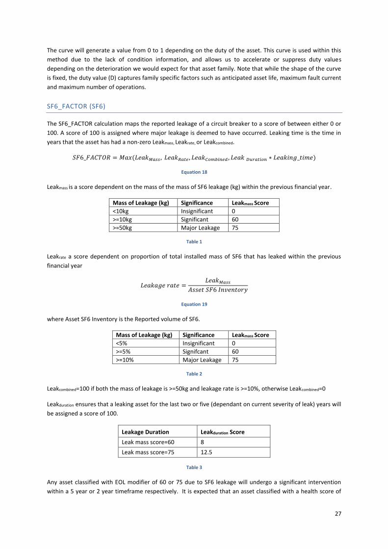
SF6_FACTOR (SF6)

The SF6_FACTOR calculation maps the reported leakage of a circuit breaker to a score of between either 0 or

100. A score of 100 is assigned where major leakage is deemed to have occurred. Leaking time is the time in

years that the asset has had a non-zero Leakmass, Leakrate, or Leakcombined.

𝑆𝐹6_𝐹𝐴𝐶𝑇𝑂𝑅 = 𝑀𝑎𝑥(𝐿𝑒𝑎𝑘𝑀𝑎𝑠𝑠 , 𝐿𝑒𝑎𝑘𝑅𝑎𝑡𝑒 , 𝐿𝑒𝑎𝑘𝐶𝑜𝑚𝑏𝑖𝑛𝑒𝑑 , 𝐿𝑒𝑎𝑘 𝐷𝑢𝑟𝑎𝑡𝑖𝑜𝑛 ∗ 𝐿𝑒𝑎𝑘𝑖𝑛𝑔_𝑡𝑖𝑚𝑒)

Equation 18

Leakmass is a score dependent on the mass of the mass of SF6 leakage (kg) within the previous financial year.

Mass of Leakage (kg) Significance Leakmass Score

<10kg Insignificant 0

>=10kg Significant 60

>=50kg Major Leakage 75

Table 1

Leakrate a score dependent on proportion of total installed mass of SF6 that has leaked within the previous

financial year

𝐿𝑒𝑎𝑘𝑎𝑔𝑒 𝑟𝑎𝑡𝑒 =𝐿𝑒𝑎𝑘𝑀𝑎𝑠𝑠

𝐴𝑠𝑠𝑒𝑡 𝑆𝐹6 𝐼𝑛𝑣𝑒𝑛𝑡𝑜𝑟𝑦

Equation 19

where Asset SF6 Inventory is the Reported volume of SF6.

Mass of Leakage (kg) Significance Leakmass Score

<5% Insignificant 0

>=5% Signifcant 60

>=10% Major Leakage 75

Table 2

Leakcombined=100 if both the mass of leakage is >=50kg and leakage rate is >=10%, otherwise Leakcombined=0

Leakduration ensures that a leaking asset for the last two or five (dependant on current severity of leak) years will

be assigned a score of 100.

Leakage Duration Leakduration Score

Leak mass score=60 8

Leak mass score=75 12.5

Table 3

Any asset classified with EOL modifier of 60 or 75 due to SF6 leakage will undergo a significant intervention

within a 5 year or 2 year timeframe respectively. It is expected that an asset classified with a health score of

28

75 today will reach a health score of 100 within 2 years, which has been set-up to reflect legislation that

significant SF6 leakers should be repaired within 2 years. The decision over which type of intervention to carry

out, whether that is repair, reconditioning, refurbishment or replacement, will be cost justified for the expected

benefit to the consumer. This means that risk will be reduced through the most cost justified intervention,

which may not necessarily be asset replacement.

Whilst there are pre-existing technologies that exist to carry out minor repairs to stop SF6 leaks, analysis of

these repairs demonstrates that in the majority of instances they are temporary in nature and a further major

intervention is then required to permanently repair the asset.

Broadly there are two functional requirements for a Gas Circuit Breaker. Firstly it must be able to break load,

and secondly it must be able to retain the Insulating Medium. This is based on the requirements described in

the Fluorinated Greenhouse Gases Regulations 2015, which places significant limits on permitted Leakage.

1. Operators of equipment that contains fluorinated greenhouse gases shall take precautions to prevent

the unintentional release (‘leakage’) of those gases. They shall take all measures which are technically

and economically feasible to minimise leakage of fluorinated greenhouse gases.

2. Where a leakage of fluorinated greenhouse gases is detected, the operators shall ensure that the

equipment is repaired without undue delay. (Chapter 2 Article 3 Sections 2 and 3 from http://eur-

lex.europa.eu/legal-content/EN/TXT/PDF/?uri=CELEX:32014R0517&from=EN)

29

PROCEDURE FOR DETERMINING C1

This value of this parameter is determined by calculating a value for EOL modifier from historical switchgear

data. The C1 value is tuned so that a reasonable translation between historical AHI’s, which were calculated

under the previous RIIO-T1 volume based methodology, and EOL modifier is achieved. Assets that were classed

as AHI1 previously should normally have a score of 100 under the new methodology. This approach is

consistent with the theme of the direction, as it enables a translation from previously classified AHI’s.

Based on this approach the parameter is fixed as 𝐶1 = 5/6.

EOL MODIFIER CALCULATION EXAMPLE

The following table shows three assets with example data that will allow us to determine the EOL modifier

Component Example Asset 1 Example Asset 2 Example Asset 3

Asset Operation Count (OC) 350 3000 350

Max Asset Operation Count (MOC) 5000 5000 5000

Accumulated Fault Current (FC) 400 400 1000

Max Permissible Fault Current (MFC) 1400 1400 1400

Anticipated Asset Life (AAL) 45 45 45

SF6 leakage (kg) 2 10 1

Age 40 20 15

Table 4

Applying the relevant formula presented in the above sections yields the following output.

Example Asset 1 Example Asset 2 Example Asset 3

D (in FSDP) 0.89 0.6 0.71

FSDP 0.72 0.28 0.41

AGE_FACTOR 53.19 10.23 11.23

DUTY_FACTOR 16.73 13.94 24.16

SF6_FACTOR 0 60 0

EOL Modifier 53.2 60 24.2

Table 5

The EOL Modifier in example asset 1 is driven by age factor, example 2 is driven by SF6 factor and example 3 is

driven by the duty factor (in particular the accumulated fault current).

The EOL modifier calculation proposed here facilitates a reasonable translation from the AHI’s utilised within

the existing RIIO-T1 methodology. An initial validation has been performed to calculate EOL modifier over a

range of assets and then comparing to the AHI determined under the existing methodology.

It should be noted that placing a cap on the age related components of health score would substantially impair

the translation from the previous AHI to health score.

30

TRANSFORMER AND REACTOR PARAMETERS

SCORING PROCESS

The scoring process needs to takes account of the three failure modes – dielectric, mechanical and thermal as

well as issues with other components that may significantly impact the remaining service life. The end of life

modifier is determined according to the following formula:

𝐸𝑂𝐿𝑚𝑜𝑑 = (1 − (1 −𝐷𝐶𝐹

100) (1 −

𝑇𝐶𝐹

100) (1 −

𝑀𝐶𝐹

100) (1 −

𝑂𝐶𝐹

100)) ∗ 100

Equation 20

The components of the end of life modifier are assigned using the scoring system described below. The

component OCF (other component factor) is a factor that accounts for other issues that can affect transformer

end of life. The maximum value of EOLmod is 100.

DIELECTRIC CONDITION FACTOR (DCF)

Dielectric condition is assessed using dissolved gas analysis (DGA) results. The score can be increased if the

indication is that the individual transformer is following a trend to failure already seen in other members of

the family. Where it is known that the indications of partial discharge are coming from a fault that will not

ultimately lead to failure e.g. a loose magnetic shield then the score may be moderated to reflect this but the

possibility of this masking other faults also needs to be taken into account.

Score Dielectric Condition Factor (DCF)

0 All test results normal: no trace of acetylene; normal levels of other gases and no

indication of problems from electrical tests.

2 Small trace of acetylene in main tank DGA or stray gassing as an artefact of oil type,

processing or additives. Not thought to be an indication of a problem.

10 Dormant or intermittent arcing/sparking or partial discharge fault in main tank.

30 Steady arcing/sparking or partial discharge fault in main tank.

60 Indications that arcing/sparking fault is getting worse.

100 Severe arcing/sparking or partial discharge fault in main tank – likely to lead to

imminent failure.

Table 6

THERMAL CONDITION FACTOR (TCF)

Thermal condition is assessed using trends in DGA and levels of furans in oil, . Individual Furfural (FFA) results

are unreliable because they can be influenced by temperature, contamination, moisture content and oil top

ups, therefore a trend needs to be established over a period of time. The presence of 2 Furfural (2FAL) is

usually required to validate the FFA result and the presence or absence of methanol is now being used to

31

validate (or otherwise) conclusions on thermal score. Thermal condition is understood to include ageing and

older, more heavily used and/or poorly cooled transformers tend to have higher scores. The score can be

increased if the indication is that the individual transformer is following a trend to failure already seen in other

members of the family.

Score Thermal Condition Factor (TCF)

0

No signs of ageing including no credible furans >0.10ppm and methanol ≤0.05ppm.

The credibility of furan results usually depends on the presence of 2 Furfural

(2FAL).

2

Diagnostic markers exist that could indicate ageing (including credible furans in the

range 0.10-0.50ppm) but are either not showing a credible progression or are

thought to be the result of contamination.

The credibility of furan results usually depends on the presence of 2 Furfural

(2FAL).

10

Indications or expectations that the transformer is reaching or has reached mid-life

for example: credible furans in the range 0.51-1.00ppm or stable furans >1ppm

possibly as a result of historic ageing.

and/or

Raised levels of methane or ethane in main tank DGA consistent with low

temperature overheating.

and/or

Transformers with diagnostic markers resulting from oil contamination (e.g. furans,

specifically 2FAL) that may mask signs of ageing.

30

Moderate ageing for example: credible furans consistently > 1ppm with a clear

upward trend.

and/or

Significant overheating fault (steadily rising trend of ethylene in main tank DGA).

60

Advanced ageing for example: credible furans > 1.5ppm showing a clear upward

trend or following the indications of a sister unit found to be severely aged when

scrapped.

and/or

Indications of a worsening overheating fault.

100

Very advanced ageing for example: credible furans >2ppm with an upward trend or

following the indications of a sister unit found to be severely aged when scrapped.

and/or

Serious overheating fault.

Table 7

Electrical test data may be used to support a higher thermal score where they show poor insulation condition.

Electrical tests can provide further evidence to support the asset management plan for individual transformers

e.g. where a significant number of oil tops ups have been required for a particularly leaky transformer and it is

suspected that this is diluting the detectable Furans in the oil. However experience shows that not all poor

thermal conditions can be detected by electrical tests which is why DGA data remains the focus for scoring the

Thermal Condition Factor.

32

MECHANICAL CONDITION FACTOR (MCF)

Mechanical condition is assessed using Frequency Response Analysis (FRA) results.

Score Mechanical Condition Factor (MCF)

0 No known problems following testing.

1 No information available.

3

Anomalous FRA results at the last measurement which are suspected to be a

measurement problem and not an indication of mechanical damage.

and/or

Corrected loose clamping which may reoccur.

10 Loose clamping.

30 Suspected mechanical damage to windings. This does not include cases where

the damage is confirmed.

60 Loose or damaged clamping likely to undermine the short circuit withstand

strength of the transformer.

100 Confirmed mechanical damage to windings.

Table 8

Mechanical condition is assessed using Frequency Response Analysis (FRA) results; FRA is used to detect

movement in the windings of the transformer, these data are supplemented by family history e.g. where post

mortem analysis of a similar transformer has confirmed winding movement and DGA results (which indicate

gas generation from loose clamping) as appropriate.

OTHER COMPONENT FACTOR (OCF)

The Other Components score uses an assessment of other aspects, this includes:

Tap-changers. Tap-changers are maintained and repaired separately to the transformer and defects

are most likely repairable therefore tap-changer condition does not normally contribute to the AHI

score. Where there is a serious defect in the tap-changer and it cannot be economically repaired or

replaced this will be captured here.

Oil Leaks. During the condition assessment process transformers may be found to be in a poor

external condition (e.g. severe oil leaks), this will be noted and the defect dealt with as part of the

Asset Health process. The severity of oil leaks can be verified by oil top up data. Where there is a

serious defect and it cannot be economically repaired, this will be captured here.

Other conditions such as tank corrosion, excessive noise or vibration that cannot be economically

repaired will be captured here.

33

Score Other Component Factor (OCF)

0 No known problems.

10

Leaks (in excess of 2000 litres per annum) that cannot be economically repaired.

and/or

Tap-changer that is known to be obsolete and spare parts are difficult to acquire.

30

Exceptional cases of leaking (in excess of 10 000 litres per annum) that cannot be

economically repaired where the annual oil top up volume is likely to be diluting

diagnostic markers.

and/or

Other mechanical aspects potentially affecting operation that cannot be

economically repaired for example: tank corrosion, excessive noise or vibration.

60

Exceptional cases of leaking (in excess of 15 000 litres per annum) that cannot be

economically repaired and where the effectiveness of the secondary oil

containment system is in doubt and would be difficult or impossible to repair

without removing the transformer.

and/or

Tap-changer that is known to be in poor condition and obsolete with no spare

parts available.

100 Confirmed serious defect in the tap-changer that cannot be economically

repaired or replaced.

Table 9

34

UNDERGROUND CABLE PARAMETERS

SCORING PROCESS

The formula to determine the EOL modifier for cables, which is capped at a maximum of 100, is:

𝐸𝑂𝐿𝑚𝑜𝑑 = 𝐴𝐶𝑆 + 𝑆𝑢𝑏_𝐴𝐷𝐽

Equation 21

Where ACS is the main asset condition score and Sub_Adj is the sub-asset condition score adjustment.

𝐴𝐶𝑆 = 𝐴𝐴𝐿𝑐 ∗ 𝐺𝐹𝐼 + 𝐷𝑈𝑇𝑌 + max(𝐷𝐸𝐹𝐸𝐶𝑇𝑆, 𝑆𝐸𝑉𝐸𝑅𝐼𝑇𝑌) + 𝐴𝐶𝐶𝐸𝑆𝑆 + max (𝑂𝐼𝐿, 𝑃𝑅𝑂𝐼𝐿) +𝑀𝑎𝑖𝑛_𝐴𝐷𝐽

Equation 22

The factors defined in this formula are described as listed below.

CURRENT AGE VARIATION FROM ANTICIPATED ASSET LIFE AALC:

In the table below variation= age – anticipated asset life. The anticipated asset life is listed in the appendix

section and reflects specific issues associated with a particular family.

Table 10

Variation from anticipated asset life (AALc)

>=Variation Score

-100 0

-5 2

0 5

5 20

10 25

15 30

35

ASSET SPECIFIC FAILURE MODES

Some assets are not able to be influenced by maintenance as detailed below.

GENERIC FAMILY ISSUE (GFI)

This component is used to score any known generic family issues which can affect the anticipated life of the

asset, that is, a design weakness may become apparent for a particular family of assets. For example it has

been determined that type 3 cables have a known generic defect. Type 3 cables are AEI and pre-1973 BICC oil

filled cables with lead sheath and polyvinyl chloride (PVC) over sheath and an additional risk of tape corrosion

or sheath failure. This scoring takes account of the family design issues which are a risk to the anticipated asset

life.

Generic Family Issue (GFI)

Weighting

Evidence of

design issue 3

Vulnerable

to design

issue

2

Vulnerability

to design

issue

mitigated

1.5

Other 1

Table 11

DUTY (DUTY)

This represents the operational stress that a cable route has undergone during the last 5 years. It is measured

in terms of the hours the cable has operated at or above its maximum designed rating during the last 5 years.

The England and Wales transmission owner will set this factor to zero, as cables are not operated at or even

near maximum designed rating.

Duty – hours at or above max rating (DUTY)

>= Hours Score

0 0

24 5

48 10

120 15

Table 12

36

DEFECTS (DEFECTS)

This represents the total number of faults and defects raised against each asset over the last 10 complete

financial years.

Number of Defects (DEFECTS)

>= Number of Defects Score

0 0

10 15

40 35

90 40

Table 13

SEVERITY (SEVERITY)

The severity of repairs to remedy faults and defects is quantified by the time spent carrying out these repairs.

Repair Time in Hours (SEVERITY)

>= Time Score

0 0

500 5

950 20

1500 30

2350 40

Table 14

DAYS NOT AVAILABLE OVER LAST YEAR PERIOD APRIL/APRIL (ACCESS)

Access (ACCESS)

>= Days Score

0 0

50 2

100 5

200 10

300 20

Table 15

37

HISTORICAL OIL LEAKS IN LAST 10 YEARS SCORE (OIL)

This is the litres of oil leaked in the last 10 years.

Oil leaks last ten years (OIL)

>= Litres Score

0 0

1000 5

1500 10

2000 15

Table 16

PRO-ROTA TO 1KM OIL LEAKS IN LAST 10 YEARS SCORE (PROIL)

This is the pro-rota to 1km litres of oil leaked in the last 10 years

Oil leaks last ten years (PROIL)

>= Litres Score

0 0

200 5

400 10

500 15

Table 17

MAIN CABLE INFORMATION (MAIN_ADJ)

The following condition scores will be applied when determining a cable EOL score. These factors tend to be

bespoke to each cable route, so need to be included in the calculation as an adjustment component.

Known presence of tape corrosion. (Score 10)

Whether the cable circuit has been tagged with the Perfluorocarbon tracer gas (PFT) which enables

the prompt and accurate location of oil leaks. (Score 5)

38

SUB-ASSET INFORMATION (SUB_ADJ)

The cable has a number of sub-asset upon which it is reliant for operation. These sub-assets also experience

deterioration.

Risk of failure of old style link boxes. (Score 5)

Risk of stop joint failure. (Score 5)

Risk of sheath voltage limiter (SVL) failure. (Score 5)

Poor Condition of joint plumbs. Information about whether they have been reinforced. (Score 5)

Known faults with oil tanks, oil lines, pressure gauges and alarms. (Score 5)

Condition or faults with cooling system (if present). (Score 5)

Occurrence of sheath fault (5) Multiple faults (10)

Known issues with the cable’s laying environment (Score 5)

39

OVERHEAD LINE CONDUCTOR PARAMETERS

SCORING PROCESS

Overhead Line Conductors are assigned an end of life modifier using a 2 stage calculation process. The first

stage assesses each circuit section based on conductor type, time in operating environment and number of

repairs. The second stage assesses information gathered from condition assessments. The overall end of life

modifier is given by:

𝐸𝑂𝐿𝑚𝑜𝑑 = {𝑃𝑅𝐸𝐻𝑆 𝑖𝑓 𝑉𝐴𝐿 = 0 𝑆𝐸𝐶𝐻𝑆 𝑖𝑓 𝑉𝐴𝐿 = 1

Equation 23

Where:

𝑃𝑅𝐸𝐻𝑆 is a ‘Preliminary’ or ‘First Stage’ score and

𝑆𝐸𝐶𝐻𝑆 is a ‘Secondary Stage’ Score.

The maximum value of EOLmod is 100.

The preliminary health score PREHS is effectively capped at 70, which ensures that an asset is never replaced on

the basis of only age and repair information alone. If we believe an asset to be in a worst condition than PREHS

indicates then additional sampling would need to be performed on that asset.

The EOL modifier methodology in this section has been developed assuming an ideal situation where all data is

available. However the methodology has been carefully designed to cope with situations where there are large

gaps in our data, such that a meaningful score can still be generated.

PRELIMINARY STAGE

Each conductor is assigned to a ‘family’ which has an associated asset life. For ACSR conductors, this is based

on:

a. Grease Type (Fully or Core-only greased). This can be derived from installation records and sampling

of the conductor. This record is stored in our Ellipse Asset Inventory.

b. Conductor Type (e.g. Zebra or Lynx). This can be derived from installation records and sampling of the

conductor. This record is stored in our Ellipse Asset Inventory.

c. Environment Category (A – ‘Heavy Pollution’, B – ‘Some Pollution’, C – ‘No Pollution’, d – ‘Wind

Exposed’. Sections may pass through different environments so the most onerous category

experienced is assigned. This is based on mapping data and employs distance to the coast and

polluting sources. Wind Exposed environments generally refer to heights above sea level of 150m

(where high amplitude, low frequency ‘conductor galloping’ is more prevalent) as well as areas where

wind induced oscillations have been observed by field staff.

AAAC/ACAR conductors are one family and have one asset life.

HTLS conductors are one family and have one asset life.

40

The preliminary end of life modifier is taken to be the maximum of an age based score and repair based score.

If the repairs component of the equation is high it always requires further investigation, regardless of the age

of the asset. The spread of repair locations is also significant. Clusters may appear on spans/ sections with local

environment characteristics (e.g. turbulence level). For example, the damping or configuration of the

conductor bundle may require intervention to prevent earlier failure of this part of the line.

Because the processes of corrosion, wear and fatigue reduce wire cross section and strength over time, ‘Age’

of a line in its respective operating environment is a significant part of the conductor assessment.

Our ability to detect all the condition states of a conductor is limited. This is a composite, linear asset where

condition states remain hidden without intrusive analysis. The act of taking a sample is time consuming

(average 3-4 days per line gang), can only be done in places where conductor can be lowered to the ground

and introduces more risk to the system by the insertion of joints between new and old conductor. This means

that a preliminary health score is needed to enable scores to be determined for assets that don’t have sample

data. This preliminary health score is necessarily based on factors such as family weighting, age and repairs, as

these are the only sets of data known for all of our OHL conductor assets.

𝑃𝑅𝐸𝐻𝑆 = WFAM * max(AGE, REP)AGE

𝐴𝐺𝐸𝑆𝐶𝑂𝑅𝐸 = {0 𝐴𝐺𝐸 − 𝐴𝐴𝐿 ≤ −8 𝑜𝑟 𝐴𝐺𝐸 ≤ 535 𝐴𝐺𝐸 − 𝐴𝐴𝐿 ≥ −3

2(𝐴𝐺𝐸 − 𝐴𝐴𝐿) + 41 𝑜𝑡ℎ𝑒𝑟𝑤𝑖𝑠𝑒

𝑅𝐸𝑃𝐴𝐼𝑅𝑆𝐶𝑂𝑅𝐸 = {0 𝑅𝐸𝑃 = 045 𝑅𝐸𝑃 ≥ 0.6

75(𝑅𝐸𝑃) 𝑜𝑡ℎ𝑒𝑟𝑤𝑖𝑠𝑒

Equation 24

REP= Number of conductor repairs in the span being assessed divided by the total number of spans on the

route or section.

AGE=Reporting year – Installed year

AAL=Anticipated asset life of the family. This is obtained from the end of life FMEA end of curve for the family.

Please see the failure modes section for a general explanation of how these curves are determined and what

distribution is used.

Repairs range from a helical wrap of aluminium to a compression sleeve to the installation of new pieces of

conductor (requiring joints) depending on damage severity. Within any given span, the most common areas of

conductor repair on our network are at or adjacent to clamping positions, in particular spacers. On routes

where the number of repairs is high, exposure to wind induced conductor motion is the common

characteristic. This measure is an indication of the environmental input to a line, in particular wind exposure. It

does not provide a complete picture, especially for latent processes of corrosion within a conductor and

fretting fatigue that has not yet manifested in broken strands.

WFAM is a family weighting score derived from OHL conductor sample data. The sample data is calculated

according to the formula Si in the following section. WFAM ensures that the PREHS is a reasonable proxy for

asset condition given the lack of actual sample data. WFAM is capped inside a range from 1.0 to 2.0 to prevent

PREHS from becoming too dominant. This means PREHS is effectively capped at 70.

41

𝑊𝐹𝐴𝑀 =𝐴𝑣𝑒𝑟𝑎𝑔𝑒 𝑆𝑎𝑚𝑝𝑙𝑒 𝑆𝑐𝑜𝑟𝑒 𝑤𝑖𝑡ℎ𝑖𝑛 𝑓𝑎𝑚𝑖𝑙𝑦

𝐴𝑣𝑒𝑟𝑎𝑔𝑒 𝑆𝑎𝑚𝑝𝑙𝑒 𝑆𝑐𝑜𝑟𝑒 𝑎𝑐𝑟𝑜𝑠𝑠 𝑎𝑙𝑙 𝑂𝐻𝐿 𝑐𝑜𝑛𝑑𝑢𝑐𝑡𝑜𝑟 𝑎𝑠𝑠𝑒𝑡𝑠

Equation 25

VALIDITY MULTIPLIER

To aim for condition data that is indicative of the whole circuit or section being assessed, a validity criterion is

applied. All environment categories the circuit passes through must be assessed and at least one conductor

sample per 50km is required.

Results of the secondary health score are only considered if the criterion for a ‘valid’ set of condition

assessments described above is met. Note that a zero value of VAL implies that there is not enough condition

information and therefore the preliminary health score will be used.

𝑉𝐴𝐿 = 𝐶𝑟𝑖𝑡𝑒𝑟𝑖𝑎 𝐴 ∗ 𝐶𝑟𝑖𝑡𝑒𝑟𝑖𝑎 𝐵

Equation 26

Validity Criteria A Criteria A value

No. of Environment Categories/No. of Categories

Assessed = 1

1

No. of Environment Categories/No. of Categories

Assessed <1

0

Validity Criteria B Criteria B value

No. of samples per 50 route km >=0.02 1

No. of samples per 50 route km <0.02 0

Table 18

SECOND STAGE

On completion of the preliminary scoring, further condition indications will be reviewed to allow a second

stage assessment of a conductor.

𝑆𝑖 = 𝐴𝐻 + 𝑉𝐴 + 𝐺𝐿 + 𝐷𝑆𝑆 + 𝐺𝑇 + 𝐶𝐿 + 𝐷𝐴𝑆 + 𝑇𝐵𝐿 + 𝑇𝑇

𝑃𝐶𝑆𝐼 = max𝐴𝑙𝑙 𝑝ℎ𝑎𝑠𝑒 𝑐𝑜𝑛𝑑𝑢𝑐𝑡𝑜𝑟 𝑠𝑎𝑚𝑝𝑙𝑒𝑠 (𝑆1, 𝑆2, 𝑆3…𝑆𝑛 )

𝑆𝐸𝐶𝐻𝑆 = 𝑚𝑎𝑥(𝑃𝐶𝑆𝐼, 𝐶𝑂𝑅)

Equation 27

The PCSI component is therefore determined by adding up the component scores for each phase conductor

sample (Si). This generates a total result for each phase conductor sample. The maximum total result across all

phase conductor samples then gives the value if PCSI. This second stage assessment is the maximum of either

PCSI or non-intrusive core corrosion surveys.

A phase conductor sample requires a conductor to be lowered to the ground, where typically, a length is taken

from the anchor clamp to the first ‘spacer clamp’ in the span. The test is destructive, this is cut out and then a

new piece of conductor jointed in. The spacer clamp area is a corrosion, wear and fatigue location where the

worst conductor degradation is usually witnessed. Other locations of interest within a conductor span are the

area around a suspension shoe, dampers, any other clamping device and the bottom of the wire catenary.

42

Phase Conductor Sampling Interpretation (out of

100)

𝐴𝐻 + 𝑉𝐴 + 𝐺𝐿 + 𝐷𝑆𝑆 + 𝐺𝑇 + 𝐶𝐿 + 𝐷𝐴𝑆 + 𝑇𝐵𝐿

+ 𝑇𝑇

Presence of Aluminium Hydroxide (a corrosion product) (AH) (0-15)

Significant – Area/Areas with full surface coverage of

powder.

15

Present – Area/Areas with small clusters of powder or

a small number of particles scattered over surface

10

None 0

Visual Assessment of Steel Core Galvanising (VA) (0-15)

Loss – 10% + galvanising is missing/damaged 15

Small Loss – small areas of (no more that 10% of

damaged/ missing galvanising

10

Good – Galvanising appears intact 0

Grease Level and Quality (GL) (0-10)

Core Only Greased Dry 10

Core Only Greased Flexible 5

Fully Greased Dry 2.5

Fully Greased Flexible 0

Diameter of Steel Strands (DSS) (0-5)

Less than 0%, or lower than the Min Spec of 3.18mm 5

Between 0 and 0.4 % (inclusive) Min Spec of 3.18mm 2.5

Greater than 0.4 % Min Spec of 3.18mm 0

Measurement of Galvanising Thickness on Outer and Inner Face of Steel Core Wire (GT) (0-5)

Average <20 microns 5

Average >=20 microns 2

Average >=49 microns 0

Measurement of Corrosion Layer of Outer and Inner Face of Aluminium Strands (CL) (0-5)

Average >=275 5

Average >100 2

Average >0 0

Diameter of Aluminium Strands (DAS) (0-5)

Average >=275 5

Average >100 2

Average >0 0

Average Tensile Breaking Load of Outer Aluminium Strands (TBL) (0-20)

<1120N 20

>=1120N 15

>=1280N 10

>=1310N 0

Torsion Test (Average Revolutions to Failure of Outer Aluminium Strands (TT) (0-20)

<1 revolution to failure 20

>=1 revolution to failure 15

>=10 revolutions to failure 5

>=18 revolutions to failure 0

Table 19

43

Eddy current non-intrusive core corrosion surveys measure the residual zinc coating of the steel core within

ACSR. These employ a device that is required to be mounted on and propelled down a conductor wire.

Changes in magnetic flux density detect loss of zinc and aluminium to the steel core.

Core Sample Interpretation Score (COR)

Residual zinc coating of 5 microns or less (‘Severe

Corrosion’)

50

Minimum 0

Table 20

44

OVERHEAD LINES FITTINGS PARAMETERS

Overhead Line Fittings are assigned a HS using a 3 stage calculation process. The first stage is preliminary

assessment based on age. The second stage is a visual condition assessment (referred to as a ‘Level 1’) and the

third stage is an ‘outage’ or intrusive condition assessment (‘Level 2’).

Scoring assessments are made on sections of circuit that are typically homogenous in conductor type,

installation date and environment.

OHL FITTINGS FAILURE MODE GROUPING

OHL fitting assets are currently split into two different failure mode groups each of which has a different

earliest and latest onset of failure value, and therefore a different AAL. These groupings are Quad Conductor

Routes and Twin Conductor Routes.

OHL FITTINGS END OF LIFE MODIFIER

The formula to determine the EOL modifier of fittings is given below, and is capped at a maximum of 100.

𝐸𝑂𝐿𝑚𝑜𝑑 =max(𝑆𝑃𝐴, 𝐷𝐴𝑀, 𝐼𝑁𝑆, 𝑃𝐻𝐹)

6

Equation 28

A maximum score of spacers, dampers, insulators and phase fittings is applied, since the probability of the

asset failing is determined by the weakest component. In this case the weakest component is the component

that has the highest EOL modifier component score.

The components of this formula will all be broken down and described in more detail below. The meaning of

these components is:

1. Spacers (SPA)

2. Dampers (DAM)

3. Insulators (INS)

4. Phase Fittings (PHF). This category includes linkages (shackles, straps, dowel pins etc.) and Arcing

Horns/Corona Rings.

This is then averaged out across a circuit for each component class (spacers, dampers, insulators and phase

fittings), so it remains is necessary to review the results at the routelette/span level to understand the

distribution of condition across the system. A targeted intervention may be required within a component class

or within a sub section of the OHL circuit or both.

45

PRELIMINARY ASSESSMENT

The Preliminary assessment of spacers, dampers, insulators and phase fittings is based on the age of the oldest

components versus the anticipated life. The preliminary score for each of these components (𝑆𝑃𝐴𝑃𝑅𝐸 ,

𝐷𝐴𝑀𝑃𝑅𝐸 , 𝐼𝑁𝑆𝑃𝑅𝐸 , 𝑃𝐻𝑆𝑃𝑅𝐸 ) can be determined from the table below.

𝑃𝑅𝐸𝐿𝐼𝑀𝐼𝑁𝐴𝑅𝑌_𝑆𝐶𝑂𝑅𝐸 = {0 𝐴𝐺𝐸 − 𝐴𝐴𝐿 ≤ −13300 𝐴𝐺𝐸 − 𝐴𝐴𝐿 ≥ −3

30(𝐴𝐺𝐸 − 𝐴𝐴𝐿) + 390 𝑜𝑡ℎ𝑒𝑟𝑤𝑖𝑠𝑒

Equation 29

LEVEL 1 AND LEVEL 2 CONDITION ASSESSMENT

Each of the categories, spacers, dampers, insulators and phase fittings are assessed against condition

statements. Each of these statements has a weighting which results in the overall End of Life modifier.

Level 1 is a visual condition assessment of fittings components. The usual method of data collection is by High

Definition Camera mounted to a helicopter.

Level 2 is an ‘outage’ or ‘intrusive’ condition assessment. This extra degree of inspection is required on those

components likely to produce ‘false negative‘ or ‘false positive’ results when the level 1 approach is adopted.

This includes wear to phase fittings and loss of dielectric strength in insulation. Only some of the components

have level 2 information.

SPACERS

𝑆𝑃𝐴 = (𝑆𝑃𝐴𝑃𝑅𝐸 ∗ 𝐿𝑉𝐿1) + 𝑆𝑃𝐴𝐹𝐴𝑀 + 𝑆𝑃𝐴𝐿𝑉𝐿1

Equation 30

Where:

SPA is the overall spacer score

𝑆𝑃𝐴𝑃𝑅𝐸 is the preliminary spacer score

LVL1 is a multiplier: if Level 1 condition assessment is available (=0), if Level 1 condition assessment is not

available (=1)

𝑆𝑃𝐴𝐹𝐴𝑀 is the spacer family score

𝑆𝑃𝐴𝐿𝑉𝐿1 is the Level 1 Condition Assessment score for spacers.

There is no Level 2 stage assessment for Spacers

46

Spacer Family 𝑺𝑷𝑨𝑭𝑨𝑴 Score

Phase Quad and Twin Semi-Flexible – Andre, BICC,

Bowthorpe, Delta Enfield, Metalastik.

200

Phase Quad Semi-Flexible – Hydro Quebec. 0

Phase Quad and Triple Semi-Flexible, Key-Installed –

PLP, Dulmison, Mosdorfer.

0

Phase Twin Rigid, Key-Installed – PLP, Dulmison,

Mosdorfer.

0

Phase Quad, Twin and Triple Spacer Damper – PLP,

Dulmison, Mosdorfer.

0

Jumper and Downlead Quad, Twin and Triple Rigid

Spacers – Andre, Metalastik, PLP, TYCO, Bonded and

Compression types.

0

Table 21

SPACER VISUAL CONDITION STATEMENTS SPALVL1

Spacer Good Condition Dull

Appearance

Black

Appearance

Slight Oxidation

Deposits

Around

Conductor

Clamp and

Locking Pins

Severe

Oxidation

Deposits

Around

Conductor

Clamp and

Locking Pins

Tight and

Secure 0 100 250 300 400

Locking Pins

Ineffective or

Loose

500 500 500 500 500

Rubber Missing 500 500 500 500 500

Loose Arms 500 500 500 500 500

Clamps Loose 500 500 500 500 500

Clamps Open 500 500 500 500 500

Missing 500 500 500 500 500

47

DAMPERS

𝐷𝐴𝑀 = (𝐷𝐴𝑀𝑃𝑅𝐸 ∗ 𝐿𝑉𝐿1) + 𝐷𝐴𝑀𝐿𝑉𝐿1

Equation 31

Where:

DAM is the overall damper score

𝐷𝐴𝑀𝑃𝑅𝐸 is the preliminary damper score

LVL1 is a multiplier: if Level 1 condition assessment is available (=0), if Level 1 condition assessment is not

available (=1)

𝐷𝐴𝑀𝐿𝑉𝐿1 is the Level 1 Condition Assessment score for dampers.

There is no Level 2 stage assessment for dampers.

DAMPER VISUAL CONDITION STATEMENTS DAMLVL1

Damper Galvanising Weathered, Dull Appearance

Galvanised Coating Starting to Deteriorate

Light Rust, Majority of Galvanised Coating Missing

Heavy Rust Heavy Corrosion, Pitting of Steelwork and Some Section Loss

0-20° Droop 0 0 50 100 150

20°-40° Droop 0 0 50 150 200

40° + Droop 300 300 300 300 300

Bell(s) missing, messenger wire broken or slipped

300 300 300 300 300

Slipped 300 300 300 300 300

Missing 300 300 300 300 300

Table 22

INSULATORS

𝐼𝑁𝑆 = (𝐼𝑁𝑆𝑃𝑅𝐸 ∗ 𝐿𝑉𝐿1) + (𝐼𝑁𝑆𝐹𝐴𝑀 ∗ 𝐿𝑉𝐿2) + (max (𝐼𝑁𝑆𝐿𝑉𝐿1, 𝐼𝑁𝑆𝐿𝑉𝐿2))

Equation 32

Where:

INS is the overall insulator score

𝐼𝑁𝑆𝑃𝑅𝐸 is the preliminary insulator score

LVL1 is a multiplier: if Level 1 condition assessment is available (=0), if Level 1 condition assessment is not

available (=1)

𝐼𝑁𝑆𝐹𝐴𝑀 is the Insulator Family Score

48

𝐿𝑉𝐿2 is a multiplier: if Level 2 condition assessment is available (=0), if Level 2 condition assessment is not

available (=1)

𝐼𝑁𝑆𝐿𝑉𝐿1 is the Level 1 Condition Assessment score for insulators.

𝐼𝑁𝑆𝐿𝑉𝐿2 is the Level 2 Condition Assessment score for insulators.

Insulator Family 𝑰𝑵𝑺𝑭𝑨𝑴 Score

Porcelain 0

Grey Porcelain without zinc collars 100

Brown Porcelain without zinc collars 200

Glass 0

Polymeric 0

Table 23

Insulator Level 2 Condition Assessment 𝑰𝑵𝑺𝑳𝑽𝑳𝟐

Score

No units failed 1kV resistance test (only applies to porcelain insulation) 0

Evidence of no more than 1-2 units in a string failed 1kV resistance test. (only applies to porcelain insulation)

200

Evidence of cracking/crazing detected through use of corona camera (this is new equipment). (only applies to porcelain insulation)

300

Evidence of 3 or more units in a string failed 1kV resistance test. (only applies to porcelain insulation) 40% loss of cross section of steel connecting pin (190kN) 10% loss of cross section of steel connecting pin (300kN)

300

Evidence of multiple strings with 3 or more units in a string failed 1kV resistance test (only applies to porcelain insulation)

500

Table 24

INSULATOR FAMILY 𝐼𝑁𝑆𝐹𝐴𝑀

Insulator

Galvanising Weathered,

Dull Appearance

Galvanised Coating Starting to Deteriorate

Light Rust on Bells, Majority of Galvanised

Coating Missing

Heavy Rust on Bells

Bells Severely Corroded and Some Section

Loss

No Pollution 0 50 50 100 100

Evidence of Light Pollution

50 100 100 100 150

Evidence of Heavy Pollution

100 100 100 100 150

Visible Burn Marks

150 150 250 250 250

Evidence of Crazing

300 300 300 300 300

Table 25

49

PHASE FITTINGS

𝑃𝐻𝐹 = (𝑃𝐻𝐹𝑃𝑅𝐸 ∗ 𝐿𝑉𝐿1) + 𝑃𝐻𝐹𝐿𝑉𝐿1

Equation 33

Where:

PHF is the overall phase fittings score

𝑃𝐻𝐹𝑃𝑅𝐸 is the preliminary phase fittings score

LVL1 is a multiplier: if Level 1 condition assessment is available (=0), if Level 1 condition assessment is not

available (=1)

𝑃𝐻𝐹𝐿𝑉𝐿1 is the Level 1 Condition Assessment score for phase fittings.

Phase Fittings are made up of

1. Suspension Linkages: Shackle, Ball Ended Eye Link, Yoke Plate, Shoes, Maintenance Bracket, Weights,

Straps. (𝐿𝑁𝐾𝑆𝑈𝑆)

2. Tension Linkages: Landing Pin, Shackle, Ball Ended Eye Link, Straps, Yoke Plate. (𝐿𝑁𝐾𝑇𝐸𝑁)

3. Arcing Horns and Corona Rings. (ARC)

4. Dowel Pins and Bolts. (DOW)

𝑃𝐻𝐹𝐿𝑉𝐿1 = max ((𝑚𝑎𝑥(𝐿𝑁𝐾𝑆𝑈𝑆)), (𝑚𝑎𝑥(𝐿𝑁𝐾𝑇𝐸𝑁)), 𝐴𝑅𝐶, 𝐷𝑂𝑊)

Equation 34

The max(LNKSUS) means maximum of all suspicion leakages in the route. Max(LNKTEN) means maximum of all

tension linkages in the route.

These have their own set of condition statements and scores as set out below.

𝑃𝐻𝐹𝐿𝑉𝐿1 SUSPENSION AND TENSION LINKAGES

Phase and Earthwire Fittings (Suspension & Tension)

Galvanising Weathered, Dull Appearance

Galvanised Coating Starting to Deteriorate

Light Rust, Majority of Galvanised Coating Missing

Heavy Rust Heavy Corrosion, Pitting of Steelwork and Some Section Loss

Minimal Wear 0-10%

0 100 200 200 300

Slight Wear 10-20%

100 200 200 300 400

Moderate Wear 20-40%

200 200 300 400 400

Heavy Wear 40-60%

300 300 400 500 500

Severe Wear >60%

500 500 500 500 500

Table 26

50

𝑃𝐻𝐹𝐿𝑉𝐿1 ARCING HORNS AND CORONA RINGS

Arcing Horn/ Corona Ring

Galvanising Weathered, Dull Appearance

Galvanised Coating Starting to Deteriorate

Light Rust, Majority of Galvanised Coating Missing

Heavy Rust Heavy Corrosion, Pitting of Steelwork and Some Section Loss

Tight and Secure

0 100 200 300 400

Missing Components, Locking Nuts etc

200 300 300 300 400

Loose 300 300 400 400 400

Missing 500 500 500 500 500

Incorrect Length

500 500 500 500 500

Table 27

𝑃𝐻𝐹𝐿𝑉𝐿1 DOWEL PINS AND BOLTS

Dowel Pin/ Bolts

Galvanising Weathered, Dull Appearance

Galvanised Coating Starting to Deteriorate

Light Rust, Majority of Galvanised Coating Missing

Heavy Rust Heavy Corrosion, Pitting of Steelwork and Some Section Loss

Minimal Wear 0-10%

0 100 200 200 300

Slight Wear 10-20%

100 200 200 300 400

Moderate Wear 20-40%

200 200 300 400 400

Heavy Wear 40-60%

300 300 400 500 500

Severe Wear >60%

500 500 500 500 500

Missing 500 500 500 500 500

Table 28

51

OVERALL END OF LIFE MODIFIER FOR OHL FITTINGS

The end of life modifier formula for fittings given at the beginning of this section is reproduced below with a

mathematic summary of how each component is determined.

𝑬𝑶𝑳𝒎𝒐𝒅 = 𝐦𝐚𝐱(𝑺𝑷𝑨,𝑫𝑨𝑴, 𝑰𝑵𝑺, 𝑷𝑯𝑭)

Equation 35

Where:

𝑆𝑃𝐴 = (𝑆𝑃𝐴𝑃𝑅𝐸 ∗ 𝐿𝑉𝐿1) + 𝑆𝑃𝐴𝐹𝐴𝑀 + 𝑆𝑃𝐴𝐿𝑉𝐿1

𝐷𝐴𝑀 = (𝐷𝐴𝑀𝑃𝑅𝐸 ∗ 𝐿𝑉𝐿1) + 𝐷𝐴𝑀𝐿𝑉𝐿1

𝐼𝑁𝑆 = (𝐼𝑁𝑆𝑃𝑅𝐸 ∗ 𝐿𝑉𝐿1) + (𝐼𝑁𝑆𝐹𝐴𝑀 ∗ 𝐿𝑉𝐿2) + (max (𝐼𝑁𝑆𝐿𝑉𝐿1, 𝐼𝑁𝑆𝐿𝑉𝐿2))

𝑃𝐻𝐹 = (𝑃𝐻𝐹𝑃𝑅𝐸 ∗ 𝐿𝑉𝐿1) + 𝑃𝐻𝐹𝐿𝑉𝐿1

𝑃𝐻𝐹𝐿𝑉𝐿1 = max ((𝑚𝑎𝑥(𝐿𝑁𝐾𝑆𝑈𝑆)), (𝑚𝑎𝑥(𝐿𝑁𝐾𝑇𝐸𝑁)), 𝐴𝑅𝐶, 𝐷𝑂𝑊)

52

IMPLEMENTATION PLAN

DATA COLLECTION FOR EOL MODIFIER PARAMETERS

The data collection plan for each asset type is described in the table below. This table indicates the input, for

which data needs to be collected, and the plan to populate this input.

Table 29

Asset Input Parameter Data Collection Plan

Circuit Breakers Age This is known and is calculated from installation date

Circuit Breakers Deterioration Groupings Groupings known, additional work is ongoing to finanlise actual groupings.

Circuit Breakers AAL This quanity is calculated from ealiest and latest onset values applicable to each deterioration group

Circuit Breakers OC This data can be extracted from our internal system.

Circuit Breakers MOC This data can be extracted from our internal system.

Circuit Breakers FC This data can be extracted from our internal system.

Circuit Breakers MFC This data can be extracted from our internal system.

Circuit Breakers SF6 leakage kgs SF6 leakage is reported annually, so this dataset can be utilised for calculating the NOMs health score

Circuit Breakers SF6 inventory SF6 leakage is reported annually, so this dataset can be utilised for calculating the NOMs health score

Transformers/Reactors Oil sample data Received annually

Transformers/Reactors FRA data Received several times during lifetime of transformer

Transformers/Reactors Leakage data This data can be extracted from our internal system.

Transformers/Reactors Visual assessments Refreshed annually

Transformers/Reactors DCF Data already available for 2016/17. Refreshed annually using above data.

Transformers/Reactors TCF Data already available for 2016/17. Refreshed annually using above data.

Transformers/Reactors MCF Data already available for 2016/17. Refreshed annually using above data.

Cables Age This is known and is calculated from installation date

Cables Deterioration Groupings Groupings already known

Cables AAL This quanity is calculated from ealiest and latest onset values applicable to each deterioration group

Cables GFI Work is ongoing to categorise each asset into a general family group.

Cables DEFECTS This data can be extracted from our internal system.

Cables SEVERITY This data can be extracted from our internal system.

Cables ACCESS (days not available) Average circuit unreliability is reported annually. This dataset can be used as the basis for populating this score

Cables OIL Data already available

Cables PROIL Data already available

Cables Adjustments Exercise to work through each cable asset and assign adjustments

OHL conductors Age This is known and is calculated from installation date

OHL conductors Deterioration Groupings Groupings already known

OHL conductors AAL This quanity is calculated from ealiest and latest onset values applicable to each deterioration group

OHL conductors Repairs Extracted from internal system

OHL conductors Si Currently implementing plan to take more conductor samples, which will improve accuracy of scores

OHL conductors COR Currently implementing plan to carry out further corrosion surveys

OHL fittings Age This is known and is calculated from installation date

OHL fittings Deterioration Groupings Groupings already known

OHL fittings AAL This quanity is calculated from ealiest and latest onset values applicable to each deterioration group

OHL fittings Family Score Data already available

OHL fittings Lvl1 Score Currently implementing plan to take gather more Level1 condition scores

OHL fittings Lvl2 Score Some data already available. Plan to collect further data

53

ASSUMPTIONS

The table below outlines the NGET assumptions for parameters in the Common Methodology or in this Process

Appendix. Where applicable, a high level description has been given for the plan to reduce or eliminate,

reduce limitations or biases implied by the assumption.

No Section Parameter affected Assumptions Plan to reduce or eliminate

1 End of Life Modifier EOL conditional probability of failure

Assume all end of life failure curves follow the Weibull distribution given by earliest and latest onset of failure.

Review during testing, validation and calibration

2 End of Life Modifier EOL conditional probability of failure

An asset is in a state requiring replacement when the conditional probability of failure has reached a level of 10%

Review during testing, validation and calibration

3 End of Life Modifier Transformer and Reactor EOL modifier

Other Components Factor (OCF) set to zero due to data unavailability

For each transformer asset determine a score for this term and review during testing, validation and calibration

4 End of Life Modifier all EOL modifiers

The age of an asset is given by current year- installation year. Where installation year is uncertain an estimate of the likely year is determined from available data.

5 End of Life Modifier all EOL modifiers

When data is not available then the affected component of EOL modifier is set to zero.

Review during testing, validation and calibration

6 End of Life Modifier Transformers/Reactors

When preparing older datasets an assumption is made that component values for mechanic, thermal, dielectric are reasonably consistent with scoring categories proposed in this document in order to allow for a comparison.

Review during testing, validation and calibration

7 End of Life Modifier Transformers/Reactors

Dielectric, thermal, mechanical and other component factors that compose the transformer EOL modifier are

Review during testing, validation and calibration

54

independent of each other.

8 End of Life Modifier Transformers/Reactors

EOL modifier, and subsequent PoF, can be determined from using discrete scores

Review during testing, validation and calibration

9 End of Life Modifier Transformers/Reactors

There is repeatability in the scores generated any given transformer from known condition information and data

Review during testing, validation and calibration

10 End of Life Modifier Cables

Taking the maximum of defects and severity gives the most accurate view of PoF

11 End of Life Modifier Cables

The Generic Family Issues value can be represented by a single value that multiplies the AAL score

12 End of Life Modifier Cables Duty score is set to zero

Consider estimating values and review during testing, validation and calibration process

13 End of Life Modifier Cables

EOL modifier, and subsequent PoF, can be determined using a discrete scoring process

Review during testing, validation and calibration

14 End of Life Modifier OHL conductors

EOL modifier can accurately be represented by age, AAL and number of repairs when actual condition information is not available.

Condition data is being collected from more OHL conductors to address this

15 End of Life Modifier OHL conductors

The family weighting can be represented by a single value derived from sample results from OHL conductor assets of the same asset family type.

These family weightings will improve as more sample data is collected

16 End of Life Modifier OHL conductors

The individual conductor sample result is represented by a single number determined by summing the underlying sample values.

Review during testing, validation and calibration

17 End of Life Modifier OHL conductors

The overall OHL sample result can be determine as a single number determined by the maximum of the

Review during testing, validation and calibration

55

individual conductor samples and corrosion survey.

18 End of Life Modifier OHL fittings

EOL modifier can accurately be represented by age when actual condition information is not available.

There is ongoing work to complete a Level 1 visual inspection for all fittings, which should mean we don’t need to use the Preliminary multiplier here

19 End of Life Modifier OHL fittings and OHL conductors

EOL modifier, and subsequent PoF, can be determined from using discrete scores

Review during testing, validation and calibration

20 End of Life Modifier OHL fittings

When the level 2 condition assessment score is unknown, the family score can be used as a proxy.

Review during testing, validation and calibration

21 End of Life Modifier Circuit Beaker

The maximum of AGE FACTOR, DUTY_FACTOR, and SF6 FACTOR gives an reasonable representation of EOL modifier and therefore PoF. The weakest link in the chain is identified through taking the maximum of these values.

Review during testing, validation and calibration

22 End of Life Modifier Circuit Beaker

The AGE _FACTOR and DUTY_FACTOR utilise a family specific deteroriation value. Assume this can be represented by a single value for a given age/duty.

Review during testing, validation and calibration

23 End of Life Modifier Circuit Beaker

The SF6 factor can be realistically represented through discrete scoring.

Review during testing, validation and calibration

24 End of Life Modifier Circuit Beaker

Assume SF6 only becomes material to EOL modifer once high leakage thresholds are reached.

Review during testing, validation and calibration

25 Non-EOL Circuit Breaker - Max Ops Limit (Operations)

The time since last intervention will be scaled up linearily by a single value based on number of operations exceeding maximum allowable operations.

56

26 Non-EOL Circuit Breaker - Rated Ops Limit (Operations)

The time since last intervention will be scaled up linearily based on number of operations exceeding maximum allowable operations.

27 Non-EOL Circuit Breaker - Op Tests

The probability of an event is reduced by a pre-defined percentage value when a remedial inspection is scheduled to take place.

Review during testing, validation and calibration

28 Non-EOL

Tap Changers - Intermediate and Major Ops Limits (Operations)

The time since last intervention will be scaled up linearily by a single value based on number of operations exceeding maximum allowable operations.

29 FMEA PoF Asset failures are independent of other assets

30 FMEA PoF Failure modes are independent

Review during testing, validation and calibration process.

31 FMEA PoF

Assets can be grouped into similar categories that share similar charactistics

Refine groupings to improve agreement between model and expected events

32 FMEA PoF

Only failure modes and consequences that are materially significant are considered

Review against faults, failures, defects in testing, validation and calibration phase to assess materiality

33 FMEA PoF

Each asset can be modelled with one end of life failure mode representing failure due to wear-out that can't be addressed through maintenance interventions, and multiple non-end of life failure modes that can be addressed through maintenance interventions.

Review during testing, validation and calibration process

34 FMEA P(Event)

Event groupings are structured to form a hierarchy of expected events e.g. a transformer fire also includes asset replacement, possible tank breach, trip and

Review during testing, validation and calibration process

57

alarm.

35 FMEA PoF The asset groups are assessed in isolation.

As further asset groups are included within FMEA, the interactions between all assets groups will be reflected in the risk score.

36 FMEA PoF

The FMEA ealiest and latest onset parameters assume that the protection system designed to protect the asset are operational and functioning as expected

As further asset groups are included within FMEA, i.e. protection, the interactions between assets groups will be reflected in the risk score.

37 FMEA PoF

Assume that when an intervention is carried out, that all tasks associated with that intervention are successfully completed

Review whether failure modes may be affected by maintenance tasks that might be deferrable.

38 FMEA PoF Non-end-of life FMs ignore impact of operational restrictions

Determine whether this is material and then whether to include these in a further iteration of FMEA

39 FMEA PoF

The model parameters can be tuned through calibration against expected number of events

Review during testing, validation and calibration process

40 FMEA PoF

Time based failure modes: PoF curves are defined by Weibull curves with two values - ealiest and latest onset of failure values for each failure mode. Assume these can be determined based TO experience using all available information: manufacturer information, understanding of asset design, innovation project results, failure investigation reports, failure, faults and defects data, forensics results, evidence from interventions, reviews of intervention policy, information from other network operators

Review against faults, failures, defects in testing, validation and calibration phase to understand that PoF matches expected number of events

58

(international)

41 FMEA PoF

Duty-based failure modes: Assume this can be determined based TO experience using all available information: manufacturer information, understanding of asset design, innovation project results, failure investigation reports, failure, faults and defects data, forensics results, evidence from interventions, reviews of intervention policy, information from other network operators (international). See Non-EOL modifiers workstream parameters for treatment of max operations limits for those assets to which this FM applies

Review against faults, failures, defects in testing, validation and calibration phase to understand that PoF matches expected number of events

42 FMEA PoF

Random failure modes: a constant failure rate represented by a single number. Assume this can be determined based TO experience using all available information: manufacturer information, understanding of asset design, innovation project results, failure investigation reports, failure, faults and defects data, forensics results, evidence from interventions, reviews of intervention policy, information from other

Review against faults, failures, defects in testing, validation and calibration phase to understand that PoF matches expected number of events

59

network operators (international)

43 FMEA PoF/P(Event)

Two types of detection considered in risk model. Either detect worsening condition before failure occurs, or detect failed state before event occurs as result of failed state.

Review during testing, validation and calibration process

44 FMEA PoF/P(Event)

Assume that specific failure modes on some asset types will only materialise under particular operating conditions e.g. circuit breaker interruptors once in a failed state will result in an event when required to operate to break load current. Assume that an inspection can detect this failure before it materialises as an event.

Review during testing, validation and calibration process

45 System Consequence X

Methodology only considers the loss of customers who are disconnected by the least number of circuits which includes the asset in question (X=Xmin)

Areas where it is suspected that this assumption leads to significant error could be examined and the customer disconnection events considered be extended beyond X=Xmin

46 System Consequence MN

The equation for MN assumes that the quantity and importance of customers lost at each site within the lost area are equal

Example areas could be tested with explicit calculation of all loss events vs the method used to test validity of assumption

47 System Consequence Pl

Both potential values of Pl assume that circuit capacities are designed to SQSS requirements with no additional spare capacity

A survey of circuit capacities vs design requirements could potentially modify the values of Pl to take into account any average spare capacity

60

48 System Consequence Poc

The probability of disconnection is independent of the duration of asset unavailability due to the failure mode. It is assumed that if customer disconnection does not occur at the inception of the fault, it will not occur later.

Pf could be modified to include a term that involves Df

49 System Consequence Poc

The probability of disconnection is independent of the health of assets neighbouring the asset in question. Often neighbouring assets will be of similar condition and health to the asset in question

Pf could be modified to include a term that involves the health of the asset

50 System Consequence D

Disconnection duration is calculated by the minimum of all the mean restoration times of the events that have lead to the disconnection. The restoration time will in reality be of a function that is a composite of all the individual event restoration time functions.

Data could be gathered to construct the individual event restoration times. The probabilisitic function for minimum restoration could then be created and the mean of that function taken

51 System Consequence VOLL

VOLL is assumed to be constant across GB except where Vital Infrastructure is connected.

If more research on locational VOLL was available then this data could be incorportated in the model

52 System Consequence Cn

It is assumed that the boundary transfer impact of each circuit that is material to a boundary is comparable.

If boundary impacts of each circuit were calculated by the SO the costs could be scaled accordingly

53 System Consequence Cn It is assumed that asset failures are equally likely accorss the year

If data on the seasonality of a failure mode and the seasonality of boundary costs were available then each season could be treated separately

54 System Consequence PY

The probability of coincident faults is independent of the health of assets

PY could be modified to include a term that involves the health of the asset

61

neighbouring the asset in question. Often neighbouring assets will be of similar condition and health to the asset in question

55 System Consequence RRC

It is assumed that alternative voltage support can be obtained through the ancillary services when compensation assets are unavailable. In reality this is sometimes not the case.

If research on the cost impacts of overvoltage on TOs and customers were available these could be included in the model

56 System Consequence RRC

It is assumed that the full capacity of a compensation asset is purchased when it is unavailable

If the SO could provide data on the relationship between asset availability and SO costs this could be incorporated

57 System Consequence CMVArh

It is assumed that the cost to procure MVArh across the network is equal

If the SO could provide locational cost data this could be incorporated

58 Safety Consequence Probability of injury

The probability of injury is assessed on a per person basis, i.e. one individual. The probabilities add up to 1.

Review during testing, validation and calibration process

59 Safety Consequence Probability of injury

Probabilities assume an individual within the vicinity of the asset when event occurs. The vicinity of an asset is 50m as described in TGN 227

Review during testing, validation and calibration process

60 Safety Consequence Civil Fines

Mean value used for civil damage results; enough information from reference book to normally distribute fines

Review during testing, validation and calibration process

61 Safety Consequence Probability of injury Probability values based on expert opinion.

Review and refine during testing, validation and calibration process as data becomes available

62 Safety Consequence Probability of injury Assume 0.5m wide person, 2m tall

Review during testing, validation and calibration process

62

63 Safety Consequence Probability of injury

For probability of injury for a category 4 - possibility of fatality event. Use calculations from a high pressure bushing disruptive failure. Full text in Knock C., Horsfall I, and Champion S.M (2013). Development of a computer model to prefict risks from an electrical bushing failure. Elsevier. This includes a spreadsheet of research carried out by Cranfield University, analysing the probability of fatality, being lacerated/penetrated by shrapnel with permanent injury (Major), and being lacerated/penetrated by shrapnel with no sustained injury (LTI). The analysis averaged (mean) their values across the different 'zones' for a vertical bushing, which related to the areas around a bushing ie directly in front, to the side etc, and averaging (mean) their values for a person at 15m,25m,35m,45m,and 55m.

Review during testing, validation and calibration process

64 Safety Consequence Probability of injury Probability of injury attributed to maximum injury sustained

Review during testing, validation and calibration process

65 Environment Consequence

Probability of environmental impact

Expert opinion used to create values

Review during testing, validation and calibration process

66 Environment Consequence

Probability of environmental impact

Probability of environmental impact relates to maximum impact occurred

Review during testing, validation and calibration process

67 Environment Consequence

Probability of environmental impact

Category 3 based on CB failures - majority of gas CB failures have resulted in category 1 (major) SF6 loss

63

68 Environment Consequence

Probability of environmental impact

All CB probabilities of environmental impact based on gas CBs

69 Environment Consequence

Probability of environmental impact

All cable probabilities of environmental impact based on oil-filled cables

70 Safety and Environment Consequence

Exposure score

Logarithmic progression for exposure scores used to appropriately convert existing exposure criticalities for sites

Review during testing, validation and calibration process

71 Safety and Environment Consequence

Exposure score

Exposure scores are a weighting, the same matrix is used for both safety and environment criticalities

Review during testing, validation and calibration process

72 Financial Cost of intervention

Financial cost of intervention including replacement is based on an averaged value determined for each asset.

Review during testing, validation and calibration process

73 Financial Cost of intervention

The cost value is not flexed based on underlying specifications of the asset or the location of the asset.

Review during testing, validation and calibration process

74 Target Setting Transformer and Reactor EOL modifier score

2010 values for mechanic, thermal, dielectric are consistent with updated NOMs methodolgy

Review during testing, validation and calibration process

75 Target Setting All EOL modifier scores

Where health score cannot be calculated, use previous AHI to estimate a value. Typically less than 2% of assets affected by this assumption.

Review during testing, validation and calibration process

76 Target Setting Cable EOL modifier No Adjustment applied Review during testing, validation and calibration process

77 Target Setting Circuit Breaker EOL modifier

Current age=installation year-report year

Review during testing, validation and calibration process

78 Target Setting Circuit Breaker EOL modifier

Deterioration groups based on reporting year

Review during testing, validation and calibration process

64

79 Target Setting Circuit Breaker EOL modifier

No SF6 data or fault current data available for 2010 asset data. These factors are currently set to zero.

Consider estimating values and review during testing, validation and calibration process. Consider refinement for future.

80 Target Setting All EOL modifier scores

Where data is not available then the affected component is currently set to zero

Consider estimating values and review during testing, validation and calibration process. Consider refinement for future.

81 Target Setting OHL fittings

No 2010 OHL fittings data due to sample data availability/consistency with new method

Consider estimating values and review during testing, validation and calibration process. Consider refinement for future.

82 Target Setting All PoF

2010 EOL modifier to PoF mapping function parameters are the same as 2016

Review during testing, validation and calibration process

83 Target Setting Interventions - All Assets

Applying NLR replacement dates from the NOMs submission in the reporting year

84 Target Setting All Assets

2016 asset inventory from 2016 RRP (NLR), 2010 asset inventory from March 2012 RIIO submission, which was frozen at Nov 2010

85 Uncertainty Confidence Interval

Estimating the CI of MC trials of a single risk methodolgy (as defined in the document) is sufficient to generate reliable estimates of uncertainty.

As part of testing, validation and calibration alternative formulations for generating Risk maybe developed and the spread of results across many methods used to assess the level of uncertainty.

65

UNCERTAINTY (4.3.)

REQUIREMENTS

In line with the Direction and the recent feedback, NGET are required to explain how uncertainty will be

accounted for, explaining any necessary adjustments, and providing assurance on suitability of final output

values.

This methodology will address the above and provide further detail how uncertainty is quantified and treated

at each of the following three stages:

1. Input uncertainty,

2. Process uncertainty,

3. Output uncertainty.

Specifically, it will address the following points:

1. How inputs that are not normally distributed will be treated.

2. How uncertainty introduced by data gaps will be estimated. (addressed in the FMEA/EOL modifier section)

3. How age of data inputs will be taken into account (e.g. time since last inspection). (addressed in the

FMEA/EOL modifier section)

4. How estimates of output uncertainty are derived when the process equations cannot be broken down into

combinations of analytically solvable equations.

66

MODEL DEVELOPED TO SPECIFICALLY ADDRESS REQUIREMENTS

The model combines results from MC simulation and analytical techniques to estimate the uncertainty in

monetised network risk with confidence intervals. Monte Carlo simulation is used to calculate the uncertainty

due to :

non-normally distributed input parameters or,

equations which we are unable to solve analytically

The range of outputs for a fixed set of parameters

By turning on or off distributions for particular inputs, the sensitivity of the model to specific inputs can be

assessed. The values for monetised events are normally distributed, as are the expected number of events

generated via MC simulation. These are combined analytically to generate monetised network risk with CIs

providing an estimate of uncertainty.

Figure 14

67

MONTE CARLO SIMULATION IS USED TO GENERATE CIS FOR THE EXPECTED NUMBER OF

EVENTS

Mean values for parameters and distributions are provided to the model (how these are generated for the EOL

modifier is explained in section 0)

These are used to generate a parameter space

containing values for each, centred around its

mean and distributed according to the supplied

parametric distribution.

For each MC trial a complete set of parameters is

selected with replacement and used by the model

to generate the expected number of each event for

each year.

The results of many MC trials are used to generate

a mean value for the expected number of events.

By the Central Limit Theorem, this mean is

normally distributed irrespective of the

distributions for generating parameters or

calculating probabilities. This is used to generate

CIs for the number of each Event.

Figure 15

68

ANALYTICAL TECHNIQUES AND MONTE CARLO ARE USED TO GENERATE NETWORK RISK

WITH CIS

A second model generates MC estimates for Monetised Risk by Event type across the network and by Asset

Type

The results of many MC trials are used to generate a mean value for

the monetised risk by Event.

Again, by the Central Limit Theorem, this mean is normally

distributed.

Letting NR denote Monetised Network Risk, then:

𝑵𝑹 𝒘𝒊𝒕𝒉 𝑪𝑰 = 𝑵𝑹 ± 𝟏. 𝟗𝟔 × 𝝈𝑴𝑵𝑹

𝑤ℎ𝑒𝑟𝑒:

𝜎𝛭𝛮𝑅 = 𝑡ℎ𝑒 𝑠𝑡𝑑. 𝑑𝑒𝑣𝑖𝑎𝑡𝑖𝑜𝑛 𝑓𝑜𝑟 𝑡ℎ𝑒 𝑚𝑒𝑎𝑛 𝑚𝑜𝑛𝑒𝑡𝑖𝑠𝑒𝑑 𝑟𝑖𝑠𝑘

Figure 16

69

ESTIMATING UNCERTAINTY IN INPUT DATA - EOL MODIFIER

The following method can be used to estimate uncertainty in the EOL modifier value for each of the lead asset

types described within the methodology. The steps for determining uncertainty are listed below, along with a

worked example in italics. The worked example is for the case of a circuit breaker, but the principle can be

readily translated to other asset types.

The principle is based on the approach illustrated in the diagram below. The lower the data quality is, the

higher the uncertainty in the value of EOL modifier. Point A in the diagram represents an estimate of EOL

modifier when all data is available, and therefore has the highest data quality and lowest uncertainty. Point C

represents an estimate of EOL modifier when only age is available, and therefore has the lowest data quality

and highest uncertainty. The percentage uncertainty shown in the figure is determined from the aggregated

standard deviations associated with each element of missing data, as well as the standard deviation of the

data when all data components are available.

Each of the points in the figure below represents uncertainty at a discrete level of data quality. A series of

calculation stages are described in this methodology. Stage A involves estimating the standard deviation at

different input data quality levels. This stage produces a standard deviation σA associated with missing each

constituent data input of EOL modifier. Stage B involves estimating uncertainty of the EOL modifier when all

data is available, which requires knowledge of the true value of EOL modifier. We call the standard deviation

from the true value when all data is available σB. Stage C calculates the uncertainty by combining the standard

deviations from stages A and B.

Figure 17

70

STAGE A

First, identify the inputs that constitute the formula for EOL modifier for the specific lead asset type

under investigation. At this stage, the analysis needs to consider all input data factors including those

that may rarely be available (e.g. invasive condition assessments) to those that should always be

available (e.g. age).

Input factors relevant for switchgear:

1) SF6

2) Operational Duty

3) Accumulated Fault current

4) Age

The EOL modifier score is first calculated using all data. This quantity is called E1.

The EOL modifier score is calculated again using one less data item (e.g. this could be SF6 data is removed) and

is called E2.

The standard deviation in the range of end of life modifiers when SF6 data is removed can then be calculated.

The subscript i represents each asset. N is the total number of assets being considered in this calculation:

𝜎𝑆𝐹6 = √1

𝑁 − 1∑(𝐸1𝑖 − 𝐸2𝑖)

2

𝑁

𝑖=1

Equation 36

A similar standard deviation calculation is then performed for each of the constituent data inputs of EOL

modifier. This results in a known standard deviation associated with missing each element of the data:

𝜎𝑆𝐹6, 𝜎𝑂𝑝𝑒𝑟𝑎𝑡𝑖𝑜𝑛𝑎𝑙_𝐷𝑢𝑡𝑦, 𝜎𝐴𝑐𝑐𝑢𝑚𝑢𝑙𝑎𝑡𝑒𝑑_𝐹𝑎𝑢𝑙𝑡_𝐶𝑢𝑟𝑟𝑒𝑛𝑡, and 𝜎𝐴𝑔𝑒

STAGE B

The minimum uncertainty needs to be quantified. This needs to consider both the true value of EOL modifier

and the value calculated when all data is available.

This involves using scrapped and decommissioned asset reports to estimate the actual EOL modifier value at

the time the asset was scrapped. In most cases these assets will have a true EOL modifier of 100, as the assets

are usually decommissioned due to poor condition – this quantity is called ET. The EOL modifier will be

calculated at point just before decommissioning using all data considered within the methodology – this is

called E1. The indices i in the formula below represents each asset, and N is the total number of assets.

𝜎𝑚𝑖𝑛 = √1

𝑁 − 1∑(𝐸𝑇𝑖 − 𝐸1𝑖)

2

𝑁

𝑖=1

Equation 37

71

STAGE C

For each of the standard deviations calculated in stages A and B we need to determine the corresponding

standard error. N is the number of assets that was used to calculate 𝜎 .

𝑆𝐸 = 𝜎 /√𝑁

Equation 38

APPLYING THE METHODOLOGY

Once the above calculations have been performed for a lead asset type in a reporting year then the

uncertainty of every end of life modifier score can then be estimated. This is achieved by summing the

uncertainty component standard error values according to the following formula. The overall standard error

for a particular asset type is then given by:

𝑆𝐸𝑜𝑣𝑒𝑟𝑎𝑙𝑙 =

√∑ 𝑆𝐸𝑖

2

𝑢𝑛𝑐𝑒𝑟𝑡𝑎𝑖𝑛𝑡𝑦 𝑐𝑜𝑚𝑝𝑜𝑛𝑒𝑛𝑡𝑠

𝑖

Equation 39

where i represents each component of the standard error calculation for a particular asset

For example for a circuit breaker EOL modifier that is missing SF6 and operational duty data the overall

standard error would be calculated as follows.

𝑆𝐸𝑜𝑣𝑒𝑟𝑎𝑙𝑙 = √𝑆𝐸𝑚𝑖𝑛

2 + 𝑆𝐸𝑆𝐹62 + 𝑆𝐸𝑂𝑝𝑒𝑟𝑎𝑡𝑖𝑜𝑛𝑎𝑙_𝐷𝑢𝑡𝑦

2

Equation 40

The percentage uncertainty corresponding to a 95% upper and lower limit around EOL modifier is then given

by:

𝑈2 = ± 1.96 ∗ 𝑆𝐸2𝐸𝑂𝐿_𝑚𝑜𝑑

%

Equation 41

Where EOL_mod is the end of life modifier for which we are estimating the uncertainty.

72

RISK TRADING MODEL

REQUIREMENTS

According to the Ofgem direction document and the recent feedback concerning a Risk Trading Model the key

requirements are:

1. Demonstrates the benefit of any trade-off between incremental cost of doing or failing to do work and

incremental movements in risk.

2. Demonstrating why and how investments are prioritised providing specific detail related to Licensees

assets, past and future interventions, and work programmes

3. Reflect the description of processes and calculations described in the Common Methodology (including

the Process Appendices) and Licensee Specific Appendices

4. Provide an objective view of Licensees performance against targets … it should be easily interrogated to

aid in the investigation and verification of them.

5. While the RTM should be an Excel based model, it need not necessarily be a single workbook. To fully

meet the requirements it may be necessary to split into multiple workbooks or to produce several

versions of the same workbook populated with different data.

The Risk Model implementing the methodology described earlier and the Risk Trading Model are not separate

but the same entity. Consequently requirement 3 is immediately achieved, how the remaining four will be is

discussed next.

73

IMPLEMENTATION

Demonstrates the benefit of any trade-off between incremental cost of doing or failing to do work and

incremental movements in risk.

Alternative Replacement plans can be uploaded to the model which generate different monetised risk

profiles. The model will contain the cost of planned interventions allowing the incremental benefit of

alternative plans to be calculated.

Demonstrating why and how

investments are prioritised

providing specific detail related to

Licensees assets, past and future

interventions, and work

programmes

Investments can be

prioritised by uploading

alternative plans and comparing

the NPV of the net risk reduction.

The effect of past interventions

and asset inventories can be

evaluated by using historic asset

inventories or with alternative

initial asset states.

Provide an objective view of

Licensees performance against

targets … it should be easily

interrogated to aid in the

investigation and verification of

them.

For a reference configuration of

the model it is possible assess how

a NGET has performed against risk

reduction and investment targets. Finally it will also be possible to compare changes in outputs caused by

changing the reference model as future data is introduced.

While the RTM should be an Excel based model, it need not necessarily be a single workbook. To fully meet

the requirements it may be necessary to split into multiple workbooks or to produce several versions of the

same workbook populated with different data.

Is it not possible to provide the Risk Trading Model as an Excel based model. Outputs from the model will be

exported to Excel, enabling comparison and evaluation of different scenarios outside of the model with a

consistent format to SPT/SHE-T.

1

2