NFBC 1966 – 1986Northern Finland Birth Cohorts

Marjo-Riitta Järvelin, MD, MSc, PhD, PaediatricianProfessor and Chair in Life-Course Epidemiology

Identifying causal pathways in longitudinal analysis using structural equation modelling

Ralph and Eve Seelye Charitable Trust, Liggins Institute Trust

EurHealthAging

Main points of presentation• Life course epidemiology:

Why longitudinal approaches? General issues (philosophy), re-cap of study

designs

• Statistical models: Practical approach – how do you plan your analyses?

Introduction into methodology (examples: weight, BP)

• In Practice - FTO gene and obesity

- Gene clusters (encoding nicotinic acetylcholine receptor subunits / dopamine metabolism), life

course and smoking behaviour

• Potential biases: Missing data, measurement error

Life course epidemiologyAnalytical issues

• Life course epidemiology involves the study of how health is related to factors operating at different stages earlier in life or across generations.

• Essentially, aim is to relate a ‘distal’ outcome to various exposures that are temporally ordered and also may:• belong to different dimensions (biological, social ...hierarchical... )• change over time (when repeated observations are involved)• be causally related

• Approach not that new but possible only when data are available over relevant periods. However, completeness, quality and coverage are variable – methodological challences (new ”dawn” of longitudinal epuidemiology)

GENOTYPE Health/DiseaseAdverse trait

Maternal genotype

Paternal genotype

Environments

prenatal postnatal childhood adult

malnutritionstressDiseaseSmokingDrinking

diseasehealth education

diet smokingexercise alcohol

marital statushousingsocioeconomic statusHealth behaviour

TO SUMMARISE : Determinants of health over the lifecourse (DEVELOPMENTAL PLASTICITY)

KEY Q: WHAT ARE THE RELATIVE ROLES OF GENETIC AND ENVIRONMENTAL FACTORS? DoHAD = Developmental Origins of Health and Disease

Sustainable communities and places

Examples

Accumulation of positive and negative effects on health and wellbeing

Healthy Standard of LivingPrevention

Tens of different phenotypes have been associated with deviant foetal growth (birth weight, BW) and other pregnancy

related factors by now - analyses are demanding

Foetal growth/ maternal health

Birth weight – as a marker

Musculo-skeletal, dental health

Asthma, atopy, lung function, infections,

Immune system

Metabolic disease and

intermediate disease markers ; BP, LIPIDS

Schizophenia, mental disorders

Behavioural disorders

ADHD

Health Behaviour, personality,

cognitive function

Reproduction, abortions, PCOS, males

Development and Disabilities

[CP, epilepsy, intelligence]Prediction - Paula’s interest!

Longitudinal settings – key issuesfrom analyses point of view

1) Design of the Study - nature of the data (binary/continuous; accuracy)

2) Longitudinal outcome measures– Linear mixed models to deal with correlated

measurements and to allow for individual variation [Growth, blood pressure models, for example]

3) Longitudinal exposures/several exposures over the life-course– ’Life-course epidemiology’

Statistical models (life-course)Aim is to :• relate a distal outcome to factors arising at earlier ages and/or

earlier generations

Standard multivariable regression approach (example next):• regress the distal outcome on all these factors. This:

• gives estimates of effect for each factor, holding the others constant (re-cap – standard linear regression)

• not adequate approach to address the aim if we are interested in the web of relations surrounding that exposure

Multivariate joint regression approach:• specify the joint distribution(interrelationships) of all the

variables in the diagram. That is, define a multivariate (as opposed to multivariable) model that corresponds to the causal diagram (Greenland & Brumback, 2005)

8

Oulu

STUDIES ON BLOOD PRESSURE - Northern Finland 1966 and 1986 Birth Cohort (NFBC)

Programme Whole population in the area

in 1966 604 000

in 1986 630 000

Study populations

1) Women (parents) and births with expected dates of delivery for year 1966 (N=12,231) and between (thesis in 1969)

2) 1 July 1985 and 30 June 1986 (N= 9479)

~ 13

00 k

m

NFBC 1966 AND 1986 – milestones in data collection

12-16gw birth 1y 7 8 14-16 24-29 31 46 (clinics ongoing)

NFBC1966n=12231 96%

NFBC 1986N=947999%

Profs. P Rantakallio, A-L Saukkonen, A-L Hartikainen, M-R Jarvelin

Example: Association between birth weight and adult SBP at age 31 years in the NFBC1966

A multivariable regression approach (standard)

Variable β (SE)

Model 1 (unadjusted)

BW (kg) -7.13 (3.04)

Model 2 (adjusted for gender)

BW (kg) -5.92 (2.73)

gender (male vs. female) 13.94 (2.54)

Model 3(adjusted for gender and BMI at 31y)

BW (kg) -6.72 (2.63)

gender (male vs. female) 12.04 (2.53)

BMI31 (kg/m2) 0.78 (0.24)

Statistical models (life-course)Aim is to :• relate a distal outcome to factors arising at earlier ages

and/or earlier generations.Standard multivariable regression approach:• regress the distal outcome on all these factors. This:

• gives estimates of effect for each factor, holding the others constant

• not adequate approach to address the aim if we are interested in the web of relations surrounding that exposure.

Multivariate joint regression approach (example):• specify the joint distribution (interrelationships) of all the

variables in the diagram (”spider diagram”). That is, define a multivariate (as opposed to multivariable) model that corresponds to the causal diagram (Greenland & Brumback, 2005). (in the next slide BP=Blood Pressure, BMI=Body Mass Index)

Maternal Smoking at the 2nd Month of

Pregnancy

Maternal Pre-

Pregnancy BMI

Parity

Family SES at Birth

BMI at Birth

Gestational Age

GenderAlcohol

Use at Age 31 Years

DISTAL PHENOTYPE

–BP, BMI..

SES at Age 31 Years

BMI at Age 14 Years

GENE- FTO

Physical Activity at Age

31 Years

Alcohol Use at Age 14 Years

Smoking at Age 14 Years

Maternal Age

Smoking at Age 31

Years

Physical Activity at

Age 14 Years

Family SES at Age 14

Years

Diet at Age 31 Years

Maternal Blood Pressure During

Pregnancy

Prenatal Birth Childhood Adolescence Adulthood

1. ”Spider diagram” challenge -

life-course analyses of FTO using path analysis (SEM)

Two approaches:

a) Structural Equation Models (SEMs, Bollen, 1989; Skrondal & Rabe-Hensketh,2003):general family of multivariate models that include pathanalysis, factor analysis, latent growth models, . . .

b) Chain Graph models (Cox & Wermuth, 1996; Edwards,2000):

In specific settings the two approaches overlap

.

Multivariate joint regression models

How to begin with the analyses? - Think of relevant variables

- Build your model piece by piece

- Simple example first of complex model

Maternal BMI

Maternal smoking

Parity

SES

Birth weight

Gestational age

Gender

BMI at 14y

Alcohol useSmoking

BMI AT 31Y

BLOOD PRESSURE

Genetic effects

SES

Submodel 1Submodel 2

Example: Association between birth weight and adult SBP in the NFBC1966

A path model approach

Consider a model where one of the explanatory factors,adult BMI, is also an intermediate outcome:

Gender

BW (kg)

BMI 31y (kg/m2) SBP (mmHg) 31y

A path model approachModel specification

The algebraic specification corresponding to this diagram isa set of simultaneous equations. Assuming linear relations:

BMI31 = α1 + β11gender + β12BW + e1

SBP31 = α2 + β21gender + β22BW + β23BMI31 + e2

A path model approachResults (β, unit= kg/m2 for BMI at 31y or mmHg for SBP at 31y)

Variable β (SE)

Model for BMI31 (kg/m2)

BW (kg) 0.47 (0.11)

gender (male vs. female) 0.97 (0.11)

Model for SBP31 (mmHg)

BW (kg) -6.35 (1.98)

gender (male vs. female) 12.20 (2.58)

BMI31 (kg/m2) 0.77 (0.23)

BMI31 is an ‘endogenous’ variable: it is a dependent and also an explanatory variable.

A path model approachGraphical results with β (unit= kg/m2 for BMI or mmHg for SBP)

Birth weight and gender have both a direct and an indirect effect on adult SBP

Variable β (SE)

Model for BMI31 (kg/m2)

BW (kg) 0.47 (0.11)

gender (male vs. female)

0.97 (0.11)

Model for SBP31 (mmHg)

BW (kg) -6.35 (1.98)

gender (male vs. female)

12.20 (2.58)

BMI31 (kg/m2) 0.77 (0.23)

Gender

BW (kg)

BMI 31y (kg/m2)

SBP (mmHg) 31y

0.97

0.47

0.77

12.20

-6.35

A path model approachDirect and indirect effects

Birth weight and gender have both direct and indirecteffects on adult SBP.

Their indirect effects can be quantified by multiplying theregression coefficients along the indirect pathway.

• indirect effect of BW:1 kg in BW → BMI at 31→ SBP at 31: 0.47 × 0.77= 0.37• direct effect of BW:1 kg in BW → SBP at 31: -6.35

These should be added to make up the total, i.e. marginal,effect -5.98 (0.37+(-6.35)).

Standard multivariable regression vs. path analysis

Variable β (SE)

Standard multivariable regression (adjusted for gender and BMI31)

BW (kg) -6.72 (2.63)

Path analysis

BW (kg)

direct effect -6.35 (1.98)

indirect effect 0.37 (0.14)

total effect -5.98 (1.96)

• Multivariable regression provides a direct effect estimate of the association conditional on all the other variables in the model (past and future, no order time-wise)

• Causality not addressed, i.e. no information on possible mediation (indirect effects) on the causal pathway.

Adjusted for perinatal factors: sex, gestational age, parental social class, parity, maternal height and pre-pregnancy weight, maternal smoking during pregnancy

Jarvelin et al. Hypertension, 44:838-846, 2004

122.5

123.5

124.5

125.5

126.5

127.5

128.5

129.5

130.5

<2500 -2999 -3499 -3999 -4499 >=4500

SBP [mmHg]

p < 0.03

Systolic blood pressure (mmHg, 95% CI) at 31 years and birth weightfor WHOLE COHORT (solid line) and for SINGLETONS (dotted line),

N=5960

Birth weight [g]

Another ”look” with full data - path analysis approach: Blood pressure levels in adulthood - draw a figure! Web of variables during the life course – which variables to choose?

Maternal BMI

Maternal age

Maternal smoking

Parity

SES

Prenatal Birth Adolescence Adulthood

Birth weight

Gestational age

Gender

BMI at 14y

Alcohol use

Smoking

BMI at 31y

BLOOD PRESSURE

Genetic effects

SES

More Complex analyses: MODELLING STRATEGY - EXAMPLENorthern Finland Birth Cohort 1966

- To identify sensitive periods growth and relative impact of growth and other factors (e.g. Genetic factors)

• Population-based birth cohort, N=12231• Recruitment

– Pregnant mothers living in the provinces of Oulu and Lapland

– Expected delivery date in 1966

• Data collection:– Maternal background and pregnancy data– Follow-ups at 1y, 14y and 31y

• Clinical examination and postal questionnaires at 31y including DNA samples (N=5753)

24 gw birth 1y 14y 31yhttp://kelo.oulu.fi/NFBC

A more complex setting: Analytical strategy

1) Select relevant variables and order them along the life course

2) Select outcomes (intermediate and distal) based on your hypothesis and data (chronological order etc.)

Maternal age

Maternal BMI

Parity

Family SES

Birth weight

Gestational age

Gender

Alcohol use at 31y

Smoking at 31y

BMI at 31y BP at 31y

Genetic effects

SES at 31y

Maternal smoking

Maternal BP

BMI growth velocity birth-AP

BMI growth velocity AP-

AR

BMI growth velocity 11-

15y

Physical activity at 31y

Diet at 31y

Prenatal Birth Adolescence AdulthoodInfancy Childhood

AP=adiposity peak; AR=adiposity rebound

Typical change in infant/child BMI

BMI at AP

Age at AP

BMI at AR

AP = adiposity peak AR = adiposity rebound

Age at AR

A more complex setting: Analytical strategy

1) Select relevant variables and order them along the life course

2) Select outcomes (intermediate and distal) based on your hypothesis and data (chronological order etc.)

Maternal age

Maternal BMI

Parity

Family SES

Birth weight

Gestational age

Gender

Alcohol use at 31y

Smoking at 31y

BMI at 31y BP at 31y

Genetic effects

SES at 31y

Maternal smoking

Maternal BP

BMI growth velocity birth-AP

BMI growth velocity AP-

AR

BMI growth velocity 11-

15y

Physical activity at 31y

Diet at 31y

Prenatal Birth Adolescence AdulthoodInfancy Childhood

AP=adiposity peak; AR=adiposity rebound

3) Test associations in your submodels (Chi square tests, correlation coefficients, regression analyses) and specify if the associatios are linear / non-linear (nature of assoc)

4) Think of biologically plausible pathways and combine the submodels into one pathway model

5) Run path analyses and use different goodness of fit indices to evaluate the model fit

6) Omit variables and paths that do not seem necessary, allow some variables to correlate, add relevant paths etc to improve model fit

7) Rerun the modified model

A more complex setting: Analytical strategy

Modelling scheme:

Summary and conclusions

• Strong evidence that BW is inversely associated with adult BP, taking into account postnatal growth and several other factors along the causal pathway

• Postnatal growth especially from AR onwards is positively associated with adult BP

• BMI growth between AP-AR (in females) and AR-11y (in males) also negatively directly associated with adult BP, i.e. slow growth during these periods is associated with higher adult BP regardless of growth later in life

Model estimation

Inference is based on the multivariate likelihood function; the maximum likelihood approach

Software: in Stata, MPlus, LISREL, Amos, SAS and R (but for less general models).

Path modelAssessment

i) With no missing values: same results by fitting separateunivariate regression models

ii) Goodness of fit can be judged using several indices andcriteria:

• Chi-square test on the correlation matrix• SRMR: Standardized root mean square residual• RMSEA:Root Mean Square Error of Approximation• CFI: Comparative Fit Index

iii) However model could be biased e.g. because of:• unaccounted confounding factors (Hernan et al, 2002)• model misspecification: e.g. due to interactions,non-linearities.• poor data quality

iv) Points above valid more generally

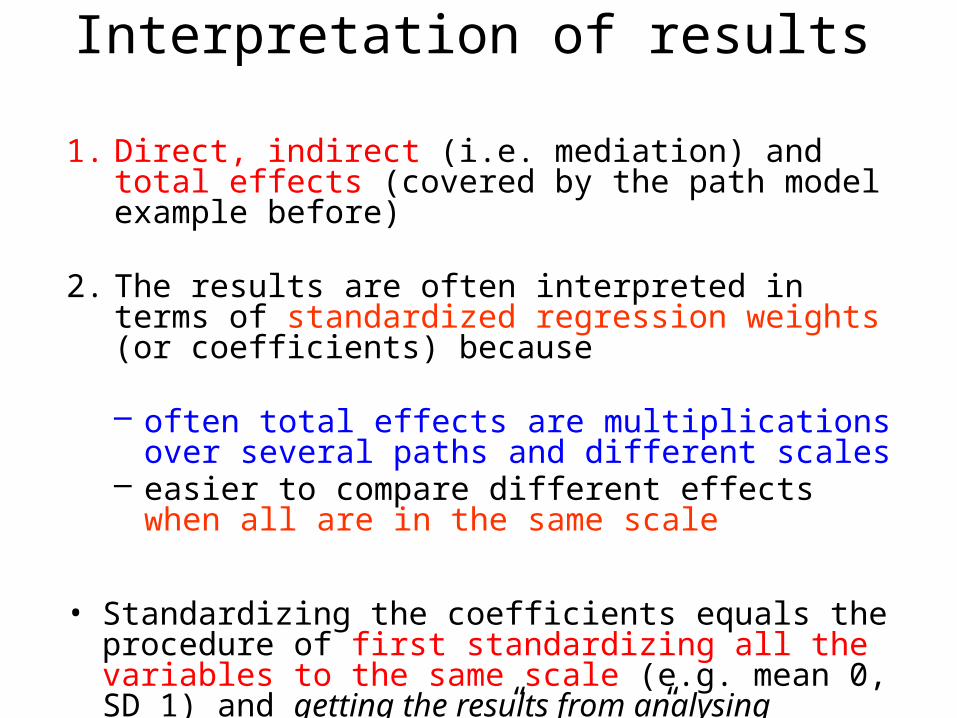
Interpretation of results

1. Direct, indirect (i.e. mediation) and total effects (covered by the path model example before)

2. The results are often interpreted in terms of standardized regression weights (or coefficients) because

– often total effects are multiplications over several paths and different scales

– easier to compare different effects when all are in the same scale

• Standardizing the coefficients equals the procedure of first standardizing all the variables to the same scale (e.g. mean 0, SD 1) and getting the results from analysing standardized variables ”SCALING”..

Standardized regression weights

• For continuos covariates:

bSTDYX=b*SD(X)/SD(Y)

= the change in Y in Y SD units for a standard deviation change in X

• For binary covariates:bSTDY=b/SD(Y)

= the change in Y in Y SD units when X changes from 0 to 1

Standardized regression weightsExample

Height Y: Mean(Y)=164.7, SD(Y)=6.3Weight X: Mean(X)=64.9, SD(X)=11.9

height=a + b*weight +e

b=0.17: – one kg increase in weight increases height by 0.17cm

bSTDYX=0.17*11.9/6.3=0.32 – a SD change in X (11.9 kg) increases Y by 0.32 Y SD

units, i.e. 0.32*6.3cm=2.02cm

Model estimation

Inference is based on the multivariate likelihood function; the maximum likelihood approach

Software: in Stata, MPlus, LISREL, Amos, SAS and R (but for less general models).

Potential biasesOur interpretation of results obtained from a multivariatemodel depends on the appropriateness of the assumedstructure and the quality of the available data.

We cannot interpret the estimated effects as causal withoutconsidering whether:

• conceptual model is correct; need to ask questions like

Are there any unaccounted confounding factors? Are the measures of effect specified on the correct scale?

• the quality of the data is satisfactory: Are the data affected by:

1) measurement error?2) systematic missingness?

Rubin’s classification (1987):

MCAR: missing completely at random;MAR: missing at random;MNAR: missing not at random

If missingness is assumed to be MAR,one approach isMultiple Imputation (MI). Its aim is to integrate the‘substantive’ model likelihood over the missing values.

In practice MI consists of an imputation step and ananalytical step which are repeated m times (for stability andassessment of precision).

Missing data bias

• allows the joint estimation of complex relationships

• assumptions underlying these relationships -althoughmostly untestable- are all explicit

• allows dealing with measurement error directly (alsocan deal with misclassification within the sameframework)

• allows dealing with missing values directly (assumption of MAR)

• assuming model is correct, gives estimates of directand indirect effects

Disease mechanisms.... With reservations

Advantages of a multivariate approach -

• heavily structured

• estimated direct and indirect effects may be grossly biased (and difficult)

• other approaches (e.g. marginal structural models -Hernan et al, Epidemiology, 2004) make fewerparametric assumptions (especially regardingunmeasured confounders) and therefore are morerobust (but could be less efficient if the equivalent SEMwere correct)

Disadvantages of a multivariate approach

These analytic strategies open new ways of understanding better disease mechanisms

Need for a very careful interplay of:

1) subject-knowledge2) data gathering across different sources – time periods3) model specification and fitting to deal with:

Structure: Quality:temporal associations measurement error‘causal’ association missing values

proxy variables

4) sensitivity analyses on the less developed sections5) comparisons across different studies – REPLICATION!

Summary, message...

Smoking and Blood Pressure

• Several studies show lower BP in smokers (Leone 2011. Cardiol Res Pract 2011: 264894)

• BUT, in the long run, smoking increases arterial stiffness thus partly contributing to rising BP (Leone 2011. Cardiol Res Pract 2011: 264894)

CHRNA - GENE CLUSTER ENCODES NICOTINIC ACETYLCHOLINE RECEPTOR SUBUNITS

TTC12-ANKK1-DRD2 – DOPAMIN METABOLISM, LINKED WITH NICOTININ USE, DEPENDENCIES

Pathways leading to smoking behaviour – reference with blood pressure

To catch-up: many types of changes in genome - single-nucleotide polymorphisms (SNPs), tandem repeats, copy number of variation (CNV), inversions, deletions

DNA molecule 1 differs from DNA molecule 2 at a single base-pair location (a C/T polymorphism)Sugar-phosphate backbone; rangs are nucleotide base pairs (C combines with G, A with T)

A = adenineT = thymineC = cytosineG = guanine

ATG CTG..“sentences”=genes

Gene -> proteins

after further adjustment for multiple testing, power issue

after adjustment for sex, BMI,PCs

Smoking at 14

Maternal smoking during

pregnancy

TTC12-rs10502172[G] CHRNA3-rs1051730[A]

Family SES at 14

SEX (F vs M)

Prenatal family SES

Maternal marital status at birth

High Novelty seeking

SES at 31

SBP at 31

Shared genetics between smoking and SBP

Smoking at 31

Conclusions and Future aspects

• Some evidence for an association between variants in the CHRNA5-CHRNA3-CHRNB4 and SBP (in smokers)

• Replication needed – CARTA – consortium; Mendelian randomization approach

• Lifecourse analyses

Maternal Smoking at the 2nd Month of

Pregnancy

Maternal Pre-

Pregnancy BMI

Parity

Family SES at Birth

BMI at Birth

Gestational Age

GenderAlcohol

Use at Age 31 Years

DISTAL PHENOTYPE

-BMI

SES at Age 31 Years

BMI at Age 14 Years

GENE- FTO

Physical Activity at Age

31 Years

Alcohol Use at Age 14 Years

Smoking at Age 14 Years

Maternal Age

Smoking at Age 31

Years

Physical Activity at

Age 14 Years

Family SES at Age 14

Years

Diet at Age 31 Years

Maternal Blood Pressure During

Pregnancy

Prenatal Birth Childhood Adolescence Adulthood

1. ”Spider diagram” challenge -

life-course analyses of FTO using path analysis (SEM)

Direct, indirect and total effects of FTO on adult BMI (standardized beta values)• Direct effect: 0.04

• Indirect effects of the FTO variant to adult BMI:– FTO-mat.BMI-BMI31: 0.03*0.095=0.003– FTO-mat.BMI-BBMI-BMI14-BMI31: 0.03*0.155*0.08*0.529=0.002– FTO-BBMI-BMI14-BMI31: 0.018*0.08*0.529=0.001– FTO-BMI14-BMI31: 0.026*0.529=0.014– Total indirect: 0.003+0.002+0.001+0.014=0.020

• Total effect: 0.02+0.04=0.06

0.095

0.5290.08

0.026

0.03

0.175

0.018

0.155

0.04

0.25

0.16

Direct, Indirect and Total Effects of FTO-rs9939609 on Body Mass Index (BMI) During the Life Course in the Northern Finland Birth

Cohort 1966 (adjusting for all other factors). Note – SES, physical activity, maternal parity had large effects

Abbreviations: BMI, body mass index; CI, confidence interval., BMI log transformed

Effect of FTO-rs99309609 P value Change in the mean level of

BMI (g/m2), per A-allele change

95% CI

Total 5.0x10-5 371 185, 570

Total indirect (via …) 0.02 121 19.6, 227

Direct 0.001 239 89.6, 396

Acknowledgements… OULUM JarvelinA TaanilaA PoutaA-L Harti-KainenM LeinonenJ VeijolaA RuokonenM IsohanniM SavolainenK-H Hertzig

HelsinkiL PalotieT PaunioJ EkelundE NymanH Mannila

KuopioJ Pekkanen+team

UppsalaA Rodriquez

CopenhagenJ OlsenT Sörensen

LONDON/UKP ElliottL CoinJ ChambersM LevinA BlakemoreJ KoonerU SovioP O’ReillyD PillasM McCarthyD CanoyG Davey SmithT FraylingG Schumann

LilleP Froquel S CauchiN Boutia-Naji

AthensC Bakoula +team

BergenE Heiervang

TampereSuvi Virtanen

LAF NelsonS SmalleyJ McCoughC SabattiS Service

BonnDLichterman

Dallas

AustraliaMcGrathL PalmerL CoinE Hypponen

BostonJ HirschhornM DalyH Lyon

NEW ZEALANDW CaulfieldW SchierdingJ O’Sullivan P Davies et al..