NÚÑEZ AND ANDRÉS TRUJILLO-BARRERA Impact of … · Impact of U.S. Biofuel Policy in the Presence of Drastic Climate Conditions . ... the markets to adjust to new ... out of methyl

NÚMERO 585

HÉCTOR M. NÚÑEZ AND ANDRÉS TRUJILLO-BARRERA

Impact of U.S. Biofuel Policy in the Presence of Drastic Climate Conditions

www.cide.edu NOVIEMBRE 2014

Importante Los Documentos de Trabajo del CIDE son una herramienta para fomentar la discusión entre las comunidades académicas. A partir de la difusión, en este formato, de los avances de investigación se busca que los autores puedan recibir comentarios y retroalimentación de sus pares nacionales e internacionales en un estado aún temprano de la investigación. De acuerdo con esta práctica internacional congruente con el trabajo académico contemporáneo, muchos de estos documentos buscan convertirse posteriormente en una publicación formal, como libro, capítulo de libro o artículo en revista especializada.

http://www.cide.ed/

D.R. © 2014, Centro de Investigación y Docencia Económicas A.C. Carretera México Toluca 3655, Col. Lomas de Santa Fe, 01210, Álvaro Obregón, México DF, México. www.cide.edu www.LibreriaCide.com Dirección de Publicaciones [email protected] Tel. 5081 4003

http://www.libreriacide.com/

Abstract We analyze the impact of total and partial waivers of the U.S. Renewable Fuel Standard (RFS) under uncertain changes in climate conditions that affects crop yields distributions. The main model results show that reducing RFS would make world agricultural consumers better off, and increase U.S. corn share in the world market, while slightly decrease agricultural commodity prices, but the higher the RFS reduction the higher the uncertainty on the price changes. On the other hand, price changes would make ethanol and agricultural producers face losses as well as increase gasoline consumption and, therefore, bringing larger environmental damages. Overall RFS reduction generates negative changes in total economic surplus, specifically, RFS reductions up to 40 percent generate significant changes in the socio-economic variables, however any reductions beyond 40 percent do not appear to bring further changes, although welfare results appear more uncertain under an increased reduction. JEL classification: Q10, Q48, Q54 Keywords: Biofuel Policy, Climate Uncertainty, Crop Commodity Markets

Resumen

En este trabajo analizamos el impacto de exensiones total y parciales al estándar de combustible renovable (RFS) de EE.UU en un contexto de incertidumbre ante el cambio climático que afecta la productividad agrícola. Los resultados principales del modelo muestran que una reducción del RFS prodría generar una mejoría para los agricultores del mundo, pero a medida que se reduce la incertidumbre en el cambio de los precios aumenta. Por otro lado, el cambio en los precios podría hacer que los productores de etanol y agricultores enfrenten pérdidas de bienestar, así como se de un incremento en el consumo de gasolina y, por lo tanto, conlleve a daños ambientales mayores. En conjunto, la reducción del RFS genera cambios negativos en el excedente total de la economía, en específico, reducciones hasta del 40 por ciento pueden generar cambios significativos en las variables económicas, no obstante, reducciones mayores a este nivel no parecen conllevar a más cambios, pero si a mayor incertidumbre sobre los cambios en el bienestar. Clasificación JEL: Q10, Q48, Q54 Palabras Clave: Políticas de Biocombustibles, incertidumbre climática, mercado de materias primas agrícolas

Impact of U.S. Biofuel Policy in the Presence of Uncertain Climate Conditions

Introduction

he increase of the ethanol industry in the U.S. has been the result of a mix of policy and economic factors that have led to the use of about 40 percent of the corn crop as input for ethanol production, and about 10 percent of the car-fuel

content in the U.S. Considerable effort has been made to assess the social, environmental, and economic impacts of the ethanol boom. Yet, less work has analyzed the effects of biofuel policies under uncertain climate conditions, which affect crop yield throughout all the country.

The interest on weather uncertainty and its relationship with biofuel policy became more salient after the drought of 2012 in the U.S., when substantial corn price fluctuations brought back concerns about the role of biofuels on food security and food prices. The U.S. Environmental Protection Agency (EPA) considered a request of a partial or total waiver of the Renewable Fuel Standard (RFS) for 2012 and 2013, but declined it claiming that biofuel policy would not have a significant effect on market outcomes in the short term. In this study we analyze the impact of U.S. biofuel policies when crop yields vary due to changes in climate conditions. We project market conditions to 2022 to allow the markets to adjust to new equilibria, and to match the deadlines of the RFS goals.

Given that the U.S. is the world's largest producer and exporter of grains and oilseeds (USDA-ERS, 2012), biofuel policies leading the use of domestic corn for ethanol production have significant implications not only for U.S. crop and livestock production, but also for global trade and international markets. The purpose of this study is to evaluate the effects of the current U.S. biofuel policy, analyzing scenarios of total or partial waiver of RFS in conjunction with uncertainty on climate conditions via Monte Carlo simulations for each of the main crops’ yields in all the agricultural districts of the U.S.

Our analysis encompasses the agricultural and fuel sectors of the U.S. and Brazil, and the agricultural sector of Argentina in a static simultaneous framework, which allows us to examine the changes in market equilibrium conditions. In addition to bilateral trade between these countries, we include food/feed and biofuel demand of China and the rest of the world (ROW). We analyze effects on price, land use, main crop/commodity and ethanol markets, and economic surplus of producers and consumers. The main goal is to provide a comprehensive view of the effect of biofuel policies in an environment of climate change uncertainty.1 The model is calibrated and validated using 2007 as base year, then we project market conditions to 2022 and introduce uncertainty due to weather conditions by considering alternative parametric distributions specifications for crop yields of the main crops in the U.S

1 This paper focuses only on ethanol market and does not incorporate biodiesel production to keep the analysis tractable.

T

DIVISIÓN DE ECONOMIA

1

Hector M. Nuñez and Andrés Trujillo-Barrera

We use the uniform and beta distributions following related literature (Claassen and Just, 2011; Norwood et al., 2004), estimating parameters from historical yields for each of the agricultural districts in the U.S. We replicate this model 1,000 times drawing yields with replacement to find the distribution of the variables analyzed in the agricultural and fuel markets scenario in 2022. Since RFS level is not a random decision, we considers several scenarios of partial and total waiver, therefore we report results under different mandate levels.

Results show that reducing ethanol mandates would make world agricultural consumers better off, and increase U.S. corn share in the world market, while slightly decreasing agricultural commodity prices. However, ethanol and agricultural producers would face losses and environmental damage would increase. Overall RFS reduction generates negative changes in total economic surplus of the related sectors in the model, but most of the changes occur up to 40 percent RFS reduction. Larger reductions (above 40 percent) do not appear to generate further changes in the markets, however, a slight increase in uncertainty of welfare results is observed with higher reductions.

Background and Previous Work

Ethanol production in the U.S. has been driven by biofuel policy over the last decade, most notably by the regulations on fuels composition under the RFS, which was introduced by the Energy Policy Act of 2005 and later amended by the Energy Independence and Security Act of 2007. RFS established a mandate that requires transportation fuels to contain a minimum amount of fuel from renewable sources each year with a goal of 136.27 billion liters of biofuel production by 2022, with a maximum of 56.78 billion liters of conventional or first-generation ethanol by 2015. Current RFS regulations state that all gasoline-powered vehicles may use a fuel blend with up to 15 percent of ethanol content (E15 or E10), while flex fuel vehicles may use a fuel blend up to 85 percent ethanol content (E85), however, E85 consumption is still very small. As a result, to date, almost 10 percent of car fuel consumption in the U.S. comes from corn-based ethanol (Renewable Fuels Association, 2013). In turn, about 40 percent of the corn crop is devoted to ethanol production.2 Besides biofuel policy, economic considerations also justify blending ethanol into gasoline. Babcock (2011) and Babcock and Zhou (2013) argue that high gasoline prices and the phase out of methyl tertiary butyl ether (MTBE) as oxygenate additive of gasoline in the mid-2000s, also played an important role in the surge of the ethanol

2 Although the RFS is the central instrument of U.S. biofuel policy, other policy mechanisms including subsidies to ethanol blenders such as. the volumetric ethanol excise tax credit,, and tariffs to ethanol imports, played a significant role during the development of the ethanol industry but those instruments expired by 2012 (U.S. Farm Bill 2008; Energy Improvement and Extension Act 2008; U.S. International Trade Comission 2011; Energy Policy Act 2005).

CIDE

2


industry. As long as ethanol prices are competitive in relation to gasoline, ethanol production is economically viable, even in the absence of the mandate and subsidies.

The economic, social, and environmental effects of the biofuel policy and ethanol production have received substantial attention in the literature. Although the quantification of those effects is confounded by complex and interlinked factors, the increase in corn use for ethanol production is regarded as a major driver of crop price fluctuations (Baffes et al., 2011; Gilbert and Morgan, 2010; Hochman et al., 2011; Wright, 2011). Also leading to land and water use changes in the U.S., and in other ethanol and grain producer countries like Brazil and Argentina, where different crops compete for land (Fabiosa et al., 2010; Timilsina et al., 2012; Zilberman et al., 2012). As a result, U.S. biofuel policy becomes a contributing factor in world’s agricultural markets.

Until recently, weather events associated with climate change did not seem to play a crucial role for agricultural commodity markets during the ethanol boom. However, as identified by Babcock and Zhou (2013), the 2012 drought in U.S. Corn Belt brought back attention to the purpose of policies that promote the corn ethanol industry. The U.S. Environmental Protection Agency (EPA), the agency in charge of the administration of RFS, has considered several times to issue a partial or full waiver of the mandate. For instance, after the drought of 2012, a formal request from Governors from several States was declined by Environmental Protection Agency (EPA) on the grounds that waiving the mandate would have little if any impact on ethanol demand or energy prices over that time period, and no evidence was found of the federal RFS causing severe ‘economic harm’, although the agency recognizes significant hardships in many sectors of the economy created by the drought (EPA, 2012). Later, by the end of 2013 EPA announced a preliminary RFS rulemaking for 2014, with a proposal to decrease the ethanol mandate from 54.5 (14.4) to 49.2 (13) billion liters (gallons), acknowledging constraints in the market’s ability to consume renewable fuels in coming years at the volumes specified by the Clean Air Act. The proposal has been the subject of heated debate, and the final decision has been delayed longer than the initial deadlines. Roberts and Tran (2013) argue that given that ethanol now accounts for more than 40 percent of the U.S. annual corn harvest together with the current increasing trend of uncertain weather events, it is likely that similar requests to EPA to waive the U.S. ethanol mandate will happen again in the future.

The extent of the influence of a partial or total waiver of the mandate depends on several circumstances, as explained by Babcock (2012), Tyner (2010) ,Tyner, Taheripour, & Hurt (2012), and Babcock and Zhou (2013). First, is expected that a waiver would not have a strong effect on the short term, since sunk costs, and ongoing investment and production decisions are unlikely to be changed by the elimination or decrease of the mandate, therefore the main effects of the waiver decision should be evaluated at a longer term. Further, the influence of the mandate depends on the extent of the competitiveness of ethanol as a fuel substitute. Ethanol is economically viable, as octane enhancer, and also as a blend, as long as its equivalent energy content


3


is cheaper than gasoline.3 Therefore, the mandate incentives become relevant under a scenario of low to moderate energy prices, strong export demand, low ethanol stocks, and high corn prices, where crop yield uncertainty may affect the last three.

Several studies have examined the potential effect of a RFS waiver under uncertain crop conditions. Findings from the literature show strong variations depending on the modeling approach, underlying assumptions, and the degree and length of the mandate suspension. Condon, Klemick, and Wolverton (2013) reviewed the current literature on the impact of ethanol policy on corn prices, finding that long-run analyses released between 2008 and 2012 show an average corn price increase between 2 and 3 percent for each extra billion gallons of corn-ethanol in the market.

Tokgoz et al. (2008) developed a scenario of short crop with ethanol mandate for 2012-2013. Their results suggest that a decline on the production of corn and soybean would decrease exports and stock levels. As a result, corn exports from South America increase, and the amount of corn fed livestock decreases. However, the effects of the supply shock transmitted to other sectors are considered only temporary. In addition, allowing free trade of ethanol is advisable, since it may attenuate the negative impact of short crops.

Some of the recent literature has considered RFS suspension with a focus on the 2012 drought. Carter, Rausser, and Smith (2012) quantified the effect of ethanol production in corn prices using a Structural Vector Autoregression model (SVAR), finding corn prices about 40 percent lower in 2012 without the RFS mandate, concluding that the impact of the U.S. energy policy on global corn prices is considerable, affecting particularly the world’s poor.

Meanwhile, Roberts and Tran (2013) use a competitive storage model focused on the U.S. domestic market to analyze a suspension of the RFS mandate in 2012 on prices and storage of corn, finding that although a price reduction would only be modest, the reduction in price volatility would be substantial. Furthermore they found consumer welfare gains associated to lower corn prices in the U.S.

Most of the current discussion of the effects of the mandate has centered on price effects and also tradeoffs between corn producers and corn users such as ethanol and livestock producers. In this paper we complement and extend the analysis of the biofuel policies under the weather uncertainty scenarios by looking in the long-run at effects such as trade, land use, and overall welfare. Further, the U.S. biofuel programs also impact and interact with the rest of the world (Hertel et al., 2010; Searchinger et al., 2008), in our analysis we incorporate other big players of the ethanol and corn markets such as Brazil, Argentina, and China.

3 Ethanol contains about 70% of the energy content of gasoline.

CIDE

4


The model

As a policy analysis tool we use a price endogenous mathematical programming model similar to that in Nunez et. al. (2013), but including a module to model the climate uncertainty. A detailed mathematical version of the model is presented in the appendix.

The model is a multi-region, multi-market, multi-product, spatial equilibrium model that includes the agricultural and fuel sectors of the U.S. and Brazil, and the agricultural sector of Argentina. In addition to bilateral trade between these countries the food/feed and biofuel demand of China and the rest of the world (ROW) are also part of the model. Consumers’ surplus is derived from consumption of agricultural commodities and transportation fuels by light-duty vehicles that generate vehicle-kilometers-traveled, which generates implicitly the demand for ethanol and gasoline restricted to the technical and policy restrictions.

The model assumes an upward sloping supply function for gasoline in the U.S., ROW, and China components while in the case of Brazil a perfectly elastic supply function is assumed reflecting the constant pricing policy for pure gasoline at the refinery level. The demand and supply functions are assumed to be linear and separable, except the crop supply, modeled in detail at regional level by using Leontief production functions for the U.S., Brazil, and Argentina.

Cost functions include all taxes, subsidies, and marketing margins for fuel demand in Brazil and the U.S. Also, the cost of producing ethanol, co-product credits, the cost of converting new lands from pasture uses to cropland in Brazil and from marginal lands to cropland in the U.S. In addition, the cost of producing energy crops, and the cost of collecting crop residue for conversion to biomass. Further, the cost of processing soybean to soymeal and soy oil, sugar beets and sugarcane to sugar, and the cost of raising beef-cattle in Brazil. Finally, we include internal and external costs of transportation.

The maximization problem is subject to resource limitations, mainly land, policy restrictions, material balance, and technical constraints. Ethanol supply depends on the ethanol productivity of the feedstock (i.e. corn and cellulosic in the U.S. and sugarcane in Brazil) and the feedstock yield, which in turn depends on the region where crop is planted. The model includes a constraint for U.S. biofuel mandates, as implied by the revised RFS (excluding the Biomass-based diesel); feedstock for cellulosic biofuel in the U.S. is assumed to come from corn stover, wheat straw, and from two perennial grasses, namely miscanthus and switchgrass.

The agricultural supply side of the model is regionally disaggregated at Crop Reporting District level for the U.S. component, at mesoregion level for Brazil, and at province level for Argentina. In the three regionally disaggregated components, the model includes beef cattle production in Brazil as well as production of corn, sugarcane and thirteen other main temporal crops including soybeans and wheat, allowing commonly practiced intra-year and inter-year crop rotation activities in the three


5


countries. The comparative advantage between crop and livestock activities in each region is modeled explicitly based on national and world prices, costs of production, processing costs, costs of transportation, and regional yields.

Commodity supply is the sum of regional production, which depend on the row crop yield and the amounts of land allocated to that crop determined endogenously. The model includes the possibility of crop-land expansion over pasture land in Brazil. Total land use in each region is restricted to the sum of the total cropland available in the base year, the total pasture land available in Brazil, and the total marginal land available in the U.S.

To incorporate uncertainty due to weather conditions and its effect on the U.S. agricultural output, we model crop yields distributions. We use uniform and beta distributions. The beta distribution is often used in the crop insurance literature for its flexibility, and relatively satisfactory in-sample and out-of-sample performance (Woodard and Sherrick, 2011), and has also been used to model crop yields distributions in the ethanol policy literature (Babcock and Zhou, 2013). Data to estimate the parameters of the distributions correspond to yields reported by the U.S. Department of Agricultural (USDA-NASS, 2012) at Agricultural District level. Parameters of the beta are obtained following a procedure described in Woodard and Sherrick (2011). First, to account for technological change, we estimate the trend via Huber M –estimator, then the detrended data is used to find the parameters of the distribution (Woodard and Sherrick, 2011; Yu and Babcock, 2010).

Next, we replicate the model 1,000 times drawing with replacement yields from the beta distribution using the estimated parameters. We repeat the same procedure with a uniform distribution taking as the two boundaries the lowest and highest yield in the period 2007-2013 of each crop in each district. Because of the high number of simulations using all crops, we restrict the replications only to the main crops in the U.S. Replication results allow us to find the distribution of the variables analyzed in the agricultural and fuel markets scenarios described in section 5.

Data Description

The model is calibrated and validated using 2007 as the base year. Data inputs include the base year domestic and global commodity prices and quantities demanded, historical crop mixes (areas planted to individual crops), crop yields, costs of production and processing, and cost of transportation.

The U.S. crops sector includes sugarcane, alfalfa (semi-perennial crops) and twelve major row annual crops/commodities: corn, soybeans, wheat, sugar beets, barley, sorghum, oats, peanuts, cotton, rice and corn silage. The costs of production for row crops in the U.S. include variable operating costs (seed and treatment, fertilizer, hauling and trucking, drying and storage costs, interest on operating cost), fixed operating

CIDE

6


costs (limestone, chemical costs, fuel and oil, tractor and machinery, crop insurance, marketing and miscellaneous, stock quota lease, irrigation), capital and overhead costs (machinery and building depreciation cost, interest on investment, overhead), and hired labor costs, while the model determines the land price endogenously.

Similarly, for Brazil, the model considers sugarcane and eight major annual crops: soybeans, corn, wheat, sorghum, cassava, dry-beans, cotton and rice, and beef-cattle production. Finally, for Argentina, the model includes only corn, soybean and wheat. Additionally the model considers processing products from soybean, sugarcane, and sugar beets.

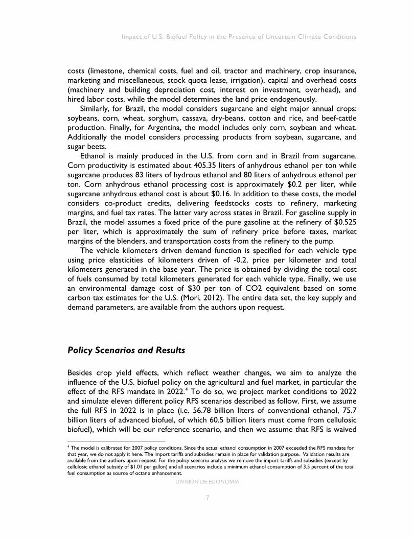
Ethanol is mainly produced in the U.S. from corn and in Brazil from sugarcane. Corn productivity is estimated about 405.35 liters of anhydrous ethanol per ton while sugarcane produces 83 liters of hydrous ethanol and 80 liters of anhydrous ethanol per ton. Corn anhydrous ethanol processing cost is approximately $0.2 per liter, while sugarcane anhydrous ethanol cost is about $0.16. In addition to these costs, the model considers co-product credits, delivering feedstocks costs to refinery, marketing margins, and fuel tax rates. The latter vary across states in Brazil. For gasoline supply in Brazil, the model assumes a fixed price of the pure gasoline at the refinery of $0.525 per liter, which is approximately the sum of refinery price before taxes, market margins of the blenders, and transportation costs from the refinery to the pump.

The vehicle kilometers driven demand function is specified for each vehicle type using price elasticities of kilometers driven of -0.2, price per kilometer and total kilometers generated in the base year. The price is obtained by dividing the total cost of fuels consumed by total kilometers generated for each vehicle type. Finally, we use an environmental damage cost of $30 per ton of CO2 equivalent based on some carbon tax estimates for the U.S. (Mori, 2012). The entire data set, the key supply and demand parameters, are available from the authors upon request.

Policy Scenarios and Results

Besides crop yield effects, which reflect weather changes, we aim to analyze the influence of the U.S. biofuel policy on the agricultural and fuel market, in particular the effect of the RFS mandate in 2022.4 To do so, we project market conditions to 2022 and simulate eleven different policy RFS scenarios described as follow. First, we assume the full RFS in 2022 is in place (i.e. 56.78 billion liters of conventional ethanol, 75.7 billion liters of advanced biofuel, of which 60.5 billion liters must come from cellulosic biofuel), which will be our reference scenario, and then we assume that RFS is waived

4 The model is calibrated for 2007 policy conditions. Since the actual ethanol consumption in 2007 exceeded the RFS mandate for that year, we do not apply it here. The import tariffs and subsidies remain in place for validation purpose. Validation results are available from the authors upon request. For the policy scenario analysis we remove the import tariffs and subsidies (except by cellulosic ethanol subsidy of $1.01 per gallon) and all scenarios include a minimum ethanol consumption of 3.5 percent of the total fuel consumption as source of octane enhancement.


7


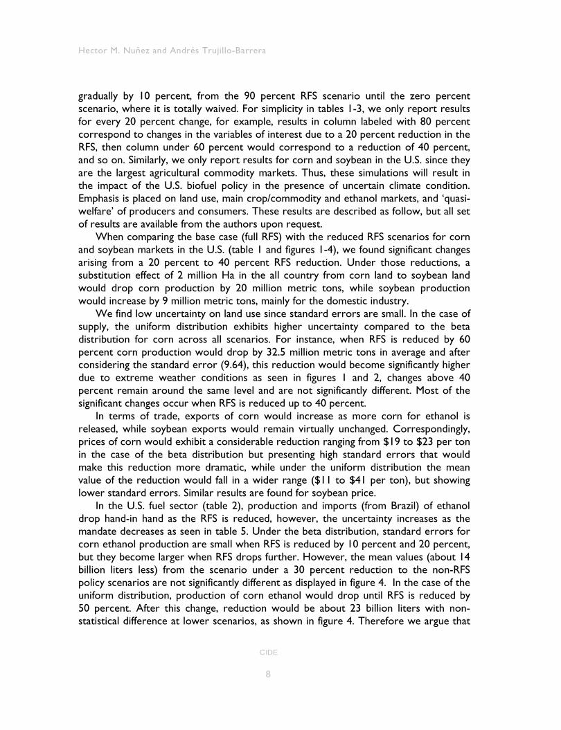
gradually by 10 percent, from the 90 percent RFS scenario until the zero percent scenario, where it is totally waived. For simplicity in tables 1-3, we only report results for every 20 percent change, for example, results in column labeled with 80 percent correspond to changes in the variables of interest due to a 20 percent reduction in the RFS, then column under 60 percent would correspond to a reduction of 40 percent, and so on. Similarly, we only report results for corn and soybean in the U.S. since they are the largest agricultural commodity markets. Thus, these simulations will result in the impact of the U.S. biofuel policy in the presence of uncertain climate condition. Emphasis is placed on land use, main crop/commodity and ethanol markets, and ‘quasi-welfare’ of producers and consumers. These results are described as follow, but all set of results are available from the authors upon request.

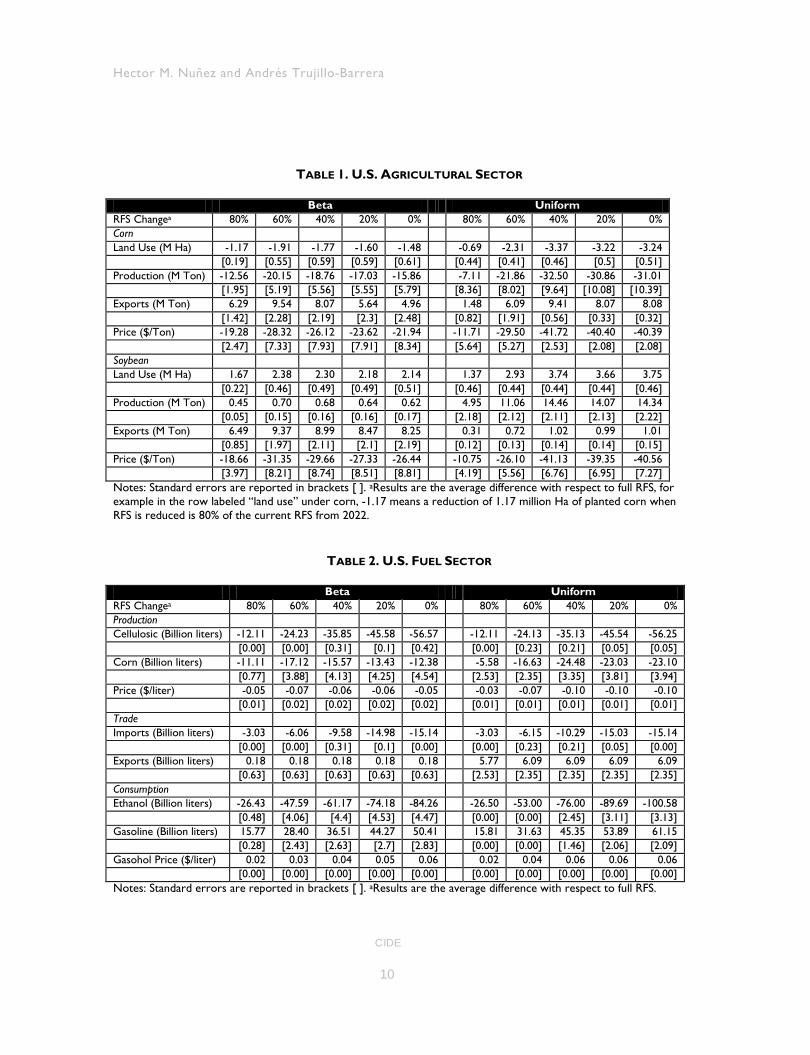
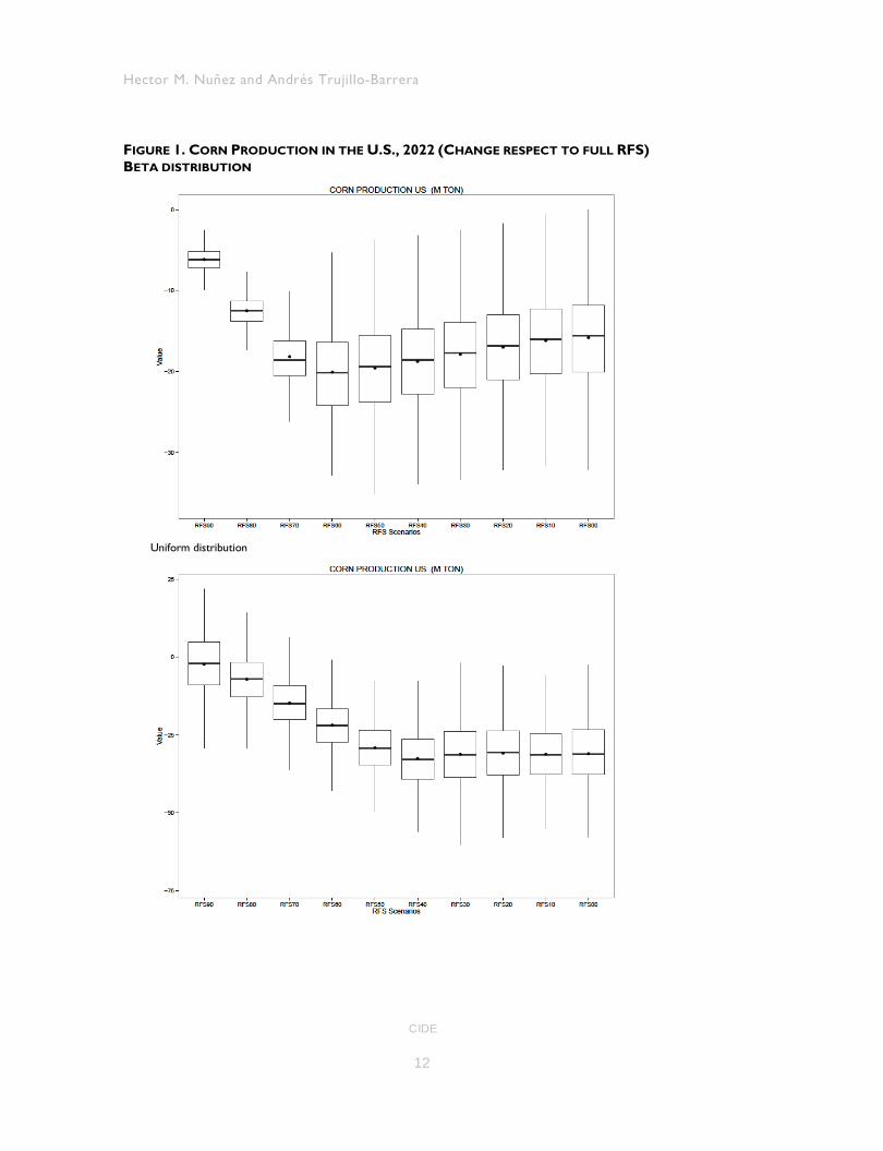
When comparing the base case (full RFS) with the reduced RFS scenarios for corn and soybean markets in the U.S. (table 1 and figures 1-4), we found significant changes arising from a 20 percent to 40 percent RFS reduction. Under those reductions, a substitution effect of 2 million Ha in the all country from corn land to soybean land would drop corn production by 20 million metric tons, while soybean production would increase by 9 million metric tons, mainly for the domestic industry.

We find low uncertainty on land use since standard errors are small. In the case of supply, the uniform distribution exhibits higher uncertainty compared to the beta distribution for corn across all scenarios. For instance, when RFS is reduced by 60 percent corn production would drop by 32.5 million metric tons in average and after considering the standard error (9.64), this reduction would become significantly higher due to extreme weather conditions as seen in figures 1 and 2, changes above 40 percent remain around the same level and are not significantly different. Most of the significant changes occur when RFS is reduced up to 40 percent.

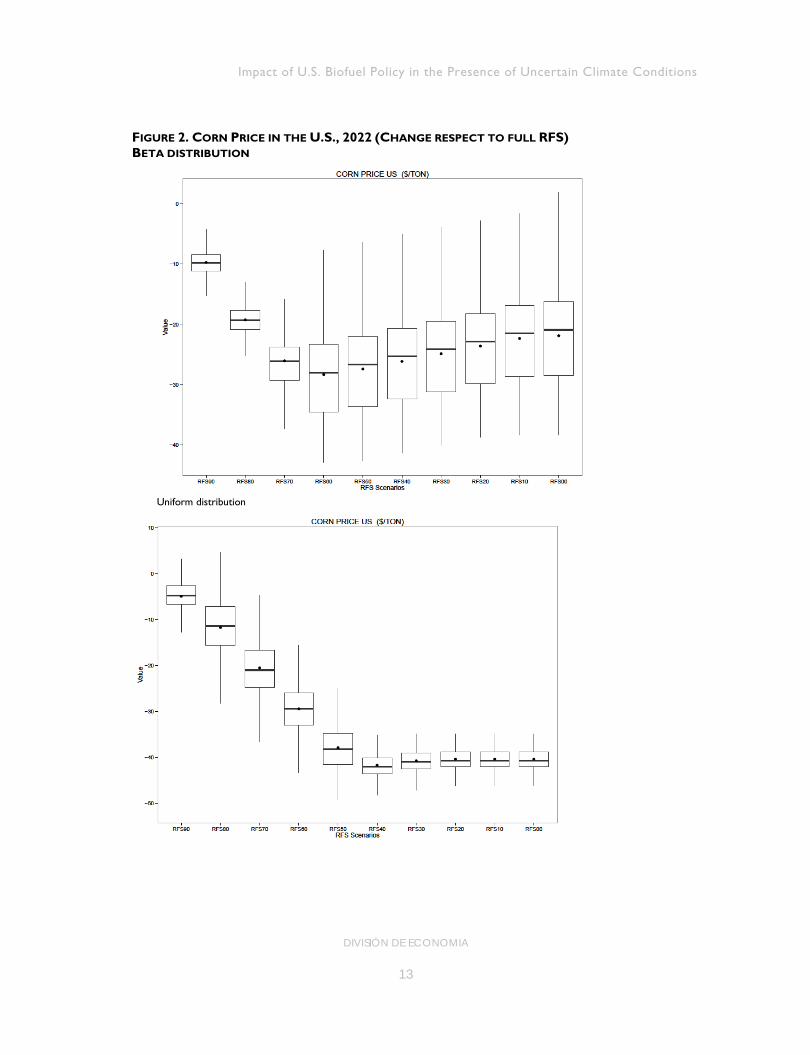
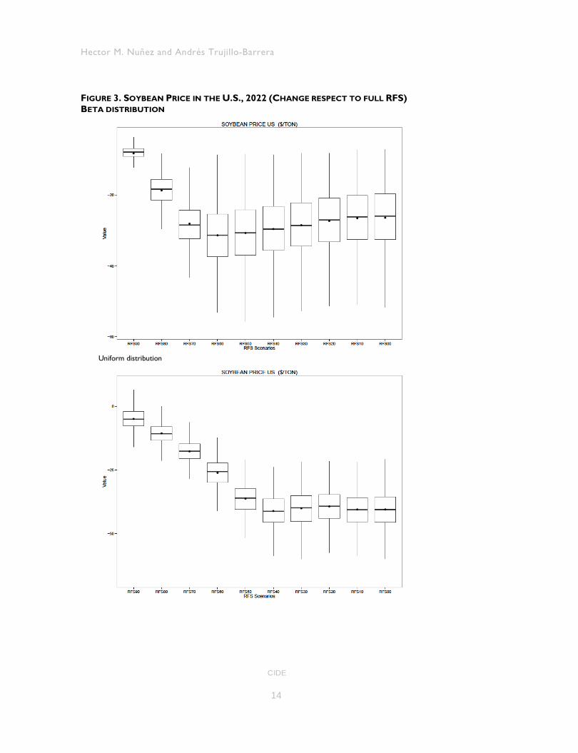
In terms of trade, exports of corn would increase as more corn for ethanol is released, while soybean exports would remain virtually unchanged. Correspondingly, prices of corn would exhibit a considerable reduction ranging from $19 to $23 per ton in the case of the beta distribution but presenting high standard errors that would make this reduction more dramatic, while under the uniform distribution the mean value of the reduction would fall in a wider range ($11 to $41 per ton), but showing lower standard errors. Similar results are found for soybean price.

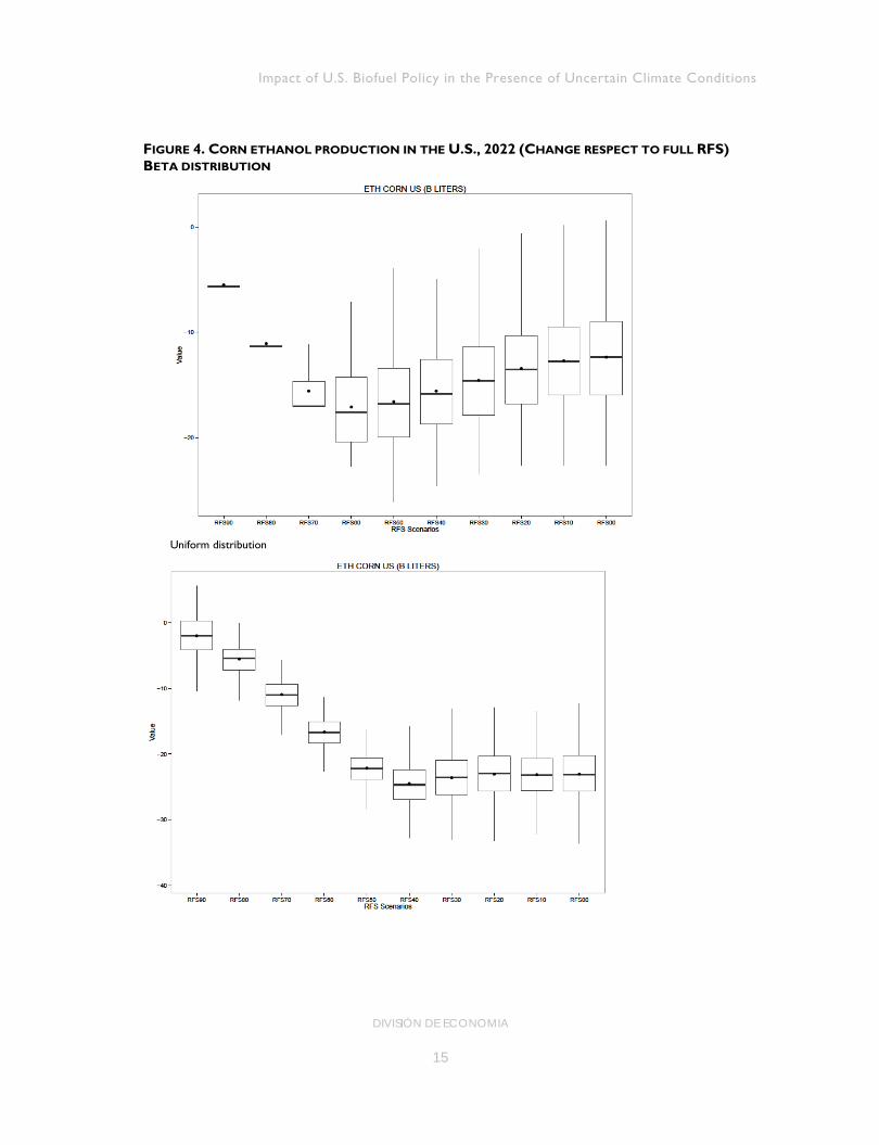
In the U.S. fuel sector (table 2), production and imports (from Brazil) of ethanol drop hand-in hand as the RFS is reduced, however, the uncertainty increases as the mandate decreases as seen in table 5. Under the beta distribution, standard errors for corn ethanol production are small when RFS is reduced by 10 percent and 20 percent, but they become larger when RFS drops further. However, the mean values (about 14 billion liters less) from the scenario under a 30 percent reduction to the non-RFS policy scenarios are not significantly different as displayed in figure 4. In the case of the uniform distribution, production of corn ethanol would drop until RFS is reduced by 50 percent. After this change, reduction would be about 23 billion liters with non-statistical difference at lower scenarios, as shown in figure 4. Therefore we argue that

CIDE

8


climate uncertainty would not make a large difference in the production of conventional ethanol in the U.S. if RFS were lower than the current standard.

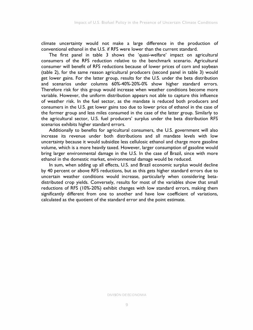
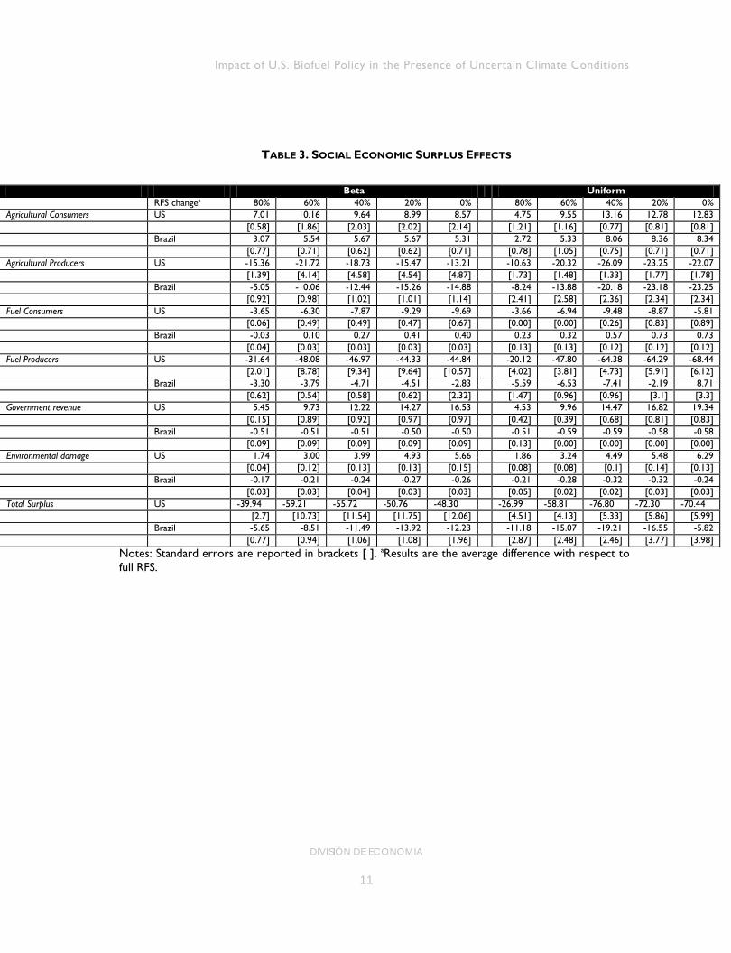
The first panel in table 3 shows the ‘quasi-welfare’ impact on agricultural consumers of the RFS reduction relative to the benchmark scenario. Agricultural consumer will benefit of RFS reductions because of lower prices of corn and soybean (table 2), for the same reason agricultural producers (second panel in table 3) would get lower gains. For the latter group, results for the U.S. under the beta distribution and scenarios under columns 60%-40%-20%-0% show higher standard errors. Therefore risk for this group would increase when weather conditions become more variable. However, the uniform distribution appears not able to capture this influence of weather risk. In the fuel sector, as the mandate is reduced both producers and consumers in the U.S. get lower gains too due to lower price of ethanol in the case of the former group and less miles consumed in the case of the latter group. Similarly to the agricultural sector, U.S. fuel producers’ surplus under the beta distribution RFS scenarios exhibits higher standard errors.

Additionally to benefits for agricultural consumers, the U.S. government will also increase its revenue under both distributions and all mandate levels with low uncertainty because it would subsidize less cellulosic ethanol and charge more gasoline volume, which is a more heavily taxed. However, larger consumption of gasoline would bring larger environmental damage in the U.S. In the case of Brazil, since with more ethanol in the domestic market, environmental damage would be reduced.

In sum, when adding up all effects, U.S. and Brazil economic surplus would decline by 40 percent or above RFS reductions, but as this gets higher standard errors due to uncertain weather conditions would increase, particularly when considering beta-distributed crop yields. Conversely, results for most of the variables show that small reductions of RFS (10%-20%) exhibit changes with low standard errors, making them significantly different from one to another and have low coefficient of variations, calculated as the quotient of the standard error and the point estimate.


9


TABLE 1. U.S. AGRICULTURAL SECTOR

Beta Uniform RFS Changea 80% 60% 40% 20% 0% 80% 60% 40% 20% 0% Corn Land Use (M Ha) -1.17 -1.91 -1.77 -1.60 -1.48 -0.69 -2.31 -3.37 -3.22 -3.24

[0.19] [0.55] [0.59] [0.59] [0.61] [0.44] [0.41] [0.46] [0.5] [0.51] Production (M Ton) -12.56 -20.15 -18.76 -17.03 -15.86 -7.11 -21.86 -32.50 -30.86 -31.01

[1.95] [5.19] [5.56] [5.55] [5.79] [8.36] [8.02] [9.64] [10.08] [10.39] Exports (M Ton) 6.29 9.54 8.07 5.64 4.96 1.48 6.09 9.41 8.07 8.08

[1.42] [2.28] [2.19] [2.3] [2.48] [0.82] [1.91] [0.56] [0.33] [0.32] Price ($/Ton) -19.28 -28.32 -26.12 -23.62 -21.94 -11.71 -29.50 -41.72 -40.40 -40.39 [2.47] [7.33] [7.93] [7.91] [8.34] [5.64] [5.27] [2.53] [2.08] [2.08] Soybean Land Use (M Ha) 1.67 2.38 2.30 2.18 2.14 1.37 2.93 3.74 3.66 3.75

[0.22] [0.46] [0.49] [0.49] [0.51] [0.46] [0.44] [0.44] [0.44] [0.46] Production (M Ton) 0.45 0.70 0.68 0.64 0.62 4.95 11.06 14.46 14.07 14.34

[0.05] [0.15] [0.16] [0.16] [0.17] [2.18] [2.12] [2.11] [2.13] [2.22] Exports (M Ton) 6.49 9.37 8.99 8.47 8.25 0.31 0.72 1.02 0.99 1.01

[0.85] [1.97] [2.11] [2.1] [2.19] [0.12] [0.13] [0.14] [0.14] [0.15] Price ($/Ton) -18.66 -31.35 -29.66 -27.33 -26.44 -10.75 -26.10 -41.13 -39.35 -40.56 [3.97] [8.21] [8.74] [8.51] [8.81] [4.19] [5.56] [6.76] [6.95] [7.27] Notes: Standard errors are reported in brackets [ ]. aResults are the average difference with respect to full RFS, for example in the row labeled “land use” under corn, -1.17 means a reduction of 1.17 million Ha of planted corn when RFS is reduced is 80% of the current RFS from 2022.

TABLE 2. U.S. FUEL SECTOR

Beta Uniform RFS Changea 80% 60% 40% 20% 0% 80% 60% 40% 20% 0% Production Cellulosic (Billion liters) -12.11 -24.23 -35.85 -45.58 -56.57 -12.11 -24.13 -35.13 -45.54 -56.25

[0.00] [0.00] [0.31] [0.1] [0.42] [0.00] [0.23] [0.21] [0.05] [0.05] Corn (Billion liters) -11.11 -17.12 -15.57 -13.43 -12.38 -5.58 -16.63 -24.48 -23.03 -23.10

[0.77] [3.88] [4.13] [4.25] [4.54] [2.53] [2.35] [3.35] [3.81] [3.94] Price ($/liter) -0.05 -0.07 -0.06 -0.06 -0.05 -0.03 -0.07 -0.10 -0.10 -0.10 [0.01] [0.02] [0.02] [0.02] [0.02] [0.01] [0.01] [0.01] [0.01] [0.01] Trade Imports (Billion liters) -3.03 -6.06 -9.58 -14.98 -15.14 -3.03 -6.15 -10.29 -15.03 -15.14

[0.00] [0.00] [0.31] [0.1] [0.00] [0.00] [0.23] [0.21] [0.05] [0.00] Exports (Billion liters) 0.18 0.18 0.18 0.18 0.18 5.77 6.09 6.09 6.09 6.09 [0.63] [0.63] [0.63] [0.63] [0.63] [2.53] [2.35] [2.35] [2.35] [2.35] Consumption Ethanol (Billion liters) -26.43 -47.59 -61.17 -74.18 -84.26 -26.50 -53.00 -76.00 -89.69 -100.58

[0.48] [4.06] [4.4] [4.53] [4.47] [0.00] [0.00] [2.45] [3.11] [3.13] Gasoline (Billion liters) 15.77 28.40 36.51 44.27 50.41 15.81 31.63 45.35 53.89 61.15

[0.28] [2.43] [2.63] [2.7] [2.83] [0.00] [0.00] [1.46] [2.06] [2.09] Gasohol Price ($/liter) 0.02 0.03 0.04 0.05 0.06 0.02 0.04 0.06 0.06 0.06 [0.00] [0.00] [0.00] [0.00] [0.00] [0.00] [0.00] [0.00] [0.00] [0.00] Notes: Standard errors are reported in brackets [ ]. aResults are the average difference with respect to full RFS.

CIDE

10


TABLE 3. SOCIAL ECONOMIC SURPLUS EFFECTS

Beta Uniform RFS changea 80% 60% 40% 20% 0% 80% 60% 40% 20% 0% Agricultural Consumers US 7.01 10.16 9.64 8.99 8.57 4.75 9.55 13.16 12.78 12.83

[0.58] [1.86] [2.03] [2.02] [2.14] [1.21] [1.16] [0.77] [0.81] [0.81] Brazil 3.07 5.54 5.67 5.67 5.31 2.72 5.33 8.06 8.36 8.34 [0.77] [0.71] [0.62] [0.62] [0.71] [0.78] [1.05] [0.75] [0.71] [0.71]

Agricultural Producers US -15.36 -21.72 -18.73 -15.47 -13.21 -10.63 -20.32 -26.09 -23.25 -22.07 [1.39] [4.14] [4.58] [4.54] [4.87] [1.73] [1.48] [1.33] [1.77] [1.78] Brazil -5.05 -10.06 -12.44 -15.26 -14.88 -8.24 -13.88 -20.18 -23.18 -23.25

[0.92] [0.98] [1.02] [1.01] [1.14] [2.41] [2.58] [2.36] [2.34] [2.34] Fuel Consumers US -3.65 -6.30 -7.87 -9.29 -9.69 -3.66 -6.94 -9.48 -8.87 -5.81

[0.06] [0.49] [0.49] [0.47] [0.67] [0.00] [0.00] [0.26] [0.83] [0.89] Brazil -0.03 0.10 0.27 0.41 0.40 0.23 0.32 0.57 0.73 0.73

[0.04] [0.03] [0.03] [0.03] [0.03] [0.13] [0.13] [0.12] [0.12] [0.12] Fuel Producers US -31.64 -48.08 -46.97 -44.33 -44.84 -20.12 -47.80 -64.38 -64.29 -68.44

[2.01] [8.78] [9.34] [9.64] [10.57] [4.02] [3.81] [4.73] [5.91] [6.12] Brazil -3.30 -3.79 -4.71 -4.51 -2.83 -5.59 -6.53 -7.41 -2.19 8.71

[0.62] [0.54] [0.58] [0.62] [2.32] [1.47] [0.96] [0.96] [3.1] [3.3] Government revenue US 5.45 9.73 12.22 14.27 16.53 4.53 9.96 14.47 16.82 19.34

[0.15] [0.89] [0.92] [0.97] [0.97] [0.42] [0.39] [0.68] [0.81] [0.83] Brazil -0.51 -0.51 -0.51 -0.50 -0.50 -0.51 -0.59 -0.59 -0.58 -0.58

[0.09] [0.09] [0.09] [0.09] [0.09] [0.13] [0.00] [0.00] [0.00] [0.00] Environmental damage US 1.74 3.00 3.99 4.93 5.66 1.86 3.24 4.49 5.48 6.29

[0.04] [0.12] [0.13] [0.13] [0.15] [0.08] [0.08] [0.1] [0.14] [0.13] Brazil -0.17 -0.21 -0.24 -0.27 -0.26 -0.21 -0.28 -0.32 -0.32 -0.24

[0.03] [0.03] [0.04] [0.03] [0.03] [0.05] [0.02] [0.02] [0.03] [0.03] Total Surplus US -39.94 -59.21 -55.72 -50.76 -48.30 -26.99 -58.81 -76.80 -72.30 -70.44

[2.7] [10.73] [11.54] [11.75] [12.06] [4.51] [4.13] [5.33] [5.86] [5.99] Brazil -5.65 -8.51 -11.49 -13.92 -12.23 -11.18 -15.07 -19.21 -16.55 -5.82

[0.77] [0.94] [1.06] [1.08] [1.96] [2.87] [2.48] [2.46] [3.77] [3.98] Notes: Standard errors are reported in brackets [ ]. aResults are the average difference with respect to full RFS.


11


FIGURE 1. CORN PRODUCTION IN THE U.S., 2022 (CHANGE RESPECT TO FULL RFS) BETA DISTRIBUTION

Uniform distribution

CIDE

12


FIGURE 2. CORN PRICE IN THE U.S., 2022 (CHANGE RESPECT TO FULL RFS) BETA DISTRIBUTION



13


FIGURE 3. SOYBEAN PRICE IN THE U.S., 2022 (CHANGE RESPECT TO FULL RFS) BETA DISTRIBUTION


CIDE

14


FIGURE 4. CORN ETHANOL PRODUCTION IN THE U.S., 2022 (CHANGE RESPECT TO FULL RFS) BETA DISTRIBUTION



15


Conclusions

We analyze projected agricultural and fuel market conditions in the U.S., Brazil, and Rest of the World under different U.S. ethanol policy scenarios for year 2022. We account for varying weather conditions that affect crop-yields, and compare a scenario under the status quo of U.S. RFS policy with alternatives scenarios that relax the ethanol’s mandate amount. As empirical tool we use a price endogenous multi-market mathematical programming model to simulate the effects of those scenarios and a Monte Carlo simulation to incorporate the uncertainty of crop yields of corn, soybeans, and wheat in the U.S. using beta and uniform distributions.

We find small changes in both mean and variance in the agricultural land use due to changes in the mandate, while there would be an expected substitution effect from corn to soybean production. Simultaneously, corn price would get lower as RFS is reduced and may go down further when considering the lower bound of its standard error. Changes on production and prices due to a reduction of the U.S. biofuels mandate would bring a decrease on total economic surplus in the U.S. and Brazil, mainly on the agricultural producers’ side. The bulk of the change occurs when RFS is reduced between 10 percent and 40 percent, with a decrease of about 4 percent of total welfare. After RFS is reduced by more than 40 percent no further significant decrease in total welfare is observed. Therefore, EPA would only require to issue small waivers on the mandate to influence the markets since the influence of RFS reductions in the markets is limited beyond certain threshold.

Risk levels in the agricultural commodity markets seen as standard errors in the U.S. increase when RFS is reduced above 40 percent and beta-distributed crop yields are considered. However, as seen in levels most of the increase occurs with RFS waivers up to 40 percent, any reduction beyond does not appear to increase the variability of the results. Reasons behind the lack of response of the U.S. markets to RFS reductions beyond 40 percent can be partly explained by the use ethanol as oxygenate of gasoline, and also by sunk costs and investments already in place by the ethanol industry.

RFS reduction would bring certainly higher revenues to the government at any mandate level below the current policy. On the other hand, environmental damage would get larger since RFS reductions increase the consumption of gasoline in the U.S. As mentioned by Babcock and Zhou (2013) the best way to cut emissions is with carbon taxes applied to all emission sources, still for liquid transportation fuels our results suggest that RFS policy does play a role in the reduction of greenhouse emissions. In sum, we find an overall gain by maintaining the RFS on the long-run, agricultural producers are better off with the status-quo, and reductions in pollution can be achieved, while we decrease losses for agricultural and fuel producers, that are not compensated by gains from consumers of those sectors.

CIDE

16


Appendix

The algebraic representation of the model is given below together with the notation used. The lower case symbols denote exogenous parameters while the upper case symbols represent endogenously determined variables. The subscrits indicate countries and regions while superscripts are used for the type of crop/fuel/commodity. The notation used in the conceptual model is as follows.

Sets in the model: dom: Brazil, the U.S. and Argentina (Only agricultural sector) cou: Brazil, the U.S., Argentina, China and ROW world: China and ROW r: Regions in Brazil, the U.S. and Argentina st: States in Brazil vt: Vehicle type z: Contains subsets i, j and beef i: Crop commodities (Corn, Soybean, , Wheat, Corn Silage, Alfalfa, Barley, Beans,

Cassava, Cotton, Oats, Peanut, Rice, Sorghum) j: Processed commodities (Sugar, Soymeal, Soy oil) beef: Beef in Brazil c: Feedstocks for ethanol rc: Row crops pas: Pasture types pe: Perennial crops cr: Crop residues sys: Livestock systems act: Livestock Activities Parameters in the model: 𝑎𝑢𝑏𝑟,𝑟

𝑠𝑦𝑠,𝑎𝑐𝑡,𝑝𝑎𝑠: Animal units

𝑏𝑒𝑒𝑓𝑐𝑏𝑟,𝑟𝑠𝑦𝑠,𝑎𝑐𝑡,𝑝𝑎𝑠: Cost of raising beef-cattle

𝑏𝑒𝑒𝑓𝜋𝑏𝑟,𝑟,𝑟′𝑠𝑦𝑠,𝑎𝑐𝑡,𝑝𝑎𝑠: Cost of transportation of calves

𝑏𝑙𝑒𝑛𝑑𝑑𝑜𝑚: Minimum blending mandate 𝑐𝑐𝑥𝑐𝑜𝑢𝑧 : External costs of transportation 𝑐𝑙𝑎𝑑𝑜𝑚,𝑟 : Total cropland observed available 𝑐𝑟𝑐𝑐𝑢𝑠,𝑟

𝑐𝑟 : Cost of collecting crop residues 𝑐𝑤: Carcass weight 𝑒𝑐𝑐: Cost of producing ethanol 𝑒𝑐𝑥𝑐𝑜𝑢𝑐 : External costs of transportation of exports of ethanol

𝑒𝜋𝑑𝑜𝑚: Tax rates, subsidies, internal transportation costs, and marketing margins for the ethanol in Brazil

𝑒𝑦𝑖𝑒𝑙𝑑𝑑𝑜𝑚𝑐 : Ethanol yield from feedstock c 𝛾: Difference in pure energy contents of ethanol with respect to gasoline 𝑓𝑟𝑏𝑟

𝑓𝑒,𝑠𝑦𝑠,𝑎𝑐𝑡,𝑝𝑎𝑠: Feed requirements 𝑔𝑐𝑥𝑐𝑜𝑢: External costs of transportation of net exports of gasoline

𝑔𝜋𝑏𝑟: Tax rates, subsidies, internal transportation costs, and marketing margins for gasoline

in Brazil


17


𝑘𝑝𝑙𝑑𝑜𝑚𝑣𝑡 : Kilometers per liter λr𝑡: Weight assigned to historical crop mixes 𝑚𝑙𝑎𝑢𝑠,𝑟 : Total marginal land available in the U.S. 𝑚𝑙𝑐𝑐𝑢𝑠,𝑟 : Cost of converting the marginal land to cropland 𝑛𝑙𝑐𝑐𝑏𝑟

𝑝𝑎𝑠: Cost of converting the new land to cropland in Brazil 𝑝𝑎ℎ𝑏𝑟,𝑟

𝑠𝑦𝑠,𝑎𝑐𝑡,𝑝𝑎𝑠: Convertor from number of cattle heads in the finishing stage to pasture area 𝑝𝑐𝑐𝑢𝑠,𝑟

𝑝𝑒 : Cost of producing perennial crops 𝑝𝑙𝑎𝑏𝑟,𝑟

𝑝𝑎𝑠 : Total pasture land observed available in Brazil 𝑝𝑟𝑜𝑦𝑖𝑒𝑙𝑑𝑑𝑜𝑚𝑖 : Conversion rate of crop i to processed commodity j 𝑟𝑐𝑐𝑑𝑜𝑚,𝑟

𝑟𝑐 : Cost of producing row crops 𝑠𝑐𝑑𝑜𝑚𝑖 : Cost of processing crops 𝑓𝑠𝑦𝑖𝑒𝑙𝑑𝑑𝑜𝑚,𝑟

𝑐 : Feedstock yield 𝑟𝑐𝑦𝑖𝑒𝑙𝑑𝑑𝑜𝑚,𝑟

𝑟𝑐 : Row crop yield 𝑟𝑐𝑦𝑖𝑒𝑙𝑑𝑛𝑏𝑟,𝑟

rc : Row crop yield in new land 𝑟𝑓𝑠𝐴𝑑𝑣𝑎𝑛𝑐𝑒𝑑𝑚𝑎𝑛𝑑𝑎𝑡𝑒: RFS advanced ethanol target 𝑟𝑓𝑠𝑐𝑒𝑙𝑙𝑢𝑙𝑜𝑠𝑖𝑐𝑚𝑎𝑛𝑑𝑎𝑡𝑒: RFS cellulosic ethanol target 𝑟𝑓𝑠𝑚𝑎𝑛𝑑𝑎𝑡𝑒: RFS ethanol target 𝑠𝑟𝑏𝑟: Slaughtered rate 𝑧𝑎𝑒𝑐𝑎𝑛𝑎𝑝𝑎𝑠𝑡𝑢𝑟𝑒𝑏𝑟,𝑟 : Pasturelands within Agro-ecological Zoning for Sugarcane Variables in the model: 𝐶𝐴𝐿𝑉𝑏𝑟,𝑟,𝑟′

𝑠𝑦𝑠,𝑎𝑐𝑡

: Calves and heifers in Brazil

𝐶𝐷𝑐𝑜𝑢𝑧 : Demand of commodities z 𝐶𝑆𝑤𝑜𝑟𝑙𝑑𝑧 : Supply of commodities z 𝐶𝐿𝑢𝑠,𝑟

𝑐𝑟 : Land for crop residues 𝐶𝐿𝑢𝑠,𝑟

𝑝𝑒 : Cropland for perennial crops 𝐶𝐿𝑑𝑜𝑚,𝑟

𝑟𝑐 : Cropland 𝐶𝑆𝑑𝑜𝑚,𝑟

𝑖 : Crop/commodity supply 𝐶𝑆𝑑𝑜𝑚

𝑗 : Processed commodity supply 𝐶𝑋𝑥𝑐𝑜𝑢,𝑐𝑜𝑢

𝑧

: Exports of commodities z

𝐸𝐷𝑤𝑜𝑟𝑙𝑑: Ethanol demand 𝐸𝐷𝑑𝑜𝑚𝑣𝑡 : Ethanol demand by vehicle type 𝐸𝑆𝑑𝑜𝑚𝑐 : Ethanol supply 𝐸𝑋𝑥𝑐𝑜𝑢,𝑐𝑜𝑢

𝑐

: Ethanol exports

𝐹𝐸𝐸𝐷𝑏𝑟𝑓𝑒: Animal feed commodities

𝐹𝑆𝑑𝑜𝑚,𝑟𝑐 : Feedstock for ethanol

𝐺𝐷𝑤𝑜𝑟𝑙𝑑 : Gasoline demand 𝐺𝐷𝑏𝑟𝑣𝑡: Gasoline demand by vehicle type 𝐺𝑆𝑐𝑜𝑢: Gasoline supply 𝐺𝑋𝑥𝑐𝑜𝑢,𝑐𝑜𝑢

: Gasoline exports

𝐻𝐶𝐹𝑏𝑟,𝑟𝑠𝑦𝑠,𝑎𝑐𝑡,𝑝

: Total number of cattle heads in the

finishing stage 𝑀𝐿𝑢𝑠,𝑟

𝑝𝑒 : Marginal land for perennial crops 𝑁𝐿𝑏𝑟,𝑟

𝑝𝑎𝑠 : Pasture converted to new cropland 𝑁𝐿𝑏𝑟,𝑟

𝑟𝑐 : New cropland in Brazil 𝑃𝐿𝑏𝑟,𝑟

𝑠𝑦𝑠,𝑎𝑐𝑡,𝑝𝑎𝑠

: Pasture land

𝑃𝑅𝑂𝑑𝑜𝑚𝑖 : Processed crops 𝑉𝐾𝑇𝑑𝑜𝑚𝑣𝑡 : Vehicle Kilometer Traveled

The objective function represents the sum of producers' and consumers' surpluses expressed as follows:

CIDE

18


𝑀𝑎𝑥𝑖𝑚𝑖𝑧𝑒

� � 𝑓𝑑𝑜𝑚𝑣𝑡 (. )𝑉𝐾𝑇𝑑𝑜𝑚

𝑣𝑡

0𝑑(. )

𝑑𝑜𝑚,𝑣𝑡

+ � � 𝑓𝑐𝑜𝑢𝑧 (. )𝐶𝐷𝑐𝑜𝑢𝑧

0𝑑(. )

𝑐𝑜𝑢,𝑧

− � � 𝑓𝑤𝑜𝑟𝑙𝑑𝑧 (. )𝐶𝑆𝑤𝑜𝑟𝑙𝑑

𝑧

0𝑑(. )

𝑤𝑜𝑟𝑙𝑑,𝑧

− � �𝑐𝑐𝑥𝑐𝑜𝑢𝑧 ∙ � 𝐶𝑋𝑥𝑐𝑜𝑢,𝑐𝑜𝑢𝑧

𝑥𝑐𝑜𝑢

�𝑐𝑜𝑢,𝑧

+ � � 𝑓𝑤𝑜𝑟𝑙𝑑(. )𝐺𝐷𝑤𝑜𝑟𝑙𝑑

0𝑑(. )

𝑤𝑜𝑟𝑙𝑑

−�� 𝑓𝑐𝑜𝑢(. )𝐺𝑆𝑐𝑜𝑢

0𝑑(. )

𝑐𝑜𝑢

− 𝑔𝜋𝑏𝑟�𝐺𝐷𝑏𝑟𝑣𝑡

𝑣𝑡

−��𝑔𝑐𝑥𝑐𝑜𝑢 ∙ � 𝐺𝑋𝑥𝑐𝑜𝑢,𝑐𝑜𝑢𝑥𝑐𝑜𝑢

�𝑐𝑜𝑢

+ � � 𝑓𝑤𝑜𝑟𝑙𝑑𝑐 (. )𝐸𝐷𝑤𝑜𝑟𝑙𝑑

0𝑑(. )

𝑤𝑜𝑟𝑙𝑑

− � 𝑒𝑐𝑐 ∙ 𝐸𝑆𝑑𝑜𝑚𝑐

𝑑𝑜𝑚,𝑐

− ��𝑒𝜋𝑑𝑜𝑚�𝐸𝐷𝑑𝑜𝑚𝑣𝑡

𝑣𝑡

�𝑑𝑜𝑚

− � �𝑒𝑐𝑥𝑐𝑜𝑢 ∙ � 𝐸𝑋𝑥𝑐𝑜𝑢,𝑐𝑜𝑢𝑥𝑐𝑜𝑢

�𝑐𝑜𝑢,𝑐

− � 𝑟𝑐𝑐𝑑𝑜𝑚,𝑟𝑟𝑐 �𝐶𝐿𝑑𝑜𝑚,𝑟

𝑟𝑐 + 𝑁𝐿𝑏𝑟,𝑟𝑟𝑐 �

𝑑𝑜𝑚,𝑟,𝑟𝑐

−�𝑛𝑙𝑐𝑐𝑏𝑟𝑝𝑎𝑠 ∙ 𝑁𝐿𝑏𝑟,𝑟

𝑝𝑎𝑠

𝑝𝑎𝑠

−�𝑝𝑐𝑐𝑢𝑠,𝑟𝑝𝑒 �𝐶𝐿𝑢𝑠,𝑟

𝑝𝑒 + 𝑀𝐿𝑢𝑠,𝑟𝑝𝑒 �

𝑟,𝑝𝑒

−�𝑚𝑙𝑐𝑐𝑢𝑠,𝑟 ∙ 𝑀𝐿𝑢𝑠,𝑟𝑝𝑒

𝑟

−�𝑐𝑟𝑐𝑐𝑢𝑠,𝑟𝑐𝑟 ∙ 𝐶𝐿𝑢𝑠,𝑟

𝑐𝑟

𝑟

− � 𝑠𝑐𝑑𝑜𝑚𝑖 ∙ 𝑃𝑅𝑂𝑑𝑜𝑚𝑖

𝑑𝑜𝑚,𝑖

− � 𝑏𝑒𝑒𝑓𝑐𝑏𝑟,𝑟𝑠𝑦𝑠,𝑎𝑐𝑡,𝑝𝑎𝑠 ∙ 𝑎𝑢𝑏𝑟,𝑟

𝑠𝑦𝑠,𝑎𝑐𝑡,𝑝𝑎𝑠 ∙𝑟,𝑠𝑦𝑠,𝑎𝑐𝑡,𝑝𝑎𝑠

𝑃𝐿𝑏𝑟,𝑟𝑠𝑦𝑠,𝑎𝑐𝑡,𝑝𝑎𝑠

− � 𝑏𝑒𝑒𝑓𝜋𝑏𝑟,𝑟,𝑟′𝑠𝑦𝑠,𝑎𝑐𝑡,𝑝𝑎𝑠𝐶𝐴𝐿𝑉𝑏𝑟,𝑟,𝑟′


𝑟,𝑟′,𝑠𝑦𝑠,𝑎𝑐𝑡,𝑝𝑎𝑠

(A1)

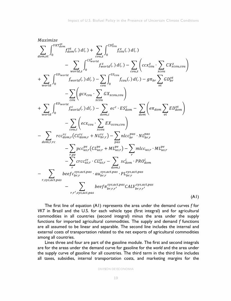
The first line of equation (A1) represents the area under the demand curves f for VKT in Brazil and the U.S. for each vehicle type (first integral) and for agricultural commodities in all countries (second integral) minus the area under the supply functions for imported agricultural commodities. The supply and demand f functions are all assumed to be linear and separable. The second line includes the internal and external costs of transportation related to the net exports of agricultural commodities among all countries.

Lines three and four are part of the gasoline module. The first and second integrals are for the areas under the demand curve for gasoline for the world and the area under the supply curve of gasoline for all countries. The third term in the third line includes all taxes, subsidies, internal transportation costs, and marketing margins for the


19


gasoline consumed in Brazil, while the fourth line includes the external costs associated with the transportation of net gasoline exports.

The fifth and sixth lines represent the ethanol sector in the objective function. The first integral is the area under the demand curve for ethanol for the world. The second term represents the cost of producing ethanol from each feedstock including the price of the co-product from that feedstock weighted by its co-product factor, where biofuel feedstocks includes sugarcane, corn, and cellulosic biomass. The third term includes all taxes, subsidies, internal transportation costs, and marketing margins for the ethanol demand in each country. The fuel demand in Brazil is disaggregated at state level and with a detailed module for fuel transportation (by trucking). The sixth line includes the external costs of transportation associated with ethanol exports.

The lines 7-8 are associated with crop production; the first term in line seven represents the cost of producing row crops in each region on existing croplands and new croplands in the Brazil component. Regions are 137 mesoregions in Brazil, 295 CRDs in the U.S., and 17 provinces in Argentina. The second term in the same line is the cost of converting new lands from pasture uses to cropland, where the cost depends on the three pasture types, namely ‘pasture planted in good condition’, ‘pasture planted degraded’ and ‘native pasture’. The third term in line seven is the cost of producing perennial crops on croplands and marginal lands, where the two perennial crops are miscanthus and switchgrass. The first term in line eight is the cost of converting marginal lands to cropland. The eighth line includes also the cost of collecting crop residue (i.e. corn stover and wheat straw) for conversion to biomass. The last term in line eight is the cost of processing soybean to soymeal and soy oil and sugar beets and sugarcane to sugar.

The last two lines in equation (A1) are related to the beef-cattle module in Brazil. The first term is the annual cost of raising beef-cattle, measured in animal units, which depends on the total amount of pasture land in each system, activity, and pasture type. The systems are the extensive and semi-intensive and the activities contain three ranching practices, namely finishing, complete cycle and weaning. The second term represents the transportation costs of calves from weaning to finishing ranches among regions depending also on the system, activity, and pasture type.

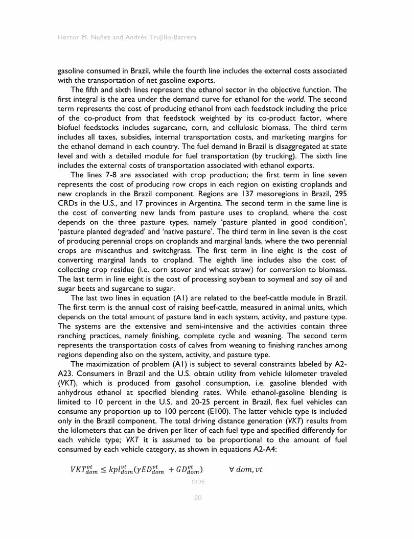
The maximization of problem (A1) is subject to several constraints labeled by A2-A23. Consumers in Brazil and the U.S. obtain utility from vehicle kilometer traveled (VKT), which is produced from gasohol consumption, i.e. gasoline blended with anhydrous ethanol at specified blending rates. While ethanol-gasoline blending is limited to 10 percent in the U.S. and 20-25 percent in Brazil, flex fuel vehicles can consume any proportion up to 100 percent (E100). The latter vehicle type is included only in the Brazil component. The total driving distance generation (VKT) results from the kilometers that can be driven per liter of each fuel type and specified differently for each vehicle type; VKT it is assumed to be proportional to the amount of fuel consumed by each vehicle category, as shown in equations A2-A4:

𝑉𝐾𝑇𝑑𝑜𝑚𝑣𝑡 ≤ 𝑘𝑝𝑙𝑑𝑜𝑚𝑣𝑡 (𝛾𝐸𝐷𝑑𝑜𝑚𝑣𝑡 + 𝐺𝐷𝑑𝑜𝑚𝑣𝑡 ) ∀ 𝑑𝑜𝑚, 𝑣𝑡

CIDE

20


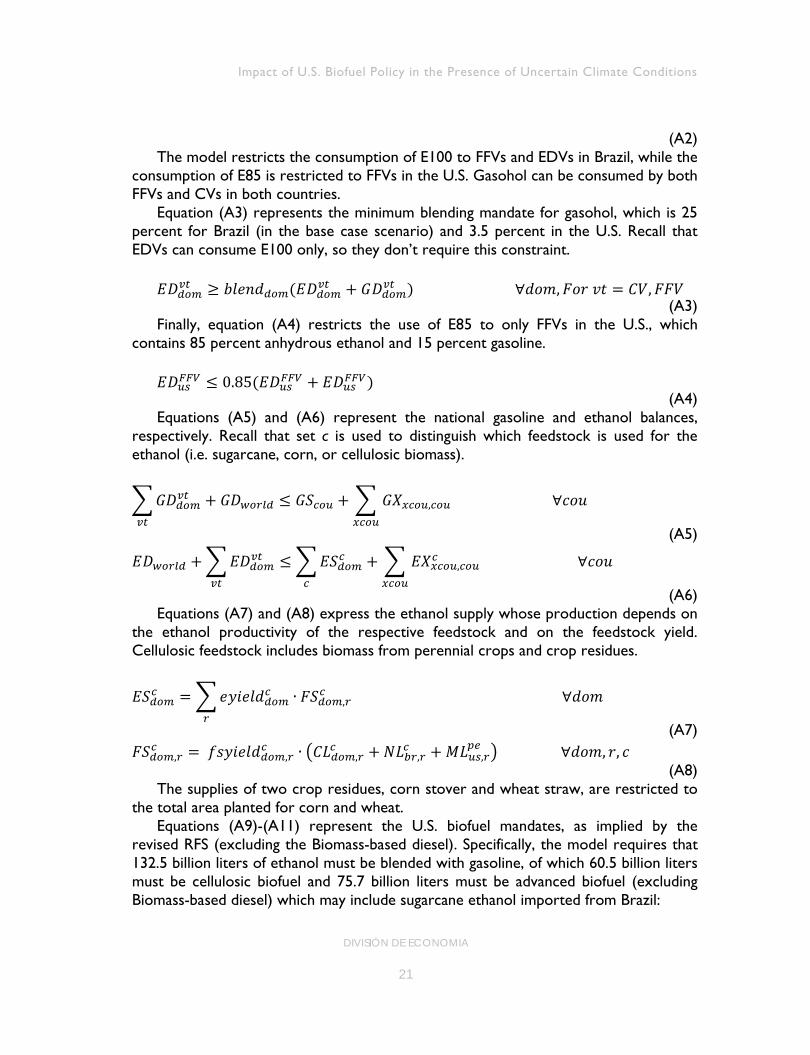
(A2) The model restricts the consumption of E100 to FFVs and EDVs in Brazil, while the

consumption of E85 is restricted to FFVs in the U.S. Gasohol can be consumed by both FFVs and CVs in both countries.

Equation (A3) represents the minimum blending mandate for gasohol, which is 25 percent for Brazil (in the base case scenario) and 3.5 percent in the U.S. Recall that EDVs can consume E100 only, so they don’t require this constraint.

𝐸𝐷𝑑𝑜𝑚𝑣𝑡 ≥ 𝑏𝑙𝑒𝑛𝑑𝑑𝑜𝑚(𝐸𝐷𝑑𝑜𝑚𝑣𝑡 + 𝐺𝐷𝑑𝑜𝑚𝑣𝑡 ) ∀𝑑𝑜𝑚,𝐹𝑜𝑟 𝑣𝑡 = 𝐶𝑉,𝐹𝐹𝑉

(A3) Finally, equation (A4) restricts the use of E85 to only FFVs in the U.S., which

contains 85 percent anhydrous ethanol and 15 percent gasoline. 𝐸𝐷𝑢𝑠𝐹𝐹𝑉 ≤ 0.85(𝐸𝐷𝑢𝑠𝐹𝐹𝑉 + 𝐸𝐷𝑢𝑠𝐹𝐹𝑉)

(A4) Equations (A5) and (A6) represent the national gasoline and ethanol balances,

respectively. Recall that set c is used to distinguish which feedstock is used for the ethanol (i.e. sugarcane, corn, or cellulosic biomass).

�𝐺𝐷𝑑𝑜𝑚𝑣𝑡

𝑣𝑡

+ 𝐺𝐷𝑤𝑜𝑟𝑙𝑑 ≤ 𝐺𝑆𝑐𝑜𝑢 + � 𝐺𝑋𝑥𝑐𝑜𝑢,𝑐𝑜𝑢𝑥𝑐𝑜𝑢

∀𝑐𝑜𝑢

(A5)

𝐸𝐷𝑤𝑜𝑟𝑙𝑑 + �𝐸𝐷𝑑𝑜𝑚𝑣𝑡

𝑣𝑡

≤�𝐸𝑆𝑑𝑜𝑚𝑐

𝑐

+ � 𝐸𝑋𝑥𝑐𝑜𝑢,𝑐𝑜𝑢𝑐

𝑥𝑐𝑜𝑢

∀𝑐𝑜𝑢

(A6) Equations (A7) and (A8) express the ethanol supply whose production depends on

the ethanol productivity of the respective feedstock and on the feedstock yield. Cellulosic feedstock includes biomass from perennial crops and crop residues.

𝐸𝑆𝑑𝑜𝑚𝑐 = �𝑒𝑦𝑖𝑒𝑙𝑑𝑑𝑜𝑚𝑐 ∙ 𝐹𝑆𝑑𝑜𝑚,𝑟𝑐

𝑟

∀𝑑𝑜𝑚

(A7) 𝐹𝑆𝑑𝑜𝑚,𝑟

𝑐 = 𝑓𝑠𝑦𝑖𝑒𝑙𝑑𝑑𝑜𝑚,𝑟𝑐 ∙ �𝐶𝐿𝑑𝑜𝑚,𝑟

𝑐 + 𝑁𝐿𝑏𝑟,𝑟𝑐 + 𝑀𝐿𝑢𝑠,𝑟

𝑝𝑒 � ∀𝑑𝑜𝑚, 𝑟, 𝑐 (A8)

The supplies of two crop residues, corn stover and wheat straw, are restricted to the total area planted for corn and wheat.

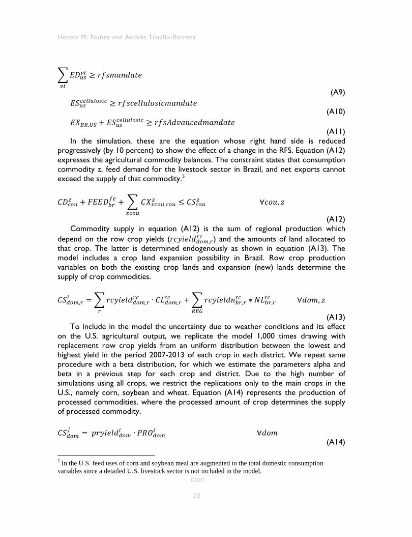
Equations (A9)-(A11) represent the U.S. biofuel mandates, as implied by the revised RFS (excluding the Biomass-based diesel). Specifically, the model requires that 132.5 billion liters of ethanol must be blended with gasoline, of which 60.5 billion liters must be cellulosic biofuel and 75.7 billion liters must be advanced biofuel (excluding Biomass-based diesel) which may include sugarcane ethanol imported from Brazil:


21


�𝐸𝐷𝑢𝑠𝑣𝑡𝑣𝑡

≥ 𝑟𝑓𝑠𝑚𝑎𝑛𝑑𝑎𝑡𝑒

(A9) 𝐸𝑆𝑢𝑠𝑐𝑒𝑙𝑙𝑢𝑙𝑜𝑠𝑖𝑐 ≥ 𝑟𝑓𝑠𝑐𝑒𝑙𝑙𝑢𝑙𝑜𝑠𝑖𝑐𝑚𝑎𝑛𝑑𝑎𝑡𝑒

(A10) 𝐸𝑋𝐵𝑅,𝑈𝑆 + 𝐸𝑆𝑢𝑠𝑐𝑒𝑙𝑙𝑢𝑙𝑜𝑠𝑖𝑐 ≥ 𝑟𝑓𝑠𝐴𝑑𝑣𝑎𝑛𝑐𝑒𝑑𝑚𝑎𝑛𝑑𝑎𝑡𝑒

(A11) In the simulation, these are the equation whose right hand side is reduced

progressively (by 10 percent) to show the effect of a change in the RFS. Equation (A12) expresses the agricultural commodity balances. The constraint states that consumption commodity z, feed demand for the livestock sector in Brazil, and net exports cannot exceed the supply of that commodity.5

𝐶𝐷𝑐𝑜𝑢𝑧 + 𝐹𝐸𝐸𝐷𝑏𝑟𝑓𝑒 + � 𝐶𝑋𝑥𝑐𝑜𝑢,𝑐𝑜𝑢

𝑧

𝑥𝑐𝑜𝑢

≤ 𝐶𝑆𝑐𝑜𝑢𝑧 ∀𝑐𝑜𝑢, 𝑧

(A12) Commodity supply in equation (A12) is the sum of regional production which

depend on the row crop yields (𝑟𝑐𝑦𝑖𝑒𝑙𝑑𝑑𝑜𝑚,𝑟𝑟𝑐 ) and the amounts of land allocated to

that crop. The latter is determined endogenously as shown in equation (A13). The model includes a crop land expansion possibility in Brazil. Row crop production variables on both the existing crop lands and expansion (new) lands determine the supply of crop commodities.

𝐶𝑆𝑑𝑜𝑚,𝑟𝑖 = �𝑟𝑐𝑦𝑖𝑒𝑙𝑑𝑑𝑜𝑚,𝑟

𝑟𝑐 ∙ 𝐶𝐿𝑑𝑜𝑚,𝑟𝑟𝑐

𝑟

+ �𝑟𝑐𝑦𝑖𝑒𝑙𝑑𝑛𝑏𝑟,𝑟rc ∗ 𝑁𝐿𝑏𝑟,𝑟

𝑟𝑐

𝑅𝐸𝐺

∀𝑑𝑜𝑚, 𝑧

(A13) To include in the model the uncertainty due to weather conditions and its effect

on the U.S. agricultural output, we replicate the model 1,000 times drawing with replacement row crop yields from an uniform distribution between the lowest and highest yield in the period 2007-2013 of each crop in each district. We repeat same procedure with a beta distribution, for which we estimate the parameters alpha and beta in a previous step for each crop and district. Due to the high number of simulations using all crops, we restrict the replications only to the main crops in the U.S., namely corn, soybean and wheat. Equation (A14) represents the production of processed commodities, where the processed amount of crop determines the supply of processed commodity.

𝐶𝑆𝑑𝑜𝑚

𝑗 = 𝑝𝑟𝑦𝑖𝑒𝑙𝑑𝑑𝑜𝑚𝑖 ∙ 𝑃𝑅𝑂𝑑𝑜𝑚𝑖 ∀𝑑𝑜𝑚 (A14)

5 In the U.S. feed uses of corn and soybean meal are augmented to the total domestic consumption variables since a detailed U.S. livestock sector is not included in the model.

CIDE

22


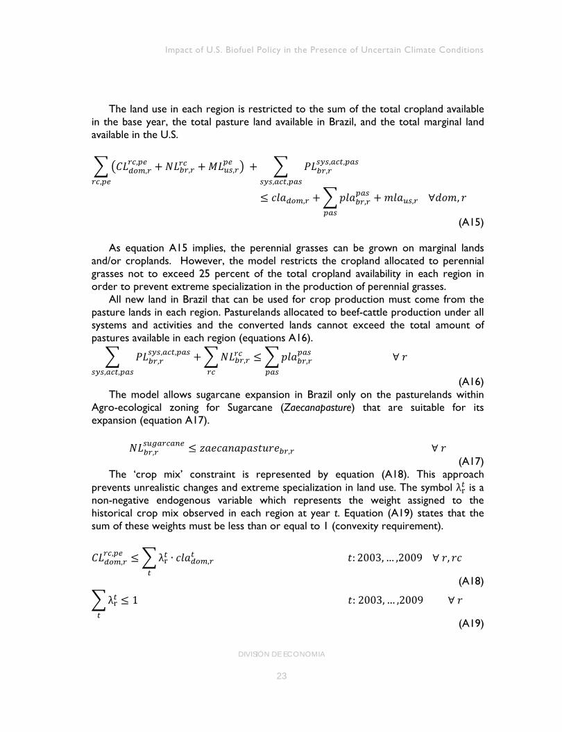
The land use in each region is restricted to the sum of the total cropland available

in the base year, the total pasture land available in Brazil, and the total marginal land available in the U.S.

��𝐶𝐿𝑑𝑜𝑚,𝑟𝑟𝑐,𝑝𝑒 + 𝑁𝐿𝑏𝑟,𝑟

𝑟𝑐 + 𝑀𝐿𝑢𝑠,𝑟𝑝𝑒 �

𝑟𝑐,𝑝𝑒

+ � 𝑃𝐿𝑏𝑟,𝑟𝑠𝑦𝑠,𝑎𝑐𝑡,𝑝𝑎𝑠


≤ 𝑐𝑙𝑎𝑑𝑜𝑚,𝑟 + �𝑝𝑙𝑎𝑏𝑟,𝑟𝑝𝑎𝑠

𝑝𝑎𝑠

+ 𝑚𝑙𝑎𝑢𝑠,𝑟 ∀𝑑𝑜𝑚, 𝑟

(A15)

As equation A15 implies, the perennial grasses can be grown on marginal lands and/or croplands. However, the model restricts the cropland allocated to perennial grasses not to exceed 25 percent of the total cropland availability in each region in order to prevent extreme specialization in the production of perennial grasses.

All new land in Brazil that can be used for crop production must come from the pasture lands in each region. Pasturelands allocated to beef-cattle production under all systems and activities and the converted lands cannot exceed the total amount of pastures available in each region (equations A16).

� 𝑃𝐿𝑏𝑟,𝑟𝑠𝑦𝑠,𝑎𝑐𝑡,𝑝𝑎𝑠


+ �𝑁𝐿𝑏𝑟,𝑟𝑟𝑐

𝑟𝑐

≤�𝑝𝑙𝑎𝑏𝑟,𝑟𝑝𝑎𝑠

𝑝𝑎𝑠

∀ 𝑟

(A16) The model allows sugarcane expansion in Brazil only on the pasturelands within

Agro-ecological zoning for Sugarcane (Zaecanapasture) that are suitable for its expansion (equation A17).

𝑁𝐿𝑏𝑟,𝑟

𝑠𝑢𝑔𝑎𝑟𝑐𝑎𝑛𝑒 ≤ 𝑧𝑎𝑒𝑐𝑎𝑛𝑎𝑝𝑎𝑠𝑡𝑢𝑟𝑒𝑏𝑟,𝑟 ∀ 𝑟 (A17)

The ‘crop mix’ constraint is represented by equation (A18). This approach prevents unrealistic changes and extreme specialization in land use. The symbol λr𝑡 is a non-negative endogenous variable which represents the weight assigned to the historical crop mix observed in each region at year t. Equation (A19) states that the sum of these weights must be less than or equal to 1 (convexity requirement).

𝐶𝐿𝑑𝑜𝑚,𝑟𝑟𝑐,𝑝𝑒 ≤�λr𝑡 ∙ 𝑐𝑙𝑎𝑑𝑜𝑚,𝑟

𝑡

𝑡

𝑡: 2003, … ,2009 ∀ 𝑟, 𝑟𝑐

(A18)

�λr𝑡𝑡

≤ 1 𝑡: 2003, … ,2009 ∀ 𝑟

(A19)


23


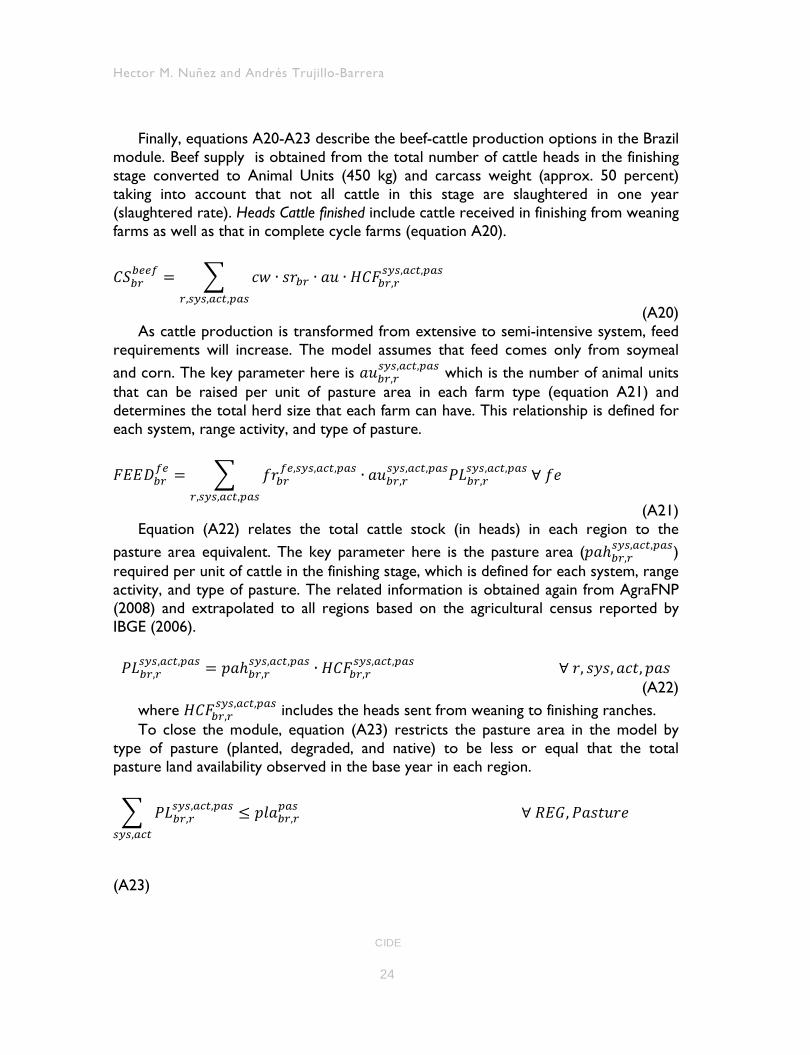
Finally, equations A20-A23 describe the beef-cattle production options in the Brazil module. Beef supply is obtained from the total number of cattle heads in the finishing stage converted to Animal Units (450 kg) and carcass weight (approx. 50 percent) taking into account that not all cattle in this stage are slaughtered in one year (slaughtered rate). Heads Cattle finished include cattle received in finishing from weaning farms as well as that in complete cycle farms (equation A20).

𝐶𝑆𝑏𝑟𝑏𝑒𝑒𝑓 = � 𝑐𝑤 ∙ 𝑠𝑟𝑏𝑟 ∙ 𝑎𝑢

𝑟,𝑠𝑦𝑠,𝑎𝑐𝑡,𝑝𝑎𝑠

∙ 𝐻𝐶𝐹𝑏𝑟,𝑟𝑠𝑦𝑠,𝑎𝑐𝑡,𝑝𝑎𝑠

(A20) As cattle production is transformed from extensive to semi-intensive system, feed

requirements will increase. The model assumes that feed comes only from soymeal and corn. The key parameter here is 𝑎𝑢𝑏𝑟,𝑟

𝑠𝑦𝑠,𝑎𝑐𝑡,𝑝𝑎𝑠 which is the number of animal units that can be raised per unit of pasture area in each farm type (equation A21) and determines the total herd size that each farm can have. This relationship is defined for each system, range activity, and type of pasture.

𝐹𝐸𝐸𝐷𝑏𝑟𝑓𝑒 = � 𝑓𝑟𝑏𝑟

𝑓𝑒,𝑠𝑦𝑠,𝑎𝑐𝑡,𝑝𝑎𝑠

𝑟,𝑠𝑦𝑠,𝑎𝑐𝑡,𝑝𝑎𝑠

∙ 𝑎𝑢𝑏𝑟,𝑟𝑠𝑦𝑠,𝑎𝑐𝑡,𝑝𝑎𝑠𝑃𝐿𝑏𝑟,𝑟

𝑠𝑦𝑠,𝑎𝑐𝑡,𝑝𝑎𝑠 ∀ 𝑓𝑒

(A21) Equation (A22) relates the total cattle stock (in heads) in each region to the

pasture area equivalent. The key parameter here is the pasture area (𝑝𝑎ℎ𝑏𝑟,𝑟𝑠𝑦𝑠,𝑎𝑐𝑡,𝑝𝑎𝑠)

required per unit of cattle in the finishing stage, which is defined for each system, range activity, and type of pasture. The related information is obtained again from AgraFNP (2008) and extrapolated to all regions based on the agricultural census reported by IBGE (2006).

𝑃𝐿𝑏𝑟,𝑟

𝑠𝑦𝑠,𝑎𝑐𝑡,𝑝𝑎𝑠 = 𝑝𝑎ℎ𝑏𝑟,𝑟𝑠𝑦𝑠,𝑎𝑐𝑡,𝑝𝑎𝑠 ∙ 𝐻𝐶𝐹𝑏𝑟,𝑟

𝑠𝑦𝑠,𝑎𝑐𝑡,𝑝𝑎𝑠 ∀ 𝑟, 𝑠𝑦𝑠,𝑎𝑐𝑡,𝑝𝑎𝑠 (A22)

where 𝐻𝐶𝐹𝑏𝑟,𝑟𝑠𝑦𝑠,𝑎𝑐𝑡,𝑝𝑎𝑠 includes the heads sent from weaning to finishing ranches.

To close the module, equation (A23) restricts the pasture area in the model by type of pasture (planted, degraded, and native) to be less or equal that the total pasture land availability observed in the base year in each region.

� 𝑃𝐿𝑏𝑟,𝑟𝑠𝑦𝑠,𝑎𝑐𝑡,𝑝𝑎𝑠

𝑠𝑦𝑠,𝑎𝑐𝑡

≤ 𝑝𝑙𝑎𝑏𝑟,𝑟𝑝𝑎𝑠 ∀ 𝑅𝐸𝐺,𝑃𝑎𝑠𝑡𝑢𝑟𝑒

(A23)

CIDE

24


References

AgraFNP. (2008). ANUALPEC, Anuario da Pecuária Brasileira. Babcock B. (2012). The impact of US biofuel policies on agricultural price levels

and volatility. China Agric. Econ. Rev. 4, 407 – 426. Babcock B, Zhou W. (2013). Impact on Corn Prices from Reduced Biofuel

Mandates. Center for Agricultural and Rural Development. 13 Working Paper 54. Accessed January 2014, available at http://www.card.iastate.edu/publications/dbs/pdffiles/13wp543.pdf

Babcock B. (2011). The Impact of US Biofuel Policies on Agricultural Price Levels and Volatility the Impact of US Biofuel Policies on Agricultural Price Levels and Volatility. ICTSD Programme on Agricultural Trade and Sustainable Development. 35. Accessed January 2014, available at http://www.ictsd.org/themes/agriculture/research/the-impact-of-us-biofuel-policies-on-agricultural-price-levels-and

Baffes J, Piot-Lepetit I, M’Barek R. (2011). Methods to analyse agricultural commodity price volatility. Ed. Isabelle Piot-Lepetit, Robert M’Barek. Springer New York. New York, NY.

Carter C, Rausser G, Smith A. (2012). The effect of the US ethanol mandate on corn prices. Department of Agricultural and Resource Economics. Accessed January 2014, available at http://agecon.ucdavis.edu/people/faculty/aaron-smith/docs/Carter_Rausser_Smith_Ethanol_Paper_Sep18.pdf

Claassen R, Just RE. 2011. Heterogeneity and Distributional Form of Farm-Level Yields. Am. J. Agric. Econ. 93,144–160.

Condon N, Klemick H, Wolverton A. (2013). Impacts of Ethanol Policy on Corn Prices: A Review and Meta-Analysis of Recent Evidence. Agricultural & Applied Economics Association. Washington, DC. Accessed September 2013, available at http://ageconsearch.umn.edu/bitstream/149940/2/Corn%20Ethanol%20and%20Food%20Prices%202013%20AAEA_submission.pdf

Energy Improvement and Extension Act. (2008). Public Law 110-343. Public Law. Energy Policy Act. 2005. 109th Congress. Public Law 109–58. Public Law. EPA. 2012. Notice of Decision Regarding Requests for a Waiver of the

Renewable Fuel Standard. Accessed January 2014, available at http://www.epa.gov/otaq/fuels/renewablefuels/documents/420f12075.pdf.

Fabiosa JF, Beghin JC, Dong F, Elobeid A, Tokgoz S, Yu T-H. (2010). Land allocation effects of the global ethanol surge: Predictions from the international FAPRI model. Land Econ. 86, 687–706.

Gilbert CL, Morgan CW. (2010). Food price volatility. Philos. Trans. R. Soc. Lond. B. Biol. Sci. 365,3023–34.

Hertel T, Tyner W, Birur D. (2010). The global impacts of biofuel mandates. Energy J.75–100.


25


Hochman G, Rajagopal D, Timilsina G, Zilberman D. (2011). The role of inventory adjustments in quantifying factors causing food price inflation. World Bank Policy Res. Work. Pap. Ser.

IBGE. (2006). Agricultural Census. Accessed October 2013, available at http://www.ibge.gov.br/home/estatistica/economia/agropecuaria/censoagro/default.shtm.

Mori K. (2012). Modeling the impact of a carbon tax: A trial analysis for Washington State. Energy Policy. 48, 627–639.

Norwood B, Roberts MC, Lusk JL. (2004). Ranking Crop Yield Models Using Out-of-Sample Likelihood Functions. Am. J. Agric. Econ. 86,1032–1043.

Nuñez HM, Önal H, Khanna M. (2013). Land use and economic effects of alternative biofuel policies in Brazil and the United States. Agric. Econ. 44,487–499.

Renewable Fuels Association. (2013). Industry Statistics. Accessed February 2014, available at http://www.ethanolrfa.org/pages/statistics.

Roberts MJ, Tran AN. (2013). Conditional Suspension of the US Ethanol Mandate using Threshold Price inside a Competitive Storage Model. Agricultural & Applied Economics Association. Washington, DC. Accessed September 2013, available at http://ageconsearch.umn.edu/bitstream/150717/2/AAEA2013_Tran.pdf

Searchinger T, Heimlich R, Houghton RA, Dong F, Elobeid A, Fabiosa J, Tokgoz S, Hayes D, Yu T-H. (2008). Use of U.S. croplands for biofuels increases greenhouse gases through emissions from land-use change. Science. 319, 1238–40.

Timilsina GR, Beghin JC, van der Mensbrugghe D, Mevel S. (2012). The impacts of biofuels targets on land-use change and food supply: A global CGE assessment. Agric. Econ. 43, 315–332.

Tokgoz S, Elobeid A, Fabiosa J, Hayes DJ, Babcock BA, Yu T-H (Edward), Dong F, Hart CE. (2008). Bottlenecks, Drought, and Oil Price Spikes: Impact on U.S. Ethanol and Agricultural Sectors. Rev. Agric. Econ. 30, 604–622.

Tyner W. (2010). The integration of energy and agricultural markets. Agric. Econ. 41,193–201.

Tyner W, Taheripour F, Hurt C. (2012). Potential Impacts of a Partial Waiver of the Ethanol Blending Rules. Farm Foundation. Purdue University. Accessed October 2013, available http://www.farmfoundation.org/news/articlefiles/1841-Purdue%20paper%20final%208-14-12.pdf

U.S. Farm Bill. (2008). 110th Congress. Public Law 110 – 246. Public Law:1–663. U.S. International Trade Comission. 2011. U.S. Tariff and Trade Data. USDA-ERS. (2012). Bioenergy: Background. US Deparment Agric. Accessed

November 2013, available at http://www.ers.usda.gov/topics/farm-economy/bioenergy/background.aspx.

CIDE

26


USDA-NASS. (2012). U.S. and State Data Quick Stats 2.0. Data Stat. Accessed November 2014, available at http://quickstats.nass.usda.gov/.

Woodard JD, Sherrick BJ. (2011). Estimation of Mixture Models using Cross-Validation Optimization: Implications for Crop Yield Distribution Modeling. Am. J. Agric. Econ. 93, 968–982.

Wright BD. (2011). The economics of grain price volatility. Appl. Econ. Perspect. Policy. 33, 32–58.

Yu T, Babcock BA. (2010). Are U.S. Corn and Soybeans Becoming More Drought Tolerant? Am. J. Agric. Econ. 92, 1310–1323.

Zilberman D, Hochman G, Rajagopal D, Sexton S, Timilsina G. 2012. The Impact of Biofuels on Commodity Food Prices: Assessment of Findings. Am. J. Agric. Econ. 95, 275–281


27

Documents

NÚÑEZ AND ANDRÉS TRUJILLO-BARRERA Impact of … · Impact of U.S. Biofuel Policy in the Presence of Drastic Climate Conditions . ... the markets to adjust to new ... out of methyl