NEXT-GENERATION TRANSIT SURVEYSECOND DATA RELEASE DOCUMENT

Data release description and supplemental information for thesecond public data release from the Next-Generation Transit

Survey (NGTS)

NGTS Consortium

July 20, 2020

http://ngtransits.org

ES

O

Sc

ie

nc

e

Ar

ch

iv

e

Fa

ci

li

ty

-

P

ha

se

3

D

at

a

Re

le

as

e

De

sc

ri

pt

io

n

ES

O p

rogr

amm

e T

he N

ext G

ener

atio

n T

rans

it S

urve

y, D

ata

Rel

ease

DR

2pr

ovid

ed b

y R

icha

rd W

est,

subm

itted

on

2020

-07-

02, p

ublis

hed

on 2

020-

07-2

0re

leas

e de

scrip

tion

docu

men

t rev

ised

on

2020

-07-

20

Contents

1 Overview of Observations 4

2 Previous Releases 6

3 Release Content 63.1 Overview . . . . . . . . . . . . . . . . . . . . . . . . . . . . . . . . . . . . . 63.2 Image Data Products . . . . . . . . . . . . . . . . . . . . . . . . . . . . . . 73.3 Source Catalogue . . . . . . . . . . . . . . . . . . . . . . . . . . . . . . . . 73.4 Lightcurves . . . . . . . . . . . . . . . . . . . . . . . . . . . . . . . . . . . 10

4 Release Notes 11

5 Data Reduction and Calibration 11

6 Data Quality 15

7 Acknowledgements 15

References 17

1

Acronyms

CCD Charged-Coupled Device

FOV Field of View

FWHM Full Width at Half Maximum

MCMC Markov chain Monte-Carlo

NGTS The Next-Generation Transit Survey

PSF Point-Spread Function

QE Quantum Efficiency

RMS Root Mean Square

SNR Signal-to-Noise Ratio

VLT Very Large Telescope

2

Abstract

The Next-Generation Transit Survey (NGTS) is a ground-based exoplanet sur-vey designed to detect and study Neptune and super-Earth sized planets aroundbright host stars using the transit method. The project is described by Wheatleyet al. (2018) and the project website is http://ngtransits.org.

The NGTS facility consists of 12 robotic telescopes situated at the EuropeanSouthern Observatory (ESO) site in Paranal, Chile. Each 20-cm, f/2.8 telescopehas a field-of-view of 2.8◦× 2.8◦ and is equipped with a custom NGTS filter and anAndor iKon-L 936 camera, which uses a deep-depletion CCD42-40 back-illuminatedCCD sensor.

During commissioning and the first two years of science observations, spanning21-Sep-2015 to 01-Apr-2018, NGTS observed 72 fields. A total of 110 982 662 788(1.1×1011) photometric measurements were made of 629 421 targets from 12 850 709images, taken at a cadence of 13 seconds. Each field was imaged between 64 000and 250 000 times. For each field, we have released an example science image, asource list with cross-matched identifiers from other surveys, a stacked frame fromwhich the source list was generated, and the detrended source lightcurves producedby aperture photometry. These data constitute NGTS Data Release 2 (DR2).

3

0h 21h 18h 15h 12h 9h 6h 3h 0h0°

30°

60°60°

30°

-30°

-60° -60°

-30°

Figure 1: The sky coverage of NGTS DR2. The intensity of the shading of each field isproportional to the number of images of that field.

1 Overview of Observations

A total of 72 fields measuring 2.8 × 2.8◦ are included in the second data release. Thesky coverage of NGTS DR2 is shown in Figure 1. These fields were observed over thecourse of two and a half years spanning the period 21-Sep-2015 to 01-Apr-2018. Fieldswere included in NGTS DR2 if the final date of observation was before 01-Apr-2018, thetwo-year cut-off for the data release marked from the start of routine survey operation on01-Apr-2016. Fields which were not completed during the second year will be included inthe next data release.

The individual object lightcurves were sampled at 13-second cadence, with a 10 secondexposure time, and contain between 64 000 and 250 000 data points depending on the field.Observations were conducted by the 12 NGTS telescopes, which are described in full byWheatley et al. (2018). Each telescope is fitted with a custom NGTS filter with a bandpassof 520–890 nm, which increases sensitivity to late-K and early-M stars. Figure 2 showsthe CCD QE, filter transmission curve and the expected throughput of the telescope.

Each telescope followed one field from when it rose above an elevation of 30◦ until when itset below 30◦. Once a field had set, another was picked up for the remainder of the night.Fields were chosen to minimize idle time, with each telescope typically observing 2 fieldsper night. Fields were selected from a discrete mesh of 5,307 mesh centers, and werechosen to maximize expected planetary yield, based on: the density of stars, expectednumber of dwarf stars, ecliptic latitude and the presence of bright stars or other extendedobjects in the field of view (FOV).

4

Figure 2: A plot showing the transmission curve of the custom NGTS filter, the measuredQE for the CCD chip and the telescope throughput. This plot is from Wheatley et al.(2018)

5

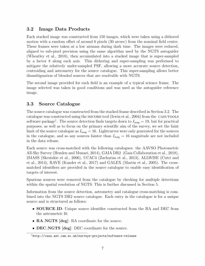
Table 1: Summary of the data products released for each NGTS field, where {FIELD}denotes the field name. The example science frame is a high-quality frame taken undergood conditions at low airmass. The dithered stack frame is a super-sampled image,constructed from a series images with dithered pointing, from which the source catalogueis derived. The source and lightcurve catalogues are, respectively, the source list and thephotometric lightcurves. The lightcurves for each field are separated on a 5 by 5 equal-sized grid and each tile is assigned a letter from A to Y. This is denoted by {LETTER}in the naming convention.

DataProduct

PRODCATG Keyword Naming Convention

ExampleScience Frame

ANCILLARY.IMAGE AG REFERENCE {FIELD}.fits

Dithered Stack SCIENCE.IMAGE DITHERED STACK {FIELD}.fitsSourceCatalogue

SCIENCE.CATALOGTILE SOURCE CATALOGUE {FIELD}.fits

LightcurveCatalogue

SCIENCE.CATALOGTILE FLUX {FIELD}{LETTER}.fits

The lightcurves were reduced via the usual procedure, using bias, dark and sky flat-fieldframes taken over the course of observations. Bias and dark frames were taken at dawnafter the telescopes had been stowed and the enclosure had been closed. Flat-field frameswere taken at dawn and dusk, when the weather was clear, and were carefully processedto remove clouds and stars.

2 Previous Releases

Since the first NGTS data release, NGTS DR1, we made improvements to our flat fielding,source detection and detrending techniques. Therefore we reprocessed all existing dataand, for uniformity, NGTS DR2 includes a new release of the 24 fields of NGTS DR1.

3 Release Content

3.1 Overview

NGTS DR2 consists of 4 data products as 28 separate files for each observed field. Thesedata products are summarised in Table 1, and consist of: an example high-quality scienceimage; a super-sampled stacked image; a source catalogue generated from the stackedimage; and the lightcurves of the objects in the source catalogue. For technical reasons,each field has been split into an equal 5x5 grid and the lightcurves are provided as 25separate files. In total the data release consists of 3.98 TB of data across 2018 files.

6

3.2 Image Data Products

Each stacked image was constructed from 150 images, which were taken using a ditheredmotion with a random offset of around 6 pixels (30 arcsec) from the nominal field centre.These frames were taken at a low airmass during dark time. The images were reduced,aligned to sub-pixel precision using the same algorithm used by the NGTS autoguider(Wheatley et al., 2018), then accumulated into a stacked image that is super-sampledby a factor 8 along each axis. This dithering and super-sampling was performed tomitigate the relatively under-sampled PSF, allowing a more accurate source detection,centroiding and astrometry for the source catalogue. This super-sampling allows betterdisambiguation of blended sources that are resolvable with NGTS.

The second image provided for each field is an example of a typical science frame. Theimage selected was taken in good conditions and was used as the autoguider referenceimage.

3.3 Source Catalogue

The source catalogue was constructed from the stacked frame described in Section 3.2. Thecatalogue was constructed using the imcore tool (Irwin et al., 2004) from the casutoolssoftware package1. The source detection finds targets down to Imag = 19, but for practicalpurposes, as well as to focus on the primary scientific aim of the survey, we set the faintlimit of the source catalogue as Imag = 16. Lightcurves were only generated for the sourcesin the catalogue, and so any sources fainter than Imag = 16 magnitude are not includedin the data release.

Each source was cross-matched with the following catalogues: the AAVSO PhotometricAll-Sky Survey (Henden and Munari, 2014), GAIA DR2 (Gaia Collaboration et al., 2018),2MASS (Skrutskie et al., 2006), UCAC4 (Zacharias et al., 2013), ALLWISE (Cutri andet al., 2014), RAVE (Kunder et al., 2017) and GALEX (Martin et al., 2005). The cross-matched identifiers are provided in the source catalogue to enable easy identification oftargets of interest.

Spurious sources were removed from the catalogue by checking for multiple detectionswithin the spatial resolution of NGTS. This is further discussed in Section 5.

Information from the source detection, astrometry and catalogue cross-matching is com-bined into the NGTS DR2 source catalogue. Each entry in the catalogue is for a uniquesource and is structured as follows:

• SOURCE ID: Unique source identifier constructed from the RA and DEC fromthe astrometric fit

• RA NGTS [deg]: RA coordinate for the source.

• DEC NGTS [deg]: DEC coordinate for the source.

1http://casu.ast.cam.ac.uk/surveys-projects/software-release

7

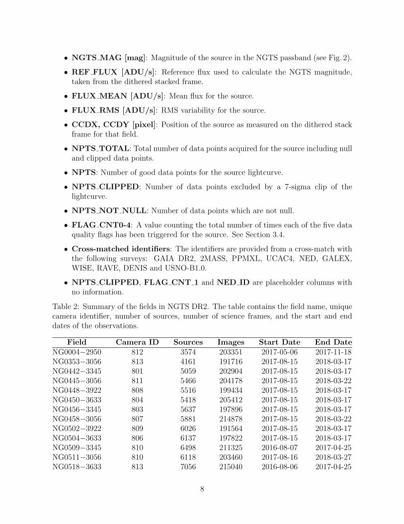
• NGTS MAG [mag]: Magnitude of the source in the NGTS passband (see Fig. 2).

• REF FLUX [ADU/s]: Reference flux used to calculate the NGTS magnitude,taken from the dithered stacked frame.

• FLUX MEAN [ADU/s]: Mean flux for the source.

• FLUX RMS [ADU/s]: RMS variability for the source.

• CCDX, CCDY [pixel]: Position of the source as measured on the dithered stackframe for that field.

• NPTS TOTAL: Total number of data points acquired for the source including nulland clipped data points.

• NPTS: Number of good data points for the source lightcurve.

• NPTS CLIPPED: Number of data points excluded by a 7-sigma clip of thelightcurve.

• NPTS NOT NULL: Number of data points which are not null.

• FLAG CNT0-4: A value counting the total number of times each of the five dataquality flags has been triggered for the source. See Section 3.4.

• Cross-matched identifiers: The identifiers are provided from a cross-match withthe following surveys: GAIA DR2, 2MASS, PPMXL, UCAC4, NED, GALEX,WISE, RAVE, DENIS and USNO-B1.0.

• NPTS CLIPPED, FLAG CNT 1 and NED ID are placeholder columns withno information.

Table 2: Summary of the fields in NGTS DR2. The table contains the field name, uniquecamera identifier, number of sources, number of science frames, and the start and enddates of the observations.

Field Camera ID Sources Images Start Date End DateNG0004−2950 812 3574 203351 2017-05-06 2017-11-18NG0353−3056 813 4161 191716 2017-08-15 2018-03-17NG0442−3345 801 5059 202904 2017-08-15 2018-03-17NG0445−3056 811 5466 204178 2017-08-15 2018-03-22NG0448−3922 808 5516 199434 2017-08-15 2018-03-17NG0450−3633 804 5418 205412 2017-08-15 2018-03-17NG0456−3345 803 5637 197896 2017-08-15 2018-03-17NG0458−3056 807 5881 214878 2017-08-15 2018-03-22NG0502−3922 809 6026 191564 2017-08-15 2018-03-17NG0504−3633 806 6137 197822 2017-08-15 2018-03-17NG0509−3345 810 6498 211325 2016-08-07 2017-04-25NG0511−3056 810 6118 203460 2017-08-16 2018-03-27NG0518−3633 813 7056 215040 2016-08-06 2017-04-25

8

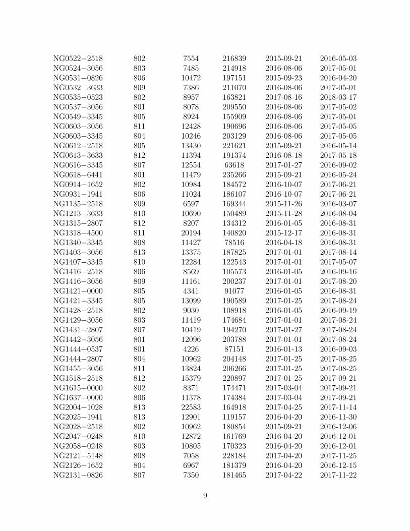
NG0522−2518 802 7554 216839 2015-09-21 2016-05-03NG0524−3056 803 7485 214918 2016-08-06 2017-05-01NG0531−0826 806 10472 197151 2015-09-23 2016-04-20NG0532−3633 809 7386 211070 2016-08-06 2017-05-01NG0535−0523 802 8957 163821 2017-08-16 2018-03-17NG0537−3056 801 8078 209550 2016-08-06 2017-05-02NG0549−3345 805 8924 155909 2016-08-06 2017-05-01NG0603−3056 811 12428 190696 2016-08-06 2017-05-05NG0603−3345 804 10246 203129 2016-08-06 2017-05-05NG0612−2518 805 13430 221621 2015-09-21 2016-05-14NG0613−3633 812 11394 191374 2016-08-18 2017-05-18NG0616−3345 807 12554 63618 2017-01-27 2016-09-02NG0618−6441 801 11479 235266 2015-09-21 2016-05-24NG0914−1652 802 10984 184572 2016-10-07 2017-06-21NG0931−1941 806 11024 186107 2016-10-07 2017-06-21NG1135−2518 809 6597 169344 2015-11-26 2016-03-07NG1213−3633 810 10690 150489 2015-11-28 2016-08-04NG1315−2807 812 8207 134312 2016-01-05 2016-08-31NG1318−4500 811 20194 140820 2015-12-17 2016-08-31NG1340−3345 808 11427 78516 2016-04-18 2016-08-31NG1403−3056 813 13375 187825 2017-01-01 2017-08-14NG1407−3345 810 12284 122543 2017-01-01 2017-05-07NG1416−2518 806 8569 105573 2016-01-05 2016-09-16NG1416−3056 809 11161 200237 2017-01-01 2017-08-20NG1421+0000 805 4341 91077 2016-01-05 2016-08-31NG1421−3345 805 13099 190589 2017-01-25 2017-08-24NG1428−2518 802 9030 108918 2016-01-05 2016-09-19NG1429−3056 803 11419 174684 2017-01-01 2017-08-24NG1431−2807 807 10419 194270 2017-01-27 2017-08-24NG1442−3056 801 12096 203788 2017-01-01 2017-08-24NG1444+0537 801 4226 87151 2016-01-13 2016-09-03NG1444−2807 804 10962 204148 2017-01-25 2017-08-25NG1455−3056 811 13824 206266 2017-01-25 2017-08-25NG1518−2518 812 15379 220897 2017-01-25 2017-09-21NG1615+0000 802 8371 174471 2017-03-04 2017-09-21NG1637+0000 806 11378 174384 2017-03-04 2017-09-21NG2004−1028 813 22583 164918 2017-04-25 2017-11-14NG2025−1941 813 12901 119157 2016-04-20 2016-11-30NG2028−2518 802 10962 180854 2015-09-21 2016-12-06NG2047−0248 810 12872 161769 2016-04-20 2016-12-01NG2058−0248 803 10805 170323 2016-04-20 2016-12-01NG2121−5148 808 7058 228184 2017-04-20 2017-11-25NG2126−1652 804 6967 181379 2016-04-20 2016-12-15NG2131−0826 807 7350 181465 2017-04-22 2017-11-22

9

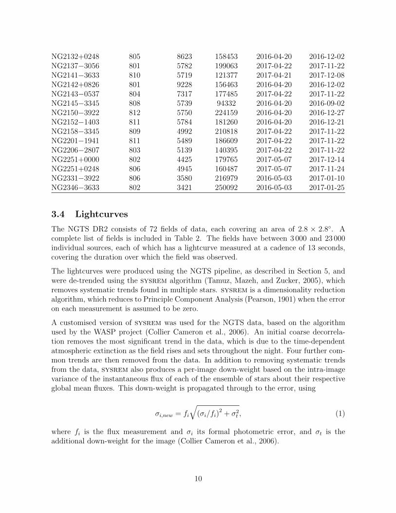
NG2132+0248 805 8623 158453 2016-04-20 2016-12-02NG2137−3056 801 5782 199063 2017-04-22 2017-11-22NG2141−3633 810 5719 121377 2017-04-21 2017-12-08NG2142+0826 801 9228 156463 2016-04-20 2016-12-02NG2143−0537 804 7317 177485 2017-04-22 2017-11-22NG2145−3345 808 5739 94332 2016-04-20 2016-09-02NG2150−3922 812 5750 224159 2016-04-20 2016-12-27NG2152−1403 811 5784 181260 2016-04-20 2016-12-21NG2158−3345 809 4992 210818 2017-04-22 2017-11-22NG2201−1941 811 5489 186609 2017-04-22 2017-11-22NG2206−2807 803 5139 140395 2017-04-22 2017-11-22NG2251+0000 802 4425 179765 2017-05-07 2017-12-14NG2251+0248 806 4945 160487 2017-05-07 2017-11-24NG2331−3922 806 3580 216979 2016-05-03 2017-01-10NG2346−3633 802 3421 250092 2016-05-03 2017-01-25

3.4 Lightcurves

The NGTS DR2 consists of 72 fields of data, each covering an area of 2.8 × 2.8◦. Acomplete list of fields is included in Table 2. The fields have between 3 000 and 23 000individual sources, each of which has a lightcurve measured at a cadence of 13 seconds,covering the duration over which the field was observed.

The lightcurves were produced using the NGTS pipeline, as described in Section 5, andwere de-trended using the sysrem algorithm (Tamuz, Mazeh, and Zucker, 2005), whichremoves systematic trends found in multiple stars. sysrem is a dimensionality reductionalgorithm, which reduces to Principle Component Analysis (Pearson, 1901) when the erroron each measurement is assumed to be zero.

A customised version of sysrem was used for the NGTS data, based on the algorithmused by the WASP project (Collier Cameron et al., 2006). An initial coarse decorrela-tion removes the most significant trend in the data, which is due to the time-dependentatmospheric extinction as the field rises and sets throughout the night. Four further com-mon trends are then removed from the data. In addition to removing systematic trendsfrom the data, sysrem also produces a per-image down-weight based on the intra-imagevariance of the instantaneous flux of each of the ensemble of stars about their respectiveglobal mean fluxes. This down-weight is propagated through to the error, using

σi,new = fi

√(σi/fi)

2 + σ2t , (1)

where fi is the flux measurement and σi its formal photometric error, and σt is theadditional down-weight for the image (Collier Cameron et al., 2006).

10

The final sysrem-corrected lightcurves are provided in the form of a catalogue. Ev-ery entry in the catalogue is a single photometric data point and contains the followinginformation:

• SOURCE ID: a unique identifier for each source constructed from it’s RA andDEC.

• HJD [days]: The time at which the measurement was taken, converted into HJD(UTC).

• SYSFLUX [ADU/s]: The sysrem-corrected flux measurement.

• FLUX ERROR [ADU/s]: The sysrem down-weighted error in the flux mea-surement.

• FLAG: The NGTS data quality flag.

Erroneous flux measurements produced by the pipeline were either set to ‘not a number’(NaN) or to zero. Additionally, the NGTS flagging system is used to identify data pointswhich are statistical outliers, or which may have been affected by bright stars, airplanescrossing the FOV or other contaminants such as the lasers used by the adaptive opticssystem of VLT UT4. Each flag consists of a single bit in an 8-bit integer which encodesa unique description of why the data point may have been flagged. The full list of flagscan be found in Table 3.

4 Release Notes

NGTS is a ground-based exoplanet survey designed to detect and study Neptune-size andsuper-Earth-size planets around bright host stars using the transit method. A detaileddescription of the project can be found in Wheatley et al. (2018). NGTS observes fieldsin a custom bandpass from 520–890 nm (Figure 2), which increases sensitivity to late-Kand early-M stars. NGTS achieves better than 1 mmag noise for most stars of Imag < 12in one hour of exposure time (Figure 3). Each NGTS image is calibrated using highquality bias and sky flat-field frames taken both before and after the science observations.Source detection is performed on a stack of dithered frames, designed to improve theaccuracy of the detection. Each image is solved astrometrically for accurate placement ofthe apertures used to perform photometry. The lightcurves are detrended using a customversion of the sysrem algorithm (Tamuz, Mazeh, and Zucker, 2005; Collier Cameronet al., 2006).

5 Data Reduction and Calibration

The NGTS pipeline takes raw images, both science and calibration, and produces high-quality detrended lightcurves for each detected source. The full structure of the pipeline is

11

Figure 3: A comparison of the measured fractional RMS noise level of a single NGTS fieldcompared with a theoretical model of the expected noise contributions. The NGTS datawere detrended and binned with a bin width of 1 hour. This plot is from Wheatley et al.(2018).

12

Table 3: Table describing the data quality flags employed by the NGTS pipepline toscreen for erroneous data points.

Flag Name Flag Description Bit

Saturation The maximum ADU in the aperture exceeds acamera-specific saturation threshold

bit 0

Cosmic Flagged if a cosmic ray has hit the CCD in theaperture

bit 1

Crossing Aperture is intersected by a large pixel-connectedregion above threshold which also intersects at leasttwo boundaries of the image (most commonly the VLTlaser system).

bit 2

Outlier The data point is found to be a > 7σ outlier bit 3Spike Aperture is intersected by a connected-pixel region

that contains pixels above saturation (most commonlyblooming spikes from neighbouring bright stars)

bit 4

Pipeline overview (CYCLE1807)

RefCatPipePhotPipe

MergePipe

SysremPipe

BLSPipe

BiasPipe

DarkPipe

FlatPipe

CalPipe

opis

DecorrPipe

DistortPipe

AutovetPipe

Figure 4: A schematic illustration of the NGTS photometric pipeline. Each box representsa distinct component in the NGTS pipeline and a single step in the processing of the data.BiasPipe, DarkPipe, FlatPipe and CalPipe are responsible for the production of highquality bias, dark and flat-field calibration frames. DistortPipe and RefCatPipe producethe astrometric calibration and source catalogue respectively. PhotPipe, MergePipe andSysremPipe produce the raw and then detrended lightcurves.

13

shown in Figure 4 as a schematic diagram. The calibration frames are processed throughBiasPipe, DarkPipe and FlatPipe and then through Calpipe to produce high-quality mas-ter frames.

PhotPipe processes the science images, performing image reduction, astrometry and aper-ture photometry. Each science frame is trimmed to remove the overscan and then is biasand flat-field corrected in the usual way. A model of the radial distortion of the telescopeis calculated once for each field using a custom MCMC code (DistortPipe). A 7th orderpolynomical is used with the distortion described by the 3rd, 5th and 7th order terms(Wheatley et al., 2018). The distortion is stable over time, and it is only updated whenany changes are made to the telescope hardware (e.g. for replacement of camera shutters).PhotPipe solves each image astrometrically so that apertures can be placed accurately.Each image is background-subtracted by calculating an interpolated value for the back-ground on a 64 by 64 pixel grid using a k-sigma clipped median. This improves the SNRof the background measurement while preserving some of the local structure.

MergePipe collates the raw photometry for each field into a single data product covering afull observing season, which is then passed through SysremPipe to produce the correctedlightcurves that make up the bulk of NGTS DR2. The detrending algorithm employed bySysremPipe is described in section 3.4. It is a custom version of the sysrem algorithm(Tamuz, Mazeh, and Zucker, 2005; Collier Cameron et al., 2006).

Source Catalogue

The source detection is run using the imcore tool from the casutools software package(Irwin et al., 2004). It is run on the dithered stacked frame from the field in order tobetter sample the stellar profile and produce more accurate source positions.

Astrometric Solution

For each science image, an astrometric solution is found in order to accurately placephotometric apertures on each source. The NGTS telescopes have a non-linear radialdistortion, and so a zenith polynomial projection is used (Calabretta and Greisen, 2002).The radial distortion is measured once for each field using a custom MCMC code (Dis-tortPipe), and this only updated if telescope hardware maintenance is carried out. A 7thorder polynomical is used with the distortion described by the 3rd, 5th and 7th orderterms (Wheatley et al., 2018). The per image astrometric solutions account for rotationand translation, as well as shear arising from atmospheric refraction.

Photometry

NGTS photometry is performed using the imcore package with a 3-pixel radius, soft-edged aperture, which is placed at the source position based on the derived astrometricsolution. The PSF FWHM is approximately 1.6–1.8 pixels and so less than 1% of light islost due to the finite aperture size. The NGTS pipeline performs only relative photometryas an absolute photometric calibration is not necessary for the primary science goal of

14

the survey. No explicit corrections are applied to the photometric measurements due toseeing variations over time as, given the pixel scale and size of the photometric apertureused, the effects of variable seeing are minimal.

6 Data Quality

Various data quality checks are carried out automatically within the calibration steps,particularly for flat-field frames, to reject saturated frames, frames afflicted by clouds andframes containing residual stars. In addition, all master calibration frames (from CalPipe)are visually inspected for quality and checked with statistical tests.

A full astrometric calibration is performed on each autoguider reference image, includingterms that describe the optical distortions. PhotPipe uses the appropriate DistortPipeparameters as an initial guess of the astrometric solution for each science image. Theastrometric fitting in PhotPipe only varies the WCS parameters that encode the pointingposition (including rotation), but not the distortion. The RMS error of the DistortPipefit is recorded and if this value is above a pre-determined threshold then PhotPipe fallsback on the astrometric solution from RefCatPipe, which was used during compilation ofthe source catalogue. Although the best result for each astrometric fit is assured, fittingis carried out on a field-by-field basis and residuals may vary by camera and by field.

During compilation of the source catalogue in RefCatPipe, contamination due to spuriousobjects is mitigated by cross-matching the results from the source detection with theexternal catalogues listed in Section 3.3. We place empirically defined limits on colourand separation to improve the accuracy of the cross-matching and screened for knownvariable stars and extra-galactic sources. The Gaia cross-match is used to determinewhether each NGTS source is a single object or a blend that is unresolved in NGTSimages. Objects fainter than 16th magnitude in the NGTS passband are cut from thecatalogue, thus this is the completeness limit at the faint end. RefCatPipe outputs aremanually checked for quality assurance.

The quality of the final photometry is assessed both visually and via statistical metrics,e.g. by comparing fractional RMS flux vs stellar magnitude, see Figure 3. Each flux datapoint has an associated data quality flag; see Section 3.4 for a full description.

7 Acknowledgements

Any publications making use of these data, whether obtained from the ESO archive orvia third parties, must include the following acknowledgement: “Based on data collectedunder the NGTS Project at the ESO La Silla Paranal Observatory.”

If the access to the ESO Science Archive Facility services was helpful for your research,please include the following acknowledgment: “This research has made use of the servicesof the ESO Science Archive Facility.”

15

Science data products from the ESO archive may be distributed by third parties, anddisseminated via other services, according to the terms of the Creative Commons Attri-bution 4.0 International license. Credit to ESO and the NGTS project as the origin ofthe data must be acknowledged, and the file headers preserved.

The NGTS facility is operated by the consortium institutes with support from the UK Sci-ence and Technology Facilities Council (STFC) project ST/M001962/1 and ST/S002642/1.The contributions at the University of Warwick have been supported by STFC throughconsolidated grants ST/L000733/1 and ST/P000495/1. Contributions at the Universityof Geneva were carried out within the framework of the National Centre for Competencein Research “PlanetS” supported by the Swiss National Science Foundation (SNSF). Thecontributions at the University of Leicester have been supported by STFC through con-solidated grant ST/N000757/1. Contributions at DLR have been supported by the DFGpriority program SPP 1992 “Exploring the Diversity of Extrasolar Planets” (RA 714/13-1).

16

References

Calabretta, M. R. and E. W. Greisen (Dec. 2002). “Representations of celestial coordinatesin FITS”. In: A&A 395, pp. 1077–1122. doi: 10.1051/0004-6361:20021327. arXiv:astro-ph/0207413 [astro-ph].

Collier Cameron, A. et al. (2006). “A fast hybrid algorithm for exoplanetary transitsearches”. In: Monthly Notices of the Royal Astronomical Society 373.2, pp. 799–810.doi: 10.1111/j.1365- 2966.2006.11074.x. eprint: /oup/backfile/content_

public / journal / mnras / 373 / 2 / 10 . 1111 / j . 1365 - 2966 . 2006 . 11074 . x / 2 /

mnras0373-0799.pdf. url: http://dx.doi.org/10.1111/j.1365-2966.2006.11074.x.

Cutri, R. M. and et al. (Jan. 2014). “VizieR Online Data Catalog: AllWISE Data Release(Cutri+ 2013)”. In: VizieR Online Data Catalog 2328.

Gaia Collaboration et al. (Aug. 2018). “Gaia Data Release 2. Summary of the contentsand survey properties”. In: A&A 616, A1, A1. doi: 10.1051/0004-6361/201833051.arXiv: 1804.09365 [astro-ph.GA].

Henden, A. and U. Munari (Mar. 2014). “The APASS all-sky, multi-epoch BVgri photo-metric survey”. In: Contributions of the Astronomical Observatory Skalnate Pleso 43,pp. 518–522.

Irwin, Mike J. et al. (2004). VISTA data flow system: pipeline processing for WFCAMand VISTA. doi: 10.1117/12.551449. url: https://doi.org/10.1117/12.551449.

Kunder, A. et al. (Feb. 2017). “The Radial Velocity Experiment (RAVE): Fifth DataRelease”. In: AJ 153, 75, p. 75. doi: 10.3847/1538-3881/153/2/75. arXiv: 1609.03210 [astro-ph.SR].

Martin, D. C. et al. (Jan. 2005). “The Galaxy Evolution Explorer: A Space UltravioletSurvey Mission”. In: ApJ 619, pp. L1–L6. doi: 10 . 1086 / 426387. eprint: astro -

ph/0411302.Pearson, K (1901). “LIII. On lines and planes of closest fit to systems of points in space”.

In: The London, Edinburgh, and Dublin Philosophical Magazine and Journal of Science2.11, pp. 559–572. doi: 10.1080/14786440109462720. eprint: https://doi.org/10.1080/14786440109462720. url: https://doi.org/10.1080/14786440109462720.

Skrutskie, M. F. et al. (Feb. 2006). “The Two Micron All Sky Survey (2MASS)”. In: AJ131, pp. 1163–1183. doi: 10.1086/498708.

Tamuz, O., T. Mazeh, and S. Zucker (Feb. 2005). “Correcting systematic effects in a largeset of photometric light curves”. In: mnras 356, pp. 1466–1470. doi: 10.1111/j.1365-2966.2004.08585.x. eprint: astro-ph/0502056.

Wheatley, P. J. et al. (Apr. 2018). “The Next Generation Transit Survey (NGTS)”. In:MNRAS 475, pp. 4476–4493. doi: 10 . 1093 / mnras / stx2836. arXiv: 1710 . 11100

[astro-ph.EP].Zacharias, N. et al. (Feb. 2013). “The Fourth US Naval Observatory CCD Astrograph

Catalog (UCAC4)”. In: AJ 145, 44, p. 44. doi: 10.1088/0004-6256/145/2/44. arXiv:1212.6182 [astro-ph.IM].

17