Next generation of refrigerants for residential heat pump ...Next generation of refrigerants for residential heat pump systems Martina Longhini ... as thermodynamic characteristics

Next generation of refrigerants for residential heat pump

systems

Martina Longhini

Thesis to obtain the Master of Science Degree in

Energy Engineering and Management

Supervisors: Prof. Luís Filipe Moreira Mendes

Dr. Hatef Madani Larijani

Examination Committee:

Chairperson: Prof. José Alberto Caiado Falcão de Campos

Supervisor: Prof. Luís Filipe Moreira Mendes

Member of the Committee: Dr. Ana Sofia Oliveira Henriques Moita

September 2015

i

Abstract

The increasing concentration of greenhouse gases (GHG) in the atmosphere arising from human

activities is unquestionably taking its toll on the environment with severe consequences that cannot be

ignored. It is therefore necessary to take measures to avoid or reduce GHG production and release. In

this scope, the 2015 F-gas regulation aims at limiting the contribution of the refrigeration industry to the

global warming effect by phasing-down refrigerants with high global warming potential (GWP).

This work contributes to this effort by analysing a number of refrigerants, i.e. R32, R152a, R290, R1270,

R1234yf and R1234ze(E) that could substitute the current R410A in a 10 kW domestic heat pump

typically used in a single family house in Sweden.

An EES model was thus created and the relevant outputs chosen to compare the refrigerants’ options

are the volumetric heating capacity, the coefficient of performance (COP), Seasonal coefficient of

performance (SCOP) – obtained by the method found in the Standard BS EN 14825:2012, the discharge

temperature, and the Total Equivalent Warming Impact (TEWI) factor.

The reductions observed for TEWI are remarkable. The overall lowest TEWI is obtained by refrigerants

having the lowest GWPs, i.e. the HCs, of 54.2% and 54.6% for R1270 and R290 respectively. They are

followed by R1234yf and R1234ze(E), with reductions of 52.5% and 53.7% respectively. R152a entails

a reduction of 53.6%, due to its higher SCOP. R32 shows a reduction of 40.8%. Other parameters such

as thermodynamic characteristics and safety issues are also considered during the analysis.

Keywords—CO2, GHG, Heat pump, R410A, refrigerant, TEWI

ii

Resumo

O aumento da concentração de gases de efeito de estufa (GHG) na atmosfera devido às atividades

humanas é inquestionável, com consequências ambientais que não podem ser ignoradas (Andres,

2012). É por isso importante implementar medidas para reduzir e evitar a produção e libertação de

GHG. Neste sentido, a regulamentação 2015 F-gas tem por objetivo limitar a contribuição da industria

da refrigeração para o aquecimento global, retirando dos equipamentos os frigorigéneos com maior

potencial de aquecimento global (GWP).

Esta tese pretendeu contribuir para este esforço, analisando-se vários fluidos - R32, R152a, R290,

R1270, R1234yf and R1234ze(E) - que possam substituir o R410A numa bomba de calor para uso

domestico de 10 kW, produzida na Suécia. Foi desenvolvido um modelo no programa EES de acordo

com a norma BS EN 14825:2012 e os parâmetros escolhidos para comparar os fluidos foram a potência

volumétrica, o COP nominal e sazonal (SCOP), a temperatura de descarga do compressor e, o mais

importante, o impacto total equivalente para o aquecimento global (TEWI).

As reduções do TEWI foram assinaláveis, sendo as TEWI mais baixas observadas para os

frigorigéneos com o menor GWP, os HCs, com -54,2% e -54,6% para o R1270 e o R290,

respetivamente. Também os frigorigéneos R1234yf e R1234ze(E) mostram uma redução assinalável,

respetivamente de -52,5% e -53,7%. O R152a apresenta uma redução de -53,6% devido ao seu

elevado SCOP. O R32 apresenta uma redução de 40,8%. Na análise foram ainda considerados outros

fatores importantes tais como as suas propriedades termodinâmicas e questões de segurança.

Palavras-chave—CO2, GHG, bomba de calor, R410A, refrigerante, TEWI

iii

Acknowledgements

First of all, I would like to thank Thermia for giving me the opportunity of performing this Thesis, and for

providing the data to start with.

A big thank you also goes to my supervisors, Prof. Hatef Madani in KTH and Prof. Filipe Mendes in IST,

for all the help they have given me during the semester. This is also true for Pavel, who I could call any

time I had a concern.

Finally I have to thank all the friends at the department of Energy at KTH for making the days of work at

the office not only about work but also about friendship and fun (and tennis table).

iv

Table of contents

1. Introduction ...................................................................................................................................... 1

1.1. Objectives and methodology ................................................................................................... 3

1.2. Scope and limitations .............................................................. Error! Bookmark not defined.

1.3. Thesis’ structure ...................................................................................................................... 4

2. Refrigerants ..................................................................................................................................... 5

2.1. Introductory concepts .............................................................................................................. 5

2.2. Characterisation of refrigerants ............................................................................................... 7

2.3. State of the art of the fourth generation’s refrigerants ........................................................... 13

2.3.1. HFCs .............................................................................................................................. 13

2.3.2. Natural Refrigerants....................................................................................................... 14

2.3.3. HCs ................................................................................................................................ 15

2.3.4. HFOs ............................................................................................................................. 16

2.4. Selected refrigerants for further analysis ............................................................................... 17

3. Analysis of the developed model ................................................................................................... 21

3.1. Heat pump model .................................................................................................................. 21

3.1.1. Basic assumptions ......................................................................................................... 23

3.1.2. Evaporator ..................................................................................................................... 24

3.1.3. Compressor ................................................................................................................... 26

3.1.4. Condenser ..................................................................................................................... 27

3.1.5. Expansion valve ............................................................................................................. 28

3.2. SCOP calculation................................................................................................................... 29

3.3. TEWI calculation .................................................................................................................... 31

4. Results and discussion .................................................................................................................. 33

4.1. Discharge temperature .......................................................................................................... 33

4.2. Heating capacity .................................................................................................................... 34

4.3. Coefficient of performance (COP) ......................................................................................... 35

4.4. Seasonal coefficient of performance (SCOP) ....................................................................... 38

4.5. Total equivalent warming impact (TEWI) .............................................................................. 40

4.5.1. Results ........................................................................................................................... 40

4.5.2. Sensitivity analysis ......................................................................................................... 42

4.6. Summary of results for each refrigerant ................................................................................ 45

4.6.1. R32 ................................................................................................................................ 47

4.6.2. R152a ............................................................................................................................ 47

4.6.3. R290 .............................................................................................................................. 48

4.6.4. R1270 ............................................................................................................................ 49

4.6.5. R1234yf ......................................................................................................................... 49

4.6.6. R1234ze(E) .................................................................................................................... 50

5. Conclusions and further work ........................................................................................................ 51

Bibliography ........................................................................................................................................... 53

APPENDIX .................................................................................................................................................i

v

List of figures

Figure 1.1. Greenhouse gas emissions saved by 2013 heat pump stock, by country (in Mt) (ehpa, 2014)

................................................................................................................. Error! Bookmark not defined.

Figure 1.2. Phase-down of fluorinated gases’ progress in time (Bitzer, 2014) ....................................... 2

Figure 2.1. Evolution of refrigerants in time (Danfoss, 2014) .................................................................. 6 Figure 2.2. Saturated vapour pressure vs. temperature ......................................................................... 8 Figure 2.3. Condenser (right) and evaporator (left) temperature profiles (SWEP International AB, 2012)

................................................................................................................................................................. 9 Figure 2.4. Pareto front (x) for the simple vapour compression cycle (air conditioned application)

(McLinden, 2014) ................................................................................................................................... 10 Figure 2.5. Pressure and operation criteria ........................................................................................... 18 Figure 2.6. Selected alternatives to R410A ........................................................................................... 19

Figure 3.1. Heat pump system .............................................................................................................. 21 Figure 3.2. Vapour compression cycle in log(p)-h diagram (left) and T-s diagram (right) ..................... 22

Figure 3.3. Temperature profiles of brine and refrigerant in the evaporator ......................................... 24 Figure 3.4. Isentropic efficiency of compressor for different refrigerants .............................................. 26

Figure 3.5. Temperature profiles of water and refrigerant in the condenser ......................................... 27 Figure 3.6. Temperature and heating demand profiles in colder climate scenario (BSI, 2012) ............ 30 Figure 4.1. Discharge temperature vs. outdoor temperature (radiator heating) .................................... 33

Figure 4.2. Volumetric heating capacity vs. outdoor temperature (radiator heating) ............................ 34 Figure 4.3. Volumetric heating capacity vs. outdoor temperature (floor heating) ................................. 35

Figure 4.4. COP vs. outdoor temperature (radiator heating) ................................................................. 36 Figure 4.5. COP vs. outdoor temperature (floor heating) ...................................................................... 37 Figure 4.6. SCOP by refrigerant over the heating season for colder climate scenario (radiator and floor

heating) .................................................................................................................................................. 38 Figure 4.7. Relative differences (%) of SCOP compared to R410A (radiator heating) ......................... 39

Figure 4.8. Relative differences (%) of SCOP compared to R410A (floor heating) .............................. 39 Figure 4.9. Figure 4.9. TEWI - Direct and indirect effect (radiator heating) .......................................... 40 Figure 4.10. Relative difference (%) of TEWI compared to R410A (radiator heating) .......................... 41

Figure 4.11. TEWI - Direct and indirect effect (floor heating) ................................................................ 41 Figure 4.12. Relative differences (%) of TEWI compared to R410A (floor heating) ............................. 42

Figure 4.13. Leakage rate sensitivity analysis results on TEWI ............................................................ 42 Figure 4.14. Lifetime sensitivity analysis on TEWI ................................................................................ 43 Figure 4.15. Recovery efficiency sensitivity analysis on TEWI ............................................................. 44

Figure 4.16. TEWI calculated with ENTSO-E grid average .................................................................. 45 Figure 4.17. Relative difference (%) of COP vs. relative difference (%) of VHC compared to R410A at

operating conditions corresponding to outdoor T ranging from -22 °C to 16 °C. .................................. 46 Figure 4.18. Summary of evaluated parameters for R32 ...................................................................... 47 Figure 4.19. Summary of evaluated parameters for R152a .................................................................. 48

Figure 4.20. Summary of evaluated parameters for R290 .................................................................... 48 Figure 4.21. Summary of evaluated parameters for R1270 .................................................................. 49

Figure 4.22. Summary of evaluated parameters for R1234yf ............................................................... 50 Figure 4.23. Summary of evaluated parameters for R1234ze(E) ......................................................... 50

vi

List of tables

Table 1.1. New products and equipment: F-gas ban summary table (Gluckman consulting, 2014) ...... 3

Table 2.1. Characteristics of the alternative refrigerants to R410A ....................................................... 19 Table 3.2. Input data .............................................................................................................................. 24

Table 3.3. Requirement for secondary fluid temperatures (BSI, 2012) ................................................. 30 Table 3.4. TEWI input parameters ........................................................................................................ 31 Table 3.5. Charge values by refrigerant ................................................................................................ 32

vii

Nomenclature

COP1 Coefficient of performance (heating mode) [-]

COP2 Coefficient of performance (cooling mode) [-]

CFC Chlorofluorocarbon

cp Specific heat capacity [kJ/kg-K]

Eannual Annual energy consumption [kWh/year]

elbu Electric back-up [kW]

F-gas Fluorinated gas

F-gas regulation

Regulation of the European Parliament and of the

Council on fluorinated gases and repealing Regulation

(EC) No 842/2006

FC Fluorocarbon

GWP Global warming potential

h1 Enthalpy at inlet of evaporator [J/kg]

h2 Enthalpy at outlet of evaporator/inlet compressor [J/kg]

h3 Enthalpy at outlet compressor/inlet condenser [J/kg]

h3,is Enthalpy at outlet compressor (isenthalpic process) [J/kg]

h4 Enthalpy at outlet condenser/inlet expansion valve [J/kg]

HC Hydrocarbon

HCFC Hydrochlorofluorocarbon

HFC Hydrofluorocarbon

HFO Hydrofluoroolefin

HP Heat pump

k Thermal conductivity [W/m-°C]

Lannual Annual leakage rate [kgref/year]

LMTD Logarithmic mean temperature difference [°C]

�̇�/�̇�𝒓𝒆𝒇 Mass flow rate/mass flow rate of refrigerant [kg/s]

m Refrigerant charge [kg]

N Lifetime of system [years]

ODP Ozone depletion potential

P Pressure [kPa]

Pratio Pressure ratio [-]

q1 Specific heating capacity [J/kg]

�̇�𝟏 Heating capacity [kW]

SCOP Season coefficient of performance [-]

T Temperature [°C]

TEWI Total equivalent warming impact [kg CO2]

�̇�𝒔𝒘𝒆𝒑𝒕 Swept volume [m3/s]

VHC Volumetric heating capacity [kJ/m3]

w Compressor specific work [J/kg]

wid Ideal required specific work [J/kg]

�̇� Compressor power [kW]

Greek characters

αrecovery Recovery efficiency of refrigerant [-]

β CO2 emission factor [kgCO2/kWh]

ηk Efficiency of compressor [-]

ηs Volumetric efficiency [-]

μ Dynamic viscosity [Pa/s]

ρ Density [kg/m3]

viii

Subscripts

1 Inlet evaporator/outlet expansion valve

2 Outlet evaporator/inlet compressor

3 Outlet compressor/inlet condenser

4 Outlet condenser/inlet expansion valve

j Temperature bin

-1-

1. Introduction

Carbon dioxide (CO2) emissions in the atmosphere arising from human doings, such as power

production from combustion of fossil fuels, industrial activities and – in the matter in question –

refrigeration, have become more of a concern as a result of their growing scale in the past decades.

The increasing concentration of greenhouse gases (GHG) is taking its toll on the environment with

severe consequences that cannot be ignored (Andres, 2012). It is therefore necessary to take measures

to avoid or reduce GHG production and release.

In this instance, heat pumps (HP) come forward as an increasingly important player. In fact, they

generally entail a lower electricity consumption when compared to equivalent electric radiator systems

thus emitting less GHG; the magnitude of their benefit highly depends on the local energy mix used for

electricity production (Forsén, 2005). Moreover, their impact is principally related to the refrigerant used,

as it affects the CO2 emissions of the system both directly and indirectly. As the number of installed

heat pump systems increases in a high number of countries worldwide, the importance of operating

with a low impacting refrigerant becomes crucial.

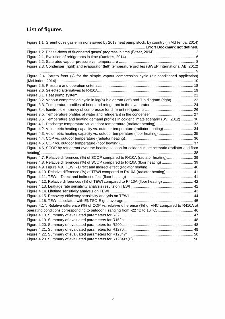
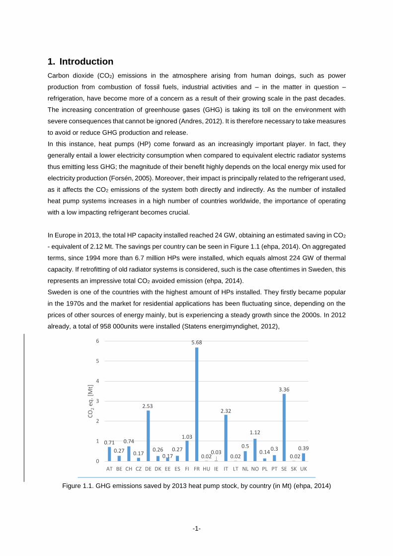
In Europe in 2013, the total HP capacity installed reached 24 GW, obtaining an estimated saving in CO2

- equivalent of 2.12 Mt. The savings per country can be seen in Figure 1.1 (ehpa, 2014). On aggregated

terms, since 1994 more than 6.7 million HPs were installed, which equals almost 224 GW of thermal

capacity. If retrofitting of old radiator systems is considered, such is the case oftentimes in Sweden, this

represents an impressive total CO2 avoided emission (ehpa, 2014).

Sweden is one of the countries with the highest amount of HPs installed. They firstly became popular

in the 1970s and the market for residential applications has been fluctuating since, depending on the

prices of other sources of energy mainly, but is experiencing a steady growth since the 2000s. In 2012

already, a total of 958 000units were installed (Statens energimyndighet, 2012),

Figure 1.1. GHG emissions saved by 2013 heat pump stock, by country (in Mt) (ehpa, 2014)

0.71

0.27

0.74

0.17

2.53

0.260.17

0.27

1.03

5.68

0.020.03

2.32

0.02

0.5

1.12

0.140.3

3.36

0.02

0.39

0

1

2

3

4

5

6

AT BE CH CZ DE DK EE ES FI FR HU IE IT LT NL NO PL PT SE SK UK

CO

2eq

. [M

t]

-2-

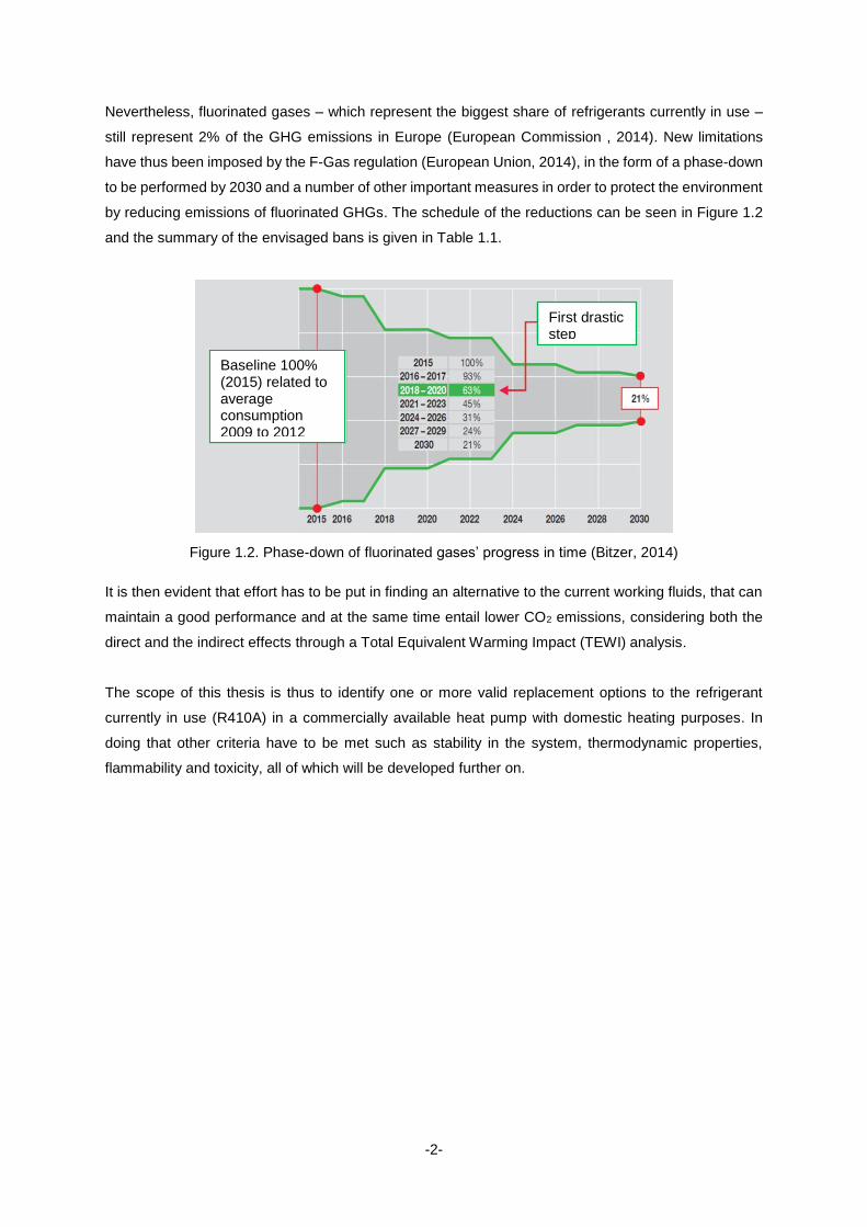
Nevertheless, fluorinated gases – which represent the biggest share of refrigerants currently in use –

still represent 2% of the GHG emissions in Europe (European Commission , 2014). New limitations

have thus been imposed by the F-Gas regulation (European Union, 2014), in the form of a phase-down

to be performed by 2030 and a number of other important measures in order to protect the environment

by reducing emissions of fluorinated GHGs. The schedule of the reductions can be seen in Figure 1.2

and the summary of the envisaged bans is given in Table 1.1.

Figure 1.2. Phase-down of fluorinated gases’ progress in time (Bitzer, 2014)

It is then evident that effort has to be put in finding an alternative to the current working fluids, that can

maintain a good performance and at the same time entail lower CO2 emissions, considering both the

direct and the indirect effects through a Total Equivalent Warming Impact (TEWI) analysis.

The scope of this thesis is thus to identify one or more valid replacement options to the refrigerant

currently in use (R410A) in a commercially available heat pump with domestic heating purposes. In

doing that other criteria have to be met such as stability in the system, thermodynamic properties,

flammability and toxicity, all of which will be developed further on.

Baseline 100% (2015) related to average consumption 2009 to 2012

First drastic step

-3-

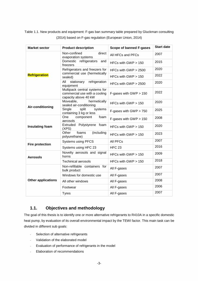
Table 1.1. New products and equipment: F-gas ban summary table prepared by Gluckman consulting

(2014) based on F-gas regulation (European Union, 2014)

Market sector Product description Scope of banned F-gases Start date

Refrigeration

Non-confined direct evaporation systems

All HFCs and PFCs 2007

Domestic refrigerators and freezers

HFCs with GWP > 150 2015

Refrigerators and freezers for commercial use (hermetically sealed)



All stationary refrigeration equipment


Multipack central systems for commercial use with a cooling capacity above 40 kW

F-gases with GWP > 150 2022

Air-conditioning

Moveable, hermetically sealed air-conditioning


Single split systems containing 3 kg or less


Insulating foam

One component foam aerosols


Extruded Polystyrene foam (XPS)


Other foams (including polyurethane)


Fire protection Systems using PFCS All PFCs 2007

Systems using HFC 23 HFC 23 2016

Aerosols

Novelty aerosols and signal horns


Techinical aerosols HFCs with GWP > 150 2018

Other applications

Non-refillable containers for bulk product

All F-gases 2007

Windows for domestic use All F-gases 2007

All other windows All F-gases 2008

Footwear All F-gases 2006

Tyres All F-gases 2007

1.1. Objectives and methodology

The goal of this thesis is to identify one or more alternative refrigerants to R410A in a specific domestic

heat pump, by evaluation of its overall environmental impact by the TEWI factor. This main task can be

divided in different sub goals:

- Selection of alternative refrigerants

- Validation of the elaborated model

- Evaluation of performance of refrigerants in the model

- Elaboration of recommendations

-4-

In order to accomplish the above-mentioned objectives, the work has mainly consisted of two phases.

First of all, a review of the state-of-the-art and of the latest research on the fourth generation refrigerants

has been performed and used as a base for the selection of a shortlist of possible alternatives to R410A.

The choice has been made following safety (no toxicity), environmental (no ODP and GWP lower than

R410A), and thermodynamic (suitable pressure and temperature characteristics) criteria.

Secondly, a model has been created on EES reproducing the functioning of the studied HP, and

validated against available experimental data and a second model created on IMST-ART.

The refrigerants have then been tested in such model, and results of environmental performance

compared with the baseline R410A.

1.2. Limitations of the model

The main limitations of this work lie in the applicability of the model and consist of:

- Compressor efficiency correlations unavailable for R32 and R1234ze(E), hence assumed.

- Compressor efficiency correlations unavailable for R450A and R513A.

- UA correlations for the heat exchangers obtained from regression analysis, thus limited to the

considered thermodynamic conditions and refrigerant

- Inlet brine temperature fixed at 0°C according to the Standard BS EN 14825:2012

The validity of the results can thus only be assured in the window of conditions considered in the

creation of the model.

1.3. Thesis’ structure

In chapter 2, an overview of the refrigerants’ main characteristics is given. It is followed by a summary

of the available literature on the most relevant possible alternatives to R410A. Finally, the selection of

the short-list of fluids to be analysed in the model is performed and motivated.

In chapter 3 the model utilised for the analysis of the performance is described, along with the

explanation of the calculations methods for the SCOP and TEWI factors.

Chapter 4 includes all the relevant results and the comparison between the contemplated options.

In chapter 5 the conclusion is given, and the necessary future work described.

-5-

2. Refrigerants

An overview of the different refrigerants’ categories will be given hereby, along with an outline of their

historical evolution. The main characteristics involved in the choice of alternatives will be developed,

and a summary of relevant studies performed on the most relevant options for the scope of this work

will be performed. Lastly, the shortlist of options to be further analysed will be illustrated.

2.1. Introductory concepts

The composition of a refrigerant, and thus some of its properties can be deduced by its name. The

structure is Raxyz, where R simply stands for Refrigerant, and, according to the ASHRAE Standard 34

(ANSI/ASHRAE, 2013):

x represents the number of Carbon atoms in the molecule, reduced by 1

When the number is zero it is omitted from the name.

y represents the number of hydrogen atoms, increased by 1

z is the number of fluorine atoms

a is the number of unsaturated carbon bonds. It is omitted when there are no double bonds.

It is to be noted that x=4 represents zeotropic mixtures (mixtures that experience a temperature glide

during phase changes), x=5 azeotropic mixtures (mixtures that behave as a pure substance), x=6

organic compounds and x=7 inorganic compounds. The concept of zeotropic behaviour will be

explained in section 2.2.1.

Although the vapour compression cycle was patented in the 19th century already (Balmer, 2011), the

research of optimal refrigerants, thermodynamically, economically and environmentally performing is

always ongoing. Throughout the history of the heat pump/refrigerating machine technology, different

groups of refrigerants have been used according to the current requirements and needs, as can be

seen in Figure 2.1.

-6-

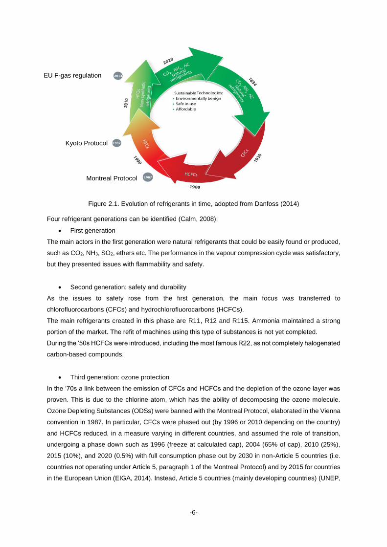
Figure 2.1. Evolution of refrigerants in time, adopted from Danfoss (2014)

Four refrigerant generations can be identified (Calm, 2008):

First generation

The main actors in the first generation were natural refrigerants that could be easily found or produced,

such as CO2, NH3, SO2, ethers etc. The performance in the vapour compression cycle was satisfactory,

but they presented issues with flammability and safety.

Second generation: safety and durability

As the issues to safety rose from the first generation, the main focus was transferred to

chlorofluorocarbons (CFCs) and hydrochlorofluorocarbons (HCFCs).

The main refrigerants created in this phase are R11, R12 and R115. Ammonia maintained a strong

portion of the market. The refit of machines using this type of substances is not yet completed.

During the ‘50s HCFCs were introduced, including the most famous R22, as not completely halogenated

carbon-based compounds.

Third generation: ozone protection

In the ‘70s a link between the emission of CFCs and HCFCs and the depletion of the ozone layer was

proven. This is due to the chlorine atom, which has the ability of decomposing the ozone molecule.

Ozone Depleting Substances (ODSs) were banned with the Montreal Protocol, elaborated in the Vienna

convention in 1987. In particular, CFCs were phased out (by 1996 or 2010 depending on the country)

and HCFCs reduced, in a measure varying in different countries, and assumed the role of transition,

undergoing a phase down such as 1996 (freeze at calculated cap), 2004 (65% of cap), 2010 (25%),

2015 (10%), and 2020 (0.5%) with full consumption phase out by 2030 in non-Article 5 countries (i.e.

countries not operating under Article 5, paragraph 1 of the Montreal Protocol) and by 2015 for countries

in the European Union (EIGA, 2014). Instead, Article 5 countries (mainly developing countries) (UNEP,

EU F-gas regulation

Kyoto Protocol

Montreal Protocol

-7-

2011) began with a freeze in 2013, followed by declining limits starting in 2015 (90%), 2020 (65%),

2025 (32.5%), and 2030 (2.5%), phase out in 2040.

Hydrofluorocarbons (HFCs) were developed as a replacement, having an ODP=0. Specifically, R134a

was created as a substitute of R12, entailing the possibility of keeping the same machine, provided

proper cleaning and oil changing. The interest in natural refrigerants was also reborn, still in a limited

measure.

Fourth generation: global warming avoidance

As the concern for the global warming phenomenon increased, a great responsibility was proven to

belong to the usage of fluorocarbons (FCs). New restrictions were established following the Kyoto

protocol, and the “Regulation of the European Parliament and of the Council on fluorinated gases and

repealing Regulation (EC) No 842/2006”or shortly, F-Gas regulation, was introduced. A first version

appeared in 2006, followed by a newer and somewhat stricter one applied since January 2015. Its main

aspects will be treated in section 2.2.5. Moreover, the “Directive 2006/40/ EC of the European

Parliament and of the Council relating to emissions from air-conditioning systems in motor vehicles and

amending Council Directive 70/156/EEC” (MAC regulation) regulates the use of fluorinated gases in

mobile air-conditioning systems (MACs) and requires a refrigerant with GWP ≤ 150 in new models of

cars after 2013.

It is important to understand that merely substituting an old refrigerant with a lower GWP may not be

enough. In fact, if the low GWP substance does not yield an optimum performance in the system it can

lead to an increase consumption of energy, and thus a greater indirect emission. A trade-off between

GWP and performance has therefore to be considered.

2.2. Characterisation of refrigerants

When evaluating a refrigerant a number of aspects has to be kept into consideration. In fact, in order to

be fit to operate in a heat pump, the fluid, pure or mixture, has to adhere to certain requirements that

can be divided in different categories, namely thermodynamic properties, chemical properties, safety

and environment issues. These groups will be treated in the following, and will be used as a starting

point for the selection process developed further in the report.

2.2.1. Thermodynamic characteristics

The influence of the refrigerant is particularly important on the condensation and evaporation processes,

as it defines the working pressures once that the temperatures are defined by the application.

Consequently it influences the design of the compressor and the expansion valve, as well as heat

exchange area in accordance to the required heat flux for the application.

In the case of a pure substance, to a certain saturated vapour pressure corresponds a particular

temperature as seen in Figure 2.2.

-8-

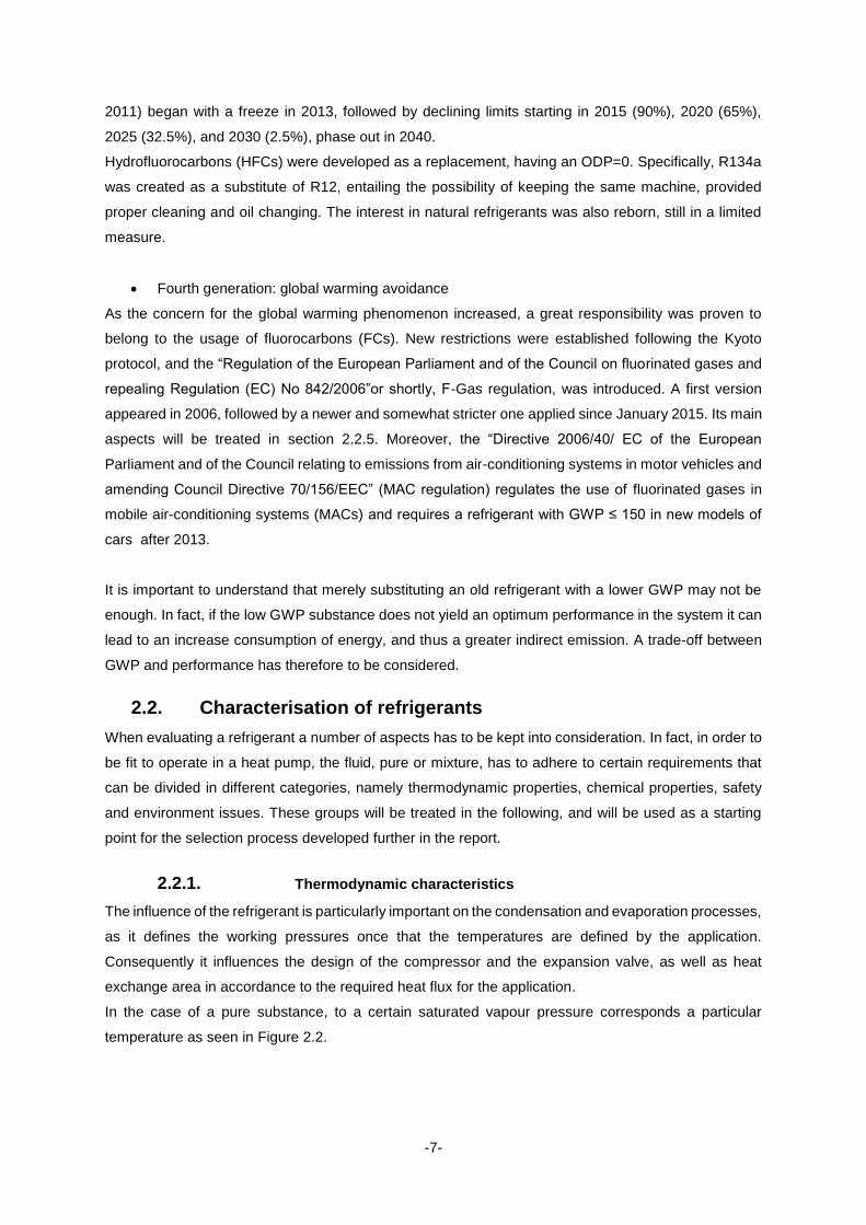
Figure 2.2. Saturated vapour pressure vs. temperature

Furthermore, the shape of the property diagram of a refrigerant influences the COP as it affects the

values of enthalpy at the saturation points (Ekroth, 2011).

As far as thermal characteristics are concerned, low vapour heat capacity, low viscosity and high

thermal conductivity should be maintained. The critical and boiling point temperatures must be chosen

relatively to the application. Additionally, it would be preferable to work with a refrigerant having a small

specific heat compared to the latent heat of vaporisation, in order to achieve smaller losses in the

expansion valve (Rothlin, 2011).

Another aspect of great importance to treat when considering refrigerants is the mixtures. Their

development and study is becoming increasingly important, as mixing different substances allows the

creation of working mediums with more suitable properties and that can also result in the increase of

the COP of the system.

According to their behaviour during evaporation and condensation, the mixtures can be classified as

azeotropic, near azeotropic, or zeotropic, the differences residing in if – and in what measure – a

temperature glide exists. In fact, when a pure refrigerant undergoes evaporation or condensation, it will

maintain a constant temperature as long as the pressure is kept constant. In general, an increased

pressure results in an increased saturated vapour pressure. Instead, in the case of a mixture of two or

more components, the above mentioned processes will occur with temperature varying with the liquid-

vapour composition.

Azeotropic mixtures

In this case the glide effect is not present: the mixture acts as a single substance, thus maintains a

constant boiling point, usually lower than either of the constituents. Most of these blends are binary and

are most commonly used in low temperature refrigeration applications.

0.1

1.0

10.0

100.0

-50 -40 -30 -20 -10 0 10 20 30 40 50 60 70 80 90 100

Pre

ssu

re [

ba

r]

Temperature [˚C]

R410A

R134a

R513A

R450A

R32

R1234yf

R1234ze

R152a

Isobutane

Propane

Propylene

-9-

Near azeotropic mixtures

It applies when the temperature glide is very small, of the order of 0.2 – 0.6 ºC. It is to be noted that the

properties and composition of this kind of mixture can change if leakage occurs. They share most of

the properties of the azeotropic mixtures, yet giving a broader range of possibilities (Mohanraj, 2011).

R410A is an example of near-azeotropic mixture in residential HP application. The new mixtures R450A

and R513A also belong to this category.

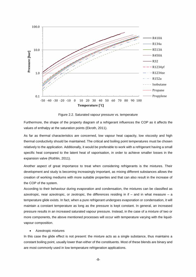
Zeotropic mixtures

During the state changes the mixture will no longer behave as a single substance. The temperature

glide needs to be considered in this case. Furthermore, the evaporation and condensation processes

cannot be considered as isothermal anymore. In the first case the most volatile component – the one

with the highest vapour pressure at a given temperature – will start the evaporation first; in the latter the

opposite is true. Practically, this implies an increasing saturation temperature along the evaporator and

a decreasing one along the condenser, as seen Figure 2.3. Moreover, the composition of the liquid will

change throughout the vaporisation.

In this case a distinction must be made between “starting” and “stopping” evaporation temperature, and

thus the bubble point temperature and the dew point temperature are defined.

This kind of mixture usually results from the addition of a third component, which can be needed to

improve the characteristics of the substance. For example, such an addition could result in lower

flammability, better oil miscibility etc. On the other hand, an enhanced leakage, due to the most volatile

component is present (SWEP International AB, 2012).

Figure 2.3. Condenser (right) and evaporator (left) temperature profiles (SWEP International AB,

2012)

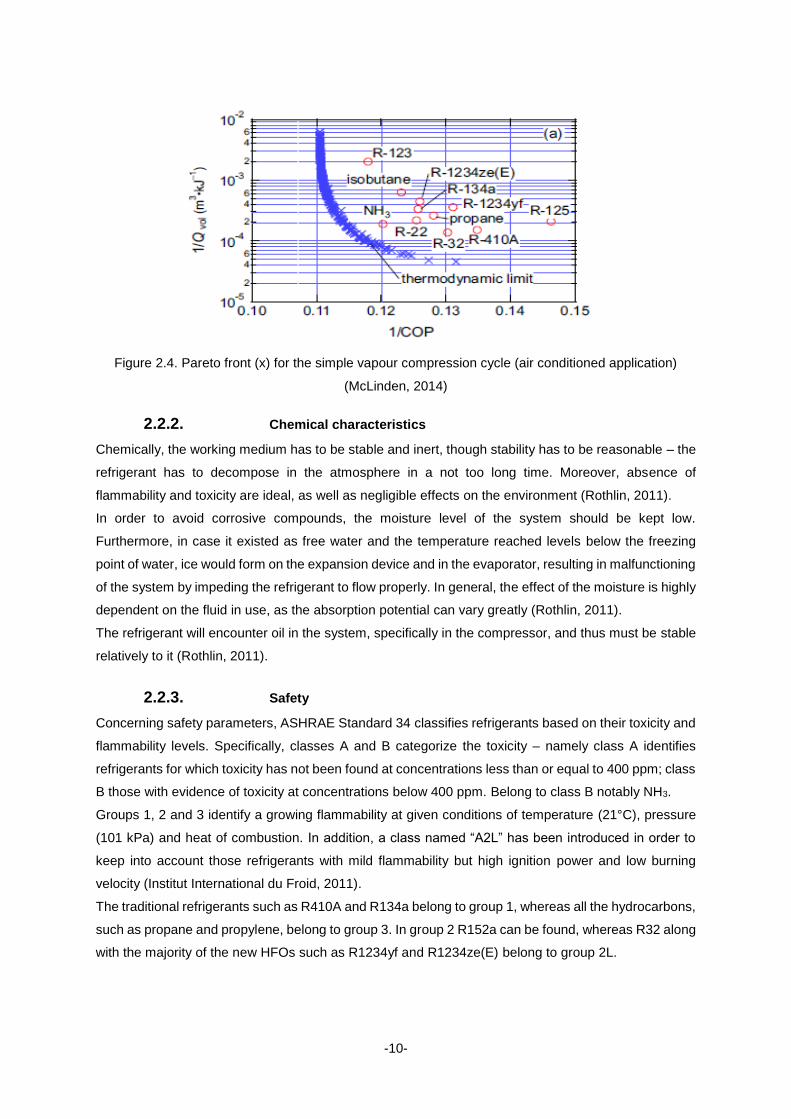
When selecti ng a refrigerant a number of thermodynamic requirements exist, and can hardly be

satisfied without any compromise. This phenomenon can be exemplified with a Pareto analysis, e.g. as

in Figure 2.4. It represents the thermodynamic limit to the performance of a specific cycle, given the

evaporation and condensation temperatures, and thus the application. It illustrates the trade-off

between the volumetric capacity and the COP and states that it is not possible to achieve both a high

COP and high capacity. The better the refrigerant, the closer it lies to the Pareto front (McLinden, 2014).

Brine

Length [m] Length [m]

-10-

Figure 2.4. Pareto front (x) for the simple vapour compression cycle (air conditioned application)

(McLinden, 2014)

2.2.2. Chemical characteristics

Chemically, the working medium has to be stable and inert, though stability has to be reasonable – the

refrigerant has to decompose in the atmosphere in a not too long time. Moreover, absence of

flammability and toxicity are ideal, as well as negligible effects on the environment (Rothlin, 2011).

In order to avoid corrosive compounds, the moisture level of the system should be kept low.

Furthermore, in case it existed as free water and the temperature reached levels below the freezing

point of water, ice would form on the expansion device and in the evaporator, resulting in malfunctioning

of the system by impeding the refrigerant to flow properly. In general, the effect of the moisture is highly

dependent on the fluid in use, as the absorption potential can vary greatly (Rothlin, 2011).

The refrigerant will encounter oil in the system, specifically in the compressor, and thus must be stable

relatively to it (Rothlin, 2011).

2.2.3. Safety

Concerning safety parameters, ASHRAE Standard 34 classifies refrigerants based on their toxicity and

flammability levels. Specifically, classes A and B categorize the toxicity – namely class A identifies

refrigerants for which toxicity has not been found at concentrations less than or equal to 400 ppm; class

B those with evidence of toxicity at concentrations below 400 ppm. Belong to class B notably NH3.

Groups 1, 2 and 3 identify a growing flammability at given conditions of temperature (21°C), pressure

(101 kPa) and heat of combustion. In addition, a class named “A2L” has been introduced in order to

keep into account those refrigerants with mild flammability but high ignition power and low burning

velocity (Institut International du Froid, 2011).

The traditional refrigerants such as R410A and R134a belong to group 1, whereas all the hydrocarbons,

such as propane and propylene, belong to group 3. In group 2 R152a can be found, whereas R32 along

with the majority of the new HFOs such as R1234yf and R1234ze(E) belong to group 2L.

-11-

2.2.4. Environmental issues

Nowadays, for a refrigerant to be considered benign to the environment, it has to entail no harm to the

ozone, and low contribution to the greenhouse effect. Two indicators need thus consideration.

Firstly, the Ozone Depletion Potential (ODP) is used to evaluate the impact of the substance on the

ozone layer. In fact, elements such as Chlorine and Bromine, when dispersed in the atmosphere, result

in the breakdown of the ozone molecule O3, in a sequence of loop reactions that lead to the destruction

of many ozone molecules by a single Cl atom. The evaluation of the ODP is made by referring the effect

of a substance to the one of R11, considered having ODP=1 (IPCC, 2005).

Secondly, the greenhouse effect contribution is assessed by the Global Warming Potential (GWP). The

evaluation is made by comparing the ability of absorbing heat by the gas, per unit of weight, relatively

to CO2, which is considered to have GWP=1. The decay rate of the gas is also taken into account, i.e.

the quantity removed from the atmosphere in a given number of years. It is easily understood that the

shorter the lifetime in the atmosphere of the substance, the better (Global Greenhouse Warming, 2015).

For a complete evaluation of the environmental impact of the refrigerant, though, these two parameters

are not sufficient. A more thorough analysis can be performed with a TEWI study. The TEWI indicator

comprehends the total impact of the substance throughout the lifetime of refrigeration system, and

considers not only the direct impact – due to leakages of the working fluid during the operation of the

machine and during its dismissal – but also the indirect one, that is mainly due to the energy used for

the functioning of the system, and is thus variable in accordance to the location and the energy sources

used.

The calculation of this value, expressed in kg of CO2 - equivalent emissions of GHG, can be performed

as in equation (2.1).

𝑇𝐸𝑊𝐼 = (𝐺𝑊𝑃 ∗ 𝐿𝑎𝑛𝑛𝑢𝑎𝑙 ∗ 𝑁) + 𝐺𝑊𝑃 ∗ 𝑚 ∗ (1 − 𝛼𝑟𝑒𝑐𝑜𝑣𝑒𝑟𝑦) + (𝑁 ∗ 𝐸𝑎𝑛𝑛𝑢𝑎𝑙 ∗ 𝛽)

(2.1)

where GWP is the global warming potential of refrigerant (kgCO2/kgref), Lannual the leakage rate in the

system (kgref/year), m is the refrigerant charge (kgref), N the lifetime of the system (years), 𝛼𝑟𝑒𝑐𝑜𝑣𝑒𝑟𝑦 the

recycling factor, Eannual the energy consumption per year (kWh/year), β the CO2 emission factor

(kgCO2/kWh) (Mohanraj, 2011) (AIRAH, 2012).

2.2.5. Policies

In order to reduce the environmental impact of human activities, a number of protocols and regulations

have been prepared along the years. Within the most famous are Kyoto protocol, Montreal protocol and

lastly, aiming at protecting the environment by reducing emissions of fluorinated GHGs, and thus

motivation behind this work, the F-gas regulation. A first version was adopted in 2006, followed by a

second version to replace it, applied from the 1st January 2015.

The main goal is to reduce the contribution of the refrigeration industry to the global warming, by cutting

the consumption of fluorinated gases (F-gases) by 79% by 2030, with start at 2009-2012 average level

Direct: leakage Indirect: operation

-12-

(European Union, 2014). The expected outcome is a reduction of 1.5 Gt of CO2-equivalent by 2030 and

5 Gt by 2050 from 2009-2012 average level. Currently, the F-gases represent 2% of the GHG emissions

in Europe, and the growth has been of almost 60% since 1990. (European Commission , 2014).

Additionally, the regulation imposes the phase down of refrigerants with GWP over the allowed limits

and the restriction on the marketing and use of some of these products; it aims also at improving the

prevention of leaks that contribute to the direct impact of the refrigeration and air conditioning units.

The main points included in the new regulation are (Bitzer, 2014):

Phase-down of the fluorinated gases currently in use. The percentage requirement is calculated

on the CO2 equivalent basis (Figure 1.2). It is to be noted that the phase down only applies to

HFCs and not to other fluorinated gases such as FCs or sulphur hexafluoride (SF6).

Introduction of a quota system. For each producer or importer, quotas indicating maximum

quantities for every year from 2015 will be specified. A baseline value is calculated on the 2009-

2012 average volume placed on the market by each producer/importer, and the maximum

quantity are calculated as percentages on this reference value (table in Figure 1.2). The quota

received corresponds to 89% of the reference value multiplied by the percentage indicated for

every year. The remaining 11% is allocated to new undertakings (AREA, 2014).

The limitations will apply to products manufactured in countries that don’t belong to the

European Union as well, that will only be importable if subjected to the quota system.

A maximum GWP is defined for some applications, thus limiting from 2015 already the usage

of some refrigerants in particular segments, such as domestic refrigerators and freezers Table

1.1.

Leakage prevention and treatment. A schedule of mandatory checks is prepared in accordance

with the application and size of the technology used, for all cases where a refrigerant charge

higher than 5 tons of CO2 equivalent.

The application of such a quantitative limit implies the long-term usage of new refrigerants with GWP <

500 at the most, with repercussions on systems not currently directly affected by the bans, as the

requirements for refrigeration are expected to increase (Bitzer, 2014).

Worldwide, other measures have been taken. In particular, in North America, the Significant New

Alternatives Policy (SNAP) has been introduced as an EPA’s (Environmental Protection Agency)

program to evaluate and regulate substitutes for class I (ODP ≥ 0.2) and class II (ODP < 0.2) ozone

depleting substances under the Clean Air Act indications and moved in 2014 towards the

implementation of new rules, making certain high GWP refrigerants unacceptable in various end-uses

(Environmental Protection Agency, 2015).

-13-

2.3. State of the art of the fourth generation of refrigerants

The new restrictions imposed by the F-gas regulation pushed the research of new refrigerants or blends

that could be efficient replacements to high GWP refrigerants, with minimal modifications to current

system technologies, at the lowest possible cost. Concerning the environmental aspect, it is

fundamental to consider both the direct and indirect effect of the substances; e.g. by the means of the

TEWI calculation. This way, wrong conclusions can be avoided; in fact, a refrigerant with low GWP

could actually have a higher indirect impact because of the poorer performance in the system.

Generally, the literature available is rather limited, as some of the upcoming options are new substances

and mixtures and still lack vast experimentation.

McLinden et al. (2014) conducted studies on over 56 000 molecules, with 15 or fewer atoms and

comprising only the elements C, H, F, Cl, Br, O, N, and/or S that were successively screened by their

ODP, GWP and various properties, reducing the number of candidates to 1200. When applying further

criteria, such as having an appropriate critical temperature (between 300 and 400 K for almost all of the

common refrigerating applications), 62 candidates were left. The most promising ones for residential

heat pump systems, divided in categories, will be described in this section. A further elimination process

will then be performed and motivated, leading to the shortlist of options presented in section 2.4.

2.3.1. HFCs

The most relevant for the considered application belonging to this category are R410A, R134a, R152a

and R32. The GWP is still not optimal, and thus they should be regarded as medium term solutions.

HFC/HC blends

The addition of a HC element to the HFC mixture improves the solubility with the lubricant, in extreme

cases allowing the use of conventional oils, thus removing the need for retrofitting. Furthermore, the

flammability of the HC blends can be reduced by the mixing of a HFC.

R134a

Due to its high GWP (1300), it has been limited from MAC applications and banned in new vehicles’

models from 2013 with the MAC regulation, and will be phased down in other applications. In fact, it will

be allowed until 2022 in commercial hermetically sealed equipment (GWP<2500). In 2022 the limit to

GWP will be set to 150, thus making R134a unacceptable.

R152a

It has a critical temperature lower than 400 K, and presents a flammability level of A2. Usually used as

a component in a mixture and can substitute, in a transitional manner, R134a. (McLinden, 2014).

The literature available regarding HP applications is limited, proving that the research on this refrigerant

is still at an early stage. Ho-Saeng Leea et al. (2012) performed a study in a water source heat pump

system on a R152a/R32 mixture, with varying percentual composition of R32. It was found that the

tested system required a compressor power up to 13.7% lower when compared to an equivalent R22

system, along with an increased COP (up to 15.8%); the refrigerant charge diminishes of up to 27%.

On the other hand, the compressor discharge temperature is increased up to 15.4 °C.

-14-

R32

Its flammability is classified at A2L, and GWP is 675. Products using R32 are already in the market,

such as the Daikin air-to-air heat pump (Daikin Global , 2014).

In an analysis by Barve et al. (2010), when compared to an R410A based equivalent HP and for an

outdoor temperature varying between -8 to 46°C, the R32 system was found to have comparable

cooling and heating capacities and similar COP. Though, an increase in the discharge pressure and

temperature was measured which can be a concern to the compressor lifetime. An observable positive

aspect is the decrease in the refrigerant charge that could lead to the usage of a smaller compressor.

Hakkaki-Fard et al. (2014) conducted a study with the goal of finding a refrigerant (pure or mixture) that

could have a good performance in domestic applications (small/medium heat pumps), in comparison to

an equivalent R410A, also involving the least number of modifications possible. Within a selection of

15 options, the mixture that emerged as best is R32/CO2 (80/20). Combining the two elements has in

fact the double advantage of reducing the flammability of R32 and mitigating the high pressure of CO2.

The obtained blend, furthermore, presents a higher heating capacity than R410A – that can be

increased even more by augmenting the size of the heat exchangers – in spite of a slightly smaller

COP. The GWP is reduced as approximately 25% of the baseline.

2.3.2. Natural Refrigerants

They present a low direct impact, with ODP=0 and low (or zero) GWP, accompanied with high efficiency

that results in low indirect impact as well.

Ammonia NH3 (R717)

It is one of the oldest refrigerants known, and has zero GWP and ODP. It presents a low boiling point

and is acknowledged as one of the most efficient refrigerants. The most common applications are

industrial refrigeration, transport refrigeration, industrial/commercial air conditioning DX chillers and

industrial/commercial centrifugal compressors. It is mainly being considered as a substitute for R22 and

R134a (Linde, 2015). The main limits to its usage in other application rather than big industrial systems

are its flammability and mild toxicity. By the means of a screw compressor, which results in a lower

discharge temperature, and of plate type heat exchangers, that involve a smaller quantity of refrigerant,

it is now possible to build relatively safe low charge ammonia systems. Though, its toxicity still prevents

the diffusion in many locations, mainly where a warm climate is present (Bathkar, 2013). Evaluation of

mixtures having ammonia as a component exists in the literature, and the general outcome is a lower

discharge temperature, thus resulting in a longer life of the compressor (Mohanraj, 2011).

CO2 (R744)

As a natural refrigerant, as was the case for NH3, CO2 presents zero ODP and GWP=1. Moreover, it is

a non-toxic and non-flammable substance. The most common applications are commercial, industrial

and transport refrigeration, industrial/commercial air conditioning DX chillers, industrial/commercial

centrifugal compressors and mobile air conditioning (Linde, 2015).

A drawback of its implementation is the necessity of significant modifications to the system, since CO2

operates with much higher pressure than HFCs and with a lower critical temperature. On the other

hand, it offers higher values of density, latent heat, specific heat, thermal conductivity and volumetric

-15-

cooling capacity. Because of the above-mentioned low critical temperature, R744 can be run in a trans-

critical cycle. This means that the working medium would evaporate in the subcritical region and

successively reject heat in a gas cooler instead of a condenser, at temperatures above the critical point

(Bathkar, 2013).

2.3.3. HCs

An advantage with this type of refrigerants is their miscibility with synthetic lubricants and mineral oil.

These fluids therefore do not have to be changed when switching from HCFC or HFC mixtures to HC

ones. Besides, their short atmospheric life results in a very low GWP and they represent the best choice

when considering their cost. On the other hand, they present problems because of their flammability.

The two main HCs used as refrigerants are isobutane (refrigerators) and propane (small commercial

appliances and residential heat pumps). Many examples of blends involving HCs, with different

components and variable relative percentages in mass, exist in the literature. The general conclusion

seems to be a lower energy consumption, compared to both equivalent R134a and R22 systems.

In conclusion, HC mixtures are a good alternative in small applications such as domestic refrigeration,

small capacity refrigeration and heat pump units and MAC systems (Mohanraj, 2011) (Bathkar, 2013).

R290 (propane)

It has environmental and thermodynamic outstanding characteristics but, as HC, has high flammability

and thus cannot be implemented in existing FC systems. Moreover, because of the safety issues it is

only applicable in industrial/commercial refrigeration systems and air conditioning, as well as domestic

air conditioning, provided proper refitting. Restrictions to the placement of the system and to the

refrigerant charge are imposed by the Standard EN378 (EN 378, 2008). Despite the flammability

concerns, research is active and products are being brought to the market from companies such as Ait-

Deutschland (Maul, 2013).

In order to lessen the flammability, mixtures can be used. Ki-Jung Park et al. (2009) investigated for

example a mixture of R170/R290 (with varying relative composition) in a heat pump as a substitute for

R22, both in summer and winter conditions. The results showed an increase in the COP of up to 15.4%,

despite a decrease in the capacity (up to -7.5%). Other observed improvements of the system are the

decrease in the compressor discharge temperature and a reduction in the refrigerant charge.

Fan et al. (2013) investigated a R744/R290 mixture, finding an increased COP, along with an increased

volumetric heating capacity when compared to an equivalent R22 system. Though, it is observed that

the performance is efficient only when working with large heat-sink temperature rise.

R1270 (propylene)

Literature is very limited, and major studies still need to be performed. The environmental characteristics

are optimal, but propylene, as propane, implies an A3 flammability level and thus is not suitable for

retrofitting existing systems. It is most adapt to low – medium temperature applications. (Linde , 2015).

Propylene is an unsaturated molecule and therefore its stability is lower than that of propane. Therefore

the latter is often given priority to the former when selecting an environmentally friendly refrigerant.

-16-

2.3.4. HFOs

HFOs have been on the rise since the 2010s, as they present a very low GWP, along with zero ODP.

In fact, HFOs are derivatives of alkenes rather than alkanes and thus are unsaturated, i.e. they have a

double bond in the molecule, which results in a short atmospheric life. The main disadvantage is the

mild flammability of most HFOs, that can be a barrier to the implementation in small systems such as

domestic and commercial refrigeration/heat pump units (Bathkar, 2013). Besides, they currently entail

a much higher cost of manufacturing.

Between the possibilities offered by HFOs, the most promising solutions are represented by R1234yf,

R1234ze(E) and R1234ze(Z) and their mixtures; they aim primarily at substituting R134a and R114 in

domestic refrigeration and mobile air conditioning applications (R1234yf) and in commercial

refrigeration, industrial air conditioning and heat pumps and heat transfer applications (R1234ze(E),

R1234ze(Z)) (Linde, 2015).

The data found in the literature is limited and varies between different authors. The studies conducted

by Zhang et al. (2014) had a positive outcome; the heat transfer coefficient of R1234yf was in fact

estimated to be lower in the condenser and higher in the evaporator compared to an R134a equivalent

system. Moreover, it belongs to the class A2L.

Concerning high temperature heat pumps, a number of mixtures were tested and good results were

shown by the mixture M1A (R1234zf/HC-290, 60%/40% in the mass) such as higher COP and lower

discharge temperature, compared to an equivalent R114 system (Zhang, 2014).

A series of 54 experiments on R1234yf and R1234ze(E) were carried by Mota-Babiloni et al. (2014) as

drop-in replacements in R134a systems. In this case the average COP was reported to be lower that

the baseline one, as well as the cooling capacity. The performance can be improved with the usage of

an Internal Heat Exchanger (IHX), which affects in a bigger measure both HFOs’ systems than the

R134a one. It is to be noted that an R134a machine operates with a reciprocating compressor, whereas

screw or centrifugal would be more appropriate for R1234ze(E). Furthermore, the difference in

performance is reduced by increasing the condensation temperature (R1234yf) or increasing

evaporation temperature (R1234ze(E)).

To overcome some of the limitations imposed by HFOs, mixtures can be used. Within the most

interesting options are R450A and R513A.

Mota-Babiloni et al. (2014) investigated the performance of R450A (R1234ze(E)/R134a mixture, 58/42

in mass percentage) as a transitional replacement of R134a, having good performance, similar

operation conditions but though a GWP still quite high (601). The resulting blend is also non-flammable,

and near-azeotrope. The outcome is a higher COP, mainly due to a much lower compressor power

consumption, and lower discharge temperature, in spite of a lower cooling capacity. In this case the IHX

has a smaller influence in the way that it affects both systems in a similar way and thus doesn’t have

particular interest. R450A can be used satisfactorily in an R134a system, but a refit is advisable to

optimise its performance.

-17-

Concerning R513A, a mixture of R134a/R1234yf (44/56 in mass percentage), the available literature is

very limited. Similarly to R450A, it is non-flammable, and has a GWP of 631.

Schultz and Kujak (2013) performed drop-in tests of R513A in an R134a chiller, obtaining a comparable

capacity, but an efficiency reduction of 3-4%.

2.4. Selected refrigerants for further analysis

When selecting the refrigerants to elaborate a shortlist of R410A replacement options within the

described above, the criteria kept into consideration can be summarised as follows:

Low GWP, no ODP

Non-toxic

Chemical and thermal stability, inert

Suitable physical and thermodynamic properties:

– Critical point and boiling point temperatures appropriate for the application

– Low vapour heat capacity

– Low viscosity

– High thermal conductivity

Compatibility with materials, miscibility with lubricants

Other:

– High dielectric strength of vapour

– Low freezing point

– Easy leak detection

– Low cost

It is evident that a compromise must be sought, as no refrigerant currently available can satisfy all of

the characteristics ideally requested.

A low GWP is considered for a preliminary round of elimination, as the alternative refrigerant has to

have a GWP at least inferior to R410A (2088). This eliminates R134a.

As far as safety is concerned, toxic refrigerants (classified B by the ASHRAE 34) will not be considered

as options, whereas flammability will not be a deterring in this phase of the research. Hence, ammonia

will not be analysed further.

The main thermodynamic aspects to be kept into account can be summarised in Figure 2.5, applied to

the saturated vapour pressure curves, seen in Figure 2.2. The operational envelope identified in the

figure by the red square is built by combining pressure and temperature boundaries to the refrigerants.

-18-

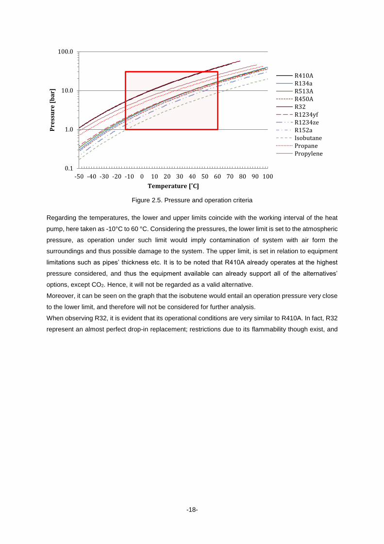
Figure 2.5. Pressure and operation criteria

Regarding the temperatures, the lower and upper limits coincide with the working interval of the heat

pump, here taken as -10°C to 60 °C. Considering the pressures, the lower limit is set to the atmospheric

pressure, as operation under such limit would imply contamination of system with air form the

surroundings and thus possible damage to the system. The upper limit, is set in relation to equipment

limitations such as pipes’ thickness etc. It is to be noted that R410A already operates at the highest

pressure considered, and thus the equipment available can already support all of the alternatives’

options, except CO2. Hence, it will not be regarded as a valid alternative.

Moreover, it can be seen on the graph that the isobutene would entail an operation pressure very close

to the lower limit, and therefore will not be considered for further analysis.

When observing R32, it is evident that its operational conditions are very similar to R410A. In fact, R32

represent an almost perfect drop-in replacement; restrictions due to its flammability though exist, and

0.1

1.0

10.0

100.0

-50 -40 -30 -20 -10 0 10 20 30 40 50 60 70 80 90 100

Pre

ssu

re [

ba

r]

Temperature [˚C]

R410AR134aR513AR450AR32R1234yfR1234zeR152aIsobutanePropanePropylene

-19-

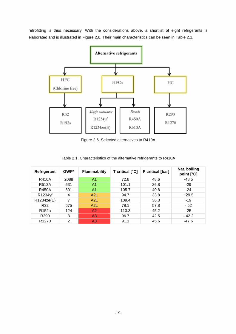
retrofitting is thus necessary. With the considerations above, a shortlist of eight refrigerants is

elaborated and is illustrated in Figure 2.6. Their main characteristics can be seen in Table 2.1.

Figure 2.6. Selected alternatives to R410A

Table 2.1. Characteristics of the alternative refrigerants to R410A

Refrigerant GWP* Flammability T critical [°C] P critical [bar] Nat. boiling

point [°C]

R410A 2088 A1 72.8 48.6 -48.5

R513A 631 A1 101.1 36.8 -29

R450A 601 A1 105.7 40.8 -24

R1234yf 4 A2L 94.7 33.8 −29.5

R1234ze(E) 7 A2L 109.4 36.3 -19

R32 675 A2L 78.1 57.8 - 52

R152a 124 A2 113.3 45.2 -25

R290 3 A3 96.7 42.5 - 42.2

R1270 2 A3 91.1 45.6 -47.6

-20-

-21-

3. Analysis of the developed model

The product considered in the scope of the testing is a commercial model available in the market as the

representative of domestic heat pump installed in a Swedish single family house, with 10 kW heating

capacity. The modelling of the said heat pump has been conducted in the EES software, an equation

solver tool able to solve systems of thousands of non-linear equations. Its major feature and main

reason for its choice is the fact that it contains all the thermodynamic properties of the major refrigerants

and comprises an extensive library of correlations.

In order to evaluate the indirect effect that has to be kept into account while calculating the TEWI, the

SCOP is obtained from the model.

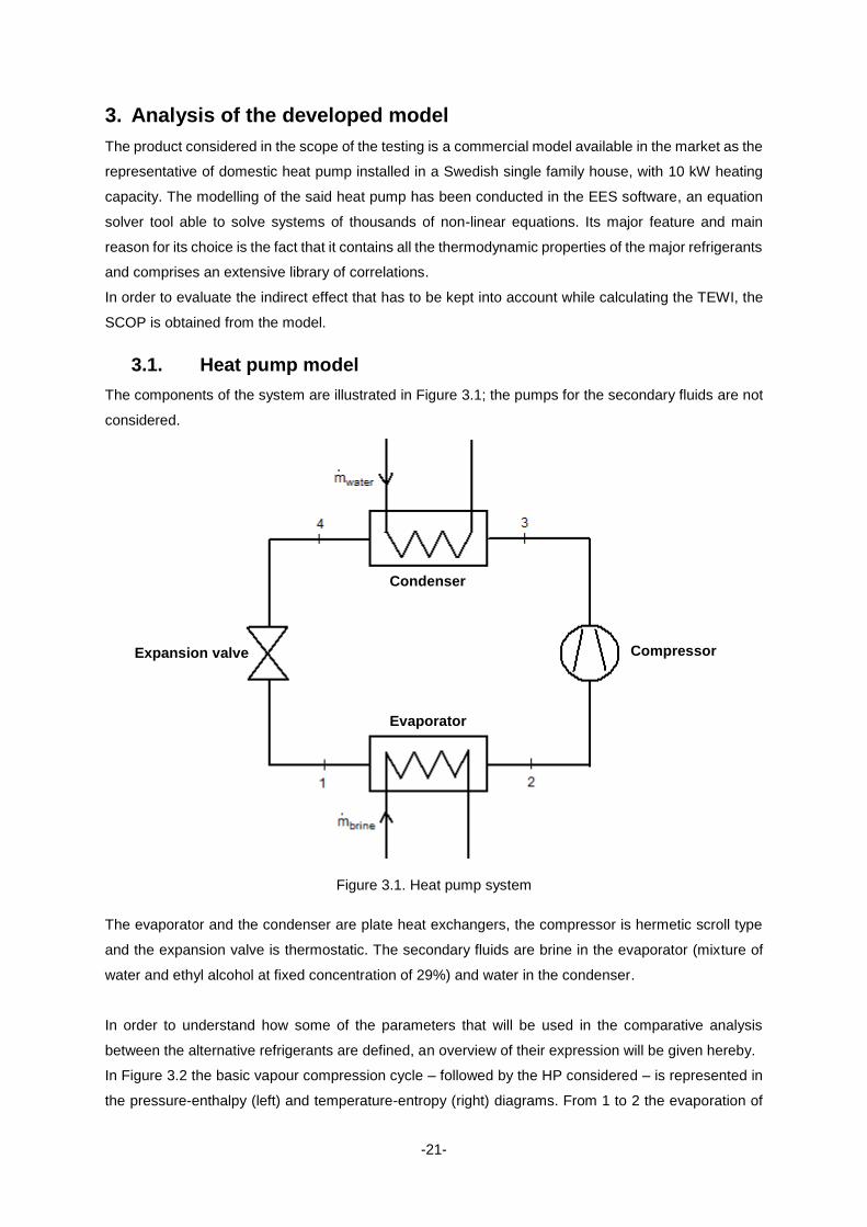
3.1. Heat pump model

The components of the system are illustrated in Figure 3.1; the pumps for the secondary fluids are not

considered.

Figure 3.1. Heat pump system

The evaporator and the condenser are plate heat exchangers, the compressor is hermetic scroll type

and the expansion valve is thermostatic. The secondary fluids are brine in the evaporator (mixture of

water and ethyl alcohol at fixed concentration of 29%) and water in the condenser.

In order to understand how some of the parameters that will be used in the comparative analysis

between the alternative refrigerants are defined, an overview of their expression will be given hereby.

In Figure 3.2 the basic vapour compression cycle – followed by the HP considered – is represented in

the pressure-enthalpy (left) and temperature-entropy (right) diagrams. From 1 to 2 the evaporation of

Expansion valve

Condenser

Compressor

Evaporator

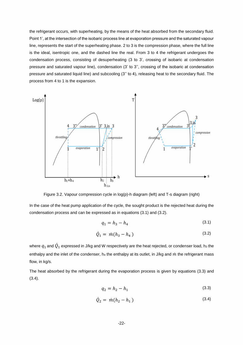
-22-

the refrigerant occurs, with superheating, by the means of the heat absorbed from the secondary fluid.

Point 1’, at the intersection of the isobaric process line at evaporation pressure and the saturated vapour

line, represents the start of the superheating phase. 2 to 3 is the compression phase, where the full line

is the ideal, isentropic one, and the dashed line the real. From 3 to 4 the refrigerant undergoes the

condensation process, consisting of desuperheating (3 to 3’, crossing of isobaric at condensation

pressure and saturated vapour line), condensation (3’ to 3’’, crossing of the isobaric at condensation

pressure and saturated liquid line) and subcooling (3’’ to 4), releasing heat to the secondary fluid. The

process from 4 to 1 is the expansion.

Figure 3.2. Vapour compression cycle in log(p)-h diagram (left) and T-s diagram (right)

In the case of the heat pump application of the cycle, the sought product is the rejected heat during the

condensation process and can be expressed as in equations (3.1) and (3.2).

𝑞1 = ℎ3 − ℎ4 (3.1)

�̇�1 = �̇�(ℎ3 − ℎ4 ) (3.2)

where 𝑞1 and �̇�1 expressed in J/kg and W respectively are the heat rejected, or condenser load, h3 the

enthalpy and the inlet of the condenser, h4 the enthalpy at its outlet, in J/kg and �̇� the refrigerant mass

flow, in kg/s.

The heat absorbed by the refrigerant during the evaporation process is given by equations (3.3) and

(3.4).

𝑞2 = ℎ2 − ℎ1 (3.3)

�̇�2 = �̇�(ℎ2 − ℎ1 ) (3.4)

-23-

where 𝑞2 and �̇�2 expressed in J/kg and W respectively are the heat absorbed, or evaporator load, h1

and h2 the enthalpies and the inlet and outlet of the evaporator respectively, in J/kg and �̇� the

refrigerant mass flow, in kg/s.

The required work, ideal and real, are given by equations (3.5) and (3.6).

𝑤𝑖𝑑 = ℎ3,𝑖𝑠 − ℎ2 (3.5)

𝑤 = ℎ3 − ℎ2 (3.6)

where 𝑤𝑖𝑑 and 𝑤 are expressed in J/kg.

In a real vapour compression system, the enthalpy at the exit of the compressor differs from the

isentropic one, as the losses in this component cannot be neglected.

The isentropic efficiency of the compressor can thus be defined according to (3.7).

ηis = h3,is − h2

h3 − h2

(3.7)

The performance of a refrigerating cycle is evaluated through the coefficient of performance (COP).

To represent the difference in the purpose of the heat pump and the refrigerating machine, two different

COP can be expressed. In the case of a heat pump, the desired product is the rejected heat and thus

the COP is given by (3.8); in the case of a refrigerating machine, the sought effect is the absorbed heat

and therefore the COP is given by (3.9).

𝐶𝑂𝑃1 = �̇�1/�̇� (3.8)

𝐶𝑂𝑃2 = �̇�2/�̇� (3.9)

where �̇�1 is the rejected heat during the condensation process, �̇�2 the absorbed heat during evaporation

and W is the required net work input, in kW.

The COP1 of the heat pump can also be thought of as a multiplier, representing the number of times

the used work is gained as heat at the higher temperature level.

The relationship between the two COPs, in the same machine – operating at the same conditions – can

be expressed as seen in (3.10).

𝐶𝑂𝑃1 = 𝐶𝑂𝑃2 + 1 (3.10)

3.1.1. Basic assumptions

A set of experimental data obtained from runs of the real heat pump were available and were used as

starting points for the creation of the model. Specifically, the runs were classified by inlet temperature

of brine in the evaporator (0, 5, -5 °C) and outlet temperature of water in the condenser (35, 45, 55 ºC),

creating a combination of nine runs. Superheat is set at 4.8 °C and subcooling at 4 °C.

Overall, the input data chosen are as seen in Table 3.1:

-24-

Table 3.1. Input data

Amount of superheat [ºC]

Amount of subcooling [ºC]

Inlet temperature of brine [ºC]

Outlet temperature of water [ºC]

Mass flow [kg/s]

Specific heat [kJ/kg-°C]

3.1.2. Evaporator

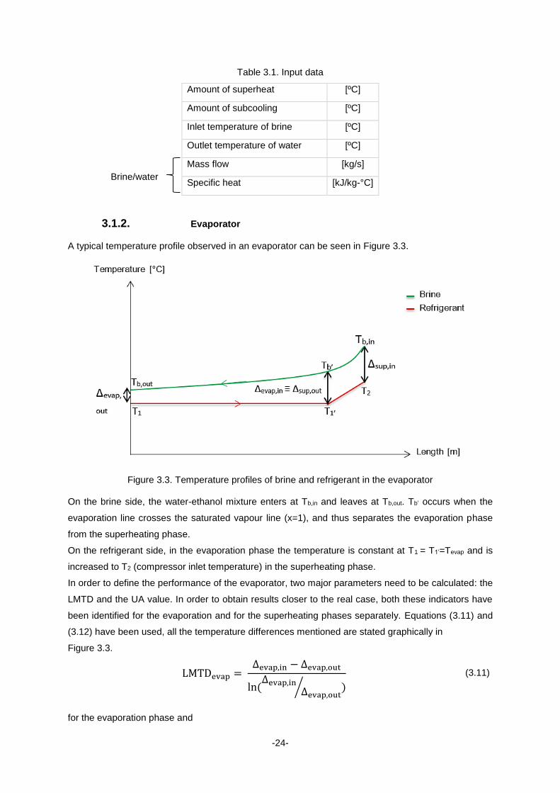
A typical temperature profile observed in an evaporator can be seen in Figure 3.3.

Figure 3.3. Temperature profiles of brine and refrigerant in the evaporator

On the brine side, the water-ethanol mixture enters at Tb,in and leaves at Tb,out. Tb’ occurs when the

evaporation line crosses the saturated vapour line (x=1), and thus separates the evaporation phase

from the superheating phase.

On the refrigerant side, in the evaporation phase the temperature is constant at T1 = T1’=Tevap and is

increased to T2 (compressor inlet temperature) in the superheating phase.

In order to define the performance of the evaporator, two major parameters need to be calculated: the

LMTD and the UA value. In order to obtain results closer to the real case, both these indicators have

been identified for the evaporation and for the superheating phases separately. Equations (3.11) and

(3.12) have been used, all the temperature differences mentioned are stated graphically in

Figure 3.3.

LMTDevap = Δevap,in − Δevap,out

ln(Δevap,in

Δevap,out⁄ )

(3.11)

for the evaporation phase and

Brine/water

-25-

LMTDSH = ΔSH,in − ΔSH,out

ln(ΔSH,in

ΔSH,out⁄ )

(3.12)

for the superheating.

As a first approach for the modelling, the UAs have been inserted as inputs. The inserted values could

be obtained from a second, separate model, after defining all the thermodynamic properties of the major

points of the cycle. As the values for temperature and pressure were available as experimental outputs,

the enthalpies could be determined. Data for mass flows and specific heat were also present, thus

allowing the calculation of the UAs for evaporation and superheat. The calculated values were used as

input in the main model of the heat pump. The energy balance was solved in EES and is illustrated by

equations (3.13), (3.14), (3.15), here stated in a general way and in the software applied to both

evaporation and superheating phases.

�̇� = �̇�𝑟𝑒𝑓 ∗ ∆ℎ𝑟𝑒𝑓 (3.13)

�̇� = �̇�𝑏𝑟𝑖𝑛𝑒 ∗ 𝑐𝑝𝑏𝑟𝑖𝑛𝑒 ∗ ∆𝑇𝑏𝑟𝑖𝑛𝑒 (3.14)

�̇� = 𝐿𝑀𝑇𝐷 ∗ 𝑈𝐴 (3.15)

Where �̇� is the heat in kW, �̇�𝑟𝑒𝑓̇ the mass flow of refrigerant in kg/s, ∆ℎ𝑟𝑒𝑓 the enthalpy difference the

refrigerant undergoes in the considered process in kJ/kg, �̇�𝑏𝑟𝑖𝑛𝑒 the mass flow of brine in kg/s, 𝑐𝑝𝑏𝑟𝑖𝑛𝑒

the specific heat of the brine in kJ/kg-°C, ∆𝑇𝑏𝑟𝑖𝑛𝑒 the temperature difference experienced by the brine in

the considered process, LMTD as defined previously.

In a second approach, two correlations for the UAs have been obtained through a regression analysis,

applied to the UA values obtained. It is important to point out that due to the scarcity of available

experimental data (only 9 set of points), this procedure essentially consists of an interpolation, rather

than a statistical study (hence the neglect of presentation of statistical characteristics such as standard

deviation, R2 etc.).

The values used in (3.15) are thus now obtained by equations (3.16) and (3.17).

𝑈𝐴𝑆𝐻 = 22.2465 − 253.989 ∗ 𝑘1′ − 298.449 ∗ 𝑘2 − 1511947 ∗ 𝜇1′ − 284923 ∗ 𝜇2

− 2.2384 ∗ 𝜌1′ − 0.4587 ∗ 𝜌2 + 0.10934 ∗ 𝑃𝑒𝑣𝑎𝑝

(3.16)

𝑈𝐴𝑒𝑣𝑎𝑝 = 323.01 + 19158.8042 ∗ 𝑘1′ − 49773038.92 ∗ 𝜇1′ + 88.612 ∗ �̇�𝑟𝑒𝑓 + 0.4796

∗ 𝑇𝑒𝑣𝑎𝑝

(3.17)

Where k1’ and k2 are the thermal conductivity of the refrigerant in points 1’ and 2 in W/m-°C, μ1’ and μ2

are the dynamic viscosity of the refrigerant in points 1’ and 2 in Pa/s, ρ1’ and ρ2 are the density of the

refrigerant in points 1’ and 2 in kg/m3, Pevap and Tevap are the evaporation pressure in kPa and

temperature in °C.

-26-

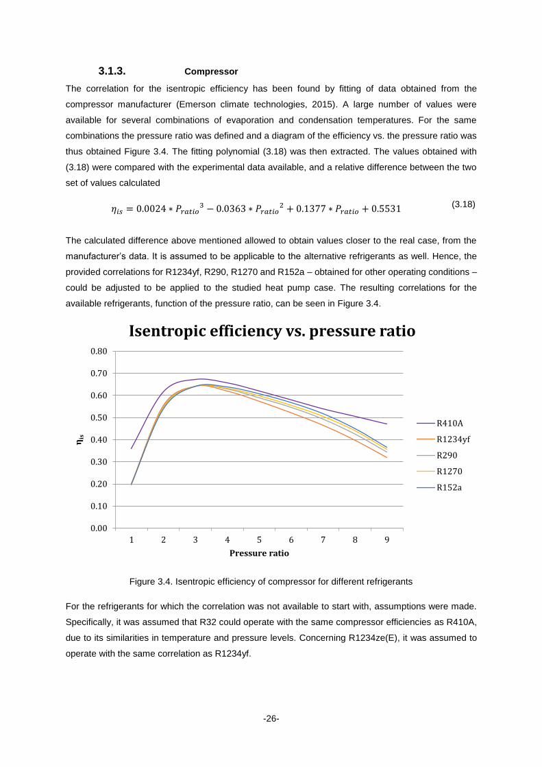
3.1.3. Compressor

The correlation for the isentropic efficiency has been found by fitting of data obtained from the

compressor manufacturer (Emerson climate technologies, 2015). A large number of values were

available for several combinations of evaporation and condensation temperatures. For the same

combinations the pressure ratio was defined and a diagram of the efficiency vs. the pressure ratio was

thus obtained Figure 3.4. The fitting polynomial (3.18) was then extracted. The values obtained with

(3.18) were compared with the experimental data available, and a relative difference between the two

set of values calculated

𝜂𝑖𝑠 = 0.0024 ∗ 𝑃𝑟𝑎𝑡𝑖𝑜3 − 0.0363 ∗ 𝑃𝑟𝑎𝑡𝑖𝑜

2 + 0.1377 ∗ 𝑃𝑟𝑎𝑡𝑖𝑜 + 0.5531 (3.18)

The calculated difference above mentioned allowed to obtain values closer to the real case, from the

manufacturer’s data. It is assumed to be applicable to the alternative refrigerants as well. Hence, the

provided correlations for R1234yf, R290, R1270 and R152a – obtained for other operating conditions –

could be adjusted to be applied to the studied heat pump case. The resulting correlations for the

available refrigerants, function of the pressure ratio, can be seen in Figure 3.4.

Figure 3.4. Isentropic efficiency of compressor for different refrigerants

For the refrigerants for which the correlation was not available to start with, assumptions were made.

Specifically, it was assumed that R32 could operate with the same compressor efficiencies as R410A,

due to its similarities in temperature and pressure levels. Concerning R1234ze(E), it was assumed to

operate with the same correlation as R1234yf.

0.00

0.10

0.20

0.30

0.40

0.50

0.60

0.70

0.80

1 2 3 4 5 6 7 8 9

ηis

Pressure ratio

Isentropic efficiency vs. pressure ratio

R410A

R1234yf

R290

R1270

R152a

-27-

No assumptions regarding the compressor could be made for R450A and R513A, because of the limited

access to data. For this reason, the analysis of these two refrigerants is left for the future steps of the

work.

Concerning the volumetric efficiency of the compressor (ηs), another correlation was elaborated. The

value for the swept volume (�̇�𝑠𝑤𝑒𝑝𝑡) was available for the specific compressor at the given operating

conditions (50 Hz or 3000 rpm) on the Emerson online software (Emerson climate technologies, 2015)

and equals to 6.93 m3/h (0.001925 m3/s).

The relation between the mass flow of the refrigerant and the volumetric efficiency is given by equation

(3.19) (Ekroth, 2011):

�̇�𝑟𝑒𝑓 = 𝜌2 ∗ �̇�𝑠𝑤𝑒𝑝𝑡 ∗ 𝜂𝑠 (3.19)

Where �̇�𝑟𝑒𝑓 is the mass flow of refrigerant in kg/s, 𝜌2 the density of the refrigerant in point 2 of the cycle

in kg/m3, �̇�𝑠𝑤𝑒𝑝𝑡 the swept volume in m3/s and 𝜂𝑠 the volumetric efficiency of the compressor.

With the other data (�̇�𝑟𝑒𝑓 and 𝜌2) issued from the model, 𝜂𝑠 could be calculated for each point, and

related to the corresponding pressure ratio, thus obtaining the correlation seen in (3.20).

𝜂𝑠 = 0.0015 ∗ 𝑃𝑟𝑎𝑡𝑖𝑜2 − 0.0356 ∗ 𝑃𝑟𝑎𝑡𝑖𝑜 + 1.0583 (3.20)

3.1.4. Condenser

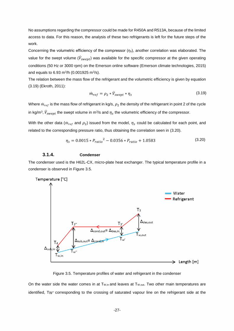
The condenser used is the H62L-CX, micro-plate heat exchanger. The typical temperature profile in a

condenser is observed in Figure 3.5.

Figure 3.5. Temperature profiles of water and refrigerant in the condenser

On the water side the water comes in at TW,in and leaves at TW,out. Two other main temperatures are

identified, TW’’ corresponding to the crossing of saturated vapour line on the refrigerant side at the

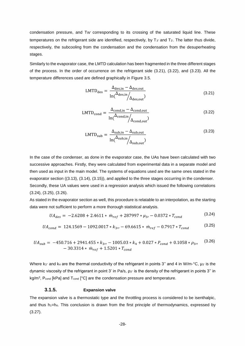
-28-

condensation pressure, and TW’ corresponding to its crossing of the saturated liquid line. These

temperatures on the refrigerant side are identified, respectively, by T3’’ and T3’. The latter thus divide,

respectively, the subcooling from the condensation and the condensation from the desuperheating

stages.

Similarly to the evaporator case, the LMTD calculation has been fragmented in the three different stages

of the process. In the order of occurrence on the refrigerant side (3.21), (3.22), and (3.23). All the

temperature differences used are defined graphically in Figure 3.5.

LMTDdes = Δdes,in − Δdes,out

ln(Δdes,in

Δdes,out⁄ )

(3.21)

LMTDcond = Δcond,in − Δcond,out

ln(Δcond,in

Δcond,out⁄ )

(3.22)

LMTDsub = Δsub,in − Δsub,out

ln(Δsub,in

Δsub,out⁄ )

(3.23)

In the case of the condenser, as done in the evaporator case, the UAs have been calculated with two

successive approaches. Firstly, they were calculated from experimental data in a separate model and

then used as input in the main model. The systems of equations used are the same ones stated in the

evaporator section ((3.13), (3.14), (3.15)), and applied to the three stages occurring in the condenser.

Secondly, these UA values were used in a regression analysis which issued the following correlations

(3.24), (3.25), (3.26).

As stated in the evaporator section as well, this procedure is relatable to an interpolation, as the starting

data were not sufficient to perform a more thorough statistical analysis.

𝑈𝐴𝑑𝑒𝑠 = −2.6208 + 2.4611 ∗ �̇�𝑟𝑒𝑓 + 287997 ∗ 𝜇3′ − 0.0372 ∗ 𝑇𝑐𝑜𝑛𝑑 (3.24)

𝑈𝐴𝑐𝑜𝑛𝑑 = 124.1569 − 1092.0017 ∗ 𝑘3′′ − 69.6615 ∗ �̇�𝑟𝑒𝑓 − 0.7917 ∗ 𝑇𝑐𝑜𝑛𝑑 (3.25)

𝑈𝐴𝑠𝑢𝑏 = −450.716 + 2941.455 ∗ 𝑘3′′ − 1005.03 ∗ 𝑘4 + 0.027 ∗ 𝑃𝑐𝑜𝑛𝑑 + 0.1058 ∗ 𝜌3′′

− 30.3314 ∗ �̇�𝑟𝑒𝑓 + 1.5201 ∗ 𝑇𝑐𝑜𝑛𝑑

(3.26)

Where k3’’ and k4 are the thermal conductivity of the refrigerant in points 3’’ and 4 in W/m-°C, μ3’ is the

dynamic viscosity of the refrigerant in point 3’ in Pa/s, ρ3’’ is the density of the refrigerant in points 3’’ in

kg/m3, Pcond [kPa] and Tcond [°C] are the condensation pressure and temperature.

3.1.5. Expansion valve

The expansion valve is a thermostatic type and the throttling process is considered to be isenthalpic,

and thus h1=h4. This conclusion is drawn from the first principle of thermodynamics, expressed by

(3.27).

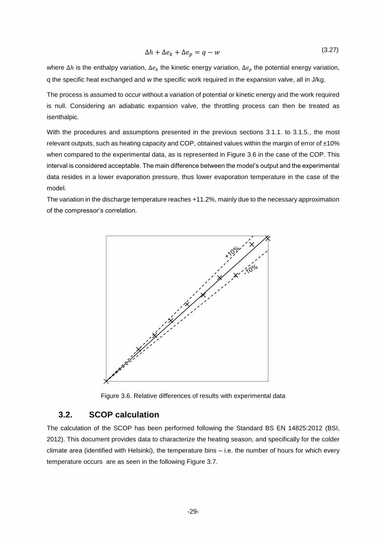
-29-

∆ℎ + ∆𝑒𝑘 + ∆𝑒𝑝 = 𝑞 − 𝑤 (3.27)

where ∆ℎ is the enthalpy variation, ∆𝑒𝑘 the kinetic energy variation, ∆𝑒𝑝 the potential energy variation,

q the specific heat exchanged and w the specific work required in the expansion valve, all in J/kg.

The process is assumed to occur without a variation of potential or kinetic energy and the work required

is null. Considering an adiabatic expansion valve, the throttling process can then be treated as

isenthalpic.

With the procedures and assumptions presented in the previous sections 3.1.1. to 3.1.5., the most

relevant outputs, such as heating capacity and COP, obtained values within the margin of error of ±10%

when compared to the experimental data, as is represented in Figure 3.6 in the case of the COP. This

interval is considered acceptable. The main difference between the model’s output and the experimental

data resides in a lower evaporation pressure, thus lower evaporation temperature in the case of the

model.

The variation in the discharge temperature reaches +11.2%, mainly due to the necessary approximation

of the compressor’s correlation.

Figure 3.6. Relative differences of results with experimental data

3.2. SCOP calculation

The calculation of the SCOP has been performed following the Standard BS EN 14825:2012 (BSI,

2012). This document provides data to characterize the heating season, and specifically for the colder

climate area (identified with Helsinki), the temperature bins – i.e. the number of hours for which every

temperature occurs are as seen in the following Figure 3.7.

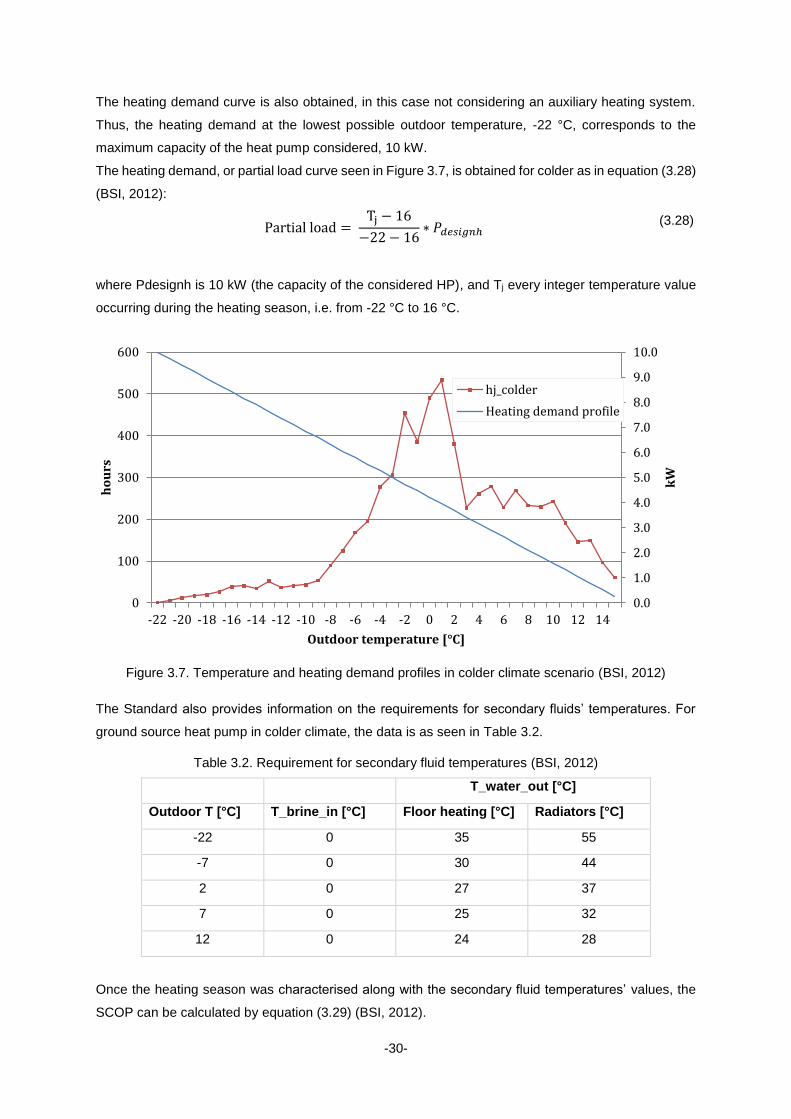
-30-

The heating demand curve is also obtained, in this case not considering an auxiliary heating system.

Thus, the heating demand at the lowest possible outdoor temperature, -22 °C, corresponds to the

maximum capacity of the heat pump considered, 10 kW.

The heating demand, or partial load curve seen in Figure 3.7, is obtained for colder as in equation (3.28)

(BSI, 2012):

Partial load = Tj − 16

−22 − 16∗ 𝑃𝑑𝑒𝑠𝑖𝑔𝑛ℎ

(3.28)

where Pdesignh is 10 kW (the capacity of the considered HP), and Tj every integer temperature value

occurring during the heating season, i.e. from -22 °C to 16 °C.

Figure 3.7. Temperature and heating demand profiles in colder climate scenario (BSI, 2012)

The Standard also provides information on the requirements for secondary fluids’ temperatures. For

ground source heat pump in colder climate, the data is as seen in Table 3.2.

Table 3.2. Requirement for secondary fluid temperatures (BSI, 2012)

T_water_out [°C]

Outdoor T [°C] T_brine_in [°C] Floor heating [°C] Radiators [°C]

-22 0 35 55

-7 0 30 44

2 0 27 37

7 0 25 32

12 0 24 28

Once the heating season was characterised along with the secondary fluid temperatures’ values, the

SCOP can be calculated by equation (3.29) (BSI, 2012).

0.0

1.0

2.0

3.0

4.0

5.0

6.0

7.0

8.0

9.0

10.0

0

100

200

300

400

500

600

-22 -20 -18 -16 -14 -12 -10 -8 -6 -4 -2 0 2 4 6 8 10 12 14

kW

ho

urs

Outdoor temperature [°C]

hj_colder

Heating demand profile

-31-

𝑆𝐶𝑂𝑃𝑂𝑁 = ∑ ℎ𝑗 ∗ 𝑃ℎ(𝑇𝑗)𝑛

𝑗=1

∑ ℎ𝑗 ∗ (𝑃ℎ(𝑇𝑗) − 𝑒𝑙𝑏𝑢(𝑇𝑗)

𝐶𝑂𝑃𝑝𝑎𝑟𝑡𝑖𝑎𝑙(𝑇𝑗)+ 𝑒𝑙𝑏𝑢(𝑇𝑗))𝑛

𝑗=1

(3.29)

Where hj is the number of hours for which the outdoor temperature Tj [°C] occurs, Ph(Tj) is the heating

demand corresponding to the outdoor temperature Tj [kW], elbu(Tj) is the eventual power obtained from

an electric back-up unit [kW], and COPpartial (Tj) is the COP calculated at the specific outdoor

temperature Tj.

In the case of this study, it is assumed that no back-up unit is present.

For the baseline, R410A, the SCOP is calculated as 4.14.

3.3. TEWI calculation

The TEWI factor is calculated according to equation (2.1). A certain number of inputs, besides the GWP

and the SCOP, are required in order to describe the system performance and their first assumed values

are presented in Table 3.3.

Table 3.3. TEWI input parameters

Annual leakage rate 2%/year

Lifetime [years] 15

β [kg CO2/kWhe] 0.023

α recovery 0.7

Charge [kg] 2.3*

Annual heating demand [kWh] 27547.35

* Example of charge value for R410A. The value adjusted for other refrigerants in accordance to the values

presented below.

The input parameters consist of:

Annual leakage rate, in % of the charge of the system.

For a self-contained refrigerating system, the value is assumed at 2% (AIRAH, 2012).

Lifetime of the system, in years

β or CO2 emission factor, in kg CO2/kWhe

The value is based on the average emission of the electricity sector of a country or area, thus is

dependent on the energy mix of the considered location. In Sweden this factor is equal to 0.023 kg

CO2/kWhe (Convenant of Mayors, 2012).

α or recovery efficiency, from 0 to 1

It indicates the proportion of refrigerant charge that is recovered from a system when decommissioned.

Chosen by default at 0.7.

-32-

The charge, in L or m3

The quantity of charge in kg is known from the experimental data, and equals 2.3 kg of R410A. Through

its specific volume at the temperature range operated by the machine, the charge in volume was

obtained. When considering the other alternative refrigerants, a constant volumetric charge was

assumed, in order to obtain different mass values by the means of the specific volumes (Table 3.4).

Table 3.4. Charge values by refrigerant

Refrigerant sp. volume [L/kg] Charge [kg]

R410A 1.05 2.300

R32 1.07 2.257

R152a 1.15 2.100

R290 2.10 1.150

R1270 0.56 4.275

R1234yf 0.91 2.657

R1234ze(E) 0.90 2.683

The annual heating demand, in kWh

The value is calculated from the guidelines given by the Standard BS EN 14825:2012 (BSI, 2012) and

is used in order to obtain the energy consumption per year Eannual, in kWh/year, through equation (3.30).

𝐸𝑎𝑛𝑛𝑢𝑎𝑙

=𝑇𝑜𝑡𝑎𝑙 ℎ𝑒𝑎𝑡𝑖𝑛𝑔 𝑑𝑒𝑚𝑎𝑛𝑑

𝑆𝐶𝑂𝑃⁄ (3.30)

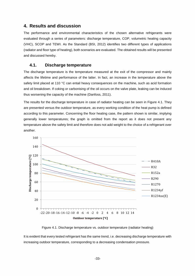
-33-

4. Results and discussion

The performance and environmental characteristics of the chosen alternative refrigerants were

evaluated through a series of parameters: discharge temperature, COP, volumetric heating capacity

(VHC), SCOP and TEWI. As the Standard (BSI, 2012) identifies two different types of applications

(radiator and floor type of heating), both scenarios are evaluated. The obtained results will be presented

and discussed hereby.

4.1. Discharge temperature

The discharge temperature is the temperature measured at the exit of the compressor and mainly

affects the lifetime and performance of the latter. In fact, an increase in the temperature above the

safety limit placed at 110 °C can entail heavy consequences on the machine, such as acid formation

and oil breakdown. If coking or carbonising of the oil occurs on the valve plate, leaking can be induced

thus worsening the capacity of the machine (Danfoss, 2011).

The results for the discharge temperature in case of radiator heating can be seen in Figure 4.1. They

are presented versus the outdoor temperature, as every working condition of the heat pump is defined

according to this parameter. Concerning the floor heating case, the pattern shown is similar, implying

generally lower temperatures; the graph is omitted from the report as it does not present any

temperature above the safety limit and therefore does not add weight to the choice of a refrigerant over

another.

Figure 4.1. Discharge temperature vs. outdoor temperature (radiator heating)

It is evident that every tested refrigerant has the same trend, i.e. decreasing discharge temperature with

increasing outdoor temperature, corresponding to a decreasing condensation pressure.

0

20

40

60

80

100

120

140

160

-22-20-18-16-14-12-10 -8 -6 -4 -2 0 2 4 6 8 10 12 14

Dis

cha

rge

te

mp

era

ture

[°C

]


R410A

R32

R152a

R290

R1270

R1234yf

R1234ze(E)

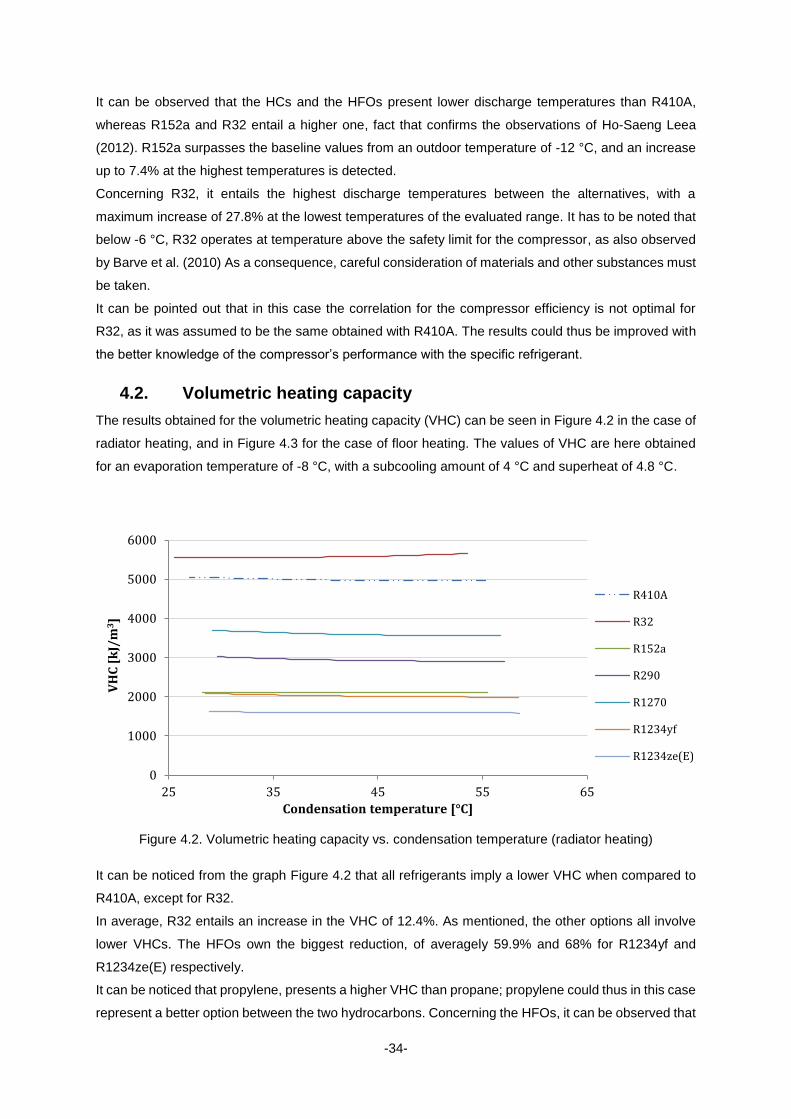
-34-

It can be observed that the HCs and the HFOs present lower discharge temperatures than R410A,

whereas R152a and R32 entail a higher one, fact that confirms the observations of Ho-Saeng Leea

(2012). R152a surpasses the baseline values from an outdoor temperature of -12 °C, and an increase

up to 7.4% at the highest temperatures is detected.

Concerning R32, it entails the highest discharge temperatures between the alternatives, with a

maximum increase of 27.8% at the lowest temperatures of the evaluated range. It has to be noted that

below -6 °C, R32 operates at temperature above the safety limit for the compressor, as also observed

by Barve et al. (2010) As a consequence, careful consideration of materials and other substances must

be taken.

It can be pointed out that in this case the correlation for the compressor efficiency is not optimal for

R32, as it was assumed to be the same obtained with R410A. The results could thus be improved with

the better knowledge of the compressor’s performance with the specific refrigerant.

4.2. Volumetric heating capacity

The results obtained for the volumetric heating capacity (VHC) can be seen in Figure 4.2 in the case of

radiator heating, and in Figure 4.3 for the case of floor heating. The values of VHC are here obtained

for an evaporation temperature of -8 °C, with a subcooling amount of 4 °C and superheat of 4.8 °C.

Figure 4.2. Volumetric heating capacity vs. condensation temperature (radiator heating)

It can be noticed from the graph Figure 4.2 that all refrigerants imply a lower VHC when compared to

R410A, except for R32.

In average, R32 entails an increase in the VHC of 12.4%. As mentioned, the other options all involve

lower VHCs. The HFOs own the biggest reduction, of averagely 59.9% and 68% for R1234yf and

R1234ze(E) respectively.

It can be noticed that propylene, presents a higher VHC than propane; propylene could thus in this case

represent a better option between the two hydrocarbons. Concerning the HFOs, it can be observed that

0

1000

2000

3000

4000

5000

6000

25 35 45 55 65

VH

C [

kJ/

m3]

Condensation temperature [°C]

R410A

R32

R152a

R290

R1270

R1234yf

R1234ze(E)

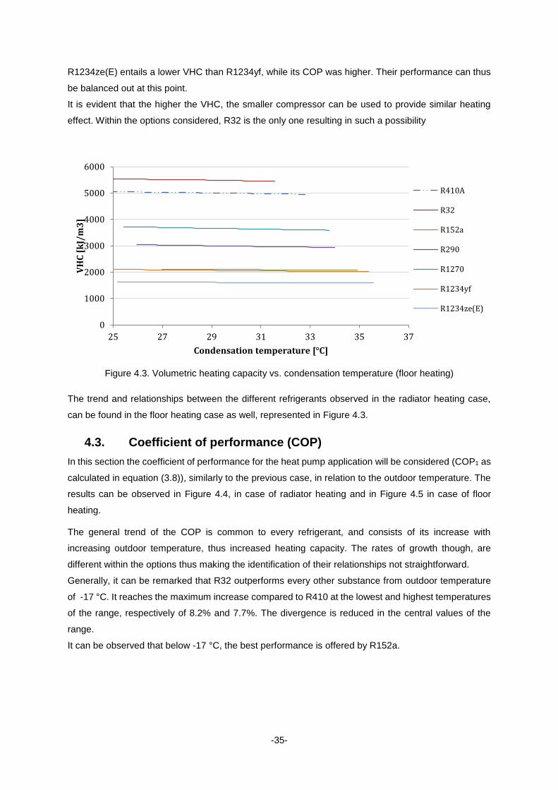
-35-

R1234ze(E) entails a lower VHC than R1234yf, while its COP was higher. Their performance can thus

be balanced out at this point.

It is evident that the higher the VHC, the smaller compressor can be used to provide similar heating

effect. Within the options considered, R32 is the only one resulting in such a possibility

Figure 4.3. Volumetric heating capacity vs. condensation temperature (floor heating)

The trend and relationships between the different refrigerants observed in the radiator heating case,

can be found in the floor heating case as well, represented in Figure 4.3.

4.3. Coefficient of performance (COP)

In this section the coefficient of performance for the heat pump application will be considered (COP1 as

calculated in equation (3.8)), similarly to the previous case, in relation to the outdoor temperature. The

results can be observed in Figure 4.4, in case of radiator heating and in Figure 4.5 in case of floor

heating.

The general trend of the COP is common to every refrigerant, and consists of its increase with

increasing outdoor temperature, thus increased heating capacity. The rates of growth though, are

different within the options thus making the identification of their relationships not straightforward.

Generally, it can be remarked that R32 outperforms every other substance from outdoor temperature

of -17 °C. It reaches the maximum increase compared to R410 at the lowest and highest temperatures

of the range, respectively of 8.2% and 7.7%. The divergence is reduced in the central values of the

range.

It can be observed that below -17 °C, the best performance is offered by R152a.

0

1000

2000

3000

4000

5000

6000

25 27 29 31 33 35 37

VH

C [

kJ/

m3

]

Condensation temperature [°C]

R410A

R32

R152a

R290

R1270

R1234yf

R1234ze(E)

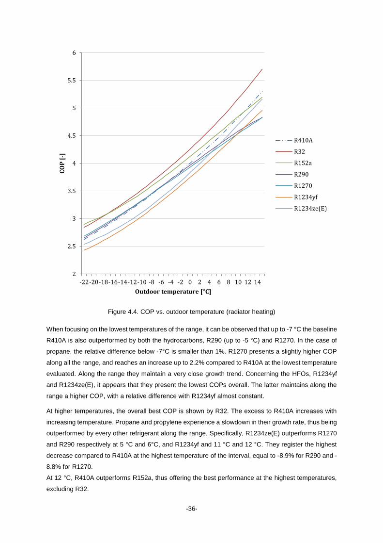
-36-

Figure 4.4. COP vs. outdoor temperature (radiator heating)

When focusing on the lowest temperatures of the range, it can be observed that up to -7 °C the baseline

R410A is also outperformed by both the hydrocarbons, R290 (up to -5 °C) and R1270. In the case of

propane, the relative difference below -7°C is smaller than 1%. R1270 presents a slightly higher COP

along all the range, and reaches an increase up to 2.2% compared to R410A at the lowest temperature

evaluated. Along the range they maintain a very close growth trend. Concerning the HFOs, R1234yf

and R1234ze(E), it appears that they present the lowest COPs overall. The latter maintains along the

range a higher COP, with a relative difference with R1234yf almost constant.

At higher temperatures, the overall best COP is shown by R32. The excess to R410A increases with

increasing temperature. Propane and propylene experience a slowdown in their growth rate, thus being

outperformed by every other refrigerant along the range. Specifically, R1234ze(E) outperforms R1270

and R290 respectively at 5 °C and 6°C, and R1234yf and 11 °C and 12 °C. They register the highest

decrease compared to R410A at the highest temperature of the interval, equal to -8.9% for R290 and -

8.8% for R1270.

At 12 °C, R410A outperforms R152a, thus offering the best performance at the highest temperatures,

excluding R32.

2

2.5

3

3.5

4

4.5

5

5.5

6

-22-20-18-16-14-12-10 -8 -6 -4 -2 0 2 4 6 8 10 12 14

CO

P [

-]


R410A

R32

R152a

R290

R1270

R1234yf

R1234ze(E)

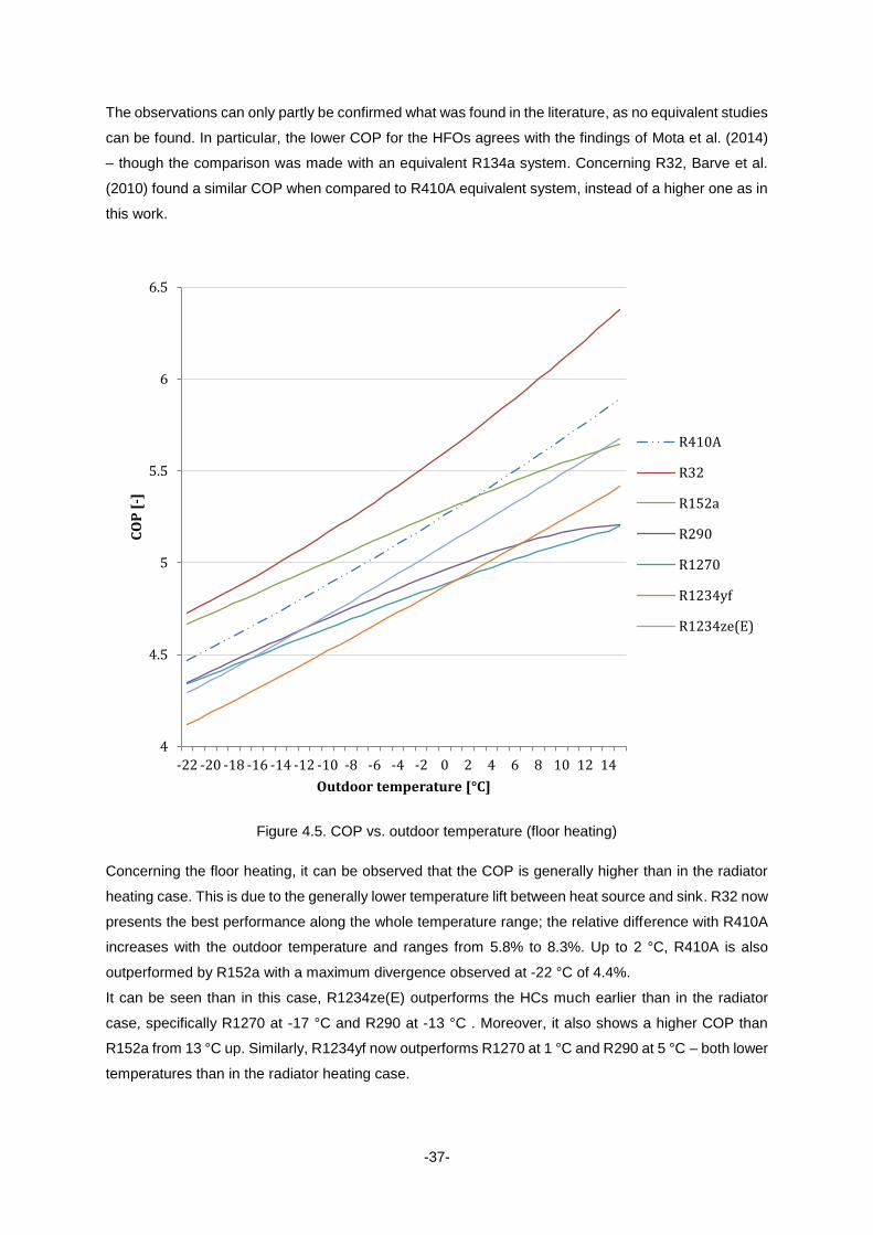
-37-

The observations can only partly be confirmed what was found in the literature, as no equivalent studies

can be found. In particular, the lower COP for the HFOs agrees with the findings of Mota et al. (2014)

– though the comparison was made with an equivalent R134a system. Concerning R32, Barve et al.

(2010) found a similar COP when compared to R410A equivalent system, instead of a higher one as in

this work.

Figure 4.5. COP vs. outdoor temperature (floor heating)

Concerning the floor heating, it can be observed that the COP is generally higher than in the radiator

heating case. This is due to the generally lower temperature lift between heat source and sink. R32 now

presents the best performance along the whole temperature range; the relative difference with R410A

increases with the outdoor temperature and ranges from 5.8% to 8.3%. Up to 2 °C, R410A is also

outperformed by R152a with a maximum divergence observed at -22 °C of 4.4%.

It can be seen than in this case, R1234ze(E) outperforms the HCs much earlier than in the radiator

case, specifically R1270 at -17 °C and R290 at -13 °C . Moreover, it also shows a higher COP than

R152a from 13 °C up. Similarly, R1234yf now outperforms R1270 at 1 °C and R290 at 5 °C – both lower

temperatures than in the radiator heating case.

4

4.5

5

5.5

6

6.5

-22 -20 -18 -16 -14 -12 -10 -8 -6 -4 -2 0 2 4 6 8 10 12 14

CO

P [

-]


R410A

R32

R152a

R290

R1270

R1234yf

R1234ze(E)

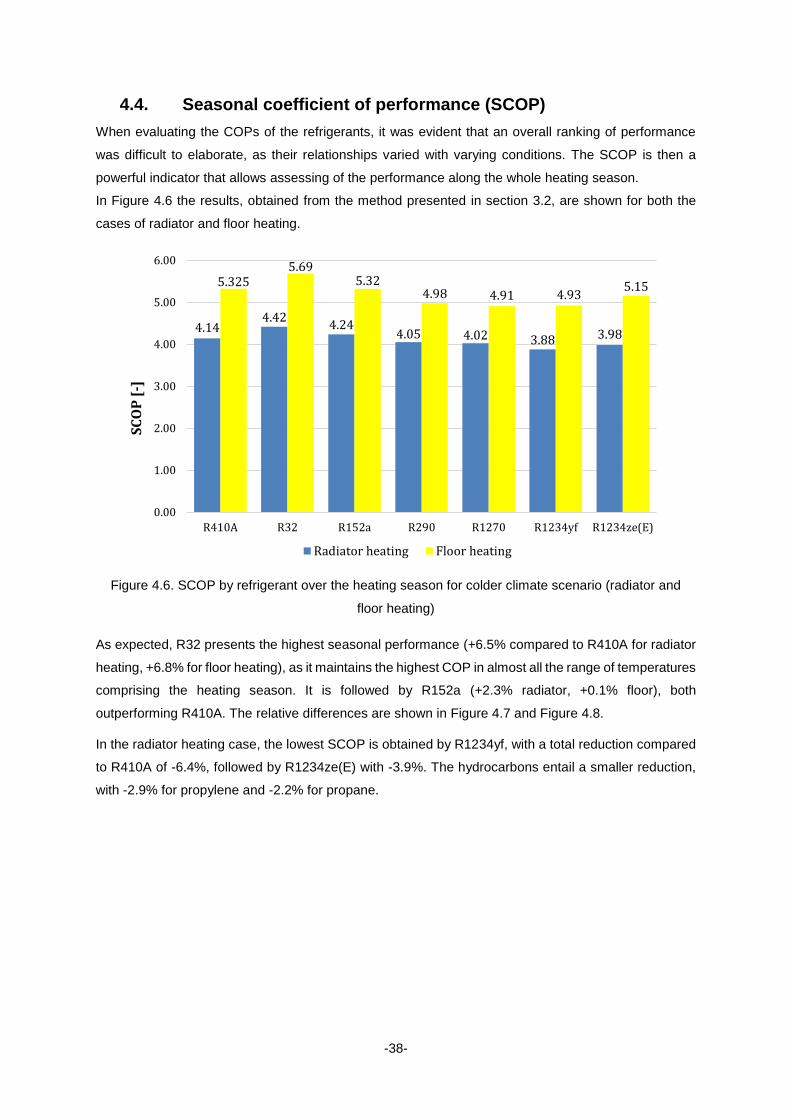
-38-

4.4. Seasonal coefficient of performance (SCOP)

When evaluating the COPs of the refrigerants, it was evident that an overall ranking of performance

was difficult to elaborate, as their relationships varied with varying conditions. The SCOP is then a

powerful indicator that allows assessing of the performance along the whole heating season.

In Figure 4.6 the results, obtained from the method presented in section 3.2, are shown for both the

cases of radiator and floor heating.

Figure 4.6. SCOP by refrigerant over the heating season for colder climate scenario (radiator and

floor heating)

As expected, R32 presents the highest seasonal performance (+6.5% compared to R410A for radiator

heating, +6.8% for floor heating), as it maintains the highest COP in almost all the range of temperatures

comprising the heating season. It is followed by R152a (+2.3% radiator, +0.1% floor), both

outperforming R410A. The relative differences are shown in Figure 4.7 and Figure 4.8.

In the radiator heating case, the lowest SCOP is obtained by R1234yf, with a total reduction compared

to R410A of -6.4%, followed by R1234ze(E) with -3.9%. The hydrocarbons entail a smaller reduction,

with -2.9% for propylene and -2.2% for propane.

4.144.42

4.244.05 4.02 3.88 3.98

5.3255.69

5.324.98 4.91 4.93

5.15

0.00

1.00

2.00

3.00

4.00

5.00

6.00

R410A R32 R152a R290 R1270 R1234yf R1234ze(E)

SC

OP

[-]

Radiator heating Floor heating

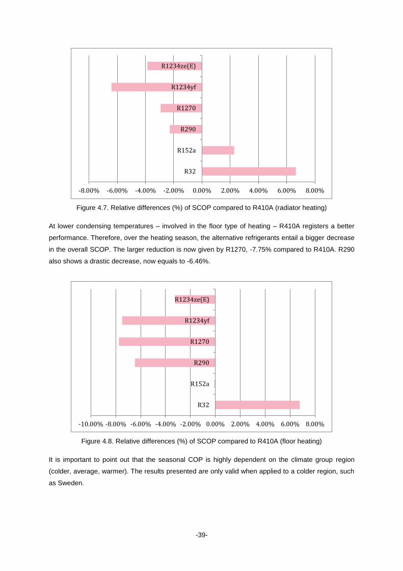
-39-

Figure 4.7. Relative differences (%) of SCOP compared to R410A (radiator heating)

At lower condensing temperatures – involved in the floor type of heating – R410A registers a better

performance. Therefore, over the heating season, the alternative refrigerants entail a bigger decrease

in the overall SCOP. The larger reduction is now given by R1270, -7.75% compared to R410A. R290

also shows a drastic decrease, now equals to -6.46%.

Figure 4.8. Relative differences (%) of SCOP compared to R410A (floor heating)

It is important to point out that the seasonal COP is highly dependent on the climate group region

(colder, average, warmer). The results presented are only valid when applied to a colder region, such

as Sweden.

-8.00% -6.00% -4.00% -2.00% 0.00% 2.00% 4.00% 6.00% 8.00%

R32

R152a

R290

R1270

R1234yf

R1234ze(E)

-10.00% -8.00% -6.00% -4.00% -2.00% 0.00% 2.00% 4.00% 6.00% 8.00%

R32

R152a

R290

R1270

R1234yf

R1234ze(E)

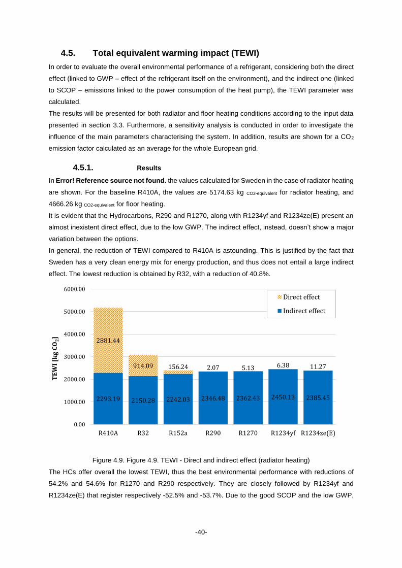
-40-

4.5. Total equivalent warming impact (TEWI)

In order to evaluate the overall environmental performance of a refrigerant, considering both the direct

effect (linked to GWP – effect of the refrigerant itself on the environment), and the indirect one (linked

to SCOP – emissions linked to the power consumption of the heat pump), the TEWI parameter was

calculated.

The results will be presented for both radiator and floor heating conditions according to the input data

presented in section 3.3. Furthermore, a sensitivity analysis is conducted in order to investigate the

influence of the main parameters characterising the system. In addition, results are shown for a CO2

emission factor calculated as an average for the whole European grid.

4.5.1. Results

In Error! Reference source not found. the values calculated for Sweden in the case of radiator heating

are shown. For the baseline R410A, the values are 5174.63 kg CO2-equivalent for radiator heating, and

4666.26 kg CO2-equivalent for floor heating.

It is evident that the Hydrocarbons, R290 and R1270, along with R1234yf and R1234ze(E) present an

almost inexistent direct effect, due to the low GWP. The indirect effect, instead, doesn’t show a major

variation between the options.

In general, the reduction of TEWI compared to R410A is astounding. This is justified by the fact that

Sweden has a very clean energy mix for energy production, and thus does not entail a large indirect

effect. The lowest reduction is obtained by R32, with a reduction of 40.8%.

Figure 4.9. Figure 4.9. TEWI - Direct and indirect effect (radiator heating)

The HCs offer overall the lowest TEWI, thus the best environmental performance with reductions of

54.2% and 54.6% for R1270 and R290 respectively. They are closely followed by R1234yf and

R1234ze(E) that register respectively -52.5% and -53.7%. Due to the good SCOP and the low GWP,

2293.19 2150.28 2242.03 2346.48 2362.43 2450.13 2385.45

2881.44

914.09 156.24 2.07 5.13 6.38 11.27

0.00

1000.00

2000.00

3000.00

4000.00

5000.00

6000.00

R410A R32 R152a R290 R1270 R1234yf R1234ze(E)

TE

WI

[kg

CO

2]

Direct effect

Indirect effect

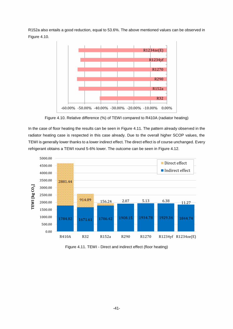
-41-

R152a also entails a good reduction, equal to 53.6%. The above mentioned values can be observed in

Figure 4.10.

Figure 4.10. Relative difference (%) of TEWI compared to R410A (radiator heating)

In the case of floor heating the results can be seen in Figure 4.11. The pattern already observed in the

radiator heating case is respected in this case already. Due to the overall higher SCOP values, the

TEWI is generally lower thanks to a lower indirect effect. The direct effect is of course unchanged. Every

refrigerant obtains a TEWI round 5-6% lower. The outcome can be seen in Figure 4.12.

Figure 4.11. TEWI - Direct and indirect effect (floor heating)

-60.00% -50.00% -40.00% -30.00% -20.00% -10.00% 0.00%

R32

R152a

R290

R1270

R1234yf

R1234ze(E)

1784.82 1671.61 1786.42 1908.15 1934.78 1929.34 1844.74

2881.44

914.09 156.24 2.07 5.13 6.38 11.27

0.00

500.00

1000.00

1500.00

2000.00

2500.00

3000.00

3500.00

4000.00

4500.00

5000.00

R410A R32 R152a R290 R1270 R1234yf R1234ze(E)

TE

WI

[kg

CO

2]

Direct effect

Indirect effect

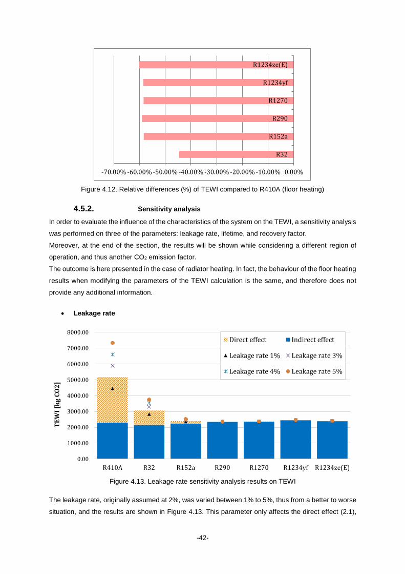
-42-

Figure 4.12. Relative differences (%) of TEWI compared to R410A (floor heating)

4.5.2. Sensitivity analysis

In order to evaluate the influence of the characteristics of the system on the TEWI, a sensitivity analysis

was performed on three of the parameters: leakage rate, lifetime, and recovery factor.

Moreover, at the end of the section, the results will be shown while considering a different region of

operation, and thus another CO2 emission factor.

The outcome is here presented in the case of radiator heating. In fact, the behaviour of the floor heating

results when modifying the parameters of the TEWI calculation is the same, and therefore does not

provide any additional information.

Leakage rate

Figure 4.13. Leakage rate sensitivity analysis results on TEWI

The leakage rate, originally assumed at 2%, was varied between 1% to 5%, thus from a better to worse

situation, and the results are shown in Figure 4.13. This parameter only affects the direct effect (2.1),

-70.00% -60.00% -50.00% -40.00% -30.00% -20.00% -10.00% 0.00%

R32

R152a

R290

R1270

R1234yf

R1234ze(E)

0.00

1000.00

2000.00

3000.00

4000.00

5000.00

6000.00

7000.00

8000.00

R410A R32 R152a R290 R1270 R1234yf R1234ze(E)

TE

WI

[kg

CO

2]

Direct effect Indirect effect

Leakage rate 1% Leakage rate 3%

Leakage rate 4% Leakage rate 5%

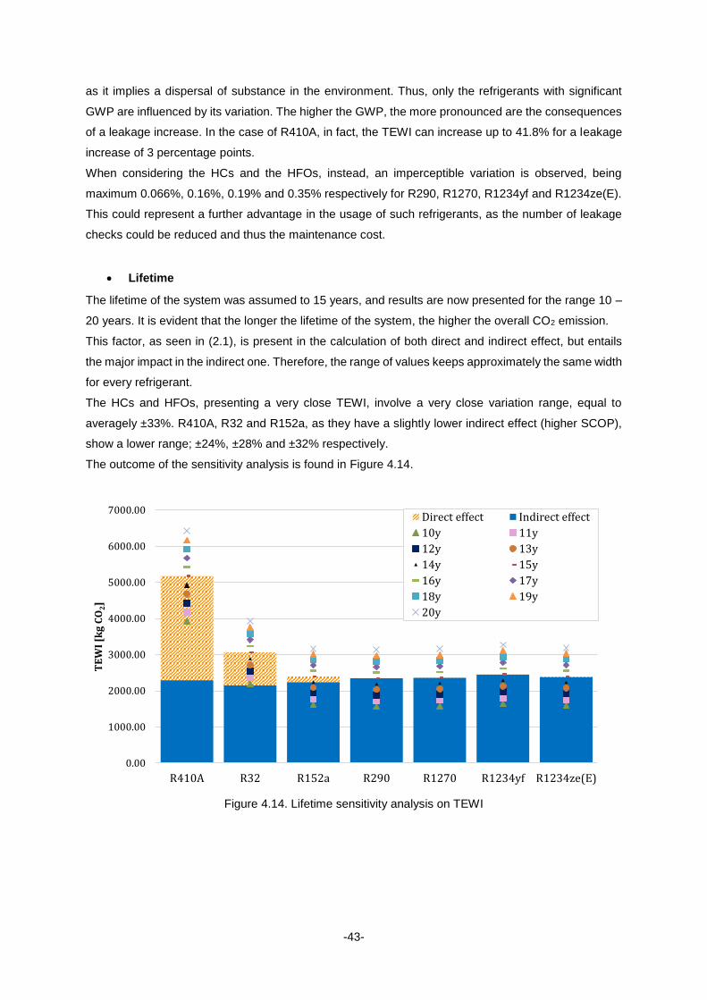
-43-

as it implies a dispersal of substance in the environment. Thus, only the refrigerants with significant

GWP are influenced by its variation. The higher the GWP, the more pronounced are the consequences

of a leakage increase. In the case of R410A, in fact, the TEWI can increase up to 41.8% for a leakage

increase of 3 percentage points.

When considering the HCs and the HFOs, instead, an imperceptible variation is observed, being

maximum 0.066%, 0.16%, 0.19% and 0.35% respectively for R290, R1270, R1234yf and R1234ze(E).

This could represent a further advantage in the usage of such refrigerants, as the number of leakage

checks could be reduced and thus the maintenance cost.

Lifetime

The lifetime of the system was assumed to 15 years, and results are now presented for the range 10 –

20 years. It is evident that the longer the lifetime of the system, the higher the overall CO2 emission.

This factor, as seen in (2.1), is present in the calculation of both direct and indirect effect, but entails

the major impact in the indirect one. Therefore, the range of values keeps approximately the same width

for every refrigerant.

The HCs and HFOs, presenting a very close TEWI, involve a very close variation range, equal to

averagely ±33%. R410A, R32 and R152a, as they have a slightly lower indirect effect (higher SCOP),

show a lower range; ±24%, ±28% and ±32% respectively.

The outcome of the sensitivity analysis is found in Figure 4.14.

Figure 4.14. Lifetime sensitivity analysis on TEWI

0.00

1000.00

2000.00

3000.00

4000.00

5000.00

6000.00

7000.00

R410A R32 R152a R290 R1270 R1234yf R1234ze(E)

TE

WI

[kg

CO

2]


10y 11y

12y 13y

14y 15y

16y 17y

18y 19y

20y

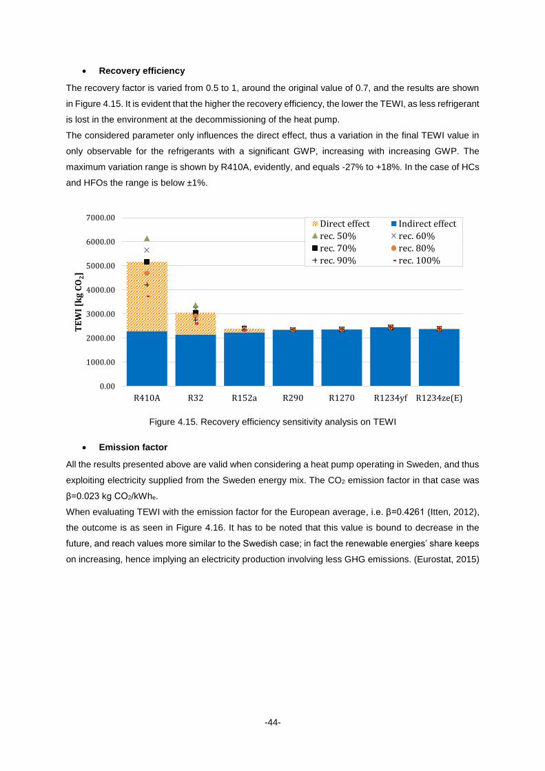
-44-

Recovery efficiency

The recovery factor is varied from 0.5 to 1, around the original value of 0.7, and the results are shown

in Figure 4.15. It is evident that the higher the recovery efficiency, the lower the TEWI, as less refrigerant

is lost in the environment at the decommissioning of the heat pump.

The considered parameter only influences the direct effect, thus a variation in the final TEWI value in

only observable for the refrigerants with a significant GWP, increasing with increasing GWP. The

maximum variation range is shown by R410A, evidently, and equals -27% to +18%. In the case of HCs

and HFOs the range is below ±1%.

Figure 4.15. Recovery efficiency sensitivity analysis on TEWI

Emission factor

All the results presented above are valid when considering a heat pump operating in Sweden, and thus

exploiting electricity supplied from the Sweden energy mix. The CO2 emission factor in that case was

β=0.023 kg CO2/kWhe.

When evaluating TEWI with the emission factor for the European average, i.e. β=0.4261 (Itten, 2012),

the outcome is as seen in Figure 4.16. It has to be noted that this value is bound to decrease in the

future, and reach values more similar to the Swedish case; in fact the renewable energies’ share keeps

on increasing, hence implying an electricity production involving less GHG emissions. (Eurostat, 2015)

0.00

1000.00

2000.00

3000.00

4000.00

5000.00

6000.00

7000.00

R410A R32 R152a R290 R1270 R1234yf R1234ze(E)

TE

WI

[kg

CO

2]


rec. 50% rec. 60%

rec. 70% rec. 80%

rec. 90% rec. 100%

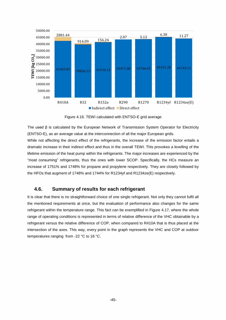
-45-

Figure 4.16. TEWI calculated with ENTSO-E grid average

The used β is calculated by the European Network of Transmission System Operator for Electricity

(ENTSO-E), as an average value at the interconnection of all the major European grids.

While not affecting the direct effect of the refrigerants, the increase of the emission factor entails a

dramatic increase in their indirect effect and thus in the overall TEWI. This provokes a levelling of the

lifetime emission of the heat pump within the refrigerants. The major increases are experienced by the

“most consuming” refrigerants, thus the ones with lower SCOP. Specifically, the HCs measure an

increase of 1751% and 1748% for propane and propylene respectively. They are closely followed by

the HFOs that augment of 1748% and 1744% for R1234yf and R1234ze(E) respectively.

4.6. Summary of results for each refrigerant

It is clear that there is no straightforward choice of one single refrigerant. Not only they cannot fulfil all

the mentioned requirements at once, but the evaluation of performance also changes for the same

refrigerant within the temperature range. This fact can be exemplified in Figure 4.17, where the whole

range of operating conditions is represented in terms of relative difference of the VHC obtainable by a

refrigerant versus the relative difference of COP, when compared to R410A that is thus placed at the

intersection of the axes. This way, every point in the graph represents the VHC and COP at outdoor

temperatures ranging from -22 °C to 16 °C.

42483.8339836.23 41536.12 43471.08 43766.65 45391.28 44193.11

2881.44

914.09 156.242.07 5.13

6.38 11.27

0.00

5000.00

10000.00

15000.00

20000.00

25000.00

30000.00

35000.00

40000.00

45000.00

50000.00

R410A R32 R152a R290 R1270 R1234yf R1234ze(E)

TE

WI

[kg

CO

2]

Indirect effect Direct effect

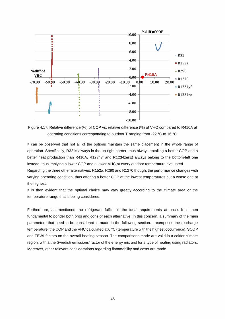
-46-

Figure 4.17. Relative difference (%) of COP vs. relative difference (%) of VHC compared to R410A at

operating conditions corresponding to outdoor T ranging from -22 °C to 16 °C.

It can be observed that not all of the options maintain the same placement in the whole range of

operation. Specifically, R32 is always in the up-right corner, thus always entailing a better COP and a

better heat production than R410A. R1234yf and R1234ze(E) always belong to the bottom-left one

instead, thus implying a lower COP and a lower VHC at every outdoor temperature evaluated.

Regarding the three other alternatives, R152a, R290 and R1270 though, the performance changes with

varying operating condition, thus offering a better COP at the lowest temperatures but a worse one at

the highest.

It is then evident that the optimal choice may vary greatly according to the climate area or the

temperature range that is being considered.

Furthermore, as mentioned, no refrigerant fulfils all the ideal requirements at once. It is then

fundamental to ponder both pros and cons of each alternative. In this concern, a summary of the main

parameters that need to be considered is made in the following section. It comprises the discharge

temperature, the COP and the VHC calculated at 0 °C (temperature with the highest occurrence), SCOP

and TEWI factors on the overall heating season. The comparisons made are valid in a colder climate

region, with a the Swedish emissions’ factor of the energy mix and for a type of heating using radiators.

Moreover, other relevant considerations regarding flammability and costs are made.

-10.00

-8.00

-6.00

-4.00

-2.00

0.00

2.00

4.00

6.00

8.00

10.00

-70.00 -60.00 -50.00 -40.00 -30.00 -20.00 -10.00 0.00 10.00 20.00

%diff of COP

%diff of VHC

R32

R152a

R290

R1270

R1234yf

R1234ze

R410A

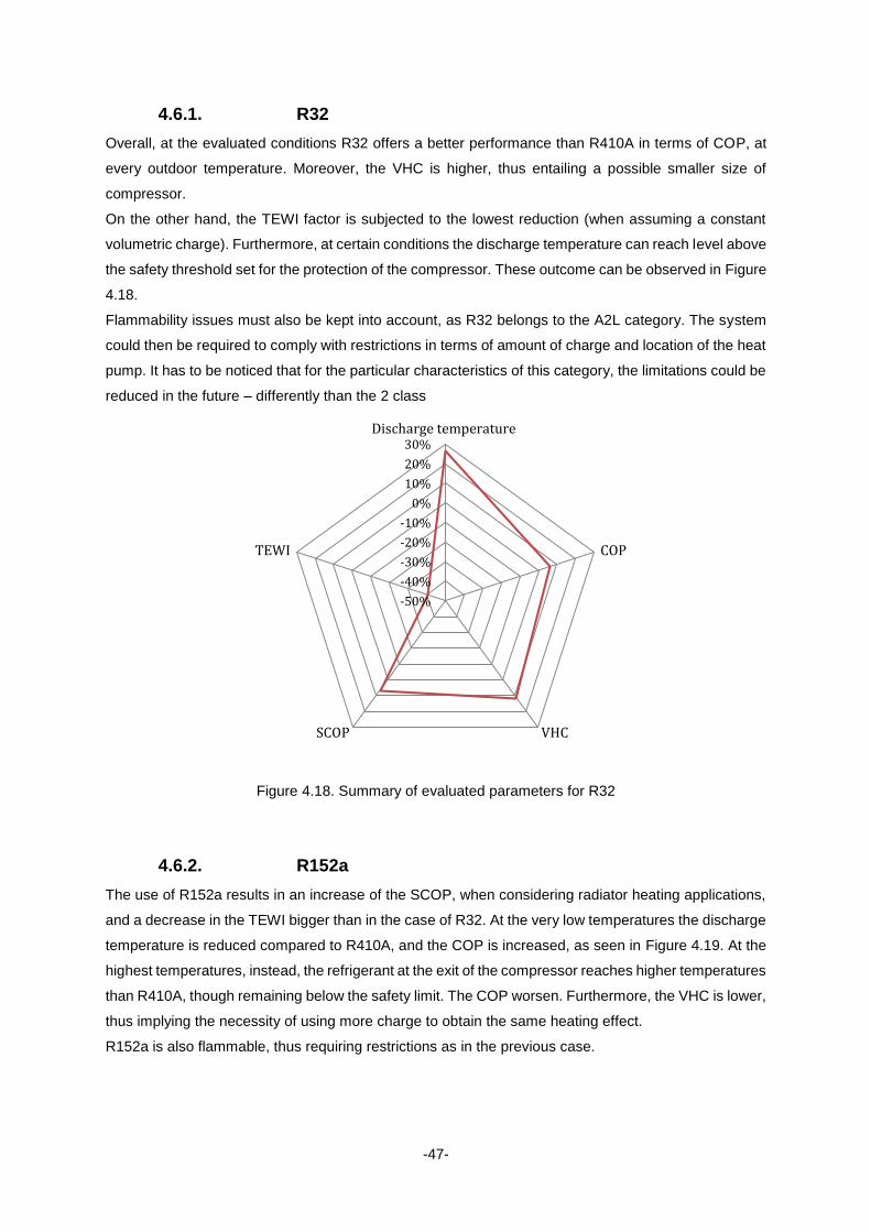
-47-

4.6.1. R32

Overall, at the evaluated conditions R32 offers a better performance than R410A in terms of COP, at

every outdoor temperature. Moreover, the VHC is higher, thus entailing a possible smaller size of

compressor.

On the other hand, the TEWI factor is subjected to the lowest reduction (when assuming a constant

volumetric charge). Furthermore, at certain conditions the discharge temperature can reach level above

the safety threshold set for the protection of the compressor. These outcome can be observed in Figure

4.18.

Flammability issues must also be kept into account, as R32 belongs to the A2L category. The system

could then be required to comply with restrictions in terms of amount of charge and location of the heat

pump. It has to be noticed that for the particular characteristics of this category, the limitations could be

reduced in the future – differently than the 2 class

Figure 4.18. Summary of evaluated parameters for R32

4.6.2. R152a

The use of R152a results in an increase of the SCOP, when considering radiator heating applications,

and a decrease in the TEWI bigger than in the case of R32. At the very low temperatures the discharge

temperature is reduced compared to R410A, and the COP is increased, as seen in Figure 4.19. At the

highest temperatures, instead, the refrigerant at the exit of the compressor reaches higher temperatures

than R410A, though remaining below the safety limit. The COP worsen. Furthermore, the VHC is lower,

thus implying the necessity of using more charge to obtain the same heating effect.

R152a is also flammable, thus requiring restrictions as in the previous case.

-50%

-40%

-30%

-20%

-10%

0%

10%

20%

30%Discharge temperature

COP

VHCSCOP

TEWI

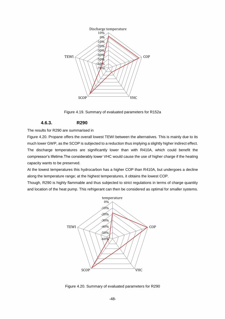
-48-

Figure 4.19. Summary of evaluated parameters for R152a

4.6.3. R290

The results for R290 are summarised in

Figure 4.20. Propane offers the overall lowest TEWI between the alternatives. This is mainly due to its

much lower GWP, as the SCOP is subjected to a reduction thus implying a slightly higher indirect effect.

The discharge temperatures are significantly lower than with R410A, which could benefit the

compressor’s lifetime.The considerably lower VHC would cause the use of higher charge if the heating

capacity wants to be preserved.

At the lowest temperatures this hydrocarbon has a higher COP than R410A, but undergoes a decline

along the temperature range; at the highest temperatures, it obtains the lowest COP.

Though, R290 is highly flammable and thus subjected to strict regulations in terms of charge quantity

and location of the heat pump. This refrigerant can then be considered as optimal for smaller systems.


-70%

-60%

-50%

-40%

-30%

-20%

-10%

0%


COP

VHCSCOP

TEWI

-60%

-50%

-40%

-30%

-20%

-10%

0%

Dischargetemperature

COP

VHCSCOP

TEWI

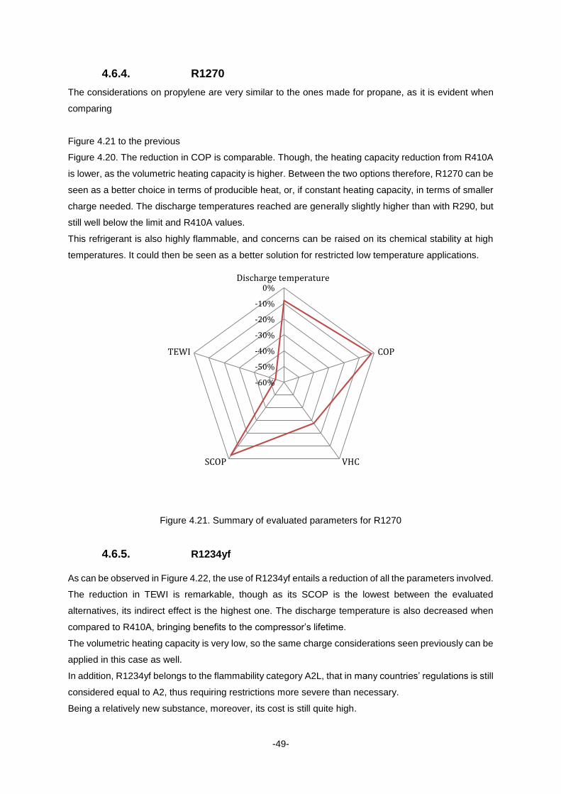
-49-

4.6.4. R1270

The considerations on propylene are very similar to the ones made for propane, as it is evident when

comparing

Figure 4.21 to the previous

Figure 4.20. The reduction in COP is comparable. Though, the heating capacity reduction from R410A

is lower, as the volumetric heating capacity is higher. Between the two options therefore, R1270 can be

seen as a better choice in terms of producible heat, or, if constant heating capacity, in terms of smaller

charge needed. The discharge temperatures reached are generally slightly higher than with R290, but

still well below the limit and R410A values.

This refrigerant is also highly flammable, and concerns can be raised on its chemical stability at high

temperatures. It could then be seen as a better solution for restricted low temperature applications.


4.6.5. R1234yf

As can be observed in Figure 4.22, the use of R1234yf entails a reduction of all the parameters involved.

The reduction in TEWI is remarkable, though as its SCOP is the lowest between the evaluated

alternatives, its indirect effect is the highest one. The discharge temperature is also decreased when

compared to R410A, bringing benefits to the compressor’s lifetime.

The volumetric heating capacity is very low, so the same charge considerations seen previously can be

applied in this case as well.

In addition, R1234yf belongs to the flammability category A2L, that in many countries’ regulations is still

considered equal to A2, thus requiring restrictions more severe than necessary.

Being a relatively new substance, moreover, its cost is still quite high.

-60%

-50%

-40%

-30%

-20%

-10%


COP

VHCSCOP

TEWI

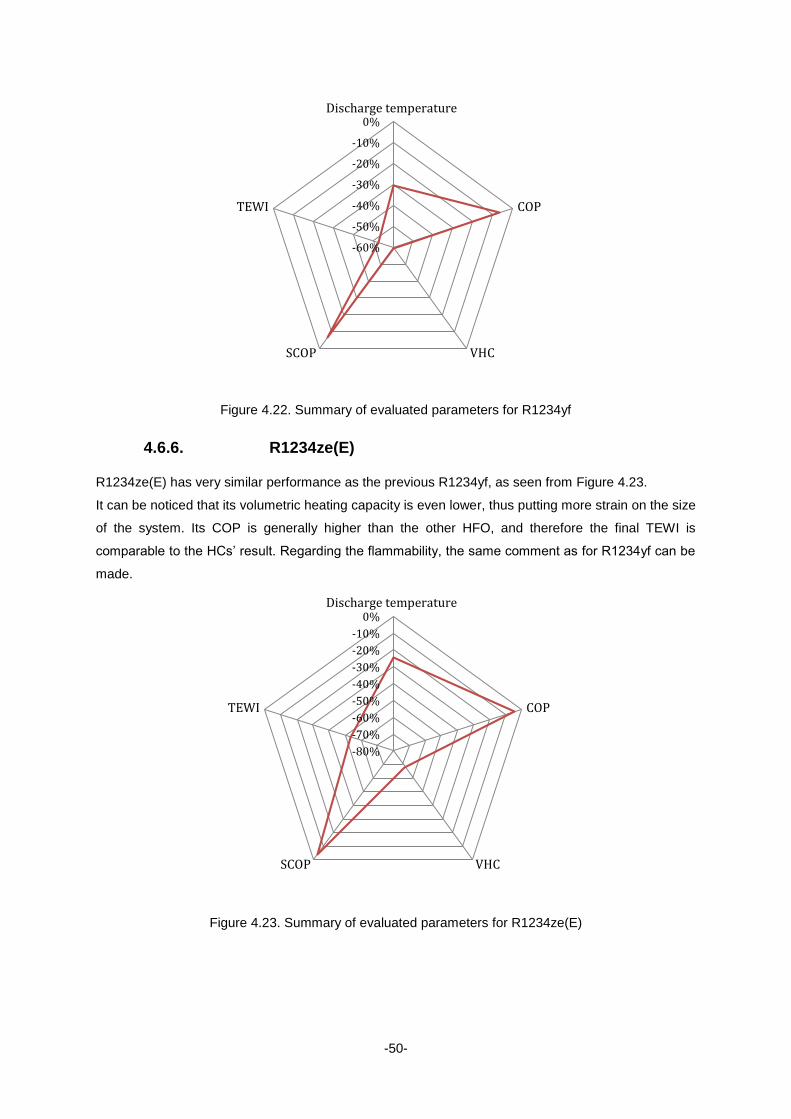
-50-

Figure 4.22. Summary of evaluated parameters for R1234yf

4.6.6. R1234ze(E)

R1234ze(E) has very similar performance as the previous R1234yf, as seen from Figure 4.23.

It can be noticed that its volumetric heating capacity is even lower, thus putting more strain on the size

of the system. Its COP is generally higher than the other HFO, and therefore the final TEWI is

comparable to the HCs’ result. Regarding the flammability, the same comment as for R1234yf can be

made.

Figure 4.23. Summary of evaluated parameters for R1234ze(E)

-60%

-50%

-40%

-30%

-20%

-10%


COP

VHCSCOP

TEWI

-80%

-70%

-60%

-50%

-40%

-30%

-20%

-10%


COP

VHCSCOP

TEWI

-51-

5. Conclusions and further work

As a result of the F-gas regulation implemented in 2015, the refrigeration industry has to move towards

the reduction of its contribution to the emissions of fluorinated gases, as they have a non neglectable

role in the global warming. To contribute to this effort, this work investigates possibile alternatives to

R410A, currently in usage in commerically avaliable heat pump, typically used in a single house in

Sweden. Eight options were identified, six of which were analysed in the model created, namely R32,

R152a, R290, R1270, R1234yf and R1234ze(E). The study of the remaining two, i.e. R450A and

R513A, is postponed to a second phase, as the data available was no sufficient to perform a valid

comparison.

The most relevant results considered in the scope of this study were obtained for both radiator and floor

types of heating systems and consist of:

- the VHC, in the temperature range -22 °C to 16 °C

- the COP of the heat pump, in the temperature range -22 °C to 16 °C

- the discharge temperature, in the temperature range -22 °C to 16 °C

- the SCOP, for the overall heating season

- the TEWI factor

It is important to understand that the results obtained are highly dependent on the area for which they

have been calculated, namely Sweden – colder climate scenario, and low CO2 emission factor of the

national energy mix. Therefore, the conclusion drawn from this study are only valid in the mentioned

specific climatic characteristics.

The performance of the heat pump with the alternative refrigerants, as seen through the COP, was

variable. At the lowest temperatures, R410A presents a lower COP than R32, R152a and both the HCs

(up to -7 °C). With the increasing outdoor temperature, the baseline performance improves but remains

poorer than R32 along the whole temperature range (8.19% and 7.72% relative difference respectively

at -22 °C and 16 °C). The worst COPs were shown by the HFOs.

The overall highest SCOP was thus given by R32 (+6.46% for radiator, +6.77% for floor heating),

outperforming R410A in both radiator and floor heating cases. R152a also presented positive outcome,

having a higher SCOP than R410A in radiator heating case (+2.28%), and an almost identical one in

the floor heating case (-0.089%). The other options entailed lower seasonal performances, with the

worst result obtained by the HFOs (and in particular R1234yf with -6.4%).

When evaluating the overall environmental impact of the refrigerants, through TEWI a general reduction

of CO2 equivalent emissions is calculated. Whereas the indirect effect is similar for every option

considered – slightly increasing with decreasing SCOP – the direct effect is drastically reduced with the

decrease of the GWP. In fact, both the HCs and the HFOs obtain a remarkable reduction of the TEWI

factor (in order for R290, R1270, R1234ze(E) and R1234yf: -54.6%, -54.2%, -53.7%, -52.5%), in

accordance to their extremely low GWP. The lowest emissions’ reduction is obtained by R32 (-40.8%),

which, in spite of an improved performance in the machine, still has a considerable GWP.

-52-

Moreover, the reaching by R32 of discharge temperatures above the safety limit cannot be neglected,

as it could endanger the compressor’s functioning. On the other hand, this drawback could be mitigated

by the use of a smaller refrigerant charge. In fact, R32 presents a higher VHC when compared to R410A

(+12.4%). The other evaluated options all present a lower one, with the biggest reduction owned by the

HFOs.

The interpretation of these results and the selection of a most favourable option is then closely related

with the direction that the manufacturer wants to take. If the preference is to keep a certain heating

capacity, R32 offers the possibility of using smaller charge and thus smaller systems. This way, the final

result in the TEWI evaluation would be a further reduction, due to a smaller direct effect. Furthermore,

if the aim is to reduce the CO2 as much as possible, the HFOs and the HCs represent a better option

in a country with a high share of renewable, clean energies and thus a small CO2 emission factor.

It is also paramount to keep into consideration the different flammability levels of the refrigerants. None

of the options evaluated in this study are non-flammable, and thus they all require some restrictions in

their use, e.g. charge limitations, location of the installation restrictions. HCs are the most subject to

limitations, as they belong to the A3 – high flammability – category. R32, R1234yf and R1234ze(E)

belong to the A2L category. As of today, regulations do not differentiate between A2L and A2 levels.

This situation could be modified in the near future, representing an advantage for these three

refrigerants, as it would mean less strict limitations in use.

In this concern, the two remaining options that could not be evaluated at this stage – R450A and R513A

– present the advantage over the other refrigerants as they are not flammable.

In order to further this Thesis’ work, future steps will aim at integrating the two refrigerants that were left

out in this first phase, i.e. R450A and R513A, and at improving the existing model.

Specifically, the first task can easily be performed once valid compressor’s models exist for the the two

refrigerants; in order for the results to be included in the presented report and compared with the other

alternatives, the correlation for the compressor needs to be obtained in the same way as for all studied

fluids. This information was not available at this time.

Secondly, a few aspects can be treated in order to enhance the model created. In particular, the UAs

model can be improved by elaborating correlations from a wider range of experimental data. Moreover,

some of the compressor’s isentropic efficiency correlations (R32 and R1234ze(E)) were not available,

and thus had to be assumed by similarity with other refrigerants. With more precise information, more

accurate efficiencies in these two cases can be integrated.

Lastly, detailed recommendations can be elaborated with deeper knowledge of the preferences of the

manufacturing company. Combining them with the restrictions imposed by the Standard EN378, an

accurate set of operating conditions to be respected, and consequently an improved calculation of the

CO2 emissions’ reduction, can be provided.

-53-

Bibliography

AIRAH. 2012. Methods of calculating Total Equivalent Warming Impact (TEWI) 2012. s.l. : The

Australian Institute of Refrigeration, Air conditioning and Heating, 2012.

Andres, R. J., Boden, T. a., Bréon, F. M., Ciais, P., Davis S., Erickson, D., Treanton, K. 2012. A

synthesis of carbon dioxide emissions from fossil-fuel combustion. s.l. : Biogeosciences, 2012.

AREA. 2014. AREA F-Gas Guide. s.l. : AREA, 2014.

Balmer, Robert T. 2011. Modern engineering thermodynamic. s.l. : Academic press, 2011.

Barve, Atharva. 2010. Study of low global warming potential refrigerants in heat pump systems for

stationary applications. 2010.

Bathkar, V.W. 2013. Alternative refrigerants in vapour compression refrigeration cycle for sustainable

environment: a review of recent research. s.l. : Islamic Azad University, 2013.

Bitzer. 2014. New EU F-Gas regulation . s.l. : Bitzer, 2014.

—. 2014. Refrigerant report 18. s.l. : Bitzer, 2014.

BSI. 2012. Air conditioners, liquid chilling packages and heat pumps, with electrically driven

compressors, for space heating and cooling — Testing and rating at part load conditions and calculation

of seasonal performance. s.l. : BSI Standards Publication, 2012.

Calm, James M. 2008. The next generation of refrigerants – Historical review, considerations and

outlook. Great Falls : International Journal of Refrigeration, 2008.

Convenant of Mayors. 2012. The emission factors. 2012.

Daikin Global . 2014. CSR Report. s.l. : Daikin Global, 2014.

Danfoss. 2014. Refrigerant options now and in the future. s.l. : Danfoss, 2014.

—. 2011. Why compressors fail. Part 4 - overheating . s.l. : Danfoss, 2011.

DuPont. 2015. Understanding the Refrigerant "R" Nomenclature. DuPont . [Online] 2015. [Cited: 10 02

2015.] http://www2.dupont.com/Refrigerants/en_CA/products/understanding.html.

ehpa. 2014. European Heat Pump Market and Statistics Report | Soon Available. ehpa. [Online] 08 10

2014. [Cited: 20 06 2015.] http://www.ehpa.org/about/news/article/european-heat-pump-market-and-

statistics-report-soon-available/.

Ekroth, I., Granryd, E. 2011. The vapor compression cycle. [book auth.] Erik Granryd et al.

Refrigerating engineering. Stockholm : Department of Energy Technology, KTH, 2011.

Emerson climate technologies. 2015. Select Online. Emerson climate technologies. [Online] 2015.

[Cited: 15 02 2015.] http://selectonline.emersonclimate.eu/SelectOnline/.

Environmental Protection Agency. 2015. Ozone Layer Protection - Alternatives / SNAP.

Environmental Protection Agency. [Online] 2015. [Cited: 17 03 2015.] http://www.epa.gov/ozone/snap/.

European Commission . 2014. Fluorinated Greenhouse gases. European Commission. [Online] 11

12 2014. [Cited: 11 02 2015.] http://ec.europa.eu/clima/policies/f-gas/index_en.htm.

Eurostat. 2015. Renewable energy statistics. Eurostat - statistics explained. [Online] 05 08 2015.

[Cited: 15 08 2015.] http://ec.europa.eu/eurostat/statistics-

explained/index.php/Renewable_energy_statistics#Primary_production.

Forsén, Martin. 2005. Heat pumps - Technology and environmental impact. s.l. : ehpa, 2005.

Global Greenhouse Warming. 2015. Global Warming Potential. Global Greenhouse Warming.

[Online] 2015. [Cited: 10 02 2015.] http://www.global-greenhouse-warming.com/global-warming-

potential.html.

-54-

Gluckman consulting. 2014. EU F-Gas Regulation Guidance - Information Sheet 26: Bans for New

Products and Equipment. s.l. : Gluckman consulting, 2014.

Hakkaki-Fard, Ali. 2014. Applying refrigerant mixtures with thermal glide in cold climate air-source heat

pumps. s.l. : Applied thermal engineering, 2014.

Ho-Saeng Leea, Hyeon-Ju Kima, Dong-gyu Kangb, Dongsoo Jung. 2012. Thermodynamic

performance of R32/R152a mixture for water source heat pumps. s.l. : Energy, 2012.

Industrial Heat Pumps. 2015. Coefficient of Performance. Industrial Heat Pumps. [Online] 2015.

[Cited: 11 02 2015.]

Institut International du Froid. 2011. Classification of refrigerants . Paris : Institut International du

Froid, 2011.

IPCC. 2005. Ozone depletion potentials (ODPs) and equivalent effective stratospheric chlorine (EESC).

Safeguarding the Ozone Layer and the Global Climate System: Issues Related to Hydrofluorocarbons

and Perfluorocarbons (SROC). s.l. : Cambridge University Press, 2005.

Itten, R., Frischknecht, R., Stucki, M. 2012. Life Cycle Inventories of Electrici-ty Mixes and Grid. Uster

(Switzerland) : Paul Scherrer Institute, 2012. 229.

Ken Schultz, Steve Kujak. 2013. System Drop-In Tests of R134a Alternative Refrigerants (ARM-42a,

N-13a, N-13b, R-1234ze(E), and OpteonTM XP10) in a 230-RT Water-Cooled Water Chiller. s.l. : AHRI,

2013.

Ki-Jung Park, Dongsoo Jung. 2009. Performance of heat pumps charged with R170/R290 mixture.

s.l. : Applied Energy, 2009.

Linde . 2015. Industrial Gases. The Linde group. [Online] Linde, 2015. [Cited: 08 06 2015.]

http://www.linde-

gas.com/en/products_and_supply/refrigerants/natural_refrigerants/R1270_propylene/index.html.

Linde. 2015. HFOs. Linde - Industrial Gases. [Online] 2015. [Cited: 13 02 2015.] http://www.linde-

gas.com/en/products_and_supply/refrigerants/HFO_refrigerants/solstice_1234ze/index.html.

—. 2015. R717 (Ammonia). Linde - Industrial gases. [Online] 2015. [Cited: 12 02 2015.]

http://www.linde-

gas.com/en/products_and_supply/refrigerants/natural_refrigerants/R717_ammonia/index.html.

—. 2015. R744 (Carbon Dioxide). Linde - Industrial gases. [Online] 2015. [Cited: 12 02 2015.]

http://www.linde-

gas.com/en/products_and_supply/refrigerants/natural_refrigerants/R744_carbon_dioxide/index.html.

Martin Forsen, Peter Roots, Anne-Lee Bertenstam. 2008. Market status for ground source heat

pumps in Europe. s.l. : GroundReach, 2008.

Maul, Joachin. 2013. Environment-friendly heating with R290 heat pumps . 2013.

McLinden, Mark O. 2014. A thermodynamic analysis of refrigerants: Possibilities and tradeoffs for Low-

GWP refrigerants. s.l. : International Journal of Refrigeration, 2014.

Mohanraj, M. 2011. A review on recent developments in new refrigerant mixtures for vapour

compression-based refrigeration,air-conditioning and heat pump units. Calicut : International Journal of

Energy Research, 2011.

—. 2011. A review on recent developments in new refrigerant mixtures for vapour compression-based

refrigeration,air-conditioning and heat pump units. Calicut : International Journal of Energy Research,

2011.

Mota-Babiloni, Adrian. 2014. Drop-in energy performance evaluation of R1234yf and R1234ze(E) in

a vapor compression system as R134a replacements. s.l. : Applied thermal engineering, 2014.

—. 2014. Experimental study of an R1234ze(E)/R134a mixture (R450A) as R134a replacement. s.l. :

International journal of refrigeration, 2014.

-55-

Rothlin, Peter. 2011. Refrigerants. [book auth.] Erik Granryd et al. Refrigerating engineering.

Stockholm : Department of energy technology, KTH, 2011.

Sarbu, Ioan. 2014. A review on substitution strategy of non-ecological refrigerants from vapour

compression-based refrigeration, air-conditioning and heat pump systems. s.l. : International Journal of

Refrigeration, 2014.

SWEP International AB. 2012. Glide refrigerants. SWEP - A Dover company. [Online] 2012. [Cited:

11 02 2015.] http://handbooks.swep.net/RefrigerantHandbook/chapter_06/Pages/6.4-Glide-

Refrigerants.aspx.

Transparency market research. 2015. Geothermal Heat Pumps Market to be Driven by the Rising Oil

Prices. Transparency Market Research. [Online] 08 05 2015. [Cited: 20 06 2015.]

http://www.transparencymarketresearch.com/pressrelease/geothermal-heat-pumps-market.htm.

United Nations Environment Programme - Ozone Secreteriat . 2011. List of Parties categorized as

operating under Article 5 paragraph 1 of the Montreal Protocol (considered as developing countries).

United Nations Environment Programme - Ozone Secreteriat . [Online] 2011. [Cited: 17 03 2015.]

http://ozone.unep.org/new_site/en/parties_under_article5_para1.php.

Xiaowei Fan, Xianping Zhang, Fengkun Wang. 2013. Simulation Study on a Heat Pump System

Using R744/R290 as refrigerant. s.l. : Journal of Civil Engineering and Architecture, 2013.

Zhang, Shengjun. 2014. Evaluation of non-azeotropic mixtures containing HFOs as potential

refrigerants in refrigeration and high-temperature heat pump systems. s.l. : Science China, 2014.

-i-

Appendix - EES code -

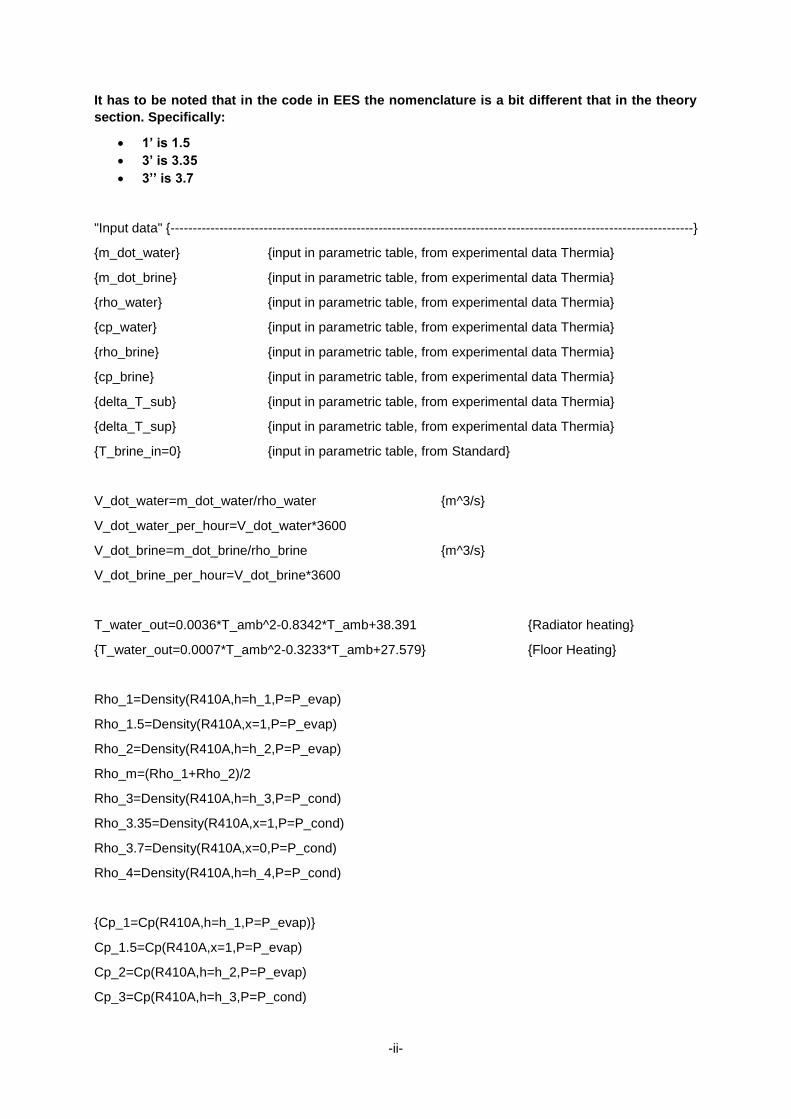
-ii-

It has to be noted that in the code in EES the nomenclature is a bit different that in the theory

section. Specifically:

1’ is 1.5

3’ is 3.35

3’’ is 3.7

"Input data" {----------------------------------------------------------------------------------------------------------------------}

{m_dot_water} {input in parametric table, from experimental data Thermia}

{m_dot_brine} {input in parametric table, from experimental data Thermia}

{rho_water} {input in parametric table, from experimental data Thermia}

{cp_water} {input in parametric table, from experimental data Thermia}

{rho_brine} {input in parametric table, from experimental data Thermia}

{cp_brine} {input in parametric table, from experimental data Thermia}

{delta_T_sub} {input in parametric table, from experimental data Thermia}

{delta_T_sup} {input in parametric table, from experimental data Thermia}

{T_brine_in=0} {input in parametric table, from Standard}

V_dot_water=m_dot_water/rho_water {m^3/s}

V_dot_water_per_hour=V_dot_water*3600

V_dot_brine=m_dot_brine/rho_brine {m^3/s}

V_dot_brine_per_hour=V_dot_brine*3600

T_water_out=0.0036*T_amb^2-0.8342*T_amb+38.391 {Radiator heating}

{T_water_out=0.0007*T_amb^2-0.3233*T_amb+27.579} {Floor Heating}

Rho_1=Density(R410A,h=h_1,P=P_evap)

Rho_1.5=Density(R410A,x=1,P=P_evap)

Rho_2=Density(R410A,h=h_2,P=P_evap)

Rho_m=(Rho_1+Rho_2)/2

Rho_3=Density(R410A,h=h_3,P=P_cond)

Rho_3.35=Density(R410A,x=1,P=P_cond)

Rho_3.7=Density(R410A,x=0,P=P_cond)

Rho_4=Density(R410A,h=h_4,P=P_cond)

{Cp_1=Cp(R410A,h=h_1,P=P_evap)}

Cp_1.5=Cp(R410A,x=1,P=P_evap)

Cp_2=Cp(R410A,h=h_2,P=P_evap)

Cp_3=Cp(R410A,h=h_3,P=P_cond)

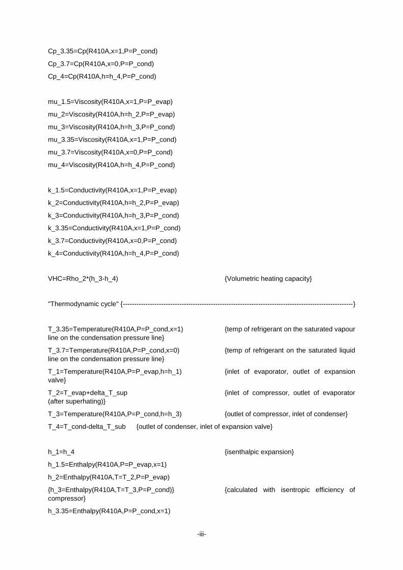
-iii-

Cp_3.35=Cp(R410A,x=1,P=P_cond)

Cp_3.7=Cp(R410A,x=0,P=P_cond)

Cp_4=Cp(R410A,h=h_4,P=P_cond)

mu_1.5=Viscosity(R410A,x=1,P=P_evap)

mu_2=Viscosity(R410A,h=h_2,P=P_evap)

mu_3=Viscosity(R410A,h=h_3,P=P_cond)

mu_3.35=Viscosity(R410A,x=1,P=P_cond)

mu_3.7=Viscosity(R410A,x=0,P=P_cond)

mu_4=Viscosity(R410A,h=h_4,P=P_cond)

k_1.5=Conductivity(R410A,x=1,P=P_evap)

k_2=Conductivity(R410A,h=h_2,P=P_evap)

k_3=Conductivity(R410A,h=h_3,P=P_cond)

k_3.35=Conductivity(R410A,x=1,P=P_cond)

k_3.7=Conductivity(R410A,x=0,P=P_cond)

k_4=Conductivity(R410A,h=h_4,P=P_cond)

VHC=Rho_2*(h_3-h_4) {Volumetric heating capacity}

"Thermodynamic cycle" {------------------------------------------------------------------------------------------------------}

T_3.35=Temperature(R410A,P=P_cond,x=1) {temp of refrigerant on the saturated vapour

line on the condensation pressure line}

T_3.7=Temperature(R410A,P=P_cond,x=0) {temp of refrigerant on the saturated liquid

line on the condensation pressure line}

T_1=Temperature(R410A,P=P_evap,h=h_1) {inlet of evaporator, outlet of expansion

valve}

T_2=T_evap+delta_T_sup {inlet of compressor, outlet of evaporator

(after superhating)}

T_3=Temperature(R410A,P=P_cond,h=h_3) {outlet of compressor, inlet of condenser}

T_4=T_cond-delta_T_sub {outlet of condenser, inlet of expansion valve}

h_1=h_4 {isenthalpic expansion}

h_1.5=Enthalpy(R410A,P=P_evap,x=1)

h_2=Enthalpy(R410A,T=T_2,P=P_evap)

{h_3=Enthalpy(R410A,T=T_3,P=P_cond)} {calculated with isentropic efficiency of

compressor}

h_3.35=Enthalpy(R410A,P=P_cond,x=1)

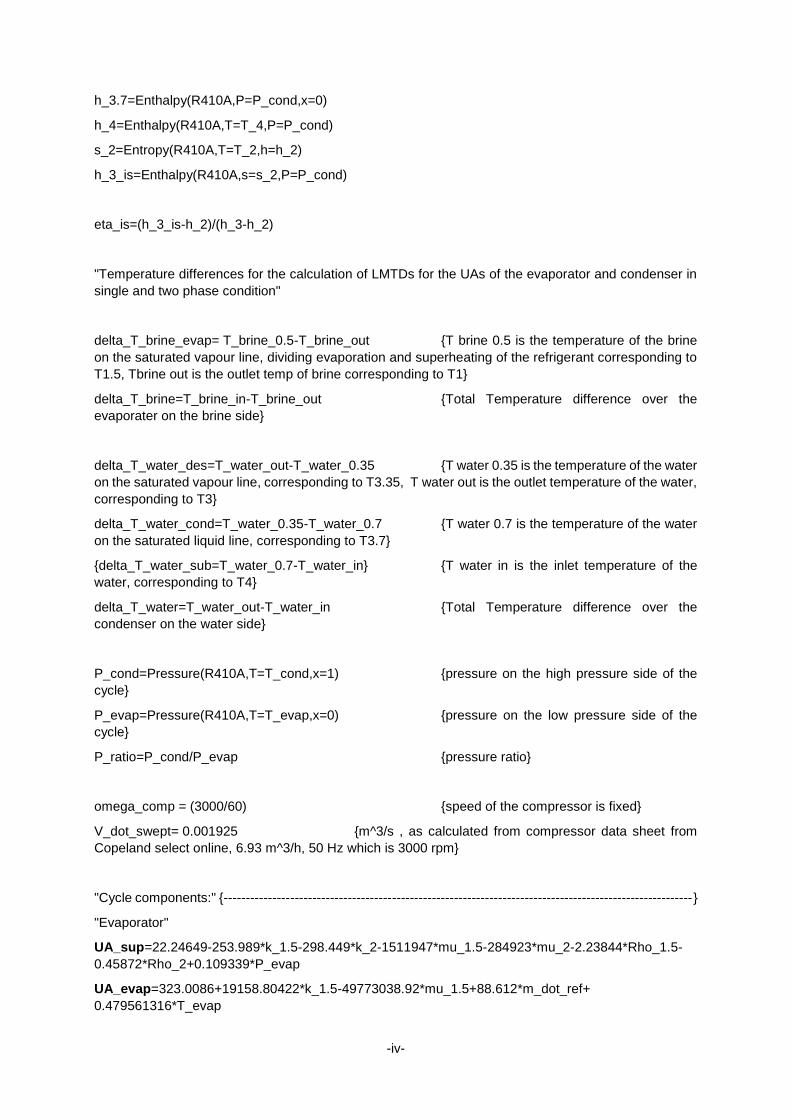
-iv-

h_3.7=Enthalpy(R410A,P=P_cond,x=0)

h_4=Enthalpy(R410A,T=T_4,P=P_cond)

s_2=Entropy(R410A,T=T_2,h=h_2)

h_3_is=Enthalpy(R410A,s=s_2,P=P_cond)

eta_is=(h_3_is-h_2)/(h_3-h_2)

"Temperature differences for the calculation of LMTDs for the UAs of the evaporator and condenser in

single and two phase condition"

delta_T_brine_evap= T_brine_0.5-T_brine_out {T brine 0.5 is the temperature of the brine

on the saturated vapour line, dividing evaporation and superheating of the refrigerant corresponding to

T1.5, Tbrine out is the outlet temp of brine corresponding to T1}

delta_T_brine=T_brine_in-T_brine_out {Total Temperature difference over the

evaporater on the brine side}

delta_T_water_des=T_water_out-T_water_0.35 {T water 0.35 is the temperature of the water

on the saturated vapour line, corresponding to T3.35, T water out is the outlet temperature of the water,

corresponding to T3}

delta_T_water_cond=T_water_0.35-T_water_0.7 {T water 0.7 is the temperature of the water

on the saturated liquid line, corresponding to T3.7}

{delta_T_water_sub=T_water_0.7-T_water_in} {T water in is the inlet temperature of the

water, corresponding to T4}

delta_T_water=T_water_out-T_water_in {Total Temperature difference over the

condenser on the water side}

P_cond=Pressure(R410A,T=T_cond,x=1) {pressure on the high pressure side of the

cycle}

P_evap=Pressure(R410A,T=T_evap,x=0) {pressure on the low pressure side of the

cycle}

P_ratio=P_cond/P_evap {pressure ratio}

omega_comp = (3000/60) {speed of the compressor is fixed}

V_dot_swept= 0.001925 {m^3/s , as calculated from compressor data sheet from

Copeland select online, 6.93 m^3/h, 50 Hz which is 3000 rpm}

"Cycle components:" {----------------------------------------------------------------------------------------------------------}

"Evaporator"

UA_sup=22.24649-253.989*k_1.5-298.449*k_2-1511947*mu_1.5-284923*mu_2-2.23844*Rho_1.5-

0.45872*Rho_2+0.109339*P_evap

UA_evap=323.0086+19158.80422*k_1.5-49773038.92*mu_1.5+88.612*m_dot_ref+

0.479561316*T_evap

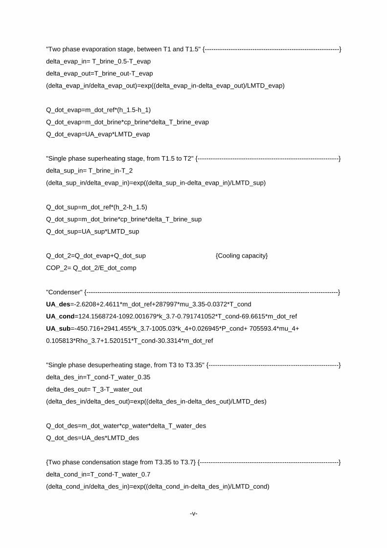
-v-

"Two phase evaporation stage, between T1 and T1.5" {--------------------------------------------------------------}

delta_evap_in= T_brine_0.5-T_evap

delta_evap_out=T_brine_out-T_evap

(delta_evap_in/delta_evap_out)=exp((delta_evap_in-delta_evap_out)/LMTD_evap)

Q_dot_evap=m_dot_ref*(h_1.5-h_1)

Q_dot_evap=m_dot_brine*cp_brine*delta_T_brine_evap

Q_dot_evap=UA_evap*LMTD_evap

"Single phase superheating stage, from T1.5 to T2" {-----------------------------------------------------------------}

delta_sup_in= T_brine_in-T_2

(delta_sup_in/delta_evap_in)=exp((delta_sup_in-delta_evap_in)/LMTD_sup)

Q_dot_sup=m_dot_ref*(h_2-h_1.5)

Q_dot_sup=m_dot_brine*cp_brine*delta_T_brine_sup

Q_dot_sup=UA_sup*LMTD_sup

Q_dot_2=Q_dot_evap+Q_dot_sup {Cooling capacity}

COP_2= Q_dot_2/E_dot_comp

"Condenser" {--------------------------------------------------------------------------------------------------------------------}

UA_des=-2.6208+2.4611*m_dot_ref+287997*mu_3.35-0.0372*T_cond

UA_cond=124.1568724-1092.001679*k_3.7-0.791741052*T_cond-69.6615*m_dot_ref

UA_sub=-450.716+2941.455*k_3.7-1005.03*k_4+0.026945*P_cond+ 705593.4*mu_4+

0.105813*Rho_3.7+1.520151*T_cond-30.3314*m_dot_ref

"Single phase desuperheating stage, from T3 to T3.35" {------------------------------------------------------------}

delta_des_in=T_cond-T_water_0.35

delta_des_out= T_3-T_water_out

(delta_des_in/delta_des_out)=exp((delta_des_in-delta_des_out)/LMTD_des)

Q_dot_des=m_dot_water*cp_water*delta_T_water_des

Q_dot_des=UA_des*LMTD_des

{Two phase condensation stage from T3.35 to T3.7} {----------------------------------------------------------------}

delta_cond_in=T_cond-T_water_0.7

(delta_cond_in/delta_des_in)=exp((delta_cond_in-delta_des_in)/LMTD_cond)

-vi-

Q_dot_cond=m_dot_ref*(h_3.35-h_3.7)

Q_dot_cond=m_dot_water*cp_water*delta_T_water_cond

Q_dot_cond=UA_cond*LMTD_cond

{Single phase subcooling stage from T3.7 to T4} {---------------------------------------------------------------------}

delta_sub_in=T_4-T_water_in

(delta_sub_in/delta_cond_in)=exp((delta_sub_in-delta_cond_in)/LMTD_sub)

Q_dot_sub=m_dot_ref*(h_3.7-h_4)

Q_dot_sub=m_dot_water*cp_water*delta_T_water_sub

Q_dot_sub=UA_sub*LMTD_sub

Q_dot_1=Q_dot_des+Q_dot_cond+Q_dot_sub {heating capacity}

COP_1=Q_dot_1/E_dot_comp

"Compressor" {------------------------------------------------------------------------------------------------------------------- }

eta_is=0.0024*P_ratio^3-0.0363*P_ratio^2+0.1377*P_ratio+0.5531

eta_s=0.0015*P_ratio^2-0.0356*P_ratio+1.0583

rho_ref_2=Density(R410A,h=h_2,P=P_evap) {density of refrigerant at inlet of compressor}

m_dot_ref=rho_ref_2*V_dot_swept*eta_s

E_dot_comp=m_dot_ref*(h_3-h_2) {Total power input to the compressor}

delta_P=((m_dot_ref/0.00018727)^2)/(2*Rho_1)*((1-1.4829^2+(0.42*(1-1.4289^2)^2))+

4*1.2028*(Rho_1/Rho_m)+2*(Rho_1/Rho_2-1)-((1-0.51074^2-(1-0.51074)^2)*(Rho_1/Rho_2)))

"SCOP calculation" {----------------------------------------------------------------------------------------------- ------------}

heating_season_tot= 6446

COP_partial=COP_1*hj/heating_season_tot

SCOP=SumParametric('SCOP_Rad','COP_partial')

SCOP=SumParametric('SCOP_Floor','COP_partial')

Documents

Next generation of refrigerants for residential heat pump ...Next generation of refrigerants for residential heat pump systems Martina Longhini ... as thermodynamic characteristics