Newton's law of heating and the heat equation

INVOLVE 2:4(2009)

Newton’s law of heating and the heat equationMark Gockenbach and Kristin Schmidtke

(Communicated by Suzanne Lenhart)

Newton’s law of heating models the average temperature in an object by a simpleordinary differential equation, while the heat equation is a partial differentialequation that models the temperature as a function of both space and time. Aseries solution of the heat equation, in the case of a spherical body, shows thatNewton’s law gives an accurate approximation to the average temperature if thebody is not too large and it conducts heat much faster than it gains heat from thesurroundings. Finite element simulation confirms and extends the analysis.

1. Introduction

A popular application involving an elementary differential equation is Newton’slaw of heating, which describes the change in temperature in an object whose sur-roundings are hotter than it is.1 If the temperature at time t is T (t), then Newton’slaw of heating is

T ′ = α(Ts − T ), T (0)= T0, (1)

where Ts and T0 are constants representing the temperature of the surroundingsand the initial temperature of the object, respectively.2 The differential equationin (1) simply states that the rate of change of the temperature is proportional tothe difference between the temperatures of the surroundings and the object. Thesolution of (1) is

T (t)= Ts − (Ts − T0)e−αt . (2)

MSC2000: 35K05.Keywords: heat equation, Newton’s law of heating, finite elements, Bessel functions.

1If the surroundings are colder, then the differential equation is called Newton’s law of cooling.For definiteness of language, we will usually assume that heating is occurring.

2We take T0 and Ts to be constants, as this agrees with the usual textbook presentation of New-ton’s law of heating, which we wish to analyze in this paper. There is nothing that would preventus from allowing Ts to depend on time, or T0 to depend on space (so that T0(x, y, z) is the initialtemperature at the point (x, y, z) in the object). If T0 were variable, then we would use the averagevalue T 0 of T0 in the ordinary differential equation model (1) and the variable T0 itself in the partialdifferential equation model presented below. Allowing nonconstant T0 and/or Ts would considerablycomplicate the analysis in this paper.

419

420 MARK GOCKENBACH AND KRISTIN SCHMIDTKE

Newton’s law of heating is included in virtually every introductory textbook ondifferential equations, such as [Boyce and DiPrima 1992; Zill 2005].

Newton’s law of heating assumes that the temperature of the object is repre-sented by a single number. A more sophisticated model represents the object asoccupying a domain � in R3 and its temperature as a function u(x, y, z, t), where(x, y, z) ∈�. The governing partial differential equation is the heat equation

ρc∂u∂t= κ1u in �, t > 0. (3)

In this equation, 1u is the Laplacian of u:

1u =∂2u∂x2 +

∂2u∂y2 +

∂2u∂z2 .

The quantities ρ, c, and κ describe the material properties of the object; ρ is thedensity, c is the specific heat, and κ is the thermal conductivity. Typically, κ isgiven in J/s cm K, ρ in g/cm3, and c in J/g K. For a derivation of the heat equation,the reader can consult introductory books on partial differential equations, such as[Gockenbach 2002; Haberman 2004].

To obtain a complete description of u, we must model how � exchanges heatenergy with its surroundings. We adopt a model much like Newton’s law of heating:

κ∂u∂n= α(Ts − u) on ∂�. (4)

This is called a Robin boundary condition; it states that the heat flux across theboundary is proportional to the difference between Ts and the temperature on ∂�.Although the form of the boundary condition is analogous to Newton’s law ofheating, there is no reason to expect that the constants α and α are the same;indeed, since they have different units, it would be surprising if their numericalvalues were the same.

The PDE (3) and the boundary condition (4), together with an initial condition,form a well-posed problem that determines u uniquely. We assume that the ini-tial temperature in � is constant and obtain the following initial boundary valueproblem (IBVP):

ρc∂u∂t− κ1u = 0 in �, t > 0,

u(x, y, z, 0)= T0 in �,

κ∂u∂n+αu = αTs on ∂�, t > 0.

(5)

We now have two models to describe the temperature of the given object, namely,Newton’s law of heating and the heat equation together with a Robin boundary

NEWTON’S LAW OF HEATING AND THE HEAT EQUATION 421

condition. The simpler model (1) would be an adequate substitute for the morecomplicated model (5) if T is close to the average temperature in � as predictedby (5):

u =1|�|

∫�

u. (6)

Before we can compare the solutions T and u, we must determine the relativevalues of the constants α and α appearing in (1) and (5), respectively. Fortunately,given α, the value of α is suggested by the following calculation:

dudt=

1|�|

∫�

∂u∂t=

1ρc|�|

∫�

ρc∂u∂t=

1ρc|�|

∫�

κ1u

=1

ρc|�|

∫∂�

κ∂u∂n=

1ρc|�|

∫∂�

α(Ts − u).

If we define ub = ub(t) to be the average value of u on ∂�,

ub =1|∂�|

∫∂�

u,

then ∫∂�

α(Ts − u)= α|∂�|(Ts − ub),

and we obtain

u′ =α|∂�|

ρc|�|(Ts − ub). (7)

We then see that u satisfies a differential equation similar to Newton’s law of heat-ing, but with α replaced with

α =|∂�|

ρc|�|α. (8)

Of course, even with this value of α, (1) and (7) are not the same, since (7) showsthat the rate of change of u is determined not by u itself, but by ub. However, theequations are similar enough that we might expect T to be a good approximationto u.

The primary purpose of this paper is to compare the solutions of the heat equa-tion (5) and Newton’s law of heating (1), where α is given by (8). We will use bothanalytical and numerical methods; to make the analysis tractable and the numericssimpler, we will assume that the object is spherical.


2. Solution of the heat equation on a spherical domain

We will henceforth assume that � is the ball of radius R centered at the origin.Since the initial value of u is a constant and the boundary conditions are con-stant on ∂�, the solution to the IBVP (5) depends only on the radial variabler =

√x2+ y2+ z2. This follows from the fact that the Laplacian 1 is invariant

under any rotation of the coordinate system (for a nice discussion of this, the readercan consult [Folland 1995, Section 2.A]). We can therefore write u = u(r, t), andwe recall that

1u =∂2u∂r2 +

2r∂u∂r

(see, for example, [Haberman 2004]). The IBVP (5) can thus be rewritten as

ρc∂u∂t− κ

(∂2u∂r2 +

2r∂u∂r

)= 0, 0< r < R, t > 0,

u(r, 0)= T0, 0< r < R,

κ∂u∂r(R, t)+αu(R, t)= αTs, t > 0.

(9)

In addition to the equations explicitly listed above, there is the implicit requirementthat u be finite at r =0. We use the technique of shifting the data to transform (9) toa problem with homogeneous boundary conditions. We define Y (r)= ar2, wherea is chosen so that Y satisfies the boundary condition κY ′(R)+αY (R)= αTs ,

a =αTs

2κR+αR2 , (10)

and write u(r, t)=U (r, t)+ Y (r). Then U satisfies

ρc∂U∂t− κ

(∂2U∂r2 +

2r∂U∂r

)= 6aκ, 0< r < R, t > 0,

U (r, 0)= T0− ar2, 0< r < R,

κ∂U∂r(R, t)+αU (R, t)= 0, t > 0.

(11)

We can derive a solution to (11) by expanding U in terms of the eigenfunctionsof the spatial operator

L =−κ(

d2

dr2 +2r

ddr

),

where homogeneous Robin conditions are imposed on the eigenfunctions:

κv′(R)+αv(R)= 0. (12)


We will now briefly derive these eigenfunctions and the corresponding eigenvalues.First, using integration by parts, we can show that if v1, v2 satisfy (12), then∫ R

0−κ

(d2v1

dr2 +2r

dv1

dr

)v2(r)r2 dr = αv1(R)v2(R)R2

+

∫ R

0κ

dv1

drdv2

drr2 dr.

This shows that L is symmetric with respect to the inner product

〈v1, v2〉 =

∫ r

0v1(r)v2(r)r2 dr,

that is, that 〈L(v1), v2〉 = 〈v1, L(v2)〉 for all v1, v2 satisfying the given boundaryconditions. The standard argument then shows that the eigenvalues of L are all real,and that eigenfunctions of L corresponding to distinct eigenvalues are orthogonalwith respect to the given inner product [Gockenbach 2002, Section 5.1]. We alsosee that

〈L(v), v〉 = αv(R)2+∫ R

0κ

(dvdr(r))2

r2 dr,

which is positive for every nonzero function v. This implies that all the eigenvaluesof L are positive.

We now wish to solve

−κ

(d2v

dr2 +2r

dvdr

)= λv, 0< r < R,

κv′(R)+αv(R)= 0,(13)

for λ > 0 and v = v(r). It is well known [Arfken and Weber 2005] that the onlysolutions to (13)1 that are bounded at the origin are multiples of

j0(√λ/κ r

),

where j0 is the first spherical Bessel function:

j0(s)=sin (s)

s.

(For more information about Bessel functions, including the properties cited below,the reader can consult [Trantor 1968] or the comprehensive reference [?].) Theproblem of finding the eigenvalues and eigenfunctions then reduces to finding thevalues of λ>0 such that v(r)= j0

(√λ/κ r

)satisfies the boundary condition (13)2.

Substituting v into (13)2 and simplifying yields

tan (s)= ms, m =κ

κ −αR, s = R

√λ/κ. (14)


We will henceforth make the important assumption that κ−αR>0 or, equivalently,that

β =αRκ< 1. (15)

Recalling that κ is the thermal conductivity within the object and α describes howwell thermal energy is transmitted to the environment, this assumption means thatthe object conducts energy more quickly than it transmits energy to the surround-ings and also that the radius of the object is not too large. Our intuition ought totell us that these are precisely the conditions under which Newton’s law of heatingshould give accurate results. In fact, below we will expand u(t)− T (t) in powersof β and show that u(t)− T (t)= O(β) uniformly for t ≥ 0.

Assumption (15) implies that m = 1/(1− β) > 1 in (14), and a simple graphthen shows that (14) has positive solutions s1, s2, s3, . . . , with

(k− 1)π < sk <(

k−12

)π, k = 1, 2, 3, . . .

and sk ≈(k− 1

2

)π for k≥ 2. For our analysis below, we need accurate estimates of

the sk’s. To estimate s1, we can expand tan (s) in powers of s, truncate the series,and obtain

s1 =√

3β1/2−

√3

10β3/2+ O(β5/2),

λ1 =3κR2

(β − 1

5β2+ O(β3)

).

(16)

For k ≥ 2, we see that each sk is greater than the corresponding solution sk totan (s) = s. We write sk =

(k− 1

2

)π − εk , expand tan

((k− 1

2

)π − εk

)in powers

of εk , and solve to get

sk ≥ sk =(k−

12

)π

(1−

1(k− 1

2

)2π2−

2

3(k− 1

2

)4π4+ . . .

). (17)

In particular, we find that

0.95(k− 1

2

)π < sk <

(k− 1

2

)π, k = 2, 3, . . . . (18)

This estimate will suffice for our purposes below.We now write

vk(r)= j0(√λk/κ r

)=

sin(√λk/κ r

)√λk/κ r

, k = 1, 2, 3, . . . , (19)

for the eigenfunctions of L . The standard theory of (spherical) Bessel functionsguarantees that any function u=u(r) (finite at the origin) can be expanded in terms


of the orthogonal functions v1, v2, v3, . . . . We can therefore expand the solutionU of (11) as

U (r, t)=∞∑

k=1

Ck(t)vk(r).

Substituting this expression into the PDE (11)1 yields∞∑

k=1

{ρcC ′k(t)+ λkCk(t)

}vk(r)=

∞∑k=1

bkvk(r),

where∑∞

k=1 bkvk(r) is the expansion of the constant function 6aκ:

bk =6aκ

∫ R0 vk(r)r2 dr∫ R

0 vk(r)2r2 dr, k = 1, 2, 3, . . . . (20)

From the initial condition (11)2, we have∞∑

k=1

Ck(0)vk(r)=∞∑

k=1

dkvk(r),

where∑∞

k=1 dkvk(r) is the expansion of T0− ar2:

dk =

∫ R0 (T0− ar2)vk(r)r2 dr∫ R

0 vk(r)2r2 dr, k = 1, 2, 3, . . . . (21)

We then obtain the following initial value problem for Ck :

ρcC ′k + λkCk = bk, Ck(0)= dk, k = 1, 2, 3, . . . .

The solution is

Ck(t)=bk

λk+

(dk −

bk

λk

)e−λk t/(ρc), k = 1, 2, 3, . . . . (22)

We now have the following solution to the IBVP (9):

u(r, t)= ar2+

∞∑k=1

Ck(t)vk(r). (23)

The reader will recall that

u =1|�|

∫�

u.

With � equal to the ball of radius R, this reduces to

u(t)=4π

(4/3)πR3

∫ R

0u(r, t)r2 dr =

3R3

∫ R

0u(r, t)r2 dr,


and so

u(t)=3R3

∫ R

0ar4 dr +

∞∑k=1

{3R3

∫ R

0vk(r)r2 dr

}Ck(t) (24)

(since the solution u to the heat equation is known to be smooth, the series for ucan be integrated term-by-term to produce (24)).

3. Comparing the solutions

We now have formulas for both T (t) and u(t), and we wish to bound |T (t)−u(t)|for t ≥ 0. Since vk is oscillatory for k ≥ 2 (see Figure 1 and also the definition ofvk in (19)), we expect

3R3

∫ R

0vk(r)r2 dr

to be small for k ≥ 2. We hypothesize, then, that u(t) will be well approximatedby

u1(t)=3R3

∫ R

0ar4 dr +

(3R3

∫ R

0v1(r)r2 dr

)C1(t).

We therefore wish to show that |T (t)−u1(t)| and |u1(t)−u(t)| are both small fort ≥ 0.

A straightforward calculation shows that

3R3

∫ R

0vk(r)r2 dr = 3

sin(R√λk/κ

)− R√λk/κ cos

(R√λk/κ

)(R√λk/κ

)3 ,

0 1

1

Figure 1. The first five eigenfunctions v1, v2, v3, v4, v5 on the in-terval [0, R], R = 1.0. To construct this graph, we have takenκ = 1.0 and α = 0.001. The first eigenfunction is nearly constanton the interval [0, R], while, for k ≥ 2, vk is increasingly oscilla-tory as k increases.


or3R3

∫ R

0vk(r)r2 dr = 3

sin (sk)− sk cos (sk)

s3k

.

Since tan (sk)= msk , or sk cos sk = m−1 sin sk , we obtain

3R3

∫ R

0vk(r)r2 dr = 3

m− 1m

sin sk

s3k

= 3βsin sk

s3k

. (25)

For k ≥ 2, we can apply (18) to obtain∣∣∣∣ 3R3

∫ R

0vk(r)r2 dr

∣∣∣∣≤ 3βs3

k

≤3β

(0.95 (k− 1/2) π)3,

which yields ∣∣∣∣ 3R3

∫ R

0vk(r)r2 dr

∣∣∣∣≤ 1

8 (k− 1/2)3β, k = 2, 3, . . . . (26)

For k = 1, we expand the integral in powers of β, which is a straightforwardcalculation:3

3R3

∫ R

0v1(r)r2 dr = 1−

310β + O

(β2) . (27)

The results given in (25) and (27) support our hypothesis that u(t) should be wellapproximated by u1(t).

We can now complete the bound |T (t)−u1(t)| in short order. From (16)2, (20),and (21), we find that

b1

λ1= Ts + O

(β2)

and

d1−b1

λ1= T0− Ts +

310(T0− Ts)β + O

(β2) . (28)

We can also expand the constant term in the series for u(t) in powers of β:

3R3

∫ R

0ar4 dr =

3a R2

5=

3Ts

10β + O

(β2) .

Putting these results together, we obtain

u1(t)= Ts − (Ts − T0)e−λ1t/(ρc)+ O

(β2) . (29)

The reader should notice how the O(β) term has canceled (compare the productof (27) and (28)). The only dependence of the O

(β2)

term on t is through theexponential (this dependence is not shown explicitly here), which is bounded by

3We used Mathematica to generate this and other series expansions.


one for t ≥ 0. Thus the O(β2)

term is uniformly small for t ≥ 0 (assuming β issmall).

The similarity between T (t) and u1(t) is now obvious (compare (2) and (29)).It remains only to compare the exponentials e−λ1t/(ρc) and e−αt

= e−3αt/(ρcR). Wehave

λ1 =3κR2β

(1−

15β + O(β2)

)=

3αR

(1−

15β + O(β2)

)(30)

(using β = αR/κ), so we see that λ1/(ρc) and α = 3α/(ρcR) are quite similar,with

e−λ1t/(ρc)≥ e−αt , t ≥ 0.

To obtain a useful bound, we maximize the function

f (t)= e−λ1t/(ρc)− e−αt , t ≥ 0.

The function f has a unique stationary point, and we easily obtain

0≤ e−λ1t/(ρc)− e−αt

≤15eβ + O

(β2) , t ≥ 0. (31)

We can now bound the difference between T (t) and u1(t):

|T (t)− u1(t)| =∣∣Ts − (Ts − T0)e−αt

− Ts + (Ts − T0)e−λ1t/(ρc)+ O(β2)

∣∣=∣∣(Ts − T0)(e−λ1t/(ρc)

− e−αt)∣∣+ O(β2)

≤|Ts − T0|

5eβ + O(β2).

As noted above, this bound is uniform over the interval 0≤ t <∞.Finally, we bound |u1(t)− u(t)| for t ≥ 0. We will merely sketch the results,

which the interested reader can verify. We already have the upper bound (26) for∣∣∣∣ 3R3

∫ R

0vk(r)r2 dr

∣∣∣∣ .We will need upper bounds for dk and bk/λk , which will require a lower bound for∫ R

0vk(r)2r2 dr.

A straightforward calculation gives∫ R

0vk(r)2r2 dr =

κ

λk

(R2−

sin(2√λk/κ R

)4√λk/κ

)≥

R3

4 (k− 1/2)2 π2(32)

(applying the upper bound for λk implied by (18)). We then have

bk =6aκ

∫ R0 vk(r)r2 dr∫ R

0 vk(r)2r2 dr,


and (26) gives an upper bound for the numerator. Applying this upper bound to-gether with (32) and simplifying yields

bk ≤3κTsπ

2

2R5(k− 1

2

)β2.

Since (18) implies

λk ≥ 0.952(k− 12

)2π2κ, k = 2, 3, . . . , (33)

we obtain (after a little manipulation)

bk

λk≤

2Ts

R5(k− 1

2

)3β2. (34)

Obtaining a bound for dk is more work. We have∫ R

0(T0− ar2)vk(r)r2 dr

=κ

(2+β)λ5/2k R2

·{−

√λk R

(6βκTs + λk R2((2+β)T0−βTs)

)cos (

√λk/κ R)

+√κ(6βκTs + λk R2((2+β)T0− 3βTs)

)sin (

√λk/κ R)

}=

κ3/2

(2+β)λ5/2k R2

·{(sin sk − sk cos sk)

(6βκTs + λk R2((2+β)T0−βTs)

)− 2βT2 sin sk

}.

Since sin sk = msk cos sk , we have

sin sk − sk cos sk = (m− 1)sk cos sk =β

1−βsk cos sk .

Also, sk is an approximate root of cosine; using (17) and the Taylor expansion ofcosine around s = (k− 1/2) π , we obtain sk cos sk = O(1). Using this and somemore manipulation, we find positive constants γ1 and γ2 such that∣∣∣∣∫ R

0(T0− ar2)vk(r)r2 dr

∣∣∣∣≤ γ1β + γ2β2

λ3/2k

, k = 2, 3, . . . .

This, together with the lower bound (32), yields

dk =

∫ R0 (T0− ar2)vk(r)r2 dr∫ R

0 vk(r)2r2 dr≤ γ1β + γ2β

2, (35)

where γ1 and γ2 are positive constants.


We can finally use (26), (34), and (35) to bound |u1(t)− u(t)|. We have

|u1(t)− u(t)| ≤∞∑

k=2

(3R3

∫ R

0vk(r)r2 dr

)∣∣∣bk

λk+

(dk −

bk

λk

)e−λk t/(ρc)

∣∣∣≤

∞∑k=2

β

8(k− 1/2)3

(2∣∣∣bk

λk

∣∣∣+ |dk |

).

Since∞∑

k=2

1(k− 1

2

)3

is finite, (34) and (35) yield positive constants γ1 and γ2 such that

|u1(t)− u(t)| ≤ γ1β2+ γ2β

3, t ≥ 0.

This, together with our earlier bound on |T (t)− u1(t)|, yields our final result:

|T (t)− u(t)| ≤|Ts − T0|

5eβ + O(β2), t ≥ 0. (36)

The reader will recall that

β =αRκ,

where κ is the thermal conductivity with the object, α describes how well the objecttransmits heat energy to its surroundings (or vice versa), and R is the radius of �.As long as α� κ and � is not too large, (36) shows that the average temperaturein � will be well approximated by Newton’s law of heating.

4. The finite element method

We wish to give some numerical examples to illustrate the above analysis. Thisrequires that we be able to compute accurate solutions to the initial-boundary valueproblem (9). We will use the standard Galerkin–Crank–Nicolson finite elementmethod, which we now briefly describe.

To compute the solution of (9), we first rewrite the problem in its variationalform:∫ R

0ρc∂u∂t(r, t)v(r)r2 dr +

∫ R

0κ∂u∂r(r, t)v′(r)r2 dr +αR2u(R, t)v(R)

= αR2Tsv(R), for all v ∈ V . (37)

Here V is the space of test functions,

V ={v ∈ H 1(0, R) : rv ∈ L2(0, R), rv′ ∈ L2(0, R)

},


based on the Sobolev space H 1(0, R) (the space of functions with one square-integrable (weak) derivative). The variational form (37) results from multiplyingthe PDE (9) by a test function, integrating over �, integrating the ∂2u/∂r2 term byparts, and applying the boundary condition. It is well known that the variationalform is equivalent to the original initial-boundary value problem (at least when, asin this case, the original problem is known to have a smooth solution).

We obtain the semidiscrete form of (37) by discretizing in space using piecewiselinear functions on a mesh defined by ri = ih, h = R/n, and applying Galerkin’smethod. We will write Vh for the space of continuous piecewise linear functionson the given mesh, and {φ0, φ1, . . . , φn} for the usual nodal basis defined by

φi (r j )=

{1 if i = j,0 if i 6= j.

The semidiscrete solution is

uh(r, t)=n∑

j=0

α j (t)φ j (r),

satisfying∫ R

0ρc∂uh

∂t(r, t)v(r)r2 dr +

∫ R

0κ∂uh

∂r(r, t)v′(r)r2 dr +αR2uh(R, t)v(R)

= αR2Tsv(R), for all v ∈ Vh . (38)

Choosing v = φi , i = 0, 1, . . . , n, (38) is equivalent to

Ma′+ (K +G)a = F, (39)

where M and K are the mass and stiffness4 matrices,

Mi j =

∫ R

0ρcφ j (r)φi (r)r2 dr, Ki j =

∫ R

0κφ′j (r)φ

′

i (r)r2 dr, i, j = 0, 1, . . . , n.

Every entry in the matrix G is zero except the n, n entry, and similarly only then-th component of the vector F is nonzero:

Gnn = αR2, Fn = αR2Ts .

This scheme is O(h2) in the sense that there is a constant C > 0 (depending on thetrue solution u) such that

‖u(·, t)− uh(·, t)‖ ≤ Ch2 for all t ≥ 0,

4The terminology comes from mechanics, the discipline that popularized finite element methods.


where

‖u(·, t)− uh(·, t)‖ =[∫ R

0(u(r, t)− uh(r, t))2r2 dr

]1/2

.

To obtain a fully discrete scheme, (39) is discretized in time by the Crank–Nicolson method,

M(a(k+1)

− a(k)

1t

)+ (K +G)

(a(k+1)+ a(k)

2

)= F,

to obtain (M +

1t2

B)

a(k+1)=

(M −

1t2

B)

a(k)+1t F, (40)

where a(k) is the approximation to a(tk), tk = k1t , k = 0, 1, 2, . . . .We write u(k)(r) for the approximation to uh(r, tk) obtained by estimating a(tk)

by a(k). Then there exists constants C1,C2 > 0 such that, for all k,

‖u(·, tk)− u(k)‖ ≤ C1h2+C21t2.

This error bound (and the earlier bound on the error in the semidiscrete solution)can be obtain by a straightforward generalization of the standard error analysisfound in Thomee [2006].

5. Examples

We will now show several examples, demonstrating the effectiveness of the aboveanalysis. In these examples, we compare the solution (2) of Newton’s law of heat-ing with an accurate solution of the heat equation computed by the finite elementmethod described above.

Example 1 (A small iron ball). We first consider an iron ball approximately thesize of a baseball: R = 3.7 cm. The physical constants describing iron are c =0.437 J/g K, ρ = 7.88 g/cm3, and κ = 0.802 J/s cm. Various references suggestvalues of α (the convection heat transfer coefficient in air) from 10−2 to 10−3

W/cm2K; we will use a value of α = 0.0045. The corresponding value of α is

α =3αρcR≈ 0.0010596.

We assume that the initial temperature of the ball is T0 = 0◦ C and that thetemperature of the surrounding air is Ts = 25◦ C, and simulate the temperaturein the ball for one hour. The average temperature u computed by solving theheat equation and the temperature T predicted by Newton’s law of heating areindistinguishable on a graph (see Figure 2); the maximum difference between thetwo is about 0.038187.


500 1000 1500 2000 2500 3000 3500

5

10

15

20

25

500 1000 1500 2000 2500 3000 3500

0.01

0.02

0.03

Figure 2. Left: The average temperature of the iron ball in Exam-ple 1. Right: The difference u(t)−T (t) between the temperaturescalculated from the heat equation and Newton’s law of heating. Inboth graphs, the horizontal axis is time in seconds, and the verticalis degrees Celsius.

In this example, we have β = αRκ≈ 0.020761, and the first-order bound on the

error is|Ts − T0|

5eβ ≈ 0.038107.

With a small value of β, the analysis suggests that Newton’s law is an accuratesubstitute for the heat equation, and that conclusion is confirmed by the numericalresults. Moreover, the first-order bound on the difference between the two solutionsis an excellent estimate of the actual difference.

Example 2 (A large iron ball). The second example is the same as the first, exceptnow the radius of the ball is R = 100 cm. The value of β is now approximately0.56110, so we do not expect that Newton’s law will yield a particularly accurateestimate of the true average temperature. We simulate the temperature for 20 hours(since it takes a long time to appreciably change the temperature in such a largeball).

As Figure 3 shows, the maximum difference between the two solutions is about0.97333. The first-order bound on the error is

|Ts − T0|

5eβ ≈ 1.0321.

Once again, the analysis proves to be quite accurate.

Example 3 (A small styrofoam ball). In the last example, Newton’s law of heating,while not a bad approximation, did not accurately model the average temperaturein the ball because the ball was so large. In this example, we consider the otherreason why Newton’s law might not work particularly well, namely, that heat flowsslowly through the object compared to how quickly it flows from the surroundingsto the object. We consider a styrofoam ball of radius R = 3.7 cm. The physical


10 000 20 000 30 000 40 000 50 000 60 000 70 000

5

10

15

20

10 000 20 000 30 000 40 000 50 000 60 000 70 000

0.2

0.4

0.6

0.8

1.0

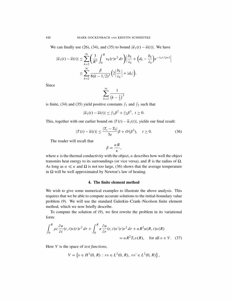
Figure 3. Left: The temperatures of the iron ball in Example 2,as predicted by the heat equation and Newton’s law of heating.(The larger temperature is predicted by Newton’s law.) Right: Thedifference u(t)− T (t) between the temperatures calculated fromthe heat equation and Newton’s law.

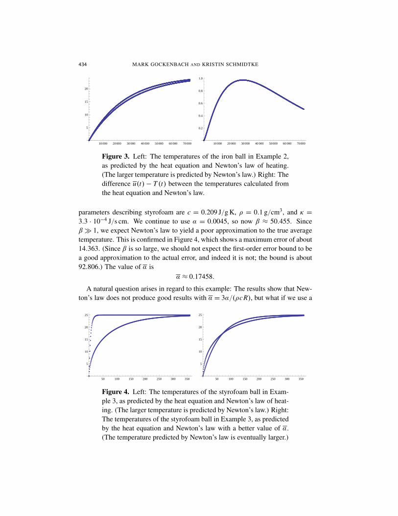
parameters describing styrofoam are c = 0.209 J/g K, ρ = 0.1 g/cm3, and κ =3.3 · 10−4 J/s cm. We continue to use α = 0.0045, so now β ≈ 50.455. Sinceβ� 1, we expect Newton’s law to yield a poor approximation to the true averagetemperature. This is confirmed in Figure 4, which shows a maximum error of about14.363. (Since β is so large, we should not expect the first-order error bound to bea good approximation to the actual error, and indeed it is not; the bound is about92.806.) The value of α is

α ≈ 0.17458.

A natural question arises in regard to this example: The results show that New-ton’s law does not produce good results with α = 3α/(ρcR), but what if we use a

50 100 150 200 250 300 350

5

10

15

20

25

50 100 150 200 250 300 350

5

10

15

20

25

Figure 4. Left: The temperatures of the styrofoam ball in Exam-ple 3, as predicted by the heat equation and Newton’s law of heat-ing. (The larger temperature is predicted by Newton’s law.) Right:The temperatures of the styrofoam ball in Example 3, as predictedby the heat equation and Newton’s law with a better value of α.(The temperature predicted by Newton’s law is eventually larger.)


different value of α? To answer this question, we found the value of α that producesa solution (2) as close as possible to u in the least-squares sense; that is, we foundα to minimize

J (α)=N∑

k=1

(u(tk)− Ts + (Ts − T0)e−αtk )2

(where N is the number of time steps in the finite element simulation). We denotethe optimal value of α by α; the result in this example is

α ≈ 0.016805.

With this value of α, Newton’s law yields a much improved estimate of the averagetemperature of the ball. Nevertheless, the result is still not very good (see Figure 4),which shows that, for this example, the true average temperature in the styrofoamball is simply not well modeled by Newton’s law of heating.

6. Concluding remarks

Our results show that for a small spherical object with the property that heat flowsthrough the object more quickly than it flows to the surroundings (β =αR/κ� 1),Newton’s law of heating provides a satisfactory model of the average temperatureof the object. Moreover, the value

α =3αρcR

is a satisfactory constant of proportionality in Newton’s law. To carry out thisanalysis, we have assumed that the initial temperature of the object is constantthroughout, and also that the temperature of the surroundings is held constant.

The alert reader may have noticed that the analysis suggests an even better valueof α. The estimate of λ1 in (30) suggests that

α =3αρcR

(1−

15β)

would be an improved estimate of λ1/(ρc) and hence lead to a better estimate ofu by T . Indeed, the reader can easily check that this value of α leads to an O(β2)

bound for |u(t)− T (t)|, t ≥ 0.Many textbook problems on Newton’s law of cooling refer to inhomogeneous

objects; perhaps the classic example is the cooling of a cup of coffee; see, forexample, [Boyce and DiPrima 1992, Section 2.5, problem 14]. (Another popularexample is the cooling of a corpse!) Nothing in our analysis allows us to addresseither inhomogeneities in the object or complex geometries. However, we canapply finite element simulation to an inhomogeneous sphere. For example, wecan consider a hollow styrofoam ball filled with water, the closest we can get to


200 400 600 800 1000 1200

20

40

60

80

100

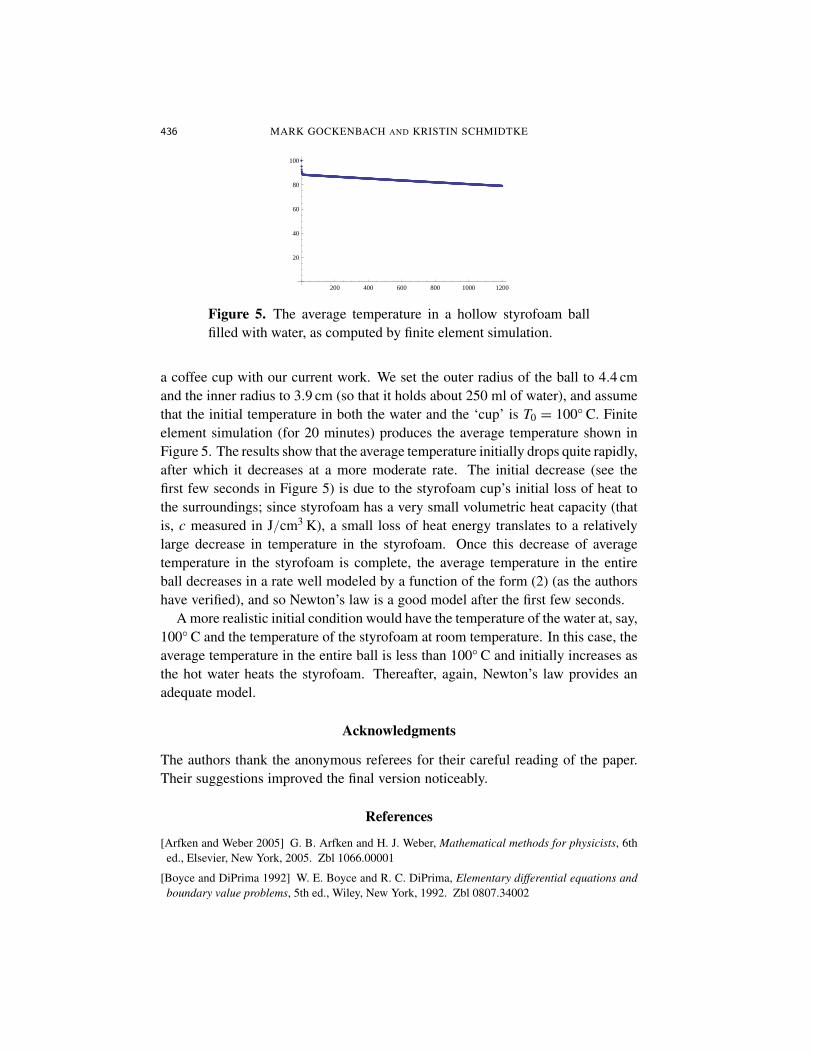
Figure 5. The average temperature in a hollow styrofoam ballfilled with water, as computed by finite element simulation.

a coffee cup with our current work. We set the outer radius of the ball to 4.4 cmand the inner radius to 3.9 cm (so that it holds about 250 ml of water), and assumethat the initial temperature in both the water and the ‘cup’ is T0 = 100◦ C. Finiteelement simulation (for 20 minutes) produces the average temperature shown inFigure 5. The results show that the average temperature initially drops quite rapidly,after which it decreases at a more moderate rate. The initial decrease (see thefirst few seconds in Figure 5) is due to the styrofoam cup’s initial loss of heat tothe surroundings; since styrofoam has a very small volumetric heat capacity (thatis, c measured in J/cm3 K), a small loss of heat energy translates to a relativelylarge decrease in temperature in the styrofoam. Once this decrease of averagetemperature in the styrofoam is complete, the average temperature in the entireball decreases in a rate well modeled by a function of the form (2) (as the authorshave verified), and so Newton’s law is a good model after the first few seconds.

A more realistic initial condition would have the temperature of the water at, say,100◦ C and the temperature of the styrofoam at room temperature. In this case, theaverage temperature in the entire ball is less than 100◦ C and initially increases asthe hot water heats the styrofoam. Thereafter, again, Newton’s law provides anadequate model.

Acknowledgments

The authors thank the anonymous referees for their careful reading of the paper.Their suggestions improved the final version noticeably.

References

[Arfken and Weber 2005] G. B. Arfken and H. J. Weber, Mathematical methods for physicists, 6thed., Elsevier, New York, 2005. Zbl 1066.00001

[Boyce and DiPrima 1992] W. E. Boyce and R. C. DiPrima, Elementary differential equations andboundary value problems, 5th ed., Wiley, New York, 1992. Zbl 0807.34002


[Folland 1995] G. B. Folland, Introduction to partial differential equations, 2nd ed., Princeton Uni-versity Press, Princeton, NJ, 1995. MR 96h:35001 Zbl 0841.35001

[Gockenbach 2002] M. S. Gockenbach, Partial differential equations: analytical and numericalmethods, Soc. Ind. Appl. Math., Philadelphia, 2002. MR 2003m:35001

[Haberman 2004] R. Haberman, Applied partial differential equations with fourier series and bound-ary value problems, 4th ed., Prentice Hall, Upper Saddle River, NJ, 2004.

[Thomée 2006] V. Thomée, Galerkin finite element methods for parabolic problems, 2nd ed., Seriesin Computational Math. 25, Springer, Berlin, 2006. MR 2007b:65003 Zbl 1105.65102

[Trantor 1968] C. J. Trantor, Bessel functions with some physical applications, Hart, New York,1968.

[Watson 1944] G. N. Watson, A treatise on the theory of Bessel functions, 2nd ed., CambridgeUniversity Press, Cambridge, 1944. Reprinted 1995. MR 96i:33010 Zbl 0849.33001

[Zill 2005] D. G. Zill, A first course in differential equations, 8th ed., Brooks/Cole, Belmont, 2005.Zbl 0785.34002

Received: 2008-11-25 Revised: 2009-06-15 Accepted: 2009-07-13

[email protected] Department of Mathematical Sciences,Michigan Technological University, 1400 Townsend Drive,Houghton, MI 49931-1295, United States

[email protected] Department of Mathematical Sciences,Michigan Technological University, 1400 Townsend Drive,Houghton, MI 49931-1295, United States

Documents

Newton's law of heating and the heat equation