1

Newtonian Model of an Elite Sprinter: How Much Force do Athletes

Need to Produce Each Step to be World Class?

Jeremy Richmond

BSc-Physics, MExSpSc (candidate University of Sydney)

Fitness First Randwick Australia

ABSTRACT

A model is presented of the force and power produced during a world record sprint to provide

coaches and athletes with a method to determine how much force to use during strength

training and what velocity to train at. In addition to specific velocity of strength training, the

coach or athlete can estimate the biomechanical position of the athlete by determining that

position for the relevant step so that training can be specific to the movement pattern of actual

sprinting. The model is determined by using empirical data to develop relationships between

the variables of time, velocity, instantaneous velocity, contact time and distance travelled over

each individual step. The formula used for the Newtonian model is applied to an athlete,

Matic Osovnikar, and shows weakness in the strength of one particular leg above a certain

velocity during steps 6, 8 and 10. The lack of force produced by that leg results in negative

velocity of the athlete during steps 8 and 10. From the comparison of data from Matic

Osovnikar with the Newtonian model, a suggestion is for the athlete to undertake velocity

specific and movement specific strength training of that leg to improve performance during

steps 6, 8 and 10. This may improve the overall sprint performance for the athlete.

Key words: Force, velocity, contact time

Introduction

The 100-m sprint is, according to Summers (1997), the most exciting of Olympic events and

the winner is often referred to as the “world’s fastest human”. In order to accelerate to

maximum velocity it is crucial to have speed, strength, or power (Tricoli et al. 2005) with

power being the product of speed (velocity) and strength (force). An understanding of the

influence of force and velocity on sprinting is needed to critique the effectiveness of current

training methods such as high resistance, Olympic lifting, power, over-speed, ballistics,

plyometric training and resisted running. Such a critique is necessary as a number of

researchers have found that these methods provide little significant benefit to sprinting

(Delecluse et al.1995, Rimmer & Sleivert 2000, Majdell & Alexander 1991, McBride et al.

2002, Kristensen et al.2006, Spinks et al.2007, Wilson et al. 1993, Gorostiaga 2003, Lyttle et

al. 1996, Hoffman et al., Kotzaminidis et al. 2005, Tricoli et al. 2005, Harris et al. 2000),

especially when compared to sprint training itself. Perhaps these exercise methods are not

specific enough to sprinting to provide reasonable transfer of strength gains (Young 1992)

and may need to be modified to specifically target the muscles relevant for sprinting, so as to

have more significance.

Even when different exercises involve identical muscle groups the specific movement pattern

used in training is where most strength improvement will occur (Weiss 1991). Furthermore,

the greatest strength gains will occur at or near the training velocity (Behm & Sale 1993).

According to Rutherford & Jones (1986) the movement pattern specificity in strength training

probably enhances the role of learning and coordination. Almasbakk & Hoff (1996) agree

that the development of coordination is the determining factor in early velocity specific

strength. Sale (1992) points out that improved coordination may be the result of the most

2

efficient activation of the muscles involved, and the most efficient activation of motor units

within each muscle.

Logic would suggest that for improved coordination in sprinting, practice of sprinting itself

would be sufficient. This argument does have weight in light of the fact that, as mentioned

previously, training methods have proven little over and above sprint training itself. However,

the limitation of sprint training alone is that at top speed an athlete does not have a facility to

overload and improve further. In addition, the biomechanical position adopted during the

initial acceleration phase cannot be maintained sufficiently for enough steps to allow

reasonable practice required to produce an improvement to learning and coordination of

muscle activation. Exercises need to be created which mimic the force, velocity, and

movement patterns in order to allow an athlete to improve their sprinting skill.

The effect of sprint training itself was accounted for by Delecluse et al. (1995) who compared

heavy resistance and sprint training with plyometric and sprint training, and with sprint

training alone. They found that the plyometric and sprint training group experienced

significant improvement compared to the other groups for acceleration over 10m, improved in

maximum velocity and was the only group to improve 100m times. Similarly, Rimmer and

Slievert (2000) compared sprint training to plyometric training exclusively and found an

improvement in time over 10m for the plyometric training group who did not undertake any

sprint training. This suggests that velocity specific training methods can benefit sprinting,

although the magnitude of any benefit seems to be limited to small gains within the first 10m.

The downfall of traditional strength training methods in terms of improvements to sprint

performance may be a lack of velocity specificity to actual sprinting but they may also lack

sufficient movement specificity.

Strength training methods with more velocity specificity may have better influence on sprint

performance. Blazevich and Jenkins (2002) tested the effects of a high resistance low velocity

training protocol and a low resistance high velocity training protocol on sprinters who were

concurrently sprint and plyometric training. Although the result was not significant, the high

velocity low resistance group improved more in sprint acceleration. However, no account was

made for the effects of sprint training alone or for the effects of the plyometric protocols that

the sprinters were participating in at the time. The strength training exercises used in the

training protocol including hip extension and hip flexion seemed to mimic the movements in

actual sprinting, which may have facilitated a reasonable transfer of strength gains.

The enhancement of sprint performance through the combined effects of strength and

plyometric protocols has not been proven (Lyttle et al. 1996, Tricoli et al. 2005). Heavy

resistance combined with explosive movement in the jump squat exercise has been found to

be detrimental to sprint performance (McBride et al. 2002), although the use of lighter more

optimal resistance in the same exercise has shown small acceleration benefits. Wilson et al.

(1993) found that optimal (maximal) power jump squat training produced better sprint results

over 30m than protocols involving squat resistance training and plyometric depth jump

training. However the positive effects of this protocol compared to the benefit of sprint

training alone is yet to be validated. Nevertheless a more specific optimal power training

derivative of the jump squat may be more effective for sprinting if the movement pattern of

actual sprinting beyond that of the start can be replicated.

For the design of any sprint training program, knowledge of the fundamental biomechanical

factors is critical to performance (Mero et al. 1992). Some researchers believe that faster top

running speeds are achieved with greater ground forces (Weyand et al. 2000). More

specifically, Young et al. (1995) found strong correlations between maximum sprinting speed

and the force (relative to bodyweight) applied at 100ms from the start of a concentric loaded

jump (r=0.80, p=0.0001), the countermovement jump (r=-0.79) and maximum force during a

jump takeoff (r=-0.79). These results show a strong correlation between sprint performance

and maximum force applied in a force production time frame specific to sprinting, and the

3

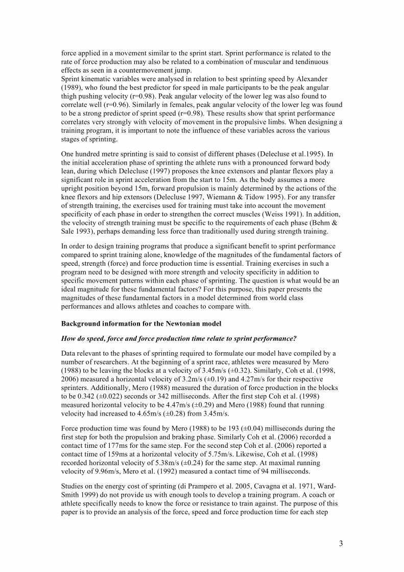
force applied in a movement similar to the sprint start. Sprint performance is related to the

rate of force production may also be related to a combination of muscular and tendinuous

effects as seen in a countermovement jump.

Sprint kinematic variables were analysed in relation to best sprinting speed by Alexander

(1989), who found the best predictor for speed in male participants to be the peak angular

thigh pushing velocity (r=0.98). Peak angular velocity of the lower leg was also found to

correlate well (r=0.96). Similarly in females, peak angular velocity of the lower leg was found

to be a strong predictor of sprint speed (r=0.98). These results show that sprint performance

correlates very strongly with velocity of movement in the propulsive limbs. When designing a

training program, it is important to note the influence of these variables across the various

stages of sprinting.

One hundred metre sprinting is said to consist of different phases (Delecluse et al.1995). In

the initial acceleration phase of sprinting the athlete runs with a pronounced forward body

lean, during which Delecluse (1997) proposes the knee extensors and plantar flexors play a

significant role in sprint acceleration from the start to 15m. As the body assumes a more

upright position beyond 15m, forward propulsion is mainly determined by the actions of the

knee flexors and hip extensors (Delecluse 1997, Wiemann & Tidow 1995). For any transfer

of strength training, the exercises used for training must take into account the movement

specificity of each phase in order to strengthen the correct muscles (Weiss 1991). In addition,

the velocity of strength training must be specific to the requirements of each phase (Behm &

Sale 1993), perhaps demanding less force than traditionally used during strength training.

In order to design training programs that produce a significant benefit to sprint performance

compared to sprint training alone, knowledge of the magnitudes of the fundamental factors of

speed, strength (force) and force production time is essential. Training exercises in such a

program need to be designed with more strength and velocity specificity in addition to

specific movement patterns within each phase of sprinting. The question is what would be an

ideal magnitude for these fundamental factors? For this purpose, this paper presents the

magnitudes of these fundamental factors in a model determined from world class

performances and allows athletes and coaches to compare with.

Background information for the Newtonian model

How do speed, force and force production time relate to sprint performance?

Data relevant to the phases of sprinting required to formulate our model have compiled by a

number of researchers. At the beginning of a sprint race, athletes were measured by Mero

(1988) to be leaving the blocks at a velocity of 3.45m/s (±0.32). Similarly, Coh et al. (1998,

2006) measured a horizontal velocity of 3.2m/s (±0.19) and 4.27m/s for their respective

sprinters. Additionally, Mero (1988) measured the duration of force production in the blocks

to be 0.342 (±0.022) seconds or 342 milliseconds. After the first step Coh et al. (1998)

measured horizontal velocity to be 4.47m/s (±0.29) and Mero (1988) found that running

velocity had increased to 4.65m/s (±0.28) from 3.45m/s.

Force production time was found by Mero (1988) to be 193 (±0.04) milliseconds during the

first step for both the propulsion and braking phase. Similarly Coh et al. (2006) recorded a

contact time of 177ms for the same step. For the second step Coh et al. (2006) reported a

contact time of 159ms at a horizontal velocity of 5.75m/s. Likewise, Coh et al. (1998)

recorded horizontal velocity of 5.38m/s (±0.24) for the same step. At maximal running

velocity of 9.96m/s, Mero et al. (1992) measured a contact time of 94 milliseconds.

Studies on the energy cost of sprinting (di Prampero et al. 2005, Cavagna et al. 1971, Ward-

Smith 1999) do not provide us with enough tools to develop a training program. A coach or

athlete specifically needs to know the force or resistance to train against. The purpose of this

paper is to provide an analysis of the force, speed and force production time for each step

4

needed by a sprinter of world class. The practical application of this analysis is that coaches

can use the information to construct training exercises and goals in regard to the appropriate

speed of movement, applied force and force production times.

For the construction of a model for an elite sprinter the estimation of force and velocity

equivalent to a world record sprint will be determined using Newtonian mechanics. The

fundamental equations of physics will quantify the horizontal propulsion force and velocity

per stride of an elite sprinter. Furthermore, we will examine the change in force production

time as the sprint progresses.

Newtonian modelling

In this study we are interested primarily in horizontal forces as sprinters only displace a small

vertical distance especially out of the starting blocks. Coh et al. (1998, 2006) reports a starting

height for the centre of gravity to be 54cm but Coh et al. (2006) only provides data of a

vertical rise to 68cm at 3m. Otherwise, Mero (1992) reports an average vertical force

production of 650N (66kg) in the starting block and a propulsive vertical force of 797N

(81kg) at maximal speed of 9.96m/s. Similarly, Mero (1988) measured a vertical force of

505N (51kg) in the starting block and 431N (44kg) during the first step. Hunter et al. (2005)

suggests that faster athletes only produce moderate magnitudes of vertical impulse and high

magnitudes of horizontal propulsion is required to achieve high acceleration. Given a lack of

data to examine the vertical force production for each step and the relative irrelevance of it,

we will instead focus on horizontal force production. For this we will apply Newton’s laws of

motion to determine force and velocity for each stride.

The equation for force is: F = m(u-v)/t

where u-v represents the change in velocity, t is the change in time between each step and m

is the mass of the sprinter. (u is initial velocity and v is the final velocity)

The total force that results in forward motion of the sprinter is only applied when the foot of

the sprinter is in contact periodically with the ground.

The impulse of the total force representing the motion is equal to the impulse of the force

responsible for the propulsion of the sprinter.

Impulse = Ft = Fpropulsion tpropulsion contact time

From this equation the propulsion force would be equal to the impulse divided by the

propulsion contact time. Most strength training methods use force as the measure to train

against although some training methods employ a measure of power. Therefore, knowledge of

the power needed by a sprinter could be important: Power is the product of force and velocity,

which is mass acceleration velocity. Acceleration is equal to the change in velocity over

time:

m = 75kg

Fresultant

Fpropulsion

v

v

m = 75kg

5

Power = mav = mv dv/dt

where dt is the ground contact time in which the change in velocity is enacted, and dv is the

change in velocity during the ground contact time of the individual step.

Retarding forces due to friction

The sprinter is slowed down by force due to air resistance (drag) which is proportional to the

cross sectional area of the sprinter and the square of the velocity that the sprinter is running.

This means that for every increase in velocity attained by the sprinter, the retarding force due

to air resistance increases by that velocity increase multiplied by the velocity increase again.

The equation stated by Hill (1927) as cited in Pugh (1971) of the force due to air resistance is:

Fdrag = 0.549v2A (in Newtons)

where v is the velocity and A is the frontal area of the runner. The area A is taken as equal to

0.5m2 as estimated by Linthorne (1994). Air resistance slows down the sprinter during the

flight phase and must also be overcome during the stance phase. In addition, top quality

sprinters experience a loss in horizontal velocity of 2-3% during ground contact with this

decrease being 5-6% in sprinters of less quality (Babic et al. 2007). Without exact data of this

loss during the contact phase for our model, will estimate that a loss of 3% occurs. Therefore,

this has to be taken into account as an increased demand for force production by the model in

order to maintain the calculated velocity after each step. With this in mind the complete

equation for force becomes:

Ftotal = Fpropulsion + Fdrag + Fground contact losses

Method

To develop a model for an elite sprinter, data from Ben Johnson in the World Athletics

championship 100-m final of 1987 (Brüggemann & Glad 1990) were combined with data

from Maurice Greene in the World Athletics championship 100-m final of 1997 (Brüggemann

et al. 1999). They had similar interval and finishing times, Ben Johnson with 9.83 and

Maurice Greene with 9.86 seconds. The information that is relevant to our study from the data

of Ben Johnson in 1987 includes the number of strides taken per 10-m interval, and the

ground force contact time of the last stride in each interval. The data of Maurice Greene in

1997 contained the instantaneous velocity of Maurice Greene at the end of each interval.

Both studies used video analysis for each interval. In addition, laser guns (LAVEG Sport,

Germany) were used to determine the instantaneous velocity of Maurice Greene. The

methods of analysis were justified in each study. Taking into account the different reaction

times for each sprinter, the greatest differential is 1.2% over the first 10m with the average

difference in times at each interval up to 60m being 0.32% (see Appendix 1). This small

differential makes it applicable to combine the data from each study into one model.

The choice to construct our own formula that related time at each interval to instantaneous

velocity, as opposed to the formula put forward by di Prampero et al. (2005) of s(t)=s(max)(1-

e-t/1.42

), is based on the fact that the values obtained with such a formula differed by 13% for

velocity out of the starting blocks and 11% for the velocity after the first step with that

measured by Mero (1988), and 6% and 8% with those of Coh et al. (1998) respectively.

Furthermore, the difference at 10-m and 20-m was 3% compared to the actual instantaneous

velocity measured at those intervals. In contrast, the values obtained with our model at those

particular distances differed from the actual instantaneous velocity measurements by 1.2%

and 0% respectively with the difference at the starting blocks and first step being 2% for each

case between our model and that measured by Mero (1988).

6

Section Sprinter Intermediate

times (s)

Times for 10

m sections

(s)

Mean

velocity

(m/s)

Number of

strides per

10 m

Instantaneous

velocity (m/s )

Reaction

time

Johnson

Greene

0.11

0.13

10 Johnson

Greene

1.84

1.87

1.73

1.71

5.78

5.85

7.30

8.71

20 Johnson

Greene

2.86

2.88

1.02

1.04

9.80

9.62

5.30

10.47

30 Johnson

Greene

3.80

3.80

0.94

0.92

10.64

10.87

4.50

11.14

40 Johnson

Greene

4.67

4.68

0.87

0.88

11.49

11.36

4.40

11.50

50 Johnson

Greene

5.53

5.55

0.86

0.87

11.63

11.49

4.30

11.67

60 Johnson

Greene

6.38

6.40

0.85

0.85

11.76

11.76

4.10

11.80

70 Johnson

Greene

7.23

7.25

0.85

0.85

11.76

11.76

4.10

11.68

80 Johnson

Greene

8.10

8.11

0.87

0.86

11.49

11.63

4.05

11.57

90 Johnson

Greene

8.96

8.98

0.86

0.87

11.63

11.49

4.05

11.51

100 Johnson

Greene

9.83

9.86

0.87

0.88

11.49

11.36

4.10

11.30

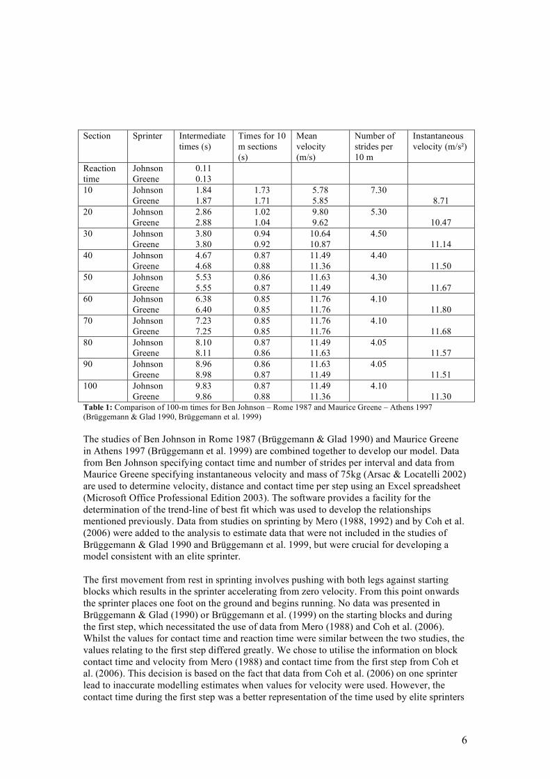
Table 1: Comparison of 100-m times for Ben Johnson – Rome 1987 and Maurice Greene – Athens 1997

(Brüggemann & Glad 1990, Brüggemann et al. 1999)

The studies of Ben Johnson in Rome 1987 (Brüggemann & Glad 1990) and Maurice Greene

in Athens 1997 (Brüggemann et al. 1999) are combined together to develop our model. Data

from Ben Johnson specifying contact time and number of strides per interval and data from

Maurice Greene specifying instantaneous velocity and mass of 75kg (Arsac & Locatelli 2002)

are used to determine velocity, distance and contact time per step using an Excel spreadsheet

(Microsoft Office Professional Edition 2003). The software provides a facility for the

determination of the trend-line of best fit which was used to develop the relationships

mentioned previously. Data from studies on sprinting by Mero (1988, 1992) and by Coh et al.

(2006) were added to the analysis to estimate data that were not included in the studies of

Brüggemann & Glad 1990 and Brüggemann et al. 1999, but were crucial for developing a

model consistent with an elite sprinter.

The first movement from rest in sprinting involves pushing with both legs against starting

blocks which results in the sprinter accelerating from zero velocity. From this point onwards

the sprinter places one foot on the ground and begins running. No data was presented in

Brüggemann & Glad (1990) or Brüggemann et al. (1999) on the starting blocks and during

the first step, which necessitated the use of data from Mero (1988) and Coh et al. (2006).

Whilst the values for contact time and reaction time were similar between the two studies, the

values relating to the first step differed greatly. We chose to utilise the information on block

contact time and velocity from Mero (1988) and contact time from the first step from Coh et

al. (2006). This decision is based on the fact that data from Coh et al. (2006) on one sprinter

lead to inaccurate modelling estimates when values for velocity were used. However, the

contact time during the first step was a better representation of the time used by elite sprinters

7

of world record standards. In addition, the data pertaining to an elite sprinter in Coh et al.

(2006) is used as a test case for the model in a subsequent analysis of a practical situation.

Results

Distance

(m)

Step number Calculated

instantaneous

velocity1 (m/s)

Calculated

time2 (s)

Distance

accumulated

per step3 (m)

Distance

travelled per

step (m)

Propulsion

force4 (kg)

0 0-block start 3.52 0.420 0.00 79.0

1 4.57 0.617 1.23 1.23 47.1

2 5.50 0.813 2.55 1.32 45.8

3 6.32 1.010 3.95 1.40 44.4

4 7.04 1.206 5.43 1.48 42.8

5 7.68 1.402 6.99 1.56 41

6 8.24 1.599 8.61 1.63 39.1

10 7 8.72 1.795 10.31 1.70 37.1

8 9.15 1.992 12.07 1.76 34.9

9 9.51 2.188 13.89 1.82 32.8

10 9.83 2.384 15.78 1.88 30.6

11 10.10 2.581 17.71 1.94 28.4

12 10.33 2.777 19.70 1.99 26.3

20 13 10.54 2.974 21.73 2.03 24.4

14 10.71 3.170 23.80 2.08 22.6

15 10.86 3.366 25.92 2.12 21

16 11.00 3.563 28.07 2.15 19.6

30 17 11.11 3.759 30.26 2.18 18.5

18 11.21 3.956 32.47 2.21 17.5

19 11.31 4.152 34.71 2.24 16.6

20 11.39 4.348 36.97 2.26 16

21 11.47 4.545 39.25 2.28 15.5

40 22 11.53 4.741 41.54 2.29 15

23 11.60 4.938 43.85 2.30 14.7

24 11.66 5.134 46.16 2.31 14.4

25 11.71 5.330 48.48 2.32 14.1

50 26 11.75 5.527 50.79 2.32 13.8

27 11.78 5.723 53.10 2.31 13

28 11.81 5.920 55.41 2.31 12

29 11.82 6.116 57.70 2.30 10.7

60 30 11.81 6.312 59.99 2.28 9.1

Table 2: Calculations of velocity, time, distance and propulsive force using formulae developed for our Newtonian

model. 1See Appendix 2,

2see Appendix 3,

3see Appendix 4,

4propulsion force=resultant impulse/contact time.

8

Velocity per step of Newtonian Model

y = -2E-05x4 + 0.0018x

3 - 0.0637x

2 +

1.1073x + 3.5238

R2 = 0.9998

0

2

4

6

8

10

12

14

0 4 8 12 16 20 24 28

Number of steps

Velo

city (

m/s

)

Contact time per step of Newtonian

Model

y = -0.0146x3 + 0.8411x

2 - 16.317x +

192.64

R2 = 0.9991

0

20

40

60

80

100

120

140

160

180

200

0 4 8 12 16 20 24 28

Number of steps

Conta

ct

tim

e (

ms)

Graph 1: Graph of velocity per stride showing the

formula that allows calculation of velocity for each

individual step (see Appendix 2)

Graph 2: Graph of contact time per stride showing

the formula that allows calculation of contact time

for each individual step (see Appendix 3)

Power per step of Newtonian Model

500

1000

1500

2000

2500

3000

3500

0 4 8 12 16 20 24 28

Number of steps

Pow

er

(Watt

s)

Force per step of Newtonian Model

0

10

20

30

40

50

60

70

80

90

0 4 8 12 16 20 24 28

Number of steps

Forc

e (

kg)

Graph 3: Graph of power per step. Graph 4: Graph of horizontal force per step.

The software provides a facility to determine the equation of the line of best fit to the data

which resulted in the following equations for this particular model:

Velocity per step = -0.00002x4 + 0.0018x

3 – 0.0637x

2 + 1.1073x

+ 3.5238 (R

2 = 0.9998)

Contact time per step = -0.0146x3 + 0.8411x

2 – 16.317x

+ 192.64 (R

2 = 0.9991)

Power per step = 0.00005x6 - 0.0052x

5 + 0.1642x

4 - 0.7955x

3 - 40.83x

2 + 498.17x + 1735.1

(R2 = 0.9999) from the first step onwards.

Force per step = -0.000005x5 + 0.0001x

4 + 0.0073x

3 + 0.1983x

2 - 0.6454x + 49.623

(R2 = 1) from the first step onwards

Discussion

For the calculated forces of the Newtonian model to be similar to real measurements the

estimation of drag force also needs to be real. Using the formula developed by Hill (1927),

the drag force due to air resistance was calculated to be 28N at a velocity of 10.10m/s which

is similar to that found by Pritchard & Pritchard (1994) of 27N at the same velocity. Davies

9

(1980) estimated that the force needed to overcome air resistance at 10m/s to be 7.8% of the

energy cost. The amount of force needed by the Newtonian model to overcome air resistance

is approximately 10% of total force produced at the same velocity.

Our model is designed to aid the coach or athlete in prescribing an appropriate force to train

against. Therefore the correct magnitude of the forces responsible for propelling the sprinter

throughout the various stages of the race is important. When maximal running at

9.59(±0.33)m/s between the 35 – 45m distance, Mero & Komi (1994) measured sprinters with

an average mass of 74.2(±7.6)kg to be producing a horizontal propulsive force of 338(±58)N.

This compares with the amount of force calculated for the Newtonian model at a similar

velocity of around 320N although our model reaches the same velocity much earlier in the

race during the 10th step and approximately 16m from the start of the race. Cavagna et al.

(1971) measured forces of 20 – 30kg at speeds of 8 – 10 m/s compared to our calculation of

the same forces between 10 – 11m/s. In fact our model produces greater forces when running

at the same speeds of athletes used in the study by Cavagna et al (1971). However, our model

represents a different class of athlete as our models reaches speeds of 8 – 10m/s within 3

seconds compared to 3 – 5 seconds for the athletes in the study by Cavagna et al. (1971).

The amount of force generated for our Newtonian model was calculated to be 775N in the

starting blocks. This is much lower than that measured by Mero (1988) who found a

horizontal maximal force production of 1216(±182)N. The result of our model is closer to the

average force produced by the sprinters in the same study of 655(±76)N. The amount of force

was calculated in our model to produce the velocity specified by the equation fitting velocity

to step number. If we substituted the values of contact time, mass and velocity when leaving

the blocks from the study by Mero (1988) we obtain a force of 750N which is still larger than

the average force of 655N. Nevertheless, the prospect of world-record breaking sprinters

producing higher block forces of less than 10kg is not an unreasonable assumption given the

high emphasis on strength training by the elite athlete who is nowadays a professional.

During the first step after the starting block, force is only applied with one leg as opposed to

two in the starting block. We calculated a force of 462N in the first step for our Newtonian

model which is much lower than that measured by Mero (1988) of 788(±96)N for maximal

force but within the range for the average force of 526(±75)N measured by Mero (1988). If a

lower magnitude of velocity was obtained out of the starting blocks the magnitude of force

produced in the first step would have been a lot closer. For example, a starting block velocity

of 3.38m/s for our model would have required the exact same force of 526N during the first

step in order to produce the same velocity after the first step.

The estimation of block velocity for the Newtonian model of 3.52m/s compares favourably

with that of 3.42(±0.32)m/s quoted in Mero (1988) from which our data were based. It can be

seen that the elite athlete represented by the Newtonian model is faster out of the starting

blocks. In slight contrast the velocity in the first step of the elite Newtonian model of 4.57m/s

is lower than 4.65(±0.28)m/s of Mero (1988), which is the data used in the velocity curve

fitting to develop our model. Similarly, Coh et al. (1998) measured a horizontal velocity of

4.47(±0.29)m/s after the first step, and a horizontal velocity of 5.38(±0.24)m/s after the

second step for athletes with average 100m times of 10.73s (±0.2). The velocity calculated for

the second step of our model is similar in value at 5.50m/s.

The production of force in sprinting is regarded as impulsive force due to the short time of

application. During the first step Mero (1988) measured an impulse of 90(±11)Ns compared

to our model of 79.5 Ns. Impulse of elite sprinters (100m time 10.75s, mass 69.5 kg) was

measured by Johnson & Buckley (2001) at approximately 14m from the starting blocks. They

observed a propulsive impulse of 26.3(±4.2)Ns and a braking impulse of 6.8(±2.4)Ns at a

10

mean velocity of 8.66(±0.37)m/s. We calculated a total impulse of around 32Ns for our model

at approximately the same distance from the starting blocks. However, our model reaches the

same velocity around 10m from the start and produces approximately 40Ns of impulse at that

distance. When adjusted for mass, our Newtonian model produces 38Ns of impulse with

69.5kg of mass (the same mass of Johnson & Buckley 2001) at the same velocity which is

still higher than that measured by Johnson & Buckley (2001) of propulsive impulse even

when it is combined with braking impulse at the same velocity.

The sprinters used by Mero & Komi (1994) produced a propulsive impulse of 20(±3)Ns at a

speed of 9.59m/s. However at the same velocity nearly 32Ns of impulse is produced by the

Newtonian model which is 60% greater. Furthermore, this occurred during the 9th step just

13m into the race for our model. Our model produces 20Ns of impulse at a distance of 21m

compared to the 35-40m of the athletes measured by Mero & Komi (1994). It seems that the

elite Newtonian model produces much higher impulses than lesser quality sprinters at the

same velocity. However, impulse is not a tool by which a coach or an athlete can readily use

for a training program except in more technological facilities that may also measure exercise

in terms of power.

With regard to power in sprinting, Mero & Komi (1994) calculated a propulsive power of

43.7(±8.0)W/kg at maximal velocities of 9.59m/s. Given that the average mass for the

sprinters is 74.2kg this would amount to 3242.5W or 3277.5W with the mass of the

Newtonian model at maximal velocity which is far greater than the power values calculated

for our model of approximately 1780 watts at the same distance of 35-40m from the start.

However, our model achieves the same velocity in the 9th step at 13m. In this region, our

model produces better results with approximately 3056 watts of power. This differs to that

measured by Mero & Komi (1994) by 7%. Our figure is similar to Cavagna et al. (1971) who

quoted between 2500-3000W at 9.5m/s. Similar values of power were reported at maximal

sprinting of 9.96m/s in the review by Mero et al. (1992) of 42W/kg in the propulsive phase.

This would have equated to 3150W if those subjects were of equal weight to our model. Our

model produces a power output of around 2900W at a similar velocity. Therefore, the power

of the Newtonian model compares reasonably with other studies at similar velocities.

The power generated by our model in the starting blocks is calculated to be 2732W generated

as the product of muscles from two legs. The amount of power generated as a result of the

propulsion of a single leg peaked around 3172W during the 7th step at a distance of 10m and

1.80s from the start. Horizontal power of 12.7W/kg was reported in the blocks by Mero et al.

(1992) for their athletes with 100m times of 10.80s, which would have equated to 952W

given the mass of our model. This large discrepancy compared to the Newtonian model of

2732W may be the reason for the difference between the velocity out of the starting blocks

between our Newtonian model (3.52m/s) and that reported in the review of 3.22m/s by Mero

et al. (1992). Even when the figures of block velocity and force production time from Mero et

al. (1992) are substituted into our Newtonian model, we still calculate a magnitude of power

more than twice that of Mero et al. (1992). This difference may be explained by that fact that

power in the Newtonian model is calculated from the final velocity instead of the average

velocity which is much lower in the starting blocks where velocity changes from zero.

The magnitudes for the Newtonian model of force, impulse, velocity, power and force

production times are similar to that measured by other researchers with the exception of the

power output at the start. Taking into account the distance over a 100m sprint, it can be seen

that the Newtonian model of an elite sprinter during a world record performance achieves

higher values for power, force and impulse at an earlier distance in the race than the

accomplished athletes measured by various researchers. Impulse is the product of force and

time whilst power is the product of force and velocity. This raises the question of what

mechanisms may be produced by the Newtonian model (representative of a world record

performance) compared to the athletes that aspire to achieve the same. Force, being the

11

common variable, could be the primary mechanism for running faster which agrees with

Weyand et al. (2000) although the magnitudes of horizontal forces are not high. Furthermore

force in this instance may not refer to traditional beliefs of force applied against the ground.

Force is related to the change in velocity over time (F = m(v-u)/t). The momentum of the legs

equals mass multiplied by velocity (mv). This could suggest that the velocity of the leg would

influence speed given the mass of the leg is constant. If so, this agrees with Alexander (1989)

who found very strong correlations between top speed and velocity of the leg during the

stance phase. In addition, the ability to change momentum within a small time frame (t) could

increase the magnitude of force. It must be recognised that the force that results in forward

motion of the sprinter might be a sum of different forces. These different forces could be

facilitated from many different factors; muscle force applied against the ground, velocity of

the leg prior to and/or during the ground contact phase, or the time in which force is applied

against the ground. Furthermore, any of these factors could be related to force generation that

is velocity dependent. The lesser sprinters may not have the ability to produce force at

specific velocities in specific biomechanical positions. Any deficiency in force production for

sprinting is most effectively addressed with velocity specific strength training (Behm & Sale

1993) and with similar movement specific strength training (Weiss 1991, Young 1992).

Newtonian model in practice

The Newtonian model provides a standard with which athletes can compare their own results.

For this purpose, we demonstrate the value of the Newtonian model herein and using data

published by Coh et al. (2006) describing the kinematics of Matic Osovnikar over a 20-m

sprint (Appendix 6) which he completed in 2.98 seconds (100m best 10.14s). The data were

examined using the same method of analysis and formulae for the Newtonian model.

Force produced by Matic Osovnikar

compared to Newtonian model

-20

0

20

40

60

80

100

120

140

160

0 1 2 3 4 5 6 7 8 9 10 11

Number of steps

Forc

e (

kg)

Matic Osovnikar

Newtonian model

Power output of Matic Osovnikar

compared to Newtonian model

-2000

0

2000

4000

6000

8000

10000

0 1 2 3 4 5 6 7 8 9 10 11

Number of steps

Pow

er

(W)

Matic Osovnikar

Newtonian model

Graph 5: Force generated by Matic Osovnikar

measured by Coh et al. (2006) compared to the

force calculated for the Newtonian model.

Graph 6: Power produced by Matic Osovnikar

compared to the power calculated for the

Newtonian model.

12

Change in velocity per step of Matic

Osovnikar compared to Newtonian model

-0.5

0.0

0.5

1.0

1.5

2.0

2.5

3.0

3.5

4.0

4.5

0 1 2 3 4 5 6 7 8 9 10 11

Number of steps

Change in v

elo

city (

m/s

)

Matic Osovnikar

Newtonian model

Graph 7: Change in velocity for each step taken

by Matic Osovnikar (Coh et al. 2006) compared

to that calculated for the Newtonian model.

Comparison of contact time per step of

Matic Osovnikar compared to

Newtonian model

90

100

110

120

130

140

150

160

170

180

190

1 2 3 4 5 6 7 8 9 10 11 12 13

Number of steps

Gro

und c

onta

ct

tim

e (

ms) Matic Osovnikar

Newtonian model

Graph 8: Ground contact time of Matic

Osovnikar (Coh et al. 2006) compared to that

calculated for the Newtonian model.

The data provided by Coh et al. (2006) on Matic Osovnikar shows a 51% loss of velocity

during the braking phase of the first step (Appendix 6). In order for Milan to produce the

propulsive velocity of 4.39m/s quoted, a total force of 122kg at a power output of 5248W

must be produced by Matic. These figures are much greater than those produced in the

Newtonian model for the first step. In contrast, Mero (1988) calculates an impulse in the

braking phase of -3Ns which reduced the velocity of the athletes in their study by 0.04m/s

from the velocity prior to landing of 3.46m/s equal to a loss of only 1%. Compared to athletes

in other studies Matic experiences a substantial loss of velocity during the first step.

From the information presented, a training plan needs to be put in place to prevent such a loss

of velocity within the first step. Alternatively, if the loss is unavoidable in real situational

sprinting, then training methods may need to focus on this area for maximal power

production. One possible solution would be to devise a unilateral jump squat in which case

the target in training should be to lift 122kg (including body weight) as fast as possible as

determined using the Newtonian formulae. In addition, the movement pattern should replicate

that of the actual position of the first step so as to obey the movement specificity of training

principle (Weiss 1991) similar to the single leg forward hack squat presented in a study by

Blazevich et al. (2003).

In comparison to the ground contact time as the race progresses for the Newtonian model, the

ground contact time for Matic Osovnikar fails to reduce at the same rate especially from the

10th step onwards. According to Murphy et al. (2003) in a study of non-elite athletes, ground

force contact times may be the difference between fast and slow runners over 10m. Kunz &

Kaufmann (1981) showed that world class sprinters had shorter ground force production

times than elite athletes that were not world class sprinters. This might suggest that between

elite sprinters the ability to continue to reduce ground contact times might be an important

factor. However it must be realized that the contact times represented in the Newtonian model

are presumptions and not actual average measurements except for the 7th and 12th steps. The

reality could be different as seen in the data presented for Matic whereby he executes steps 3,

4, 5 and 6 in around 130 milliseconds each. This behaviour is not duplicated in the other

sprints carried out by Matic that, when averaged, more closely represents the Newtonian

model (see Appendix 6).

It can be seen that the power produced by Matic diminishes during the 6th step as well as the

8th and 10th steps. This suggests that Matic is not productive with his left leg (given that his

13

right leg was the 1st step) during these particular steps. When analysing the force produced

during the 6th, 8th and 10th steps, the graph shows that Matic produces little propulsive force.

In fact, Matic experiences a loss of velocity during steps 8 and 10 which could be as a result

of the low propulsive force. Therefore, it seems relevant that this particular leg be

strengthened at the specific velocity of movement of around 7-9m/s attributable to those steps

(Behm & Sale 1993) using an exercise with a similar movement pattern (Weiss 1991). If the

coach or athlete needs to devise an exercise to strengthen that particular area of sprinting, the

resistance they choose to train with should be governed by the total horizontal force produced

at those velocities of between 30-40kg. Furthermore, unless velocity specific strength is

related to ground contact time, a training method that facilitates a reduction in the ground

contact time for Matic from the 10th step onwards could be of great value.

Conclusion

The values produced by our model for velocity are generally higher than those achieved in the

studies presented at similar stages in a 100-m sprint race. This is in line with our expectations

as our model is based on the world record performances of two elite athletes. Surprisingly,

our model does not clearly produce greater forces or comparative power output than the

athletes presented in the above studies, except for the values obtained in the starting blocks.

Whilst the magnitudes of the forces between our model and athletes presented in the above

studies are equivalent at similar velocities, the Newtonian model achieves the same velocity

as the athletes in comparative studies much earlier in the race. Perhaps the ability to achieve

greater velocities early in a sprint race is related to the ability to continue reducing the ground

force production time as seen when the Newtonian model is compared with the data of Matic

Osovnikar (Coh et al. 2006). More than likely there are many factors that influence sprinting

speed such as velocity and movement specific strength.

It must be noted that the values produced by our Newtonian model represent forces in the

horizontal direction only and are averaged over the period of contact. Additionally, we have

only specified the force, velocity and power that equate to the realised motion and do not take

into account the exact losses incurred within the musculoskeletal structure or losses incurred

due to friction. Nevertheless the estimation of such losses was taken into account using the

only data available. Generally, the magnitudes of the force, impulse and power were within

expectations compared to other studies.

The Newtonian model of an elite sprinter is developed from a set of formulas that allow

estimation of the fundamental quantities which can be related to the biomechanical position of

an athlete during the actual step taken. In particular, the formulas allow a calculation of force,

velocity, ground force contact time and distance travelled per step. These factors could be of

importance when prescribing or designing a plyometric exercise that focuses on speed or

distance, and also when teaching running technique. In addition, information gathered from

an athlete can be used to identify weaknesses, which can be addressed through strength

training, plyometric training, or specific changes to running technique.

The equations that produced the Newtonian model allow us to predict the force, time of force

production and power which results in realised motion for a world record sprint race. In this

respect, the Newtonian model can be used as a guideline for the force, velocity, and force

production times required of a world class sprinter. This gives the coach and the athlete a

guideline as to what resistance to train against, at what speed to train at and in what position

to use at training in order to provide specific velocity and movement specific training.

Accordingly, training with such specificity should transfer well into actual sprinting

performance.

14

References:

1. Alexander MJ. The relationship between muscle strength and sprint kinematics in elite

sprinters. Canadian Journal of Sport Science 14:3, 148-157.

2. Almasbakk, B and Hoff J. Coordination, the determinant of velocity specificity? Journal

of Applied Physiology 80(5): 2046-2052, 1996.

3. Arsac LM and Locatelli E. Modeling the energetics of 100-m running by using speed

curves of world champions. Journal of Applied Physiology 92: 1781-1788, 2002.

4. Babic V, Harasin D, Dizdar D. Relations of the variables of power and morphological

characteristics to the kinematic indicators of maximal speed running. Kinesiology

39(2007) 1:28-39.

5. Behm DG, and Sale DG. Velocity specificity of resistance training. Sports Medicine

15(6): 374-388, 1993.

6. Blazevich AJ, Gill ND, Bronks R, and Newton RU. Training-specific adaptation after

5-wk training in athletes. Medicine and Science in Sports and Exercise 35:2013-2022,

2003.

7. Blazevich AJ, and Jenkins DG. Effects of the movement speed of resistance training on

sprint and strength performance in concurrently training elite junior sprinters. Journal

of Sports Sciences 20, 981-990, 2002.

8. Brüggemann GP, and Glad B (Editors). Scientific Research Project at the games of the

XXXIV Olympiad- Seoul 1988: Final Report. International Athletic Federation.

Monaco, 1990.

9. Brüggemann GP, Koszewski D, and Müller H (Editors). Biomechanical Research

Project Athens 1997. Final Report. Oxford, UK: MMSU, 1999.

10. Cavagna GA, Komarek L, and Mazzoleni S. The mechanics of sprint running. Journal

of Physiology (1971), 217, pp. 709- 721.

11. Coh M, Bojan Jost, Branko Skof, Katja Tomazin, Ales Dolenec. Kinematic and kinetic

parameters of the sprint start and start acceleration model of top sprinters. Gymnica,

vol. 28, 1998.

12. Coh M, Tomazin K, Stuhec S. The biomechanical model of the sprint start and block

acceleration. Facta Universitatis - Series: Physical Education and Sport Vol. 4, No. 2,

2006, pp. 103 -114.

13. Davies CTM. Effects of wind assistance and resistance on the forward motion of a

runner. Journal of Applied Physiology: Respiration Environment Exercise Physiology

48(4): 702 – 709, 1980.

14. Delecluse C, Van Coppenolle H, Willems E, Van Leemputte M, Diels R, Goris M.

Influence of high-resistance and high-velocity training on sprint performance.

Medicine and Science in Sports and Exercise 27: 1203-1209, 1995.

15. Delecluse C. Influence of strength training on sprint running performance. Sports

Medicine 24(3): 147-156, 1997.

16. Gorostiaga EM., Izquierdo M, Ruesta M, Iribarren J, Gonzalez-Badillo JJ, Ibanez J.

Strength training effects on physical performance and serum hormones in young soccer

players. Eur J Appl Physiol (2004) 91: 698-707.

17. Harris GR, Stone MH, O’Bryant HS, Proulx CM, Johnson RL. Short-term performance

effects of high power, high force, or combined weight-training methods. Journal of

Strength and Conditioning Research, 2000, 14(1): 14-20.

18. Hill AV. The air resistance to a runner. Proceedings of the Royal Society, B, 102, 380-

385, 1928.

19. Hoffman JR, Cooper J, Wendell M, Kang J. Comparison of Olympic vs. traditional

power lifting training programs in football players. Journal of Strength and

Conditioning Research, 18(1): 129-135, 2004.

20. Hunter JP, Marshall RN, McNair PJ. Relationships between ground reaction force

impulse and kinematics of sprint-running acceleration. Journal of Applied

Biomechanics, 2005, 21, 31-43.

15

21. Johnson MD, and Buckley JG. Muscle power patterns in the mid-acceleration phase of

sprinting. Journal of Sports Sciences, 2001, 19, 263-272.

22. Kotzaminidis C, Chatzopoulos D, Michailidis C, Papaiakovou G, Patikas D. The effect

of a combined high-intensity strength and speed training program on the running and

jumping ability of soccer players. Journal of Strength and Conditioning Research,

19(2): 369-375, 2005.

23. Kristensen GO, Van Den Tillar R, Ettema G. Velocity specificity in early-phase sprint

training. Journal of Strength and Conditioning Research, 2006, 20(4), 833-837.

24. Kunz H, and Kaufmann DA. Biomechanical analysis of sprinting: decathletes versus

champions. British Journal of Sports Medicine, Vol. 15, No. 3, pp 177- 181, 1981.

25. Linthorne N.P. The effect of wind on 100-m sprint times. Journal of Applied

Biomechanics, 1994, 10, 110-131.

26. Lyttle AD, Wilson GJ, Ostrowski KJ. Enhancing performance: Maximal power versus

combined weights and plyometrics training. Journal of Strength and Conditioning

Research, 1996, 10(3), 173-179.

27. Majdell R, and Alexander MJL. The effect of overspeed training on kinematic variables

in sprinting. Journal of Human Movement Studies, 1991, 21, 19-39.

28. McBride JM, Triplett-McBride T, Davie A, Newton RU. The effect of heavy- vs. light-

loaded jump squats on the development of strength, power, and speed. Journal of

Strength and Conditioning Research, 2002, 16(1), 75-82.

29. Mero A. Force-time characteristics and running velocity of male sprinters during the

acceleration phase of sprinting. Research Quarterly for Exercise and Sport 1988, Vol.

59, No. 2, pp. 94-98.

30. Mero A, Komi PV, Gregor RJ. Biomechanics of sprint running. A review. Sports

Medicine 13 (6): 376-392, 1992.

31. Mero A, and Komi PV. EMG, force, and power analysis of sprint-specific strength

exercises. Journal of Applied Biomechanics, 1994, 10: 1-13.

32. Murphy AJ, Lockie RG, Coutts AJ. Kinematic determinants of early acceleration in

field sport athletes. Journal of Sports Science and Medicine (2003) 2, 144-150.

33. Di Prampero PE, Fusi S, Sepulcri L, Morin JB, Belli A, and Antonutto G. Sprint

running: a new energetic approach. Journal of Experimental Biology 208, 2809-2816,

2005.

34. Pritchard WG, and Pritchard JK. Mathematical models of running. American Scientist

82: 546-553, 1994.

35. Pugh L. The influence of wind resistance in running and walking and the mechanical

efficiency of work against horizontal or vertical forces. Journal of Physiology (1971),

213, pp. 255-276.

36. Rimmer E, and Sleivert G. Effects of a plyometrics intervention program on sprint

performance. Journal of Strength and Conditioning Research, 2000, 14 (3), 295-301.

37. Rutherford OM, and Jones DA. The role of learning and coordination in strength

training. European Journal of Applied Physiology, 55, 100-105, 1986.

38. Sale DG. Neural adaptations to strength training. In: Strength and Power in Sport (ed:

Paavo K. Komi), International Olympic Committee, Blackwell Science 1992.

39. Spinks CD, Murphy AJ, Spinks WL, Lockie RG. The effects of resisted sprint training

on acceleration performance and kinematics in soccer, rugby union, and Australian

football players. Journal of Strength and Conditioning Research, 2007, 21 (1), 77-85.

40. Summers, Richard L. Physiology and Biophysics of the 100-m sprint. News in

Physiological Sciences, Vol 12, June 1997.

41. Tricoli V, Lamas L, Carnevale R, Ugrinowitsch C. Short-term effects on lower-body

functional power development: weightlifting vs. vertical jump training programs.

Journal of Strength and Conditioning Research, 2005, 19(2), 433-437.

42. Ward-Smith A.J. New insights into the effect of wind assistance on sprinting

performance. Journal of Sports Sciences 1999, 17, 325-334.

16

43. Weiss, Lawrence W. The obtuse nature of muscular strength: the contribution of rest to

its development and expression. Journal of Applied Sports Science Research 1991,

Volume 5, Number 4, pp. 219-227.

44. Weyand PG, Sternlight DB, Bellezzi MJ, Wright S. Faster top running speeds are

achieved with greater ground forces not more rapid leg movements. Journal of Applied

Physiology 89: 1991-1999, 2000.

45. Wiemann K, and Tidow G. Relative activity of hip and knee extensors in sprinting-

implications for training. New Studies in Athletics, 10:1; 29-49, 1995.

46. Wilson G.J., Newton R.U., Murphy A.J., and Humphries B.J. The optimal training load

for the development of dynamic athletic performance. Medicine and Science in Sports

and Exercise 25:1279-86, 1993.

47. Wisloff U, C Castagna, J Helgerud, R Jones, J Hoff. Strong correlation of maximal

squat strength with sprint performance and vertical jump height in elite soccer players.

British Journal of Sports Medicine 2004; 38: 285-288.

48. Young W. Sprint bounding and the sprint bound index. Journal of Strength and

Conditioning Association 14: 18- 21, 1992.

49. Young W, McLean B, Ardagna J. Relationship between strength qualities and sprinting

performance. Journal of Sports Medicine and Physical Fitness 1995; 35: 13-19.

APPENDIX 1

Evaluation of time differential between Ben Johnson 1987 and Maurice Greene 1997

Data for Ben Johnson and Maurice Greene showing similar times for each 10m interval is

presented in Table A1. For the purposes of determining the velocity per step for our

Newtonian model, the assumption is made that the instantaneous velocity of Maurice Greene

is equal to that of Ben Johnson at each 10m distance.

Ben Johnson (Rome 1987) Maurice Greene (Athens 1997)

Total time

(s)

Time neglecting

reaction time (s)

Total time

(s)

Time neglecting

reaction time (s)

Differential

Reaction time 0.11 0.13

10m 1.84 1.73 1.84 1.71 1.2%

20m 2.86 2.75 2.88 2.75 0.0%

30m 3.80 3.69 3.80 3.67 0.5%

40m 4.67 4.56 4.68 4.55 0.2%

50m 5.53 5.42 5.55 5.42 0.0%

60m 6.38 6.27 6.40 6.27 0.0%

Ave. difference 0.3%

Table A1: Calculation of differential between the sprint times run by Ben Johnson in Rome 1987

(Brüggemann & Glad 1990) and Maurice Greene in Athens 1997 (Brüggemann et al. 1999)

17

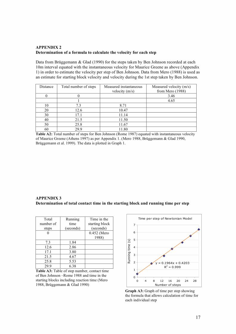
APPENDIX 2

Determination of a formula to calculate the velocity for each step

Data from Brüggemann & Glad (1990) for the steps taken by Ben Johnson recorded at each

10m interval equated with the instantaneous velocity for Maurice Greene as above (Appendix

1) in order to estimate the velocity per step of Ben Johnson. Data from Mero (1988) is used as

an estimate for starting block velocity and velocity during the 1st step taken by Ben Johnson.

Distance Total number of steps Measured instantaneous

velocity (m/s)

Measured velocity (m/s)

from Mero (1988)

0 0 3.46

1 4.65

10 7.3 8.71

20 12.6 10.47

30 17.1 11.14

40 21.5 11.50

50 25.8 11.67

60 29.9 11.80

Table A2: Total number of steps for Ben Johnson (Rome 1987) equated with instantaneous velocity

of Maurice Greene (Athens 1997) as per Appendix 1. (Mero 1988, Brüggemann & Glad 1990,

Brüggemann et al. 1999). The data is plotted in Graph 1.

APPENDIX 3

Determination of total contact time in the starting block and running time per step

Total

number of

steps

Running

time

(seconds)

Time in the

starting block

(seconds)

0 0.452 (Mero

1988)

7.3 1.84

12.6 2.86

17.1 3.80

21.5 4.67

25.8 5.53

29.9 6.38

Table A3: Table of step number, contact time

of Ben Johnson –Rome 1988 and time in the

starting blocks including reaction time (Mero

1988, Brüggemann & Glad 1990)

Time per step of Newtonian Model

y = 0.1964x + 0.4203

R2 = 0.999

0

1

2

3

4

5

6

7

0 4 8 12 16 20 24 28

Number of steps

Runnin

g t

ime (

s)

Graph A3: Graph of time per step showing

the formula that allows calculation of time for

each individual step

18

The relationship between running time and step suggests a time of 0.42 seconds is spent in the

starting blocks (i.e. step 0). Accounting for the reaction time of Ben Johnson of 0.11 seconds

(Brüggemann & Glad 1990), this equates to a time in the starting block of 0.31 seconds and is

taken as the contact time and reaction time in the starting block for the Newtonian model.

APPENDIX 4

Determination of a formula to calculate the distance per step

Total number of

steps

Distance (m)

7.3 10

12.6 20

17.1 30

21.5 40

25.8 50

29.9 60

Table A4: Table of distance and step number

for Ben Johnson -Rome 1988 (Brüggemann &

Glad 1990)

Distance per step of Newtonian

Model

y = -0.0006x3 + 0.0451x

2 +

1.1916x - 0.0051

R2 = 1

0

10

20

30

40

50

60

70

0 4 8 12 16 20 24 28

Number of steps

Dis

tance (

m)

Graph A4: Distance per step showing the

formula that allows calculation of distance for

each step

APPENDIX 5

Determination of an equation to calculate the contact time per step

Total number of

steps

Contact time (milliseconds) from

Bruggeman and Glad (1990)

Contact time (milliseconds) from

Coh et al. (2006)

0

1 177

7 115

12 91

17 85

21 87

25 80

29 80 (excluded from graph as relationship

is assumed to be constant after step 25)

Table A5: Table of step number and contact time of Ben Johnson -Rome 1988

(Brüggemann & Glad 1990, Coh et al. 2006)

In reference to graph 2, the polynomial trend line of best fit that will be used as the basis for

calculation of contact time for each stride of our model is:

y = -0.0146x3 + 0.8411x

2 - 16.317x + 192.64

19

However, this formula is not relevant to the contact time in the starting blocks as that is

produced with two legs as opposed to only one leg for all steps after the starting block.

Contact time in the starting blocks is estimated in Appendix 3.

APPENDIX 6

Information for Matic Osovnikar over 20-m (Coh et al. 2006) to determine the force, impulse,

and power using the same formulae applied in developing the Newtonian model.

Step Contact time for

best sprint (ms)

Average contact time

for 5 sprints (ms)

Flight

time (ms)

Total accumulated

distance (m)

Horizontal

velocity (m/s)

0 320 1.03 4.08

1 178 177 37 2.08 4.88*

2 179 159 80 3.44 5.25

3 129 136 92 4.84 6.33

4 130 131 92 6.39 6.98

5 129 120 86 8.03 7.63

6 130 123 98 9.80 7.76

7 117 120 111 11.71 8.42

8 111 112 117 13.61 8.29

9 98 103 111 15.57 9.38

10 105 110 123 17.65 9.12

11 104 111 19.79 9.95

12 105

Table A6: Information on Matic Osovnikar over a 20-m sprint adapted from Coh et al. (2006) during

the best run of 2.98 seconds. *Differs from 4.39 m/s quoted in text.

Block velocity (m/s) Step 1 (m/s) Step 2 (m/s)

Braking phase 2.00 5.98

Acceleration phase 4.11 4.41 6.00

Table A7: Horizontal velocity during the first steps of Matic Osovnikar over a 20-m sprint modified

from Coh et al. (2006) averaged over 5 sprints.