Newton’s Method on a System of Nonlinear

Equations

Nicolle Eagan, University at Bu↵aloGeorge Hauser, Brown University

Research Advisor: Dr. Timothy Flaherty, Carnegie Mellon University

Abstract

Newton’s method is an algorithm for finding the roots of di↵erentiable

functions, that uses iterated local linearization of a function to approxi-

mate its roots. Newton’s method also extends to systems of n di↵eren-

tiable functions in n variables. In this paper, we examine the dynamics of

Newton’s method on system of two bivariate polynomials. We explore the

generalization of Newton’s method to systems of two bivariate polynomi-

als, as well as techniques of computer visualization for the corresponding

dynamics. In particular, we investigate whether the attracting cycles that

arise in the dynamics of Newton’s Method on certain cubic polynomials

of one complex variable also arise in the case of bivariate quadratics.

1 Introduction

Complex dynamics is defined as the study of dynamical systems in the contextof iterated function systems in the complex plane. It is a broad field that canbe examined through many di↵erent perspectives, including Newton’s method.Newton’s method, applied to a polynomial equation, allows us to approximateits roots through iteration. Newton’s method is e↵ective for finding roots ofpolynomials because the roots happen to be fixed points of Newton’s method,so when a root is passed through Newton’s method, it will still return the exactsame value. We can see that the points found through iteration of Newton’smethod correspond to distinct components of the Fatou set. From this, we candetermine a function’s basins of attraction- a set of starting points in whicheach point in the set iterates to a particular root. Since this can be easilydone for one polynomial, we will consider a system of two nonlinear equations.We will see that by iterating Newton’s method on the inverse of the Jacobianmatrix for the system, we can calculate the distance for each root and createan image which displays the basins of attraction for the system. We will seethat the quadratic systems behave quite like the one variable case, while othersystems show interesting results. We will also see that the quadratic systemsbehave quite like the one-variable case, in that no attracting cycles will be found;

1

however in other systems, attracting cycles may exist due to the fact that thereexists cases where the second derivative maps to noninvertible matrices.

2 Complex Dynamics and Newton’s Method

2.1 Newton’s Method

As we have said, Newton’s method is an iterative algorithm for finding the rootsof a di↵erentiable function. But before we define Newton’s method precisely,let us make a few normalizing assumptions. In this paper, we will considerNewton’s method applied specifically to polynomials either real or complex.The advantage to working with polynomials specifically is that they are wellbehaved, in that they are infinitely di↵erentiable and have at most finitely manyroots and critical points. The advantage to working over C is that every nonconstant polynomial over C has at least one complex root, by the fundamentaltheorem of algebra.

So let us now define Newton’s method. Let f : C ! C be polynomial witha root ↵, so that f(↵) = 0. Let z0 be a point chosen roughly to approximate↵. Given that f is di↵erentiable at z0 we may construct an even better betterapproximation z1 of ↵ as follows. First we locally linearization of f at z0. Thisgives us an a�ne function L

z0 : C ! C whose graph is tangent to f at z0, givenby

L

z0(z) = f

0(z0)(z � z0) + f(z0)

Assuming that f

0(z0) 6= 0, we may solve the linear equation L

z0(z) = 0 anddenote the solution z1:

z1 = z0 �f(z0)

f

0(z0)

(We note that this assumption is valid for all but finitely many z0 since f has atmost finitely many critical points). Iterating this process, we obtain a sequenceof points (z

n

)n

that converges, as we will see, to ↵, provided that z0 is chosensu�ciently close to ↵ to begin with.

Here is a minor, though theoretically preferable, abstraction of the aboveoutlined procedure:

Given a polynomial f , define the Newton’s function of f , denoted N = N

f

,given by

N(z) = N

f

(z) = z � f(z)

f

0(z)

Here we generally consider the domain and range of N to be the Riemann sphere(i.e. C [1) so that N is defined even at singularities of f .

Now, from this perspective, Newton’s method can be seen as the iterationof Newton’s function on a starting point z0 that is su�ciently close to ↵.

2

2.2 Attracting Fixed Points and Basins of Attraction

We make the following useful observation:

Observation The roots of a polynomial f are precisely the fixed points of Nf

.

Proof. Suppose ↵ is a fixed point of N . Then N(↵) = ↵ � f(↵)f

0(↵) = ↵ only if

f(↵) = 0.In the other direction, suppose ↵ is a root of f of multiplicity m. Then

f(z) = (z � ↵)mq(z) where q is a polynomial such that q(↵) 6= 0. We compute

N(z) = z � (z � ↵)mq(z)

m(z � ↵)m�1q(z) + (z � ↵)mq

0(z)

= z � (z � ↵)q(z)

mq(z) + (z � ↵)q0(z)

Now, since q(↵) 6= 0, it follows that N(↵) = ↵.

In addition, roots of f are actually what are known as attracting fixed pointsof N .

Definition A fixed point ↵ of N is said to be attracting if |N 0(↵)| < 1. In thespecial case that N 0(↵) = 0, ↵ is said to be super-attracting.

To see that roots of f are attracting fixed points of N , we compute that

N

0(z) =f(z)f 00(z)

[f 0(z)]2

Once again using the factorization f(z) = (z�↵)mq(z), one checks that N 0(↵) =1 � 1/m, where m is the multiplicity of ↵ as a root of f . Therefore roots of fare generally attracting fixed points of N , and moreover single roots are super-attracting fixed points of N .

The technical use of the word “attracting” here is motivated by the local dynam-ics of N near its attracting fixed points. Imprecisely put, N “pulls” points closeto an attracting fixed point ↵ closer to ↵. Here is the more rigorous version.

Proposition 2.1. Let ↵ be an attracting fixed point of N . Then the sequence(N,N � N,N

�3, . . . ) of iterates of N converges uniformly to ↵ on some neigh-

borhood of ↵.

Proof. The proof of this proposition follows from considering the Taylor expan-sion of N about ↵.

This proposition justifies the previously made claim that Newton’s methodapplied to a starting point su�ciently close to a root of f will necessarily con-verge to that root.

3

Moreover, this proposition also implies that any starting point that eventu-ally iterates into such a neighborhood of a root will converge to that root. Thismotivates the following definition

The basin of attraction of an attracting fixed point of N is the set of pointsthat converge to that fixed point under iteration of N .

We note that the basin of attraction itself is an open set.

Basins of attractions of attracting fixed points of N can be visualized withcomputers in the following way. Create a grid of points representing a points inthe complex plane. Iterate Newton’s method on each of these points. Then colorpoints that converge to di↵erent attracting fixed points of N di↵erent colors.

The following figure illustrates this by visualizing the basins of attraction ofa cubic polynomial whose roots form the vertices of an equilateral triangle inthe complex plane.

4

−1 −0.5 0 0.5 1 1.5 2 2.5−2

−1.5

−1

−0.5

0

0.5

1

1.5

2

Figure 1: Newton basins for f(z) = (z

2+ 1)(z �

p3) in C.

In this image, red represents the basin for the root i, green represents the basinfor the root �i, and blue represents the basin for the root

p3. We see three

main regions emerge, separated by “bead-shaped” lines. Each main region is adi↵erent color, meaning each root has a main region of iteration.

2.3 Julia and Fatou Sets

In the above image, we note that almost every point iterates to one of the threeroots. However, we notice points that do not iterate to any root are locatedon the boundary of the basins. This is known as the Julia set [3]. The Juliaset is the set on which the dynamics of N are chaotic. One was to see thisis to consider a point on the boundary between two basins of attraction. Weobserve that any neighborhood of that point contains points in multiple basinsof attraction. Thus, under iteration of N , this neighborhood gets “torn apart”because di↵erent parts of the neighborhood get pulled to di↵erent roots.

The Fatou set is the complement of the Julia set; it is the set on which thedynamics of N are “well-behaved”. More rigorously, it is a set with regularbehavior in which the sequence of iterates is a normal family in some neighbor-hood of a set of points in C. Thus, the sequence of iterates is equicontinuousin the Fatou set. The Fatou set also contains basins of attraction of attractingfixed points. We now arrive at the following question: is the Fatou set entirelybasins of attraction for attracting fixed points? Let us consider the basins ofanother cubic polynomial.

5

Figure 2: Newton basins for f(z) = (z

2+ 1)(z � 4.5) in C.

We note that red represents the basin for the root i, green represents thebasin for the root �i, and blue represents the basin for the root 4.5. We nowobserve the roughly circular black regions in the image. These black regions,which have positive area, do not iterate to any of the roots. If we pick thestarting point z0 = 1.4997, one calculates that x1 = N(x0) ⇡ �0.1957 andN(x1) ⇡ 1.4997 = x0. Thus, what is known as a two-cycle emerges.

Moreover, it is in fact the case the the black regions, in some sense, representthe basin of attraction for this two cycle, in the sense that points in these regionsconverge under iteration of N to the two cycle.

We make this precise as follows. Denote the two-cycle by {x1, x2}, so thatN(x1) = x2 and N(x2) = x1. Also denote N

�2 = N � N . Observe thatN

�2(xi

) = x

i

for both i = 1, 2. From this perspective, both elements of thetwo-cycle are fixed points of N�2. Let us check the derivative of N�2 at both x1

and x2. Using the chain rule, we see that

(N �N)0(x1) = N

0(N(x1))N0(x1) = N

0(x2)N0(x1)

Likewise,(N �N)0(x2) = N

0(x1)N0(x2)

Plugging in our values, we see:

N

0(x1) = 5.998025658, N

0(x2) = 0.0004937078289

6

N

0(x1)N0(x2) = 0.002961272225 < 1

Therefore, both x1 and x2 are attracting fixed points of N�2, and this isprecisely what we mean when we refer the two-cycle {x1, x2} as an attractingtwo-cycle of N .

Therefore, these are attracting fixed pints of N�2. We now note the followingtheorem about cycles:

Theorem 1. An attracting cycle of N attracts at least one critical point of N[4].

This follows from the fact that all basins of attraction contain at least onecritical point of the function. Thus, N 0(x) = 0 implies f(x) = 0 or f

00(x) = 0.So, if there is an attracting cycle that is not trivial (i.e. not a fixed point or aone-cycle), then it attracts an inflection point of f , or a root of f 00. However,if f has degree d, then f

00 has degree d � 2, hence there can be at most d � 2non-trivial attracting cycles.

3 Newton’s Method in Several Variables

Newton’s method can be generalized for finding zeros of systems of n functions inn variables. For our purposes, we consider systems of two bivariate polynomials.

The idea of Newton’s method in two variables is the same as in one variable.Just like the one variable case, we choose a starting point, locally linearize, solvethe system of linear equations, and repeat.

First, we formalize the notion of a system of equations as a single, vector-valued function

f = (f1, f

2) : R2 ! R2

Like the one variable case, we find the local linearization of f at a vector v0 =(x0, y0) 2 R2 is given by L

v0(v) = J

v0(v � v0) + f(v0). Here, Jv0 represents

the Jacobian matrix of f at v0, which is a multivariable generalization of thederivative:

J(x0,y0) =

✓f

1x

f

1y

f

2x

f

2y

◆ �����(x0,y0)

where f

1x

is the partial derivative of f1 with respect to x, and likewise for theother entries of the matrix. Assuming J

v0 is invertible, we can solve the linearsystem L

v0(v) = 0 for v. We calculate:

v1 = v0 � J

�1v0

f(v0)

As in the one variable case, this motivates definition of the Newton function off : N = N

f

: R2 ! R2, given by:

N(v) = v � J

�1v

f(v)

7

Thus, Newton’s method in two variables can be seen as iteration of N . Essen-tially, start at a vector v0, then recursively define v

n+1 = N(vn

) until withinthe desired accuracy of a root.

4 Results

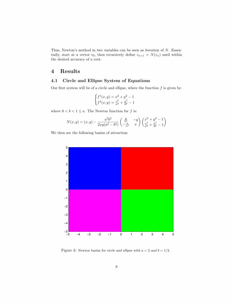
4.1 Circle and Ellipse System of Equations

Our first system will be of a circle and ellipse, where the function f is given by:

(f

1(x, y) = x

2 + y

2 � 1

f

2(x, y) = x

2

a

2 + y

2

b

2 � 1

where 0 < b < 1 a. The Newton function for f is:

N(x, y) = (x, y)� a

2b

2

2xy(a2 � b

2)

✓y

b

2 �y

� x

a

2 x

◆✓x

2 + y

2 � 1x

2

a

2 + y

2

b

2 � 1

◆

We then see the following basins of attraction:

−5 −4 −3 −2 −1 0 1 2 3 4 5−5

−4

−3

−2

−1

0

1

2

3

4

5

Figure 3: Newton basins for circle and ellipse with a = 2 and b = 1/2.

8

We notice that the dynamics of the system are quite simple. There are fourroots; one root per quadrant. This makes sense with what the image is showing,because each quadrant is a di↵erent color, meaning each quadrant iterates to adi↵erent root.

4.2 Quadratic System of Equations

We know consider another system of quadratic equations, namely

(f

1(x, y) = x

2 � y

f

2(x, y) = y

2 � x

Newton’s function is

N(x, y) = (x, y)� 1

4xy � 1

✓2y 11 2x

◆✓x

2 � y

y

2 � x

◆

9

The following is the image produced:

Figure 4: Newton basins for {x2 � y, y

2 � x}

Seeing theses basins of attraction, let’s examine the roots of the system, which

are (0, 0), (1, 1), (� 12 +

p32 i,� 1

2 �p32 i), and(� 1

2 �p32 i,� 1

2 +p32 i). We observe

two of these roots have complex coordinates. Thus, we can consider our functionf as a function f : C2 ! C2 (C2 represents the set of two-tuples of complexnumbers).

However, basins of attraction in C2 are hard to visualize, since C2 is four-dimensional over R. So, to visualize basins of attraction in C2, we take two-dimensional slices of C2. Three linearly independent vectors, v, w, and u in C2,define a 2-D slice:

{av + bw + u : a, b 2 R}

The previously shown basins of attraction in two variables were both theR2 slice, generated by the vectors v = (1, 0), w = (0, 1), and u = (0, 0). Wenote that dynamics are generally more interesting on slices that include three ormore roots. Using this technique, we can know visualize the following images:

We see very interesting dynamics appear in all of these images. We see“feather-like swirls” appearing in close-ups just o↵ of the origin. These basins

10

Figure 5: Newton basins for {x2 � y, y

2 � x}.Slice generated by v = (1, 1), w = (⇣3, ⇣

23 ), and

u = (0, 0)

Figure 6: Newton basins for {x2 � y, y

2 � x}.Slice generated by v = (1, 1), w = (⇣3, ⇣

23 ), and

u = (0, 0)

Figure 7: Newton basins for {x2�y, y

2�x}. Slice generated by v = (1, 1), w = (⇣3, ⇣23 ),

and u = (0, 0)

of attraction are quite intricate and are a very interesting result.

11

Figure 8: Newton basins for {x2 � y, y

2 � x}.Slice generated by v = (1, 1), w = (⇣3, ⇣

23 ), and

u = (0, 0)

Figure 9: Newton basins for {x2 � y, y

2 � x}.Slice generated by v = (1, 1), w = (⇣3, ⇣

23 ), and

u = (0, 0)

4.3 Another Quadratic System of Equations

Our results thus far have not exhibited any attracting cycles. Thus, we now con-sider a system of two polynomials in two variables that ought to have attractingcycles: (

(x2 + 1)(y � c)

(y2 + 1)(x� c)

for c = 9/2. The roots for this system are (c, c), (i,�i), (i, i), (�i, i), (�i,�i).We also calculate that the Newton function is as follows:

N(x, y) =

�x y

�� 1

det

✓x

2+ 1 �2y(x� c)

�2x(y � c) y

2+ 1

◆✓(y

2+ 1)(x� c)

(x

2+ 1)(y � c)

◆

where det = �3x

2y

2+ x

2+ y

2+ 1 + 4xy(xc + yc � c

2) The following basins of

attraction appear:

Figure 10: Basins of attraction for {(x2 +1)(y�4.5), (y2 + 1)(x � c)}, y=x slice.

Figure 11: Basins of attraction for {(x2 +1)(y�4.5), (y2 + 1)(x � c)}, y=x slice translated.

12

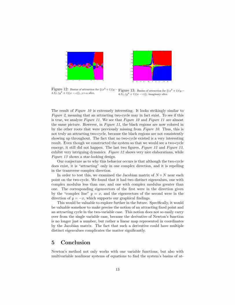
Figure 12: Basins of attraction for {(x2 +1)(y�4.5), (y2 + 1)(x � c)}, y=-x slice.

Figure 13: Basins of attraction for {(x2 +1)(y�4.5), (y2 + 1)(x � c)}, imaginary slice.

The result of Figure 10 is extremely interesting. It looks strikingly similar toFigure 2, meaning that an attracting two-cycle may in fact exist. To see if thisis true, we analyze Figure 11. We see that Figure 10 and Figure 11 are almostthe same picture. However, in Figure 11, the black regions are now colored inby the other roots that were previously missing from Figure 10. Thus, this isnot truly an attracting two-cycle, because the black regions are not consistentlyshowing up throughout. The fact that no two-cycle existed is a very interestingresult. Even though we constructed the system so that we would see a two-cycleemerge, it still did not happen. The last two figures, Figure 12 and Figure 13,exhibit very intriguing dynamics. Figure 12 shows very nice elaborations, whileFigure 13 shows a star-looking design.

Our conjecture as to why this behavior occurs is that although the two-cycledoes exist, it is “attracting” only in one complex direction, and it is repellingin the transverse complex direction.

In order to test this, we examined the Jacobian matrix of N �N near eachpoint on the two-cycle. We found that it had two distinct eigenvalues, one withcomplex modulus less than one, and one with complex modulus greater thanone. The corresponding eigenvectors of the first were in the direction givenby the “complex line” y = x, and the eigenvectors of the second were in thedirection of y = �x, which supports our graphical findings.

This would be valuable to explore further in the future. Specifically, it wouldbe valuable somehow to make precise the notion of an attracting fixed point andan attracting cycle in the two-variable case. This notion does not so easily carryover from the single variable case, because the derivative of Newton’s functionis no longer just a number, but rather a linear map represented in coordinatesby the Jacobian matrix. The fact that such a derivative could have multipledistinct eigenvalues complicates the matter significantly.

5 Conclusion

Newton’s method not only works with one variable functions, but also withmultivariable nonlinear systems of equations to find the system’s basins of at-

13

traction. Through our investigations, we saw Newton’s method reveals inter-esting dynamical behavior in several variables, but we were unable to find anytrue attracting cycles. There were several behaviors we observed that we wouldlove to research further in the future, such as actually finding a true attractingcycle, if one exists. It would also be interesting to explore the dynamics of morecomplicated nonlinear systems to see if any more interesting appear, and to alsosee if any characteristics of previously explored systems hold.

References

[1] Blanchard, P., ”The Dynamics of Newton’s Method” Proceedings of Sym-posia in Applied Mathematics, Vol. 49, pp. 139-155, 1994.

[2] Hubbard, J., Schleicher, D., Sutherland, S., How to Really Find Roots ofPolynomials by Newton’s Method, December 17, 1998.

[3] Alexander, D., Devaney, R., A Century of Complex Dynamics, April 1, 2014.

[4] Milnor, J., Dynamics in One Complex Variable, Third Edition. PrincetonUniversity Press, Princeton, New Jersey, 2006.

14