NEWTON SKETCH: A NEAR LINEAR-TIME OPTIMIZATION ALGORITHMWITH LINEAR-QUADRATIC CONVERGENCE

MERT PILANCI† AND MARTIN J. WAINWRIGHT†‡

Abstract. We propose a randomized second-order method for optimization known as the Newton Sketch: it isbased on performing an approximate Newton step using a randomly projected Hessian. For self-concordant functions,we prove that the algorithm has super-linear convergence with exponentially high probability, with convergence andcomplexity guarantees that are independent of condition numbers and related problem-dependent quantities. Given asuitable initialization, similar guarantees also hold for strongly convex and smooth objectives without self-concordance.When implemented using randomized projections based on a sub-sampled Hadamard basis, the algorithm typicallyhas substantially lower complexity than Newton’s method. We also describe extensions of our methods to programsinvolving convex constraints that are equipped with self-concordant barriers. We discuss and illustrate applications tolinear programs, quadratic programs with convex constraints, logistic regression and other generalized linear models, aswell as semidefinite programs.

Key words. Convex optimization, large-scale problems, Newton’s Method, random projection, randomized algo-rithms, random matrices, self-concordant functions, interior point method

AMS subject classifications. 49M15, 90C06, 90C25, 90C51, 62J12

1. Introduction. Relative to first-order methods, second-order methods for convex optimizationenjoy superior convergence in both theory and practice. For instance, Newton’s method convergesat a quadratic rate for strongly convex and smooth problems. Even for functions that are weaklyconvex—that is, convex but not strongly convex—modifications of Newton’s method have super-linearconvergence (for instance, see the paper [39] for an analysis of the Levenberg-Marquardt Method).This rate is faster than the 1/T 2 convergence rate that can be achieved by a first-order method likeaccelerated gradient descent, with the latter rate known to be unimprovable (in general) for first-order methods [27]. Yet another issue in first-order methods is the tuning of step size, whose optimalchoice depends on the strong convexity parameter and/or smoothness of the underlying problem. Forexample, consider the problem of optimizing a function of the form x 7→ g(Ax), where A ∈ R

n×d

is a “data matrix”, and g : Rn → R is a twice-differentiable function. Here the performance of

first-order methods will depend on both the convexity/smoothness of g, as well as the conditioningof the data matrix. In contrast, whenever the function g is self-concordant, then Newton’s methodwith suitably damped steps has a global complexity guarantee that is provably independent of suchproblem-dependent parameters.

On the other hand, each step of Newton’s method requires solving a linear system defined by theHessian matrix. For instance, in application to the problem family just described involving an n × ddata matrix, each of these steps has complexity scaling as O(nd2) assuming n ≥ d without loss ofgenerality. For this reason, both forming the Hessian and solving the corresponding linear systempose a tremendous numerical challenge for large values of (n, d)— for instance, values of thousandsto millions, as is common in big data applications. In order to address this issue, a wide variety ofdifferent approximations to Newton’s method have been proposed and studied. The general class ofquasi-Newton methods are based on estimating the inverse Hessian using successive evaluations ofthe gradient vectors. Examples of such quasi-Newton methods include DFP and BFGS schemes aswell their limited memory versions; see the book by Wright and Nocedal [38] and references thereinfor further details. A disadvantage of such first-order Hessian approximations is that the associatedconvergence guarantees are typically weaker than those of Newton’s method and require strongerassumptions.

In this paper, we propose and analyze a randomized approximation of Newton’s method, knownas the Newton Sketch. Instead of explicitly computing the Hessian, the Newton Sketch method ap-proximates it via a random projection of dimension m. When these projections are carried out usingthe fast Johnson-Lindenstrauss (JL) transform, say based on Hadamard matrices, each iteration hascomplexity O(nd log(m)+dm2). Our results show that it is always sufficient to choose m proportionalto min{d, n}, and moreover, that the sketch dimension m can be much smaller for certain types of

†Department of Electrical Engineering and Computer Science, University of California, Berkeley.‡Department of Statistics, University of California, Berkeley.

1

constrained problems. Thus, in the regime n > d and with m ≍ d, the complexity per iteration canbe substantially lower than the O(nd2) complexity of each Newton step. For instance, for an objec-tive function of the form f(x) = g(Ax) in the regime n ≥ d2, the complexity of Newton Sketch periteration is O(nd log d), which (modulo the logarithm) is linear in the input data size nd. Thus, thecomputational complexity per iteration is comparable to first-order methods that have access only tothe gradient AT g′(Ax). In contrast to first-order methods, we show that for self-concordant functions,the total complexity of obtaining a δ-approximate solution is O

(nd(log d) log(1/δ)

), and without any

dependence on constants such as strong convexity or smoothness parameters. Moreover, for problemswith d > n, we provide a dual strategy that effectively has the same guarantees with roles of d and nexchanged.

We also consider other random projection matrices and sub-sampling strategies, including partialforms of random projection that exploit known structure in the Hessian. For self-concordant functions,we provide an affine invariant analysis proving that the convergence is linear-quadratic and the guar-antees are independent of various problem parameters, such as condition numbers of matrices involvedin the objective function. Finally, we describe an interior point method to deal with arbitrary convexconstraints, which combines the Newton sketch with the barrier method. We provide an upper boundon the total number of iterations required to obtain a solution with a pre-specified target accuracy.

The remainder of this paper is organized as follows. We begin in Section 2 with some backgroundon the classical form of Newton’s method, past work on approximate forms of Newton’s method,random matrices for sketching, and Gaussian widths as a measure of the size of a set. In Section 3,we formally introduce the Newton Sketch, including both fully and partially sketched versions forunconstrained and constrained problems. We provide some illustrative examples in Section 3.3 beforeturning to local convergence theory in Section 3.4. Section 4 is devoted to global convergence resultsfor self-concordant functions, in both the constrained and unconstrained settings. In Section 5, weconsider a number of applications and provide additional numerical results. The bulk of our proofsare in given in Section 6, with some more technical aspects deferred to the appendices.

2. Background. We begin with some background material on the standard form of Newton’smethod, past work on approximate or stochastic forms of Newton’s method, the basics of randomsketching, and the notion of Gaussian width as a complexity measure.

2.1. Classical version of Newton’s method. In this section, we briefly review the convergenceproperties and complexity of the classical form of Newton’s method; see the sources [38, 6, 27] forfurther background. Let f : Rd → R be a closed, convex and twice-differentiable function that isbounded below. Given a convex and closed set C, we assume that the constrained minimizer

x∗ : = argminx∈C

f(x)(2.1)

exists and is uniquely defined. We define the minimum and maximum eigenvalues γ = λmin(∇2f(x∗))and β = λmax(∇2f(x∗)) of the Hessian evaluated at the minimum.

We assume moreover that the Hessian map x 7→ ∇2f(x) is Lipschitz continuous with modulus L,meaning that

|||∇2f(x+∆)−∇2f(x)|||op ≤ L ‖∆‖2.(2.2)

Under these conditions and given an initial point x0 ∈ C such that ‖x0 − x∗‖2 ≤ γ2L , the Newton

updates are guaranteed to converge quadratically—viz.

‖xt+1 − x∗‖2 ≤ 2L

γ‖xt − x∗‖22,

This result is classical: for instance, see Boyd and Vandenberghe [6] for a proof. Newton’s methodcan be slightly modified to be globally convergent by choosing the step sizes via a simple backtrackingline-search procedure.

The following result characterizes the complexity of Newton’s method when applied to self-concordant functions and is central in the development of interior point methods (for instance, seethe books [28, 6]). We defer the definitions of self-concordance and the line-search procedure to the

2

following sections. The number of iterations needed to obtain a δ-approximate minimizer of a strictlyconvex self-concordant function f is at most

20− 8a

ab(1− 2a)

(f(x0)− f(x∗)

)+ log2 log2(1/δ) ,

where a, b are constants in the line-search procedure.∗

2.2. Approximate Newton methods. Given the complexity of the exact Newton updates,various forms of approximate and stochastic variants of Newton’s method have been proposed, which wediscuss here. In general, inexact solutions of the Newton updates can be used to guarantee convergencewhile reducing overall computational complexity [11, 12]. In the unconstrained setting, the Newtonupdate corresponds to solving a linear system of equations, and one approximate approach is truncatedNewton’s method: it involves applying the conjugate gradient (CG) method for a specified number ofiterations, and then using the solution as an approximate Newton step [12]. In applying this method,the Hessian need not be formed since the CG updates only need access to matrix-vector productswith the Hessian. These matrix vector products can also be approximated using finite differences ofgradients (e.g., see [23]). While these strategies are popular, theoretical analysis of inexact Newtonmethods typically need strong assumptions on the eigenvalues of the Hessian [11]. Since the numberof steps of CG for reaching a certain residual error necessarily depends on the condition number, theoverall complexity of truncated Newton’s Method is problem-dependent; the condition numbers canbe arbitrarily large, and in general are unknown a priori. Ill-conditioned Hessian system are commonin applications of Newton’s method within interior point methods. Consequently, software toolboxestypically perform approximate Newton steps using CG updates in earlier iterations, but then shift toexact Newton steps via Cholesky or QR decompositions in later iterations.

A more recent line of work, inspired by the success of stochastic first-order algorithms for large scalemachine learning applications, has focused on stochastic forms of second-order optimization algorithms(e.g., [33, 5, 7, 8]). Schraudolph et al. [33] use online limited memory BFGS-like updates to maintainan inverse Hessian approximation. Byrd et al. [8, 7] propose stochastic second-order methods that usebatch sub-sampling in order to obtain curvature information in a computationally inexpensive manner.These methods are numerically effective in problems in which objective consists of a sum of a largenumber of individual terms; however, their theoretical analysis again involves strong assumptions onthe eigenvalues of the Hessian. Moreover, such second-order methods do not retain the affine invarianceof the original Newton’s method, which guarantees iterates are independent of the coordinate systemand conditioning. When simple stochastic schemes like sub-sampling are used to approximate theHessian, affine invariance is lost, since subsampling is coordinate and conditioning dependent. Incontrast, the stochastic form of Newton’s method analyzed in this paper is constructed so as to retainthis affine invariance property, and thus not depend on the problem conditioning.

2.3. Different types of randomized sketches. Our Newton sketch algorithm is based onperforming a form of dimensionality reduction using random matrices, known as sketching matrices.Various types of randomized sketches are possible, and we describe a few of them here. Given a sketch-ing matrix S ∈ R

m×n, we use {si}mi=1 to denote the collection of its n-dimensional rows. We restrictour attention to sketch matrices that are zero-mean, and that are normalized so that E[STS/m] = In.

Sub-Gaussian sketches. The most classical sketch is based on a random matrix S ∈ Rm×n with

i.i.d. standard Gaussian entries, or somewhat more generally, sketch matrices based on i.i.d. sub-Gaussian rows. In particular, a zero-mean random vector s ∈ R

n is 1-sub-Gaussian if for any u ∈ Rn,

we have

P[〈s, u〉 ≥ ǫ‖u‖2]≤ e−ǫ

2/2 for all ǫ ≥ 0.(2.3)

For instance, a vector with i.i.d. N(0, 1) entries is 1-sub-Gaussian, as is a vector with i.i.d. Rademacherentries (uniformly distributed over {−1,+1}). We use the terminology sub-Gaussian sketch to mean arandom matrix S ∈ R

m×n with i.i.d. rows that are zero-mean, 1-sub-Gaussian, and with cov(s) = In.From a theoretical perspective, sub-Gaussian sketches are attractive because of the well-known

concentration properties of sub-Gaussian random matrices (e.g., [10, 37]). On the other hand, from a

∗Typical values of these constants are a = 0.1 and b = 0.5 in practice.

3

computational perspective, a disadvantage of sub-Gaussian sketches is that they require matrix-vectormultiplications with unstructured random matrices. In particular, given a data matrix A ∈ R

n×d,computing its sketched version SA requires O(mnd) basic operations in general (using classical matrixmultiplication).

Sketches based on randomized orthonormal systems (ROS). The second type of random-ized sketch we consider is randomized orthonormal system (ROS), for which matrix multiplication canbe performed much more efficiently. In order to define a ROS sketch, we first let H ∈ C

n×n be anorthonormal complex valued matrix with unit magnitude entries, i.e., |Hij | ∈ [− 1√

n, 1√

n]. Standard

classes of such matrices are the Hadamard or Fourier bases, for which matrix-vector multiplication canbe performed in O(n log n) time via the fast Hadamard or Fourier transforms, respectively. Based onany such matrix, a sketching matrix S ∈ C

m×n from a ROS ensemble is obtained by sampling i.i.d.rows of the form

sT =√neTj HD with probability 1/n for j = 1, . . . , n,

where the random vector ej ∈ Rn is chosen uniformly at random from the set of all n canonical basis

vectors, and D = diag(ν) is a diagonal matrix of i.i.d. Rademacher variables ν ∈ {−1,+1}n. Givena fast routine for matrix-vector multiplication, the sketch SM for a data matrix M ∈ R

n×d can beformed in O(nd logm) time (for instance, see the papers [3, 2, 14]). The fast matrix multiplicationusually requires n to be a power of 2 (or power of r for a radix-r construction). However, in order touse the fast multiplication for an arbitrary n, we can augment the data matrix with a block of zerorows and do the same for the square root of the Hessian without changing the objective value.

Sketches based on random row sampling. Given a probability distribution {pj}nj=1 over[n] = {1, . . . , n}, another choice of sketch is to randomly sample the rows of a data matrixM a total ofm times with replacement from the given probability distribution. Thus, the rows of S are independentand take on the values

sT =ej√pj

with probability pj for j = 1, . . . , n

where ej ∈ Rn is the jth canonical basis vector. Different choices of the weights {pj}nj=1 are possible,

including those based on the row ℓ2 norms pj ∝ ‖Mej‖22 and leverage values of M—i.e., pj ∝ ‖Uej‖2for j = 1, . . . , n, where U ∈ R

n×d is the matrix of left singular vectors of M (e.g., see the paper [13]).When the matrix M ∈ R

n×d corresponds to the adjacency matrix of a graph with d vertices and nedges, the leverage scores ofM are also known as effective resistances which can be used to sub-sampleedges of a given graph by preserving its spectral properties [35].

Sparse JL Sketches. For sparse data matrices, the sketching operation can be done faster if thesketching matrix is chosen from a distribution over sparse matrices. Several works developed sparse JLembeddings [1, 9, 19] and sparse subspace embeddings [25]. Here we describe a construction given by[25, 19]. Given an integer s, each column of S is chosen to have exactly s non-zero entries in randomlocations, each equal to ±1/

√s uniformly at random. The column sparsity parameter s can be chosen

O(1/ǫ) for subspace embeddings and O(log(1/δ)/ǫ) for sparse JL embeddings where δ is the failureprobability.

2.4. Gaussian widths. In this section, we introduce some background on the notion of Gaussianwidth, a way of measuring the size of a compact set in R

d. These width measures play a key role inthe analysis of randomized sketches. Given a compact subset L ⊆ R

d, its Gaussian width is given by

W(L) : = Eg

[maxz∈L

|〈g, z〉|]

(2.4)

where g ∈ Rn is an i.i.d. sequence of N(0, 1) variables. This complexity measure plays an important

role in Banach space theory, learning theory and statistics (e.g., [32, 21, 4]).Of particular interest in this paper are sets L that are obtained by intersecting a given cone K

with the Euclidean sphere Sd−1 = {z ∈ Rn | ‖z‖2 = 1}. It is easy to show that the Gaussian width

of any such set is at most√d, but the it can be substantially smaller, depending on the nature of the

underlying cone. For instance, if K is a subspace of dimension r < d, then a simple calculation yieldsthat W(K ∩ Sd−1) ≤ √

r.

4

3. Newton sketch and local convergence. With the basic background in place, let us nowintroduce the Newton sketch algorithm, and then develop a number of convergence guarantees associ-ated with it. It applies to an optimization problem of the form minx∈C f(x), where f : Rd → R is atwice-differentiable convex function, and C ⊆ R

d is a closed and convex constraint set.

3.1. Newton sketch algorithm. In order to motivate the Newton sketch algorithm, recall thestandard form of Newton’s algorithm: given a current iterate xt ∈ C, it generates the new iterate xt+1

by performing a constrained minimization of the second order Taylor expansion—viz.

xt+1 = argminx∈C

{1

2〈x− xt, ∇2f(xt) (x− xt)〉+ 〈∇f(xt), x− xt〉

}.(3.1a)

In the unconstrained case—that is, when C = Rd—it takes the simpler form

xt+1 = xt −[∇2f(xt)

]−1∇f(xt) .(3.1b)

Now suppose that we have available a Hessian matrix square root ∇2f(x)1/2—that is, a matrix∇2f(x)1/2 of dimensions n× d such that

(∇2f(x)1/2)T∇2f(x)1/2 = ∇2f(x) for some integer n ≥ rank(∇2f(x)).

In many cases, such a matrix square root can be computed efficiently. For instance, consider a functionof the form f(x) = g(Ax) where A ∈ R

n×d, and the function g : Rn → R has the separable formg(Ax) =

∑ni=1 gi(〈ai, x〉). In this case, a suitable Hessian matrix square root is given by the n×dmatrix

∇2f(x)1/2 : = diag{g′′i (〈ai, x〉)1/2

}ni=1

A. In Section 3.3, we discuss various concrete instantiations ofsuch functions.

In terms of this notation, the ordinary Newton update can be re-written as

xt+1 = argminx∈C

{ 1

2‖∇2f(xt)1/2(x− xt)‖22 + 〈∇f(xt), x− xt〉

︸ ︷︷ ︸Φ(x)

},

and the Newton Sketch algorithm is most easily understood based on this form of the updates. Moreprecisely, for a sketch dimension m to be chosen, let S ∈ R

m×n be a sub-Gaussian, ROS, sparse-JLsketch or subspace embedding (when C is a subspace), satisfying the relation E[STS] = In. The NewtonSketch algorithm generates a sequence of iterates {xt}∞t=0 according to the recursion

xt+1 ∈ argminx∈C

{ 1

2‖St∇2f(xt)1/2(x− xt)‖22 + 〈∇f(xt), x− xt〉

︸ ︷︷ ︸Φ(x;St)

},(3.2)

where St ∈ Rm×d is an independent realization of a sketching matrix. When the problem is uncon-

strained, i.e., C = Rd and the matrix ∇2f(xt)1/2(St)TSt∇2f(xt)1/2 is invertible, the Newton sketch

update takes the simpler form

xt+1 = xt −(∇2f(xt)1/2(St)TSt∇2f(xt)1/2

)−1∇f(xt).(3.3)

The intuition underlying the Newton sketch updates is as follows: the iterate xt+1 corresponds tothe constrained minimizer of the random objective function Φ(x;St) whose expectation E[Φ(x;St)],taking averages over the isotropic sketch matrix St, is equal to the original Newton objective Φ(x).Consequently, it can be seen as a stochastic form of the Newton update, which minimizes a randomquadratic approximation at each iteration.

In this paper, we also analyze a partially sketched Newton update, which takes the following form.Given an additive decomposition of the form f = f0 + g, we perform a sketch of of the Hessian ∇2f0while retaining the exact form of the Hessian ∇2g. This splitting leads to the partially sketched update

xt+1 : = argminx∈C

{1

2(x− xt)TQt(x− xt) + 〈∇f(xt), x− xt〉

},(3.4)

5

where Qt : = (St∇2f0(xt)1/2)TSt∇2f0(x

t)1/2 +∇2g(xt).For either the fully sketched (3.2) or partially sketched updates (3.4), our analysis shows that there

are many settings in which the sketch dimension m can be chosen to be substantially smaller than n,in which cases the sketched Newton updates will be much cheaper than a standard Newton update.For instance, the unconstrained update (3.3) can be computed in at most O(md2) time, as opposedto the O(nd2) time of the standard Newton update. In constrained settings, we show that the sketchdimension m can often be chosen even smaller—even m≪ d—which leads to further savings.

3.2. Affine invariance of the Newton sketch and sketched KKT systems. A desirablefeature of the Newton sketch is that, similar to the original Newton’s method, both of its forms remain(statistically) invariant under an affine transformation. In other words, if we apply Newton sketch onan affine transformation of a particular function, the statistics of the iterates are related by the sametransformation. As a concrete example, consider the problem of minimizing a function f : Rd → R

subject to equality constraints Cx = d, for some matrix C ∈ Rn×d and vector d ∈ R

n. For thisparticular problem, the Newton sketch update takes the form

xt+1 : = arg minCx=d

{1

2‖St∇2f(xt)1/2(x− xt)‖22 + 〈∇f(xt), x− xt〉

}.(3.5)

Equivalently, by introducing Lagrangian dual variables for the linear constraints, it is equivalent tosolve the following sketched KKT system

[(∇2f(xt)1/2)T (St)TSt∇2f(xt)1/2 CT

C 0

] [∆xNSK

wNSK

]= −

[∇f(xt)

0

]

where ∆xNSK = xt+1−xt ∈ Rd is the sketched Newton step where xt is assumed feasible, and wNSK ∈ R

n

is the optimal dual variable for the stochastic quadratic approximation.Now fix the random sketching matrix St and consider the transformed objective function f(y) : = f(By),

where B ∈ Rd×d is an invertible matrix. If we apply the Newton sketch algorithm to the transformed

problem involving f , the sketched Newton step ∆yNSK is given by the solution to the system[BT (∇2f(xt)1/2)T (St)TSt∇2f(xt)1/2B BTCT

CB 0

] [∆yNSK

wNSK

]= −

[BT∇f(xt)

0

],

which shows that B∆yNSK = ∆xNSK. Note that the upper-left block in the above matrix is has rankat most m, and consequently the above 2× 2 block matrix has rank at most m+ rank(C).

3.3. Some examples. In order to provide some intuition, let us provide some simple examplesto which the sketched Newton updates can be applied.

Example 1 (Newton sketch for LP solving). Consider a linear program (LP) in the standardform

minAx≤b

〈c, x〉(3.6)

where A ∈ Rn×d is a given constraint matrix. We assume that the polytope {x ∈ R

d | Ax ≤ b} isbounded so that the minimum achieved. A barrier method approach to this LP is based on solving asequence of problems of the form

minx∈Rd

{τ 〈c, x〉 −

n∑

i=1

log(bi − 〈ai, x〉)︸ ︷︷ ︸

f(x)

},

where ai ∈ Rd denotes the ith row of A, and τ > 0 is a weight parameter that is adjusted during the algo-

rithm. By inspection, the function f : Rd → R∪{+∞} is twice-differentiable, and its Hessian is given by

∇2f(x) = AT diag{

1(bi−〈ai, x〉)2

}A. A Hessian square root is given by∇2f(x)1/2 : = diag

(1

|bi−〈ai, x〉|

)A,

which allows us to compute the sketched version

S∇2f(x)1/2 = S diag

(1

|bi − 〈ai, x〉|

)A.

6

With a ROS sketch matrix, computing this matrix requires O(nd log(m)) basic operations. The com-plexity of each Newton sketch iteration scales as O(md2), where m is at most O(d). In contrast, thestandard unsketched form of the Newton update has complexity O(nd2), so that the sketched methodis computationally cheaper whenever there are many more constraints than dimensions (n > d).

By increasing the barrier parameter τ , we obtain a sequence of solutions that approach the optimumto the LP, which we refer to as the central path. As a simple illustration, Figure 1 compares the centralpaths generated by the ordinary and sketched Newton updates for a polytope defined by n = 32constraints in dimension d = 2. Each row shows three independent trials of the method for a givensketch dimensionm; the top, middle and bottom rows correspond to sketch dimensionsm ∈ {d, 4d, 16d}respectively. Note that as the sketch dimension m is increased, the central path taken by the sketchedupdates converges to the standard central path.

(a) Sketch size m = d

(b) Sketch size m = 4d

(c) Sketch size m = 16d

Fig. 1. Comparisons of central paths for a simple linear program in two dimensions. Each rowshows three independent trials for a given sketch dimension: across the rows, the sketch dimensionranges as m ∈ {d, 4d, 16d}. The black arrows show Newton steps taken by the standard interior pointmethod, whereas red arrows show the steps taken by the sketched version. The green point at thevertex represents the optimum. In all cases, the sketched algorithm converges to the optimum, and asthe sketch dimension m increases, the sketched central path converges to the standard central path.

As a second example, we consider the problem of maximum likelihood estimation for generalizedlinear models.

Example 2 (Newton sketch for maximum likelihood estimation). The class of generalized linearmodels (GLMs) is used to model a wide variety of prediction and classification problems, in which thegoal is to predict some output variable y ∈ Y on the basis of a covariate vector a ∈ R

d. GLMs includestandard linear Gaussian model (in which Y = R), as well as logistic models for classification (in which

7

Y = {−1,+1}), as well as as Poisson models for count-valued responses (in which Y = {0, 1, 2, . . .}) asspecial cases the. See the book [24] for further details and applications.

Given a collection of n observations {(yi, ai)}ni=1 of response-covariate pairs from some GLM, theproblem of constrained maximum likelihood estimation be written in the form

minx∈C

{ n∑

i=1

ψ(〈ai, x〉, yi)︸ ︷︷ ︸

f(x)

},(3.7)

where ψ : R × Y → R is a given convex function, and C ⊂ Rd is a convex constraint set, chosen

by the user to enforce a certain type of structure in the solution. Important special cases of GLMsinclude the linear Gaussian model, in which ψ(u, y) = 1

2 (y − u)2, and the problem (3.7) correspondsto the method of least-squares, as well as the problem of logistic regression, obtained by settingψ(u, y) = log(1 + exp(−yu)).

Letting A ∈ Rn×d denote the data matrix with ai ∈ R

d as its ith row, the Hessian of the objec-tive (3.7) takes the form

∇2f(x) = AT diag(ψ′′(aTi x)

)ni=1

A

Since the function ψ is convex, we are guaranteed that ψ′′(aTi x) ≥ 0, and hence the n × d matrix

diag(ψ′′(aTi x)

)1/2A can be used as a matrix square-root. We return to explore this class of examples

in more depth in Section 5.1.

3.4. Local convergence analysis using strong convexity. Returning now to the generalsetting, we begin by proving a local convergence guarantee for the sketched Newton updates. Inparticular, this theorem provides insight into how large the sketch dimension m must be in order toguarantee good local behavior of the sketched Newton algorithm.

Our analysis involves the geometry of the tangent cone of the optimal vector x∗. More precisely,given a constraint set C and the minimizer x∗ : = argmin

x∈Cf(x), the tangent cone at x∗ is given by

K : ={∆ ∈ R

d | x∗ + t∆ ∈ C for some t > 0}.(3.8)

The local analysis to be given in this section involves the cone-constrained eigenvalues of the Hessian∇2f(x∗), defined as

γ = infz∈K∩Sd−1

〈z, ∇2f(x∗))z〉, and β = supz∈K∩Sd−1

〈z, ∇2f(x∗))z〉.(3.9)

In the unconstrained case (C = Rd), we have K = R

d, and so that γ and β reduce to the minimumand maximum eigenvalues of the Hessian ∇2f(x∗). In the classical analysis of Newton’s method, thesequantities measure the strong convexity and smoothness parameters of the function f . Note thatthe condition γ > 0 much weaker than strong convexity as it can hold for Hessian matrices that arerank-deficient, as long as the tangent cone K is suitably small.

Recalling the definition of the Gaussian width from Section 2.4, our choice of the sketch dimensionm depends on the width of the renormalized tangent cone. In particular, for the following theorem,we require it to be lower bounded as

m ≥ c

ǫ2maxx∈C

W2(∇2f(x)1/2K),(3.10)

where ǫ ∈ (0, γ9β ) is a user-defined tolerance, and c is a universal constant. Since the Hessian square-root

∇2f(x)1/2 has dimensions n×d, this squared Gaussian width is at at most min{n, d}. This worst-casebound is achieved for an unconstrained problem (in which case K = R

d), but the Gaussian width can besubstantially smaller for constrained problems. For instance, consider an equality constrained problemwith affine constraint Cx = b. For such a problem, the tangent cone lies within the nullspace of thematrix C—say it is dC-dimensional. It then follows that the squared Gaussian width (3.10) is alsobounded by dC ; see the example following Theorem 3.1 for a concrete illustration. Other examples in

8

which the Gaussian width can be substantially smaller include problems involving simplex constraints(portfolio optimization), or ℓ1-constraints (sparse regression).

With this set-up, the following theorem is applicable to any twice-differentiable objective f withcone-constrained eigenvalues (γ, β) defined in equation (3.9), and with Hessian that is L-Lipschitzcontinuous, as defined in equation (2.2).

Theorem 3.1 (Local convergence of Newton Sketch). For a given tolerance ǫ ∈ (0, 2γ9β ), consider

the Newton sketch updates (3.2) based on an initialization x0 such that ‖x0 − x∗‖2 ≤ γ8L , and a sketch

dimension m satisfying the lower bound (3.10). Then with probability at least 1 − c1Ne−c2m, the

Euclidean error satisfies the bound

‖xt+1 − x∗‖2 ≤ ǫβ

γ‖xt − x∗‖2 +

4L

γ‖xt − x∗‖22, for iterations t = 0, . . . , N − 1.(3.11)

The bound (3.11) shows that when ǫ is small enough—say ǫ = β/4γ—then the optimizationerror ∆t = xt − x∗ decays at a linear-quadratic convergence rate. More specifically, the rate isinitially quadratic—that is, ‖∆t+1‖2 ≈ 4L

γ ‖∆t‖22 when ‖∆t‖2 is large. However, as the iterations

progress and ‖∆t‖2 becomes substantially less than 1, then the rate becomes linear—meaning that‖∆t+1‖2 ≈ ǫβγ ‖∆t‖2—since the term 4L

γ ‖∆t‖22 becomes negligible compared to ǫβγ ‖∆t‖2. Unwrappingthe recursion for all N steps, the linear rate guarantees the conservative error bounds

‖xN − x∗‖2 ≤ γ

8L

(12+ ǫ

β

γ

)N, and f(xN )− f(x∗) ≤ βγ

8L

(12+ ǫ

β

γ

)N.(3.12)

A notable feature of Theorem 3.1 is that, depending on the structure of the problem, the linear-quadratic convergence can be obtained using a sketch dimension m that is substantially smaller thanmin{n, d}. As an illustrative example, we performed simulations for some instantiations of a portfoliooptimization problem: it is a linearly-constrained quadratic program of the form

minx≥0∑dj=1 xj=1

{1

2xTATAx− 〈c, x〉

},(3.13)

where A ∈ Rn×d and c ∈ R

d are matrices and vectors that arise from data (see Section 5.3 for moredetails). We used the Newton sketch to solve different sizes of this problem d ∈ {10, 20, 30, 40, 50, 60},and with n = d3 in each case. Each problem was constructed so that the optimal vector x∗ ∈ R

d

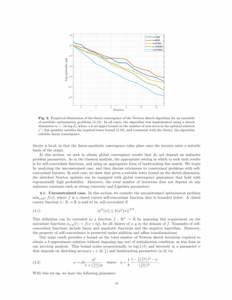
had at most s = ⌈2 log(d)⌉ non-zero entries. A calculation of the Gaussian width for this problem(see Appendix A for the details) shows that it suffices to take a sketch dimension m % s log d, andwe implemented the algorithm with this choice. Figure 2 shows the convergence rate of the Newtonsketch algorithm for the six different problem sizes: consistent with our theory, the sketch dimensionm≪ min{d, n} suffices to guarantee linear convergence in all cases.

It is also possible obtain an asymptotically super-linear rate by using an iteration-dependentsketching accuracy ǫ = ǫ(t). The following corollary summarizes one such possible guarantee:

Corollary 3.2. Consider the Newton sketch iterates using the iteration-dependent sketchingaccuracy ǫ(t) = 1

log(1+t) . Then with the same probability as in Theorem 3.1, we have

‖xt+1 − x∗‖2 ≤ 1

log(1 + t)

β

γ‖xt − x∗‖2 +

4L

γ‖xt − x∗‖22,

and consequently, super-linear convergence is obtained—namely, limt→∞‖xt+1−x∗‖2‖xt−x∗‖2 = 0.

Note that the price for this super-linear convergence is that the sketch size is inflated by the factorǫ−2(t) = log2(1 + t), so it is only logarithmic in the iteration number.

4. Newton sketch for self-concordant functions. The analysis and complexity estimatesgiven in the previous section involve the curvature constants (γ, β) and the Lipschitz constant L,which are seldom known in practice. Moreover, as with the analysis of classical Newton method, the

9

2 4 6 8 10 12

10-12

10-10

10-8

10-6

10-4

10-2

100

n=1000

n=8000

n=27000

n=125000

n=216000

Fig. 2. Empirical illustration of the linear convergence of the Newton sketch algorithm for an ensembleof portfolio optimization problems (3.13). In all cases, the algorithm was implemented using a sketchdimension m = ⌈4s log d⌉, where s is an upper bound on the number of non-zeros in the optimal solutionx∗; this quantity satisfies the required lower bound (3.10), and consistent with the theory, the algorithmexhibits linear convergence.

theory is local, in that the linear-quadratic convergence takes place once the iterates enter a suitablebasin of the origin.

In this section, we seek to obtain global convergence results that do not depend on unknownproblem parameters. As in the classical analysis, the appropriate setting in which to seek such resultsis for self-concordant functions, and using an appropriate form of backtracking line search. We beginby analyzing the unconstrained case, and then discuss extensions to constrained problems with self-concordant barriers. In each case, we show that given a suitable lower bound on the sketch dimension,the sketched Newton updates can be equipped with global convergence guarantees that hold withexponentially high probability. Moreover, the total number of iterations does not depend on anyunknown constants such as strong convexity and Lipschitz parameters.

4.1. Unconstrained case. In this section, we consider the unconstrained optimization problemminx∈Rd f(x), where f is a closed convex self-concordant function that is bounded below. A closedconvex function φ : R → R is said to be self-concordant if

|φ′′′(x)| ≤ 2 (φ′′(x))3/2

.(4.1)

This definition can be extended to a function f : Rd → R by imposing this requirement on the

univariate functions φx,y(t) : = f(x + ty), for all choices of x, y in the domain of f . Examples of self-concordant functions include linear and quadratic functions and the negative logarithm. Moreover,the property of self-concordance is preserved under addition and affine transformations.

Our main result provides a bound on the total number of Newton sketch iterations required toobtain a δ-approximate solution without imposing any sort of initialization condition, as was done inour previous analysis. This bound scales proportionally to log(1/δ) and inversely in a parameter νthat depends on sketching accuracy ǫ ∈ (0, 14 ) and backtracking parameters (a, b) via

ν = abη2

1 + ( 1+ǫ1−ǫ )ηwhere η =

1

8

1− 12 (

1+ǫ1−ǫ )

2 − a

( 1+ǫ1−ǫ )3

.(4.2)

With this set-up, we have the following guarantee:

10

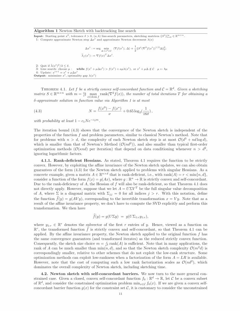
Algorithm 1 Newton Sketch with backtracking line search

Input: Starting point x0, tolerance δ > 0, (a, b) line-search parameters, sketching matrices {St}∞t=0 ∈ Rm×n.

1: Compute approximate Newton step ∆xt and approximate Newton decrement λ(x)

∆xt: = arg min

∆+xt∈C〈∇f(xt), ∆〉+ 1

2‖St(∇2

f(xt))

1/2∆‖22;

λf (xt) : = ∇f(x)T∆xt.

2: Quit if λ(xt)2/2 ≤ δ.3: Line search: choose µ : while f(xt + µ∆xt) > f(xt) + aµλ(xt), or xt + µ∆ /∈ C µ← bµ

4: Update: xt+1 = xt + µ∆xt

Output: minimizer xt, optimality gap λ(xt)

Theorem 4.1. Let f be a strictly convex self-concordant function and C = Rd. Given a sketching

matrix S ∈ Rm×n with m = c3

ǫ2 maxx∈dom f

rank(∇2f(x)), the number of total iterations T for obtaining a

δ-approximate solution in function value via Algorithm 1 is at most

N =f(x0)− f(x∗)

ν+ 0.65 log2(

1

16δ) ,(4.3)

with probability at least 1− c1Ne−c2m.

The iteration bound (4.3) shows that the convergence of the Newton sketch is independent of theproperties of the function f and problem parameters, similar to classical Newton’s method. Note thatfor problems with n > d, the complexity of each Newton sketch step is at most O(d3 + nd log d),which is smaller than that of Newton’s Method (O(nd2)), and also smaller than typical first-orderoptimization methods (O(κnd) per iteration) that depend on data conditioning whenever n > d2,ignoring logarithmic factors.

4.1.1. Rank-deficient Hessians. As stated, Theorem 4.1 requires the function to be strictlyconvex. However, by exploiting the affine invariance of the Newton sketch updates, we can also obtainguarantees of the form (4.3) for the Newton sketch applied to problems with singular Hessians. As aconcrete example, given a matrix A ∈ R

n×d that is rank-deficient, i.e., with rank(A) = r < min{n, d},consider a function of the form f(x) = g(Ax), where g : Rn → R is strictly convex and self-concordant.Due to the rank-deficiency of A, the Hessian of f will also be rank-deficient, so that Theorem 4.1 doesnot directly apply. However, suppose that we let A = UΣV T be the full singular value decompositionof A, where Σ is a diagonal matrix with Σjj = 0 for all indices j > r. With this notation, define

the function f(y) = g(AV y), corresponding to the invertible transformation x = V y. Note that as aresult of the affine invariance property, we don’t have to compute the SVD explicitly and perform thistransformation. We then have

f(y) = g(UΣy) = g(UΣ1:ry1:r),

where y1:r ∈ Rr denotes the subvector of the first r entries of y. Hence, viewed as a function on

Rr, the transformed function f is strictly convex and self-concordant, so that Theorem 4.1 can be

applied. By the affine invariance property, the Newton sketch applied to the original function f hasthe same convergence guarantees (and transformed iterates) as the reduced strictly convex function.Consequently, the sketch size choice m = c

ǫ2 rank(A) is sufficient. Note that in many applications, therank of A can be much smaller than min(n, d), and so that the Newton sketch complexity O(m2d) iscorrespondingly smaller, relative to other schemes that do not exploit the low-rank structure. Someoptimization methods can exploit low-rankness when a factorization of the form A = LR is available.However, note that the cost of computing such a low rank factorization scales as O(nd2), whichdominates the overall complexity of Newton sketch, including sketching time.

4.2. Newton sketch with self-concordant barriers. We now turn to the more general con-strained case. Given a closed, convex self-concordant function f0 : Rd → R, let C be a convex subsetof Rd, and consider the constrained optimization problem minx∈C f0(x). If we are given a convex self-concordant barrier function g(x) for the constraint set C, it is customary to consider the unconstrained

11

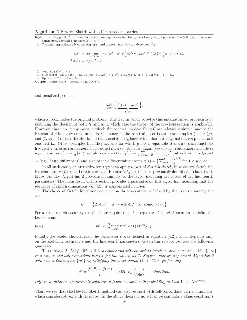
Algorithm 2 Newton Sketch with self-concordant barriers

Input: Starting point x0, constraint C, corresponding barrier function g such that f = f0+g, tolerance δ > 0, (α, β) line-search

parameters, sketching matrices St ∈ Rm×n.

1: Compute approximate Newton step ∆xt and approximate Newton decrement λf .

∆xt: = arg min

xt+∆∈C〈∇f(xt), ∆〉+ 1

2‖St(∇2

f0(xt))

1/2∆‖22 +

1

2∆T∇2

g(xt)∆;

λf (xt) : = ∇f(x)T∆xt

2: Quit if λ(xt)2/2 ≤ δ.3: Line search: choose µ : while f(xt + µ∆xt) > f(xt) + αµλ(xt), or xt + µ∆ /∈ C µ← βµ.

4: Update: xt+1 = xt + µ∆xt.Output: minimizer xt, optimality gap λ(xt).

and penalized problem

minx∈Rd

{f0(x) + g(x)︸ ︷︷ ︸

f(x)

},

which approximates the original problem. One way in which to solve this unconstrained problem is bysketching the Hessian of both f0 and g, in which case the theory of the previous section is applicable.However, there are many cases in which the constraints describing C are relatively simple, and so theHessian of g is highly-structured. For instance, if the constraint set is the usual simplex (i.e., x ≥ 0and 〈1, x〉 ≤ 1), then the Hessian of the associated log barrier function is a diagonal matrix plus a rankone matrix. Other examples include problems for which g has a separable structure; such functionsfrequently arise as regularizers for ill-posed inverse problems. Examples of such regularizers include ℓ2regularization g(x) = 1

2‖x‖22, graph regularization g(x) = 12

∑i,j∈E(xi − xj)

2 induced by an edge set

E (e.g., finite differences) and also other differentiable norms g(x) =(∑d

i=1 xpi

)1/p

for 1 < p <∞.

In all such cases, an attractive strategy is to apply a partial Newton sketch, in which we sketch theHessian term∇2f0(x) and retain the exact Hessian∇2g(x), as in the previously described updates (3.4).More formally, Algorithm 2 provides a summary of the steps, including the choice of the line searchparameters. The main result of this section provides a guarantee on this algorithm, assuming that thesequence of sketch dimensions {mt}∞t=0 is appropriately chosen.

The choice of sketch dimensions depends on the tangent cones defined by the iterates, namely thesets

Kt : ={∆ ∈ R

d | xt + α∆ ∈ C for some α > 0}.

For a given sketch accuracy ǫ ∈ (0, 1), we require that the sequence of sketch dimensions satisfies thelower bound

mt ≥ c3ǫ2

maxx∈C

W2(∇2f(x)1/2Kt).(4.4)

Finally, the reader should recall the parameter ν was defined in equation (4.2), which depends onlyon the sketching accuracy ǫ and the line search parameters. Given this set-up, we have the followingguarantee:

Theorem 4.2. Let f : Rd → R be a convex and self-concordant function, and let g : Rd → R ∪ {+∞}be a convex and self-concordant barrier for the convex set C. Suppose that we implement Algorithm 2with sketch dimensions {mt}t≥0 satisfying the lower bound (4.4). Then performing

N =f(x0)− f(x∗)

ν+ 0.65 log2

( 1

16δ

)iterations

suffices to obtain δ-approximate solution in function value with probability at least 1− c1Ne−c2m.

Thus, we see that the Newton Sketch method can also be used with self-concordant barrier functions,which considerably extends its scope. In the above theorem, note that we can isolate affine constraints

12

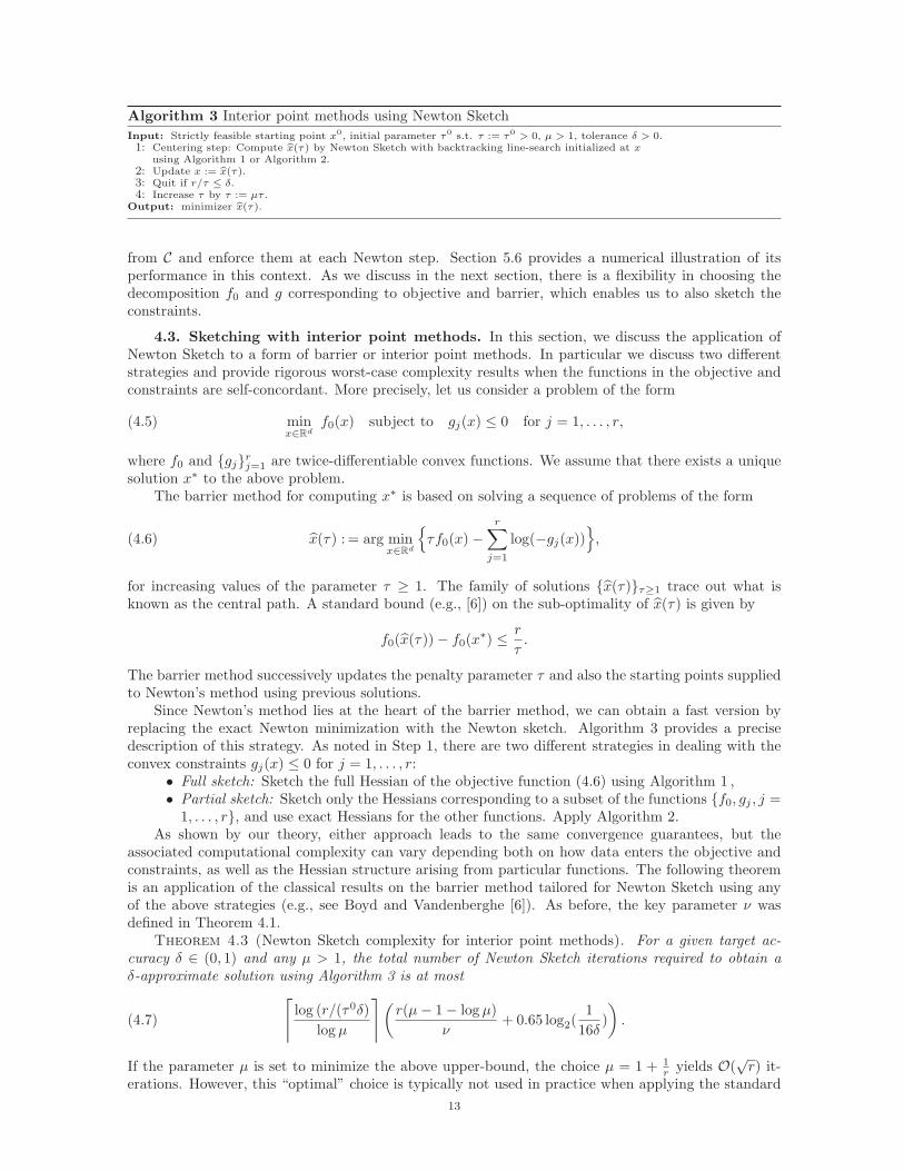
Algorithm 3 Interior point methods using Newton Sketch

Input: Strictly feasible starting point x0, initial parameter τ0 s.t. τ := τ0 > 0, µ > 1, tolerance δ > 0.1: Centering step: Compute x(τ) by Newton Sketch with backtracking line-search initialized at x

using Algorithm 1 or Algorithm 2.2: Update x := x(τ).3: Quit if r/τ ≤ δ.4: Increase τ by τ := µτ .

Output: minimizer x(τ).

from C and enforce them at each Newton step. Section 5.6 provides a numerical illustration of itsperformance in this context. As we discuss in the next section, there is a flexibility in choosing thedecomposition f0 and g corresponding to objective and barrier, which enables us to also sketch theconstraints.

4.3. Sketching with interior point methods. In this section, we discuss the application ofNewton Sketch to a form of barrier or interior point methods. In particular we discuss two differentstrategies and provide rigorous worst-case complexity results when the functions in the objective andconstraints are self-concordant. More precisely, let us consider a problem of the form

minx∈Rd

f0(x) subject to gj(x) ≤ 0 for j = 1, . . . , r,(4.5)

where f0 and {gj}rj=1 are twice-differentiable convex functions. We assume that there exists a uniquesolution x∗ to the above problem.

The barrier method for computing x∗ is based on solving a sequence of problems of the form

x(τ) : = arg minx∈Rd

{τf0(x)−

r∑

j=1

log(−gj(x))},(4.6)

for increasing values of the parameter τ ≥ 1. The family of solutions {x(τ)}τ≥1 trace out what isknown as the central path. A standard bound (e.g., [6]) on the sub-optimality of x(τ) is given by

f0(x(τ))− f0(x∗) ≤ r

τ.

The barrier method successively updates the penalty parameter τ and also the starting points suppliedto Newton’s method using previous solutions.

Since Newton’s method lies at the heart of the barrier method, we can obtain a fast version byreplacing the exact Newton minimization with the Newton sketch. Algorithm 3 provides a precisedescription of this strategy. As noted in Step 1, there are two different strategies in dealing with theconvex constraints gj(x) ≤ 0 for j = 1, . . . , r:

• Full sketch: Sketch the full Hessian of the objective function (4.6) using Algorithm 1 ,• Partial sketch: Sketch only the Hessians corresponding to a subset of the functions {f0, gj , j =

1, . . . , r}, and use exact Hessians for the other functions. Apply Algorithm 2.As shown by our theory, either approach leads to the same convergence guarantees, but the

associated computational complexity can vary depending both on how data enters the objective andconstraints, as well as the Hessian structure arising from particular functions. The following theoremis an application of the classical results on the barrier method tailored for Newton Sketch using anyof the above strategies (e.g., see Boyd and Vandenberghe [6]). As before, the key parameter ν wasdefined in Theorem 4.1.

Theorem 4.3 (Newton Sketch complexity for interior point methods). For a given target ac-curacy δ ∈ (0, 1) and any µ > 1, the total number of Newton Sketch iterations required to obtain aδ-approximate solution using Algorithm 3 is at most

⌈log (r/(τ0δ)

log µ

⌉(r(µ− 1− log µ)

ν+ 0.65 log2(

1

16δ)

).(4.7)

If the parameter µ is set to minimize the above upper-bound, the choice µ = 1 + 1r yields O(

√r) it-

erations. However, this “optimal” choice is typically not used in practice when applying the standard

13

Newton method; instead, it is common to use a fixed value of µ ∈ [2, 100]. In experiments, experiencesuggests that the number of Newton iterations needed is a constant independent of r and other param-eters. Theorem 4.3 allows us to obtain faster interior point solvers with rigorous worst-case complexityresults. We show different applications of Algorithm 3 in the following section.

5. Applications and numerical results. In this section, we discuss some applications of theNewton sketch to different optimization problems. In particular, we show various forms of Hessianstructure that arise in applications, and how the Newton sketch can be computed. When the objectiveand/or the constraints contain more than one term, the barrier method with Newton Sketch has someflexibility in sketching. We discuss the choices of partial Hessian sketching strategy in the barriermethod. It is also possible to apply the sketch in the primal or dual form, and we provide illustrationsof both strategies here.

5.1. Estimation in generalized linear models. Recall the problem of (constrained) maximumlikelihood estimation for a generalized linear model, as previously introduced in Example 2. It leadsto the family of optimization problems (3.7): here ψ : R → R is a given convex function arising fromthe probabilistic model, and C ⊆ R

d is a closed convex set that is used to enforce a certain type ofstructure in the solution. Popular choices of such constraints include ℓ1-balls (for enforcing sparsity in avector), nuclear norms (for enforcing low-rank structure in a matrix), and other non-differentiable semi-

norms based on total variation (e.g.,∑d−1j=1 |xj+1 − xj |), useful for enforcing smoothness or clustering

constraints.Suppose that we apply the Newton sketch algorithm to the optimization problem (3.7). Given the

current iterate xt, computing the next iterate xt+1 requires solving the constrained quadratic program

minx∈C

{1

2‖S diag

(ψ′′(〈ai, xt〉, yi)

)1/2A(x− xt)‖22 +

n∑

i=1

〈x, ψ′(〈ai, xt〉, yi)〉}.(5.1)

When the constraint C is a scaled version of the ℓ1-ball—that is, C = {x ∈ Rd | ‖x‖1 ≤ R} for some

radius R > 0—the convex program (5.1) is an instance of the Lasso program [36], for which there is avery large body of work. For small values of R, where the cardinality of the solution x is very small,an effective strategy is to apply a homotopy type algorithm, also known as LARS [15, 17], which solvesthe optimality conditions starting from R = 0. For other sets C, another popular choice is projectedgradient descent, which is efficient when projection onto C is computationally simple.

Focusing on the ℓ1-constrained case, let us consider the problem of choosing a suitable sketchdimension m. Our choice involves the ℓ1-restricted minimal eigenvalue of the data matrix ATA, whichis given by†

γ−s (A) : = min‖z‖2=1‖z‖1≤2

√s

‖Az‖22.(5.2)

Note that we are always guaranteed that γ−s (A) ≥ λmin(ATA). Our result also involves certain

quantities that depend on the function ψ, namely

ψ′′min : = minx∈C

mini=1,...,n

ψ′′(〈ai, x〉, yi), and ψ′′max : = maxx∈C

maxi=1,...,n

ψ′′(〈ai, x〉, yi),

where ai ∈ Rd is the ith row of A. With this set-up, supposing that the optimal solution x∗ has

cardinality at most ‖x∗‖0 ≤ s, then it can be shown (see Lemma A.1 in Appendix A) that it sufficesto take a sketch size

m = c0ψ′′max

ψ′′min

maxj=1,...,d

‖Aj‖22γ−s (A)

s log d,(5.3)

where c0 is a universal constant. Let us consider some examples to illustrate:• Least-Squares regression: ψ(u) = 1

2u2, ψ′′(u) = 1 and ψ′′min = ψ′′max = 1.

†Our choice of introducting the factor of two in the the constraint ‖z‖1 ≤ 2√s is for later theoretical convenience,

due to the structure of the tangent cone associated with the ℓ1-norm [31, 30].

14

• Poisson regression: ψ(u) = eu, ψ′′(u) = eu andψ′′

max

ψ′′min

= eRAmax

e−RAmin

• Logistic regression: ψ(u) = log(1 + eu), ψ′′(u) = eu

(eu+1)2 andψ′′

max

ψ′′min

= eRAmin

e−RAmax

(e−RAmax+1)2

(eRAmin+1)2,

where Amax : = maxi=1,...,n

‖ai‖∞, and Amin : = mini=1,...,n

‖ai‖∞.

For a large class of distributions of data matrices, the sketch size choice given in equation (5.3)scales as O(s log d). As an example, consider data matrices A ∈ R

n×d where each row is independentlysampled from a sub-Gaussian distribution with parameter one (see equation (2.3)). Then standardresults on random matrices [37] show that γ−s (A) > 1/2 with high probability as long as n > c1s log d for

a sufficiently large constant c1. In addition, we have maxj=1,...,d

‖Aj‖22 = O(n), as well asψ′′

max

ψ′′min

= O(log(n)).

For such problems, the per iteration complexity of Newton Sketch update scales as O(s2d log2(d)) usingstandard Lasso solvers (e.g., [20]) or as O(sd log(d)) using projected gradient descent, per gradientevaluation. Using ROS sketches and standard lasso interior point Lasso solvers to solve sketchedNewton updates, the total complexity is therefore (O(s2d log2(d)+nd log(d)) log(1/ǫ)). This scaling canbe substantially smaller than conventional algorithms that fail to exploit the small intrinsic dimensionof the tangent cone.

5.2. Semidefinite programs. The Newton sketch can also be applied to semidefinite programs.As one illustration, let us consider a metric learning problem studied in machine learning. Suppose thatwe are given d-dimensional feature vectors {ai}ni=1 and a collection of

(n2

)binary indicator variables

yij ∈ {−1,+1}n given by

yij =

{+1 if ai and aj belong to the same class

−1 otherwise,

defined for all distinct indices i, j ∈ {1, . . . , n}. The task is to estimate a positive semidefinite matrixX such that the semi-norm ‖(ai − aj)‖X : =

√〈ai − aj , X(ai − aj)〉 is a good predictor of whether or

not vectors i and j belong to the same class. Using the least-squares loss, one way in which to do sois by solving the semidefinite program (SDP)

minX�0

{ (n2)∑

i6=j

(〈X, (ai − aj)(ai − aj)

T 〉 − yij)2

+ λ trace(X)}.

Here the term trace(X), along with its multiplicative pre-factor λ > 0 that can be adjusted by theuser, is a regularization term for encouraging a relatively low-rank solution. Using the standard self-concordant barrier X 7→ log det(X) for the PSD cone, the barrier method involves solving a sequenceof sub-problems of the form

minX∈Rd×d

{τ

n∑

i=1

(〈X, aiaTi 〉 − yi)2 + τλ traceX − log det (X)

︸ ︷︷ ︸f(vec(X))

}.

Now the Hessian of the function vec(X) 7→ f(vec(X)) is a d2 × d2 matrix given by

∇2f(vec(X)

)= τ

(n2)∑

i6=jvec(Aij)vec(Aij)

T +X−1 ⊗X−1,

where Aij : = (ai−aj)(ai−aj)T . Then we can apply the barrier method with partial Hessian sketch onthe first term, {Sijvec(Aij)}i6=j and exact Hessian for the second term. Since the vectorized decision

variable is vec(X) ∈ Rd2 the complexity of Newton Sketch is O(m2d2) while the complexity of a

classical SDP interior-point solver is O(nd4) in practice.

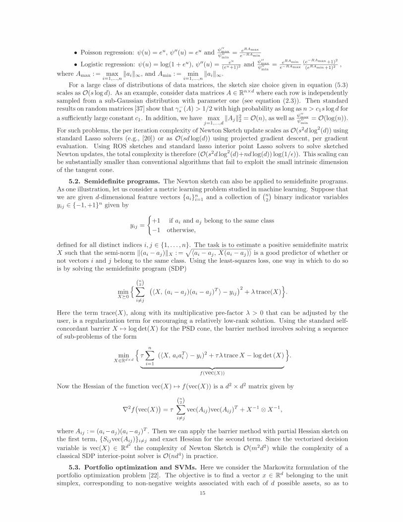
5.3. Portfolio optimization and SVMs. Here we consider the Markowitz formulation of theportfolio optimization problem [22]. The objective is to find a vector x ∈ R

d belonging to the unitsimplex, corresponding to non-negative weights associated with each of d possible assets, so as to

15

maximize the expected return minus a coefficient times the variance of the return. Letting µ ∈ Rd

denote a vector corresponding to mean return of the assets, and we let Σ ∈ Rd×d be a symmetric,

positive semidefinite matrix which represents the covariance of the returns. The optimization problemis given by

maxx≥0,

∑dj=1 xj≤1

{µTx− λ

1

2xTΣx

}.(5.4)

The covariance of returns is often estimated from past stock data via an empirical covariance matrixof the form Σ = ATA; here columns of A are time series corresponding to assets normalized by

√n,

where n is the length of the observation window.The barrier method can be used solve the above problem by solving penalized problems of the

form

minx∈Rd

{−τ µTx+ τλ

1

2xTATAx−

d∑

i=1

log(eTi x)− log(1− 1Tx)

︸ ︷︷ ︸f(x)

},

where ei ∈ Rd is the ith element of the canonical basis and 1 is a row vector of all-ones. Then the

Hessian of the above barrier penalized formulation can be written as

∇2f(x) = τλATA+(diag{x2i }di=1

)−1+ 11T .

Consequently, we can sketch the data dependent part of the Hessian via τλSA which has at most rankm and keep the remaining terms in the Hessian exact. Since the matrix 11T is rank one, the resultingsketched estimate is therefore diagonal plus rank (m + 1) where the matrix inversion lemma [16] canbe applied for efficient computation of the Newton Sketch update. Therefore, as long as m ≤ d,the complexity per iteration scales as O(md2), which is cheaper than the O(nd2) per step complexityassociated with classical interior point methods. We also note that support vector machine classificationproblems with squared hinge loss also has the same form as in equation (5.4), so that the same strategycan be applied.

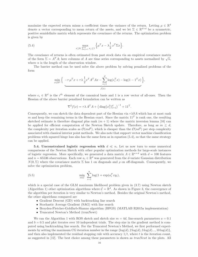
5.4. Unconstrained logistic regression with d ≪ n. Let us now turn to some numericalcomparisons of the Newton Sketch with other popular optimization methods for large-scale instancesof logistic regression. More specifically, we generated a data matrix A ∈ R

n×d with d = 100 featuresand n = 65536 observations. Each row ai ∈ R

d was generated from the d-variate Gaussian distributionN(0,Σ) where the covariance matrix Σ has 1 on diagonals and ρ on off-diagonals. Consequently, wesolve the optimization problem,

minx∈C

n∑

i=1

log(1 + exp(aTi xyi),(5.5)

which is a special case of the GLM maximum likelihood problem given in (3.7) using Newton sketch(Algorithm 1) other optimization algorithms where C = R

d. As shown in Figure 3, the convergence ofthe algorithm per iteration is very similar to Newton’s method. Besides the original Newton’s method,the other algorithms compared are

• Gradient Descent (GD) with backtracking line search• Stochastic Average Gradient (SAG) with line search• Broyden-Fletcher-Goldfarb-Shanno algorithm (BFGS) (MATLAB R2015a implementation)• Truncated Newton’s Method (trunNewt)

We ran the Algorithm 1 with ROS sketch and sketch size m = 4d, line-search parameters a = 0.1and b = 0.5 and plot iterates over 10 independent trials. The step size in the gradient method is com-puted using backtracking line search. For the Truncated Newton’s Method, we first performed experi-ments by setting the maximum CG iteration number in the range {log(d), 2 log(d), 3 log(d)..., 10 log(d)},and then also implemented the residual stopping rule with accuracy 1/t, where t is the iteration count,as suggested in [12]. The best choice among these parameters is shown as trunNewt in the plots. All

16

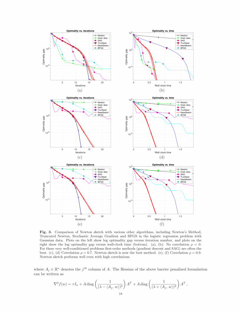
algorithms are implemented in MATLAB (R2015a). In the plots, each iteration of the SAG algorithmcorresponds to a pass over the data, which is of comparable complexity to a single iteration of GD.In order to keep the plots relatively uncluttered, we have excluded Stochastic Gradient Descent sinceit is dominated by another stochastic first-order method (SAG), and Accelerated Gradient Method[26] as it is quite similar to Gradient Descent. Plots on the left in Figure 3—that is panels (a), (c)and (e)—show the log duality gap versus the number of iterations: as expected, on this scale, theclassical form of Newton’s method is the fastest. However, when the log optimality gap is plottedversus the wall-clock time (right-side panels (b), (d) and (e)), we now see that the Newton sketch isthe fastest. The panels (a) and (b) exhibit the case when there is no correlation (ρ = 0). For thesevery well-conditioned problems first-order methods are often the best. However, panels (c) and (d)exhibit the case when correlation is moderate (ρ = 0.5) where it can be seen that Newton sketch is thefastest method. Panels (e) and (f) further demonstrates that Newton sketch performs well even withhigh correlations (ρ = 0.9).

On the other hand, Figure 4 reveals the sensitivity of first order and stochastic gradient typemethods to the distribution of the covariates. For these experiments, we generated a feature matrixA with d = 100 features and n = 65536 observations where each row ai ∈ R

d was generated fromthe Student’s t-distribution with covariance Σ. The covariance matrix Σ has 1 on the diagonal andρ off the diagonal. The distribution of the data rows generated from Student’s t-distribution is moreheavy-tailed compared to a normal distribution. As it can be seen in Figure 3, SAG and GD performquite poor compared to Figure 3 under the heavy-tailed distribution even in the uncorrelated case(ρ = 0). However, the performance of the Newton sketch is not changed by the distribution or theconditioning of the data and so outperforms other methods as predicted by our theory.

5.5. ℓ1-constrained logistic regression and data conditioning. Next we provide some nu-merical comparisons of Newton Sketch, Newton’s Method and Projected Gradient Descent when ap-plied to an ℓ1-constrained form of logistic regression. We consider the optimization problem (5.5)where the constraint set C is a scaled ℓ1 ball. More specifically, we first generate a feature matrixA ∈ R

n×d based on d = 100 features and n = 1000 observations. Each row ai ∈ Rd is drawn from the

d-variate Gaussian distribution N(0,Σ); the covariance matrix has entries of the form Σij = 2|ρ|i−j ,where ρ ∈ [0, 1) is a parameter controlling the correlation, and hence the condition number of thedata. For 10 different values of ρ we solved the ℓ1-constrained problem (‖x‖1 ≤ 0.1), performing 200independent trials (regenerating the data and sketching matrices randomly each time). The Newtonand sketched Newton steps (Algorithm 1) are solved exactly using the homotopy algorithm—that is,the Lasso modification of the LARS updates [29, 15] using a Matlab implementation [34]. The homo-topy method is very effective when the solution is very sparse. The ROS sketch with a sketch size ofm = ⌈4 × 10 log d⌉ is used where 10 is the estimated cardinality of solution. As shown in Figure 5,Newton Sketch converges in about 6 (± 2) iterations independent of data conditioning while the ex-act Newton’s method converges in 3 (± 1) iterations. However the number of iterations needed forprojected gradient with line search increases steeply as ρ increases. Note that, ignoring logarithmicterms, the projected gradient and Newton Sketch have similar computational complexity (O(nd)) periteration while the Newton’s method has higher computational complexity (O(nd2)).

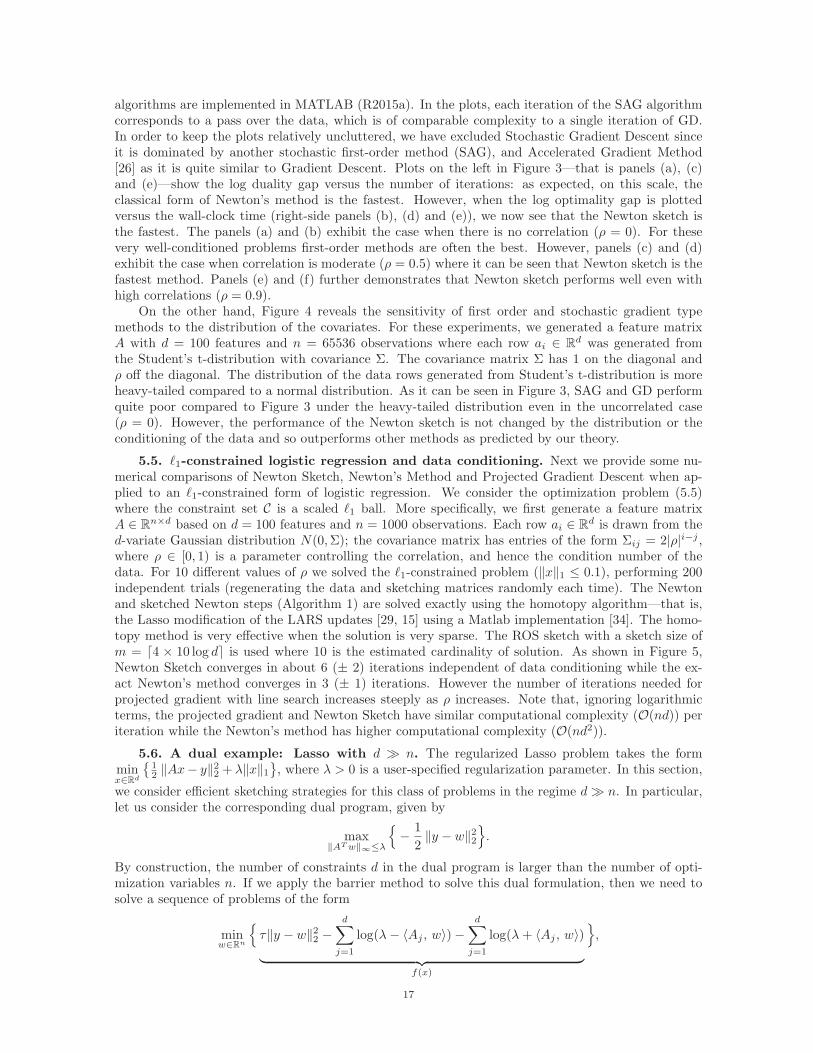
5.6. A dual example: Lasso with d ≫ n. The regularized Lasso problem takes the formminx∈Rd

{12 ‖Ax− y‖22 + λ‖x‖1

}, where λ > 0 is a user-specified regularization parameter. In this section,

we consider efficient sketching strategies for this class of problems in the regime d≫ n. In particular,let us consider the corresponding dual program, given by

max‖ATw‖∞≤λ

{− 1

2‖y − w‖22

}.

By construction, the number of constraints d in the dual program is larger than the number of opti-mization variables n. If we apply the barrier method to solve this dual formulation, then we need tosolve a sequence of problems of the form

minw∈Rn

{τ‖y − w‖22 −

d∑

j=1

log(λ− 〈Aj , w〉)−d∑

j=1

log(λ+ 〈Aj , w〉)︸ ︷︷ ︸

f(x)

},

17

5 10 15 20

Iterations

10-5

100

Optim

alit

y g

ap

Optimality vs. iterations

Newton

Grad. desc

SAG

TrunNewt

NewtSketch

BFGS

0 0.5 1 1.5

Wall clock time

10-5

100

105

Optim

alit

y g

ap

Optimality vs. time

Newton

Grad. desc

SAG

TrunNewt

NewtSketch

BFGS

(a) (b)

5 10 15 20

Iterations

10-5

100

Optim

alit

y g

ap

Optimality vs. iterations

Newton

Grad. desc

SAG

TrunNewt

NewtSketch

BFGS

0 0.5 1 1.5

Wall clock time

10-5

100

105

Optim

alit

y g

ap

Optimality vs. time

Newton

Grad. desc

SAG

TrunNewt

NewtSketch

BFGS

(c) (d)

5 10 15 20

Iterations

10-5

100

Optim

alit

y g

ap

Optimality vs. iterations

Newton

Grad. desc

SAG

TrunNewt

NewtSketch

BFGS

0 0.5 1 1.5

Wall clock time

10-5

100

105

Optim

alit

y g

ap

Optimality vs. time

Newton

Grad. desc

SAG

TrunNewt

NewtSketch

BFGS

(e) (f)

Fig. 3. Comparison of Newton sketch with various other algorithms, including Newton’s Method,Truncated Newton, Stochastic Average Gradient and BFGS in the logistic regression problem withGaussian data. Plots on the left show log optimality gap versus iteration number, and plots on theright show the log optimality gap versus wall-clock time (bottom). (a), (b): No correlation ρ = 0.For these very well-conditioned problems first-order methods (gradient descent and SAG) are often thebest. (c), (d) Correlation ρ = 0.7. Newton sketch is now the best method. (e), (f) Correlation ρ = 0.9.Newton sketch performs well even with high correlations.

where Aj ∈ Rn denotes the jth column of A. The Hessian of the above barrier penalized formulation

can be written as

∇2f(w) = τIn +Adiag

(1

(λ− 〈Aj , w〉)2)AT +Adiag

(1

(λ+ 〈Aj , w〉)2)AT ,

18

5 10 15 20

Iterations

10-5

100

Optim

alit

y g

ap

Optimality vs. iterations

Newton

Grad. desc

SAG

TrunNewt

NewtSketch

BFGS

0 0.5 1 1.5

Wall clock time

10-5

100

105

Optim

alit

y g

ap

Optimality vs. time

Newton

Grad. desc

SAG

TrunNewt

NewtSketch

BFGS

(a) (b)

5 10 15 20

Iterations

10-5

100

Optim

alit

y g

ap

Optimality vs. iterations

Newton

Grad. desc

SAG

TrunNewt

NewtSketch

BFGS

0 0.5 1 1.5

Wall clock time

10-5

100

105

Optim

alit

y g

ap

Optimality vs. time

Newton

Grad. desc

SAG

TrunNewt

NewtSketch

BFGS

(c) (d)

5 10 15 20

Iterations

10-5

100

Optim

alit

y g

ap

Optimality vs. iterations

Newton

Grad. desc

SAG

TrunNewt

NewtSketch

BFGS

0 0.5 1 1.5

Wall clock time

10-5

100

105

Optim

alit

y g

ap

Optimality vs. time

Newton

Grad. desc

SAG

TrunNewt

NewtSketch

BFGS

(e) (f)

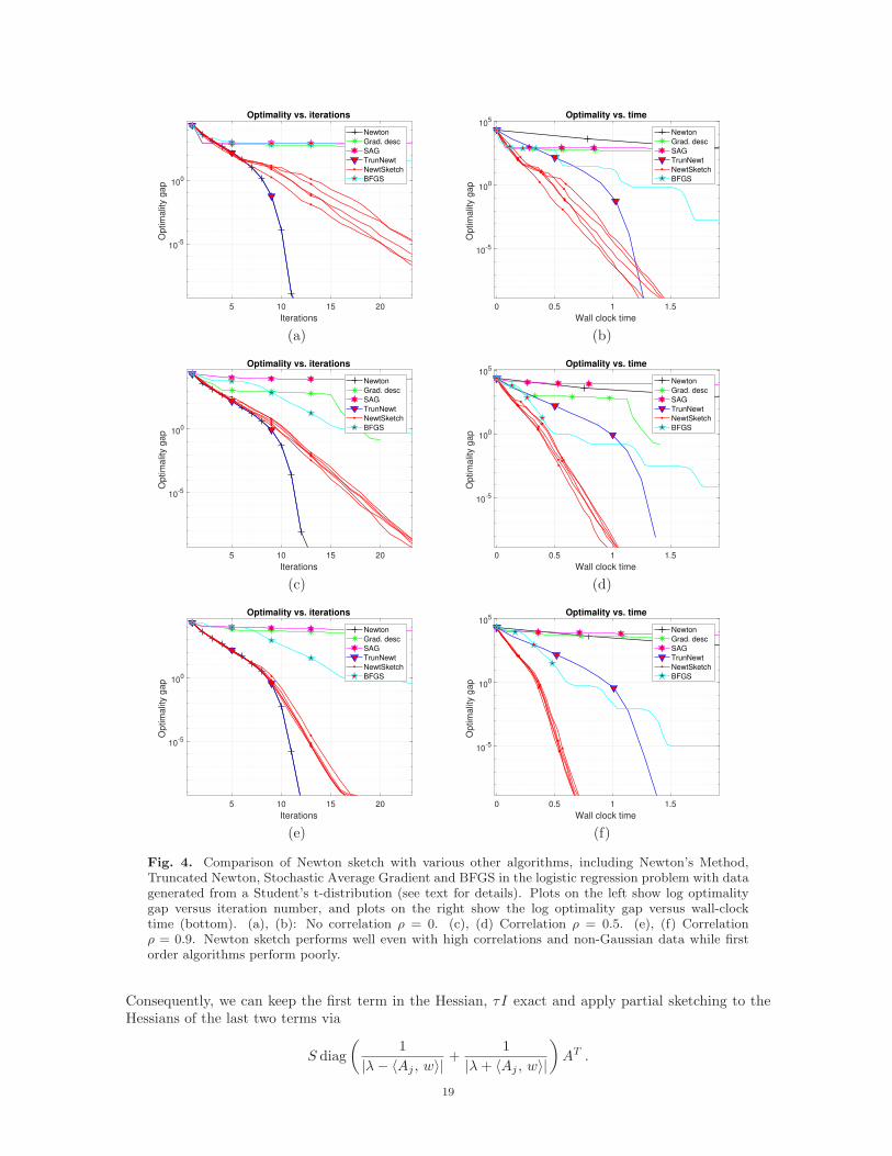
Fig. 4. Comparison of Newton sketch with various other algorithms, including Newton’s Method,Truncated Newton, Stochastic Average Gradient and BFGS in the logistic regression problem with datagenerated from a Student’s t-distribution (see text for details). Plots on the left show log optimalitygap versus iteration number, and plots on the right show the log optimality gap versus wall-clocktime (bottom). (a), (b): No correlation ρ = 0. (c), (d) Correlation ρ = 0.5. (e), (f) Correlationρ = 0.9. Newton sketch performs well even with high correlations and non-Gaussian data while firstorder algorithms perform poorly.

Consequently, we can keep the first term in the Hessian, τI exact and apply partial sketching to theHessians of the last two terms via

S diag

(1

|λ− 〈Aj , w〉|+

1

|λ+ 〈Aj , w〉|

)AT .

19

0 0.1 0.2 0.3 0.4 0.5 0.6 0.7 0.80

20

40

60

80

100

120

140

160

180

200

Correlation ρ

Nu

mb

er

of

ite

ratio

ns

Iterations vs Conditioning

Original Newton

Newton Sketch

Projected Gradient

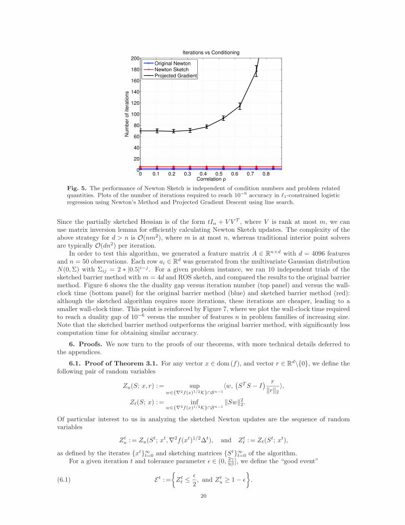
Fig. 5. The performance of Newton Sketch is independent of condition numbers and problem relatedquantities. Plots of the number of iterations required to reach 10−6 accuracy in ℓ1-constrained logisticregression using Newton’s Method and Projected Gradient Descent using line search.

Since the partially sketched Hessian is of the form tIn + V V T , where V is rank at most m, we canuse matrix inversion lemma for efficiently calculating Newton Sketch updates. The complexity of theabove strategy for d > n is O(nm2), where m is at most n, whereas traditional interior point solversare typically O(dn2) per iteration.

In order to test this algorithm, we generated a feature matrix A ∈ Rn×d with d = 4096 features

and n = 50 observations. Each row ai ∈ Rd was generated from the multivariate Gaussian distribution

N(0,Σ) with Σij = 2 ∗ |0.5|i−j . For a given problem instance, we ran 10 independent trials of thesketched barrier method with m = 4d and ROS sketch, and compared the results to the original barriermethod. Figure 6 shows the the duality gap versus iteration number (top panel) and versus the wall-clock time (bottom panel) for the original barrier method (blue) and sketched barrier method (red):although the sketched algorithm requires more iterations, these iterations are cheaper, leading to asmaller wall-clock time. This point is reinforced by Figure 7, where we plot the wall-clock time requiredto reach a duality gap of 10−6 versus the number of features n in problem families of increasing size.Note that the sketched barrier method outperforms the original barrier method, with significantly lesscomputation time for obtaining similar accuracy.

6. Proofs. We now turn to the proofs of our theorems, with more technical details deferred tothe appendices.

6.1. Proof of Theorem 3.1. For any vector x ∈ dom (f), and vector r ∈ Rd\{0}, we define the

following pair of random variables

Zu(S; x, r) : = supw∈{∇2f(x)1/2K}∩Sn−1

〈w,(STS − I

) r

‖r‖2〉,

Zℓ(S; x) : = infw∈{∇2f(x)1/2K}∩Sn−1

‖Sw‖22.

Of particular interest to us in analyzing the sketched Newton updates are the sequence of randomvariables

Ztu : = Zu(St; xt,∇2f(xt)1/2∆t), and Ztℓ : = Zℓ(S

t; xt),

as defined by the iterates {xt}∞t=0 and sketching matrices {St}∞t=0 of the algorithm.For a given iteration t and tolerance parameter ǫ ∈ (0, 2γ9β ], we define the “good event”

Et : ={Ztℓ ≤

ǫ

2, and Ztu ≥ 1− ǫ

}.(6.1)

20

number of Newton iterations

0 500 1000 1500

duality

gap

100

Original Newton

Newton Sketch

wall-clock time (seconds)

5 10 15 20 25 30 35 40 45

dualit

y g

ap

10-10

100

Fig. 6. Plots of the duality gap versus iteration number (top panel) and duality gap versus wall-clocktime (bottom panel) for the original barrier method (blue) and sketched barrier method (red). Thesketched interior point method is run 10 times independently yielding slightly different curves in red.While the sketched method requires more iterations, its overall wall-clock time is much smaller.

dimension n

1,000 2000 10,000 50000 100,000

wa

ll-clo

ck t

ime

(se

co

nd

s)

0

100

200

300

400

500

Wall-clock time for obtaining accuract 1E-6

Exact Newton

Newton's Sketch

Fig. 7. Plot of the wall-clock time in seconds for reaching a duality gap of 10−6 for the standard andsketched interior point methods as n increases (in log-scale). The sketched interior point method hassignificantly lower computation time compared to the original method.

Given these two definitions, the proof of the theorem is based on two auxiliary lemmas, the firstof which establishes a key recursion on the error in the algorithm:

Lemma 6.1 (Key recursion). Suppose that the event ∩Nt=1Et holds. Then given any initializationx0 such that ‖x0 − x∗‖2 ≤ γ

8L , the error vectors ∆t = xt − x∗ satisfy the recursion

‖∆t+1‖2 ≤ ZtuZtℓ

β

7γ‖∆t‖2 +

1

Ztℓ

8L

7γ‖∆t‖22 for all t = 0, 1, . . . , N − 1.(6.2)

21

Note that since we haveZtuZtℓ

≤ ǫ and 1Ztℓ

≤ 2 whenever the event ∩Nt=1Et holds, the bound (3.11) stated

in the theorem then follows.In order to complete the proof, we need to establish that the event ∩Nt=1Et holds with the stated

probability. The following result gives sufficient conditions on the sketch dimension for such a guaranteeto hold:

Lemma 6.2 (Sufficient conditions on sketch dimension [31]).(a) For sub-Gaussian sketch matrices, given a sketch size m > c0

ǫ2 maxx∈CW2(∇2f(x)1/2K), we have

P[Et] ≥ 1− c1e

−c2mǫ2 .(6.3)

(b) For randomized orthogonal system (ROS) sketches and JL embeddings, over the class of self-

bounding cones, given a sketch size m > c0 log4 nǫ2 maxx∈CW2(∇2f(x)1/2K), we have

P[Et] ≥ 1− c1e

−c2 mǫ2

log4 n .(6.4)

Together with Lemma 6.1, the claim of the theorem follows.

It remains to prove Lemma 6.1, and the bulk of our effort is devoted to this task.

Proof of Lemma 6.1: We prove the recursion (6.2) by exploiting the convex optimality conditionsthat define the iterates xt+1 and the optimum x∗. Recall the function x 7→ Φ(x;St) that underliesthe sketch Newton update (3.2) in moving from iterate xt to iterate xt+1. Since the vectors xt+1 andx∗ are optimal and feasible, respectively, for the constrained optimization problem, the error vector∆t+1 : = xt+1 − x∗ satisfies the inequality 〈∇Φ(xt+1;St), −∆t+1〉 ≥ 0, or equivalently

〈(St∇2f(xt)1/2)TSt∇2f(xt)1/2(∆t+1 −∆t) +∇f(xt), −∆t+1〉 ≥ 0.

Similarly, since x∗ and xt+1 are optimal and feasible, respectively, for the minimization of f , we have

〈f(x∗), ∆t+1〉 ≥ 0.

Adding these two inequalities and re-arranging leads to the basic inequality

‖St∇2f(xt)1/2∆t+1‖22︸ ︷︷ ︸LHS

≤ 〈St∇2f(xt)1/2∆t+1, St∇2f(xt)1/2∆t〉 − 〈∇f(xt)−∇f(x∗), ∆t+1〉︸ ︷︷ ︸RHS

(6.5)

This inequality forms the core of our argument: in particular, the next steps in our proof are devotedto establishing the following bounds on the left-hand and right-hand sides:

LHS ≥ Ztℓ

{γ − L‖∆t‖2

}‖∆t+1‖22, and(6.6a)

RHS ≤ Ztu

{β + L‖∆t‖2

}‖∆t‖2‖∆t+1‖2 + L‖∆t‖22‖∆t+1‖2.(6.6b)

Taking these bounds as given for the moment, let us complete the proof of the recursion (6.2). Ourproof consists of two steps:• we first show that bound (6.2) holds for ∆t+1 whenever ‖∆t‖2 ≤ γ

8L .• we then show by induction that, conditioned on the event ∩Nt=1Et, the bound ‖∆t‖2 ≤ γ

8L holds forall iterations t = 0, 1, . . . , N .

Assuming that ‖∆t‖2 ≤ γ8L , then our basic inequality (6.5) combined with the bounds (6.6) implies

that

‖∆t+1‖2 ≤ Ztu{β + L‖∆t‖2}Ztℓ{γ − L‖∆t‖2}

‖∆t‖2 +L

Ztℓ{γ − L‖∆t‖2}‖∆t‖22.

We have L‖∆t‖2 ≤ γ/8 ≤ β/8, and (γ − L‖∆t‖2)−1 ≤ 87γ hence

‖∆t+1‖2 ≤ ZtuZtℓ

9

7

β

γ‖∆t‖2 +

1

Ztℓ

8L

7γ‖∆t‖22,(6.7)

22

thereby verifying the claim (6.2).Now we need to check for any iteration t, the bound ‖∆t‖2 ≤ γ

8L holds. We do so by induction.The base case is trivial since ‖∆0‖2 ≤ γ

8L by assumption. Supposing that the bound holds at time t,by our argument above, inequality (6.7) holds, and hence

‖∆t+1‖2 ≤ 9

56

βZtuLZtℓ

+16L

7γZtℓ

γ2

64L2=

ZtuZtℓ

9

28

β

L+

1

Ztℓ

1

28

γ

L.

Whenever Et holds, we haveZtuZtℓ

≤ 2γ9β and 1

Ztℓ≤ 1

2 , whence ‖∆t+1‖2 ≤(

128 + 1

14

)γL ≤ γ

8L , as claimed.

The final remaining detail is to prove the bounds (6.6).

Proof of the lower bound (6.6a). We first prove the lower bound (6.6a) on the LHS. Since∇2f(xt)1/2∆t+1 ∈ ∇2f(xt)1/2K, the definition of Ztℓ ensures that

LHS = ‖St∇2f(xt)1/2∆t+1‖22 ≥ Ztℓ‖∇2f(xt)1/2∆t+1‖22(i)= Ztℓ(∆

t+1)T∇2f(xt)∆t+1

= Ztℓ{(∆t+1)T∇2f(x∗)∆t+1 + (∆t+1)T (∇2f(xt)−∇2f(x∗))∆t+1

(ii)

≥ Ztℓ{γ‖∆t+1‖22 − L‖∆t+1‖22‖∆t‖2

}

where step (i) follows since (∇2f(x)1/2)T∇2f(x)1/2 = ∇2f(x), and step (ii) follows from the definitionsof γ and L.

Proof of the upper bound (6.6b). Next we prove the upper bound (6.6b) on the RHS. Throughoutthis proof, we write S instead of St so as to simplify notation. By the integral form of Taylor series,we have

RHS =

∫ 1

0

(∆t)T[(S∇2f(xt)1/2)TS∇2f(xt)1/2 −∇2f(xt + u(x∗ − xt))

]∆t+1du

= T1 + T2

where

T1 : = (∆t)T[(S∇2f(xt)1/2)TS∇2f(xt)1/2 −∇2f(xt)

]∆t+1, and(6.8a)

T2 : =

∫ 1

0

(∆t)T[−∇2f(xt + u(x∗ − xt)) +∇2f(xt)

]∆t+1du.(6.8b)

Here the decomposition into T1 and T2 follows by adding and subtracting the term (∆t)T∇2f(xt)∆t+1.We begin by upper bounding the term T1. By the definition of Ztu, we have

T1 ≤∣∣∣∣(∆

t)TQT (xt)

[STS

m− I

]∇2f(xt)1/2∆t+1

∣∣∣∣ ≤ Z2‖∇2f(xt)1/2∆t‖2‖∇2f(xt)1/2∆t+1‖2.

By adding and subtracting terms, we have

‖∇2f(xt)1/2∆t‖22 = (∆t)T∇2f(xt)∆t = (∆t)T∇2f(x∗)∆t + (∆t)T[∇2f(xt)−∇2f(x∗)

]∆t

≤ β‖∆t‖22 + L‖∆t‖3 = ‖∆t‖22(β + L‖∆t‖),

where the final step follows from the definitions of β and L, as bounds on the Hessian, and its Lipschitzconstant, respectively. A similar argument yields

‖∇2f(xt)1/2∆t+1‖22 ≤ ‖∆t+1‖22(β + L‖∆t‖).

Overall, we have shown that

T1 ≤ Ztu(β + L‖∆t‖)‖∆t‖2‖∆t+1‖2.(6.9)

23

Turning to the quantity T2, we have

T2 ≤{∫ 1

0

supv,v∈K∩Sd−1

∣∣vT[∇2f(xt + u(x∗ − xt))−∇2f(xt)

]v∣∣ du

}‖∆t‖2‖∆t+1‖2

≤ L‖∆t‖22‖∆t+1‖2,(6.10)

where the final step uses the local Lipschitz property again. Combining the bound (6.9) with thebound (6.10) yields the bound (6.6b) on the RHS.

6.2. Proof of Theorem 4.1. Recall that in this case, we assume that f is a self-concordantand strictly convex function. We adopt the following notation and conventions from Nesterov andNemirovski [28]. For a given vector x ∈ R

d, we define the pair of dual norms

‖u‖x : = 〈∇2f(x)u, u〉1/2, and ‖v‖∗x : = 〈∇2f(x)−1v, v〉1/2 ,

as well as the Newton decrement

λf (x) = 〈∇2f(x)−1∇f(x), ∇f(x)〉1/2 = ‖∇2f(x)−1∇f(x)‖x = ‖∇2f(x)−1/2∇f(x)‖2 .

Note that ∇2f(x)−1 is well-defined for strictly convex self-concordant functions. In terms of thisnotation, the exact Newton update is given by x 7→ xNE : = x+ vNE, where

vNE : = arg minz∈C−x

{ 1

2‖∇2f(x)1/2z‖22 + 〈z, ∇f(x)〉

︸ ︷︷ ︸Φ(z)

}.(6.11a)

On the other hand, the Newton sketch update is given by x 7→ xNSK : = x+ vNSK, where

vNSK : = arg minz∈C−x

{1

2‖S∇2f(x)1/2z‖22 + 〈z, ∇f(x)〉

}.(6.11b)

The proof of Theorem 4.1 given in this section involves the unconstrained case (C = Rd), whereas the

proofs of later theorems involve the more general constrained case. In the unconstrained case, the twoupdates take the simpler forms

xNE = x− (∇2f(x))−1∇f(x), and xNSK = x− (∇2f(x)1/2STS∇2f(x)1/2)−1∇f(x).

Let us make a few high-level remarks about the structure of the proof. For a self-concordantfunction, the sub-optimality of the Newton iterate xNE in function value satisfies the bound

f(xNE)− minx∈Rd

f(x)

︸ ︷︷ ︸f(x∗)

≤[λf (xNE)

]2.

This classical bound is not directly applicable to the Newton sketch update, since it involves the approx-imate Newton decrement λf (x)

2 = −〈∇f(x), vNSK〉, as opposed to the exact one λf (x)2 = −〈∇f(x), vNE〉.

Thus, our strategy is to prove that with high probability over the randomness in the sketch matrix,the approximate Newton decrement can be used as an exit condition.

Our argument for doing so consists of two main parts. First, we show that under appropriateconditions on the random sketch, the approximate and exact Newton updates are guaranteed to berelatively close. Second, in analogy to the analysis of classical Newton’s method, we analyze thesketched Newton algorithm in two phases, depending on whether the sketched Newton decrementλf (x) is strictly greater than or less than or equal to η.

6.2.1. Relating the sketched and exact Newton directions. Recalling the definitions (6.11a)and (6.11b) of the exact vNE and sketched Newton vNSK update directions, our first step is to show thatunder suitable conditions on the random sketch, these two directions are close with high probability.Recall the definition (3.8) of the tangent cone K of the set C at a given vector x ∈ C. With this

24

notation, the following lemma provides a high probability bound on these two directions:

Lemma 6.3. Let S ∈ Rm×n be a sub-Gaussian, ROS or JL sketching matrix and consider any

fixed vector x ∈ C independent of the sketch matrix. If m ≥ c0W(∇2f(x)1/2K)2

ǫ2 , then

∥∥∥∇2f(x)1/2(vNSK − vNE)∥∥∥2≤ ǫ

∥∥∥∇2f(x)1/2vNE

∥∥∥2

(6.12)

with probability at least 1− c1e−c2mǫ2 .

Proof. The proof follows similar lines to the proof of Theorem 3.1, in particular exploiting theconvex optimality conditions that define the exact and sketched Newton updates. Let u be a unit-normvector independent of S, and consider the random quantities

Zℓ(S, x) : = infv∈∇2f(x)1/2Kt∩Sn−1

‖Sv‖22 and(6.13a)

Zu(S, x) : = supv∈∇2f(x)1/2Kt∩Sn−1

∣∣∣〈u, (STS − In) v〉∣∣∣.(6.13b)

By the optimality and feasibility of vNSK and vNE (respectively) for the sketched Newton update (6.11b),we have

1

2‖S∇2f(x)1/2vNSK‖22 − 〈vNSK, ∇f(x)〉 ≤

1

2‖∇2f(x)1/2vNE‖22 − 〈vNE, ∇f(x)〉.

Defining the difference vector e : = vNSK − vNE, some algebra leads to the basic inequality

1

2‖S∇2f(x)1/2e‖22 ≤ −〈∇2f(x)1/2vNE, S

TS∇2f(x)1/2e〉+ 〈e, ∇f(x)〉.(6.14)

Moreover, by the optimality and feasibility of vNE and vNSK for the exact Newton update (6.11a), wehave

〈∇2f(x)vNE −∇f(x), e〉 = 〈∇2f(x)vNE −∇f(x), vNSK − vNE〉 ≥ 0.(6.15)

Consequently, by adding and subtracting 〈∇2f(x)vNE, e〉, we find that

1

2‖S∇2f(x)1/2e‖22 ≤

∣∣∣〈∇2f(x)1/2vNE,(In − STS

)∇2f(x)1/2e〉

∣∣∣ .(6.16)

By definition, the error vector e belongs to the cone Kt and the vector ∇2f(x)1/2vNE is fixed andindependent of the sketch. Consequently, invoking definitions (6.13a) and (6.13b) of the randomvariables Zℓ and Zu yields

1

2‖S∇2f(x)1/2e‖22 ≥ Zℓ

2‖∇2f(x)1/2e‖22,

∣∣∣〈∇2f(x)1/2vNE,(In − STS

)∇2f(x)1/2e〉

∣∣∣ ≤ Zu‖∇2f(x)1/2vNE‖2 ‖∇2f(x)1/2e‖2,

Putting together the pieces, we find that

∥∥∥∇2f(x)1/2(vNSK − vNE)∥∥∥2≤ 2Zu(S, x)

Zℓ(S, x)

∥∥∥∇2f(x)1/2(vNE)∥∥∥2.(6.17)

Finally, for any δ ∈ (0, 1), let us define the event E(δ) = {Zℓ ≥ 1−δ, and Zu ≤ δ}. By Lemma 4 and

Lemma 5 from our previous paper [31], we are guaranteed that P[E(δ)] ≥ 1− c1e−c2mδ2 . Conditioned

on the event E(δ), the bound (6.17) implies that

∥∥∥∇2f(x)1/2(vNSK − vNE)∥∥∥2≤ 2δ

1− δ

∥∥∥∇2f(x)1/2(vNE)∥∥∥2.

By setting δ = ǫ4 , the claim follows.

25

6.2.2. Two phase analysis. Similar to the standard analysis of Newton’s method, our next stepin the analysis of the Newton sketch algorithm is to consider two different phases, as defined by themagnitude of the decrement λf (x):

• First phase: Decrement λf (x) > η.

• Second phase: Decrement λf (x) ≤ η.

In each phase, we establish different guarantees on the behavior of the sketched update xNSK based ona starting vector x.

Lemma 6.4. For ǫ ∈ (0, 1/2), there exist constants ν > 0 and η ∈ (0, 1/16) such that:

(a) If λf (x) > η, then f(xNSK)− f(x) ≤ −ν with probability at least 1− c1e−c2mǫ2 .

(b) Conversely, if λf (x) ≤ η, then

λf (xNSK) ≤ λf (x), and(6.18a)

λf (xNSK) ≤(1625

)λf (x),(6.18b)

where both bounds hold with probability 1− c1ec2mǫ

2

.

Using this lemma, let us now complete the proof of the theorem, dividing our analysis into the twophases of the algorithm.

First phase analysis: Lemma 6.4(a) ensures that each iteration in the first phase decreases thefunction value by at least ν > 0; consequently, the number of first phase iterations N1 is at most

N1 : =f(x0)− f(x∗)

ν,

with probability at least 1−N1c1e−c2m.

Second phase analysis: Next, let us suppose that at some iteration t, the condition λf (xt) ≤ η

holds, so that part (b) of Lemma 6.4 can be applied. In fact, the bound (6.18a) then guarantees that

λf (xt+1) ≤ η, so that we may apply the contraction bound (6.18b) repeatedly for N2 rounds so as to

obtain that

λf (xt+N2) ≤

(1625

)N2λf (x

t)

with probability 1−N2c1ec2m.

Since λf (xt) ≤ η ≤ 1/16 by assumption, the self-concordance of f then implies that

f(xt+k)− f(x∗) ≤(16

25

)k1

16.

Therefore, in order to ensure that and consequently for achieving f(xt+k) − f(x∗) ≤ ǫ, it suffices forthe number of second phase iterations to be lower bounded as N2 ≥ 0.65 log2(

116ǫ ).

Putting together the two phases, we conclude that the total number of iterations N required toachieve ǫ- accuracy is at most

N = N1 +N2 ≤ f(x0)− f(x∗)

γ+ 0.65 log2(

1

16ǫ) ,

and moreover, this guarantee holds with probability at least 1−Nc1e−c2mǫ2 .

Thus, in order to complete our proof of the theorem, theorem, it remains to prove Lemma 6.4,and we do in the next two subsections.

26

6.2.3. Proof of Lemma 6.4(a). Our proof of this part is performed conditionally on the event

D : = {λf (x) > η}. Our strategy is to show that the backtracking line search leads to a stepsizes > 0 such that function decrement in moving from the current iterate x to the new sketched iteratexNSK = x+ svNSK is at least

f(xNSK)− f(x) ≤ −ν with probability at least 1− c1e−c2m.(6.19)

The outline of our proof is as follows. Defining the univariate function g(u) : = f(x+ uvNSK) andǫ′ = 2ǫ

1−ǫ , we first show that the step size choice u : = 1

1+(1+ǫ′)λf (x)satisfies the bound

g(u) ≤ g(0)− auλf (x)2,(6.20a)

which implies that u satisfies the exit condition of backtracking line search. Therefore, the stepsizes must be lower bounded as s ≥ bu, which then implies that the updated solution xNSK = x + svNSK

satisfies the decrement bound

f(xNSK)− f(x) ≤ −ab λf (x)2

1 + (1 + 2ǫ1−ǫ )λf (x)

.(6.20b)

Since λf (x) > η by assumption and the function u → u2

1+(1+ 2ǫ1−ǫ )u

is monotone increasing, this bound

implies that inequality (6.19) holds with ν = ab η2

1+(1+ 2ǫ1−ǫ )η

.

In order to prove the claims (6.20a) and (6.20b), we first state and prove an auxiliary lemma:

Lemma 6.5.(a) For u ∈ dom g ∩ R

+, we have the decrement bound

g(u) ≤ g(0) + u〈∇f(x), vNSK〉 − u‖[∇2f(x)]1/2vNSK‖2 − log(1− u‖[∇2f(x)]1/2vNSK‖2

).(6.21a)

provided that u‖[∇2f(x)]1/2vNSK‖2 < 1.(b) With probability at least 1− c1e

−c2m, we have

‖[∇2f(x)]1/2vNSK‖22 ≤(1 + ǫ

1− ǫ

)2 [λf (x)

]2.(6.21b)

Proof. Let us first prove the bound (6.21a). By construction, the function g(u) = f(x+ uvNSK) isstrictly convex and self-concordant. Consequently, it satisfies the bound d

du

(g′′(u)−1/2

)≤ 1, whence

g′′(s)−1/2 − g′′(0)−1/2 =

∫ s

0

d

du

(g′′(u)−1/2

)du ≤ s.

or equivalently g′′(s) ≤ g′′(0)(1−sg′′(0)1/2)2 for s ∈ dom g ∩ [0, g′′(0)−1/2). Integrating this inequality twice

yields the bound

g(u) ≤ g(0) + ug′(0)− ug′′(0)1/2 − log(1− ug′′(0)1/2) .

Since g′(u) = 〈∇f(x+uvNSK), vNSK〉 and g′′(u) = 〈vNSK, ∇2f(x+uvNSK)vNSK〉, the decrement bound (6.21a)follows.

Turning to the proof of the bound (6.21b), we perform this analysis conditional on the bound (6.12)from Lemma 6.3. We begin by observing that

‖[∇2f(x)]1/2vNSK‖2 ≤ ‖[∇2f(x)]1/2vNE‖2 + ‖[∇2f(x)]1/2(vNSK − vNE)‖2= λf (x) + ‖[∇2f(x)]1/2(vNSK − vNE)‖2 .(6.22)

27

Lemma 6.3 implies that ‖∇2[f(x)]1/2(vNSK − vNE)‖2 ≤ ǫ‖∇2[f(x)]1/2vNE‖2 = ǫλf (x). In conjunctionwith the bound (6.22), we see that

‖[∇2f(x)]1/2vNSK‖2 ≤ (1 + ǫ)λf (x) .(6.23)

Our next step is to lower bound the term 〈∇f(x), vNSK〉: in particular, by adding and subtracting afactor of the original Newton step vNE, we find that

〈∇f(x), vNSK〉 = 〈[∇2f(x)]−1/2∇f(x), ∇2[f(x)]1/2vNSK〉= 〈[∇2f(x)]−1/2∇f(x), ∇2[f(x)]1/2vNE〉+ 〈[∇2f(x)]−1/2∇f(x), ∇2[f(x)]1/2(vNSK − v)〉= −‖∇2[f(x)]−1/2∇f(x)‖22 + 〈[∇2f(x)]−1/2∇f(x), ∇2[f(x)]1/2(vNSK − vNE)〉≤ −‖∇2[f(x)]−1/2∇f(x)‖22 + ‖[∇2f(x)]−1/2∇f(x)‖2‖∇2[f(x)]1/2(vNSK − vNE)‖2= −λf (x)2 + λf (x)‖∇2[f(x)]1/2(vNSK − vNE)‖2≤ −λf (x)2(1− ǫ),(6.24)

where the final step again makes use of Lemma 6.3. Repeating the above argument in the reversedirection yields the lower bound 〈∇f(x), vNSK〉 ≥ −λf (x)2(1 + ǫ), so that we may conclude that

|λf (x)− λf (x)| ≤ ǫλf (x).(6.25)

Finally, by squaring both sides of the inequality (6.22) and combining with the above bounds gives

‖[∇2f(x)]1/2vNSK‖22 ≤ − (1 + ǫ)2

1− ǫ〈∇f(x), vNSK〉 =

(1 + ǫ)2

1− ǫλ2f (x) ≤

(1 + ǫ

1− ǫ

)2

λ2f (x),

as claimed.We are now equipped to return to the proofs of our earlier claims (6.20a) and (6.20b). Recalling

our shorthand ǫ′ : = 1+ǫ1−ǫ − 1 = 2ǫ

1−ǫ , substituting inequality (6.21b) into the decrement formula (6.21a)yields

g(u) ≤ g(0)− uλf (x)2 − u(1 + ǫ′) λf (x)− log(1− u(1 + ǫ′) λf (x))(6.26)

= g(0)−{u(1 + ǫ′)2λf (x)

2 + u(1 + ǫ′) λf (x) + log(1− u(1 + ǫ′) λf (x))}

+ u((1 + ǫ′)2 − 1)λf (x)2

where we added and subtracted u(1 + ǫ′)2λf (x)2 so as to obtain the final equality.We now prove inequality (6.20a). Now since the choice u = u : = 1

1+(1+ǫ′)λf (x)satisfies the

conditions of Lemma 6.5, we are guaranteed that

g(u) ≤ g(0)− (1 + ǫ′) λf (x) + log(1 + (1 + ǫ′) λf (x)) +(ǫ′2 + 2ǫ′)λf (x)2

1 + (1 + ǫ′)λf (x).

Making use of the standard inequality −u + log(1 + u) ≤ −12u

2

(1+u) (for instance, see the book [6]), we

find that

g(u) ≤ g(0)−12 (1 + ǫ′)2λf (x)2

1 + (1 + ǫ′)λf (x)+

(ǫ′2 + 2ǫ′)λf (x)2

1 + (1 + ǫ′)λf (x)

= g(0)− (1

2− 1

2ǫ′2 − ǫ′)λf (x)

2u

≤ g(0)− αλf (x)2u,

where the final inequality follows from our assumption α ≤ 12 − 1

2ǫ′2 − ǫ′. This completes the proof

of the bound (6.20a). Finally, the lower bound (6.20b) follows by setting u = bu into the decrementinequality (6.21a). We have thus completed the proof of Lemma 6.4(a).

28

6.2.4. Proof of Lemma 6.4(b). Our proof of this part hinges on the following auxiliary lemma:

Lemma 6.6. For all ǫ ∈ (0, 1/2), we have

λf (xNSK) ≤(1 + ǫ)λ2f (x) + ǫλf (x)(1− (1 + ǫ)λf (x)

)2 , and(6.27a)

(1− ǫ)λf (x) ≤ λf (x) ≤ (1 + ǫ)λf (x) ,(6.27b)

where all bounds hold with probability at least 1− c1e−c2mǫ2 .

Proof. We have already proved the bound (6.27b) during our proof of Lemma 6.5—in particular,see equation (6.25). Accordingly, it remains only to prove the inequality (6.27a).

Introducing the shorthand λ : = (1+ ǫ)λf (x), we first claim that the Hessian satisfies the sandwichrelation

(1− sα)2∇2f(x) � ∇2f(x+ svNSK) �1

(1− sα)2∇2f(x) ,(6.28)

for |1− sα| < 1 where α = (1+ ǫ)λf (x), with probability at least 1− c1e−c2mǫ2

. Let us recall Theorem4.1.6 of Nesterov [27]: it guarantees that

(1− s‖vNSK‖x)2∇2f(x) � ∇2f(x+ svNSK) �1

(1− s‖vNSK‖x)2∇2f(x) .(6.29)

Now recall the bound (6.12) from Lemma 6.3: combining it with an application of the triangle inequality(in terms of the semi-norm ‖v‖x = ‖∇2f(x)1/2v‖2) yields

∥∥∥∇2f(x)1/2vNSK

∥∥∥2≤(1 + ǫ)

∥∥∥∇2f(x)1/2vNE

∥∥∥2

= (1 + ǫ)‖vNE‖x ,

with probability at least 1− e−c1mǫ2

, and substituting this inequality into the bound (6.29) yields thesandwich relation (6.28) for the Hessian.

Using this sandwich relation (6.28), the Newton decrement can be bounded as

λf (xNSK) = ‖∇2f(xNSK)−1/2∇f(xNSK)‖2

≤ 1

(1− (1 + ǫ)λf (x))‖∇2f(x)−1/2∇f(xNSK)‖2

=1

(1− (1 + ǫ)λf (x))

∥∥∥∥∇2f(x)−1/2

(∇f(x) +

∫ 1

0

∇2f(x+ svNSK)vNSK ds

)∥∥∥∥2

=1

(1− (1 + ǫ)λf (x))

∥∥∥∥∇2f(x)−1/2

(∇f(x) +

∫ 1

0

∇2f(x+ svNSK)vNE ds+∆

)∥∥∥∥2

,

where we have defined ∆ =∫ 1

0∇2f(x+svNSK) (vNSK−vNE) ds. By the triangle inequality, we can write

λf (xNSK) ≤ 1(1−(1+ǫ)λf (x))

(M1 +M2

), where

M1 : =

∥∥∥∥∇2f(x)−1/2

(∇f(x) +

∫ 1

0

∇2f(x+ tvNSK)vNEdt

)∥∥∥∥2

, and M2 : =∥∥∥∇2f(x)−1/2∆

∥∥∥2.

In order to complete the proof, it suffices to show that

M1 ≤ (1 + ǫ)λf (x)2

1− (1 + ǫ)λf (x), and M2 ≤ ǫλf (x)

1− (1 + ǫ)λf (x).

29

Bound on M1: Re-arranging and then invoking the Hessian sandwich relation (6.28) yields

M1 =

∥∥∥∥∫ 1

0

(∇2f(x)−1/2∇2f(x+ svNSK)∇2f(x)−1/2 − I

)ds

(∇2f(x)1/2vNE

)∥∥∥∥2

≤∣∣∣∣∫ 1

0

(1

(1− s(1 + ǫ)λf (x))2− 1

)ds

∣∣∣∣(∇2f(x)1/2vNE

)‖2

=(1 + ǫ)λf (x)

1− (1 + ǫ)λf (x)

∥∥∥∇2f(x)1/2vNE

∥∥∥2

=(1 + ǫ)λ2f (x)

1− (1 + ǫ)λf (x).

Bound on M2: We have

M2 =

∥∥∥∥∫ 1

0

∇2f(x)−1/2∇2f(x+ svNSK)∇2f(x)−1/2ds∇2f(x)1/2(vNSK − vNE)

∥∥∥∥2

≤∥∥∥∥∫ 1

0

1

(1− s(1 + ǫ)λf (x))2ds∇2f(x)1/2(vNSK − vNE)

∥∥∥∥2

=1

1− (1 + ǫ)λf (x)

∥∥∥∇2f(x)1/2(vNSK − vNE)∥∥∥2

(i)

≤ 1

1− (1 + ǫ)λf (x)ǫ∥∥∥∇2f(x)1/2vNE

∥∥∥2

=ǫλf (x)

1− (1 + ǫ)λf (x),

where the inequality in step (i) follows from Lemma 6.3.

We now use Lemma 6.6 to prove the two claims in the lemma statement.

Proof of the bound (6.18a). Recall from the theorem statement that η : = 18

1− 12 (

1+ǫ1−ǫ )

2−a( 1+ǫ1−ǫ )

3. By

examining the roots of a polynomial in ǫ, it can be seen that η ≤ 1−ǫ1+ǫ

116 . By applying the inequali-

ties (6.27b), we have

(1 + ǫ)λf (x) ≤1 + ǫ

1− ǫλf (x) ≤ 1 + ǫ

1− ǫη ≤ 1

16(6.30)

whence inequality (6.27a) implies that

λf (xNSK) ≤116λf (x) + ǫλf (x)

(1− 116 )

2≤

(16

225+

256

225ǫ

)λf (x) ≤ 16

25λf (x).(6.31)

Here the final inequality holds for all ǫ ∈ (0, 1/2). Combining the bound (6.27b) with inequality (6.31)yields

λf (xNSK) ≤ (1 + ǫ)λf (xNSK) ≤ (1 + ǫ)(1625

)λf (x) ≤ λf (x) ,

where the final inequality again uses the condition ǫ ∈ (0, 12 ). This completes the proof of thebound (6.18a).

Proof of the bound (6.18b). This inequality has been established as a consequence of proving thebound (6.31).

6.3. Proof of Theorem 4.2. Given the proof of Theorem 4.1, it remains only to prove anappropriately modified version of Lemma 6.3. It applies to the exact and sketched Newton directionsvNE, vNSK ∈ R

d that are defined as follows

vNE : = arg minz∈C−x

{1

2‖∇2f(x)1/2z‖22 + 〈z, ∇f(x)〉+ 1

2〈z, ∇2g(x)z〉

},(6.32a)

vNSK = arg minz∈C−x

{ 1

2‖S∇2f(x)1/2z‖22 + 〈z, ∇f(x)〉+ 1

2〈z, ∇2g(x)z〉

︸ ︷︷ ︸Ψ(z;S)

}.(6.32b)

30

Thus, the only difference is that the Hessian ∇2f(x) is sketched, whereas the term ∇2g(x) remainsunsketched. Also note that since the function g is a self-concordant barrier for the set C, we can safelyomit the constraint C in the definitions of sketched and original Newton steps.

Lemma 6.7. Let S ∈ Rm×n be a sub-Gaussian, ROS or JL sketching matrix, and let x ∈ R

d be a

(possibly random) vector independent of S. If m ≥ c0 maxx∈CW(∇2f(x)1/2K)2

ǫ2 , then

∥∥∥∇2f(x)1/2(vNSK − vNE)∥∥∥2≤ ǫ

∥∥∥∇2f(x)1/2vNE

∥∥∥2

(6.33)

with probability at least 1− c1e−c2mǫ2 .

Proof. We follow the basic inequality argument used in the proof of Lemma 6.3. Since vNSK

and vNE are optimal and feasible (respectively) for the sketched Newton problem (6.32b), we haveΨ(vNSK;S) ≤ Ψ(vNE;S). Defining the difference vector e : = vNSK − v, some algebra leads to the basicinequality

1

2‖S∇2f(x)1/2e‖22 +

1

2〈e, ∇2g(x)e〉 ≤ −〈∇2f(x)1/2vNE, S

TS∇2f(x)1/2e〉

+ 〈e,(∇f(x)−∇2g(x)

)vNE〉.

On the other hand since vNE and vNSK are optimal and feasible (respectively) for the Newton step (6.32a),we have

〈∇2f(x)vNE +∇2g(x)vNE −∇f(x), e〉 ≥ 0.

Consequently, by adding and subtracting 〈∇2f(x)vNE, e〉, we find that

1

2‖S∇2f(x)1/2e‖22 +

1

2〈vNE, ∇2g(x)vNE〉 ≤

∣∣∣〈∇2f(x)1/2vNE,(In − STS

)∇2f(x)1/2e〉

∣∣∣ .(6.34)

We next define the matrix H(x)1/2 : =

[∇2f(x)1/2

∇2g(x)1/2

]and the augmented sketching matrix S : =

[S 00 Iq

]where q = 2n. Then we can rewrite the inequality (6.34) as follows

1

2‖SH(x)1/2e‖22 ≤

∣∣∣〈H(x)1/2vNE,(Iq − ST S

)H(x)1/2e〉

∣∣∣ .

Note that the modified sketching matrix S also satisfies the conditions (6.13a) and (6.13b). Conse-quently the remainder of the proof follows as in the proof of Lemma 6.3.

7. Discussion. In this paper, we introduced and analyzed the Newton sketch, a randomizedapproximation to the classical Newton updates. This algorithm is a natural generalization of theIterative Hessian Sketch (IHS) updates analyzed in our earlier work [30]. The IHS applies only toconstrained least-squares problems (for which the Hessian is independent of the iteration number),whereas the Newton Sketch applies to twice differentiable convex functions, minimized over a closedand convex set. We described various applications of the Newton sketch, including its use with barriermethods to solve various forms of constrained problems. For the minimization of self-concordantfunctions, the combination of the Newton sketch within interior point updates leads to much fasteralgorithms for an extensive body of convex optimization problems.

Each iteration of the Newton sketch has lower computational complexity than classical Newton’smethod. Moreover, ignoring logarithmic factors, it has lower overall computational complexity thanfirst-order methods when either n ≥ d2, when applied in the primal form, or d ≥ n2, when applied inthe dual form; here n and d denote the dimensions of the data matrix A. In the context of barriermethods, the parameters n and d typically correspond to the number of constraints and number ofvariables, respectively. In many “big data” problems, one of the dimensions is much larger than theother, in which case the Newton sketch is advantageous. Moreover, sketches based on the randomized

31

Hadamard transform are well-suited to in parallel environments: in this case, the sketching step canbe done in O(logm) time with O(nd) processors. This scheme significantly decreases the amount ofcentral computation—namely, from O(m2d+ nd logm) to O(m2d+ log d).

There are a number of open problems associated with the Newton sketch. Here we focused ouranalysis on the cases of sub-Gaussian, randomized orthogonal system (ROS) sketches and JL embed-dings. It would also be interesting to analyze sketches based on row sampling and leverage scores.Such techniques preserve the sparsity of the Hessian, and can be used in conjunction with sparse KKTsystem solvers. Finally, it would be interesting to explore the problem of lower bounds on the sketchdimension m. In particular, is there a threshold below which any algorithm that has access only togradients and m-sketched Hessians must necessarily converge at a sub-linear rate, or in a way thatdepends on the strong convexity and smoothness parameters? Such a result would clarify whether ornot the guarantees in this paper are improvable.

Acknowledgements. Both authors were partially supported by Office of Naval Research MURIgrant N00014-11-1-0688, Air Force Office of Scientific Research grant AFOSR-FA9550-14-1-0016, andNational Science Foundation Grants CIF-31712-23800 and DMS-1107000. In addition, MP was sup-ported by a Microsoft Research Fellowship. We thank Fanny Yang for helpful comments on an earlierdraft of this paper.

Appendix A. Gaussian widths with ℓ1-constraints.

In this appendix, we state and prove an elementary lemma that bounds for the Gaussian widthfor a broad class of ℓ1-constrained problems. In particular, given a twice-differentiable convex functionψ, a vector c ∈ R

d, a radius R and a collection of d-vectors {ai}ni=1, consider a convex program of theform

minx∈C

{ n∑

i=1

ψ(〈ai, x〉

)+ 〈c, x〉

}, where C = {x ∈ R

d | ‖x‖1 ≤ R}.(A.1)

Lemma A.1. Suppose that the ℓ1-constrained program (A.1) has a unique optimal solution x∗ suchthat ‖x∗‖0 ≤ s for some integer s. Then denoting the tangent cone at x∗ by K, then

maxx∈C

W(∇2f(x)1/2K) ≤ 6√s log d

√ψ′′max

ψ′′min

maxj=1,...,d

‖Aj‖2√γ−s (A)

,

where

ψ′′min = minx∈C

mini=1,...,n

ψ′′(〈ai, x〉, yi), and ψ′′max = maxx∈C

maxi=1,...,n

ψ′′(〈ai, x〉, yi).

Proof. It is well-known (e.g., [18, 31]) that the tangent cone of the ℓ1-norm at any s-sparse solutionis a subset of the cone {z ∈ R

d | ‖z‖1 ≤ 2√s‖z‖2}. Using this fact, we have the following sequence of

32

upper bounds

W(∇2f(x)1/2K) = Ew maxzT∇2f(x)z=1 ,

z∈K

〈w, ∇2f(x)1/2z〉

= Ew maxzTAT diag(ψ′′(〈ai, x〉x,yi))Az=1 ,

z∈K

〈w, diag (ψ′′(〈ai, x〉, yi))1/2Az〉

≤ Ew maxzTATAz≤1/ψ′′

minz∈K

〈w, diag (ψ′′(〈ai, x〉, yi))1/2Az〉

≤ Ew max‖z‖1≤ 2

√s√

γ−s (A)

1√ψ′′min

〈w, diag (ψ′′(〈ai, x〉, yi))1/2Az〉

=2√s√

γ−s (A)

1√ψ′′min

Ew ‖AT diag (ψ′′(〈ai, x〉, yi))1/2 w‖∞

=2√s√

γ−s (A)

1√ψ′′min

Ew maxj=1,...,d

∣∣∣∑

i=1,...,n

wiAijψ′′(〈ai, x〉, yi)1/2

︸ ︷︷ ︸Qj

∣∣∣.

Here the random variables Qj are zero-mean Gaussians with variance at most

∑

i=1,...,n

A2ijψ′′(〈ai, x〉, yi) ≤ ψ′′max‖Aj‖22.

Consequently, applying standard bounds on the suprema of Gaussian variates [21], we obtain

Ew maxj=1,...,d

∣∣∣∑

i=1,...,n

wiAijψ′′(〈ai, x〉, yi)1/2

∣∣∣ ≤ 3√

log d√ψ′′max max

j=1,...,d‖Aj‖2.

When combined with the previous inequality, the claim follows.

REFERENCES

[1] D. Achlioptas. Database-friendly random projections: Johnson-lindenstrauss with binary coins. Journal of com-puter and System Sciences, 66(4):671–687, 2003.

[2] N. Ailon and B. Chazelle. Approximate nearest neighbors and the fast Johnson-Lindenstrauss transform. InProceedings of the thirty-eighth annual ACM symposium on Theory of computing, pages 557–563. ACM, 2006.

[3] N. Ailon and E. Liberty. Fast dimension reduction using Rademacher series on dual BCH codes. Discrete Comput.Geom, 42(4):615–630, 2009.

[4] P. L. Bartlett, O. Bousquet, and S. Mendelson. Local Rademacher complexities. Annals of Statistics, 33(4):1497–1537, 2005.

[5] A. Bordes, L. Bottou, and P. Gallinari. Sgd-qn: Careful quasi-Newton stochastic gradient descent. Journal ofMachine Learning Research, 10:1737–1754, 2009.

[6] S. Boyd and L. Vandenberghe. Convex optimization. Cambridge University Press, Cambridge, UK, 2004.[7] R. H. Byrd, G. M. Chin, M. Gillian, W. Neveitt, and J. Nocedal. On the use of stochastic Hessian information in

optimization methods for machine learning. SIAM Journal on Optimization, 21(3):977–995, 2011.[8] R. H. Byrd, S. L. Hansen, J. Nocedal, and Y. Singer. A stochastic quasi-Newton method for large-scale optimization.

arXiv preprint arXiv:1401.7020, 2014.[9] A. Dasgupta, R. Kumar, and T. Sarlos. A sparse Johnson-Lindenstrauss transform. In Proceedings of the forty-

second ACM symposium on Theory of computing, pages 341–350. ACM, 2010.[10] K. R. Davidson and S. J. Szarek. Local operator theory, random matrices, and Banach spaces. In Handbook of

Banach Spaces, volume 1, pages 317–336. Elsevier, Amsterdam, NL, 2001.[11] R. S. Dembo, S. C. Eisenstat, and T. Steihaug. Inexact Newton methods. SIAM Journal on Numerical analysis,

19(2):400–408, 1982.[12] R. S. Dembo and T. Steihaug. Truncated Newton algorithms for large-scale unconstrained optimization. Mathe-

matical Programming, 26(2):190–212, 1983.[13] P. Drineas, M. Magdon-Ismail, M.W. Mahoney, and D.P. Woodruff. Fast approximation of matrix coherence and

statistical leverage. Journal of Machine Learning Research, 13(1):3475–3506, 2012.[14] P. Drineas, M. W. Mahoney, S. Muthukrishnan, and T. Sarlos. Faster least squares approximation. Numer. Math,

117(2):219–249, 2011.

33

[15] B. Efron, T. Hastie, I. Johnstone, and R. Tibshirani. Least angle regression. Annals of Statistics, 32(2):407–499,2004.

[16] G. Golub and C. Van Loan. Matrix Computations. Johns Hopkins University Press, Baltimore, 1996.[17] T. Hastie and B. Efron. LARS: Least angle regression, Lasso and forward stagewise. R package version 0.9-7,

2007.[18] T. Hastie, R. Tibshirani, and M. J. Wainwright. Statistical Learning with Sparsity: The Lasso and Generalizations.

CRC Press, Chapman and Hall, New York, 2015.[19] D.M. Kane and J. Nelson. Sparser Johnson-Lindenstrauss transforms. Journal of the ACM, 61(1):4, 2014.[20] S. Kim, K. Koh, M. Lustig, S. Boyd, and D. Gorinevsky. An interior-point method for large-scale ℓ1-regularized

least squares. IEEE Journal on Selected Topics in Signal Processing, 1(4):606–617, 2007.[21] M. Ledoux and M. Talagrand. Probability in Banach Spaces: Isoperimetry and Processes. Springer-Verlag, New

York, NY, 1991.[22] H. M. Markowitz. Portfolio Selection. Wiley, New York, 1959.[23] James Martens. Deep learning via hessian-free optimization. In Proceedings of the 27th International Conference

on Machine Learning (ICML-10), pages 735–742, 2010.[24] P. McCullagh and J.A. Nelder. Generalized linear models. Monographs on statistics and applied probability 37.

Chapman and Hall/CRC, New York, 1989.[25] J. Nelson and H. L. Nguyen. Osnap: Faster numerical linear algebra algorithms via sparser subspace embeddings.

In Foundations of Computer Science (FOCS), 2013 IEEE 54th Annual Symposium on, pages 117–126. IEEE,2013.

[26] Y. Nesterov. A method of solving a convex programming problem with convergence rate o(1/k2). In SovietMathematics Doklady, volume 27, pages 372–376, 1983.

[27] Y. Nesterov. Introductory Lectures on Convex Optimization. Kluwer Academic Publishers, New York, 2004.[28] Y. Nesterov and A. Nemirovski. Interior-Point Polynomial Algorithms in Convex Programming. SIAM Studies in

Applied Mathematics, 1994.[29] M. R. Osborne, B. Presnell, and B. A. Turlach. On the Lasso and its dual. Journal of Computational and Graphical

Statistics, 2(9):319–337, 2000b.[30] M. Pilanci and M. J. Wainwright. Iterative Hessian sketch: Fast and accurate solution approximation for con-

strained least-squares. Technical report, UC Berkeley, 2014. Full length version at arXiv:1411.0347.[31] M. Pilanci and M. J. Wainwright. Randomized sketches of convex programs with sharp guarantees. IEEE Trans.

Info. Theory, 9(61):5096–5115, September 2015.[32] G. Pisier. Probablistic methods in the geometry of Banach spaces. In Probability and Analysis, volume 1206 of

Lecture Notes in Mathematics, pages 167–241. Springer, 1989.[33] N. N. Schraudolph, J. Yu, and S. Gunter. A stochastic quasi-newton method for online convex optimization. In

International Conference on Artificial Intelligence and Statistics, pages 436–443, 2007.[34] Karl Sjostrand. Matlab implementation of lasso, lars, the elastic net and spca. Informatics and Mathematical

Modelling, Technical University of Denmark (DTU), 2005.[35] D.A. Spielman and N. Srivastava. Graph sparsification by effective resistances. SIAM Journal on Computing,

40(6):1913–1926, 2011.[36] R. Tibshirani. Regression shrinkage and selection via the Lasso. Journal of the Royal Statistical Society, Series

B, 58(1):267–288, 1996.[37] R. Vershynin. Introduction to the non-asymptotic analysis of random matrices. Compressed Sensing: Theory and

Applications, 2012.[38] S.J. Wright and J. Nocedal. Numerical optimization, volume 2. Springer New York, 1999.[39] N. Yamashita and M. Fukushima. On the rate of convergence of the Levenberg-Marquardt method. In Topics in

numerical analysis, pages 239–249. Springer, 2001.

34