Embed Size (px)
Citation preview

Newton methods for Nonlinear Systemsand Function Optimization.Theory and Implementation
Luca BergamaschiDepartment of Civil Environmental and Architectural EngineeringUniversity of Padova
e-mail:[email protected]: www.dmsa.unipd.it/˜berga

Summary
Nonlinear systems of equations. A few examples
Newton’s method for f (x) = 0.
Newton’s method for systems.
Local convergence. Exit tests.
Global convergence. Backtracking. Line search algorithms
Solving the Newton systems by iterative methods: the Inexact Newton method.
Avoiding exact computation of the Jacobian: Quasi Newton methods: theory andsparse implementation.
2 of 53

Systems of nonlinear equations: Examples
Intersection of curves in Rn.Find the intersections between the circumference and the hyperbola:
x2 +y2 = 4xy = 1
Discretization of nonlinear PDEs. Examples
1 Navier Stokes equations in fluid-dynamics
2 Two-phase flow in porous media
Minimization of nonlinear functions (applications in data science, machinelearning)
minG(x) =⇒ Solve G′(x) = 0
3 of 53

The Navier-Stokes problem
The motion of incompressible newtonian fluids is governed by the Navier-Stokesequations, a system of PDEs that arises from the conservation of mass andmomentum.
In the general non-stationary case they take the form∂u
∂ t−ν∆u + (u ·∇)u + ∇p = f, x ∈Ω,t > 0
divu = 0, x ∈Ω,t > 0+ BCs
where Ω⊂ R3 is the domain on which the motion evolves; u = u(x,t) is the velocityfield; p = p(x,t) is the density-scaled pressure field; f is a forcing term per unit mass,ν is the kinematic viscosity.
The first of the two equations imposes the conservation of momentum;
the term ν∆u takes into account the diffusive processes,
(u ·∇)u models the convective processes.
The equation divu = 0 imposes the incompressibility of the fluid, i.e. the density is aconstant, both in space and time.
The Navier-Stokes equations are nonlinear, due to the term (u ·∇)u.
4 of 53

Two phase flow model: governing equations
Immiscible two phase flow in porous media in isothermal conditions is described by themass conservation equation:
∂ (φ ρα Sα )
∂ t=−∇ · [ραvα ] +qα α ∈ w ,n (1)
where subscript α refers to wetting (w) and non-wetting (n) phase, respectively (e.g.water and oil or water and gas).
For each phase, Sα is the saturation, ρα the density, vα the Darcy velocity, and qα themass source/sink rate. φ denotes the porous medium porosity.
The phase velocity is given by extending Darcy law:
vα =−λα K (∇pα −ρα g) (2)
where λα is the mobility of the phase, K is the intrinsic permeability tensor, pα thephase pressure, and g the gravity acceleration vector.
Substitution of Equation (2) into the continuity equations (1) yields:
∂ (φ ρα Sα )
∂ t= ∇ · [ρα λα K (∇pα −ρα g)] +qα (3)
5 of 53

The solution of the PDE system (3) requires the following auxiliary relationships:
Sw +Sn = 1; pc (Sw ) = pn−pw (4)
where pc , the capillary pressure, is defined as the difference between the non-wettingand the wetting phase pressures.
Substituting (4) into (3), and solving for pw and Sw , yields
∂(φ ρw (pw )Sw )
∂ t= ∇ · [ρwλw (pw )K (∇pw −ρw (pw )g)] +qw
(5)∂ [φ ρn (1−Sw )]
∂ t= ∇ · [ρnλnK (∇pw + ∇pc (Sw )−ρn g)] +qn
Appropriate initial and boundary conditions complete the model formulation.
Equations (5) represent a highly nonlinear system of PDEs.
6 of 53

Basic Concepts and Notation
DefinitionA continuous function F : Rn→Rn is said differentiable in x ∈Rn if every components,Fi , i = 1, . . . ,n is differentiable in x. Moreover we define the Jacobian matrix of F in xthe n×n matrix whose (i , j) coefficient is given by
(F ′(x)
)ij
=∂Fi
∂xj(x), 1≤ i , j ≤ n.
DefinitionThe Jacobian is Lipschitz continuous in Ω if there is a scalar γ > 0 (the Lipschitzconstant) such that
‖F ′(y)−F ′(x)‖ ≤ γ‖y−x‖, ∀x,y ∈Ω.
7 of 53

Basic Concepts and Notation
Differential operators
Given a differentiable function f : Rn→ R the gradient of f (∇f or grad f ) isdefined as
∇f =
[∂ f
∂x1(x), . . . ,
∂ f
∂xn(x)
]Given a differentiable function F : Rn→ Rn the divergence of F (∇ ·F or div f ) isdefined as
∇ ·F =n
∑i=1
∂Fi
∂xi(x)
The Laplacian of a real valued function f : Rn→ R (∆f ) is defined as
∆f = div ·grad f =n
∑i=1
∂ 2f
∂x2i
(x)
8 of 53

Types of convergence
Iterative methods can be classified by the rate of convergence
DefinitionLet xk ⊂ Rn and x∗ ∈ Rn and assume that xk → x∗. then
xk → x∗ q-quadratically if there is K > 0 such that
‖xk+1−x∗‖ ≤ K‖xk −x∗‖2.
xk → x∗ q-superlinearly with q-order α > 1 if there is K > 0 such that
‖xk+1−x∗‖ ≤ K‖xk −x∗‖α .
and this implies also
limk→∞
‖xk+1−x∗‖‖xk −x∗‖
= 0.
xk → x∗ q-linearly with q-factor 0 < σ < 1 if
‖xk+1−x∗‖ ≤ K‖xk −x∗‖.
9 of 53

Newton’s method
Given a differentiable function f : Ω⊂ R→ R, we aim at finding one solution of theequation
f (x) = 0
Given xk , an approximation to the solution ξ , we correct it to find xk+1 = xk + s
We impose the condition f (xk+1) = 0 and expand f (xk+1) in Taylor series neglectingthe terms of order greater or equal than 2.
0 = f (xk+1) = f (xk ) + sf ′(xk )
from which
s =− f (xk )
f ′(xk ).
The Newton’s method can therefore be written as
xk+1 = xk −f (xk )
f ′(xk )
10 of 53

Newton’s method for system of nonlinear equations
Let us consider now a (nonlinear) vector function F : Ω⊂ Rn→ Rn.
Our aim is to solve the following nonlinear systemF1(x1,x2, · · · ,xn) = 0F2(x1,x2, · · · ,xn) = 0. . . = 0Fn(x1,x2, · · · ,xn) = 0
(6)
more syntheticallyF(x) = 0
where
F =
F1
F2
· · ·Fn
x =
x1
x2
· · ·xn
Let us assume that F is differentiable ∀x ∈Ω.
11 of 53

Newton’s method for system of nonlinear equations
As in the scalar case, we try to correct an approximation xk as x = xk + s.
Let us impose F(x) = 0 and as before expand in Taylor series the function F(x).
F(x)≈ F(xk ) +F ′(xk )(x−xk )≡Mk (x).
where F ′(xk ) is the Jacobian of system (7) evaluated in xk i. e.
(F ′(x)
)ij
=∂Fi
∂xj(x)
and Mk (x) can be regarded as the linear model of F around xk .
Our goal is to find xk+1 as the root of the linear model Mk (x) by first computings(≡ x−xk ) as
s =−(F ′(xk )
)−1F(xk )
The k + 1st iteration of the Newton’s method is thus written as xk+1 = xk + s or
xk+1 = xk −(F ′(xk )
)−1F(xk )
12 of 53

Newton’s method for system of nonlinear equations
Some observations:
The Jacobian matrix F ′(xk ) must be invertible.
Local convergence of the Newton’s method can be proved provided that theinitial approximation x0 is sufficiently close to the solution.
Computation of xk+1 starting from xk requires inversion of (possibly large andsparse) Jacobian matrix. This operation is inefficient as known. In practice vectors is evaluated by solving the following linear system
F ′(xk )s =−F(xk )
F ′ is often non symmetric, so GMRES iterative method is suggested for thesolution of the Newton system
13 of 53

Algorithm
Let us write a first version of the Algorithm, by taking into account previouscomments.
Newton Algorithm
Given an initial approximation x0 , k := 0.
repeat until convergence
solve: F ′(xk )s =−F(xk )
xk+1 := xk + s
k := k + 1
14 of 53

Newton method:convergence
Standard Assumptions.
Equation (1) has a unique solution which we denote with x∗.
The Jacobian F ′ is Lipschitz continuous. There exists a real scalar γ such that
‖F ′(y)−F ′(x)‖ ≤ γ‖y−x‖
F ′(x∗) is nonsingular.
Notations. Let us define:
the error at the iteration k: ek = xk −x∗
TheoremThere exists δ > 0 such that
‖ek‖< δ =⇒ ‖ek+1‖ ≤ K‖ek‖2
withK = γ‖(F ′(x∗))−1‖
15 of 53
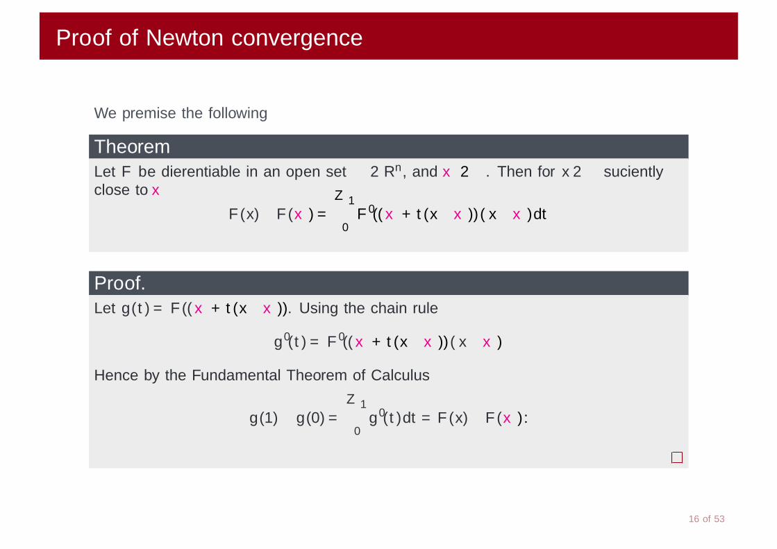
Proof of Newton convergence
We premise the following
TheoremLet F be differentiable in an open set Ω ∈ Rn, and x∗ ∈Ω. Then for x ∈Ω sufficientlyclose to x∗
F (x)−F (x∗) =∫ 1
0F ′((x∗+ t(x−x∗))(x−x∗)dt
Proof.Let g(t) = F ((x∗+ t(x−x∗)). Using the chain rule
g ′(t) = F ′((x∗+ t(x−x∗))(x−x∗)
Hence by the Fundamental Theorem of Calculus
g(1)−g(0) =∫ 1
0g ′(t)dt = F (x)−F (x∗).
16 of 53

Proof of Newton convergence
We now need two further results. The first one is also known as Banach Lemma
LemmaLet A,B square n×n matrices, and B such that ‖I −BA‖< 1. Then A,B are bothnonsingular and
‖A−1‖ ≤ ‖B‖1−‖I −BA‖
.
LemmaLet the standard assumptions hold. Then there is δ > 0 so that for allx ∈B(δ) = x : ‖x−x∗‖< δ the following hold true:
‖F ′(x)‖ ≤ 2‖F ′(x∗)‖ (7)
‖F ′(x)−1‖ ≤ 2‖F ′(x∗)−1‖ (8)
‖F(x)‖ ≤ 2‖F ′(x∗)‖‖e‖ (9)
17 of 53

Proof of Newton convergence
Proof.(7). By triangular inequality and Lipschitz continuity
‖F ′(x)‖−‖F ′(x∗)‖ ≤ ‖F ′(x)−F ′(x∗)‖ ≤ γ‖x−x∗‖= γ‖e‖ ≤ γδ .
Now if δ <‖F ′(x∗)‖
γthen ‖F ′(x)‖ ≤ ‖F ′(x∗)‖+ γδ ≤ 2‖F ′(x∗)‖ .
(8). Choosing now δ <1
2γ‖F ′(x∗)−1‖then
‖I −F ′(x∗)−1F ′(x)‖= ‖F ′(x∗)−1‖‖F ′(x∗)−F ′(x)‖ ≤ ‖F ′(x∗)−1‖γ‖e‖ ≤ 1
2.
Then applying Banach’s Lemma
‖F ′(x)−1‖ ≤ ‖F ′(x∗)−1
1−‖I −F ′(x∗)−1F ′(x)‖≤ ‖F
′(x∗)−1‖1−1/2
= 2‖F ′(x∗)−1‖.
(9). Using the previous Theorem and (8) yield
‖F(x)‖ ≤∫ 1
0‖F ′(x∗+ te)‖‖e‖dt ≤
∫ 1
02‖F ′(x∗)‖‖e‖dt = 2‖F ′(x∗)‖‖e‖.
18 of 53

Proof of Newton convergence
We are now able to prove the main theorem.
Proof.Let δ be smaller enough so that the previous Lemma holds.
ek+1 = xk+1−x∗ = xk −x∗−F ′(xk )−1F (xk )
= ek −F ′(xk )−1∫ 1
0F ′((x∗+ t(xk −x∗))ekdt
= F ′(xk )−1∫ 1
0
(F ′(xk )−F ′((x∗+ t(xk −x∗))
)ekdt.
Taking norms and again using Lipschitz continuity
‖ek+1‖ ≤ ‖F ′(xk )−1‖∫ 1
0γ‖xk −x∗− t(xk −x∗)‖‖ek‖dt
= ‖F ′(xk )−1‖γ‖ek‖2∫ 1
0(1− t)dt ≤ γ‖F ′(x∗)−1‖‖ek‖2 = K‖ek‖2.
19 of 53
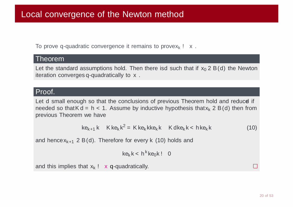
Local convergence of the Newton method
To prove q-quadratic convergence it remains to prove xk → x∗.
TheoremLet the standard assumptions hold. Then there is δ such that if x0 ∈ B(δ) the Newtoniteration converges q-quadratically to x∗.
Proof.Let δ small enough so that the conclusions of previous Theorem hold and reduce δ ifneeded so that Kδ = η < 1. Assume by inductive hypothesis that xk ∈ B(δ) then fromprevious Theorem we have
‖ek+1‖ ≤ K‖ek‖2 = K‖ek‖‖ek‖ ≤ Kδ‖ek‖< η‖ek‖ (10)
and hence xk+1 ∈ B(δ). Therefore for every k (10) holds and
‖ek‖< ηk‖e0‖→ 0
and this implies that xk → x∗q-quadratically.
20 of 53

Exit test
Ideal exit test ‖ek‖< ε (absolute error)
or ‖ek‖< ε‖e0‖ (relative error); where ε is a prescribed tolerance.
As however x∗ is not known
Exit test on the relative residual. Stop when
‖F(xk )‖‖F(x0)‖
< ε
Exit test on the difference. Stop when
‖s‖= ‖xk+1−xk‖< ε
21 of 53
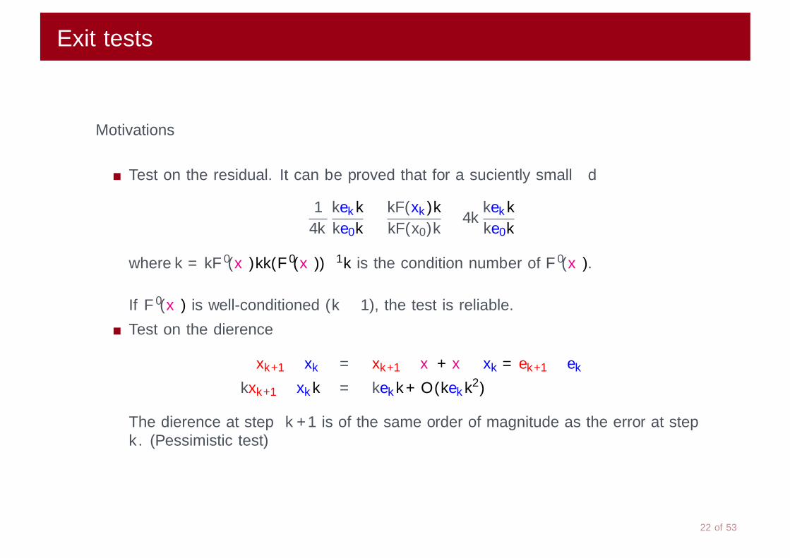
Exit tests
Motivations
Test on the residual. It can be proved that for a sufficiently small δ
1
4κ
‖ek‖‖e0‖
≤ ‖F(xk )‖‖F(x0)‖
≤ 4κ‖ek‖‖e0‖
where κ = ‖F ′(x∗)‖‖(F ′(x∗))−1‖ is the condition number of F ′(x∗).
If F ′(x∗) is well-conditioned (κ ≈ 1), the test is reliable.
Test on the difference
xk+1−xk = xk+1−x∗+ x∗−xk = ek+1−ek
‖xk+1−xk‖ = ‖ek‖+O(‖ek‖2)
The difference at step k + 1 is of the same order of magnitude as the error at stepk. (Pessimistic test)
22 of 53

Example
x2 +y2−4 = 0xy −1 = 0
x(0) =
(01
)
k x(k)1 x
(k)2 ‖e(k)‖ ‖x(k+1)−x(k)‖ ‖e(k+1)‖
‖e(k)‖2
0 0.000000000 1.000000000 0.107×10+01
1 1.000000000 2.500000000 0.745×10+00 0.180×10+01 0.6558992 0.595238095 2.011904761 0.111×10+00 0.634×10+00 0.2007163 0.520020336 1.934236023 0.337×10−02 0.108×10−00 0.2711534 0.517640404 1.931853966 0.327×10−05 0.337×10−02 0.2881145 0.517638090 1.931851652 0.309×10⁻¹¹ 0.327×10−05 0.288656
‖F(x(0))‖= 3.16 ‖F(x(1))‖= 3.58
23 of 53

Example
0 0.5 1 1.5 20.5
1
1.5
2
2.5
0 0.5 1 1.5 20.5
1
1.5
2
2.5
0 0.5 1 1.5 20.5
1
1.5
2
2.5
0 0.5 1 1.5 20.5
1
1.5
2
2.5
24 of 53

Global Convergence
Convergence of Newton’s method not guaranteed. Frequently Newton’s stepmoves away from the solution
To avoid divergence we accept Newton’s step if the following condition holds:‖F(xk+1)‖< ‖F(xk )‖ (simple decrease)
If the above condition is not satisfied, then the Newton step is reduced =⇒“backtracking” or “linesearch”.
Algorithm: Newton 2.
Given an initial approximation x0 , k := 0.
repeat until convergencesolve: F ′(xk )s =−F(xk )
• xt := xk + s
if ‖F (xt)‖< ‖F(xk )‖ then xk+1 := xt
else s := s/2, go to (• )
k := k + 1
25 of 53

Example: Newton with backtracking
x2 +y2−4 = 0xy −1 = 0
x(0) =
(01
)
k x(k)1 x
(k)2 ‖e(k)‖ x(k+1)−x(k) ‖e(k+1)‖
‖e(k)‖2
0 0.000000000 1.000000000 0.106597×10+01
1 0.500000000 1.750000000 0.182705×10+00 0.901388E+01 0.160790
‖F(x(0)))‖= 3.16 ‖F(x(1))‖= 0.699
0 0.5 1 1.5 20.5
1
1.5
2
2.5
26 of 53

Global Convergence: Armijo rule
With previous algorithm there is possibility of oscillation about the solution withoutconvergence.
To overcome this problem, the idea is to proceed in the Newton direction with
xk+1 = xk + αksk .
where αk is the largest value for which there is a sufficient decrease, namely
‖F(xk + αksk )‖< (1−ηαk )‖F(xk )‖.
η is usually a small parameter (η = 0 yields again algorithm: Newton 2)
27 of 53

Line search: polynomial interpolation
Suppose we have computed a scalar α which does not satisfy any decrease condition
Construct a 2nd degree interpolating polynomial p(x) using the function
g(t) = ‖F(xk + tsk )‖22
and the following (available) data
1 g(0)≡ ‖F(xk )‖22 ≡ p(0)
2 g ′(0) = 2(F ′(xk )sk )T F(xk ) = 2F(xk )TF ′(xk )sk =−2‖F(xk )‖2 ≡ p′(0).
3 g(α) = ‖F(xk + αsk )‖22 ≡ p(α)
The interpolating polynomial takes the following expression
p(x) = g(0) +g ′(0)x +g(α)−g(0)−g ′(0)α
α2x2 ≡ g(0) +g ′(0)x +cx2.
We are interested in the minimum of p(x),x ∈ [0,α].
Clearly g ′(0) < 0. Hence since g(α) > g(0) then c > 0 (convex parabola) and p(x) hasa minimum at
αk =−g ′(0)
2c> 0.
28 of 53

Inexact Newton Methods
Idea: Avoid Oversolving linear systems when too far from the nonlinear solution.
Recall the Newton iteration:
Solve: F ′(xk )s =−F(xk )
xk+1 := xk + s
k := k + 1
We want to solve the linear system by an iterative method with variable tolerance.
‖F ′(xk )s + F(xk )‖ ≤ ηk‖F(xk )‖
to control the accuracy of the linear system (sequence ηk).
ηk can be “large” at the beginning of Newton iteration since xk is likely far fromx∗,
ηk must be however sufficiently small towards the end of the Newton iteration.
Inexact Newton theory is aimed at properly choosing ηk to maintain Newtonconvergence properties.
29 of 53

Inexact Newton method. Theory
TheoremLet the standard assumptions hold. Then there are δ and K such that if xk ∈ B(δ)then s satisfies
‖F ′(xk )s + F(xk )‖ ≤ ηk‖F(xk )‖ (11)
and ‖ek+1‖ ≤ K (‖ek‖+ ηk )‖ek‖.
Proof.Let δ be small enough such that the conclusions of Newton convergece Theoremholds. Now defining r =−F ′(xk )s−F(xk ) (the residual of Newton’s system), then
s +F ′(xk )−1F(xk ) =−F ′(xk )−1r.
From (11) and recalling that ‖F ′(xk )−1‖ ≤ 2‖F ′(x∗)−1‖ and that‖F(xk )‖ ≤ 2‖F ′(x∗)‖‖ek‖,
‖s +F ′(xk )−1F(xk )‖ ≤ ‖F ′(xk )−1‖ηk‖F(xk )‖ ≤ 4κ(F ′(x∗))ηk‖ek‖.
Finally fromek+1 = ek −F ′(xk )−1F(xk ) + s +F ′(xk )−1F(xk )
taking norms we obtain
‖ek+1‖ ≤ K‖ek‖2 + 4κ(F ′(x∗))ηk‖ek‖= ‖ek‖
K︷ ︸︸ ︷(K + 4κ(F ′(x∗))
)(ηk +‖ek‖).

Main result
TheoremLet the standard assumptions hold. Then there are δ and η such that if x0 ∈ B(δ),ηk ∈⊂ [0, η], then
a) the inexact Newton iteration converges q-linearly to x∗. Moreover
b) If ηk → 0 then convergence is q-superlinear.
c) If ηk ≤ Kη‖F(xk )‖ for some Kη > 0 then the convergence is q-quadratic.
Proof.Let δ be the same as in the previous Theorem. Reduce it and η so that
K(δ + η) < 1.
a) Then if xk ∈ B(δ) q-linear convergence is proved since
‖ek+1‖ ≤ K (‖ek‖+ ηk )‖ek‖ ≤ K(δ + η)‖ek‖< ‖ek‖.
b) If ηk → 0 the q-superlinear convergence follows from the definition.
c) If ηk ≤ Kη‖F(xk )‖ using the previous theorem and (9) we write
‖ek+1‖ ≤ K (‖ek‖+Kη‖F(xk )‖)‖ek‖ ≤ K(‖ek‖+Kη 2‖F ′(x∗)‖‖ek‖
)‖ek‖
= K(1 +Kη 2‖F ′(x∗)‖
)︸ ︷︷ ︸K0
‖ek‖2 = K0‖ek‖2

Practical choices for ηk
The sequence ηk is usually set to
ηk =
ηmax if k = 0
γ‖F(xk )‖2
‖F(xk−1)‖2if k > 0
ηmax is chosen to be slightly less than 1
γ is a parameter in (0,1). This choice of ηk guarantees quadratic convergence,since ‖F(xk )‖= O(‖F(xk−1)‖2) =⇒ ηk = O(‖F(xk )‖).
S. C. Eisenstat and H. F. WalkerSIAM J. Sci. Comput., 17(1), 16–32. (17 pages)Choosing the Forcing Terms in an Inexact Newton Method
32 of 53

Quasi-Newton Methods
Motivation: Jacobian matrix
Not always explicitly available (sometimes function F is known as a set of data)
or
Differentiation of F may be too costly to be afforded at every Newton iteration
A possible answer to this problem is given by the quasi-Newton methods whichcompute a sequence of approximate Jacobians possibly starting from the ’true’ initialJacobian.
Instead of solvingxk+1 = xk −F′(xk )−1F(xk )
we solvexk+1 = xk −Bk
−1F(xk )
33 of 53
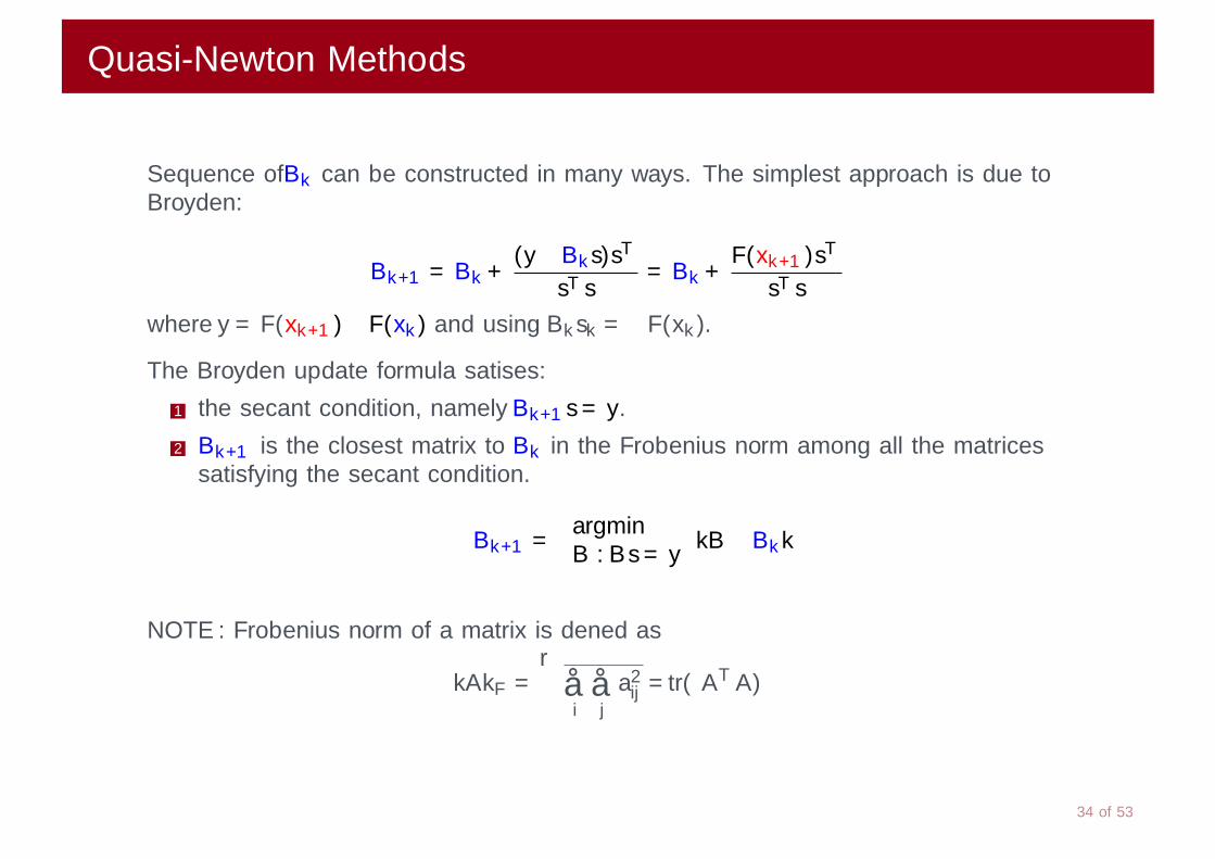
Quasi-Newton Methods
Sequence of Bk can be constructed in many ways. The simplest approach is due toBroyden:
Bk+1 = Bk +(y−Bks)sT
sT s= Bk +
F(xk+1)sT
sT s
where y = F(xk+1)−F(xk ) and using Bksk =−F(xk ).
The Broyden update formula satisfies:
1 the secant condition, namely Bk+1s = y.
2 Bk+1 is the closest matrix to Bk in the Frobenius norm among all the matricessatisfying the secant condition.
Bk+1 =argminB : Bs = y
‖B−Bk‖
NOTE: Frobenius norm of a matrix is defined as
‖A‖F =√
∑i
∑j
a2ij = tr(ATA)
34 of 53

Quasi-Newton Methods
The secant condition Bk+1s = y is a generalization of the secant method:
xk+1 = xk −f (xk )
bk
where
bk =f (xk )− f (xk−1)
xk −xk−1=
y
s.
In n dimension, the secant condition has an infinite number of solutions.
Broyden’s choice satisfies secant condition, in fact
Bk+1s = Bks +(y−Bks)sT
sT ss = Bks + y−Bks = y.
Broyden’s choice satisfies the least change condition.
‖Bk+1−Bk‖ =
∥∥∥∥ (y−Bks)sT
sT s
∥∥∥∥F
=
∥∥∥∥ (Bs−Bks)sT
sT s
∥∥∥∥F
=
=
∥∥∥∥ (B−Bk )ssT
sT s
∥∥∥∥F
≤ ‖B−Bk‖F∥∥∥∥ ssT
sT s
∥∥∥∥F
= ‖B−Bk‖F .
using∥∥∥ ssT
sT s
∥∥∥F
= 1 (proof by exercise).35 of 53

Convergence Results
DefinitionA sequence xk converges superlinearly to x∗ if there are α > 1 and K > 0 such that
‖xk+1−x∗‖ ≤ K‖xk −x∗‖α
Let us now define the error in jacobian approximations:
Ek = Bk −F ′(x∗)
The first Theorem states that the difference between the exact and the approximateJacobian does not grow with the Newton iteration. This property is also calledbounded deterioration.
Theorem
‖Ek+1‖ ≤ ‖Ek‖+γ
2(‖ek‖+‖ek+1‖)
36 of 53

Convergence Results and implementation
TheoremLet the standard assumption holds. Then there are δ and δB such that if ‖e0‖< δ and‖E0‖< δB the Broyden sequence exists and xk → x∗ superlinearly.
This theorem states that we can make ‖Ek‖ as small as we want by properly choosingthe initial vector x0 and the initial Jacobian approximation B0.
If it is the case, the convergence of the iteration remains very fast (superlinearconvergence).
Problem.How to implement solution of Newton system with Bk
−1 instead of J(xk )−1 ?Note that even if B0 is sparse B1 is not.
Careful implementation should avoid inversion of dense matrices.
37 of 53

Sparse implementation of Broyden method: Sherman Morrisonformula.
Theorem
(B + uvT )−1 =
(I − (B−1u)vT
1 + vTB−1u
)B−1 = B−1− (B−1u)vTB−1
1 + vTB−1u
Proof.Let us look for the inverse of B + uvT as B−1 + xyT . The following conditions must hold:
(1) I = (B + uvT ) · (B−1 + xyT ) = I + uvTB−1 +BxyT + uvT xyT
(2) I = (B−1 + xyT ) · (B + uvT ) = I + xyTB +B−1uvT + xyT uvT
Multiplying the first by u on the right and the second by vT on the left yields:
u(vTB−1u
)+Bx(yT u) + u(vT xyT u) = 0 =⇒ x = αB−1u.
(vT x)yTB + (vTB−1u)vT + (vT xyT u)vT = 0 =⇒ y = βB−1v.
Without loss of generality set β = 1 hence substituting in (1) we obtain
0 = uvTB−1 + αuvTB−1 + uvTαB−1uvTB−1 = uvTB−1
(1 + α(1 + vTB−1u)
)Finally we get α =
−1
1 + vTB−1uwhich completes the proof.
38 of 53
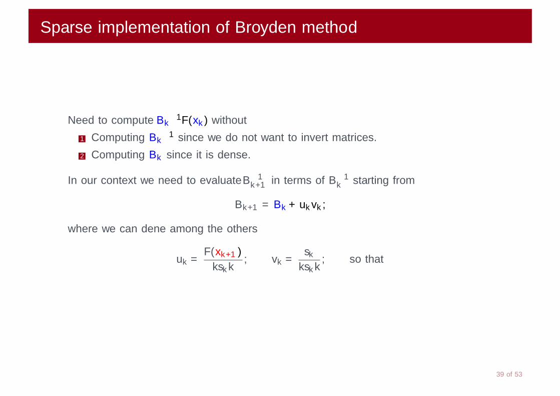
Sparse implementation of Broyden method
Need to compute Bk−1F(xk ) without
1 Computing Bk−1 since we do not want to invert matrices.
2 Computing Bk since it is dense.
In our context we need to evaluate B−1k+1 in terms of B−1
k starting from
Bk+1 = Bk + ukvk ,
where we can define among the others
uk =F(xk+1)
‖sk‖, vk =
sk‖sk‖
, so that
39 of 53
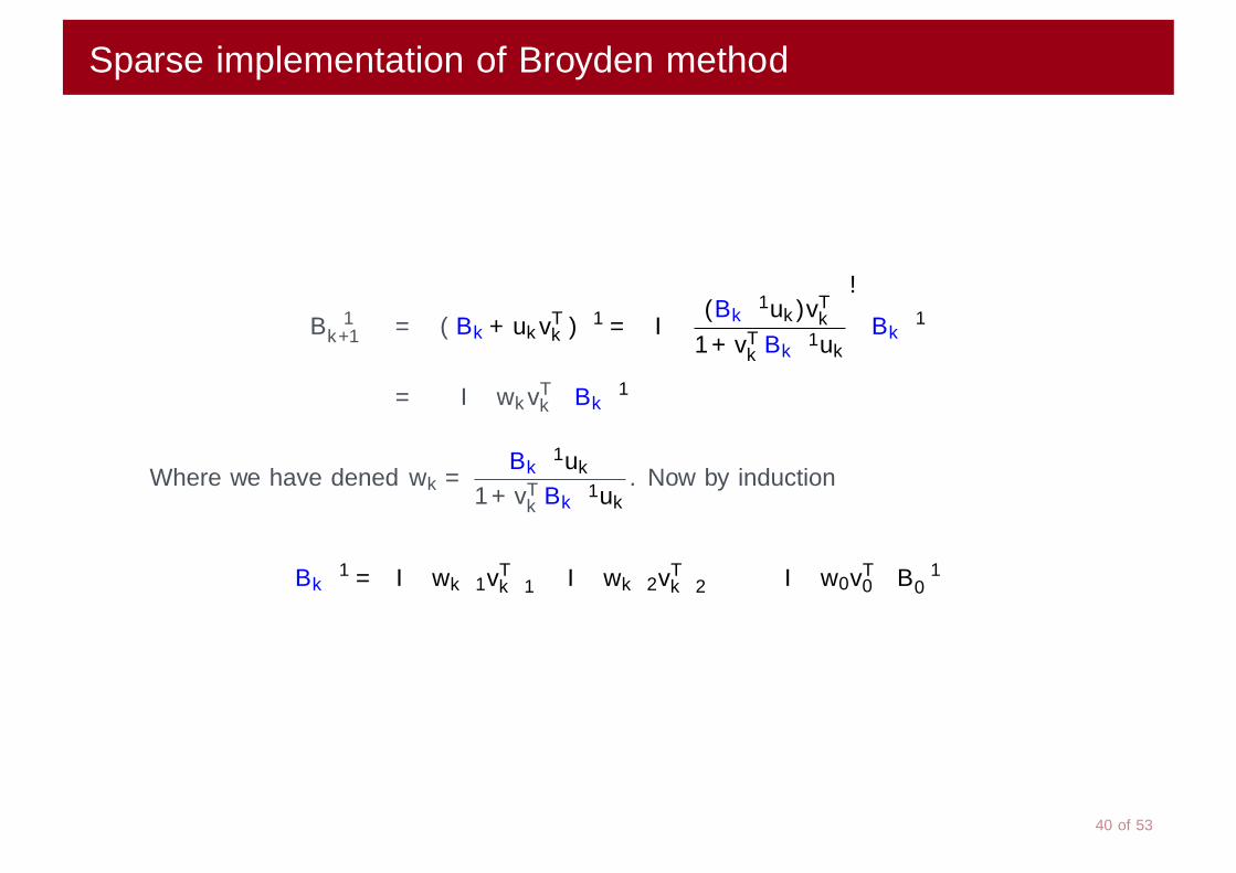
Sparse implementation of Broyden method
B−1k+1 = (Bk + ukvTk )−1 =
(I −
(Bk−1uk )vTk
1 + vTk Bk−1uk
)Bk−1
=(I −wkvTk
)Bk−1
Where we have defined wk =Bk−1uk
1 + vTk Bk−1uk
. Now by induction
Bk−1 =
(I −wk−1vTk−1
)(I −wk−2vTk−2
)· · ·(I −w0vT0
)B−1
0
40 of 53

Sparse implementation of Broyden method
Important results: sk =−Bk−1Fk is accomplished by
1 Solving the system B0z0 =−Fk
2 Computing α0 = wT0 z0, then z1 = z0−α0w0
Computing α1 = wT1 z1, then z2 = z1−α1w1
· · ·Computing αk−1 = wT
k−1zk−1, then zk = zk−1−αk−1wk−1
Problem. We do not know how to compute wj , j = 1, · · · ,k−1. Let us define
p = B−1k−1F(xk ) =
(I −wk−2vTk−2
)· · ·(I −w0vT0
)B−1
0 F(xk )
It follows that
sk = −Bk−1Fk =−
(I −wk−1vTk−1
)p = wk−1(vTk−1p)−p
B−1k−1uk−1 = B−1
k−1
Fk
‖sk−1‖=
p
‖sk−1‖
wk−1 =B−1k−1uk−1
1 + vTk−1B−1k−1uk−1
=p
‖sk−1‖+ vTk−1p
41 of 53
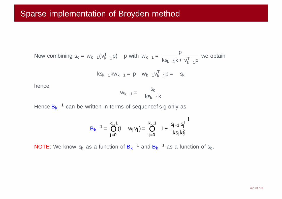
Sparse implementation of Broyden method
Now combining sk = wk−1(vTk−1p)−p with wk−1 =p
‖sk−1‖+ vTk−1pwe obtain
‖sk−1‖wk−1 = p−wk−1vTk−1p =−sk
hencewk−1 =− sk
‖sk−1‖
Hence Bk−1 can be written in terms of sequence sj only as
Bk−1 =
k−1
∏j=0
(I −wjvj ) =k−1
∏j=0
(I +
sj+1sTj‖sj‖2
2
)
NOTE: We know sk as a function of Bk−1 and Bk
−1 as a function of sk .
42 of 53

Sparse implementation of Broyden method
Let us write sk+1 as
sk+1 =−Bk+1−1Fk+1 = −
(I +
sk+1sTk‖sk‖2
2
)k−1
∏j=1
(I +
sj+1sTj‖sj‖2
2
)B−1
0 Fk
= −
(I +
sk+1sTk‖sk‖2
2
)Bk−1Fk+1
or
sk+1 =−B−1k Fk+1− sk+1
sTk B−1k Fk+1
‖sk‖22
Finally solve for sk+1 to obtain
sk+1 =−B−1
k Fk+1
1 + sTk B−1k Fk+1/‖sk‖2
2
43 of 53

Broyden Algorithm (sketch)
INPUT: x0,B0. Set k := 0,x := x0.
First step: Solve B0s0 =−F(x0)
repeat until convergence
x := x + sk
Solve B0z =−F(x)
k := k + 1.
for j := 0 to k−1
z := z + sj+1
sTj z
‖sj‖22
end for
sk+1 :=z
1− sTk z/‖sk‖22
end repeat
1 Only a system with B0 needed to be solved at each Newton step.
2 k scalar products and 1 vector norm at k-th step. Complexity increasing with k.
44 of 53

Exercise
The nonlinear Bratu problem is defined as
Au + λ exp(u)u = 0
where exp(u)≡(exp(u1), . . . ,exp(un)
)T, A is the Finite Difference discretization of the
Laplacian in the unit square, λ ∈ [0,6.8] is a real parameter.
ExerciseWrite a Matlab script which computes the (scaled) FD discretization of the Laplacianin the unit square (Recall that the delsq function returns −A) with h = 0.01, sets λ = 6.5×h2
and solves the Bratu problem using a constant x0 with all components equal to = 0.1and stopping when the relative residual is smaller than 10−6, with the followingalgorithms:
1 Newton’s method with the solution of the linear systems by a direct method.
2 Broyden method with the solution of the linear systems by a direct method.
3 Inexact Newton method with the solution of the linear systems using the GMRESmethod with p = 30 (restart parameter) and three sequences of tolerance ηk :
1 ηk = 10−2, ∀k2 η0 = 10−2, ηk+1 =
ηk2 , k ≥ 0
3 ηk = min10−2,‖F(xk )‖
45 of 53

Exercise: continued
ExerciseThe script must also
Display the results as a table in which every row represents a single Newtoniteration showing the iteration number, the residual norm, and, in case ofiterative solution of the Newton system, also the tolerance and the number ofGMRES iterations.
Produce two figures with the semilogarithmic convergence profile (residual normvs number of nonlinear iteration) of the methods. The first picture should plotthe Newton vs Quasi-Newton profiles. The second one the Newton profile (withdirect method) vs Inexact Newton profiles with the three choices of ηk .
46 of 53

Bibliography
C. T. Kelley
Iterative methods for optimization,
SIAM, Frontiers in Applied Mathematics, 1999
R. S. Dembo and S C. Eisenstat and T. Steihaug,
Inexact Newton Methods,
SIAM Journal on Numerical Analysis, 1982
J. E. Dennis and J. J. More,
Quasi-Newton methods, motivation and theory,
SIAM Reviews, 1977
47 of 53

Function minimization
Consider a function f : Rn→ R.
Our aim is to solve the problem
minx
f (x). (Unconstrained minimization)
i.e. to find the vector x∗ such that
f (x∗)≤ f (x), ∀x ∈ Rn.
Suppose f is continuously differentiable and convex. Then it can be proved that alocal minimizer is also a global minimizer.
Every method therefore tries to approximate the solution of
∇f (x) = 0.
with an iteration of the form
xk+1 = xk + αkp.
48 of 53

Direction of decrease
Suppose f twice differentiable and H(x) its Hessian, then
f (xk + αp) = f (xk ) + α∇f (xk )T p +1
2α
2pTH(xk + tp)p, t ∈ (0,α).
Taking α > 0, the direction p is defined a descent direction if
∇f (xk )T p < 0.
Considering only the first order term in the Taylor expansion, the direction of mostrapid decrease is pk =−∇f (xk ).
With this choice we have the method of the steepest descent.
The method may be very slow (recall the SD for linear systems)
There is no way to compute the optimal value of α.
49 of 53

Newton’s method
There is an important alternative to the (minus) gradient direction.
Let us consider now the second order approximation for the function
f (xk + αp)≈ f (xk ) + α∇f (xk )T p +1
2α
2pTH(xk )p≡mk (p)
By simply settin the derivative of mk (p) to zero we obtain the Newton direction
pNk = H(xk )−1
∇f (xk ),
which is a reliable direction if the difference between the function and the model is nottoo large (note that f (xk + αp)−mk (p) = O(‖p‖3).)
TheoremIf f is convex than the Newton direction is a direction of decrease for f .
Proof.Since f is convex, then the Hessian is symmetric positive definite, hence
∇f Tk pNk =−pN
k H(xk )pNk =−σk‖pN
k ‖2,
for some σ > 0.
50 of 53

Computing the step length
Defineφ(α) = f (xk + αp), α > 0.
Our goal is to find the minimum of φ(α). However, solving exactly φ ′(α) = 0 is not realistic.
First we define a condition under which we accept the step αp.
Definition (Wolfe conditions)
The Wolfe conditions for accepting a step αpk are:
f (xk + αpk ) ≤ f (xk ) +c1α∇fkpk sufficient decrease condition (12)
∇f (xk + αpk )T pk ≥ c2∇f (xk )T pk curvature condition (13)
(12): the reduction in f should be proportional to both α and the directional derivative ∇f Tk pk .
(13): the reduction rate of f in xk + αpk is greater than that of f in xk (times a constant c2).
A strongly negative reduction rate predicts that we can reduce further f along this direction andwe do not accept α.
Algorithm:linesearch + backtracking
1: Choose ρ < 1.2: α = 13: while Wolf conditions not verified do4: α = ρα
5: end while

Trust region methods
First consider an approximate (quadratic model) of the function f
mk (p) = f (xk ) + pT∇fk +
1
2pTBp,
where B is either the Hessian of f or some (QuasiNewton) approximation of it.
Then we try to find the minimum of mk (p).
However, to guarantee that mk (p) and f (xk + p) are sufficiently close, we restrict thesearch for a minimizer of mk to some region close to xk .
Usually this region is‖p‖2 ≤∆,
with ∆ > 0 the radius of the trust region.
In summary the following constrained minimization problem is to be solved at eachstep:
minp
f (xk ) + pT∇fk +
1
2pTBp such that ‖p‖2 ≤∆k
52 of 53

Trust region: implementation
Question: How to choose the trust region radius?
Define
ρ =f (xk )− f (xk + p)
mk (0)−mk (p)=
actual reduction
expected reduction
Notice than the denominator is positive since p is the minimizer.
if ρ
is negative or close to zero reduce ∆
is significantly < 1 leave ∆ unchanged
is close to 1 increase ∆
To compute the miminizer, recall this important results
TheoremThe vector p∗ is the global minimizer of the constrained problem if and only if p∗ isfeasible (satisfies the constraint) and there exists λ ≥ 0 such that
(B + λ I )p∗ = −∇f (xk )
λ (∆−‖p∗‖2) = 0
B + λ I is positive semidefinite