Embed Size (px)
Citation preview

NEWTON Deliverable D3.1
Preliminary design report for the magnetic head
Project Number: 730041
Project Title New portable multi-sensor scientific instrument for non-invasive on-site characterisation of rock from planetary surface and sub-surfaces.
Deliverable Type: Public
Title: Deliverable D3.1 - Preliminary design report for the
magnetic headWork Package: Work Package 3Responsible: INTA Due Date: 31.10.2017Nature: ReportSecurity: PublicVersion: 1.0Authors: TTI: Laura González , Cristina Lavín, Adrián Sánchez INTA: Javier de Frutos, Marina Díaz Michelena, José Luis Mesa, Miguel Ángel Rivero UPM: Claudio Aroca, Pedro Cobos , Marco Maicas, Marina Pérez , Mar Sanz UT: Rolf Kilian
Abstract: NEWTON multi-sensor instrument (prototypes 1-3) is integrated by three different key building blocks which are the Power Distribution Unit (PDU), the electronic Control Unit (CU) and the Sensor Unit (SU). The magnetic head is allocated in the SU. This sensor unit contains the susceptometer head and the magnetometer as well as two electronic PCBs for the proximity electronic (reading and exciting).This document reports the preliminary design and optimization process of the magnetic head, including susceptometer head and magnetometer.
Keyword list: Planetary Science, magnetometry, complex susceptibility, multi-sensor system, Mars, the Moon, control unit, lock-in, signal processing, susceptometer, magnetometer, magnetic amplifier.
Disclaimer: This document reflects the contribution of the participants of the research project NEWTON. The European Union and its agencies are not liable or otherwise responsible for the contents of this document; its content reflects the view of its authors only. This document is provided without any warranty and does not constitute any commitment by any participant as to its content, and specifically excludes any warranty of correctness or fitness for a particular purpose. The user will use this document at the user's sole risk.
D3.1 - Preliminary design report for the magnetic head
NEWTON Grant agreement no: 730041 Page 2 of 53 31 Oct. 17
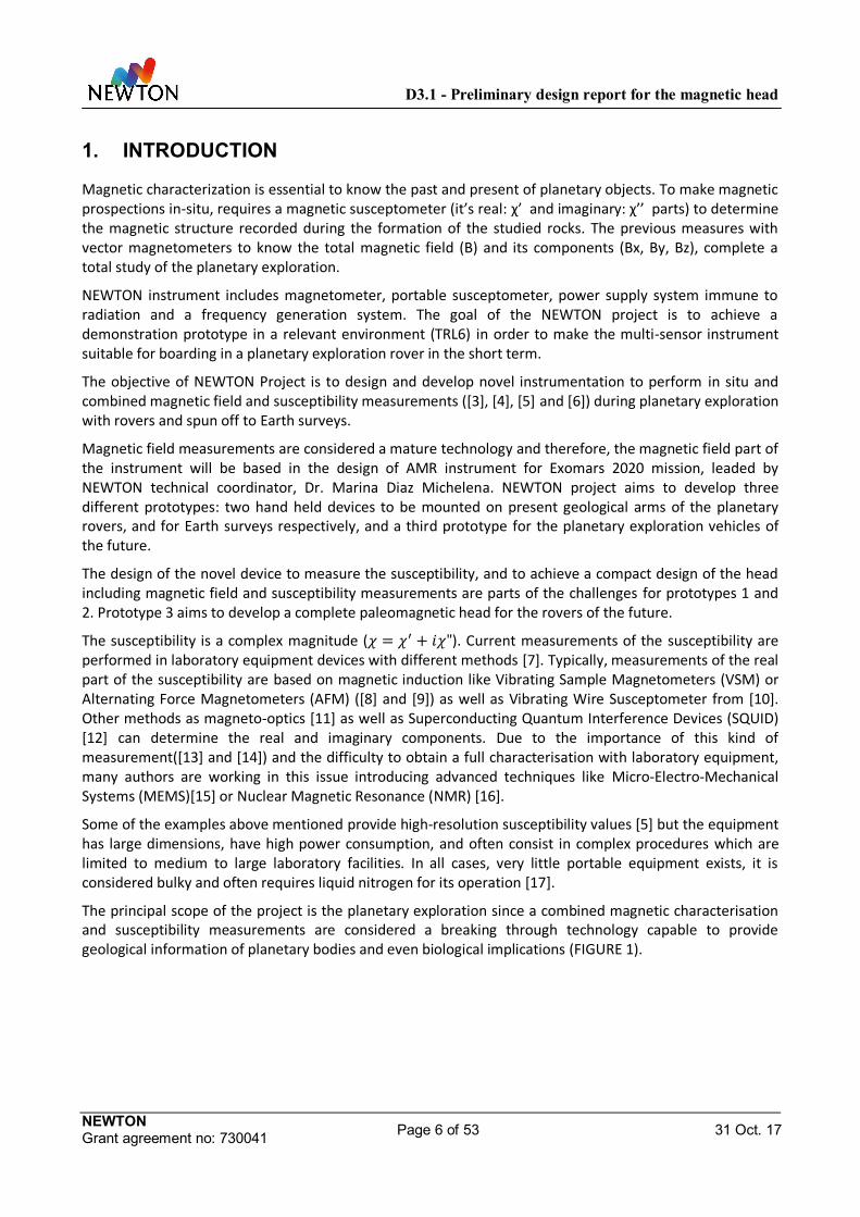
Executive Summary This NEWTON WP3 deliverable D3.1 entitled "Preliminary design report for the magnetic head" describes the preliminary design of the magnetic head (included in the Sensor Unit), developed for the three prototypes of NEWTON instrument.
With the aim of maximizing the impact of novel NEWTON technology, different prototypes will be developed within the project. Two prototypes (named prototype 1 and 3) will be developed for planetary application, while a slightly (reduced) adapted version of prototype 1 (named prototype 2) will be developed in order to demonstrate the spin-off of the technology between space and non-space fields. The three prototypes share the same architecture while they provide different performance capabilities adapted to different scenarios. The key building blocks of the three prototypes are the same, i.e. Power Distribution Unit (PDU), the electronic Control Unit (CU) and the Sensor Unit (SU).
The magnetic head is allocated in the SU. This sensor unit contains the susceptometer head and the magnetometer as well as two electronic PCBs for the proximity electronic (reading and exciting).This document (D3.1) reports the preliminary design and optimization process of the magnetic head including susceptometer head and magnetometer, which complies successfully the objectives stated in the proposal. The preliminary design of the electronics for the SU is included in D3.2 [1] which also reports the preliminary design of the Control Unit. Additionally, D3.3 [2] reports the preliminary design of the Power Distribution Unit and part of the excitation system.
This document is structured in different sections. Section 2 reports the architecture of the three prototypes developed within the NEWTON project as well as it describes the main differences between them. Section 3 describes the preliminary design of the magnetic head for the three prototypes of the NEWTON instrument including innovations in the design and main difficulties solved along the design process. Section 4 reports the main results obtained from the preliminary validation tests as a preliminary proof of the consecution of the objectives. Finally, Section 5 presents a summary of the content included in this document, the main conclusions on the degree of advance obtained from it as well as the future lines of work and collaboration with other EU teams, and Section 6 provides the referenced bibliography.

D3.1 - Preliminary design report for the magnetic head
NEWTON Grant agreement no: 730041 Page 3 of 53 31 Oct. 17
Authors
Partner Name Email
TTI
Laura González [email protected]
Cristina Lavín [email protected]
Adrián Sánchez [email protected]
INTA
Javier de Frutos [email protected]
Marina Díaz-Michelena [email protected]
José Luis Mesa [email protected]
Miguel Ángel Rivero [email protected]
UPM
Claudio Aroca [email protected]
Pedro Cobos [email protected]
Marco Maicas [email protected]
Mar Sanz [email protected]
Marina Pérez [email protected]
Mar Sanz [email protected]
UT Rolf Kilian [email protected]

D3.1 - Preliminary design report for the magnetic head
NEWTON Grant agreement no: 730041 Page 4 of 53 31 Oct. 17
Table of Contents 1. INTRODUCTION ................................................................................................................. 6
2. ARCHITECTURE OF THE NEWTON INSTRUMENT .................................................... 8
2.1. NEWTON PROTOTYPE 1 AND PROTOTYPE 2 ............................................................... 8 2.2. NEWTON PROTOTYPE 3 ...................................................................................................11 2.3. COMPARISON OF NEWTON PROTOTYPES .................................................................13
3. PRELIMINARY DESIGN AND OPTIMIZATION OF THE MAGNETIC HEAD ........... 15
3.1. PROTOTYPE 1 AND 2 ....................................................................................................15 3.1.1. General operational requirements ................................................................................15 3.1.2. General design requirements ........................................................................................16 3.1.3. Working principle ............................................................................................................16 3.1.4. Design of the Magnetic Head .........................................................................................23 3.1.5. Optimization of the Electric Circuit ..............................................................................27 3.1.6. Optimization of the Magnetic Head ..............................................................................35 3.1.7. Requirements for the proximity electronics. ..............................................................39
3.2. PROTOTYPE 3 .....................................................................................................................40 3.2.1. Requirements ...................................................................................................................40 3.2.2. Magnetic measuring set-up ...........................................................................................42
4. RESULTS AND VALIDATION DATA ............................................................................. 47
4.1. VALIDATION DATA FOR PROTOTYPES 1 AND 2 ........................................................47 4.2. MANUFACTURING AND VALIDATION DATA FOR PROTOTYPE 3 ...........................48
5. SUMMARY AND CONCLUSIONS.................................................................................. 51
6. REFERENCES .................................................................................................................. 52

D3.1 - Preliminary design report for the magnetic head
NEWTON Grant agreement no: 730041 Page 5 of 53 31 Oct. 17
Abbreviations AC Alternating Current ADC Analog to Digital Converter AFM Alternating Force Magnetometers AMR Anisotropic Magneto Resistance B Magnetic Induction COTS Commercial off the shelf CU Control Unit D Deliverable DAC Digital to Analog Converter DC Direct Current DSP Digital Signal Processor EU European Union FS Fixed Susceptomter IEEE Institute of Electrical and Electronics Engineers INTA Instituto Nacional Técnica Aeroespacial “Esteban Terradas” IRM Isothermal Remanent Magnetization M Magnetization MEMS Micro Electro Mechanical System n Number of turns when N is used for demagnetizing factor N Number of turns / Demagnetizing factor NRM Natural Remanent Magnetization PC Personal Computer PCB Printed Circuit Board PDU Power Distribution Unit PS Portable Susceptomter R Resistance SH Sensor Head SQUID Superconducting Quantum Interference Devices SU Sensor Unit TBC To Be Completed TBD To Be Determined TRL Technology Readiness Level TTI Tecnologías de Telecomunicaciones e Información UPM Universidad Politécnica Madrid UT University of Trier VSM Vibrating Sample Magnetometers WP Work Package
D3.1 - Preliminary design report for the magnetic head
NEWTON Grant agreement no: 730041 Page 6 of 53 31 Oct. 17
1. INTRODUCTION
Magnetic characterization is essential to know the past and present of planetary objects. To make magnetic prospections in-situ, requires a magnetic susceptometer (it’s real: χ’ and imaginary: χ’’ parts) to determine the magnetic structure recorded during the formation of the studied rocks. The previous measures with vector magnetometers to know the total magnetic field (B) and its components (Bx, By, Bz), complete a total study of the planetary exploration.
NEWTON instrument includes magnetometer, portable susceptometer, power supply system immune to radiation and a frequency generation system. The goal of the NEWTON project is to achieve a demonstration prototype in a relevant environment (TRL6) in order to make the multi-sensor instrument suitable for boarding in a planetary exploration rover in the short term.
The objective of NEWTON Project is to design and develop novel instrumentation to perform in situ and combined magnetic field and susceptibility measurements ([3], [4], [5] and [6]) during planetary exploration with rovers and spun off to Earth surveys.
Magnetic field measurements are considered a mature technology and therefore, the magnetic field part of the instrument will be based in the design of AMR instrument for Exomars 2020 mission, leaded by NEWTON technical coordinator, Dr. Marina Diaz Michelena. NEWTON project aims to develop three different prototypes: two hand held devices to be mounted on present geological arms of the planetary rovers, and for Earth surveys respectively, and a third prototype for the planetary exploration vehicles of the future.
The design of the novel device to measure the susceptibility, and to achieve a compact design of the head including magnetic field and susceptibility measurements are parts of the challenges for prototypes 1 and 2. Prototype 3 aims to develop a complete paleomagnetic head for the rovers of the future.
The susceptibility is a complex magnitude ( = + "). Current measurements of the susceptibility are performed in laboratory equipment devices with different methods [7]. Typically, measurements of the real part of the susceptibility are based on magnetic induction like Vibrating Sample Magnetometers (VSM) or Alternating Force Magnetometers (AFM) ([8] and [9]) as well as Vibrating Wire Susceptometer from [10]. Other methods as magneto-optics [11] as well as Superconducting Quantum Interference Devices (SQUID) [12] can determine the real and imaginary components. Due to the importance of this kind of measurement([13] and [14]) and the difficulty to obtain a full characterisation with laboratory equipment, many authors are working in this issue introducing advanced techniques like Micro-Electro-Mechanical Systems (MEMS)[15] or Nuclear Magnetic Resonance (NMR) [16].
Some of the examples above mentioned provide high-resolution susceptibility values [5] but the equipment has large dimensions, have high power consumption, and often consist in complex procedures which are limited to medium to large laboratory facilities. In all cases, very little portable equipment exists, it is considered bulky and often requires liquid nitrogen for its operation [17].
The principal scope of the project is the planetary exploration since a combined magnetic characterisation and susceptibility measurements are considered a breaking through technology capable to provide geological information of planetary bodies and even biological implications (FIGURE 1).

D3.1 - Preliminary design report for the magnetic head
NEWTON Grant agreement no: 730041 Page 7 of 53 31 Oct. 17
FIGURE 1. Magnetic susceptibilities and X-ray fluorescence (Fe content & Fe/Ti ratios) of sediments from a
Patagonian lake (unpublished data of R. Kilian, reproduced in the proposal as fig. 1.8).
D3.1 - Preliminary design report for the magnetic head
NEWTON Grant agreement no: 730041 Page 8 of 53 31 Oct. 17
2. ARCHITECTURE OF THE NEWTON INSTRUMENT
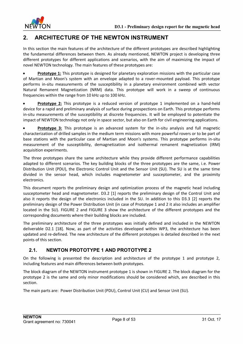
In this section the main features of the architecture of the different prototypes are described highlighting the fundamental differences between them. As already mentioned, NEWTON project is developing three different prototypes for different applications and scenarios, with the aim of maximizing the impact of novel NEWTON technology. The main features of these prototypes are:
Prototype 1: This prototype is designed for planetary exploration missions with the particular case of Martian and Moon's system with an envelope adapted to a rover-mounted payload. This prototype performs in-situ measurements of the susceptibility in a planetary environment combined with vector Natural Remanent Magnetization (NRM) data. This prototype will work in a sweep of continuous frequencies within the range from 10 kHz up to 100 kHz.
Prototype 2: This prototype is a reduced version of prototype 1 implemented on a hand-held device for a rapid and preliminary analysis of surface during prospections on Earth. This prototype performs in-situ measurements of the susceptibility at discrete frequencies. It will be employed to potentiate the impact of NEWTON technology not only in space sector, but also on Earth for civil engineering applications.
Prototype 3: This prototype is an advanced system for the in-situ analysis and full magnetic characterization of drilled samples in the medium term missions with more powerful rovers or to be part of base stations with the particular case of Martian and Moon's systems. This prototype performs in-situ measurement of the susceptibility, demagnetization and isothermal remanent magnetization (IRM) acquisition experiments.
The three prototypes share the same architecture while they provide different performance capabilities adapted to different scenarios. The key building blocks of the three prototypes are the same, i.e. Power Distribution Unit (PDU), the Electronic Control Unit and the Sensor Unit (SU). The SU is at the same time divided in the sensor head, which includes magnetometer and susceptometer, and the proximity electronics.
This document reports the preliminary design and optimization process of the magnetic head including susceptometer head and magnetometer. D3.2 [1] reports the preliminary design of the Control Unit and also it reports the design of the electronics included in the SU. In addition to this D3.3 [2] reports the preliminary design of the Power Distribution Unit (in case of Prototype 1 and 2 it also includes an amplifier located in the SU). FIGURE 2 and FIGURE 3 show the architecture of the different prototypes and the corresponding documents where their building blocks are included.
The preliminary architecture of the three prototypes was initially defined and included in the NEWTON deliverable D2.1 [18]. Now, as part of the activities developed within WP3, the architecture has been updated and re-defined. The new architecture of the different prototypes is detailed described in the next points of this section.
2.1. NEWTON PROTOTYPE 1 AND PROTOTYPE 2 On the following is presented the description and architecture of the prototype 1 and prototype 2, including features and main differences between both prototypes.
The block diagram of the NEWTON instrument prototype 1 is shown in FIGURE 2. The block diagram for the prototype 2 is the same and only minor modifications should be considered which, are described in this section.
The main parts are: Power Distribution Unit (PDU), Control Unit (CU) and Sensor Unit (SU).

D3.1 - Preliminary design report for the magnetic head
NEWTON Grant agreement no: 730041 Page 9 of 53 31 Oct. 17
FIGURE 2. Block Diagram of the NEWTON muti-sensor instrument for prototype 1 and prototype 2.
The Power Distribution Unit
The Power Distribution Unit supplies energy to the Control and to the Sensor Unit.
The PDU is integrated by the power module, i.e. DC/DC converter and the AC current source. In the case of prototype 1 and 2, it is not required to design an independent AC current source so it will be implemented as part of the Control Unit and Sensor Unit. It includes a power inverter to change direct current into alternating current (DC/AC). The alternating voltage working cycle is controlled by a microprocessor and continuous voltage is controlled by magnetic transformers.
On one hand, the DC/DC converter receives the primary power from the rover or external batteries, i.e. 28 V not regulated, and generates the secondary lines to supply the Sensor and the Control Units. The requirements of the DC/DC converter are the same for prototype 1 and prototype 2. On the other hand, the AC current source and impedance matching module generate the current to drive the primary winding of the sensor unit.
The Control Unit
The Electronic Control Unit is the responsible of the control, acquisition and processing of the signals of the sensor unit. The microcontroller performs these tasks as well as generates the different frequency signals for the susceptometer and magnetometer. The detection will have scalable performance between the different prototypes. Apart from the micro controller, the CU includes an oscillator to generate a stable reference frequency and a memory to save the input data measurements. The lock-in amplifier is allocated
D3.1
D3.2
D3.3
D3.3

D3.1 - Preliminary design report for the magnetic head
NEWTON Grant agreement no: 730041 Page 10 of 53 31 Oct. 17
inside the SU module to be able to perform an analog lock in. A Digital Signal Processing (DSP) lock in was studied but it was discarded given the complexity involved in the sample rate required for the measuring frequency range (DC to 100 kHz).
The Sensor Unit.
The SU includes a Susceptometer and a Vector Magnetometer. As already mentioned in the introduction, NEWTON prototype 1 is being designed for planetary exploration missions, with the particular case of Mars and the Moon. The Vector Magnetometer measures the environmental magnetic field superimposed to the natural remanence of surface rocks, and the Susceptometer measures the magnetic complex susceptibility in a sweep of 40 to 50 kHz within the range of 10 to 100 kHz, and its envelope is adapted to a rover-mounted payload. NEWTON prototype 2, is a reduced version of prototype 1 implemented on a hand-held device for a rapid and preliminary analysis of surface during prospections on Earth. This instrument is capable of performing in-situ measurements of the local magnetic field and complex susceptibility.
The susceptometer is a novel induction based device, consisting of a ferrite core with H shape connected to a modified tank resonant circuit, with the capability to determine the complex magnetic susceptibility at different frequencies.
The H shaped ferrite core of the susceptometer allows to perform a differential measurement, which increases the sensitivity to measure the imaginary part of the susceptibility, very low in most of the rocks. The susceptometer ferrite core is constructed with a primary winding for the excitation and a couple of secondary coils in opposition for the measurements.
The Prototype 2 is similar to prototype 1, with the main difference that prototype 1 will include magnetic amplifiers for a continuous frequency sweep and prototype 2 will be tuned at a single frequency, as a simplified version for earth magnetic surveys.
Two different techniques for the characterization of the magnetic susceptibility are foreseen for prototypes 1 and 2. These two techniques will be described in detail in section 3. Both of them will use the lock in amplifier designed, which operates in dual-phase demodulation and can compute the phase shift.
With regard to the magnetometer, it is based on COTS AMR technology, a designed based on AMR instrument on board Exomars 2020.
As it will be seen, in order to find the best configuration to work at different frequencies, it will be considered the inclusion of magnetic amplifiers in the design of the susceptometer head.
Interface
The instrument has two electrical interfaces with the platform: communications (commands and data transfer) and power supply. The communication interface will be emulated by a PC (in prototypes 1 and 2) and the power interface will be implemented by means of a batteries set or a commercial power source. Prototype 1 and prototype 2 will be tested in field campaigns on different scientific demonstration sites selected for the project so external portable batteries are required to supply the instruments during the field verification and surveys.
More information on the differences between prototypes 1 and 2, and also the comparison with prototype 3 main features are presented in section 2.3.
D3.1 - Preliminary design report for the magnetic head
NEWTON Grant agreement no: 730041 Page 11 of 53 31 Oct. 17
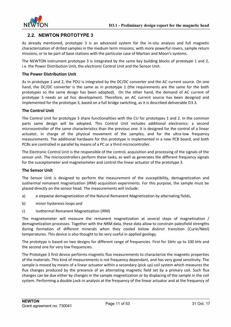
2.2. NEWTON PROTOTYPE 3 As already mentioned, prototype 3 is an advanced system for the in-situ analysis and full magnetic characterization of drilled samples in the medium term missions, with more powerful rovers, sample return missions, or to be part of base stations with the particular case of Martian and Moon's systems.
The NEWTON instrument prototype 3 is integrated by the same key building blocks of prototype 1 and 2, i.e. the Power Distribution Unit, the electronic Control Unit and the Sensor Unit.
The Power Distribution Unit
As in prototype 1 and 2, the PDU is integrated by the DC/DC converter and the AC current source. On one hand, the DC/DC converter is the same as in prototype 1 (the requirements are the same for the both prototypes so the same design has been adopted). On the other hand, the demand of AC current of prototype 3 needs an ad hoc development. Therefore, an AC current source has been designed and implemented for the prototype 3, based on a full bridge switching, as it is described deliverable D3.3.
The Control Unit
The Control Unit for prototype 3 share functionalities with the CU for prototypes 1 and 2. In the common parts same design will be adopted. This Control Unit includes additional electronics: a second microcontroller of the same characteristics than the previous one. It is designed for the control of a linear actuator, in charge of the physical movement of the samples, and for the ultra-low frequency measurements. The additional hardware for this prototype is implemented in a new PCB board, and both PCBs are controlled in parallel by means of a PC or a third microcontroller.
The Electronic Control Unit is the responsible of the control, acquisition and processing of the signals of the sensor unit. The microcontrollers perform these tasks, as well as generates the different frequency signals for the susceptometer and magnetometer and control the linear actuator of the prototype 3.
The Sensor Unit
The Sensor Unit is designed to perform the measurement of the susceptibility, demagnetization and isothermal remanent magnetization (IRM) acquisition experiments. For this purpose, the sample must be placed directly on the sensor head. The measurements will include:
a) a stepwise demagnetization of the Natural Remanent Magnetization by alternating fields,
b) minor hysteresis loops and
c) Isothermal Remanent Magnetization (IRM)
The magnetometer will measure the remanent magnetization at several steps of magnetization / demagnetization processes. Together with the NRM data, these data allow to constrain paleofield strengths during formation of different minerals when they cooled below distinct transition (Curie/Néel) temperatures. This device is also thought to be very useful in applied geology.
The prototype is based on two designs for different range of frequencies. First for 1kHz up to 100 kHz and the second one for very low frequencies.
The Prototype 3 first device performs magnetic flux measurements to characterize the magnetic properties of the materials. This kind of measurements is not frequency dependant, and has very good sensitivity. The sample is moved by means of a linear actuator within a secondary (pick up) coil system which measures the flux changes produced by the presence of an alternating magnetic field set by a primary coil. Such flux changes can be due either by changes in the sample magnetization or by displacing of the sample in the coil system. Performing a double Lock-in analysis at the frequency of the linear actuator and at the frequency of
D3.1 - Preliminary design report for the magnetic head
NEWTON Grant agreement no: 730041 Page 12 of 53 31 Oct. 17
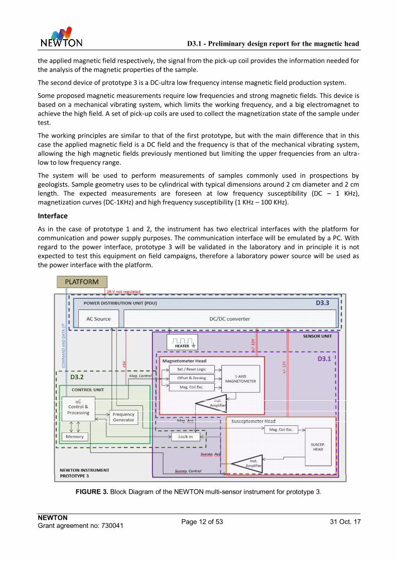
the applied magnetic field respectively, the signal from the pick-up coil provides the information needed for the analysis of the magnetic properties of the sample.
The second device of prototype 3 is a DC-ultra low frequency intense magnetic field production system.
Some proposed magnetic measurements require low frequencies and strong magnetic fields. This device is based on a mechanical vibrating system, which limits the working frequency, and a big electromagnet to achieve the high field. A set of pick-up coils are used to collect the magnetization state of the sample under test.
The working principles are similar to that of the first prototype, but with the main difference that in this case the applied magnetic field is a DC field and the frequency is that of the mechanical vibrating system, allowing the high magnetic fields previously mentioned but limiting the upper frequencies from an ultra-low to low frequency range.
The system will be used to perform measurements of samples commonly used in prospections by geologists. Sample geometry uses to be cylindrical with typical dimensions around 2 cm diameter and 2 cm length. The expected measurements are foreseen at low frequency susceptibility (DC – 1 KHz), magnetization curves (DC-1KHz) and high frequency susceptibility (1 KHz – 100 KHz).
Interface
As in the case of prototype 1 and 2, the instrument has two electrical interfaces with the platform for communication and power supply purposes. The communication interface will be emulated by a PC. With regard to the power interface, prototype 3 will be validated in the laboratory and in principle it is not expected to test this equipment on field campaigns, therefore a laboratory power source will be used as the power interface with the platform.
FIGURE 3. Block Diagram of the NEWTON multi-sensor instrument for prototype 3.
D3.3
D3.2
D3.1

D3.1 - Preliminary design report for the magnetic head
NEWTON Grant agreement no: 730041 Page 13 of 53 31 Oct. 17
As it can be seen from the block diagrams for the different prototypes (FIGURE 2 and FIGURE 3), the different units are well differenced and they would be placed in different physical parts of the platform. Regarding this location, the different units have different exposure levels to hard conditions environments, i.e. temperature, vibration or radiation. In the case of prototype 2, as it is devoted to earth field measurements, the qualification level of its components is that for common commercial instruments. In the case of prototype 1 and 3, designed for space applications, we must distinguish between the units and its potential location. While the CU and the PDU of both prototypes, and the SU of prototype 3 are to be placed within the inner of the rover body, which provides a relative protection against the severe planetary conditions, the SU of prototype 1 will be exposed to such conditions, what implies a more specific qualification of the different parts considered in the construction of this device.
2.3. COMPARISON OF NEWTON PROTOTYPES This section gives a comparison overview of the features of the different NEWTON prototypes.
TABLE 1. Main application differences between NEWTON prototypes
PROTOTYPE 1 PROTOTYPE 2 PROTOTYPE 3
MAGNETIC AMPLIFIER
FREQUENCY SWEEP 40 kHz – 50 kHz DC – 100 kHz
FREQUENCY RANGE 10 kHz – 100 kHz 10 kHz – 100 kHz DC – 100 kHz
SUSCEPTIBILITY MEASUREMENTS
ORIENTED NRM
DEMAGNETISATION
IRM
MINOR HYSTERISIS LOOP
SPACE APPLICATION
EARTH APPLICATION
FIELD CAMPAIGN VALIDATION
SPACE QUALIFICATION
The “frequency range” raw represents the full scale frequency range operation capability of the design. The “frequency sweep” raw represents the range of frequencies in which the susceptometer can measure in a continuous range of frequencies thanks to the magnetic amplifier (prototype 1) or to the control electronics (prototype 3).
D3.1 - Preliminary design report for the magnetic head
NEWTON Grant agreement no: 730041 Page 14 of 53 31 Oct. 17
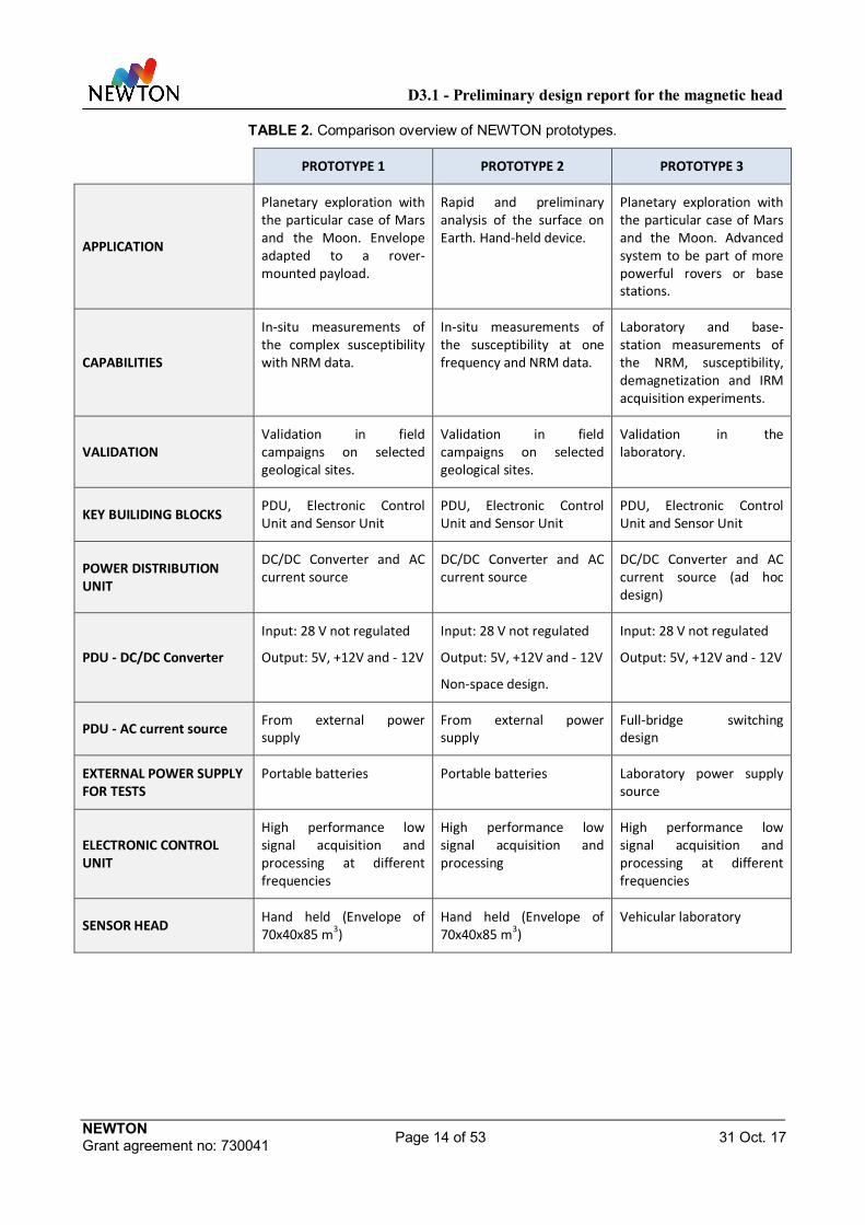
TABLE 2. Comparison overview of NEWTON prototypes.
PROTOTYPE 1 PROTOTYPE 2 PROTOTYPE 3
APPLICATION
Planetary exploration with the particular case of Mars and the Moon. Envelope adapted to a rover-mounted payload.
Rapid and preliminary analysis of the surface on Earth. Hand-held device.
Planetary exploration with the particular case of Mars and the Moon. Advanced system to be part of more powerful rovers or base stations.
CAPABILITIES
In-situ measurements of the complex susceptibility with NRM data.
In-situ measurements of the susceptibility at one frequency and NRM data.
Laboratory and base-station measurements of the NRM, susceptibility, demagnetization and IRM acquisition experiments.
VALIDATION Validation in field campaigns on selected geological sites.
Validation in field campaigns on selected geological sites.
Validation in the laboratory.
KEY BUILIDING BLOCKS PDU, Electronic Control Unit and Sensor Unit
PDU, Electronic Control Unit and Sensor Unit
PDU, Electronic Control Unit and Sensor Unit
POWER DISTRIBUTION UNIT
DC/DC Converter and AC current source
DC/DC Converter and AC current source
DC/DC Converter and AC current source (ad hoc design)
PDU - DC/DC Converter
Input: 28 V not regulated
Output: 5V, +12V and - 12V
Input: 28 V not regulated
Output: 5V, +12V and - 12V
Non-space design.
Input: 28 V not regulated
Output: 5V, +12V and - 12V
PDU - AC current source From external power supply
From external power supply
Full-bridge switching design
EXTERNAL POWER SUPPLY FOR TESTS
Portable batteries Portable batteries Laboratory power supply source
ELECTRONIC CONTROL UNIT
High performance low signal acquisition and processing at different frequencies
High performance low signal acquisition and processing
High performance low signal acquisition and processing at different frequencies
SENSOR HEAD Hand held (Envelope of 70x40x85 m3)
Hand held (Envelope of 70x40x85 m3)
Vehicular laboratory
D3.1 - Preliminary design report for the magnetic head
NEWTON Grant agreement no: 730041 Page 15 of 53 31 Oct. 17
3. PRELIMINARY DESIGN AND OPTIMIZATION OF THE MAGNETIC HEAD
3.1. PROTOTYPE 1 AND 2
3.1.1. General operational requirements
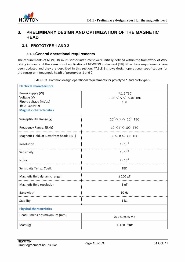
The requirements of NEWTON multi-sensor instrument were initially defined within the framework of WP2 taking into account the scenarios of application of NEWTON instrument [18]. Now these requirements have been updated and they are described in this section. TABLE 3 shows design operational specifications for the sensor unit (magnetic head) of prototypes 1 and 2.
TABLE 3. Common design operational requirements for prototype 1 and prototype 2.
Electrical characteristics
Power supply (W) Voltage (V) Ripple voltage (mVpp) (f: 0 - 30 MHz)
≤1.5 TBC 5 .00 ≤ V ≤ 5.40 TBD
150
Magnetic characteristics
Susceptibility Range (χ) 10-6≤χ≤ 103 TBC
Frequency Range: f(kHz) 10 ≤ f ≤ 100 TBC
Magnetic Field, at 3 cm from head: B(μT) 30 ≤ B ≤ 300 TBC
Resolution 1 · 10-6
Sensitivity 1 · 10-6
Noise 2 · 10-7
Sensitivity Temp. Coeff. TBD
Magnetic field dynamic range ± 200 µT
Magnetic field resolution 1 nT
Bandwidth 10 Hz
Stability 1 ‰
Physical characteristics
Head Dimensions maximum (mm) 70 x 40 x 85 m3
Mass (g) ≤400 TBC

D3.1 - Preliminary design report for the magnetic head
NEWTON Grant agreement no: 730041 Page 16 of 53 31 Oct. 17
3.1.2. General design requirements
The architecture is divided into three blocks: the power and control units will be allocated inside the rover body, and the Sensor Unit will be deployed to ground. Therefore, the environmental requirements are only applicable to the sensor unit. TABLE 4 shows the environmental requirements for the SU of prototype 1.
TABLE 4. Design requirements for the SU of prototype1.
Temperature
Operating: T(°C)
Storage: T(°C)
-40 ≤ T ≤ 110 TBC
-150 ≤ T ≤ 80 ; Relative humidity ≤ 90 % TBC
Air cleanliness class at least 8 of ISO to GOST ISO 14644-1-2002
Environmental
Vibration Low-sine sweep: 5Hz to 1000 Hz at 2 oct / min 0.5g for each axis (worst case)
Sine: 5Hz to 100 Hz at 2 oct / min 5g for each axis (worst case)
Random: f = 5 - 2000 Hz 0.1g2/Hz (worst case)
The instrument must not have resonant frequencies less than 40 Hz (Exomars 2020 launcher requirement).
Shock Frequency, Hz From 30-50 To 2000-5000
Acceleration, g 15-40 1000
Thermal vacuum Cycles from -55ºC to 70ºC, 10-6 mbar 6 cycles TBC
Radiation
Components Flight model (rad hardened capacitors and resistors) immune to radiation.
3.1.3. Working principle Prototypes 1 and 2 sensor head consists of two elements: the susceptometer system and a magnetometer.
The susceptometer is one of the main objectives of the project and the working principle is described in detail in this section.
The magnetometer considered for prototypes 1 and 2 is a three axes magnetometer based on anisotropic magneto resistance (AMR), based on AMR instrument of Exomars 2020 as explained in the proposal.
In this project HMC2003 commercial magnetometer (by Honeywell) will be used. This device has the transducers HMC1001 (one axis magnetometer) and HMC1002 (two axes magnetometer) and it has an

D3.1 - Preliminary design report for the magnetic head
NEWTON Grant agreement no: 730041 Page 17 of 53 31 Oct. 17
electronic control system already integrated. HMC1001 and 1002 are robust against the radiation environment expected on the surfaces on Mars and the Moon[20]. The electronic circuitry is not prepared for planetary surface conditions but it can be easily replaced by equivalent rad hardened and wide temperature components. A more reduced size alternative is to consider the small size 2-Axis Magnetic Sensor Circuit HMC6042, or the analog solution Integrated Compass Sensor HMC6052. The HMC6052 presents a 3.5 x 3.5 x 0.8 mm 14-pin LCC package with a resolution of 5 V/mT and a -0.2 mT to +0.2 mT full scale field range. The HMC6042 incorporates an ASIC DIE amplifier, providing a -0.6 mT to +0.6 mT full scale field range and a resolution of 0.1 mV/V/mT, with a total envelope size of 5 x 3.6 x 1.0mm in a LCC Surface Mount Package.
The susceptometer system, designed to achieve the requirements depicted in section 3.1.1, consist of a modified tank circuit (FIGURE 4), in which it is included the ferrite core (L) as a self-inductance in the resonatingloop.
The circuit is composed by the inductance (L) in series with a capacitor (C2) and both in parallel with a capacitor C1 .In the present design: C1 = C2 = C.
FIGURE 4. Modified tank circuit scheme.
This circuit has two resonant frequencies:
=√
(3.1-1)
= (3.1-2)
In the second one, f02, it is achieved a maximization of the rate current circulating in the resonant loop to the input current. This guarantees a moderate to high current in the circuit with a low power consumption from the power supply. Themoderate to high current value in the resonant loop will be used to produce a sufficiently intense stray field in the open part of the ferrite core to magnetize the rocks or soil.
The self-inductance is a double magnetic circuit. It is an active part consisting of a H shape ferrite core coiled with primary coils carrying the resonant loop current, and secondary pick-up coils, which will measure the change of the magnetic flux in the magnetic circuit (FIGURE 5).
One of the magnetic circuits is open to the air and serves as a reference permeability or susceptibility. The other magnetic circuit is open in the absence of rock or soil sample and it is closed when the sample is approached to the free ends of the ferrite.

D3.1 - Preliminary design report for the magnetic head
NEWTON Grant agreement no: 730041 Page 18 of 53 31 Oct. 17
FIGURE 5. H-shaped ferrite core of the susceptometer’s sensor head.
Prototypes 1 and 2determine both components of the complex susceptibility (real and imaginary components) in a range of frequencies or at a single frequency respectively.
Real part determination
Option 1. Frequency shifting.
The closure of this magnetic circuit with a sample with a permeability (μ) or susceptibility (Χ, μ=1+Χ) different to that of the air changes the self-inductance of the core and therefore, the resonance frequency of the electrical circuit.
The real part of the permeability or susceptibility of the sample is derived from the measurement of the two resonance frequencies: with and without the sample.
The resonance seeking procedure is as follows: prior to the sample approach, the circuit is symmetric, being the four free ends of the ferrite in contact to the air. In this configuration the resonance frequency is determined when the input current (determined as Iin = (Vin – Vs)/Rin measuring the difference of voltage) is minimized during the sweep. The phase in this condition is set as the zero phase. When the sample is approached to the ferrite closing one of the magnetic circuits, the resonance frequency is determined because it zeroes the phase, i.e. in the new resonance frequency, which is possible when the relative permeability of the sample is much smaller than that of the ferrite core (μr sample <<μr ferrite). This is a reasonable approximation when measuring natural samples and the manufactured samples prepared for the calibration.
The calculation of the real susceptibility for this option is as follows:
First, the value of the resonance frequency is related with the self-inductance of the susceptometer core.

D3.1 - Preliminary design report for the magnetic head
NEWTON Grant agreement no: 730041 Page 19 of 53 31 Oct. 17
From(3.1-2) it is calculated the resonance frequency of the circuit: = ⋅⋅
. For this calculation we
distinguish between two resonance frequencies: without (f0) and with (f’) sample.
= ⋅⋅
(3.1-3)
f'=1
2π⋅
2L'⋅C
(3.1-4)
Where L0 and L’ are the self-inductances of the core without and with sample respectively.
Then, the self-inductance is related with the magnetic susceptibility of the ferrite core and the sample by means of the circulation of the magnetic flux within the core, i.e. solving the magnetic circuit. This calculation is done for both situations: with and without sample.
The self-inductance depends on the magnetic flux (eq. 5) and this depends at the same time on the relative permeability (eq. 6) straightforwardly related with the magnetic susceptibility.
= = (3.1-5)
Where is the magnetic flux, n is the number of turns of the primary coil, Iis the current through the coil and Ri is the reluctance. The reluctance is in a magnetic circuit the analogous to the resistance in an electric circuit, and it is related with the relative permeability of the materials.
=1
(3.1-6)
Where li is the length of the path, Si the surface section of the path and µi the real magnetic permeability of the path’s material (µ0 for free space µf for the ferrite µs for the sample).
A quick analysis of the electrical circuit in terms of the self-inductance as function of a complex reluctance based on a complex permeability shows that the resonance frequency, as it is the frequency where the imaginary component of the impedance vanishes, does not present contribution of the imaginary component of the permeability. Given this fact, in the following analysis we will refer to only the real component of the permeability (and thus, the susceptibility) as we are working always in the resonance frequency.
Eq. (3.1-6) presents the reluctance of each part of the path of the magnetic circuit formed by the H ferrite core and either air or sample. The magnetic circuit formed by the susceptometer and the sample can be solved in terms of this relations. Substituting the self-inductance for its relation in terms of the magnetic permeability in the expression for the resonance frequency, it can be found the expression that relates the resonance frequency with the relative permeability of the sample under measurement:
= ⋅· ·
·
(3.1-7)

D3.1 - Preliminary design report for the magnetic head
NEWTON Grant agreement no: 730041 Page 20 of 53 31 Oct. 17
(3.1-7) represents the resonance frequency for the circuit with no sample in terms of the permeability of the materials, and an equivalent expression can be found for the scenario with the studied sample which relates the resonance frequency f’ with the real permeability µ’ of the sample. Relating these expressions, solving for µ’, and then substituting the permeability µsr’ by its expression in terms of the susceptibility: µsr’= χs – 1, it is found the following expression:
=− ′
′ − (3.1-8)
(3.1-8) represents the relation between the real susceptibility of the sample and the resonance frequency of the circuit in the different measurement conditions. To generate an absolute value, the device must be calibrated and the results must be inter-compared with those from calibrated devices.
Option 2. Magnetic flux variation in the secondary coils.
The effect of the rock or soil approaching the ferrite core changes the magnetic induction and therefore, the electromotive force, which can be recorded by the secondary coils. This measurement in amplitude and phase of the magnetic induction in the ferrite arms provides information about the magnetic properties of the sample under measurement.
The permeability is derived from the measurement of the difference in the magnetic flux in the secondary coils. This measurement is done differentially, i.e. the secondary coil by the sample is in series-opposition with the one facing the air to improve sensitivity.
In this case the theoretic are simpler but the results are more complicated due to the complex contributions of the different factors taken into account.
The secondary coils behave as pick-up coils which produce an electromotive force given by Faraday’s law:
= −Φ
(3.1-9)
Which means, that voltage difference (i.e. the electromotive force ) induced in the secondary coils is the derivative of the magnetic flux with respect to the time and multiplied by minus and the number of turns of the secondary coil.
Then the objective is to relate this voltage signal, easily measured with a lock-in amplification given that the excitation is a sinusoidal magnetic field, with the magnetic susceptibility of the sample under measurement.
To do that, the magnetic flux within the secondary coils must be calculated by means of the solution of the magnetic circuit, and then related with the magnetic susceptibility using the relation between magnetic field and magnetic induction. The main equation for a magnetic circuit says:
· = ( · ) (3.1-10)
Where N·I represents the magnetomotive force induced in the magnetic circuit (N = number of turns of the primary coil, I = current through this coil), and “i” is an index that represents each of the different paths of the circuit (ferrite, air, and/or sample).
D3.1 - Preliminary design report for the magnetic head
NEWTON Grant agreement no: 730041 Page 21 of 53 31 Oct. 17
To solve the magnetic circuit a number of considerations must be taken into account:
1. Conservation of magnetic induction B. In the interfaces ferrite/air and ferrite/sample the perpendicular magnetic induction must follows the Maxwell law for magnetism·B = 0, which means that the magnetic field H either within the ferrite and in the air/sample can be calculated and are related with the permeability, as B = µ·H (or from the magnetization M = χ·H, where B = µ0·(H+M)).
2. The susceptibility is a complex value (χ’+iχ’’), but as we are studying natural samples where the value of the imaginary component is χ’’<< χ’, we take advantage of this fact and can simplify in the calculations of the real component.
3. The areas of the cross-sections are similar in all the cases. This is a reasonable approximation due to the geometry and size of the susceptometer head.
The magnetic field is found in the different paths of the circuit in the different scenarios (with and without sample). With this, it is possible to calculate the magnetic induction Bf in the ferrite and the magnetic flux which excites the secondary coil in terms of the susceptibility of the materials.
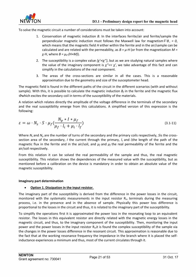
A relation which relates directly the amplitude of the voltage difference in the terminals of the secondary and the real susceptibility emerge from this calculations. A simplified version of this expression is the following:
= · · · (∗ ∗
· + ·) (3.1-11)
Where Ns and Np are the number of turns of the secondary and the primary coils respectively, Sis the cross-section area of the secondary, I the current through the primary, ls and lithe length of the path of the magnetic flux in the ferrite and in the air/soil, and µf and µf the real permeability of the ferrite and the air/soil respectively.
From this relation it can be solved the real permeability of the sample and thus, the real magnetic susceptibility. This relation shows the dependences of the measured value with the susceptibility, but as mentioned before a calibration on the device is mandatory in order to obtain an absolute value of the magnetic susceptibility.
Imaginary part determination
Option 1. Dissipation in the input resistor.
The imaginary part of the susceptibility is derived from the difference in the power losses in the circuit, monitored with the systematic measurements in the input resistor Rin terminals during the measuring process, i.e. in the presence and in the absence of sample. Physically this power loss difference is proportional to the losses in the circuit and thus, it is related to the imaginary part of the susceptibility.
To simplify the operations first it is approximated the power loss in the resonating loop to an equivalent resistor. The losses in this equivalent resistor are directly related with the magnetic energy losses in the magnetic circuit, and thus, to the imaginary component of the susceptibility. Then, monitoring the input power and the power losses in the input resistor Rinit is found the complex susceptibility of the sample via the changes in the power losses difference in the resonant circuit. This approximation is reasonable due to the fact that at the working resonance frequency the impedance in the branch where it is placed the self-inductance experiences a minimum and thus, most of the current circulates through it.

D3.1 - Preliminary design report for the magnetic head
NEWTON Grant agreement no: 730041 Page 22 of 53 31 Oct. 17
Given that there is no available data for the imaginary susceptibility of the measured samples, the calibration was not possible. However, a normalized value for the imaginary susceptibility evaluated from the power losses difference has been done and presented in Section 4.2, FIGURE 30.
Option 2. Magnetic flux variation in the secondary coils.
An alternative method through the measurement in the secondary coils is based on the change of the phase, directly related with the losses of the sample and thus, with the imaginary component of the susceptibility.
One of the secondary coils is placed on the upper part of the H ferrite core, always facing the air and considered as reference value. The other one is placed in one of the lower arms, close to the edge of the ferrite core. When a sample with a complex susceptibility approaches, an in-phase quadrature measurement reveals the amplitude and phase changes of the electromotive force in this secondary coils. While the amplitude is related with the value of the real component of the susceptibility as we have seen before, the phase is related with both real and imaginary components. Then, the imaginary component can be calculated if we have a previous value of the real component.
The in phase quadrature technique (lock-in amplification) measures the amplitude (R) and phase (θ),or its equivalent real (X) and imaginary (Y) projections in the complex plane, of a signal at a certain frequency, that in this case is the electromotive force from the upper secondary. These signals respond to the relations:
tan = (3.1-12)
= √ + (3.1-13)
For this technique the signals are returned by the lock-in amplifier as a differential voltage signal, product of the subtraction of the reference signal to the measuring signal. While the real component (X) of the response can be directly related to the real susceptibility, the imaginary component (Y) of this signal with the imaginary susceptibility has contributions of both real and imaginary susceptibility (and other factors) in a complex relation. Prior to the calculation of the imaginary susceptibility it is mandatory the determination of the real susceptibility and a fine calibration of the instrument.
This technique is being currently under development and therefore there are not experimental results at this stage. Equations relating the X and Y signals with the complex susceptibility are obtained solving the magnetic circuit in an analogue exercise to the one done in the real part, but with more complex relations. These relations are not presented on this section as there is a refinement to be done on the current status of the theory for these calculations.
In this preliminary design two options are proposed for each component. TABLE 5 summarises advantages and disadvantages of the different options.
TABLE 5. Summary of advantages and disadvantages of the different methodologies taken into account in the preliminary design.
Parameter Measuring method Advantages Disadvantages
Χ’ Option 1 Frequency measurement. High resolution.
Easy derivation of the measured
For prototype 1. Loss of resolution for increasing frequencies (See section 3.1.5)

D3.1 - Preliminary design report for the magnetic head
NEWTON Grant agreement no: 730041 Page 23 of 53 31 Oct. 17
magnitude
Option 2 Simplicity in the design. Secondary coils serve for both parameters to be measured.
Amplitude measurement. Poorer resolution than frequency measurement.
Χ”
Option 1 Easy measurement. Difficult derivation of the parameter.
Option 2 Simplicity in the design. Secondary coils serve for both parameters to be measured.
Difficult phase measurement. Multiple monitoring points.
3.1.4. Design of the Magnetic Head The magnetic head is allocated in the sensor unit. It consists of the susceptometer and magnetometer heads. Apart from this, the sensor unit contains the proximity electronic, which has to be close to the sensors. The preliminary design of the box is shown in FIGURE 6.
FIGURE 6.Preliminary design of the sensor unit of NEWTON prototypes 1 and 2. The dimensions are 60x40x70 m3. The sensor unit contains the susceptometer head (H self-inductance, the two capacitors, the resistor and the magnetic amplifier in prototype 1) and the magnetometer as well as two electronic PCBs for the proximity electronic (reading and exciting).
The susceptometer is based on a parallel resonant circuit, with an induction due to the H shape ferrite core and two capacitors connected in series and in parallel with the coil. The electrical circuit is very robust to the environment and therefore, it might be used as heater prior to the measurements to achieve temperatures > -45 ºC.

D3.1 - Preliminary design report for the magnetic head
NEWTON Grant agreement no: 730041 Page 24 of 53 31 Oct. 17
The H shaped ferrite core (FIGURE 5) will be constructed with two U-cores glued together with minimal airgap in the junction, or separated with a stack of several layers of soft ferromagnetic and non-magnetic conductor films to avoid interconnection.
The core of the ferromagnetic material is subjected to an alternating magnetizing force; for each cycle of the magnetic force a hysteresis loop is traced out and some part of the magnetic energy of the ferromagnetic material is lost in the circuit. Hysteresis loss is proportional to the maximum magnetic field applied Bmax, to the frequency of the field f and to the volume of the ferromagnetic material. To minimize hysteresis loses, the ferrite material is chosen to be a soft ferromagnetic ferrite with very low coercivity.
A low value in the coercive field and in the imaginary component of the ferrite core permeability is mandatory when considering the materials for the construction of the prototypes 1 and 2.
Main features and characteristics, with the range of values permitted in the selection of the ferrite properties are detailed in TABLE 6.
TABLE 6. Requirements for the susceptometer ferrite core
Ferrite core requirements (at laboratory conditions: P = 1 atm, T = 298 k)
Characteristic Required value Current value
Real Relative Permeability (µr) 1000 - 5000 2000
Imaginary Relative Permeability (µr‘) ≤10 < 10
Frequency Range (linear response) ≤ 100 kHz ≤ 1000 kHz
Saturation Flux density > 300 mT 500 mT
Coercive Field Strength < 20 A/m 14 A/m
Loss Factor Density < 100 mW/cm3 80mW/cm3
Curie Temperature > 180 ºC (Space req.) > 220 ºC
Resistivity > 2 Ω·m 5 Ω·m
The primary winding is made with a number of turns between 5 and 10 turns per arm (current prototypes for testing have 7 and 10 turns), depending on the wire diameter and ferrite arm’s length. The windings in the four arms are connected in series so that the magnetic induction in the junction is minimized to avoid saturation of the ferrite, and the magnetic flux creates a closed loop on half of the ferrite core (upper and lower size).
Previous models were based on a single U shaped ferrite but they did not permit to extract absolute values of the susceptibility since the measurement is not differential. More details of the optimization are described in section 3.1.6.
At high frequencies the current is concentrated near the surface of the conductor (skin effect) and the resistance increases. The penetration depth of the skin effect is approximated by: ≈
With: f = frequency;
D3.1 - Preliminary design report for the magnetic head
NEWTON Grant agreement no: 730041 Page 25 of 53 31 Oct. 17
permeability: μ= μr⋅μo , with μo = 4⋅ ⋅10-7 (H/m) permeability of free space. σ=conductivity or resistivity ρ=1/σ=1.72⋅10-8 Ωm for copper.
In the case of copper at 50Hz, 10kHz, 100kHz are δ = 9.22, 0.65 and 0.21 mm respectively. Since the working frequencies will be in the range of 10-100kHz it will be considered the use of Litz wire, which assures that the diameter does not exceed 2⋅δ = 0.42mm.
Winding losses are due to resistance of the copper and can be reduced by using Litz wire, but the cross-sectional reduction can increase the losses. Experimental results for different types of wire (monofilament copper, Litz wire of different diameters) have shown that at the working frequencies the contribution of skin effect losses is negligible.
The diameter of the wire must be between 0.6 mm and 1 mm, either monofilament copper or Litz wire. The estimated length of the total wire would be around 1 meter maximum, with a total resistance of 0.2 Ω. In the case of using Litz wire, it is foreseen the following constructions: 0.675 mm, 0.875mm or 1.05mm total diameter with 3, 5 or 7 sub-bundles respectively, with 28 strands each sub-bundle. Similar Litz wire constructions will be equally valid, if and when the total diameter of the wire is on the proposed range and the strand diameter is small enough to prevent the formation of Eddy currents.
The secondary coils are coiled near the free ends in the left (or right) upper and lower arms of the ferrite. They are made of monofilament copper wire of a maximum diameter of 0.5 mm. They should be made of maximum 10 turns and connected to high impedance inputs in order to avoid mutual inductance.
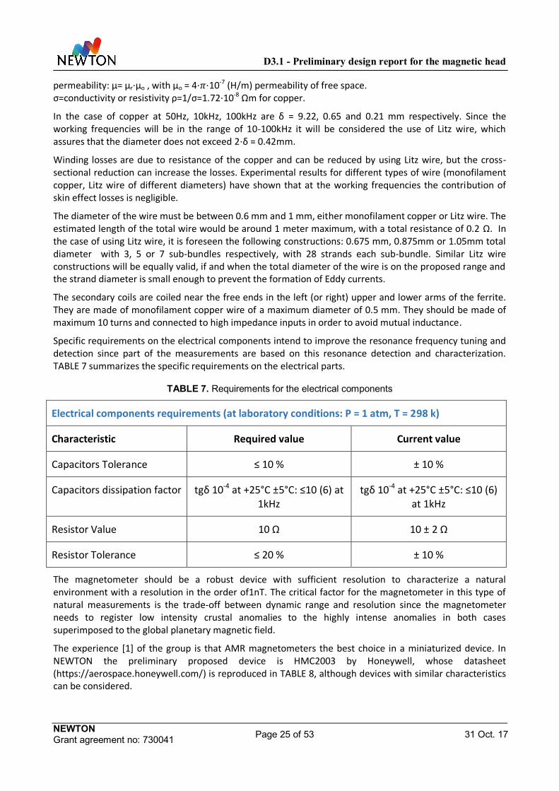
Specific requirements on the electrical components intend to improve the resonance frequency tuning and detection since part of the measurements are based on this resonance detection and characterization. TABLE 7 summarizes the specific requirements on the electrical parts.
TABLE 7. Requirements for the electrical components
Electrical components requirements (at laboratory conditions: P = 1 atm, T = 298 k)
Characteristic Required value Current value
Capacitors Tolerance ≤ 10 % ± 10 %
Capacitors dissipation factor tgδ 10-4 at +25°C ±5°C: ≤10 (6) at 1kHz
tgδ 10-4 at +25°C ±5°C: ≤10 (6) at 1kHz
Resistor Value 10 Ω 10 ± 2 Ω
Resistor Tolerance ≤ 20 % ± 10 %
The magnetometer should be a robust device with sufficient resolution to characterize a natural environment with a resolution in the order of1nT. The critical factor for the magnetometer in this type of natural measurements is the trade-off between dynamic range and resolution since the magnetometer needs to register low intensity crustal anomalies to the highly intense anomalies in both cases superimposed to the global planetary magnetic field.
The experience [1] of the group is that AMR magnetometers the best choice in a miniaturized device. In NEWTON the preliminary proposed device is HMC2003 by Honeywell, whose datasheet (https://aerospace.honeywell.com/) is reproduced in TABLE 8, although devices with similar characteristics can be considered.

D3.1 - Preliminary design report for the magnetic head
NEWTON Grant agreement no: 730041 Page 26 of 53 31 Oct. 17
TABLE 8. 3-Axis Magnetic Sensor Hybrid HMC20031
Characteristics Conditions Min Typ Max Units
Magnetic Field
Dynamic range 4nTto ± 0.2 mT ±4nT ±0.2 mT Sensitivity 9.8 10 10.2 V/mT
Null Field Output 2.3 2.5 2.7 V Resolution 4 mT Field Range Maximum Magnetic Flux
Density -0.2 0.2 mT
Output Voltage Each Magnetometer Axis Output
0.5 4.5 V
Bandwidth 1 kHz
Errors
Linearity Error 0.1 mT Applied Field Sweep 0.2 mT Applied Field Sweep
0.5 1
2 2
%FS
Hysteresis Error 3 Sweeps across 0.2 mT 0.05 0.1 %FS Repeatability Error 3 Sweeps across 0.2 mT 0.05 0.1 %FS
Power Supply Effect PS Varied from 6 to 15V With 0.1 mT Applied Field
Sweep
0.1 %FS
Offset Strap
Resistance 10.5 ohms Sensitivity 465 475 485 mA/mT
Current 200 mA
Set/Reset Strap
Resistance 4.5 6 ohms Current 2 us pulse, 1% duty cycle 3.0 3.2 5 amps
Tempcos
Field Sensitivity -600 ppm/°C Null Field Set/Reset Not Used
Set/Reset Used 400
100 ppm/°C
Environments
Temperature Operating Storage
-40 -55
- -
+85 +125
°C °C
Shock 100 g Vibration 2.2 g rms
Electrical
Supply Voltage(3) 6 15 VDC
1 Source: https://aerospace.honeywell.com/
D3.1 - Preliminary design report for the magnetic head
NEWTON Grant agreement no: 730041 Page 27 of 53 31 Oct. 17
Supply Current 20 mA (1) Unless otherwise stated, test conditions are as follows: Power Supply = 12VDC, Ambient Temp = 25°C, Set/Reset switching is active (2) Units: 1 gauss = 0.1 mT (3) Transient protection circuitry should be added across V+ and Gnd if an unregulated power supply is used.
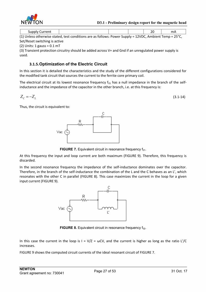
3.1.5. Optimization of the Electric Circuit In this section it is detailed the characteristics and the study of the different configurations considered for the modified tank circuit that sources the current to the ferrite core primary coil.
The electrical circuit at its lowest resonance frequency f01 has a null impedance in the branch of the self-inductance and the impedance of the capacitor in the other branch, i.e. at this frequency is:
LC ZZ (3.1-14)
Thus, the circuit is equivalent to:
FIGURE 7. Equivalent circuit in resonance frequency f01.
At this frequency the input and loop current are both maximum (FIGURE 9). Therefore, this frequency is discarded.
In the second resonance frequency the impedance of the self-inductance dominates over the capacitor. Therefore, in the branch of the self-inductance the combination of the L and the C behaves as an L’, which resonates with the other C in parallel (FIGURE 8). This case maximizes the current in the loop for a given input current (FIGURE 9).
FIGURE 8. Equivalent circuit in resonance frequency f02.
In this case the current in the loop is I = V/Z = ωCV, and the current is higher as long as the ratio L’/C increases.
FIGURE 9 shows the computed circuit currents of the ideal resonant circuit of FIGURE 7.

D3.1 - Preliminary design report for the magnetic head
NEWTON Grant agreement no: 730041 Page 28 of 53 31 Oct. 17
FIGURE 9. Currents in the ideal resonant circuit for different input resistances. The input voltage is 1 V. The values of the components are: C=4.7 μF y L=50 μH and the frequency range is from 1 kHz to 100 kHz, for different input resistances R (ohms). The resonant frequencies for such values are t f01=32.8 kHz and fo2=46.4 kHz. As it can be seen the input current is maximum at f01 and minimum at f02; for that reason the second one is chosen.
The range of this current is limited between the current needed to create enough stray field to perform the measurements and the saturating field of the ferrite. However, due to the high demagnetizing factor of the H-shaped ferrite, the current limit is beyond the working currents considered for these prototypes (up to 6 A, and below 1 A as nominal value).
We consider a target range of frequency from 10 to 100 kHz to measure susceptibility of most of the minerals. FIGURE 10 shows the impedance values (μH) needed to have resonances at a range of frequencies in kHz) for different capacitors.
100
101
1020
0.2
0.4
0.6
0.8
1
1.2
1.4
Rp=0
Rp=0.4
Rp=0.8
Rp=1.2
f1=10.3 f2=14.6
f(kHz)
|I(A
)|
Corrientes en el circuito resonante paralelo-serie con pérdidas en Rp(). V=1v. R=1 , C=4.7F, L=50H
Ii(A)Ic(A)Icl(A)

D3.1 - Preliminary design report for the magnetic head
NEWTON Grant agreement no: 730041 Page 29 of 53 31 Oct. 17
FIGURE 10. Inductance versus resonant frequency for different capacitors values
In the preliminary design, which has been exhaustively tested, it was given a fixed value for the self-inductance and selected values for the capacitors to produce a great current through the primary coil at the working resonance frequency. To work at a different frequencies preserving the low power consumption vs the high current in the sensor loop, and taking into account that the value of the self-inductance cannot be modified, the value of the capacitor must be modified in accordance with the new desired resonance frequency. So that, to work at three different discrete frequencies, requires a set of three different branches of capacitors and an additional switching system (FIGURE 11). This technique presents a series of inconvenient in terms of volume, mass and electronics and more importantly, of loss of robustness. Any additional set of capacitors increases the mass and volume of the complete system, what difficult its miniaturization and adaptation to portable devices. Besides that, to select the different capacitors set it is needed a switching system with relays capable to tolerate the current, which are usually magnetic relays with a considerable size and weight.
10 20 30 40 50 60 70 80 90 100100
101
102
10.0
325.3
640.5
955.81271.1
1586.31901.62216.82532.12847.43162.63477.93793.2
4108.44423.7
4738.9
5054.2
5369.5
5684.7
6000.0
f(KHz)
L(
H)
INTA-19-Sep-2017
10.0nF325.3nF640.5nF955.8nF1271.1nF1586.3nF1901.6nF2216.8nF2532.1nF2847.4nF3162.6nF3477.9nF3793.2nF4108.4nF4423.7nF4738.9nF5054.2nF5369.5nF5684.7nF6000.0nF

D3.1 - Preliminary design report for the magnetic head
NEWTON Grant agreement no: 730041 Page 30 of 53 31 Oct. 17
FIGURE 11. Block diagram of the susceptometer at the proposal level. In the part of the resonant circuit it can be seen that it is foreseen three branches to accomplish the measurements in the desired frequency
range.
To avoid these inconvenient, it is considered the following construction of the sensor head:
The objective is to have a varying self-inductance in the resonant circuit and use this variability to tune the resonance at different frequencies. This question is achieved by means of the introduction of a magnetic amplifier ([20] and [21]). A magnetic amplifier is a magnetic circuit with a double winding (FIGURE 12): one winding carries AC current, the other winding is connected to a DC power supply which injects DC current into the winding. This current changes the permeability of the core in such a way that it can modulate the amplitude of the AC current for a certain power supply. In NEWTON design, the DC current is used to change the permeability and therefore, the self-inductance and its resonance with the capacitors. FIGURE 13A shows the scheme of the resonant circuit with the magnetic amplifier.
FIGURE 12. Two cores magnetic amplifier scheme.
FIGURE 13. A. Resonant circuit with magnetic amplifier. B. Didactical scheme of connections (without H-
shaped ferrite).

D3.1 - Preliminary design report for the magnetic head
NEWTON Grant agreement no: 730041 Page 31 of 53 31 Oct. 17
Experimental results have proven that including a magnetic amplifier in the ferrite core branch can produce a sweep in the resonant frequency within the range of 10 to 100 kHz, varying current Idc from 30mA to 300mA. This technique allows to perform measurements with the susceptometer within this range in a continuous sweep of frequency values.
The advantage is the capability to achieve a continuous range of frequency for the susceptibility measurements.
The main drawback is the progressive decrease in sensitivity when frequency shifts are measured to derive the susceptibility. Because of this, the alternative method of measuring the magnetic flux with the secondary coils of the H shape ferrite core is implemented. Both principles will be developed in parallel and best solution will be used for the construction of the advanced prototype 1. In the case of prototype 2, it will be studied whether the incorporation or not of the magnetic amplifier is beneficial for a hand-held, fast and preliminary study device, as a function of the decrease in the resolution and the quantity of information achievable with the different configurations.
In case of the use of one single capacitors value together with the magnetic amplifier, there has been measured a frequency sweep up to 40 kHz. FIGURE 14 and FIGURE 15 show frequency versus current and induction for different size toroids and windings. FIGURE 16B is a photograph of one of the tested circuit, with the magnetic amplifier.
FIGURE 14. Response in frequency (kHz) with the continuous current (mA) and different toroids and windings.
0 200 400 600 800 1000 1200 1400 1600 1800 20000
20
40
60
80
100
120
frec
uenc
ia (k
Hz)
i(mA)
Resonant circuit: w=sqrt(2/(LC)),C=4.7F, with magnetic amplifier(2 toroids.r=5500)
Ndc=60,Nac=30, Ø42xØ26x13mmNdc=60,Nac=10, Ø42xØ26x13mm,Ndc=60,Nac=5, Ø42xØ26x13mmNdc=50,Nac=5, Ø20xØ10x7mmNdc=45,Nac=5, Ø16xØ9.6x6.3mm

D3.1 - Preliminary design report for the magnetic head
NEWTON Grant agreement no: 730041 Page 32 of 53 31 Oct. 17
FIGURE 15. Inductance L (μH) with current Idc (mA) for different toroids and windings.
In the investigation to optimize the electrical circuit, other configurations with different magnetic amplifiers have been proved. Despite of the fact that the other configurations have been rejected, this part of the investigation is summarized in the following for completeness and to serve as a guide for future users. Among the most promising configurations there are two, whose characteristics are summarized below:
Iron powder toroids:
These toroids have low relative permeability (μr). This is appealing since the range to saturation is large. However, the currents needed to reach the whole range are very high and the consumption of the device would exceed the specifications.
Metglastoroids:
Amorphous stripes of Metglas have in contrast very high permeability (FIGURE 16A). Toroids of Metglas were manufactured in the laboratory, mounted (FIGURE 16B) and tested. Its high permeability together with the fact that the permeability varies notably with frequency (FIGURE 17) makes it very difficult to tune the resonance and to detect the frequency, which is needed for measuring.
0 200 400 600 800 1000 1200 1400 1600 1800 200010
-1
100
101
102
103
104
I(mA)
L(uH
)Resonant circuit: w=sqrt(2/(LC)),C=4.7F, with magnetic amplifier(2 toroids.r=5500)
Ndc=60,Nac=30, Ø42xØ26x13mmNdc=60,Nac=10, Ø42xØ26x13mm,Ndc=60,Nac=5, Ø42xØ26x13mmNdc=50,Nac=5, Ø20xØ10x7mmNdc=45,Nac=5, Ø16xØ9.6x6.3mm

D3.1 - Preliminary design report for the magnetic head
NEWTON Grant agreement no: 730041 Page 33 of 53 31 Oct. 17
FIGURE 16. A.Hysteresis cycles wit different METGLAS treatment. The toroids were performed with no field
annealed stripes B. Toroids of Metglas corefor the construction of the magnetic amplifier.
FIGURE 17. Amplifier core real permeability and losses with frequency (METGLAS 2826MB). Manufacturer
parameters reproduced to assist the explanation (www.tridelta.de, www.ferroxcube.com).
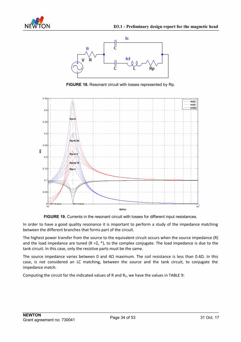
An important factor when analysing the modified tank circuit is the power losses. This losses, as we saw previously, could be due to the hysteresis losses or induced Eddy currents in the conductors of the circuit. The losses produced in the self-inductance (L + Lac) can be modelled by an additional series resistor in the resonating branch of the circuit.
In FIGURE 18 it is shown the resonant circuit considering losses represented by Rp due to several factors like the skin effect, inductance winding, the hysteresis loop of the ferrite (B-H loop) and Eddy currents.
D3.1 - Preliminary design report for the magnetic head
NEWTON Grant agreement no: 730041 Page 34 of 53 31 Oct. 17
FIGURE 18. Resonant circuit with losses represented by Rp.
FIGURE 19. Currents in the resonant circuit with losses for different input resistances.
In order to have a good quality resonance it is important to perform a study of the impedance matching between the different branches that forms part of the circuit.
The highest power transfer from the source to the equivalent circuit occurs when the source impedance (R) and the load impedance are tuned (R =ZL *), to the complex conjugate. The load impedance is due to the tank circuit. In this case, only the resistive parts must be the same.
The source impedance varies between 0 and 4Ω maximum. The coil resistance is less than 0.4Ω. In this case, is not considered an LC matching, between the source and the tank circuit, to conjugate the impedance match.
Computing the circuit for the indicated values of R and RP, we have the values in TABLE 9:
101
102
0
0.05
0.1
0.15
0.2
0.25
0.3
0.35
0.4
0.45
Rp=0
Rp=0.25
Rp=0.5
Rp=0.75
Rp=1
f01=10.3kHz f02=14.6kHz
f(kHz)
I(A)
Ie(A)Ic(A)Icl(A)
D3.1 - Preliminary design report for the magnetic head
NEWTON Grant agreement no: 730041 Page 35 of 53 31 Oct. 17
TABLE 9. Input current: Ii (A) for different values of R and RP.
R(Ω)Rp (Ω) 0 0.2 0.4
0.1 8 3.5 1
2 0.61 0.54 0.47
4 0.47 0.4 0.35
R is needed to be able to tune the circuit in the detection and Rp is unavoidable but to have the largest current in the loop and the minimum input current the values of the two resistors should be minimized.
3.1.6. Optimization of the Magnetic Head In this section it is described a summary of the experimental tests performed in order to optimize the design of the susceptometer magnetic head.
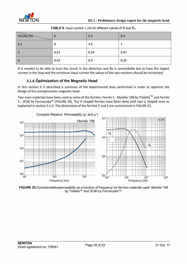
Two main materials have been used as cores of the ferrites: Ferrite 1 - Manifer 198 by TrideltaTM and Ferrite 2 - 3C90 by Ferroxcube™ (FIGURE 20). The H shaped ferrites have been done with two U shaped ones as explained in section 3.1.5. The dimensions of the ferrites 1 and 2 are summarized in FIGURE 21.
FIGURE 20.Complexrelativepermeability as a function of frequency for the two materials used: Manifer 198
by Tridelta™ and 3C90 by Ferroxcube™.

D3.1 - Preliminary design report for the magnetic head
NEWTON Grant agreement no: 730041 Page 36 of 53 31 Oct. 17
FIGURE 21.Physical dimensions of the two ferrites used.
From now on we will focus on three heads with the characteristics described in TABLE 10. The electric circuit’s capacitors to achieve discrete resonances in the range of 10 to 100 kHz and the resonance frequencies obtained are depicted in TABLE 11.
TABLE 10. Magnetic heads characteristics.
Head Name Type of Wire Wire Diameter (mm) Number of turns L (H)
Ferrite 1 Monofilament 1 10 5.28·10-5
Ferrite 2.1 Litz 1 10 5.20·10-5
Ferrite 2.2 Litz 1.5 7 2.80·10-5
TABLE 11. Electrical circuit configurations and resonance.
Configuration Capacitor Value (F) Frequency value (Hz) (theoretical)
Frequency value (Hz) (experimental)
Ferrite 1 3.00·10-7 56.553 56.540
Ferrite 2.1.1 4.30·10-6 15.052 15.170
Ferrite 2.1.2 5.00·10-7 44.141 44.270
Ferrite 2.1.3 1.50·10-7 80.591 86.170
Ferrite 2.2.1 8.00·10-6 15.038 15.100
Ferrite 2.2.2 1.00·10-6 42.535 43,370
Ferrite 2.2.3 3.00·10-7 77.659 82.400
D3.1 - Preliminary design report for the magnetic head
NEWTON Grant agreement no: 730041 Page 37 of 53 31 Oct. 17
The optimization of the head aims two main goals:
1 – Increase of the sensitivity for the imaginary component determination.
2 – Configuration which guarantees the least power consumption with enough resolution in order to achieve the highest efficiency of the electrical circuit in terms of power consumption.
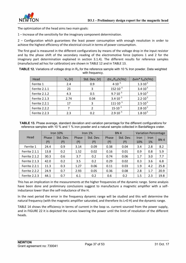
The first goal is measured in the different configurations by means of the voltage drop in the input resistor and by the phase shift of the secondary reading of the electromotive force (options 1 and 2 for the imaginary part determination explained in section 3.1.4). The different results for reference samples (manufactured ad hoc for calibration) are shown in TABLE 12 and in TABLE 13.
TABLE 12. Variations of voltage drop in Rin for the reference sample with 10 % Iron powder. Data weighted with frequency.
Head Vin (V) Std. Dev. (V) ΔVin/f02(V/Hz) Δvin* f02(V/Hz) Ferrite 1 2.4 0.9 4·10 -5 1.3·10 5 Ferrite 2.1.1 23 3 152·10 -5 3.4·10 5 Ferrite 2.1.2 4.3 0.5 9.7·10 -5 1.9·10 5 Ferrite 2.1.3 2.74 0.04 3.4·10 -5 2.2·10 5 Ferrite 2.2.1 17 3 111·10 -5 2.5·10 5 Ferrite 2.2.2 7 2 15·10 -5 2.8·10 5 Ferrite 2.2.3 2.3 0.2 2.9·10 -5 1.8·10 5
TABLE 13. Phase average, standard deviation and variation percentage for the different configurations for reference samples with 10 % and 1 % iron powder and a natural sample collected in BardaNegra crater.
Head Iron 10% Iron 1% BN 4 Variation Percentage
Phase (º)
Std. Dev. (º)
Phase (º)
Std. Dev. (º)
Phase (º)
Std. Dev. (º)
Iron 10%
Iron 1% BN 4
Ferrite 1 24.4 0.9 3.14 0.09 0.38 0.04 3.4 2.8 8.2 Ferrite 2.1.1 13.8 0.2 1.52 0.02 0.16 0.01 0.9 0.8 5.9 Ferrite 2.1.2 30.3 0.6 3.7 0.2 0.74 0.06 1.7 3.0 7.7 Ferrite 2.1.3 42.0 0.2 3.5 0.2 0.29 0.02 0.3 3.6 6.8 Ferrite 2.2.1 11.3 0.3 1.27 0.06 0.11 0.03 1.9 4.2 25.8 Ferrite 2.2.2 24.9 0.7 2.93 0.05 0.36 0.08 2.8 1.7 20.9 Ferrite 2.2.3 44.1 0.7 6.1 0.2 0.6 0.2 1.5 2.3 19.8
This has an implication in the measurements at the higher frequencies of the dynamic range. Some analysis have been done and preliminary conclusions suggest to manufacture a magnetic amplifier with a self-inductance lower than the self-inductance of the H.
In the next period the error in the frequency dynamic range will be studied and this will determine the natural frequency (with the magnetic amplifier saturated, and therefore its L=0 H) and the dynamic range.
TABLE 14 shows the efficiency in terms of current in the loop vs. current sourced from the power supply, and in FIGURE 22 it is depicted the curves lowering the power until the limit of resolution of the different heads.

D3.1 - Preliminary design report for the magnetic head
NEWTON Grant agreement no: 730041 Page 38 of 53 31 Oct. 17
TABLE 14. Efficiency of the different configurations measured as the rate ofIL/Iin for the three heads.
Head IL/Iin Std. Dev.
Ferrite 1 20.4 0.3 Ferrite 2.1.1 22.0 0.3 Ferrite 2.1.2 3 1 Ferrite 2.1.3 32.5 0.3 Ferrite 2.2.1 0.66 0.02 Ferrite 2.2.2 3.0 0.2 Ferrite 2.2.3 12 1
FIGURE 22. Limit of resolution as a function of the power sourced to the head.
From TABLE 12 and TABLE 13 it can be highlighted that configuration 2.1 presents best features in terms of sensibility in the measurement of the imaginary component.
TABLE 14 and FIGURE 22 shows the behavior of the consumption of the different configurations. Two conclusions can be highlighted from the analysis of this data:
1- The operation of the susceptometer can be done with a very low power consumption. Nominal consumption is in the order of 0.1 to 1 mW, but a power as low as 10-7 WRMS can be used to source any of the configurations. This is a very interesting result given that the device is designed for portable applications.
2- The best configuration in terms of consumption limit are Ferrite 2.1.1, Ferrite 1, and Ferrite 2.1.1, and Ferrite 2.1.3 presents best features in terms of IL/Iinratio

D3.1 - Preliminary design report for the magnetic head
NEWTON Grant agreement no: 730041 Page 39 of 53 31 Oct. 17
At the light of all these results, we can conclude that the magnetic head should be based on the configuration done with the Ferrite 2.1. The Litz wiring does not seem to be necessary and therefore, it will be discarded to simplify the wiring, but further characterization is to be done, especially at the highest frequencies.
3.1.7. Requirements for the proximity electronics. This section states the requirements for the reading system, which will be part of the sensor unit.
Requirements for the measurement in the input resistor.
In this measurement protocol, two different lock-in inputs (1 and 2) are to be considered (differential measurement). In order to have a measurement of the magnetic field induced in the ferrite core, it is recommended to have a third probe (3) which measures the voltage in the non-grounded terminal of the primary of the ferrite core.
Magnitudes monitored and resolution specifications are shown in TABLE 15.
TABLE 15. Specifications for reading system in the case of drop voltage in the input resistor.
Interface/Prove Measurement Requested resolution
1 Input Voltage amplitude. 0.1 mVRMS 1 - 2 Voltage fall in Rin
Input current Sensor power consumption Lock-in Phase a Quadrature signal (R, θ, X and Y).
1 µV
3 Voltage fall in L primary coil Current through L primary coil loop
1 µV
Requirements for the measurement based on secondary coils.
The following probes must be placed in:
1 and 2 probes in the secondary coils: free end in contact with sample and the other end in contact to the free space.
3 and 4 probes in both terminals of the input resistor.
5 probe in the non-grounded terminal of the ferrite primary coil.
Magnitudes monitored and resolution specifications are shown in TABLE 16.
TABLE 16. Recommended proves II.
Interface/Prove/Operation Measurement Requested resolution
1 Lock-in Phase and Quadrature signal (R, θ, X and Y). 0.1 mVRMS 1 - 2 Lock-in Phase and Quadrature signal (R, θ, X and Y). 1 µV 3 Input Voltage 1 µV 3-4 Voltage fall in Rin
Input current Sensor power consumption
1 µV
5 Voltage fall in L primary coil Current through L primary coil loop
1 µV
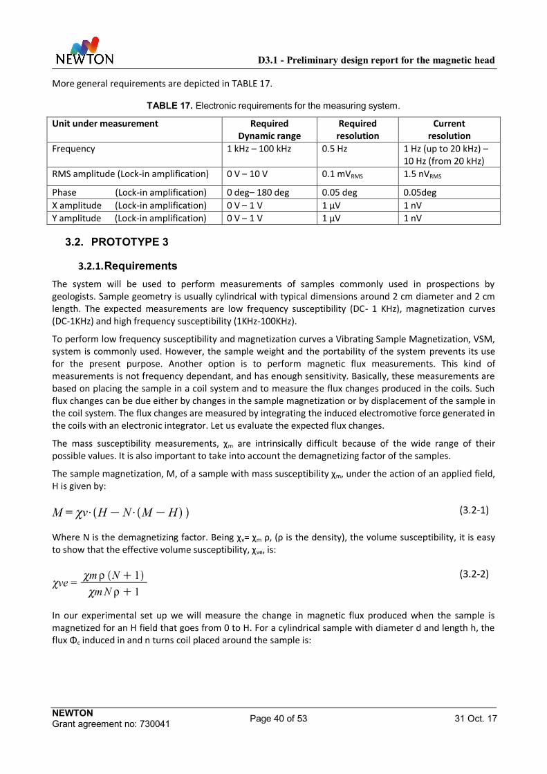
D3.1 - Preliminary design report for the magnetic head
NEWTON Grant agreement no: 730041 Page 40 of 53 31 Oct. 17
More general requirements are depicted in TABLE 17.
TABLE 17. Electronic requirements for the measuring system.
Unit under measurement Required Dynamic range
Required resolution
Current resolution
Frequency 1 kHz – 100 kHz 0.5 Hz 1 Hz (up to 20 kHz) – 10 Hz (from 20 kHz)
RMS amplitude (Lock-in amplification) 0 V – 10 V 0.1 mVRMS 1.5 nVRMS
Phase (Lock-in amplification) 0 deg– 180 deg 0.05 deg 0.05deg X amplitude (Lock-in amplification) 0 V – 1 V 1 µV 1 nV Y amplitude (Lock-in amplification) 0 V – 1 V 1 µV 1 nV
3.2. PROTOTYPE 3
3.2.1. Requirements The system will be used to perform measurements of samples commonly used in prospections by geologists. Sample geometry is usually cylindrical with typical dimensions around 2 cm diameter and 2 cm length. The expected measurements are low frequency susceptibility (DC- 1 KHz), magnetization curves (DC-1KHz) and high frequency susceptibility (1KHz-100KHz).
To perform low frequency susceptibility and magnetization curves a Vibrating Sample Magnetization, VSM, system is commonly used. However, the sample weight and the portability of the system prevents its use for the present purpose. Another option is to perform magnetic flux measurements. This kind of measurements is not frequency dependant, and has enough sensitivity. Basically, these measurements are based on placing the sample in a coil system and to measure the flux changes produced in the coils. Such flux changes can be due either by changes in the sample magnetization or by displacement of the sample in the coil system. The flux changes are measured by integrating the induced electromotive force generated in the coils with an electronic integrator. Let us evaluate the expected flux changes.
The mass susceptibility measurements, χm are intrinsically difficult because of the wide range of their possible values. It is also important to take into account the demagnetizing factor of the samples.
The sample magnetization, M, of a sample with mass susceptibility χm, under the action of an applied field, H is given by:
(3.2-1)
Where N is the demagnetizing factor. Being χv= χm ρ, (ρ is the density), the volume susceptibility, it is easy to show that the effective volume susceptibility, χve, is:
(3.2-2)
In our experimental set up we will measure the change in magnetic flux produced when the sample is magnetized for an H field that goes from 0 to H. For a cylindrical sample with diameter d and length h, the flux Φc induced in and n turns coil placed around the sample is:
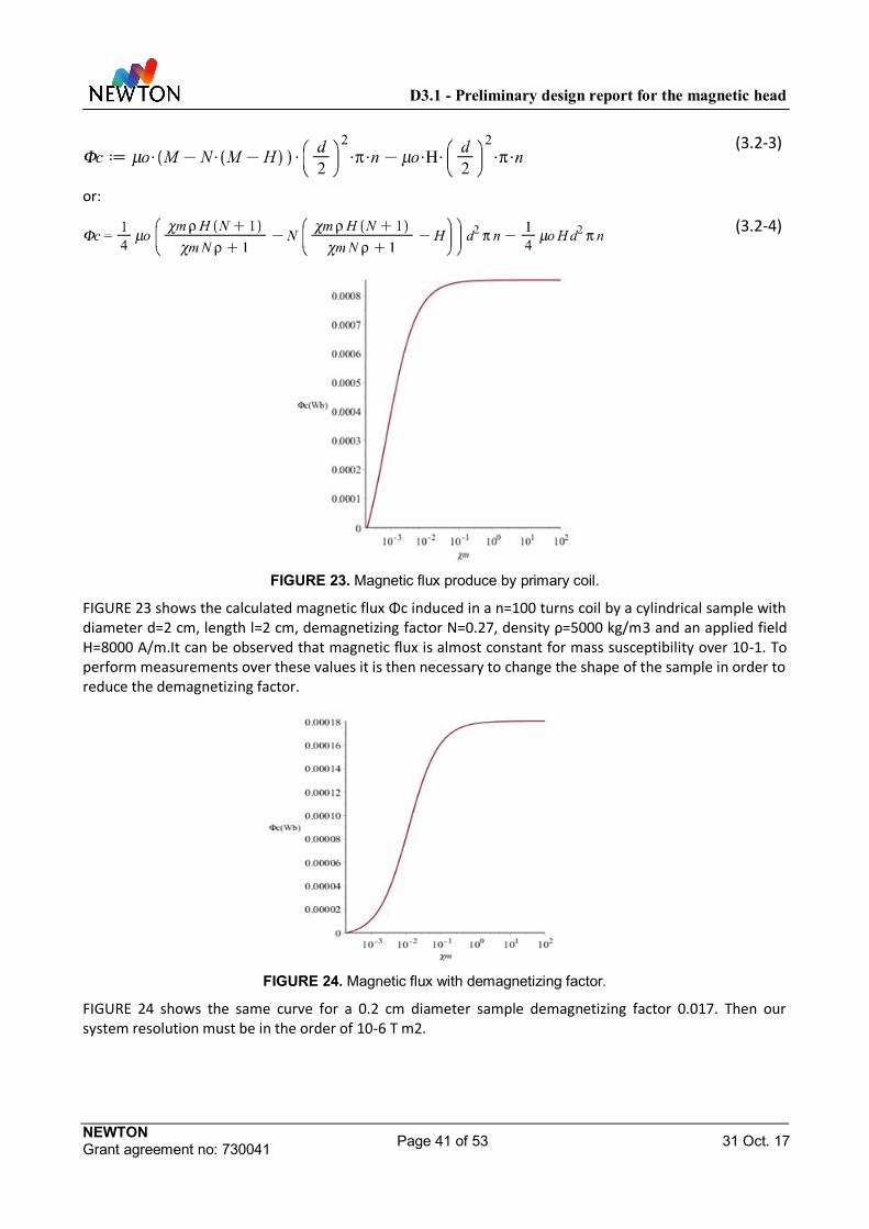
D3.1 - Preliminary design report for the magnetic head
NEWTON Grant agreement no: 730041 Page 41 of 53 31 Oct. 17
(3.2-3)
or:
(3.2-4)
FIGURE 23. Magnetic flux produce by primary coil.
FIGURE 23 shows the calculated magnetic flux Φc induced in a n=100 turns coil by a cylindrical sample with diameter d=2 cm, length l=2 cm, demagnetizing factor N=0.27, density ρ=5000 kg/m3 and an applied field H=8000 A/m.It can be observed that magnetic flux is almost constant for mass susceptibility over 10-1. To perform measurements over these values it is then necessary to change the shape of the sample in order to reduce the demagnetizing factor.
FIGURE 24. Magnetic flux with demagnetizing factor.
FIGURE 24 shows the same curve for a 0.2 cm diameter sample demagnetizing factor 0.017. Then our system resolution must be in the order of 10-6 T m2.

D3.1 - Preliminary design report for the magnetic head
NEWTON Grant agreement no: 730041 Page 42 of 53 31 Oct. 17
The dynamic range of the system must go from 0 up to the maximum expected value.
To evaluate the maximum expected magnetic flux we have calculated the flux induced in a 100 turns coil by cylinder of iron with the size mentioned above
(3.2-5)
3.2.2. Magnetic measuring set-up First device. AC magnetic field measurement system
Measurements must be very accurate and for low susceptibility measurement since the emf induced by the field H can be orders of magnitude greater than the one induced by the sample. To avoid this the part of the induced emf in the secondary coil by H must be compensated. This compensation can be done with a second coil connected in opposition with the first coil and subject to the same field H, then it is necessary a very uniform H to guarantee that the both secondary coils are immersed in the same field. Additionally, both coils must be exactly equal in size, self-inductance and winding, which is almost impossible.
If the field H were not uniform compensation will be obtained displacing adequately the two coils, but we need a uniform field H to magnetize correctly the sample. We have solved the problem with a second pair of coils with less turns placed close to the end coils that produces the field H, this is in the zone were the magnetic field H changes abruptly.
There are three possible measurement modes:
1. The sample placed inside of one central secondary and to change the field H to induce a magnetic flux change in the coils.
2. The sample is displacing alternatively from a coil to the other under a constant field H, in this case the flux change is only due to sample constant magnetization.
3. The sample is displacing alternatively from a coil to the other under an AC field H of constant amplitude, in this case the change in amplitude and phase of the AC induced emf is only due to sample alternating magnetization.
In 1 and 2 method a fluxmeter integrator will be used in 3 it will be used a lock-in amplifier to measure the real and complex part of the susceptibility.
FIGURE 25. Prototype 3 secondary coil mould.
The sample holder diameter is given by the sample diameter and the secondary diameter is given by the sample holder diameter. Besides the sample holder must displace inside secondary without mechanical contact to avoid spurious flux changes. With these conditions the dimensions are shown in FIGURE 25.

D3.1 - Preliminary design report for the magnetic head
NEWTON Grant agreement no: 730041 Page 43 of 53 31 Oct. 17
The head sensitivity is given by the number of turns, n, of the secondary coils. The self-induction depends on n2 so a trade-off between sensitivity and the self-induction needs to be achieved, as we will see later in the electronic design block. For the final system we propose several secondary heads depending on the working frequency. For this preliminary design we have select 500 turns in central coils and 30 turns in the ends coils. The self-induction of this coil is 4 mH and a sample of 2·10-4 mass susceptibility density 5000 under a field of 80 A/m will induce e magnetic flux of 10-6Wb.
FIGURE 26. Magnetic coil for low frequency measurements.
For medium-high frequency measurements a single layer multiturn coil would be used as primary coil. For low frequency measurement, we will use the composed primary coil already presented in the first report D2.1 (FIGURE 26):
1mm diameter wire. 4 layer in coil Resistance 4.7 Ohm Inductance 13.2 mH H field 3680 (A/m)/A The magnetic field uniformity in the central zone 0.011
Second device. DC-ultra low frequency intense magnetic field production system
Magnetic measurements that require low frequencies and strong magnetic fields are commonly carried out using a Vibrating Sample Magnetometer (VSM). This device is based on a mechanical vibrating system, which limits the working frequency, and a big electromagnet to achieve the high field. Typical sample dimensions we may deal with (20 mm diameter, 20 mm length) cannot be measured in this kind of systems because of their relatively high weight (normally incompatible with the vibration system) and the size which exceeds the uniformity area of the magnetic field generated by the electromagnet (see FIGURE 27). For these samples, it would be necessary, at least, 50 mm diameter poles to obtain an adequate uniformity in the zone of the gaps.
One possibility to solve the need of large magnetic poles is to change the poles shape in order to increase the field uniformity. However this modification may reduce the maximum magnetic field.
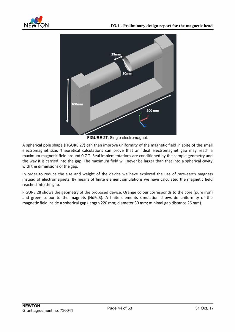
D3.1 - Preliminary design report for the magnetic head
NEWTON Grant agreement no: 730041 Page 44 of 53 31 Oct. 17
FIGURE 27. Single electromagnet.
A spherical pole shape (FIGURE 27) can then improve uniformity of the magnetic field in spite of the small electromagnet size. Theoretical calculations can prove that an ideal electromagnet gap may reach a maximum magnetic field around 0.7 T. Real implementations are conditioned by the sample geometry and the way it is carried into the gap. The maximum field will never be larger than that into a spherical cavity with the dimensions of the gap.
In order to reduce the size and weight of the device we have explored the use of rare-earth magnets instead of electromagnets. By means of finite element simulations we have calculated the magnetic field reached into the gap.
FIGURE 28 shows the geometry of the proposed device. Orange colour corresponds to the core (pure iron) and green colour to the magnets (NdFeB). A finite elements simulation shows de uniformity of the magnetic field inside a spherical gap (length 220 mm; diameter 30 mm; minimal gap distance 26 mm).

D3.1 - Preliminary design report for the magnetic head
NEWTON Grant agreement no: 730041 Page 45 of 53 31 Oct. 17
FIGURE 28. Simulation of magnetic field inside a spherical cavity. (a) Transversal. (b) Longitudinal.
This geometry allows a uniform field of 0.4 T, which is lower than the one inside the complete spherical cavity. However, the uniformity is good enough as the maximum variation of the field is about 1%. Therefore, with this geometry we can achieve a good uniformity and a relatively high magnetic field, with enough room between poles to hold the sample. After those simulations, we should decide either using permanent magnets (in case the magnetic field is high enough to perform geologist measurements) or adding a primary coils system to induce the magnetic field. The area of uniform field does not allow vibrating measurement. This can be solved by using two devices as shown in FIGURE 29.
(a) (b)
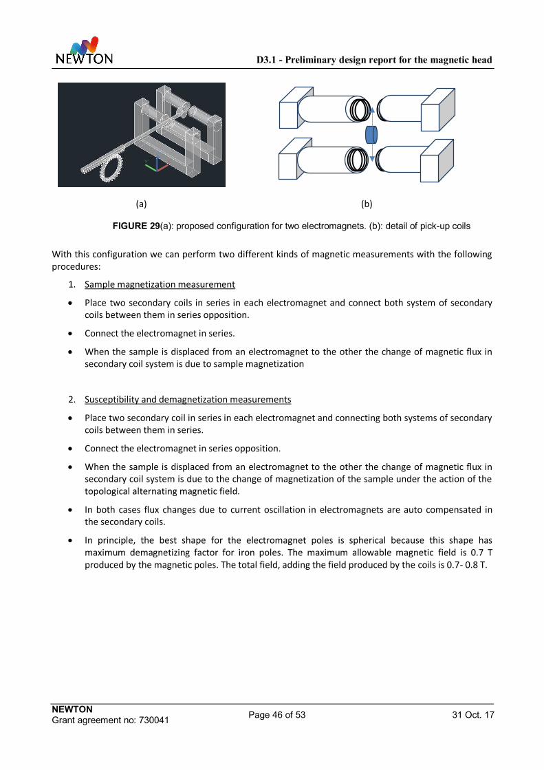
D3.1 - Preliminary design report for the magnetic head
NEWTON Grant agreement no: 730041 Page 46 of 53 31 Oct. 17
(a) (b)
FIGURE 29(a): proposed configuration for two electromagnets. (b): detail of pick-up coils
With this configuration we can perform two different kinds of magnetic measurements with the following procedures:
1. Sample magnetization measurement
Place two secondary coils in series in each electromagnet and connect both system of secondary coils between them in series opposition.
Connect the electromagnet in series.
When the sample is displaced from an electromagnet to the other the change of magnetic flux in secondary coil system is due to sample magnetization
2. Susceptibility and demagnetization measurements
Place two secondary coil in series in each electromagnet and connecting both systems of secondary coils between them in series.
Connect the electromagnet in series opposition.
When the sample is displaced from an electromagnet to the other the change of magnetic flux in secondary coil system is due to the change of magnetization of the sample under the action of the topological alternating magnetic field.
In both cases flux changes due to current oscillation in electromagnets are auto compensated in the secondary coils.
In principle, the best shape for the electromagnet poles is spherical because this shape has maximum demagnetizing factor for iron poles. The maximum allowable magnetic field is 0.7 T produced by the magnetic poles. The total field, adding the field produced by the coils is 0.7- 0.8 T.

D3.1 - Preliminary design report for the magnetic head
NEWTON Grant agreement no: 730041 Page 47 of 53 31 Oct. 17
4. RESULTS AND VALIDATION DATA
4.1. VALIDATION DATA FOR PROTOTYPES 1 AND 2 Despite of the fact that most of the tests performed were focused on the optimization on the design, Ferrite1 configuration has been also measured with reference samples (known content of different magnetic powders). The work done has been partially published in[22], where it is discussed the procedure for the construction, calibration and appropriate use of the susceptometer. Part of the results are reproduced in FIGURE 30.
The calibration was done by means of a set of manufactured samples, constructed with a specific content (wt%) of different magnetic materials. These samples were measured with a VSM ad DC and with a previous version of prototype 3 modified for the calibration of the samples. The measurements with prototype 3 are indicated with the initials of Fixed Susceptomter (FS) in the graphics. The results obtained for the susceptibility were used to tune the results obtained with the Ferrite 1 configuration prototype, indicated by the Portable Susceptometer initials (PS), as they were obtained at very similar frequencies. Due to the nature of the samples source, based on fine powder of the different materials diluted in non-magnetic epoxy formerly hardened, the expected imaginary component at the lowest frequencies was very small and thus, the results could be comparable to the data provide by the VSM.
Once the response of the PS was calibrated with the reference samples manufactured ad hoc of NEWTON instrument calibration, a number of natural samples for different terrestrial scenarios were measured and compared to the results obtained with the FS, VSM and a commercial susceptometer.
The imaginary component could not be calibrated due to the very low imaginary component of the manufactured samples. However, it was made a study of its behavior by means of the study of the power losses of the electrical circuit, and a normalized value for this characteristic was performed, proving the capability of the device to perform this measurement and the capability of provide an absolute value once the susceptometer is fully calibrated.
FIGURE 30. Experimental results for the measurement of the real and normalized imaginary component of the complex magnetic susceptibility with reference samples.

D3.1 - Preliminary design report for the magnetic head
NEWTON Grant agreement no: 730041 Page 48 of 53 31 Oct. 17
4.2. MANUFACTURING AND VALIDATION DATA FOR PROTOTYPE 3 FIGURE 31 shows the secondary set up with the four secondary coils to compensate EMF induced by H. Plastic screws are used to produce a micro displacement inside the primary coils.
FIGURE 31. Secondary coil of prototype 3.
In FIGURE 32 it is shown the mechanical part of the experimental set up the sample holder and the stepper motor displacement system. The sample holder is made of methacrylate for this laboratory set up and the length is the adequate to do not induce magnetic flux changes in secondary coils when it is displaced by the stepper motor. The distance between sample and stepper motor is large enough to avoid spurious inductions.
FIGURE 32. Linear actuator of protyotype 3.

D3.1 - Preliminary design report for the magnetic head
NEWTON Grant agreement no: 730041 Page 49 of 53 31 Oct. 17
In FIGURE 33 it is shown the whole experimental set up including the electronic circuit control board and the connection with the stepper motor.
FIGURE 33. Control board, linear actuator and primary coil of prototype 3.
For high frequency measurement a primary coil with a single layer made of 3mm diameter wire obtaining 300 (A/m)/A. The present design has some heating problems because the high intensity achieved with the resonance. This problem must be solved in the final design.
FIGURE 34. Primary coil for high frequency in prototype 3.
Final measurements require the electronic unit integration. Up to now, we have tested and calibrated the coils for magnetic H production as well as the secondary coils. We have also tested the software and hardware of:
a) The serial communications between PC and the devices.

D3.1 - Preliminary design report for the magnetic head
NEWTON Grant agreement no: 730041 Page 50 of 53 31 Oct. 17
b) ADCs Configuration. Allows the configuration of the microcontrollers AD inputs selecting the
actives and its voltages references. Single measure mode. The selected AD performs a single measure and sends results to
PC. Average measurement mode. The selected AD perform n measurements during a
selected time interval performing an average and sending results to PC. Multiple measurement mode. The selected AD perform m averaged measurements
during a selected time and after each averaged measurement sends the results to PC. c) DACs
Voltage generators for drift and level control Ramps generation and measurement system. It works adequately; it is able to
generate ramps of (213-1) steps performing averaged measurements each k selected steps sending the results to PC.
d) stepper motor control It moves the motor a specified number of steps in a specified time interval andit is also
able to create periodical displacement. It can perform averaged measurements each k selected steps sending the results to
PC.
D3.1 - Preliminary design report for the magnetic head
NEWTON Grant agreement no: 730041 Page 51 of 53 31 Oct. 17
5. SUMMARY AND CONCLUSIONS The designs of the magnetic heads of prototypes 1, 2 and 3 have a significant design.
In all cases the design lines have been introduced with their benefits and disadvantages. In the next period the different options will be analyzed to freeze a design prior to the manufacturing of the prototypes.
The objectives seem to be feasible and it is not expected any delay respect to the proposal calendar.
From the point of view of the team the advance of the project is correct and the interaction between partners has increased significantly.
Furthermore, NEWTON team and LUVMI team have proposed a new testing scenario which will consist in an implementation of prototype 1 in LUVMI rover as a possible representative vehicle for planetary exploration.

D3.1 - Preliminary design report for the magnetic head
NEWTON Grant agreement no: 730041 Page 52 of 53 31 Oct. 17
6. REFERENCES
[1] M. Sanz et al, "Preliminary design report for the electronic control block ", H2020-COMPET-2016 NEWTON - 730041, Report D3.2, October 2017.
[2] C. Lavín et al, "Preliminary design report for power distribution block ", H2020-COMPET-2016 NEWTON - 730041, Report D3.3, October 2017.
[3] M. Díaz-Michelena, R. Kilian, R. Sanz, F. Rios, O. Baeza,“Mars MOURA magnetometer demonstration for high-resolution mapping on terrestrial analogues”. Geosci. Instrum. Methods Data Syst. 5 (2016) 127–142.
[4] R. Singh, R. Lal, U.C. Upreti, D.K. Suri, A.V. Narlikar, V.P.S. Awana, J. Albino Aguiar, Md. Shahabuddin, “Superconductivity in Zn-doped tetragonal laBaCaCu3O7- systems”. Phys. Rev. B 55 (1997) 1216–1222.
[5] C.A.M. Mulder, A.J. van Duyneveldt, J.A. Mydosh, “Susceptibility of the CuMn spin-glass: frequency and field dependences”. Phys. Rev. B 23 (1981) 1384–1396.
[6] E.D. Barco, N. Vernier, J.M. Hernandez, J. Tejada, E.M. Chudnovsky, E. Molins, G. Bellessa, “Quantum coherence in Fe8 molecular nanomagnets”. EPL (Europhys. Lett.) 47 (1999) 722.
[7] P. Marcon, K. Ostanina, “Overview of methods for magnetic susceptibility measurement”. PIERS Proceedings. Malaysia March 27–30 (2012).
[8] S. Foner, “Versatile and sensitive vibrating-Sample magnetometer”. Rev. Sci. Instrum. 30 (1957) 548–557.
[9] M. Pérez, R. Ranchal, I. de Mendizábal Vázquez, P. Cobos, and C. Aroca, “Combined alternating gradient force magnetometer and susceptometer system”. Review of Scientific Instruments 86, 015110 (2015)
[10] G. Asti, M. Solzi, P. Podini, “Phase and frequency control in the vibrating wire magnetic susceptometer”. Sens. Actuators A 81 (2000) 343–345
[11] M. Motta, F. Colauto, R. Zadorosny, T.H. Johansen, R.B. Dinner, M.G. Blamire, G.W. Ataklti, V.V. Moshchalkov, A.V. Silhanek, W.A. Ortiz, “Visualizing the ac magnetic susceptibility of superconducting films via magneto-optical imaging”. Phys. Rev. B 84 (2011) 214529.
[12] S. Li, D. Hurt, M. Toth, B. McElfresh, A. Amann, S. Spagna, “A low background magneto-Optic probe for high, Sens. SQUID Susceptometer”. IEEE Trans. Mag. 50 (11) (2014) 2504704.
[13] Magnetic Susceptibility of volcanic rocks in geothermal areas: application potential in geothermal exploration studies for identification of rocks and zones of hydrothermal alteration. K. Pandarinath, R. Shankar, I.S. Torres-Alvarado, A.K. Warrier.
[14] Magnetic signatures of the orogenic crust of the Patagonian Andes with implica on for planetary explora on. M. Díaz Michelena, R. Kilian.

D3.1 - Preliminary design report for the magnetic head
NEWTON Grant agreement no: 730041 Page 53 of 53 31 Oct. 17
[15] D. Drung, J.-H. Storm, F. Ruede, A. Kirste, M. Regin, T. Schurig, A.M. Repollés, J. Sesé, F. Luis.“Thin-Film Microsusceptometer with integrated nanoloop”. IEEE Trans. Appl. Supercond. 24 (4) (2014) 1600206.
[16] J. Duyn, “MR susceptibility imaging”. J. Magn. Reson. 229 (2013) 198–207.
[17] V.P. Timofeev, C.G. Kim, V.I. Shnyrkov, “Susceptometry application of portable HTS SQUID-Based system”. J. Mag. 3 (3) (1998) 86–88.
[18] C. Lavín et al, "Definition of instrument requirements and architecture. Design guidelines", H2020-COMPET-2016 NEWTON - 730041, Report D2.1, February 2017.
[19] Sanz, R., Fernández, A. B., Dominguez, J. A., Martín, B., and D. Michelena, M., “Gamma Irradiation of Magnetoresistive Sensors for Planetary Exploration”. Sensors, 12, 4447–4465, 2012.
[20] G. Trinkaus, “Magnetic Amplifiers another lost technology”. US Navy 1951.
[21] Lars Austrin, “On Magnetic Amplifiers in Aircraft Applications”. KTH Electrical Engineering. Stockholm 2007.
[22] Marina D. Michelena, J. L. Mesa, M Pérez Jimenez, M. C. Maicas Ramos, P. Cobos Arribas, C. Aroca Hernández-Ros, “A novel induction-based device for the measurement of the complex magnetic susceptibility”. Sensors and Actuators A 263 (2017) 471–479