Embed Size (px)
Citation preview

Ref #5307181 v2.0
New Zealand’s short- and medium-term real exchange rate volatility: drivers and policy
implications
AN2013/03
Willy Chetwin, Tim Ng and Daan Steenkamp
June 2013
Reserve Bank of New Zealand Analytical Note series ISSN 2230-5505
Reserve Bank of New Zealand
PO Box 2498 Wellington
NEW ZEALAND
www.rbnz.govt.nz
The Analytical Note series encompasses a range of types of background papers prepared by Reserve Bank staff. Unless otherwise stated, views expressed are those of the authors, and do
not necessarily represent the views of the Reserve Bank.
Reserve Bank of New Zealand Analytical Note Series 2 _____________________________________________________________
NON-TECHNICAL SUMMARY1 We present some simple measures of realised volatility in New Zealand’s real
exchange rate over the short-term (periods up to one year) and medium term (periods
longer than one year). While New Zealand’s exchange rate volatility at a short run
frequency is not so high as to make it an outlier internationally, exchange rate
volatility has been high compared to the median of the countries considered. Over a
business cycle frequency, New Zealand’s exchange rate has been more volatile than
many of its peers.
We explore reasons for New Zealand’s experience of cycles and short-term noise in
the exchange rate over a period of several decades. There is evidence that the
exchange rate is prone to ‘overshooting’, sometimes persistently, in the sense that its
movements are quite jumpy compared to observed changes in economic
fundamentals. Departures of the exchange rate from its longer-run trend can be quite
large and prolonged.
We argue that the volatility of domestic demand has played an important role in the
volatility of New Zealand’s exchange rate. The exchange rate’s volatility is reasonably
consistent with models describing how an economy moves back towards equilibrium
after being hit by shocks when there are rigidities and frictions in the economy. Policy
seeking to reduce exchange rate volatility can therefore focus on addressing the
domestic sources of economic volatility and the rigidities preventing faster adjustment,
and improving the economy’s resilience to economic and financial volatility.
Monetary policy might be able to affect nominal exchange rate volatility at the margin,
but is unable to deliver persistent reductions in the level of the real exchange rate.
Other policies that affect demand in the economy, such as fiscal policy, are likely to
have a greater and more durable impact. Measures that make the economy more
flexible might also be able to reduce the reactivity of the exchange rate to shocks.
Direct foreign currency intervention measures are unlikely to make a difference to the
cyclical volatility of the real exchange rate, but may be able, at times, to reduce the
effects on short-term fluctuations of simplistic trading rules or poorly formed
expectations.
1 An earlier version of this paper was presented at the Reserve Bank / Treasury Exchange Rate Policy Forum held on 26 March 2013 in Wellington: http://www.rbnz.govt.nz/research/workshops/Mar2013/programme.html

Reserve Bank of New Zealand Analytical Note Series 3 _____________________________________________________________
1. INTRODUCTION The New Zealand dollar exchange rate is widely perceived to be among the more
volatile in its advanced-country peer group.2 Exchange rate volatility is often viewed
as potentially harmful to macroeconomic performance, through adverse effects on
trade or investment, or by encouraging protectionism.3 This paper looks in detail at
the New Zealand experience of exchange rate volatility at different frequencies and
discusses some policy implications.
A currency’s measured volatility relative to others can depend on the particular
measures of volatility used, the horizon or frequency over which movements are
measured, and the approaches taken (if any) to de-trend the data. The policy
implications of volatility similarly depend on the frequency of the volatility. For
example, short-term or high-frequency (e.g. quarterly) volatility may be of little policy
interest if firms can hedge the corresponding exchange rate risk in desired scale and
at a non-deterrent cost (see discussions in Mabin, 2011 and Sanderson, 2009).
Medium-term or business-cycle frequency volatility may be of greater interest to the
extent that hedging markets thin out, or risk management more generally becomes
more expensive, with a horizon lengthening into the business-cycle-frequency range.
Volatility at this frequency is also likely to be more relevant to firms’ longer-term
decisions about investment, employment and market strategy.
Different types of policy actions affect volatility at different frequencies. Some actions
are in the nature of structural policies aiming to improve durably the cyclical and long-
run behaviour of the economy. Others are geared towards shorter-run stabilisation of
the economy when shocks hit or when foreign exchange markets behave in ways
inconsistent with fundamentals.
We focus on exchange rate volatility at the cyclical frequency (periods one or more
years long) and on that at the short-term frequency (one year or shorter). We
distinguish between these frequencies because they differ in the shocks, transmission
mechanisms and market frictions that matter for how volatility affects the economy
and how different policy responses affect outcomes. These differences affect the
assessment of the costs and benefits of potential policy interventions to address
excessive exchange rate volatility.
The rest of the paper proceeds as follows. Section 2 presents summary statistics on
the realised short- and medium-term volatility of the exchange rate in New Zealand
and other countries over a period of several decades, covering a variety of exchange
rate and monetary policy regimes. Sections 3 and 4 discuss volatility at the medium-
term and short-term frequencies respectively, drawing on the New Zealand
2 See e.g. Mabin (2010) and Schmidt-Hebbel (2006). 3 See the general discussion in, for example, Darby, Hughes-Hallett, Ireland and Piscitelli (1999) and Obstfeld and Rogoff (1995).
Reserve Bank of New Zealand Analytical Note Series 4 _____________________________________________________________
macroeconomic experience to shed light on the drivers of this volatility. Section 5
discusses the impact of exchange rate volatility on the economy and Section 6
explores some potential policy interventions to address excessive or damaging
exchange rate volatility. Section 7 concludes.
2. REALISED VOLATILITY: DATA, METHODS AND RESULTS Perhaps the main concern about volatility is that changes in exchange rates can
surprise market participants materially, requiring changes in plans. Earlier plans –
made based on a particular expectation of the future exchange rate – can become
suboptimal when the exchange rate moves unexpectedly.
In the literature, measuring predictability of the exchange rate – and so measuring
volatility “conditional” on predictions – can involve deducing exchange rate
expectations from forward markets (e.g. implied volatility); using empirical models to
predict exchange rate movements; or relating exchange rate volatility to volatility in
the exchange rate’s determinants. Such models can be based on economic theory
that identifies the fundamental determinants of the exchange rate and often treat
exchange rate volatility as being dependent on its own history as well as on the
volatility in other macroeconomic variables.
In this paper, we instead present simple (unconditional) measures of volatility in the
observed exchange rate, referring to these as “experienced” or “realised” volatility.
That is, we do not attempt to measure exchange rate surprises in the way described
above. We illustrate some basic facts about unconditional volatility in New Zealand’s
exchange rate over several decades compared to other countries’ currencies, and we
explore the kinds of factors that have likely been relevant. We leave the analysis of
“conditional” exchange rate volatility for future research.
Experienced or realised volatility is often measured as the typical size of exchange
rate movements over a defined horizon, or as the dispersion of the exchange rate
around its average or trend over a defined window of time (e.g. the standard deviation
of percentage changes or the coefficient of variation).
To measure medium-term or “cyclical” volatility in the level of the exchange rate, we
apply the Bry and Boschan (1971; BB) algorithm, adapted for use on quarterly data.
The BB algorithm requires the researcher to set a number of parameters that affect
the duration of the cycles the algorithm will identify. We follow Harding and Pagan’s
(2002) restrictions on peak-to-trough (PT) and trough-to-peak (TP) durations of
identified cycles to be 2 quarters or longer and full cycles (PTP or TPT) to be 5
quarters or longer. This allows comparability with Schmidt-Hebbel’s (2006) study of
cycles in New Zealand macroeconomic variables, which also used a quarterly cycle
dating algorithm based on the BB procedure (and which we assume used the same

Reserve Bank of New Zealand Analytical Note Series 5 _____________________________________________________________
parameters for minimum phase and cycle durations).4 We then test the sensitivity of
the relative volatility results to changes in these parameters.5
These choices of parameters exclude very short cycles but not very long ones. For all
countries in our sample there is sufficient medium-run variability in the real exchange
rate for a handful of exchange rate cycles to be picked up.6
Our cyclical exchange rate volatility measures are calculated using the BIS’s real
exchange rates based on the BIS’s “narrow” sample of 27 countries.7 This sample of
countries includes both fixed and floating regime currencies and real exchange rates
of countries within currency unions (the euro area). We use a sample period that
starts in January 1964 and ends in September 2012, which encompasses for many
countries (including New Zealand) at least three different exchange rate
arrangements – an internationally-governed system of pegged exchange rates
(Bretton Woods), nationally determined fixed or managed exchange rate regimes
(e.g. New Zealand and Australia immediately prior to floating), and free-floating.8
We measure short-term volatility (sometimes called “noise”) based on central
tendencies of the monthly, quarterly and annual movements in the (log) levels of
exchange rates and relevant macroeconomic variables. Looking at the change in
exchange rates over different frequencies is a similar approach to Mabin’s (2010)
and, relative to the BB algorithm, quite substantially down-weights lower-frequency
volatility (for example, removing a single unit root if present). We add to Mabin’s
(2010) analysis by supplementing the monthly volatility analysis with quarterly and
annual volatility for the calculations of short-term volatility measures, and by
calculating standard deviations as a measure of short-term volatility in addition to the
average absolute change measure she uses.
4 The large international literature on business cycles contains a substantial subset that imposes an upper limit of 32 quarters on the cycle duration, and a lower limit of 6 quarters corresponding to that imposed in Burns and Mitchell’s (1946) seminal study of US business cycles. The upper limit reflects that Burns and Mitchell did not find business cycles longer than 32 quarters (Baxter and King, 1999). The same limits were subsequently and widely used in applied work and in cycle extraction techniques (e.g. Baxter and King, 1999). Cycle results from the BB algorithm applied here could be viewed as comparable with those using explicit bandpass filters such as Baxter and King’s (1999), provided that the variables under consideration do not contain much variance due to low-frequency cycles (i.e. those longer than 33 quarters). 5 The algorithm also features a smoothing step (discussed in Bry and Boschan, 1971 at p. 79) in which the length of a moving average must be chosen. We choose 6 quarters in our base case for this moving average (our main results were not affected by choices of this parameter between 4 and 8 quarters). 6 Mabin (2010) used a “judgemental” approach to identifying medium-term exchange rate cycles, including requiring as a “general rule of thumb” that cycles should be five years or more in duration (i.e. much longer than the 5 quarter minimum cycle length used by Harding and Pagan to replicate NBER business cycle turning points for the US). She did this because she wants to avoid identifying many shorter cycles, which were not the focus of her study. By contrast, shorter cycles at the business cycle frequency are of central importance in our study, because of their importance for monetary policy conduct and for business investment planning. In the case of New Zealand, using a 5-year minimum excludes the substantial 15percent drop and similarly-sized rebound in the exchange rate in 2006-07, for example. Hence, we use the 5-quarter minimum as in Harding and Pagan and Schmidt-Hebbel but also do some sensitivity testing. 7 Effective real exchange rate and macroeconomic data used in this section were sourced from the BIS and Haver, respectively. See Klau and Fung (2006) for documentation of the BIS real exchange rate indices. The real exchange rate short- and medium-term volatilities calculated using these measures (which we choose for cross-country consistency) for New Zealand are similar to those calculated from a real exchange rate for New Zealand calculated from the official TWI and the corresponding domestic and foreign CPIs. 8 See Sullivan (2013) for a history of New Zealand’s exchange rate regimes.

Reserve Bank of New Zealand Analytical Note Series 6 _____________________________________________________________
2.1. RESULTS
2.1.1 MEDIUM-TERM VOLATILITY This section looks at medium term volatility in real exchange rates. The measures we
consider indicate that New Zealand has had both longer and larger upswings and
downswings than most other countries in our sample.
Appendix A shows the identified real exchange rate turning points for each country for
the sample period January 1964 – September 2012, using the base case parameters
stated above.
The number of cycles identified by the algorithm is not very large, making it difficult to
say with much confidence whether there are material differences in cycle
characteristics across our time period, countries or exchange rate regimes. However,
an informal look at the identified turning points for each country suggests little
evidence of systematic differences in cyclical characteristics along such lines.
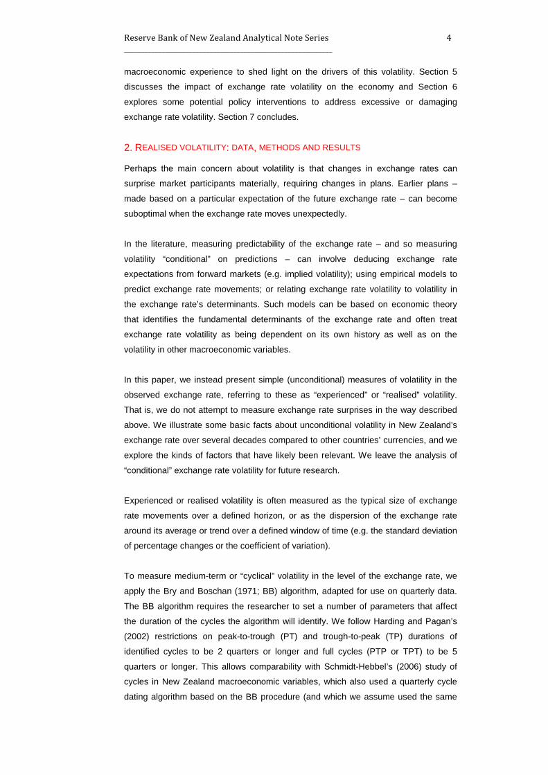
Figures 1 to 3 below show the distribution across countries of the mean and median
lengths of upswings and downswings and the number of cycles. The red dot in each
figure shows the observation for New Zealand; red crosses are ‘outliers’; the red
horizontal line in each box is the median; the top and bottom of each box show the
upper and lower quartile respectively; and the outer pair of horizontal lines – at each
end of the “whiskers” – are the 95th and 5th percentile, respectively.9
One message from these figures is that both real exchange rate upswings and
downswings in New Zealand have tended to be longer than those in the median
country. Reflecting this, over the sample calculated using the BB algorithm with the
parameter settings above, New Zealand (like Canada, Finland, Germany, and the
Netherlands) experienced relatively few complete cycles, eight rather than the median
of 10. Only Japan (7), Greece (6), Spain (5) and Singapore (4) experienced fewer
cycles.
The mean and median appreciation and depreciation in New Zealand’s real exchange
rate over the sample were also larger than the respective means and medians across
the sample countries (median depreciations particularly so). The mean upswing and
downswing magnitude in New Zealand is about 18 to 20 percent relative to the
previous trough or peak. The median country’s was 12 to 14 percent. The countries
that had magnitudes of upswings in the neighbourhood of New Zealand’s are
Australia (17 percent), Spain (18 percent), Singapore (19 percent), Korea (19
percent), Mexico (19 percent), Japan (26 percent) and Taiwan (27 percent). Rankings
for magnitudes of downswings are similar.
9 The full sample is: Australia, Austria, Belgium, Canada, Chinese Taipei, Denmark, Euro area, Finland, France, Germany, Greece, Hong Kong SAR, Ireland, Italy, Japan, Korea, Mexico, Netherlands, New Zealand, Norway, Portugal, Singapore, Spain, Sweden, Switzerland, United Kingdom, United States.

Reserve Bank of New Zealand Analytical Note Series 7 _____________________________________________________________
Figure 1 – Cross-country distributions of mean and median lengths of real exchange rate cycles (quarters), 1964-2011
Observation for New Zealand shown as red dot
Figure 2 – Cross-country distributions of mean and median magnitudes of real exchange rate up- and downswings, 1964-2011
Observation for New Zealand shown as red dot
5
10
15
20
25
30
Qua
rters
Med. length downMean length downMed. length upMean length up
0.05
0.1
0.15
0.2
0.25
%
Med. mag. downMean mag. downMed. mag. upMean mag. up
Reserve Bank of New Zealand Analytical Note Series 8 _____________________________________________________________
Figure 3 – Cross-country distribution of number of real exchange rate cycles, 1964-2011
Observation for New Zealand shown as red dot
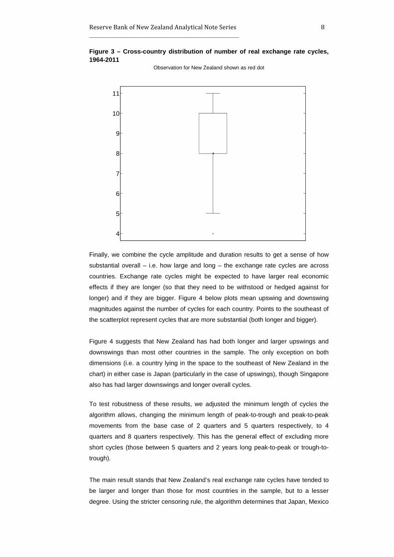
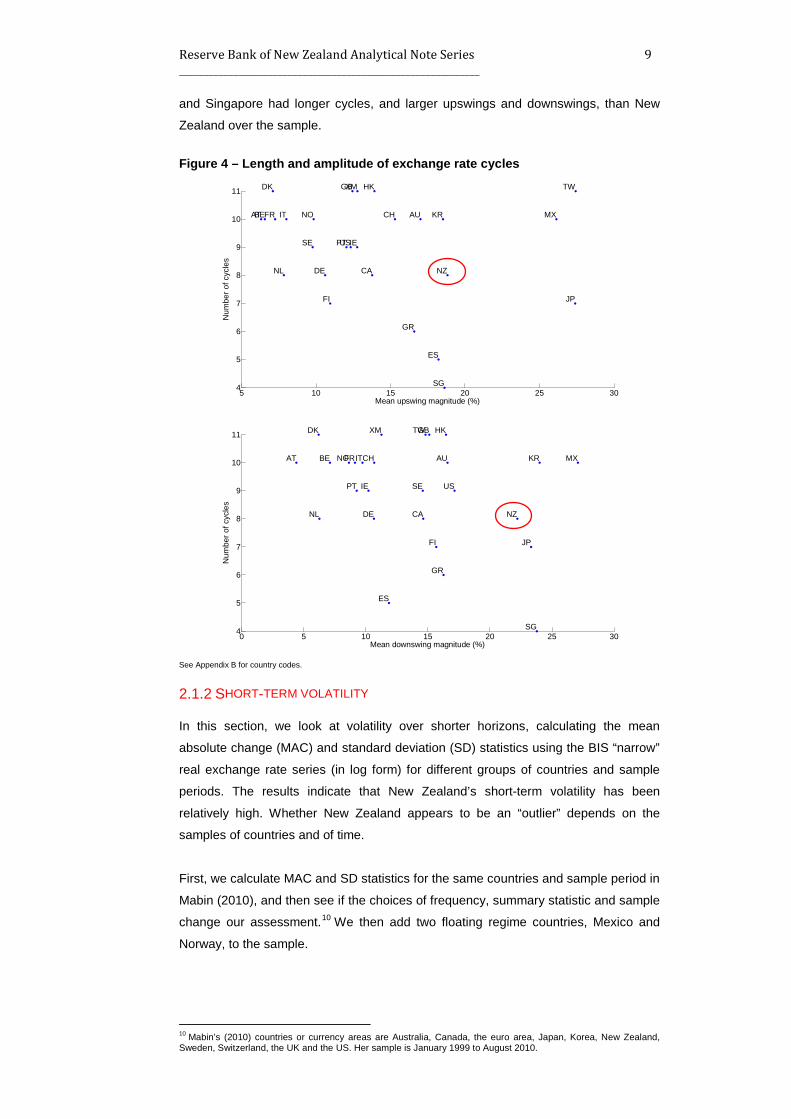
Finally, we combine the cycle amplitude and duration results to get a sense of how
substantial overall – i.e. how large and long – the exchange rate cycles are across
countries. Exchange rate cycles might be expected to have larger real economic
effects if they are longer (so that they need to be withstood or hedged against for
longer) and if they are bigger. Figure 4 below plots mean upswing and downswing
magnitudes against the number of cycles for each country. Points to the southeast of
the scatterplot represent cycles that are more substantial (both longer and bigger).
Figure 4 suggests that New Zealand has had both longer and larger upswings and
downswings than most other countries in the sample. The only exception on both
dimensions (i.e. a country lying in the space to the southeast of New Zealand in the
chart) in either case is Japan (particularly in the case of upswings), though Singapore
also has had larger downswings and longer overall cycles.
To test robustness of these results, we adjusted the minimum length of cycles the
algorithm allows, changing the minimum length of peak-to-trough and peak-to-peak
movements from the base case of 2 quarters and 5 quarters respectively, to 4
quarters and 8 quarters respectively. This has the general effect of excluding more
short cycles (those between 5 quarters and 2 years long peak-to-peak or trough-to-
trough).
The main result stands that New Zealand’s real exchange rate cycles have tended to
be larger and longer than those for most countries in the sample, but to a lesser
degree. Using the stricter censoring rule, the algorithm determines that Japan, Mexico
4
5
6
7
8
9
10
11
Reserve Bank of New Zealand Analytical Note Series 9 _____________________________________________________________
and Singapore had longer cycles, and larger upswings and downswings, than New
Zealand over the sample.
Figure 4 – Length and amplitude of exchange rate cycles
See Appendix B for country codes.
2.1.2 SHORT-TERM VOLATILITY In this section, we look at volatility over shorter horizons, calculating the mean
absolute change (MAC) and standard deviation (SD) statistics using the BIS “narrow”
real exchange rate series (in log form) for different groups of countries and sample
periods. The results indicate that New Zealand’s short-term volatility has been
relatively high. Whether New Zealand appears to be an “outlier” depends on the
samples of countries and of time.
First, we calculate MAC and SD statistics for the same countries and sample period in
Mabin (2010), and then see if the choices of frequency, summary statistic and sample
change our assessment.10 We then add two floating regime countries, Mexico and
Norway, to the sample.
10 Mabin’s (2010) countries or currency areas are Australia, Canada, the euro area, Japan, Korea, New Zealand, Sweden, Switzerland, the UK and the US. Her sample is January 1999 to August 2010.
5 10 15 20 25 304
5
6
7
8
9
10
11
AUATBE
CA
TWDK XM
FI
FR
DE
GR
HK
IE
IT
JP
KR MX
NL NZ
NO
PT
SG
ES
SE
CH
GB
US
Mean upswing magnitude (%)
Num
ber o
f cyc
les
0 5 10 15 20 25 304
5
6
7
8
9
10
11
AUAT BE
CA
TWDK XM
FI
FR
DE
GR
HK
IE
IT
JP
KR MX
NL NZ
NO
PT
SG
ES
SE
CH
GB
US
Mean downswing magnitude (%)
Num
ber o
f cyc
les
Reserve Bank of New Zealand Analytical Note Series 10 _____________________________________________________________
Mabin (2010) reported that for January 1999 to August 2010 New Zealand, Australia
and Japan had the highest short-term exchange rate volatilities, as measured by the
monthly MAC in logs of real exchange rates. Over this period, those countries’ real
effective exchange rates changed month to month by an average 1.8 to 1.9 percent,
just over one standard deviation higher than the country sample mean of 1.4 percent.
The cross-country relativities are about the same for quarterly and annual MACs.
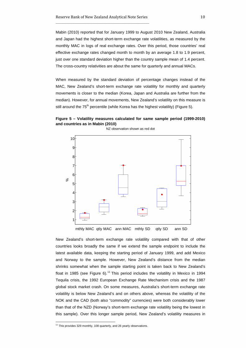
When measured by the standard deviation of percentage changes instead of the
MAC, New Zealand’s short-term exchange rate volatility for monthly and quarterly
movements is closer to the median (Korea, Japan and Australia are further from the
median). However, for annual movements, New Zealand’s volatility on this measure is
still around the 75th percentile (while Korea has the highest volatility) (Figure 5).
Figure 5 – Volatility measures calculated for same sample period (1999-2010) and countries as in Mabin (2010)
NZ observation shown as red dot
New Zealand’s short-term exchange rate volatility compared with that of other
countries looks broadly the same if we extend the sample endpoint to include the
latest available data, keeping the starting period of January 1999, and add Mexico
and Norway to the sample. However, New Zealand’s distance from the median
shrinks somewhat when the sample starting point is taken back to New Zealand’s
float in 1985 (see Figure 6).11 This period includes the volatility in Mexico in 1994
Tequila crisis, the 1992 European Exchange Rate Mechanism crisis and the 1987
global stock market crash. On some measures, Australia’s short-term exchange rate
volatility is below New Zealand’s and on others above, whereas the volatility of the
NOK and the CAD (both also “commodity” currencies) were both considerably lower
than that of the NZD (Norway’s short-term exchange rate volatility being the lowest in
this sample). Over this longer sample period, New Zealand’s volatility measures in
11 This provides 329 monthly, 108 quarterly, and 26 yearly observations.
1
2
3
4
5
6
7
8
9
10
%
ann SDqtly SDmthly SDann MACqtly MACmthly MAC
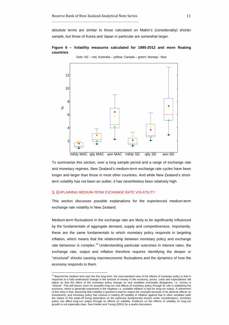
Reserve Bank of New Zealand Analytical Note Series 11 _____________________________________________________________
absolute terms are similar to those calculated on Mabin’s (considerably) shorter
sample, but those of Korea and Japan in particular are somewhat larger.
Figure 6 – Volatility measures calculated for 1985-2012 and more floating countries
Dots: NZ – red; Australia – yellow; Canada – green; Norway - blue
To summarise this section, over a long sample period and a range of exchange rate
and monetary regimes, New Zealand’s medium-term exchange rate cycles have been
longer and larger than those in most other countries. And while New Zealand’s short-
term volatility has not been an outlier, it has nevertheless been relatively high.
3. EXPLAINING MEDIUM-TERM EXCHANGE RATE VOLATILITY This section discusses possible explanations for the experienced medium-term
exchange rate volatility in New Zealand.
Medium-term fluctuations in the exchange rate are likely to be significantly influenced
by the fundamentals of aggregate demand, supply and competitiveness. Importantly,
these are the same fundamentals to which monetary policy responds in targeting
inflation, which means that the relationship between monetary policy and exchange
rate behaviour is complex.12 Understanding particular outcomes in interest rates, the
exchange rate, output and inflation therefore requires identifying the deeper or
“structural” shocks causing macroeconomic fluctuations and the dynamics of how the
economy responds to them.
12 Beyond the medium term and into the long term, the now-standard view of the effects of monetary policy is that in response to a fully-understood change in the amount of money in the economy, prices, costs and expectations will adjust so that the effect of the monetary policy change on real variables eventually disappears, i.e. money is “neutral”. This still leaves room for possible long-run real effects of monetary policy through its role in stabilising the economy, which is generally expressed in the negative i.e. unstable inflation is bad for long-run output. A refinement of this view is that, assuming that volatility in general is bad for output (for example because of its adverse effects on investment), and monetary policy has choices in trading off volatility in inflation against that in other variables (with the nature of this trade-off being dependent on the particular fundamental shocks under consideration), monetary policy can affect long-run output through its effects on volatility. Evidence on the effects of volatility on long-run growth is not especially clear. See Kneller and Young (2001) for a useful discussion.
2
4
6
8
10
12
%
ann SDqtly SDmthly SDann MACqtly MACmthly MAC
Reserve Bank of New Zealand Analytical Note Series 12 _____________________________________________________________
3.1 UNDERSTANDING CYCLICAL EXCHANGE RATE MOVEMENTS A standard view of the exchange rate is that it is an asset price whose value is given
by expected returns available in New Zealand relative to those abroad (see, for
example, Munro, 2004). This principle is captured in the well-known UIP (uncovered
interest parity) relation.
Because expectations are core to the asset price view, expected fundamentals and
not just their current values are relevant to the determination of the exchange rate.
Any of the things affecting the relative economic outlooks of New Zealand and the
global economy, and thus relative expected returns, will affect the currency.13 And
because a change in expectations affects the currency, the exchange rate can move
in advance of things like monetary policy decisions, fiscal policy changes and the
release of data on economic outcomes, to the extent that market participants
continually update their views on these factors.
As we discuss below, empirical literature suggests a significant part of the movement
in the exchange rate can be explained by relative house prices and world commodity
prices (McDonald, 2012 and Munro, 2004), though this says nothing about whether
movements in variables like house prices are driven by underlying activity or some
sort of irrational behaviour.14 Monetary policy, in targeting inflation, also responds to
these shocks since they influence the medium-term behaviour of inflation.
Understanding moves in the exchange rate and interest rates generally requires
understanding the underlying shocks. In general there is a positive co-movement of
interest rates and the exchange rate, reflecting the preponderance of shocks to
aggregate demand.
The macroeconomic balance view of the exchange rate offers a way to interpret
exchange rate developments, by identifying a level of the exchange rate that would be
consistent with definitions of internal balance (for example, output being at potential or
unemployment at its equilibrium rate) and external balance (the current account
balance being consistent with convergence to a sustainable long run net foreign debt
position).
In practice, this identified level is often interpreted as the exchange rate that would
prevail in medium-term equilibrium if the foreign debt position were stable at its
current level as a proportion of the economy. In this view of the equilibrium exchange
rate, prices have had time to adjust and cyclical influences have been removed, but
debt stocks might still be away from and converging to their long run equilibrium
values (see Graham and Steenkamp, 2012). Cyclically adjusted and macro-balance
13 Appendices B and C to an earlier version of this paper provide cross-country views of: how real exchange rate cycle characteristics compare to characteristics in GDP and unemployment cycles; and the volatility of GDP, unemployment, inflation and interest rates. See http://www.rbnz.govt.nz/research/workshops/Mar2013/5200821.pdf 14 Munro also observes that migration flows can help predict the exchange rate, suggesting the reason is that strong migration flows increase housing demand.

Reserve Bank of New Zealand Analytical Note Series 13 _____________________________________________________________
equilibrium exchange rates will therefore differ to the extent that the exchange rate is
driven by non-cyclical factors such as portfolio shifts, such as those that might be
caused by changes in the perceived relative risk of New Zealand assets or of its
external sustainability.
After adjusting for imbalances in the internal economy or external accounts, a macro
balance model tells us how much the exchange rate would have to shift to correct the
imbalance, all else equal. It does not, however, shed light on how the overall
economic adjustment (including that of the exchange rate) might play out, and so is
not predictive in that sense.
3.2 NEW ZEALAND’S RECENT CYCLICAL EXPERIENCE Here we focus specifically on cyclical behaviour of New Zealand’s exchange rate
since the float in 1985 (Figure 7), in the context of how other variables moved as the
business cycle unfolded. Most of the discussion draws on the analyses of past New
Zealand business cycles in Brook, Collins and Smith (1998), Drew and Orr (1999),
Reserve Bank of New Zealand (2000b and 2007), Chetwin (2012) and Chetwin and
Reddell (2012).
Consistent with the view that the predominant real shocks in New Zealand have been
aggregate demand shocks, the longer-lasting of New Zealand’s exchange rate cycles
have coincided with strength in domestic property markets, global demand conditions
and public spending, and in light of all those conditions, expectations of changing
inflation pressure and the monetary policy stance. Large economic shocks stemming
from abroad also at times affected the outlook for New Zealand’s export demand and
commodity prices, leading to some quite sharp movements in the exchange rate.
Figure 7 – The real exchange rate since 1985 (Index 2010 = 100)
Source: Bank for International Settlements
The long economic expansions in the mid-1990s and the mid-2000s coincided with
similarly-long periods of appreciation in the real exchange rate. Similarly, the
recessions and initial periods of recovery leading into the mid-1990s expansion and
60
70
80
90
100
110
120
85 87 89 91 93 95 97 99 01 03 05 07 09 1160
70
80
90
100
110
120Index Index
Narrow
Broad

Reserve Bank of New Zealand Analytical Note Series 14 _____________________________________________________________
following the East Asia Crisis in 1997 saw the exchange rate depreciate from mid-
1988 to mid-1992 and from mid-1997 to the end of 2000.
Those sustained swings in the exchange rate make for an interesting contrast with a
pair of quite sharp down-and-up movements later in the period. The exchange rate
plunged and rebounded in a v-shaped movement between the end of 2005 and
middle of 2007. From there, it dropped again even further, bounced back quickly and
then continued to climb more gradually thereafter.
The sharp drop in 2005 and 2006 appears to have reflected expectations that the
outlook for New Zealand in particular was weakening. Cumulative tightening in
monetary policy was beginning to bear on domestic demand, and real commodity
prices in world terms were easing somewhat from their 2005 levels.
The plunge from late-2007 reflected a major fall in the global growth outlook
coinciding with weakening domestic conditions (and consequent expectations of
easing monetary policy) and reduced international risk appetite. Investors appeared to
believe that the factors that had driven a long period of economic strength were falling
away quickly.
The rebound from the third quarter of 2009 was probably due to an investor emphasis
on strong commodity prices rather than more-general strength. That quite-specific
source of impetus, along with New Zealand’s quite-limited direct exposure to the
causes of the Global Financial Crisis, contributed to New Zealand’s risk-adjusted
outlook being strong relative to some of the major economies in the US and the
European region.
McDonald (2012) provides more formal econometric evidence on a collection of
variables that seems to have mattered for movements in the exchange rate since
June 1986. Among a long list of candidate variables including interest rate
differentials, the growth differential, commodity prices, equity prices, relative house
prices and sales, immigration, and the current account balance, the analysis shows
relative house price inflation, relative house sales volumes and world commodity
prices – all of which can be thought of as indicators of domestic demand pressures
and therefore the risk and return on holding the New Zealand dollar – were on
average, the three most quantitatively important variables explaining movements in
New Zealand’s exchange rate (Figure 8).
The models thus suggest that the exchange rate can be linked to observed
macroeconomic data in a way consistent with the business-cycle view of exchange
rate developments, even though substantial departures from these relationships can
exist over shorter horizons of a few months.

Reserve Bank of New Zealand Analytical Note Series 15 _____________________________________________________________
A significant part of the recent strength in the New Zealand dollar can be attributed to
the near-historic highs of New Zealand’s export commodity prices. 15 Commodity
prices help support spending through income growth and rural land prices, and thus
support the wider economy. Housing market developments have also correlated
strongly with the general business cycle in New Zealand and therefore also the
exchange rate cycle. Current interest rate differentials tend to have low explanatory
power once these other indicators are included in the models.
Figure 8 – Top three statistical drivers of the real exchange rate (deviation from mean)
Source: McDonald (2012).
In line with the evidence in McDonald (2012), large and long rises in house prices in
the mid-1980s, mid-1990s and the mid-2000s had a shape roughly similar to the
climbs in the exchange rate. The same can be said of the housing market downturns
that followed. The periods of house price growth were part of a story of strong
domestic demand, and so the relative growth outlook, inflation outlook and interest
rate outlook of New Zealand.
As well as the global demand cycle, which was a dominant factor driving commodity
prices, a number of large and unpredictable shocks affected New Zealand’s export
demand and commodity prices over the sample. These included the East Asia Crisis
in 1997-98, terrorist attacks of 11th September 2011 in the USA, SARS scare in 2003,
and much later the Global Financial Crisis and subsequent sovereign debt problems.
These events variously kicked off, worsened or prolonged weakness in economic
demand, nervousness about New Zealand’s economic outlook, and reduced risk
appetite, leading in all cases to sharp depreciations.
Some of those shocks, as well as domestic conditions, made for significant net
migrant inflows early in each of the 1990s and 2000s expansions. In the short term,
15 Chen and Rogoff (2003) demonstrate the strong link between commodity prices and the exchange rates of commodity exporters such as Australia, Canada, and New Zealand. Preliminary work at the Reserve Bank suggests that volatility in commodity prices are an important driver of the exchange rate’s volatility in New Zealand.

Reserve Bank of New Zealand Analytical Note Series 16 _____________________________________________________________
strong migration probably added more to demand for consumer durables and for
housing than to supply capacity, contributing to the rise in housing markets.
Domestically, government demand played an important role at times. Late in each of
the 1990s and 2000s expansions when support from abroad began easing,
government spending rose, helping to extend the expansion phases and pressure on
domestic resources (Brook, 2012).
Procyclical financial market conditions contributed to the economic cycle over the
sample period. Rising house prices may have boosted strong private demand and
investment in the rural and residential property sectors. The mid-2000s also featured
a period of compression of credit spreads worldwide amid ample global liquidity and a
search for yield.
All of these factors contributed to substantial macroeconomic cycles in New Zealand.
Indeed, cycles in real per capita GDP and in the unemployment rate have been larger
in New Zealand since 1975 than in a collection of other advanced economies,
according to the results of applying the same BB algorithm as we used in section 2 for
real exchange rates. This observation suggests that the long and large exchange rate
cycles in New Zealand may reflect long and large macroeconomic cycles. However,
scatterplots of the relation between real exchange rate cycle characteristics and GDP
per capita or unemployment rate cycle characteristics shows no particularly strong
relation across countries, suggesting that the relationship is a more complex one.
4. EXPLAINING SHORT-TERM VOLATILITY In this section, we look at the evidence on the degree of short-term noise in New
Zealand exchange rate fluctuations – in other words, the component that is more
difficult to reconcile with movements in medium term fundamentals. As noted in
section 2, in absolute terms the New Zealand dollar (NZD) seems to be noisier at high
frequencies than many other currencies.
4.1 UNDERSTANDING SHORT-TERM VOLATILITY
Short-term exchange rate fluctuations can appear very noisy compared to the path of
the overall economy, and compared to longer run considerations such as relative
purchasing power. Economic modellers often invoke a range of market “frictions” that
slow the adjustment of certain prices to their equilibrium levels in response to shocks,
meaning that quantities and faster-moving prices take the adjustment instead.
Because economists generally view the exchange rate as the fastest moving price in
the economy, such frictions tend to generate increased volatility of the exchange rate
in the face of certain shocks compared to the “frictionless” case.16 For example, in the
16 This could exacerbate the effects of exchange rate movements on the real economy and welfare. Policy aiming to reduce these frictions can help reduce volatility from this source. The horizon where rigidities are most relevant is an empirical question.

Reserve Bank of New Zealand Analytical Note Series 17 _____________________________________________________________
seminal Dornbusch (1976) “overshooting” model, sticky prices in goods markets imply
a jumpier exchange rate in response to shocks because goods prices, by
construction, do not adjust as much as they would under flexible-price assumptions.
Sticky prices are now a standard feature of models of business cycle dynamics (see
for example, Galí and Monacelli, 2005).
Because the exchange rate tends to jump in response to news, and news arrives
daily or more frequently, the jumpiness at high frequencies appears much more
related to very rapid adjustments to expectations among traders than to the slower-
moving measured fundamentals of the economy. Transactions where buyers or
sellers hold open positions for only very short periods, measured on intraday or daily
timescales, tend to represent the majority of daily foreign exchange volumes in New
Zealand currency trading, far in excess of transactions needed to settle or hedge
trade in goods and services (Munro, 2004).17
Over short horizons, high-frequency foreign exchange trading therefore swamps the
influence of the cyclical drivers of currencies. And while such high-frequency activity
increases liquidity, it may also increase volatility by encouraging herding behaviour.18
Foreign currency traders continually update their expectations of relative rates of
return across countries. These, and attitudes to risk, are in turn based on actual and
expected relative interest rate settings and relative growth and inflation.
If the bulk of news is about the future, the present value of expected future
fundamentals may be more volatile than the current values of fundamentals. Changes
in expected relative returns are capitalised immediately into the current level of the
exchange rate. Market sentiment and risk appetite can also affect flows in currency
markets and the exchange rate. While bouts of waning appetite for more risky New
Zealand assets might put downward pressure on the currency, an increase in
uncertainty about the global economy might have the same effect as investors move
funds to “safe haven” assets.
Countries with higher interest rates seem to attract more of the so-called “carry-trade”
investment into domestic currency-denominated bonds. The development of New
Zealand dollar spot and swap foreign exchange markets and an offshore market for
NZD-denominated bonds may also reflect institutional factors such as the credibility of
17 The NZD gets a disproportionate share of global foreign exchange (FX) trade (at 1.6 percent, BIS 2010). Of total NZD transactions, only 36 percent are spot transactions, with the bulk being currency swaps (55 percent), according to the BIS (2010). Offshore activity accounts for around 90 percent of NZD turnover, while total daily FX trade represents over 100 percent of New Zealand’s merchandise trade (McCauley and Scatigna, 2011). While there appears to be a positive relationship between a country’s ratio of FX turnover to trade and its income per capita, New Zealand is still an outlier, with the world’s second highest turnover-to-trade ratio, behind the US. 18 Foreign exchange markets are subject to very short term and simple trading strategies (e.g. chartist or “technical” approaches, including the widespread practice of extrapolative, or “momentum” trading).
Reserve Bank of New Zealand Analytical Note Series 18 _____________________________________________________________
New Zealand’s inflation targeting regime, a general lack of intervention in currency
markets and a relatively strong sovereign credit rating.19
4.2 NEW ZEALAND’S RECENT EXPERIENCE OF SHORT-TERM VOLATILITY The relationship between the exchange rate and its various determinants seems to
change over time. Cassino and Wallis (2010) use a regime-switching model to
examine how financial market participants focus on different individual drivers of the
exchange rate (commodity prices, interest rates or risk appetite) at different points in
time. Risk appetite has, for example, at times replaced changes in relative interest
rates as the key factor driving exchange rate movements at short-term horizons.
However, those risk perceptions could possibly be seen as manifestations of relative
fundamentals. It is also difficult to measure market expectations. This, in turn, makes
it hard to assess the desirability of policy trying to lean against high-frequency
volatility.
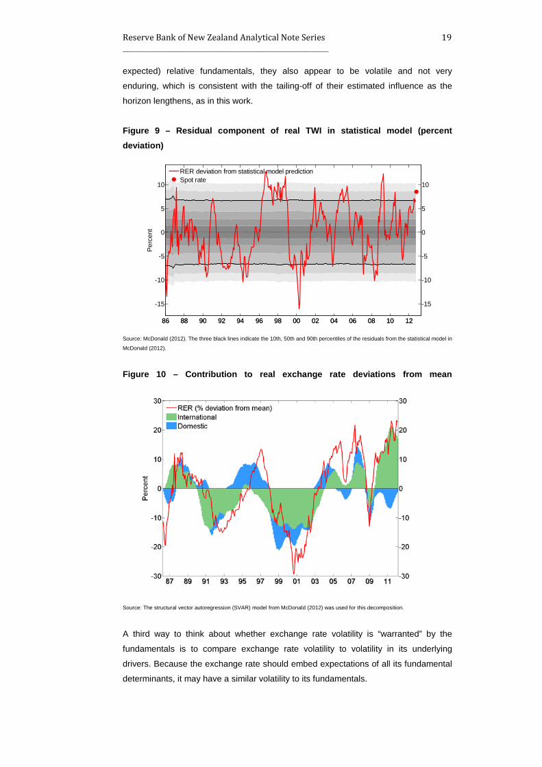
In New Zealand, noise appears at times to be as substantial a component of volatility
as the fundamentals-driven component of the short-term cycle. Over the most recent
past, the portion of the unexplained component of the exchange rate in the McDonald
(2012) indicator model discussed in Section 3 has been unusually large (Figure 9).20
That model suggests that 90 percent of the departures of the exchange rate from the
model’s prediction are up to 7-8 percent in magnitude.
This component unexplained by the indicator model captures un-modelled influences
such as differences in traders’ views of the future (which cannot be observed)
compared to the view implicit in the observed indicators and model structure, any
effects of the simple very short-term trading strategies mentioned above that might be
only tenuously linked to fundamentals, and more general measurement and
specification errors.
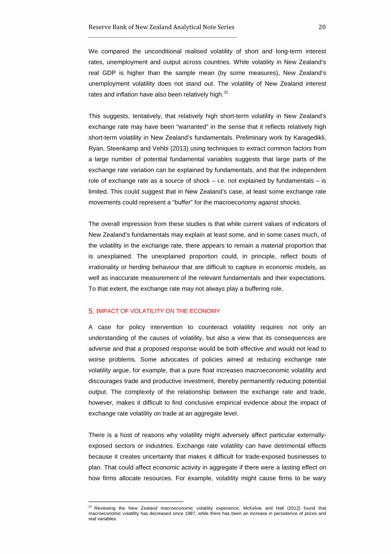
An alternative “structural” approach to explaining exchange rate variance is also
presented in McDonald (2012), which enables the decomposition of exchange rate
movements into international, domestic and residual contributions due to un-modelled
factors such as market sentiment. That model suggests that beyond a horizon of
about one year, the predominant drivers of unexpected exchange rate developments
are international factors (foreign output, prices and interest rates, as well as
commodity prices) (Figure 10). Un-modelled idiosyncratic influences, such as (in this
case) risk-on/risk-off sentiment, however, can explain a high proportion of exchange
rate fluctuations in the very short run. While risk preferences and changes in
perceptions of the global outlook might be expected to relate to current (and
19 It is unclear, though, whether offshore issuance activity contributes to exchange rate volatility. Work by Drage, Munro and Sleeman (2005) suggests that issuance of offshore NZD denominated bonds does not have a large impact on the exchange rate. 20 The indicators in the statistical models are: real commodity prices, terms of trade, real house prices, house sales, relative output gaps, current account, short-term interest rate differentials, long-term interest rate differentials, net migration, relative share market movements.
Reserve Bank of New Zealand Analytical Note Series 19 _____________________________________________________________
expected) relative fundamentals, they also appear to be volatile and not very
enduring, which is consistent with the tailing-off of their estimated influence as the
horizon lengthens, as in this work.
Figure 9 – Residual component of real TWI in statistical model (percent deviation)
Source: McDonald (2012). The three black lines indicate the 10th, 50th and 90th percentiles of the residuals from the statistical model in
McDonald (2012).
Figure 10 – Contribution to real exchange rate deviations from mean
Source: The structural vector autoregression (SVAR) model from McDonald (2012) was used for this decomposition.
A third way to think about whether exchange rate volatility is “warranted” by the
fundamentals is to compare exchange rate volatility to volatility in its underlying
drivers. Because the exchange rate should embed expectations of all its fundamental
determinants, it may have a similar volatility to its fundamentals.
Per
cent
86 88 90 92 94 96 98 00 02 04 06 08 10 12
-15
-10
-5
0
5
10
RER deviation from statistical model predictionSpot rate
86 88 90 92 94 96 98 00 02 04 06 08 10 12
-15
-10
-5
0
5
10
Reserve Bank of New Zealand Analytical Note Series 20 _____________________________________________________________
We compared the unconditional realised volatility of short and long-term interest
rates, unemployment and output across countries. While volatility in New Zealand’s
real GDP is higher than the sample mean (by some measures), New Zealand’s
unemployment volatility does not stand out. The volatility of New Zealand interest
rates and inflation have also been relatively high.21
This suggests, tentatively, that relatively high short-term volatility in New Zealand’s
exchange rate may have been “warranted” in the sense that it reflects relatively high
short-term volatility in New Zealand’s fundamentals. Preliminary work by Karagedikli,
Ryan, Steenkamp and Vehbi (2013) using techniques to extract common factors from
a large number of potential fundamental variables suggests that large parts of the
exchange rate variation can be explained by fundamentals, and that the independent
role of exchange rate as a source of shock – i.e. not explained by fundamentals – is
limited. This could suggest that in New Zealand’s case, at least some exchange rate
movements could represent a “buffer” for the macroeconomy against shocks.
The overall impression from these studies is that while current values of indicators of
New Zealand’s fundamentals may explain at least some, and in some cases much, of
the volatility in the exchange rate, there appears to remain a material proportion that
is unexplained. The unexplained proportion could, in principle, reflect bouts of
irrationality or herding behaviour that are difficult to capture in economic models, as
well as inaccurate measurement of the relevant fundamentals and their expectations.
To that extent, the exchange rate may not always play a buffering role.
5. IMPACT OF VOLATILITY ON THE ECONOMY A case for policy intervention to counteract volatility requires not only an
understanding of the causes of volatility, but also a view that its consequences are
adverse and that a proposed response would be both effective and would not lead to
worse problems. Some advocates of policies aimed at reducing exchange rate
volatility argue, for example, that a pure float increases macroeconomic volatility and
discourages trade and productive investment, thereby permanently reducing potential
output. The complexity of the relationship between the exchange rate and trade,
however, makes it difficult to find conclusive empirical evidence about the impact of
exchange rate volatility on trade at an aggregate level.
There is a host of reasons why volatility might adversely affect particular externally-
exposed sectors or industries. Exchange rate volatility can have detrimental effects
because it creates uncertainty that makes it difficult for trade-exposed businesses to
plan. That could affect economic activity in aggregate if there were a lasting effect on
how firms allocate resources. For example, volatility might cause firms to be wary
21 Reviewing the New Zealand macroeconomic volatility experience, McKelvie and Hall (2012) found that macroeconomic volatility has decreased since 1987, while there has been an increase in persistence of prices and real variables.
Reserve Bank of New Zealand Analytical Note Series 21 _____________________________________________________________
about incurring the ‘sunk’ costs in developing new markets and distribution
infrastructure.
Some exchange rate volatility over the short term may however be a good thing if the
economy is prone to shocks and the exchange rate moves to act as a buffer, for
example, by depreciating when export prices fall or there is external turmoil. Because
domestic prices and wages are often slow to change when foreign prices change, the
exchange rate helps relative prices and wages adjust, helping to reduce the impact of
shocks on the economy’s competitiveness. By contrast, if the exchange rate moves
because of a “portfolio” shock – e.g. a change in risk appetite rather than in
underlying relative demand conditions – the exchange rate may not play that buffering
role.
Over a short horizon, the impact of exchange rate volatility depends on how exports
and imports are priced – e.g. whether the sellers are price setters or takers, and the
currency in which prices are set – and the degree to which firms are able or willing to
adjust their margins. If export prices are set in producers’ domestic currency, an
unexpected appreciation of the exchange rate will tend to be associated with larger
exchange rate pass-through to prices – in particular - import prices would tend to fall
relative to locally produced goods. If export prices are instead set in the currencies of
importers, and prices in goods and services markets were sticky, the New Zealand
dollar price of imports and foreign currency prices of New Zealand exports would be
slow to change when the exchange rate moves. 22 Low (and slow) exchange rate
pass-through in the latter case may have implications for optimal monetary policy (see
Section 6.2.3 and Graham and Smith 2013, forthcoming) as the exchange rate may
not act as an efficient shock-adjustment mechanism and, movements in it can result
in inefficient allocations of resources and consumption.
Volatility may also increase the cost of hedging against currency changes. Long
periods of persistent exchange rate over(under)shooting may also cause supply of
hedging products to decline. By increasing the cost of hedging and business risk,
volatility may impact the hurdle rate for investment in New Zealand. That said, New
Zealand has a relatively sophisticated financial sector offering hedging instruments at
reasonable cost, which allows firms to mitigate some of the effects of exchange rate
fluctuations, at least over shorter horizons.
Low volatility, while it may give more certainty to firms that compete with international
sellers, might attract persistent capital flows (such as carry trade focused on taking
advantage of risk-adjusted returns, with the risk falling when expected volatility in
exchange rates falls). That could contribute to long periods over which the exchange
rate is above or below what underlying economic conditions would otherwise suggest.
Ultimately, such over(under)shooting may be followed by rapid reversion to the mean.
22 Sticky prices can result from various factors, including non-traded costs, mark-up adjustment or nominal price rigidities.

Reserve Bank of New Zealand Analytical Note Series 22 _____________________________________________________________
On the other hand, a degree of exchange rate volatility, like any volatility in the
economy, might promote aggregate productivity if the firms that are able to survive
are the more productive ones, and if it encourages investment that reallocates
resources to the more-productive areas.
To summarise, the real economic effects of the exchange rate are likely to be more
significant at the cyclical frequency than for short term noise in the currency. The
cyclical frequency corresponds most closely to investment planning horizons and
decisions about where to allocate productive resources. It is also probably more
costly – financially and because of uncertainty about the outlook for demand – to
hedge against exchange rate risk over this horizon (Mabin 2011 and Sanderson,
2009). The argument that follows is that cyclical exchange rate movements –
particularly if persistent – could have lasting effects on the composition and
destination of production and composition and source of consumption.
6. POLICY OPTIONS In this section, we look at various policy options that could be considered in the case
where damage to the economy from exchange rate volatility can be shown.
6.1 CHOOSING A DIFFERENT POINT ON THE TRILEMMA Chetwin and Munro (2013) discuss the scope to seek more control over the exchange
rate by fundamentally changing the combination of monetary, exchange rate and
capital account policies – choices in respect of the “trilemma” hypothesis. The
trilemma implies that a country open to capital flows will face a trade-off between
controlling domestic interest rates and controlling the exchange rate; and that the
trade-off can be made less-binding only by reducing openness to capital flows.
Moving away from New Zealand’s current choices of an essentially free float, open
capital markets and monetary policy focused on domestic variables would imply a
change in the nature of economic adjustment to shocks and changing international
conditions. A less-variable exchange rate would put more of the adjustment burden
on domestic prices and output, resulting in greater volatility in output and employment
(see for example Stephens, 2006).
One way for policy to reduce exchange rate variability would be to try to constrain
capital flows, to allow some degree of simultaneous control over both monetary policy
and the exchange rate. This might be pursued through explicit capital or exchange
controls, which target the flow of capital and trading in exchange markets. However,
these come with costs that need to be considered. In particular, they have efficiency
costs and reduce access to offshore funding. There are also questions about their
ability to influence the volume of capital flows for any sustained period (e.g.
Habermeier, Kokenyne and Baba, 2011). Trying to keep the capital account open and
manage both interest and exchange rates would require a substantial stock of foreign

Reserve Bank of New Zealand Analytical Note Series 23 _____________________________________________________________
reserves. That can be costly and expose the Government to considerable exchange
rate risk, and scope to influence the exchange rate through intervention, while
managing interest rates for another objective, is likely to be limited beyond smoothing
shorter-term movements.
Trying to manage both interest rates and the exchange rate involves increased
institutional complexity, because the policy task – managing a number of objectives
that at times can conflict with one another – becomes much more complex. That can
reduce the effectiveness and efficiency of domestic policy institutions and regulation.
It also brings a considerably greater risk of costly policy failure, such as a financial
loss on intervention and sudden sharp shifts in the exchange rate if a peg were
abandoned, or the multiple objectives causing a loss in the credibility of monetary
policy’s commitment to managing inflation which in turn would allow a rise in the level
and volatility of inflation and expectations of inflation.
Measures to restrict capital flows interfere with a country’s access to foreign financing,
raising the cost of capital. Constraining capital flows might also reduce the
opportunities for hedging, by removing from the market natural counterparties for
those wanting to hedge. Further, a fixed exchange rate reduces private incentives to
manage exposure to exchange rate risk through hedging contracts and other
strategies. That means agents will have significant exposure in the event that a build-
up of pressure should lead to a sudden shift in the exchange rate.
6.2 OTHER MEASURES FOR RESPONDING TO MEDIUM-TERM VOLATILITY Because the option of moving away from New Zealand’s current choice of an open
capital account, floating exchange rate and inflation targeting monetary policy would
have such far-reaching structural and institutional ramifications, the policy options we
discuss from here take as given the current choice of a floating regime with open
capital markets.
Within New Zealand’s set of policy choices, we consider policy interventions relating
to volatility attributable to fundamentals as distinct from that relating to noise.
However, a general caveat is that policymakers’ ability to distinguish noise-generated
volatility from that driven by fundamentals is limited, especially in real time. Models
that try to estimate the extent of “excessive” volatility of the exchange rate are
inevitably subject to considerable uncertainty, as suggested by the range of results
from the modelling approaches reviewed in sections 3 and 4. This makes it difficult to
determine whether and exactly when to try to lean against exchange rate volatility,
even if policymakers are generally prepared to lean if circumstances warrant it.
6.2.1 ENHANCING THE FLEXIBILITY OF THE ECONOMY The long and large cycles in New Zealand’s real exchange rate across a number of
quite different nominal exchange rate regimes and several decades (Sullivan, 2013)

Reserve Bank of New Zealand Analytical Note Series 24 _____________________________________________________________
may suggest structural factors play a role. These structural factors can be barriers to
the economy’s flexibility in the face of external shocks, as well as to New Zealand’s
underlying cost competitiveness generally. For example, there might be barriers to the
economy shifting resources to and from trade-exposed sectors when relative prices
change. Monetary policy and exchange rate policy probably have little sway over
these factors, but other policy areas may be able to assist adjustment and promote
smooth adjustment to shocks.
Addressing financial frictions (such as balance sheet constraints on arbitrage, or
incentives to take excessive short-term risk) that amplify the demand effects of
business cycles might dampen the contribution of those frictions to changes in
economic momentum, reducing the work required of monetary policy. Financial
regulatory policy, for example, may help improve risk-management incentives (e.g.
via capital and liquidity requirements) and strengthen arbitrage incentives (e.g. by
promoting deep and complete financial markets).
Enhancing the supply of hedging products may help to reduce the impact of volatility
on the economy. Whether more hedging instruments are ultimately stabilising may
depend, however, on how expectations are formed and how agents learn (see Brock,
Hommes and Wagener, 2009, for example).
In any economy, market expectations may fluctuate between overly optimistic or
pessimistic views of relative asset returns. Policy can help economic adjustment by
being transparent and sufficiently systematic that the market can infer reaction
functions over time.
6.2.2 NON-MONETARY STABILISATION MEASURES Pro-cyclical fiscal policy exacerbates demand pressure and inflation pressure in the
upswing, requiring monetary policy to be more active. This can arise particularly in
sustained economic upswings, when current revenue relieves constraints on
spending and can look increasingly like a structural rise in revenue rather than a
cyclical one. Procyclicality tends to be less of a problem in business cycle
downswings, because a government with a prudent debt position can borrow,
alleviating to some degree the need for a Government to reduce spending. Policy
frameworks that make fiscal spending less procyclical may help reduce the amplitude
of the exchange rate cycle by relieving pressure on monetary policy (see, for
example, Brook, 2012).
Macro-prudential policies seek to enhance financial system resilience in the face of
shocks and cyclical downturns, and to limit the build-up of financial risks in upswings.
Such outcomes can help reduce economic cyclicality in downturns, but any direct
effects of macroprudential measures in the upswing are unlikely to be major. To the
extent that macro-prudential measures can constrain the contribution of the financial
system to domestic cycles, they may reduce the need for monetary policy action, and

Reserve Bank of New Zealand Analytical Note Series 25 _____________________________________________________________
this would affect changes in interest differentials between home and foreign countries,
in turn limiting interest-arbitrage incentives for money to flow into or out of the
domestic currency. That, in turn, could help to relieve pressure on the exchange rate
(see Reserve Bank of New Zealand and Treasury, 2006). In cases where prudential
measures focus on foreign exchange risk on balance sheets, they might also affect
portfolio choice in ways that at the margin reduce exposure to swings in capital flows
and the exchange rate, and so potentially exchange rate volatility in response to
shocks.
Macroprudential tools should be seen as a complement to, not a substitute for,
monetary policy as the primary tool for demand management. Likewise, the effects of
financial sector interventions including macroprudential tools on capital flows and
exchange rate levels are uncertain and could well be limited (Habermeier, Kokenyne
and Baba. 2011). Adjusting such tools to such a degree that they would influence
financial flows or the business cycle in a significant way would probably require quite
major departures from the principle of risk-sensitivity in financial stability regulation,
and thus could cause rather than correct distortions.
6.2.3 MONETARY POLICY MEASURES The review of the medium-term exchange rate volatility experience in sections 2 and
3 emphasised that exchange rate cycles can to a large extent be explained by the
cycles of real aggregate demand and supply and the fundamental domestic and
foreign influences on them. Cycles in the level of aggregate demand relative to supply
capacity imply variations in inflation pressure, so monetary policy also responds to
such cycles. In most countries, shocks to aggregate demand tend to dominate those
to aggregate supply, so interest rates and exchange rates tend to move in the same
direction.
In New Zealand, as in other countries that are credibly committed to price stability as
part of the macroeconomic policy framework, monetary policy has some discretion in
responding to an economic shock. This includes the scope to take exchange rate
considerations into account – within the overall constraint of maintaining price
stability.
Since the passage of the RBNZ Act 1989 required monetary policy conduct to be
governed by a Policy Targets Agreement (PTA), all PTAs have given operational
effect to the principle of flexible inflation targeting, by which the Reserve Bank seeks
to maintain price stability. Flexible inflation targeting as the organising framework for
monetary policy is now mainstream in more than 20 countries worldwide (Roger,
2009), and it is not obvious that there are large potential gains in macroeconomic
performance to be had from variations to the flexible inflation targeting approach.
Despite some differences in inflation targeting frameworks, which appear mostly to be
matters of form rather than substance, a common pattern of low and stable inflation
Reserve Bank of New Zealand Analytical Note Series 26 _____________________________________________________________
has been established in New Zealand and other developed countries since the mid-
1990s.23
In the New Zealand case, the PTA codifies the idea of balancing constraint with
flexibility, so as to stabilise inflation expectations while also allowing room for
monetary policy to exercise some discretion in responding to shocks of different types
as they arise. Successive amendments to the PTA have tended explicitly to allow for
more flexibility (see Reserve Bank of New Zealand, 2000a for a discussion).
Because monetary policy’s response to shocks affects not only the current policy rate
but the future path of interest rates, the monetary policy response is a factor
determining how the exchange rate responds to the shock. The PTA’s current policy
target of “future CPI inflation outcomes between one percent and three percent on
average over the medium term, with a focus on keeping future average inflation near
the two percent target midpoint” provides quantitative guideposts for the extent of
flexibility. PTA clause 3 illuminates further, giving examples of events with temporary
effects to which the monetary policy might be expected to respond using the flexibility
afforded by the policy target. Finally, clause 4(b) requires the Bank to seek to avoid
unnecessary instability in output, interest rates and the exchange rate in its pursuit of
price stability, which is perhaps the most obvious clause by which one might expect
the Bank’s choices of monetary policy response to be coloured by exchange rate
volatility considerations.
In responding to shocks, the Reserve Bank has for some time used the flexibility
afforded by the PTA to take account of the concerns identified in clause 4(b). During
the height of the mid-2000s upswing for example, concern about the high exchange
rate, and a view that cumulative policy tightening and the high exchange rate would
lead demand and inflation pressure to ease further ahead, perhaps led to the OCR
being raised less aggressively than otherwise in the face of high non-tradables
inflation. And in responding to shocks caused by exchange rate movements, the Bank
has generally tried to look through the immediate effects on prices and inflation,
focusing instead on the effect on medium term inflation pressure through changes in
tradables sector incomes and aggregate demand. Again in line with clause 4(b) of the
PTA, this reflects concern that offsetting the first round effects on inflation would
mean a more volatile OCR and possibly output and prices over the medium term (e.g.
Stephens, 2006 and Hampton, Hargreaves and Twaddle, 2006).
More-recent academic literature on monetary policy has started to explore departures
from the law of one price as a reason for monetary policy to lean against exchange
rate movements independently of their effects on inflation. 24 In this view, such
23 Indeed, it is becoming more so, with the Federal Reserve Board of Governors (2012) in the US and the Bank of Japan (2012) recently announcing inflation targets. 24 Such deviations are sometimes viewed as resulting from delayed pass-through of changes in domestic currency import prices to retail prices, although Cavallo, Neiman and Rigobon (2012) suggest that deviations might instead reflect differences in prices when new goods are introduced, rather than reflecting stickiness in prices. Theoretical

Reserve Bank of New Zealand Analytical Note Series 27 _____________________________________________________________
deviations cause costly misallocations of resources and so should be considered as
relevant distortions to be leaned against by monetary policy, in the same way that
distortions caused by price rigidities are now accepted in mainstream monetary theory
as warranting a monetary policy offset.
In most models, the typical gains from adding such exchange rate considerations to
monetary policy objectives are small. Balanced against these considerations are the
risks of reducing the central bank’s policy credibility and hence causing more volatile
inflation expectations, if the approach causes a breach of monetary policy targets.
Financial market participants act on expectations of future policy and economic
conditions, and not just on the current settings. Many market participants would
expect a subsequent policy reversal if settings were inconsistent with inflation
objectives, and so the exchange rate might move little. At the same time, the action
could damage the Reserve Bank’s perceived commitment to price stability and allow
actual inflation to rise. The loss of credibility could raise the perceived risk of investing
in the country and possibly increasing exchange rate volatility.
Trying to limit the amplitude of the exchange rate cycle by using interest rates, without
carefully and transparently reorienting the Reserve Bank’s objectives and underlining
that the overall commitment to price stability remains, risks confusing the public about
those objectives, and causing inflation expectations to become unanchored. Having
said that, the emerging literature exploring distortions in markets that are exposed to
exchange rate fluctuations and their monetary policy implications warrants continued
monitoring.
6.3 MEASURES TO REDUCE SHORT-TERM VOLATILITY AND ITS IMPACT The impacts of exchange rate volatility over short-term horizons might be reduced by
the availability of hedging products and perhaps by prudential policies that ensure
exchange rate risk is prudently managed.
Also, despite the difficulty of identifying and successfully leaning against noise, many
central banks reserve the capacity to intervene (either unilaterally or with the approval
of the government) in foreign exchange markets when it is felt that noise can usefully
be reduced. While foreign currency intervention is the most commonly applied policy
instrument, some countries have also used capital controls.
It is generally accepted that such measures are probably not durably effective if there
are strong fundamental reasons for capital in(out)flows and appreciation
(depreciation) pressure (e.g. Habermeier, Kokenyne and Baba 2011 on capital flow
measures and Adler and Tovar, 2011 on the effectiveness of intervention). Moreover,
all such non-interest rate financial policy measures can be expensive and risky
work indicates that the mechanism of price-setting and the openness of the economy are relevant to the inefficiencies caused by departures from the law of one price.

Reserve Bank of New Zealand Analytical Note Series 28 _____________________________________________________________
(Cassino and Lewis, 2012). 25 At best, intervention may be able to reduce the
amplitude of the currency’s cycle around its long-term average. That is not to say that
intervention might not work when the exchange rate is extremely misaligned or that it
might not limit short-term volatility in the foreign exchange market during a time of
market disorder or thin trading.
The Reserve Bank’s intervention policy stipulates that intervention be limited to
periods where there is market dysfunction or strong evidence of misalignment, as
opposed to trying to engineer level shifts or keep the level of the exchange rate within
certain bounds or trying to use discretionary intervention to smooth movements in the
exchange rate such as in Singapore. There is a high threshold for intervention, with
the requirement that it is consistent with the stance of monetary policy and that it has
a high probability of success.
7. CONCLUSION In this paper, we presented some simple measures of the short-term and cyclical
volatility of the New Zealand real exchange rate. We showed that while New
Zealand’s exchange rate volatility is not so high as to make it an outlier over a short-
run frequency, exchange rate volatility has been high compared to the median of the
countries considered. Over a business cycle frequency, New Zealand’s exchange rate
has been more volatile than many of its peers.
We also explored the reasons for the experienced cycles and short-term noise seen
over several decades in New Zealand. There is evidence that the exchange rate is
prone to ‘overshooting’, sometimes persistently, in the sense that its movements are
quite jumpy compared to observed changes in economic fundamentals. Departures of
the exchange rate from its longer-run trends can be quite large and prolonged.
We argued that the volatility of domestic demand has played an important role in the
volatility of New Zealand’s exchange rate. The volatility is quite consistent with
models of equilibration of the economy when it is hit by shocks and when there are
rigidities or frictions in other parts of the economy. Policy aiming to reduce exchange
rate volatility can therefore focus on addressing the domestic sources of economic
volatility and the rigidities that might prevent the economy responding quickly to
shocks, and improving the economy’s resilience to economic and financial volatility.
Monetary policy might be able to make a difference to nominal exchange rate volatility
at the margin, but it is unable to deliver persistent reductions in the path of the real
exchange rate. Other government policies affecting demand, such as fiscal policy, are
likely to have a greater and more durable impact. Measures to make the economy
25 The extent of foreign trade in the New Zealand dollar also limits the potential impact of intervention and implies that the Bank risks imposing losses on taxpayers. The 2010 triennial survey of foreign exchange market activity by the Bank for International Settlements shows daily New Zealand dollar turnover was about 45 percent of GDP (BIS, 2010).

Reserve Bank of New Zealand Analytical Note Series 29 _____________________________________________________________
more flexible may also be able to reduce the reactivity of the exchange rate to shocks.
Direct foreign currency intervention measures are unlikely to make a difference to the
cyclical volatility of the real exchange rate, but may be able, at times, to reduce the
effects on short-term fluctuations of simplistic trading rules or poorly formed
expectations.
Future work should:
• consider market measures of volatility (such as implied volatility from options
prices) and especially measures of conditional volatility;
• identify different types of shocks and consider their importance in explaining
exchange rate volatility – which would probably require taking a stand on the
temporariness or permanence of the shocks; and
• use volatility measures in structural models to examine the potential effect of
changes in volatility on aggregate and sectoral growth performance.

Reserve Bank of New Zealand Analytical Note Series 30 _____________________________________________________________
REFERENCES Adler, G. and Tovar, C. (2011) “Foreign exchange intervention: a shield against appreciation winds”.
IMF Working Paper Series WP11/65. International Monetary Fund, Washington, DC.
Bank of Japan (2012) “The price stability goal in the medium to long term”. Press release, 14
February.
Baxter, M. and King, R. (1999) “Measuring business cycles: approximate band-pass filters for
economic time series”. The Review of Economics and Statistics 81(4): 575–593.
BIS (2010) “Triennial Central Bank Survey of Foreign Exchange and Derivatives Market Activity in
2010”. Bank for International Settlements, Basel.
Brock, W.A., Hommes, C.H. and Wagener, F.O.O. (2009) “More hedging instruments may destabilize
markets” Journal of Economic Dynamics and Control 33(11): 1912-1928.
Brook, A-M., Collins, S. and Smith, C. (1998) “The 1991-97 business cycle in review”. Reserve Bank
of New Zealand Bulletin 61(4): 269-290.
Brook, A-M. (2012) “Making fiscal policy more stabilising in the next upturn: Challenges and policy
options”. New Zealand Economic Papers, iFirst article: 1-24.
Bry, G. and Boschan, C. (1971) “Cyclical Analysis of Economic Time Series: Selected Procedures
and Computer Programs”. NBER Technical Working Paper No. 20.
Burns, A.F., and Mitchell, W.C. (1946) “Measuring Business Cycles”. National Bureau of Economic
Research, New York, New York.
Cassino, E. and Lewis, M. (2012) “Currency intervention - the profitability of some recent international
experiences”. Reserve Bank of New Zealand Analytical Notes AN2012/03.
Cassino, E. and Wallis, Z. (2010) “The New Zealand dollar through the global financial crisis”.
Reserve Bank of New Zealand Bulletin, 73(3): 20-30.
Cavallo, A., Neiman, B. and Rigobon, R. (2012) "Product Introductions, Currency Unions, and the
Real Exchange Rate," NBER Working Papers Series 18563. National Bureau of Economic
Research, Inc.
Chen, Y. and Rogoff, K. (2003) “Commodity currencies”. Journal of International Economics 60(1):
133-160.
Chetwin, W. (2012) “Business cycle review, 1998-2011”. Reserve Bank of New Zealand Bulletin
75(1): 14-27.
Chetwin, W. and Reddell, M. (2012) “Monetary policy in the last business cycle: some perspectives”.
Reserve Bank of New Zealand Bulletin 75(2): 3-14.
Chetwin, W. and Munro, A. (2013) “Contemporary exchange rate regimes: floating, fixed and hybrid”.
Paper prepared for a joint Reserve Bank-Treasury Forum on the Exchange Rate.
Wellington, 26 March 2013.
Reserve Bank of New Zealand Analytical Note Series 31 _____________________________________________________________
Darby, J., Hughes-Hallett, A., Ireland, J., and Piscitelli, L. (1999) “The impact of exchange rate
uncertainty on the level of investment”. The Economic Journal 109(454): 55–67.
Dornbusch, R. (1976) “Expectations and exchange rate dynamics”. Journal of Political Economy
84(6): 1161-1176.
Drage, D., Munro, A. and Sleeman, C. (2005) “An Update on Eurokiwi and Uridashi Bonds”. Reserve
Bank of New Zealand Bulletin 68(3): 28-38
Drew, A. and Orr, A. (1999) “The Reserve Bank’s role in the recent business cycle: actions and
evolutions”. Reserve Bank of New Zealand Bulletin 62(1): 5-24.
Federal Reserve Board of Governors (2012) “Federal Reserve issues FOMC statement of longer-run
goals and policy strategy”. press release, January 25.
Galí, J. and Monacelli, T. (2005) “Monetary policy and exchange rate volatility in a small open
economy”. The Review of Economic Studies 72(3): 707-734.
Habermeier, K, Kokenyne, A. and Baba, C. (2011) “The effectiveness of capital controls and
prudential policies in managing large inflows”. Staff Discussion Note SDN/11/14.
International Monetary Fund, Washington, DC.
Hampton, T, Hargreaves D. and Twaddle J. (2006) “Other stabilisation objectives within an inflation
targeting regime: Some stochastic simulation experiments”. Reserve Bank of New Zealand
Discussion Paper Series DP2006/04.
Harding, D. & Pagan, A. (2002) “Dissecting the cycle: a methodological investigation,” Journal of
Monetary Economics: 49(2): 365-381.
Graham, J. and Smith, C. (2013), “Optimal monetary policy and the exchange rate,” mimeo.
Graham, J. and Steenkamp, D. (2012), “Extending the Reserve Bank’s macroeconomic balance
model of the exchange rate,” Reserve Bank of New Zealand Analytical Notes series
AN2012/08.
Karagedikli, Ö., Ryan, M., Steenkamp, D and Vehbi, T. (2013) “What happens when the Kiwi flies?
The sectoral effects of exchange rate shocks”. mimeo.
Klau, M. and Fung, S. (2006) “The new BIS effective exchange rate indices”. BIS Quarterly Review,
March.
Kneller, R. and Young, G. (2001) “Business cycle volatility, uncertainty and long-run growth”. The
Manchester School 69(5): 534-552.
Mabin, G. (2010) “New Zealand’s exchange rate cycles: evidence and drivers”. New Zealand
Treasury Working Paper 10/10.
Mabin, G. (2011) “New Zealand’s exchange rate cycles: impacts and policy”. New Zealand Treasury
Working Paper 11/01.
McCauley, R. and Scatigna, M. (2011) “Foreign exchange trading in emerging currencies: more
financial, more offshore”. BIS Quarterly Review March: 67-75.
Reserve Bank of New Zealand Analytical Note Series 32 _____________________________________________________________
McDonald, C. (2012) “Kiwi drivers the New Zealand dollar experience”. Reserve Bank of New Zealand
Analytical Notes AN2012/02.
McKelvie, S. and Hall, V. (2012) “Stylised facts for New Zealand business cycles: A post-1987
perspective”. SEF Working Paper 12/2012 July. Available from
http://hdl.handle.net/10063/2364.
Munro, A. (2004) “What drives the New Zealand dollar?”. Reserve Bank of New Zealand Bulletin
67(2): 21-34.
Obstfeld, M. and Rogoff, K. (1995) “The mirage of fixed exchange rates”. NBER Working Paper
Series 5191.
Reserve Bank of New Zealand (2000a) “The evolution of Policy Targets Agreements”. Independent
review of the operation of monetary policy – Reserve Bank and Non-Executive Directors’
submissions: 18-28. October, Reserve Bank of New Zealand, Wellington.
Reserve Bank of New Zealand (2000b) “Business cycle developments and the role of monetary policy
over the 1990s”. Independent review of the operation of monetary policy – Reserve Bank
and Non-Executive Directors’ submissions: 55-77. October, Reserve Bank of New Zealand,
Wellington.
Reserve Bank of New Zealand (2007) “A review of economic developments and monetary policy
since 2000”. Finance and Expenditure Committee inquiry into the future monetary policy
framework – submission by the Reserve Bank of New Zealand: 36-65. July, Reserve Bank
of New Zealand, Wellington.
Reserve Bank of New Zealand and Treasury (2006) “Supplementary Stabilisation Instruments, Initial
Report to the Governor of the Reserve Bank and Secretary of the Treasury”.
http://www.rbnz.govt.nz/monpol/about/2452274.pdf, February.
Roger, S. (2009) “Inflation targeting at 20: achievements and challenges”. IMF Working Paper Series
WP09/236. International Monetary Fund, Washington, DC.
Sanderson, L. (2009). “Exchange rates and export performance: evidence from micro-data”. Reserve
Bank of New Zealand Bulletin 72(2): 43-52.
Schmidt-Hebbel, K. (2006). “New Zealand’s monetary and exchange-rate policy in international
comparison”. In Testing stabilisation policy limits in a small open economy: 83–144.
Reserve Bank of New Zealand, Wellington.
Stephens, Dominick (2006), “Should Monetary Policy Attempt to Reduce Exchange Rate Volatility in
New Zealand?” Reserve Bank of New Zealand Discussion Paper Series DP2006/05.
Sullivan, R (2013) “New Zealand history of monetary and exchange rate regimes”. Paper prepared for
a joint Reserve Bank-Treasury Forum on the Exchange Rate. Wellington, 26 March 2013.

Reserve Bank of New Zealand Analytical Note Series 33 _____________________________________________________________
APPENDIX A Bry-Boschan turning points in New Zealand’s real exchange rate
Bry-Boschan turning points in real exchange rates by country (log scale; identified peaks and troughs shown in green line; minimum TP/PT=2; minimum PTP/TPT=5. See Appendix B for country codes)
70
80
90
100
110
120
130
64 68 72 76 80 84 88 92 96 00 04 08
Inde
x sa
mpl
e av
erag
e =
100
1964:1 1984:1 2004:14
4.2
4.4
4.6
4.8
5AU
1964:1 1984:1 2004:14.2
4.3
4.4
4.5
4.6
4.7AT
1964:1 1984:1 2004:14.4
4.5
4.6
4.7
4.8
4.9BE
1964:1 1984:1 2004:14.2
4.4
4.6
4.8
5CA
1964:1 1984:1 2004:13
3.5
4
4.5
5
5.5TW
1964:1 1984:1 2004:14.4
4.45
4.5
4.55
4.6
4.65DK
1964:1 1984:1 2004:14.3
4.4
4.5
4.6
4.7
4.8XM
1964:1 1984:1 2004:14.4
4.5
4.6
4.7
4.8
4.9
5FI
1964:1 1984:1 2004:14.5
4.6
4.7
4.8
4.9
5FR

Reserve Bank of New Zealand Analytical Note Series 34 _____________________________________________________________
1964:1 1984:1 2004:14.5
4.6
4.7
4.8
4.9
5DE
1964:1 1984:1 2004:14.2
4.3
4.4
4.5
4.6
4.7GR
1964:1 1984:1 2004:14.4
4.6
4.8
5
5.2HK
1964:1 1984:1 2004:14.3
4.4
4.5
4.6
4.7
4.8IE
1964:1 1984:1 2004:14.3
4.4
4.5
4.6
4.7
4.8IT
1964:1 1984:1 2004:13.8
4
4.2
4.4
4.6
4.8
5JP
1964:1 1984:1 2004:14.2
4.4
4.6
4.8
5
5.2KR
1964:1 1984:1 2004:14
4.2
4.4
4.6
4.8
5MX
1964:1 1984:1 2004:14.4
4.5
4.6
4.7
4.8
4.9NL
1964:1 1984:1 2004:14.2
4.4
4.6
4.8
5NZ
1964:1 1984:1 2004:14.45
4.5
4.55
4.6
4.65
4.7NO
1964:1 1984:1 2004:14
4.2
4.4
4.6
4.8PT
1964:1 1984:1 2004:14.2
4.4
4.6
4.8
5SG
1964:1 1984:1 2004:14.2
4.3
4.4
4.5
4.6
4.7ES
1964:1 1984:1 2004:14.4
4.6
4.8
5
5.2
5.4SE
1964:1 1984:1 2004:14.2
4.4
4.6
4.8
5CH
1964:1 1984:1 2004:14.5
4.6
4.7
4.8
4.9
5
5.1GB
1964:1 1984:1 2004:14.4
4.6
4.8
5
5.2US

Reserve Bank of New Zealand Analytical Note Series 35 _____________________________________________________________
APPENDIX B
Country codes 1 AU Australia
2 AT Austria
3 BE Belgium
4 CA Canada
5 TW Chinese Taipei
6 DK Denmark
7 XM Euro area
8 FI Finland
9 FR France
10 DE Germany
11 GR Greece
12 HK Hong Kong SAR
13 IE Ireland
14 IT Italy
15 JP Japan
16 KR Korea
17 MX Mexico
18 NL Netherlands
19 NZ New Zealand
20 NO Norway
21 PT Portugal
22 SG Singapore
23 ES Spain
24 SE Sweden
25 CH Switzerland
26 GB United Kingdom
27 US United States