New Ultra-Fast Noise Parameter System Opening A … Possibilities in Noise Characterization ... 2009 Agilent Technologies and MAURY ... we can express the noise generators as current

(c) 2009 Agilent Technologies and MAURY

April 2009 Slide 1

New Ultra-Fast Noise

Parameter System...

Opening A New Realm

of Possibilities in Noise

Characterization

David BalloApplication Development EngineerAgilent Technologies

Gary SimpsonChief Technology OfficerMaury Microwave Corporation

2


April 2009 Slide 1

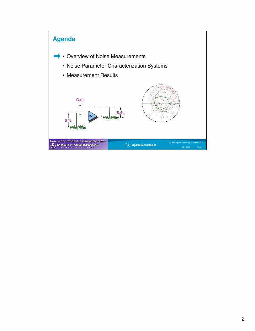
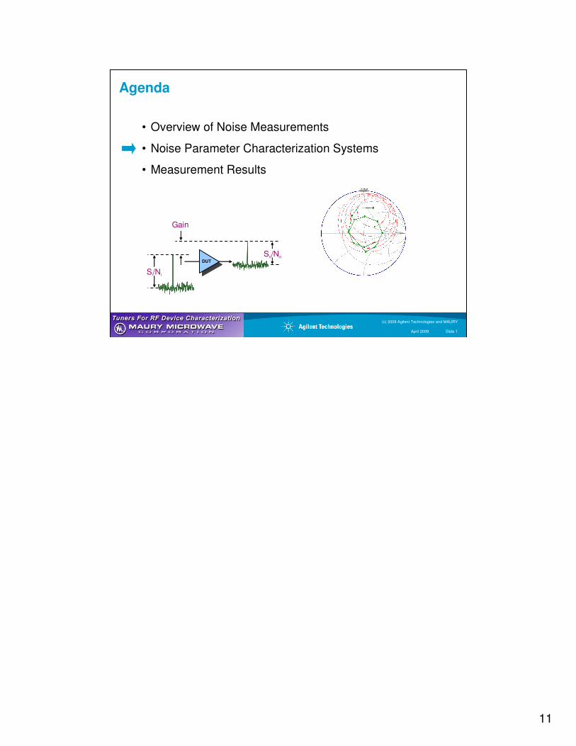
Agenda

• Overview of Noise Measurements

• Noise Parameter Characterization Systems

• Measurement Results

DUT

So/No

Si/Ni

Gain

3


April 2009 Slide 1

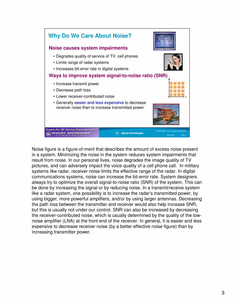
Why Do We Care About Noise?

Noise causes system impairments

• Degrades quality of service of TV, cell phones

• Limits range of radar systems

• Increases bit-error rate in digital systems

Ways to improve system signal-to-noise ratio (SNR)

• Increase transmit power

• Decrease path loss

• Lower receiver-contributed noise

• Generally easier and less expensive to decreasereceiver noise than to increase transmitted power

I

Q

Noise figure is a figure-of-merit that describes the amount of excess noise present

in a system. Minimizing the noise in the system reduces system impairments that result from noise. In our personal lives, noise degrades the image quality of TV

pictures, and can adversely impact the voice quality of a cell phone call. In military

systems like radar, receiver noise limits the effective range of the radar. In digital

communications systems, noise can increase the bit-error rate. System designers

always try to optimize the overall signal-to-noise ratio (SNR) of the system. This can be done by increasing the signal or by reducing noise. In a transmit/receive system

like a radar system, one possibility is to increase the radar’s transmitted power, by

using bigger, more powerful amplifiers, and/or by using larger antennas. Decreasing

the path loss between the transmitter and receiver would also help increase SNR, but this is usually not under our control. SNR can also be increased by decreasing

the receiver-contributed noise, which is usually determined by the quality of the low-

noise amplifier (LNA) at the front end of the receiver. In general, it is easier and less

expensive to decrease receiver noise (by a better effective noise figure) than by

increasing transmitter power.

4


April 2009 Slide 1

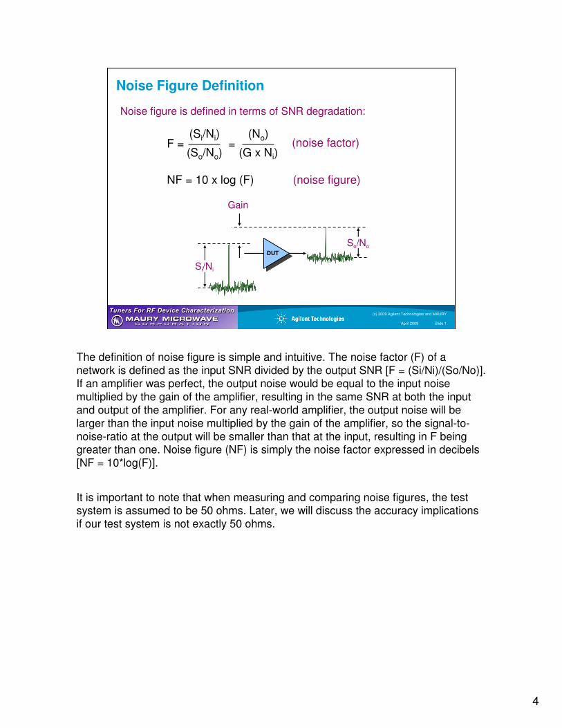
Noise Figure Definition

Noise figure is defined in terms of SNR degradation:

F =(So/No)

(Si/Ni)=

(No)

(G x Ni)(noise factor)

NF = 10 x log (F) (noise figure)

DUT

So/No

Si/Ni

Gain

The definition of noise figure is simple and intuitive. The noise factor (F) of a

network is defined as the input SNR divided by the output SNR [F = (Si/Ni)/(So/No)]. If an amplifier was perfect, the output noise would be equal to the input noise

multiplied by the gain of the amplifier, resulting in the same SNR at both the input

and output of the amplifier. For any real-world amplifier, the output noise will be

larger than the input noise multiplied by the gain of the amplifier, so the signal-to-

noise-ratio at the output will be smaller than that at the input, resulting in F being greater than one. Noise figure (NF) is simply the noise factor expressed in decibels

[NF = 10*log(F)].

It is important to note that when measuring and comparing noise figures, the test system is assumed to be 50 ohms. Later, we will discuss the accuracy implications

if our test system is not exactly 50 ohms.

5


April 2009 Slide 1

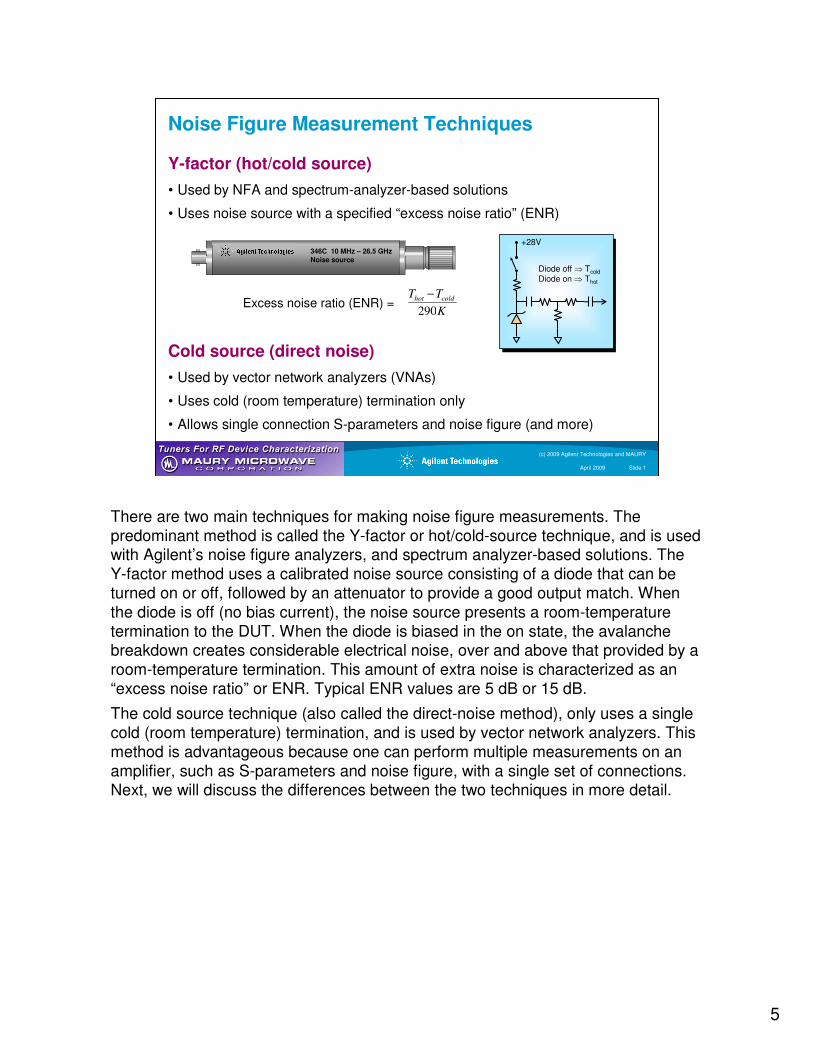
Noise Figure Measurement Techniques

Y-factor (hot/cold source)

• Used by NFA and spectrum-analyzer-based solutions

• Uses noise source with a specified “excess noise ratio” (ENR)

Cold source (direct noise)

• Used by vector network analyzers (VNAs)

• Uses cold (room temperature) termination only

• Allows single connection S-parameters and noise figure (and more)

Excess noise ratio (ENR) =K

TT coldhot

290

−

+28V

Diode off ⇒ Tcold

Diode on ⇒ Thot

Noise source

346C 10 MHz – 26.5 GHz

There are two main techniques for making noise figure measurements. The

predominant method is called the Y-factor or hot/cold-source technique, and is used with Agilent’s noise figure analyzers, and spectrum analyzer-based solutions. The

Y-factor method uses a calibrated noise source consisting of a diode that can be

turned on or off, followed by an attenuator to provide a good output match. When

the diode is off (no bias current), the noise source presents a room-temperature

termination to the DUT. When the diode is biased in the on state, the avalanche breakdown creates considerable electrical noise, over and above that provided by a

room-temperature termination. This amount of extra noise is characterized as an

“excess noise ratio” or ENR. Typical ENR values are 5 dB or 15 dB.

The cold source technique (also called the direct-noise method), only uses a single

cold (room temperature) termination, and is used by vector network analyzers. This

method is advantageous because one can perform multiple measurements on an

amplifier, such as S-parameters and noise figure, with a single set of connections. Next, we will discuss the differences between the two techniques in more detail.

6


April 2009 Slide 1

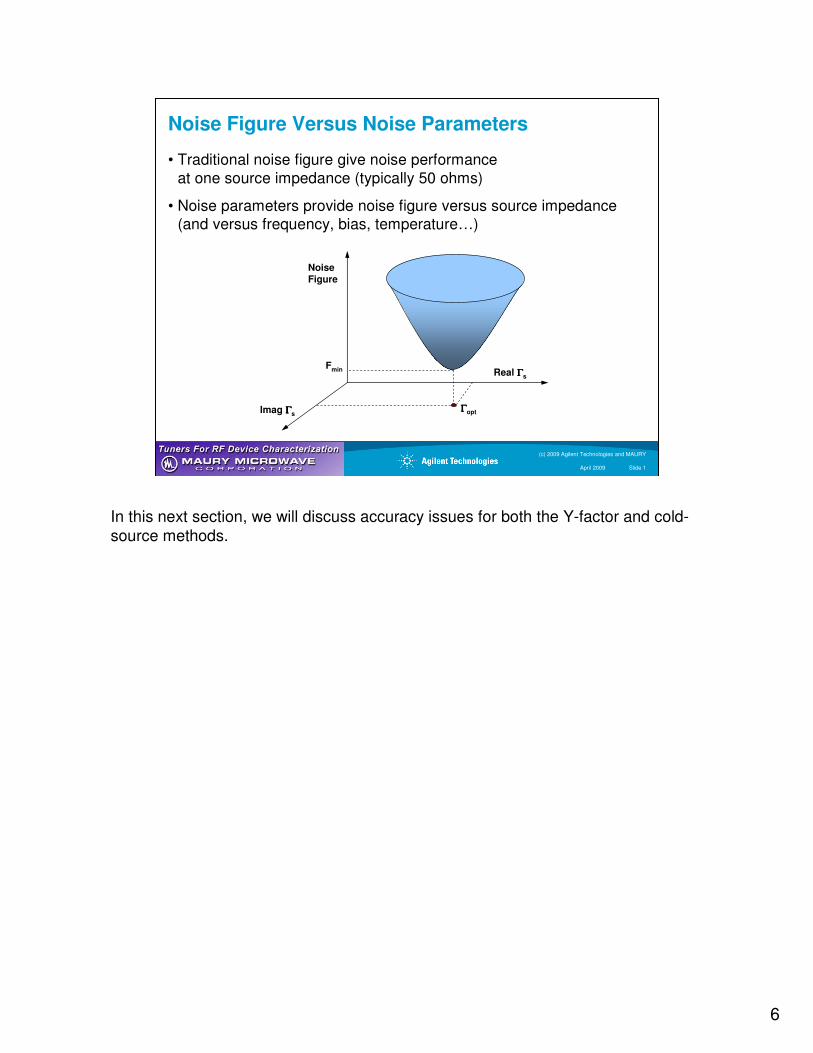
Noise Figure Versus Noise Parameters

• Traditional noise figure give noise performance

at one source impedance (typically 50 ohms)

• Noise parameters provide noise figure versus source impedance(and versus frequency, bias, temperature…)

Real ΓΓΓΓs

Imag ΓΓΓΓs

Fmin

ΓΓΓΓopt

Noise Figure

In this next section, we will discuss accuracy issues for both the Y-factor and cold-

source methods.


April 2009 Slide 1

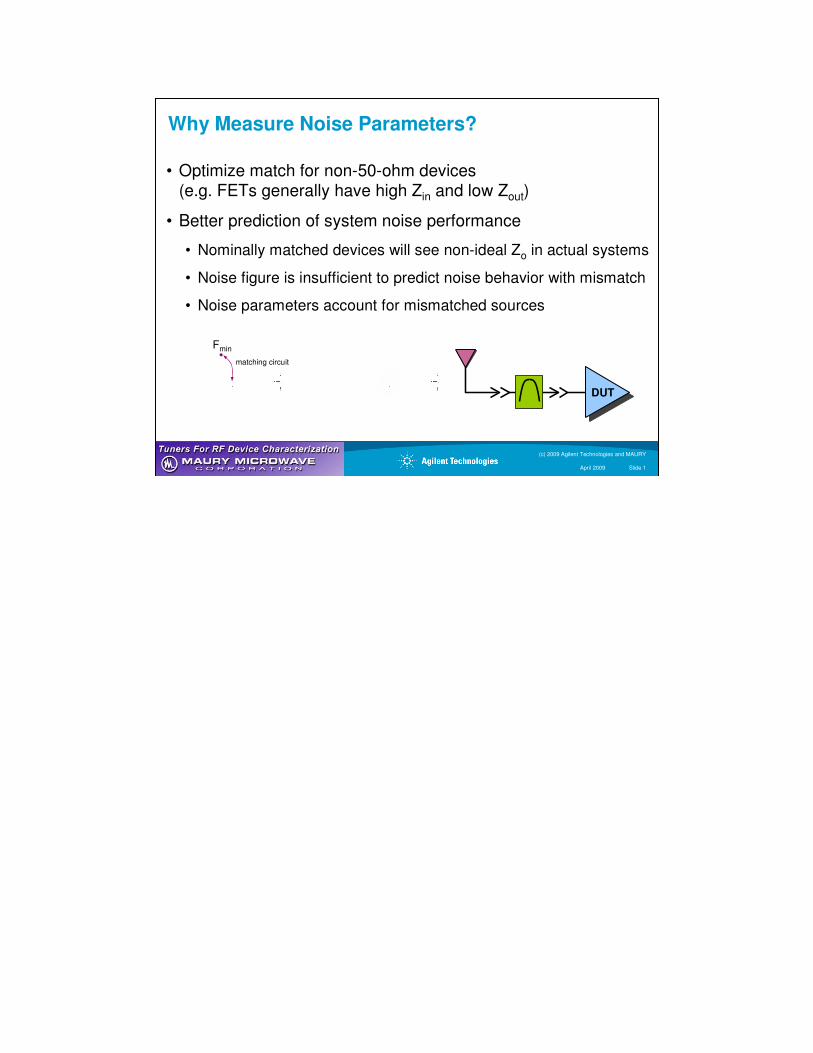
Why Measure Noise Parameters?

• Optimize match for non-50-ohm devices(e.g. FETs generally have high Zin and low Zout)

• Better prediction of system noise performance

• Nominally matched devices will see non-ideal Zo in actual systems

• Noise figure is insufficient to predict noise behavior with mismatch

• Noise parameters account for mismatched sources

DUT

Fmin

matching circuit

8


April 2009 Slide 1

Noise Parameters

( )2

2

min min 2 2

0

4

1 1

Γ − Γ = + − = +

+ Γ − Γ

opt sn ns opt

s opt s

R RF F Y Y F

G Z

Noise figure varies as a function of

source impedance

Noise figure varies as a function of

source impedance

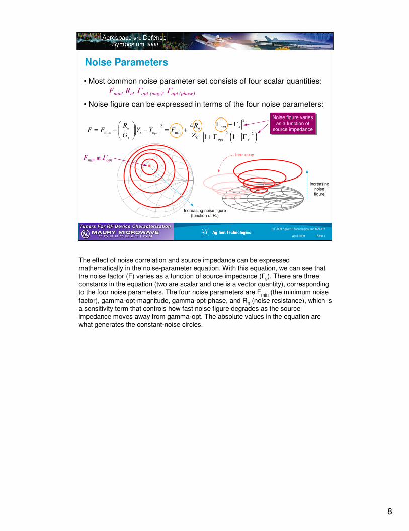
• Most common noise parameter set consists of four scalar quantities:

Fmin, Rn, Γopt (mag), Γopt (phase)

• Noise figure can be expressed in terms of the four noise parameters:

Fmin at Γopt

Increasing noise figure(function of Rn)

Increasing noise figure

frequency

The effect of noise correlation and source impedance can be expressed

mathematically in the noise-parameter equation. With this equation, we can see that

the noise factor (F) varies as a function of source impedance (Γs). There are three

constants in the equation (two are scalar and one is a vector quantity), corresponding

to the four noise parameters. The four noise parameters are Fmin (the minimum noise

factor), gamma-opt-magnitude, gamma-opt-phase, and Rn (noise resistance), which is

a sensitivity term that controls how fast noise figure degrades as the source

impedance moves away from gamma-opt. The absolute values in the equation are

what generates the constant-noise circles.

9


April 2009 Slide 1

Two-Port Noise Models

There are multiple ways to mathematically represent noisy two-port networks:

Z

+ -

e1

+

-

+-

e2

I1

V1

I2

V2

V1 = Z11I1 + Z12I2 + e1

V2 = Z21I1 + Z22I2 + e2

Y+

-

I1

V1

I2

V2

i1 i2

I1 = Y11V1 + Y12V2 + i1

I2 = Y21V1 + Y22V2 + i2

ABCD

+ -e

+

-

I1

V1

I2

V2

iI1 = AV2 + BI2 + i

V1 = CV2 + DI2 + e

Contributes to noise figure

Contributes to gain

Noise sources are generally

independent, with varying degrees of correlation

Noise sources are generally

independent, with varying degrees of correlation

To understand why the noise figure of a device changes versus input match, we must

take a closer look at the noisy two-port model of an amplifier. A noisy two-port network

will have two noise sources, one associated with the input port, and one associated with

the output port. Mathematically, we can express the noise generators as current or

voltage sources, or a mix of both. The bottom representation is popular for noise

analysis, because it separates the noise generators from a perfect gain block, and it is

easier to understand how source match interacts with the two generators. The two noise

sources are generally independent from one another, but typically there is some amount

of correlation between them, depending on the physical and the electrical characteristics

of the amplifier.

10


April 2009 Slide 1

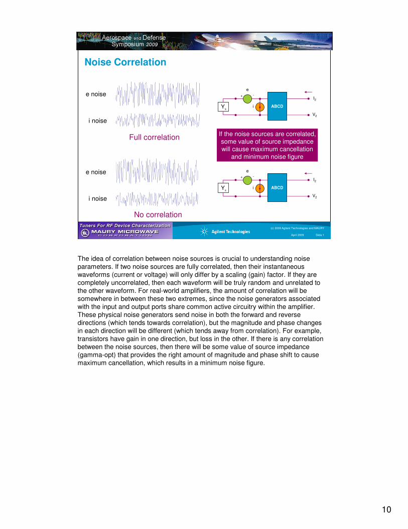
Noise Correlation

e noise

i noise

Full correlation

e noise

i noise

No correlation

If the noise sources are correlated,

some value of source impedance will cause maximum cancellation

and minimum noise figure

ABCD

+ -

e

I2

V2

iYs

ABCD

+ -

e

I2

V2

iYs

The idea of correlation between noise sources is crucial to understanding noise

parameters. If two noise sources are fully correlated, then their instantaneous

waveforms (current or voltage) will only differ by a scaling (gain) factor. If they are

completely uncorrelated, then each waveform will be truly random and unrelated to

the other waveform. For real-world amplifiers, the amount of correlation will be

somewhere in between these two extremes, since the noise generators associated

with the input and output ports share common active circuitry within the amplifier.

These physical noise generators send noise in both the forward and reverse

directions (which tends towards correlation), but the magnitude and phase changes

in each direction will be different (which tends away from correlation). For example,

transistors have gain in one direction, but loss in the other. If there is any correlation

between the noise sources, then there will be some value of source impedance

(gamma-opt) that provides the right amount of magnitude and phase shift to cause

maximum cancellation, which results in a minimum noise figure.

11


April 2009 Slide 1

Agenda




DUT

So/No

Si/Ni

Gain


April 2009 Slide 1

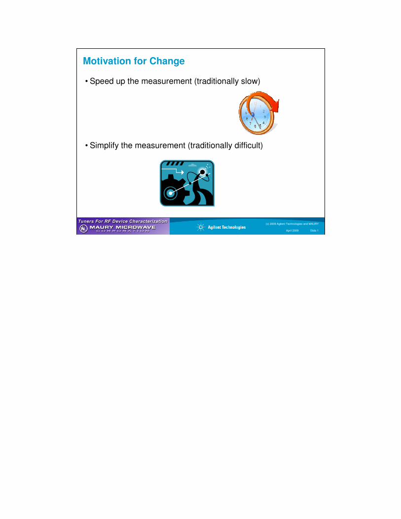
Motivation for Change

• Speed up the measurement (traditionally slow)

• Simplify the measurement (traditionally difficult)


April 2009 Slide 1

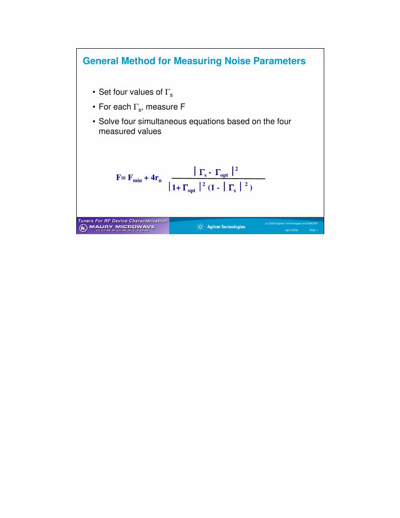
General Method for Measuring Noise Parameters

F= Fmin + 4rn

ΓΓΓΓs - ΓΓΓΓopt 2

1+ ΓΓΓΓopt 2 (1 - ΓΓΓΓs 2

)

• Set four values of Γs

• For each Γs, measure F

• Solve four simultaneous equations based on the four

measured values


April 2009 Slide 1

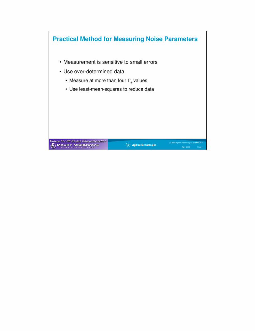
Practical Method for Measuring Noise Parameters

• Measurement is sensitive to small errors

• Use over-determined data

• Measure at more than four Γs values

• Use least-mean-squares to reduce data


April 2009 Slide 1

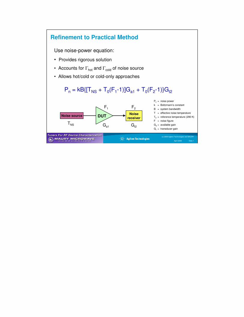
Refinement to Practical Method

Use noise-power equation:

• Provides rigorous solution

• Accounts for Γhot and Γcold of noise source

• Allows hot/cold or cold-only approaches

Pn = kB{[TNS + T0(F1-1)]Ga1 + T0(F2-1)}Gt2

Noise sourceNoise

receiverDUT

TNS Ga1 Gt2

F1 F2

Pn = noise power

k = Boltzmann’s constant

B = system bandwidth

T = effective noise temperature

T0 = reference temperature (290 K)

F = noise figure

Ga = available gain

Gt = transducer gain


April 2009 Slide 1

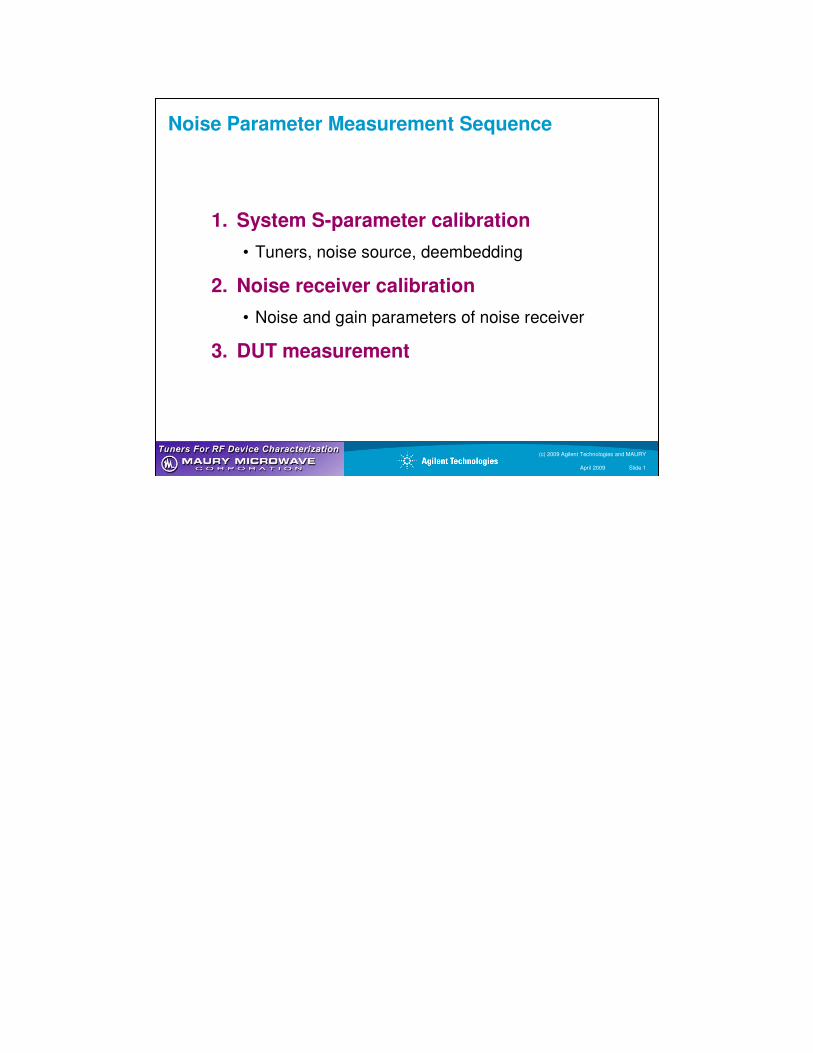
Noise Parameter Measurement Sequence

1. System S-parameter calibration

• Tuners, noise source, deembedding

2. Noise receiver calibration

• Noise and gain parameters of noise receiver

3. DUT measurement


April 2009 Slide 1

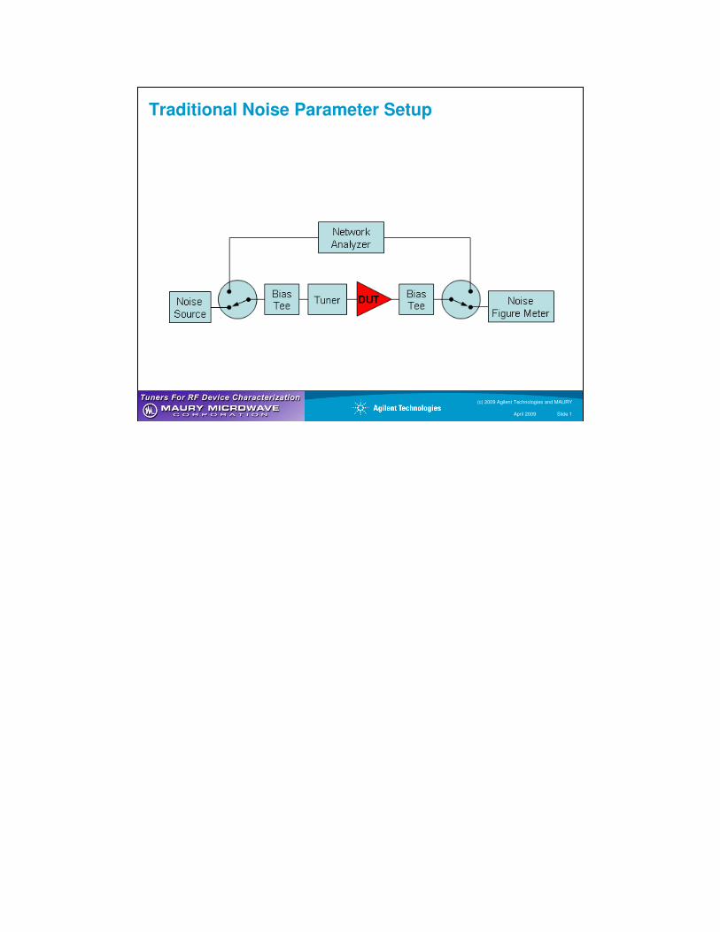
Traditional Noise Parameter Setup


April 2009 Slide 1

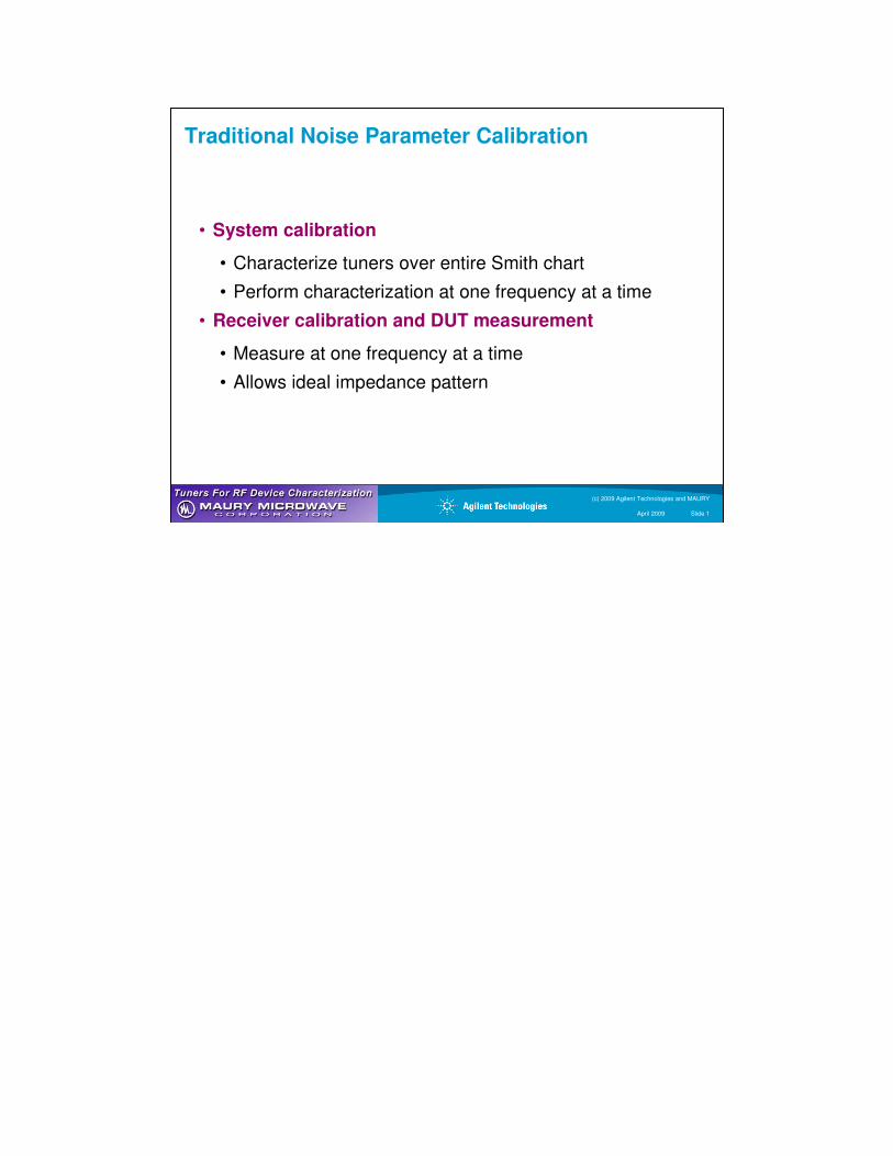
Traditional Noise Parameter Calibration

• System calibration

• Characterize tuners over entire Smith chart

• Perform characterization at one frequency at a time

• Receiver calibration and DUT measurement

• Measure at one frequency at a time

• Allows ideal impedance pattern


April 2009 Slide 1

Limitations of Traditional Method

• Time-consuming procedure

• Tuner probe is moved many, many times during calibration and measurements

• More likely to encounter errors due to drift

• System calibrations

• Used for a long period to save test time

• Calibrating parts separately increases errors


April 2009 Slide 1

History

Heavy objects are hard to move


April 2009 Slide 1

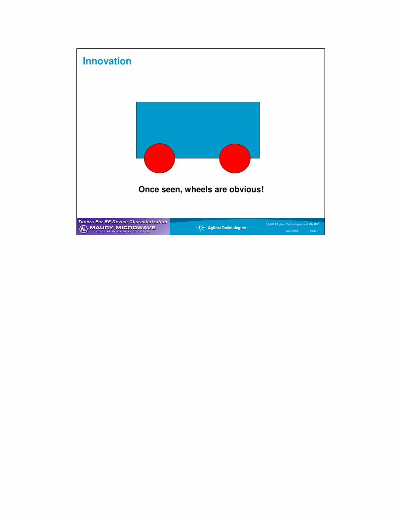
Innovation

Once seen, wheels are obvious!


April 2009 Slide 1

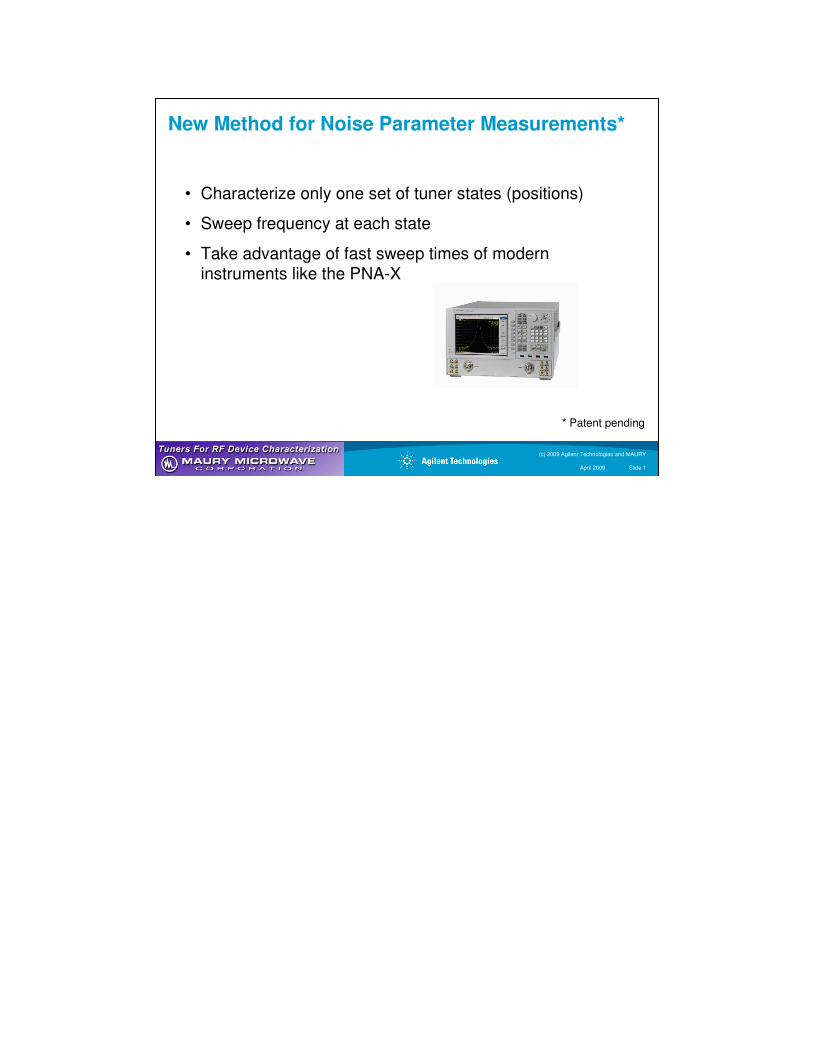
New Method for Noise Parameter Measurements*

• Characterize only one set of tuner states (positions)

• Sweep frequency at each state

• Take advantage of fast sweep times of modern

instruments like the PNA-X

* Patent pending


April 2009 Slide 1

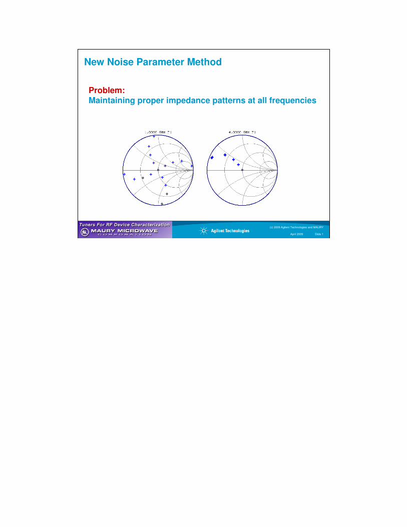
Problem:Maintaining proper impedance patterns at all frequencies

New Noise Parameter Method


April 2009 Slide 1

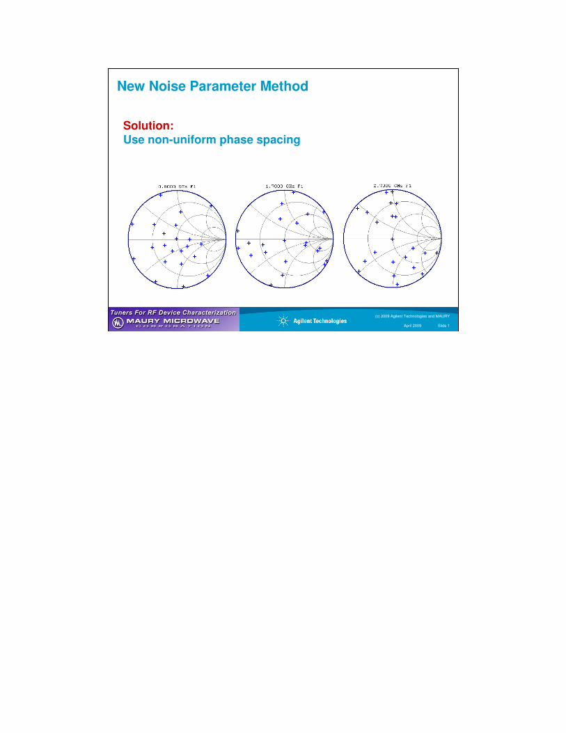
New Noise Parameter Method

Solution:Use non-uniform phase spacing

25


April 2009 Slide 1

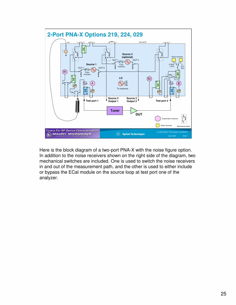
2-Port PNA-X Options 219, 224, 029

DUT

Test port 1

R1

Test port 2

R2

A B

Source 2 Output 1

Source 2 Output 2

rear panel+28V

Noise receivers

10 MHz -

3 GHz

3 -

26.5

GHz

Source 1

OUT 1 OUT 2

Pulse

modulator

Source 2 (optional)

OUT 1 OUT 2

Pulse

modulator

S-parameter receivers

Mechanical switchNoise receivers

J9J10J11 J8 J7 J2 J1

+-

Tuner

To receivers

LO

Here is the block diagram of a two-port PNA-X with the noise figure option.

In addition to the noise receivers shown on the right side of the diagram, two

mechanical switches are included. One is used to switch the noise receivers in and out of the measurement path, and the other is used to either include

or bypass the ECal module on the source loop at test port one of the

analyzer.


April 2009 Slide 1

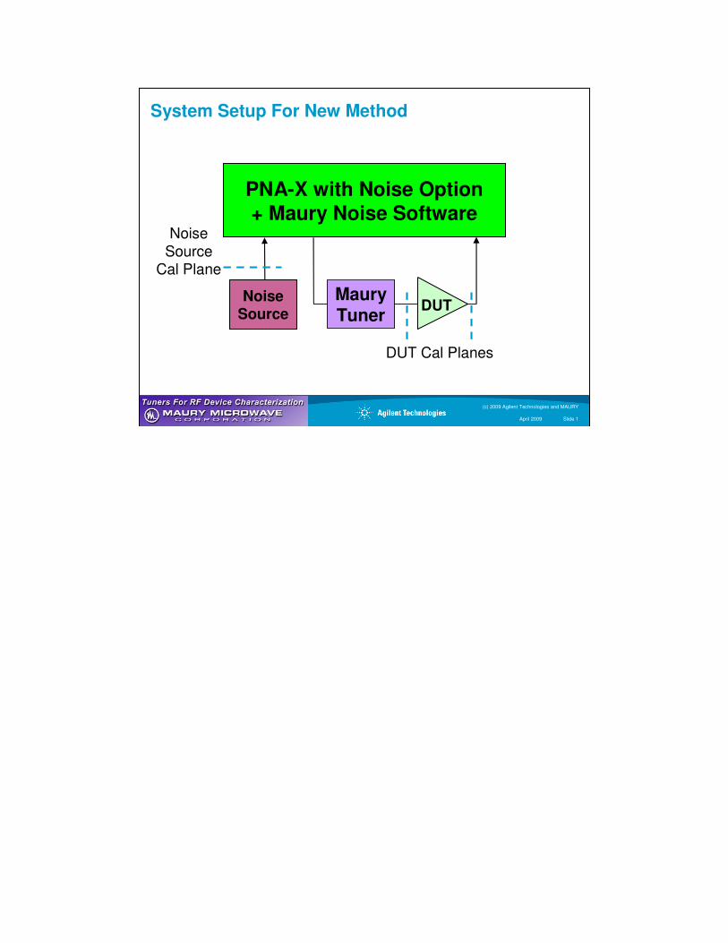
System Setup For New Method

NoiseSource

PNA-X with Noise Option+ Maury Noise Software

MauryTuner

DUT

DUT Cal Planes

Noise

Source Cal Plane


April 2009 Slide 1

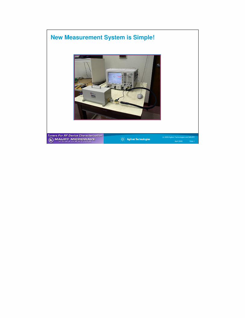
New Measurement System is Simple!


April 2009 Slide 1

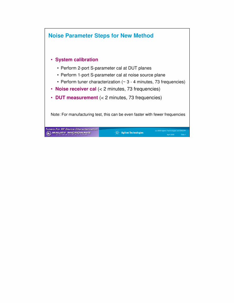
Noise Parameter Steps for New Method

• System calibration

• Perform 2-port S-parameter cal at DUT planes

• Perform 1-port S-parameter cal at noise source plane

• Perform tuner characterization (~ 3 - 4 minutes, 73 frequencies)

• Noise receiver cal (< 2 minutes, 73 frequencies)

• DUT measurement (< 2 minutes, 73 frequencies)

Note: For manufacturing test, this can be even faster with fewer frequencies


April 2009 Slide 1

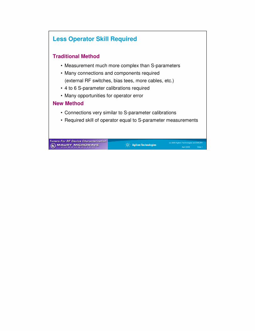
Less Operator Skill Required

Traditional Method

• Measurement much more complex than S-parameters

• Many connections and components required

(external RF switches, bias tees, more cables, etc.)

• 4 to 6 S-parameter calibrations required

• Many opportunities for operator error

New Method

• Connections very similar to S-parameter calibrations

• Required skill of operator equal to S-parameter measurements

30


April 2009 Slide 1

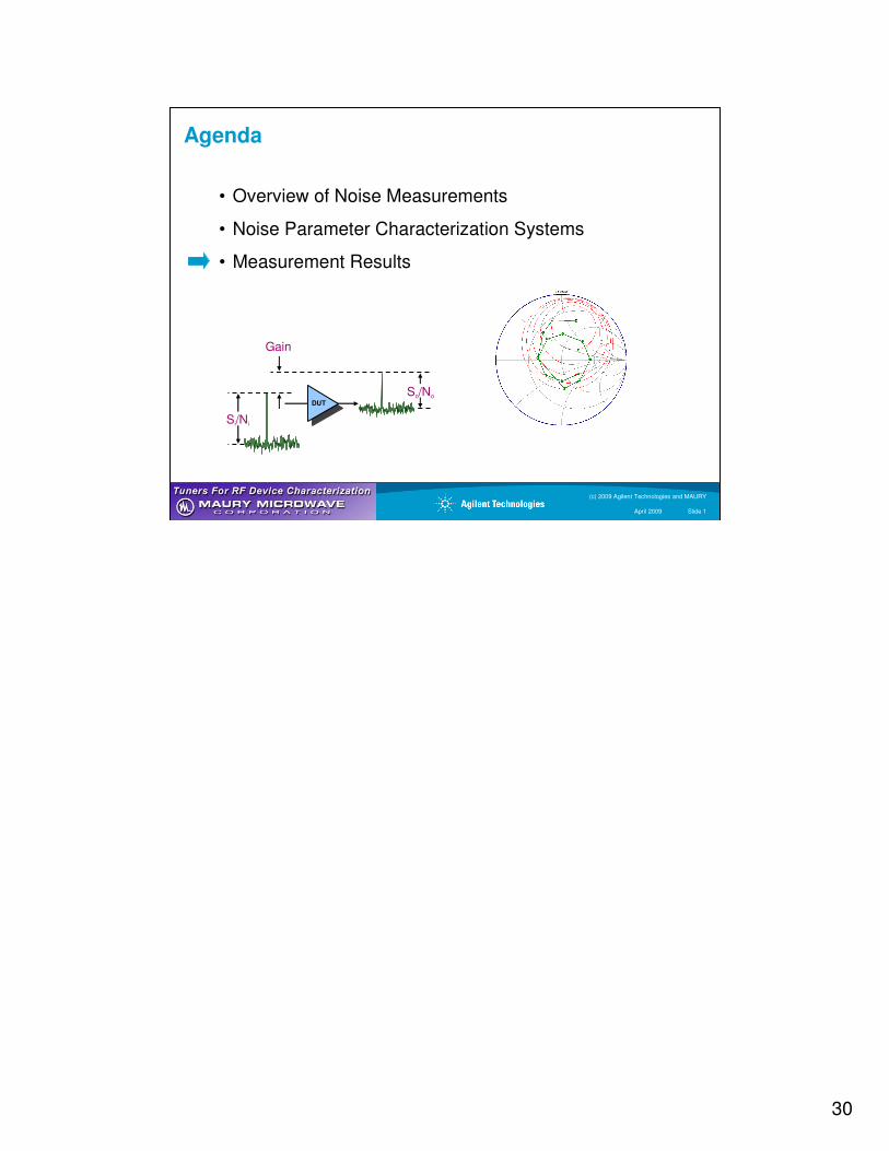
Agenda




DUT

So/No

Si/Ni

Gain


April 2009 Slide 1

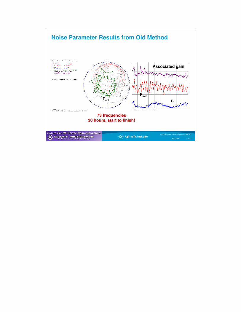
Noise Parameter Results from Old Method

Гopt

Fmin

rn

Associated gain

73 frequencies30 hours, start to finish!


April 2009 Slide 1

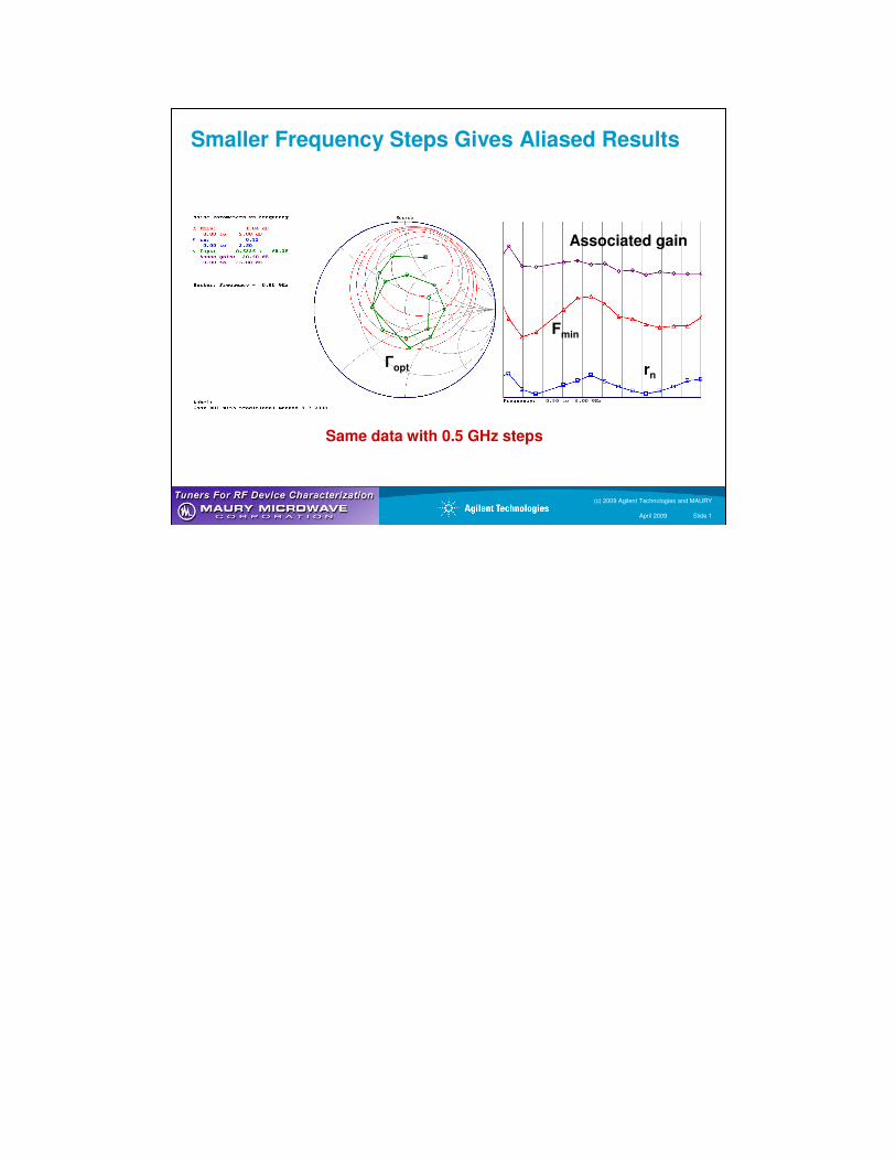
Same data with 0.5 GHz steps

Smaller Frequency Steps Gives Aliased Results

Гopt

Fmin

rn

Associated gain


April 2009 Slide 1

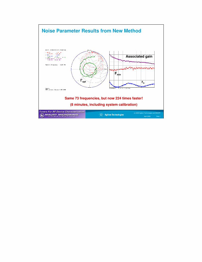
Noise Parameter Results from New Method

Гopt

Fmin

rn

Associated gain

Same 73 frequencies, but now 224 times faster!

(8 minutes, including system calibration)


April 2009 Slide 1

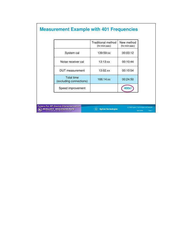
Measurement Example with 401 Frequencies

Traditional method(hr:min:sec)

New method(hr:min:sec)

System cal 139:59:xx 00:03:12

Noise receiver cal 13:13:xx 00:10:44

DUT measurement 13:02.xx 00:10:54

Total time

(excluding connections)166:14:xx 00:24:50

Speed improvement 400x!


April 2009 Slide 1

Accomplishment

• Success for motivation:

• Two orders of magnitude faster!

• Setup and measurement are much simpler!

• And, results are more accurate!


April 2009 Slide 1

How Do We Get Better Accuracy?

• Simpler setup

• Fewer cables and connections

• Always do full in-situ calibration

• Removes accumulated errors of multiple S-parameter cals

• Removes connection errors

• Minimal drift due to shorter calibration and measurement times

• Always use dense frequency selection to eliminate aliasing


April 2009 Slide 1

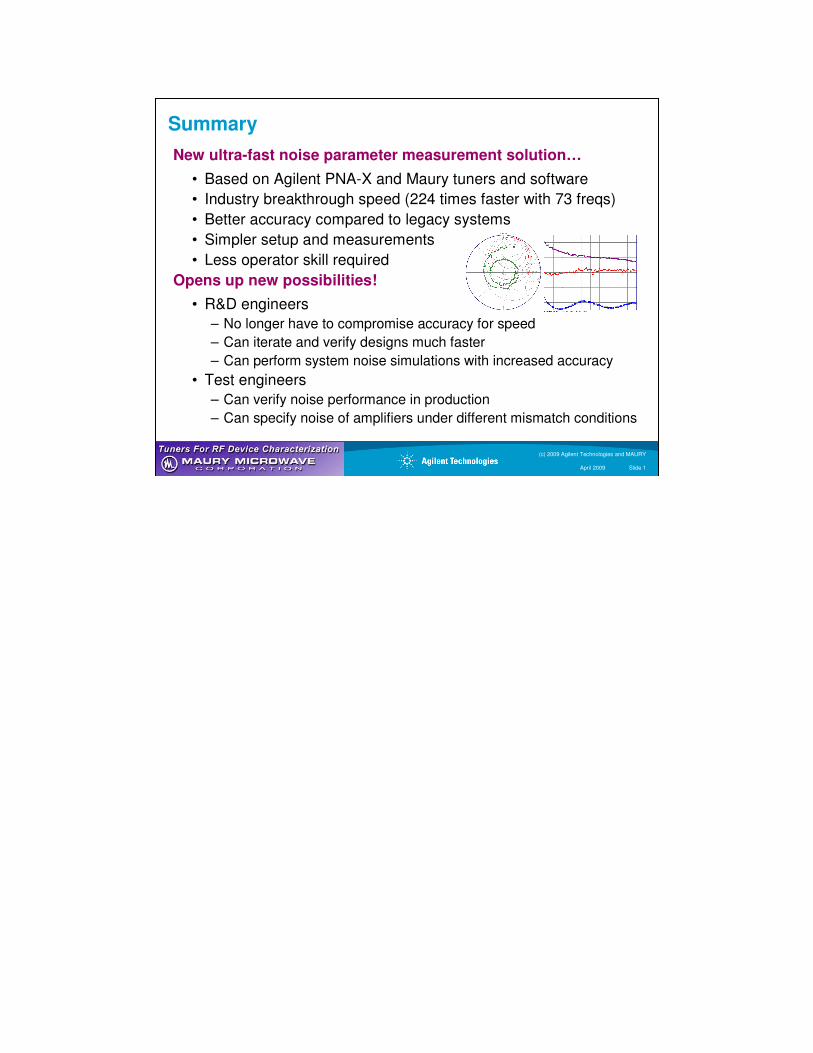
Summary

New ultra-fast noise parameter measurement solution…

• Based on Agilent PNA-X and Maury tuners and software

• Industry breakthrough speed (224 times faster with 73 freqs)

• Better accuracy compared to legacy systems

• Simpler setup and measurements

• Less operator skill required

Opens up new possibilities!

• R&D engineers

– No longer have to compromise accuracy for speed

– Can iterate and verify designs much faster

– Can perform system noise simulations with increased accuracy

• Test engineers

– Can verify noise performance in production

– Can specify noise of amplifiers under different mismatch conditions

3838


April 2009 Slide 1

.

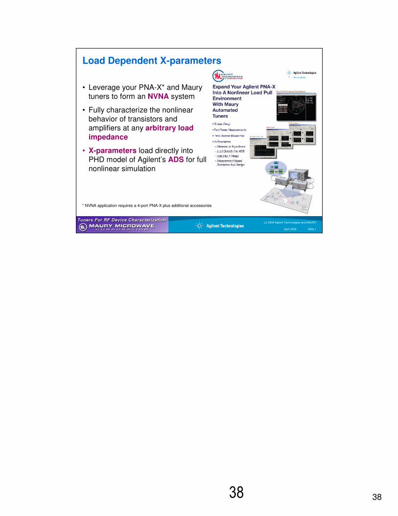
Load Dependent X-parameters

• Leverage your PNA-X* and Maury tuners to form an NVNA system

• Fully characterize the nonlinear behavior of transistors and amplifiers at any arbitrary load

impedance

• X-parameters load directly into PHD model of Agilent’s ADS for full

nonlinear simulation

* NVNA application requires a 4-port PNA-X plus additional accessories


April 2009 Slide 1

Contact Information

Call now to have your local applications consultant contact you!

Interested? Have a need? Like to know more?

Maury Microwave Sales Department• (909) 987-4715 (press “1” when prompted)

• www.maurymw.com

Agilent Technologies Test and Measurement Contact Center• (800) 829-4444• www.agilent.com/find/pnax

Documents

New Ultra-Fast Noise Parameter System Opening A … Possibilities in Noise Characterization ... 2009 Agilent Technologies and MAURY ... we can express the noise generators as current