Embed Size (px)
Citation preview
New tools in CIVA for Model Assisted Probability of Detection (MAPOD)
to support NDE reliability studies
Fabrice FOUCHER1, Roman FERNANDEZ
1, Stéphane LEBERRE2, Pierre CALMON
2
1 EXTENDE, Massy, France
2CEA Commissariat à l'Energie Atomique, Gif-sur-Yvette, France
ABSTRACT
In the context of the damage tolerance approach used to drive aircraft maintenance operations, it is
essential to demonstrate the reliability of NDE inspections in detecting structural damage. The
Probability Of Detection method, that links the probability to detect a detrimental flaw to its size is
generally used for that purpose by giving the maximum flaw size that a NDE process can miss with a
given level of probability and confidence. To be statistically valid, this approach requires a sufficient
amount of data which is often difficult (and costly) to obtain with a purely experimental approach based
on mock-up tests. Numerical simulation can be particularly useful at that stage thanks to its ability to
give a very large amount of data at a relative low cost, which constitutes the so called Model Assisted
POD approach. Recent developments have even enhanced this capacity thanks to the implementation in
CIVA simulation software of metamodels. On top of providing data for POD curves, simulations and
metamodels can be also used at the design stage to optimize inspection methods and procedures and
target a given POD for a given flaw size. It can also conduct extensive studies on parameters influence
on the result, or to achieve sensitivity analysis. This communication illustrates, with some examples
based on CIVA, how simulation can help to support NDE reliability studies in aerospace applications.
Keywords: POD, Sensitivity Analysis, Simulation, MAPOD
INTRODUCTION
The simulation plays an increasing role in NDE, allowing helping the design of inspection methods, their
qualifications or the analysis and understanding of inspection results, while reducing the number of physical mock-
ups and trials. A lot of validation efforts have been put around the CIVA software to give evidence of models
validity in order to be fully considered as a reliable element to support technical decisions and justifications [1].
In the context of NDE reliability studies, extensive parametric analyses are required in order to identify essential
parameters that can affect the NDE performance. Such studies need a large amount of data which is often difficult
and costly to obtain with a set of purely experimental results. Probability Of Detection methods, that links the
probability to detect a detrimental flaw to its size is generally used for NDE reliability evaluation in the aerospace
sector. The statistical validity of this approach is also dependent on a sufficient amount of data. Numerical
simulation tools can be particularly useful at that stage thanks to its ability to give a very large amount of data at a
relative low cost. It can also help to explore deeper and more precisely some parameters variability that can be
difficult to monitor in an experimental Design Of Experiment. In addition to classical “numerical” simulations,
“Metamodels” or “surrogate models” becomes now available, which drastically ease the capacity to generate an
even larger amount of data. For parametric and sensitivity analyses, or Model Assisted POD studies, such tools give
access to results (such as Sobol Indices, beam of POD curves, non-parametric POD curves) that simply cannot be
reached with experimental studies. This paper will illustrate the benefits of the modelling and metamodeling
approach available in the CIVA simulation platform for sensitivity and POD analyses in the context of aerospace
inspection reliability studies.
I Models implemented in CIVA software
1.1 Overview of the CIVA software modelling approach
The development of CIVA software started in the early 90s first for ultrasonic application. Then, this package
became commercially available and has started to be widely and even extensively used by the NDE industrial
community from the years 2000s, in different industrial sectors such as power industry, aerospace and
transportation, oil & gas, mechanical or steel industry.
The various modules of CIVA give access to different NDT methods and techniques: Ultrasonic Testing (UT),
Guided Waves Testing (GWT), Eddy Current Testing (ET), Radiographic Testing (RT) & Radiographic Computed
Tomography (CT). All these modules are available in the same environment, bringing to the users a unique NDT
oriented Graphical User Interface. The mathematical formulations used in the different modules often rely on semi-
analytical models. This approach allows solving a large range of applications while offering very competitive
calculation time compared with purely numerical methods (FEA, etc.). For instance, the UT module relies on a rays
theory geometrical approach to compute beam propagation (the so-called “pencil method”). The interaction with
discontinuities involves several models depending on the context. Some of them relies on semi-analytical or
analytical formulations, the Kirchhoff or GTD (which stands for “Geometrical Theory of Diffraction”) model can be
mentioned but other ones have also been implemented to cover several configurations. Such model can for instance
tackle the simulation of ultrasonic waves propagation in composite structures such as Carbon Fiber Reinforced
Polymer ones. The anisotropic nature of the composite medium is accounted for with a homogenized approach as
well as the change of fiber orientation due to the part curvature. In CIVA Eddy Current, the main part involves
Volume Integral and Boundary Element Methods to compute the field/Flaw perturbation phenomenon, which only
requires a numerical sampling of the flaw. The electromagnetic field induced in the work piece will be either
calculated based either on analytical expressions, modal approaches based on truncated regions or more numerical
Surface Integral equations depending on the complexity of the eddy current probe and the component geometry.
In order to continue the extension of the application fields of CIVA, it is sometimes necessary to rely on more
general numerical approaches (FEM, Finite Difference, etc.). To keep the benefits of the semi-analytical strategy,
the current trend within CIVA is to build hybrid models, a part of the computation being done by fast semi-
analytical models, another part being completed by numerical approach when necessary for the validity of the
results. For instance, such a coupling between semi-analytical and Finite Difference or more recently with Finite
Element are used to simulate a composite medium when a ply per ply approach is required instead of the
homogenized one mentioned above. For interested readers wishing to have more information on the models, the
following reference papers are available, [2] and [3] for the Ultrasonic tool, [4] for the Guided Waves module [5] for
the Eddy Current part, [6] for the radiographic one and [7] for the CT module. For more details on composite
modelling, another article can be mentioned [8].
1.2 Metamodeling approach in a few words
A metamodel or surrogate model can be defined as a “model of the model” or a “smart interpolator” which is built to
replace a physic-based model. The first step consists in computing a data base of simulation results for a given range
of multi parameters variation. From this data set is built the meta-model which allow ultra-fast exploration of the full
range of parameters variation. Thanks to the computational speed reached with metamodel, it becomes possible to
achieve statistical analysis on data such as sensitivity and POD studies. For instance, Sobol indices can be computed
from metamodel output in order to quantify the relative importance of influential parameters. Various Design of
Experiments methods can be selected to build the data base, based on a fixed number of computed configurations or
based on adaptive sampling. This can be a Full Factorial design (range of variation and number of values for each
parameter explicitly defined) but other drawing schemes based on pseudo random sequences of parameters value
can be also selected (Latin Hypercube Sampling, Sobol, Halton), which generally reaches a better metamodel
accuracy with a much smaller amount of computations. Adaptive Sampling consists in building the data-set by
estimating at each step the accuracy of the meta-model until reaching a given convergence criterion. Also, several
interpolators can be applied to build the metamodel from the database (Multilinear, Radial Basis function, Kriging,
etc.). Interested readers can refer to the following paper for more detailed information on the metamodels currently
implemented in the CIVA software [9].
II Background in Probability of Detection and MAPOD
2.1 POD Methodology
In the aerospace sector, the damage tolerance approach is used to drive aircraft maintenance operations. This
approach requires the knowledge of the defection performance (the reliability) of the NDE process. The Probability
Of Detection method, that links the probability to detect a detrimental flaw to its size is generally used for that
purpose by giving the maximum flaw size that a NDE process can miss with a given level of probability and
confidence. The POD methodology currently adopted by the aircraft industry is described in the Military Handbook
1823A [10]. It is based on a parametric estimation of the POD following Berens models, which is adopted also in
some ASTM standards [11, 12].
Statistical analysis is defined for two different data formats: Either binary information is only provided (defect
detected or not detected), the so-called Hit Miss approach, either the signal amplitude is recorded, the so-called « â
vs a » or « Signal response » approach. The hypotheses to be satisfied as well as the statistical analysis depend on
the selected approach.
2.2 Model Assisted POD
Determination of POD curves via a purely experimental approach requires large-scale experiments performed on
representative test-blocks containing representative defects. For instance, the MH1823a states that a minimum
amount of 40 different defects location shall exist in the trial mock-ups when a Signal response analysis is
performed, while this minimum is 60 for a Hit-Miss analysis. Then, to be representative of the “real POD”, this
experiment shall “capture” the variability of the influent parameters in real inspections.
The use of numerical simulation to determine POD curves (known as MAPOD [13]) has been a subject of research
in the past years and has been used in various industrial context (Ref [14] to [19]). Recently, efforts have been done
to fix a recognized methodology and in particular let us mention here the best practice guidance and practical
recommendations published in 2016 by International Institute of Welding [20].
The methodology, as described in this document, aims at using a numerical model which simulates the results of an
inspection in order to reproduce the impact of the variability of the influential parameters on the NDE response. The
key idea consists in introducing variations in the input parameters of the model which lead to the variability on the
output of the simulation. This variability is then analyzed to calculate the POD curve. The estimation of one POD
curve by simulation requires:
1. To define a “nominal” configuration, that is all the parameters needed for simulating one inspection. From
this nominal configuration are derived the configurations which will be computed by considering the variability of
some inputted parameters.
2. To define the characteristic parameter “a” (versus which the POD (a) is calculated) and to identify and
characterize the sources of variability which will be accounted for by the POD:
To define the “aleatory parameters” whose variability will be taken into account
To assign a statistical distribution to these parameters
3. To sample the statistical distributions of aleatory parameters and run the corresponding simulations.
4. To compute the POD curve from the set of simulated cases.
The first advantage of using numerical simulation in a POD study is to save time and budget. A second significant
advantage is the possibility offered by simulation to obtain large sets of data, investigating the effects of the
variability of numerous influential parameters. Indeed, with simulation tools, it is generally quite fast & easy and
therefore represents a quite low cost to generate the sufficient amount of data required for POD analyses. This is
even more the case when metamodels are provided. It is also possible to directly and precisely monitor parameters
variation while it is difficult to control some of them in an experimental campaign (it can be for instance difficult to
precisely monitor defects orientation and to implement them in a specific zone of the mock-up). Simulation can then
explore a wider range of parameters value which can give more credit to the POD curve. The first limitation of the
MAPOD approach is related to the use of a model which always reproduces only partially the reality. Consequently,
a natural recommendation is to evaluate the accuracy of the predictions provided by the simulation code used in the
study. A second limitation is linked to the necessity to a priori identify and characterize the sources of variability on
the result of the inspection. That means to identify the influential parameters whose variability will be investigated,
and also to have a good knowledge on the statistical distributions describing the variability of those parameters. A
third limitation is that at this stage, even if this is a subject of ongoing research, the human and organizational
factors are not accounted for by this approach.
Besides the calculation of the POD curve entirely from simulation, there are various other possible uses of simulated
data in complement to experiments. Simulation gives the possibility to help determine the most influent parameters
in a given inspection, and which defect sizes correspond to the transition zone of the POD curve. As a consequence,
simulation can be used prior to an experimental campaign in order to help defining the design of experiment as well
as efficient mock-ups, which can help mastering the costs of a POD campaign. Additionally, simulation gives
insights on the results that help understanding the physical phenomena which might be also used to help designing a
more reliable inspection procedure with a given objective of POD.
III Illustrative examples
In this section, two illustrative cases are shown to describe the tools implemented in CIVA for the POD simulation
and sensitivity analysis.
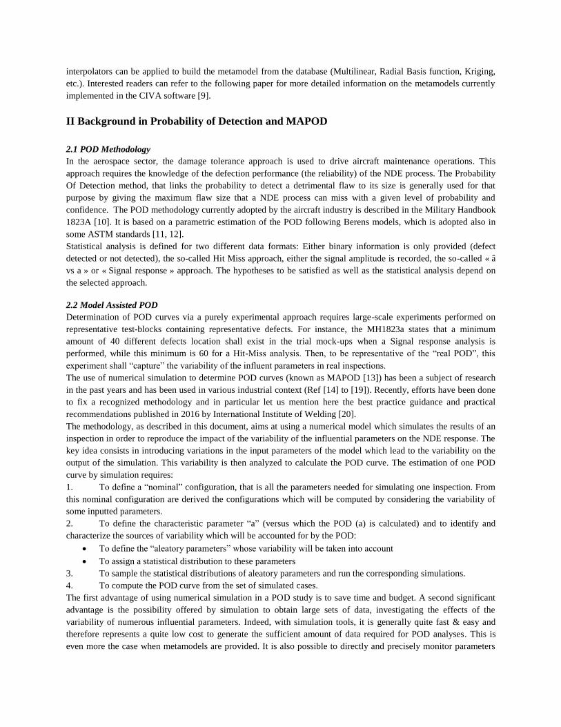
3.1 High Frequency Eddy Current Inspection Simulation
A first example corresponds to a High Frequency Eddy Current Inspection aiming at detecting surface defects in an
aluminum slab. The testing configuration is represented on the figure below. The component is an aluminum plate of
5 mm thickness. The inspection is made with a pencil sensor built with a 1.4 diameter coil and a ferrite core of 5mm
height working in absolute mode. The operating frequency is 1MHz. Surface defects are modelled with thin
parallelepiped notches. The configuration shown below represents a reference defect of 1mm height, an aperture of
50 microns and a length of 10mm. The figure shows the configuration as well as the simulated signal obtained
(impedance plane and X-Y curve).
Figure 1: High Frequency Eddy current model on an aluminum slab, results obtained on a reference defect
The prior list of influent parameters for this inspection included the specimen conductivity, the coil diameter, the
ferrite core permeability, the lift-off, the orientation of the probe (normal to the surface or with a tilt angle), the
scanning path over the defect, and the width and height of the defects. After a first impact analysis, 4 main essential
variables were kept in the design of experiment with the following range of variation:
Lift-off [0.15mm; 0.5mm]
Sensor orientation [-5°; +5°]
Defect height [0.5mm; 3mm]
Defect aperture [0.03mm; 0.07mm]
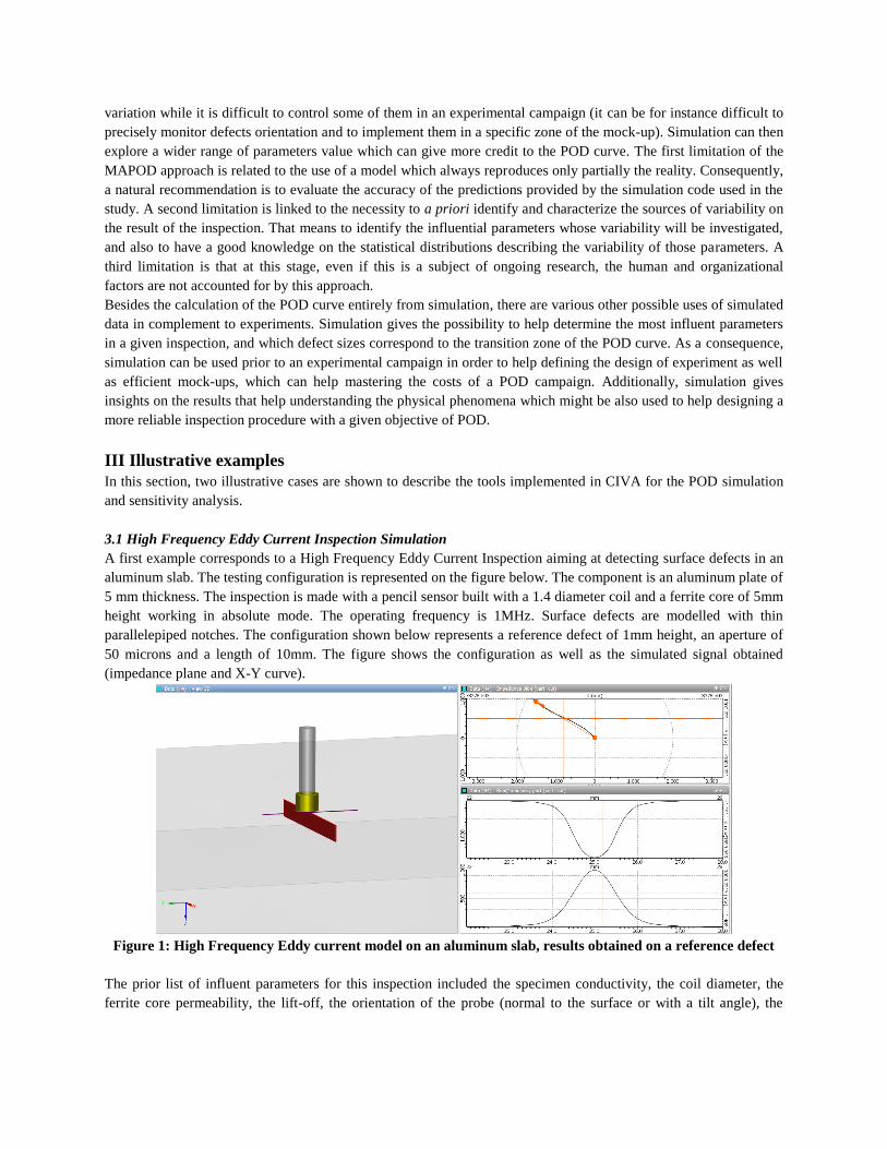
The defect length has been also of course investigated and has been even selected as the characteristic parameter, i.e.
the one which will represent the defect size “a” for the future POD analysis. A metamodel has been calculated based
on a sample of 500 computations. The total computation time was about 20 hours on a standard PC (about 2 minutes
for each case scan). The following graph (so-called “parallel plot”) represents the map of the different parameters
computed in order to build the metamodel database and an overview of the results obtained for the whole cases. The
5 first columns represent the values assigned to the variable input parameters (a Sobol sampling scheme has been
used here) and the 6th
column on the right shows the corresponding results (amplitude of sensor signal generally).
This parallel plot also helps identifying at a glance for instance which cases give the lowest signals or how is
affected the output variability when you limit one or several parameters to a given range:
a) b)
Figure 2: Parallel plot of the simulations (5 first columns: parameter values; 6th
column: Signal amplitude)
a) All Cases, b) highlighted cases for a limited range of one parameter
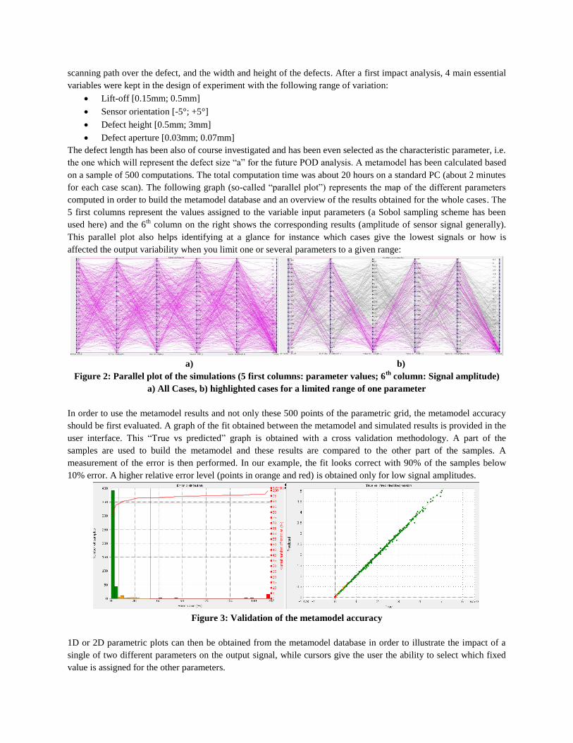
In order to use the metamodel results and not only these 500 points of the parametric grid, the metamodel accuracy
should be first evaluated. A graph of the fit obtained between the metamodel and simulated results is provided in the
user interface. This “True vs predicted” graph is obtained with a cross validation methodology. A part of the
samples are used to build the metamodel and these results are compared to the other part of the samples. A
measurement of the error is then performed. In our example, the fit looks correct with 90% of the samples below
10% error. A higher relative error level (points in orange and red) is obtained only for low signal amplitudes.
Figure 3: Validation of the metamodel accuracy
1D or 2D parametric plots can then be obtained from the metamodel database in order to illustrate the impact of a
single of two different parameters on the output signal, while cursors give the user the ability to select which fixed
value is assigned for the other parameters.
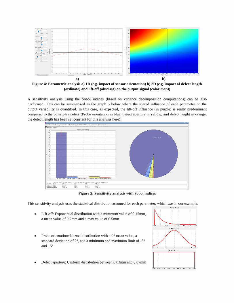
a) b)
Figure 4: Parametric analysis a) 1D (e.g. impact of sensor orientation) b) 2D (e.g. impact of defect length
(ordinate) and lift-off (abscissa) on the output signal (color map))
A sensitivity analysis using the Sobol indices (based on variance decomposition computations) can be also
performed. This can be summarized as the graph 5 below where the shared influence of each parameter on the
output variability is quantified. In this case, as expected, the lift-off influence (in purple) is really predominant
compared to the other parameters (Probe orientation in blue, defect aperture in yellow, and defect height in orange,
the defect length has been set constant for this analysis here):
Figure 5: Sensitivity analysis with Sobol indices
This sensitivity analysis uses the statistical distribution assumed for each parameter, which was in our example:
Lift-off: Exponential distribution with a minimum value of 0.15mm,
a mean value of 0.2mm and a max value of 0.5mm
Probe orientation: Normal distribution with a 0° mean value, a
standard deviation of 2°, and a minimum and maximum limit of -5°
and +5°
Defect aperture: Uniform distribution between 0.03mm and 0.07mm
Defect height: Uniform distribution between 0.5mm and 3mm
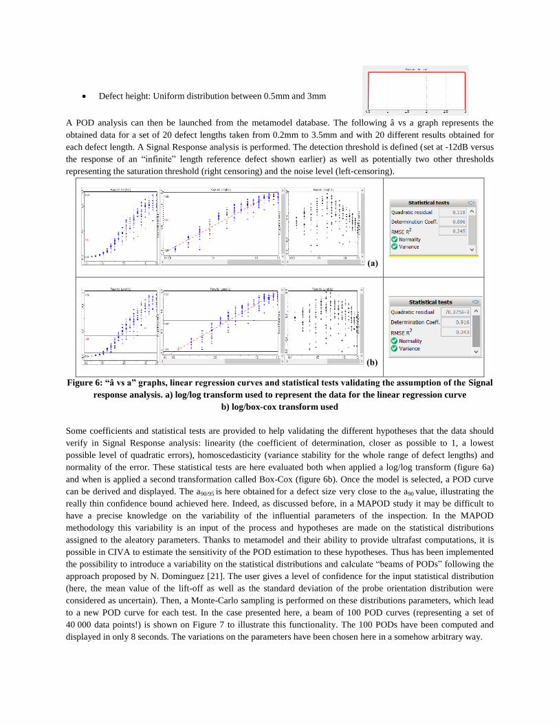
A POD analysis can then be launched from the metamodel database. The following â vs a graph represents the
obtained data for a set of 20 defect lengths taken from 0.2mm to 3.5mm and with 20 different results obtained for
each defect length. A Signal Response analysis is performed. The detection threshold is defined (set at -12dB versus
the response of an “infinite” length reference defect shown earlier) as well as potentially two other thresholds
representing the saturation threshold (right censoring) and the noise level (left-censoring).
(a)
(b)
Figure 6: “â vs a” graphs, linear regression curves and statistical tests validating the assumption of the Signal
response analysis. a) log/log transform used to represent the data for the linear regression curve
b) log/box-cox transform used
Some coefficients and statistical tests are provided to help validating the different hypotheses that the data should
verify in Signal Response analysis: linearity (the coefficient of determination, closer as possible to 1, a lowest
possible level of quadratic errors), homoscedasticity (variance stability for the whole range of defect lengths) and
normality of the error. These statistical tests are here evaluated both when applied a log/log transform (figure 6a)
and when is applied a second transformation called Box-Cox (figure 6b). Once the model is selected, a POD curve
can be derived and displayed. The a90/95 is here obtained for a defect size very close to the a90 value, illustrating the
really thin confidence bound achieved here. Indeed, as discussed before, in a MAPOD study it may be difficult to
have a precise knowledge on the variability of the influential parameters of the inspection. In the MAPOD
methodology this variability is an input of the process and hypotheses are made on the statistical distributions
assigned to the aleatory parameters. Thanks to metamodel and their ability to provide ultrafast computations, it is
possible in CIVA to estimate the sensitivity of the POD estimation to these hypotheses. Thus has been implemented
the possibility to introduce a variability on the statistical distributions and calculate “beams of PODs” following the
approach proposed by N. Dominguez [21]. The user gives a level of confidence for the input statistical distribution
(here, the mean value of the lift-off as well as the standard deviation of the probe orientation distribution were
considered as uncertain). Then, a Monte-Carlo sampling is performed on these distributions parameters, which lead
to a new POD curve for each test. In the case presented here, a beam of 100 POD curves (representing a set of
40 000 data points!) is shown on Figure 7 to illustrate this functionality. The 100 PODs have been computed and
displayed in only 8 seconds. The variations on the parameters have been chosen here in a somehow arbitrary way.
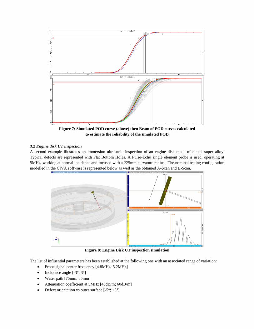
Figure 7: Simulated POD curve (above) then Beam of POD curves calculated
to estimate the reliability of the simulated POD
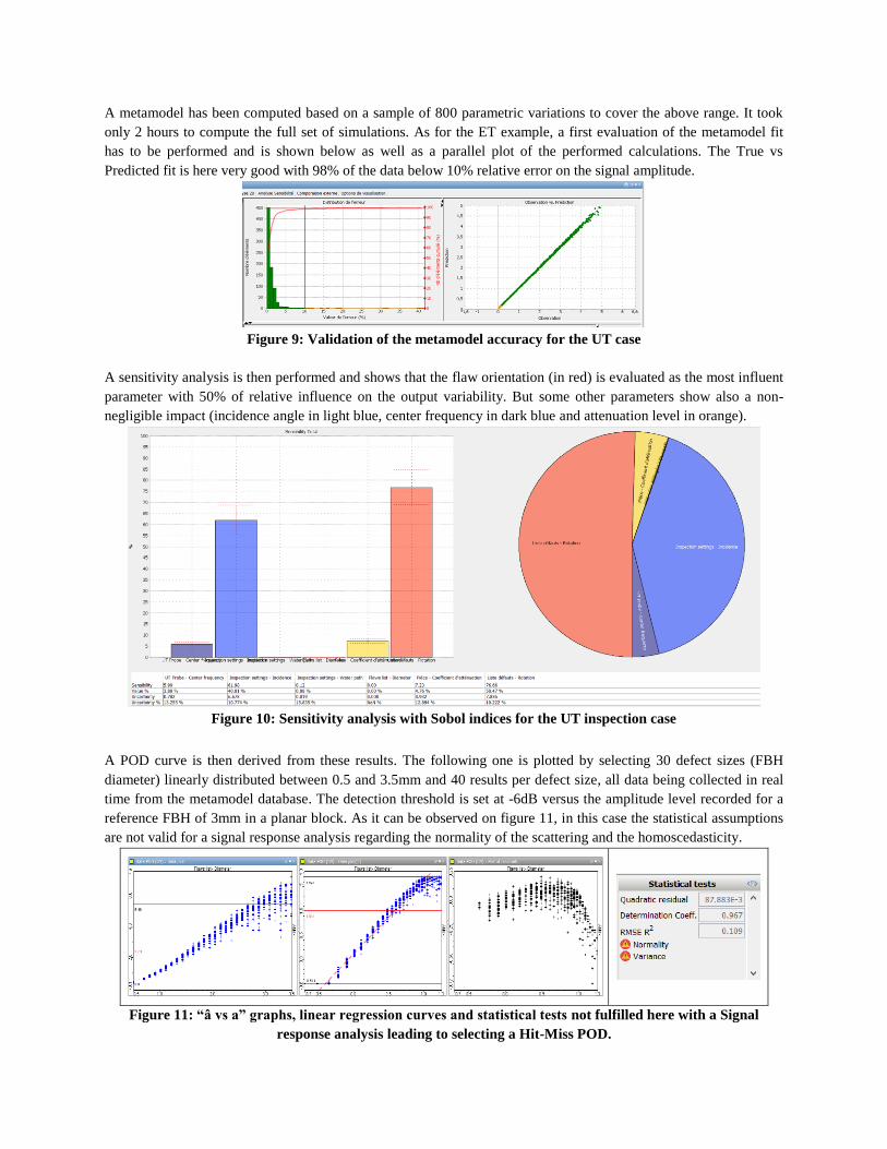
3.2 Engine disk UT inspection
A second example illustrates an immersion ultrasonic inspection of an engine disk made of nickel super alloy.
Typical defects are represented with Flat Bottom Holes. A Pulse-Echo single element probe is used, operating at
5MHz, working at normal incidence and focused with a 225mm curvature radius. The nominal testing configuration
modelled in the CIVA software is represented below as well as the obtained A-Scan and B-Scan.
Figure 8: Engine Disk UT inspection simulation
The list of influential parameters has been established at the following one with an associated range of variation:
Probe signal center frequency [4.8MHz; 5.2MHz]
Incidence angle [-3°; 3°]
Water path [75mm; 85mm]
Attenuation coefficient at 5MHz [40dB/m; 60dB/m]
Defect orientation vs outer surface [-5°; +5°]
A metamodel has been computed based on a sample of 800 parametric variations to cover the above range. It took
only 2 hours to compute the full set of simulations. As for the ET example, a first evaluation of the metamodel fit
has to be performed and is shown below as well as a parallel plot of the performed calculations. The True vs
Predicted fit is here very good with 98% of the data below 10% relative error on the signal amplitude.
Figure 9: Validation of the metamodel accuracy for the UT case
A sensitivity analysis is then performed and shows that the flaw orientation (in red) is evaluated as the most influent
parameter with 50% of relative influence on the output variability. But some other parameters show also a non-
negligible impact (incidence angle in light blue, center frequency in dark blue and attenuation level in orange).
Figure 10: Sensitivity analysis with Sobol indices for the UT inspection case
A POD curve is then derived from these results. The following one is plotted by selecting 30 defect sizes (FBH
diameter) linearly distributed between 0.5 and 3.5mm and 40 results per defect size, all data being collected in real
time from the metamodel database. The detection threshold is set at -6dB versus the amplitude level recorded for a
reference FBH of 3mm in a planar block. As it can be observed on figure 11, in this case the statistical assumptions
are not valid for a signal response analysis regarding the normality of the scattering and the homoscedasticity.
Figure 11: “â vs a” graphs, linear regression curves and statistical tests not fulfilled here with a Signal
response analysis leading to selecting a Hit-Miss POD.
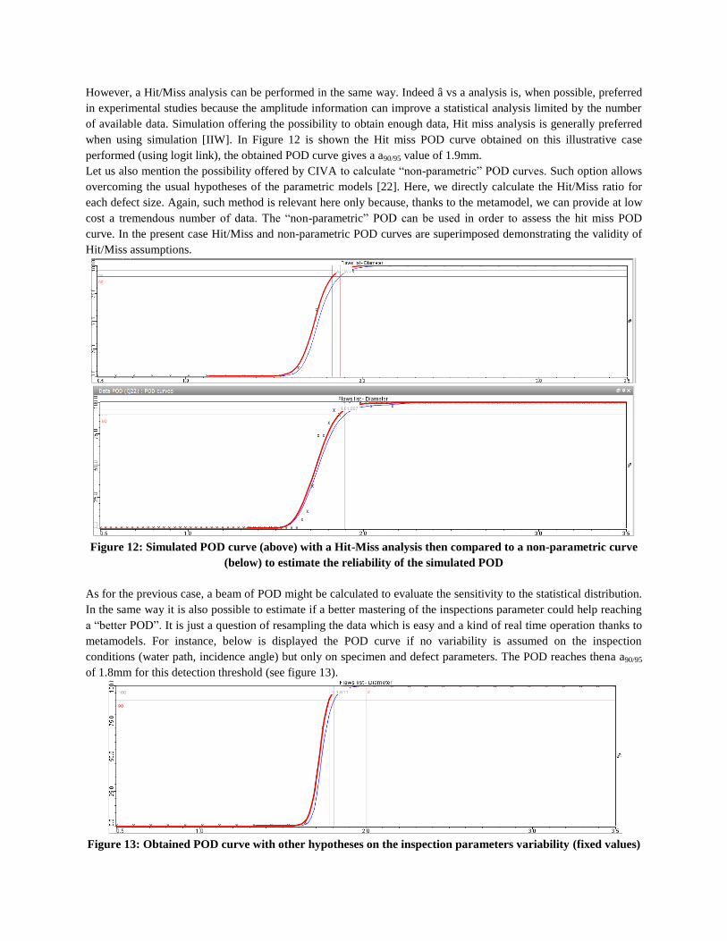
However, a Hit/Miss analysis can be performed in the same way. Indeed â vs a analysis is, when possible, preferred
in experimental studies because the amplitude information can improve a statistical analysis limited by the number
of available data. Simulation offering the possibility to obtain enough data, Hit miss analysis is generally preferred
when using simulation [IIW]. In Figure 12 is shown the Hit miss POD curve obtained on this illustrative case
performed (using logit link), the obtained POD curve gives a a90/95 value of 1.9mm.
Let us also mention the possibility offered by CIVA to calculate “non-parametric” POD curves. Such option allows
overcoming the usual hypotheses of the parametric models [22]. Here, we directly calculate the Hit/Miss ratio for
each defect size. Again, such method is relevant here only because, thanks to the metamodel, we can provide at low
cost a tremendous number of data. The “non-parametric” POD can be used in order to assess the hit miss POD
curve. In the present case Hit/Miss and non-parametric POD curves are superimposed demonstrating the validity of
Hit/Miss assumptions.
Figure 12: Simulated POD curve (above) with a Hit-Miss analysis then compared to a non-parametric curve
(below) to estimate the reliability of the simulated POD
As for the previous case, a beam of POD might be calculated to evaluate the sensitivity to the statistical distribution.
In the same way it is also possible to estimate if a better mastering of the inspections parameter could help reaching
a “better POD”. It is just a question of resampling the data which is easy and a kind of real time operation thanks to
metamodels. For instance, below is displayed the POD curve if no variability is assumed on the inspection
conditions (water path, incidence angle) but only on specimen and defect parameters. The POD reaches thena a90/95
of 1.8mm for this detection threshold (see figure 13).
Figure 13: Obtained POD curve with other hypotheses on the inspection parameters variability (fixed values)
CONCLUSION
Simulation tools gathered in the CIVA platform provide an efficient solution to support NDE reliability study. In
particular, the recent introduction of metamodels offers new possibilities such as real-time resampling of the data
which is particularly useful to perform sensitivity analysis (Sobol indices evaluation) or advanced POD analysis
(assessment of statistical models, beam of POD curves, or even non parametric POD curves, etc.). Simulation can
then be used either to help defining the design of Experiment for an experimental campaign, to compute directly the
POD curves or to give insights for inspection method optimization to reach a targeted value of POD.
REFERENCES
(1) F. Foucher, S. Lonné, G. Toullelan, S. Mahaut, S. Chatillon, 2018, An overwiew of validation campaigns of the
CIVA simulation software, ECNDT.
(2) S. Mahaut, S. Chatillon, M. Darmon, N. Leymarie and R. Raillon, 2009, An overview of UT beam propagation
and flaw scattering models in CIVA, QNDE.
(3) M. Darmon, S. Chatillon, 2013, Main Features of a Complete Ultrasonic Measurement Model: Formal Aspects
of Modeling of Both Transducers Radiation and Ultrasonic Flaws Responses, Open Journal of Acoustics,
Vol.3 No.3A, http://file.scirp.org/Html/8-1610079_36873.htm#txtF2.
(4) V. Baronian, A. Lhémery, K. Jezzine, 2010, Hybrid SAFE/FE simulation of inspections of elastic waveguides
containing several local discontinuities, QNDE.
(5) G. Pichenot et al., 2005, Development of a 3D electromagnetic model for eddy current tubing inspection:
Application to steam generator tubing, QNDE.
(6) J.Tabary, P. Hugonnard, A.Schumm, R. Fernandez, 2008, Simulation studies of radiographic inspections with
Civa, WCNDT.
(7) R. Fernandez, S.A. Legoupil, M. Costin, A. Leveque, 2012, CIVA Computed Tomography Modeling, WCNDT.
(8) K. Jezzine et al, 2017, Modeling approaches for the simulation of ultrasonic inspections of anisotropic
composite structures in the CIVA software platform, QNDE.
(9) R. Miorelli et al, Database generation and exploitation for efficient and intensive simulation studies, AIP
Conference Proceedings, Volume 1706 (2016)
(10) USA Department of Defense Handbook, 2009, MIL-HDBK-1823-A, NDE system reliability assessment.
(11) ASTM, 2012, E2862-12: Standard practice for probability of detection analysis for hit/miss data.
(12) ASTM, 2012, E3023-15: Standard practice for probability of detection analysis for â versus a data.
(13) B. Thompson et al, 2009, Recent Advances in Model-Assisted Probability of Detection, European-American
Workshop on reliability in NDE.
(14) Aldrin, J.C., Knopp, J.S., Lindgren, E.A., Jata, K.V., Model-assisted probability of detection evaluation for
eddy current inspection of fastener sites, AIP Proceedings, Volume 1096, 2009, Pages 1784-1791
(15) F. Jenson et al, 2010, Simulation supported POD: methodology and HFET validation case, QNDE
(16) Dominguez, N., Feuillard, V., Jenson, F., Willaume P., 2012, Simulation assisted POD of a Phased Array
Ultrasonic Inspection in Manufacturing, Rev. of Prog. In QNDE, Vol 31 (2012) pages 1765-1772
(17) B. Chapuis et al, 2014, Simulation supported POD curves for automated UT of pipeline girth welds, welding in
the world, V58, 433-441
(18) M. Pavlovic et al, 2016, Reliability Analysis of the Ultrasonic Inspection System for the Inspection of Hollow
Railway Axles, WCNDT.
(19) G. Ribay et al, 2016, Model-based POD study of manual ultrasound inspection and sensitivity analysis using
metamodel, AIP Conf. Proc. 1706 (2016)
(18) N. Dominguez et al, 2014, POD Evaluation using simulation: PAUT case on a complex geometry part, AIP
Conf. Proc. 1581, 2031

(20a) B. Chapuis, P. Calmon, F. Jenson, 2016, Best practices for the use of Simulation in POD Curves Estimation,
IIW Collection.
(20b) P. Calmon and al, 2016, The use of simulation in POD curves estimation: An overview of the IIW best
practices proposal, WCNDT
(21) N. Dominguez et al, 2013, A new approach of confidence in POD determination using simulation, QNDE.
(22) Spencer, F.W., Nonparametric Pod Estimation for Hit/miss Data: a Goodness of Fit Comparison for
parametric Models, Review of Quantitative Nondestructive Evaluation, AIP Conference Proceedings, 2011

![Validation of CIVA RT module for nuclear applications 1* 1 3 ......In the CIVA simulation platform, radiographic film modelling is based on the European ISO 11699-1 standard [8] as](https://img.pdfslide.us/doc/110x75/612a1f0e40a76429a0366a0b/validation-of-civa-rt-module-for-nuclear-applications-1-1-3-in-the-civa.jpg)