NEW MODELS FOR HIGH AND NEW MODELS FOR HIGH AND

LOW FREQUENCY VOLATILITYLOW FREQUENCY VOLATILITY Robert EngleRobert Engle

NYU Salomon CenterNYU Salomon Center

Derivatives Research ProjectDerivatives Research Project

FORECASTING WITH FORECASTING WITH GARCHGARCH

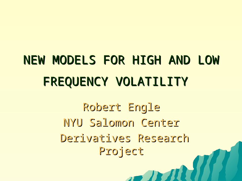
DJ RETURNSDJ RETURNS

-.08

-.06

-.04

-.02

.00

.02

.04

.06

.08

1990 1992 1994 1996 1998 2000 2002 2004

DJRET

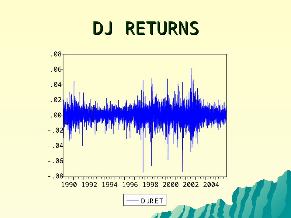
DOW JONES SINCE 1990DOW JONES SINCE 1990Dependent Variable: DJRETMethod: ML - ARCH (Marquardt) - Normal distributionDate: 01/13/05 Time: 14:30Sample: 15362 19150Included observations: 3789Convergence achieved after 14 iterationsVariance backcast: ONGARCH = C(2) + C(3)*RESID(-1)^2 + C(4)*GARCH(-1)

Coefficient Std. Error z-Statistic Prob.

C 0.000552 0.000135 4.093478 0.0000

Variance Equation

C 9.89E-07 1.84E-07 5.380913 0.0000RESID(-1)^2 0.066409 0.004478 14.82844 0.0000GARCH(-1) 0.924912 0.005719 161.7365 0.0000

R-squared -0.000370 Mean dependent var 0.000356Adjusted R-squared -0.001163 S.D. dependent var 0.010194S.E. of regression 0.010200 Akaike info criterion -6.557778Sum squared resid 0.393815 Schwarz criterion -6.551191Log likelihood 12427.71 Durbin-Watson stat 1.985498

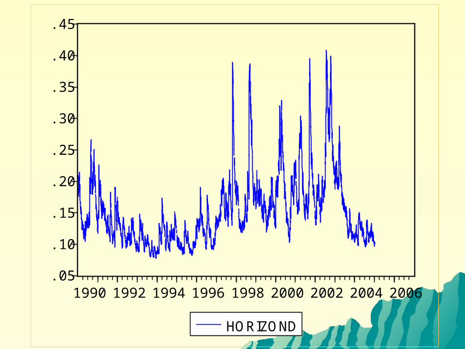
.05

.10

.15

.20

.25

.30

.35

.40

.45

1990 1992 1994 1996 1998 2000 2002 2004 2006

HORIZOND

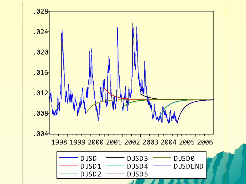
.004

.008

.012

.016

.020

.024

.028

1998 1999 2000 2001 2002 2003 2004 2005 2006

DJSDDJSD1DJSD2

DJSD3DJSD4DJSD5

DJSD0DJSDEND

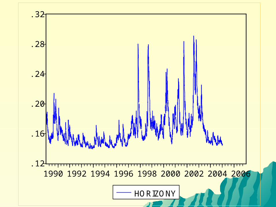
.12

.16

.20

.24

.28

.32

1990 1992 1994 1996 1998 2000 2002 2004 2006

HORIZONY

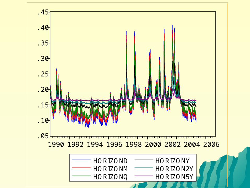
.05

.10

.15

.20

.25

.30

.35

.40

.45

1990 1992 1994 1996 1998 2000 2002 2004 2006

HORIZONDHORIZONMHORIZONQ

HORIZONYHORIZON2YHORIZON5Y

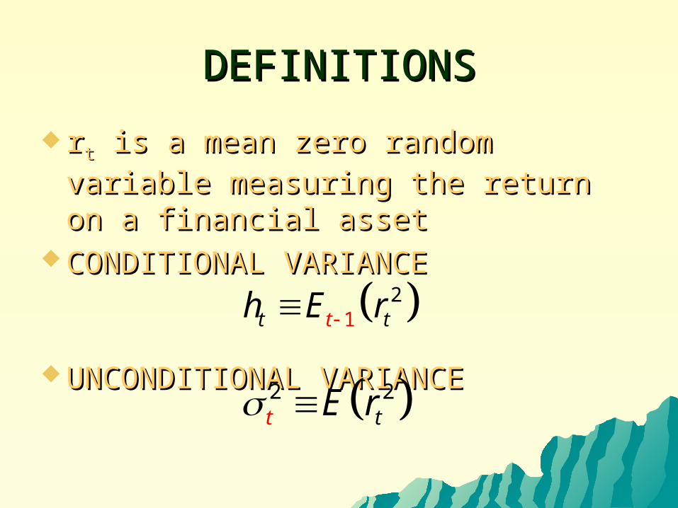
DEFINITIONSDEFINITIONS

rrtt is a mean zero random variable is a mean zero random variable measuring the return on a financial measuring the return on a financial assetasset

CONDITIONAL VARIANCE CONDITIONAL VARIANCE

UNCONDITIONAL VARIANCE UNCONDITIONAL VARIANCE

12

t tth E r

2 2tt E r

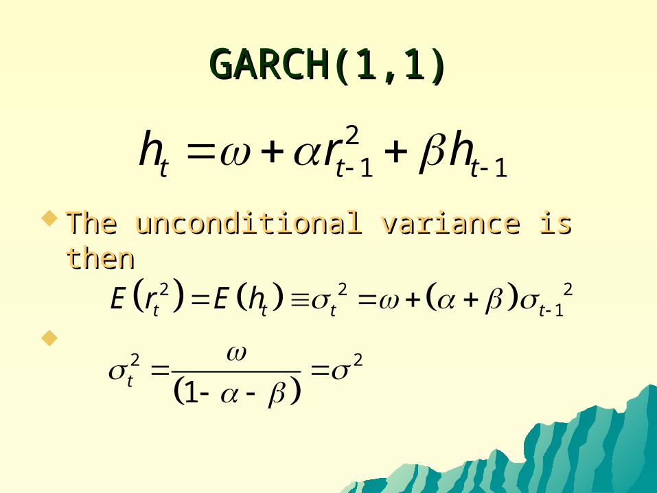
GARCH(1,1)GARCH(1,1)

The unconditional variance is then The unconditional variance is then

21 1t t th r h

2 2 21

2 2

1

t t t t

t

E r E h

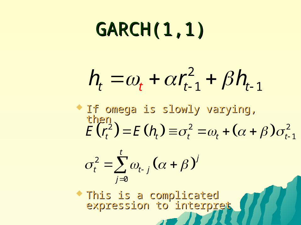
GARCH(1,1)GARCH(1,1)

If omega is slowly varying, then If omega is slowly varying, then

This is a complicated expression This is a complicated expression to interpret to interpret

21 1t t tth r h

2 2 21

2

0

t t t t t

tj

t t jj

E r E h

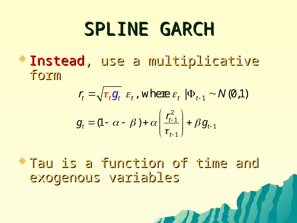
SPLINE GARCHSPLINE GARCH

InsteadInstead, use a multiplicative form, use a multiplicative form

Tau is a function of time and Tau is a function of time and exogenous variablesexogenous variables

1, where | (0,1)t t t tt tr g N 2

11

1

(1 ) tt t

t

rg g

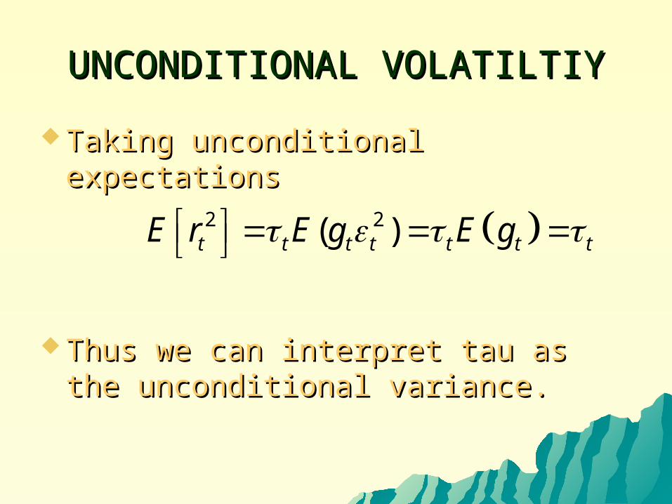
UNCONDITIONAL VOLATILTIYUNCONDITIONAL VOLATILTIY

Taking unconditional expectationsTaking unconditional expectations

Thus we can interpret tau as the Thus we can interpret tau as the unconditional variance.unconditional variance.

2 2( )t t t t t t tE r E g E g

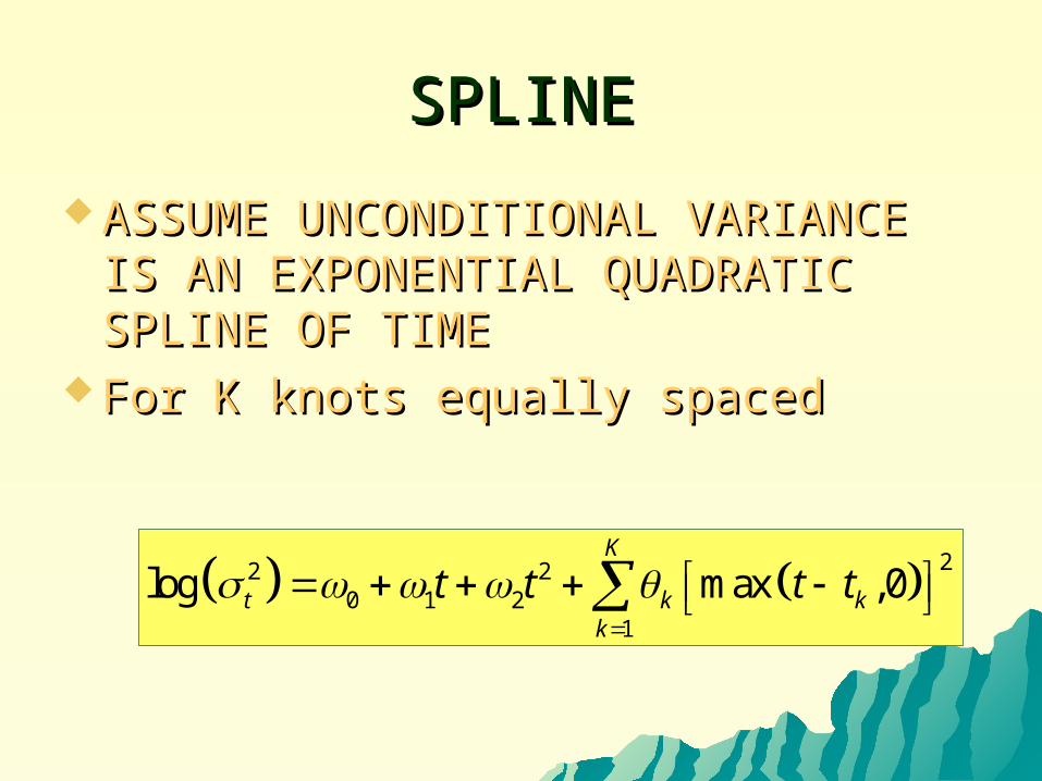
SPLINESPLINE

ASSUME UNCONDITIONAL VARIANCE ASSUME UNCONDITIONAL VARIANCE IS AN EXPONENTIAL QUADRATIC IS AN EXPONENTIAL QUADRATIC SPLINE OF TIMESPLINE OF TIME

For K knots equally spacedFor K knots equally spaced

22 20 1 2

1

log max ,0K

t k kk

t t t t

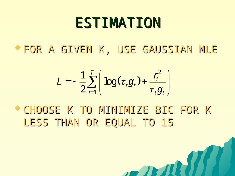
ESTIMATIONESTIMATION

FOR A GIVEN K, USE GAUSSIAN MLEFOR A GIVEN K, USE GAUSSIAN MLE

CHOOSE K TO MINIMIZE BIC FOR K CHOOSE K TO MINIMIZE BIC FOR K LESS THAN OR EQUAL TO 15LESS THAN OR EQUAL TO 15

2

1

1log

2

Tt

t tt t t

rL g

g

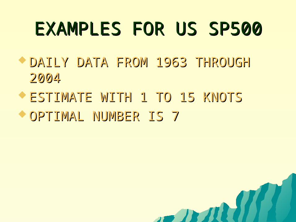
EXAMPLES FOR US SP500EXAMPLES FOR US SP500

DAILY DATA FROM 1963 THROUGH DAILY DATA FROM 1963 THROUGH 20042004

ESTIMATE WITH 1 TO 15 KNOTSESTIMATE WITH 1 TO 15 KNOTS OPTIMAL NUMBER IS 7OPTIMAL NUMBER IS 7

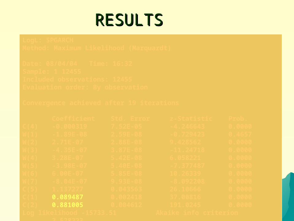
RESULTSRESULTSLogL: SPGARCHMethod: Maximum Likelihood (Marquardt)

Date: 08/04/04 Time: 16:32Sample: 1 12455Included observations: 12455Evaluation order: By observationConvergence achieved after 19 iterations

Coefficient Std. Errorz-Statistic Prob. C(4) -0.000319 7.52E-05 -4.246643 0.0000W(1) -1.89E-08 2.59E-08 -0.729423 0.4657W(2) 2.71E-07 2.88E-08 9.428562 0.0000W(3) -4.35E-07 3.87E-08 -11.24718 0.0000W(4) 3.28E-07 5.42E-08 6.058221 0.0000W(5) -3.98E-07 5.40E-08 -7.377487 0.0000W(6) 6.00E-07 5.85E-08 10.26339 0.0000W(7) -8.04E-07 9.93E-08 -8.092208 0.0000C(5) 1.137277 0.043563 26.10666 0.0000C(1) 0.089487 0.002418 37.00816 0.0000C(2) 0.881005 0.004612 191.0245 0.0000Log likelihood -15733.51 Akaike info criterion 2.528223Avg. log likelihood -1.263228 Schwarz criterion 2.534785Number of Coefs. 11 Hannan-Quinn criter. 2.530420

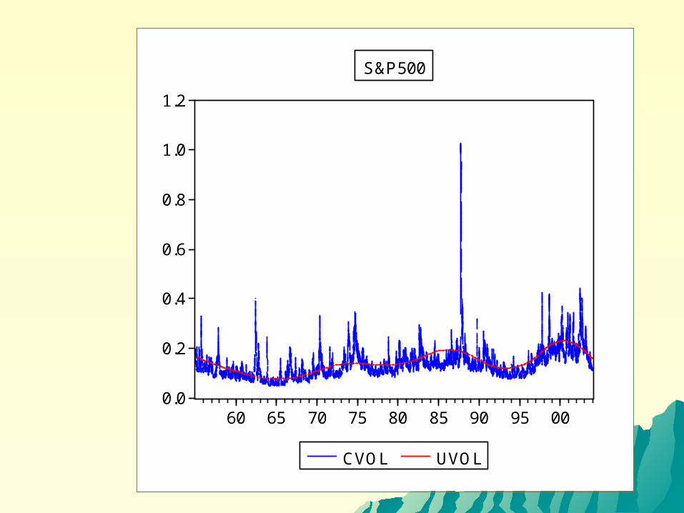
0.0

0.2

0.4

0.6

0.8

1.0

1.2

60 65 70 75 80 85 90 95 00

CVOL UVOL

S&P500

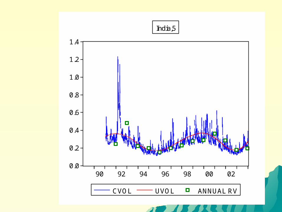
0.0

0.2

0.4

0.6

0.8

1.0

1.2

1.4

90 92 94 96 98 00 02

CVOL UVOL ANNUAL RV

India,5

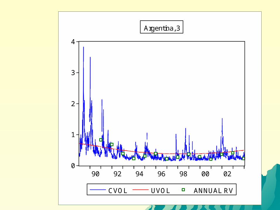
0

1

2

3

4

90 92 94 96 98 00 02

CVOL UVOL ANNUAL RV

Argentina, 3

0.0

0.2

0.4

0.6

0.8

1.0

90 92 94 96 98 00 02

CVOL UVOL ANNUAL RV

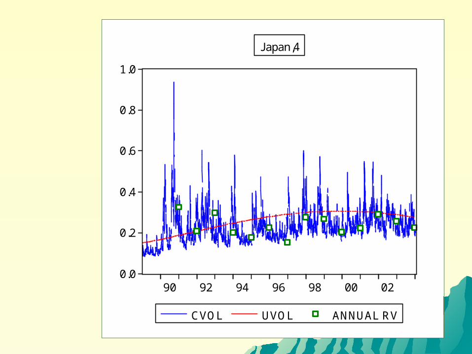
Japan,4

0.0

0.5

1.0

1.5

2.0

2.5

3.0

90 92 94 96 98 00 02

CVOL UVOL ANNUAL RV

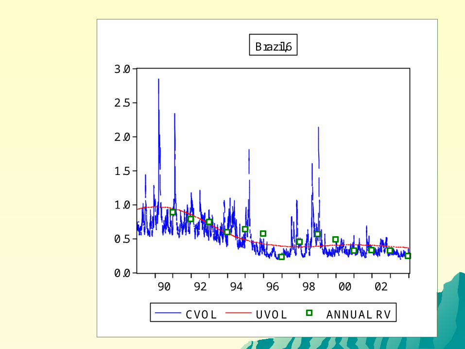
Brazil,6

.0

.1

.2

.3

.4

.5

.6

.7

.8

.9

90 92 94 96 98 00 02

CVOL UVOL ANNUAL RV

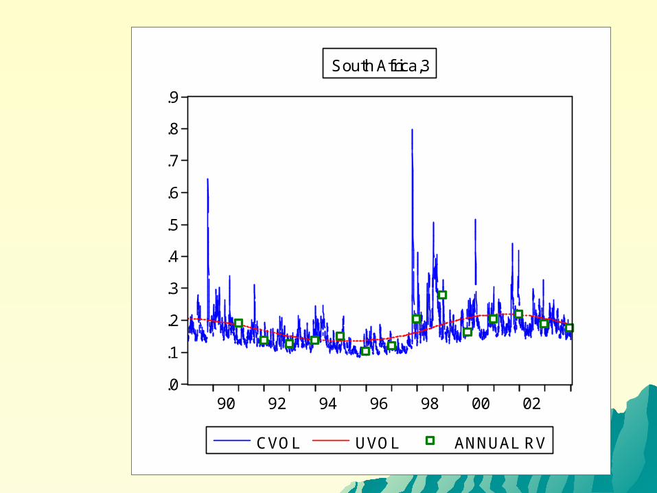
South Africa,3

0.1

0.2

0.3

0.4

0.5

0.6

0.7

0.8

0.9

1.0

90 92 94 96 98 00 02

CVOL UVOL ANNUAL RV

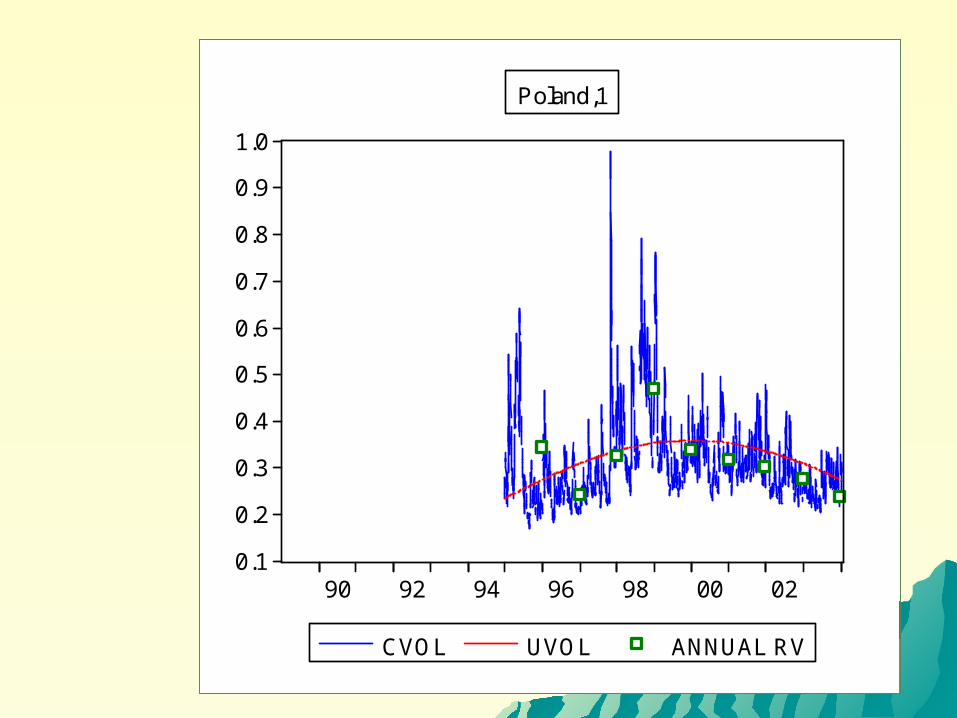
Poland,1

ESTIMATIONESTIMATION

Volatility is regressed against explanatory Volatility is regressed against explanatory variables with observations for countries variables with observations for countries and years.and years.

Within a country residuals are auto-Within a country residuals are auto-correlated due to spline smoothing. Hence correlated due to spline smoothing. Hence use SUR.use SUR.

Volatility responds to global news so there Volatility responds to global news so there is a time dummy for each year.is a time dummy for each year.

Unbalanced panelUnbalanced panel

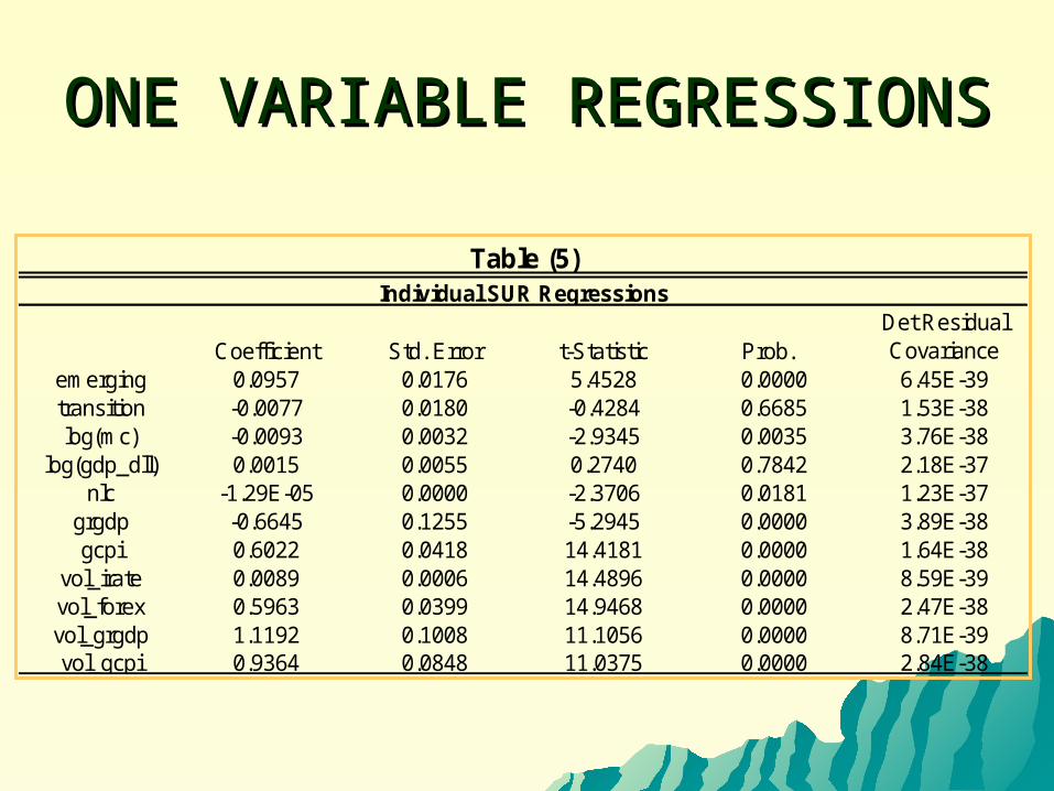
ONE VARIABLE ONE VARIABLE REGRESSIONSREGRESSIONS

Coefficient Std. Error t-Statistic Prob. Det Residual Covariance

emerging 0.0957 0.0176 5.4528 0.0000 6.45E-39transition -0.0077 0.0180 -0.4284 0.6685 1.53E-38log(mc) -0.0093 0.0032 -2.9345 0.0035 3.76E-38

log(gdp_dll) 0.0015 0.0055 0.2740 0.7842 2.18E-37nlc -1.29E-05 0.0000 -2.3706 0.0181 1.23E-37

grgdp -0.6645 0.1255 -5.2945 0.0000 3.89E-38gcpi 0.6022 0.0418 14.4181 0.0000 1.64E-38

vol_irate 0.0089 0.0006 14.4896 0.0000 8.59E-39vol_forex 0.5963 0.0399 14.9468 0.0000 2.47E-38vol_grgdp 1.1192 0.1008 11.1056 0.0000 8.71E-39vol_gcpi 0.9364 0.0848 11.0375 0.0000 2.84E-38

Individual SUR Regressions

Table (5)

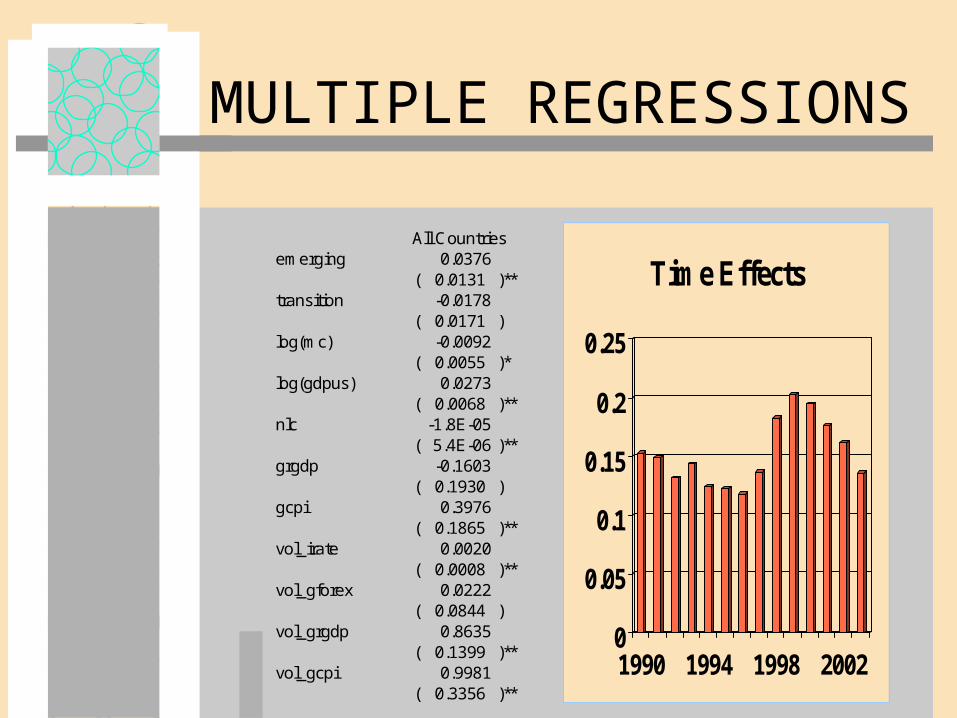
MULTIPLE REGRESSIONS

0

0.05

0.1

0.15

0.2

0.25

1990 1994 1998 2002

Time EffectsAll Countries

emerging 0.0376( 0.0131 )**

transition -0.0178( 0.0171 )

log(mc) -0.0092( 0.0055 )*

log(gdpus) 0.0273( 0.0068 )**

nlc -1.8E-05( 5.4E-06 )**

grgdp -0.1603( 0.1930 )

gcpi 0.3976( 0.1865 )**

vol_irate 0.0020( 0.0008 )**

vol_gforex 0.0222( 0.0844 )

vol_grgdp 0.8635( 0.1399 )**

vol_gcpi 0.9981( 0.3356 )**

IMPLICATIONSIMPLICATIONS

Unconditional volatility varies over Unconditional volatility varies over time and can be modeledtime and can be modeled

Volatility mean reverts to the level of Volatility mean reverts to the level of unconditional volatilityunconditional volatility

Long run volatility forecasts depend Long run volatility forecasts depend upon macroeconomic and financial upon macroeconomic and financial fundamentalsfundamentals

HIGH FREQUENCY HIGH FREQUENCY VOLATILITYVOLATILITY

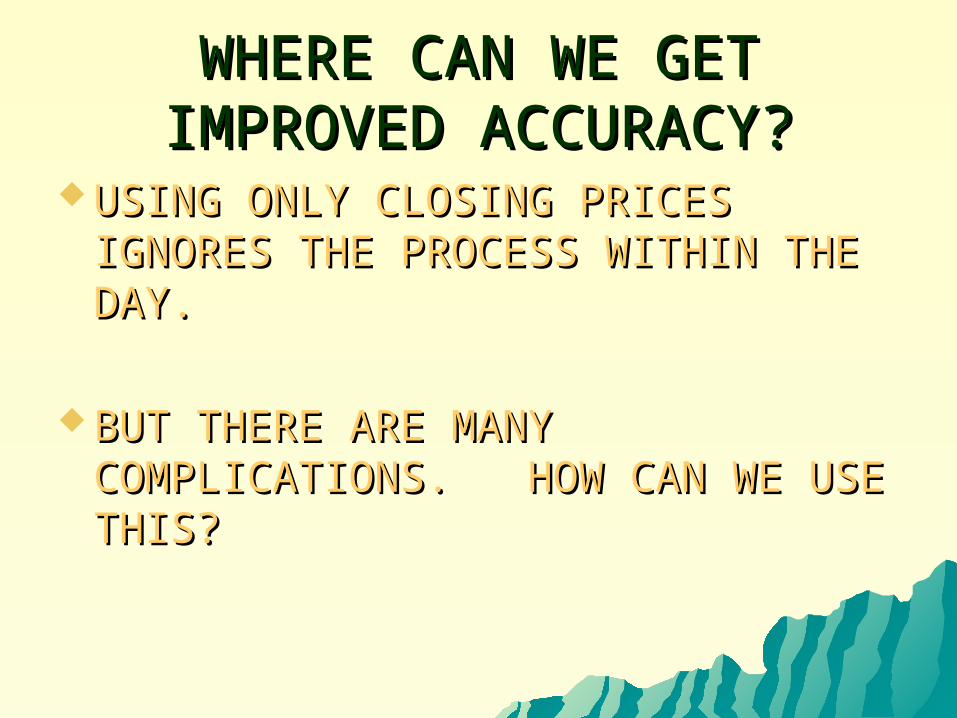
WHERE CAN WE GET WHERE CAN WE GET IMPROVED ACCURACY?IMPROVED ACCURACY?

USING ONLY CLOSING PRICES USING ONLY CLOSING PRICES IGNORES THE PROCESS WITHIN THE IGNORES THE PROCESS WITHIN THE DAY.DAY.

BUT THERE ARE MANY BUT THERE ARE MANY COMPLICATIONS. HOW CAN WE USE COMPLICATIONS. HOW CAN WE USE THIS?THIS?

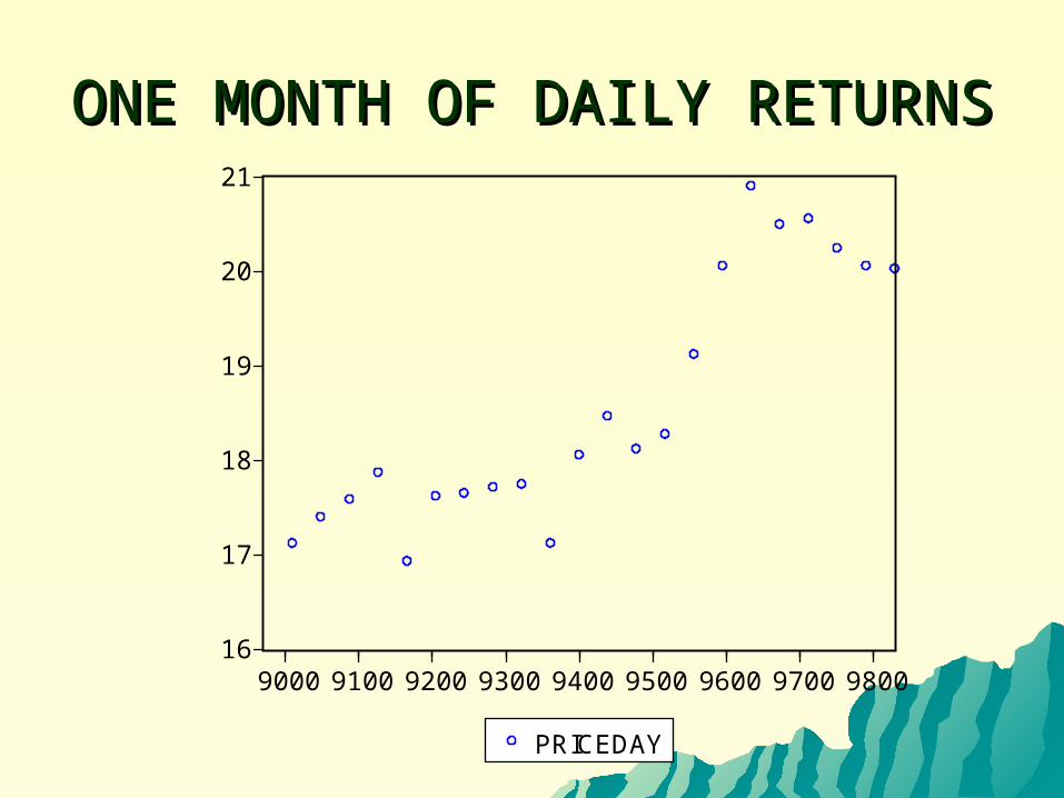
ONE MONTH OF DAILY ONE MONTH OF DAILY RETURNSRETURNS

16

17

18

19

20

21

9000 9100 9200 9300 9400 9500 9600 9700 9800

PRICEDAY

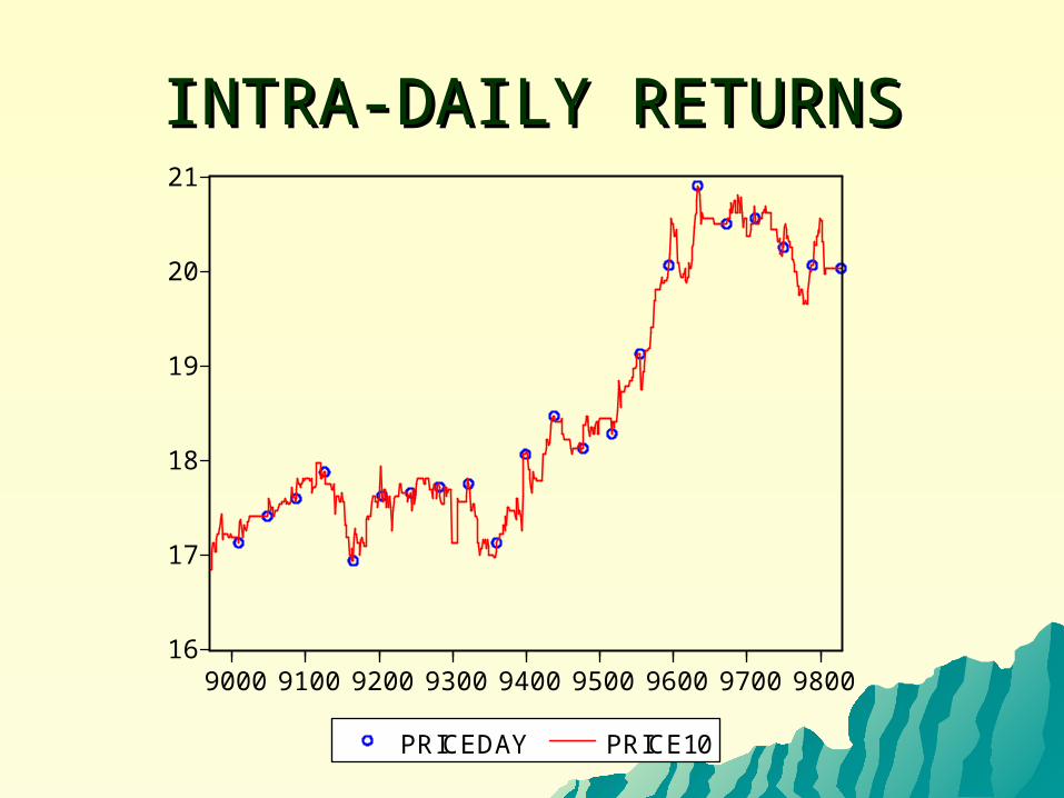
INTRA-DAILY RETURNSINTRA-DAILY RETURNS

16

17

18

19

20

21

9000 9100 9200 9300 9400 9500 9600 9700 9800

PRICEDAY PRICE10

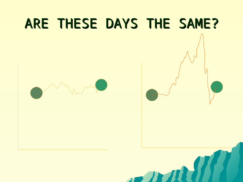
ARE THESE DAYS THE SAME?ARE THESE DAYS THE SAME?

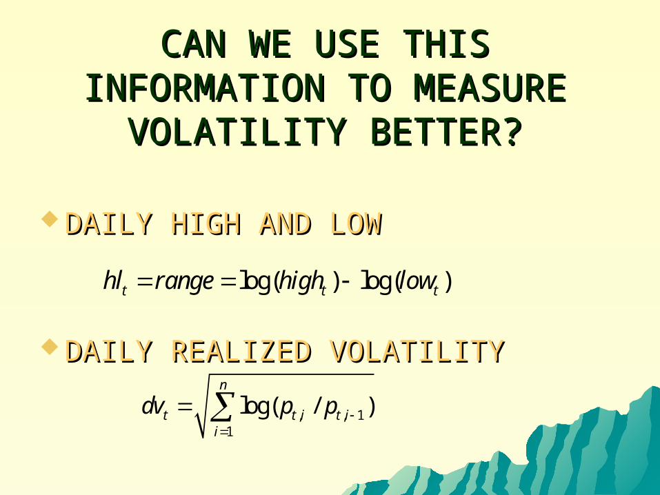
CAN WE USE THIS CAN WE USE THIS INFORMATION TO MEASURE INFORMATION TO MEASURE

VOLATILITY BETTER?VOLATILITY BETTER?

DAILY HIGH AND LOWDAILY HIGH AND LOW

DAILY REALIZED VOLATILITYDAILY REALIZED VOLATILITY

log( ) log( )t t thl range high low

, , 11

log( / )n

t t i t ii

dv p p

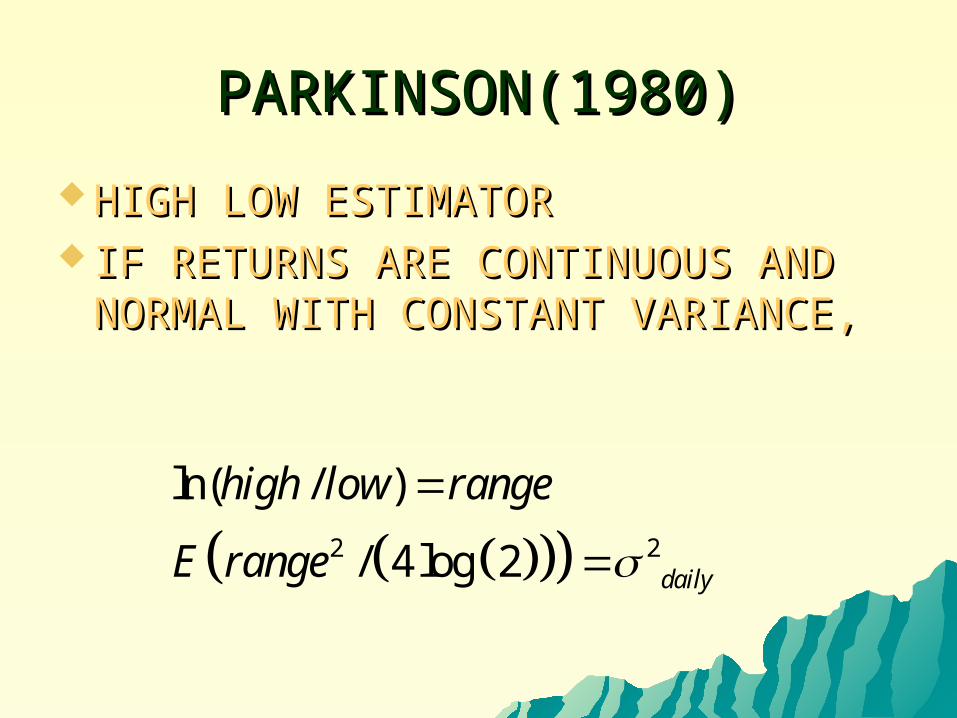
PARKINSON(1980)PARKINSON(1980)

HIGH LOW ESTIMATORHIGH LOW ESTIMATOR IF RETURNS ARE CONTINUOUS AND IF RETURNS ARE CONTINUOUS AND

NORMAL WITH CONSTANT VARIANCE,NORMAL WITH CONSTANT VARIANCE,

2 2

ln( / )

/ 4 log 2 daily

high low range

E range

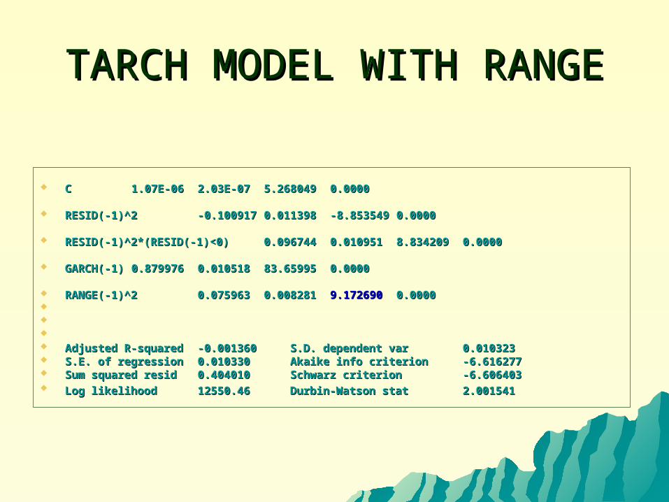
TARCH MODEL WITH RANGETARCH MODEL WITH RANGE

CC 1.07E-061.07E-06 2.03E-072.03E-07 5.2680495.268049 0.00000.0000

RESID(-1)^2RESID(-1)^2 -0.100917-0.100917 0.0113980.011398 -8.853549-8.853549 0.00000.0000

RESID(-1)^2*(RESID(-1)<0)RESID(-1)^2*(RESID(-1)<0) 0.0967440.096744 0.0109510.010951 8.8342098.834209 0.00000.0000

GARCH(-1)GARCH(-1) 0.8799760.879976 0.0105180.010518 83.6599583.65995 0.00000.0000

RANGE(-1)^2RANGE(-1)^2 0.0759630.075963 0.0082810.008281 9.1726909.172690 0.00000.0000

Adjusted R-squaredAdjusted R-squared -0.001360-0.001360     S.D. dependent var    S.D. dependent var 0.0103230.010323 S.E. of regressionS.E. of regression 0.0103300.010330     Akaike info criterion    Akaike info criterion -6.616277-6.616277 Sum squared residSum squared resid 0.4040100.404010     Schwarz criterion    Schwarz criterion -6.606403-6.606403 Log likelihoodLog likelihood 12550.4612550.46     Durbin-Watson stat    Durbin-Watson stat 2.0015412.001541

A MULTIPLE INDICATOR MODEL FOR VOLATILITY USING INTRA-DAILY DATA

Robert F. Engle Robert F. Engle Giampiero M. GalloGiampiero M. Gallo

Forthcoming, Journal of Econometrics

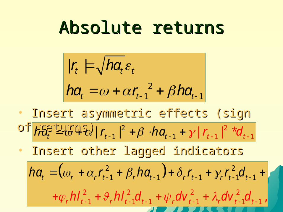
Absolute returnsAbsolute returns

21 1

| |t t t

t t t

r ha

ha r ha

12

1 12

1 | | *| |t t tt tha r ha r d

• Insert asymmetric effects (sign of Insert asymmetric effects (sign of returns)returns)

2 21 1 1

2 2 2 21 1 1

1 1

1 1 1,

t r r t r t r t r

r t r t t r t r t

t

t

t

hl

ha r

hl d dv dv d

ha r r d

• Insert other lagged indicatorsInsert other lagged indicators

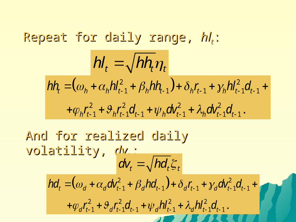
t t thl hh

2 21 1 1 1 1

2 2 2 21 1 1 1 1 1.

t h h t h t h t h t t

h t h t t h t h t t

hh hl hh r hl d

r r d dv dv d

Repeat for daily range, Repeat for daily range, hlhltt::

And for realized daily volatility, And for realized daily volatility, dvdvt t ::

t t tdv hd

2 21 1 1 1 1

2 2 2 21 1 1 1 1 1.

t d d t d t d t d t t

d t d t t d t d t t

hd dv hd r dv d

r r d hl hl d

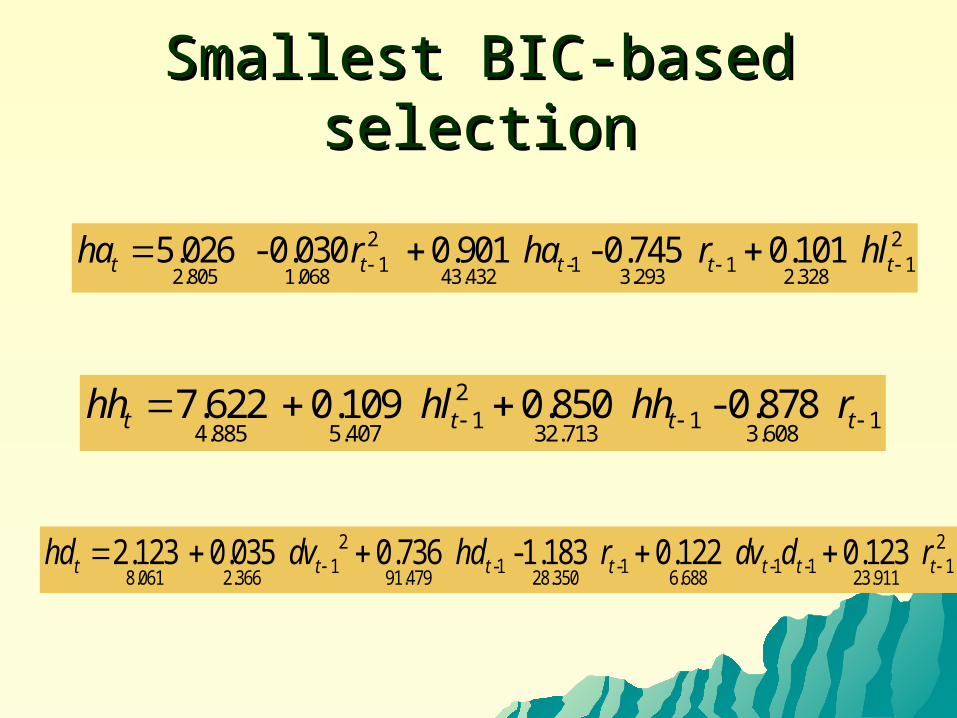
Smallest BIC-based selectionSmallest BIC-based selection

2 21 -1 1 1

2.805 1.068 43.432 3.293 2.3285.026 - 0.030 0.901 - 0.745 0.101t t t t tha r ha r hl

21 1 1

4.885 5.407 32.713 3.6087.622 0.109 0.850 - 0.878t t t thh hl hh r

2 21 -1 -1 -1 -1 1

8.061 2.366 91.479 28.350 6.688 23.9112.123 0.035 0.736 -1.183 0.122 0.123t t t t t t thd dv hd r dv d r

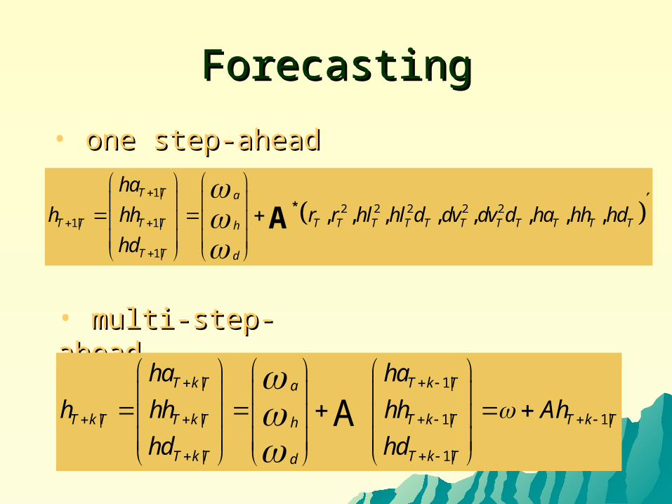
ForecastingForecasting

1|

2 2 2 2 21| 1|

1|

, , , , , , , ,T T a

T T T T T T T T T T T T T T Th

T T d

ha

h hh r r hl hl d dv dv d ha hh hd

hd

*

A

• one step-aheadone step-ahead

• multi-step-multi-step-aheadahead

| 1|

| | 1| 1|

| 1|

AT k T T k Ta

T k T T k T T k T T k Th

T k T T k Td

ha ha

h hh hh Ah

hd hd

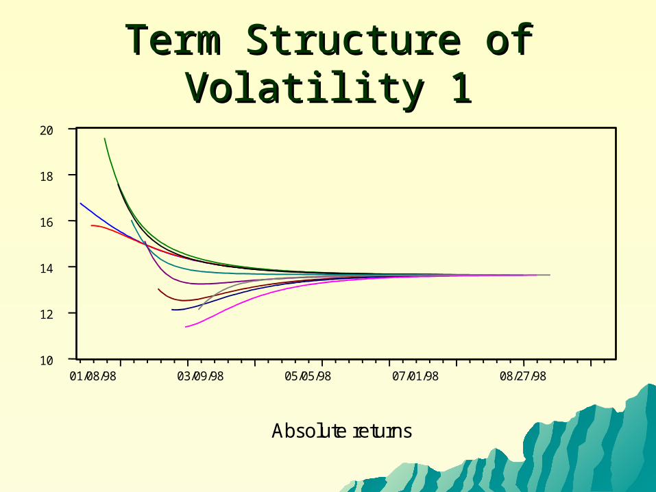
Term Structure of VolatilityTerm Structure of Volatility 1 1

10

12

14

16

18

20

01/08/98 03/09/98 05/05/98 07/01/98 08/27/98

Absolute returns

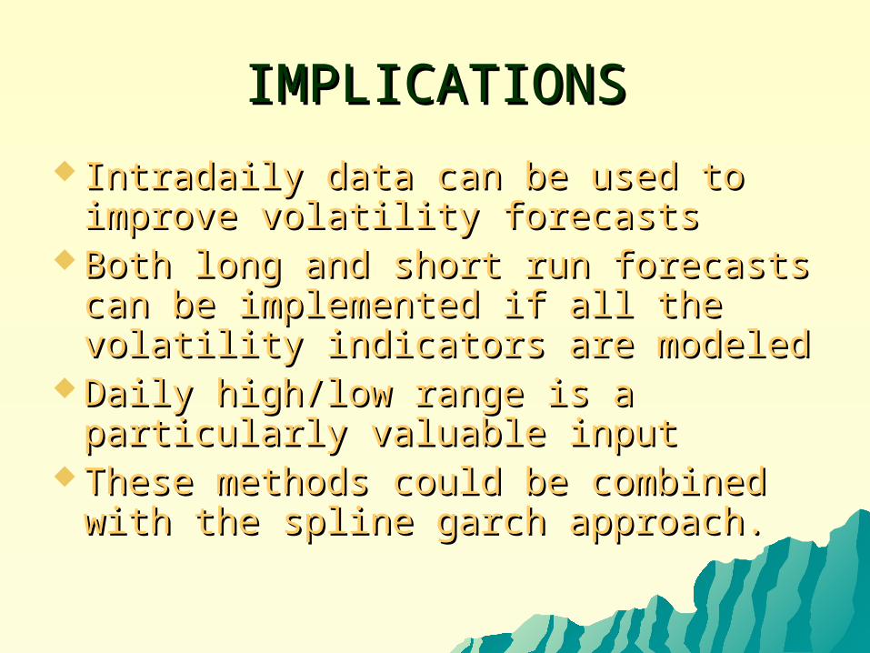
IMPLICATIONSIMPLICATIONS

Intradaily data can be used to Intradaily data can be used to improve volatility forecastsimprove volatility forecasts

Both long and short run forecasts can Both long and short run forecasts can be implemented if all the volatility be implemented if all the volatility indicators are modeledindicators are modeled

Daily high/low range is a particularly Daily high/low range is a particularly valuable inputvaluable input

These methods could be combined These methods could be combined with the spline garch approach.with the spline garch approach.