Embed Size (px)
Citation preview
OPEN ACCESS
Cavity-assisted backaction cooling of mechanicalresonatorsTo cite this article: I Wilson-Rae et al 2008 New J. Phys. 10 095007
View the article online for updates and enhancements.
You may also likeForce sensing based on coherentquantum noise cancellation in a hybridoptomechanical cavity with squeezed-vacuum injectionAli Motazedifard, F Bemani, M H Naderi etal.
-
Mechanical entanglement via detunedparametric amplificationA Szorkovszky, A A Clerk, A C Doherty etal.
-
Large gain quantum-limited qubitmeasurement using a two-mode nonlinearcavityS Khan, R Vijay, I Siddiqi et al.
-
This content was downloaded from IP address 39.122.37.166 on 19/03/2022 at 07:13
T h e o p e n – a c c e s s j o u r n a l f o r p h y s i c s
New Journal of Physics
Cavity-assisted backaction cooling ofmechanical resonators
I Wilson-Rae1,3, N Nooshi1, J Dobrindt2, T J Kippenberg2
and W Zwerger1
1 Technische Universität München, D-85748 Garching, Germany2 Max Planck Institut für Quantenoptik, D-85748 Garching, GermanyE-mail: [email protected]
New Journal of Physics 10 (2008) 095007 (19pp)Received 22 April 2008Published 30 September 2008Online at http://www.njp.org/doi:10.1088/1367-2630/10/9/095007
Abstract. We analyze the quantum regime of the dynamical backactioncooling of a mechanical resonator assisted by a driven harmonic oscillator(cavity). Our treatment applies to both optomechanical and electromechanicalrealizations and includes the effect of thermal noise in the driven oscillator. Inthe perturbative case, we derive the corresponding motional master equationusing the Nakajima–Zwanzig formalism and calculate the correspondingoutput spectrum for the optomechanical case. Then we analyze the strongoptomechanical coupling regime in the limit of small cavity linewidth. Finally,we consider the steady state covariance matrix of the two coupled oscillatorsfor arbitrary input power and obtain an analytical expression for the finalmechanical occupancy. This is used to optimize the drive’s detuning and inputpower for an experimentally relevant range of parameters that includes theresolved-sideband-limit ground state cooling regime.
3 Author to whom any correspondence should be addressed.
New Journal of Physics 10 (2008) 0950071367-2630/08/095007+19$30.00 © IOP Publishing Ltd and Deutsche Physikalische Gesellschaft
2
Contents
1. Introduction 22. Optomechanical master equation 43. Perturbative cooling 6
3.1. Master equation for mechanical motion . . . . . . . . . . . . . . . . . . . . . 63.2. Output power spectrum and temperature measurement . . . . . . . . . . . . . 9
4. Linearized theory for coupled optomechanical modes 124.1. Small cavity linewidth limit κ � gm . . . . . . . . . . . . . . . . . . . . . . . 124.2. Final occupancy for arbitrary ratio gm/κ and optimal parameters . . . . . . . . 14
5. Conclusion 17Acknowledgment 17References 18
1. Introduction
Recent progress in the emerging fields of nanoelectromechanical [1, 2] and optomechanicalsystems [3, 4] promises to enable quantum-limited control of a single macroscopic mechanicaldegree-of-freedom [5, 6]. This is relevant in the context of high precision measurements [7]–[11]like single spin magnetic resonance force microscopy (MRFM) [12, 13] and for fundamentalstudies of the quantum to classical transition [14]–[16]. A paradigmatic goal which has triggereda surge of activity is to prepare the eigenmode associated with an ultra long-lived mechanicalresonance (angular frequency ωm and Q-value Qm) in its quantum ground state with highfidelity [17]–[29]. The considerable difficulty to achieve the desired combination kBT � hωm,Qm � 1 with state of the art micro-fabrication and cryogenic techniques [2] has naturallymotivated ideas to use cooling schemes analogous to the laser-cooling of atoms [30]–[33].
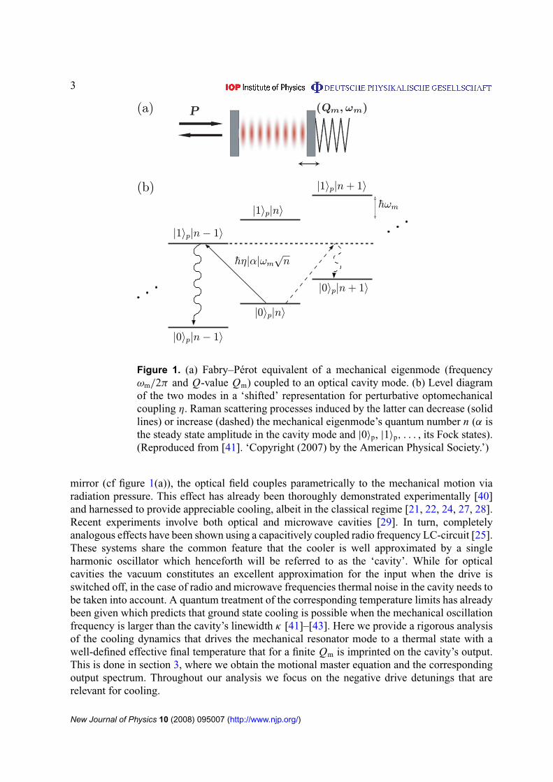
In these schemes, the mechanical resonator’s displacement is coupled parametrically toan auxiliary high-frequency bosonic or fermionic resonator (pseudospin) that can act as a‘cooler’ [34]. To drive the latter while monitoring its output allows detection of the mechanicaldisplacement. Naturally there is a backaction force associated with this measurement process[35]–[37]. Due to the dissipative dynamics of the cooler for a negative detuning of the drive thisforce becomes anti-correlated with the Brownian motion resulting in net cooling. In turn thequantum fluctuations of the cooler—which in the atomic laser cooling manifest in the inherentstochastic nature of the spontaneous photon emissions—result in a quantum noise spectrum forthis backaction force that sets a fundamental lower bound for the final temperature [31, 32]. Thusthe structured reservoir afforded by the driven cooler and its environment provides an effectivethermal bath for the mechanical resonator. The concomitant absorptions of motional quanta(cooling) correspond to Raman scattering processes in which a drive quanta is up converted,whereas emission events (heating) are associated with Raman processes in which a drive quantais down converted (cf figure 1(b)).
A host of concrete realizations of the above generic scenario have been discussed in theliterature. These range from electronic or electrical devices where the cooler is provided by a(superconducting) single electron transistor [20], a Cooper-pair box [38], an LC-circuit [3],or a quantum dot [39]; to optomechanical systems where this role is played by an opticalcavity mode [4]. In the latter systems, which are equivalent to a Fabry–Pérot with a moving
New Journal of Physics 10 (2008) 095007 (http://www.njp.org/)
3
(a)
(b)
|1〉p|n− 1〉|1〉p|n〉
|1〉p|n+ 1〉
|0〉p|n− 1〉
|0〉p|n〉
|0〉p|n+ 1〉
hη|α|ωm√n
hωm
Figure 1. (a) Fabry–Pérot equivalent of a mechanical eigenmode (frequencyωm/2π and Q-value Qm) coupled to an optical cavity mode. (b) Level diagramof the two modes in a ‘shifted’ representation for perturbative optomechanicalcoupling η. Raman scattering processes induced by the latter can decrease (solidlines) or increase (dashed) the mechanical eigenmode’s quantum number n (α isthe steady state amplitude in the cavity mode and |0〉p, |1〉p, . . . , its Fock states).(Reproduced from [41]. ‘Copyright (2007) by the American Physical Society.’)
mirror (cf figure 1(a)), the optical field couples parametrically to the mechanical motion viaradiation pressure. This effect has already been thoroughly demonstrated experimentally [40]and harnessed to provide appreciable cooling, albeit in the classical regime [21, 22, 24, 27, 28].Recent experiments involve both optical and microwave cavities [29]. In turn, completelyanalogous effects have been shown using a capacitively coupled radio frequency LC-circuit [25].These systems share the common feature that the cooler is well approximated by a singleharmonic oscillator which henceforth will be referred to as the ‘cavity’. While for opticalcavities the vacuum constitutes an excellent approximation for the input when the drive isswitched off, in the case of radio and microwave frequencies thermal noise in the cavity needs tobe taken into account. A quantum treatment of the corresponding temperature limits has alreadybeen given which predicts that ground state cooling is possible when the mechanical oscillationfrequency is larger than the cavity’s linewidth κ [41]–[43]. Here we provide a rigorous analysisof the cooling dynamics that drives the mechanical resonator mode to a thermal state with awell-defined effective final temperature that for a finite Qm is imprinted on the cavity’s output.This is done in section 3, where we obtain the motional master equation and the correspondingoutput spectrum. Throughout our analysis we focus on the negative drive detunings that arerelevant for cooling.
New Journal of Physics 10 (2008) 095007 (http://www.njp.org/)
4
The above picture is only valid when the optomechanical coupling defined by gm ≡
2η|α|ωm is perturbative (here |α| is the steady state amplitude in the cavity and η characterizesthe intrinsic nonlinearity). Thus, it breaks down when the resulting cooling rate becomescomparable to the cavity linewidth κ or to the mechanical oscillation frequency ωm [42]. Inthe Doppler limit ωm � κ [31, 32], the system then either becomes unstable [44] (cf belowequation (58)) or settles into a regime where back-action effects are mainly diffusive withno appreciable cooling. On the other hand, in the resolved sideband limit κ � ωm as theoptomechanical coupling exceeds the cavity linewidth the system enters into a strong couplingregime in which the motion hybridizes with the cavity fluctuations. The ensuing optomechanicalnormal modes are then cooled simultaneously. This phenomenon is analyzed in section 4 in thelimit of small cavity linewidth where we find that the dynamics of each of the normal modescan be described by a master equation analogous to the one valid in the perturbative regimewith a cooling rate given by half the cavity linewidth. Finally, in the same section we derivean analytical expression for the final (steady state) average mechanical occupancy (phononnumber) valid for arbitrary optomechanical coupling and use it to optimize the parameters ofthe drive.
2. Optomechanical master equation
In optomechanical systems (and their electromechanical analogues), the cavity resonantfrequency ωp depends inversely on a characteristic length that is modified by the mechanicalresonator’s displacement. The fact that ωp � ωm allows for an adiabatic treatment of this effectwhich results in the aforementioned parametric coupling. In general the leading contributionto the latter is linear in the mechanical displacement—but situations in which it is insteadquadratic can be readily engineered [27, 43]. The desired cooling dynamics is induced bya slightly detuned electromagnetic drive (angular frequency ωL), which for optomechanicalsystems corresponds to an incident laser and in the electromechanical case is afforded by asuitable external ac voltage. Thus the Hamiltonian describing the coupled system (in a rotatingframe at ωL) is given by [45]
H ′= −h1′
La†pap + hηωma†
pap
(am + a†
m
)+ h
�
2
(ap + a†
p
)+ hωma†
mam. (1)
Here ap (am) is the annihilation operator for the electromagnetic (mechanical) oscillator and1′
L is the detuning of the drive from ωp. Here we have defined � ≡ 2√
Pκex/hωL, where Pis the input power of the drive and κex is the cavity decay rate into the associated outgoingelectromagnetic modes. The dimensionless parameter η, characterizing the nonlinear couplingbetween the cavity and the mechanical resonator, is given by η = (ωp/ωm)(x0/L) where x0 isthe zero point motion of the mechanical resonator mode and the characteristic length L dependson the physical realization. In the optomechanical case, it corresponds to an effective opticalcavity length while for electromechanical realizations [25] L = 2dC tot/Cc, where Cc ∝ 1/d isthe dynamical capacitance, d is the distance between the corresponding electrodes and Ctot isthe total capacitance.
We treat the losses induced by the electromagnetic and mechanical baths within therotating wave Born–Markov approximation using the standard Lindblad form Liouvillians [46].It is important to note that the validity of a rotating wave approximation (RWA) in theenvironmental coupling responsible for the mechanical losses only amounts to Qm � 1
New Journal of Physics 10 (2008) 095007 (http://www.njp.org/)
5
provided the optomechanical coupling is weak enough that there is no appreciable mixingbetween the annihilation and creation operators of the modes (cf section 4). Clearly if the latter isnot satisfied the usual RWA will result in the unwarranted neglection of resonant terms. This canbe borne out by comparing the corresponding displacement spectra and results in the conditionη|α|ωm � max{
√ωmκ, ωm}. Henceforth, we focus on parameters that satisfy it which include
the most relevant regimes for cooling and ensure that the system has a stable steady state for therelevant detunings [44, 47]. Thus the evolution for the density matrix of the resonator–cavitysystem reads
ρ = −i
h[H ′, ρ] +
κ
2n(ωp)
(2a†
pρap − apa†pρ − ρapa†
p
)+
κ
2[n(ωp) + 1]
(2apρa†
p − a†papρ − ρa†
pap
)+γm
2n(ωm)
(2a†
mρam − ama†mρ − ρama†
m
)+γm
2[n(ωm) + 1]
(2amρa†
m − a†mamρ − ρa†
mam
). (2)
The total cavity decay rate κ has two contributions: (i) the rate at which photons are lostfrom the open port (where the driving field comes in) given by κex and (ii) the ‘internal loss’rate κ − κex due to the other losses of the electromagnetic resonator (i.e. absorption insidethe dielectric, scattering into other modes, etc). Naturally the thermal noise is determined bythe Bose number n(ω). At room temperature and for optical frequencies n(ωp) is negligible,however for the much lower radio and microwave frequencies characterizing electromechanicalsetups this quantity can be comparable to the final mechanical occupancies achieved. Similarlyγm = ωm/Qm is the mechanical resonator’s natural linewidth and n(ωm) its mean occupationnumber at thermal equilibrium (i.e. in the absence of the drive). Mechanical damping, whichplays a ubiquitous role in determining the temperature limits (cf equation (54)), is usuallydescribed in a phenomenological manner by introducing an Ohmic damping force [48]∼ −γm Xm (where Xm ≡ (am + a†
m)/√
2). A microscopic derivation of mechanical dissipationdue to phonon-tunneling into the supports of the mechanical resonator has recently been givenby Wilson-Rae in [49], which identifies conditions under which such an Ohmic model is indeedjustified and gives geometric upper bounds on the associated mechanical Q-values Qm.
To study the cooling process it proves useful to apply a canonical transformation of theform ap → ap + α, am → am + β with the amplitudes α, β chosen so that the linear terms in thetransformed Liouvillian cancel out. This condition leads to the following coupled equations forthe amplitudes
� −
(1′
L + iκ
2
)α + ηωmα(β + β∗) = 0,(
ωm − iγm
2
)β + ηωm|α|
2= 0.
(3)
We assume η � 1 and that the mechanical dissipation rate γm is much smaller than ωm. Tolowest order in the small parameters η and 1/Qm we obtain α ≈ �/(21′
L + iκ) and β ≈ −η|α|2.
Here |α|2 is the steady state occupancy of the cavity and β is the static shift of the mechanical
amplitude due to the radiation pressure. The normal coordinates after the transformationare shifted so that the new amplitudes correspond to the deviation from the steady stateequilibrium position. This transformation leaves the dissipative part of the Liouvillian invariantand transforms the Hamiltonian into:
H = −h1La†pap + hωma†
mam + hηωm
(a†
pap + α∗ap + αa†p
) (am + a†
m
), (4)
New Journal of Physics 10 (2008) 095007 (http://www.njp.org/)
6
where we have introduced the effective detuning 1′
L + 2η2|α|
2ωm → 1L. It is interesting tonote that if the bosonic cooler is replaced by a fermionic one so that ap → σ− we obtain aHamiltonian that resembles the one describing a trapped ion in the Lamb–Dicke regime. Asa result for perturbative η (as analyzed in the next section) the cooling cycle (cf figure 1(b))becomes analogous to the Lamb–Dicke regime of atomic laser-cooling [41].
3. Perturbative cooling
3.1. Master equation for mechanical motion
We first focus on the regime in which the input laser power P is low enough so that thetimescales over which the populations of the mechanical resonator’s Fock states evolve (leadingto cooling or heating) are much slower than those associated with the losses of the cavity andwith the free mechanical frequency. As will become clear below this requires η2
|α|2� (κ/ωm)2.
Here we also assume [n(ωm) + 1]γm � κ , ωm which must hold to allow for appreciablecooling, and η2
� 1 (in optomechanical realizations η . 10−4). Hence the electromagneticdegrees of freedom can be treated as a structured environment that affects the mechanical motionperturbatively. Along these lines the latter can be described by a Markovian master equation forits reduced density matrix [46].
To derive it we take the optomechanical master equation in the shifted representation,transform to an interaction picture for the resonator mode and adiabatically eliminate the cavityusing the Nakajima–Zwanzig formalism [46, 50, 51]. The optomechanical coupling and themechanical losses are treated perturbatively. We define the projection
Pρ = Trp{ρ} ⊗ ρ(th)p , Q≡ 11 −P, (5)
with
ρ(th)p =
1
np + 1
∞∑n=0
[np
np + 1
]n
|n〉〈n|p, (6)
where np ≡ n(ωp) is the Bose number, and introduce the formal parameter ζ such that
L(t) = ζ 2L0 + ζL1(ζ2t) +L2, (7)
with
L0ρ ≡ i[1La†
pap, ρ]
+κ
2n(ωp)
[2a†
pρap − apa†pρ − ρapa†
p
]+
κ
2[n(ωp) + 1]
[2apρa†
p − a†papρ − ρa†
pap
], (8)
L1(ζ2t) ≡ eiωmζ 2tL(+)
1 + e−iωmζ 2tL(−)
1 , (9)
L(+)
1 ρ ≡ −i[ηωm
[a†
pap + α∗ap + αa†p
]a†
m, ρ], (10)
L(−)
1 ρ ≡ −i[ηωm
[a†
pap + α∗ap + αa†p
]am, ρ
], (11)
L2 ≡γm
2n(ωm)
(2a†
mρam − ama†mρ − ρama†
m
)+
γm
2[n(ωm) + 1]
(2amρa†
m − a†mamρ − ρa†
mam
). (12)
New Journal of Physics 10 (2008) 095007 (http://www.njp.org/)
7
We note that Pρ is a stationary state of L0 for any ρ implying that L0P = 0, while PL0 = 0follows from trace preservation, so that we have
QL0Q= L0, PL0P =QL0P = PL0Q= 0. (13)
As will emerge from our derivation the basic idea is that the rates for cooling and heating setthe relevant timescale (zeroth order in 1/ζ ) which is widely separated from the mechanicaloscillation period 2π/ωm and the cavity lifetime 1/κ (order 1/ζ 2). In fact, the asymptoticexpansion for ζ → ∞ pursued below amounts to a controlled expansion in the ratio between thefast and the slow timescales. Given that we are interested in the behavior as t → ∞, the initialcondition is immaterial and we choose for simplicity one in the P-manifold so that Qρ0 = 0.Subsequently, by explicitly integrating the differential equation for the irrelevant part Qρ, weobtain a closed equation for the relevant part Pρ:
Pρ = PL(t)Pρ +PL(t)∫ t
0dτT+
[e∫ t
0 dτ ′QL(τ ′)Q]T−
[e−
∫ τ
0 dτ ′′QL(τ ′′)Q]L(τ )Pρ(τ), (14)
where T+ (T−) is the time-ordering (anti-time-ordering) operator. For the purpose of analyzingthe asymptotic limit ζ → ∞ of equation (14) we have
T+
[e∫ t
0 dτ ′QL(τ ′)Q]T−
[e−
∫ τ
0 dτ ′′QL(τ ′′)Q]
= eζ 2QL0Q(t−τ)
[11 + O
(1
ζ
)], (15)
which can be understood considering the corresponding Laplace transforms. Substitution ofequations (13) and (15) into (14) and the change of variables τ ′
= ζ 2(t − τ) then yields
Pρ=P[ζL1(ζ
2t) +L2
]Pρ +PL1(ζ
2t)Q∫ ζ 2t
0dτ ′eL0τ
′QL1(ζ2t − τ ′)Pρ(t − τ ′/ζ 2) + · · · . (16)
Here we have also used Q2=Q, P2
= P and PL2 = L2P . The leading order in 1/ζ of theevolution over the aforementioned relevant timescale will be determined by the limit as ζ → ∞
of the Laplace transform of the above. In the time domain all the fast rotating terms (frequenciesof order ζ 2ωm) drop out and equation (16) reduces to
Pρ = PL2Pρ +[PL(+)
1 Q∫
∞
0dτ ′e(iωm+L0)τ
′QL(−)
1 Pρ + h.c.]
. (17)
We note that as P = limt→∞ eL0t we have
L0ρ = 0 ⇒ Qρ = 0. (18)
It follows that the restriction of L0 to the Q-manifold has only eigenvalues with negative realparts which allows us to establish
Q∫
∞
0dτ ′e(iωm+L0)τ
′Q=Q (−iωm −L0)−1Q. (19)
We focus on the parameter regime where |α|2� np. The behavior of the cavity correlations
that determine the second term in equation (17) implies that in this regime contributions arisingfrom the cubic term in L(±)
1 are negligible compared to those generated by the quadratic term—for np = 0, the contributions of the former are higher order in η. The conditions that warrantthis linearization of L(±)
1 for the case np = 0 will be discussed further in the next subsection.
New Journal of Physics 10 (2008) 095007 (http://www.njp.org/)
8
The restriction of the quadratic term to the P-manifold vanishes and we obtain
Trp
{PL(+)
1 Q∫
∞
0dτ ′e(iωm+L0)τ
′QL(−)
1 Pρ
}≈ −
g2m
2
{G(ωm, np)
[a†
m, amµ]− G∗(−ωm, np)
[a†
m, µam
]}. (20)
Here, we have used equations (5), (10) and (11), and introduced the optomechanical coupling
gm ≡ 2η|α|ωm, (21)
the reduced density matrix for the mechanical mode µ ≡ Trp{ρ}, and the cavity-quadratures’correlations
G(ω, np) =
∫∞
0dτeiωτ Trp
{Xp(0)eL0τ Xp(0)ρ(th)
p
}, (22)
with Xp(0) ≡ (α∗ap + αa†p)/
√2|α|. If we substitute equations (5), (12) and (20) into (17), trace
out the cavity, and rearrange we finally obtain the following master equation:
µ = −i[(ωm + 1m)a†
mam, µ]
+ 12{γm[n(ωm) + 1] + A−(np)}
(2amµa†
m − a†mamµ − µa†
mam
)+1
2 [γmn(ωm) + A+(np)](2a†
mµam − ama†mµ − µama†
m
), (23)
where the cooling (heating) rate A−(np) [A+(np)] and the mechanical frequency shift 1m
induced by the optomechanical coupling are given by
A∓(np) = g2m<{G(±ωm, np)}, (24)
1m =g2
m
2={G(ωm, np) − G(−ωm, np)}. (25)
It is straightforward to calculate the necessary two-time correlations using the quantumregression theorem given the steady state moments:⟨
apa†p
⟩= np + 1,
⟨a†
pap
⟩= np,
⟨apap
⟩= 0 (26)
and that the evolution of the mean amplitude reads
〈ap〉 = (i1L − κ/2) 〈ap〉. (27)
Thus we obtain
G(ω, np) =[G(ω, 0) + G∗(ω, 0)
]np + G(ω, 0) (28)
with
G(ω, 0) =1
−2i(ω + 1L) + κ, (29)
which substituted into equations (24) and (25) leads to
A∓(np) = [A−(0) + A+(0)]np + A∓(0), (30)
1m = g2m
[1L − ωm
4(1L − ωm)2 + κ2+
1L + ωm
4(1L + ωm)2 + κ2
], (31)
where the corresponding rates in the absence of thermal noise in the driven cavity are given by
A∓(0) = g2m
κ
4(1L ± ωm)2 + κ2. (32)
New Journal of Physics 10 (2008) 095007 (http://www.njp.org/)
9
The above can be related to the input power and the frequency of the drive via
gm = 2ηωm
√Pκex
hωL(1′
L2 + κ2/4)
, (33)
1L = 1′
L + 2η2ωmPκex
hωL(1′
L2 + κ2/4)
. (34)
The master equation (23) generalizes the one obtained in [41] by including thermal noisein the cavity input. As shown below, this effect is significant for determining the ultimate limitto which the mechanical resonator can be cooled for ratios ωp/ωm like the ones that characterizeelectromechanical realizations. Equation (23) has as its steady state a thermal state which definesthe effective final temperature to which the mechanical resonator is cooled. The correspondingfinal occupancy reads [0 ≡ A−(0) − A+(0)]:
nf =γm
0 + γmn(ωm) +
0
0 + γm
[(2nf + 1)np + nf
], (35)
where nf is the quantum backaction contribution derived in [41, 42], namely
nf = −(1L + ωm)2
41Lωm. (36)
We note that in the ‘unshifted’ representation there is in addition a coherent shift of theresonator’s normal coordinate so that⟨
a†mam
⟩= nf + η2
[Pκex
hωL(1′
L2 + κ2/4)
]2
. (37)
If we now consider the appreciable cooling limit 0 � γm and minimize with respect to thedetuning we obtain
min{nf} ≈γmκ
√ω2
m + κ2/4
g2mωm
n(ωm) + np +(
np +1
2
)(√1 +
κ2
4ω2m
− 1
), (38)
for the optimal detuning 1optL =
√ω2
m + κ2/4. The first term corresponds to the ‘linear cooling’limited by thermal noise. In turn, the second term shows that the final occupancy is necessarilybounded by the equilibrium thermal occupancy of the cooler. Finally, the last term for np = 0corresponds to the fundamental temperature limit imposed by the quantum backaction whichin the Doppler regime κ � ωm reduces to κ/4ωm, precluding ground state cooling, whereasin the RSB regime κ � ωm it yields κ2/16ω2
m corresponding to occupancies well below unity[41, 42]. We note that for a given κ/ωm <
√32 occupancies below unity are only attainable
within a finite detuning window |1L + 3ωm|6√
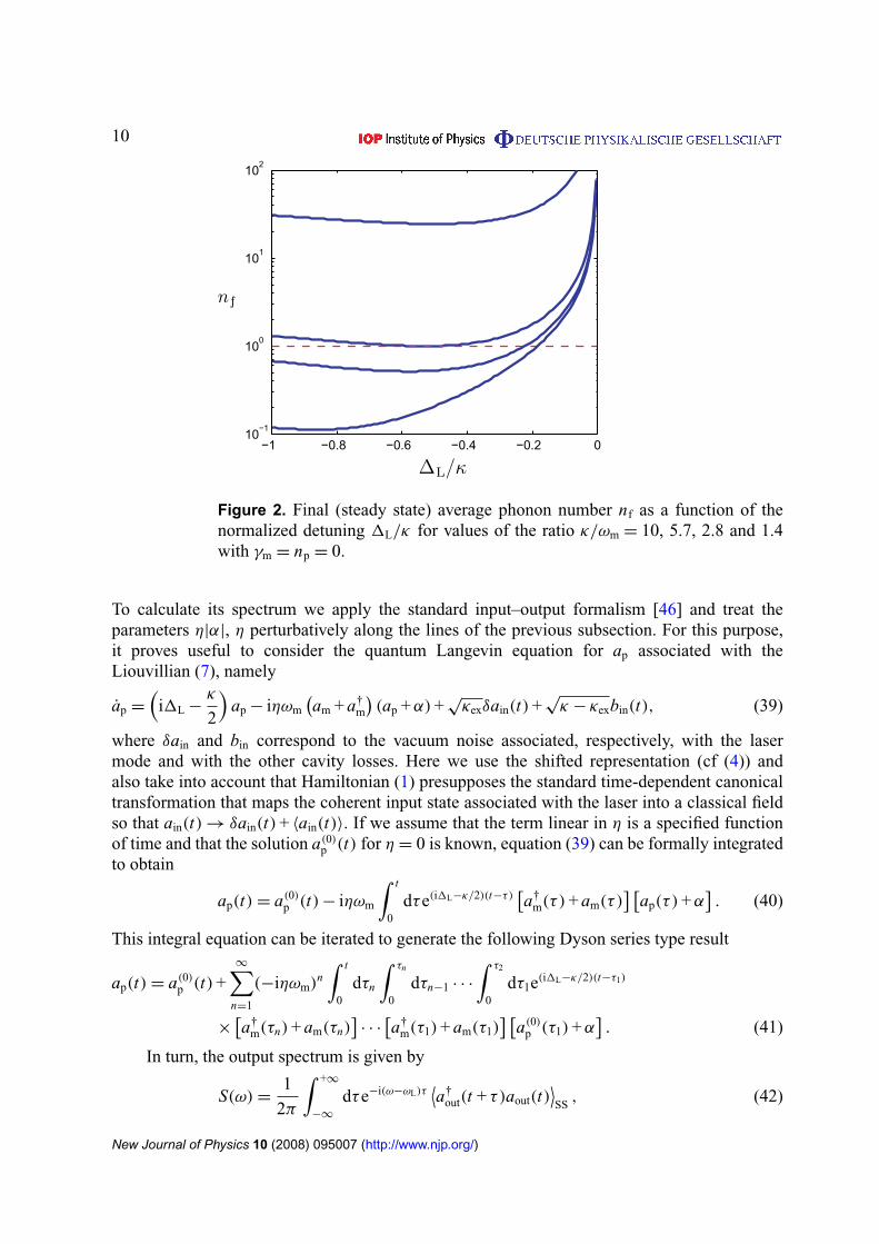
8ω2m − κ2/4, as illustrated in figure 2.
3.2. Output power spectrum and temperature measurement
The spectrum of the cavity output constitutes a crucial observable to understand the back-actioncooling. It allows the cooling cycle to be visualized as a frequency up-conversion process and foroptomechanical realizations it provides an efficient way to measure the final temperature [41].We focus on the latter for which np = 0 and consider the experimentally relevant case inwhich the output is measured in the same modes in which the coherent laser drive is fed [24].
New Journal of Physics 10 (2008) 095007 (http://www.njp.org/)
10
−1 −0.8 −0.6 −0.4 −0.2 010
−1
100
101
102
nf
∆L/κ
Figure 2. Final (steady state) average phonon number nf as a function of thenormalized detuning 1L/κ for values of the ratio κ/ωm = 10, 5.7, 2.8 and 1.4with γm = np = 0.
To calculate its spectrum we apply the standard input–output formalism [46] and treat theparameters η|α|, η perturbatively along the lines of the previous subsection. For this purpose,it proves useful to consider the quantum Langevin equation for ap associated with theLiouvillian (7), namely
ap =
(i1L −
κ
2
)ap − iηωm
(am + a†
m
)(ap + α) +
√κexδain(t) +
√κ − κexbin(t), (39)
where δain and bin correspond to the vacuum noise associated, respectively, with the lasermode and with the other cavity losses. Here we use the shifted representation (cf (4)) andalso take into account that Hamiltonian (1) presupposes the standard time-dependent canonicaltransformation that maps the coherent input state associated with the laser into a classical fieldso that ain(t) → δain(t) + 〈ain(t)〉. If we assume that the term linear in η is a specified functionof time and that the solution a(0)
p (t) for η = 0 is known, equation (39) can be formally integratedto obtain
ap(t) = a(0)p (t) − iηωm
∫ t
0dτe(i1L−κ/2)(t−τ)
[a†
m(τ ) + am(τ )] [
ap(τ ) + α]. (40)
This integral equation can be iterated to generate the following Dyson series type result
ap(t) = a(0)p (t) +
∞∑n=1
(−iηωm)n
∫ t
0dτn
∫ τn
0dτn−1 · · ·
∫ τ2
0dτ1e(i1L−κ/2)(t−τ1)
×[a†
m(τn) + am(τn)]· · ·[a†
m(τ1) + am(τ1)] [
a(0)p (τ1) + α
]. (41)
In turn, the output spectrum is given by
S(ω) =1
2π
∫ +∞
−∞
dτe−i(ω−ωL)τ⟨a†
out(t + τ)aout(t)⟩SS
, (42)
New Journal of Physics 10 (2008) 095007 (http://www.njp.org/)
11
which in the shifted representation reads
S(ω) =1
2π
∫ +∞
−∞
dτe−i(ω−ωL)τ⟨ [
√κexa†
p(t + τ) + δa†in(t + τ) +
√κexα
∗ + 〈ain(0)〉∗
]×
[√
κexap(t) + δain(t) +√
κexα +⟨ain(0)
⟩]⟩SS
. (43)
We now seek the lowest nontrivial order in η. The output aout has a c number part arising fromthe classical drive and the cavity steady state amplitude and an operator part correspondingto the fluctuations. Equation (43) directly implies that terms involving the c numbers onlycontribute to the ‘main line’ ∝ δ(ω − ωL). Furthermore, as in the shifted representation thesteady state of the electromagnetic modes is the vacuum |0〉 it follows from equations (41)and (43) that the contribution of the cross-term with the operator part—which vanishes if thecubic term in equation (4) is omitted—is at most higher order in η and can be neglected relativeto the contribution bilinear in the c numbers. The latter corresponds to the classical reflectioncoefficient that is straightforward to obtain considering the near-resonant scattering into modes(real or fictitious) responsible for the other losses κ − κex. Thus we arrive at
S(ω) ≈P
hωL
[1 −
(κ − κex)κex
12L + κ2/4
]δ(ω − ωL) +
κexg2m
8π
×
∫ +∞
−∞
dτe−i(ω−ωL)τ
⟨∫ t+τ
0dτ ′
1e(−i1L−κ/2)(t+τ−τ ′
1)[a†
m(τ ′
1) + am(τ ′
1)]
×
∫ t
0dτ1e(i1L−κ/2)(t−τ1)
[a†
m(τ1) + am(τ1)]⟩
SS
, (44)
where we have used equation (41) and a(0)p (t)|0〉 = δain|0〉 = 0. Note that the correction is higher
order in η for all frequencies. To calculate the steady state two-time average in equation (44) weadopt (as in the previous subsection) an interaction picture for the resonator mode (i.e. am(t) →
e−iωmtam(t)) and make the substitutions t + τ − τ ′
1 → τ ′
1, t − τ1 → τ1 in the time integrals. In thisrepresentation, the mechanical mode operators evolve slowly compared with 1/κ so that, in linewith our derivation of a Markovian master equation for the mechanical motion, we can factorthem out of the time integrals whose upper limit can be extended to infinity. This Markovianapproximation then yields⟨∫ t+τ
0dτ ′
1e(−i1L−κ/2)(t+τ−τ ′
1)[a†
m(τ ′
1) + am(τ ′
1)] ∫ t
0dτ1e(i1L−κ/2)(t−τ1)
[a†
m(τ1) + am(τ1)]⟩
SS
≈ 4⟨[
G∗(ωm, 0)eiωm(t+τ)a†m(t + τ) + G∗(−ωm, 0) e−iωm(t+τ)am(t + τ)
]×[G(−ωm, 0)eiωmta†
m(t) + G(ωm, 0) e−iωmtam(t)]⟩
SS(45)
where we have used equation (29). The two-time averages of the mechanical mode operatorscan now be calculated from the master equation (23) using the quantum regression theorem.The needed one-time averages satisfy
〈am〉 = −
(i1m +
γm + 0
2
)〈am〉,⟨
a†mam
⟩SS
= nf,⟨ama†
m
⟩SS
= nf + 1,
〈amam〉SS =⟨a†
ma†m
⟩SS
= 0.
(46)
New Journal of Physics 10 (2008) 095007 (http://www.njp.org/)
12
Finally, a straightforward calculation leads from equations (44)–(46), (29) and (32) to thespectrum already given in [41], namely
S(ω) ≈P
hωL
[1 −
(κ − κex)κex
12L + κ2/4
]δ(ω − ωL) +
κex A−nf
κπ
(γeff/2)
(ω − ωL − ωm − 1m)2 + (γ 2eff/4)
+κex A+ (nf + 1)
κπ
(γeff/2)
(ω − ωL + ωm + 1m)2 + (γ 2eff/4)
, (47)
where we have introduced γeff ≡ γm + 0 which is the total dissipation rate for the mechanicalmode in the presence of the drive that determines the linewidths of the motional sidebandspeaked at ωL ± ωm. One should note that the above corresponds to photon rate per unit frequencyand that the weight of the motional sidebands relative to the main line is of order η2(2nf + 1)
(η2 . 10−8 for typical systems). Here unlike the case of atomic laser cooling [31, 32] themechanical dissipation induces an asymmetry in the weights of the sidebands that allows thefinal temperature to be retrieved directly from the steady state. The ‘blue’ sideband weighted byN− =
κexκ
A−nf corresponds to the up-converted photons (anti-Stokes scattering) responsible forthe cooling while the ‘red’ sideband weighted by N+ =
κexκ
A+(nf + 1) corresponds to the down-converted photons (Stokes scattering) that result in heating.
It is interesting to note that the formalism of this section does not presuppose linearizingaround the steady state and neglecting the cubic term in Hamiltonian (4) accordingly, butrather the validity of such treatment emerges from a controlled procedure that would allowthe necessary corrections to be incorporated if the intrinsic nonlinearity η were larger.A straightforward self-consistency criterion is to compare the steady state fluctuation of thecubic term with that of the quadratic one. An heuristic estimate for their ratio can be extractedfrom the total weight of the motional sidebands in equation (47) which together with the analysisin section 3.1 implies that the cubic term can be neglected provided the conditions η2(2nf +1)ω2
m � κ2 and |α|2� η2 are satisfied—for the typical parameters in cooling experiments these
are always met.
4. Linearized theory for coupled optomechanical modes
4.1. Small cavity linewidth limit κ � gm
The treatment in the previous section is only applicable when the cooling rate A− given byequations (30) and (32) is much smaller than κ (note that the heating rate A+ is always boundedby A− for negative detuning). This condition for arbitrary negative detuning results in g2
m � κ2
so that it follows (as expected) that the motional master equation is only warranted for smallenough optomechanical coupling. In the Doppler regime [31, 32], κ � ωm, when this is violatedthe aforementioned condition gm � max{
√ωmκ, ωm} underpinning the RWA for the mechanical
losses will also fail. In contrast, in the resolved sideband regime (RSB) relevant for ground statecooling, κ � ωm implies that there is a wide parameter range of interest in which equation (2)remains valid while equation (23) fails. Here we consider this RSB regime beyond perturbativeoptomechanical coupling. As gm becomes comparable to κ it becomes necessary to follow thecoupled dynamics of both modes as described by equation (2) which for gm > κ/2 exhibitsnormal mode splitting. Though for a Gaussian initial condition the approach to the steady stateis always amenable to a straightforward description, in the intermediate regime gm ∼ κ there willbe no simple analog of equation (23) that allows the cooling process to be visualized in terms
New Journal of Physics 10 (2008) 095007 (http://www.njp.org/)
13
of phonon jumps. In turn, deep in the strong coupling regime but away from the instability [42],i.e. for κ � gm � ωm, the dynamics can be described by two decoupled master equations forthe optomechanical normal modes analogous to equation (23).
Within the latter parameter range it is permissible to start from a Hamiltoniandescription including the optomechanical coupling and treat the losses (as described by γm,κ) perturbatively. We focus on the ‘resonant case’ −1L = ωm—which in the RSB regimecan be shown to be optimal for minimizing the final occupancy—and consider the canonicaltransformation that diagonalizes Hamiltonian (4) for η = 0 with gm 6= 0 (after performing theconvenient rotation ap → (α/|α|)ap). The latter is given by
am/p =1
2√
2
[(√ωm
ω++√
ω+
ωm
)a+ ±
(√ωm
ω−
+√
ω−
ωm
)a−
+(√
ωm
ω+−
√ω+
ωm
)a†
+ ±
(√ωm
ω−
−
√ω−
ωm
)a†
−
], (48)
where the eigenfrequencies of the normal modes read
ω± = ωm(1 ± gm/ωm)1/2. (49)
If we now consider the expansion of the above in the small parameter gm/ωm the zeroth orderof equation (49) yields a splitting given by gm while equation (48) reduces to the transformationthat diagonalizes the rotating wave part of Hamiltonian (4)—that results from neglecting theterms that involve amap and a†
ma†p . The latter transformation does not mix the annihilation
and creation operators. For small but finite gm/ωm there will be small admixtures that for thepurpose of analyzing the cooling dynamics will only be relevant insofar as they give rise toqualitatively new terms in the dissipative part of the Liouvillian—otherwise they can be shownto result in contributions of relative order (gm/ωm)2 for all values of the other parameters. Hencewe have
am/p ≈1
√2
a+ ±1
√2
a− −gm
4√
2ωm
a†+ ±
gm
4√
2ωm
a†−. (50)
To proceed we: (i) apply the transformation given by equation (48) to the masterequation (2), (ii) transform the result to an interaction picture with respect to the (now diagonal)Hamiltonian, (iii) neglect all the resulting fast rotating terms which are ∝e±2iωmt or ∝e±igmt
(up to corrections higher order in gm/ωm), and (iv) expand to lowest order in gm/ωm followingthe aforementioned ‘qualitative’ criterion. Naturally (iii) relies on the small cavity linewidthcondition κ � gm. Thus we obtain
ρ =
∑ξ=±
[γm
4n(ωm) +
κ
4n(ωp) +
κg2m
64 ω2m
] (2a†
ξρaξ − aξa†ξρ − ρaξa†
ξ
)+{γm
4[n(ωm) + 1] +
κ
4[n(ωp) + 1]
} (2aξρa†
ξ − a†ξ aξρ − ρa†
ξ aξ
). (51)
The only corrections in (gm/ωm)2 appear in the first term and correspond to the ‘high powerlimit’ of the heating induced by the quantum backaction of the cavity. Analogous heating terms∝ γm are neglected given that they are comparable to corrections to the RWA treatment of themechanical dissipation. It follows from equation (51) that the losses do not couple the normal
New Journal of Physics 10 (2008) 095007 (http://www.njp.org/)
14
modes (annihilation operators a±) so that the steady state is given by the tensor product ofthermal states for each of them characterized by⟨
a†±
a†±
⟩SS
=γmn(ωm) + κn(ωp) + (κg2
m/16ω2m)
γm + κ, (52)
(where we neglect higher order terms in gm/ωm) to which the average occupancies convergewith a cooling rate (κ + γm)/2. Hence equations (50) and (52) finally yield
nf ≈γmn(ωm) + κn(ωp) + (κg2
m/16 ω2m)
γm + κ+
g2m
16 ω2m
≈γmn(ωm)
κ+ np +
g2m
8ω2m
, (53)
where the corrections are higher order in the small parameters (gm/ωm)2 and γm/κ . Thefirst term corresponds to the heating associated with the mechanical dissipation and can beidentified with the corresponding term in equation (35) showing a saturation of the usual linearcooling law. Similarly, the second and third terms can be identified with the correspondingcontributions in equation (35) arising from the thermal noise in the cavity and the quantumbackaction. Thus ground state cooling requires kBT/hQm � κ � ωm and ωp < kBT/h. We notethat equations (50) and (52) imply that 〈a2
m〉SS = 0 so that the reduced state for the motion is alsothermal in the small κ limit.
If we now compare equations (38) and (53) and consider minimizing them with respect togm within their respective ranges of validity, heuristic considerations imply that the followingformula should always constitute a lower bound for the final mechanical occupancy optimizedwith respect to the parameters of the drive
nTL =γmn(ωm)
κ+ np +
1
2
(√1 +
κ2
4ω2m
− 1
). (54)
This will be borne out quantitatively in section 4.2 by comparing with the results of a treatmentthat is exact within the linearized theory.
4.2. Final occupancy for arbitrary ratio gm/κ and optimal parameters
The approximate expressions (35) and (53) for the final mechanical occupancy that we havederived in the limits gm � κ and gm � κ provide a basic understanding of the requirements forground state cooling and the expected order of magnitude for the optimum. Notwithstandingthey have the drawback that they fail to settle which is the optimal input power as minimizationwith respect to gm shifts this variable away from the domain where they are valid. In addition,given the experimental progress towards achieving ultra-cold states in these systems, it is clearthat precise quantitative predictions for the steady state that results from a given input are highlydesirable. To this effect we complement the above analysis by deriving an analytical expressionfor nf valid for arbitrary values of the ratio gm/κ . The optomechanical master equation (2)directly implies that, when the cubic nonlinearity in Hamiltonian (4) is neglected, the timeevolution for the ten independent second-order moments that determine the covariance matrix
New Journal of Physics 10 (2008) 095007 (http://www.njp.org/)
15
is given by a linear system of ordinary differential equations. This is determined by
d
dt
⟨a†
mam
⟩= −γm
⟨a†
mam
⟩+ γmn(ωm) − i
gm
2
⟨(a†
p + ap
) (a†
m − am
)⟩,
d
dt
⟨apam
⟩= −
(κ
2+
γm
2− i1L + iωm
) ⟨apam
⟩− i
gm
2
(1 +
⟨a†
mam
⟩+⟨a2
m
⟩+⟨a†
pap
⟩+⟨a2
p
⟩),
d
dt
⟨apa†
m
⟩= −
(κ
2+
γm
2− i1L − iωm
) ⟨apa†
m
⟩− i
gm
2
(⟨a†
mam
⟩+⟨a2
m
⟩−⟨a†
pap
⟩−⟨a2
p
⟩),
d
dt
⟨a†
pap
⟩= −κ
⟨a†
pap
⟩− i
gm
2
⟨(a†
p − ap
) (a†
m + am
)⟩+ κn(ωp),
d
dt
⟨a2
m
⟩= − (γm + 2iωm)
⟨a2
m
⟩− igm
⟨(a†
p + ap
)am
⟩,
d
dt
⟨a2
p
⟩= − (κ − 2i1L)
⟨a2
p
⟩− igm
⟨(a†
m + am
)ap
⟩,
(55)
and their Hermitian conjugates. The exact solution for the linear system of equations that resultsfor the steady state covariance matrix then yields an analytical formula for the final occupancyof the mechanical resonator that is a sum of three independent contributions
nf = n(m)
f + n(p)
f + n(0)
f . (56)
Here n(m)
f and n(p)
f arise, respectively, from the mechanical dissipation and the thermal noise inthe cavity input, and n(0)
f corresponds to the heating induced by the quantum backaction exertedby the cavity. The expressions for these different contributions are rather unwieldy for arbitrarymechanical dissipation γm, but it is simple to realize that for appreciable cooling nf � n(ωm) tobe possible the conditions γm � κ , gm, ωm are needed. Hence, in this regime of interest, a goodapproximation for nf is obtained if one takes γm → 0 keeping γmn(ωm) finite. In this limit weobtain
n(0)
f = −1
4ωm1L
[(ωm + 1L)
2 +κ2
4
]+
g2m R
8ωm
(12
L +κ2
4
),
n(m)
f = −γnn(ωm) R
κ1Lg2mω2
m
{12
Lg4m
4
(1L +
κ2
4− 4ω2
m
)+ ω2
m
(12
L +κ2
4
)[(ωm − 1L)
2 +κ2
4
]×
[(ωm + 1L)
2 +κ2
4
]+ 1Lg2
mωm
(ω4
m + 14L + 12
L
κ2
2− 3ω2
m12L +
κ4
16+ ω2
m
κ2
4
)},
n(p)
f = −np R
21Lωm
[1L
(ωm13
L + ω3m1L + g2
m12L/2 + ω2
mg2m
)+(2ωm12
L + g2m1L/2 + ω3
m
) κ2
4+ ωm
κ4
16
](57)
with
R =1[
1L
(ωm1L + g2
m
)+ ωm
κ2
4
] . (58)
It is straightforward to show that in the limits gm � κ with 1L < 0, and κ � gm � ωm with1L = −ωm we recover, respectively, the approximate expressions (35) and (53) (to lowest orderin γm/0).
New Journal of Physics 10 (2008) 095007 (http://www.njp.org/)
16
goptmωm
n(ωm)
×1/10
−− 0 24 6101010101010
0.00
0.05
0.10
0.15
0.20
Min{nf}
n(ωm)
−
−
−−
0
0
2
2
22
4
44 6
10
10
10
10
101010101010
(b)(a)
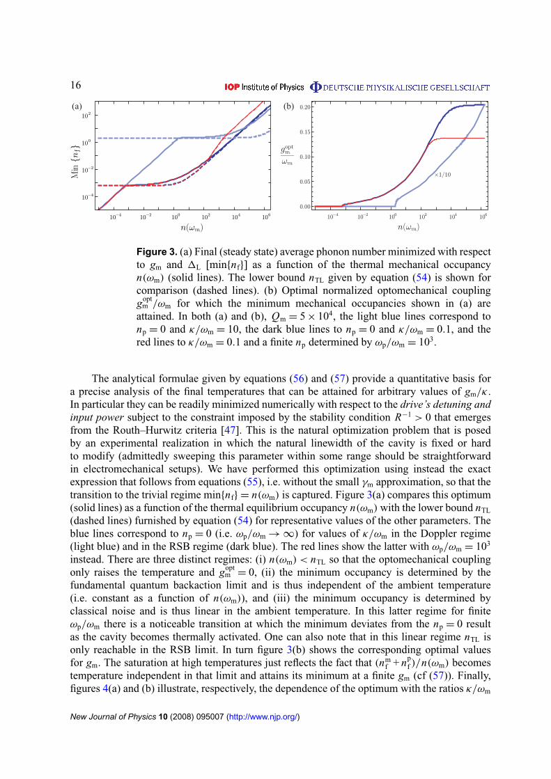
Figure 3. (a) Final (steady state) average phonon number minimized with respectto gm and 1L [min{nf}] as a function of the thermal mechanical occupancyn(ωm) (solid lines). The lower bound nTL given by equation (54) is shown forcomparison (dashed lines). (b) Optimal normalized optomechanical couplinggopt
m /ωm for which the minimum mechanical occupancies shown in (a) areattained. In both (a) and (b), Qm = 5 × 10⁴, the light blue lines correspond tonp = 0 and κ/ωm = 10, the dark blue lines to np = 0 and κ/ωm = 0.1, and thered lines to κ/ωm = 0.1 and a finite np determined by ωp/ωm = 103.
The analytical formulae given by equations (56) and (57) provide a quantitative basis fora precise analysis of the final temperatures that can be attained for arbitrary values of gm/κ .In particular they can be readily minimized numerically with respect to the drive’s detuning andinput power subject to the constraint imposed by the stability condition R−1 > 0 that emergesfrom the Routh–Hurwitz criteria [47]. This is the natural optimization problem that is posedby an experimental realization in which the natural linewidth of the cavity is fixed or hardto modify (admittedly sweeping this parameter within some range should be straightforwardin electromechanical setups). We have performed this optimization using instead the exactexpression that follows from equations (55), i.e. without the small γm approximation, so that thetransition to the trivial regime min{nf} = n(ωm) is captured. Figure 3(a) compares this optimum(solid lines) as a function of the thermal equilibrium occupancy n(ωm) with the lower bound nTL
(dashed lines) furnished by equation (54) for representative values of the other parameters. Theblue lines correspond to np = 0 (i.e. ωp/ωm → ∞) for values of κ/ωm in the Doppler regime(light blue) and in the RSB regime (dark blue). The red lines show the latter with ωp/ωm = 103
instead. There are three distinct regimes: (i) n(ωm) < nTL so that the optomechanical couplingonly raises the temperature and gopt
m = 0, (ii) the minimum occupancy is determined by thefundamental quantum backaction limit and is thus independent of the ambient temperature(i.e. constant as a function of n(ωm)), and (iii) the minimum occupancy is determined byclassical noise and is thus linear in the ambient temperature. In this latter regime for finiteωp/ωm there is a noticeable transition at which the minimum deviates from the np = 0 resultas the cavity becomes thermally activated. One can also note that in this linear regime nTL isonly reachable in the RSB limit. In turn figure 3(b) shows the corresponding optimal valuesfor gm. The saturation at high temperatures just reflects the fact that (nm
f + npf )/n(ωm) becomes
temperature independent in that limit and attains its minimum at a finite gm (cf (57)). Finally,figures 4(a) and (b) illustrate, respectively, the dependence of the optimum with the ratios κ/ωm
New Journal of Physics 10 (2008) 095007 (http://www.njp.org/)
17
ωpωm
κ
ωm
n(ωm)10−4 10−2 100 102 104 106
101
102
103
104
105
106
107
100101
102
103
104
10−1
10−2
10−3
n(ωm)
−
−
−
−
−
−−
10−3
10−2
10−1 100
101
102
1
1
2
4
6
8
0
0
1
1
1
1
1
22 44 6
10
10
10
10
10
10
101010101010
×
×
×
×
×
×
(a) (b)
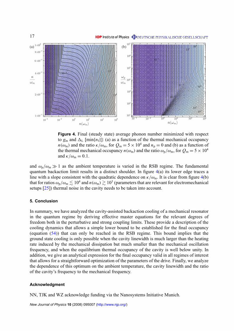
Figure 4. Final (steady state) average phonon number minimized with respectto gm and 1L [min{nf}]: (a) as a function of the thermal mechanical occupancyn(ωm) and the ratio κ/ωm, for Qm = 5 × 10⁴ and np = 0 and (b) as a function ofthe thermal mechanical occupancy n(ωm) and the ratio ωp/ωm, for Qm = 5 × 10⁴
and κ/ωm = 0.1.
and ωp/ωm � 1 as the ambient temperature is varied in the RSB regime. The fundamentalquantum backaction limit results in a distinct shoulder. In figure 4(a) its lower edge traces aline with a slope consistent with the quadratic dependence on κ/ωm. It is clear from figure 4(b)that for ratios ωp/ωm . 104 and n(ωm)& 103 (parameters that are relevant for electromechanicalsetups [25]) thermal noise in the cavity needs to be taken into account.
5. Conclusion
In summary, we have analyzed the cavity-assisted backaction cooling of a mechanical resonatorin the quantum regime by deriving effective master equations for the relevant degrees offreedom both in the perturbative and strong coupling limits. These provide a description of thecooling dynamics that allows a simple lower bound to be established for the final occupancy(equation (54)) that can only be reached in the RSB regime. This bound implies that theground state cooling is only possible when the cavity linewidth is much larger than the heatingrate induced by the mechanical dissipation but much smaller than the mechanical oscillationfrequency, and when the equilibrium thermal occupancy of the cavity is well below unity. Inaddition, we give an analytical expression for the final occupancy valid in all regimes of interestthat allows for a straightforward optimization of the parameters of the drive. Finally, we analyzethe dependence of this optimum on the ambient temperature, the cavity linewidth and the ratioof the cavity’s frequency to the mechanical frequency.
Acknowledgment
NN, TJK and WZ acknowledge funding via the Nanosystems Initiative Munich.
New Journal of Physics 10 (2008) 095007 (http://www.njp.org/)
18
References
[1] Craighead H G 2000 Nanoelectromechanical systems Science 290 1532[2] Ekinci K L and Roukes M L 2005 Nanoelectromechanical systems Rev. Sci. Instrum. 76 061101[3] Braginsky V B 1977 Measurement of Weak Forces in Physics Experiments (Chicago: University of
Chicago Press)[4] Kippenberg T J and Vahala K J 2007 Cavity opto-mechanics Opt. Express 15 17172[5] LaHaye M D, Buu O, Camarota B and Schwab K C 2004 Approaching the quantum limit of a nanomechanical
resonator Science 304 74[6] Knobel R G and Cleland A N 2003 Nanometer-scale displacement sensing using a single electron transistor
Nature 424 291[7] Caves C M 1981 Quantum-mechanical noise in an interferometer Phys. Rev. D 23 1693[8] Abramovici A et al 1992 Ligo—the laser-interferometer-gravitational-wave-observatory Science 256 325[9] Milburn G J, Jacobs K and Walls D F 1994 Quantum-limited measurements with the atomic force microscope
Phys. Rev. A 50 5256[10] Bocko M F and Onofrio R 1996 On the measurement of a weak classical force coupled to a harmonic
oscillator: experimental progress Rev. Mod. Phys. 68 755[11] Blencowe M P and Buks E 2007 Quantum analysis of a linear dc SQUID mechanical displacement detector
Phys. Rev. B 76 014511[12] Sidles J A, Garbini J L, Bruland K J, Rugar D, Züger O, Hoen S and Yannoni C S 1995 Magnetic resonance
force microscopy Rev. Mod. Phys. 67 249[13] Gassmann H, Choi M-S, Yi H and Bruder C 2004 Quantum dissipative dynamics of the magnetic resonance
force microscope in the single-spin detection limit Phys. Rev. B 69 115419[14] Schwab K C and Roukes M L 2005 Putting mechanics into quantum mechanics Phys. Today 58 36[15] Vitali D, Gigan S, Ferreira A, Bohm H R, Tombesi P, Guerreiro A, Vedral V, Zeilinger A and Aspelmeyer
M 2007 Optomechanical entanglement between a movable mirror and a cavity field Phys. Rev. Lett.98 030405
[16] Vitali D, Tombesi P, Woolley M J, Doherty A C and Milburn G J 2007 Entangling a nanomechanical resonatorand a superconducting microwave cavity Phys. Rev. A 76 042336
[17] Mancini S, Vitali D and Tombesi P 1998 Optomechanical cooling of a macroscopic oscillator by homodynefeedback Phys. Rev. Lett. 80 688
[18] Cohadon P F, Heidmann A and Pinard M 1999 Cooling of a mirror by radiation pressure Phys. Rev. Lett.83 3174
[19] Hoehberger-Metzger C H and Karrai K 2004 Cavity cooling of a microlever Nature 432 1002[20] Naik A, Buu O, LaHaye M D, Armour A D, Clerk A A, Blencowe M P and Schwab K C 2006 Cooling a
nanomechanical resonator with quantum back-action Nature 443 193[21] Gigan S, Böhm H R, Paternostro M, Blaser F, Langer G, Hertzberg J B, Schwab K C, Bäuerle D, Aspelmeyer
M and Zeilinger A 2006 Self-cooling of a micromirror by radiation pressure Nature 444 67[22] Arcizet O, Cohadon P-F, Briant T, Pinard M and Heidmann A 2006 Radiation-pressure cooling and
optomechanical instability of a micromirror Nature 444 71[23] Kleckner D and Bouwmeester D 2006 Sub-kelvin optical cooling of a micromechanical resonator Nature
444 75[24] Schliesser A, DelHaye P, Nooshi N, Vahala K J and Kippenberg T J 2006 Radiation pressure cooling of a
micromechanical oscillator using dynamical backaction Phys. Rev. Lett. 97 243905[25] Brown K R, Britton J, Epstein R J, Chiaverini J, Leibfried D and Wineland D J 2007 Passive cooling of a
micromechanical oscillator with a resonant electric circuit Phys. Rev. Lett. 99 137205[26] Poggio M, Degen C L, Mamin H J and Rugar D 2007 Feedback cooling of a cantilever’s fundamental mode
below 5 mK Phys. Rev. Lett. 99 017201[27] Thompson J D, Zwickl B M, Jayich A M, Marquardt F, Girvin S M and Harris J G E 2008 Strong dispersive
coupling of a high finesse cavity to a micromechanical membrane Nature 452 72
New Journal of Physics 10 (2008) 095007 (http://www.njp.org/)
19
[28] Schliesser A, Rivière R, Anetsberger G, Arcizet O and Kippenberg T J 2008 Resolved sideband cooling of amicromechanical oscillator Nat. Phys. 4 415
[29] Teufel J D, Regal C A and Lehnert K W 2008 Prospects for cooling nanomechanical motion by coupling to asuperconducting microwave resonator New J. Phys. 10 095002
[30] Wineland D J and Itano W M 1979 Laser cooling of atoms Phys. Rev. A 20 1521[31] Stenholm S 1986 The semiclassical theory of laser cooling Rev. Mod. Phys. 58 699[32] Leibfried D, Blatt R, Monroe C and Wineland D 2003 Quantum dynamics of single trapped ions Rev. Mod.
Phys. 75 281[33] Ashkin A 1997 Optical trapping and manipulation of neutral particles using lasers Proc. Natl Acad. Sci. USA
94 4853–60[34] Braginsky V B and Vyatchanin S P 2002 Low quantum noise tranquilizer for Fabry–Perot interferometer
Phys. Lett. A 293 228[35] Caves C M, Thorne K S, Drever R W P, Sandberg V D and Zimmermann M 1980 On the measurement of
a weak classical force coupled to a quantum-mechanical oscillator. 1. Issues of principle Rev. Mod. Phys.52 341–92
[36] Braginsky V B and Khalili F Y 1992 Quantum Measurement (Cambridge: Cambridge University Press)[37] Braginsky V B and Khalili F Y 1996 Quantum nondemolition measurements: the route from toys to tools
Rev. Mod. Phys. 68 1–10[38] Martin I, Shnirman A, Tian L and Zoller P 2004 Ground-state cooling of mechanical resonators Phys. Rev. B
69 125339[39] Wilson-Rae I, Zoller P and Imamoglu A 2004 Laser cooling of a nanomechanical resonator mode to its
quantum ground state Phys. Rev. Lett. 92 075507[40] Kippenberg T J, Rokhsari H, Carmon T, Scherer A and Vahala K J 2005 Analysis of radiation-pressure
induced mechanical oscillation of an optical microcavity Phys. Rev. Lett. 95 033901[41] Wilson-Rae I, Nooshi N, Zwerger W and Kippenberg T J 2007 Theory of ground state cooling of a mechanical
oscillator using dynamical backaction Phys. Rev. Lett. 99 093901[42] Marquardt F, Chen J P, Clerk A A and Girvin S M 2007 Quantum theory of cavity-assisted sideband cooling
of mechanical motion Phys. Rev. Lett. 99 093902[43] Bhattacharya M and Meystre P 2007 Trapping and cooling a mirror to its quantum mechanical ground state
Phys. Rev. Lett. 99 073601[44] Marquardt F, Harris J G E and Girvin S M 2006 Dynamical multistability induced by radiation pressure in
high-finesse micromechanical optical cavities Phys. Rev. Lett. 96 103901[45] Law C K 1995 Interaction between a moving mirror and radiation pressure—a Hamiltonian—formulation
Phys. Rev. A 51 2537[46] Gardiner C W and Zoller P 2004 Quantum Noise (Berlin: Springer)[47] DeJesus E X and Kaufmann C 1987 Routh–Hurwitz criterion in the examination of eigenvalues of a system
of nonlinear ordinary differential equations Phys. Rev. A 35 5288[48] Cleland A N 2003 Foundations of Nanomechanics (Berlin: Springer)[49] Wilson-Rae I 2008 Intrinsic dissipation in nanomechanical resonators due to phonon tunneling Phys. Rev. B
77 245418[50] Zwanzig R 1964 On the identity of three generalized master equations Physica 30 1109[51] Cirac J I, Blatt R, Zoller P and Phillips W D 1992 Laser cooling of trapped ions in a standing wave Phys.
Rev. A 46 2668
New Journal of Physics 10 (2008) 095007 (http://www.njp.org/)