Embed Size (px)
Citation preview
New Insights in Prediction and Dynamic Modeling from Non-Gaussian Mixture Processing Methods
DOCTORAL THESIS
by
Gonzalo Safont Armero
Supervisors:
Dr. Addisson Salazar Afanador
Dr. Luis Vergara Domínguez
Valencia, Spain
July 2015

New Insights in Prediction and Dynamic Modeling from Non-Gaussian Mixture Processing Methods
by
Gonzalo Safont Armero
THESIS
Submitted in fulfillment of the requirements for the degree of Doctor of
Philosophy in Telecommunications in the Departamento de
Comunicaciones of the Universitat Politècnica de València
Supervisors:
Dr. Addisson Salazar Afanador
Dr. Luis Vergara Domínguez
Departamento de
Comunicaciones Instituto de Telecomunicaciones
y Aplicaciones Multimedia Grupo de Tratamiento
de Señal
UNIVERSITAT POLITÈCNICA DE VALÈNCIA
DEPARTAMENTO DE COMUNICACIONES
Valencia, Spain
July 2015


To Marta


“Intelligence is nothing more than discussing things with others.
Limitless wisdom comes of this.”
—Yamamoto Tsunetomo, Hagakure (In the Shadow of Leaves)


i
Abstract
This thesis considers new applications of non-Gaussian mixtures in the framework of statistical
signal processing and pattern recognition. The non-Gaussian mixtures were implemented by
mixtures of independent component analyzers (ICA). The fundamental hypothesis of ICA is that
the observed signals can be expressed as a linear transformation of a set of hidden variables,
usually referred to as sources, which are statistically independent. This independence allows
factoring the original M-dimensional probability density function (PDF) of the data as a product
of one-dimensional probability densities, greatly simplifying the modeling of the data. ICA
mixture models (ICAMM) provide further flexibility by alleviating the independency
requirement of ICA, thus allowing the model to obtain local projections of the data without
compromising its generalization capabilities. Here are explored new possibilities of ICAMM for
the purposes of estimation and classification of signals.
The thesis makes several contributions to the research in non-Gaussian mixtures: (i) a method
for maximum-likelihood estimation of missing data, based on the maximization of the PDF of
the data given the ICAMM; (ii) a method for Bayesian estimation of missing data that
minimizes the mean squared error and can obtain the confidence interval of the prediction; (iii)
a generalization of the sequential dependence model for ICAMM to semi-supervised or
supervised learning and multiple chains of dependence, thus allowing the use of multimodal
data; and (iv) introduction of ICAMM in diverse novel applications, both for estimation and for
classification.
The developed methods were validated via an extensive number of simulations that covered
multiple scenarios. These tested the sensitivity of the proposed methods with respect to the
following parameters: number of values to estimate; kinds of source distributions;
correspondence of the data with respect to the assumptions of the model; number of classes in
the mixture model; and unsupervised, semi-supervised, and supervised learning. The
performance of the proposed methods was evaluated using several figures of merit, and
compared with the performance of multiple classical and state-of-the-art techniques for
estimation and classification.
Aside from the simulations, the methods were also tested on several sets of real data from
different types: data from seismic exploration studies; ground penetrating radar surveys; and
biomedical data. These data correspond to the following applications: reconstruction of
damaged or missing data from ground-penetrating radar surveys of historical walls;
reconstruction of damaged or missing data from a seismic exploration survey; reconstruction of
artifacted or missing electroencephalographic (EEG) data; diagnosis of sleep disorders;
modeling of the brain response during memory tasks; and exploration of EEG data from
subjects performing a battery of neuropsychological tests. The obtained results demonstrate the
capability of the proposed methods to work on problems with real data. Furthermore, the
proposed methods are general-purpose and can be used in many signal processing fields.


iii
Resum
Aquesta tesi considera noves aplicacions de barreges no Gaussianes dins del marc de treball del
processament estadístic de senyal i del reconeixement de patrons. Les barreges no Gaussianes
van ser implementades mitjançant barreges d’analitzadors de components independents (ICA).
La hipòtesi fonamental d’ICA és que els senyals observats poden ser expressats com una
transformació lineal d’un grup de variables ocultes, comunament anomenades fonts, que són
estadísticament independents. Aquesta independència permet factoritzar la funció de densitat de
probabilitat (PDF) original M–dimensional de les dades com un producte de densitats de
probabilitat unidimensionals, simplificant àmpliament la modelització de les dades. Els models
de barreges ICA (ICAMM) aporten una major flexibilitat en alleugerar el requeriment
d’independència d’ICA, permetent així que el model obtinga projeccions locals de les dades
sense comprometre la seva capacitat de generalització. Ací s’exploren noves possibilitats
d’ICAMM pels propòsits d’estimació i classificació de senyals.
Aquesta tesi aporta diverses contribucions a la recerca en barreges no Gaussianes: (i) un mètode
d’estimació de dades faltants per màxima versemblança, basat en la maximització de la PDF de
les dades donat l’ICAMM; (ii) un mètode d’estimació Bayesiana de dades faltants que
minimitza l’error quadràtic mitjà i pot obtenir l’interval de confiança de la predicció; (iii) una
generalització del model de dependència seqüencial d’ICAMM per entrenament supervisat o
semi-supervisat i múltiples cadenes de dependència, permetent així l’ús de dades multimodals; i
(iv) introducció d’ICAMM en diverses noves aplicacions, tant per a estimació com per a
classificació.
Els mètodes desenvolupats van ser validats mitjançant una extensa quantitat de simulacions que
cobriren múltiples situacions. Aquestes van verificar la sensibilitat dels mètodes proposats amb
respecte als següents paràmetres: nombre de valors per estimar; mena de distribucions de les
fonts; correspondència de les dades amb respecte a les suposicions del model; nombre de
classes del model de barreges; i aprenentatge supervisat, semi-supervisat i no-supervisat. El
rendiment dels mètodes proposats va ser avaluat mitjançant diverses figures de mèrit, i comparat
amb el rendiments de múltiples tècniques clàssiques i de l’estat de l’art per a estimació i
classificació.
A banda de les simulacions, els mètodes van ser verificats també sobre diversos grups de dades
reals de diferents tipus: dades d’estudis d’exploració sísmica; exploracions de radars de
penetració de terra; i dades biomèdiques. Aquestes dades corresponen a les següents
aplicacions: reconstrucció de dades danyades o faltants d’estudis d’exploracions de radar de
penetració de terra sobre murs històrics; reconstrucció de dades danyades o faltants en un estudi
d’exploració sísmica; reconstrucció de dades electroencefalogràfiques (EEG) artefactuades o
faltants; diagnosi de desordres de la son; modelització de la resposta del cervell durant tasques
de memòria; i exploració de dades EEG de subjectes realitzant una bateria de tests
neuropsicològics. Els resultats obtinguts han demostrat la capacitat dels mètodes proposats per
treballar en problemes amb dades reals. A més, els mètodes proposats són de propòsit general i
poden fer-se servir en molts camps del processament de senyal.


v
Resumen
Esta tesis considera nuevas aplicaciones de las mezclas no Gaussianas dentro del marco de
trabajo del procesado estadístico de señal y del reconocimiento de patrones. Las mezclas no
Gaussianas fueron implementadas mediante mezclas de analizadores de componentes
independientes (ICA). La hipótesis fundamental de ICA es que las señales observadas pueden
expresarse como una transformación lineal de un grupo de variables ocultas, normalmente
llamadas fuentes, que son estadísticamente independientes. Esta independencia permite
factorizar la función de densidad de probabilidad (PDF) original M–dimensional de los datos
como un producto de densidades unidimensionales, simplificando ampliamente el modelado de
los datos. Los modelos de mezclas ICA (ICAMM) aportan una mayor flexibilidad al relajar el
requisito de independencia de ICA, permitiendo que el modelo obtenga proyecciones locales de
los datos sin comprometer su capacidad de generalización. Aquí se exploran nuevas
posibilidades de ICAMM para los propósitos de estimación y clasificación de señales.
La tesis realiza varias contribuciones a la investigación en mezclas no Gaussianas: (i) un método
de estimación de datos faltantes por máxima verosimilitud, basado en la maximización de la
PDF de los datos dado el ICAMM; (ii) un método de estimación Bayesiana de datos faltantes
que minimiza el error cuadrático medio y puede obtener el intervalo de confianza de la
predicción; (iii) una generalización del modelo de dependencia secuencial de ICAMM para
aprendizaje supervisado o semi-supervisado y múltiples cadenas de dependencia, permitiendo
así el uso de datos multimodales; y (iv) introducción de ICAMM en varias aplicaciones
novedosas, tanto para estimación como para clasificación.
Los métodos desarrollados fueron validados mediante un número extenso de simulaciones que
cubrieron múltiples escenarios. Éstos comprobaron la sensibilidad de los métodos propuestos
con respecto a los siguientes parámetros: número de valores a estimar; tipo de distribuciones de
las fuentes; correspondencia de los datos con respecto a las suposiciones del modelo; número de
clases en el modelo de mezclas; y aprendizaje supervisado, semi-supervisado y no supervisado.
El rendimiento de los métodos propuestos fue evaluado usando varias figuras de mérito, y
comparado con el rendimiento de múltiples técnicas clásicas y del estado del arte para
estimación y clasificación.
Además de las simulaciones, los métodos también fueron probados sobre varios grupos de datos
de diferente tipo: datos de estudios de exploración sísmica; exploraciones por radar de
penetración terrestre; y datos biomédicos. Estos datos corresponden a las siguientes
aplicaciones: reconstrucción de datos dañados o faltantes de exploraciones de radar de
penetración terrestre de muros históricos; reconstrucción de datos dañados o faltantes de un
estudio de exploración sísmica; reconstrucción de datos electroencefalográficos (EEG) dañados
o artefactados; diagnóstico de desórdenes del sueño; modelado de la respuesta del cerebro
durante tareas de memoria; y exploración de datos EEG de sujetos durante la realización de una
batería de pruebas neuropsicológicas. Los resultados obtenidos demuestran la capacidad de los
métodos propuestos para trabajar en problemas con datos reales. Además, los métodos
propuestos son de propósito general y pueden utilizarse en muchos campos del procesado de
señal.


vii
Acknowledgment
First and foremost, I would like to thank my advisors, Addisson Salazar and Luis Vergara, for
their support and guidance throughout the making of this thesis. Their expertise and research
have been truly invaluable for this work and for my growth as a researcher. The years we have
spent on this thesis have introduced me to research and the world of academia. Furthermore, it
has also allowed me to work with many different types of signals and learn many different
techniques and methods, an opportunity I would not have had without their faith in me. Our
discussions have deeply enriched my knowledge of research and signal processing, and some
more eclectic topics (from soccer to philosophy and literature).
I would like to express my gratitude to Christian Jutten, who allowed me to stay at his lab at the
Université Joseph Fourier, for his valuable comments and insights about this work. These
thanks include Ladan Amini and the rest of the GIPSA-lab, whose efforts and help made me
feel at home during my stay at Grenoble.
I would also like to thank my coworkers throughout these years at Grupo de Tratamiento de
Señal (GTS), in no particular order: Arturo, Jorge, Martín, Raquel, María Ángeles, Vicky,
Vicente, Màriam, Beni, Patricia, Juan, Alicia, Guillermo, Ahmed, and all the people at GTS.
David and Elena too; although you guys are not part of the GTS, you might as well be for all the
time we have been together! I would like to offer a (posthumous) thanks to the
Terrasseta/Malvarosa restaurant where we used to have breakfast every Thursday (except when
it was not a Thursday). Restaurant, you are sorely missed.
I would also like to thank my friends during these years: Paco, Francesc, Toni, and Ana from
Telecommunications Engineering, but also Martí, Borja, Carlos, Antonio, and Eva from Civil
Engineering.
Thanks to my family (both my own and my in-laws) for their love and support.
I would also like to acknowledge the support of the Spanish Government and Universitat
Politècnica de València for the grants that I have enjoyed, which have made this thesis possible.
Finally, a very special thank you for Marta. Words cannot describe how grateful I am that I met
you. Now you have to thank me back in your thesis!

ix
Table of contents
- Introduction ................................................................................................................ 3
1.1. Review of methods ............................................................................................................. 6
1.1.1. Estimation ................................................................................................................... 6 1.1.2. Probability density estimation ..................................................................................... 9 1.1.3. Statistical classification ............................................................................................. 11 1.1.4. Non-linear dynamic modeling ................................................................................... 14
1.2. Scope ................................................................................................................................ 15
1.3. Contributions .................................................................................................................... 16
1.3.1. Interpolation based on ICA and ICA mixture models ............................................... 16 1.3.2. Sequential dynamic modeling ................................................................................... 17 1.3.3. New applications of ICA and ICAMM ..................................................................... 17
1.4. Overview .......................................................................................................................... 19
- Finite mixture models with non-Gaussian components ........................................... 23
2.1. Introduction ...................................................................................................................... 23
2.2. Univariate non-Gaussian mixtures ................................................................................... 26
2.2.1. Mixtures of Exponential Distributions ...................................................................... 26 2.2.2. Mixtures of Poisson distributions .............................................................................. 27 2.2.3. Mixtures of binomial distributions ............................................................................ 28 2.2.4. Mixtures of multinomial distributions ....................................................................... 29
2.3. Multivariate non-Gaussian ............................................................................................... 29
2.3.1. Copula functions ....................................................................................................... 29 2.3.2. Latent variable modeling ........................................................................................... 32 2.3.3. Independent component analysis (ICA) .................................................................... 37
2.4. Mixtures of independent component analyzers ................................................................ 39
2.4.1. Definition .................................................................................................................. 39 2.4.2. Maximum likelihood ................................................................................................. 42 2.4.3. Beta-divergence ......................................................................................................... 42 2.4.4. Variational Bayesian ................................................................................................. 43 2.4.5. Non-Parametric ......................................................................................................... 43
2.5. Conclusions ...................................................................................................................... 44
- Building non-linear prediction structures from independent component analysis ... 49
3.1. Prediction based on maximum likelihood: PREDICAMM .............................................. 51
3.1.1. Optimization procedure ............................................................................................. 53
3.2. Prediction based on least mean squared error: E-ICAMM .............................................. 54
3.2.1. Bias and local prediction error of E-ICAMM ........................................................... 57
3.3. Other methods .................................................................................................................. 60
3.3.1. Kriging ...................................................................................................................... 60 3.3.2. Wiener structures....................................................................................................... 62 3.3.3. Matrix completion based on smoothed rank function (SRF) .................................... 64 3.3.4. Splines ....................................................................................................................... 65
3.4. Simulations ....................................................................................................................... 67

x
3.4.1. Problem description................................................................................................... 67 3.4.2. Error indicators .......................................................................................................... 69 3.4.3. Parameter setting for PREDICAMM ........................................................................ 71 3.4.4. Simulation on data from ICA mixture models .......................................................... 76 3.4.5. Simulation on data from ICA mixture models with random nonlinearities .............. 79 3.4.6. Simulation with an increasing number of missing traces .......................................... 82
3.5. Conclusions ...................................................................................................................... 85
- A general dynamic modeling approach based on synchronized ICA mixture models:
G- and UG-SICAMM ................................................................................................................. 89
4.1. Sequential ICA mixture model: SICAMM ...................................................................... 90
4.1.1. Training algorithm..................................................................................................... 93 4.1.2. SICAMM variants ..................................................................................................... 93
4.2. Generalized SICAMM: G-SICAMM ............................................................................... 97
4.2.1. The model and the definition of the problem ............................................................ 97 4.2.2. Training algorithm................................................................................................... 100 4.2.3. G-SICAMM variants ............................................................................................... 100
4.3. Unsupervised Generalized SICAMM: UG-SICAMM ................................................... 101
4.3.1. The log-likelihood cost function ............................................................................. 101 4.3.2. UG-SICAMM algorithm ......................................................................................... 105 4.3.3. Non-parametric estimation of the source densities ................................................. 107 4.3.4. Semi-supervised training ......................................................................................... 108
4.4. State of the art methods .................................................................................................. 109
4.4.1. Bayesian Networks .................................................................................................. 109 4.4.2. Dynamic Bayesian Networks .................................................................................. 110
4.5. Simulations ..................................................................................................................... 111
4.5.1. Measuring the distance between two G-SICAMMs ................................................ 111 4.5.2. Simulation of UG-SICAMM for semi-supervised training ..................................... 113 4.5.3. Simulation of SICAMM and G-SICAMM variants ................................................ 115
4.6. Conclusions .................................................................................................................... 122
- Application of PREDICAMM to non-destructive testing and EEG signal processing
applications ............................................................................................................................... 127
5.1. Non-destructive testing simulations ............................................................................... 128
5.1.1. Ground-penetrating radar ........................................................................................ 129 5.1.2. Preprocessing of the B-Scan for ICAMM: data alignment ..................................... 131 5.1.3. Simulations .............................................................................................................. 132
5.2. Application on GPR data from a survey on historical walls .......................................... 137
5.3. Application on seismic signals for underground surveying ........................................... 141
5.3.1. Reconstruction of seismic data ................................................................................ 142
5.4. Application on electroencephalographic signals ............................................................ 145
5.4.1. Data capture ............................................................................................................ 146 5.4.2. Sternberg memory task............................................................................................ 147 5.4.3. Reconstruction of missing EEG data....................................................................... 148
5.5. Conclusions .................................................................................................................... 151
xi
- Application of G- and UG-SICAMM to EEG signal processing ........................... 155
6.1. Automatic classification of hypnogram data .................................................................. 156
6.1.1. Data and pre-processing .......................................................................................... 157 6.1.2. Classification results ............................................................................................... 159 6.1.3. Sensitivity analysis .................................................................................................. 160
6.2. Analysis of EEG data captured during a working memory task .................................... 160
6.2.1. Experiment configuration ........................................................................................ 163 6.2.2. Classification results ............................................................................................... 169 6.2.3. Sensitivity analysis .................................................................................................. 172
6.3. Analysis of EEG data from neurophysiological tests ..................................................... 173
6.3.1. Neuropsychological tests......................................................................................... 175 6.3.2. Experiment configuration ........................................................................................ 179 6.3.3. Classification results ............................................................................................... 182 6.3.4. Exploratory results .................................................................................................. 187
6.4. Conclusions .................................................................................................................... 189
- Conclusions and future work .................................................................................. 193
7.1. Summary ........................................................................................................................ 193
7.2. Contributions to knowledge ........................................................................................... 195
7.3. Future work .................................................................................................................... 196
Data estimation methods ................................................................................................... 196 Dynamic modeling methods.............................................................................................. 197 Other applications ............................................................................................................. 197
7.4. List of publications ......................................................................................................... 197
Refereed JCR journals ....................................................................................................... 197 Book chapters .................................................................................................................... 198 Peer-reviewed non-JCR journals ....................................................................................... 198 International conferences .................................................................................................. 198 National (Spanish) conferences ......................................................................................... 199
Appendix 1 – Classification results for the neuropsychological experiment ............................ 203
Two-class classification ........................................................................................................ 203
Three-class classification ...................................................................................................... 208
References ................................................................................................................................. 215
xii
List of tables and figures
Figure 1.1. Diagram explaining the estimation problem. ...................................................................... 6
Figure 1.2. Comparison of the joint density of one-dimensional observations, x, with respect to a
parameter α. The concentrical ovals denote points of equal density, with higher PDF being more
yellow. The plots on the side of the joint density show the PDF of α and the likelihood of x for the
most common value of α. Note that the maximum of the joint density (denoted by the two dashed
lines) yields a different solution than the maximum of the likelihood function (denoted by the red
square), particularly for x. ..................................................................................................................... 8
Table 1.1. Typical kernel functions used for kernel density estimation. ............................................ 10
Figure 1.3. Illustrative example of the effect of bandwidth selection on kernel density estimation. .. 11
Figure 1.4. Statistical classification process. ...................................................................................... 12
Figure 1.5. Approaches to statistical classification. Shadowed boxes indicate the approaches
considered in this work. ...................................................................................................................... 13
Figure 1.6. A basic dynamic model that relates hidden states, yt, with observation vectors, xt. ......... 14
Figure 2.1. Scheme of multivariate finite mixture models. ................................................................. 25
Figure 2.2. Examples of univariate non-Gausian mixtures. ................................................................ 26
Figure 2.3. Example of PDF modeling of two random variables using copulas. ................................ 31
Table 2.1. Types of latent variable models. ........................................................................................ 33
Figure 2.4. Example of probabilistic graphical models for a mixture of two Gaussians (dashed-line
nodes are observed variables, continuous-line nodes are latent (hidden) variables, and double-line
nodes are fixed hyper-parameters). ..................................................................................................... 34
Figure 2.5. Example of an independent cluster factor model.............................................................. 36
Figure 2.6. Independent component analysis model with two sources and two recorded variables (M
= 2). The color of the arrows denotes the weight of the corresponding component/source: dark colors
are higher than light colors. ................................................................................................................ 38
Figure 2.7. Outline of the ICA mixture model as a switching model of K separate ICA models. ...... 40
Figure 2.8. Comparison of ICA versus ICAMM for a source separation task: a) two sources are
mixed with two classes to obtain two recorded variables, which are then separated by a two-class
ICAMM; b) result of ICA for the same source separation task. The colors of the mixing/de-mixing
matrices denote the weight of the corresponding element: dark colors are higher than light colors. . 40
Figure 2.9. Estimation of an ICA mixture model with two classes (frog and text). Each class
produces a different ICA, as shown by their different mixing matrices and centroids. ...................... 41
Figure 2.10. Segmentation of an image using ICAMM. ..................................................................... 41
Table 2.2. Non-parametric learning algorithm. ................................................................................... 44
Figure 3.1. Sampling schemes for use in PREDICAMM and E-ICAMM: a) time; b) space; c)
windows or patches; d) diagonal. The empty green rectangles represent all the data, areas shadowed
in green denote the current observation, areas enclosed in dotted lines represent other observations,
and black areas denote missing values. Dotted arrows show some possible sweeping trajectories to
reconstruct all missing data. ................................................................................................................ 50
Figure 3.2. General definition of the prediction process using PREDICAMM and E-ICAMM. Note
that there are several method configurations that we can use, which will be explained in Section
3.4.3.b. The asterisks denote the original contributions in this work. ................................................. 51
Table 3.1. Iterative algorithm to compute the conditional expectation E[z|y, Ck]. ............................. 55
Figure 3.3. E-ICAMM reconstruction for two toy examples: a) data drawn from an ICAMM with
two classes; b) horseshoe-shaped unlabeled data modeled using an ICAMM with five classes. ....... 56
Table 3.2. Iterative algorithm to compute the conditional covariance E[z·zT|y, Ck]. .......................... 59
Figure 3.4. Estimated local prediction error for E-ICAMM for the two toy examples in Figure 3.3. 59

xiii
Figure 3.5. Wiener structure (top), Hammerstein structure (middle), and Wiener-Hammerstein
structure (bottom). .............................................................................................................................. 63
Figure 3.6. Different method configurations considered during the simulations in this chapter. The
shaded boxes represent the original contributions of this thesis. ........................................................ 67
Table 3.3. Data distributions used for simulation. .............................................................................. 68
Table 3.4. Details of all datasets used in the simulated experiment. ................................................... 68
Figure 3.7. Graphical description of the prediction problem. The hatched area indicates missing data.
............................................................................................................................................................ 69
Table 3.5. Summary of the prediction error indicators considered in this work. ................................ 70
Figure 3.8. Diagram showing each iteration of the Monte Carlo experiment for the simulation. This
process is repeated a number of times during each Monte Carlo experiment. .................................... 72
Figure 3.9. Stability of the prediction in a case with one unknown variable and one class. a) output
variable, normalized with respect to the true result; b) number of iterations taken. For reference, a
perfect solution would mean that the output variable is always equal to 0, and the number of
iterations would always be close to 0.................................................................................................. 73
Figure 3.10. Stability of the prediction for the case with one unknown variable and two classes. a)
output variable, normalized with respect to the true result; b) number of iterations taken. For
reference, a perfect solution would mean that the output variable is always equal to 0, and the
number of iterations would always be close to 0. ............................................................................... 73
Figure 3.11. Stability of the prediction for the case with two unknown variables and two classes. a)
number of iterations taken; b) normalized value of the first output variable after convergence; c)
normalized value of the second output variable after convergence. For reference, a perfect solution
would mean that the output variable is always equal to 0 and the number of iterations would always
be close to 0; in the above, it would correspond to dark blue areas in all three sub-Figures. ............. 74
Figure 3.12. Joint probability densities with respect to the number of iterations, depending on the
number of classes in the model (single, two or three classes)............................................................. 74
Table 3.6. Comparative study between the three considered variants of the steepest ascent method. 74
Figure 3.13. Error indicators for the proposed initial values for PREDICAMM. ............................... 75
Figure 3.14. Typical prediction result for dataset #3: a) true data; b) predictions obtained by the
methods with worst performance; c) predictions obtained by the methods with best performance. .. 76
Figure 3.15. Error indicators for the single-class datasets. ................................................................. 77
Figure 3.16. Typical prediction result for one of the variables of dataset #13. ................................... 78
Figure 3.17. Error indicators for the multiple-class datasets............................................................... 78
Figure 3.18. Diagram showing the process of each iteration of the Monte Carlo experiment with
nonlinear data. This process is repeated several times during each Monte Carlo experiment. Note that
the third step, where data are corrupted with a nonlinearity, is what separates it from the Monte
Carlo experiment in Section 3.4.4. ...................................................................................................... 79
Figure 3.19. Error indicators for the proposed methods with respect to the distortion rate of a single-
class ICA (mixture) model, dataset #4. ............................................................................................... 80
Figure 3.20. Error indicators for the proposed methods with respect to the distortion rate of a two-
class ICAMM, dataset #9. ................................................................................................................... 81
Figure 3.21. Error indicators for the proposed methods with respect to the distortion rate of a three-
class ICAMM, dataset #13. ................................................................................................................. 81
Figure 3.22. Joint probability densities for linear cases (regular line) and nonlinear cases (dotted
line). The nonlinear cases were obtained for a distortion rate of 0.5. ................................................. 82
Figure 3.23. Error indicators for the proposed methods with respect to the number of missing
variables. ............................................................................................................................................. 83
Figure 3.24. Diagram showing the process of each iteration of the Monte Carlo experiment with
dimensionality reduction. This process is repeated several times during each Monte Carlo
experiment. ......................................................................................................................................... 84

xiv
Figure 3.25. Error indicators for E-ICAMM with respect to the number of missing variables and to
the reduced dimensionality, M' ≤ M, M = 6. Each line is numbered by its corresponding value of M’.
The amount of explained variance by each line ranged from 92.5% (M’ = 2) to 100% (M’ ≥ 15). ..... 85
Figure 4.1. Example of the ICA parameters that can be extracted from one set of EEG data: a) EEG
data; b) scalp map for an eye artifact; c) scalp map for the alpha waves; d) scalp map for the beta
waves. The distribution of the scalp maps shows that the alpha and beta waves concentrated on the
occipital area. ...................................................................................................................................... 90
Table 4.1. The SICAMM algorithm.................................................................................................... 93
Figure 4.2. Sample diagram of states (trellis) for three consecutive time instants in a case with four
states. Arrows show possible paths; dashed arrows denote discarded paths, and solid arrows denote
the most likely path. ............................................................................................................................ 95
Figure 4.3. G-SICAMM graph with two chains, whose variables are indicated by χ (chain 1) and φ
(chain 2). The square blocks represent the classes, the round blocks represent the parameters of each
class, and the arrows show dependence between blocks. ................................................................... 97
Table 4.2. The G-SICAMM algorithm. .............................................................................................. 99
Table 4.3. The UG-SICAMM algorithm. ......................................................................................... 107
Figure 4.4. Sample graph of a Bayesian Network with discrete nodes (χ1, χ2) and continuous nodes
(χ3, χ4, χ5). ......................................................................................................................................... 109
Figure 4.5. Graph of a HMM, one instance of a 2TBN. ................................................................... 110
Figure 4.6. Diagram showing an iteration of the simulation with semi-supervised training. This
process is repeated a number of times during each Monte Carlo experiment. .................................. 114
Figure 4.7. Results for the simulation with semi-supervised training data: a) Amari index; b) SDR; c)
probabilistic distance. ....................................................................................................................... 114
Figure 4.8. Diagram showing the process of each iteration of the simulation. This process is repeated
several times during each Monte Carlo experiment. ......................................................................... 115
Figure 4.9. Graphs for the proposed methods: a) ICAMM with four classes; b) BNT with four
classes; c) SICAMM with four classes; d) DBN with four classes; e) G-SICAMM with two chains
and two classes per chain; f) DBN2 with two chains and two classes per chain. ............................. 116
Figure 4.10. Sample of the calculation of AIC used for the estimation of the number of GMM
components for modeling node probabilities: a) AIC values, with the optimal value denoted by an
asterisk; b) PDF fit corresponding to the optimal value. .................................................................. 117
Figure 4.11. Classification results with respect to the intra-chain dependence parameter, : a)
SICAMM versus its proposed variants; b) G-SICAMM versus its proposed variants; c) comparison
of all the proposed methods. ............................................................................................................. 117
Figure 4.12. Classification results with respect to the inter-chain dependence parameter, : a)
SICAMM versus its proposed variants; b) G-SICAMM versus its proposed variants; c) comparison
of all the proposed methods. ............................................................................................................. 118
Figure 4.13. Evolution of b: a) value for each observation and resulting skewness and kurtosis of the
beta distribution; b) beta density for five values of b; in all cases, a = 1. ........................................ 119
Figure 4.14. Classification results with respect to the number of dynamic sources: a) SICAMM
versus its proposed variants; b) G-SICAMM versus its proposed variants; c) comparison of all the
proposed methods. The sequential dependence parameters were α = 0.8 and β = 0.1. ...................... 120
Figure 4.15. Evolution of K: a) value for each observation and resulting skewness and kurtosis of the
K distribution; b) probability density for five values of K. ............................................................... 120
Figure 4.16. Classification results with respect to the number of dynamic sources: a) SICAMM
versus its proposed variants; b) G-SICAMM versus its proposed variants; c) comparison of all the
proposed methods. The sequential dependence parameters were α = 0.8 and β = 0.1. ...................... 121
Figure 4.17. Distance indicators between consecutive pairs of local G-SICAMM: a) Amari index; b) SDR; c) probabilistic distance. ......................................................................................................... 121

xv
Figure 5.1. Typical ground-penetrating radar scenario: a) depiction of the medium under test, with
one interface between layers (A) and one buried object (B), and the device that is being carried along
the surface; b) captured B-Scan. ....................................................................................................... 129
Figure 5.2. Diagram of the alignment preprocessing applied to B-Scans. In the example, the size of
the patch is [3×3]. ............................................................................................................................. 131
Figure 5.3. Simulated GPR data: a) initial model of the ground; b) simulated radargram. .............. 132
Figure 5.4. Diagram showing steps followed in the prediction experiment on simulated GPR data.
This process is repeated for every number of missing traces per patch. ........................................... 133
Figure 5.5. Selection of missing or erroneous traces for the prediction experiment: a) original data;
b) data with missing traces shown in red. ......................................................................................... 133
Figure 5.6. Error indicators for prediction of the simulated radargram for patches of size [8×8]. ... 134
Figure 5.7. Error indicators for prediction of the simulated radargram for patches of size [16×16].135
Figure 5.8. Results for [16 × 16] patches with 9 missing traces per patch: a) simulated data; b)
simulated data with missing traces; c-f) reconstructed B-Scans; and g-j) prediction error obtained by
the proposed methods. PREDICAMM was not included because the reconstruction is almost
identical to that of E-ICAMM. .......................................................................................................... 136
Figure 5.9. Picture of the wall under test: a) studied wall, with a green line indicating the scanned
trajectories considered for this work; b) captured GPR radargram for the scanned trajectory of
vertical radar line 1. The reflections corresponding to front and back faces of the wall are indicated
in the radargram. The wave velocity used to estimate distances was equal to 92.56·106 m/s, which is
equivalent to a dielectric permittivity of εr = 10.50. ......................................................................... 137
Figure 5.10. Picture of the GPR equipment used to scan the historical walls................................... 137
Figure 5.11. Error indicators for the prediction of the real radargram for patches of size [8 × 8]. ... 138
Figure 5.12. Error indicators for the prediction of the real radargram for patches of size [16 × 16].
.......................................................................................................................................................... 139
Figure 5.13. Results for vertical radar line 1 of the wall in Figure 5.9, for [16 × 16] patches with 10
missing traces per patch: a) real data; b) real data with missing traces; c-f) reconstructed B-Scans;
and g-j) prediction error obtained by the proposed methods. Amplitude was normalized to unit
power. PREDICAMM was not included because the reconstruction is almost identical to that of E-
ICAMM. ........................................................................................................................................... 140
Figure 5.14. Sample of a reflection seismology scenario: a) medium under test and experiment setup;
b) recovered signals. The shot is emitted from the transmitter (Tx) and travels underground until it
finds a discontinuity between layers; part of the incident energy is reflected back at the surface,
where it is captured by an array of receivers (Rx). The captured reflection, the interface between
layers 1 and 2, is shown in b). Each trace shows a different time of arrival because the traveled
distance is different for each receiver. .............................................................................................. 141
Figure 5.15. Seismic signals used for the prediction experiment. Possible reflections appear as white,
black and white. ................................................................................................................................ 142
Figure 5.16. Error indicators for the prediction of the real seismic data for patches of size [8 × 8]. 143
Figure 5.17. Error indicators for the prediction of the real seismic data for patches of size [16 × 16].
.......................................................................................................................................................... 143
Figure 5.18. Results for [8×8] patches with 4 missing traces per patch: a) real data; b) real data with
missing traces shown in red; c-f) reconstructed B-Scans; and g-j) prediction error obtained by the
proposed methods. PREDICAMM was not included because the reconstruction is almost identical to
that of E-ICAMM. ............................................................................................................................ 144
Figure 5.19. EEG capture process: a) spatial distribution of the 66 electrodes (10-10 system) for the
capture of EEG signals; b) picture of one of the subjects undertaking the memory task. The
electrodes are attached to the subject beforehand so they capture data during the memory task. .... 146
Figure 5.20. Description of one trial of the Sternberg memory task. ................................................ 147
Figure 5.21. Available symbol set for the Sternberg memory task. .................................................. 147

xvi
Figure 5.22. Sample of the captured data during the experiment. The starting point of each trial is
shown as a solid red line, while the beginning of each “Probe item” stage is indicated by a dashed
blue line. The shown data span four trials. ....................................................................................... 148
Figure 5.24. Diagram showing the process of the Monte Carlo experiment used to calculate
performance on EEG data. This process was repeated for an increasing number of missing channels,
l. ........................................................................................................................................................ 149
Figure 5.25. Sample of the ICA parameters estimated from the EEG data: a) recovered sources; b)
scalp map for an eye artifact; c) and d) scalp maps for two non-artifacted EEG sources. ................ 149
Figure 5.26. Average error indicators for the prediction on real EEG data. ..................................... 150
Figure 5.27. Scalp maps of the prediction and prediction error for a case with 32 missing channels.
Missing channels are indicated by stars (*), while known channels are marked by dots (•). ........... 150
Figure 6.1. Sample hypnograms covering all six sleep stages (1-4 plus REM and awakening): a)
healthy subject; b) patient with a sleep disorder. Due to its nature, REM sleep is usually placed
between stages 0 and 1. ..................................................................................................................... 156
Table 6.1. Estimated transition probabilities for the studied subjects. .............................................. 158
Table 6.2. BER and Cohen’s kappa for each subject. ....................................................................... 159
Figure 6.2. Average BER and Cohen’s kappa for all subjects. ......................................................... 160
Figure 6.3. Microarousal detection for the examined subjects: a) subject 1; b) subject 2; c) subject 3;
d) subject 4; e) subject 5; f) subject 6. For each method, a high value corresponds to a microarousal.
.......................................................................................................................................................... 161
Figure 6.4. Distance between time–consecutive pairs of SICAMM models for the six subjects: a)
subject 1; b) subject 2; c) subject 3; d) subject 4; e) subject 5; f) subject 6. ..................................... 162
Figure 6.5. Multicomponent Working Memory model. Shadowed areas are part of the LTM rather
than the WM. .................................................................................................................................... 162
Figure 6.6. Diagram of the EEG data processing stages. .................................................................. 163
Table 6.3. List of features calculated from each epoch. .................................................................... 164
Figure 6.7. Diagram of the behavior of the labeling stage at each epoch. ........................................ 166
Figure 6.8. Sample of the labels for five of the subjects, using different features in each case. ....... 167
Figure 6.9. Detail of the labels for one of the subjects (subject from Figure 6.8.b).......................... 168
Figure 6.10. Diagram of the data split into classification and testing sets. ....................................... 168
Table 6.4. Typical confusion matrix for G-SICAMM (subject 1), depending on the state of both
hemispheres. ..................................................................................................................................... 170
Table 6.5. Typical confusion matrix for G-SICAMM (subject 2), considering only within-
hemisphere transitions. ..................................................................................................................... 170
Table 6.6. BER for four-class classification of the data from all the subjects. The EEG were labeled
using one feature (average power) and classified using two features (centroid frequency and spindles
ratio). ................................................................................................................................................. 170
Table 6.7. Balanced error rate for each hemisphere when classifying data from several subjects. The
EEG were labeled using one feature (average power) and classified using two features (centroid
frequency and spindles ratio). ........................................................................................................... 170
Figure 6.11. De-mixing matrices (first row) and sources (subsequent rows) extracted after training
the G-SICAMM. For each source, both the amplitude values (blue) and the histogram (black) are
shown. The values indicated over each histogram are the kurtosis of each source. De-mixing
matrices were composed of 23 rows and columns (reduced from the 27 EEG channels using PCA),
so 23 sources were recovered – the Figure plots only the first three sources from each class for the
sake of brevity. The number of samples in each source was different for each class, since the 2068
epochs available for training were not equally distributed between classes. The sources from inactive
classes have 1622 and 1634 samples (left and right hemisphere, respectively), while the sources from active classes have 446 and 434 samples (left and right hemisphere, respectively). ........................ 171

xvii
Figure 6.12. De-mixing matrices (first row) and sources (subsequent rows) extracted after training
the G-SICAMM. For each source, both the amplitude values (blue) and the histogram (black) are
shown. The values indicated over each histogram are the kurtosis of each source. De-mixing
matrices were composed of 52 rows and columns (reduced from the 64 EEG channels using PCA),
so 52 sources were recovered – the Figure plots only the first three sources from each class for the
sake of brevity. The number of samples in each source was different for each class, since the 2068
epochs available for training were not equally distributed between classes. From left to right, each
class was composed of 940, 569, 366, and 193 samples. .................................................................. 171
Figure 6.13. Distance between de-mixing matrices (Amari index) of each pair of consecutive
models. The training data for the second model were one epoch longer that the training data for the
first model. Four classes were considered: 1- both hemispheres inactive; 2- left hemisphere active,
right hemisphere inactive; 3- left hemisphere inactive, right hemisphere active; 4- both hemispheres
active. ................................................................................................................................................ 172
Figure 6.14. Distance between recovered sources (SIR) of each pair of consecutive models. The
training data for the second model were one epoch longer that the training data for the first model.
Four classes were considered: 1- both hemispheres inactive; 2- left hemisphere active, right
hemisphere inactive; 3- left hemisphere inactive, right hemisphere active; 4- both hemispheres
active. ................................................................................................................................................ 173
Figure 6.15. Sample section of the distance between de-mixing matrices (Amari index). ............... 173
Figure 6.16. Diagram of the memory and learning testing system. .................................................. 174
Table 6.8. Implemented neuropsychological tests. Tests were taken from [253] unless otherwise
noted. ................................................................................................................................................ 175
Figure 6.17. Location of the EEG electrodes according to the 10-20 system. .................................. 180
Figure 6.18. Front end for the WAIS-III Symbol Search sub-test. ................................................... 180
Figure 6.19. Distributed architecture for the auditory tests............................................................... 181
Figure 6.20. Flowchart of the testing process for the TAVEC auditory test. .................................... 181
Table 6.9. Average BER and Cohen’s kappa for each method during two-class classification. ...... 183
Table 6.10. Results of the two-class classification of EEG data from neuropsychological tests using
the G-SICAMM+VI method: a) balanced error rate (%); b) Cohen’s kappa coefficient. ................. 183
Table 6.11. Results of the two-class classification of EEG data from neuropsychological tests using
the DBN method: a) balanced error rate (%); b) Cohen’s kappa coefficient. ................................... 184
Figure 6.21. Sample results for the two-class classification experiment of data from
neuropsychological tests: a) Figural Memory test for subject #4; b) TAVEC test for subject #5; c)
Verbal Paired Associates test for subject #5; d) TAVEC test for subject #6. In all cases, “high”
represents the user response class and “low” represents the stimuli class. ....................................... 185
Table 6.12. Average BER and Cohen’s kappa for each method during three-class classification. .. 186
Table 6.13. Results of the three-class classification of EEG data from neuropsychological tests using
the G-SICAMM+VI method: a) balanced error rate (%); b) Cohen’s kappa coefficient. ................. 186
Table 6.14. Results of the three-class classification of EEG data from neuropsychological tests using
the DBN2 method: a) balanced error rate (%); b) Cohen’s kappa coefficient. ................................. 186
Figure 6.22. Sample results for the three-class classification experiment of data from
neuropsychological tests: a) Figural Memory test for subject #4; b) Visual Reproduction test for
subject #6; c) Visual Memory test for subject #3; d) Visual Paired Associates test for subject #2. In
all cases, “low” corresponds to the stimulus class, “middle” to the retention class, and “high” to the
user response class. ........................................................................................................................... 187
Figure 6.23. Spatial and temporal parameters of three sources of the model for the TAVEC test for
subject #4 using G-SICAMM. For each source, both the amplitude values (line plot) and the
histogram (bar plot) are shown, as well as its kurtosis value. ........................................................... 188
Figure 6.24. Spatial and temporal parameters of three sources of the model for the Figural Memory
test for subject #4 using G-SICAMM. For each source, both the amplitude values (line plot) and the
histogram (bar plot) are shown, as well as its kurtosis value. ........................................................... 189

xviii
Table A1.1. Results of the two-class classification of EEG data from neuropsychological tests using
the (non-dynamic) ICAMM method: a) balanced error rate (%); b) Cohen’s kappa coefficient. ..... 203
Table A1.2. Results of the two-class classification of EEG data from neuropsychological tests using
the basic SICAMM method: a) balanced error rate (%); b) Cohen’s kappa coefficient. .................. 204
Table A1.3. Results of the two-class classification of EEG data from neuropsychological tests using
the SICAMM+BW method: a) balanced error rate (%); b) Cohen’s kappa coefficient. ................... 204
Table A1.4. Results of the two-class classification of EEG data from neuropsychological tests using
the SICAMM+VI method: a) balanced error rate (%); b) Cohen’s kappa coefficient. ..................... 205
Table A1.5. Results of the two-class classification of EEG data from neuropsychological tests using
the G-SICAMM method: a) balanced error rate (%); b) Cohen’s kappa coefficient. ....................... 205
Table A1.6. Results of the two-class classification of EEG data from neuropsychological tests using
the G-SICAMM+BW method: a) balanced error rate (%); b) Cohen’s kappa coefficient. .............. 206
Table A1.7. Results of the two-class classification of EEG data from neuropsychological tests using
the G-SICAMM+VI method: a) balanced error rate (%); b) Cohen’s kappa coefficient. ................. 206
Table A1.8. Results of the two-class classification of EEG data from neuropsychological tests using
the (non-dynamic) BNT method: a) balanced error rate (%); b) Cohen’s kappa coefficient. ........... 207
Table A1.9. Results of the two-class classification of EEG data from neuropsychological tests using
the DBN method: a) balanced error rate (%); b) Cohen’s kappa coefficient. ................................... 207
Table A1.10. Results of the two-class classification of EEG data from neuropsychological tests using
the DBN2 method: a) balanced error rate (%); b) Cohen’s kappa coefficient. ................................. 208
Table A1.11. Results of the three-class classification of EEG data from neuropsychological tests
using the (non-dynamic) ICAMM method: a) balanced error rate (%); b) Cohen’s kappa coefficient.
.......................................................................................................................................................... 208
Table A1.12. Results of the three-class classification of EEG data from neuropsychological tests
using the basic SICAMM method: a) balanced error rate (%); b) Cohen’s kappa coefficient. ........ 209
Table A1.13. Results of the three-class classification of EEG data from neuropsychological tests
using the SICAMM+BW method: a) balanced error rate (%); b) Cohen’s kappa coefficient. ......... 209
Table A1.14. Results of the three-class classification of EEG data from neuropsychological tests
using the SICAMM+VI method: a) balanced error rate (%); b) Cohen’s kappa coefficient. ........... 209
Table A1.15. Results of the three-class classification of EEG data from neuropsychological tests
using the G-SICAMM method: a) balanced error rate (%); b) Cohen’s kappa coefficient............... 210
Table A1.16. Results of the three-class classification of EEG data from neuropsychological tests
using the G-SICAMM+BW method: a) balanced error rate (%); b) Cohen’s kappa coefficient. ..... 210
Table A1.17. Results of the three-class classification of EEG data from neuropsychological tests
using the G-SICAMM+VI method: a) balanced error rate (%); b) Cohen’s kappa coefficient. ....... 210
Table A1.18. Results of the three-class classification of EEG data from neuropsychological tests
using the (non-dynamic) BNT method: a) balanced error rate (%); b) Cohen’s kappa coefficient. . 211
Table A1.19. Results of the three-class classification of EEG data from neuropsychological tests
using the DBN method: a) balanced error rate (%); b) Cohen’s kappa coefficient. ......................... 211
Table A1.20. Results of the three-class classification of EEG data from neuropsychological tests
using the DBN2 method: a) balanced error rate (%); b) Cohen’s kappa coefficient. ....................... 211

xix
Mathematical notations
Independent component analysis mixture models
K number of classes (ICA models)
k one particular class within the ICAMM, k = 1,…, K
N number of observations or time instants
n one particular time instant, n = 1,…, N
M number of sources (i.e., dimensionality of the data)
m one particular source, m = 1,…, M
nx n-th observation (or observation at time n)
mx n m-th value of nx
kns source vector of class k at time n
,k ms n m-th source of class k at time n
kA mixing matrix of class k
kW de-mixing matrix of class k
kb centroid of class k
Estimation
ny known data at time n
nz unknown data at time n
Sequential models
nX all observations up to time n, 1 , 2 , ...,n n
X x x x
L number of chains of dependence in the model
l one particular chain within the model, l = 1,…, L
lnx n-th observation of chain l (or observation of chain l at time n)
Statistics and mathematics
p probability density function
P discrete probability function
|p A B conditional probability of A with respect to B
,p A B joint probability of A and B
det A determinant of matrix A 2
, standard deviation, variance 1
A inverse of matrix A
a estimate of a T
A , Ta transpose of a matrix, vector
absolute value
tr A trace of a matrix
, ·E E expectation operator
partial derivative operator
increment, gradient operator


xxi
Acronyms
AIC Akaike Information Criterion
AR Autoregressive
ASI Alpha Slow-wave Index
BER Balanced Error Rate
BN Bayesian Network
CHMM Coupled Hidden Markov Model
CORR CORRelation between true values and estimated values
DBN Dynamic Bayesian Network
ECG Electrocardiogram
EEG Electroencephalogram
E-ICAMM Expectation of ICAMM
EM Expectation-Maximization
FastICA FAST fixed-point algorithm for Independent Component Analysis
GMM Gaussian Mixture Model
GPR Ground-Penetrating Radar
G-SICAMM Generalized Sequential ICAMM
HMM Hidden Markov Model
ICA Independent Component Analysis
ICAMM Independent Component Analysis Mixture Model
i.i.d. Independent and Identically Distributed
JADE Joint Approximate Diagonalization of Eigenmatrices
KDE Kernel Density Estimation
KLD Kullback-Leibler Divergence
LMSE Least Mean Square Error estimation
MAP Maximum A Posteriori estimation
Mixca MIXture of Component Analyzers (non-parametric density estimation)
ML,MLE Maximum Likelihood, Maximum Likelihood Estimation
MSE Mean Squared Error
PCA Principal Component Analysis
PREDICAMM Prediction using ICAMM
PDF Probability Density Function
PSG Polysomnogram
REM Rapid Eye Movement sleep
SICAMM Sequential ICAMM
SIR Signal-to-Interference Ratio
TAVEC From the Spanish Test de Aprendizaje Verbal España-Complutense
TB Barcelona memory test (from the Spanish Test de Barcelona)
TICA Topographic Independent Component Analysis
TSI Theta Slow-wave Index
UG-SICAMM Unsupervised Generalized Sequential ICAMM
WMS Wechsler Memory Scale
WAIS Wechsler Adult Intelligence Scale
w.r.t. With Respect To

xxii

Introduction 1


3
- Introduction
The human brain has a well-known ability to distinguish patterns, far in advance to what
computers can reproduce nowadays. This capability turns the perceived information from the
senses into much more, recognizing sets of stimuli as groups (patterns) rather than isolated
events. This feature of our brains is used almost constantly in our everyday lives for a wide
array of tasks, most of which would be difficult (if at all possible) for any machine but trivial for
most people. Face recognition is arguably the most common of these tasks, but there are a slew
of everyday tasks that are known (or thought) to be performed by pattern recognition. To cite
but an interesting example, there is “subitizing:” the fast, accurate and confident determination
of the number of elements in any small set (up to four elements) at a faster rate than it would be
possible by counting [133]. This phenomenon is thought to be caused by the brain recognizing
the shape of small groups rather than counting their elements, e.g., recognizing the shape of a
group of three people instead of actually counting that there are three people in the group.
These skills are imitated in machine learning techniques, which attempt to learn general models
from a limited set of experiences. However, computers cannot directly access the physical world
for this kind of information. To do this learning, machine learning techniques require the
simplification of the natural world into a set of quantified observations or data, i.e., a series of
ones and zeros. These data are then used to fit a number of mathematical/statistical models and
equations whose results can sometimes be interpreted in some fashion that relates back to the
physical world. Machine learning can be used for a number of tasks, such as recovering missing
values, classifying data, searching for interesting/hidden patterns… several of which will be
considered in this thesis.
Far less developed that our capability for pattern recognition is our ability to measure the
passage of time, and yet, it has always been one of the main motivators behind human thought
and philosophy. Modern society is perhaps the best example of this, with the many deadlines,
delays, timetables and the like that preoccupy most of us. Nonetheless, time and its flow have
always been a constant concern for people. This is superbly presented in Julio Cortazar’s short
story, “El Perseguidor,” a passage of which we would like to quote here:
- ¿Cuándo empiezas, Johnny?
-No sé. Hoy, creo, ¿eh, Dé?
-No, pasado mañana.
Chapter 1- Introduction
4
-Todo el mundo sabe las fechas menos yo -rezonga Johnny, tapándose hasta las orejas
con la frazada-. Hubiera jurado que era esta noche, y que esta tarde había que ir a
ensayar.
-Lo mismo da -ha dicho Dédée-. La cuestión es que no tienes saxo.
-¿Cómo lo mismo da? No es lo mismo. Pasado mañana es después de mañana, y mañana
es mucho después de hoy. Y hoy mismo es bastante después de ahora, en que estamos
charlando con el compañero Bruno y yo me sentiría mucho mejor si me pudiera olvidar
del tiempo y beber alguna cosa caliente.
-Ya va a hervir el agua, espera un poco.
The consideration of time is absent from most machine learning techniques, however. This
omission owes, for the most part, to the increased complexities in the underlying models and
equations: most models are complex enough even after considering stationarity, i.e., that the
properties of the data do not change over time. Adding time to the equation (pun intended)
would make them intractable, unfeasible, or simply too computationally expensive. Still, some
machine learning techniques do consider time dependences or effects in the data, and several of
the methods proposed in this work consider sequential dependence. As a matter of fact, it will
be shown that these techniques are improved by the inclusion of time dependences, thus proving
the benefit of these considerations despite the increase in complexity.
The research described in this thesis has been undertaken at the Grupo de Tratamiento de Señal
(GTS, Signal Processing Group) of the Universitat Politècnica de València (UPV, Polytechnic
University of Valencia). The group focuses on new theoretical analyses and novel algorithms,
usually applied in diverse areas where processing of signals plays a fundamental role. More
specifically, this thesis focuses in statistical signal processing methods. It is noteworthy that
many concepts, methods and algorithms are shared by statistical signal processing and other
related areas such as data processing, pattern recognition and machine learning. In general
terms, statistical signal processing may be extended to the concept of computational
intelligence. This broader scope of statistical signal processing is usually applied throughout this
thesis.
Statistical signal processing has been traditionally divided into three different topics: estimation,
detection and classification. Nevertheless, the optimum design of estimators, detectors or
classifiers shares the need (in an explicit or implicit manner) of multidimensional probability
densities (MPD) in the observation space. Thus, the essential problem in optimum statistical
signal processing is ultimately that of modeling/computing MPD. Classical parametric and non-
parametric methods for modeling/computing MPD have evolved towards two types of
approaches. The first one considers that the MPD is a mixture of some simpler MPD [85]; the
most representative example of this approach is Gaussian mixture models (GMM). The other
approach is based on separating the dependence model from the marginal model. One instance
of this is Copula methods [203], which consider the MPD as the product of a number of
unidimensional probability densities (UPDs) of every observed vector component (i.e., as if
they were statistically independent) times a factor measuring the possible dependence between
the observed variables. Independent component analysis (ICA) [115] is another significant
example of this second kind of approach. In ICA, some independent variables (sources) having
arbitrary UPDs are assumed to be linearly combined by a parametric dependence model to
conform the observed variables. This thesis concentrates in a combination of the two kinds of
approaches, termed ICA mixture models (ICAMM). In ICAMM, the MPD is considered to be a
mixture of simpler MPD, each modeled with a separate ICA. This approach can be considered
an extension of GMM to the general case of non-Gaussian mixture models (NGMM) as ICA
may incorporate an arbitrary class of MPD for every component of the mixture. ICAMM
affords a large versatility to model almost any kind of MPD and it is particularly suited to
scenarios with very irregular and complicated dependences in the observation space.
Review of methods
5
Relevant previous research on ICAMM has been done in the GTS. For example, a general
procedure that encompasses many different options and variations for estimating the model has
been proposed [231]. This procedure has been applied to different real problems of interest for
the GTS. An extension of ICAMM named SICAMM [230] has also been proposed to
incorporate time dependences in the model through a matrix of transition probabilities between
classes in a hidden Markov model (HMM), where ICAMM was the underlying probabilistic
model for the observed data. In spite of the work that has already been done, there remain many
options for further development of ICAMM in order to exploit its powerful capability to model
complex MPDs. In this thesis, two lines of new research on ICAMM have been considered, as
explained below.
ICAMM has been applied mostly to detection and classification problems. In detection,
ICAMM exploits the implicit ICA for every mixture component to transform the original
domain of dependent observations to the source domain of independent components, thus
simplifying the design of the subsequent detector [178]. On the other hand, a classification
problem is a natural framework for ICAMM, as every mixture component can be associated to a
corresponding class. In fact, most of the interest on ICAMM emanates from the classification
area [153]. To the best of our knowledge, however, there is no work so far on the application of
ICAMM to estimation problems. Hence, one of the foci of this thesis is the use of ICAMM for
the derivation of optimum estimators. To be more specific, it will be considered for the problem
of prediction/interpolation of signals, which (together with optimum filtering) is the most
relevant problem of signal estimation. Maximum-likelihood (ML) and least-mean-squared-error
(LMSE) optimum predictors will be obtained under the assumption of ICAMM for the
underlying MPD in the observation space. The analytical derivations of these predictors,
including iterative algorithms for the resulting non-linear equations and/or the maximization of
the corresponding cost functions, are given in the thesis. These new predictors are compared
with classical solutions on simulated and real data. Regarding the latter, the recovering of
missing signals is considered in three different applications: (i) ground penetrating radar (GPR)
non-destructive evaluation of historical walls; (ii) reconstruction of seismic traces; and (iii)
recovering of missing EEG data. These applications come from a number of collaborations of
the GTS with the Instituto de Tecnologías de la Construcción (Valencia, Spain), ECOPETROL
(Colombia) and the Hospital Universitari i Politècnic La Fe (Valencia, Spain), respectively.
SICAMM was a first attempt to incorporate time dependences in ICAMM. However, it requires
previous knowledge of the transition probabilities, so that only the ICAMM parameters are
estimated. In this thesis, we will develop new algorithms for simultaneous estimation of the
transition probabilities and the ICAMM parameters. Moreover, several HMM can be connected
in parallel, every one corresponding to a different coordinate in an additional domain (e.g., the
space domain). This thesis will also consider this general structure of multiple chained hidden
Markov models (CHMM) and develop new algorithms for simultaneous estimation of the
transition probabilities and the ICAMM parameters. The new developments will be compared
with equivalent existing procedures and applied to the processing of electroencephalographic
signals (EEG) to monitor the dynamics of the brain under specific tasks, which is part of
different collaborative projects between the GTS and the La Fe hospital.
In conclusion, the thesis continues the intensive research of the GTS in ICAMM. Two new
theoretic/algorithmic contributions are given: (i) application of ICAMM to prediction and
interpolation problems; and (ii) extension to dynamic classifiers which incorporate time and
space dependences in the class domain. The connection between both contributions is possible
in a scenario where part of the signal information is missing and must be recovered in order to
improve the feature extraction step in a possible classifier to be implemented.
Not less relevant is the application of the new methods on data coming from several areas,
which involve multiple types of signals: ground-penetrating radar (reconstruction of missing
traces in GPR B-Scans or radargrams); seismic data exploration (reconstruction of missing data
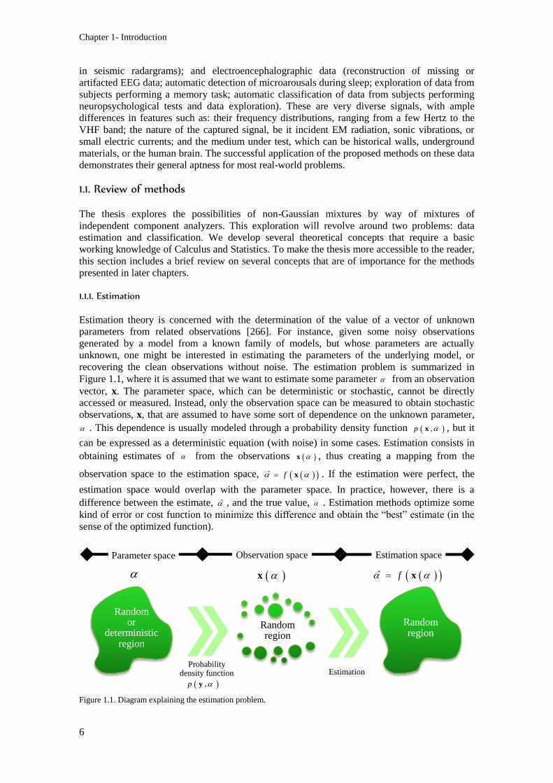
Chapter 1- Introduction
6
in seismic radargrams); and electroencephalographic data (reconstruction of missing or
artifacted EEG data; automatic detection of microarousals during sleep; exploration of data from
subjects performing a memory task; automatic classification of data from subjects performing
neuropsychological tests and data exploration). These are very diverse signals, with ample
differences in features such as: their frequency distributions, ranging from a few Hertz to the
VHF band; the nature of the captured signal, be it incident EM radiation, sonic vibrations, or
small electric currents; and the medium under test, which can be historical walls, underground
materials, or the human brain. The successful application of the proposed methods on these data
demonstrates their general aptness for most real-world problems.
1.1. Review of methods
The thesis explores the possibilities of non-Gaussian mixtures by way of mixtures of
independent component analyzers. This exploration will revolve around two problems: data
estimation and classification. We develop several theoretical concepts that require a basic
working knowledge of Calculus and Statistics. To make the thesis more accessible to the reader,
this section includes a brief review on several concepts that are of importance for the methods
presented in later chapters.
1.1.1. Estimation
Estimation theory is concerned with the determination of the value of a vector of unknown
parameters from related observations [266]. For instance, given some noisy observations
generated by a model from a known family of models, but whose parameters are actually
unknown, one might be interested in estimating the parameters of the underlying model, or
recovering the clean observations without noise. The estimation problem is summarized in
Figure 1.1, where it is assumed that we want to estimate some parameter from an observation
vector, x. The parameter space, which can be deterministic or stochastic, cannot be directly
accessed or measured. Instead, only the observation space can be measured to obtain stochastic
observations, x, that are assumed to have some sort of dependence on the unknown parameter,
. This dependence is usually modeled through a probability density function ,p x , but it
can be expressed as a deterministic equation (with noise) in some cases. Estimation consists in
obtaining estimates of from the observations x , thus creating a mapping from the
observation space to the estimation space, ˆ f x . If the estimation were perfect, the
estimation space would overlap with the parameter space. In practice, however, there is a
difference between the estimate, , and the true value, . Estimation methods optimize some
kind of error or cost function to minimize this difference and obtain the “best” estimate (in the
sense of the optimized function).
Figure 1.1. Diagram explaining the estimation problem.
Random region
Probability
density function Estimation
Parameter space Observation space Estimation space
Random region
Random or
deterministic region
,p y
x ˆ f x
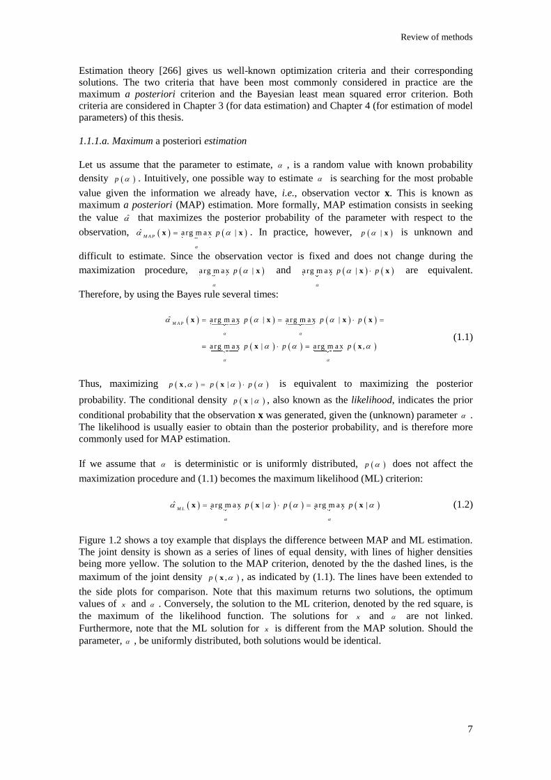
Review of methods
7
Estimation theory [266] gives us well-known optimization criteria and their corresponding
solutions. The two criteria that have been most commonly considered in practice are the
maximum a posteriori criterion and the Bayesian least mean squared error criterion. Both
criteria are considered in Chapter 3 (for data estimation) and Chapter 4 (for estimation of model
parameters) of this thesis.
1.1.1.a. Maximum a posteriori estimation
Let us assume that the parameter to estimate, , is a random value with known probability
density p . Intuitively, one possible way to estimate is searching for the most probable
value given the information we already have, i.e., observation vector x. This is known as
maximum a posteriori (MAP) estimation. More formally, MAP estimation consists in seeking
the value that maximizes the posterior probability of the parameter with respect to the
observation, ˆ arg m ax |M A P
p
x x . In practice, however, |p x is unknown and
difficult to estimate. Since the observation vector is fixed and does not change during the
maximization procedure, arg m ax |p
x and arg m ax |p p
x x are equivalent.
Therefore, by using the Bayes rule several times:
ˆ a rg m a x | a rg m a x |
a rg m a x | a rg m a x ,
M A Pp p p
p p p
x x x x
x x (1.1)
Thus, maximizing , |p p p x x is equivalent to maximizing the posterior
probability. The conditional density |p x , also known as the likelihood, indicates the prior
conditional probability that the observation x was generated, given the (unknown) parameter .
The likelihood is usually easier to obtain than the posterior probability, and is therefore more
commonly used for MAP estimation.
If we assume that is deterministic or is uniformly distributed, p does not affect the
maximization procedure and (1.1) becomes the maximum likelihood (ML) criterion:
ˆ arg m ax | arg m ax |M L
p p p
x x x (1.2)
Figure 1.2 shows a toy example that displays the difference between MAP and ML estimation.
The joint density is shown as a series of lines of equal density, with lines of higher densities
being more yellow. The solution to the MAP criterion, denoted by the the dashed lines, is the
maximum of the joint density ,p x , as indicated by (1.1). The lines have been extended to
the side plots for comparison. Note that this maximum returns two solutions, the optimum
values of x and . Conversely, the solution to the ML criterion, denoted by the red square, is
the maximum of the likelihood function. The solutions for x and are not linked.
Furthermore, note that the ML solution for x is different from the MAP solution. Should the
parameter, , be uniformly distributed, both solutions would be identical.
Chapter 1- Introduction
8
Figure 1.2. Comparison of the joint density of one-dimensional observations, x, with respect to a parameter α. The
concentrical ovals denote points of equal density, with higher PDF being more yellow. The plots on the side of the
joint density show the PDF of α and the likelihood of x for the most common value of α. Note that the maximum of
the joint density (denoted by the two dashed lines) yields a different solution than the maximum of the likelihood
function (denoted by the red square), particularly for x.
The MAP and ML criteria involve seeking the global maximum in a multidimensional function,
which can only be done by means of iterative algorithms like gradient methods. Hence,
problems of initialization and convergence to local maxima typically emerge in these solutions.
This has been considered in the applications of the ML criterion in this thesis in Chapter 3 and
Chapter 4.
1.1.1.b. Bayesian LMSE estimation
Another way to estimate the unknown parameter is by minimizing the “distance” between its
true value and the estimated value x , as defined by an cost (or cost) function ˆ, x .
Since and x are usually random variables, this error function is a random variable as
well. The Bayesian estimator is defined as the estimator that minimizes the average error
function of the estimate, ˆ,E
x . More explicitly, this average error function is:
ˆ ˆ, , ,
ˆ, |
E p d d
p p d d
x x x x
x x x x
(1.3)
The minimum average error can be obtained by setting the derivative of (1.3) to zero:
ˆ0 , ,ˆ
ˆ, |ˆ
dp d d
d
dp d p d
d
x x x
x x x x
(1.4.a)
ˆ0 , |ˆ
dp d
d
x x (1.4.b)
The solution to (1.4.b) depends on the shape of the error function, . In least mean squared
error estimation, the error function is set to the squared error: 2
ˆ ˆ, x x .
Substituting this error function in (1.4.b) results in
Den
sity
of
para
mete
r
Likelihood, p(x|)
Joint density p(,x)
ML estimation
MAP estimation
x
Review of methods
9
2
ˆ ˆ0 , | |ˆ ˆ
ˆ ˆ2 | 2 | 2 |
ˆ2 | 2
d dp d p d
d d
p d p d p d
p d
x x x x
x x x x x
x x
(1.5)
ˆ | |p d E x x x (1.6)
Thus, the solution to the LMSE criterion is the conditional expectation of the unknown
parameter with respect to the observation x.
In practice, the expectation cannot be formulated in closed form in most cases. Without a closed
form for |E x , the only way to solve (1.6) is through numerical methods such as Monte
Carlo numerical integration. In some cases, a solution can be obtained by finding a non-linear
function that can reasonably approximate the expectation. The simplest form of LMSE
estimation, however, is to assume that a linear approximation is sufficient, thus reaching the
solution of the linear LMSE (LLMSE) criterion. The advantage of the LLMSE criterion is that
the linear operator can be obtained by solving a system of linear equations (the Wiener-Hopf
equations [236]). Moreover, only second-order statistics are necessary to define this system.
When the model cannot be simplified by a linear approximation, however, the solution to the
LLMSE criterion is no longer optimal. This is demonstrated in Chapter 3 and Chapter 5, where
we compared our proposed ML and LMSE estimators with (among other methods) a classical
LLMSE estimator, Ordinary Kriging. The comparison is performed on sets of simulated
(Chapter 3) and real (Chapter 5) data.
1.1.2. Probability density estimation
The probability density is one of the main concepts in statistics. The probability density function
(PDF) p of a random variable x at value a, also written as xp x a or x
p a , is defined as the
likelihood that the random value takes the value a during any given realization. The PDF allows
to determine the probability of any realization of x falling within the interval [a, b]:
b
x
a
P a x b p x d x (1.7)
In practice, however, the probability density of the data is unknown. More typically, we have a
limited set of samples from some unknown density that we want to know. This is known as
probability density estimation. There are two main approaches to density estimation, parametric
estimation and non-parametric estimation. In parametric estimation, it is assumed that the data,
x, are drawn from a given density distribution or family of distributions (e.g., Gaussian or
Laplacian). The data are then used to estimate the parameters of the assumed distribution, e.g.,
the mean and standard deviation of the Gaussian distribution, or the mean and scale parameter
of the Laplacian distribution. Non-parametric estimation, on the other hand, assumes no explicit
distribution; only that the data follow some probability density function p . The data are used to
“build” a general probability density that can have almost any shape. There are many methods
for non-parametric density estimation, such as: histograms; naive estimator; nearest neighbors;
variable kernel; orthogonal series; maximum penalized likelihood; general weight function; and
bounded domains and directional data [75,244]. In this thesis, non-parametric kernel density
estimation (KDE) will be used. Thus, a brief review on KDE is included in this section.
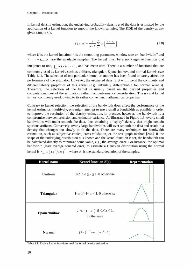
Chapter 1- Introduction
10
In kernel density estimation, the underlying probability density p of the data is estimated by the
application of a kernel function to smooth the known samples. The KDE of the density at any
given sample x is
1
1ˆ |
N
n
n
x xp x h K
N h h
(1.8)
where K is the kernel function; h is the smoothing parameter, window size or “bandwidth;” and
nx , 1, ...,n N are the available samples. The kernel must be a non-negative function that
integrates to one, 1K x d x
, and has mean zero. There is a number of functions that are
commonly used as kernels, such as uniform, triangular, Epanechnikov, and normal kernels (see
Table 1.1). The selection of one particular kernel or another has been found to barely affect the
performance of the estimator. However, the estimated density p will inherit the continuity and
differentiability properties of this kernel (e.g., infinitely differentiable for normal kernels).
Therefore, the selection of the kernel is usually based on the desired properties and
computational cost of the estimation, rather than performance consideration. The normal kernel
is most commonly used, owing to its rather convenient mathematical properties.
Contrary to kernel selection, the selection of the bandwidth does affect the performance of the
kernel estimator. Intuitively, one might attempt to use a small a bandwidth as possible in order
to improve the resolution of the density estimation. In practice, however, the bandwidth is a
compromise between precision and estimator variance. As illustrated in Figure 1.3, overly small
bandwidths will under-smooth the data, thus obtaining a “spiky” density that might contain
spurious artifacts. Conversely, overly large bandwidths will over-smooth the data and result in a
density that changes too slowly to fit the data. There are many techniques for bandwidth
estimation, such as subjective choice, cross-validation, or the test graph method [244]. If the
shape of the underlying distribution p is known and the kernel function is set, the bandwidth can
be calculated directly to minimize some value, e.g., the average error. For instance, the optimal
bandwidth (least average squared error) to estimate a Gaussian distribution using the normal
kernel is 1 / 5
5ˆ4 3
o p th N , where is the standard deviation of the samples.
Kernel name Kernel function K(x) Representation
Uniform 1/2 if -1≤ x ≤ 1, 0 otherwise
Triangular 1-|x| if -1≤ x ≤ 1, 0 otherwise
Epanechnikov
20 .7 5 1 x if -1≤ x ≤ 1,
0 otherwise
Normal 1 / 2 2
2 ex p / 2x
Table 1.1. Typical kernel functions used for kernel density estimation.
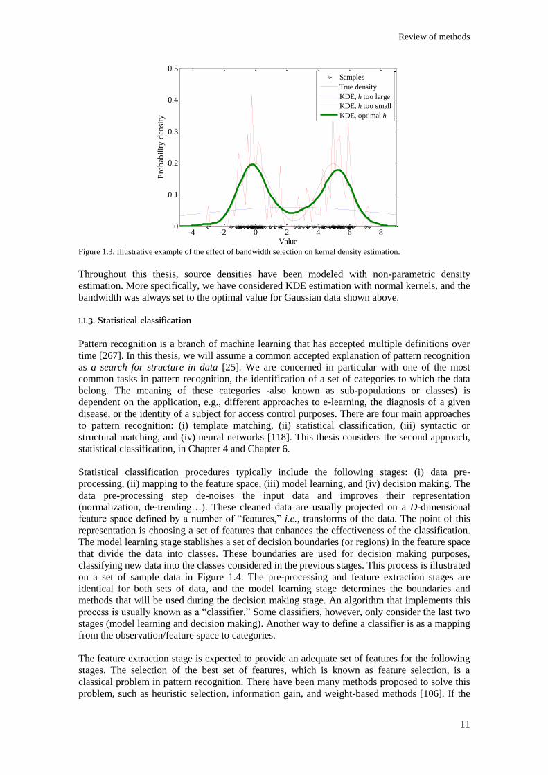
Review of methods
11
Figure 1.3. Illustrative example of the effect of bandwidth selection on kernel density estimation.
Throughout this thesis, source densities have been modeled with non-parametric density
estimation. More specifically, we have considered KDE estimation with normal kernels, and the
bandwidth was always set to the optimal value for Gaussian data shown above.
1.1.3. Statistical classification
Pattern recognition is a branch of machine learning that has accepted multiple definitions over
time [267]. In this thesis, we will assume a common accepted explanation of pattern recognition
as a search for structure in data [25]. We are concerned in particular with one of the most
common tasks in pattern recognition, the identification of a set of categories to which the data
belong. The meaning of these categories -also known as sub-populations or classes) is
dependent on the application, e.g., different approaches to e-learning, the diagnosis of a given
disease, or the identity of a subject for access control purposes. There are four main approaches
to pattern recognition: (i) template matching, (ii) statistical classification, (iii) syntactic or
structural matching, and (iv) neural networks [118]. This thesis considers the second approach,
statistical classification, in Chapter 4 and Chapter 6.
Statistical classification procedures typically include the following stages: (i) data pre-
processing, (ii) mapping to the feature space, (iii) model learning, and (iv) decision making. The
data pre-processing step de-noises the input data and improves their representation
(normalization, de-trending…). These cleaned data are usually projected on a D-dimensional
feature space defined by a number of “features,” i.e., transforms of the data. The point of this
representation is choosing a set of features that enhances the effectiveness of the classification.
The model learning stage stablishes a set of decision boundaries (or regions) in the feature space
that divide the data into classes. These boundaries are used for decision making purposes,
classifying new data into the classes considered in the previous stages. This process is illustrated
on a set of sample data in Figure 1.4. The pre-processing and feature extraction stages are
identical for both sets of data, and the model learning stage determines the boundaries and
methods that will be used during the decision making stage. An algorithm that implements this
process is usually known as a “classifier.” Some classifiers, however, only consider the last two
stages (model learning and decision making). Another way to define a classifier is as a mapping
from the observation/feature space to categories.
The feature extraction stage is expected to provide an adequate set of features for the following
stages. The selection of the best set of features, which is known as feature selection, is a
classical problem in pattern recognition. There have been many methods proposed to solve this
problem, such as heuristic selection, information gain, and weight-based methods [106]. If the
-4 -2 0 2 4 6 80
0.1
0.2
0.3
0.4
0.5
Value
Pro
bab
ilit
y d
ensi
ty
Samples
True density
KDE, h too large
KDE, h too small
KDE, optimal h
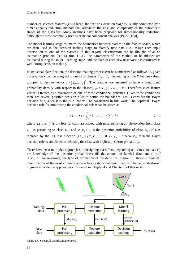
Chapter 1- Introduction
12
number of selected features (D) is large, the feature extraction stage is usually completed by a
dimensionality-reduction method that alleviates the cost and complexity of the subsequent
stages of the classifier. Many methods have been proposed for dimensionality reduction,
although the most commonly used is principal component analysis (PCA, [124]).
The model learning stage estimates the boundaries between classes in the feature space, which
are then used in the decision making stage to classify new data (i.e., assign each input
observation to one of the classes). In this regard, classification can be thought of as an
estimation problem (see Section 1.1.1): the parameters of the method or boundaries are
estimated during the model learning stage, and the class of each new observation is estimated as
well during decision making.
In statistical classification, the decision making process can be summarized as follows. A given
observation y can be assigned to one of K classes 1, ...,
KC C depending on the D feature values,
grouped in feature vector 1, ...,
T
Df ff . The features are assumed to have a conditional
probability density with respect to the classes, |k
p Cf , 1, ...,k K . Therefore, each feature
vector is treated as a realization of one of these conditional densities. Given these conditions,
there are several possible decision rules to define the boundaries. Let us consider the Bayes
decision rule, since it is the rule that will be considered in this work. The “optimal” Bayes
decision rule for minimizing the conditional risk R can be stated as
1
| , |
K
k k j j
j
R C L C C P C
f f (1.9)
where ,i j
L C C is the loss function associated with misclassifying an observation from class
jC as pertaining to class
iC , and |
kP C f is the posterior probability of class
kC . If L is
replaced by the 0/1 loss function (i.e., , 1i j
L C C if i j , 0 otherwise), then the Bayes
decision rule is simplified to selecting the class with highest posterior probability.
There have been multiples approaches to designing classifiers, depending on issues such as: (i)
the knowledge of the posterior probabilities; (ii) the amount of labeled data; and (iii) if
|k
P C f are unknown, the type of estimation of the densities. Figure 1.5 shows a classical
classification of the most common approaches to statistical classification. The boxes shadowed
in green indicate the approaches considered in Chapter 4 and Chapter 6 of this work.
Figure 1.4. Statistical classification process.
Training
data Pre-
processing Feature
extraction Model
learning
New
data Pre-
processing Feature
extraction Decision
making Classes
(identical) (identical) (model,
boundaries)
Class 2
Class 1
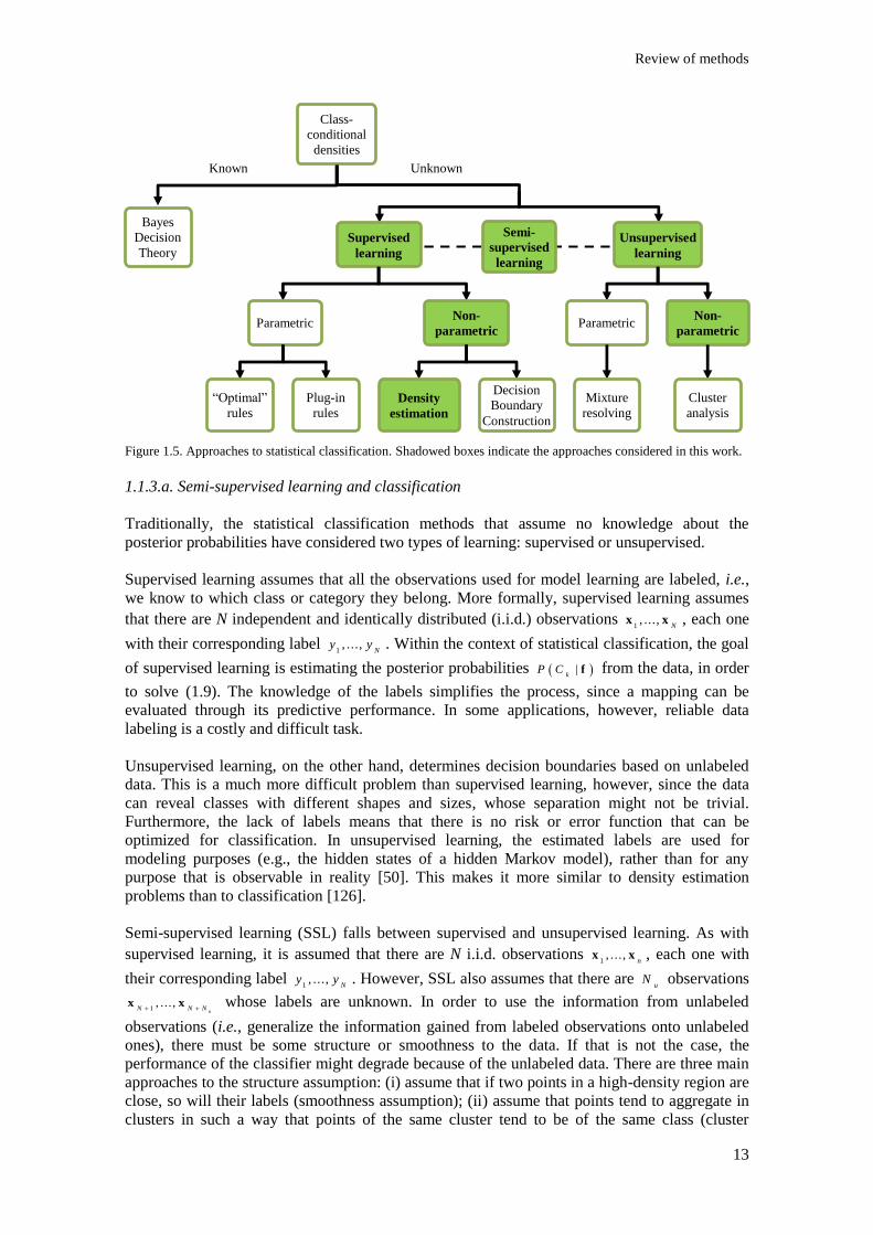
Review of methods
13
Figure 1.5. Approaches to statistical classification. Shadowed boxes indicate the approaches considered in this work.
1.1.3.a. Semi-supervised learning and classification
Traditionally, the statistical classification methods that assume no knowledge about the
posterior probabilities have considered two types of learning: supervised or unsupervised.
Supervised learning assumes that all the observations used for model learning are labeled, i.e.,
we know to which class or category they belong. More formally, supervised learning assumes
that there are N independent and identically distributed (i.i.d.) observations 1, ...,
Nx x , each one
with their corresponding label 1, ...,
Ny y . Within the context of statistical classification, the goal
of supervised learning is estimating the posterior probabilities |k
P C f from the data, in order
to solve (1.9). The knowledge of the labels simplifies the process, since a mapping can be
evaluated through its predictive performance. In some applications, however, reliable data
labeling is a costly and difficult task.
Unsupervised learning, on the other hand, determines decision boundaries based on unlabeled
data. This is a much more difficult problem than supervised learning, however, since the data
can reveal classes with different shapes and sizes, whose separation might not be trivial.
Furthermore, the lack of labels means that there is no risk or error function that can be
optimized for classification. In unsupervised learning, the estimated labels are used for
modeling purposes (e.g., the hidden states of a hidden Markov model), rather than for any
purpose that is observable in reality [50]. This makes it more similar to density estimation
problems than to classification [126].
Semi-supervised learning (SSL) falls between supervised and unsupervised learning. As with
supervised learning, it is assumed that there are N i.i.d. observations 1, ...,
nx x , each one with
their corresponding label 1, ...,
Ny y . However, SSL also assumes that there are
uN observations
1, . . . ,
uN N N
x x whose labels are unknown. In order to use the information from unlabeled
observations (i.e., generalize the information gained from labeled observations onto unlabeled
ones), there must be some structure or smoothness to the data. If that is not the case, the
performance of the classifier might degrade because of the unlabeled data. There are three main
approaches to the structure assumption: (i) assume that if two points in a high-density region are
close, so will their labels (smoothness assumption); (ii) assume that points tend to aggregate in
clusters in such a way that points of the same cluster tend to be of the same class (cluster
Class-
conditional
densities Known
Bayes
Decision
Theory
Unknown
Supervised
learning
Parametric
“Optimal”
rules Plug-in
rules
Non-
parametric
Density
estimation
Decision
Boundary
Construction
Unsupervised
learning
Parametric
Mixture
resolving
Non-
parametric
Cluster
analysis
Semi-
supervised
learning
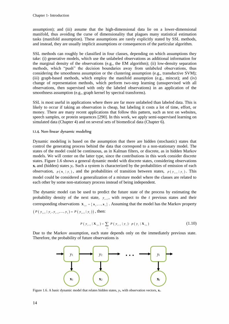
Chapter 1- Introduction
14
assumption); and (iii) assume that the high-dimensional data lie on a lower-dimensional
manifold, thus avoiding the curse of dimensionality that plagues many statistical estimation
tasks (manifold assumption). These assumptions are rarely explicitly stated by SSL methods,
and instead, they are usually implicit assumptions or consequences of the particular algorithm.
SSL methods can roughly be classified in four classes, depending on which assumptions they
take: (i) generative models, which use the unlabeled observations as additional information for
the marginal density of the observations (e.g., the EM algorithm); (ii) low-density separation
methods, which “push” the decision boundaries away from unlabeled observations, thus
considering the smoothness assumption or the clustering assumption (e.g., transductive SVM);
(iii) graph-based methods, which employ the manifold assumption (e.g., mincut); and (iv)
change of representation methods, which perform two-step learning (unsupervised with all
observations, then supervised with only the labeled observations) in an application of the
smoothness assumption (e.g., graph kernel by spectral transforms).
SSL is most useful in applications where there are far more unlabeled than labeled data. This is
likely to occur if taking an observation is cheap, but labeling it costs a lot of time, effort, or
money. There are many recent applications that follow this pattern, such as text on websites,
speech samples, or protein sequences [290]. In this work, we apply semi-supervised learning on
simulated data (Chapter 4) and on several sets of biomedical data (Chapter 6).
1.1.4. Non-linear dynamic modeling
Dynamic modeling is based on the assumption that there are hidden (stochastic) states that
control the generating process behind the data that correspond to a non-stationary model. The
states of the model could be continuous, as in Kalman filters, or discrete, as in hidden Markov
models. We will center on the latter type, since the contributions in this work consider discrete
states. Figure 1.6 shows a general dynamic model with discrete states, considering observations
xt and (hidden) states yt. Such a system is characterized by the probabilities of emission of each
observation, |t t
p yx , and the probabilities of transition between states, 1|
t tp y y
. This
model could be considered a generalization of a mixture model where the classes are related to
each other by some non-stationary process instead of being independent.
The dynamic model can be used to predict the future state of the process by estimating the
probability density of the next state, 1t
y
, with respect to the t previous states and their
corresponding observations 1: 1, . . . ,
t tX x x . Assuming that the model has the Markov property
1 1 1 1| , , ..., |
t t t t tP y y y y P y y
, then:
1 1: 1 1:| | |
t
t t t t t t
y
P y P y y p y
X X (1.10)
Due to the Markov assumption, each state depends only on the immediately previous state.
Therefore, the probability of future observations is
Figure 1.6. A basic dynamic model that relates hidden states, yt, with observation vectors, xt.
y1
x1
y2
x2
yt
xt
···

Scope
15
1
1 1: 1 1 1 1:, . . . , | , . . . , | |
t
t t k t t t k t t t
y
P p y P y
x x X x x X (1.11)
for any k > 0. Thus, calculating the probability of the observations at times t + 1 through t + k
does not require knowledge of the previous observations 1:t
X , but only of the state of the system
at time t. In order to incorporate higher order dependences, a representation of the form
1, , ...,
T
t t t t ky y y
Y can be considered. This expanded representation is considered throughout
Chapter 4 of this thesis, where we consider the dependences between multiple Markov chains.
The dynamics of the system (transition probabilities and probability densities of the
observations) can be used to implement linear or non-linear models. Linear models can be
estimated using techniques such as expectation maximization (EM). In particular, HMM are
most commonly estimated using the Baum-Welch algorithm [17], a particular implementation
of the EM algorithm for hidden Markov models. The Baum-Welch algorithm uses dynamic
programming to estimate the dynamics of the system in a fast manner. Nevertheless, system
dynamics cannot be approximated linearly in many real problems, thus motivating the inclusion
of non-linearities. There have been a number of approaches to non-linear dynamic models:
using probabilistic priors plus parametric models [207]; particle filtering using a finite number
of samples to represent the posterior distribution that are updated with new observation arrivals
[37]; and approximating the posterior 1:|
t tP y X by means of a mixture of distributions such
as mixture of Gaussians (MoG, also known as GMM) [53]. Recent works by the GTS have
proposed the use of non-Gaussian mixture models, using ICAMM in order to model the non-
linear part of the system dynamics [230]. Chapter 4 introduces a non-Gaussian mixture model
that is extended to consider multiple chains of dependence.
There is an extensive range of applications for hidden state-based dynamic models. The
objective is to exploit the sequential dependence of the data, which is inherent in many real-
world problems, in a scheme of sequential pattern recognition. Some of the applications of
HMM (the most common dynamic model) are the following: speech recognition [174], video
event classification and image segmentation [166], people recognition [167], and human motion
for robotics [145]. Of particular relevance is the application of HMM in event-related dynamics
of brain oscillations [183] and, in general, in causality analysis of physiological phenomena.
One example of these analyses is sleep staging, which is approached using radial basis function
(RBF) networks and HMM for the classification of EEG recordings measured during afternoon
naps in [139]. In Chapter 6, we address the sleep staging problem focusing on the analysis of
arousal provoked by apnea.
1.2. Scope
The scope of this work is the exploration of new possibilities of non-Gaussian mixtures. Thus,
new algorithms based on these mixtures will be designed for data estimation, feature extraction,
semi-supervised or unsupervised learning, and sequential dynamic modeling. The interpolation
algorithms will consider the use of non-Gaussian mixtures for the interpolation itself, unlike
other works where it was used as a pre-processing step. Two criterions will be considered for
this estimation: maximum likelihood and least mean square error. The modeling algorithms will
consider sequential dynamic modeling, which can in turn be used for unsupervised (or semi-
supervised) learning and feature extraction. The proposed methods will expand on previous
works and obtain general methods that combine several synchronized sets of data. The resulting
methods will be thoroughly explained using appropriate and demonstrative examples. Results
come from a large number of sets of synthetic and real data. Quantifiable evaluation will be
obtained for synthetic data where the underlying patterns and distributions are known.

Chapter 1- Introduction
16
In addition to its theoretical developments, this works intends to demonstrate the suitability of
the developed algorithms for real-world problems. The research carried out in this thesis is
framed within the following projects of the Grupo de Tratamiento de Señal of the Universitat
Politècnica de València:
“Técnicas Avanzadas de Procesado de Señales EEG para el Estudio de Estructuras de
Conectividad Cerebral,” supported by Generalitat Valenciana (Regional
Administration) under grant GV/2014/034.
“Clasificación de Señales Multimodales: Algoritmos y Aplicaciones,” supported by
Universitat Politècnica de València under grant SP20120646.
“Algoritmos para el Análisis de Modalidad de Señal: Aplicación en el Procesado
Avanzado de Señales Acústicas,” supported by the Spanish Administration under grant
TEC2011-23403.
“Procesador No-Lineal de Mezclas con Aplicación de Detección, Clasificación, Filtrado
y Predicción,” supported by the Spanish Administration under grant TEC2008-02975.
“Muros: Desarrollo de Metodologías No Destructivas de Aplicación a Muros
Históricos,” supported by IMPIVA and Universitat Politècnica de València under grant
IMIDIN/2008/7.
The aforementioned projects were concerned with developing software and applications for the
purposes of: (i) brain analysis and diagnosis on neurology patients; and (ii) characterization of
historical walls. In the first group, the non-Gaussian mixture techniques are used to detect
changes in the electroencephalographic signal captured during a battery of neuropsychological
tests. This system might be used to perform automatic diagnosis and evaluation of the subject’s
mental proficiency. In the second group of projects, the non-Gaussian mixtures are used to
reconstruct damaged data or estimate data at uncaptured positions, thus increasing the
capabilities of subsequent methods. Missing data is an important problem in several non-
destructive testing applications (e.g., in GPR [43]), and these techniques could help to improve
data.
1.3. Contributions
This thesis makes a number of contributions to the research in non-Gaussian mixtures. The three
main contributions are: two novel methods for data estimation based on ICA mixture models;
the introduction of a generalized model for sequential dependence in ICA mixture models; and
the introduction of ICA and ICA mixture models in diverse novel applications. These
applications are: reconstruction of damaged or missing ground-penetrating radar, reconstruction
of damaged or missing seismic data, reconstruction of artifacted or missing EEG data, diagnosis
of sleep disorders, and modeling of brain response during memory tasks. This work has inspired
several publications, including conference and journal papers and a book chapter (see the
publication list at the end of the thesis).
1.3.1. Interpolation based on ICA and ICA mixture models
Two novel methods based on ICA mixture models are proposed for the interpolation of missing
values in the observation record. Although ICA has been used for data interpolation
applications, it has been limited to the pre-processing stages of the interpolation process, to the
best of our knowledge (e.g., [164]). The methods proposed in this thesis, however, consider the
non-Gaussian mixture model as an integral part of the interpolation algorithm. These methods
were obtained by considering two commonly-used estimation criteria: (i) maximum likelihood;
(ii) least mean square error. The resulting methods were respectively named PREDICAMM
(Prediction using ICAMM) and E-ICAMM (Expectation assuming ICAMM), respectively.
PREDICAMM performs estimation by maximizing the conditional likelihood of the data to be
estimated, z, with respect to known data, y, and the model. In practice, this probability is
Contributions
17
replaced by the joint likelihood, ,p z y , which can be found from the ICAMM. The
maximization of any of these probabilities is equivalent and leads to the same solution (as
explained in Section 1.1.1.a). This maximization is performed using a gradient ascent method.
The resulting interpolation is robust with respect to the number of missing data in z, although
the initial point of the gradient must be selected carefully.
The second method, E-ICAMM, estimates missing data by minimizing the mean square error of
the interpolation. This is done by calculating the optimal solution for this case, the conditional
expectation of unknown data with respect to known data, E z | y . Given the ICA mixture
model, a closed-form solution can be obtained for this conditional expectation. The method is
relatively fast and the solution is robust with respect to the number of missing data in z.
Furthermore, since both methods make the same assumptions and consider the same model, E-
ICAMM can be used to obtain a starting point for the gradient step in PREDICAMM.
1.3.2. Sequential dynamic modeling
Previous works have presented a method that extends non-Gaussian mixtures to consider
sequential dependence, SICAMM (Sequential ICAMM, [230]). This method consists of a
sequential Bayes processor formulated from HMM theory, in which the ICAMM parameters
and the class transition probabilities are used for classification. This thesis extends the method
to consider several Markov chains in a coupled Hidden Markov model, with each class
considering a (potentially different) ICA mixture model. This allows for greater generalization
capabilities and the possibility to process multimodal data. We have named the resulting model
G-SICAMM (Generalized SICAMM). Furthermore, we adapt two classical HMM classification
algorithms, Baum-Welch [17] and Viterbi [270], for use with G-SICAMM.
Furthermore, this thesis presents a method for semi-supervised or unsupervised learning of the
G-SICAMM parameters, which we have named UG-SICAMM. This allows estimating the
model parameters using unlabeled data. Semi-supervised learning has been extensively studied
for different classification frameworks and classical generative models such as transductive
support vector machines, graph-based methods, hidden Markov random fields and Bayesian
classifiers [50], and in the context of information-theoretic learning [121,77].
1.3.3. New applications of ICA and ICAMM
The contributions described in Section 1.3.1 and 1.3.2 are general-purpose, and therefore, can
be applied to a wide range of applications. The design of an accurate model to “explain” a real
physical phenomenon is a complex work. Indeed, such a work could become the focus of a
thesis by and of itself. With this work, however, we intended to explore the possibilities of the
extensions of non-Gaussian mixtures in several different fields. Thus, we have applied the
developed methods to five real-world applications. The novelty and usefulness of the explored
applications are guaranteed since they arise from the development of research and engineering
projects (see Section 1.2). The contributions of this thesis for these real-world problems are
explained below.
1.3.3.a. Reconstruction of data from a GPR survey of historical walls
In ground-penetrating radar surveys, the GPR device emits high-frequency waves into the
medium under test at different locations and captures the reflections produced by discontinuities
in the material (e.g., air-to-material interfaces) [68]. The resulting data form a B-Scan or
radargram. The problem considered is the reconstruction of missing traces from the GPR B-
Scan. Missing traces are a classical problem in GPR, and can occur for a number of reasons
[68]. For this purpose, the B-Scan is transformed into a low-dimensional signal by pre-
processing and an ICA mixture model is obtained. Then, E-ICAMM and PREDICAMM are

Chapter 1- Introduction
18
used to reconstruct the missing data in the radargram. This contribution presents the first
application of ICAMM to the reconstruction of GPR data.
1.3.3.b. Reconstruction of seismic data from a seismic exploration survey
Seismic exploration is somewhat similar to GPR exploration. A typical reflection seismology
survey, however, has a single source event or “shot” that emits low-frequency waves. Once the
shot is generated, the reflections are then captured at the surface by groups of receivers,
resulting in a B-Scan or seismogram [241]. The problem considered is the reconstruction of
missing traces from the seismogram. Missing traces are a classical problem in seismic
exploration, chiefly due to the large distances involved and the hostile terrain [241]. For this
purpose, the B-Scan is transformed into a low-dimensional signal by pre-processing and an ICA
mixture model is obtained. Then, E-ICAMM and PREDICAMM are used to reconstruct the
missing data in the seismogram. This contribution presents the first application of ICAMM to
the reconstruction of seismic data.
1.3.3.c. Reconstruction of EEG data
The problem in this application is the reconstruction of missing values from EEG data from
subjects performing the Sternberg memory task. This can be used to reconstruct missing or
artifacted data. ICA methods have been used in many applications on EEG data, such as
removing artifacts [127]. However, the contributions of this thesis are unique in both the use of
an ICA mixture model and the way in which the data are recovered. Results show the potential
of E-ICAMM and PREDICAMM for the interpolation of EEG data. Furthermore, both methods
show a large robustness with respect to the number of missing data, and can correctly
interpolate a large number of missing or artifacted EEG channels at once.
1.3.3.d. Diagnosis of microarousals in sleeping subjects
The problem in this application is the detection of microarousals that occur during sleep due to
apneas. The data consist of processing features extracted from 8-hour EEG signals from several
subjects to estimate a two-class (wake-sleep) hypnogram. This work was initiated in [230,225],
but this thesis extends previous works by considering several subjects and the contributions
considered in Section 1.3.2. Results show the potential application of G-SICAMM for the
implementation of an automatic classifier of EEG data from sleeping subjects. A more accurate
detection of microarousals in the hypnogram will help to the medical diagnosis of sleep
disorders [225].
1.3.3.e. Analysis of the brain memory function
This application introduces the use of the sequential dependence model in G-SICAMM to
model the dynamic behavior of EEG signals during memory tasks. Aside from the contributions
commented in Section 1.3.3.c, G-SICAMM is used to separate the data into two states
(stimulus-answer) during each one of a battery of neuropsychological tests. The methods are
tested on real data from several subjects, and they are shown to differentiate well between the
two suggested states for all tests. In addition, the parameters of G-SICAMM show activations of
several brain regions in consistence with the expected activations due to the neuropsychological
tests. Therefore, it is proven that the estimated G-SICAMM parameters are able to determine
brain connectivity patterns.

Overview
19
1.4. Overview
This thesis comprises seven chapters. Broadly speaking, they can be divided into introduction
(Chapter 1), background (Chapter 2), theoretical contributions (Chapters 3 and 4), applications
to real data (Chapters 5 and 6), and conclusions (Chapter 7). Chapter 2 deals with the theoretical
foundations of non-Gaussian mixture processing methods. Since this work expands on the
possible applications of these mixture models, a review of many different types of models is
presented in this chapter. Some of the methods presented in this chapter are then compared with
the methods proposed in this thesis.
The theoretical contributions of this thesis can be split into two categories, interpolation
algorithms (Chapter 3) and dynamic modeling methods (Chapter 4). Chapter 3 introduces two
novel non-linear interpolation methods that are based on ICA mixture models, named
PREDICAMM and E-ICAMM. In ICAMM, observations are partitioned into several mutually-
exclusive classes, each one modeled by a different ICA model. This underlying model is used to
interpolate unknown (or missing) values of the observation vector from the remaining known
values of the same vector. Each of the proposed interpolation methods approached this problem
in a different way. PREDICAMM seeks the maximum likelihood criterion, i.e., the
reconstruction that maximizes the conditional probability density of unknown data with respect
to known data. E-ICAMM, on the other hand, seeks the least mean square error criterion, i.e.,
minimizing the mean squared error of the reconstruction. Both methods are tested with an
extensive set of experiments. These experiments consider their performance on data generated
by an ICAMM, but also the reduction or alteration in performance incurred by any alterations of
this underlying model. Results are discussed and compared with those of other interpolation
methods, both classical and state-of-the-art.
Chapter 4 describes two new procedures for dynamic non-Gaussian modeling which are based
on synchronized ICAMM. The starting point of this work is SICAMM, a method that
incorporated a hidden Markov model to extend ICAMM to consider sequential dependence in
the observations [230]. The proposed methods in this chapter extend the one Markov chain
featured in SICAMM to a general framework to characterize the joint behavior of a number of
synchronized dynamic models or “chains.” We have named these methods G-SICAMM and
UG-SICAMM. The latter maximizes the log-likelihood of the model with respect to all of the
available training data and the parameters of the model, and can work with unsupervised or
semi-supervised data. The methods are validated using several experiments on simulated data.
These experiments consider both stationary and dynamically-changing data, thus testing the
limitations of the proposed methods and performing sensitivity analysis. Results are discussed
and compared with those of a commonly-used modeling method, Bayesian networks.
The methods developed in Chapters 3 and 4 are considered for real applications in Chapters 5
and 6, respectively. Chapter 5 shows the application of E-ICAMM and PREDICAMM for
reconstruction of three types of data. The first application is based on non-destructive testing
signals from ground-penetrating radar experiments. These signals are usually B-Scans, so they
are first converted to low-dimensional signals using a process common in applications of ICA to
image processing (e.g., [111]). The performance of the proposed methods is tested on simulated
data and on real GPR data from a survey on replicas of historical walls, and compared with that
of Kriging, Wiener structures, and splines. The second application considers the reconstruction
of seismic data from a reflection seismology survey. These signals are somewhat similar to
GPR, but they are more complex because they cover a larger area and the terrain is more hostile.
As with GPR, the signals are converted to low-dimensional signals and then used for the
interpolation experiment. The performance of E-ICAMM and PREDICAMM is compared with
that of Kriging, Wiener structures and splines. In the third application, the proposed methods are
used to reconstruct missing data from an electroencephalogram, a recording of the brain
electrical activity on the scalp. The EEG were captured from subjects that were performing the
Sternberg memory task. The proposed methods were compared with spherical splines, a

Chapter 1- Introduction
20
commonly-used method for interpolating EEG data. In all three applications, E-ICAMM and
PREDICAMM outperform the methods with which they are compared. Furthermore, it is shown
that both methods are highly resistant with respect to the number of missing data, and can
perform well even if a high number of values are missing from each observation.
Chapter 6 includes three applications of the methods developed in Chapter 4 to the modeling of
real EEG data. The first application considers the use of dynamic models for detection of
microarousals caused by apneas during sleep. These abrupt changes are registered in a diagram
known as “hypnogram,” which shows the different sleep stages during the night. Long EEG
records from apnea patients are analyzed, with the intention of detecting microarousals. The
classification obtained by the proposed methods outperforms that of dynamic Bayesian
networks. The second application analyzes EEG data taken from subjects performing the
Sternberg memory task. The proposed methods are used to model the transitions in the EEG
during the stages of the experiment. Results show the sensitivity of the G-SICAMM parameters
to the stages of the experiment, which allow for accurate detection. The third application
considers EEG data taken from epilepsy patients during a battery of neuropsychological tests.
The proposed methods are used to differentiate EEG taken during stimulus presentation from
data taken during the responses of the subjects. The methods from Chapter 4 are shown to over-
perform dynamic Bayesian networks for this task. Furthermore, the G-SICAMM parameters are
used to model the EEG and analyze the behavior of the brain during these experiments.
Chapter 7 completes the thesis with the conclusions and findings, as well as discussion of the
remaining open questions and future directions of research.
Finite mixture models with non-Gaussian components 2

23
- Finite mixture models with non-Gaussian components
2.1. Introduction
This chapter presents theoretical foundations on data modeling using finite mixture models
(FMM) of non-Gaussian distributions. Particularly, the independent component analysis mixture
model that is used in the developments of this work is reviewed in detail. A FMM is a convex
combination of two or more probability density functions. Thus, the combination of the
individual PDF properties allows for the approximation of arbitrary distributions. FMM has
been used in many fields of statistical analysis and machine learning such as modeling,
clustering, and classification. There exists an extensive literature of FMM and its applications
from the first known work in modern statistical literature [184] until today [170,88,171]. The
flexibility of using different kinds of basic PDFs makes FMM suitable for modeling the
geometry of complex data. A mixture model is able to model quite different complex
distributions through an appropriate choice of its components to accurately represent the local
areas of the true distribution. It can handle situations where a single parametric family is unable
to provide a satisfactory model for local variations in the observed data. Depending on the
application field, the geometry of the data can be defined using one (univariate) or several
(multivariate) random variables.
Briefly, let 1, . . . ,
LX X X be an L–dimensional continuous random variable and 1
, ,T
Lx xx
be an observation vector of X, where T means transposition. The PDF of a mixture model is
defined by a convex combination of K component PDFs [170],
1
|
K
k k k k
k
p p
x | Θ x θ (2.1)
where kp x | Θ is the PDF of the k -th component,
k is the corresponding mixing proportion
(or component prior), and 1 1, ..., , , ...,
T
K K Θ is the vector of set of parameters. We
assume that 0k
, for 1, ...,k K , and 1
1
K
k
k
. By the property of convexity, given that
each |k k
p x θ defines a PDF, |p x Θ will also be a PDF.
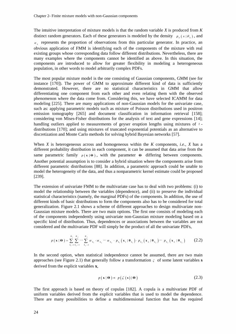
Chapter 2- Finite mixture models with non-Gaussian components
24
The intuitive interpretation of mixture models is that the random variable X is produced from K
distinct random generators. Each of these generators is modeled by the density |k k
p x , and
k represents the proportion of observations from this particular generator. In practice, an
obvious application of FMM is identifying each of the components of the mixture with real
existing groups whose corresponding data follow different distributions. Nevertheless, there are
many examples where the components cannot be identified as above. In this situation, the
components are introduced to allow for greater flexibility in modeling a heterogeneous
population, in other words to model arbitrarily complex PDFs.
The most popular mixture model is the one consisting of Gaussian components, GMM (see for
instance [170]). The power of GMM to approximate different kind of data is sufficiently
demonstrated. However, there are no statistical characteristics in GMM that allow
differentiating one component from each other and even relating them with the observed
phenomenon where the data come from. Considering this, we have selected ICAMM for data
modeling [225]. There are many applications of non-Gaussian models for the univariate case,
such as: applying parametric models such as mixture of Poisson distributions used in positron
emission tomography [265] and document classification in information retrieval [158];
considering von Mises-Fisher distributions for the analysis of text and gene expressions [14];
handling outliers applied to measurements of geyser eruption lengths using mixtures of t -
distributions [170]; and using mixtures of truncated exponential potentials as an alternative to
discretization and Monte Carlo methods for solving hybrid Bayesian networks [57].
When X is heterogeneous across and homogeneous within the K components, i.e., X has a
different probability distribution in each component, it can be assumed that data arise from the
same parametric family p x | Θ , with the parameter Θ differing between components.
Another potential assumption is to consider a hybrid situation where the components arise from
different parametric distributions [88]. In addition, a parametric approach could be unable to
model the heterogeneity of the data, and thus a nonparametric kernel estimate could be proposed
[239].
The extension of univariate FMM to the multivariate case has to deal with two problems: (i) to
model the relationship between the variables (dependence), and (ii) to preserve the individual
statistical characteristics (namely, the marginal PDFs) of the components. In addition, the use of
different kinds of basic distributions to form the components also has to be considered for total
generalization. Figure 2.1 shows a scheme of different approaches to design multivariate non-
Gaussian mixture models. There are two main options. The first one consists of modeling each
of the components independently using univariate non-Gaussian mixture modeling based on a
specific kind of distribution. Thus, dependences or associations between the variables are not
considered and the multivariate PDF will simply be the product of all the univariate PDFs,
1 2
1 2 1 1 2 2
1 2
1 2
1 1 1
| | | |
L
L L L
L
K K K
k k k k k k k k L k
k k k
p p p p
x Θ x θ x θ x θ (2.2)
In the second option, when statistical independence cannot be assumed, there are two main
approaches (see Figure 2.1) that generally follow a transformation of some latent variables s
derived from the explicit variables x,
| |p p x Θ s Θ (2.3)
The first approach is based on theory of copulas [182]. A copula is a multivariate PDF of
uniform variables derived from the explicit variables that is used to model the dependence.
There are many possibilities to define a multidimensional function that has the required
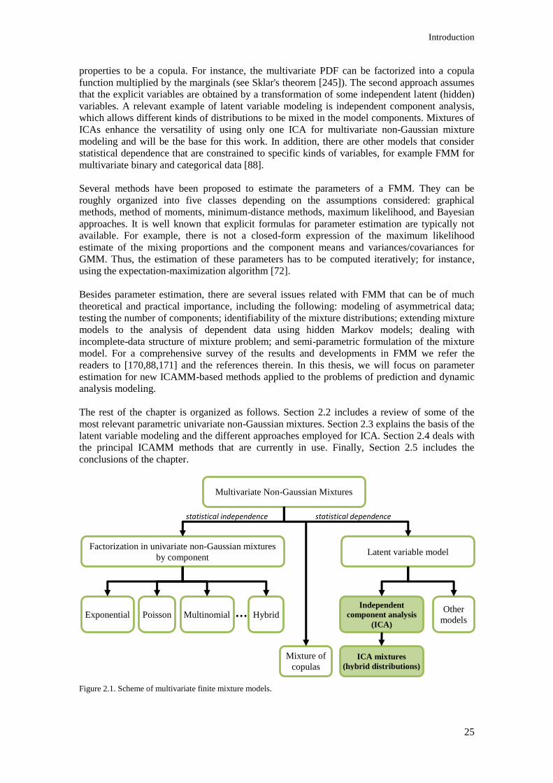
Introduction
25
properties to be a copula. For instance, the multivariate PDF can be factorized into a copula
function multiplied by the marginals (see Sklar's theorem [245]). The second approach assumes
that the explicit variables are obtained by a transformation of some independent latent (hidden)
variables. A relevant example of latent variable modeling is independent component analysis,
which allows different kinds of distributions to be mixed in the model components. Mixtures of
ICAs enhance the versatility of using only one ICA for multivariate non-Gaussian mixture
modeling and will be the base for this work. In addition, there are other models that consider
statistical dependence that are constrained to specific kinds of variables, for example FMM for
multivariate binary and categorical data [88].
Several methods have been proposed to estimate the parameters of a FMM. They can be
roughly organized into five classes depending on the assumptions considered: graphical
methods, method of moments, minimum-distance methods, maximum likelihood, and Bayesian
approaches. It is well known that explicit formulas for parameter estimation are typically not
available. For example, there is not a closed-form expression of the maximum likelihood
estimate of the mixing proportions and the component means and variances/covariances for
GMM. Thus, the estimation of these parameters has to be computed iteratively; for instance,
using the expectation-maximization algorithm [72].
Besides parameter estimation, there are several issues related with FMM that can be of much
theoretical and practical importance, including the following: modeling of asymmetrical data;
testing the number of components; identifiability of the mixture distributions; extending mixture
models to the analysis of dependent data using hidden Markov models; dealing with
incomplete-data structure of mixture problem; and semi-parametric formulation of the mixture
model. For a comprehensive survey of the results and developments in FMM we refer the
readers to [170,88,171] and the references therein. In this thesis, we will focus on parameter
estimation for new ICAMM-based methods applied to the problems of prediction and dynamic
analysis modeling.
The rest of the chapter is organized as follows. Section 2.2 includes a review of some of the
most relevant parametric univariate non-Gaussian mixtures. Section 2.3 explains the basis of the
latent variable modeling and the different approaches employed for ICA. Section 2.4 deals with
the principal ICAMM methods that are currently in use. Finally, Section 2.5 includes the
conclusions of the chapter.
Figure 2.1. Scheme of multivariate finite mixture models.
Multivariate Non-Gaussian Mixtures
Factorization in univariate non-Gaussian mixtures
by component Latent variable model
Exponential Poisson Multinomial … Independent
component analysis
(ICA)
Other
models
ICA mixtures
(hybrid distributions)
Hybrid
statistical independence statistical dependence
Mixture of
copulas
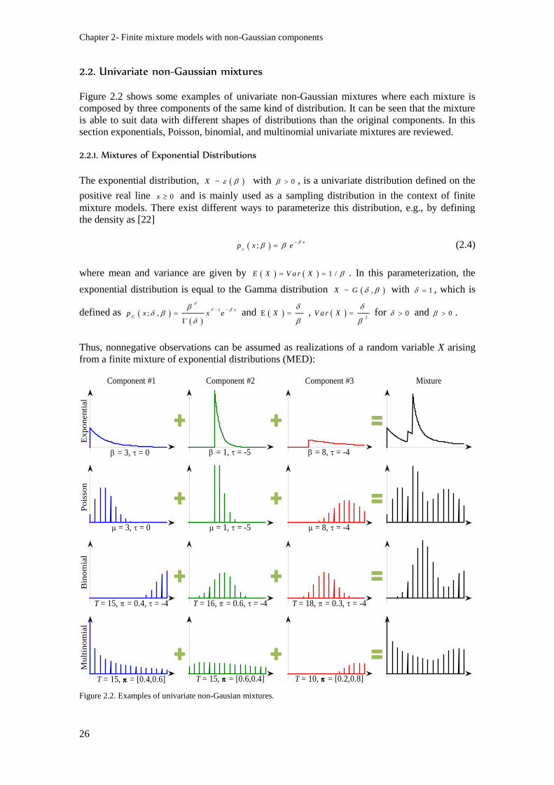
Chapter 2- Finite mixture models with non-Gaussian components
26
2.2. Univariate non-Gaussian mixtures
Figure 2.2 shows some examples of univariate non-Gaussian mixtures where each mixture is
composed by three components of the same kind of distribution. It can be seen that the mixture
is able to suit data with different shapes of distributions than the original components. In this
section exponentials, Poisson, binomial, and multinomial univariate mixtures are reviewed.
2.2.1. Mixtures of Exponential Distributions
The exponential distribution, ~X with 0 , is a univariate distribution defined on the
positive real line 0x and is mainly used as a sampling distribution in the context of finite
mixture models. There exist different ways to parameterize this distribution, e.g., by defining
the density as [22]
;x
p x e
(2.4)
where mean and variance are given by 1 /E X V a r X . In this parameterization, the
exponential distribution is equal to the Gamma distribution ~ ,X G with 1 , which is
defined as
1; ,
x
Gp x x e
and E X
,
2V a r X
for 0 and 0 .
Thus, nonnegative observations can be assumed as realizations of a random variable X arising
from a finite mixture of exponential distributions (MED):
Figure 2.2. Examples of univariate non-Gausian mixtures.
= 3, = 0
Ex
po
nen
tial
Component #1
= 1, = -5
Component #2
= 8, = -4
Component #3 Mixture
= 3, = 0
Po
isso
n
= 1, = -5 = 8, = -4
T = 15, = 0.4, = -4
Bin
om
ial
T = 16, = 0.6, = -4 T = 18, = 0.3, = -4
T = 15, = [0.4,0.6]
Mu
ltin
om
ial
T = 15, = [0.6,0.4] T = 10, = [0.2,0.8]
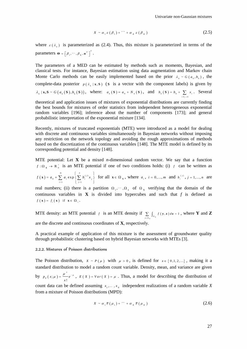
Univariate non-Gaussian mixtures
27
1 1~
K KX (2.5)
where k is parameterized as (2.4). Thus, this mixture is parameterized in terms of the
parameters 1, , ,
TT
K
Θ α .
The parameters of a MED can be estimated by methods such as moments, Bayesian, and
classical tests. For instance, Bayesian estimation using data augmentation and Markov chain
Monte Carlo methods can be easily implemented based on the prior 0 0~ ,
kG a b , the
complete-data posterior | ,k
p x S ( S is a vector with the component labels) is given by
| ~ ,k k k
G a b x, S S S , where: 0k ka a N S S , and 0
:i
k i
i S k
b b x
S . Several
theoretical and application issues of mixtures of exponential distributions are currently finding
the best bounds for mixtures of order statistics from independent heterogeneous exponential
random variables [196]; inference about the number of components [173]; and general
probabilistic interpretation of the exponential mixture [134].
Recently, mixtures of truncated exponentials (MTE) were introduced as a model for dealing
with discrete and continuous variables simultaneously in Bayesian networks without imposing
any restriction on the network topology and avoiding the rough approximations of methods
based on the discretization of the continuous variables [148]. The MTE model is defined by its
corresponding potential and density [148].
MTE potential: Let X be a mixed n-dimensional random vector. We say that a function
0: Rf
X is an MTE potential if one of two conditions holds: (i) f can be written as
( )
0
1 1
ex p
m n
j
i i j
i j
f a a b x
x for all
Xx , where
ia , 0, ...,i m and j
ib , 1, ...,j n are
real numbers; (ii) there is a partition 1, ,
k of
X verifying that the domain of the
continuous variables in X is divided into hypercubes and such that f is defined as
i f i i
f f x x x .
MTE density: an MTE potential f is an MTE density if , 1
y
f d
Z
Y
y z z , where Y and Z
are the discrete and continuous coordinates of X, respectively.
A practical example of application of this mixture is the assessment of groundwater quality
through probabilistic clustering based on hybrid Bayesian networks with MTEs [3].
2.2.2. Mixtures of Poisson distributions
The Poisson distribution, ~X P with 0 , is defined for 0 ,1, 2 , . . .x , making it a
standard distribution to model a random count variable. Density, mean, and variance are given
by ;!
x
p x ex
, E X V a r X . Thus, a model for describing the distribution of
count data can be defined assuming 1, ,
Nx x independent realizations of a random variable X
from a mixture of Poisson distributions (MPD):
1 1~
K KX (2.6)
Chapter 2- Finite mixture models with non-Gaussian components
28
This mixture is parameterized in terms of 2 1K distinct model parameters
1, ..., ,
TT
K
Θ α . For an MPD is easy to verify that the complete-data maximum likelihood
estimator of k
is equal to the sample mean in group k , ˆk k
x S , under the assumption that
the allocations (group indicators, variables that take values in the set 1, ..., K ) 1, ...,
T
NS SS
are observed as well. The complete-data ML estimator lies in the interior of the parameter
space, if each group is nonempty 0k
N S and contains at least one nonzero observation.
Asymptotic 95% confidence intervals for k
are equal to 1 .96 /k k k
x x NS S S , where
the expected Fischer information has been evaluated at k kx S . The effective coverage
probability may be considerable smaller, if the sample size N and the true values of k
and k
are very small where asymptotic 95% confidence intervals are compared with Bayesian
confidence intervals. Also the parameters of a MPD can be estimated by moments, data
augmentation and Markov chain Monte Carlo, and distance-based methods.
The applications of MPDs include quite different issues such as counts of fish species abundant
in a lake [237] and representation of protein abundance levels [141].
2.2.3. Mixtures of binomial distributions
For binomial mixtures, the component densities arise from ,B iN o m T distributions, where
T is commonly assumed to be known, whereas the component-specific probabilities are
unknown and heterogeneous:
1 1~ , ... ,
K KX B iN o m T B iN o m T (2.7)
The density of this mixture is given by
1
| 1
KT xx
k k k
k
Tp x
x
Θ (2.8)
with 1, ..., ,
TT
K
Θ α . Mixtures of binomial distributions (MBD) are not necessarily
identifiable; a necessary and sufficient condition is 2 1T K . MBD may be extended to the
case where i
T varies between the realizations 1, ...,
Nx x as follows:
1
| 1i ii
KT xi y
i k k k
k i
Tp x
x
Θ (2.9)
Bayesian inference for MBD is considered in [33] by applying a Metropolis-Hastings algorithm.
Bayesian estimation using data augmentation and Markov chain Monte Carlo can be
implemented to estimate an MBD by using the conjugate Beta prior ~ ,k k k
B a b S S , and
the posterior |k
p x , S is again a Beta distribution, | ~ ,k k k
B a b x, S S S , where
0
:i
k i
i S k
a a x
S , 0
:i
k i
i S k
b b T x
S .
MBD has been applied to problems involving binary data, e.g., estimating the trend of extreme
weather from rain data using a global climate model [38] and improving aquatic warbler
population assessment by accounting for imperfect detection [191].
Multivariate non-Gaussian
29
2.2.4. Mixtures of multinomial distributions
Consider a categorical variable of more than two categories 1, .. . , D . Let l
X , for 1, ..,l D , be
the number of occurrences of category l among T trials. If the occurrence probability
distribution 1, ...,
T
D π of each category is homogeneous among the observed data vectors,
then
1, . . . , ~ ,
DX X M u lN o m TX π (2.10)
To deal with unobserved heterogeneity in the occurrence probability of the various categories,
1, . . . ,
DX XX can be assumed to follow a finite mixture of multinomial distributions (MMD),
1 1~ M u lN o m , M u lN o m ,
K KX T T π π (2.11)
with ,1 ,
, ...,T
k k k D
π being the unknown occurrence probability in group k . The density is
given by
,
1 11
| l
DK
x
k k l
k lD
Tp
x Θ (2.12)
where 1
, ..., ,T
T T T
K
Θ π π α are the parameters of the mixture.
Bayesian estimation of the MMD parameters can be implemented based on the Dirichlet prior
0 ,1 0 ,~ , ...,
k DD a aπ , and the posterior |
kp π x , S is again a Dirichlet distribution
0 ,1 0 ,| ~ , ...,
k DD a aπ x, S S S , where , 0 ,
:i
k l l i l
i S k
a a x
S , 1, ...,l D .
Some of the recent applications of MMD include the following: learning multinomial mixture
models for text document classification based on the large margin criterion [122] and solving
the problem of age-invariant face recognition [29].
2.3. Multivariate non-Gaussian
In this section, the main definitions and applications of the copula method and latent variable
modeling are reviewed. These techniques are flexible tools for PDF modeling. They allow both
independence and dependence among variables to be jointly modeled for multivariate non-
Gaussian distribution mixtures. In particular, the principles of the LVM method called
independent component analysis are explained and discussed, since they will be used to derive
the theoretical contributions of this thesis.
2.3.1. Copula functions
The first reference to copula functions is included in [245] as a link between multidimensional
PDFs and marginal PDFs. The copula represents multivariate PDFs whose univariate marginal
PDFs are uniform in the interval [0, 1]. Copula functions can be used to describe the
dependence between random variables, i.e., the manner in which the variables covariate. The
marginal PDFs describe the behaviour of each of the components separately and the copula
function describes the dependence structure among these components. Several kinds of copulas
are defined in the literature to describe different kind of dependence [165]. The copulas have

Chapter 2- Finite mixture models with non-Gaussian components
30
been extensively used in the field of econometrics and finance (see [203] and the references
therein), and there are also a few applications in signal processing [117,256,254].
The copula function is defined by Sklar's theorem [245] considering the following. The joint
probability distribution 1 2, , . . . ,
DF x x x of a number of random variables
1 2, , ...,
DX X X can be
expressed from the marginal probability distributions associated to each of the random variables
i iF x , 1, ...,i D , as follows:
1 2 , 1 1 2 2 1, , , , , , , ,
D D D DF x x x C F x F x F x C U U (2.13)
By applying the probability integral transform to each original variable, uniformly distributed
marginals 1, . . . ,
DU U are obtained, which are random variables with components
iu defined as
i i iu F x , where
iF is the probability distribution function of
ix .
The function C is termed the copula function, which is a joint PDF of uniformly distributed
random variables in the interval [0, 1]. Thus, the copula function is defined in the unitary cube
: 0 1 0 1D
C U . The details of this theorem and the properties of copula functions can be
found in [245,203].
If the copula function C and the marginal distributions i
F are sufficiently differentiable, the
joint multivariate PDF can be obtained as the product of the marginals i
f (independence) and
the copula function of density c (dependence) derived from C . For continuous distributions, the
joint PDF is obtained as
1 2 1 1 2 2 1 1 2 2
in d ep en d en ce (m arg in a l d is trib u tio n s ) d ep en d en ce (co p u la fu n c tio n )
co m p lem en ta ry in fo rm a tio n co m m o n in fo rm a tio n
, , , , , ,D D D D D
f x x x f x f x f x c F x F x F x (2.14)
where 1 2
1 2
, , ,
, ,
D
D
D
C u u uc
u u u
u , i i i
u F x . The copula function of density c , in this
case, is a PDF of uniformly distributed random variables. If the random variables were
independent, the joint PDF would be the product of the marginal densities:
1 2
1
, , ,
D
D i iin d e p e n d e n t
i
f z z z f z
.
In order to parameterize the joint PDF defined as in (2.14), we have to find two sets of
parameters, those related with the marginals and those related with the copula function (the
parameters that model the dependence):
1 2 1 1 2 2 2
1
, , , | ; / , / , , / /
D
D i i i i D D D
i
f x x x f c F x F x F x
Θ x φ φ φ φ Λ (2.15)
Thus, the multivariate model is parameterized by the set of parameters Θ , which can be divided
in two subsets: φ to model the marginals and Λ to model the structure of the dependence.
Assuming that 1
|i i i i
x F u
φ , the copula function for the multivariate model 1, . . . , |
Df x x Θ
can be estimated as
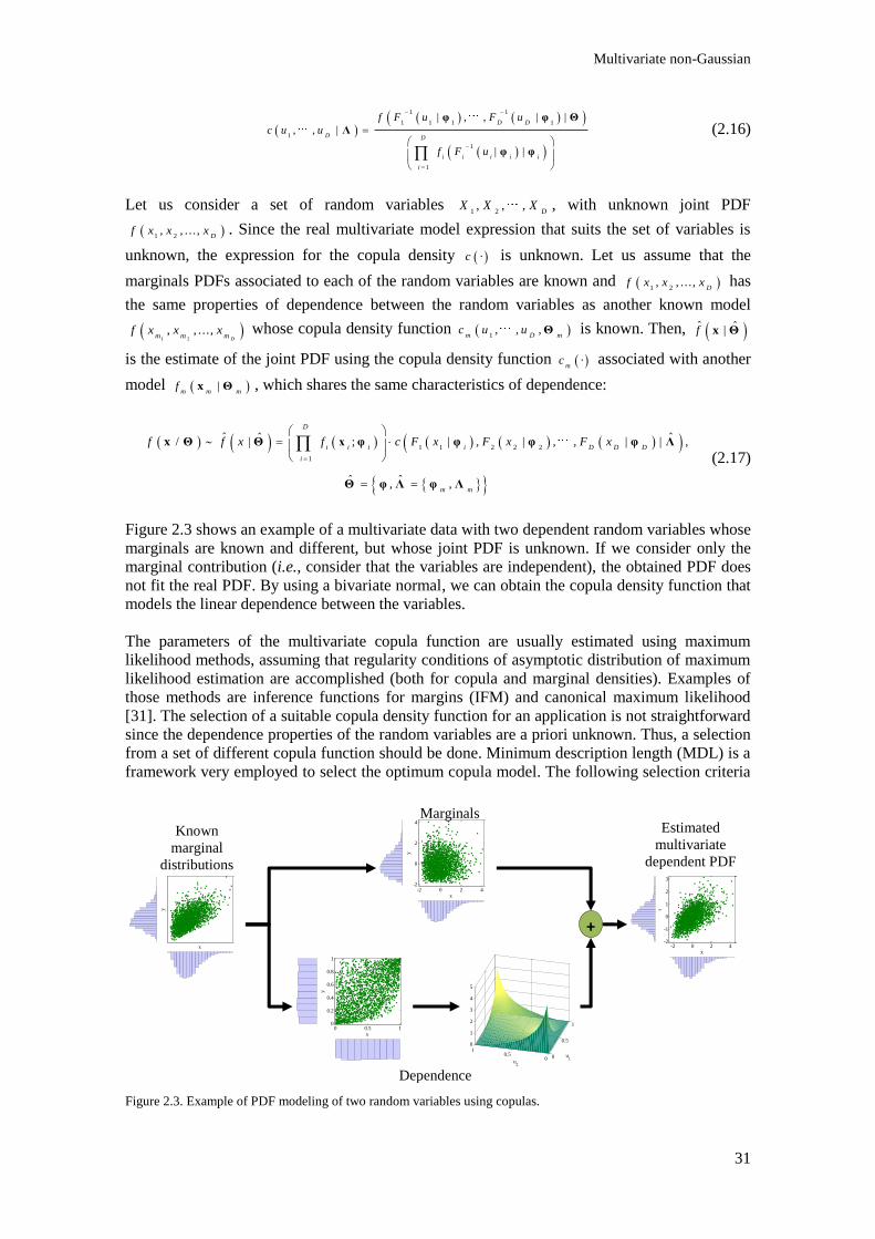
Multivariate non-Gaussian
31
1 1
1 1 1 1
1
1
1
| , , | |
, , |
| |
D D
D D
i i i i i
i
f F u F u
c u u
f F u
φ φ Θ
Λ
φ φ
(2.16)
Let us consider a set of random variables 1 2, , ,
DX X X , with unknown joint PDF
1 2, , . . . ,
Df x x x . Since the real multivariate model expression that suits the set of variables is
unknown, the expression for the copula density ·c is unknown. Let us assume that the
marginals PDFs associated to each of the random variables are known and 1 2, , . . . ,
Df x x x has
the same properties of dependence between the random variables as another known model
1 2
, , ...,D
m m mf x x x whose copula density function 1
, , ,m D m
c u u Θ is known. Then, ˆ ˆ|f x Θ
is the estimate of the joint PDF using the copula density function ·mc associated with another
model |m m m
f x Θ , which shares the same characteristics of dependence:
1 1 2 2 2
1
ˆ ˆ ˆ/ | ; | , | , , | | ,
ˆ ˆ, ,
D
i i i i D D D
i
m m
f f x f c F x F x F x
x Θ Θ x φ φ φ φ Λ
Θ φ Λ φ Λ
(2.17)
Figure 2.3 shows an example of a multivariate data with two dependent random variables whose
marginals are known and different, but whose joint PDF is unknown. If we consider only the
marginal contribution (i.e., consider that the variables are independent), the obtained PDF does
not fit the real PDF. By using a bivariate normal, we can obtain the copula density function that
models the linear dependence between the variables.
The parameters of the multivariate copula function are usually estimated using maximum
likelihood methods, assuming that regularity conditions of asymptotic distribution of maximum
likelihood estimation are accomplished (both for copula and marginal densities). Examples of
those methods are inference functions for margins (IFM) and canonical maximum likelihood
[31]. The selection of a suitable copula density function for an application is not straightforward
since the dependence properties of the random variables are a priori unknown. Thus, a selection
from a set of different copula function should be done. Minimum description length (MDL) is a
framework very employed to select the optimum copula model. The following selection criteria
Figure 2.3. Example of PDF modeling of two random variables using copulas.
0
0.5
1
00.5
10
1
2
3
4
5
u1
u2
x
y
-2 0 2 4-2
0
2
4
x
y
-2 0 2 4-2
-1
0
1
2
3
x
y
Known
marginal
distributions
0 0.5 10
0.2
0.4
0.6
0.8
1
x
y
Estimated
multivariate
dependent PDF
Marginals
Dependence
+
Chapter 2- Finite mixture models with non-Gaussian components
32
can be applied in MDL: Akaike information criterion (AIC), Bayesian information criterion
(BIC), stochastic information complexity (SIC), and normalized maximum likelihood (NML).
These criteria try to calculate a relative index that takes into account the tradeoff between model
performance and increase of complexity.
The copula function itself can be derived from known PDFs such as multivariate Gaussian,
multivariate t -Student, and mixtures of Gaussians. These copulas are called elliptic because the
contour curves of the random variables form ellipses representing symmetric dependence
relations [260]. Another family of copula functions are the so-called “Archimedean” that allow
the dependency in high variable dimension to be modeled using only one parameter. Examples
of this family are Clayton, Frank, and Gumbel copulas [172]. All of these methods model
specific dependency structures, expect GMM, which is able to model many structures of
arbitrary dependency. A more general method consists of using a hierarchical procedure where
the dependency is calculated for every pair of variables forming a copula tree that decomposes
the multivariate PDF [18].
2.3.2. Latent variable modeling
Latent variable modeling (LVM) assumes that in each group of the data the underlying discrete
distribution depends of some covariates that can be modeled through a set of latent variables.
These variables are random variables whose measured values are hidden. The properties of
these unrecorded variables can be extracted from the observed variables by means of a statistical
LVM that relates both kinds of variables. LVM has been increasingly studied and currently is a
booming field of research both in theoretical developments and in applications. Examples of
LVM in recent literature, to quote a few, include the following: covariate measurement error in
nonlinear models [42]; spatial statistics [208]; learning harmonium models with infinite latent
features using graphical undirected LVM [52]; tensor decomposition for LVM [11]; semi-
parametric and parametric LVM in the presence of measurable outcomes of mixed type
(continuous and ordinal) in medicine [248]; error and bias estimation in sources and
components using Monte Carlo estimators [271]; selection of latent variables for multiple
mixed-outcome models [289]; hierarchical Bayesian models using LVM for network data [194];
fast algorithms for computing deviance information criterion (DIC) of high-dimensional LVM
[46]; and extending the factor analysis from individual to groups of variables [137].
In this section, the main foundations of LVM are reviewed, but comprehensive literature can be
found in [27,246,243,28] and the references within. In general, LVM can be defined as a
generalized regression function that can be written as f E gX S , where f is a link
function, E is the expectation operator, X denotes a matrix of observed variables, S is a latent
structure, and g is some function that relates the latent structure to the observed variables. If,
upon a suitable choice of f , the function g is linear, then the resulting family of models is
covered by generalized linear regression theory [181].
When unrecorded variables are believed to influence only one recorded variable directly, they
are commonly modeled as noise. However, when they influence two or more measured
variables directly, the objective is to identify them and their influences, i.e., the causal relations
of (often unknown) unrecorded variables that influence multiple recorded variables. Frequently,
it is assumed that recorded variables do not influence unrecorded variables, although in some
cases recorded variables may influence one another. This is specified as conditional
independence of the observed variables given the latent variables, and thus
1
| |
N
j j ij j
i
p p x
x s s , where N is the total number of observed variables and j represents
a unit of analysis of a latent variable. This is also called “local independence.”

Multivariate non-Gaussian
33
The association between LVM and FMM can be defined by relating the data (observations) with
the variables of the generative probabilistic data model (latent structure). Let us consider the
following generative probabilistic process for GMM: (i) draw mixture proportions
~ D ir ic h le t ; (ii) for each mixture component k , draw 2
0~ 0,
kN ; (iii) for each data
point n , draw mixture assignment | ~n
z D isc re te and draw data point
| , ~ ,1n
n n zx z N . Given a dataset, the posterior distribution can be considered to reverse this
process and to estimate the distribution of the hidden structure that probably generated them.
The model can be represented with the factored joint distribution of its hidden and observed
variables. For GMM, this joint distribution is
2 2
0 0
1 1
, , , | , | | | | ,
K N
k i i i
k i
p z x p p p z p x z
(2.18)
where |p is the Dirichlet density, 2
0|p is the Gaussian density, |
ii z
p z is a
discrete distribution, and | ,i i
p x z is a Gaussian density centred at the i
z -th mean. Note that
local variables have terms inside the product over N data points, whereas global variables have
terms outside of this product. Thus, the posterior of the GMM can be estimated from its joint
distribution as
2
02
0 2
0
, , , | ,
, , , | ,
| ,
p z x
p z x
p x
(2.19)
This posterior can be used to examine the particular hidden structure that is manifest in the
observed data.
On the other hand, LVM can be represented as a probabilistic graphical model (PGM) where the
dependencies between the variables of the observed and latent variables are encoded. The
graphical model shows the structure of the factorized joint distribution and the flow of the
generative process. In this graph, nodes represent random variables and edges denote
dependence between them (Figure 2.4 shows an example of probabilistic graphical model for a
mixture of two Gaussians). PGM is related with signal processing on graphs, which is a field of
increasing research interest in applications of big data [66,67].
There are several kinds of LVMs, which are often categorized in terms of the type of observed
and latent variables, (i.e., continuous or categorical variables). Table 2.1 shows a classification
of classical LVMs.
Latent variables
Continuous Categorical
Observed
variables
Continuous Common factor model
Structural equation model
Linear mixed model
Covariate measurement error model
Latent profile model
Categorical Latent trail model (item-response
theory (IRT) model)
Latent class model
Table 2.1. Types of latent variable models.
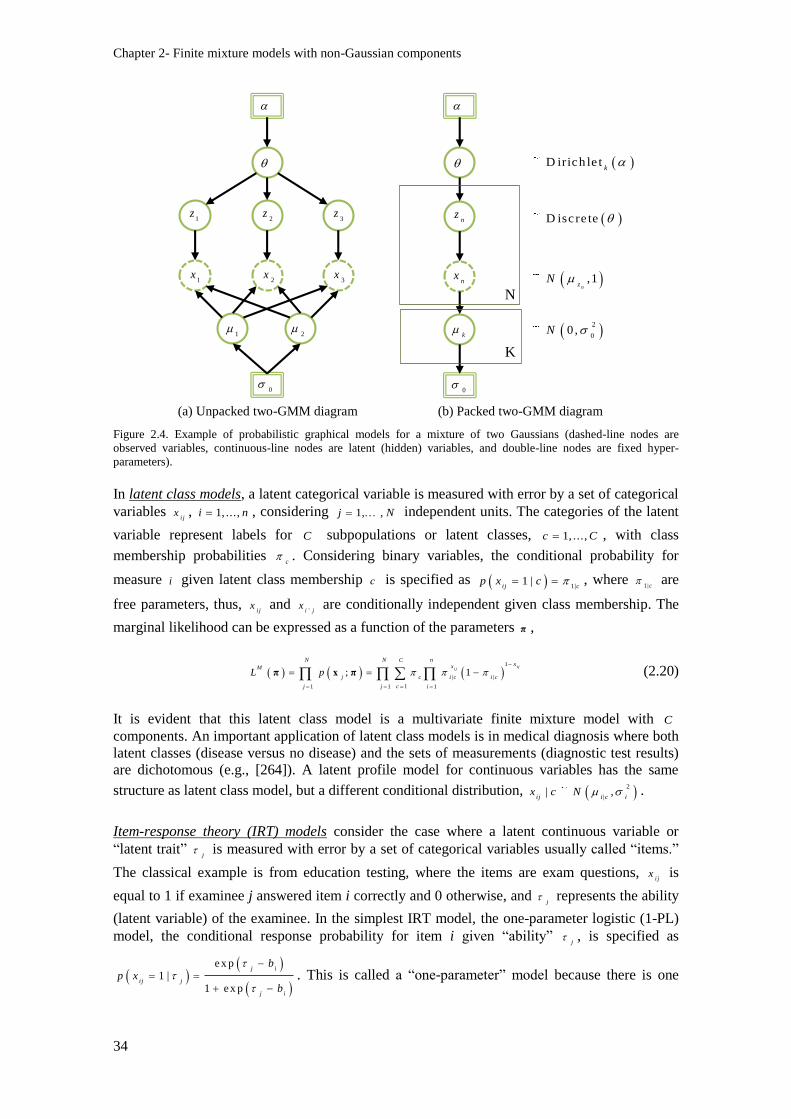
Chapter 2- Finite mixture models with non-Gaussian components
34
(a) Unpacked two-GMM diagram (b) Packed two-GMM diagram
Figure 2.4. Example of probabilistic graphical models for a mixture of two Gaussians (dashed-line nodes are
observed variables, continuous-line nodes are latent (hidden) variables, and double-line nodes are fixed hyper-
parameters).
In latent class models, a latent categorical variable is measured with error by a set of categorical
variables i j
x , 1, ...,i n , considering 1, ,j N independent units. The categories of the latent
variable represent labels for C subpopulations or latent classes, 1, ...,c C , with class
membership probabilities c
. Considering binary variables, the conditional probability for
measure i given latent class membership c is specified as 1|1 |
ij cp x c , where
1|c are
free parameters, thus, i j
x and 'i j
x are conditionally independent given class membership. The
marginal likelihood can be expressed as a function of the parameters π ,
1
| |
11 1 1
; 1ij
ij
N N nCxxM
j c i c i c
cj j i
L p
π x π (2.20)
It is evident that this latent class model is a multivariate finite mixture model with C
components. An important application of latent class models is in medical diagnosis where both
latent classes (disease versus no disease) and the sets of measurements (diagnostic test results)
are dichotomous (e.g., [264]). A latent profile model for continuous variables has the same
structure as latent class model, but a different conditional distribution, 2
|| ,
ij i c ix c N .
Item-response theory (IRT) models consider the case where a latent continuous variable or
“latent trait” j
is measured with error by a set of categorical variables usually called “items.”
The classical example is from education testing, where the items are exam questions, i j
x is
equal to 1 if examinee j answered item i correctly and 0 otherwise, and j
represents the ability
(latent variable) of the examinee. In the simplest IRT model, the one-parameter logistic (1-PL)
model, the conditional response probability for item i given “ability” j
, is specified as
e x p1 |
1 e x p
j i
i j j
j i
bp x
b
. This is called a “one-parameter” model because there is one
1z
2z
3z
1x
2x
3x
1
2
0
0
k
nz
nx
D irich le tk
D isc re te
,1n
zN
2
00 ,N
N
K
Multivariate non-Gaussian
35
parameter, “item difficulty” i
b , for each item. Assuming Gaussianity in distribution of the
random variable ability, a marginal likelihood can be easily estimated.
1-PL can be extended to a more general model that is more realistic. Thus, a two-parameter
logistic (2-PL) model can be specified, incorporating the 1-PL as a special case:
ex p
1 |
1 ex p
i j i
ij j
i j i
a b
p x
a b
. There are two parameters for each item, a discrimination
parameter i
a and an item difficulty parameter i
b . More complex IRT models accommodate
more parameters: guessing, rating scale, grade response, and so on. IRT models are extensively
applied in fields such as in sociology, social psychology, neuropsychology, and epidemiology
[261]. Some uncertainty arises from the kinds of variables involved in those applications since
they cannot be considered as strictly observable or at least measurable. The distinction between
observed and latent variables is of suggested epistemological character, i.e., accessible or not
epistemically accessible. For instance, intelligence quotient (IQ) scores are recorded, but general
intelligence is not; hence general intelligence is a latent variable and IQ and observed variable.
In addition, dealing with categorical variables is not easy and some bias is introduced by
assigning ranges of numerical values to the categories as observations of those variables [28].
In common factor analsys (CFA), it is assumed that each manifest variable is a function of f
common factors (i.e., latent variables that influence more than one manifest variable) and one
unique factor (i.e., a latent variable that influences only one manifest variable). This can be
described as [70]
T
F X Y L Z e (2.21)
where X is an [N × p] matrix of standardize scores on p manifest variables, Y is an [N × f]
matrix of standardized common factor scores; F
L is a [p × f] matrix of least square multiple
regression weights (the common factor pattern) for predicting the scores of X from those in Y ;
and Z is a [N × p] matrix of unique factors. The common and unique factors are uncorrelated
0T
Y Z and the unique factors for different manifest variables are uncorrelated as well, i.e,
2
T
N
Z ZU is a [p × p] diagonal matrix of unique factor variances. Because the unique factors
are uncorrelated with each other and with the common factors, it is possible to interpret Y as
containing common factors that account for correlations between manifest variables. Let us
assume an orthogonal common factor model, meaning that the f factors in Y are uncorrelated
with each other. Because of sampling error and model error (e.g., nonlinear relationships
between manifest variables and common factors, or minor factors), the common factor model
will almost never hold exactly, and therefore e ([N × p]) is included as a residual matrix. Thus,
(2.21) may be written as 2
T
T
F F
N
X XS L L U E , where S is a [p × p] sample correlation
matrix and E is a [p × p] matrix of residual correlations. Factor analysis procedures attempt to
keep E as small as possible by optimally choosing F
L and 2U . Estimation in CFA typically
employs an iterative procedure, where F
L is calculated at each 2U found by the algorithm. The
iterative principal axis factoring procedure is a popular method that provides a result which is
asymptotically equivalent to the unweighted least square discrepancy function. The squared
multiple correlations can be used as initial communalities. Factor scores are then calculated by
decomposing the reduced correlation matrix as
2T S V K V U (2.22)
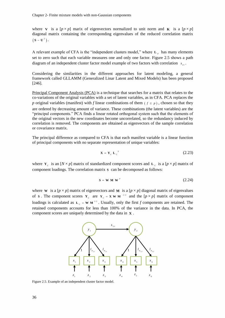
Chapter 2- Finite mixture models with non-Gaussian components
36
where V is a [p × p] marix of eigenvectors normalized to unit norm and K is a [p × p]
diagonal matrix containing the corresponding eigenvalues of the reduced correlation matrix
2
S U .
A relevant example of CFA is the “independent clusters model,” where F
L has many elements
set to zero such that each variable measures one and only one factor. Figure 2.5 shows a path
diagram of an independent cluster factor model example of two factors with correlation 2 1
s .
Considering the similarities in the different approaches for latent modeling, a general
framework called GLLAMM (Generalized Linar Latent and Mixed Models) has been proposed
[246].
Principal Component Analysis (PCA) is a technique that searches for a matrix that relates to the
co-variations of the original variables with a set of latent variables, as in CFA. PCA replaces the
p original variables (manifest) with f linear combinations of them f p , chosen so that they
are ordered by decreasing amount of variance. These combinations (the latent variables) are the
“principal components.” PCA finds a linear rotated orthogonal system such that the elements of
the original vectors in the new coordinates become uncorrelated, so the redundancy induced by
correlation is removed. The components are obtained as eigenvectors of the sample correlation
or covariance matrix.
The principal difference as compared to CFA is that each manifest variable is a linear function
of principal components with no separate representation of unique variables:
T
C CX Y L (2.23)
where C
Y is an [N × p] matrix of standardized component scores and C
L is a [p × p] matrix of
component loadings. The correlation matrix S can be decomposed as follows:
TS W M W (2.24)
where W is a [p × p] matrix of eigenvectors and M is a [p × p] diagonal matrix of eigenvalues
of S . The component scores C
Y are 1 / 2
C
Y X W M and the [p × p] matrix of component
loadings is calculated as 1 / 2
CL W M . Usually, only the first f components are retained. The
retained components accounts for less than 100% of the variance in the data. In PCA, the
component scores are uniquely determined by the data in X .
Figure 2.5. Example of an independent cluster factor model.
1y
2y
1x
2x
3x
4x
5x
6x
1z
2z
3z
4z 5
z6
z
2 1F
l3 1
Fl
5 2F
l6 2
Fl1 1
2 1s
Multivariate non-Gaussian
37
From equations (2.22) and (2.24), we can conclude that the main difference between CFA and
PCA is that CFA involves a reduction of the diagonal elements of the correlation matrix
whereas PCA does not. CFA explains the off-diagonal elements of S according to a
discrepancy function. In contrast, the retained components in PCA optimally account for the 1s
of the diagonal of S ; i.e., for r retained components, r r
T
C CL L maximizes t r S among all
possible orthogonal linear transformations of X . Thus, the principal objective of PCA is to
optimally estimate the maximum amount of variance with the minimum number of components.
In addition, it can be demonstrated that the difference between CFA and PCA loadings will be
small when the unique variances in 2U are small.
The analysis of the differences between PCA and CFA has covered aspects such as factors and
component loadings depending on the number of variables (similarity increases as the number
of variables increases since the diagonal elements increase arithmetically but the off-diagonal
elements increase geometrically); data sphericity condition; and generalizability of results, i.e.,
consistency of factors and components for different subsets of variables (see for instance
[70,263,187]).
A natural evolution of statistical signal processing, in connection with the progressive increase
in computational power, has been the extension of PCA (based on second order statistics and
correlation) to ICA (based on independence) for exploiting higher-order information. In the next
section, we approach ICA, which is a multivariate statistical method that is particularly suitable
for uncovering latent source signals from high-dimensional complex data.
2.3.3. Independent component analysis (ICA)
Independent component analysis was introduced by C. Jutten in [132,129,130,131], although its
first thorough mathematical formulation was performed by P. Comon [60]. Since then, many
different algorithms have been proposed for estimating the ICA parameters (see for example
[111,55,150,56,59]). The large number of applied problems where ICA has been considered as a
practical solution is also remarkable.
ICA is formulated as a linear model of the observed data vector 1, ...,
T
Mx n x n x = which is
assumed to be a linear transformation of a vector 1, ...,
T
Ms n s n s = in the form (we assume
for simplicity the square model, where A is a square [M × M] matrix):
x = A s (2.25)
The elements of s are assumed to be statistically independent components [111], while
dependence is allowed among the elements of x: every component of x is generated from a
linear combination of the same independent variables 1, ...,
Ms s . This simple model can be seen
from different perspectives. The most obvious is that of modeling multivariate probability
density functions in presence of statistical dependence. If A is square and invertible, we may
express the joint probability density xp x in terms of 1
. . .·s M
p p s p s s in the form
11
d e tX S
p p
x = A xA
(2.26)
Thus, the joint probability modeling is decomposed into two parts: modeling of the marginal
densities 1. . .·
Mp s p s (which implies M univariate models) and estimating the mixing
matrix A, which is the responsible for the statistical dependence among the elements of x. As
long as the marginal are non-Gaussian, xp x will be multivariate non-Gaussian. Notice the
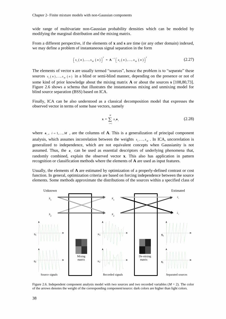
Chapter 2- Finite mixture models with non-Gaussian components
38
wide range of multivariate non-Gaussian probability densities which can be modeled by
modifying the marginal distribution and the mixing matrix.
From a different perspective, if the elements of x and s are time (or any other domain) indexed,
we may define a problem of instantaneous signal separation in the form
1
1 1, ..., , ...,
T T
M Ms n s n x n x n
= A (2.27)
The elements of vector s are usually termed “sources”, hence the problem is to “separate” these
sources 1, . . . ,
Ms n s n in a blind or semi-blind manner, depending on the presence or not of
some kind of prior knowledge about the mixing matrix A or about the sources s [108,80,73].
Figure 2.6 shows a schema that illustrates the instantaneous mixing and unmixing model for
blind source separation (BSS) based on ICA.
Finally, ICA can be also understood as a classical decomposition model that expresses the
observed vector in terms of some base vectors, namely
1
M
i i
i
s=
x = a (2.28)
where i
a , 1, ...,i M , are the columns of A. This is a generalization of principal component
analysis, which assumes incorrelation between the weights 1, ...,
Ms s . In ICA, uncorrelation is
generalized to independence, which are not equivalent concepts when Gaussianity is not
assumed. Thus, the i
a can be used as essential descriptors of underlying phenomena that,
randomly combined, explain the observed vector x. This also has application in pattern
recognition or classification methods where the elements of A are used as input features.
Usually, the elements of A are estimated by optimization of a properly-defined contrast or cost
function. In general, optimization criteria are based on forcing independence between the source
elements. Some methods approximate the distributions of the sources within a specified class of
Figure 2.6. Independent component analysis model with two sources and two recorded variables (M = 2). The color
of the arrows denotes the weight of the corresponding component/source: dark colors are higher than light colors.
Unknown Estimated
s1
s2
x1
x2
1s
2s
s1
s2
Source signals
Mixing
matrix
x1
x2
Recorded signals
De-mixing
matrix
s1
s2
Separated sources
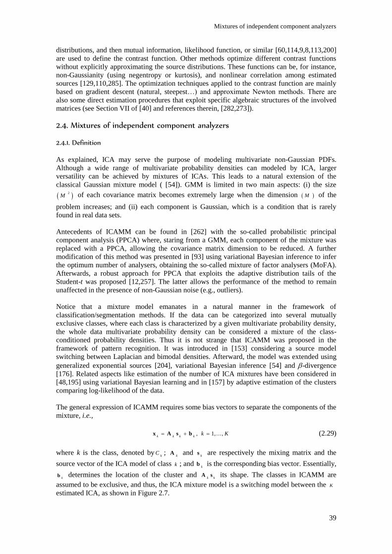
Mixtures of independent component analyzers
39
distributions, and then mutual information, likelihood function, or similar [60,114,9,8,113,200]
are used to define the contrast function. Other methods optimize different contrast functions
without explicitly approximating the source distributions. These functions can be, for instance,
non-Gaussianity (using negentropy or kurtosis), and nonlinear correlation among estimated
sources [129,110,285]. The optimization techniques applied to the contrast function are mainly
based on gradient descent (natural, steepest…) and approximate Newton methods. There are
also some direct estimation procedures that exploit specific algebraic structures of the involved
matrices (see Section VII of [40] and references therein, [282,273]).
2.4. Mixtures of independent component analyzers 2.4.1. Definition
As explained, ICA may serve the purpose of modeling multivariate non-Gaussian PDFs.
Although a wide range of multivariate probability densities can modeled by ICA, larger
versatility can be achieved by mixtures of ICAs. This leads to a natural extension of the
classical Gaussian mixture model ( [54]). GMM is limited in two main aspects: (i) the size
2
M of each covariance matrix becomes extremely large when the dimension M of the
problem increases; and (ii) each component is Gaussian, which is a condition that is rarely
found in real data sets.
Antecedents of ICAMM can be found in [262] with the so-called probabilistic principal
component analysis (PPCA) where, staring from a GMM, each component of the mixture was
replaced with a PPCA, allowing the covariance matrix dimension to be reduced. A further
modification of this method was presented in [93] using variational Bayesian inference to infer
the optimum number of analysers, obtaining the so-called mixture of factor analysers (MoFA).
Afterwards, a robust approach for PPCA that exploits the adaptive distribution tails of the
Student-t was proposed [12,257]. The latter allows the performance of the method to remain
unaffected in the presence of non-Gaussian noise (e.g., outliers).
Notice that a mixture model emanates in a natural manner in the framework of
classification/segmentation methods. If the data can be categorized into several mutually
exclusive classes, where each class is characterized by a given multivariate probability density,
the whole data multivariate probability density can be considered a mixture of the class-
conditioned probability densities. Thus it is not strange that ICAMM was proposed in the
framework of pattern recognition. It was introduced in [153] considering a source model
switching between Laplacian and bimodal densities. Afterward, the model was extended using
generalized exponential sources [204], variational Bayesian inference [54] and -divergence
[176]. Related aspects like estimation of the number of ICA mixtures have been considered in
[48,195] using variational Bayesian learning and in [157] by adaptive estimation of the clusters
comparing log-likelihood of the data.
The general expression of ICAMM requires some bias vectors to separate the components of the
mixture, i.e.,
, 1, ...,k k k k
k K x A s b (2.29)
where k is the class, denoted byk
C ; k
A and k
s are respectively the mixing matrix and the
source vector of the ICA model of class k ; and k
b is the corresponding bias vector. Essentially,
kb determines the location of the cluster and
k kA s its shape. The classes in ICAMM are
assumed to be exclusive, and thus, the ICA mixture model is a switching model between the K
estimated ICA, as shown in Figure 2.7.
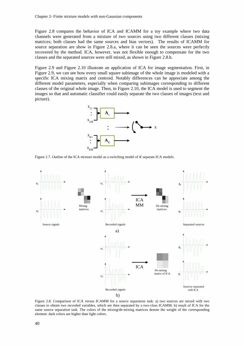
Chapter 2- Finite mixture models with non-Gaussian components
40
Figure 2.8 compares the behavior of ICA and ICAMM for a toy example where two data
channels were generated from a mixture of two sources using two different classes (mixing
matrices; both classes had the same sources and bias vectors). The results of ICAMM for
source separation are show in Figure 2.8.a, where it can be seen the sources were perfectly
recovered by the method. ICA, however, was not flexible enough to compensate for the two
classes and the separated sources were still mixed, as shown in Figure 2.8.b.
Figure 2.9 and Figure 2.10 illustrate an application of ICA for image segmentation. First, in
Figure 2.9, we can see how every small square subimage of the whole image is modeled with a
specific ICA mixing matrix and centroid. Notably differences can be appreciate among the
different model parameters, especially when comparing subimages corresponding to different
classes of the original whole image. Then, in Figure 2.10, the ICA model is used to segment the
images so that and automatic classifier could easily separate the two classes of images (text and
picture).
Figure 2.7. Outline of the ICA mixture model as a switching model of K separate ICA models.
Figure 2.8. Comparison of ICA versus ICAMM for a source separation task: a) two sources are mixed with two
classes to obtain two recorded variables, which are then separated by a two-class ICAMM; b) result of ICA for the
same source separation task. The colors of the mixing/de-mixing matrices denote the weight of the corresponding
element: dark colors are higher than light colors.
A1
AK
s11
s1M
sK1
sKM
…
…
…
x
s1
s2
Source signals
Mixing
matrices
x1
x2
Recorded signals
De-mixing
matrices
s1
s2
Separated sources
De-mixing
matrix of ICA
s1
s2
Sources separated
with ICA
ICA
MM
ICA
a)
b)
s1
s2
Source signals
Mixing
matrices
x1
x2
Recorded signals
De-mixing
matrices
s1
s2
Separated sources
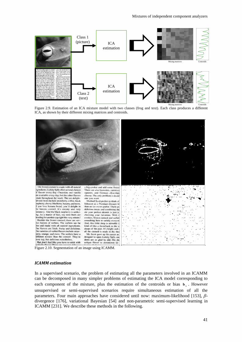
Mixtures of independent component analyzers
41
Figure 2.9. Estimation of an ICA mixture model with two classes (frog and text). Each class produces a different
ICA, as shown by their different mixing matrices and centroids.
Figure 2.10. Segmentation of an image using ICAMM.
ICAMM estimation
In a supervised scenario, the problem of estimating all the parameters involved in an ICAMM
can be decomposed in many simpler problems of estimating the ICA model corresponding to
each component of the mixture, plus the estimation of the centroids or bias k
b . However
unsupervised or semi-supervised scenarios require simultaneous estimation of all the
parameters. Four main approaches have considered until now: maximum-likelihood [153], -
divergence [176], variational Bayesian [54] and non-parametric semi-supervised learning in
ICAMM [231]. We describe these methods in the following.
Class 1 (picture)
Class 2 (text)
ICA
estimation
ICA
estimation
Mixing matrices Centroids
Mixing matrices Centroids
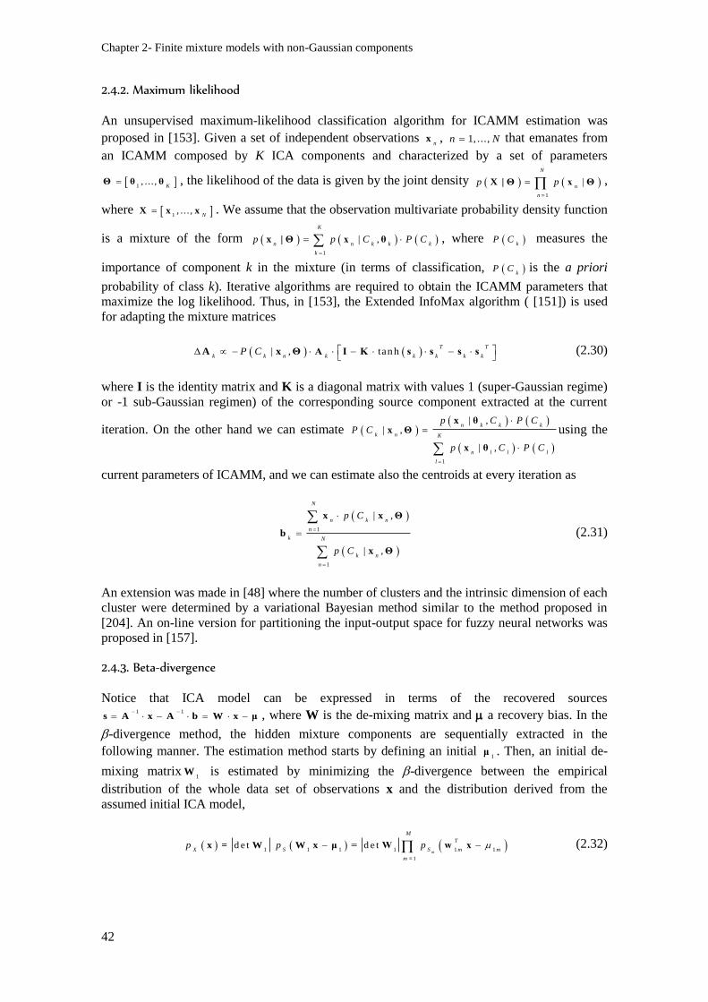
Chapter 2- Finite mixture models with non-Gaussian components
42
2.4.2. Maximum likelihood
An unsupervised maximum-likelihood classification algorithm for ICAMM estimation was
proposed in [153]. Given a set of independent observations n
x , 1, ...,n N that emanates from
an ICAMM composed by K ICA components and characterized by a set of parameters
1, . . . ,
KΘ θ θ , the likelihood of the data is given by the joint density
1
|
N
n
n
p p
X | Θ x Θ ,
where 1, . . . ,
NX x x . We assume that the observation multivariate probability density function
is a mixture of the form 1
| ,
K
n n k k k
k
p p C P C
x | Θ x θ , where kP C measures the
importance of component k in the mixture (in terms of classification, kP C is the a priori
probability of class k). Iterative algorithms are required to obtain the ICAMM parameters that
maximize the log likelihood. Thus, in [153], the Extended InfoMax algorithm ( [151]) is used
for adapting the mixture matrices
| , tanhT T
k k n k k k k kP C
A x Θ A I K s s s s (2.30)
where I is the identity matrix and K is a diagonal matrix with values 1 (super-Gaussian regime)
or -1 sub-Gaussian regimen) of the corresponding source component extracted at the current
iteration. On the other hand we can estimate
1
| ,| ,
| ,
n k k k
k n K
n l l l
l
p C P CP C
p C P C
x θx Θ
x θ
using the
current parameters of ICAMM, and we can estimate also the centroids at every iteration as
1
1
| ,
| ,
N
n k n
n
k N
k n
n
p C
p C
x x Θ
b
x Θ
(2.31)
An extension was made in [48] where the number of clusters and the intrinsic dimension of each
cluster were determined by a variational Bayesian method similar to the method proposed in
[204]. An on-line version for partitioning the input-output space for fuzzy neural networks was
proposed in [157].
2.4.3. Beta-divergence
Notice that ICA model can be expressed in terms of the recovered sources 1 1
s A x A b W x μ , where W is the de-mixing matrix and a recovery bias. In the
-divergence method, the hidden mixture components are sequentially extracted in the
following manner. The estimation method starts by defining an initial 1
μ . Then, an initial de-
mixing matrix1
W is estimated by minimizing the -divergence between the empirical
distribution of the whole data set of observations x and the distribution derived from the
assumed initial ICA model,
1 1 1 1 1 1
1
d e t d e tm
M
T
X S S m m
m
p p p =
x = W W x μ = W w x (2.32)
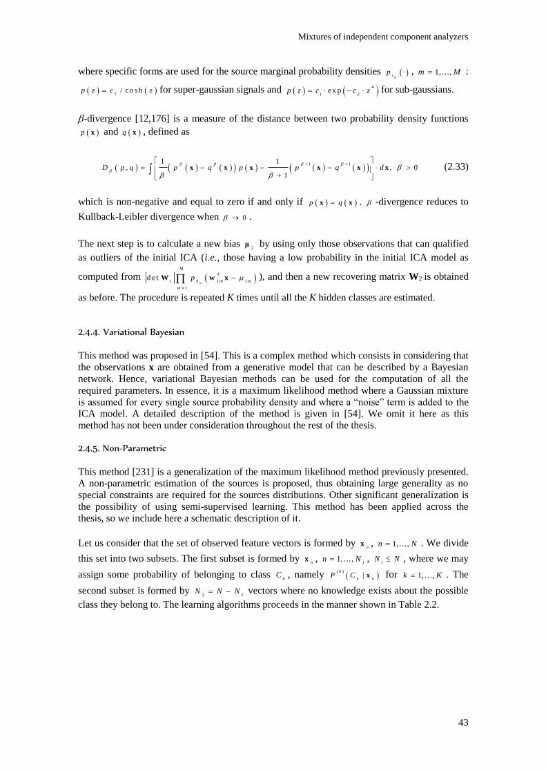
Mixtures of independent component analyzers
43
where specific forms are used for the source marginal probability densities ·m
sp , 1, ...,m M :
2/ c o s hp z c z for super-gaussian signals and
4
1 2ex pp z c c z for sub-gaussians.
-divergence [12,176] is a measure of the distance between two probability density functions
p x and q x , defined as
1 11 1
, , 01
D p q p q p p q d
x x x x x x (2.33)
which is non-negative and equal to zero if and only if p qx x . -divergence reduces to
Kullback-Leibler divergence when 0 .
The next step is to calculate a new bias 2
μ by using only those observations that can qualified
as outliers of the initial ICA (i.e., those having a low probability in the initial ICA model as
computed from 1 1 1
1
d e tm
M
T
S m m
m
p =
W w x ), and then a new recovering matrix W2 is obtained
as before. The procedure is repeated K times until all the K hidden classes are estimated.
2.4.4. Variational Bayesian
This method was proposed in [54]. This is a complex method which consists in considering that
the observations x are obtained from a generative model that can be described by a Bayesian
network. Hence, variational Bayesian methods can be used for the computation of all the
required parameters. In essence, it is a maximum likelihood method where a Gaussian mixture
is assumed for every single source probability density and where a “noise” term is added to the
ICA model. A detailed description of the method is given in [54]. We omit it here as this
method has not been under consideration throughout the rest of the thesis.
2.4.5. Non-Parametric
This method [231] is a generalization of the maximum likelihood method previously presented.
A non-parametric estimation of the sources is proposed, thus obtaining large generality as no
special constraints are required for the sources distributions. Other significant generalization is
the possibility of using semi-supervised learning. This method has been applied across the
thesis, so we include here a schematic description of it.
Let us consider that the set of observed feature vectors is formed by n
x , 1, ...,n N . We divide
this set into two subsets. The first subset is formed by n
x , 1
1, ...,n N , 1
N N , where we may
assign some probability of belonging to class k
C , namely
0
|k n
P C x for 1, ...,k K . The
second subset is formed by 2 1
N N N vectors where no knowledge exists about the possible
class they belong to. The learning algorithms proceeds in the manner shown in Table 2.2.
Chapter 2- Finite mixture models with non-Gaussian components
44
Initialization
For 1 ...k K , compute:
1
0 0
1
|
N
k n k n
n
P C
b x x (if 1
0M , select the initial centroids randomly);
0
kW (randomly initialized) ;
0 0 0
kn k n k s W x b
0 0 0
km k m k s W x b
0
kp s (a non-parametric estimator is used)
Updating
For 1 ... Ii and for 1 ...k K , compute:
For the probabilistically labeled vectors
0
1| | , 1, .. . ,
i
k n k nP C P C n N x x
For the unlabeled vectors,
1 1 1 1 1 1
' ' '
' 1
| |
d e t d e t
i i
k n n k k n
K
i i i i i i
k kn k k k m k
k
P C p C P C p
p P C p P C
x x x
W s W s
, 1
1, ...,n N N
1
|
N
i i
k n k n
n
P C
b x x ;
1 1i i i
k k k
W W W ,
1 1 1
1
|
N
i i i
k k nkn IC A
n
P C
W W x ; where
1i
kn IC A
W is the update due to sample n
x in the selected embedded ICA algorithm;
i i i
kn k n k s W x b
i i
k np s (a non-parametric estimate is used, e.g., by the kernel method).
Table 2.2. Non-parametric learning algorithm.
2.5. Conclusions
The main objective of this chapter has been to situate ICAMM in the context of non-Gaussian
mixture models of the underlying probability density of a set of observations. Non-Gaussian
mixtures are the natural extension of Gaussian mixtures. However, there is significantly less
literature on non-Gaussian mixtures than in Gaussian mixtures, due to the lack of general
methods for optimum estimation of the mixture parameters. Thus, non-Gaussian mixtures pose
attractive challenges for further work.
We have started by considering the univariate case. The techniques presented in this chapter
assume the same type of probability for all the mixture components, thus easing the problem of
estimating the corresponding parameters at the price of some loss of adaptation to specific
scenarios. Different non-Gaussian densities have been considered: Exponential, Poisson,
binomial and multinomial. They are illustrative of both continuous and discrete random
variables, although many other types of distributions could be devised.
The extension of univariate mixtures to the multivariate case is immediate if it can be assumed
that the components of the multivariate random variable are statistically independent, so that the
multivariate probability density can be expressed as the product of the marginals. Then, every
marginal can be modeled as a mixture of univariate densities. In presence of statistical
dependence, however, the extension is not so easy. Firstly, the extension of typical univariate
densities to their corresponding multivariate is not trivial or even possible in most cases. A

Conclusions
45
notable exception is the multivariate Gaussian case, where dependence is parameterized by a
covariance matrix. Hence we have considered in this chapter three methods for multivariate
modeling of a non-Gaussian and non-independent probability density: copulas, latent variables
and ICA. The latter may be considered a special case of the latent variables method. Regarding
the copulas, it is outside the scope of this thesis a detailed comparison with ICA. In fact,
mixtures of copulas have not been considered until now, while some methods exist for
computing mixtures of ICAs. We have presented four of these methods: maximum likelihood,
-divergence, variational Bayes and non-parametric. Due to its generality, the latter will be
mostly used across the thesis for estimating the ICAMM parameters in the two main problems
considered: prediction based on ICAMM and extension of ICAMM to dynamic non-stationary
scenarios.

47
Building non-linear prediction structures from independent component analysis
3

49
- Building non-linear prediction structures from independent component analysis
This chapter presents two novel non-linear prediction methods that are based on independent
component analysis mixture modeling. The first method is based on the maximization of the
log-likelihood of the data with respect to the ICAMM parameters. We have called this method
PREDICAMM (Prediction using ICAMM). The second method is an approximation of the
optimal predictor with respect to the mean squared error of the prediction: the conditional
expectation of missing data with respect to known data and the ICAMM parameters. This
second method we have named E-ICAMM (Expectation assuming ICAMM). Unlike pre-
existing methods, these algorithms do not use ICA mixture models as a pre-processing step, but
as the base of the prediction itself, since they use of both known data and the ICAMM to predict
missing data.
PREDICAMM performs the maximization of the log-likelihood of the data with a gradient.
Therefore, we performed a sensitivity analysis in order to determine the effect of the initial
value and the number of classes in the results of this prediction algorithm.
The performance of the proposed predictors was assessed by prediction missing values in
synthetic data modeled with two, three and four classes. In order to test the sensitivity of
PREDICAMM and E-ICAMM when the base assumptions are not completely fulfilled, the
performance was also tested on several sets of nonlinearly-corrupted data. In all cases, the
proposed predictor was compared with four other classical and state-of-the-art methods: matrix
completion (a non-linear method that makes use of the structure of a matrix); splines (a
commonly-used interpolation method); Wiener structures (a combination of a linear predictor
and a non-linear correction); and Kriging (a classical linear predictor that is commonly used in
geostatistical applications). The comparison shows that the proposed ICAMM-based methods
can be competitive for data prediction even if the basic conditions of ICAMM are not satisfied.
In addition, the proposed methods usually performed better than Wiener structures, matrix
completion, splines and Kriging. Finally, we performed a last experiment to test the
performance of the proposed methods with respect to an increasing number of missing values in
each observation. Some of the simulations in this chapter have been reported in [219,224], and
results for real-data applications are included in Chapter 5.
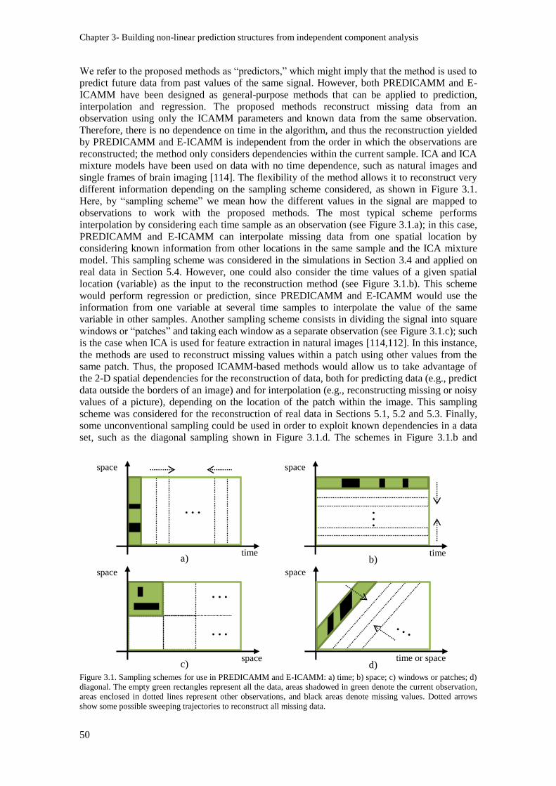
Chapter 3- Building non-linear prediction structures from independent component analysis
50
We refer to the proposed methods as “predictors,” which might imply that the method is used to
predict future data from past values of the same signal. However, both PREDICAMM and E-
ICAMM have been designed as general-purpose methods that can be applied to prediction,
interpolation and regression. The proposed methods reconstruct missing data from an
observation using only the ICAMM parameters and known data from the same observation.
Therefore, there is no dependence on time in the algorithm, and thus the reconstruction yielded
by PREDICAMM and E-ICAMM is independent from the order in which the observations are
reconstructed; the method only considers dependencies within the current sample. ICA and ICA
mixture models have been used on data with no time dependence, such as natural images and
single frames of brain imaging [114]. The flexibility of the method allows it to reconstruct very
different information depending on the sampling scheme considered, as shown in Figure 3.1.
Here, by “sampling scheme” we mean how the different values in the signal are mapped to
observations to work with the proposed methods. The most typical scheme performs
interpolation by considering each time sample as an observation (see Figure 3.1.a); in this case,
PREDICAMM and E-ICAMM can interpolate missing data from one spatial location by
considering known information from other locations in the same sample and the ICA mixture
model. This sampling scheme was considered in the simulations in Section 3.4 and applied on
real data in Section 5.4. However, one could also consider the time values of a given spatial
location (variable) as the input to the reconstruction method (see Figure 3.1.b). This scheme
would perform regression or prediction, since PREDICAMM and E-ICAMM would use the
information from one variable at several time samples to interpolate the value of the same
variable in other samples. Another sampling scheme consists in dividing the signal into square
windows or “patches” and taking each window as a separate observation (see Figure 3.1.c); such
is the case when ICA is used for feature extraction in natural images [114,112]. In this instance,
the methods are used to reconstruct missing values within a patch using other values from the
same patch. Thus, the proposed ICAMM-based methods would allow us to take advantage of
the 2-D spatial dependencies for the reconstruction of data, both for predicting data (e.g., predict
data outside the borders of an image) and for interpolation (e.g., reconstructing missing or noisy
values of a picture), depending on the location of the patch within the image. This sampling
scheme was considered for the reconstruction of real data in Sections 5.1, 5.2 and 5.3. Finally,
some unconventional sampling could be used in order to exploit known dependencies in a data
set, such as the diagonal sampling shown in Figure 3.1.d. The schemes in Figure 3.1.b and
Figure 3.1. Sampling schemes for use in PREDICAMM and E-ICAMM: a) time; b) space; c) windows or patches; d)
diagonal. The empty green rectangles represent all the data, areas shadowed in green denote the current observation,
areas enclosed in dotted lines represent other observations, and black areas denote missing values. Dotted arrows
show some possible sweeping trajectories to reconstruct all missing data.
d) time or space
space
a) time
space
…
c) space
space
…
…
11111
b) time
space
…
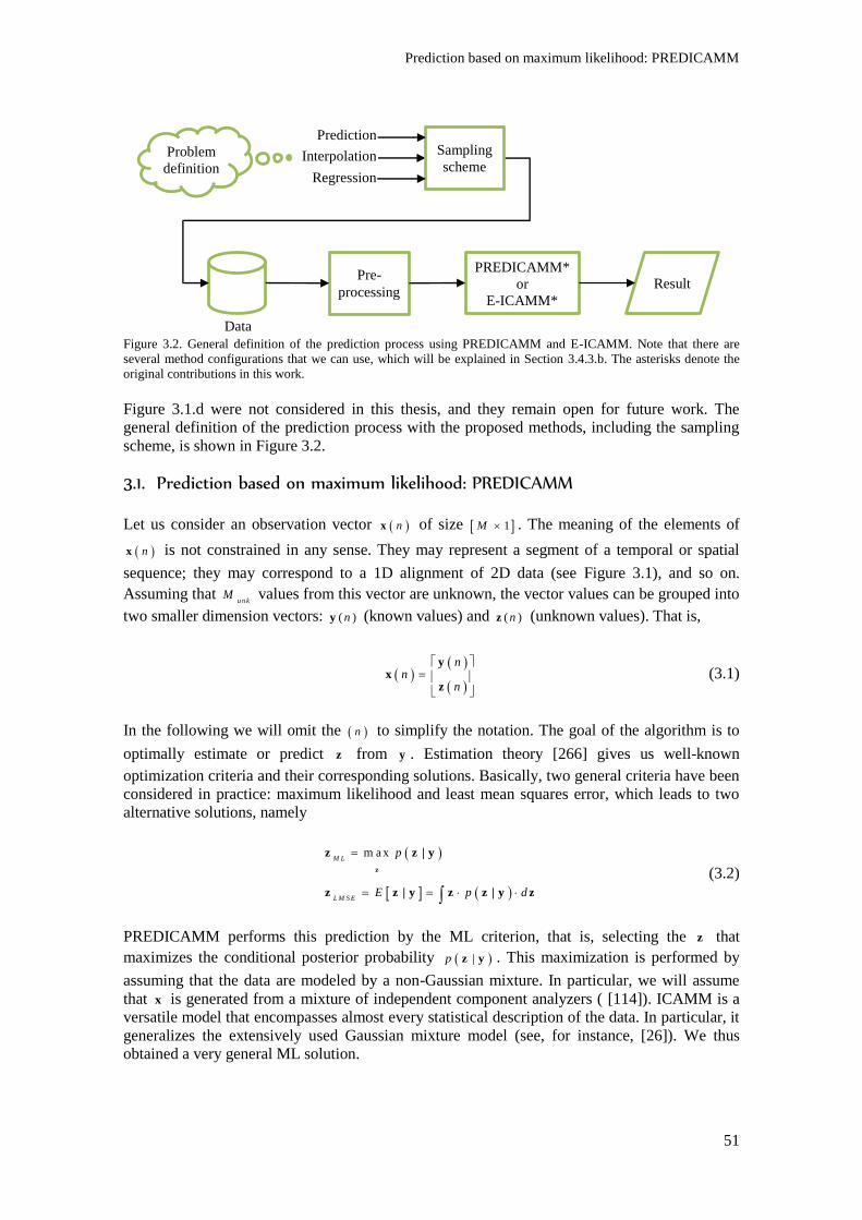
Prediction based on maximum likelihood: PREDICAMM
51
Figure 3.2. General definition of the prediction process using PREDICAMM and E-ICAMM. Note that there are
several method configurations that we can use, which will be explained in Section 3.4.3.b. The asterisks denote the
original contributions in this work.
Figure 3.1.d were not considered in this thesis, and they remain open for future work. The
general definition of the prediction process with the proposed methods, including the sampling
scheme, is shown in Figure 3.2.
3.1. Prediction based on maximum likelihood: PREDICAMM
Let us consider an observation vector nx of size 1M . The meaning of the elements of
nx is not constrained in any sense. They may represent a segment of a temporal or spatial
sequence; they may correspond to a 1D alignment of 2D data (see Figure 3.1), and so on.
Assuming that u n k
M values from this vector are unknown, the vector values can be grouped into
two smaller dimension vectors: ( )ny (known values) and ( )nz (unknown values). That is,
nn
n
yx
z (3.1)
In the following we will omit the n to simplify the notation. The goal of the algorithm is to
optimally estimate or predict z from y . Estimation theory [266] gives us well-known
optimization criteria and their corresponding solutions. Basically, two general criteria have been
considered in practice: maximum likelihood and least mean squares error, which leads to two
alternative solutions, namely
m a xM L
L M S E
p
E p d
z
z z | y
z z | y z z | y z
(3.2)
PREDICAMM performs this prediction by the ML criterion, that is, selecting the z that
maximizes the conditional posterior probability |p z y . This maximization is performed by
assuming that the data are modeled by a non-Gaussian mixture. In particular, we will assume
that x is generated from a mixture of independent component analyzers ( [114]). ICAMM is a
versatile model that encompasses almost every statistical description of the data. In particular, it
generalizes the extensively used Gaussian mixture model (see, for instance, [26]). We thus
obtained a very general ML solution.
Problem
definition
Data
Pre-
processing
PREDICAMM*
or
E-ICAMM* Result
Sampling
scheme
Prediction
Interpolation
Regression

Chapter 3- Building non-linear prediction structures from independent component analysis
52
Unfortunately, |p z y is complicated to calculate even if the underlying ICA mixture model is
known. Using Bayes’ rule, however, it can be seen that p p pz | y y , z y . The
maximization of p z | y is equivalent to the maximization of p y , z , since known data (and
thus p y ) are fixed during maximization. Given the ICA mixture model, the calculation of the
joint probability density p y , z (and its derivatives) is much easier than the calculation of the
conditional probability density, since p py , z x . Thus, we will seek the maximization of
p y , z in the following.
Let us assume that data x can be modeled using an ICA mixture model with K classes, where
the parameters of the model are known: the de-mixing matrices, k
W ; the probability density
function of the sources, kp s ; and the centroids,
kb ; where 1, ...,k K is the class. Then,
p x can be expressed as
1 1
| d e t
K K
k k k k k
k k
p p C P C p n P C
x x W s (3.3)
where the sources are calculated from the data using the ICAMM parameters, i.e.,
k k kn n s W x b ; and
kC denotes class k . It is possible to develop this equation a bit
further in order to separate the contribution to the sources of known data from the contribution
of unknown data. Each de-mixing matrix k
W can be treated as a block matrix such that
, ,k k k y z
W W W , where , ky
W is composed of the first u n k
M M columns of matrix k
W and
, kzW is composed of the last
u n kM columns of matrix
kW . Then, the sources can be calculated
as
, , , ,k k k k k k k k
y z y z
ys W W b W y W z W b
z (3.4)
, k
zW z is the only term in (3.4) that changes during the maximization process, since the
ICAMM parameters and the known data remain constant.
Equation (3.3) is maximized by using a gradient algorithm, with the joint probability density as
the cost function J z . We obtain the derivative of the cost function with respect to the
unknowns z :
1
,d e t
K
k
k k
k
J p pP C
z y z s
Wz z z
(3.5)
,
1 ,
M
k mk k
m k m
sp p
s
s s
z z (3.6)
where ,k m
s is the -thm component of the sources from the class k . The calculation of the
derivative of ( )k
p s in (3.6) is very complex for most data distributions, since it is the derivative
of a multi-dimensional probability density. However, each class from the ICAMM is modeled
by a separate ICA, so we can make use of the independence of the sources (a basic property of
the ICA model) to ease our calculations:
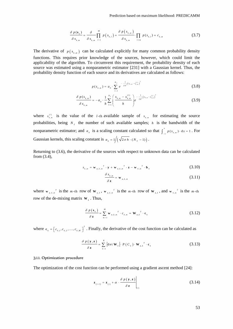
Prediction based on maximum likelihood: PREDICAMM
53
,
, , ,
1, , ,
( )( )
Mk mk
k l k l k m
l l mk m k m k m
p spp s p s c
s s s
s
(3.7)
The derivative of ,k mp s can be calculated explicitly for many common probability density
functions. This requires prior knowledge of the sources, however, which could limit the
applicability of the algorithm. To circumvent this requirement, the probability density of each
source was estimated using a nonparametric estimator [231] with a Gaussian kernel. Thus, the
probability density function of each source and its derivatives are calculated as follows:
2( )
, ,2
1
2
, 0
1
( )
l
k m k mT s s
h
m
l
k
N
p s a e
(3.8)
( )
, ,
2
2
1( )
, , , 2
0
1,
( ) 1l
k m kT
m
lN
k m k m k m h
lk m
s sp s s sa e
s h h
(3.9)
where ( )
,
l
k ms is the value of the -thl available sample of
,k ms for estimating the source
probabilities, being T
N the number of such available samples; h is the bandwidth of the
nonparametric estimator; and 0
a is a scaling constant calculated so that ,
( ) d 1k m
p s s
. For
Gaussian kernels, this scaling constant is 01 2 ( 1)
Ta h N .
Returning to (3.6), the derivative of the sources with respect to unknown data can be calculated
from (3.4),
, , , , , ,
T T T
k m k m k m k m ks
y zw y w z w b (3.10)
,
, ,
k m
k m
s
zw
z (3.11)
where , ,
T
k myw is the -thm row of
, kyW ,
, ,
T
k mzw is the -thm row of
, kzW , and
,
T
k mw is the -thm
row of the de-mixing matrix k
W . Thus,
, , , ,
1
M
k T T
k m k m k k
m
pc
z z
sw W c
z (3.12)
where ,1 , 2 ,
, , ....,T
k k k k Mc c c
c . Finally, the derivative of the cost function can be calculated as
,
1
,d e t
K
T
k k k k
k
pP C
z
y zW W c
z (3.13)
3.1.1. Optimization procedure
The optimization of the cost function can be performed using a gradient ascent method [24]:
1
,
i i
i
p
y z
z zz
(3.14)
Chapter 3- Building non-linear prediction structures from independent component analysis
54
where i denotes the current iteration and is the learning rate. Both the initial value, 0
z ,
and the learning rate are important to the algorithm, and they will be analyzed in detail in
Section 3.4.3.
The gradient algorithm in (3.14) is a classical algorithm, but it has some disadvantages,
primarily related with convergence speed, as shown in [24]. Thus, two alternative versions of
the gradient were considered to improve its convergence speed.
The first alternative is normalizing the derivative of the cost function (discarding its modulus)
and setting a constant learning rate:
1
,
,i i
i
p
p
y z
zz z
y z
z
(3.15)
This change achieves a convergence speed that is dependent on the learning rate, , and not on
the modulus of the derivative. This can speed up convergence, particularly at points far from the
true maximum, which could result in small derivatives. This is not necessarily always the case,
however, since we could be far from the true maximum and still have strong derivatives,
whereas the derivative would typically become small as we approach a stationary point. On the
other hand, the normalization could also make the algorithm oscillate around a maximum if the
learning rate is set too high. This effect can be alleviated by adding an “annealing” procedure,
that is, taking random steps to check the convergence of the algorithm by avoiding local minima
and oscillations [136].
The second alternative is similar, but includes a variable learning rate i
. This variable
rate will follow Armijo's rule. That is, will decrease every time the algorithm detects the
solution is oscillating [24],
1
,
,i i i
i
p
p
y z
zz z
y z
z
(3.16)
We have named the algorithm explained above, with its corresponding maximization procedure,
as PREDICAMM (Prediction using ICAMM) [219].
3.2. Prediction based on least mean squared error: E-ICAMM
As stated in Section 3.1, the two most commonly used criteria to estimate missing data, z , from
known data, y , are the ML criterion and the LMSE criterion, as shown in (3.2). The LMSE
criterion seeks a nonlinear function that can reasonably approximate the conditional expectation
E z | y . This can be done in several ways. The simplest form is to assume that a linear
approximation is sufficient, thus reaching the solution of the linear LMSE criterion. The
advantage of this criterion is that the linear operator can be obtained by simply solving a linear
equation system (the Wiener-Hopf equations [236]). Moreover, only second-order statistics are
necessary to define this system.
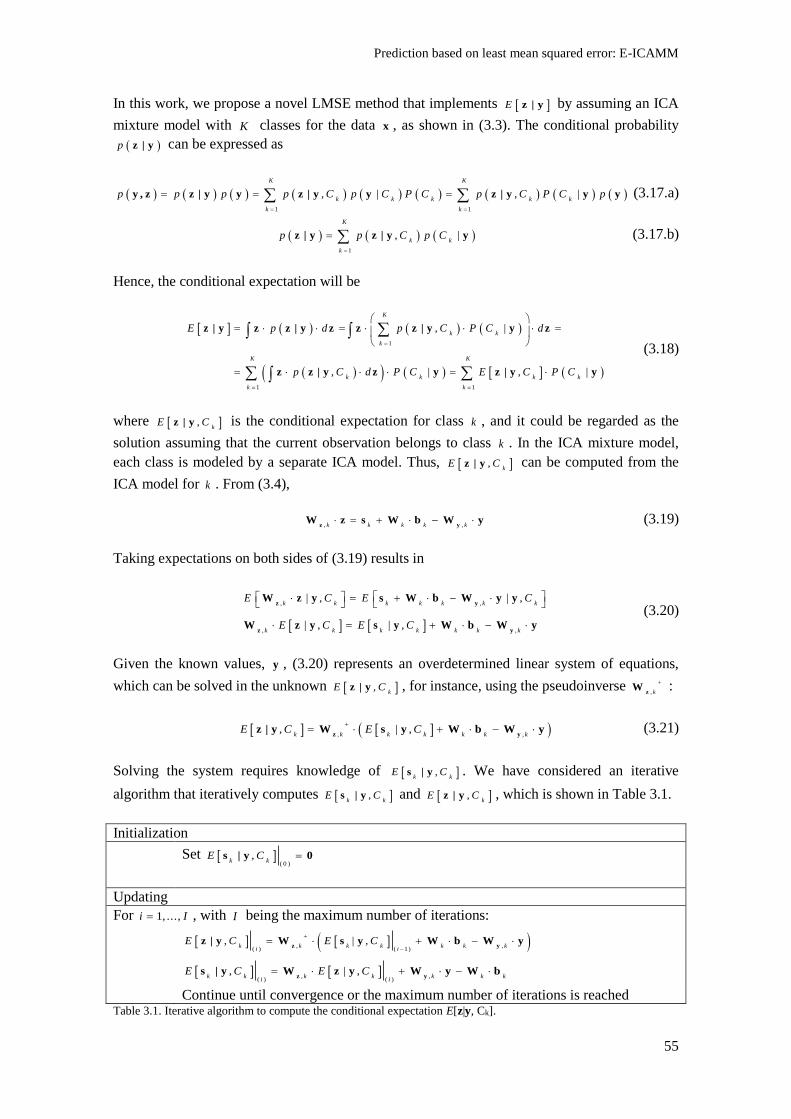
Prediction based on least mean squared error: E-ICAMM
55
In this work, we propose a novel LMSE method that implements E z | y by assuming an ICA
mixture model with K classes for the data x , as shown in (3.3). The conditional probability
p z | y can be expressed as
1 1
, | , |
K K
k k k k k
k k
p p p p C p C P C p C P C p
y , z z | y y z | y y z | y y y (3.17.a)
1
, |
K
k k
k
p p C p C
z | y z | y y (3.17.b)
Hence, the conditional expectation will be
1
1 1
, |
, | , |
K
k k
k
K K
k k k k
k k
E p d p C P C d
p C d P C E C P C
z | y z z | y z z z | y y z
z z | y z y z | y y
(3.18)
where ,k
E Cz | y is the conditional expectation for class k , and it could be regarded as the
solution assuming that the current observation belongs to class k . In the ICA mixture model,
each class is modeled by a separate ICA model. Thus, ,k
E Cz | y can be computed from the
ICA model for k . From (3.4),
, ,k k k k k
z yW z s W b W y (3.19)
Taking expectations on both sides of (3.19) results in
, ,
, ,
| , | ,
| , | ,
k k k k k k k
k k k k k k k
E C E C
E C E C
z y
z y
W z y s W b W y y
W z y s y W b W y
(3.20)
Given the known values, y , (3.20) represents an overdetermined linear system of equations,
which can be solved in the unknown ,k
E Cz | y , for instance, using the pseudoinverse , k
zW :
, ,, | ,
k k k k k k kE C E C
z yz | y W s y W b W y (3.21)
Solving the system requires knowledge of ,k k
E Cs | y . We have considered an iterative
algorithm that iteratively computes ,k k
E Cs | y and ,k
E Cz | y , which is shown in Table 3.1.
Initialization
Set ( 0 )
,k k
E C s | y 0
Updating
For 1, ...,i I , with I being the maximum number of iterations:
, ,
( ) ( 1 ), | ,
k k k k k k ki i
E C E C
z yz | y W s y W b W y
, ,( ) ( )
, | ,k k k k k k k
i iE C E C
z ys | y W z y W y W b
Continue until convergence or the maximum number of iterations is reached Table 3.1. Iterative algorithm to compute the conditional expectation E[z|y, Ck].
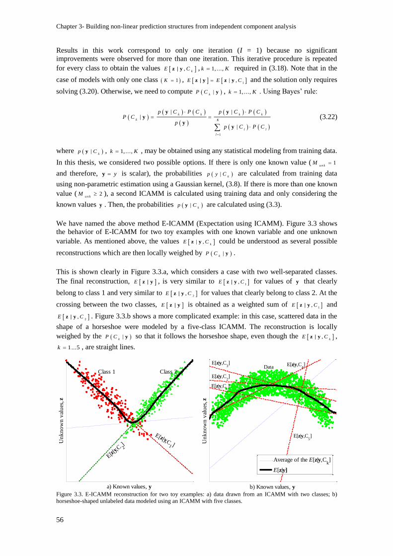
Chapter 3- Building non-linear prediction structures from independent component analysis
56
Results in this work correspond to only one iteration (I = 1) because no significant
improvements were observed for more than one iteration. This iterative procedure is repeated
for every class to obtain the values ,k
E Cz | y , 1, ...,k K required in (3.18). Note that in the
case of models with only one class 1K , 1| ,E E Cz | y z y and the solution only requires
solving (3.20). Otherwise, we need to compute |k
P C y , 1, ...,k K . Using Bayes’ rule:
1
| ||
|
k k k k
k K
l l
l
p C P C p C P CP C
pp C P C
y yy
yy
(3.22)
where |k
p Cy , 1, ...,k K , may be obtained using any statistical modeling from training data.
In this thesis, we considered two possible options. If there is only one known value ( 1u n k
M
and therefore, yy is scalar), the probabilities |k
p y C are calculated from training data
using non-parametric estimation using a Gaussian kernel, (3.8). If there is more than one known
value ( 2u n k
M ), a second ICAMM is calculated using training data and only considering the
known values y . Then, the probabilities |k
p Cy are calculated using (3.3).
We have named the above method E-ICAMM (Expectation using ICAMM). Figure 3.3 shows
the behavior of E-ICAMM for two toy examples with one known variable and one unknown
variable. As mentioned above, the values | ,k
E Cz y could be understood as several possible
reconstructions which are then locally weighed by |k
P C y .
This is shown clearly in Figure 3.3.a, which considers a case with two well-separated classes.
The final reconstruction, E z | y , is very similar to 1,E Cz | y for values of y that clearly
belong to class 1 and very similar to 2,E Cz | y for values that clearly belong to class 2. At the
crossing between the two classes, E z | y is obtained as a weighted sum of 1,E Cz | y and
2,E Cz | y . Figure 3.3.b shows a more complicated example: in this case, scattered data in the
shape of a horseshoe were modeled by a five-class ICAMM. The reconstruction is locally
weighed by the |k
P C y so that it follows the horseshoe shape, even though the ,k
E Cz | y ,
1...5k , are straight lines.
Figure 3.3. E-ICAMM reconstruction for two toy examples: a) data drawn from an ICAMM with two classes; b)
horseshoe-shaped unlabeled data modeled using an ICAMM with five classes.
a) Known values, y
Un
kn
ow
n v
alu
es,
z
Class 1 Class 2
E[z|y,C1 ]
E[z|y,
C 2]
b) Known values, y
Un
kn
ow
n v
alu
es,
z
Data
E[z|y,C1]
E[z|y,C2]
E[z|y,C3] E[z|y,C
4]
E[z|y,C5]
Average of the E[z|y,Ck]
E[z|y]
Prediction based on least mean squared error: E-ICAMM
57
3.2.1. Bias and local prediction error of E-ICAMM
Since it is the solution to the LMSE criterion, E-ICAMM is unbiased. This can be proved using
(3.18). If we denote the prediction error by ˆE IC A M M
E
e z z z z | y , then the bias is
the expected prediction error with respect to known and unknown data,
0E E E E E E E z ,y z y z z
e z z | y z z | y z z (3.23)
The mean squared error of the prediction can be obtained as the trace of the error covariance
matrix:
2
TT
T TT T
T TT
E E E E
E E E E E E E E
E E E E E E
z , y z , y
z , y z , y z , y z , y
z y
e e z z | y z z | y
z z z | y z z z | y z | y z | y
z z z z z | y z | y
(3.24)
One could also obtain the local mean squared error, i.e., the estimate of the prediction error of
E-ICAMM for any given set of observed values y. It is usually defined as the trace of the
conditional covariance with respect to known data, |T
E
e e y . Being an expectation, this
estimate is not likely to be a good indicator of the actual error of any one sample. However, this
error can be used to estimate the variability of the true values around the prediction yielded by
E-ICAMM, obtaining the prediction interval of E-ICAMM. This prediction interval can be used
to determine the quality of the prediction and identifying points that are likely to be badly
estimated.
Using the mixture model in (3.3), we can express |T
E
e e y as a combination of
| ,T
kE C
e e y , 1...k K :
1
1 1
| , |
, | | , |
K
T T T
k k
k
K K
T T
k k k k
k k
E p d p C P C d
p C d P C E C P C
e e y e e z | y z e e z | y y z
e e z | y z y e e y y
(3.25)
The local error for each class, | ,T
kE C
e e y , can be expressed as
| , | ,
, | | ,
| | , | | | ,
, , | | , |
TT
k k
TT
k k
TT
k k
T T TT
k k k
E C E E E C
E C E E C
E E C E E E C
E C E C E E E C E E
e e y z z | y z z | y y
z z | y z z y y
z y z y z y z y y
z z | y z | y z y z | y z y z | y z y
(3.26)
where |E z y is the E-ICAMM prediction and ,k
E Cz | y , 1, ...,k K , are obtained during
the process. The calculation of | ,T
kE C
z z y from (3.19) is straightforward, but complicated
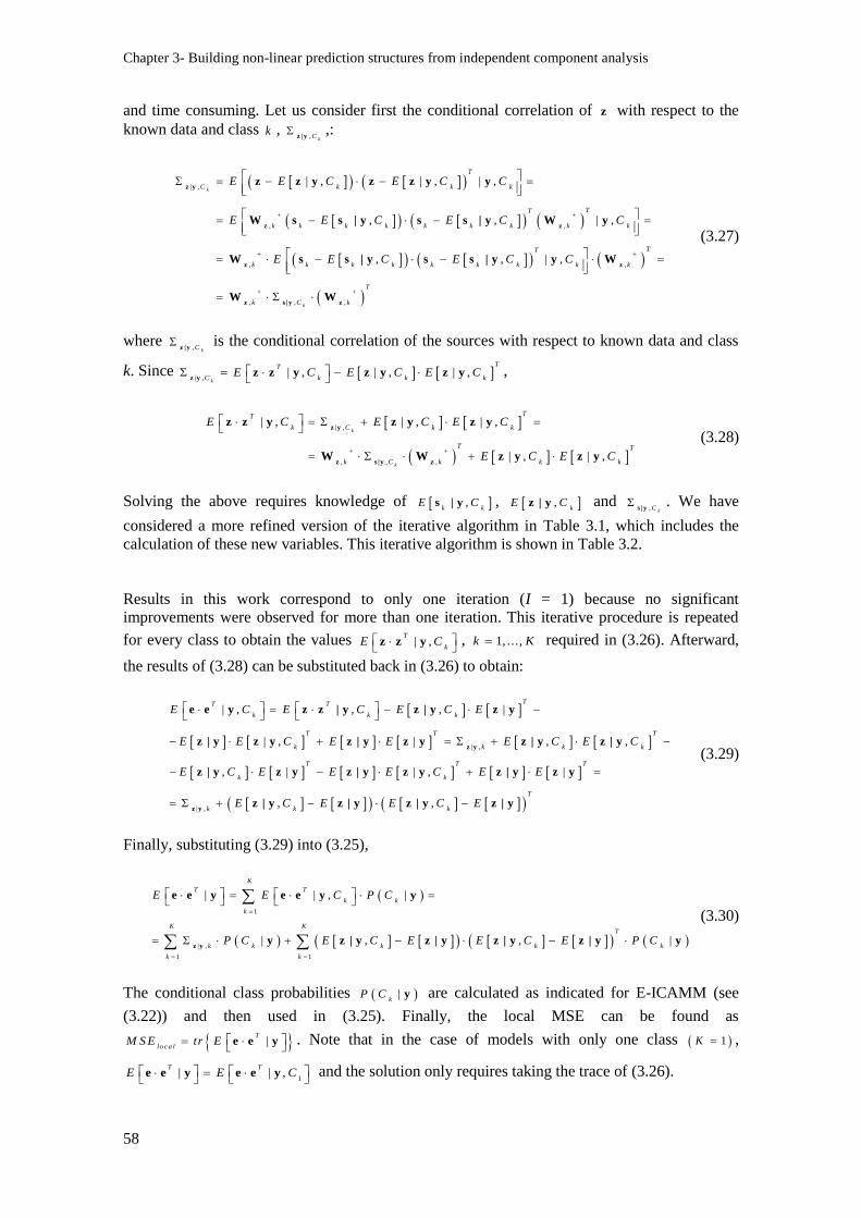
Chapter 3- Building non-linear prediction structures from independent component analysis
58
and time consuming. Let us consider first the conditional correlation of z with respect to the
known data and class k , ,
kC
z |y
,:
| ,
, ,
, ,
, , ,
| , | , | ,
, , | ,
, , | ,
k
k
T
C k k k
TT
k k k k k k k k k
TT
k k k k k k k k k
T
k C k
E E C E C C
E E C E C C
E E C E C C
z y
z z
z z
z s |y z
z z y z z y y
W s s | y s s | y W y
W s s | y s s | y y W
W W
(3.27)
where ,
kC
z |y
is the conditional correlation of the sources with respect to known data and class
k. Since | ,| , | , | ,
k
TT
C k k kE C E C E C z y
z z y z y z y ,
| ,
, , ,
| , | , | ,
| , | ,
k
k
TT
k C k k
T T
k C k k k
E C E C E C
E C E C
z y
z s |y z
z z y z y z y
W W z y z y
(3.28)
Solving the above requires knowledge of ,k k
E Cs | y , ,k
E Cz | y and ,
kC
s |y
. We have
considered a more refined version of the iterative algorithm in Table 3.1, which includes the
calculation of these new variables. This iterative algorithm is shown in Table 3.2.
Results in this work correspond to only one iteration (I = 1) because no significant
improvements were observed for more than one iteration. This iterative procedure is repeated
for every class to obtain the values | ,T
kE C
z z y , 1, ...,k K required in (3.26). Afterward,
the results of (3.28) can be substituted back in (3.26) to obtain:
| ,
| ,
| , , , |
| , | , ,
, | | , |
, ,
TT T
k k k
T T T
k k k k
T T T
k k
T
k k k
E C E C E C E
E E C E E E C E C
E C E E E C E E
E C E E C E
z y
z y
e e y z z | y z | y z y
z | y z y z | y z y z | y z | y
z | y z y z | y z y z | y z y
z | y z | y z | y z | y
(3.29)
Finally, substituting (3.29) into (3.25),
1
| ,
1 1
| | , |
| , , |
K
T T
k k
k
K KT
k k k k k
k k
E E C P C
P C E C E E C E P C
z y
e e y e e y y
y z | y z | y z | y z | y y
(3.30)
The conditional class probabilities |k
P C y are calculated as indicated for E-ICAMM (see
(3.22)) and then used in (3.25). Finally, the local MSE can be found as
|T
lo ca lM S E tr E
e e y . Note that in the case of models with only one class 1K ,
1| | ,
T TE E C e e y e e y and the solution only requires taking the trace of (3.26).
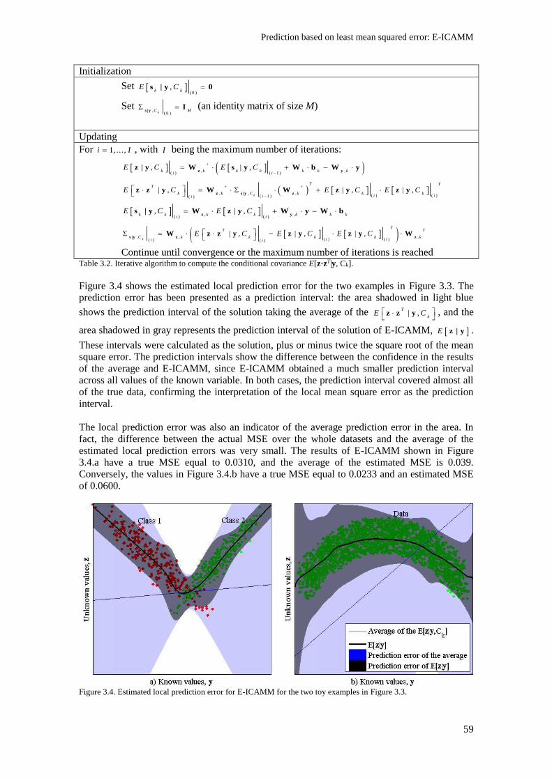
Prediction based on least mean squared error: E-ICAMM
59
Initialization
Set ( 0 )
,k k
E C s | y 0
Set ,
( 0 )kC M
s |y
I (an identity matrix of size M)
Updating
For 1, ...,i I , with I being the maximum number of iterations:
, ,
( ) ( 1 ), | ,
k k k k k k ki i
E C E C
z yz | y W s y W b W y
, , ,
( ) ( )( 1 )( )
| , | , | ,k
T TT
k k C k k ki iii
E C E C E C
z s |y z
z z y W W z y z y
, ,( ) ( )
, | ,k k k k k k k
i iE C E C
z ys | y W z y W y W b
, , ,
( )( ) ( )( )
| , | , | ,k ii
TT T
C k k k k kii
E C E C E C s |y z z
W z z y z y z y W
Continue until convergence or the maximum number of iterations is reached Table 3.2. Iterative algorithm to compute the conditional covariance E[z·zT|y, Ck].
Figure 3.4 shows the estimated local prediction error for the two examples in Figure 3.3. The
prediction error has been presented as a prediction interval: the area shadowed in light blue
shows the prediction interval of the solution taking the average of the | ,T
kE C
z z y , and the
area shadowed in gray represents the prediction interval of the solution of E-ICAMM, E z | y .
These intervals were calculated as the solution, plus or minus twice the square root of the mean
square error. The prediction intervals show the difference between the confidence in the results
of the average and E-ICAMM, since E-ICAMM obtained a much smaller prediction interval
across all values of the known variable. In both cases, the prediction interval covered almost all
of the true data, confirming the interpretation of the local mean square error as the prediction
interval.
The local prediction error was also an indicator of the average prediction error in the area. In
fact, the difference between the actual MSE over the whole datasets and the average of the
estimated local prediction errors was very small. The results of E-ICAMM shown in Figure
3.4.a have a true MSE equal to 0.0310, and the average of the estimated MSE is 0.039.
Conversely, the values in Figure 3.4.b have a true MSE equal to 0.0233 and an estimated MSE
of 0.0600.
Figure 3.4. Estimated local prediction error for E-ICAMM for the two toy examples in Figure 3.3.
Chapter 3- Building non-linear prediction structures from independent component analysis
60
3.3. Other methods
In this work, the proposed prediction methods are compared with several types of predictors.
These methods were selected due to their similarities to E-ICAMM or PREDICAMM, or due to
their application to real data (which will be shown in Chapter 5).
The first method selected for comparison was Kriging [116], which is a classical linear predictor
that is widely-used in geostatistics and other applications where the topographical distribution
of the signal is of importance. It was chosen because of this importance, and it was considered
both for simulated data and real data. Kriging is an implementation of the linear LMSE criterion
for spatial data, making it similar to E-ICAMM, which optimizes the LMSE criterion.
The second method for comparison was Wiener structures [278], a simple nonlinear prediction
method that is composed of a linear predictor followed by a nonlinear correction term. Wiener
structures have been used to successfully predict data from NDT applications [211], which is
the reason for their choosing. Wiener structures were used on simulated data and on real data.
The third considered method was matrix completion [36], a nonlinear method that estimates
missing data from a matrix from a few revealed entries. This method was chosen because of its
similarities with E-ICAMM and PREDICAMM, since it is an interpolator that considers
existing data and an underlying structure in order to reconstruct missing data. Given the
requirements of matrix completion (as explained in Section 3.3.3), it was considered only for
simulated data.
The fourth and last method for comparison was splines [69]. In splines, the data are usually
modeled using low-order polynomials that represent the lines or surfaces of lower energy. They
are a classic interpolation method. Furthermore, spherical splines are the typical interpolator for
electroencephalographic data [199], which is the reason why they were chosen for comparison
against E-ICAMM and PREDICAMM. Since they assume an underlying spherical structure,
spherical splines were only considered for their application on real data from an EEG
experiment, in Chapter 5. For non-EEG data, linear splines were used.
There are other methods that could be used for prediction, such as artificial neural networks
(ANN). However, previous works show that simpler methods (e.g., Wiener structures) can
model the nonlinearities in the data and obtain a good prediction at a lower computational cost
than ANN [222].
3.3.1. Kriging
Linear prediction is a fundamental tool in many different fields: adaptive filtering, system
identification, economics, geophysics, etc. [163]. It flows naturally from scenarios where one
can assume an underlying linear system, and it is optimal in those cases where the signals
follow Gaussian distributions.
Let us assume that there is a random stationary signal x n . The goal of linear prediction is to
estimate the value of the signal at time n l , x n l , from its last N values,
1 , 2 , ... ,x n x n x n N , where l is known as the “lag” in the prediction given by the
algorithm. Thus, the linear prediction can be written as
1
ˆ 1
N
T
i
i
x n l a x n i n
a x (3.31)
Other methods
61
where the vector 1 1 , 2 , ...,T
n x n x n x n N
x comprises known data and the
predictor's weights are included in vector 1 2, , ...,
T
Na a aa (super index T indicates matrix
transpose). Linear predictors are usually classified by their lag value; depending on l , we speak
of prediction 0l , interpolation 0l or regression 0l . The unknown parameters a are
usually optimized with respect to the mean squared error (MSE) between real values and
predicted values, resulting in the optimal values, o p t
a . In this case, the cost function, J a , is
2
2ˆ1 1 1J E x n x n E e n
a (3.32)
where e n is the prediction error. The gradient of the cost function can be used to find an
optimal set of parameters, o p t
a . Assuming stationary Normally-distributed data, this process will
result in the Wiener-Hopf equations [236]:
, 0x o p t x
R a r (3.33)
0 1 1
1 0 2
1 2 0
x x x
x x x
x
x x x
r r r N
r r r N
r N r N r
R (3.34.a)
, 01 , 2 , ...,
T
x x x xr l r l r l N
r (3.34.b)
where x
R is the covariance matrix of signal x n , , 0x
r is its covariance vector, and xr is
the covariance function for lag . Assuming that the covariance matrix is nonsingular, the
optimal linear predictor can be calculated by inverting x
R ,
1
, 0o p t x x
a R r (3.35)
Since x
R is a Toeplitz matrix (each descending diagonal from left to right is constant), the
system of equations (3.33) can be solved efficiently by using the classical Levinson-Durbin
algorithm [155].
Geostatistics is a field where linear predictors show a large presence. One of the most important
algorithms in this area is Kriging, a linear interpolator that calculates o p t
a using the spatial
covariance of data [116]. The original algorithm, Simple Kriging, is similar to a 2-D linear
predictor. Thus, equation (3.31) becomes
0
1
N
T
i i
i
x a x
p p a x (3.36)
where i
p is the position of the -thi data point, ix p , and 1 2
, , ...,T
Nx x x
x p p p .
Typically, only the N nearest positions are chosen for prediction, or N is equal to the number
of points within a certain distance of the unknown data point. Equations (3.34.a) and (3.34.b)
are modified to include the spatial distribution of 0x p :
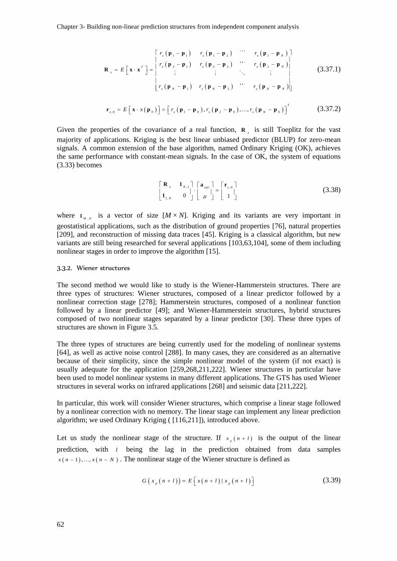
Chapter 3- Building non-linear prediction structures from independent component analysis
62
1 1 1 2 1
2 1 2 2 2
1 2
x x x N
x x x NT
x
x N x N x N N
r r r
r r rE
r r r
p p p p p p
p p p p p pR x x
p p p p p p
(3.37.1)
, 0 0 1 0 2 0 0, , ...,
T
x x x x NE x r r r
r x p p p p p p p (3.37.2)
Given the properties of the covariance of a real function, x
R is still Toeplitz for the vast
majority of applications. Kriging is the best linear unbiased predictor (BLUP) for zero-mean
signals. A common extension of the base algorithm, named Ordinary Kriging (OK), achieves
the same performance with constant-mean signals. In the case of OK, the system of equations
(3.33) becomes
,1 ,0
1,0 1
x N o p t x
N
R 1 a r
1 (3.38)
where ,M N
1 is a vector of size [M × N]. Kriging and its variants are very important in
geostatistical applications, such as the distribution of ground properties [76], natural properties
[209], and reconstruction of missing data traces [45]. Kriging is a classical algorithm, but new
variants are still being researched for several applications [103,63,104], some of them including
nonlinear stages in order to improve the algorithm [15].
3.3.2. Wiener structures
The second method we would like to study is the Wiener-Hammerstein structures. There are
three types of structures: Wiener structures, composed of a linear predictor followed by a
nonlinear correction stage [278]; Hammerstein structures, composed of a nonlinear function
followed by a linear predictor [49]; and Wiener-Hammerstein structures, hybrid structures
composed of two nonlinear stages separated by a linear predictor [30]. These three types of
structures are shown in Figure 3.5.
The three types of structures are being currently used for the modeling of nonlinear systems
[64], as well as active noise control [288]. In many cases, they are considered as an alternative
because of their simplicity, since the simple nonlinear model of the system (if not exact) is
usually adequate for the application [259,268,211,222]. Wiener structures in particular have
been used to model nonlinear systems in many different applications. The GTS has used Wiener
structures in several works on infrared applications [268] and seismic data [211,222].
In particular, this work will consider Wiener structures, which comprise a linear stage followed
by a nonlinear correction with no memory. The linear stage can implement any linear prediction
algorithm; we used Ordinary Kriging ( [116,211]), introduced above.
Let us study the nonlinear stage of the structure. If px n l is the output of the linear
prediction, with l being the lag in the prediction obtained from data samples
1 , .. . ,x n x n N . The nonlinear stage of the Wiener structure is defined as
|p p
G x n l E x n l x n l
(3.39)
Other methods
63
Figure 3.5. Wiener structure (top), Hammerstein structure (middle), and Wiener-Hammerstein structure (bottom).
Thus, the nonlinearity implemented by the Wiener structure, G , is the conditional
expectation of real data with respect to the output of the linear predictor. Assuming that x n is
stationary, G can be estimated from the signal. This estimation can be done in many ways,
but we considered two methods: direct sample estimation and polynomial approximation (
[268]).
3.3.2.a. Direct sample estimation
The nonlinear function G can be estimated by applying a sliding window on a set of training
data:
1
1i
p i l
i
G i w i
x x (3.40)
where p
x is a vector with the output values of the linear predictor, sorted from lower to higher;
lx is a vector with the real data values that correspond to those same values (and, thus, sorted in
the same way as p
x ); and i
w is the -thi value of the sliding window of length . This
estimation will return a finite set of points – the curve G is interpolated from this set.
In this work, all instances of direct sample estimation were done using a rectangular window of
length 21 . This value was selected rather heuristically using several experiments with
simulated data, using the same experiments shown later in this Chapter.
3.3.2.b. Polynomial approximation
A one-dimensional approximation of the nonlinear stage of the Wiener structure was presented
in [268]. Assuming that px n is a Gaussian sequence with zero mean and normalized
variance, and taking p px n l x and x n l x for convenience of notation:
Linear
predictor
Linear
predictor
Linear
predictor
Zero-memory
nonlinearity
Zero-memory
nonlinearity
Zero-memory
nonlinearity Zero-memory
nonlinearity
x
x
x
x(n-1) x(n-2)
.
.
. x(n-N)
x(n-1) x(n-2)
.
.
. x(n-N)
x(n-1) x(n-2)
.
.
. x(n-N)
x(n)
x(n)
x(n)
^
^
^
Chapter 3- Building non-linear prediction structures from independent component analysis
64
1
1,
!p m p m p
m
G x C x x H xm
(3.41)
where m
C is the cross cumulant, defined as
t im e s
, , , . . . ,
m
mC x y c u m u la n t x y y
and m
H is the
-thm order Hermite polynomial. The assumption of Gaussianity is not as restrictive as it might
seem, since px n is the output of a linear predictor – thus, for a large enough N , the Central
Limit Theorem ensures the Gaussianity of the data. In previous works, we have found that the
series can be truncated at the third term [268]. In that case, the result is:
3 2
3 3 1 2 1 3 2
1 1 5 1 13
6 2 2 2 2p p p p
G x a a x a x a a x a
(3.42)
where i
i pa E x x
are the cross-moments, estimated from training data.
3.3.3. Matrix completion based on smoothed rank function (SRF)
In many practical problems, one would like to recover a matrix from a sampling of its entries;
for instance, one could attempt to infer the answers in a partially-answered survey (this is also
known as the “Netflix problem”). Matrix completion consist in the reconstruction of these
missing entries from known data by assuming that the matrix is structured, i.e., it has low rank
[36]. It can be regarded as an extension of compressed sensing, since it shows that many objects
or structures, and not only sparse signals and images, can be reconstructed from a limited set of
measurements.
Consider a matrix M of which only a few entries are known. We would like to recover the
whole matrix based on these revealed entries; however, it is clear that solving this problem is
not possible without any additional information. Now, let us assume that the matrix is of
dimension 1 2n n and its rank is r ; it is straightforward to calculate that the number of
degrees of freedom of this matrix is equal to 1 2r n n r . So, in order to exactly recover the
matrix, it is necessary that the number of revealed entries is larger than this number of degrees
of freedom. In fact, recovery of the matrix from a small number of known entries is possible as
long as the matrix is low-rank and entries are selected uniformly [36]. In brief, the objetive of
matrix completion is to obtain a matrix with minimum rank, given a subset of its entries.
There are many matrix completion algorithms, such as FPCA [97] and SDP [81]. In this work,
we considered an algorithm based on a smoothed rank function (SRF) [95], which makes use of
a continuous and differentiable approximation of the discontinuous rank function. This function
can then be minimized using any classical optimization technique.
Consider an unknown matrix M of dimension 1 2n n and rank r for which only m entries
have been revealed. Assume that m is sufficiently large and the locations of the observed
entries are sufficiently uniformly distributed; in that case, the matrix completion problem is to
find a matrix o p t
X that solves the optimization problem:
m in
. . , ,ij ij
ra n k
s t X M i j
X
(3.43)
Other methods
65
where is the set of locations corresponding to the m observed entries. SRF uses a
continuous approximation F of the rank function and then applies continuous optimization
techniques to minimize it. One such function is the Gaussian function:
2 2/ 2
1
k
n
k
F n e
X
X (3.44)
where is a parameter, k X is the -thk singular value of X , and 1 2
m in ,n n n . As
approaches zero, F
approaches the rank function. Equation (3.44) is minimized using any
gradient algorithm while enforcing the condition , ,i j i j
X M i j .
3.3.4. Splines
Splines are smooth polynomial curves that are piecewise-defined, and are smooth at the
connections between pieces [69]. The highest order of the piecewise polynomials is the order of
the spline. Splines can obtain good results even with low orders. For instance, the most
commonly-used splines are cubic splines, which are of order 3. The smooth curve obtained by
splines can be used for many purposes, one of them being data interpolation, since it can be
used to evaluate the fitted function at new points. The term “spline” was adopted from the name
of a flexible strip of metal commonly used by draftsmen to assist in drawing curved lines. This
strip was held in place at several points or “knots,” and the strip would adopt the shape of
minimum strain energy between knots.
Let us assume that we have a set of measurements jz y at prescribed points
jy , 1 ...j N .
Briefly, cubic splines fit a piecewise function of the form
1 1 2
2 2 3
1 1
, i f y
, if
, i f N N N
p y y y
p y y y yP y
p y y y y
(3.45)
to the measurements, where i
p is the 3rd -degree polynomial 3 2
i i i i ip y a y b y c y d
for the -thi piece, 1... 1i N . The coefficients , , ,i i i i
a b c d of the piecewise polynomial are
calculated such that: a) P y and its first two derivatives are continuous in the range 1,
Ny y ;
b) the piecewise function is exactly equal to the observed value at each one of the nodes, that is,
, 1 ...j j
P y z y j N .
3.3.4.a. Thin-plate splines
Thin-plate splines (TPS) are a generalization of splines to two or more dimensions [74]. TPS
can be likened to the bending of a thin sheet of metal; just like the metal has rigidity, the thin-
plate splines also resist bending by setting a penalty involving the smoothness of the fitted
surface.
Let us assume that we have a set of measurements, iz y , at prescribed coordinates
jy ,
1 ...j N . The thin-plate spline f y is obtained by minimizing the cost function
1p E p R f f , where E f measures the fitting error, R f measures the roughness
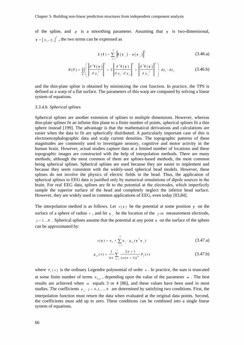
Chapter 3- Building non-linear prediction structures from independent component analysis
66
of the spline, and p is a smoothing parameter. Assuming that y is two-dimensional,
1 2,
T
y yy , the two terms can be expressed as
2
1
N
j j
j
E
f f y z y (3.46.a)
2
2 2 22 2 2
1 22 2
1 1 2 2
2R d y d yy y y y
f y f y f y
f (3.46.b)
and the thin-plate spline is obtained by minimizing the cost function. In practice, the TPS is
defined as a warp of a flat surface. The parameters of this warp are computed by solving a linear
system of equations.
3.3.4.b. Spherical splines
Spherical splines are another extension of splines to multiple dimensions. However, whereas
thin-plate splines fit an infinite thin plane to a finite number of points, spherical splines fit a thin
sphere instead [199]. The advantage is that the mathematical derivations and calculations are
easier when the data to fit are spherically distributed. A particularly important case of this is
electroencephalographic data and scalp current densities. The topographic patterns of these
magnitudes are commonly used to investigate sensory, cognitive and motor activity in the
human brain. However, actual studies capture data at a limited number of locations and these
topographic images are constructed with the help of interpolation methods. There are many
methods, although the most common of them are splines-based methods, the most common
being spherical splines. Spherical splines are used because they are easier to implement and
because they seem consistent with the widely-used spherical head models. However, these
splines do not involve the physics of electric fields in the head. Thus, the application of
spherical splines to EEG data is justified only by numerical simulations of dipole sources in the
brain. For real EEG data, splines are fit to the potential at the electrodes, which imperfectly
sample the superior surface of the head and completely neglect the inferior head surface.
However, they are widely used in common applications of EEG, even today [83,84].
The interpolation method is as follows. Let z y be the potential at some position y on the
surface of a sphere of radius r , and let j
y be the location of the -thj measurement electrode,
1 ...j N . Spherical splines assume that the potential at any point y on the surface of the sphere
can be approximated by:
0
1
( ) ( )
N
j j
j
T
mz a a g
y y y (3.47.a)
1
2 1
( ( 1)
1( ) ( )
4 )m nm
n
nxg
nxP
n
(3.47.b)
where nP x is the ordinary Legendre polynomial of order n . In practice, the sum is truncated
at some finite number of terms m ax
n , depending upon the value of the parameter m . The best
results are achieved when m equals 3 or 4 [86], and these values have been used in most
studies. The coefficients , 0 ,1, .. . ,j
a j N are determined by satisfying two conditions. First, the
interpolation function must return the data when evaluated at the original data points. Second,
the coefficients must add up to zero. These conditions can be combined into a single linear
system of equations.
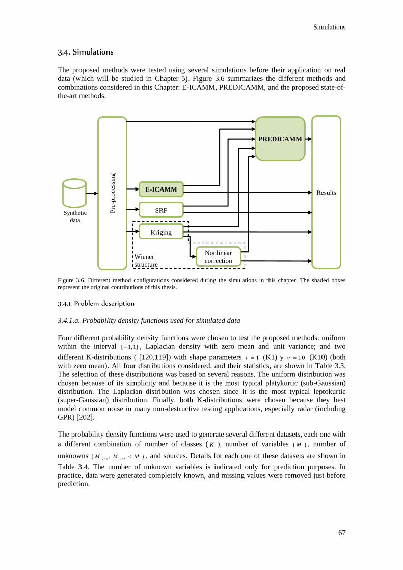
Simulations
67
3.4. Simulations
The proposed methods were tested using several simulations before their application on real
data (which will be studied in Chapter 5). Figure 3.6 summarizes the different methods and
combinations considered in this Chapter: E-ICAMM, PREDICAMM, and the proposed state-of-
the-art methods.
Figure 3.6. Different method configurations considered during the simulations in this chapter. The shaded boxes
represent the original contributions of this thesis.
3.4.1. Problem description
3.4.1.a. Probability density functions used for simulated data
Four different probability density functions were chosen to test the proposed methods: uniform
within the interval [ 1,1] , Laplacian density with zero mean and unit variance; and two
different K-distributions ( [120,119]) with shape parameters 1 (K1) y 10 (K10) (both
with zero mean). All four distributions considered, and their statistics, are shown in Table 3.3.
The selection of these distributions was based on several reasons. The uniform distribution was
chosen because of its simplicity and because it is the most typical platykurtic (sub-Gaussian)
distribution. The Laplacian distribution was chosen since it is the most typical leptokurtic
(super-Gaussian) distribution. Finally, both K-distributions were chosen because they best
model common noise in many non-destructive testing applications, especially radar (including
GPR) [202].
The probability density functions were used to generate several different datasets, each one with
a different combination of number of classes ( K ), number of variables M , number of
unknowns ,u n k u n k
M M M , and sources. Details for each one of these datasets are shown in
Table 3.4. The number of unknown variables is indicated only for prediction purposes. In
practice, data were generated completely known, and missing values were removed just before
prediction.
Pre
-pro
cess
ing
Results
Synthetic
data
PREDICAMM
E-ICAMM
SRF
Kriging
Nonlinear
correction Wiener
structure

Chapter 3- Building non-linear prediction structures from independent component analysis
68
Probability density
function
Skewness Kurtosis Plot
Uniform 0 -1.2 (platykurtic)
Laplacian 0 3 (leptokurtic)
K1 1.7 5.3 (leptokurtic)
K10 0.8 0.7 (leptokurtic)
Table 3.3. Data distributions used for simulation.
Dataset # of
classes, K
# of
variables,
M
# of
unknown
variables,
Munk
Probability density
functions of the sources,
p(sk)
Single-class
datasets
1 1 2 1 Uniform, Laplacian
2 1 3 1 Uniform, Laplacian, K1
3 1 4 2 Uniform, Laplacian, K1, K10
4 1 4 2 Uniform
5 1 4 2 Laplacian
Multiple-
class datasets
6 2 3 1 Uniform, Laplacian
7 2 4 2 Uniform, Laplacian
8 2 4 2 Laplacian, K1
9 2 4 2 K1, K10
10 3 3 1 Uniform, Laplacian, K1
11 3 4 2 Uniform, Laplacian, K1
12 3 3 1 Uniform, Laplacian, K1, K10
13 3 4 2 Uniform, Laplacian, K1, K10 Table 3.4. Details of all datasets used in the simulated experiment.
3.4.1.b. Parameter estimation
During each iteration of the experiments, the generated data were split 50/50 into training and
test, as shown in Figure 3.7. The training data were used to estimate the parameters of each of
the proposed methods using supervised training.
E-ICAMM and PREDICAMM require the estimation of the ICAMM parameters,
, , ,k k k
pW s b 1...k K . These parameters were estimated using supervised training with the
MIXCA procedure [231] with JADE as the embedded ICA method. Prediction was performed
using the sampling scheme shown in Figure 3.1.a. As mentioned in Section 3.1.1, the selection
of the initial value for PREDICAMM is very important, as is the selection of the gradient
algorithm. These values were set experimentally, and the results are shown in Section 3.4.3.
For Kriging, the data were treated as if the description in Figure 3.7 was a two-dimensional
problem, and the -thm value of the -thn observation was denoted as , ,T
x m np p . The
covariance matrix and the covariance vector (x
R and ,0x
r respectively) were estimated using
the sample spatial covariance calculated from training data, and each unknown position was
reconstructed using all the known positions within a distance of K r ig
M samples. This value was
chosen empirically.
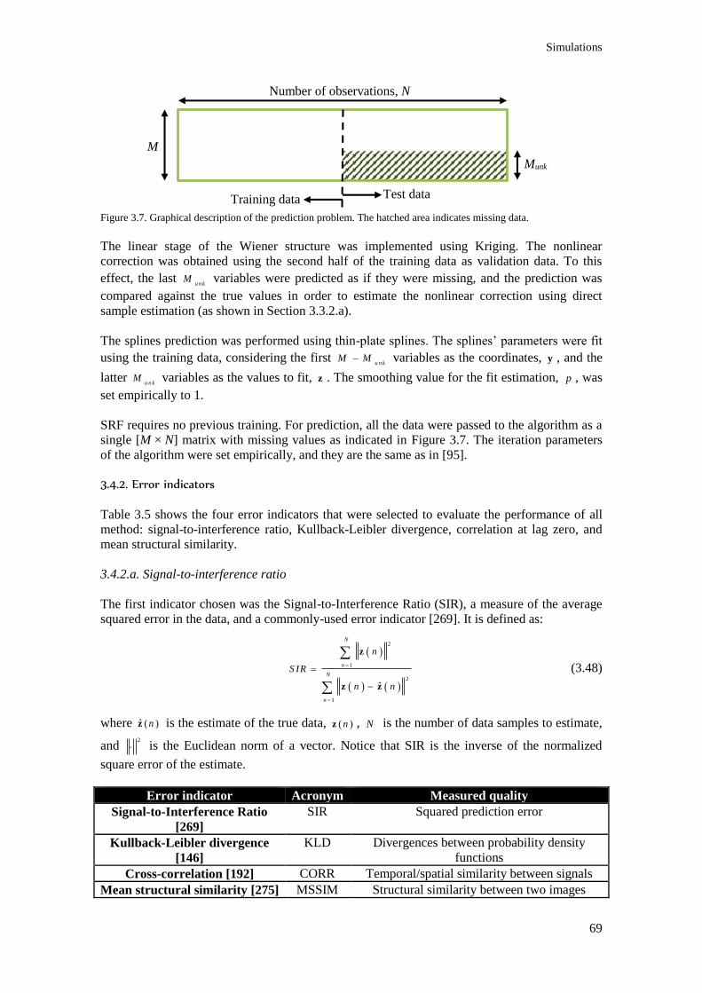
Simulations
69
Figure 3.7. Graphical description of the prediction problem. The hatched area indicates missing data.
The linear stage of the Wiener structure was implemented using Kriging. The nonlinear
correction was obtained using the second half of the training data as validation data. To this
effect, the last u n k
M variables were predicted as if they were missing, and the prediction was
compared against the true values in order to estimate the nonlinear correction using direct
sample estimation (as shown in Section 3.3.2.a).
The splines prediction was performed using thin-plate splines. The splines’ parameters were fit
using the training data, considering the first u n k
M M variables as the coordinates, y , and the
latter u n k
M variables as the values to fit, z . The smoothing value for the fit estimation, p , was
set empirically to 1.
SRF requires no previous training. For prediction, all the data were passed to the algorithm as a
single [M × N] matrix with missing values as indicated in Figure 3.7. The iteration parameters
of the algorithm were set empirically, and they are the same as in [95].
3.4.2. Error indicators
Table 3.5 shows the four error indicators that were selected to evaluate the performance of all
method: signal-to-interference ratio, Kullback-Leibler divergence, correlation at lag zero, and
mean structural similarity.
3.4.2.a. Signal-to-interference ratio
The first indicator chosen was the Signal-to-Interference Ratio (SIR), a measure of the average
squared error in the data, and a commonly-used error indicator [269]. It is defined as:
2
1
2
1
ˆ
N
n
N
n
n
S IR
n n
z
z z
(3.48)
where ˆ ( )nz is the estimate of the true data, ( )nz , N is the number of data samples to estimate,
and 2
is the Euclidean norm of a vector. Notice that SIR is the inverse of the normalized
square error of the estimate.
Error indicator Acronym Measured quality
Signal-to-Interference Ratio
[269]
SIR Squared prediction error
Kullback-Leibler divergence
[146]
KLD Divergences between probability density
functions
Cross-correlation [192] CORR Temporal/spatial similarity between signals
Mean structural similarity [275] MSSIM Structural similarity between two images
Test data Training data
M
Munk
Number of observations, N
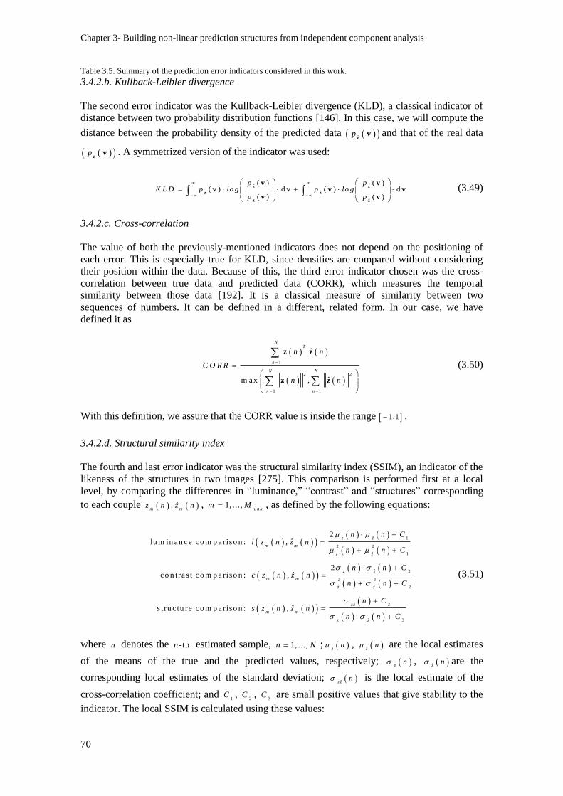
Chapter 3- Building non-linear prediction structures from independent component analysis
70
Table 3.5. Summary of the prediction error indicators considered in this work.
3.4.2.b. Kullback-Leibler divergence
The second error indicator was the Kullback-Leibler divergence (KLD), a classical indicator of
distance between two probability distribution functions [146]. In this case, we will compute the
distance between the probability density of the predicted data ˆp
zv and that of the real data
pz
v . A symmetrized version of the indicator was used:
ˆ
ˆ
ˆ
( ) ( )( ) d ( ) d
( ) ( )
p pK L D p lo g p lo g
p p
z z
z z
z z
v vv v v v
v v (3.49)
3.4.2.c. Cross-correlation
The value of both the previously-mentioned indicators does not depend on the positioning of
each error. This is especially true for KLD, since densities are compared without considering
their position within the data. Because of this, the third error indicator chosen was the cross-
correlation between true data and predicted data (CORR), which measures the temporal
similarity between those data [192]. It is a classical measure of similarity between two
sequences of numbers. It can be defined in a different, related form. In our case, we have
defined it as
1
2 2
1 1
ˆ
ˆm a x ,
NT
n
N N
n n
n n
C O R R
n n
z z
z z
(3.50)
With this definition, we assure that the CORR value is inside the range 1,1 .
3.4.2.d. Structural similarity index
The fourth and last error indicator was the structural similarity index (SSIM), an indicator of the
likeness of the structures in two images [275]. This comparison is performed first at a local
level, by comparing the differences in “luminance,” “contrast” and “structures” corresponding
to each couple ˆ,m m
z n z n , 1, ...,u n k
m M , as defined by the following equations:
ˆ
ˆ
1
2 2
1
ˆ 2
2 2
ˆ 2
ˆ 3
ˆ 3
ˆ
ˆlu m in a n c e c o m p a riso n : ,
ˆ,
2
2c o n tra s t c o m p a riso n :
s tru c tu re c o m p a riso n : ˆ ,
z z
m m
z z
z
m m
z
m
z
zz
z
m
z
z
n nl z n z n
n n
n nz n z n
n n
nz n z n
C
C
Cc
C
Cs
Cn n
(3.51)
where n denotes the -thn estimated sample, 1, ...,n N ; zn , z
n are the local estimates
of the means of the true and the predicted values, respectively; zn , z
n are the
corresponding local estimates of the standard deviation; ˆz zn is the local estimate of the
cross-correlation coefficient; and 1
C , 2
C , 3
C are small positive values that give stability to the
indicator. The local SSIM is calculated using these values:

Simulations
71
ˆ ˆ ˆ ˆ, , · , · ,m m m m m m m m
S S IM z n z n l z n z n c z n z n s z n z n
(3.52)
where , , are parameters that set the relative importance of each term. In this work, we
consider 1 , 1
/ 1 0 0C R , 2
* 3 / 1 0C R and 3 2
/ 2C C (where R is the dynamic
range of the true values). The mean SSIM (or MSSIM) between two images is the average of all
the local SSIM
1 1
1 1ˆ,
u n kM N
m m
m nu n k
M S S IM S S IM z n z nN M
(3.53)
3.4.2.e. Relative importance
The relative importance of these error indicators depends on the application. SIR would be the
most common, given that most algorithms attempt to minimize the mean squared error, which is
equivalent to maximizing the SIR. It is a good general indicator of the prediction performance,
perhaps the most important in applications where a low error is needed. It is quite popular in
blind-source separation applications, in order to estimate the goodness of the recovered sources
[276,35].
KLD would be more important in applications where the resulting density of predicted data is a
factor, e.g., a predictor that was a pre-processing step to an algorithm that depends on the
probability density function of the data. It is also quite popular in pattern recognition
applications, and even more so in speech processing [242] and image processing [96]. The best
possible value for the KLD is zero (it being a distance), unlike the other considered error
indicators.
CORR is important in applications where the spatial or temporal structure of predicted data
must be preserved. It is a robust measure of the temporal synchronicity between two signals and
it can be reliably estimated from sample data. CORR is a popular method for the determination
of the distance between two sets of neuron spike trains [238,193].
MSSIM is a common error indicator in the field of image processing. Unlike other error
evaluation methods, MSSIM is based on a model of the human visual system (HVS), a fact that
allows it to better estimate the perceived quality of processed images [275,274]. It has been used
for evaluating image processing results in several applications, such as image watermarking [5]
and radar imaging [21].
3.4.3. Parameter setting for PREDICAMM
3.4.3.a. Convergence analysis
The study of the convergence of PREDICAMM was conducted in an empirical fashion, using
exhaustive search with Monte Carlo experiments. The data for each iteration of the experiment
were simulated using an ICAMM whose sources followed one or more of the considered
datasets shown in Table 3.4; class parameters k
W , kp s and
kb were randomly set for each
class, and all classes were assumed to be equiprobable. This model was used to generate 1,000
observations. As explained in Section 3.4.1, the first half of these observations was used to
estimate the ICAMM parameters using supervised training. The second half of the observations
was used to test the prediction performance of PREDICAMM. The Monte Carlo experiment
comprised 100 iterations, with the end result being the average of all partial results. This process
is shown in Figure 3.8.
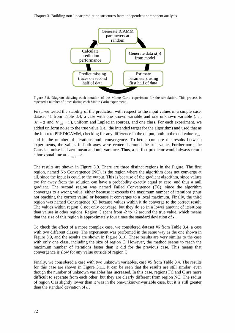
Chapter 3- Building non-linear prediction structures from independent component analysis
72
Figure 3.8. Diagram showing each iteration of the Monte Carlo experiment for the simulation. This process is
repeated a number of times during each Monte Carlo experiment.
First, we tested the stability of the prediction with respect to the input values in a simple case,
dataset #1 from Table 3.4; a case with one known variable and one unknown variable (i.e.,
2M and 1u n k
M ), uniform and Laplacian sources, and one class. For each experiment, we
added uniform noise to the true value (i.e., the intended target for the algorithm) and used that as
the input to PREDICAMM, checking for any difference in the output, both in the end value e n d
z
and in the number of iterations until convergence. To better compare the results between
experiments, the values in both axes were centered around the true value. Furthermore, the
Gaussian noise had zero mean and unit variance. Thus, a perfect predictor would always return
a horizontal line at
0e n d
z .
The results are shown in Figure 3.9. There are three distinct regions in the Figure. The first
region, named No Convergence (NC), is the region where the algorithm does not converge at
all, since the input is equal to the output. This is because of the gradient algorithm, since values
too far away from the solution can have a probability exactly equal to zero, and thus a null
gradient. The second region was named Failed Convergence (FC), since the algorithm
converges to a wrong value, either because it exceeds the maximum number of iterations (thus
not reaching the correct value) or because it converges to a local maximum. Finally, the third
region was named Convergence (C) because values within it do converge to the correct result.
The values within region C not only converge, but they do so in a lower amount of iterations
than values in other regions. Region C spans from -2 to +2 around the true value, which means
that the size of this region is approximately four times the standard deviation of x .
To check the effect of a more complex case, we considered dataset #6 from Table 3.4, a case
with two different classes. The experiment was performed in the same way as the one shown in
Figure 3.9, and the results are shown in Figure 3.10. These results are very similar to the case
with only one class, including the size of region C. However, the method seems to reach the
maximum number of iterations faster than it did for the previous case. This means that
convergence is slow for any value outside of region C.
Finally, we considered a case with two unknown variables, case #5 from Table 3.4. The results
for this case are shown in Figure 3.11. It can be seen that the results are still similar, even
though the number of unknown variables has increased. In this case, regions FC and C are more
difficult to separate from each other, but they are clearly different from region NC. The radius
of region C is slightly lower than it was in the one-unknown-variable case, but it is still greater
than the standard deviation of x .
Generate ICAMM parameters at
random
Generate data x(n) from model
Estimate parameters using first half of data
Predict missing traces on second
half of data
Calculate prediction
performance
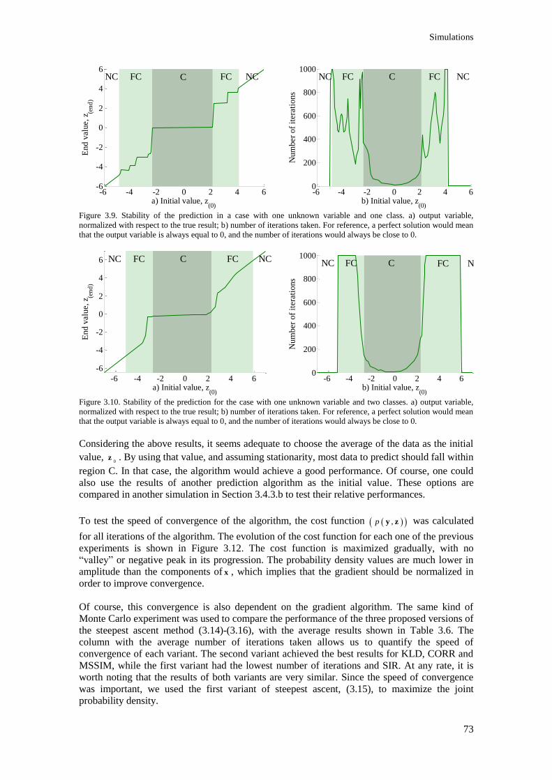
Simulations
73
Figure 3.9. Stability of the prediction in a case with one unknown variable and one class. a) output variable,
normalized with respect to the true result; b) number of iterations taken. For reference, a perfect solution would mean
that the output variable is always equal to 0, and the number of iterations would always be close to 0.
Figure 3.10. Stability of the prediction for the case with one unknown variable and two classes. a) output variable,
normalized with respect to the true result; b) number of iterations taken. For reference, a perfect solution would mean
that the output variable is always equal to 0, and the number of iterations would always be close to 0.
Considering the above results, it seems adequate to choose the average of the data as the initial
value, 0
z . By using that value, and assuming stationarity, most data to predict should fall within
region C. In that case, the algorithm would achieve a good performance. Of course, one could
also use the results of another prediction algorithm as the initial value. These options are
compared in another simulation in Section 3.4.3.b to test their relative performances.
To test the speed of convergence of the algorithm, the cost function ,p y z was calculated
for all iterations of the algorithm. The evolution of the cost function for each one of the previous
experiments is shown in Figure 3.12. The cost function is maximized gradually, with no
“valley” or negative peak in its progression. The probability density values are much lower in
amplitude than the components of x , which implies that the gradient should be normalized in
order to improve convergence.
Of course, this convergence is also dependent on the gradient algorithm. The same kind of
Monte Carlo experiment was used to compare the performance of the three proposed versions of
the steepest ascent method (3.14)-(3.16), with the average results shown in Table 3.6. The
column with the average number of iterations taken allows us to quantify the speed of
convergence of each variant. The second variant achieved the best results for KLD, CORR and
MSSIM, while the first variant had the lowest number of iterations and SIR. At any rate, it is
worth noting that the results of both variants are very similar. Since the speed of convergence
was important, we used the first variant of steepest ascent, (3.15), to maximize the joint
probability density.
-6 -4 -2 0 2 4 6-6
-4
-2
0
2
4
6
a) Initial value, z(0)
En
d v
alu
e, z
(en
d)
NC NCFC FCC
-6 -4 -2 0 2 4 60
200
400
600
800
1000
b) Initial value, z(0)
Nu
mb
er o
f it
era
tio
ns
C NCNC FCFC
-6 -4 -2 0 2 4 6
-6
-4
-2
0
2
4
6
a) Initial value, z(0)
End v
alu
e, z (e
nd
)
C NCNC FCFC
-6 -4 -2 0 2 4 60
200
400
600
800
1000
b) Initial value, z(0)
Num
ber
of
itera
tions
FCFC NCNC C
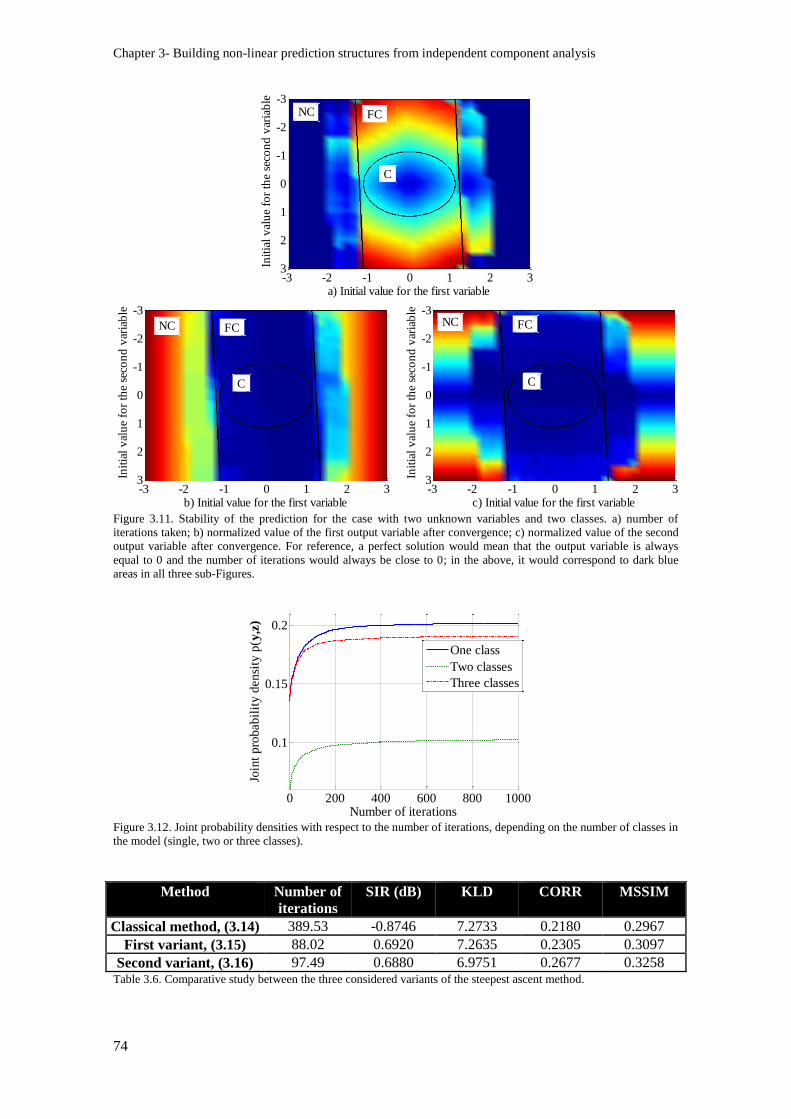
Chapter 3- Building non-linear prediction structures from independent component analysis
74
Figure 3.11. Stability of the prediction for the case with two unknown variables and two classes. a) number of
iterations taken; b) normalized value of the first output variable after convergence; c) normalized value of the second
output variable after convergence. For reference, a perfect solution would mean that the output variable is always
equal to 0 and the number of iterations would always be close to 0; in the above, it would correspond to dark blue
areas in all three sub-Figures.
Figure 3.12. Joint probability densities with respect to the number of iterations, depending on the number of classes in
the model (single, two or three classes).
Method Number of
iterations
SIR (dB) KLD CORR MSSIM
Classical method, (3.14) 389.53 -0.8746 7.2733 0.2180 0.2967
First variant, (3.15) 88.02 0.6920 7.2635 0.2305 0.3097
Second variant, (3.16) 97.49 0.6880 6.9751 0.2677 0.3258 Table 3.6. Comparative study between the three considered variants of the steepest ascent method.
-3 -2 -1 0 1 2 3
-3
-2
-1
0
1
2
3
a) Initial value for the first variable
Init
ial
val
ue
for
the
seco
nd
var
iab
le
-3 -2 -1 0 1 2 3
-3
-2
-1
0
1
2
3
b) Initial value for the first variable
Init
ial
val
ue
for
the
seco
nd
var
iab
le
-3 -2 -1 0 1 2 3
-3
-2
-1
0
1
2
3
c) Initial value for the first variable
Init
ial
val
ue
for
the
seco
nd
var
iab
le
NC
NC NC
FC
FC FC
C
CC
0 200 400 600 800 1000
0.1
0.15
0.2
Number of iterations
Join
t p
rob
ab
ilit
y d
en
sity
p( y
,z)
One class
Two classes
Three classes
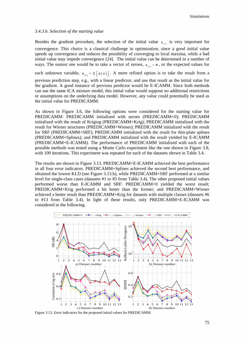
Simulations
75
3.4.3.b. Selection of the starting value
Besides the gradient procedure, the selection of the initial value 0
z is very important for
convergence. This choice is a classical challenge in optimization, since a good initial value
speeds up convergence and reduces the possibility of converging to local maxima, while a bad
initial value may impede convergence [24]. The initial value can be determined in a number of
ways. The easiest one would be to take a vector of zeroes, 0
z 0 , or the expected values for
each unknown variable,
0
E n
z z . A more refined option is to take the result from a
previous prediction step, e.g., with a linear predictor, and use that result as the initial value for
the gradient. A good instance of previous predictor would be E-ICAMM. Since both methods
can use the same ICA mixture model, this initial value would suppose no additional restrictions
or assumptions on the underlying data model. However, any value could potentially be used as
the initial value for PREDICAMM.
As shown in Figure 3.6, the following options were considered for the starting value for
PREDICAMM: PREDICAMM initialized with zeroes (PREDICAMM+0); PREDICAMM
initialized with the result of Kriging (PREDICAMM+Krig); PREDICAMM initialized with the
result for Wiener structures (PREDICAMM+Wiener); PREDICAMM initialized with the result
for SRF (PREDICAMM+SRF); PREDICAMM initialized with the result for thin-plate splines
(PREDICAMM+Splines); and PREDICAMM initialized with the result yielded by E-ICAMM
(PREDICAMM+E-ICAMM). The performance of PREDICAMM initialized with each of the
possible methods was tested using a Monte Carlo experiment like the one shown in Figure 3.8,
with 100 iterations. This experiment was repeated for each of the datasets shown in Table 3.4.
The results are shown in Figure 3.13. PREDICAMM+E-ICAMM achieved the best performance
in all four error indicators. PREDICAMM+Splines achieved the second best performance, and
obtained the lowest KLD (see Figure 3.13.b), while PREDICAMM+SRF performed at a similar
level for single-class cases (datasets #1 to #5 from Table 3.4). The other proposed initial values
performed worse than E-ICAMM and SRF: PREDICAMM+0 yielded the worst result;
PREDICAMM+Krig performed a bit better than the former; and PREDICAMM+Wiener
achieved a better result than PREDICAMM+Krig for datasets with multiple classes (datasets #6
to #13 from Table 3.4). In light of these results, only PREDICAMM+E-ICAMM was
considered in the following.
Figure 3.13. Error indicators for the proposed initial values for PREDICAMM.
1 2 3 4 5 6 7 8 9 10 11 12 13
0
2
4
6
8
a) Dataset number
SIR
(dB
)
1 2 3 4 5 6 7 8 9 10 11 12 13
101
102
b) Dataset number
Kul
lbac
k-L
eibl
er D
iver
genc
e
1 2 3 4 5 6 7 8 9 10 11 12 13
0.2
0.4
0.6
c) Dataset number
Cor
rela
tion
at l
ag z
ero
1 2 3 4 5 6 7 8 9 10 11 12 13
0.2
0.4
0.6
d) Dataset number
MSS
IM
PREDICAMM+0 ...+Krig ...+Splines ...+Wiener ...+SRF ...+E-ICAMM
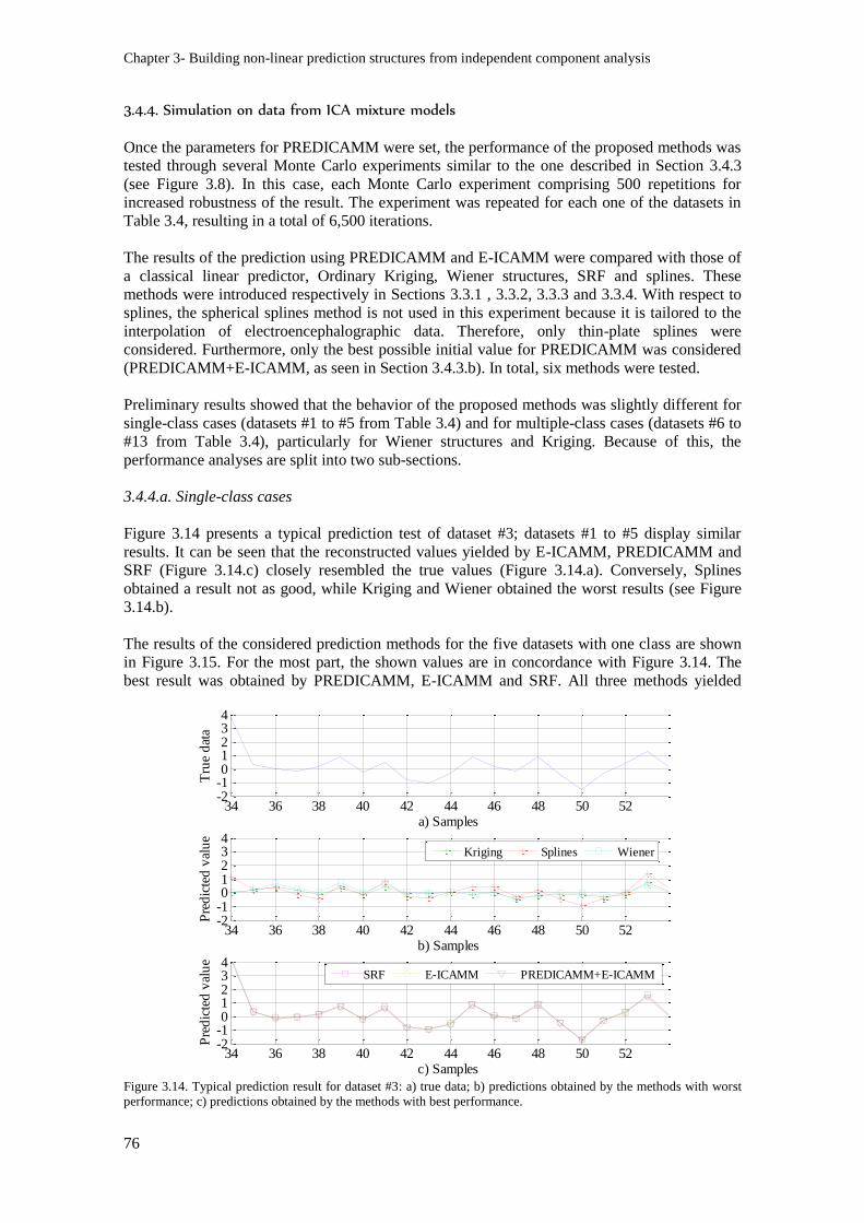
Chapter 3- Building non-linear prediction structures from independent component analysis
76
3.4.4. Simulation on data from ICA mixture models
Once the parameters for PREDICAMM were set, the performance of the proposed methods was
tested through several Monte Carlo experiments similar to the one described in Section 3.4.3
(see Figure 3.8). In this case, each Monte Carlo experiment comprising 500 repetitions for
increased robustness of the result. The experiment was repeated for each one of the datasets in
Table 3.4, resulting in a total of 6,500 iterations.
The results of the prediction using PREDICAMM and E-ICAMM were compared with those of
a classical linear predictor, Ordinary Kriging, Wiener structures, SRF and splines. These
methods were introduced respectively in Sections 3.3.1 , 3.3.2, 3.3.3 and 3.3.4. With respect to
splines, the spherical splines method is not used in this experiment because it is tailored to the
interpolation of electroencephalographic data. Therefore, only thin-plate splines were
considered. Furthermore, only the best possible initial value for PREDICAMM was considered
(PREDICAMM+E-ICAMM, as seen in Section 3.4.3.b). In total, six methods were tested.
Preliminary results showed that the behavior of the proposed methods was slightly different for
single-class cases (datasets #1 to #5 from Table 3.4) and for multiple-class cases (datasets #6 to
#13 from Table 3.4), particularly for Wiener structures and Kriging. Because of this, the
performance analyses are split into two sub-sections.
3.4.4.a. Single-class cases
Figure 3.14 presents a typical prediction test of dataset #3; datasets #1 to #5 display similar
results. It can be seen that the reconstructed values yielded by E-ICAMM, PREDICAMM and
SRF (Figure 3.14.c) closely resembled the true values (Figure 3.14.a). Conversely, Splines
obtained a result not as good, while Kriging and Wiener obtained the worst results (see Figure
3.14.b).
The results of the considered prediction methods for the five datasets with one class are shown
in Figure 3.15. For the most part, the shown values are in concordance with Figure 3.14. The
best result was obtained by PREDICAMM, E-ICAMM and SRF. All three methods yielded
Figure 3.14. Typical prediction result for dataset #3: a) true data; b) predictions obtained by the methods with worst
performance; c) predictions obtained by the methods with best performance.
34 36 38 40 42 44 46 48 50 52-2-101234
a) Samples
Tru
e d
ata
34 36 38 40 42 44 46 48 50 52-2-101234
b) Samples
Pre
dic
ted
val
ue
34 36 38 40 42 44 46 48 50 52-2-101234
c) Samples
Pre
dic
ted
val
ue
Kriging Splines Wiener
SRF E-ICAMM PREDICAMM+E-ICAMM
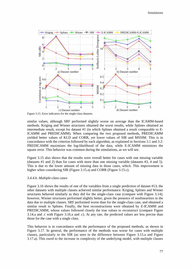
Simulations
77
Figure 3.15. Error indicators for the single-class datasets.
similar values, although SRF performed slightly worse on average than the ICAMM-based
methods. Kriging and Wiener structures obtained the worst results, while Splines obtained an
intermediate result, except for dataset #1 (in which Splines obtained a result comparable to E-
ICAMM and PREDICAMM). When comparing the two proposed methods, PREDICAMM
yielded better values of KLD and CORR, yet lower values of SIR and MSSIM. This is in
concordance with the criterion followed by each algorithm, as explained in Sections 3.1 and 3.2:
PREDICAMM maximizes the log-likelihood of the data, while E-ICAMM minimizes the
square error. This behavior was common during the simulations, as we will see.
Figure 3.15 also shows that the results were overall better for cases with one missing variable
(datasets #1 and 2) than for cases with more than one missing variable (datasets #3, 4 and 5).
This is due to the lower amount of missing data in those cases, which. This improvement is
higher when considering SIR (Figure 3.15.a) and CORR (Figure 3.15.c).
3.4.4.b. Multiple-class cases
Figure 3.16 shows the results of one of the variables from a single prediction of dataset #13; the
other datasets with multiple classes achieved similar performance. Kriging, Splines and Wiener
structures behaved similarly as they did for the single-class case (compare with Figure 3.14);
however, Wiener structures performed slightly better, given the presence of nonlinearities in the
data due to multiple classes. SRF performed worse than for the single-class case, and obtained a
similar result to Splines. Finally, the best reconstructions were obtained by E-ICAMM and
PREDICAMM, whose values followed closely the true values to reconstruct (compare Figure
3.14.a and .c with Figure 3.16.a and .c). At any rate, the predicted values are less precise than
those for the case with a single class.
This behavior is in concordance with the performance of the proposed methods, as shown in
Figure 3.17. In general, the performance of the methods was worse for cases with multiple
classes, particularly in the SIR (as seen in the difference between Figure 3.15.a and Figure
3.17.a). This owed to the increase in complexity of the underlying model, with multiple classes
1 2 3 4 50
2
4
6
8
a) Dataset number
SIR
(d
B)
1 2 3 4 5
102
b) Dataset number
Ku
llb
ack
-Leib
ler
Div
erg
en
ce
1 2 3 4 5
0.2
0.4
0.6
c) Dataset number
Co
rrela
tio
n a
t la
g z
ero
1 2 3 4 5
0.1
0.2
0.3
0.4
0.5
d) Dataset number
MS
SIM
Kriging Splines Wiener SRF E-ICAMM PREDICAMM+E-ICAMM
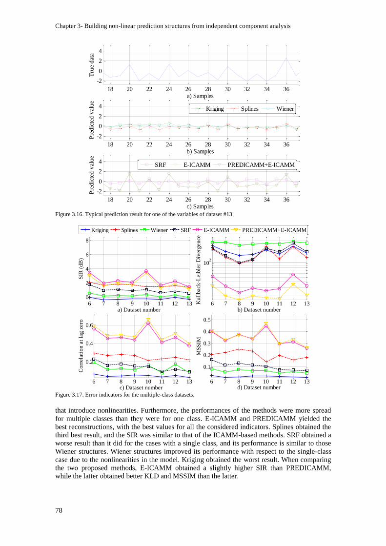
Chapter 3- Building non-linear prediction structures from independent component analysis
78
Figure 3.16. Typical prediction result for one of the variables of dataset #13.
Figure 3.17. Error indicators for the multiple-class datasets.
that introduce nonlinearities. Furthermore, the performances of the methods were more spread
for multiple classes than they were for one class. E-ICAMM and PREDICAMM yielded the
best reconstructions, with the best values for all the considered indicators. Splines obtained the
third best result, and the SIR was similar to that of the ICAMM-based methods. SRF obtained a
worse result than it did for the cases with a single class, and its performance is similar to those
Wiener structures. Wiener structures improved its performance with respect to the single-class
case due to the nonlinearities in the model. Kriging obtained the worst result. When comparing
the two proposed methods, E-ICAMM obtained a slightly higher SIR than PREDICAMM,
while the latter obtained better KLD and MSSIM than the latter.
18 20 22 24 26 28 30 32 34 36
-2
0
2
4
a) SamplesT
rue
dat
a
18 20 22 24 26 28 30 32 34 36
-2
0
2
4
b) Samples
Pre
dic
ted
val
ue
18 20 22 24 26 28 30 32 34 36
-2
0
2
4
c) Samples
Pre
dic
ted
val
ue
Kriging Splines Wiener
SRF E-ICAMM PREDICAMM+E-ICAMM
6 7 8 9 10 11 12 130
2
4
6
8
a) Dataset number
SIR
(d
B)
6 7 8 9 10 11 12 13
102
b) Dataset number
Ku
llb
ack
-Leib
ler
Div
erg
en
ce
6 7 8 9 10 11 12 13
0.2
0.4
0.6
c) Dataset number
Co
rrela
tio
n a
t la
g z
ero
6 7 8 9 10 11 12 13
0.1
0.2
0.3
0.4
0.5
d) Dataset number
MS
SIM
Kriging Splines Wiener SRF E-ICAMM PREDICAMM+E-ICAMM
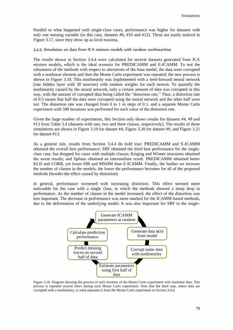
Simulations
79
Parallel to what happened with single-class cases, performance was higher for datasets with
only one missing variable (in this case, datasets #6, #10 and #12). These are easily noticed in
Figure 3.17, since they show up as local maxima.
3.4.5. Simulation on data from ICA mixture models with random nonlinearities
The results shown in Section 3.4.4 were calculated for several datasets generated from ICA
mixture models, which is the ideal scenario for PREDICAMM and E-ICAMM. To test the
robustness of the methods with respect to alterations of the base model, the data were corrupted
with a nonlinear element and then the Monte Carlo experiment was repeated; the new process is
shown in Figure 3.18. This nonlinearity was implemented with a feed-forward neural network
(one hidden layer with 30 neurons) with random weights for each neuron. To quantify the
nonlinearity caused by the neural network, only a certain amount of data was corrupted in this
way, with the amount of corrupted data being called the “distortion rate.” Thus, a distortion rate
of 0.5 means that half the data were corrupted using the neural network and the other half were
not. The distortion rate was changed from 0 to 1 in steps of 0.1, and a separate Monte Carlo
experiment with 500 iterations was performed for each value of the distortion rate.
Given the large number of experiments, this Section only shows results for datasets #4, #9 and
#13 from Table 3.4 (datasets with one, two and three classes, respectively). The results of these
simulations are shown in Figure 3.19 for dataset #4, Figure 3.20 for dataset #9, and Figure 3.21
for dataset #13.
As a general rule, results from Section 3.4.4 do hold true: PREDICAMM and E-ICAMM
obtained the overall best performance; SRF obtained the third best performance for the single-
class case, but dropped for cases with multiple classes; Kriging and Wiener structures obtained
the worst results; and Splines obtained an intermediate result. PREDICAMM obtained better
KLD and CORR, yet lower SIR and MSSIM than E-ICAMM. Finally, the further we increase
the number of classes in the models, the lower the performance becomes for all of the proposed
methods (besides the effect caused by distortion).
In general, performance worsened with increasing distortion. This effect seemed more
noticeable for the case with a single class, in which the methods showed a steep drop in
performance. As the number of classes in the model increased, the effect of the distortion was
less important. The decrease in performance was more marked for the ICAMM-based methods,
due to the deformation of the underlying model. It was also important for SRF in the single-
Figure 3.18. Diagram showing the process of each iteration of the Monte Carlo experiment with nonlinear data. This
process is repeated several times during each Monte Carlo experiment. Note that the third step, where data are
corrupted with a nonlinearity, is what separates it from the Monte Carlo experiment in Section 3.4.4.
Generate ICAMM parameters at random
Generate data x(n) from model
Corrupt some data with nonlinearity
Estimate parameters using first half of
data
Predict missing traces on second
half of data
Calculate prediction performance
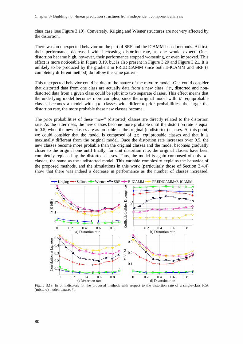
Chapter 3- Building non-linear prediction structures from independent component analysis
80
class case (see Figure 3.19). Conversely, Kriging and Wiener structures are not very affected by
the distortion.
There was an unexpected behavior on the part of SRF and the ICAMM-based methods. At first,
their performance decreased with increasing distortion rate, as one would expect. Once
distortion became high, however, their performance stopped worsening, or even improved. This
effect is more noticeable in Figure 3.19, but is also present in Figure 3.20 and Figure 3.21. It is
unlikely to be produced by the gradient in PREDICAMM since both E-ICAMM and SRF (a
completely different method) do follow the same pattern.
This unexpected behavior could be due to the nature of the mixture model. One could consider
that distorted data from one class are actually data from a new class, i.e., distorted and non-
distorted data from a given class could be split into two separate classes. This effect means that
the underlying model becomes more complex, since the original model with K equiprobable
classes becomes a model with 2 K classes with different prior probabilities; the larger the
distortion rate, the more probable these new classes become.
The prior probabilities of these “new” (distorted) classes are directly related to the distortion
rate. As the latter rises, the new classes become more probable until the distortion rate is equal
to 0.5, when the new classes are as probable as the original (undistorted) classes. At this point,
we could consider that the model is composed of 2 K equiprobable classes and that it is
maximally different from the original model. Once the distortion rate increases over 0.5, the
new classes become more probable than the original classes and the model becomes gradually
closer to the original one until finally, for unit distortion rate, the original classes have been
completely replaced by the distorted classes. Thus, the model is again composed of only K
classes, the same as the undistorted model. This variable complexity explains the behavior of
the proposed methods, and the simulations in this work (particularly those of Section 3.4.4)
show that there was indeed a decrease in performance as the number of classes increased.
Figure 3.19. Error indicators for the proposed methods with respect to the distortion rate of a single-class ICA
(mixture) model, dataset #4.
0 0.2 0.4 0.6 0.8
0
1
2
3
a) Distortion rate
SIR
(dB
)
0 0.2 0.4 0.6 0.8
102
b) Distortion rate
Kull
back-L
eib
ler
Div
erg
ence
0 0.2 0.4 0.6 0.8
0.1
0.2
0.3
0.4
0.5
c) Distortion rate
Corr
ela
tion a
t la
g z
ero
0 0.2 0.4 0.6 0.8
0.1
0.2
0.3
d) Distortion rate
MS
SIM
Kriging Splines Wiener SRF E-ICAMM PREDICAMM+E-ICAMM
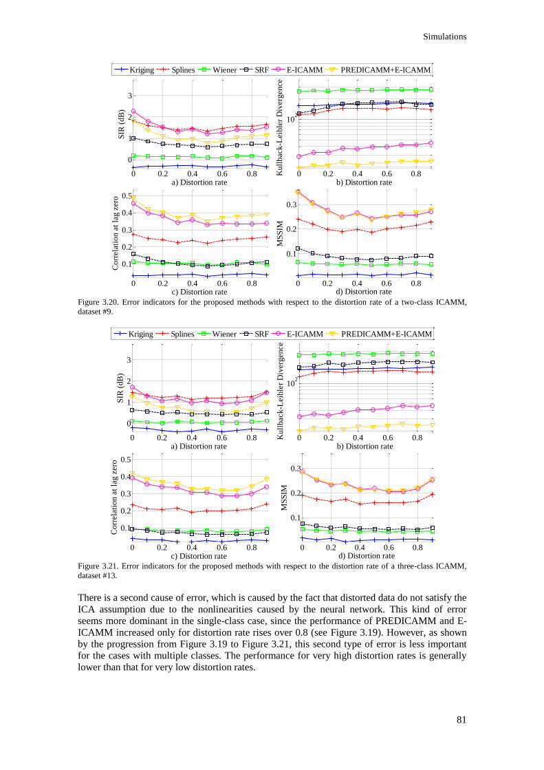
Simulations
81
Figure 3.20. Error indicators for the proposed methods with respect to the distortion rate of a two-class ICAMM,
dataset #9.
Figure 3.21. Error indicators for the proposed methods with respect to the distortion rate of a three-class ICAMM,
dataset #13.
There is a second cause of error, which is caused by the fact that distorted data do not satisfy the
ICA assumption due to the nonlinearities caused by the neural network. This kind of error
seems more dominant in the single-class case, since the performance of PREDICAMM and E-
ICAMM increased only for distortion rate rises over 0.8 (see Figure 3.19). However, as shown
by the progression from Figure 3.19 to Figure 3.21, this second type of error is less important
for the cases with multiple classes. The performance for very high distortion rates is generally
lower than that for very low distortion rates.
0 0.2 0.4 0.6 0.8
0
1
2
3
a) Distortion rate
SIR
(dB
)
0 0.2 0.4 0.6 0.8
102
b) Distortion rate
Kull
back-L
eib
ler
Div
erg
ence
0 0.2 0.4 0.6 0.8
0.1
0.2
0.3
0.4
0.5
c) Distortion rate
Corr
ela
tion a
t la
g z
ero
0 0.2 0.4 0.6 0.8
0.1
0.2
0.3
d) Distortion rate
MS
SIM
Kriging Splines Wiener SRF E-ICAMM PREDICAMM+E-ICAMM
0 0.2 0.4 0.6 0.8
0
1
2
3
a) Distortion rate
SIR
(d
B)
0 0.2 0.4 0.6 0.8
102
b) Distortion rate
Ku
llb
ack
-Leib
ler
Div
erg
en
ce
0 0.2 0.4 0.6 0.8
0.1
0.2
0.3
0.4
0.5
c) Distortion rate
Co
rrela
tio
n a
t la
g z
ero
0 0.2 0.4 0.6 0.8
0.1
0.2
0.3
d) Distortion rate
MS
SIM
Kriging Splines Wiener SRF E-ICAMM PREDICAMM+E-ICAMM
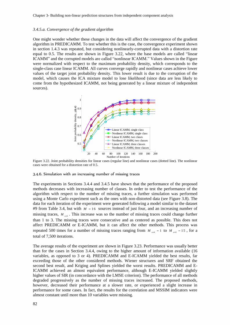
Chapter 3- Building non-linear prediction structures from independent component analysis
82
3.4.5.a. Convergence of the gradient algorithm
One might wonder whether these changes in the data will affect the convergence of the gradient
algorithm in PREDICAMM. To test whether this is the case, the convergence experiment shown
in section 1.4.3 was repeated, but considering nonlinearly-corrupted data with a distortion rate
equal to 0.5. The results are shown in Figure 3.22, where the base models are called “linear
ICAMM” and the corrupted models are called “nonlinear ICAMM.” Values shown in the Figure
were normalized with respect to the maximum probability density, which corresponds to the
single-class case linear ICAMM. All curves converge rapidly and nonlinear cases achieve lower
values of the target joint probability density. This lower result is due to the corruption of the
model, which causes the ICA mixture model to lose likelihood (since data are less likely to
come from the hypothesized ICAMM, not being generated by a linear mixture of independent
sources).
Figure 3.22. Joint probability densities for linear cases (regular line) and nonlinear cases (dotted line). The nonlinear
cases were obtained for a distortion rate of 0.5.
3.4.6. Simulation with an increasing number of missing traces
The experiments in Sections 3.4.4 and 3.4.5 have shown that the performance of the proposed
methods decreases with increasing number of classes. In order to test the performance of the
algorithm with respect to the number of missing traces, a further simulation was performed
using a Monte Carlo experiment such as the ones with non-distorted data (see Figure 3.8). The
data for each iteration of the experiment were generated following a model similar to the dataset
#9 from Table 3.4, but with 16M sources instead of just four, and an increasing number of
missing traces, u n k
M . This increase was so the number of missing traces could change further
than 1 to 3. The missing traces were consecutive and as centered as possible. This does not
affect PREDICAMM or E-ICAMM, but it can affect the other methods. This process was
repeated 500 times for a number of missing traces ranging from 1u n k
M to 1 5u n k
M , for a
total of 7,500 iterations.
The average results of the experiment are shown in Figure 3.23. Performance was usually better
than for the cases in Section 3.4.4, owing to the higher amount of information available (16
variables, as opposed to 3 or 4). PREDICAMM and E-ICAMM yielded the best results, far
exceeding those of the other considered methods. Wiener structures and SRF obtained the
second best result, and Kriging and Splines yielded the worst results. PREDICAMM and E-
ICAMM achieved an almost equivalent performance, although E-ICAMM yielded slightly
higher values of SIR (in concordance with the LMSE criterion). The performance of all methods
degraded progressively as the number of missing traces increased. The proposed methods,
however, decreased their performance at a slower rate, or experienced a slight increase in
performance for some cases. In fact, the results for the correlation and MSSIM indicators were
almost constant until more than 10 variables were missing.
20 40 60 80 100 120 140 160 180 200
0.5
0.6
0.7
0.8
0.9
1
Number of iterations
Join
t p
rob
abil
ity
den
sity
, p
( y,z
)
Linear ICAMM, single class
Nonlinear ICAMM, single class
Linear ICAMM, two clases
Nonlinear ICAMM, two classes
Linear ICAMM, three classes
Nonlinear ICAMM, three classes
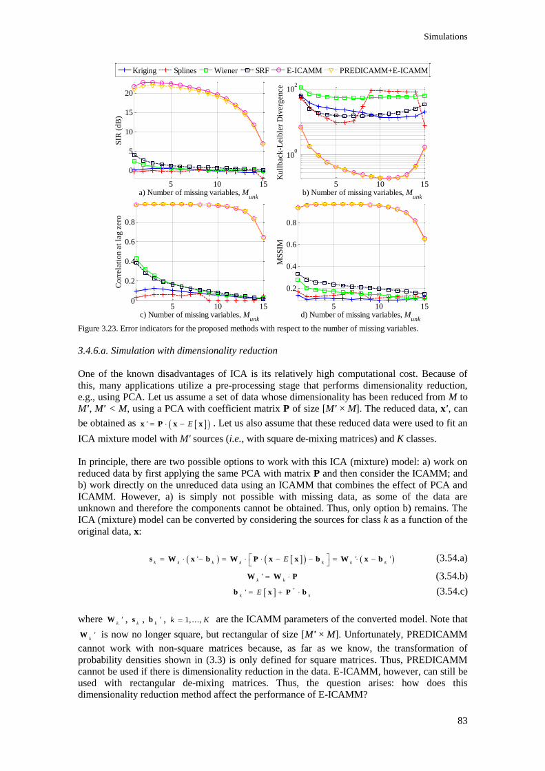
Simulations
83
Figure 3.23. Error indicators for the proposed methods with respect to the number of missing variables.
3.4.6.a. Simulation with dimensionality reduction
One of the known disadvantages of ICA is its relatively high computational cost. Because of
this, many applications utilize a pre-processing stage that performs dimensionality reduction,
e.g., using PCA. Let us assume a set of data whose dimensionality has been reduced from M to
M', M' < M, using a PCA with coefficient matrix P of size [M' × M]. The reduced data, x', can
be obtained as ' E x P x x . Let us also assume that these reduced data were used to fit an
ICA mixture model with M' sources (i.e., with square de-mixing matrices) and K classes.
In principle, there are two possible options to work with this ICA (mixture) model: a) work on
reduced data by first applying the same PCA with matrix P and then consider the ICAMM; and
b) work directly on the unreduced data using an ICAMM that combines the effect of PCA and
ICAMM. However, a) is simply not possible with missing data, as some of the data are
unknown and therefore the components cannot be obtained. Thus, only option b) remains. The
ICA (mixture) model can be converted by considering the sources for class k as a function of the
original data, x:
' ' 'k k k k k k k
E
s W x b W P x x b W x b (3.54.a)
'k k
W W P (3.54.b)
'k k
E
b x P b (3.54.c)
where 'k
W , k
s , 'k
b , 1, ...,k K are the ICAMM parameters of the converted model. Note that
'k
W is now no longer square, but rectangular of size [M' × M]. Unfortunately, PREDICAMM
cannot work with non-square matrices because, as far as we know, the transformation of
probability densities shown in (3.3) is only defined for square matrices. Thus, PREDICAMM
cannot be used if there is dimensionality reduction in the data. E-ICAMM, however, can still be
used with rectangular de-mixing matrices. Thus, the question arises: how does this
dimensionality reduction method affect the performance of E-ICAMM?
5 10 15
0
5
10
15
20
a) Number of missing variables, Munk
SIR
(d
B)
5 10 15
100
102
b) Number of missing variables, Munk
Ku
llb
ack
-Leib
ler
Div
erg
en
ce
5 10 150
0.2
0.4
0.6
0.8
c) Number of missing variables, Munk
Co
rrela
tio
n a
t la
g z
ero
5 10 15
0.2
0.4
0.6
0.8
d) Number of missing variables, Munk
MS
SIM
Kriging Splines Wiener SRF E-ICAMM PREDICAMM+E-ICAMM
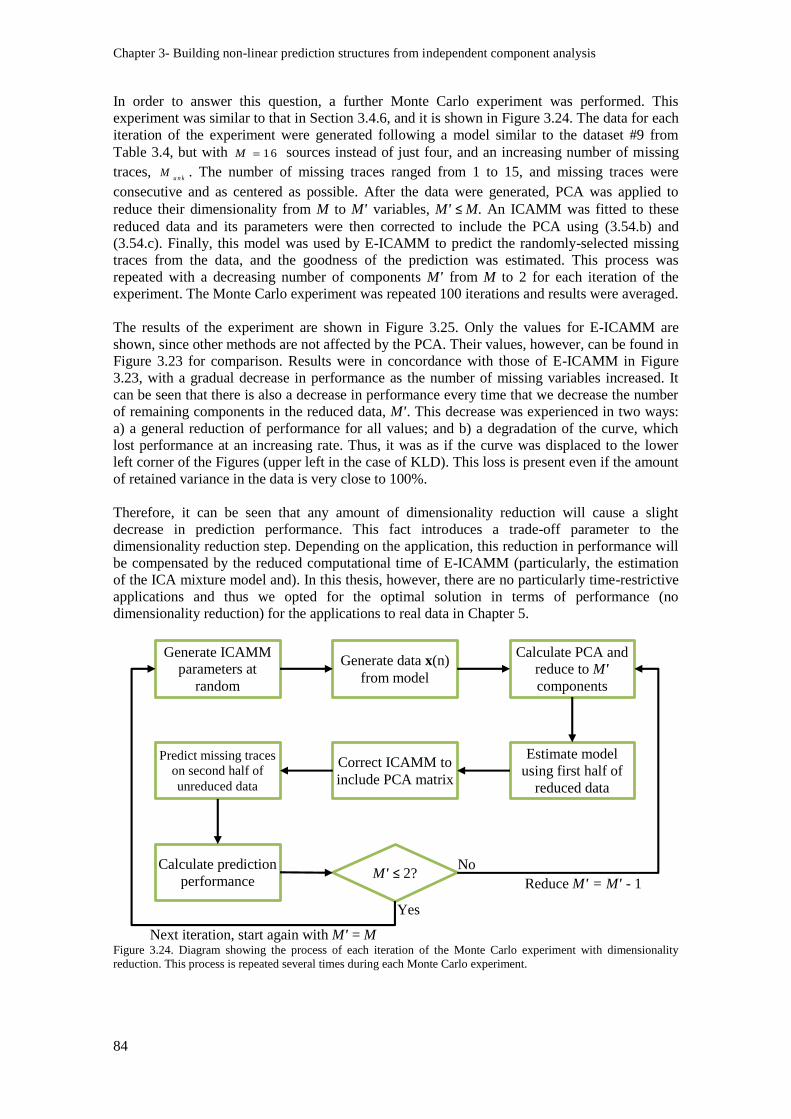
Chapter 3- Building non-linear prediction structures from independent component analysis
84
In order to answer this question, a further Monte Carlo experiment was performed. This
experiment was similar to that in Section 3.4.6, and it is shown in Figure 3.24. The data for each
iteration of the experiment were generated following a model similar to the dataset #9 from
Table 3.4, but with 16M sources instead of just four, and an increasing number of missing
traces, u n k
M . The number of missing traces ranged from 1 to 15, and missing traces were
consecutive and as centered as possible. After the data were generated, PCA was applied to
reduce their dimensionality from M to M' variables, M' ≤ M. An ICAMM was fitted to these
reduced data and its parameters were then corrected to include the PCA using (3.54.b) and
(3.54.c). Finally, this model was used by E-ICAMM to predict the randomly-selected missing
traces from the data, and the goodness of the prediction was estimated. This process was
repeated with a decreasing number of components M' from M to 2 for each iteration of the
experiment. The Monte Carlo experiment was repeated 100 iterations and results were averaged.
The results of the experiment are shown in Figure 3.25. Only the values for E-ICAMM are
shown, since other methods are not affected by the PCA. Their values, however, can be found in
Figure 3.23 for comparison. Results were in concordance with those of E-ICAMM in Figure
3.23, with a gradual decrease in performance as the number of missing variables increased. It
can be seen that there is also a decrease in performance every time that we decrease the number
of remaining components in the reduced data, M'. This decrease was experienced in two ways:
a) a general reduction of performance for all values; and b) a degradation of the curve, which
lost performance at an increasing rate. Thus, it was as if the curve was displaced to the lower
left corner of the Figures (upper left in the case of KLD). This loss is present even if the amount
of retained variance in the data is very close to 100%.
Therefore, it can be seen that any amount of dimensionality reduction will cause a slight
decrease in prediction performance. This fact introduces a trade-off parameter to the
dimensionality reduction step. Depending on the application, this reduction in performance will
be compensated by the reduced computational time of E-ICAMM (particularly, the estimation
of the ICA mixture model and). In this thesis, however, there are no particularly time-restrictive
applications and thus we opted for the optimal solution in terms of performance (no
dimensionality reduction) for the applications to real data in Chapter 5.
Figure 3.24. Diagram showing the process of each iteration of the Monte Carlo experiment with dimensionality
reduction. This process is repeated several times during each Monte Carlo experiment.
Generate ICAMM
parameters at
random
Generate data x(n)
from model
Calculate PCA and
reduce to M'
components
Estimate model
using first half of
reduced data
Correct ICAMM to
include PCA matrix
Predict missing traces
on second half of
unreduced data
Calculate prediction
performance M' ≤ 2?
No
Yes
Next iteration, start again with M' = M
Reduce M' = M' - 1
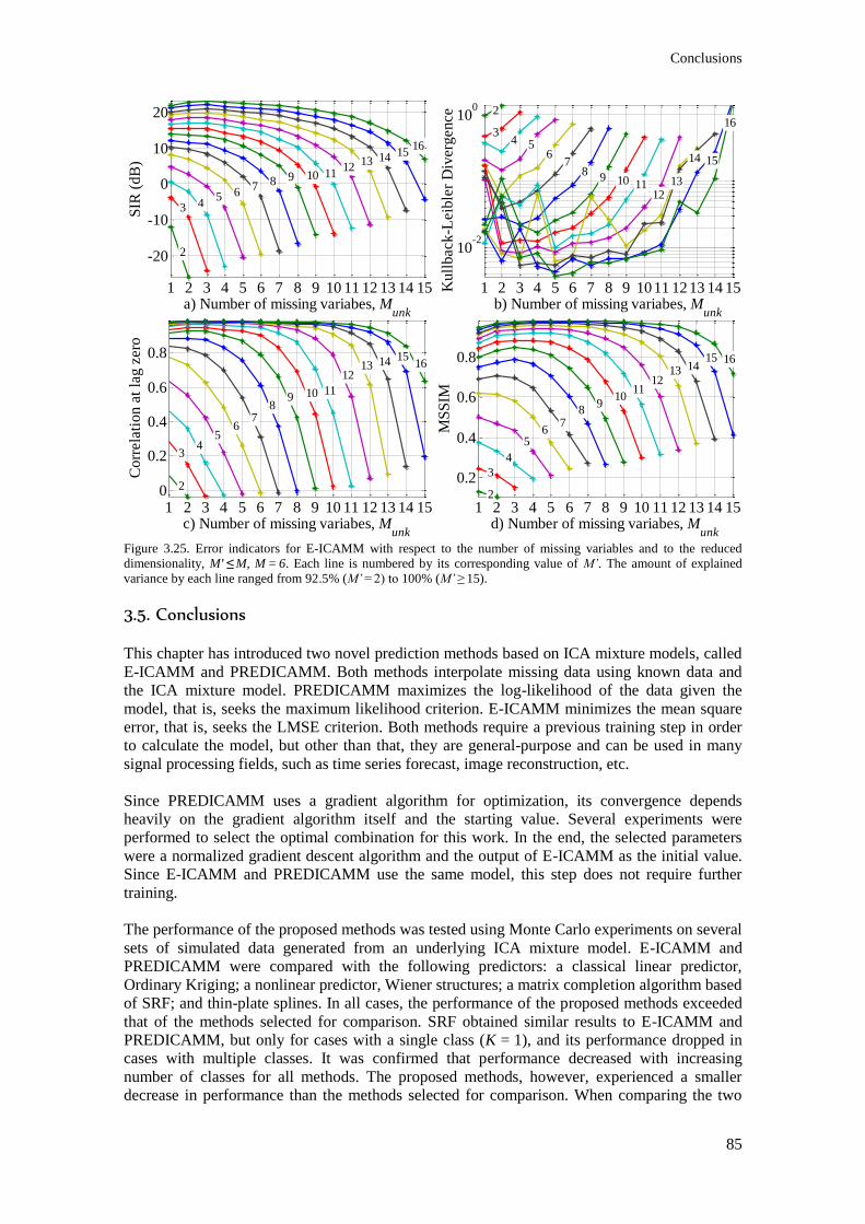
Conclusions
85
Figure 3.25. Error indicators for E-ICAMM with respect to the number of missing variables and to the reduced
dimensionality, M' ≤ M, M = 6. Each line is numbered by its corresponding value of M’. The amount of explained
variance by each line ranged from 92.5% (M’ = 2) to 100% (M’ ≥ 15).
3.5. Conclusions
This chapter has introduced two novel prediction methods based on ICA mixture models, called
E-ICAMM and PREDICAMM. Both methods interpolate missing data using known data and
the ICA mixture model. PREDICAMM maximizes the log-likelihood of the data given the
model, that is, seeks the maximum likelihood criterion. E-ICAMM minimizes the mean square
error, that is, seeks the LMSE criterion. Both methods require a previous training step in order
to calculate the model, but other than that, they are general-purpose and can be used in many
signal processing fields, such as time series forecast, image reconstruction, etc.
Since PREDICAMM uses a gradient algorithm for optimization, its convergence depends
heavily on the gradient algorithm itself and the starting value. Several experiments were
performed to select the optimal combination for this work. In the end, the selected parameters
were a normalized gradient descent algorithm and the output of E-ICAMM as the initial value.
Since E-ICAMM and PREDICAMM use the same model, this step does not require further
training.
The performance of the proposed methods was tested using Monte Carlo experiments on several
sets of simulated data generated from an underlying ICA mixture model. E-ICAMM and
PREDICAMM were compared with the following predictors: a classical linear predictor,
Ordinary Kriging; a nonlinear predictor, Wiener structures; a matrix completion algorithm based
of SRF; and thin-plate splines. In all cases, the performance of the proposed methods exceeded
that of the methods selected for comparison. SRF obtained similar results to E-ICAMM and
PREDICAMM, but only for cases with a single class (K = 1), and its performance dropped in
cases with multiple classes. It was confirmed that performance decreased with increasing
number of classes for all methods. The proposed methods, however, experienced a smaller
decrease in performance than the methods selected for comparison. When comparing the two
1 2 3 4 5 6 7 8 9 10 11 12 13 14 15
-20
-10
0
10
20
a) Number of missing variabes, Munk
SIR
(d
B)
2
3 45 6
7 8 9 10 1112
13 14 1516
1 2 3 4 5 6 7 8 9 1011 12 13 14 15
10-2
100
b) Number of missing variabes, Munk
Ku
llb
ack
-Leib
ler
Div
erg
en
ce 2
34 5
67
89 10 11
1213
14 15
16
1 2 3 4 5 6 7 8 9 10 11 12 13 14 150
0.2
0.4
0.6
0.8
c) Number of missing variabes, Munk
Co
rrela
tio
n a
t la
g z
ero
2
34
56
78
9 10 11
1213 14 15
16
1 2 3 4 5 6 7 8 9 10 11 12 13 14 15
0.2
0.4
0.6
0.8
d) Number of missing variabes, Munk
MS
SIM
2
3
4
56
78
910
1112
13 1415 16

Chapter 3- Building non-linear prediction structures from independent component analysis
86
proposed methods with one another, PREDICAMM obtained better values of CORR and KLD,
while E-ICAMM obtained better values of SIR and MSSIM. Their performances, however,
were similar.
A second set of Monte Carlo experiments was run to test the behavior of the proposed methods
with respect to alterations of the underlying model. To this effect, the performance was run with
data generated from an ICAMM and then corrupted by a nonlinear element. This nonlinearity
was implemented by a randomly-initialized neural network. Results for this second series of
tests were similar to those for the first series, and E-ICAMM and PREDICAMM obtained the
best performance even though the base model was not completely valid. All considered methods
decreased their performance as the number of distorted data grew larger. The proposed
ICAMM-based methods and SRF were the most affected by this effect, while Kriging, Wiener
structures and Splines were the least affected. It was shown that this decrease in performance
owed to the increase in complexity in the underlying model (i.e., the distorted data were treated
as new “classes” of data), rather than to the distortion of the validity of the ICA mixture model.
Another Monte Carlo experiment was run to test the performance of E-ICAMM and
PREDICAMM with respect to the number of missing data, u n k
M . The results of this experiment
were consistent with those of the previous experiments, and the proposed methods obtained the
best performance. Both proposed methods yielded very similar results, although E-ICAMM
obtained slightly better SIR values. All methods decreased in performance as the number of
missing data increased, and this decrease was much slower for the proposed methods.
PREDICAMM and E-ICAMM achieved a good performance until the number of missing traces
was high ( 1 0u n k
M out of 16 variables). This demonstrates the robustness of E-ICAMM and
PREDICAMM with respect to the number of missing data.
A final Monte Carlo experiment tested the performance of the proposed methods when
dimensionality reduction is performed before estimating the underlying ICAMM. Since
PREDICAMM cannot function in this case, only E-ICAMM was considered for this final test.
The experiments confirm the loss in performance with increasing number of missing values.
Furthermore, the dimensionality reduction method did cause a further decrease in performance.
This loss is present even if the amount of retained variance in the data is very close to 100%.
Therefore, the dimensionality reduction method introduces a trade-off between performance and
computational time.
87
A general dynamic modeling approach based on synchronized ICA mixture models: G- and UG-SICAMM
4


89
- A general dynamic modeling approach based on synchronized ICA mixture models: G- and UG-SICAMM
This chapter presents two new procedures for dynamic modeling which are based on
synchronized ICA mixture models. The starting point of this work is a method that incorporates
a hidden Markov model to extend the ICA mixture models to the case of having sequential
dependence in the feature observation records. This method can be used to model the dynamic
changes of a process in time; we called it sequential ICAMM (SICAMM) [230]. The proposed
methods in this chapter extend the one Markov chain employed featured in SICAMM to a
general framework to characterize the joint behavior of a number of synchronized dynamic
models or “chains.” We have called these methods Generalized Sequential ICAMM (G-
SICAMM) and UG-SICAMM (Unsupervised G-SICAMM). This latter maximizes the log-
likelihood of the model with respect to all of the available training data and the parameters of
the model. It could be named SG-SICAMM because it also considers the semi-supervised case.
The procedures can be used for classification using maximum a posteriori estimation and the
forward-backward procedures as in Baum-Welch and Viterbi algorithms [17,270]. Thus, we
have tested the classification accuracy and goodness of fit of G-SICAMM and UG-SICAMM
using several sets of synthetic data with two chains and two, three and four classes per chain.
Furthermore, the behavior of the proposed methods with respect to dynamically-changing
sources is studied. G-SICAMM is compared with dynamic Bayesian networks (DBN), a state-
of-the-art method for dynamic modeling. The comparison shows that the proposed method
performs better than DBN, even if the sources change dynamically, and thus, the adaptive
capabilities of the method to non-stationary process are demonstrated. In addition, we found that
the G-SICAMM parameters can be studied to gain further understanding of the modeled data,
whereas the DBN parameters cannot be examined in this way.
Let us consider this latter point for a moment. Most of the applications of the proposed method
revolve around classification of data in several categories, i.e., the result is a discrete value. In
addition, most of the classification methods (e.g., discriminant analysis, DA [169], and Naïve
Bayes, [175]) only perform classification and their parameters are difficult to interpret or shed
no further light on the classified data. However, there are methods which obtain not only a
classification of the data, but also a structured result which is, by itself, a way to interpret the
data. Two instances of this kind of methods are decision tree learning [206] and hierarchical
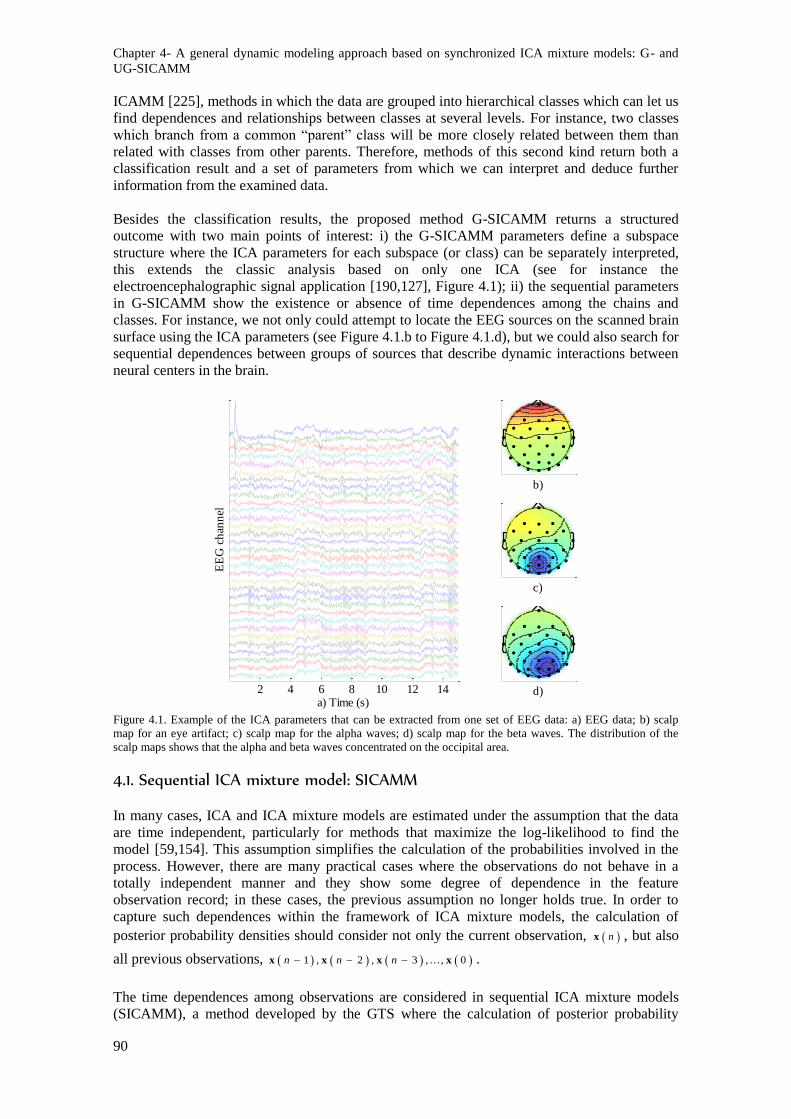
Chapter 4- A general dynamic modeling approach based on synchronized ICA mixture models: G- and
UG-SICAMM
90
ICAMM [225], methods in which the data are grouped into hierarchical classes which can let us
find dependences and relationships between classes at several levels. For instance, two classes
which branch from a common “parent” class will be more closely related between them than
related with classes from other parents. Therefore, methods of this second kind return both a
classification result and a set of parameters from which we can interpret and deduce further
information from the examined data.
Besides the classification results, the proposed method G-SICAMM returns a structured
outcome with two main points of interest: i) the G-SICAMM parameters define a subspace
structure where the ICA parameters for each subspace (or class) can be separately interpreted,
this extends the classic analysis based on only one ICA (see for instance the
electroencephalographic signal application [190,127], Figure 4.1); ii) the sequential parameters
in G-SICAMM show the existence or absence of time dependences among the chains and
classes. For instance, we not only could attempt to locate the EEG sources on the scanned brain
surface using the ICA parameters (see Figure 4.1.b to Figure 4.1.d), but we could also search for
sequential dependences between groups of sources that describe dynamic interactions between
neural centers in the brain.
Figure 4.1. Example of the ICA parameters that can be extracted from one set of EEG data: a) EEG data; b) scalp
map for an eye artifact; c) scalp map for the alpha waves; d) scalp map for the beta waves. The distribution of the
scalp maps shows that the alpha and beta waves concentrated on the occipital area.
4.1. Sequential ICA mixture model: SICAMM
In many cases, ICA and ICA mixture models are estimated under the assumption that the data
are time independent, particularly for methods that maximize the log-likelihood to find the
model [59,154]. This assumption simplifies the calculation of the probabilities involved in the
process. However, there are many practical cases where the observations do not behave in a
totally independent manner and they show some degree of dependence in the feature
observation record; in these cases, the previous assumption no longer holds true. In order to
capture such dependences within the framework of ICA mixture models, the calculation of
posterior probability densities should consider not only the current observation, nx , but also
all previous observations, 1 , 2 , 3 , ... , 0n n n x x x x .
The time dependences among observations are considered in sequential ICA mixture models
(SICAMM), a method developed by the GTS where the calculation of posterior probability
2 4 6 8 10 12 14a) Time (s)
EE
G c
han
nel
b)
c)
d)
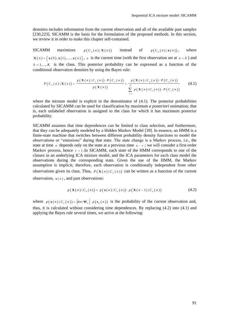
Sequential ICA mixture model: SICAMM
91
densities includes information from the current observation and all of the available past samples
[230,223]. SICAMM is the basis for the formulation of the proposed methods. In this section,
we review it in order to make this chapter self-contained.
SICAMM maximizes |k
p C n nX instead of |k
p C n nx , where
0 , 1 , ....,n n
X x x x , n is the current time (with the first observation set at 0n ) and
1, ...,k K is the class. This posterior probability can be expressed as a function of the
conditional observation densities by using the Bayes rule:
1
| ||
|
k k k k
k K
l l
l
p n C n P C n p n C n P C nP C n n
p np n C n P C n
X XX
XX
(4.1)
where the mixture model is explicit in the denominator of (4.1). The posterior probabilities
calculated by SICAMM can be used for classification by maximum a posteriori estimation; that
is, each unlabeled observation is assigned to the class for which it has maximum posterior
probability.
SICAMM assumes that time dependences can be limited to class selection, and furthermore,
that they can be adequately modeled by a Hidden Markov Model [39]. In essence, an HMM is a
finite-state machine that switches between different probability density functions to model the
observations or “emissions” during that state. The state change is a Markov process, i.e., the
state at time n depends only on the state at a previous time n ; we will consider a first-order
Markov process, hence 1 .In SICAMM, each state of the HMM corresponds to one of the
classes in an underlying ICA mixture model, and the ICA parameters for each class model the
observations during the corresponding state. Given the use of the HMM, the Markov
assumption is implicit; therefore, each observation is conditionally independent from other
observations given its class. Thus, |k
P n C nX can be written as a function of the current
observation, nx , and past observations:
| | 1 |k k k
p n C n p n C n p n C n X x X (4.2)
where | detk k k
p n C n p n x W s is the probability of the current observation and,
thus, it is calculated without considering time dependences. By replacing (4.2) into (4.1) and
applying the Bayes rule several times, we arrive at the following:
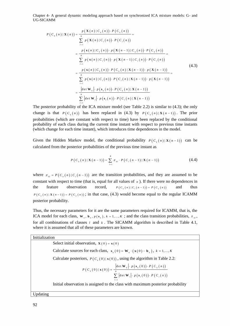
Chapter 4- A general dynamic modeling approach based on synchronized ICA mixture models: G- and
UG-SICAMM
92
1
1
1
1
||
|
| 1 |
| 1 |
| | 1 1
| | 1 1
d e t | 1
d e t | 1
k k
k K
l l
l
k k k
K
l l l
l
k k
K
l l
l
k k k
K
l l l
l
p n C n P C nP C n n
p n C n P C n
p n C n p n C n P C n
p n C n p n C n P C n
p n C n P C n n p n
p n C n P C n n p n
p n P C n n
p n P C n n
XX
X
x X
x X
x X X
x X X
W s X
W s X
(4.3)
The posterior probability of the ICA mixture model (see Table 2.2) is similar to (4.3); the only
change is that kP C n has been replaced in (4.3) by | 1
kP C n n X . The prior
probabilities (which are constant with respect to time) have been replaced by the conditional
probability of each class during the current time instant with respect to previous time instants
(which change for each time instant), which introduces time dependences in the model.
Given the Hidden Markov model, the conditional probability | 1k
P C n n X can be
calculated from the posterior probabilities of the previous time instant as
1
| 1 1 | 1
K
k k l l
l
P C n n P C n n
X X (4.4)
where | 1kl k l
P C n C n are the transition probabilities, and they are assumed to be
constant with respect to time (that is, equal for all values of n ). If there were no dependences in
the feature observation record, | 1k l k
P C n C n P C n and thus
| 1k k
P C n n P C n X ; in that case, (4.3) would become equal to the regular ICAMM
posterior probability.
Thus, the necessary parameters for it are the same parameters required for ICAMM, that is, the
ICA model for each class, , , , 1, ... ,k k k
p k KW b s ; and the class transition probabilities, k l
,
for all combinations of classes l and k . The SICAMM algorithm is described in Table 4.1,
where it is assumed that all of these parameters are known.
Initialization
Select initial observation, 0 0X x
Calculate sources for each class, 0 0k k k
s W x b , 1, ...,k K
Calculate posteriors, 0 | 0k
P C x , using the algorithm in Table 2.2:
1
d e t 00 | 0
d e t 0
k k k
k K
l l l
l
p P C nP C
p P C n
W sx
W s
Initial observation is assigned to the class with maximum posterior probability
Updating
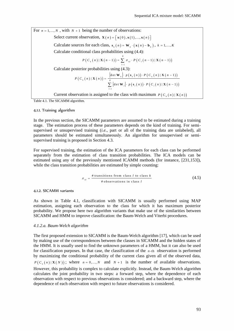
Sequential ICA mixture model: SICAMM
93
For 1, ...,n N , with 1N being the number of observations:
Select current observation, 0 , 1 , ...,n n
X x x x
Calculate sources for each class, k k kn n s W x b , 1, ...,k K
Calculate conditional class probabilities using (4.4):
1
| 1 1 | 1
K
k k l l
l
P C n n P C n n
X X
Calculate posterior probabilities using (4.3):
1
d e t | 1|
d e t | 1
k k k
k K
l l l
l
p n P C n nP C n n
p n P C n n
W s XX
W s X
Current observation is assigned to the class with maximum |k
P C n nX
Table 4.1. The SICAMM algorithm.
4.1.1. Training algorithm
In the previous section, the SICAMM parameters are assumed to be estimated during a training
stage. The estimation process of these parameters depends on the kind of training. For semi-
supervised or unsupervised training (i.e., part or all of the training data are unlabeled), all
parameters should be estimated simultaneously. An algorithm for unsupervised or semi-
supervised training is proposed in Section 4.3.
For supervised training, the estimation of the ICA parameters for each class can be performed
separately from the estimation of class transition probabilities. The ICA models can be
estimated using any of the previously mentioned ICAMM methods (for instance, [231,153]),
while the class transition probabilities are estimated by simple counting:
# tran s itio n s fro m c lass to c lass
# o b se rva tio n s in c lass k l
l k
l (4.5)
4.1.2. SICAMM variants
As shown in Table 4.1, classification with SICAMM is usually performed using MAP
estimation, assigning each observation to the class for which it has maximum posterior
probability. We propose here two algorithm variants that make use of the similarities between
SICAMM and HMM to improve classification: the Baum-Welch and Viterbi procedures.
4.1.2.a. Baum-Welch algorithm
The first proposed extension to SICAMM is the Baum-Welch algorithm [17], which can be used
by making use of the correspondences between the classes in SICAMM and the hidden states of
the HMM. It is usually used to find the unknown parameters of a HMM, but it can also be used
for classification purposes. In that case, the classification of the -thn observation is performed
by maximizing the conditional probability of the current class given all of the observed data,
|k
P C n NX ; where 0, ...,n N and 1N is the number of available observations.
However, this probability is complex to calculate explicitly. Instead, the Baum-Welch algorithm
calculates the joint probability in two steps: a forward step, where the dependence of each
observation with respect to previous observations is considered; and a backward step, where the
dependence of each observation with respect to future observations is considered.
Chapter 4- A general dynamic modeling approach based on synchronized ICA mixture models: G- and
UG-SICAMM
94
The forward step calculates the “forward” variable ,k k
n p n C n X , the joint
probability of class k and of all observations up to time n . Although it can be calculated
explicitly from (4.2), kn is usually calculated iteratively to improve the speed of the
algorithm. If we take the Bayes rule several times, and considering the Markov assumption, then
1
1
1
|
| 1 |
| | 1 1
| 1 | 1 1
| 1 , 1
| 1
k k k
k k k
k k
K
k k l l
l
K
k k l l
l
K
k k l l
l
n p n C n P C n
p n C n p n C n P C n
p n C n p C n n p n
p n C n p C n n p n
p n C n p n C n
p n C n n
X
x X
x X X
x X X
x X
x
(4.6)
where the initial value is 0 0 , 0 0 | 0 0k k k k
p C p C p C x x . The forward
step calculates all possible values of the forward variable for every time instant,
, 1, ... , , 1, ... ,k
n k K n N .
After the forward step is complete, the algorithm performs a backward step. This step calculates
the “backward” variable 1 , 2 , ...., |k k
n p n n N C n x x x , that is, the joint
probability of all future observations conditioned with respect to the current class. Once again,
the Baum-Welch algorithm calculates this variable iteratively; from the definition and applying
the HMM and the Markov assumption:
1
1
1
1 , 2 , .. . , |
1 , 2 , .. . , | 1
1 | 1 2 , .. . , | 1
1 | 1 1
l l
K
k l k
k
K
k l k k
k
K
k l k k
k
n p n n N C n
p n n N C n
p n C n p n N C n
p n C n n
x x x
x x x
x x x
x
(4.7)
where the initial value is 1 1, ...,l
N l K . As the name of the step suggests, this
calculation begins at the last observation and moves backwards until all the ln values are
calculated. Thus, the desired conditional expectation can be found as
1
|k k
k k N
l l
l
n nn p C n N
n n
X (4.8)
As explained above, the classification is performed by choosing the class with maximum kn
for each observation.
4.1.2.b. Viterbi algorithm
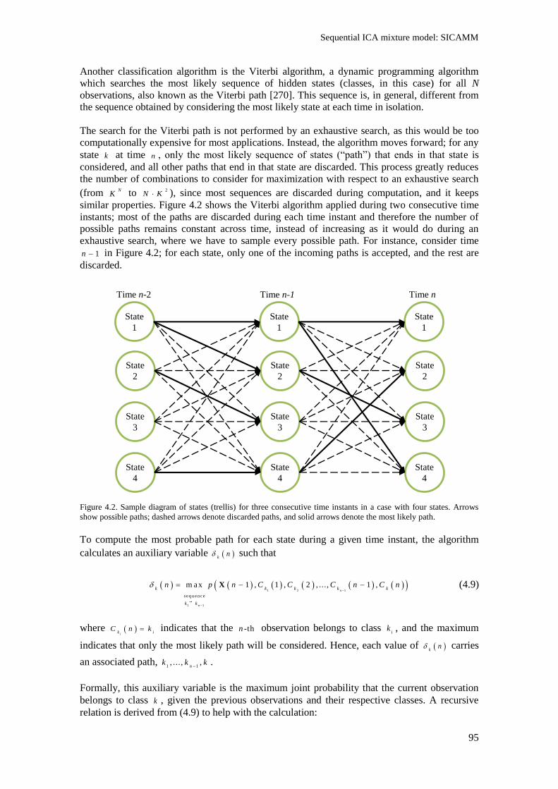
Sequential ICA mixture model: SICAMM
95
Another classification algorithm is the Viterbi algorithm, a dynamic programming algorithm
which searches the most likely sequence of hidden states (classes, in this case) for all N
observations, also known as the Viterbi path [270]. This sequence is, in general, different from
the sequence obtained by considering the most likely state at each time in isolation.
The search for the Viterbi path is not performed by an exhaustive search, as this would be too
computationally expensive for most applications. Instead, the algorithm moves forward; for any
state k at time n , only the most likely sequence of states (“path”) that ends in that state is
considered, and all other paths that end in that state are discarded. This process greatly reduces
the number of combinations to consider for maximization with respect to an exhaustive search
(from NK to 2
N K ), since most sequences are discarded during computation, and it keeps
similar properties. Figure 4.2 shows the Viterbi algorithm applied during two consecutive time
instants; most of the paths are discarded during each time instant and therefore the number of
possible paths remains constant across time, instead of increasing as it would do during an
exhaustive search, where we have to sample every possible path. For instance, consider time
1n in Figure 4.2; for each state, only one of the incoming paths is accepted, and the rest are
discarded.
Figure 4.2. Sample diagram of states (trellis) for three consecutive time instants in a case with four states. Arrows
show possible paths; dashed arrows denote discarded paths, and solid arrows denote the most likely path.
To compute the most probable path for each state during a given time instant, the algorithm
calculates an auxiliary variable kn such that
1 2 1
1 1
seq u en ce
m ax 1 , 1 , 2 , ..., 1 ,n
n
k k k k k
k k
n p n C C C n C n
X (4.9)
where i
k iC n k indicates that the -thn observation belongs to class
ik , and the maximum
indicates that only the most likely path will be considered. Hence, each value of kn carries
an associated path, 1 1, ..., ,
nk k k
.
Formally, this auxiliary variable is the maximum joint probability that the current observation
belongs to class k , given the previous observations and their respective classes. A recursive
relation is derived from (4.9) to help with the calculation:
State
1
State
2
State
3
State
4
State
1
State
2
State
3
State
4
Time n-2 Time n-1
State
1
State
2
State
3
State
4
Time n

Chapter 4- A general dynamic modeling approach based on synchronized ICA mixture models: G- and
UG-SICAMM
96
1
1 1 | 1 m a xk k k l l
l K
n p n C n n
x (4.10)
with initial value 0 0 , 0 0 | 0 0k k k k
p C p C p C x x . Once all the kN
have been calculated, there are K possible paths, each one ending in a different state kC N .
The algorithm then selects the path with maximum kN and returns the associated sequence
of states 1 1, ..., ,
nk k k
(as seen (4.9) and commented above) as the classification of the
observations.
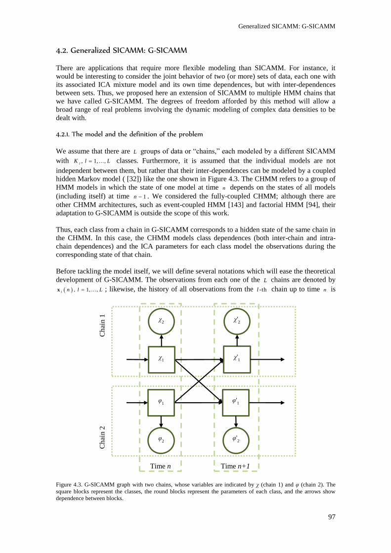
Generalized SICAMM: G-SICAMM
97
4.2. Generalized SICAMM: G-SICAMM
There are applications that require more flexible modeling than SICAMM. For instance, it
would be interesting to consider the joint behavior of two (or more) sets of data, each one with
its associated ICA mixture model and its own time dependences, but with inter-dependences
between sets. Thus, we proposed here an extension of SICAMM to multiple HMM chains that
we have called G-SICAMM. The degrees of freedom afforded by this method will allow a
broad range of real problems involving the dynamic modeling of complex data densities to be
dealt with.
4.2.1. The model and the definition of the problem
We assume that there are L groups of data or “chains,” each modeled by a different SICAMM
with , 1, ...,l
K l L classes. Furthermore, it is assumed that the individual models are not
independent between them, but rather that their inter-dependences can be modeled by a coupled
hidden Markov model ( [32]) like the one shown in Figure 4.3. The CHMM refers to a group of
HMM models in which the state of one model at time n depends on the states of all models
(including itself) at time 1n . We considered the fully-coupled CHMM; although there are
other CHMM architectures, such as event-coupled HMM [143] and factorial HMM [94], their
adaptation to G-SICAMM is outside the scope of this work.
Thus, each class from a chain in G-SICAMM corresponds to a hidden state of the same chain in
the CHMM. In this case, the CHMM models class dependences (both inter-chain and intra-
chain dependences) and the ICA parameters for each class model the observations during the
corresponding state of that chain.
Before tackling the model itself, we will define several notations which will ease the theoretical
development of G-SICAMM. The observations from each one of the L chains are denoted by
, 1, .. . ,l
n l Lx ; likewise, the history of all observations from the -thl chain up to time n is
Figure 4.3. G-SICAMM graph with two chains, whose variables are indicated by χ (chain 1) and φ (chain 2). The
square blocks represent the classes, the round blocks represent the parameters of each class, and the arrows show
dependence between blocks.
Time n Time n+1
χ'1
φ'1
χ1
φ1
φ2
χ2
φ'2
χ'2
Chai
n 1
C
hai
n 2
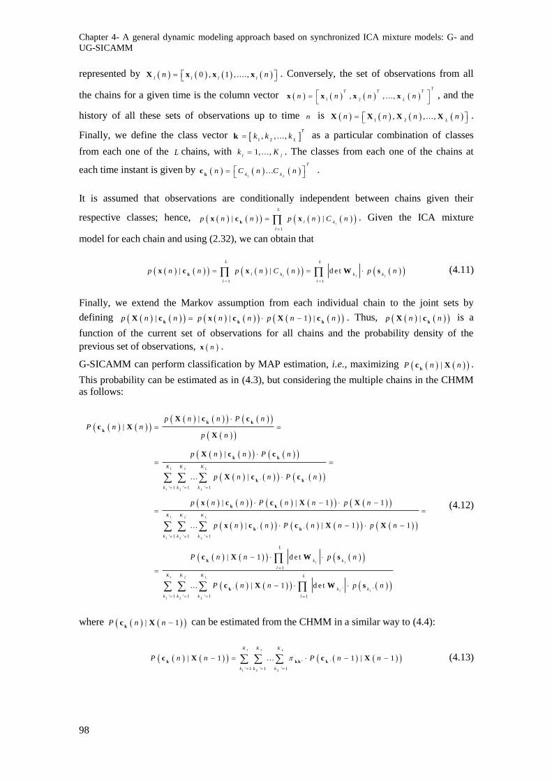
Chapter 4- A general dynamic modeling approach based on synchronized ICA mixture models: G- and
UG-SICAMM
98
represented by 0 , 1 , ....,l l l l
n n
X x x x . Conversely, the set of observations from all
the chains for a given time is the column vector 1 2, , . . . ,
TT T T
Ln n n n
x x x x , and the
history of all these sets of observations up to time n is 1 2, , ...,
Ln n n n
X X X X .
Finally, we define the class vector 1 2, , ...,
T
Lk k kk as a particular combination of classes
from each one of the L chains, with 1, ...,l l
k K . The classes from each one of the chains at
each time instant is given by 1
...L
T
k kn C n C n
kc .
It is assumed that observations are conditionally independent between chains given their
respective classes; hence, 1
| |l
L
l k
l
p n n p n C n
kx c x . Given the ICA mixture
model for each chain and using (2.32), we can obtain that
1 1
| | d e tl l l
L L
l k k k
l l
p n n p n C n p n
kx c x W s (4.11)
Finally, we extend the Markov assumption from each individual chain to the joint sets by
defining | | 1 |p n n p n n p n n k k k
X c x c X c . Thus, |p n nk
X c is a
function of the current set of observations for all chains and the probability density of the
previous set of observations, nx .
G-SICAMM can perform classification by MAP estimation, i.e., maximizing |P n nk
c X .
This probability can be estimated as in (4.3), but considering the multiple chains in the CHMM
as follows:
1 2
1 2
1 2
1 2
' '
' 1 ' 1 ' 1
' '
' 1 ' 1 ' 1
1
'
||
|
. . . |
| | 1 1
... | | 1 1
| 1 d e t
.. . | 1 d e
L
L
L
L
l l
K K K
k k k
K K K
k k k
L
k k
l
p n n P nP n n
p n
p n n P n
p n n P n
p n n P n n p n
p n n P n n p n
P n n p n
P n n
k k
k
k k
k k
k k
k k
k
k
X c cc X
X
X c c
X c c
x c c X X
x c c X X
c X W s
c X 1 2
1 2
' '
' 1 ' 1 ' 1 1
t
L
l l
L
K K K L
k k
k k k l
p n
W s
(4.12)
where | 1P n n k
c X can be estimated from the CHMM in a similar way to (4.4):
1 2
1 2
'
' 1 ' 1 ' 1
| 1 .. . 1 | 1
L
L
K K K
k k k
P n n P n n
k k k ' kc X c X (4.13)
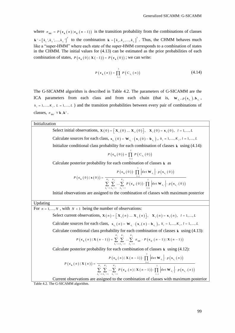
Generalized SICAMM: G-SICAMM
99
where | 1P n n kk' k k'
c c is the transition probability from the combinations of classes
1 2' ', ', ..., '
T
Lk k kk to the combination 1 2
, , ...,T
Lk k kk . Thus, the CHMM behaves much
like a “super-HMM” where each state of the super-HMM corresponds to a combination of states
in the CHMM. The initial values for (4.13) can be estimated as the prior probabilities of each
combination of states, 0 | 1 0P P k k
c X c ; we can write:
1
l
L
k
l
P n P C n
kc (4.14)
The G-SICAMM algorithm is described in Table 4.2. The parameters of G-SICAMM are the
ICA parameters from each class and from each chain (that is, , ,l l l
k k kpW s b ,
1, ..., , 1, ... ,l l
k K L L ) and the transition probabilities between every pair of combinations of
classes, , k k '
k k ' .
Initialization
Select initial observations, 10 0 ... 0 , 0 0 , 1, ...,
L l ll L
X X X X x
Calculate sources for each class, 0 0l l l
k k l k s W x b , 1, ..., , 1, ...,
l lk K l L
Initialize conditional class probability for each combination of classes k using (4.14):
1
0 0l
L
k
l
P P C
kc
Calculate posterior probability for each combination of classes k as
1 2
1 2
1
' ' '
' 1 ' 1 ' 1 1
0 d e t 0
0 | 0
... 0 d e t 0
l l
L
l l
L
L
k k
l
K K K L
k k
k k k l
P p
P
P p
k
k
k
c W s
c x
c W s
Initial observations are assigned to the combination of classes with maximum posterior
Updating
For 1, ...,n N , with 1N being the number of observations:
Select current observations, 1... , , 1, ...,
L l ln n n n n l L
X X X X x
Calculate sources for each class, l l l
k k l kn n s W x b , 1, ..., , 1, ...,
l lk K l L
Calculate conditional class probability for each combination of classes k using (4.13):
1 2
1 2
'
' 1 ' 1 ' 1
| 1 .. . 1 | 1
L
L
K K K
k k k
P n n P n n
k k k ' kc X c X
Calculate posterior probability for each combination of classes k using (4.12):
1 2
1 2
1
' ' '
' 1 ' 1 ' 1 1
| 1 d e t
|
. . . | 1 d e t
l l
L
l l
L
L
k k
l
K K K L
k k
k k k l
P n n p n
P n n
P n n p n
k
k
k
c X W s
c X
c X W s
Current observations are assigned to the combination of classes with maximum posterior Table 4.2. The G-SICAMM algorithm.
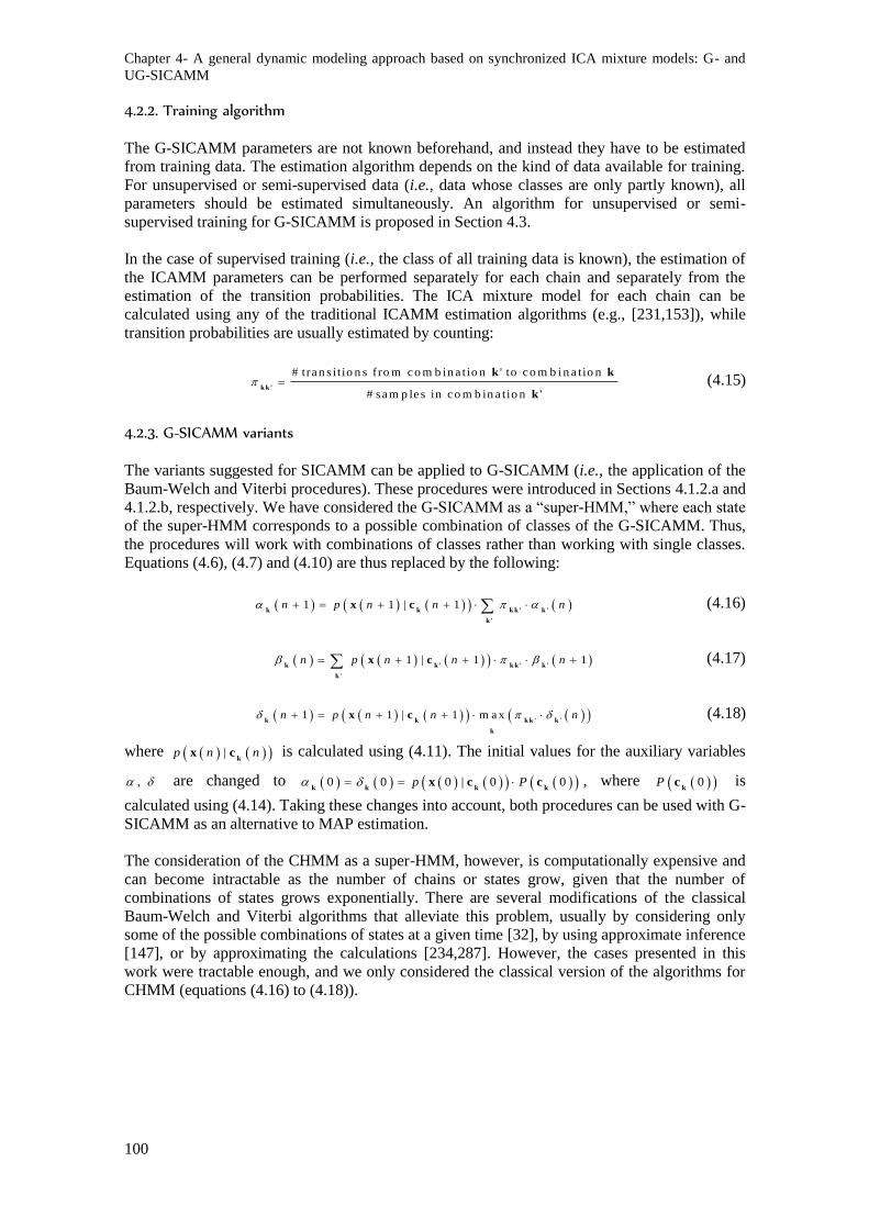
Chapter 4- A general dynamic modeling approach based on synchronized ICA mixture models: G- and
UG-SICAMM
100
4.2.2. Training algorithm
The G-SICAMM parameters are not known beforehand, and instead they have to be estimated
from training data. The estimation algorithm depends on the kind of data available for training.
For unsupervised or semi-supervised data (i.e., data whose classes are only partly known), all
parameters should be estimated simultaneously. An algorithm for unsupervised or semi-
supervised training for G-SICAMM is proposed in Section 4.3.
In the case of supervised training (i.e., the class of all training data is known), the estimation of
the ICAMM parameters can be performed separately for each chain and separately from the
estimation of the transition probabilities. The ICA mixture model for each chain can be
calculated using any of the traditional ICAMM estimation algorithms (e.g., [231,153]), while
transition probabilities are usually estimated by counting:
# tran s itio n s fro m co m b in a tio n ' to co m b i n a tio n
# sam p le s in co m b in a tio n '
k k '
k k
k (4.15)
4.2.3. G-SICAMM variants
The variants suggested for SICAMM can be applied to G-SICAMM (i.e., the application of the
Baum-Welch and Viterbi procedures). These procedures were introduced in Sections 4.1.2.a and
4.1.2.b, respectively. We have considered the G-SICAMM as a “super-HMM,” where each state
of the super-HMM corresponds to a possible combination of classes of the G-SICAMM. Thus,
the procedures will work with combinations of classes rather than working with single classes.
Equations (4.6), (4.7) and (4.10) are thus replaced by the following:
1 1 | 1n p n n n k k k k ' k '
k '
x c (4.16)
1 | 1 1n p n n n k k ' k k ' k '
k '
x c (4.17)
1 1 | 1 m a xn p n n n k k k k ' k '
k
x c (4.18)
where |p n nk
x c is calculated using (4.11). The initial values for the auxiliary variables
, are changed to 0 0 0 | 0 0p P k k k k
x c c , where 0Pk
c is
calculated using (4.14). Taking these changes into account, both procedures can be used with G-
SICAMM as an alternative to MAP estimation.
The consideration of the CHMM as a super-HMM, however, is computationally expensive and
can become intractable as the number of chains or states grow, given that the number of
combinations of states grows exponentially. There are several modifications of the classical
Baum-Welch and Viterbi algorithms that alleviate this problem, usually by considering only
some of the possible combinations of states at a given time [32], by using approximate inference
[147], or by approximating the calculations [234,287]. However, the cases presented in this
work were tractable enough, and we only considered the classical version of the algorithms for
CHMM (equations (4.16) to (4.18)).
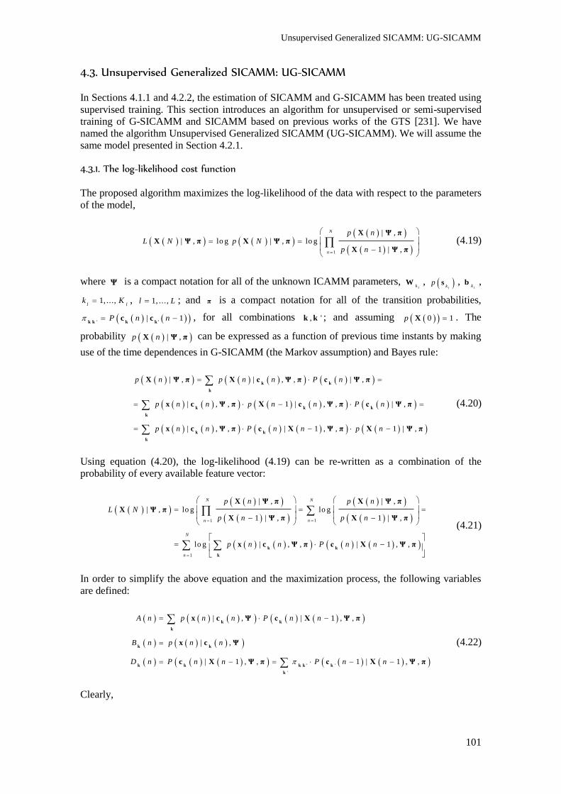
Unsupervised Generalized SICAMM: UG-SICAMM
101
4.3. Unsupervised Generalized SICAMM: UG-SICAMM
In Sections 4.1.1 and 4.2.2, the estimation of SICAMM and G-SICAMM has been treated using
supervised training. This section introduces an algorithm for unsupervised or semi-supervised
training of G-SICAMM and SICAMM based on previous works of the GTS [231]. We have
named the algorithm Unsupervised Generalized SICAMM (UG-SICAMM). We will assume the
same model presented in Section 4.2.1.
4.3.1. The log-likelihood cost function
The proposed algorithm maximizes the log-likelihood of the data with respect to the parameters
of the model,
1
| ,| , lo g | , lo g
1 | ,
N
n
p nL N p N
p n
X Ψ π
X Ψ π X Ψ πX Ψ π
(4.19)
where Ψ is a compact notation for all of the unknown ICAMM parameters, l
kW ,
lk
p s , l
kb ,
1, ...,l l
k K , 1, ...,l L ; and π is a compact notation for all of the transition probabilities,
'| 1P n n
k k k k'c c , for all combinations , 'k k ; and assuming 0 1p X . The
probability | ,p nX Ψ π can be expressed as a function of previous time instants by making
use of the time dependences in G-SICAMM (the Markov assumption) and Bayes rule:
| , | , , | ,
| , , 1 | , , | ,
| , , | 1 , , 1 | ,
p n p n n P n
p n n p n n P n
p n n P n n p n
k k
k
k k k
k
k k
k
X Ψ π X c Ψ π c Ψ π
x c Ψ π X c Ψ π c Ψ π
x c Ψ π c X Ψ π X Ψ π
(4.20)
Using equation (4.20), the log-likelihood (4.19) can be re-written as a combination of the
probability of every available feature vector:
11
1
| , | ,| , lo g lo g
1 | , 1 | ,
lo g | , , | 1 , ,
N N
nn
N
n
p n p nL N
p n p n
p n n P n n
k k
k
X Ψ π X Ψ πX Ψ π
X Ψ π X Ψ π
x c Ψ π c X Ψ π
(4.21)
In order to simplify the above equation and the maximization process, the following variables
are defined:
'
'
| , | 1 , ,
| ,
| 1 , , 1 | 1 , ,
A n p n n P n n
B n p n n
D n P n n P n n
k k
k
k k
k k k k ' k
k
x c Ψ c X Ψ π
x c Ψ
c X Ψ π c X Ψ π
(4.22)
Clearly,
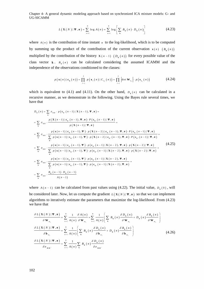
Chapter 4- A general dynamic modeling approach based on synchronized ICA mixture models: G- and
UG-SICAMM
102
1 1
| , lo g lo g
N N
n n
L N A n B n D n
k k
k
X Ψ π (4.23)
where A n is the contribution of time instant n to the log-likelihood, which is to be computed
by summing up the product of the contribution of the current observation nx B nk
multiplied by the contribution of the history 1n X D nk
for every possible value of the
class vector k . B nk
can be calculated considering the assumed ICAMM and the
independence of the observations conditioned to the classes:
1 1
| | d e tl l l
L L
l k k k
l l
p n n p n C n p n
kx c x W s (4.24)
which is equivalent to (4.1) and (4.11). On the other hand, D nk
can be calculated in a
recursive manner, as we demonstrate in the following. Using the Bayes rule several times, we
have that
'
'
' '
'
' ' '
' '' '' ''
''
'
1 | 1 , ,
1 | 1 , , 1 | ,
1 | ,
1 | 1 , 2 | 1 , , 1 | ,
1 | 1 , 2 | 1 , , 1 | ,
1 | 1 ,
D n p n n
p n n P n
p n
p n n p n n P n
p n n p n n P n
p n n
k k k ' k
k
k k
k k '
k
k k k
k k '
k k k k
k
k
k k '
c X Ψ π
X c Ψ π c Ψ π
X Ψ π
x c Ψ X c Ψ π c Ψ π
x c Ψ X c Ψ π c Ψ π
x c Ψ
'
' '' ''
''
' '
' '' ''
''
'
1 | 2 , , 2 | ,
1 | 1 , 1 | 2 , , 2 | ,
1 | 1 , 1 | 2 , ,
1 | 1 , 1 | 2 , ,
1 1
1
p n n p n
p n n p n n p n
p n n p n n
p n n p n n
B n D n
A n
k
k k k
k
k k
k k '
k k k
k
k ' k '
k k '
k
c X Ψ π X Ψ π
x c Ψ c X Ψ π X Ψ π
x c Ψ c X Ψ π
x c Ψ c X Ψ π
(4.25)
where 1A n can be calculated from past values using (4.22). The initial value, 0Dk
, will
be considered later. Now, let us compute the gradient | ,L NX Ψ π so that we can implement
algorithms to iteratively estimate the parameters that maximize the log-likelihood. From (4.23)
we have that
1 1
1
1' '
| , 1 1
| , 1
| , 1
l l l l
l l l
N N
n nm m m m
N
nm m m
N
n
L N A n D n B nB n D n
A n A n
L N D n B nB n D n
A n
L N D nB n
A n
k k
k k
k
k k
k k
k
k
k
km m m m
X Ψ π
W W W W
X Ψ π
b b b
X Ψ π
(4.26)
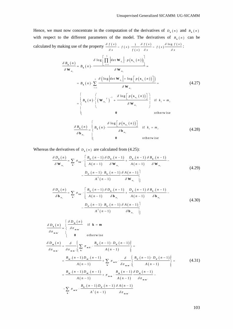
Unsupervised Generalized SICAMM: UG-SICAMM
103
Hence, we must now concentrate in the computation of the derivatives of D nk
and B nk
with respect to the different parameters of the model. The derivatives of B nk
can be
calculated by making use of the property
lo g1f x f x f xf x f x
x f x x x
:
1
1
1
lo g d e t
lo g d e t lo g
lo g
if
o th e rw is e
l l
l l
l l
l
l
l
l
L
k k
l
m m
Lk k
l m
mT
m l l
m
p nB n
B n
p n
B n
p n
B n k m
k
k
k
k
W s
W W
W s
W
s
WW
0
(4.27)
lo g
if
o th e rw ise
l
l
l
m
l l
m
m
p nB n B n k m
k k
s
bb
0
(4.28)
Whereas the derivatives of D nk
are calculated from (4.25):
' ' ' '
'
'
' '
2
1 1 1 1
1 1
1 1 1
1
l l l
l
m m m
m
D n B n D n D n B n
A n A n
D n B n A n
A n
k k k k k
k k
k
k k
W W W
W
(4.29)
' ' ' '
'
'
' '
2
1 1 1 1
1 1
1 1 1
1
l l l
l
m m m
m
D n B n D n D n B n
A n A n
D n B n A n
A n
k k k k k
k k
k
k k
b b b
b
(4.30)
'
'
'' '
' '
' '
' '
'
i f
o th e rw is e
1 1
1
1 1 1 1
1 1
1 1 1 1
1 1
D nD n
D n B n D n
A n
B n D n B n D n
A n A n
B n D n B n D n
A n A n
m
k
m m
m m
m k ' k '
m k '
km m m m
m m k ' k '
m k '
k m m
m m m m
m m
m m
m k
k m
0
' '
2
' '
1 1 1
1
B n D n A n
A n
k k
'
k m m
(4.31)
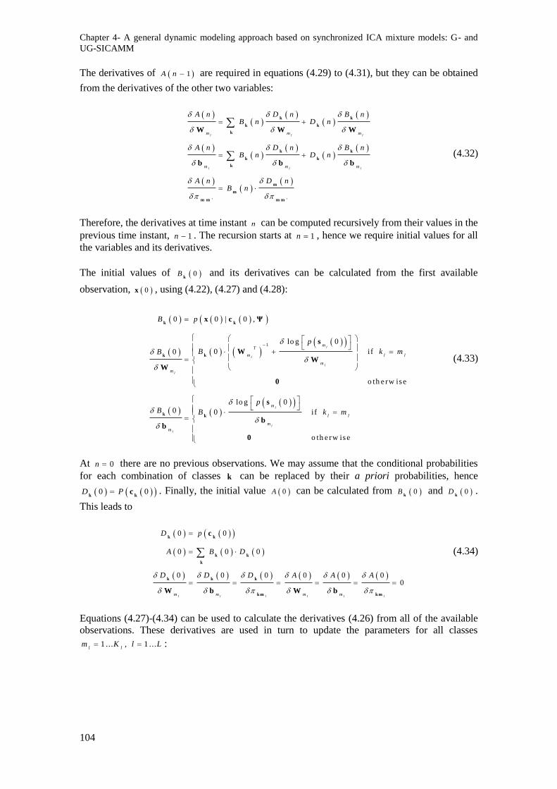
Chapter 4- A general dynamic modeling approach based on synchronized ICA mixture models: G- and
UG-SICAMM
104
The derivatives of 1A n are required in equations (4.29) to (4.31), but they can be obtained
from the derivatives of the other two variables:
' '
l l l
l l l
m m m
m m m
A n D n B nB n D n
A n D n B nB n D n
A n D nB n
k k
k k
k
k k
k k
k
m
m
m m m m
W W W
b b b
(4.32)
Therefore, the derivatives at time instant n can be computed recursively from their values in the
previous time instant, 1n . The recursion starts at 1n , hence we require initial values for all
the variables and its derivatives.
The initial values of 0Bk
and its derivatives can be calculated from the first available
observation, 0x , using (4.22), (4.27) and (4.28):
1
0 0 | 0 ,
lo g 0
0 if 0
o th e rw ise
lo g 00 0 if
o th e rw ise
l
l
l
l
l
l
l
mT
m l l
m
m
m
l l
m
m
B p
p
B k mB
pB B k m
k k
kk
k k
x c Ψ
s
WW
W
0
s
bb
0
(4.33)
At 0n there are no previous observations. We may assume that the conditional probabilities
for each combination of classes k can be replaced by their a priori probabilities, hence
0 0D Pk k
c . Finally, the initial value 0A can be calculated from 0Bk
and 0Dk
.
This leads to
0 0
0 0 0
0 0 0 0 0 00
l l l l l lm m m m
D p
A B D
D D D A A A
k k
k k
k
k k k
k m k m
c
W b W b
(4.34)
Equations (4.27)-(4.34) can be used to calculate the derivatives (4.26) from all of the available
observations. These derivatives are used in turn to update the parameters for all classes
1 ... , 1 ...l l
m K l L :
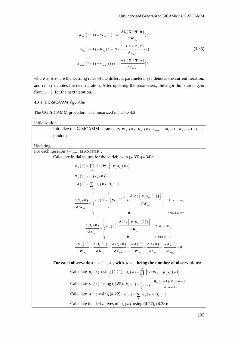
Unsupervised Generalized SICAMM: UG-SICAMM
105
' '
'
/ ,1
/ ,1
/ ,1
l l
l
l l
l
m m
m
m m
m
Li i i
Li i i
Li i i
m m m m
m m
X Ψ πW W
W
X Ψ πb b
b
X Ψ π
(4.35)
where , , are the learning rates of the different parameters, i denotes the current iteration,
and 1i denotes the next iteration. After updating the parameters, the algorithm starts again
from 0n for the next iteration.
4.3.2. UG-SICAMM algorithm
The UG-SICAMM procedure is summarized in Table 4.3.
Initialization
Initialize the G-SICAMM parameters '0 , 0 ,
l lm m
m m
W b , 1 ... , 1 ...l l
m K l L at
random
Updating
For each iteration 1, ..., M A X IT E Ri ,
Calculate initial values for the variables in (4.33)-(4.34):
1
0 d e t 0
0 0
0 0 0
l l
L
k k
l
B p
D p
A B D
k
k k
k k
k
W s
c
1
lo g 0
0 if 0
o th e rw is e
l
l
l
l
mT
m l l
m
m
p
B k mB
kk
s
WW
W
0
lo g 0
0 0 if
o th e rw ise
l
l
l
m
l l
m
m
pB B k m
k k
s
bb
0
0 0 0 0 0 00
l l l l l lm m m m
D D D A A A
k k k
km kmW b W b
For each observation 1, ...,n N , with 1N being the number of observations:
Calculate k
B n using (4.11), 1
d e tl l
L
k k k
l
B n p n
W s
Calculate k
D n using (4.25),
'
1 1
1
B n D nD n
A n
k ' k '
k k k '
k
Calculate A n using (4.22), A n B n D n k k
k
Calculate the derivatives of kB n using (4.27), (4.28):
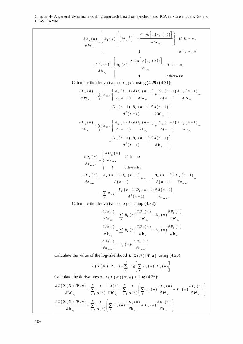
Chapter 4- A general dynamic modeling approach based on synchronized ICA mixture models: G- and
UG-SICAMM
106
1
lo g
if
o th e rw is e
l
l
l
l
mT
m l l
m
m
p n
B n k mB n
kk
s
WW
W
0
lo g
if
o th e rw ise
l
l
l
m
l l
m
m
p nB n B n k m
k k
s
bb
0
Calculate the derivatives of kD n using (4.29)-(4.31):
' ' ' '
'
'
' '
2
1 1 1 1
1 1
1 1 1
1
l l l
l
m m m
m
D n B n D n D n B n
A n A n
D n B n A n
A n
k k k k k
k k
k
k k
W W W
W
' ' ' '
'
'
' '
2
1 1 1 1
1 1
1 1 1
1
l l l
l
m m m
m
D n B n D n D n B n
A n A n
D n B n A n
A n
k k k k k
k k
k
k k
b b b
b
'
'
' '
' '
' '
2
' '
i f
o th e rw is e
1 1 1 1
1 1
1 1 1
1
D nD n
D n B n D n B n D n
A n A n
B n D n A n
A n
m
k
m m
m m
m m m m m
m m
m m m m
k k
m k '
k m m
k m
0
Calculate the derivatives of A n using (4.32):
l l lm m m
A n D n B nB n D n
k k
k k
kW W W
l l lm m m
A n D n B nB n D n
k k
k k
kb b b
' '
A n D nB n
m
m
m m m m
Calculate the value of the log-likelihood |L NX Ψ , π using (4.23):
1
| , lo g
N
n
L N B n D n
k k
k
X Ψ π
Calculate the derivatives of |L NX Ψ , π using (4.26):
1 1
1
| , 1 1
| , 1
l l l l
l l l
N N
n nm m m m
N
nm m m
L N A n D n B nB n D n
A n A n
L N D n B nB n D n
A n
k k
k k
k
k k
k k
k
X Ψ π
W W W W
X Ψ π
b b b
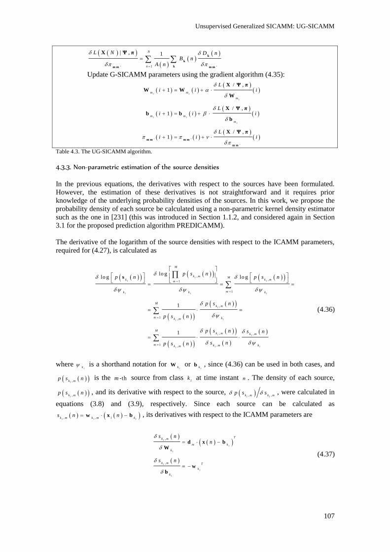
Unsupervised Generalized SICAMM: UG-SICAMM
107
1' '
| , 1N
n
L N D nB n
A n
k
k
km m m m
X Ψ π
Update G-SICAMM parameters using the gradient algorithm (4.35):
' '
'
/ ,1
/ ,1
/ ,1
l l
l
l l
l
m m
m
m m
m
Li i i
Li i i
Li i i
m m m m
m m
X Ψ πW W
W
X Ψ πb b
b
X Ψ π
Table 4.3. The UG-SICAMM algorithm.
4.3.3. Non-parametric estimation of the source densities
In the previous equations, the derivatives with respect to the sources have been formulated.
However, the estimation of these derivatives is not straightforward and it requires prior
knowledge of the underlying probability densities of the sources. In this work, we propose the
probability density of each source be calculated using a non-parametric kernel density estimator
such as the one in [231] (this was introduced in Section 1.1.2, and considered again in Section
3.1 for the proposed prediction algorithm PREDICAMM).
The derivative of the logarithm of the source densities with respect to the ICAMM parameters,
required for (4.27), is calculated as
,,
1
1
,
1,
, ,
1 ,,
lo glo g lo g
1
1
l
l l
l l l
l
ll
l l
l ll
M
k m Mk k m
m
mk k k
Mk m
m kk m
Mk m k m
m k m kk m
p s np n p s n
p s n
p s n
p s n s n
s np s n
s
(4.36)
where l
k is a shorthand notation for
lk
W or l
kb , since (4.36) can be used in both cases, and
,l
k mp s n is the -thm source from class
lk at time instant n . The density of each source,
,l
k mp s n , and its derivative with respect to the source, , ,
l lk m k m
p s s , were calculated in
equations (3.8) and (3.9), respectively. Since each source can be calculated as
, ,l l l
k m k m l ks n n w x b , its derivatives with respect to the ICAMM parameters are
,
,
l
l
l
l
l
l
Tk m
m k
k
k m T
k
k
s nn
s n
d x bW
wb
(4.37)
Chapter 4- A general dynamic modeling approach based on synchronized ICA mixture models: G- and
UG-SICAMM
108
where m
d is a column vector of zeros with a 1 in its -thm position. Thus, finally, the derivatives
of the logarithm of the densities of the sources are:
,
1 ,,
,
1 ,,
lo g 1
lo g 1( 1)
l l
l
l ll
l l
l l
l l l
l ll
MTk k m
m k
mk k mk m
T
k k
Mk k m T T
k k k
mk k mk m
p n p s n
d ns np s n
f n n
p n p s n
f ns np s n
s
x bW
s x b
s
w W sb
(4.38)
where l
kf ns is a column vector whose -thm element is equal to
,
,,
1l
ll
k m
k mk m
p s
sp s
,
1, ...,m M . By substituting (4.38) in (4.27) and (4.28), we obtain that
1
if
o th e rw ise
l l l
l
TT
m m m l l
m
B n f n n k mB n
kkW s x b
W0
(4.39)
i f
o th e rw ise
l l
l
T
m m l l
m
B n f n k mB n
kkW s
b 0
(4.40)
Equation (4.39) can be replaced by the natural gradient, a variation of the regular gradient which
has demonstrated good convergence properties [7]. In that case, the gradient with respect to the
de-mixing matrices becomes
i f
o th e rw ise
l l
ll
l l l
T
m m
mm
T
m m m l l
B n B n
B n f n n k m
k k
k
W WWW
I s s W
0
(4.41)
4.3.4. Semi-supervised training
Let us consider a hybrid case with semi-supervised training, in which we could define some
prior knowledge about some observations, such as their class. For instance, if lnx is known
to belong to class 'l
k , then | 1P n n m
c x if 'l l
k k , and | 0P n n m
c x otherwise.
In that case, we can omit the calculation of B nm
for all combinations that do not include class
'l
k :
i f '
| ,0 o th e rw is e
l lB n k k
B n p n n
k
k kx c Ψ (4.42)
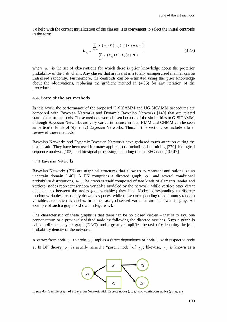
State of the art methods
109
To help with the correct initialization of the classes, it is convenient to select the initial centroids
in the form
| ,
| ,
l
l
l
l m l
n n s
m
m l
n n s
n P c n n
P c n n
x x Ψ
b
x Ψ
(4.43)
where n s is the set of observations for which there is prior knowledge about the posterior
probability of the -thl chain. Any classes that are learnt in a totally unsupervised manner can be
initialized randomly. Furthermore, the centroids can be estimated using this prior knowledge
about the observations, replacing the gradient method in (4.35) for any iteration of the
procedure.
4.4. State of the art methods
In this work, the performance of the proposed G-SICAMM and UG-SICAMM procedures are
compared with Bayesian Networks and Dynamic Bayesian Networks [140] that are related
state-of-the-art methods. These methods were chosen because of the similarities to G-SICAMM,
although Bayesian Networks are very varied in nature: in fact, HMM and CHMM can be seen
as particular kinds of (dynamic) Bayesian Networks. Thus, in this section, we include a brief
review of these methods.
Bayesian Networks and Dynamic Bayesian Networks have gathered much attention during the
last decade. They have been used for many applications, including data mining [279], biological
sequence analysis [102], and biosignal processing, including that of EEG data [107,47].
4.4.1. Bayesian Networks
Bayesian Networks (BN) are graphical structures that allow us to represent and rationalize an
uncertain domain [140]. A BN comprises a directed graph, G , and several conditional
probability distributions, . The graph is itself composed of two kinds of elements, nodes and
vertices; nodes represent random variables modeled by the network, while vertices state direct
dependences between the nodes (i.e., variables) they link. Nodes corresponding to discrete
random variables are usually drawn as squares, while those corresponding to continuous random
variables are drawn as circles. In some cases, observed variables are shadowed in gray. An
example of such a graph is shown in Figure 4.4.
One characteristic of these graphs is that there can be no closed circles – that is to say, one
cannot return to a previously-visited node by following the directed vertices. Such a graph is
called a directed acyclic graph (DAG), and it greatly simplifies the task of calculating the joint
probability density of the network.
A vertex from node i
to node j
implies a direct dependence of node j with respect to node
i . In BN theory, i
is usually named a “parent node” of j
; likewise, j
is known as a
Figure 4.4. Sample graph of a Bayesian Network with discrete nodes (χ1, χ2) and continuous nodes (χ3, χ4, χ5).
χ3
χ1χ4
χ5χ2
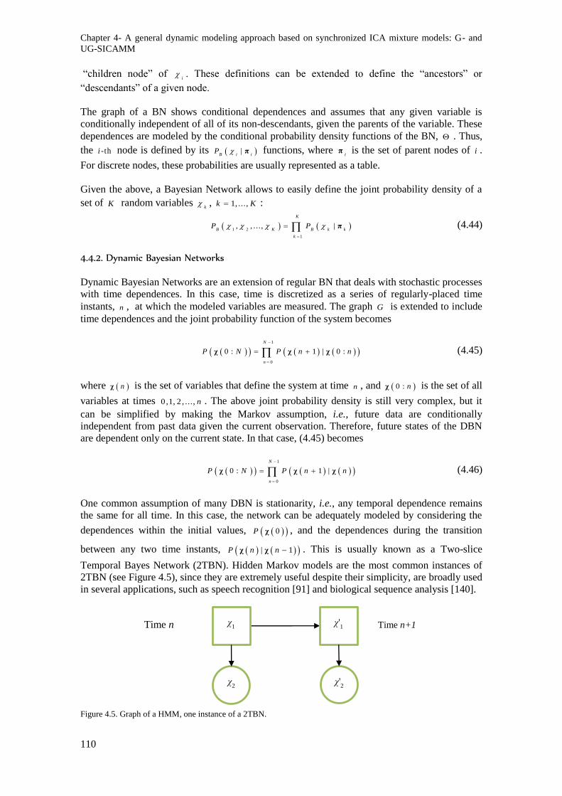
Chapter 4- A general dynamic modeling approach based on synchronized ICA mixture models: G- and
UG-SICAMM
110
“children node” of i
. These definitions can be extended to define the “ancestors” or
“descendants” of a given node.
The graph of a BN shows conditional dependences and assumes that any given variable is
conditionally independent of all of its non-descendants, given the parents of the variable. These
dependences are modeled by the conditional probability density functions of the BN, . Thus,
the -thi node is defined by its |B i i
P π functions, where i
π is the set of parent nodes of i .
For discrete nodes, these probabilities are usually represented as a table.
Given the above, a Bayesian Network allows to easily define the joint probability density of a
set of K random variables k
, 1, ...,k K :
1 2
1
, , . . . , |
K
B K B k k
k
P P
π (4.44)
4.4.2. Dynamic Bayesian Networks
Dynamic Bayesian Networks are an extension of regular BN that deals with stochastic processes
with time dependences. In this case, time is discretized as a series of regularly-placed time
instants, n , at which the modeled variables are measured. The graph G is extended to include
time dependences and the joint probability function of the system becomes
1
0
0 : 1 | 0 :
N
n
P N P n n
χ χ χ (4.45)
where nχ is the set of variables that define the system at time n , and 0 : nχ is the set of all
variables at times 0,1, 2 , ..., n . The above joint probability density is still very complex, but it
can be simplified by making the Markov assumption, i.e., future data are conditionally
independent from past data given the current observation. Therefore, future states of the DBN
are dependent only on the current state. In that case, (4.45) becomes
1
0
0 : 1 |
N
n
P N P n n
χ χ χ (4.46)
One common assumption of many DBN is stationarity, i.e., any temporal dependence remains
the same for all time. In this case, the network can be adequately modeled by considering the
dependences within the initial values, 0P χ , and the dependences during the transition
between any two time instants, | 1P n n χ χ . This is usually known as a Two-slice
Temporal Bayes Network (2TBN). Hidden Markov models are the most common instances of
2TBN (see Figure 4.5), since they are extremely useful despite their simplicity, are broadly used
in several applications, such as speech recognition [91] and biological sequence analysis [140].
Figure 4.5. Graph of a HMM, one instance of a 2TBN.
Time n Time n+1 χ'1 χ
1
χ2 χ'
2

Simulations
111
4.5. Simulations
The proposed procedures were tested on simulated data before their application on real data that
will be studied in Chapter 6.
4.5.1. Measuring the distance between two G-SICAMMs
Some of the applications in this work require measuring the distance or difference between two
sets of G-SICAMM parameters, e.g., to compare two G-SICAMM calculated at different times.
However, given the novelty of these procedures, there is no commonly-used measure of the
similarity of two given models. Considering their parameter structure, it seems appropriate to
combine the similarity measures for Hidden Markov Models with those for ICA.
Any similarity measure used to compare ICA mixture models, including sequential models like
G-SICAMM, should take into account the indeterminacies or unknowns of ICA, i.e., the sources
are recovered in no particular order, and the sources are identified up to a scale factor (including
a sign), . In this work, two indicators were considered, the Amari index and the SIR. Both
indicators are typical in the comparison of ICA models. A third indicator, the probabilistic
distance, was considered in order to compare transition probabilities, thus completing the
comparison of G-SICAMM parameters.
In the following, the G-SICAMM parameters at time instants i
n and j
n will be denoted by the
super-indices i and j
, respectively, while the models will be referred to as i
and j
,
respectively. Note that, even though the formulation will assume two G-SICAMM, these
indicators can be used to compare two sets of SICAMM parameters by setting 1L .
4.5.1.a. Amari index
The Amari index is used to calculate the similarity of a given matrix and any permutation
matrix, P [7]. In the case of ICA, this estimator can be used to attest the performance of an
estimated de-mixing matrix, ˆl
kW , if we know the true mixing matrix,
lk
A . The more similar
the product ˆl l
k kW A is to a permutation matrix, the better the source extraction is. Conversely,
we can use the Amari index to calculate the similarity between two de-mixing matrices if we
invert the first one, 1
(1 ) (1 )
l lk k
A W , and consider the product
12(1 )
l lk k
W W . The definition
of the Amari index is
(1 ) ( 2 )
1 1 1 1
, 1 1m a x m a x
l l
M M M Mij ij
k k
i j j ik ik k k j
p pa
p p
W W (4.47)
where 1
(1 ) ( 2 )
l lij k k
P p
W W and M is the number of sources in the ICA model. The
index can range from 0 (perfect match) to a maximum value of 1 / 2M M (constant
matrix). In this work, values were normalized to range between 0 and 1.
The Amari index between two models is calculated by comparing their classes one by one using
(4.47) and then averaging the results:
2 2(1 ) (1 )
1 1
1 1, ,
l
l l
l
KL
k k
l kl
a aL K
W W (4.48)

Chapter 4- A general dynamic modeling approach based on synchronized ICA mixture models: G- and
UG-SICAMM
112
The Amari index is not affected at all by the value of the sources, ignoring the second unknown
in the ICA model. The index is also robust with respect to the first unknown, since any change
in the order of the sources would only result in a different permutation matrix with the same
index. It is also possible to estimate the nearest permutation matrix using this index, thus
allowing us to set the same source ordering in both models and removing that unknown during
the calculation of the other indicators.
4.5.1.b. Signal-to-interference ratio
The most classical definitions of the SIR are sensitive to the scale factor , but an indicator
robust to this unknown was introduced in [101]. In that work, the SIR is defined as
21 ( 2 )
, ,2(1 )
22 2(1 ) ( 2 ) (1 ) ( 2 )
1, , , ,
,1
,
,
l l
l l
l l l l
Mk m k m
k k
mk m k m k m k m
s n s n
S IR n nM
s n s n s n s n
s s (4.49)
where ( )
,l
i
k ms is the value of the -thm source, 1, ...,m M , from class
lk in model i , and
1
,
N
n
x y x n y n
is the interior product of two sources ,x y . Same as we did with the
Amari index, the SIR is first calculated separately for each class and then averaged:
2 2(1 ) (1 )
1 1
1 1, ,
l
l l
l
KL
k k
l kl
S IR S IR n nL K
s s (4.50)
4.5.1.c. Probabilistic distance
The SIR and the Amari indexes allow us to compare ICA mixture models, but G-SICAMM also
include temporal dependences which those two indicators do not consider. Thus, the transition
probabilities are compared using a third indicator, the probabilistic distance, which was
proposed as a distance measure between Hidden Markov Models [281]. This indicator is used
considering the similarities between G-SICAMM and a CHMM model.
Usually, the difference between HMM models are estimated using the Kullback-Leibler
divergence between transition probabilities. Unfortunately, the required calculations are
complex and have no closed form ( [201]), thus the Kullback-Leibler divergence is estimated
using Monte Carlo experiments. However, this can be computationally complex and slow. To
avoid this problem, the probabilistic distance is considered instead, since it is much simpler to
calculate ( [201]). The probabilistic distance is calculated using the information from each
combination of states:
1 2
1 2
1 2
1 2
(1 )
1 1 1(1 ) ( 2 )
( 2 )
1 1 1
. . .1
, lim lo g
...
L
L
L
L
K K K
k k k
K K Kn
k k k
n
D Pn
n
k
k
(4.51)
where ( )i
k is the information in model 1, 2i i in the combination of states 1 2
, , . . . ,L
k k kk
at time n . This information can be recursively calculated at each time as
Simulations
113
1 2
1 2
( ) ( )
' 1 ' 1 ' 1
. . . | | 1 1
L
L
K K K
i i
k k k
n p n n P n n n
k k k k ' kx c c c (4.52)
where the initial value is equal to the prior probability of each state combination,
( )
1
0l
L
i
k
l
P C
k. Note that nlike the SIR and the Amari index, the probabilistic distance is
calculated for the two compared models, not for any single class.
4.5.2. Simulation of UG-SICAMM for semi-supervised training
The convergence of UG-SICAMM for semi-supervised training was studied using a Monte
Carlo experiment with synthetic data. These data were simulated using a G-SICAMM with two
chains 2L , two classes 2K , and observations of dimension two 2M . The mixing
matrices for each class were randomly initialized using values drawn from a uniform
distribution in the range 0 , 1 . The centroids were the same for both chains, and they were set
relatively close, 11 1
T
b and 21 .5 1 .5
T
b . The sources followed a uniform distribution
with zero mean and unit standard deviation. Finally, the classes nk
c were randomly generated
using a CHMM which was modeled as a super-HMM with 4L K states. The transition
probabilities of this super-HMM were initialized as follows. It was decided that both chains
would show the same time dependences, and the transition probabilities for each chain were
initialized as
1 1 2 2
1 2 2 1
1 1 2 2
1 2 2 1
i f th e o th e r c h a in w a s in c la s s 1 a t t im e 11
if th e o th e r c h a in w a s in c la s s 2 a t t im e - 1 1
n nn
n n
n nn
n n
(4.53)
where and are two parameters which regulate the sequential dependence in the G-
SICAMM. is the intra-chain dependence parameter, since it sets the time dependence of each
chain with respect to past values of the same chain; and conversely, is the inter-chain
dependence parameter, since it sets the time dependence of each chain with respect to past
values of the other chain. From (4.53), it can be seen that 0 1 and 1 . For
0 the transition probabilities of each chain are independent from the other chain;
furthermore, if 0, 0 .5 there is no time dependence. Once the
1 21 2
, 1 ... , 1 ...k k
k K k K for each chain have been initialized, the transition probabilities of
the equivalent super-HMM, k k '
, are calculated from the probabilities for every possible
combinations of classes in (4.53) using results from probability theory. In the experiments
shown in this section, 0 .8 and 0 .1 .
For each iteration of the experiment, the parameters were randomly set as explained above and
1024N observations, , 1 .. .n n Nx , were generated from the model, along with their
respective classes, nk
c . It was considered that only some of the observations were labeled,
and the amount of labeled data was called the supervision rate. A supervision rate of 100%
indicates that all labels are known, and thus, we perform supervised training. Conversely, a
supervision rate equal to 0% indicates that no labels are known, and thus, we perform
unsupervised training. The labels were selected at random, and each nx could be unlabeled,
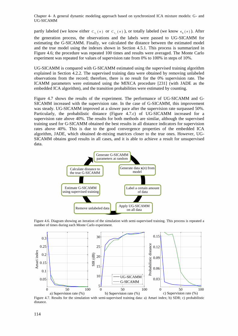
Chapter 4- A general dynamic modeling approach based on synchronized ICA mixture models: G- and
UG-SICAMM
114
partly labeled (we know either 1
kC n or
2k
C n ), or totally labeled (we know nk
c ). After
the generation process, the observations and the labels were passed to UG-SICAMM for
estimating the G-SICAMM. Finally, we calculated the distance between the estimated model
and the true model using the indexes shown in Section 4.5.1. This process is summarized in
Figure 4.6; the procedure was repeated 100 times and results were averaged. The Monte Carlo
experiment was repeated for values of supervision rate from 0% to 100% in steps of 10%.
UG-SICAMM is compared with G-SICAMM estimated using the supervised training algorithm
explained in Section 4.2.2. The supervised training data were obtained by removing unlabeled
observations from the record; therefore, there is no result for the 0% supervision rate. The
ICAMM parameters were estimated using the MIXCA procedure [231] (with JADE as the
embedded ICA algorithm), and the transition probabilities were estimated by counting.
Figure 4.7 shows the results of the experiment. The performance of UG-SICAMM and G-
SICAMM increased with the supervision rate. In the case of G-SICAMM, this improvement
was steady. UG-SICAMM improved at a slower pace after the supervision rate surpassed 50%.
Particularly, the probabilistic distance (Figure 4.7.c) of UG-SICAMM increased for a
supervision rate above 40%. The results for both methods are similar, although the supervised
training used for G-SICAMM obtained the best results in all distance indicators for supervision
rates above 40%. This is due to the good convergence properties of the embedded ICA
algorithm, JADE, which obtained de-mixing matrices closer to the true ones. However, UG-
SICAMM obtains good results in all cases, and it is able to achieve a result for unsupervised
data.
Figure 4.6. Diagram showing an iteration of the simulation with semi-supervised training. This process is repeated a
number of times during each Monte Carlo experiment.
Figure 4.7. Results for the simulation with semi-supervised training data: a) Amari index; b) SDR; c) probabilistic
distance.
Generate G-SICAMM parameters at random
Generate data x(n) from model
Label a certain amount of data
Apply UG-SICAMM on all dataRemove unlabeled data
Estimate G-SICAMM using supervised training
Calculate distance to the true G-SICAMM
0 50 100
0.05
0.1
0.15
0.2
0.25
0.3
a) Supervision rate (%)
Am
ari
in
dex
0 50 1005
10
15
20
25
30
b) Supervision rate (%)
SIR
(d
B)
0 50 100
0.03
0.06
0.09
0.12
0.15
c) Supervision rate (%)
Pro
bab
ilis
tic d
ista
nce
UG-SICAMM
G-SICAMM
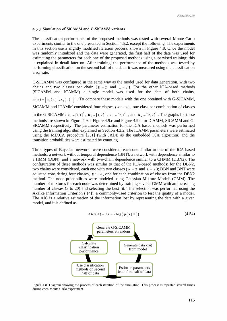
Simulations
115
4.5.3. Simulation of SICAMM and G-SICAMM variants
The classification performance of the proposed methods was tested with several Monte Carlo
experiments similar to the one presented in Section 4.5.2, except the following. The experiments
in this section use a slightly modified iteration process, shown in Figure 4.8. Once the model
was randomly initialized and the data were generated, the first half of the data was used for
estimating the parameters for each one of the proposed methods using supervised training; this
is explained in detail later on. After training, the performance of the methods was tested by
performing classification on the second half of the data; it was measured using the classification
error rate.
G-SICAMM was configured in the same way as the model used for data generation, with two
chains and two classes per chain ( 2K and 2L ). For the other ICA-based methods
(SICAMM and ICAMM) a single model was used for the data of both chains,
1 2,
TT T
n n n
x x x . To compare these models with the one obtained with G-SICAMM,
SICAMM and ICAMM considered four classes ' 4K , one class per combination of classes
in the G-SICAMM: 11,1
T
k , 21, 2
T
k , 32,1
T
k , and 42, 2
T
k . The graphs for these
methods are shown in Figure 4.9.a, Figure 4.9.c and Figure 4.9.e for ICAMM, SICAMM and G-
SICAMM respectively. The parameter estimation for the ICA-based methods was performed
using the training algorithm explained in Section 4.2.2. The ICAMM parameters were estimated
using the MIXCA procedure [231] (with JADE as the embedded ICA algorithm) and the
transition probabilities were estimated by counting.
Three types of Bayesian networks were considered, each one similar to one of the ICA-based
methods: a network without temporal dependence (BNT); a network with dependence similar to
a HMM (DBN); and a network with two-chain dependence similar to a CHMM (DBN2). The
configuration of these methods was similar to that of the ICA-based methods: for the DBN2,
two chains were considered, each one with two classes ( 2K and 2L ); DBN and BNT were
adjusted considering four classes, ' 4K , one for each combination of classes from the DBN2
method. The node probabilities were modeled using Gaussian Mixture Models (GMM). The
number of mixtures for each node was determined by training several GMM with an increasing
number of classes (3 to 20) and selecting the best fit. This selection was performed using the
Akaike Information Criterion ( [4]), a commonly-used criterion to test the quality of a model.
The AIC is a relative estimation of the information lost by representing the data with a given
model, and it is defined as
( ) 2 2 log |A IC k p x (4.54)
Figure 4.8. Diagram showing the process of each iteration of the simulation. This process is repeated several times
during each Monte Carlo experiment.
Generate G-SICAMM parameters at random
Generate data x(n) from model
Estimate parameters from first half of data
Use classification methods on second
half of data
Calculate classification performance
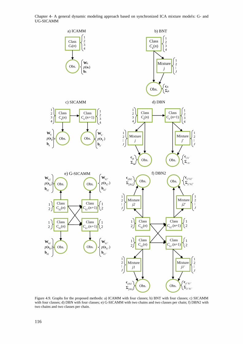
Chapter 4- A general dynamic modeling approach based on synchronized ICA mixture models: G- and
UG-SICAMM
116
Figure 4.9. Graphs for the proposed methods: a) ICAMM with four classes; b) BNT with four classes; c) SICAMM
with four classes; d) DBN with four classes; e) G-SICAMM with two chains and two classes per chain; f) DBN2 with
two chains and two classes per chain.
a) ICAMM
Class
Ck(n)
Obs.
1
2
3 4
Wk
p(sk)
bk
b) BNT
Class C
k(n)
1 2 3 4
Obs. cjk Σjk
Mixture j
1 2 ⁞ J
c) SICAMM
Class
Ck(n)
Obs.
Wk
p(sk)
bk
Class
Ck’
(n+1)
Obs.
1
2 3
4
Wk’
p(sk’
)
bk’
1 2
3
4
d) DBN
Class
Ck’
(n+1)
1 2 3 4
Obs. c
j’k’
Σj’k’
Mixture
j'
1 2 ⁞ J
Class
Ck(n)
Obs. cjk
Σjk
Mixture
j
1 2
3
4
1 2
⁞
J
e) G-SICAMM
Class
Ck1
(n)
Obs.
Wk1
p(sk1
) b
k1
Class
Ck1’
(n+1)
Obs.
1 2
Wk1’
p(s
k1’)
bk1’
1 2
Class
Ck2
(n)
Obs.
Wk2
p(sk2
) b
k2
Class
Ck2’
(n+1)
Obs.
Wk2’
p(s
k2’)
bk2’
1 2
1 2
f) DBN2
Class
Ck1’
(n+1)
Obs. c
j1’k1’
Σj1’k1’
Mixture
j1'
1
2 ⁞
J
Class
Ck1
(n)
Obs. c
j1k1
Σj1k1
Mixture
j1
1
2 ⁞
J
Class
Ck2’
(n+1)
Obs. c
j2’k2’
Σj2’k2’
Mixture
j2'
1
2
⁞
J
Class
Ck2
(n)
Obs. c
j2k2
Σj2k2
Mixture
j2
1
2
⁞
J
1
2
1
2
1
2
1
2
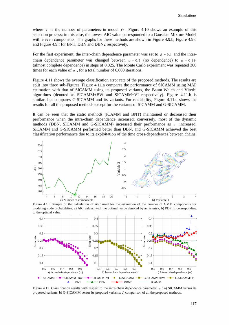
Simulations
117
where k is the number of parameters in model . Figure 4.10 shows an example of this
selection process; in this case, the lowest AIC value corresponded to a Gaussian Mixture Model
with eleven components. The graphs for these methods are shown in Figure 4.9.b, Figure 4.9.d
and Figure 4.9.f for BNT, DBN and DBN2 respectively.
For the first experiment, the inter-chain dependence parameter was set to 0 .1 and the intra-
chain dependence parameter was changed between 0 .5 (no dependence) to 0 .99
(almost complete dependence) in steps of 0.025. The Monte Carlo experiment was repeated 300
times for each value of , for a total number of 6,000 iterations.
Figure 4.11 shows the average classification error rate of the proposed methods. The results are
split into three sub-Figures. Figure 4.11.a compares the performance of SICAMM using MAP
estimation with that of SICAMM using its proposed variants, the Baum-Welch and Viterbi
algorithms (denoted as SICAMM+BW and SICAMM+VI respectively). Figure 4.11.b is
similar, but compares G-SICAMM and its variants. For readability, Figure 4.11.c shows the
results for all the proposed methods except for the variants of SICAMM and G-SICAMM.
It can be seen that the static methods (ICAMM and BNT) maintained or decreased their
performance when the intra-chain dependence increased; conversely, most of the dynamic
methods (DBN, SICAMM and G-SICAMM) increased their performance as increased.
SICAMM and G-SICAMM performed better than DBN, and G-SICAMM achieved the best
classification performance due to its exploitation of the time cross-dependences between chains.
Figure 4.10. Sample of the calculation of AIC used for the estimation of the number of GMM components for
modeling node probabilities: a) AIC values, with the optimal value denoted by an asterisk; b) PDF fit corresponding
to the optimal value.
Figure 4.11. Classification results with respect to the intra-chain dependence parameter, : a) SICAMM versus its
proposed variants; b) G-SICAMM versus its proposed variants; c) comparison of all the proposed methods.
4 6 8 10 12 14 16 18 20
480
485
490
495
500
505
510
515
520
a) Number of components
AIC
-2 -1 0 1 2 3 4-1
-0.5
0
0.5
1
1.5
2
2.5
3
b) Variable 1
Var
iable
2
0.5 0.6 0.7 0.8 0.9
0.1
0.15
0.2
0.25
0.3
0.35
0.4
a) Intra-chain dependence ()
Err
or
rate
0.5 0.6 0.7 0.8 0.9
0.1
0.15
0.2
0.25
0.3
0.35
0.4
b) Intra-chain dependence ()
Err
or
rate
0.5 0.6 0.7 0.8 0.9
0.1
0.15
0.2
0.25
0.3
0.35
0.4
c) Intra-chain dependence ()
Err
or
rate
BNT DBN DBN2 ICAMM
SICAMM SICAMM+BW SICAMM+VI G-SICAMM G-SICAMM+BW G-SICAMM+VI
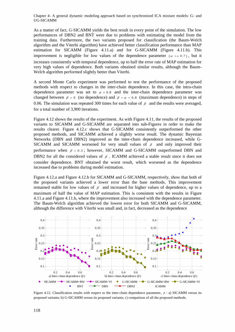
Chapter 4- A general dynamic modeling approach based on synchronized ICA mixture models: G- and
UG-SICAMM
118
As a matter of fact, G-SICAMM yields the best result in every point of the simulation. The low
performances of DBN2 and BNT were due to problems with estimating the model from the
training data. Furthermore, the two variants proposed for classification (the Baum-Welch
algorithm and the Viterbi algorithm) have achieved better classification performance than MAP
estimation for SICAMM (Figure 4.11.a) and for G-SICAMM (Figure 4.11.b). This
improvement is negligible for low values of the dependence parameter 0 .7 , but it
increases consistently with temporal dependence, up to half the error rate of MAP estimation for
very high values of dependence. Both variants obtained similar results, although the Baum-
Welch algorithm performed slightly better than Viterbi.
A second Monte Carlo experiment was performed to test the performance of the proposed
methods with respect to changes in the inter-chain dependence. In this case, the intra-chain
dependence parameter was set to 0 .8 and the inter-chain dependence parameter was
changed between 0 (no dependence) and 0 .8 (maximum dependence) in steps of
0.06. The simulation was repeated 300 times for each value of and the results were averaged,
for a total number of 3,900 iterations.
Figure 4.12 shows the results of the experiment. As with Figure 4.11, the results of the proposed
variants to SICAMM and G-SICAMM are separated into sub-Figures in order to make the
results clearer. Figure 4.12.c shows that G-SICAMM consistently outperformed the other
proposed methods, and SICAMM achieved a slightly worse result. The dynamic Bayesian
Networks (DBN and DBN2) improved as the inter-chain dependence increased, while G-
SICAMM and SICAMM worsened for very small values of and only improved their
performance when 0 .3 ; however, SICAMM and G-SICAMM outperformed DBN and
DBN2 for all the considered values of . ICAMM achieved a stable result since it does not
consider dependence. BNT obtained the worst result, which worsened as the dependence
increased due to problems during model estimation.
Figure 4.12.a and Figure 4.12.b for SICAMM and G-SICAMM, respectively, show that both of
the proposed variants achieved a lower error than the base methods. This improvement
remained stable for low values of and increased for higher values of dependence, up to a
maximum of half the value of MAP estimation. This is consistent with the results in Figure
4.11.a and Figure 4.11.b, where the improvement also increased with the dependence parameter.
The Baum-Welch algorithm achieved the lowest error for both SICAMM and G-SICAMM,
although the difference with Viterbi was small and, in fact, decreased as the dependence
Figure 4.12. Classification results with respect to the inter-chain dependence parameter, : a) SICAMM versus its
proposed variants; b) G-SICAMM versus its proposed variants; c) comparison of all the proposed methods.
0.2 0.4 0.6
0.1
0.15
0.2
0.25
0.3
0.35
0.4
a) Inter-chain dependence ()
Err
or
rate
0.2 0.4 0.6
0.1
0.15
0.2
0.25
0.3
0.35
0.4
b) Inter-chain dependence ()
Err
or
rate
0.2 0.4 0.6
0.1
0.15
0.2
0.25
0.3
0.35
0.4
c) Inter-chain dependence ()
Err
or
rate
BNT DBN DBN2 ICAMM
SICAMM SICAMM+BW SICAMM+VI G-SICAMM G-SICAMM+BW G-SICAMM+VI
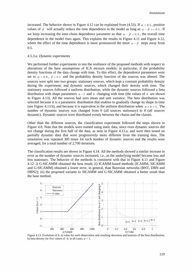
Simulations
119
increased. The behavior shown in Figure 4.12 can be explained from (4.53). If 0 .5 , positive
values of will actually reduce the time dependence in the model as long as 0 .5 . If
we keep increasing the inter-chain dependence parameter so that 0 .5 , the overall time
dependence in the model rises again. This explains the results in Figure 4.11 and Figure 4.12,
where the effect of the time dependence is more pronounced the more steps away from
0.5.
4.5.3.a. Dynamic experiments
We performed further experiments to test the resilience of the proposed methods with respect to
alterations of the base assumptions of ICA mixture models: in particular, if the probability
density functions of the data change with time. To this effect, the dependence parameters were
set to 0 .8 , 0 .1 and the probability density function of the sources was altered. The
sources were split into two groups: stationary sources, which kept a constant probability density
during the experiment; and dynamic sources, which changed their density with time. The
stationary sources followed a uniform distribution, while the dynamic sources followed a beta
distribution with shape parameters 1a and b changing with time (the values of b are shown
in Figure 4.13). All the sources had zero mean and unit variance. The beta distribution was
selected because it is a parametric distribution that enables to gradually change its shape in time
(see Figure 4.13.b), and because it is equivalent to the uniform distribution when 1a b . The
number of dynamic sources was changed from 0 (all sources stationary) to 8 (all sources
dynamic). Dynamic sources were distributed evenly between the chains and the classes.
Other than the different sources, the classification experiment followed the steps shown in
Figure 4.8. Note that the models were trained using static data, since even dynamic sources did
not change during the first half of the data, as seen in Figure 4.13.a, and were then tested on
partially dynamic data that were progressively more different from the training data. The
simulation was repeated 300 times for each number of dynamic sources and the results were
averaged, for a total number of 2,700 iterations.
The classification results are shown in Figure 4.14. All the methods showed a similar increase in
error as the number of dynamic sources increased, i.e., as the underlying model became less and
less stationary. The behavior of the methods is consistent with that in Figure 4.11 and Figure
4.12: i) G-SICAMM obtained the best result; ii) ICAMM-based methods (ICAMM, SICAMM
and G-SICAMM) obtained a lower error, in general, than Bayesian networks (BNT, DBN and
DBN2); iii) the proposed variants to SICAMM and G-SICAMM obtained a better result than
the base method.
Figure 4.13. Evolution of b: a) value for each observation and resulting skewness and kurtosis of the beta distribution;
b) beta density for five values of b; in all cases, a = 1.
200 400 600 800 1000
-1
0
1
2
3
4
5
a) Sample
Val
ues
fo
r a
= 1
0 0.2 0.4 0.6 0.8 1
0
1
2
3
4
5
b=5 b=3 b=2 b=1.5 b=1
b) Value
Bet
a d
istr
ibu
tio
n f
or
a=
1 a
nd
ch
ang
ing
b
Kurtosis
Skewness
b value
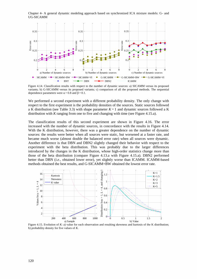
Chapter 4- A general dynamic modeling approach based on synchronized ICA mixture models: G- and
UG-SICAMM
120
Figure 4.14. Classification results with respect to the number of dynamic sources: a) SICAMM versus its proposed
variants; b) G-SICAMM versus its proposed variants; c) comparison of all the proposed methods. The sequential
dependence parameters were α = 0.8 and β = 0.1.
We performed a second experiment with a different probability density. The only change with
respect to the first experiment is the probability densities of the sources. Static sources followed
a K distribution (see Table 3.3) with shape parameter K = 1 and dynamic sources followed a K
distribution with K ranging from one to five and changing with time (see Figure 4.15.a).
The classification results of this second experiment are shown in Figure 4.16. The error
increased with the number of dynamic sources, in concordance with the results in Figure 4.14.
With the K distribution, however, there was a greater dependence on the number of dynamic
sources: the results were better when all sources were static, but worsened at a faster rate, and
became much worse (almost double the balanced error rate) when all sources were dynamic.
Another difference is that DBN and DBN2 slightly changed their behavior with respect to the
experiment with the beta distribution. This was probably due to the larger differences
introduced by the changes in the K distribution, whose high-order statistics change more than
those of the beta distribution (compare Figure 4.13.a with Figure 4.15.a). DBN2 performed
better than DBN (i.e., obtained lower error), yet slightly worse than ICAMM. ICAMM-based
methods obtained the best results, and G-SICAMM+BW obtained the lowest error rate.
Figure 4.15. Evolution of K: a) value for each observation and resulting skewness and kurtosis of the K distribution;
b) probability density for five values of K.
0 2 4 6 8
0.2
0.25
0.3
0.35
a) Number of dynamic sources
Err
or
rate
0 2 4 6 8
0.2
0.25
0.3
0.35
b) Number of dynamic sources
Err
or
rate
0 2 4 6 8
0.2
0.25
0.3
0.35
c) Number of dynamic sources
Err
or
rate
BNT DBN DBN2 ICAMM
SICAMM SICAMM+BW SICAMM+VI G-SICAMM G-SICAMM+BW G-SICAMM+VI
200 400 600 800 1000
2
4
6
8
10
12
14
16
a) Sample
Val
ues
fo
r
= 1
, L
= 4
0 0.5 1 1.5 20
0.2
0.4
0.6
0.8
1
1.2
b) Value
Dis
trib
uti
on
fo
r =
1,
L =
4,
and
ch
ang
ing
K
Kurtosis
Skewness
K value
K=1
K=1.5
K=2
K=3
K=5
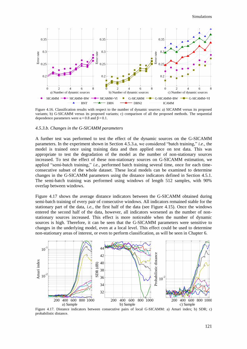
Simulations
121
Figure 4.16. Classification results with respect to the number of dynamic sources: a) SICAMM versus its proposed
variants; b) G-SICAMM versus its proposed variants; c) comparison of all the proposed methods. The sequential
dependence parameters were α = 0.8 and β = 0.1.
4.5.3.b. Changes in the G-SICAMM parameters
A further test was performed to test the effect of the dynamic sources on the G-SICAMM
parameters. In the experiment shown in Section 4.5.3.a, we considered “batch training,” i.e., the
model is trained once using training data and then applied once on test data. This was
appropriate to test the degradation of the model as the number of non-stationary sources
increased. To test the effect of these non-stationary sources on G-SICAMM estimation, we
applied “semi-batch training,” i.e., performed batch training several time, once for each time-
consecutive subset of the whole dataset. These local models can be examined to determine
changes in the G-SICAMM parameters using the distance indicators defined in Section 4.5.1.
The semi-batch training was performed using windows of length 512 samples, with 90%
overlap between windows.
Figure 4.17 shows the average distance indicators between the G-SICAMM obtained during
semi-batch training of every pair of consecutive windows. All indicators remained stable for the
stationary part of the data, i.e., the first half of the data (see Figure 4.15). Once the windows
entered the second half of the data, however, all indicators worsened as the number of non-
stationary sources increased. This effect is more noticeable when the number of dynamic
sources is high. Therefore, it can be seen that the G-SICAMM parameters were sensitive to
changes in the underlying model, even at a local level. This effect could be used to determine
non-stationary areas of interest, or even to perform classification, as will be seen in Chapter 6.
Figure 4.17. Distance indicators between consecutive pairs of local G-SICAMM: a) Amari index; b) SDR; c)
probabilistic distance.
0 2 4 6 8
0.2
0.25
0.3
0.35
a) Number of dynamic sources
Err
or
rate
0 2 4 6 8
0.2
0.25
0.3
0.35
b) Number of dynamic sources
Err
or
rate
0 2 4 6 8
0.2
0.25
0.3
0.35
c) Number of dynamic sources
Err
or
rate
BNT DBN DBN2 ICAMM
SICAMM SICAMM+BW SICAMM+VI G-SICAMM G-SICAMM+BW G-SICAMM+VI
200 400 600 800 1000
10-2
10-1
a) Sample
Am
ari
in
dex
0
12
34
5
67
8
200 400 600 800 1000
32
34
36
38
40
42
44
b) Sample
SD
R (
dB
)
0
1234
5
6
7
8200 400 600 800 1000
10-2
c) Sample
Pro
bab
ilis
tic d
ista
nce
0
12
3
4
5
6
7
8

Chapter 4- A general dynamic modeling approach based on synchronized ICA mixture models: G- and
UG-SICAMM
122
4.6. Conclusions
This chapter has introduced two extensions of Sequential ICAMM, a dynamic model based on
ICA mixture modeling that takes into account the temporal dependences in the data that the
basic ICAMM does not consider [230]. The first one of these extensions is based on the
similarities between SICAMM and Hidden Markov Models. Because of these similarities, when
SICAMM is used for classification, the result can be improved by considering two classical
classification algorithms, Baum-Welch and Viterbi. The Baum-Welch algorithm performs a
forward-backward estimation of the class probabilities while making use of all available data,
while the Viterbi algorithm is a classical decoding algorithm that can find the most likely
sequence of classes in the data without performing an exhaustive search. The second extension
of SICAMM is a generalization of the concept of SICAMM to work with any number of
parallel chains which are inter-related, each one a SICAMM on its own. This extension has been
named Generalized SICAMM (G-SICAMM). Such a method can be used to work
simultaneously with several datasets in parallel, or to split the data into multiple sub-chains.
Furthermore, both the Baum-Welch and the Viterbi algorithms can be used to improve the
results of G-SICAMM as well, combining both proposed extensions to SICAMM.
If labeled data are available for training, the estimation of the time dependence parameters can
be performed separately from the estimation of the ICAMM parameters, both for SICAMM and
G-SICAMM. In that case, the parameters can be estimated using known methods. However, if
some training data is unlabeled (i.e., we perform semi-supervised or unsupervised training), all
of the G-SICAMM parameters have to be estimated simultaneously. This chapter presents an
algorithm for semi-supervised or unsupervised training of SICAMM and G-SICAMM, which
we have named UG-SICAMM.
The performance of UG-SICAMM was tested by assessing the distance between the estimated
model and the true model using a Monte Carlo experiment with an increasing number of labeled
data, from unsupervised (all of the data are unlabeled) to fully-supervised (all of the data are
labeled) training. To this effect, three distance indicators were proposed: i) the Amari index,
which calculates the distance between de-mixing matrices; ii) the signal-to-interference ratio,
which measures the similarity between the recovered sources and the true sources; iii) the
probabilistic distance, which determines the difference between the dynamic behavior of two
given models. The results show that the distance to the true model decreased as the amount of
supervised data increased; although this improvement was faster for low supervision rates than
it was for high supervision rates. Out of the considered indicators, the SIR and Amari indices
were the ones that improved the most when the amount of labeled data increased, while the
probabilistic distance did not improve for high amounts of supervision.
The performance of SICAMM and G-SICAMM was tested by performing classification on
several sets of simulated data, and compared with that of Bayesian Networks (BNT) and
Dynamic Bayesian Networks (DBN and DBN2). This study was performed using several Monte
Carlo experiments, considering changes in the time dependence of the simulated data; this
dependence was modeled with two values, the intra-chain dependence parameter and the
inter-chain dependence parameter . The results show that the dynamic methods (DBN,
DBN2, SICAMM and G-SICAMM) performed better than the static ones (BNT and ICAMM)
because they exploit the time dependences between observations. The ICA-based methods
always obtained a better classification than the similar Bayesian-network-based methods, i.e.,
ICAMM performed better than BNT, and SICAMM and G-SICAMM performed better than
DBN and DBN2. Furthermore, G-SICAMM always obtained the best result because it was able
to exploit more time dependences than the other methods. Furthermore, it has been shown that
SICAMM and G-SICAMM improve their results if the classification is performed using the
Baum-Welch or the Viterbi algorithms. The improvement was negligible for small dependence
values, but it increased with the dependence in the data up to a maximum result of half the error

Conclusions
123
of the base methods. The behavior of the proposed methods was the same for both types of
dependence, although it was more pronounced for changes in the inter-chain dependence.
Finally, we tested the behavior of the proposed methods when the basic ICAMM assumptions
could not be met; particularly, when the probability density of the sources was not stationary,
but rather changed over time. This was done using two Monte Carlo experiments with an
increasing number of non-stationary sources, i.e., sources that changed in distribution after
training. In the first experiment, the sources were originally uniformly distributed, but then
changed according to a beta distribution. In the second experiment, the sources were K-
distributed and the K parameter changed with time. In both cases, all the proposed methods
worsened at a similar rate as the number of non-stationary sources increased. The performance
of the methods was consistent with that of the previous simulations, and G-SICAMM+BW
obtained the best result, followed by G-SICAMM+VI and SICAMM+BW. It was found that the
performance on the K-distributed data was more affected by the non-stationarity than the
performance on beta-distributed data. Furthermore, it was shown that the G-SICAMM
parameters are sensitive to these changes in the model. Local estimations of the G-SICAMM
were found to be similar if the data were stationary, and became more and more different as the
data became more dynamic.
The results in this chapter show the potential of the proposed G-SICAMM procedure. The
classification performance was the best out of the considered methods, and it was further
improved by the use of the Baum-Welch algorithm. The parameters of the model can be
obtained from semi-labeled or unlabeled data, which increases the range of possible applications
for the procedure. Furthermore, although it was not considered in this chapter, the G-SICAMM
parameters can be interpreted on their own and provide a structured result which can model the
local behavior of the data without compromising its generalization capabilities.

125
Application of PREDICAMM to non-destructive testing and EEG signal processing applications
5


127
- Application of PREDICAMM to non-destructive testing and EEG signal processing applications
This chapter presents three applications of signal prediction using the proposed PREDICAMM
and E-ICAMM methods explained in Section 3.1 and 3.2, respectively. The results of
PREDICAMM are compared with those of Kriging, Wiener structures, and spherical splines
(also explained in Section 3.3). The proposed methods were tested on one set of simulated
ground-penetrating radar data and three applications on real data: recovery of GPR data of real
scale replicas of historical walls, reconstruction of data from a seismic survey, and interpolation
of missing electroencephalographic data from a memory task.
The first application is based on non-destructive testing (NDT) signals from a ground-
penetrating radar survey on real scale replicas of historical walls. In NDT applications, the
signals are usually spatially distributed, forming two-dimensional sets of data or B-Scans. As
explained in Chapter 3, PREDICAMM and E-ICAMM are able to perform prediction in data of
any shape, even spatial data, depending on how the ICAMM is calculated. However, in this
work, spatial data were preprocessed to be converted into time-distributed signals. This is a
common preprocessing step in image processing applications, including several methods based
on ICA such as Topographical ICA [111] and hierarchical ICA mixture models [240].
The second application performs prediction on data from a reflection seismology survey, where
the subsurface is explored by a careful study of reflected seismic waves. The proposed methods
were tested on a set of true seismic data from an underwater exploration.
The third application consists of the reconstruction of artifacted or missing data from an
electroencephalogram, a record of the electrical activity of the brain taken on the scalp.
PREDICAMM and E-ICAMM were applied to EEG data captured on subjects that were
performing the Sternberg memory task, a classical procedure for evaluation of the short-term
memory function. Prediction performance was estimated by means of a Monte Carlo experiment
with a growing number of missing channels. The proposed methods were compared with
spherical splines, a commonly-used interpolation method for EEG data.
In all three applications, the performance of the proposed methods will be quantified using the
four error indicators introduced in Section 3.4.2. These indicators are: i) the signal-to-

Chapter 5- Application of PREDICAMM to non-destructive testing and EEG signal processing
applications
128
interference ratio, which quantifies the average squared error in the prediction; ii) the Kullback-
Leibler divergence, a measure of the distance between the probability density function of the
original data and of the PDF of the reconstructed data; iii) the cross-correlation between the
original data and the reconstructed data, an indicator of the temporal similarity of both sets of
data; and iv) the mean structural similarity, a similarity measure between two images that
compares their structures.
5.1. Non-destructive testing simulations
Non-destructive testing is a set of techniques that allow the structure of a material to be
analyzed without damaging it. They are usually used to characterize a material or to test its
integrity in cases where there is no option to sample or affect the material under test; this can
happen for a number of reasons, mainly:
The material under test must remain undamaged and it cannot be duplicated, e.g., the
testing of archaeological objects [229,62] or historical buildings [99,212].
The material under test is unreachable and no sample can be obtained, e.g., seismic
exploration of underground environments [177,105] or remote sensing [71].
There are many objects under test and taking samples out of every single one of them is
unfeasible, e.g., quality testing of products before they leave the production chain [205].
The material is hazardous, e.g., landmine detection [90].
When any element of a NDT system fails, some information can be lost, resulting in missing
data (also known as missing traces). The reconstruction of this information from the rest of
captured data is not a straightforward work; in fact, this reconstruction is an ill-posed problem.
Field studies are particularly exposed to this kind of problem, since they usually involve an
amount of sensors spread over a hostile area; it is quite usual that several traces are lost or mis-
captured for any number of reasons. Furthermore, reconstruction methods can be used even if
there is no actual data loss. For instance, they can be used to interpolate data and achieve the
same resolution with a lower number of sensors (e.g., by considering that every other trace is
missing).
The reconstruction scenario is well-known in the literature and several algorithms have been
proposed to deal with it. Nevertheless, data reconstruction remains an interesting research topic
(given its difficulty) and it is the subject of current research. Most of the algorithms proposed
for this task make use of low-order statistical properties of the signals involved, e.g., linear
predictors [163,116].
In particular, in this thesis, we will consider NDT signals in the areas of ground penetrating
radar and seismic exploration surveys. There are only a few examples of the application of ICA
and ICAMM to problems related with seismic and GPR signal processing. The motivation of
using ICAMM to these application areas is the degrees of freedom provided by ICAMM, which
allow for linear local projections that can be adapted to partial segments of a data set while
maintaining generalization (capability for nonlinear modeling) given the mixture of several
ICAs. Furthermore, the normal method to represent the results in seismic exploration and GPR
is using images (B-Scans) called seismograms and radargrams, respectively. ICA has been
extensively applied to image processing in problems such as filtering [19], segmentation [152],
face recognition [135,16], and processing of biomedical images [168,255]. Briefly, images
patches values taken from the pixels of the image are considered as variables for ICA
processing, and the estimated basis functions (mixing matrix) and sources are used for image
application. Thus, we will process radargrams and seismograms as images applying the
proposed methods based on ICAMM explained in Chapter 3.
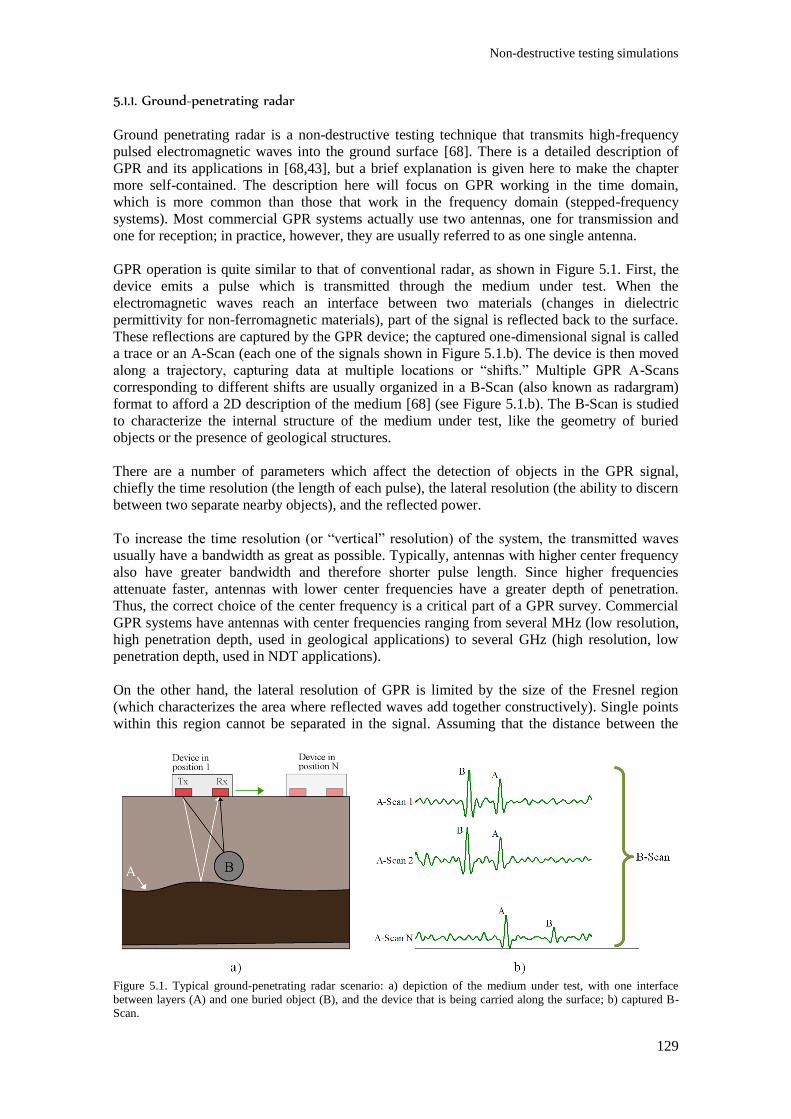
Non-destructive testing simulations
129
5.1.1. Ground-penetrating radar
Ground penetrating radar is a non-destructive testing technique that transmits high-frequency
pulsed electromagnetic waves into the ground surface [68]. There is a detailed description of
GPR and its applications in [68,43], but a brief explanation is given here to make the chapter
more self-contained. The description here will focus on GPR working in the time domain,
which is more common than those that work in the frequency domain (stepped-frequency
systems). Most commercial GPR systems actually use two antennas, one for transmission and
one for reception; in practice, however, they are usually referred to as one single antenna.
GPR operation is quite similar to that of conventional radar, as shown in Figure 5.1. First, the
device emits a pulse which is transmitted through the medium under test. When the
electromagnetic waves reach an interface between two materials (changes in dielectric
permittivity for non-ferromagnetic materials), part of the signal is reflected back to the surface.
These reflections are captured by the GPR device; the captured one-dimensional signal is called
a trace or an A-Scan (each one of the signals shown in Figure 5.1.b). The device is then moved
along a trajectory, capturing data at multiple locations or “shifts.” Multiple GPR A-Scans
corresponding to different shifts are usually organized in a B-Scan (also known as radargram)
format to afford a 2D description of the medium [68] (see Figure 5.1.b). The B-Scan is studied
to characterize the internal structure of the medium under test, like the geometry of buried
objects or the presence of geological structures.
There are a number of parameters which affect the detection of objects in the GPR signal,
chiefly the time resolution (the length of each pulse), the lateral resolution (the ability to discern
between two separate nearby objects), and the reflected power.
To increase the time resolution (or “vertical” resolution) of the system, the transmitted waves
usually have a bandwidth as great as possible. Typically, antennas with higher center frequency
also have greater bandwidth and therefore shorter pulse length. Since higher frequencies
attenuate faster, antennas with lower center frequencies have a greater depth of penetration.
Thus, the correct choice of the center frequency is a critical part of a GPR survey. Commercial
GPR systems have antennas with center frequencies ranging from several MHz (low resolution,
high penetration depth, used in geological applications) to several GHz (high resolution, low
penetration depth, used in NDT applications).
On the other hand, the lateral resolution of GPR is limited by the size of the Fresnel region
(which characterizes the area where reflected waves add together constructively). Single points
within this region cannot be separated in the signal. Assuming that the distance between the
Figure 5.1. Typical ground-penetrating radar scenario: a) depiction of the medium under test, with one interface
between layers (A) and one buried object (B), and the device that is being carried along the surface; b) captured B-
Scan.
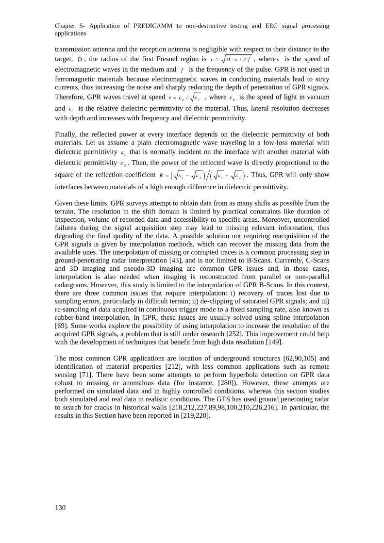
Chapter 5- Application of PREDICAMM to non-destructive testing and EEG signal processing
applications
130
transmission antenna and the reception antenna is negligible with respect to their distance to the
target, D , the radius of the first Fresnel region is / 2r D v f , where v is the speed of
electromagnetic waves in the medium and f is the frequency of the pulse. GPR is not used in
ferromagnetic materials because electromagnetic waves in conducting materials lead to stray
currents, thus increasing the noise and sharply reducing the depth of penetration of GPR signals.
Therefore, GPR waves travel at speed 0
/r
v c , where 0
c is the speed of light in vacuum
and r
is the relative dielectric permittivity of the material. Thus, lateral resolution decreases
with depth and increases with frequency and dielectric permittivity.
Finally, the reflected power at every interface depends on the dielectric permittivity of both
materials. Let us assume a plain electromagnetic wave traveling in a low-loss material with
dielectric permittivity 1
that is normally incident on the interface with another material with
dielectric permittivity 2
. Then, the power of the reflected wave is directly proportional to the
square of the reflection coefficient 1 2 1 2R . Thus, GPR will only show
interfaces between materials of a high enough difference in dielectric permittivity.
Given these limits, GPR surveys attempt to obtain data from as many shifts as possible from the
terrain. The resolution in the shift domain is limited by practical constraints like duration of
inspection, volume of recorded data and accessibility to specific areas. Moreover, uncontrolled
failures during the signal acquisition step may lead to missing relevant information, thus
degrading the final quality of the data. A possible solution not requiring reacquisition of the
GPR signals is given by interpolation methods, which can recover the missing data from the
available ones. The interpolation of missing or corrupted traces is a common processing step in
ground-penetrating radar interpretation [43], and is not limited to B-Scans. Currently, C-Scans
and 3D imaging and pseudo-3D imaging are common GPR issues and, in those cases,
interpolation is also needed when imaging is reconstructed from parallel or non-parallel
radargrams. However, this study is limited to the interpolation of GPR B-Scans. In this context,
there are three common issues that require interpolation: i) recovery of traces lost due to
sampling errors, particularly in difficult terrain; ii) de-clipping of saturated GPR signals; and iii)
re-sampling of data acquired in continuous trigger mode to a fixed sampling rate, also known as
rubber-band interpolation. In GPR, these issues are usually solved using spline interpolation
[69]. Some works explore the possibility of using interpolation to increase the resolution of the
acquired GPR signals, a problem that is still under research [252]. This improvement could help
with the development of techniques that benefit from high data resolution [149].
The most common GPR applications are location of underground structures [62,90,105] and
identification of material properties [212], with less common applications such as remote
sensing [71]. There have been some attempts to perform hyperbola detection on GPR data
robust to missing or anomalous data (for instance, [280]). However, these attempts are
performed on simulated data and in highly controlled conditions, whereas this section studies
both simulated and real data in realistic conditions. The GTS has used ground penetrating radar
to search for cracks in historical walls [218,212,227,89,98,100,210,226,216]. In particular, the
results in this Section have been reported in [219,220].
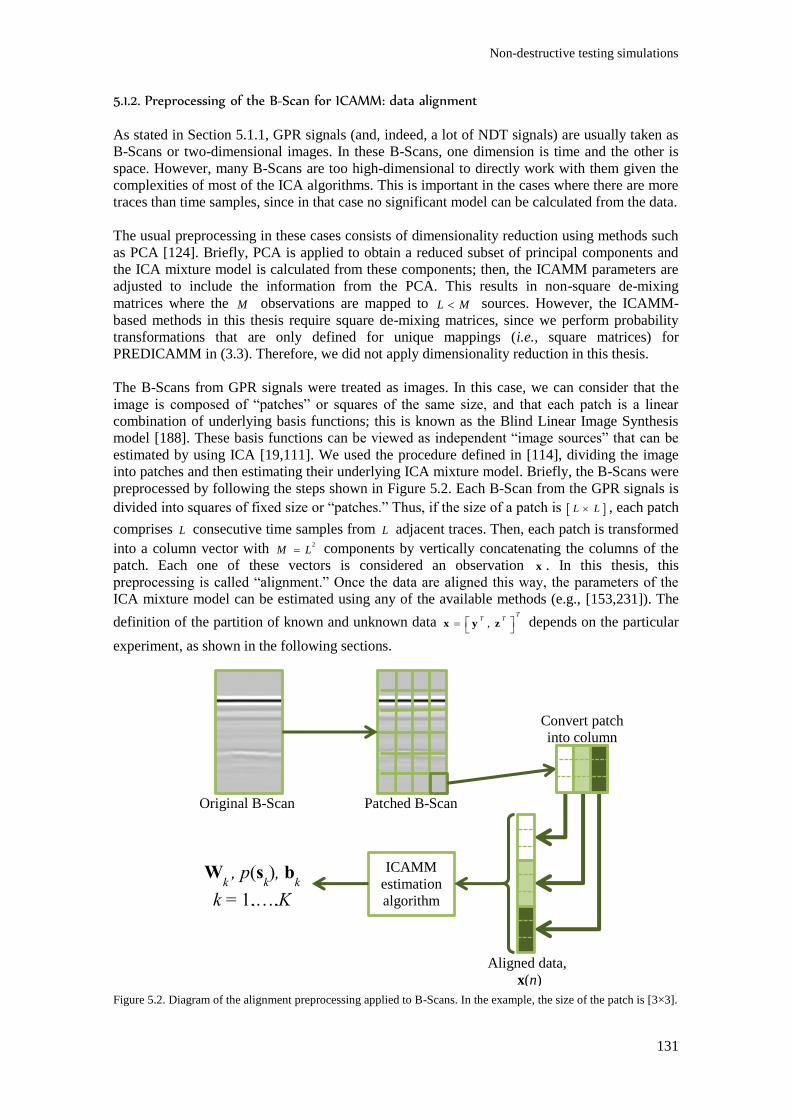
Non-destructive testing simulations
131
5.1.2. Preprocessing of the B-Scan for ICAMM: data alignment
As stated in Section 5.1.1, GPR signals (and, indeed, a lot of NDT signals) are usually taken as
B-Scans or two-dimensional images. In these B-Scans, one dimension is time and the other is
space. However, many B-Scans are too high-dimensional to directly work with them given the
complexities of most of the ICA algorithms. This is important in the cases where there are more
traces than time samples, since in that case no significant model can be calculated from the data.
The usual preprocessing in these cases consists of dimensionality reduction using methods such
as PCA [124]. Briefly, PCA is applied to obtain a reduced subset of principal components and
the ICA mixture model is calculated from these components; then, the ICAMM parameters are
adjusted to include the information from the PCA. This results in non-square de-mixing
matrices where the M observations are mapped to L M sources. However, the ICAMM-
based methods in this thesis require square de-mixing matrices, since we perform probability
transformations that are only defined for unique mappings (i.e., square matrices) for
PREDICAMM in (3.3). Therefore, we did not apply dimensionality reduction in this thesis.
The B-Scans from GPR signals were treated as images. In this case, we can consider that the
image is composed of “patches” or squares of the same size, and that each patch is a linear
combination of underlying basis functions; this is known as the Blind Linear Image Synthesis
model [188]. These basis functions can be viewed as independent “image sources” that can be
estimated by using ICA [19,111]. We used the procedure defined in [114], dividing the image
into patches and then estimating their underlying ICA mixture model. Briefly, the B-Scans were
preprocessed by following the steps shown in Figure 5.2. Each B-Scan from the GPR signals is
divided into squares of fixed size or “patches.” Thus, if the size of a patch is L L , each patch
comprises L consecutive time samples from L adjacent traces. Then, each patch is transformed
into a column vector with 2M L components by vertically concatenating the columns of the
patch. Each one of these vectors is considered an observation x . In this thesis, this
preprocessing is called “alignment.” Once the data are aligned this way, the parameters of the
ICA mixture model can be estimated using any of the available methods (e.g., [153,231]). The
definition of the partition of known and unknown data ,T
T T
x y z depends on the particular
experiment, as shown in the following sections.
Figure 5.2. Diagram of the alignment preprocessing applied to B-Scans. In the example, the size of the patch is [3×3].
ICAMM
estimation
algorithm
Wk , p(s
k), b
k
k = 1,…,K
Original B-Scan Patched B-Scan
Convert patch
into column
vector
Aligned data,
x(n)
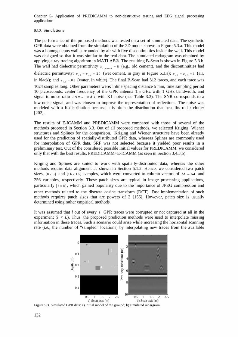
Chapter 5- Application of PREDICAMM to non-destructive testing and EEG signal processing
applications
132
5.1.3. Simulations
The performance of the proposed methods was tested on a set of simulated data. The synthetic
GPR data were obtained from the simulation of the 2D model shown in Figure 5.3.a. This model
was a homogeneous wall surrounded by air with five discontinuities inside the wall. This model
was designed so that it was similar to the real data. The simulated radargram was obtained by
applying a ray tracing algorithm in MATLAB®. The resulting B-Scan is shown in Figure 5.3.b.
The wall had dielectric permittivity ,
8r g ro u n d
(e.g., old cement), and the discontinuities had
dielectric permittivity: ,1 , 4
2 0r r
(wet cement, in gray in Figure 5.3.a); , 2 ,3
1r r
(air,
in black); and , 5
8 1r
(water, in white). The final B-Scan had 512 traces, and each trace was
1024 samples long. Other parameters were: inline spacing distance 5 mm, time sampling period
10 picoseconds, center frequency of the GPR antenna 1.5 GHz with 1 GHz bandwidth, and
signal-to-noise ratio 3 0 d BS N R with K1 noise (see Table 3.3). The SNR corresponds to a
low-noise signal, and was chosen to improve the representation of reflections. The noise was
modeled with a K-distribution because it is often the distribution that best fits radar clutter
[202].
The results of E-ICAMM and PREDICAMM were compared with those of several of the
methods proposed in Section 3.3. Out of all proposed methods, we selected Kriging, Wiener
structures and Splines for the comparison. Kriging and Wiener structures have been already
used for the prediction of spatially-distributed GPR data, whereas Splines are commonly used
for interpolation of GPR data. SRF was not selected because it yielded poor results in a
preliminary test. Out of the considered possible initial values for PREDICAMM, we considered
only that with the best results, PREDICAMM+E-ICAMM (as seen in Section 3.4.3.b).
Kriging and Splines are suited to work with spatially-distributed data, whereas the other
methods require data alignment as shown in Section 5.1.2. Hence, we considered two patch
sizes, [8 8 ] and [1 6 1 6 ] samples, which were converted to column vectors of 64M and
256 variables, respectively. These patch sizes are typical in image processing applications,
particularly 8 8 , which gained popularity due to the importance of JPEG compression and
other methods related to the discrete cosine transform (DCT). Fast implementation of such
methods requires patch sizes that are powers of 2 [156]. However, patch size is usually
determined using rather empirical methods.
It was assumed that l out of every L GPR traces were corrupted or not captured at all in the
experiment (l < L). Thus, the proposed prediction methods were used to interpolate missing
information in these traces. Such a scenario could arise while increasing the horizontal scanning
rate (i.e., the number of “sampled” locations) by interpolating new traces from the available
Figure 5.3. Simulated GPR data: a) initial model of the ground; b) simulated radargram.
Dep
th (
m)
a) Scan axis (m)
1
2
3
4 5
0.5 1 1.5 2 2.5
0
0.1
0.2
0.3
0.4
Tw
o-w
ay t
rav
elti
me
(ns)
b) Scan axis (m)0.5 1 1.5 2 2.5
2
4
6
8
10
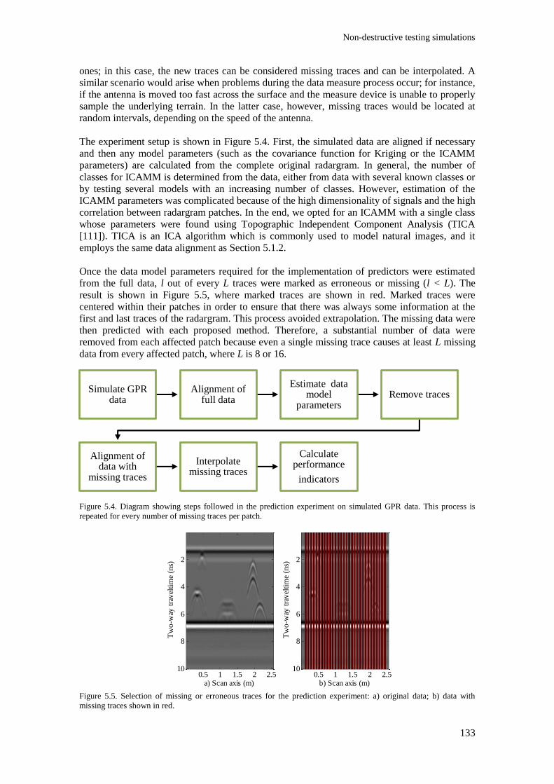
Non-destructive testing simulations
133
ones; in this case, the new traces can be considered missing traces and can be interpolated. A
similar scenario would arise when problems during the data measure process occur; for instance,
if the antenna is moved too fast across the surface and the measure device is unable to properly
sample the underlying terrain. In the latter case, however, missing traces would be located at
random intervals, depending on the speed of the antenna.
The experiment setup is shown in Figure 5.4. First, the simulated data are aligned if necessary
and then any model parameters (such as the covariance function for Kriging or the ICAMM
parameters) are calculated from the complete original radargram. In general, the number of
classes for ICAMM is determined from the data, either from data with several known classes or
by testing several models with an increasing number of classes. However, estimation of the
ICAMM parameters was complicated because of the high dimensionality of signals and the high
correlation between radargram patches. In the end, we opted for an ICAMM with a single class
whose parameters were found using Topographic Independent Component Analysis (TICA
[111]). TICA is an ICA algorithm which is commonly used to model natural images, and it
employs the same data alignment as Section 5.1.2.
Once the data model parameters required for the implementation of predictors were estimated
from the full data, l out of every L traces were marked as erroneous or missing (l < L). The
result is shown in Figure 5.5, where marked traces are shown in red. Marked traces were
centered within their patches in order to ensure that there was always some information at the
first and last traces of the radargram. This process avoided extrapolation. The missing data were
then predicted with each proposed method. Therefore, a substantial number of data were
removed from each affected patch because even a single missing trace causes at least L missing
data from every affected patch, where L is 8 or 16.
Figure 5.4. Diagram showing steps followed in the prediction experiment on simulated GPR data. This process is
repeated for every number of missing traces per patch.
Figure 5.5. Selection of missing or erroneous traces for the prediction experiment: a) original data; b) data with
missing traces shown in red.
Simulate GPR data
Alignment of full data
Estimate data model
parametersRemove traces
Alignment of data with
missing traces
Interpolate missing traces
Calculate performance
indicators
Tw
o-w
ay t
rav
elti
me
(ns)
a) Scan axis (m)0.5 1 1.5 2 2.5
2
4
6
8
10
Tw
o-w
ay t
rav
elti
me
(ns)
b) Scan axis (m)0.5 1 1.5 2 2.5
2
4
6
8
10
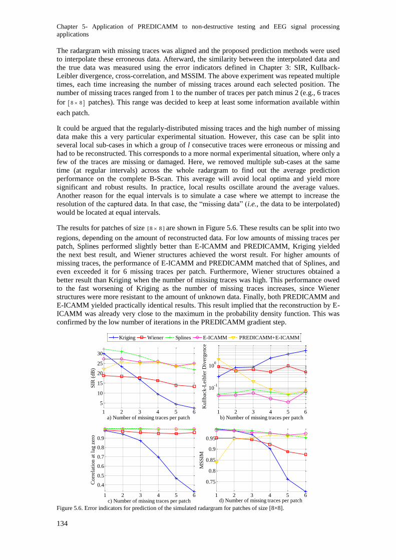
Chapter 5- Application of PREDICAMM to non-destructive testing and EEG signal processing
applications
134
The radargram with missing traces was aligned and the proposed prediction methods were used
to interpolate these erroneous data. Afterward, the similarity between the interpolated data and
the true data was measured using the error indicators defined in Chapter 3: SIR, Kullback-
Leibler divergence, cross-correlation, and MSSIM. The above experiment was repeated multiple
times, each time increasing the number of missing traces around each selected position. The
number of missing traces ranged from 1 to the number of traces per patch minus 2 (e.g., 6 traces
for 8 8 patches). This range was decided to keep at least some information available within
each patch.
It could be argued that the regularly-distributed missing traces and the high number of missing
data make this a very particular experimental situation. However, this case can be split into
several local sub-cases in which a group of l consecutive traces were erroneous or missing and
had to be reconstructed. This corresponds to a more normal experimental situation, where only a
few of the traces are missing or damaged. Here, we removed multiple sub-cases at the same
time (at regular intervals) across the whole radargram to find out the average prediction
performance on the complete B-Scan. This average will avoid local optima and yield more
significant and robust results. In practice, local results oscillate around the average values.
Another reason for the equal intervals is to simulate a case where we attempt to increase the
resolution of the captured data. In that case, the “missing data” (i.e., the data to be interpolated)
would be located at equal intervals.
The results for patches of size [8 8 ] are shown in Figure 5.6. These results can be split into two
regions, depending on the amount of reconstructed data. For low amounts of missing traces per
patch, Splines performed slightly better than E-ICAMM and PREDICAMM, Kriging yielded
the next best result, and Wiener structures achieved the worst result. For higher amounts of
missing traces, the performance of E-ICAMM and PREDICAMM matched that of Splines, and
even exceeded it for 6 missing traces per patch. Furthermore, Wiener structures obtained a
better result than Kriging when the number of missing traces was high. This performance owed
to the fast worsening of Kriging as the number of missing traces increases, since Wiener
structures were more resistant to the amount of unknown data. Finally, both PREDICAMM and
E-ICAMM yielded practically identical results. This result implied that the reconstruction by E-
ICAMM was already very close to the maximum in the probability density function. This was
confirmed by the low number of iterations in the PREDICAMM gradient step.
Figure 5.6. Error indicators for prediction of the simulated radargram for patches of size [8×8].
1 2 3 4 5 6
5
10
15
20
25
30
a) Number of missing traces per patch
SIR
(dB
)
1 2 3 4 5 6
10-1
100
b) Number of missing traces per patch
Kull
back-L
eib
ler
Div
erg
ence
1 2 3 4 5 6
0.4
0.5
0.6
0.7
0.8
0.9
c) Number of missing traces per patch
Corr
ela
tion a
t la
g z
ero
1 2 3 4 5 6
0.75
0.8
0.85
0.9
0.95
d) Number of missing traces per patch
MS
SIM
Kriging Wiener Splines E-ICAMM PREDICAMM+E-ICAMM
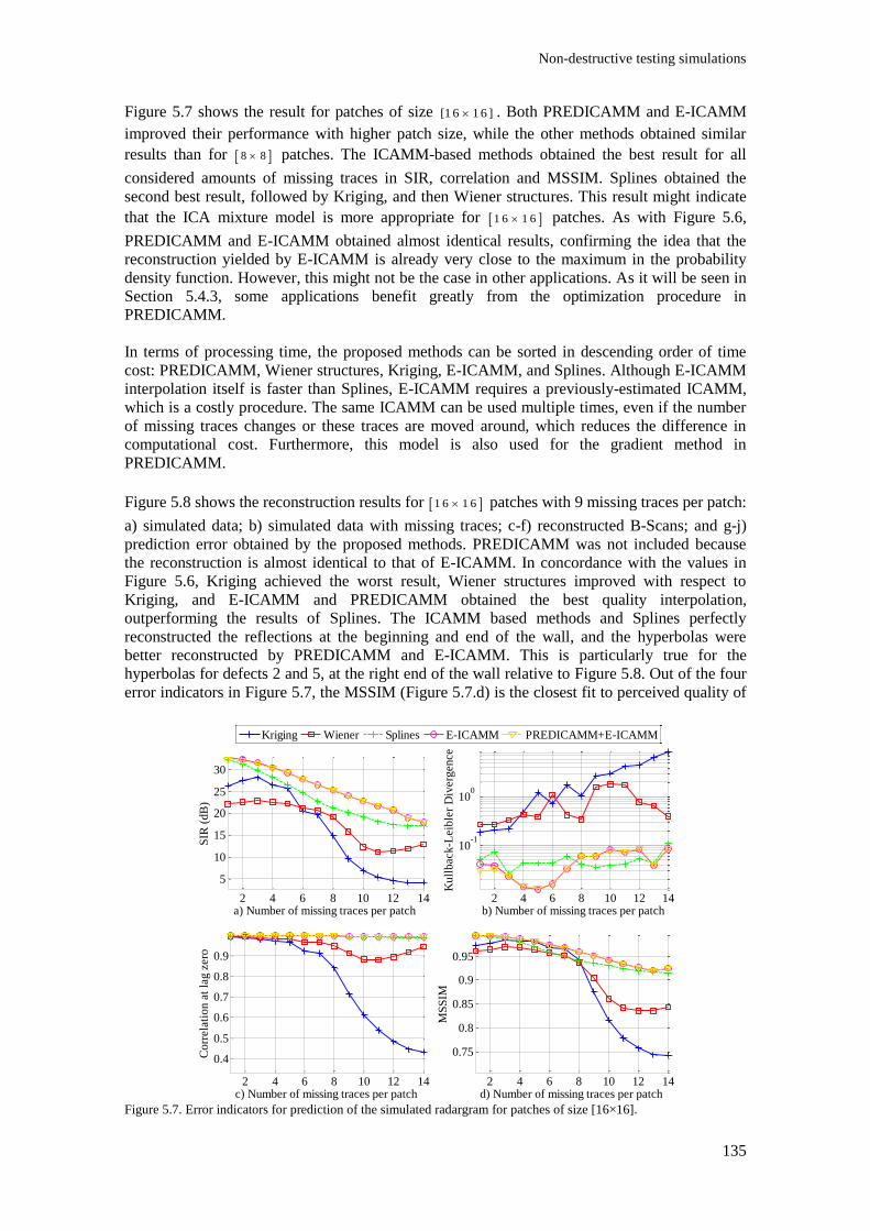
Non-destructive testing simulations
135
Figure 5.7 shows the result for patches of size [1 6 1 6 ] . Both PREDICAMM and E-ICAMM
improved their performance with higher patch size, while the other methods obtained similar
results than for 8 8 patches. The ICAMM-based methods obtained the best result for all
considered amounts of missing traces in SIR, correlation and MSSIM. Splines obtained the
second best result, followed by Kriging, and then Wiener structures. This result might indicate
that the ICA mixture model is more appropriate for 1 6 1 6 patches. As with Figure 5.6,
PREDICAMM and E-ICAMM obtained almost identical results, confirming the idea that the
reconstruction yielded by E-ICAMM is already very close to the maximum in the probability
density function. However, this might not be the case in other applications. As it will be seen in
Section 5.4.3, some applications benefit greatly from the optimization procedure in
PREDICAMM.
In terms of processing time, the proposed methods can be sorted in descending order of time
cost: PREDICAMM, Wiener structures, Kriging, E-ICAMM, and Splines. Although E-ICAMM
interpolation itself is faster than Splines, E-ICAMM requires a previously-estimated ICAMM,
which is a costly procedure. The same ICAMM can be used multiple times, even if the number
of missing traces changes or these traces are moved around, which reduces the difference in
computational cost. Furthermore, this model is also used for the gradient method in
PREDICAMM.
Figure 5.8 shows the reconstruction results for 1 6 1 6 patches with 9 missing traces per patch:
a) simulated data; b) simulated data with missing traces; c-f) reconstructed B-Scans; and g-j)
prediction error obtained by the proposed methods. PREDICAMM was not included because
the reconstruction is almost identical to that of E-ICAMM. In concordance with the values in
Figure 5.6, Kriging achieved the worst result, Wiener structures improved with respect to
Kriging, and E-ICAMM and PREDICAMM obtained the best quality interpolation,
outperforming the results of Splines. The ICAMM based methods and Splines perfectly
reconstructed the reflections at the beginning and end of the wall, and the hyperbolas were
better reconstructed by PREDICAMM and E-ICAMM. This is particularly true for the
hyperbolas for defects 2 and 5, at the right end of the wall relative to Figure 5.8. Out of the four
error indicators in Figure 5.7, the MSSIM (Figure 5.7.d) is the closest fit to perceived quality of
Figure 5.7. Error indicators for prediction of the simulated radargram for patches of size [16×16].
2 4 6 8 10 12 14
5
10
15
20
25
30
a) Number of missing traces per patch
SIR
(d
B)
2 4 6 8 10 12 14
10-1
100
b) Number of missing traces per patch
Ku
llb
ack
-Leib
ler
Div
erg
en
ce
2 4 6 8 10 12 14
0.4
0.5
0.6
0.7
0.8
0.9
c) Number of missing traces per patch
Co
rrela
tio
n a
t la
g z
ero
2 4 6 8 10 12 14
0.75
0.8
0.85
0.9
0.95
d) Number of missing traces per patch
MS
SIM
Kriging Wiener Splines E-ICAMM PREDICAMM+E-ICAMM
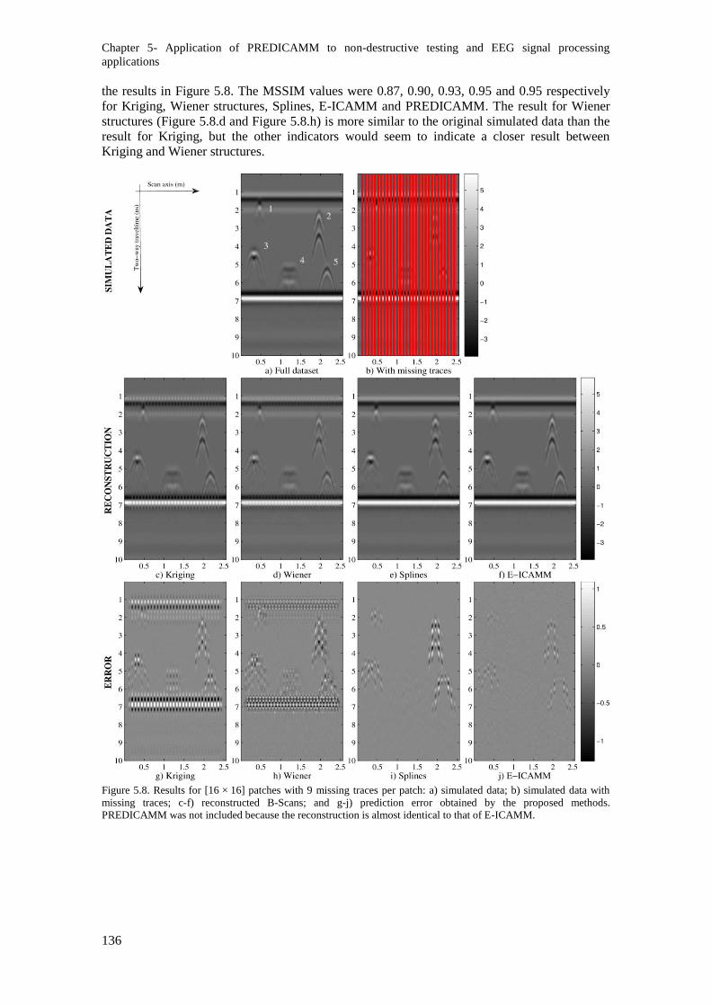
Chapter 5- Application of PREDICAMM to non-destructive testing and EEG signal processing
applications
136
the results in Figure 5.8. The MSSIM values were 0.87, 0.90, 0.93, 0.95 and 0.95 respectively
for Kriging, Wiener structures, Splines, E-ICAMM and PREDICAMM. The result for Wiener
structures (Figure 5.8.d and Figure 5.8.h) is more similar to the original simulated data than the
result for Kriging, but the other indicators would seem to indicate a closer result between
Kriging and Wiener structures.
Figure 5.8. Results for [16 × 16] patches with 9 missing traces per patch: a) simulated data; b) simulated data with
missing traces; c-f) reconstructed B-Scans; and g-j) prediction error obtained by the proposed methods.
PREDICAMM was not included because the reconstruction is almost identical to that of E-ICAMM.
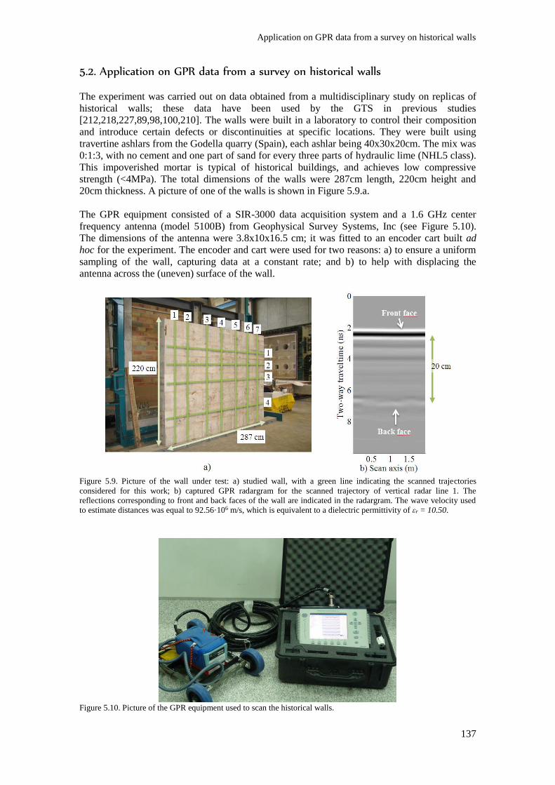
Application on GPR data from a survey on historical walls
137
5.2. Application on GPR data from a survey on historical walls
The experiment was carried out on data obtained from a multidisciplinary study on replicas of
historical walls; these data have been used by the GTS in previous studies
[212,218,227,89,98,100,210]. The walls were built in a laboratory to control their composition
and introduce certain defects or discontinuities at specific locations. They were built using
travertine ashlars from the Godella quarry (Spain), each ashlar being 40x30x20cm. The mix was
0:1:3, with no cement and one part of sand for every three parts of hydraulic lime (NHL5 class).
This impoverished mortar is typical of historical buildings, and achieves low compressive
strength (<4MPa). The total dimensions of the walls were 287cm length, 220cm height and
20cm thickness. A picture of one of the walls is shown in Figure 5.9.a.
The GPR equipment consisted of a SIR-3000 data acquisition system and a 1.6 GHz center
frequency antenna (model 5100B) from Geophysical Survey Systems, Inc (see Figure 5.10).
The dimensions of the antenna were 3.8x10x16.5 cm; it was fitted to an encoder cart built ad
hoc for the experiment. The encoder and cart were used for two reasons: a) to ensure a uniform
sampling of the wall, capturing data at a constant rate; and b) to help with displacing the
antenna across the (uneven) surface of the wall.
Figure 5.9. Picture of the wall under test: a) studied wall, with a green line indicating the scanned trajectories
considered for this work; b) captured GPR radargram for the scanned trajectory of vertical radar line 1. The
reflections corresponding to front and back faces of the wall are indicated in the radargram. The wave velocity used
to estimate distances was equal to 92.56·106 m/s, which is equivalent to a dielectric permittivity of εr = 10.50.
Figure 5.10. Picture of the GPR equipment used to scan the historical walls.
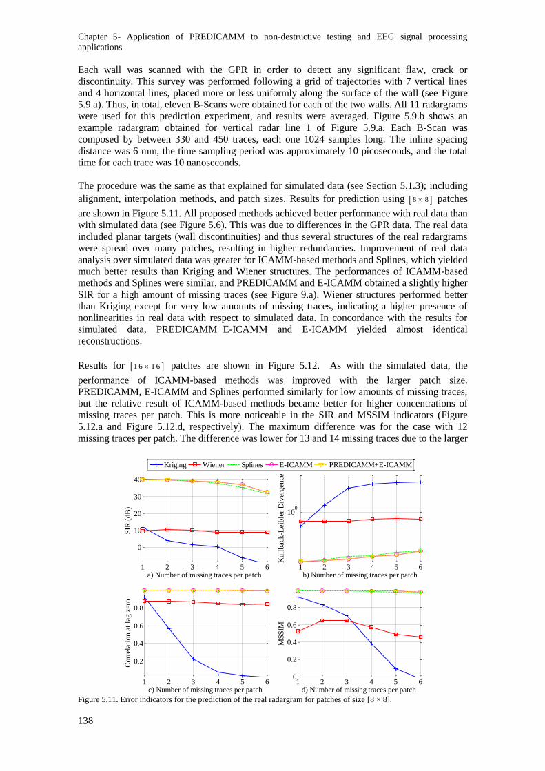
Chapter 5- Application of PREDICAMM to non-destructive testing and EEG signal processing
applications
138
Each wall was scanned with the GPR in order to detect any significant flaw, crack or
discontinuity. This survey was performed following a grid of trajectories with 7 vertical lines
and 4 horizontal lines, placed more or less uniformly along the surface of the wall (see Figure
5.9.a). Thus, in total, eleven B-Scans were obtained for each of the two walls. All 11 radargrams
were used for this prediction experiment, and results were averaged. Figure 5.9.b shows an
example radargram obtained for vertical radar line 1 of Figure 5.9.a. Each B-Scan was
composed by between 330 and 450 traces, each one 1024 samples long. The inline spacing
distance was 6 mm, the time sampling period was approximately 10 picoseconds, and the total
time for each trace was 10 nanoseconds.
The procedure was the same as that explained for simulated data (see Section 5.1.3); including
alignment, interpolation methods, and patch sizes. Results for prediction using 8 8 patches
are shown in Figure 5.11. All proposed methods achieved better performance with real data than
with simulated data (see Figure 5.6). This was due to differences in the GPR data. The real data
included planar targets (wall discontinuities) and thus several structures of the real radargrams
were spread over many patches, resulting in higher redundancies. Improvement of real data
analysis over simulated data was greater for ICAMM-based methods and Splines, which yielded
much better results than Kriging and Wiener structures. The performances of ICAMM-based
methods and Splines were similar, and PREDICAMM and E-ICAMM obtained a slightly higher
SIR for a high amount of missing traces (see Figure 9.a). Wiener structures performed better
than Kriging except for very low amounts of missing traces, indicating a higher presence of
nonlinearities in real data with respect to simulated data. In concordance with the results for
simulated data, PREDICAMM+E-ICAMM and E-ICAMM yielded almost identical
reconstructions.
Results for 1 6 1 6 patches are shown in Figure 5.12. As with the simulated data, the
performance of ICAMM-based methods was improved with the larger patch size.
PREDICAMM, E-ICAMM and Splines performed similarly for low amounts of missing traces,
but the relative result of ICAMM-based methods became better for higher concentrations of
missing traces per patch. This is more noticeable in the SIR and MSSIM indicators (Figure
5.12.a and Figure 5.12.d, respectively). The maximum difference was for the case with 12
missing traces per patch. The difference was lower for 13 and 14 missing traces due to the larger
Figure 5.11. Error indicators for the prediction of the real radargram for patches of size [8 × 8].
1 2 3 4 5 6
0
10
20
30
40
a) Number of missing traces per patch
SIR
(d
B)
1 2 3 4 5 6
100
b) Number of missing traces per patch
Ku
llb
ack
-Leib
ler
Div
erg
en
ce
1 2 3 4 5 6
0.2
0.4
0.6
0.8
c) Number of missing traces per patch
Co
rrela
tio
n a
t la
g z
ero
1 2 3 4 5 60
0.2
0.4
0.6
0.8
d) Number of missing traces per patch
MS
SIM
Kriging Wiener Splines E-ICAMM PREDICAMM+E-ICAMM
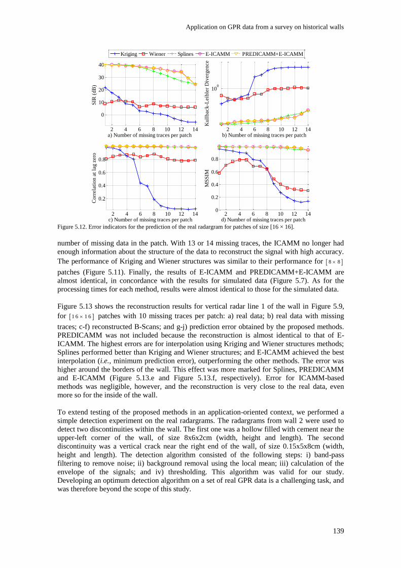
Application on GPR data from a survey on historical walls
139
Figure 5.12. Error indicators for the prediction of the real radargram for patches of size [16 × 16].
number of missing data in the patch. With 13 or 14 missing traces, the ICAMM no longer had
enough information about the structure of the data to reconstruct the signal with high accuracy.
The performance of Kriging and Wiener structures was similar to their performance for 8 8
patches (Figure 5.11). Finally, the results of E-ICAMM and PREDICAMM+E-ICAMM are
almost identical, in concordance with the results for simulated data (Figure 5.7). As for the
processing times for each method, results were almost identical to those for the simulated data.
Figure 5.13 shows the reconstruction results for vertical radar line 1 of the wall in Figure 5.9,
for 1 6 1 6 patches with 10 missing traces per patch: a) real data; b) real data with missing
traces; c-f) reconstructed B-Scans; and g-j) prediction error obtained by the proposed methods.
PREDICAMM was not included because the reconstruction is almost identical to that of E-
ICAMM. The highest errors are for interpolation using Kriging and Wiener structures methods;
Splines performed better than Kriging and Wiener structures; and E-ICAMM achieved the best
interpolation (i.e., minimum prediction error), outperforming the other methods. The error was
higher around the borders of the wall. This effect was more marked for Splines, PREDICAMM
and E-ICAMM (Figure 5.13.e and Figure 5.13.f, respectively). Error for ICAMM-based
methods was negligible, however, and the reconstruction is very close to the real data, even
more so for the inside of the wall.
To extend testing of the proposed methods in an application-oriented context, we performed a
simple detection experiment on the real radargrams. The radargrams from wall 2 were used to
detect two discontinuities within the wall. The first one was a hollow filled with cement near the
upper-left corner of the wall, of size 8x6x2cm (width, height and length). The second
discontinuity was a vertical crack near the right end of the wall, of size 0.15x5x8cm (width,
height and length). The detection algorithm consisted of the following steps: i) band-pass
filtering to remove noise; ii) background removal using the local mean; iii) calculation of the
envelope of the signals; and iv) thresholding. This algorithm was valid for our study.
Developing an optimum detection algorithm on a set of real GPR data is a challenging task, and
was therefore beyond the scope of this study.
2 4 6 8 10 12 14
0
10
20
30
40
a) Number of missing traces per patch
SIR
(d
B)
2 4 6 8 10 12 14
100
b) Number of missing traces per patch
Ku
llb
ack
-Leib
ler
Div
erg
en
ce
2 4 6 8 10 12 14
0.2
0.4
0.6
0.8
c) Number of missing traces per patch
Co
rrela
tio
n a
t la
g z
ero
2 4 6 8 10 12 140
0.2
0.4
0.6
0.8
d) Number of missing traces per patch
MS
SIM
Kriging Wiener Splines E-ICAMM PREDICAMM+E-ICAMM

Chapter 5- Application of PREDICAMM to non-destructive testing and EEG signal processing
applications
140
The detection algorithm was used on the full data set, and with the reconstructed results for the
case with 1 6 1 6 patches and 12 missing traces per patch. The detection results, summarized
by the area under the ROC (Receiver Operating Characteristic) curve, were as follows: 0.6588
(real data), 0.6586 (reconstruction with PREDICAMM+E-ICAMM), 0.6586 (reconstruction
with E-ICAMM), 0.6323 (reconstruction with Splines), 0.5546 (reconstruction with Kriging),
and 0.5259 (reconstruction with Wiener structures). E-ICAMM yielded results that were
consistently almost identical to those of the data without missing traces. Splines yielded the next
best result, and Kriging and Wiener structures yielded the worst detection rates. These results
are in concordance with results in Figure 5.13, showing that a good interpolation can help with
subsequent GPR processing steps.
Figure 5.13. Results for vertical radar line 1 of the wall in Figure 5.9, for [16 × 16] patches with 10 missing traces per
patch: a) real data; b) real data with missing traces; c-f) reconstructed B-Scans; and g-j) prediction error obtained by
the proposed methods. Amplitude was normalized to unit power. PREDICAMM was not included because the
reconstruction is almost identical to that of E-ICAMM.
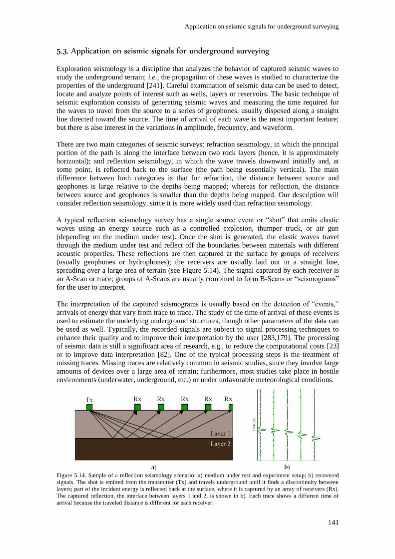
Application on seismic signals for underground surveying
141
5.3. Application on seismic signals for underground surveying
Exploration seismology is a discipline that analyzes the behavior of captured seismic waves to
study the underground terrain; i.e., the propagation of these waves is studied to characterize the
properties of the underground [241]. Careful examination of seismic data can be used to detect,
locate and analyze points of interest such as wells, layers or reservoirs. The basic technique of
seismic exploration consists of generating seismic waves and measuring the time required for
the waves to travel from the source to a series of geophones, usually disposed along a straight
line directed toward the source. The time of arrival of each wave is the most important feature;
but there is also interest in the variations in amplitude, frequency, and waveform.
There are two main categories of seismic surveys: refraction seismology, in which the principal
portion of the path is along the interface between two rock layers (hence, it is approximately
horizontal); and reflection seismology, in which the wave travels downward initially and, at
some point, is reflected back to the surface (the path being essentially vertical). The main
difference between both categories is that for refraction, the distance between source and
geophones is large relative to the depths being mapped; whereas for reflection, the distance
between source and geophones is smaller than the depths being mapped. Our description will
consider reflection seismology, since it is more widely used than refraction seismology.
A typical reflection seismology survey has a single source event or “shot” that emits elastic
waves using an energy source such as a controlled explosion, thumper truck, or air gun
(depending on the medium under test). Once the shot is generated, the elastic waves travel
through the medium under test and reflect off the boundaries between materials with different
acoustic properties. These reflections are then captured at the surface by groups of receivers
(usually geophones or hydrophones); the receivers are usually laid out in a straight line,
spreading over a large area of terrain (see Figure 5.14). The signal captured by each receiver is
an A-Scan or trace; groups of A-Scans are usually combined to form B-Scans or “seismograms”
for the user to interpret.
The interpretation of the captured seismograms is usually based on the detection of “events,”
arrivals of energy that vary from trace to trace. The study of the time of arrival of these events is
used to estimate the underlying underground structures, though other parameters of the data can
be used as well. Typically, the recorded signals are subject to signal processing techniques to
enhance their quality and to improve their interpretation by the user [283,179]. The processing
of seismic data is still a significant area of research, e.g., to reduce the computational costs [23]
or to improve data interpretation [82]. One of the typical processing steps is the treatment of
missing traces. Missing traces are relatively common in seismic studies, since they involve large
amounts of devices over a large area of terrain; furthermore, most studies take place in hostile
environments (underwater, underground, etc.) or under unfavorable meteorological conditions.
Figure 5.14. Sample of a reflection seismology scenario: a) medium under test and experiment setup; b) recovered
signals. The shot is emitted from the transmitter (Tx) and travels underground until it finds a discontinuity between
layers; part of the incident energy is reflected back at the surface, where it is captured by an array of receivers (Rx).
The captured reflection, the interface between layers 1 and 2, is shown in b). Each trace shows a different time of
arrival because the traveled distance is different for each receiver.
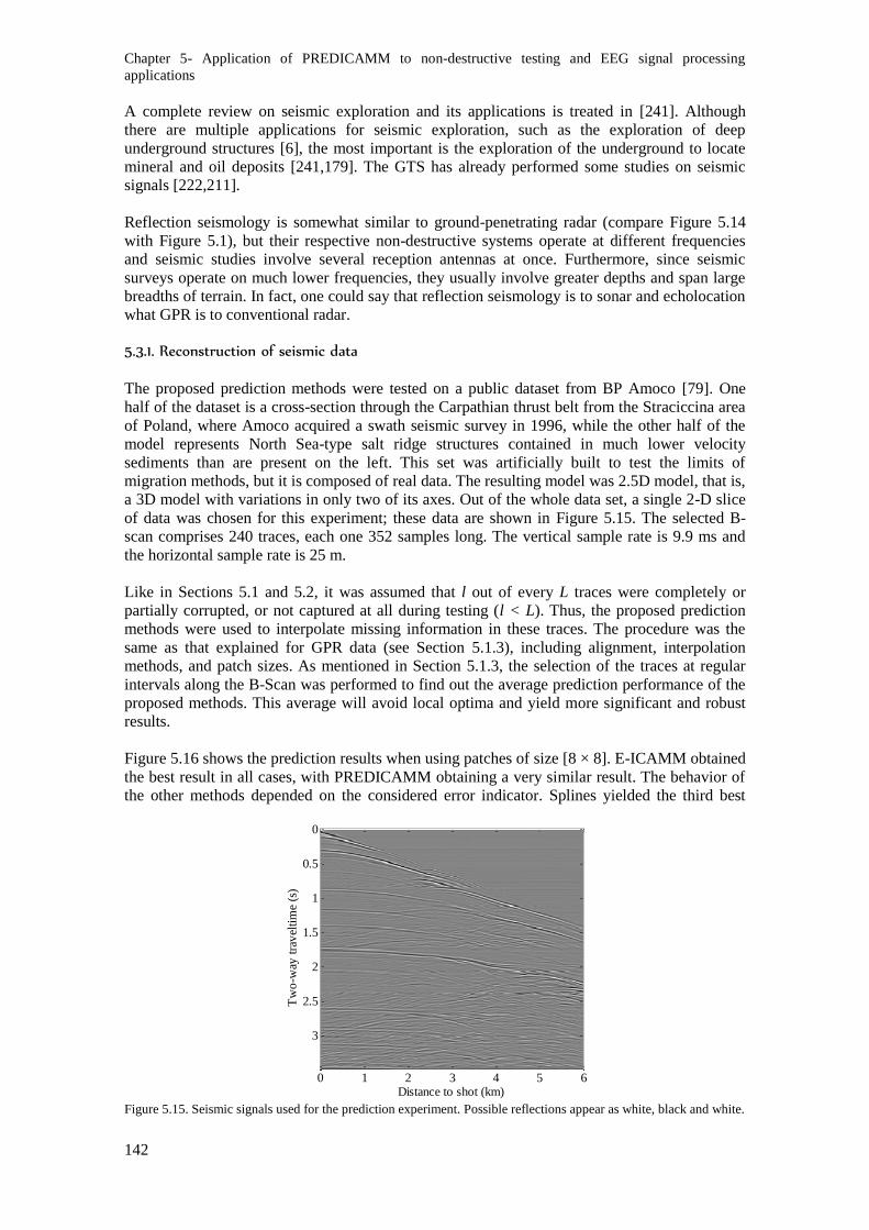
Chapter 5- Application of PREDICAMM to non-destructive testing and EEG signal processing
applications
142
A complete review on seismic exploration and its applications is treated in [241]. Although
there are multiple applications for seismic exploration, such as the exploration of deep
underground structures [6], the most important is the exploration of the underground to locate
mineral and oil deposits [241,179]. The GTS has already performed some studies on seismic
signals [222,211].
Reflection seismology is somewhat similar to ground-penetrating radar (compare Figure 5.14
with Figure 5.1), but their respective non-destructive systems operate at different frequencies
and seismic studies involve several reception antennas at once. Furthermore, since seismic
surveys operate on much lower frequencies, they usually involve greater depths and span large
breadths of terrain. In fact, one could say that reflection seismology is to sonar and echolocation
what GPR is to conventional radar.
5.3.1. Reconstruction of seismic data
The proposed prediction methods were tested on a public dataset from BP Amoco [79]. One
half of the dataset is a cross-section through the Carpathian thrust belt from the Straciccina area
of Poland, where Amoco acquired a swath seismic survey in 1996, while the other half of the
model represents North Sea-type salt ridge structures contained in much lower velocity
sediments than are present on the left. This set was artificially built to test the limits of
migration methods, but it is composed of real data. The resulting model was 2.5D model, that is,
a 3D model with variations in only two of its axes. Out of the whole data set, a single 2-D slice
of data was chosen for this experiment; these data are shown in Figure 5.15. The selected B-
scan comprises 240 traces, each one 352 samples long. The vertical sample rate is 9.9 ms and
the horizontal sample rate is 25 m.
Like in Sections 5.1 and 5.2, it was assumed that l out of every L traces were completely or
partially corrupted, or not captured at all during testing (l < L). Thus, the proposed prediction
methods were used to interpolate missing information in these traces. The procedure was the
same as that explained for GPR data (see Section 5.1.3), including alignment, interpolation
methods, and patch sizes. As mentioned in Section 5.1.3, the selection of the traces at regular
intervals along the B-Scan was performed to find out the average prediction performance of the
proposed methods. This average will avoid local optima and yield more significant and robust
results.
Figure 5.16 shows the prediction results when using patches of size [8 × 8]. E-ICAMM obtained
the best result in all cases, with PREDICAMM obtaining a very similar result. The behavior of
the other methods depended on the considered error indicator. Splines yielded the third best
Figure 5.15. Seismic signals used for the prediction experiment. Possible reflections appear as white, black and white.
Distance to shot (km)
Tw
o-w
ay t
rav
elti
me
(s)
0 1 2 3 4 5 6
0
0.5
1
1.5
2
2.5
3
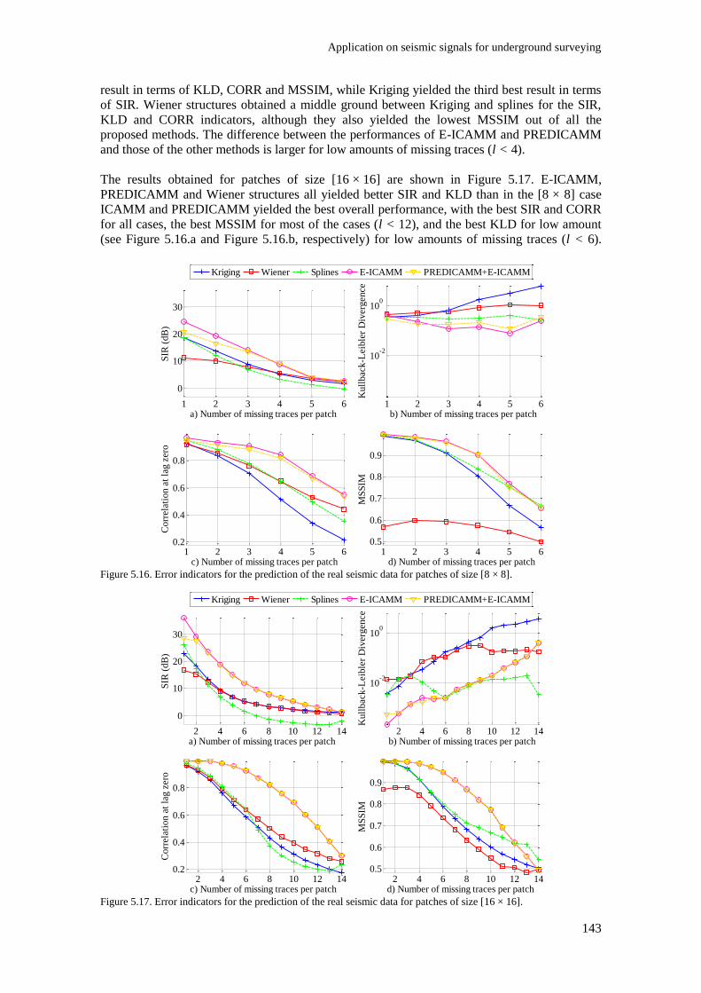
Application on seismic signals for underground surveying
143
result in terms of KLD, CORR and MSSIM, while Kriging yielded the third best result in terms
of SIR. Wiener structures obtained a middle ground between Kriging and splines for the SIR,
KLD and CORR indicators, although they also yielded the lowest MSSIM out of all the
proposed methods. The difference between the performances of E-ICAMM and PREDICAMM
and those of the other methods is larger for low amounts of missing traces (l < 4).
The results obtained for patches of size [16 × 16] are shown in Figure 5.17. E-ICAMM,
PREDICAMM and Wiener structures all yielded better SIR and KLD than in the [8 × 8] case
ICAMM and PREDICAMM yielded the best overall performance, with the best SIR and CORR
for all cases, the best MSSIM for most of the cases (l < 12), and the best KLD for low amount
(see Figure 5.16.a and Figure 5.16.b, respectively) for low amounts of missing traces (l < 6).
Figure 5.16. Error indicators for the prediction of the real seismic data for patches of size [8 × 8].
Figure 5.17. Error indicators for the prediction of the real seismic data for patches of size [16 × 16].
1 2 3 4 5 6
0
10
20
30
a) Number of missing traces per patch
SIR
(d
B)
1 2 3 4 5 6
10-2
100
b) Number of missing traces per patch
Ku
llb
ack
-Leib
ler
Div
erg
en
ce
1 2 3 4 5 60.2
0.4
0.6
0.8
c) Number of missing traces per patch
Co
rrela
tio
n a
t la
g z
ero
1 2 3 4 5 60.5
0.6
0.7
0.8
0.9
d) Number of missing traces per patch
MS
SIM
Kriging Wiener Splines E-ICAMM PREDICAMM+E-ICAMM
2 4 6 8 10 12 14
0
10
20
30
a) Number of missing traces per patch
SIR
(d
B)
2 4 6 8 10 12 14
10-2
100
b) Number of missing traces per patch
Ku
llb
ack
-Leib
ler
Div
erg
en
ce
2 4 6 8 10 12 140.2
0.4
0.6
0.8
c) Number of missing traces per patch
Co
rrela
tio
n a
t la
g z
ero
2 4 6 8 10 12 140.5
0.6
0.7
0.8
0.9
d) Number of missing traces per patch
MS
SIM
Kriging Wiener Splines E-ICAMM PREDICAMM+E-ICAMM
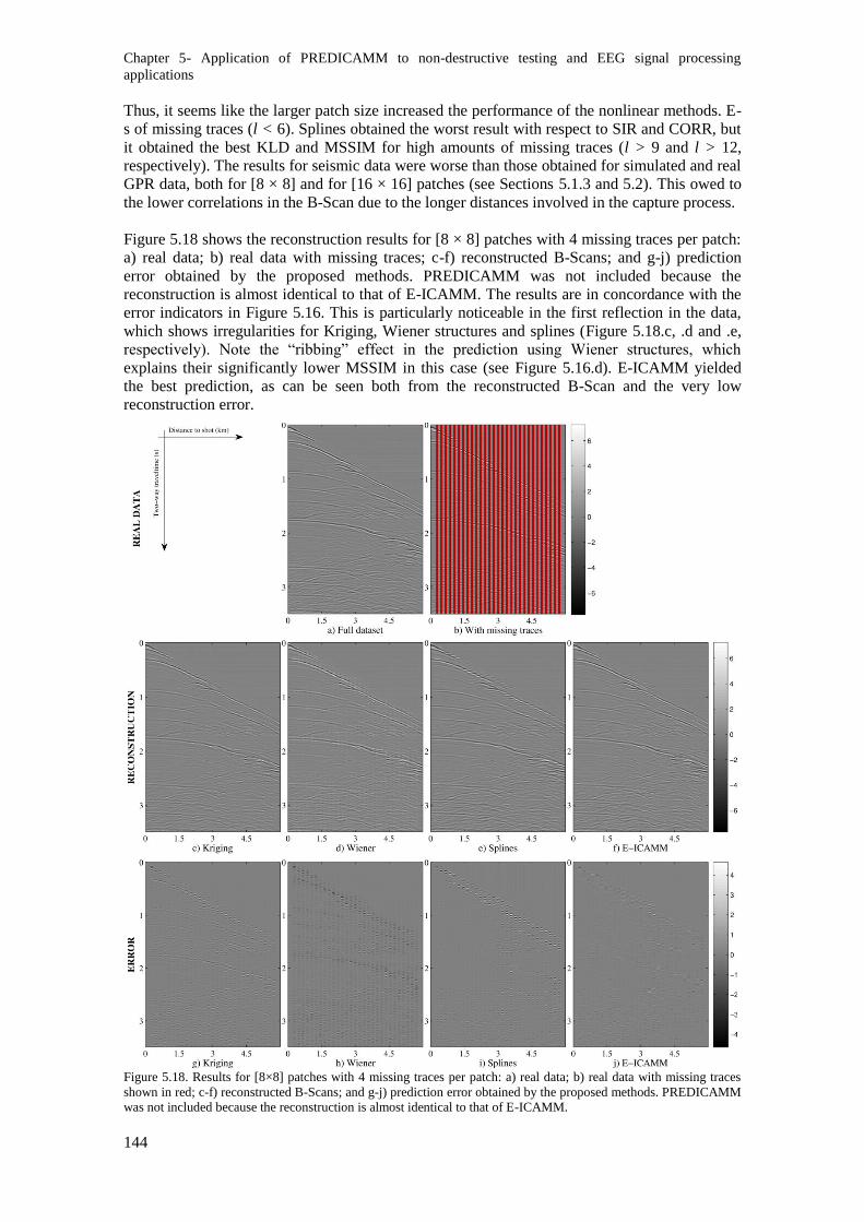
Chapter 5- Application of PREDICAMM to non-destructive testing and EEG signal processing
applications
144
Thus, it seems like the larger patch size increased the performance of the nonlinear methods. E-
s of missing traces (l < 6). Splines obtained the worst result with respect to SIR and CORR, but
it obtained the best KLD and MSSIM for high amounts of missing traces (l > 9 and l > 12,
respectively). The results for seismic data were worse than those obtained for simulated and real
GPR data, both for [8 × 8] and for [16 × 16] patches (see Sections 5.1.3 and 5.2). This owed to
the lower correlations in the B-Scan due to the longer distances involved in the capture process.
Figure 5.18 shows the reconstruction results for [8 × 8] patches with 4 missing traces per patch:
a) real data; b) real data with missing traces; c-f) reconstructed B-Scans; and g-j) prediction
error obtained by the proposed methods. PREDICAMM was not included because the
reconstruction is almost identical to that of E-ICAMM. The results are in concordance with the
error indicators in Figure 5.16. This is particularly noticeable in the first reflection in the data,
which shows irregularities for Kriging, Wiener structures and splines (Figure 5.18.c, .d and .e,
respectively). Note the “ribbing” effect in the prediction using Wiener structures, which
explains their significantly lower MSSIM in this case (see Figure 5.16.d). E-ICAMM yielded
the best prediction, as can be seen both from the reconstructed B-Scan and the very low
reconstruction error.
Figure 5.18. Results for [8×8] patches with 4 missing traces per patch: a) real data; b) real data with missing traces
shown in red; c-f) reconstructed B-Scans; and g-j) prediction error obtained by the proposed methods. PREDICAMM
was not included because the reconstruction is almost identical to that of E-ICAMM.

Application on electroencephalographic signals
145
5.4. Application on electroencephalographic signals
Electroencephalographic signals are recordings of surface brain electrical activity taken at the
scalp, where each sensor captures the combined signal from multiple neurons of the brain [185].
The study of EEG signals is a useful clinical tool because some illnesses, typically seizures and
sleep disorders, produce abnormal electric patterns in the electrical activity of the brain that can
be identified by an expert. Even though there are other techniques for the exploration of the
human brain, such as magnetic resonance (MRI), functional magnetic resonance (fMRI) and
positron emission tomography (PET), EEG remains the subject of much research on brain
activity and a valuable tool for clinical analysis. The main reasons for the use of EEG are the
lower hardware cost of the device, the higher temporal resolution of EEG when compared to
other available techniques, and the maturity of EEG analysis. Research on EEG data started in
the late years of the 19th century, although digital processing techniques were not used until the
late 1990s [258].
Independent component analysis and other blind source separation techniques have been
successfully used for the modeling and processing of EEG and other biological signals. For
instance, ICA has been used to separate fetal and maternal electrocardiograms (ECG)
[286,285,233], detect atrial fibrillation [284,92], and analyze high-density ECG [292].
The first applications of ICA to EEG signals took place during the late 1990s [258]. These
works introduced the assumption that each EEG channel is composed by the mixture of a
number of non-Gaussian sources [159,160]. Furthermore, it is assumed that this mixture is
generated by the mixture of signals from several neurons due to the own conductivity of the
head, and that this mixing is almost instantaneous in nature. In ICA, EEG signals are modeled
as a mixture of independent but spatially fixed sources, with each source being either a point
source or a distributed source spanning over an area of the brain. Later works seem to confirm
that not only is it possible to separate time signals, but it is also possible to locate them on the
surface of the head [190]. This spatial location is far from perfect, but it has been shown to be a
very useful pre-processing step for other source location algorithms (for instance, [291]).
Another important application of ICA makes use of the recovered sources to model the EEG
signal, allowing the extraction of sources of a given kind, e.g., evoked potential signals
[161,162]. This source separation method is statistical in nature and therefore it can correctly
separate signals that overlap across time and/or frequency (a probabilistic filter, as it were). This
application can be used to remove unimportant signals and reduce the workload of the expert
during exploration. Moreover, it can also be used for automatic diagnosis of illnesses such as
ADHD (Attention Deficit Hyperactivity Disorder) or sleep disorders [180,230]. There are also
works on the application of ICA to the separation of fMRI signals [168]. In this thesis, however,
we will only consider EEG signals.
Source separation by ICA can also be used for artifact removal, since there are several artifacts
that can be safely assumed to be independent from EEG data [128]. There are several works on
this topic, ranging from supervised artifact removal [128] to fully automatic artifact detection
and removal [186]. A good review of the applications of ICA to EEG signal processing can be
found in [127].
One of the main research topics on the application of ICA to EEG signals is the dynamic
modeling of brain oscillations in humans [230,189,109,61] and lab rats [232,10]. This research
attempts to combine the advantages of independent component analysis with the capabilities of
certain dynamic models to deal with the temporal variability of the EEG. For instance, some
representative examples are the study of developmental differences in the saccadic contingent
negative variation [138], EEG and event-related potential (ERP) data [162,277], and removal of
artifacts in the EEG signal [44]. The GTS has already published some works in this area [230].
EEG data will also be explored in Chapter 6, where we will apply the methods proposed in
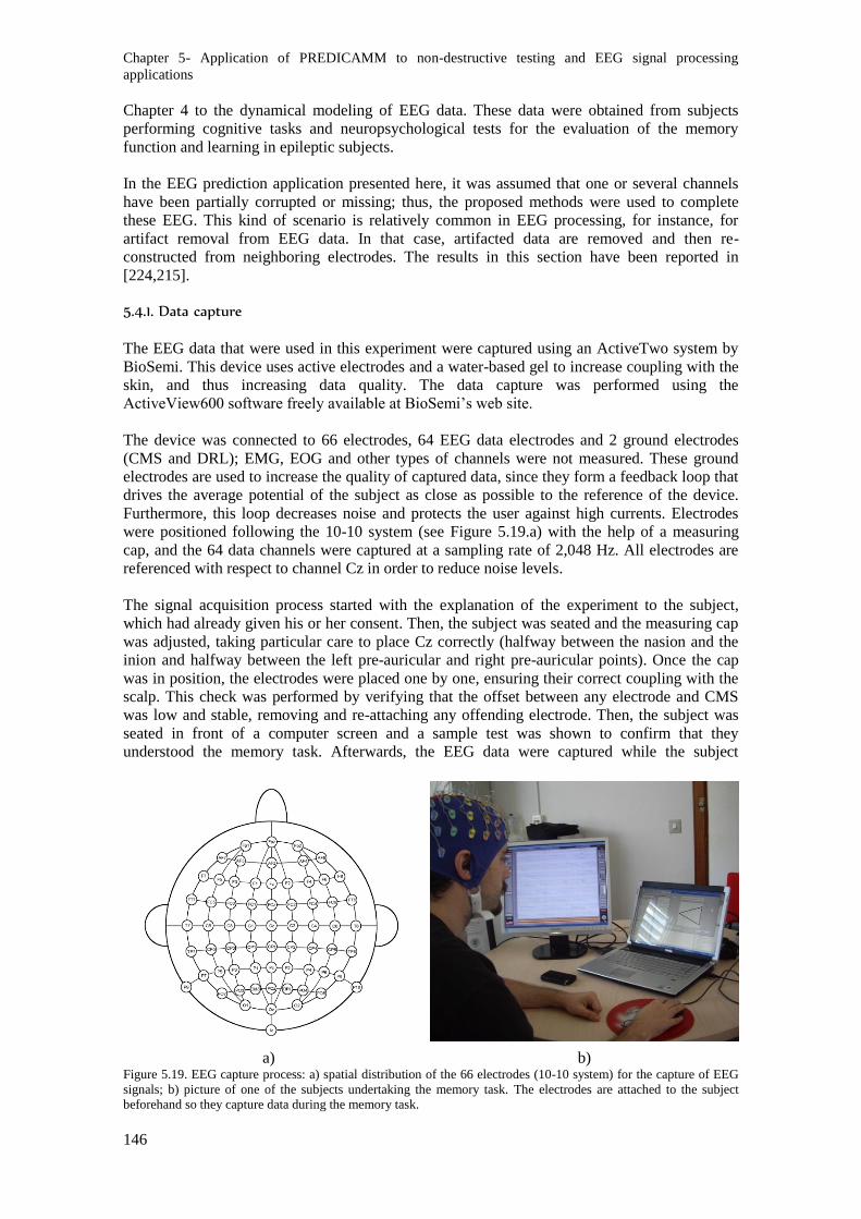
Chapter 5- Application of PREDICAMM to non-destructive testing and EEG signal processing
applications
146
Chapter 4 to the dynamical modeling of EEG data. These data were obtained from subjects
performing cognitive tasks and neuropsychological tests for the evaluation of the memory
function and learning in epileptic subjects.
In the EEG prediction application presented here, it was assumed that one or several channels
have been partially corrupted or missing; thus, the proposed methods were used to complete
these EEG. This kind of scenario is relatively common in EEG processing, for instance, for
artifact removal from EEG data. In that case, artifacted data are removed and then re-
constructed from neighboring electrodes. The results in this section have been reported in
[224,215].
5.4.1. Data capture
The EEG data that were used in this experiment were captured using an ActiveTwo system by
BioSemi. This device uses active electrodes and a water-based gel to increase coupling with the
skin, and thus increasing data quality. The data capture was performed using the
ActiveView600 software freely available at BioSemi’s web site.
The device was connected to 66 electrodes, 64 EEG data electrodes and 2 ground electrodes
(CMS and DRL); EMG, EOG and other types of channels were not measured. These ground
electrodes are used to increase the quality of captured data, since they form a feedback loop that
drives the average potential of the subject as close as possible to the reference of the device.
Furthermore, this loop decreases noise and protects the user against high currents. Electrodes
were positioned following the 10-10 system (see Figure 5.19.a) with the help of a measuring
cap, and the 64 data channels were captured at a sampling rate of 2,048 Hz. All electrodes are
referenced with respect to channel Cz in order to reduce noise levels.
The signal acquisition process started with the explanation of the experiment to the subject,
which had already given his or her consent. Then, the subject was seated and the measuring cap
was adjusted, taking particular care to place Cz correctly (halfway between the nasion and the
inion and halfway between the left pre-auricular and right pre-auricular points). Once the cap
was in position, the electrodes were placed one by one, ensuring their correct coupling with the
scalp. This check was performed by verifying that the offset between any electrode and CMS
was low and stable, removing and re-attaching any offending electrode. Then, the subject was
seated in front of a computer screen and a sample test was shown to confirm that they
understood the memory task. Afterwards, the EEG data were captured while the subject
a) b) Figure 5.19. EEG capture process: a) spatial distribution of the 66 electrodes (10-10 system) for the capture of EEG
signals; b) picture of one of the subjects undertaking the memory task. The electrodes are attached to the subject
beforehand so they capture data during the memory task.
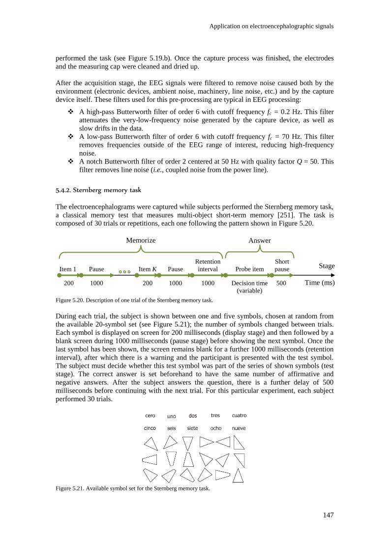
Application on electroencephalographic signals
147
performed the task (see Figure 5.19.b). Once the capture process was finished, the electrodes
and the measuring cap were cleaned and dried up.
After the acquisition stage, the EEG signals were filtered to remove noise caused both by the
environment (electronic devices, ambient noise, machinery, line noise, etc.) and by the capture
device itself. These filters used for this pre-processing are typical in EEG processing:
A high-pass Butterworth filter of order 6 with cutoff frequency fc = 0.2 Hz. This filter
attenuates the very-low-frequency noise generated by the capture device, as well as
slow drifts in the data.
A low-pass Butterworth filter of order 6 with cutoff frequency fc = 70 Hz. This filter
removes frequencies outside of the EEG range of interest, reducing high-frequency
noise.
A notch Butterworth filter of order 2 centered at 50 Hz with quality factor Q = 50. This
filter removes line noise (i.e., coupled noise from the power line).
5.4.2. Sternberg memory task
The electroencephalograms were captured while subjects performed the Sternberg memory task,
a classical memory test that measures multi-object short-term memory [251]. The task is
composed of 30 trials or repetitions, each one following the pattern shown in Figure 5.20.
Figure 5.20. Description of one trial of the Sternberg memory task.
During each trial, the subject is shown between one and five symbols, chosen at random from
the available 20-symbol set (see Figure 5.21); the number of symbols changed between trials.
Each symbol is displayed on screen for 200 milliseconds (display stage) and then followed by a
blank screen during 1000 milliseconds (pause stage) before showing the next symbol. Once the
last symbol has been shown, the screen remains blank for a further 1000 milliseconds (retention
interval), after which there is a warning and the participant is presented with the test symbol.
The subject must decide whether this test symbol was part of the series of shown symbols (test
stage). The correct answer is set beforehand to have the same number of affirmative and
negative answers. After the subject answers the question, there is a further delay of 500
milliseconds before continuing with the next trial. For this particular experiment, each subject
performed 30 trials.
Figure 5.21. Available symbol set for the Sternberg memory task.
Retention Short
Item 1 Pause Item K Pause interval Probe item pause
200 1000 200 1000 1000 Decision time 500 (variable)
Stage
Time (ms)
Memorize Answer
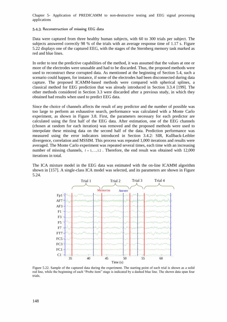
Chapter 5- Application of PREDICAMM to non-destructive testing and EEG signal processing
applications
148
5.4.3. Reconstruction of missing EEG data
Data were captured from three healthy human subjects, with 60 to 300 trials per subject. The
subjects answered correctly 98 % of the trials with an average response time of 1.17 s. Figure
5.22 displays one of the captured EEG, with the stages of the Sternberg memory task marked as
red and blue lines.
In order to test the predictive capabilities of the method, it was assumed that the values at one or
more of the electrodes were unusable and had to be discarded. Thus, the proposed methods were
used to reconstruct these corrupted data. As mentioned at the beginning of Section 5.4, such a
scenario could happen, for instance, if some of the electrodes had been disconnected during data
capture. The proposed ICAMM-based methods were compared with spherical splines, a
classical method for EEG prediction that was already introduced in Section 3.3.4 [199]. The
other methods considered in Section 3.3 were discarded after a previous study, in which they
obtained bad results when used to predict EEG data.
Since the choice of channels affects the result of any predictor and the number of possible was
too large to perform an exhaustive search, performance was calculated with a Monte Carlo
experiment, as shown in Figure 3.8. First, the parameters necessary for each predictor are
calculated using the first half of the EEG data. After estimation, one of the EEG channels
(chosen at random for each iteration) was removed and the proposed methods were used to
interpolate these missing data on the second half of the data. Prediction performance was
measured using the error indicators introduced in Section 3.4.2: SIR, Kullback-Leibler
divergence, correlation and MSSIM. This process was repeated 1,000 iterations and results were
averaged. The Monte Carlo experiment was repeated several times, each time with an increasing
number of missing channels, 1, ...,12l . Therefore, the end result was obtained with 12,000
iterations in total.
The ICA mixture model in the EEG data was estimated with the on-line ICAMM algorithm
shown in [157]. A single-class ICA model was selected, and its parameters are shown in Figure
5.24.
Figure 5.22. Sample of the captured data during the experiment. The starting point of each trial is shown as a solid
red line, while the beginning of each “Probe item” stage is indicated by a dashed blue line. The shown data span four
trials.
35 40 45 50 55 60C1
FC1
FC3
FC5
FT7
F7
F5
F3
F1
AF3
AF7
Fp1
Time (s)
Memorize Answer
Trial 1 Trial 2 Trial 3 Trial 4
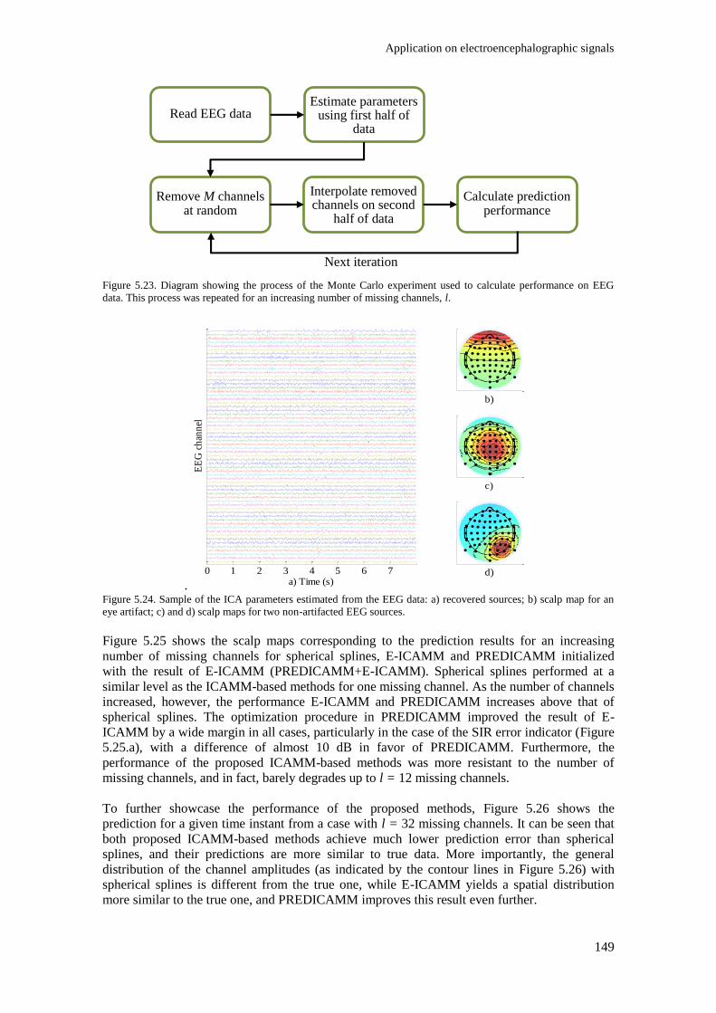
Application on electroencephalographic signals
149
Figure 5.23. Diagram showing the process of the Monte Carlo experiment used to calculate performance on EEG
data. This process was repeated for an increasing number of missing channels, l.
. Figure 5.24. Sample of the ICA parameters estimated from the EEG data: a) recovered sources; b) scalp map for an
eye artifact; c) and d) scalp maps for two non-artifacted EEG sources.
Figure 5.25 shows the scalp maps corresponding to the prediction results for an increasing
number of missing channels for spherical splines, E-ICAMM and PREDICAMM initialized
with the result of E-ICAMM (PREDICAMM+E-ICAMM). Spherical splines performed at a
similar level as the ICAMM-based methods for one missing channel. As the number of channels
increased, however, the performance E-ICAMM and PREDICAMM increases above that of
spherical splines. The optimization procedure in PREDICAMM improved the result of E-
ICAMM by a wide margin in all cases, particularly in the case of the SIR error indicator (Figure
5.25.a), with a difference of almost 10 dB in favor of PREDICAMM. Furthermore, the
performance of the proposed ICAMM-based methods was more resistant to the number of
missing channels, and in fact, barely degrades up to l = 12 missing channels.
To further showcase the performance of the proposed methods, Figure 5.26 shows the
prediction for a given time instant from a case with l = 32 missing channels. It can be seen that
both proposed ICAMM-based methods achieve much lower prediction error than spherical
splines, and their predictions are more similar to true data. More importantly, the general
distribution of the channel amplitudes (as indicated by the contour lines in Figure 5.26) with
spherical splines is different from the true one, while E-ICAMM yields a spatial distribution
more similar to the true one, and PREDICAMM improves this result even further.
0 1 2 3 4 5 6 7a) Time (s)
EE
G c
han
nel
b)
c)
d)
Read EEG data Estimate parameters
using first half of data
Remove M channels at random
Interpolate removed channels on second
half of data
Calculate prediction performance
Next iteration
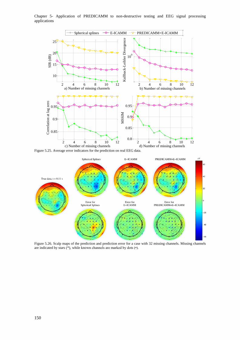
Chapter 5- Application of PREDICAMM to non-destructive testing and EEG signal processing
applications
150
Figure 5.25. Average error indicators for the prediction on real EEG data.
Figure 5.26. Scalp maps of the prediction and prediction error for a case with 32 missing channels. Missing channels
are indicated by stars (*), while known channels are marked by dots (•).
2 4 6 8 10 12
10
15
20
25
a) Number of missing channels
SIR
(dB
)
2 4 6 8 10 12
100
b) Number of missing channels
Ku
llback-L
eib
ler
Div
erg
ence
2 4 6 8 10 12
0.85
0.9
0.95
c) Number of missing channels
Corr
ela
tion a
t la
g z
ero
2 4 6 8 10 120.8
0.85
0.9
0.95
d) Number of missing channels
MS
SIM
Spherical splines E-ICAMM PREDICAMM+E-ICAMM
Conclusions
151
5.5. Conclusions
This chapter presents the application on real data of the prediction methods introduced in
Chapter 3, PREDICAMM and E-ICAMM. Both methods make the assumption that the data can
be modeled using a mixture of independent component analyzers (ICA). Each of these methods
is the optimal predictor with respect to one particular characteristic: PREDICAMM is optimal
with respect to the log-likelihood of the data, while E-ICAMM is optimal with respect to the
mean square error. Both predictors are general-purpose and they can be used in many signal
processing fields. Because of this flexibility, they were tested for the reconstruction of missing
data from three quite different signal processing fields: non-destructive testing, seismic
exploration, and electroencephalography.
First, the proposed methods were tested on a set of simulated NDT data, a synthetic radargram.
In this case, the methods were used to reconstruct several missing traces from the radargram.
This application required the transformation of the two-dimensional signal (B-Scan) to a one-
dimensional signal by a decomposition of the original image into square patches, a process that
we have named alignment. After alignment, E-ICAMM and PREDICAMM were compared
with the state-of-the-art method (Splines), a classical predictor (Kriging), and a nonlinear
predictor (Wiener structures). Two patch sizes were considered, [8 × 8] and [16 × 16], and the
behavior of the proposed methods changed slightly with patch size. For [8 × 8] patches, the
reconstruction yielded by PREDICAMM and E-ICAMM was similar to that obtained by the
state-of-the-art method (Splines), and was better than that of the competing methods for high
amounts of missing traces. The performance of the ICAMM-based methods increased for
[16 × 16] patches, in which case both E-ICAMM and PREDICAMM over-performed Splines
across all estimators (e.g., the SIR obtained by both methods was 3dB higher, on average, than
the SIR obtained by Splines). The proposed methods and Splines always performed better than
the classical predictor, Kriging, and a nonlinear predictor, Wiener structures. This improved
reconstruction was shown by a better reconstruction of the shape of the recovered hyperbolas in
the simulated radargram. For this application, the gradient used in PREDICAMM did not obtain
any significant difference with respect to the initial value provided by E-ICAMM.
The first application of the proposed methods on real data consisted of the reconstruction of real
GPR data from a study on replicas of historical walls. As with the simulated data, the data had
to be aligned prior to prediction, and the result proved to depend on patch size. In this case,
however, performance was different because of the larger presence of planar targets in the real
data. PREDICAMM, E-ICAMM and Splines performed better on the considered set of real data
(9 dB average increase in SIR), while Kriging and Wiener structures performed worse on real
data (8 dB average reduction in SIR). Thus, the difference in performance between both groups
of methods was larger for real data, and the difference between Splines and the proposed
ICAMM-based methods was smaller. Other than these differences, the relative behavior of the
methods was in concordance with the results on simulated data. E-ICAMM and PREDICAMM
performed at a similar level to Splines for [8 × 8] patches, and performed better than Splines for
[16 × 16] patches.
The second application was the reconstruction of missing data from a seismic B-Scan or
seismogram, which was obtained from a public dataset from BP Amoco. Again, the
performance of E-ICAMM and PREDICAMM was compared with that of Splines, Kriging and
Wiener structures. The basic structure of the seismogram is similar to that of the radargram, and
therefore, alignment was required to predict missing data with the proposed methods. The real
seismogram, however, was more complex than the radargram and all the proposed methods
achieved lower performances than they did for the first application. E-ICAMM and
PREDICAMM always performed better than the other considered methods, and Splines usually
performed better than Kriging and Wiener structures. The difference between the proposed
methods and Splines was higher for [16 × 16] patches (8 dB average increase in SIR) than it was
for [16 × 16] patches (4 dB average increase in SIR). Finally, PREDICAMM performed at a

Chapter 5- Application of PREDICAMM to non-destructive testing and EEG signal processing
applications
152
very similar level to E-ICAMM. Other than the general decrease in performance, which was
more marked in the case of Splines, these results are consistent with those obtained on GPR
data.
Finally, E-ICAMM and PREDICAMM were tested for the reconstruction of missing
information from EEG data. These EEG were obtained from healthy human subjects performing
the Sternberg memory task. The proposed methods were used to reconstruct missing data from
one or more EEG channels, a scenario simulating the disconnection of the corresponding
electrodes. In this application, the performance of the proposed methods was compared with
that of the classical interpolator for EEG data, Spherical Splines, which was introduced in
Section 3.3.4. Results showed that PREDICAMM performed better than E-ICAMM, which in
turn performed better than Spherical Splines. These differences were small for one missing
channel, but increased rapidly with the number of missing channels. This behavior owed to the
faster decrease of performance of Spherical Splines, whereas both E-ICAMM and
PREDICAMM were shown to be resistant to the number of missing channels. This point was
shown with an extreme case where half the channels were missing. Even in this case, the
reconstruction yielded by E-ICAMM and PREDICAMM was similar to the true data.
In the results presented in this chapter, PREDICAMM was always initialized with E-ICAMM.
When used on GPR or seismic data, however, PREDICAMM obtained a result that was very
similar to that of E-ICAMM. In these cases, the initial value was already very close to a
(possibly local) maximum in the log-likelihood and PREDICAMM did not iterate, or iterated
only shortly. Conversely, the performance of PREDICAMM did improve greatly over that of
the initial value, E-ICAMM, for the reconstruction of EEG data. ICA techniques have been used
on EEG data for a wide variety of applications, and the estimation of the ICA parameters in this
case is well known. Therefore, it would seem that PREDICAMM performed better in the case
where the ICA mixture model was best fit (EEG data), and not as well when the model was
more complex or less applicable (radargram, seismogram). In the former, the probability
densities estimated from the model were more precise and the maximization procedure in
PREDICAMM was optimal. In the latter, the densities were not as precise and the initial value
was usually close to a local maximum, reducing the usefulness of the gradient optimization step.
Furthermore, the ICA mixture model allows us to model local dependences without
compromising the modeling of global structure. This behavior increases the performance of the
proposed predictors and, at the same time, describes the structure in the data, since the ICAMM
parameters can be studied to gain further knowledge on the data. This will be expanded upon in
Chapter 6, where we will present the application of dynamic modeling methods to cognitive
tasks and neuropsychological tests for the evaluation of the memory function and learning in
epileptic subjects.

153
Application of G- and UG-SICAMM to EEG signal processing 6


155
- Application of G- and UG-SICAMM to EEG signal processing
This chapter presents three applications of classification and dynamic analysis using the
proposed SICAMM variants and G-SICAMM and UG-SICAMM procedures explained in
Chapter 4. The results the proposed methods are compared with those of SICAMM, ICAMM,
and several types of Bayesian networks (explained in Section 4.4). The proposed methods were
tested on three sets of real data from biomedical applications: hypnogram records from sleeping
subjects, stage detection in memory tasks, and evaluation of data from subjects performing
several neuropsychological tests. In all cases, the application deals with electroencephalographic
data. The interested reader can find a brief introduction on EEG data in Section 5.4.
The first application consists of the detection of very brief periods of wakefulness during sleep,
also known as microarousals, from a set of electroencephalographic and biomedical data known
as a polysomnogram (PSG). Microarousal detection can be used for differential diagnosis of
several disorders and diseases [2]. The proposed methods were trained on a set of PSG from six
patients and the accuracy was estimated by the balanced error rate (BER) of the classification
and Cohen’s kappa coefficient ( [58]). Both indicators were selected to compensate for the large
difference in prior probability between the classes, which might interfere with less robust
indicators (e.g., the error rate). The relation between microarousals and changes in the G-
SICAMM parameters was studied as well.
The second application is the classification of EEG signals from subjects performing the
Sternberg memory task, a classical neuropsychological test that measures delays in working
memory. The proposed methods were used to model the EEG data and then studied to find a
correspondence between said models and the stages of the task. The performance of this
correspondence was measured by the BER of the classification. The relation between changes in
the G-SICAMM parameters and the stages of the task was also explored.
The third application is the evaluation of EEG data from epileptic patients. For this application,
multiple neuropsychological tests were automated using graphic user interfaces (GUI) and
distributed architectures. The EEGs of the participants were registered while they were taking
the tests. The synchronicity between the task and the data capture was ensured by the automated
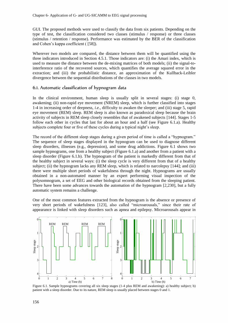
Chapter 6- Application of G- and UG-SICAMM to EEG signal processing
156
GUI. The proposed methods were used to classify the data from six patients. Depending on the
type of test, the classification considered two classes (stimulus / response) or three classes
(stimulus / retention / response). Performance was estimated by the BER of the classification
and Cohen’s kappa coefficient ( [58]).
Wherever two models are compared, the distance between them will be quantified using the
three indicators introduced in Section 4.5.1. Those indicators are: (i) the Amari index, which is
used to measure the distance between the de-mixing matrices of both models; (ii) the signal-to-
interference ratio of the recovered sources, which quantifies the average squared error in the
extraction; and (iii) the probabilistic distance, an approximation of the Kullback-Leibler
divergence between the sequential distributions of the classes in two models.
6.1. Automatic classification of hypnogram data
In the clinical environment, human sleep is usually split in several stages: (i) stage 0,
awakening; (ii) non-rapid eye movement (NREM) sleep, which is further classified into stages
1-4 in increasing order of deepness, i.e., difficulty to awaken the sleeper; and (iii) stage 5, rapid
eye movement (REM) sleep. REM sleep is also known as paradoxical sleep because the brain
activity of subjects in REM sleep closely resembles that of awakened subjects [144]. Stages 1-5
follow each other in cycles that last for about an hour and a half (see Figure 6.1.a). Healthy
subjects complete four or five of these cycles during a typical night’s sleep.
The record of the different sleep stages during a given period of time is called a “hypnogram.”
The sequence of sleep stages displayed in the hypnogram can be used to diagnose different
sleep disorders, illnesses (e.g., depression), and some drug addictions. Figure 6.1 shows two
sample hypnograms, one from a healthy subject (Figure 6.1.a) and another from a patient with a
sleep disorder (Figure 6.1.b). The hypnogram of the patient is markedly different from that of
the healthy subject in several ways: (i) the sleep cycle is very different from that of a healthy
subject; (ii) the hypnogram lacks any REM sleep, which is related to narcolepsy [144]; and (iii)
there were multiple short periods of wakefulness through the night. Hypnograms are usually
obtained in a non-automated manner by an expert performing visual inspection of the
polysomnogram, a set of EEG and other biological records obtained from the sleeping patient.
There have been some advances towards the automation of the hypnogram [2,230], but a fully
automatic system remains a challenge.
One of the most common features extracted from the hypnogram is the absence or presence of
very short periods of wakefulness [123], also called “microarousals,” since their rate of
appearance is linked with sleep disorders such as apnea and epilepsy. Microarousals appear in
Figure 6.1. Sample hypnograms covering all six sleep stages (1-4 plus REM and awakening): a) healthy subject; b)
patient with a sleep disorder. Due to its nature, REM sleep is usually placed between stages 0 and 1.
0 1 2 3 4 5 6 7 8
0
1
2
3
4
a) Time (h)
Sle
ep s
tag
e
REM REM REM REM
0 1 2 3 4 5 6 7
0
1
2
3
4
b) Time (h)
Sle
ep s
tag
e
Automatic classification of hypnogram data
157
the hypnogram as short stays in stage 0, as seen in Figure 6.1.b. In this section, we show a
practical application of the methods proposed in Chapter 4 for automatic detection of
microarousals in real EEG data from apnea patients. The results shown in this section have been
reported in [223,215,221,213].
6.1.1. Data and pre-processing
In this experiment, the proposed methods were applied to perform automatic detection of
microarousals. Hence, the classification will only consider two classes: (i) class 1, which
corresponds to any stage of actual sleep (NREM and REM); and (ii) class 2, which corresponds
to microarousals (i.e., stage 0 from the hypnogram). Six 8-hour records were considered for the
experiment, each from a different apnea patient. The records and their respective reference
hypnograms were obtained by an expert using conventional, non-automated, procedures. As in
Section 4.5.3, the results of SICAMM and its variants will be compared against those of
ICAMM and several types of Bayesian networks. These automatic classifications will be
compared with the non-automated classifications made by the expert, which we will assume to
be the ground truth.
The recorded PSG were composed by 24 channels each, 11 EEG channels and 13 other channels
measuring muscle signals, breathing, and other physiological characteristics. For this
experiment, however, only the EEG channels were considered. The 11 EEG channels were
sampled at 256 Hz, band-pass filtered using a Butterworth filter of order 6 between 0.2 and 70
Hz, and then a notch filter at 50 Hz was used to remove line noise. The filtered signals were
split in 1-3 seconds long epochs (256 to 768 samples) without overlapping, and four features
were calculated at each epoch. These features where then averaged for 30-second segments,
which were used by the proposed methods for training and testing. Thus, a decision about the
sleep stage of the subject is taken every 30 seconds.
6.1.1.a. Extracted features
The four features extracted from the PSG signals were: amplitude, dominant rhythm (centroid
frequency), and theta-slow-wave index (TSI) from channel C3-A2; and alpha-slow-wave index
(ASI) from EEG channel O2-A1. These features are commonly used in PSG analysis [2,123],
and their definitions are included in the following.
Average amplitude
The average amplitude is the average absolute value of the voltage at every electrode during an
epoch. It was calculated as the sample average of the absolute value of the EEG signal; thus, the
average amplitude of the -thi channel is
1
1N
i i
n
x x nN
(6.1)
where ix n are the data from the -thi channel 1, ..., 6 4i at time sample n , and with each
epoch being N samples long ( N ranged from 256 to 768 samples).
Centroid frequency
The centroid frequency is the “center of gravity” of the frequency transform of the data from
every channel during an epoch. It was calculated as the frequency of the first pole of the AR
model,

Chapter 6- Application of G- and UG-SICAMM to EEG signal processing
158
1
p
i j i
j
x n w x n j
(6.2)
where , 1, ... ,j
w j p , are the parameters of the AR model. In this work, a second-order model
2p was considered. This method of calculation of the centroid frequency is common in
sleep staging [2].
Alpha Slow-wave Index (ASI)
The ASI is the ratio of power in the alpha band (8-11 Hz) with respect to the power in the delta
and theta band (0.5-3.5 Hz and 3.5-8 Hz, respectively):
,
, ,
A S I a t ch an n e l :i a lp h a
i
i d e lta i th e ta
Pi A S I
P P
(6.3)
where ,i a lp h a
P is the power at the -thi channel during the epoch, considering only the power at
the frequencies within the alpha band; and , ,
,i d e l ta i th e ta
P P are defined likewise.
Theta Slow-wave Index (TSI)
The TSI is the ratio of power in the theta band with respect the power in both the alpha and the
delta bands:
,
, ,
T S I a t ch an n e l :i th e ta
i
i d e lta i a lp h a
Pi T S I
P P
(6.4)
6.1.1.b. Estimation of SICAMM parameters
The first half of the data was used to estimate the parameters of each method (ICAMM,
SICAMM and Bayesian networks) in a supervised form, considering the labels provided by the
expert. Due to the low number of features, G-SICAMM was not used. The ICAMM parameters,
, ,k k k
pW s b , were estimated from the training record by the JADE algorithm ( [231])
embedded in the MIXCA procedure. The transition probabilities between classes were also
estimated from the training record, and they are shown in Table 6.1. Note that all the
probabilities of permanence in the same class are clearly above 0.5, justifying the use of
sequential dependence in this application.
Subject 1 Subject 2 Subject 3
Class 1 Class 2 Class 1 Class 2 Class 1 Class 2
Class 1 0.98 0.02 Class 1 0.96 0.04 Class 1 0.97 0.03
Class 2 0.31 0.69 Class 2 0.20 0.80 Class 2 0.06 0.94
Subject 4 Subject 5 Subject 6
Class 1 Class 2 Class 1 Class 2 Class 1 Class 2
Class 1 0.91 0.09 Class 1 0.97 0.03 Class 1 0.99 0.01
Class 2 0.31 0.69 Class 2 0.21 0.79 Class 2 0.14 0.86 Table 6.1. Estimated transition probabilities for the studied subjects.
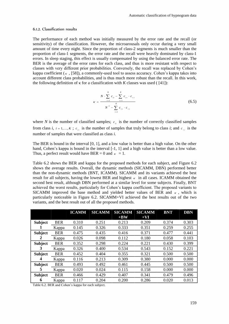
Automatic classification of hypnogram data
159
6.1.2. Classification results
The performance of each method was initially measured by the error rate and the recall (or
sensitivity) of the classification. However, the microarousals only occur during a very small
amount of time every night. Since the proportion of class-2 segments is much smaller than the
proportion of class-1 segments, the error rate and the recall were heavily dominated by class-1
errors. In sleep staging, this effect is usually compensated by using the balanced error rate. The
BER is the average of the error rates for each class, and thus is more resistant with respect to
classes with very different prior probabilities. Conversely, the recall was replaced by Cohen’s
kappa coefficient ( , [58]), a commonly-used tool to assess accuracy. Cohen’s kappa takes into
account different class probabilities, and is thus much more robust than the recall. In this work,
the following definition of κ for a classification with K classes was used ( [41]):
1 1
2
1
K K
ii i i
i i
K
i i
i
N c c c
N c c
(6.5)
where N is the number of classified samples; i i
c is the number of correctly classified samples
from class i, 1, ...,i K ; i
c
is the number of samples that truly belong to class i; and i
c
is the
number of samples that were classified as class i.
The BER is bound in the interval [0, 1], and a low value is better than a high value. On the other
hand, Cohen’s kappa is bound in the interval [-1, 1] and a high value is better than a low value.
Thus, a perfect result would have BER = 0 and = 1.
Table 6.2 shows the BER and kappa for the proposed methods for each subject, and Figure 6.2
shows the average results. Overall, the dynamic methods (SICAMM, DBN) performed better
than the non-dynamic methods (BNT, ICAMM). SICAMM and its variants achieved the best
result for all subjects, having the lowest BER and highest in all cases. ICAMM obtained the
second best result, although DBN performed at a similar level for some subjects. Finally, BNT
achieved the worst results, particularly for Cohen’s kappa coefficient. The proposed variants to
SICAMM improved the base method and yielded better values of BER and , which is
particularly noticeable in Figure 6.2. SICAMM+VI achieved the best results out of the two
variants, and the best result out of all the proposed methods.
ICAMM SICAMM SICAMM
+BW
SICAMM
+VI
BNT DBN
Subject
1
BER 0.310 0.251 0.213 0.209 0.374 0.303
Kappa 0.145 0.326 0.333 0.351 0.259 0.255
Subject
2
BER 0.475 0.435 0.416 0.371 0.477 0.441
Kappa 0.026 0.098 0.112 0.180 0.058 0.103
Subject
3
BER 0.352 0.298 0.224 0.221 0.430 0.399
Kappa 0.326 0.400 0.534 0.543 0.152 0.221
Subject
4
BER 0.452 0.404 0.355 0.321 0.500 0.500
Kappa 0.116 0.213 0.309 0.380 0.000 0.000
Subject
5
BER 0.493 0.492 0.461 0.445 0.500 0.500
Kappa 0.020 0.024 0.115 0.158 0.000 0.000
Subject
6
BER 0.466 0.429 0.407 0.341 0.479 0.496
Kappa 0.117 0.204 0.200 0.286 0.020 0.013 Table 6.2. BER and Cohen’s kappa for each subject.
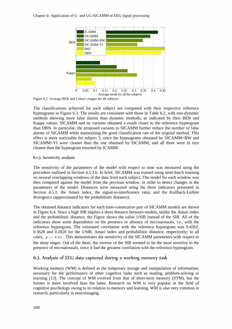
Chapter 6- Application of G- and UG-SICAMM to EEG signal processing
160
Figure 6.2. Average BER and Cohen’s kappa for all subjects.
The classifications achieved for each subject are compared with their respective reference
hypnograms in Figure 6.3. The results are consistent with those in Table 6.2, with non-dynamic
methods showing more false alarms than dynamic methods, as indicated by their BER and
Kappa values. SICAMM and its variants obtained a result closer to the reference hypnogram
than DBN. In particular, the proposed variants to SICAMM further reduce the number of false
alarms of SICAMM while maintaining the good classification rate of the original method. This
effect is more noticeable for subject 3, since the hypnograms obtained by SICAMM+BW and
SICAMM+VI were cleaner than the one obtained by SICAMM, and all three were in turn
cleaner than the hypnogram returned by ICAMM.
6.1.3. Sensitivity analysis
The sensitivity of the parameters of the model with respect to time was measured using the
procedure outlined in Section 4.5.3.b. In brief, SICAMM was trained using semi-batch learning
on several overlapping windows of the data from each subject. The model for each window was
then compared against the model from the previous window, in order to detect changes in the
parameters of the model. Distances were measured using the three indicators presented in
Section 4.5.1: the Amari index, the signal-to-interference ratio, and the Kullback-Leibler
divergence (approximated by the probabilistic distance).
The obtained distance indicators for each time-consecutive pair of SICAMM models are shown
in Figure 6.4. Since a high SIR implies a short distance between models, unlike the Amari index
and the probabilistic distance, the Figure shows the value 1/SIR instead of the SIR. All of the
indicators show some dependence on the presence or absence of microarousals, i.e., with the
reference hypnogram. The estimated correlation with the reference hypnogram was 0.4362,
0.3628 and 0.2828 for the 1/SIR, Amari index and probabilistic distance, respectively; in all
cases, 0 .0 5p . This demonstrates the sensitivity of the SICAMM parameters with respect to
the sleep stages. Out of the three, the inverse of the SIR seemed to be the most sensitive to the
presence of microarousals, since it had the greatest correlation with the reference hypnogram.
6.2. Analysis of EEG data captured during a working memory task
Working memory (WM) is defined as the temporary storage and manipulation of information,
necessary for the performance of other cognitive tasks such as reading, problem-solving or
learning [13]. The concept of WM evolved from that of short-term memory (STM), but the
former is more involved than the latter. Research on WM is very popular in the field of
cognitive psychology owing to its relation to memory and learning. WM is also very common in
research, particularly in neuroimaging.
0 0.05 0.1 0.15 0.2 0.25 0.3 0.35 0.4 0.45
BER
Kappa
Average result for all the subjects
ICAMM
SICAMM
SICAMM+BW
SICAMM+VI
BNT
DBN
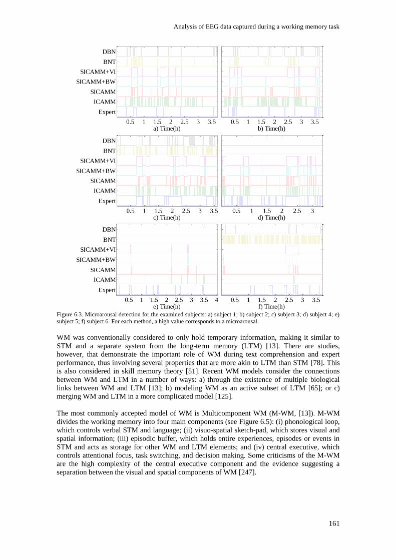
Analysis of EEG data captured during a working memory task
161
Figure 6.3. Microarousal detection for the examined subjects: a) subject 1; b) subject 2; c) subject 3; d) subject 4; e)
subject 5; f) subject 6. For each method, a high value corresponds to a microarousal.
WM was conventionally considered to only hold temporary information, making it similar to
STM and a separate system from the long-term memory (LTM) [13]. There are studies,
however, that demonstrate the important role of WM during text comprehension and expert
performance, thus involving several properties that are more akin to LTM than STM [78]. This
is also considered in skill memory theory [51]. Recent WM models consider the connections
between WM and LTM in a number of ways: a) through the existence of multiple biological
links between WM and LTM [13]; b) modeling WM as an active subset of LTM [65]; or c)
merging WM and LTM in a more complicated model [125].
The most commonly accepted model of WM is Multicomponent WM (M-WM, [13]). M-WM
divides the working memory into four main components (see Figure 6.5): (i) phonological loop,
which controls verbal STM and language; (ii) visuo-spatial sketch-pad, which stores visual and
spatial information; (iii) episodic buffer, which holds entire experiences, episodes or events in
STM and acts as storage for other WM and LTM elements; and (iv) central executive, which
controls attentional focus, task switching, and decision making. Some criticisms of the M-WM
are the high complexity of the central executive component and the evidence suggesting a
separation between the visual and spatial components of WM [247].
0.5 1 1.5 2 2.5 3 3.5
Expert
ICAMM
SICAMM
SICAMM+BW
SICAMM+VI
BNT
DBN
a) Time(h)0.5 1 1.5 2 2.5 3 3.5
b) Time(h)
0.5 1 1.5 2 2.5 3 3.5
Expert
ICAMM
SICAMM
SICAMM+BW
SICAMM+VI
BNT
DBN
c) Time(h)0.5 1 1.5 2 2.5 3
d) Time(h)
0.5 1 1.5 2 2.5 3 3.5 4
Expert
ICAMM
SICAMM
SICAMM+BW
SICAMM+VI
BNT
DBN
e) Time(h)0.5 1 1.5 2 2.5 3 3.5
f) Time(h)
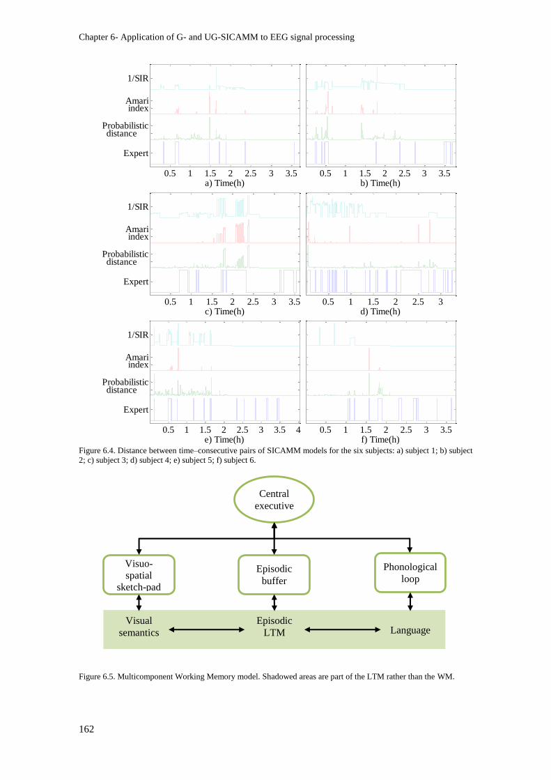
Chapter 6- Application of G- and UG-SICAMM to EEG signal processing
162
Figure 6.4. Distance between time–consecutive pairs of SICAMM models for the six subjects: a) subject 1; b) subject
2; c) subject 3; d) subject 4; e) subject 5; f) subject 6.
Figure 6.5. Multicomponent Working Memory model. Shadowed areas are part of the LTM rather than the WM.
0.5 1 1.5 2 2.5 3 3.5
Expert
distance Probabilistic
indexAmari
1/SIR
a) Time(h)0.5 1 1.5 2 2.5 3 3.5
b) Time(h)
0.5 1 1.5 2 2.5 3 3.5
Expert
distance Probabilistic
indexAmari
1/SIR
c) Time(h)0.5 1 1.5 2 2.5 3
d) Time(h)
0.5 1 1.5 2 2.5 3 3.5 4
Expert
distance Probabilistic
indexAmari
1/SIR
e) Time(h)0.5 1 1.5 2 2.5 3 3.5
f) Time(h)
Central
executive
Visuo-
spatial
sketch-pad
Episodic
buffer
Phonological
loop
Visual
semantics
Episodic
LTM Language

Analysis of EEG data captured during a working memory task
163
Working memory and cognitive control functions have been associated most commonly with
the prefrontal cortex (PFC) [34]. This idea is supported by PET studies that have shown
activation of this region during a variety of cognitively demanding tasks, all of which can be
thought to invoke short-term working memory. These tasks seem to activate similar regions of
the PFC despite the fact that different types of information are involved. However, fMRI studies
show that other areas do activate during WM tasks, particularly in prefrontal and parietal areas
[34]. The fMRI studies provide more precise location, determining areas that relate to different
WM tasks [272].
Studies on working memory test the subjects with different cognitive tasks. In this experiment,
the subjects were performing the Sternberg memory task [251], one of the most well-known
working memory tests. The Sternberg memory task was introduced in Section 5.4.2.
6.2.1. Experiment configuration
The data processing for this experiment can be split into a series of stages or modules, as shown
in Figure 6.6. The process initiates with the capture of electroencephalographic data while the
subject performs a working memory task. Once captured, data are pre-processed to remove
noise and extract several features from them. These extracted features are used for data labeling
by determining the activity of each hemisphere at each particular time sample. After the labels
are calculated, the parameters of each method are estimated from the first half of the data. These
parameters are used afterward to classify the second half of the data, i.e., to attempt to
automatically determine the level of brain activity in each hemisphere. Finally, these
classifications are compared against the previously-estimated labels to test the classification
performance of our system. Each of these stages will be studied in depth in the following
sections.
Figure 6.6. Diagram of the EEG data processing stages.
6.2.1.a. Data capture and EEG signal pre-processing
The data capture process was the same that was explained in Section 5.4.1. The captured signals
were filtered to remove noise caused both by the environment and by the capture device. The
filters are explained in Section 5.4.1 as well, and the locations of each one of the 64 electrodes
is shown in Figure 5.19. After filtering, data are split into data segments of a short duration,
known as epochs, to obtain local estimates of the features and improve the classification.
Epochs were windowed prior to feature extraction to avoid high-frequency artifacts caused by
the artificial separation of the data, attenuating the values of all channels at the beginning and
Capture EEG data from subjects
•Pre-process data
Estimate labels from data
Estimate models
• Train using first half of data
• Classify second half of data
Calculate performance

Chapter 6- Application of G- and UG-SICAMM to EEG signal processing
164
the end of the epoch. For this application, we considered epochs of length 0.1 seconds, which
corresponds to 205 samples, and Hamming windows. Each epoch is treated as a separate
observation with respect to the models and classifiers. Thus, a decision on the state of the
subject was taken every 0.1 seconds.
6.2.1.b. Feature extraction
Twelve features were extracted from each epoch of the EEG data (see Table 6.3), and each was
calculated separately for each channel and for each epoch. The features are explained in detail
below. Note that the average amplitude, the centroid frequency, the TSI and the ASI were
already introduced in Section 6.1.1.a.
Kind of feature Feature
Amplitude Average amplitude
Maximum amplitude
Average power
Spectral Centroid frequency
Peak frequency
Spindles ratio
TSI
ASI
Statistical Skewness
Kurtosis
Time reversibility
Third-order autocovariance Table 6.3. List of features calculated from each epoch.
Maximum amplitude
The maximum amplitude is the maximum absolute value of the voltage at every electrode
during an epoch. It was calculated as
m ax im u m am p litu d e a t ch an n el : m ax , 1, ...,M A X
i ii x x n n N (6.6)
Average power
The average power is the average quadratic value of the EEG signal during an epoch. It is
calculated as
2
1
1av e rag e p o w er a t ch an n e l :
N
i i
n
i P x nN
(6.7)
Peak frequency
The peak frequency is the frequency which concentrates the maximum amount of energy in
each channel for an epoch. Note that it is not necessarily equal to the centroid frequency, since
the maximum frequency only searches for the energy at a single frequency, while the centroid
frequency considers all points of the frequency spectrum. It is calculated as
2
p eak freq u en cy: m axM A X
i i
f
f X f (6.8)
where iX f is the frequency spectrum of the -thi channel.

Analysis of EEG data captured during a working memory task
165
Spindles ratio
Spindles are oscillatory bursts of brain activity in the sigma band (11.5-15 Hz). The spindles
ratio is calculated as the ratio of power in the sigma band with respect to the power of the other
EEG bands:
,
,
S p in d les ra tio a t ch an n e l :i s ig m a
i
i i s ig m a
Pi IS
P P
(6.9)
where ,i s ig m a
P is the average power of the -thi channel during the epoch, considering only the
power at the frequencies within the sigma band.
Skewness
The skewness or asymmetry is a statistical indicator of how asymmetrical a probability density
function is with respect to its mean. A skewness close to zero indicates a symmetrical PDF,
while a skewness far from zero (be it negative or positive) indicates an asymmetrical PDF. It is
calculated as
3
1, 3
1
1S k ew n ess a t ch an n e l :
Ni i
i
n i
x n xi
N
(6.10)
where i
is the standard deviation at the -thi channel.
Kurtosis
Kurtosis is a statistical indicator of how “peaked” a probability density function is. It is usually
normalized with respect to a Gaussian distribution, which corresponds to an un-normalized
kurtosis of 3. A PDF that is very sharp around its mean, but shows very long tails, will have a
kurtosis greater than that of a Gaussian distribution; it is known as “super-Gaussian”.
Conversely, a distribution that is smoother around its mean, with smaller tails, will have a
kurtosis lower than that of a Gaussian distribution and be known as “sub-Gausian”. It is
calculated as
4
2 , 4
1
1K u rto s is a t ch an n e l : 3
Ni i
i
n i
x n xi
N
(6.11)
where the 3 is a normalization factor, and is equal to the kurtosis of a Gaussian distribution.
Time reversibility
The time reversibility of a signal is an indicator of how symmetrical with respect to time is the
signal in each channel during an epoch. A symmetrical signal has time reversibility equal to
zero, and an asymmetrical signal has larger time reversibility. It is calculated as
3
3
1
1 1T im e re v e rs ib ili ty a t c h a n n e l :
N
i i i
ni
i T R E V x n x nN
(6.12)
where is the considered lag (in this work, 1 ).
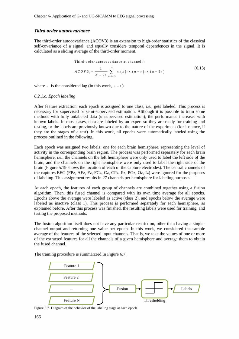
Chapter 6- Application of G- and UG-SICAMM to EEG signal processing
166
Third-order autocovariance
The third-order autocovariance (ACOV3) is an extension to high-order statistics of the classical
self-covariance of a signal, and equally considers temporal dependences in the signal. It is
calculated as a sliding average of the third-order moment,
1 2
T h ird -o rd e r a u to c o v a ria n c e a t c h a n n e l :
13 2
2
N
i i i i
n
i
A C O V x n x n x nN
(6.13)
where is the considered lag (in this work, 1 ).
6.2.1.c. Epoch labeling
After feature extraction, each epoch is assigned to one class, i.e., gets labeled. This process is
necessary for supervised or semi-supervised estimation. Although it is possible to train some
methods with fully unlabeled data (unsupervised estimation), the performance increases with
known labels. In most cases, data are labeled by an expert so they are ready for training and
testing, or the labels are previously known due to the nature of the experiment (for instance, if
they are the stages of a test). In this work, all epochs were automatically labeled using the
process outlined in the following.
Each epoch was assigned two labels, one for each brain hemisphere, representing the level of
activity in the corresponding brain region. The process was performed separately for each brain
hemisphere, i.e., the channels on the left hemisphere were only used to label the left side of the
brain, and the channels on the right hemisphere were only used to label the right side of the
brain (Figure 5.19 shows the location of each of the capture electrodes). The central channels of
the captures EEG (FPz, AFz, Fz, FCz, Cz, CPz, Pz, POz, Oz, Iz) were ignored for the purposes
of labeling. This assignment results in 27 channels per hemisphere for labeling purposes.
At each epoch, the features of each group of channels are combined together using a fusion
algorithm. Then, this fused channel is compared with its own time average for all epochs.
Epochs above the average were labeled as active (class 2), and epochs below the average were
labeled as inactive (class 1). This process is performed separately for each hemisphere, as
explained before. After this process was finished, the resulting labels were used for training, and
testing the proposed methods.
The fusion algorithm itself does not have any particular restriction, other than having a single-
channel output and returning one value per epoch. In this work, we considered the sample
average of the features of the selected input channels. That is, we take the values of one or more
of the extracted features for all the channels of a given hemisphere and average them to obtain
the fused channel.
The training procedure is summarized in Figure 6.7.
Figure 6.7. Diagram of the behavior of the labeling stage at each epoch.
Feature 1
Feature 2
... Fusion
Thresholding
Labels
Feature N
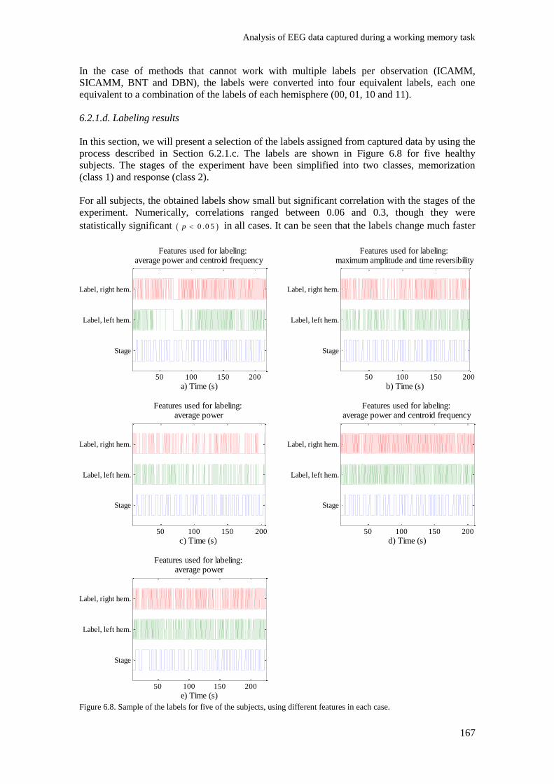
Analysis of EEG data captured during a working memory task
167
In the case of methods that cannot work with multiple labels per observation (ICAMM,
SICAMM, BNT and DBN), the labels were converted into four equivalent labels, each one
equivalent to a combination of the labels of each hemisphere (00, 01, 10 and 11).
6.2.1.d. Labeling results
In this section, we will present a selection of the labels assigned from captured data by using the
process described in Section 6.2.1.c. The labels are shown in Figure 6.8 for five healthy
subjects. The stages of the experiment have been simplified into two classes, memorization
(class 1) and response (class 2).
For all subjects, the obtained labels show small but significant correlation with the stages of the
experiment. Numerically, correlations ranged between 0.06 and 0.3, though they were
statistically significant 0 .0 5p in all cases. It can be seen that the labels change much faster
Figure 6.8. Sample of the labels for five of the subjects, using different features in each case.
50 100 150 200
Stage
Label, left hem.
Label, right hem.
Features used for labeling: average power and centroid frequency
a) Time (s)50 100 150 200
Stage
Label, left hem.
Label, right hem.
Features used for labeling: maximum amplitude and time reversibility
b) Time (s)
50 100 150 200
Stage
Label, left hem.
Label, right hem.
Features used for labeling: average power
c) Time (s)50 100 150 200
Stage
Label, left hem.
Label, right hem.
Features used for labeling: average power and centroid frequency
d) Time (s)
50 100 150 200
Stage
Label, left hem.
Label, right hem.
Features used for labeling: average power
e) Time (s)

Chapter 6- Application of G- and UG-SICAMM to EEG signal processing
168
Figure 6.9. Detail of the labels for one of the subjects (subject from Figure 6.8.b).
than the stages of the experiment but are still correlated with them, as shown in Figure 6.9. This
faster variation persists even if we change the fusion algorithm or the threshold, and even if we
change the features selected for labeling.
6.2.1.e. Training and testing
The EEG data of each subject were split into two sets. The central 30% of the data was used for
training, and the remaining 70% was used for testing the classification performance of the
proposed methods (see Figure 6.10). The selection of the central 30% of the data was done so as
to minimize any possible difference caused by a lack of concentration of the subject at the
beginning or at the end of the experiment.
Figure 6.10. Diagram of the data split into classification and testing sets.
As in the case of the labeling process, the system can use one or more of the extracted features
in order to classify data. If more than one feature is selected, the system considers the features
as extra channels. Note that the features selected for training and for classification must be the
same, but can be different from the ones selected for labeling.
For the methods with two chains (G-SICAMM and DBN2), the channels from each feature were
separated according to their hemisphere. The channels from the left side of the brain were
assigned to the left hemisphere and channels from the right side of the brain were assigned to
the right hemisphere. Central channels (FPz, AFz, Fz, FCz, Cz, CPz, Pz, POz, Oz, Iz) were
ignored with respect to data training and classification. Thus, G-SICAMM and DBN2
considered 27 channels per hemisphere. The rest of the proposed methods worked with all 64
channels.
Once training and classification data were selected, we performed PCA on the selected features
[124]. The number of components to keep, 'M , was estimated so the sum of the explained
variances of the selected components was at least 95% of the total variance in the original data.
This selection means that the number of components changes depending on the subject, as well
as the number of selected features for training and testing. In the case of methods with two
chains (G-SICAMM and DBN2), since they have different datasets for each hemisphere, a
different PCA was calculated for each hemisphere.
65 70 75 80 85 90
Stage
Label, left hem.
Label, right hem.
Features used for labeling: maximum amplitude and time reversibility
Time (s)
Classification Training Classification

Analysis of EEG data captured during a working memory task
169
The parameters for each of the proposed methods were estimated as follows. G-SICAMM was
with two chains and two classes per chain (K = 2 and L = 2). For the SICAMM and ICAMM, a
single model was fitted for the data from both hemispheres, that is, the model is fit to
1 2,
TT T
n n n
x x x . As explained in Section 6.2.1.c, in order to compare these models
with the one obtained with G-SICAMM, SICAMM and ICAMM considered four classes (K =
4), one class per combination of classes from each chain (both hemispheres inactive, left
hemisphere active, right hemisphere active, and both hemispheres active). In all cases,
parameter estimation was performed with supervised training using the estimated labels with the
JADE algorithm ( [231]) embedded in the MIXCA procedure.
The configuration of the dynamic Bayesian network was dynamically adjusted to the data.
Three types of DBN were considered, each one similar to one of the ICA-based methods: a
network without temporal dependence (BNT), a single network with a HMM (DBN1), and a
network with a two-chain CHMM (DBN2). The configuration of these methods was similar to
that of the ICAMM-based methods: for the DBN2, two chains were considered, each one with
two states (K = 2 and L = 2); and DBN1 and BNT were adjusted considering four states, K = 4.
Node probabilities were modeled using a Gaussian Mixture Model (GMM) with a variable
number of mixtures for each node. The number of mixtures for each node was determined by
testing several GMM with an increasing number of classes (3 to 20) and choosing the model
with a lower Akaike Information Criterion. In this work, most GMM ended up with seven to ten
components.
6.2.2. Classification results
The performance of the classification of the state of each brain hemisphere can be evaluated in
one of two ways. The first would be to determine the number of samples which are correctly
classified for both hemispheres at the same time. In practice, this is a classification problem
with four classes, since there are four possibilities: (i) both hemispheres inactive; (ii) left active
and right inactive; (iii) left inactive and right active; and (iv) both hemispheres active. However,
the performance of the classification could also be evaluated separately for each hemisphere,
i.e., counting how many times has a hemisphere been correctly classified as active or inactive.
This second case is thus a two-class classification case. This Section explores both evaluations
of the performance of each classification.
Regardless of the number of classes, classification performance is usually estimated from their
confusion matrix (or error matrix), a matrix defined such that its element (i, j) is equal to the
number of observations that truly belong to class i and have been labeled as class j by the
method. A good classifier should have a diagonal or close-to-diagonal confusion matrix. Table
6.4 and Table 6.5 show two examples of confusion matrices for four-class and two-class
classification, respectively. Note the largely uneven distribution of the true classes. For instance,
the case shown in Table 6.4 had 1483 values that belonged to class 00 (both hemispheres
inactive), but only 112 that belonged to class 11 (both hemispheres active). Therefore, the
performance of the classification was estimated with the balanced error rate, an indicator that is
robust with respect to differences in class probability.
Table 6.6 shows the BER of the four-class classification obtained by each of the proposed
methods. To unify results, all subjects were labeled using the same feature (average power) and
classified using the same two features (centroid frequency and spindles ratio). Although the
BER is somewhat large, note that the average BER of a trivial classifier would be 75% because
of the four classes. Out of all the proposed methods, only SICAMM, G-SICAMM and their
variants performed significantly better than the base performance. G-SICAMM+VI achieved the
best result, an average BER of 54.49% across all subjects. Overall, dynamic methods yielded
better results than non-dynamic methods.
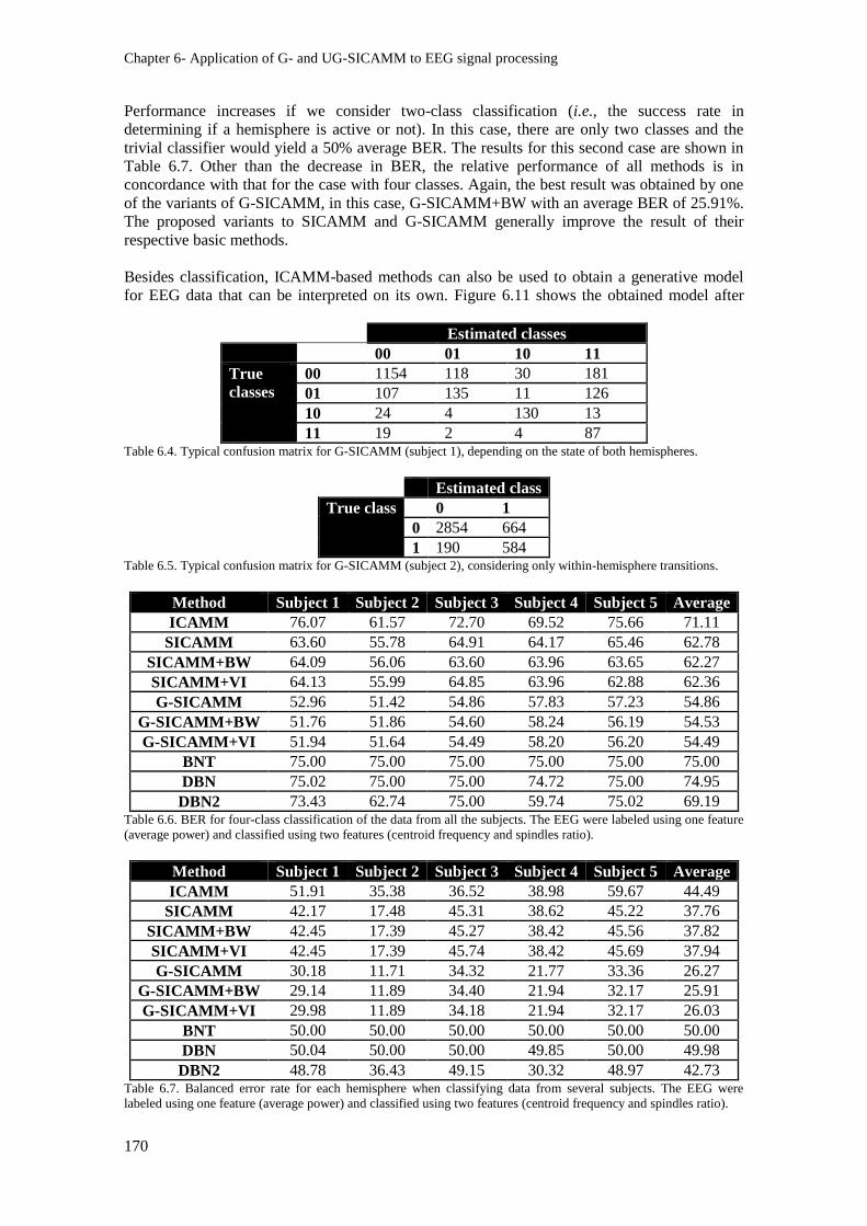
Chapter 6- Application of G- and UG-SICAMM to EEG signal processing
170
Performance increases if we consider two-class classification (i.e., the success rate in
determining if a hemisphere is active or not). In this case, there are only two classes and the
trivial classifier would yield a 50% average BER. The results for this second case are shown in
Table 6.7. Other than the decrease in BER, the relative performance of all methods is in
concordance with that for the case with four classes. Again, the best result was obtained by one
of the variants of G-SICAMM, in this case, G-SICAMM+BW with an average BER of 25.91%.
The proposed variants to SICAMM and G-SICAMM generally improve the result of their
respective basic methods.
Besides classification, ICAMM-based methods can also be used to obtain a generative model
for EEG data that can be interpreted on its own. Figure 6.11 shows the obtained model after
Estimated classes
00 01 10 11
True
classes
00 1154 118 30 181
01 107 135 11 126
10 24 4 130 13
11 19 2 4 87 Table 6.4. Typical confusion matrix for G-SICAMM (subject 1), depending on the state of both hemispheres.
Estimated class
True class 0 1
0 2854 664
1 190 584 Table 6.5. Typical confusion matrix for G-SICAMM (subject 2), considering only within-hemisphere transitions.
Method Subject 1 Subject 2 Subject 3 Subject 4 Subject 5 Average
ICAMM 76.07 61.57 72.70 69.52 75.66 71.11
SICAMM 63.60 55.78 64.91 64.17 65.46 62.78
SICAMM+BW 64.09 56.06 63.60 63.96 63.65 62.27
SICAMM+VI 64.13 55.99 64.85 63.96 62.88 62.36
G-SICAMM 52.96 51.42 54.86 57.83 57.23 54.86
G-SICAMM+BW 51.76 51.86 54.60 58.24 56.19 54.53
G-SICAMM+VI 51.94 51.64 54.49 58.20 56.20 54.49
BNT 75.00 75.00 75.00 75.00 75.00 75.00
DBN 75.02 75.00 75.00 74.72 75.00 74.95
DBN2 73.43 62.74 75.00 59.74 75.02 69.19 Table 6.6. BER for four-class classification of the data from all the subjects. The EEG were labeled using one feature
(average power) and classified using two features (centroid frequency and spindles ratio).
Method Subject 1 Subject 2 Subject 3 Subject 4 Subject 5 Average
ICAMM 51.91 35.38 36.52 38.98 59.67 44.49
SICAMM 42.17 17.48 45.31 38.62 45.22 37.76
SICAMM+BW 42.45 17.39 45.27 38.42 45.56 37.82
SICAMM+VI 42.45 17.39 45.74 38.42 45.69 37.94
G-SICAMM 30.18 11.71 34.32 21.77 33.36 26.27
G-SICAMM+BW 29.14 11.89 34.40 21.94 32.17 25.91
G-SICAMM+VI 29.98 11.89 34.18 21.94 32.17 26.03
BNT 50.00 50.00 50.00 50.00 50.00 50.00
DBN 50.04 50.00 50.00 49.85 50.00 49.98
DBN2 48.78 36.43 49.15 30.32 48.97 42.73 Table 6.7. Balanced error rate for each hemisphere when classifying data from several subjects. The EEG were
labeled using one feature (average power) and classified using two features (centroid frequency and spindles ratio).
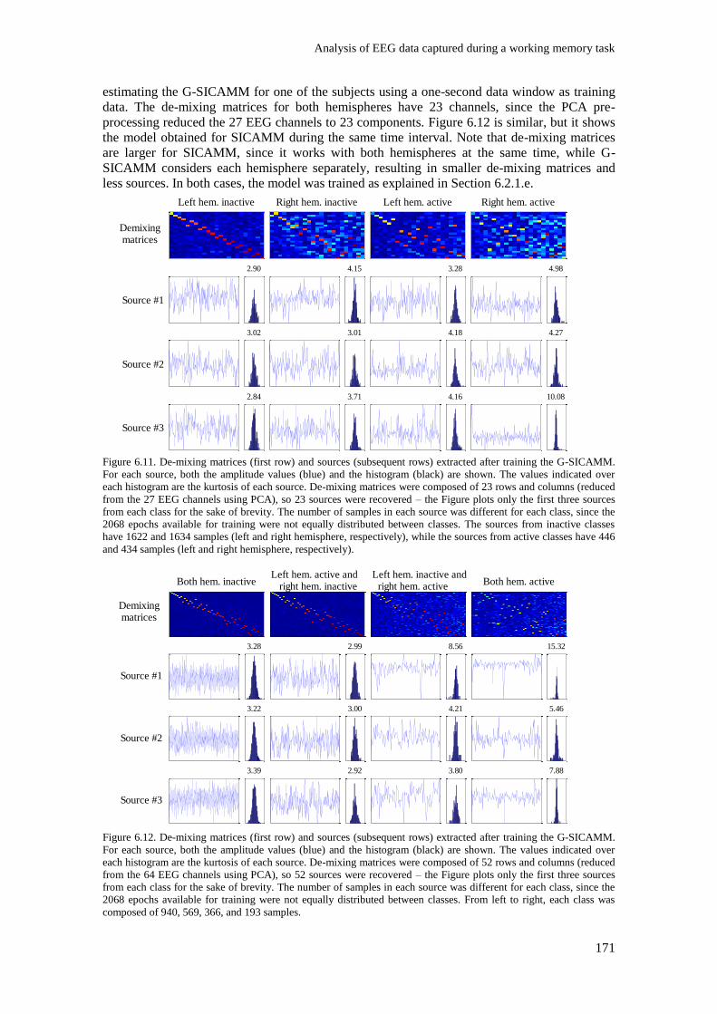
Analysis of EEG data captured during a working memory task
171
estimating the G-SICAMM for one of the subjects using a one-second data window as training
data. The de-mixing matrices for both hemispheres have 23 channels, since the PCA pre-
processing reduced the 27 EEG channels to 23 components. Figure 6.12 is similar, but it shows
the model obtained for SICAMM during the same time interval. Note that de-mixing matrices
are larger for SICAMM, since it works with both hemispheres at the same time, while G-
SICAMM considers each hemisphere separately, resulting in smaller de-mixing matrices and
less sources. In both cases, the model was trained as explained in Section 6.2.1.e.
Figure 6.11. De-mixing matrices (first row) and sources (subsequent rows) extracted after training the G-SICAMM.
For each source, both the amplitude values (blue) and the histogram (black) are shown. The values indicated over
each histogram are the kurtosis of each source. De-mixing matrices were composed of 23 rows and columns (reduced
from the 27 EEG channels using PCA), so 23 sources were recovered – the Figure plots only the first three sources
from each class for the sake of brevity. The number of samples in each source was different for each class, since the
2068 epochs available for training were not equally distributed between classes. The sources from inactive classes
have 1622 and 1634 samples (left and right hemisphere, respectively), while the sources from active classes have 446
and 434 samples (left and right hemisphere, respectively).
Figure 6.12. De-mixing matrices (first row) and sources (subsequent rows) extracted after training the G-SICAMM.
For each source, both the amplitude values (blue) and the histogram (black) are shown. The values indicated over
each histogram are the kurtosis of each source. De-mixing matrices were composed of 52 rows and columns (reduced
from the 64 EEG channels using PCA), so 52 sources were recovered – the Figure plots only the first three sources
from each class for the sake of brevity. The number of samples in each source was different for each class, since the
2068 epochs available for training were not equally distributed between classes. From left to right, each class was
composed of 940, 569, 366, and 193 samples.
Left hem. inactive
Demixing matrices
Right hem. inactive Left hem. active Right hem. active
Source #1
2.90 4.15 3.28 4.98
Source #2
3.02 3.01 4.18 4.27
Source #3
2.84 3.71 4.16 10.08
Both hem. inactive
Demixing matrices
Left hem. active and right hem. inactive
Left hem. inactive andright hem. active
Both hem. active
Source #1
3.28 2.99 8.56 15.32
Source #2
3.22 3.00 4.21 5.46
Source #3
3.39 2.92 3.80 7.88
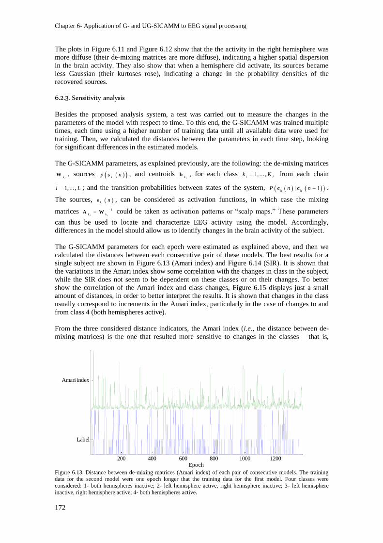
Chapter 6- Application of G- and UG-SICAMM to EEG signal processing
172
The plots in Figure 6.11 and Figure 6.12 show that the the activity in the right hemisphere was
more diffuse (their de-mixing matrices are more diffuse), indicating a higher spatial dispersion
in the brain activity. They also show that when a hemisphere did activate, its sources became
less Gaussian (their kurtoses rose), indicating a change in the probability densities of the
recovered sources.
6.2.3. Sensitivity analysis
Besides the proposed analysis system, a test was carried out to measure the changes in the
parameters of the model with respect to time. To this end, the G-SICAMM was trained multiple
times, each time using a higher number of training data until all available data were used for
training. Then, we calculated the distances between the parameters in each time step, looking
for significant differences in the estimated models.
The G-SICAMM parameters, as explained previously, are the following: the de-mixing matrices
lk
W , sources l
kp ns , and centroids
lk
b , for each class 1, ...,l l
k K from each chain
1, ...,l L ; and the transition probabilities between states of the system, | 1P n n k k'
c c .
The sources, l
kns , can be considered as activation functions, in which case the mixing
matrices 1
l lk k
A W could be taken as activation patterns or “scalp maps.” These parameters
can thus be used to locate and characterize EEG activity using the model. Accordingly,
differences in the model should allow us to identify changes in the brain activity of the subject.
The G-SICAMM parameters for each epoch were estimated as explained above, and then we
calculated the distances between each consecutive pair of these models. The best results for a
single subject are shown in Figure 6.13 (Amari index) and Figure 6.14 (SIR). It is shown that
the variations in the Amari index show some correlation with the changes in class in the subject,
while the SIR does not seem to be dependent on these classes or on their changes. To better
show the correlation of the Amari index and class changes, Figure 6.15 displays just a small
amount of distances, in order to better interpret the results. It is shown that changes in the class
usually correspond to increments in the Amari index, particularly in the case of changes to and
from class 4 (both hemispheres active).
From the three considered distance indicators, the Amari index (i.e., the distance between de-
mixing matrices) is the one that resulted more sensitive to changes in the classes – that is,
Figure 6.13. Distance between de-mixing matrices (Amari index) of each pair of consecutive models. The training
data for the second model were one epoch longer that the training data for the first model. Four classes were
considered: 1- both hemispheres inactive; 2- left hemisphere active, right hemisphere inactive; 3- left hemisphere
inactive, right hemisphere active; 4- both hemispheres active.
200 400 600 800 1000 1200
Label
Amari index
Epoch
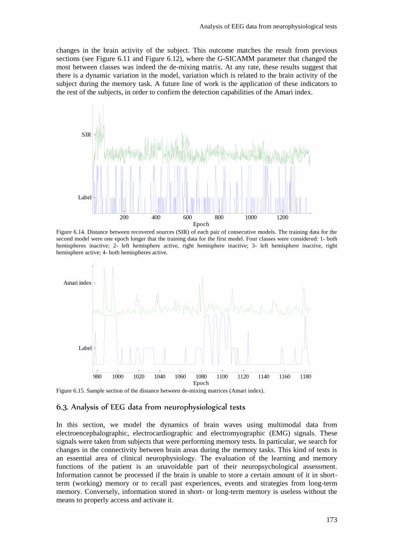
Analysis of EEG data from neurophysiological tests
173
changes in the brain activity of the subject. This outcome matches the result from previous
sections (see Figure 6.11 and Figure 6.12), where the G-SICAMM parameter that changed the
most between classes was indeed the de-mixing matrix. At any rate, these results suggest that
there is a dynamic variation in the model, variation which is related to the brain activity of the
subject during the memory task. A future line of work is the application of these indicators to
the rest of the subjects, in order to confirm the detection capabilities of the Amari index.
Figure 6.14. Distance between recovered sources (SIR) of each pair of consecutive models. The training data for the
second model were one epoch longer that the training data for the first model. Four classes were considered: 1- both
hemispheres inactive; 2- left hemisphere active, right hemisphere inactive; 3- left hemisphere inactive, right
hemisphere active; 4- both hemispheres active.
Figure 6.15. Sample section of the distance between de-mixing matrices (Amari index).
6.3. Analysis of EEG data from neurophysiological tests
In this section, we model the dynamics of brain waves using multimodal data from
electroencephalographic, electrocardiographic and electromyographic (EMG) signals. These
signals were taken from subjects that were performing memory tests. In particular, we search for
changes in the connectivity between brain areas during the memory tasks. This kind of tests is
an essential area of clinical neurophysiology. The evaluation of the learning and memory
functions of the patient is an unavoidable part of their neuropsychological assessment.
Information cannot be processed if the brain is unable to store a certain amount of it in short-
term (working) memory or to recall past experiences, events and strategies from long-term
memory. Conversely, information stored in short- or long-term memory is useless without the
means to properly access and activate it.
200 400 600 800 1000 1200
Label
SIR
Epoch
980 1000 1020 1040 1060 1080 1100 1120 1140 1160 1180
Label
Amari index
Epoch
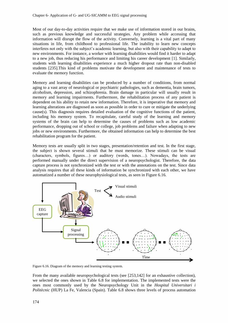
Chapter 6- Application of G- and UG-SICAMM to EEG signal processing
174
Most of our day-to-day activities require that we make use of information stored in our brains,
such as previous knowledge and successful strategies. Any problem while accessing that
information will disrupt the flow of the activity. Conversely, learning is a vital part of many
situations in life, from childhood to professional life. The inability to learn new concepts
interferes not only with the subject’s academic learning, but also with their capability to adapt to
new environments. For instance, a worker with learning disabilities would find it harder to adapt
to a new job, thus reducing his performance and limiting his career development [1]. Similarly,
students with learning disabilities experience a much higher dropout rate than non-disabled
students [235].This kind of problems motivate the development and maintenance of tests to
evaluate the memory function.
Memory and learning disabilities can be produced by a number of conditions, from normal
aging to a vast array of neurological or psychiatric pathologies, such as dementia, brain tumors,
alcoholism, depression, and schizophrenia. Brain damage in particular will usually result in
memory and learning impairments. Furthermore, the rehabilitation process of any patient is
dependent on his ability to retain new information. Therefore, it is imperative that memory and
learning alterations are diagnosed as soon as possible in order to cure or mitigate the underlying
cause(s). This diagnosis requires detailed evaluation of the cognitive functions of the patient,
including his memory system. To recapitulate, careful study of the learning and memory
systems of the brain can help to determine the causes of problems such as low academic
performance, dropping out of school or college, job problems and failure when adapting to new
jobs or new environments. Furthermore, the obtained information can help to determine the best
rehabilitation program for the patient.
Memory tests are usually split in two stages, presentation/retention and test. In the first stage,
the subject is shown several stimuli that he must memorize. These stimuli can be visual
(characters, symbols, figures…) or auditory (words, tones…). Nowadays, the tests are
performed manually under the direct supervision of a neuropsychologist. Therefore, the data
capture process is not synchronized with the test or with the annotations on the test. Since data
analysis requires that all these kinds of information be synchronized with each other, we have
automatized a number of these neurophysiological tests, as seen in Figure 6.16.
Figure 6.16. Diagram of the memory and learning testing system.
From the many available neuropsychological tests (see [253,142] for an exhaustive collection),
we selected the ones shown in Table 6.8 for implementation. The implemented tests were the
ones most commonly used by the Neuropsychology Unit in the Hospital Universitari i
Politècnic (HUP) La Fe, Valencia (Spain). Table 6.8 shows three levels of process automation
EEG capture
Test Visual stimuli
Audio stimuli
Signal
processing
Time

Analysis of EEG data from neurophysiological tests
175
for the tests: full, partial, and synch-only. Fully-automated tests are completely implemented on
the computer and require no work from the neuropsychologist. Partially-automated tests are also
automated, but they require some degree of collaboration on the part of the neuropsychologist.
Only-synchronized (“synch-only”) tests are not implemented on the computer, which is only
used to synchronize the test with the data and the annotations.
6.3.1. Neuropsychological tests
The implemented tests are explained in brief in this Section in order to make this chapter more
self-contained. The Sternberg test, also known as Sternberg memory task, was presented in
Section 5.4.2.
Most of the implemented tests include both the immediate and the delayed “conditions” or
paradigms. In the immediate condition, the stimulus is presented to the participant just before
the task. In the delayed condition, there is a longer delay (typically 20 minutes) after the stimuli
are presented and before the participant is told the task to perform. Typically, the immediate
condition is used to assess working or short-term memory, whereas the delayed condition is
more appropriate to evaluate long-term memory.
Name Stimuli Automation Studied brain
functions
Test de Aprendizaje Verbal España-
Complutense (TAVEC, [20])
Auditory Full Auditory memory
Wechsler Memory
Scale-R (WMS-R)
Visual Paired
Associates
Visual Full Visual memory
Figural
Memory
Visual Full Visual working
memory
Wechsler Memory
Scale III (WMS-
III)
Verbal
Paired
Associates
Auditory Full Auditory memory
Visual
Reproduction
Visual Full Visual memory
Mental
Control
Auditory Synch-only Executive
Wechsler Adult
Intelligence Scale
(WAIS-III)
Digit Span Auditory Full Auditory working
memory
Digit
Symbol-
Coding
Visual Full Processing speed
Symbol
Search
Visual Full Processing speed
Barcelona
Neuropsychological
Test (TB, [197])
Visual
Memory
Visual Full Visual working
memory
Stroop Color Word Visual Synch-only Executive
Trail Making Visual Full Attention
Boston Naming Visual Partial Language
Verbal Fluency Phonemic Auditory Synch-only Executive
Semantic Auditory Synch-only Executive
Sternberg [251] Visual Full Visual working
memory Table 6.8. Implemented neuropsychological tests. Tests were taken from [253] unless otherwise noted.

Chapter 6- Application of G- and UG-SICAMM to EEG signal processing
176
6.3.1.a. Test de Aprendizaje Verbal España-Complutense (TAVEC)
The Test de Aprendizaje Verbal España-Complutense (TAVEC, [20]) is a neuropsychological
test of auditory working memory and long-term memory. Based on the Rey Fifteen-Item Test
(FIT, [142]), the TAVEC introduces knowledge about neurocognitive models of the memory
function to interpret the results of the test [20]. This interpretation surpasses the “multi-storage”
model and integrates into modularity-of-mind theories. The TAVEC allows determining the
“normality” of a patient when compared against a similar normed sample and determining the
possible causes of any deviation. It is used for differential diagnosis of memory alterations such
as dementia, cognitive loss, traumatic brain injuries (TBI), and epilepsy.
The TAVEC comprises three different lists, Learning (list A), Interference (list B), and Recall.
In this work, only the Learning and Interference lists were implemented. Lists A and B are
composed of 16 words from four semantic categories, two in common for both lists (“spices”
and “fruit”) and two exclusive to each list: “tools” and “clothing” for list A; “fish” and “kitchen
utensils” for list B. In the immediate condition, the Learning list is read and the participant is
asked to repeat as many words as possible in any order. This process is repeated 5 times. The
Interference list is then read and the participant is required to repeat as many words as possible
from it. Finally, the participant is asked to recall the words from list A without listening to it. In
the delayed condition, the participant is asked to repeat as many words as possible from list A.
Scoring is calculated depending on the number of recalled items and the number of errors.
6.3.1.b. Wechsler Memory Scale
The Wechsler Memory Scale (WMS, [253]) is a neuropsychological test developed to detect
and evaluate memory disorders in adults and older adolescents. The original WMS was
published by Dr. David Wechsler in 1945, and it has been revised several times through the
years. The first revision, WMS-R, includes nine sub-tests and five indices that measured
different types of memory: Verbal Memory, Visual Memory, Delayed Recall,
Attention/Concentration, and General Memory. The next revision, WMS-III, added sub-tests to
assess delayed recognition memory and replaced abstract visual designs with pictures of
everyday stimuli (e.g., the Faces sub-test). The test includes eleven sub-tests, from which eight
primary index scores are derived. The WSM can be used to assess the clinically relevant aspects
of memory functioning. For example, it can be used to detect and localize cerebral dysfunction
and it can aid in detecting dementias and neurodegenerative disorders. Research suggests that
the primary indices of the WMS-III can accurately identify malingering of neurocognitive
dysfunction in mild TBI.
As shown in Table 6.8, five sub-tests were implemented: Visual Paired Associates and Figural
Memory (from WMS-R), and Verbal Paired Associates, Visual Reproduction and Mental
Control (from WMS-III).
The Visual Paired Associated sub-test evaluates visual memory and cued recall. It includes six
pairs of an abstract figure and a color. In the immediate condition, the participant is shown the
six pairs in succession. Afterward, the figures are shown one by one and the participant is told
to provide the corresponding color for each figure. There are three trials of the same pairs in
different orders. In the delayed condition, the examinee is shown the same figures and is asked
to choose the corresponding colors. Scoring is calculated from the number of correct pairs.
The Figural Memory sub-test is an immediate recognition test of abstract designs. The
participant is shown a set of three abstract figures, rectangles with a pattern of shapes inside
them, for 10 seconds. Afterward, the examinee is shown a set of nine similar figures from which
they have to select the three figures they were shown before. There are three trials of increasing
difficulty. Scoring is calculated from the number of correctly-selected figures.

Analysis of EEG data from neurophysiological tests
177
The Verbal Paired Associates sub-test evaluates auditory memory and cued recall. It is
composed of 10 to 14 word pairs; half of these pairs are semantically related (e.g., rose-flower)
and the other half are unrelated (e.g., cauliflower-pencil). In the immediate condition, after the
word pairs are read, the first word of each pair is read and the participant is told to provide the
corresponding word. There are three to six trials of the same list in different orders. In the
delayed condition, the examinee is orally presented with the first word of each pair learned in
the immediate condition and asked to provide the corresponding word. Scoring is calculated
from the number of correct pairs.
The Visual Reproduction sub-test assesses memory for non-verbal (i.e., abstract) visual stimuli.
In the immediate condition, the participant is shown a series of five designs for 10 seconds each.
After each design is presented, the participant is asked to draw the design from memory. In the
delayed condition, the examinee is asked to draw the designs shown during the immediate
condition from memory in any order. The result of the sub-test is calculated by a methodical
comparison of the copied figures and the original ones.
In the Mental Control sub-test, the participant is asked to perform seven verbal tasks of
increasing difficulty: i) counting from 1 to 20; ii) reciting the alphabet; iii) listing the days of the
week; iv) saying the months of the year; v) counting down from 20 to 1; vi) saying the days of
the week in reverse order; vi) saying the months of the year in reverse order; vii) counting from
0 to 36 by sixes and reciting the days of the week in alternating order (0-Monday, 6-Tuesday,
and so on until 36-Sunday). Scoring is calculated from the number of mistakes and the time
taken to complete each task.
6.3.1.c. Wechsler Adult Intelligence Scale
The Wechsler Adult Intelligence Scale (WAIS, [253]) is a test designed to measure intelligence
in adults and older adolescents. The first edition of the test was created in 1939, and it was
named the Wechsler-Bellevue intelligence scale (WB); later editions changed the name of the
test. It was developed by Dr. David Wechsler to replace the then-dominant Stanford-Binet scale
of intelligence. The third edition of the test (WAIS-III), unlike previous editions, measures
intelligence based on four factorially-derived indices. These indices enhance its clinical
relevance for differential diagnosis of conditions that are linked with intelligence, such as brain
injuries or learning disabilities. In neuropsychological assessment, the WAIS-III can: a)
diagnose cognitive disorders and identify brain dysfunction; b) track changes in cognitive
function over time; c) identify cognitive strengths and weaknesses important for daily
functioning. The test comprises seven verbal sub-tests and six non-verbal (performance) sub-
tests. Out of these, one verbal sub-test and two performance sub-tests were implemented, as
shown in Table 6.8: Digit Span, Digit Symbol-Coding, and Symbol Search.
The Digit Span sub-test is split in two stages. In the first one, called Digit Span Forward, the
participant is read a sequence of numbers and then recalls the numbers in the same order.
During the second stage, Digit Span Backward, the participant is read a sequence of numbers
and recalls the numbers in reverse order. In both stages, the objective is recalling correctly as
many sequences as possible.
In the Digit Symbol-Coding sub-test, the numbers 1 to 9 are paired with symbols on a key. The
participant is given the key and asked to go through a grid numbers and select the correct
symbols for each number. The sub-test is timed and scoring is given depending on the amount
of correct responses and the number of mistakes.
In the Symbol Search sub-test, the participant indicates whether one of the symbols in the target
group matches any of the symbols in the search group. This process is repeated as many times
as possible within a specified time limit, and scoring is given depending on the amount of
correct responses.

Chapter 6- Application of G- and UG-SICAMM to EEG signal processing
178
6.3.1.d. Barcelona Neuropsychological Test
The Barcelona Neuropsychological Test (TB, [197]) or Programa Integrado de Exploración
Neuropsicológica (PIEN) is a battery of tests designed in Spain in 1977 to evaluate higher
mental functions in such a way as to advance clinical knowledge of neuropsychological
patients. It is one of the first neuropsychological tests developed in Spain. It is a comprehensive
test that considers a high number of mental functions, such as: attention, language, orientation,
visual memory, and abstraction capability. It comprises 106 subtests split in 42 categories, and
the whole TB takes about 3 hours to complete. Successive revisions of the TB have reduced the
run time and complexity of the test, such as the abbreviated Barcelona test (TB-A, [198]). Only
the Visual Memory sub-test of the TB was implemented, as shown in Table 6.8.
In the Visual Memory sub-test, the participant is shown an abstract line figure during 10
seconds. Afterward, the participant is told to select the shown figure out of a group of four
similar figures. There are ten series in this sub-test, and scoring is given depending on the
number of correct responses.
6.3.1.e. Stroop Color Word Test
The Stroop Color Word Test (SCWT, [253]) is based on the Stroop effect, discovered in 1935
by its namesake, Dr. John Ridley Stroop. In brief, the Stroop effect consists in that we are able
to read words more quickly and automatically than we can name colors. For instance, if one is
presented with the word “blue” printed in red ink, he will say the word “blue” more readily than
he can name the color in which it is printed, red. The SCWT uses this effect to assess the ability
of an individual to inhibit a habitual response for one that is less readily available. It provides
insight into cognitive effects that are experienced as a result of attentional fatigue. Also,
performance in the SCWT is lower in patients with dementia and in individuals with frontal
lobe versus posterior lesions and left versus right hemisphere lesions.
The SCWT is composed of three stages, Color, Word, and Color-Word. In the first stage, Color,
the participant is given a sheet of paper with a 5x20 grid of bars that are colored red, green or
blue. Participants are instructed to say the color of each bar going down the columns. In the
Word stage, the bars are replaced with color words (red, green, blue) in black type, and the
participant is required to read the words. Finally, in the Color-Word stage, each word is printed
in a color that differs from the written word (e.g., the word “red” will be printed in blue or
green, not in red). The participant is instructed to say the color of the item, not the written word.
Participants are given 45 seconds for each stage, with scoring being given by the number of
correct responses.
6.3.1.f. Trail Making Test
The Trail Making Test (TMT, [253]) is a neuropsychological test of attention, processing speed,
and task switching. It was developed in 1938 by US Army psychologists, and adapted to civil
use in 1955. The TMT is one of the best measures of attention and one of the most popular
neuropsychological tests. The test is highly sensitive to brain injury, and it can be used for
differential diagnosis of several conditions, such as alcoholism and learning disabilities.
The TMT has two parts, A and B. In part A, participants are instructed to connect 25 encircled
numbers that have been randomly placed on a page. The numbers have to be connected in
proper order within 5 minutes, without making mistakes or lifting the pencil from the paper. In
part B, the participants are required to connect 25 encircled numbers and letters in alternating
order, again within 5 minutes. In both parts, participants are instructed to connect the circles as
fast as they can. The test is scored based on the time taken to complete each part. The number of
errors may be clinically relevant, but it is not a separate score.
Analysis of EEG data from neurophysiological tests
179
6.3.1.g. Boston Naming Test
The Boston Naming Test (BNT, [253]) is a visual confrontation naming test used to measure
confrontational word retrieval in individuals. This ability is diminished in patients with strokes,
Alzheimer’s disease, and other dementing disorders. However, there is limited normative data,
and the BNT is usually used as a supplement to other neuropsychological tests.
The BNT contains 60 line drawings graded in ascending difficulty, that is, frequency of use.
The drawings are shown one at a time and the participant is asked to name each of them within
20 seconds. The examinee may be presented with cues when there is a mistaken response; these
cues can be descriptive or phonemic. The total score is the number of accurate responses,
disregarding those following a phonemic cue.
6.3.1.h. Verbal Fluency
Verbal fluency is a cognitive function that facilitates information retrieval from memory. There
are a number of verbal fluency tests that date back to the 1960’s. The two most commonly-
measured parameters are ( [142]): a) semantic fluency, tested by asking the participant to
generate as many words from a given category as possible (animals, clothing…); b) phonemic
fluency, which is tested by asking the participant to generate words beginning with a single
letter (f, a, s…). Neuroimaging studies suggest that the two types of fluency tasks may engage
different cognitive processes and are differentially affected in clinical populations. Results show
a number of consistent characteristics across types and subjects, such as the production of bursts
of semantically-related words and a hyperbolic decline in the rate of production of new words.
In this work, three verbal fluency tasks were considered: two phonemic fluency tasks (word
beginning with “f” and with “a”) and one semantic fluency task (animals). In all cases, the
participant was asked to provide as many words as possible within 60 seconds.
6.3.2. Experiment configuration
The experiment was performed on six epileptic patients, between 32 and 67 years old. Each
patient was fitted with several electrodes with which to record the EEG, ECG and EMG signals
for the duration of the neuropsychological testing. The location of the EEG electrodes is shown
in Figure 6.17; note that they are different from the locations of the electrodes in Figure 5.19.
Two ECG electrodes were placed in a modification of Lead II of the American Heart
Association. One of the electrodes was placed on the right hemithorax and the other on the left
inframammary region, close to the sixth intercostal space. This lead was selected because we
were more interested in the sequence of the EEG, rather than in its fine detail.
The recorded signals were composed by 18 bipolar EEG channels and one bipolar
electrocardiographic channel. The data were captured with a sampling frequency of 512 Hz, and
then band-pass filtered between 1.6 and 35 Hz using clinical-purpose software. The data
recording and filtering process was performed by specialists of the Neurology Unit of the La Fe
hospital. The signals and the test results were registered by different devices, and special care
was taken to ensure the correct synchronization between the capture devices and the computer
performing the tests. A neuropsychologist was present at all times to guide and supervise the
participant during the test taking process.
The implementation of each test was different depending on whether the test requires visual or
auditory stimuli, as indicated in Table 6.8. The visual tests were built as graphical user
interfaces using MATLAB®, a high-level language and interactive environment for numerical
computation. Each GUI is composed of a graphical front end and a numerical back end. The
front end for the WAIS-III Symbol Search sub-test is shown in Figure 6.18; the rest of the front
ends look very similar to it. The tests were presented on a large touchscreen in order to simplify
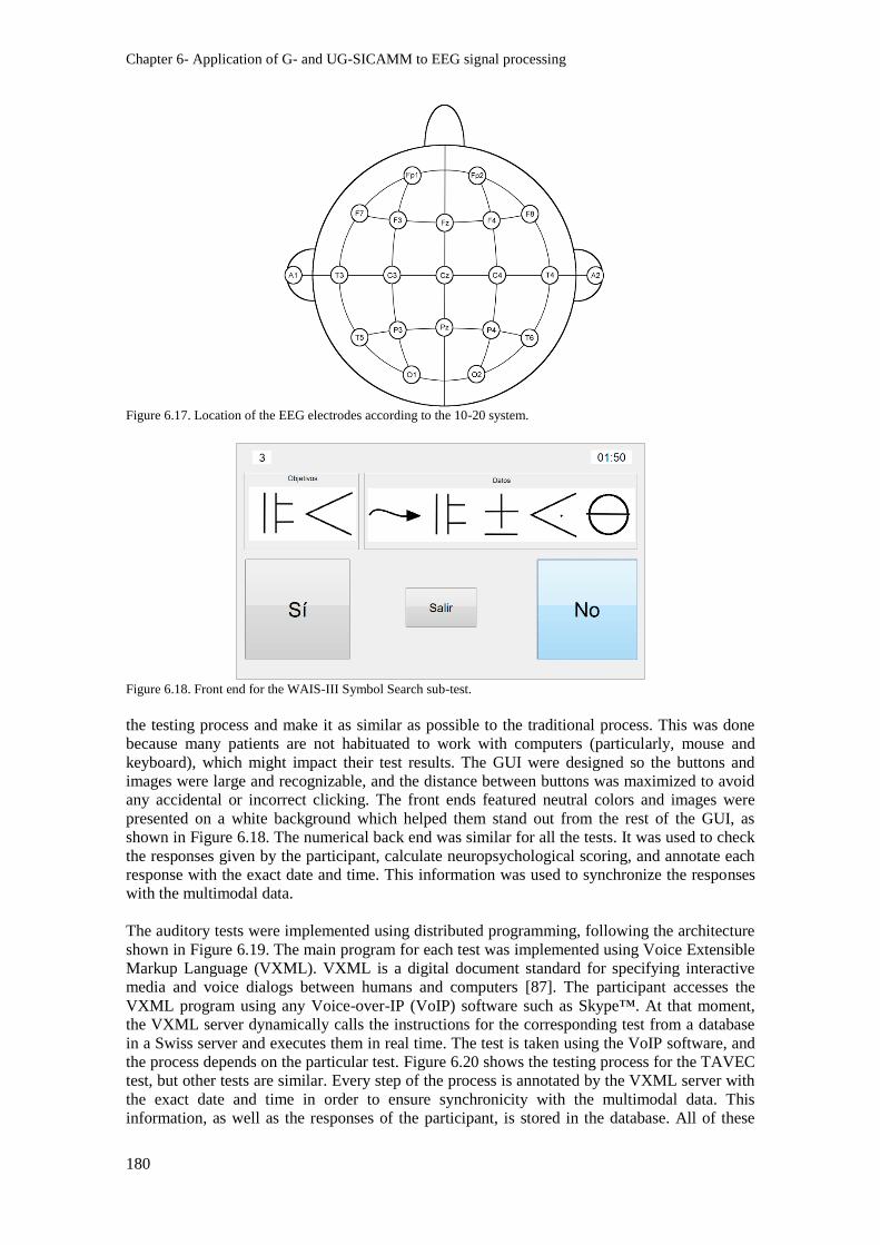
Chapter 6- Application of G- and UG-SICAMM to EEG signal processing
180
Figure 6.17. Location of the EEG electrodes according to the 10-20 system.
Figure 6.18. Front end for the WAIS-III Symbol Search sub-test.
the testing process and make it as similar as possible to the traditional process. This was done
because many patients are not habituated to work with computers (particularly, mouse and
keyboard), which might impact their test results. The GUI were designed so the buttons and
images were large and recognizable, and the distance between buttons was maximized to avoid
any accidental or incorrect clicking. The front ends featured neutral colors and images were
presented on a white background which helped them stand out from the rest of the GUI, as
shown in Figure 6.18. The numerical back end was similar for all the tests. It was used to check
the responses given by the participant, calculate neuropsychological scoring, and annotate each
response with the exact date and time. This information was used to synchronize the responses
with the multimodal data.
The auditory tests were implemented using distributed programming, following the architecture
shown in Figure 6.19. The main program for each test was implemented using Voice Extensible
Markup Language (VXML). VXML is a digital document standard for specifying interactive
media and voice dialogs between humans and computers [87]. The participant accesses the
VXML program using any Voice-over-IP (VoIP) software such as Skype™. At that moment,
the VXML server dynamically calls the instructions for the corresponding test from a database
in a Swiss server and executes them in real time. The test is taken using the VoIP software, and
the process depends on the particular test. Figure 6.20 shows the testing process for the TAVEC
test, but other tests are similar. Every step of the process is annotated by the VXML server with
the exact date and time in order to ensure synchronicity with the multimodal data. This
information, as well as the responses of the participant, is stored in the database. All of these
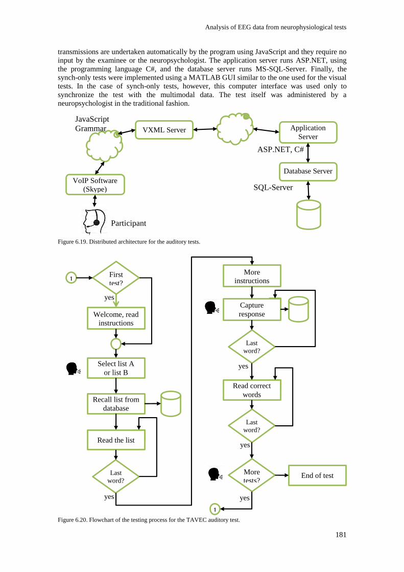
Analysis of EEG data from neurophysiological tests
181
transmissions are undertaken automatically by the program using JavaScript and they require no
input by the examinee or the neuropsychologist. The application server runs ASP.NET, using
the programming language C#, and the database server runs MS-SQL-Server. Finally, the
synch-only tests were implemented using a MATLAB GUI similar to the one used for the visual
tests. In the case of synch-only tests, however, this computer interface was used only to
synchronize the test with the multimodal data. The test itself was administered by a
neuropsychologist in the traditional fashion.
Figure 6.19. Distributed architecture for the auditory tests.
Figure 6.20. Flowchart of the testing process for the TAVEC auditory test.
VXML Server
VoIP Software
(Skype)
Application
Server
Database Server
Participant
JavaScript
Grammar
ASP.NET, C#
SQL-Server
1 First
test?
Welcome, read
instructions
Select list A
or list B
Recall list from
database
Read the list
Last
word?
More
instructions
Capture
response
Last
word?
Read correct
words
Last
word?
More
tests? End of test
1
yes
yes
yes
yes
yes
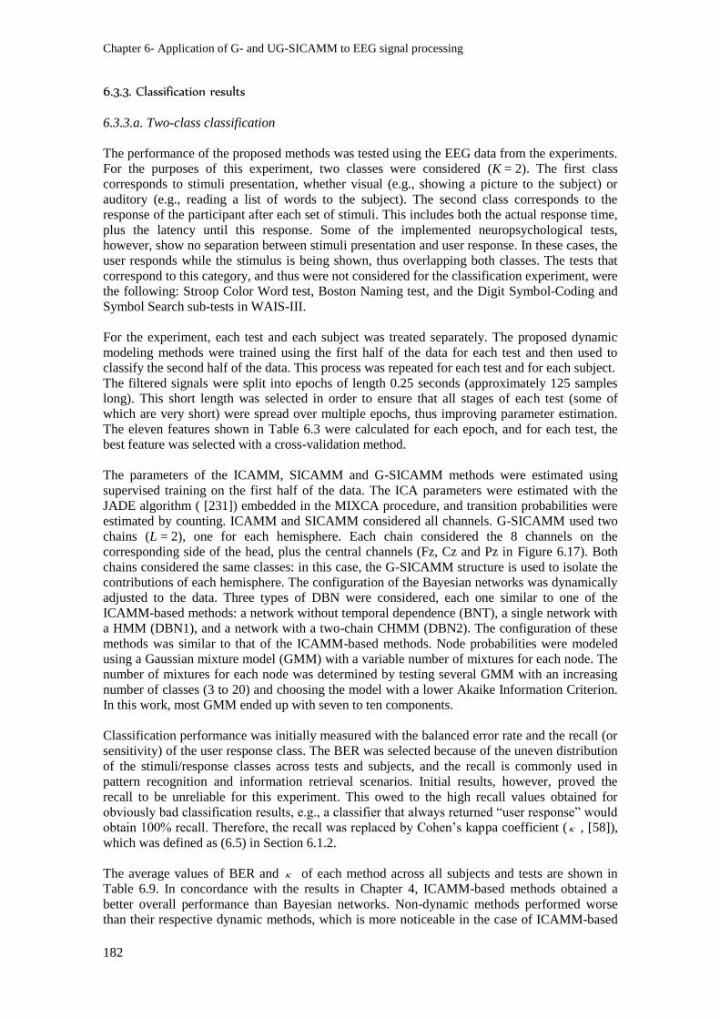
Chapter 6- Application of G- and UG-SICAMM to EEG signal processing
182
6.3.3. Classification results
6.3.3.a. Two-class classification
The performance of the proposed methods was tested using the EEG data from the experiments.
For the purposes of this experiment, two classes were considered (K = 2). The first class
corresponds to stimuli presentation, whether visual (e.g., showing a picture to the subject) or
auditory (e.g., reading a list of words to the subject). The second class corresponds to the
response of the participant after each set of stimuli. This includes both the actual response time,
plus the latency until this response. Some of the implemented neuropsychological tests,
however, show no separation between stimuli presentation and user response. In these cases, the
user responds while the stimulus is being shown, thus overlapping both classes. The tests that
correspond to this category, and thus were not considered for the classification experiment, were
the following: Stroop Color Word test, Boston Naming test, and the Digit Symbol-Coding and
Symbol Search sub-tests in WAIS-III.
For the experiment, each test and each subject was treated separately. The proposed dynamic
modeling methods were trained using the first half of the data for each test and then used to
classify the second half of the data. This process was repeated for each test and for each subject.
The filtered signals were split into epochs of length 0.25 seconds (approximately 125 samples
long). This short length was selected in order to ensure that all stages of each test (some of
which are very short) were spread over multiple epochs, thus improving parameter estimation.
The eleven features shown in Table 6.3 were calculated for each epoch, and for each test, the
best feature was selected with a cross-validation method.
The parameters of the ICAMM, SICAMM and G-SICAMM methods were estimated using
supervised training on the first half of the data. The ICA parameters were estimated with the
JADE algorithm ( [231]) embedded in the MIXCA procedure, and transition probabilities were
estimated by counting. ICAMM and SICAMM considered all channels. G-SICAMM used two
chains (L = 2), one for each hemisphere. Each chain considered the 8 channels on the
corresponding side of the head, plus the central channels (Fz, Cz and Pz in Figure 6.17). Both
chains considered the same classes: in this case, the G-SICAMM structure is used to isolate the
contributions of each hemisphere. The configuration of the Bayesian networks was dynamically
adjusted to the data. Three types of DBN were considered, each one similar to one of the
ICAMM-based methods: a network without temporal dependence (BNT), a single network with
a HMM (DBN1), and a network with a two-chain CHMM (DBN2). The configuration of these
methods was similar to that of the ICAMM-based methods. Node probabilities were modeled
using a Gaussian mixture model (GMM) with a variable number of mixtures for each node. The
number of mixtures for each node was determined by testing several GMM with an increasing
number of classes (3 to 20) and choosing the model with a lower Akaike Information Criterion.
In this work, most GMM ended up with seven to ten components.
Classification performance was initially measured with the balanced error rate and the recall (or
sensitivity) of the user response class. The BER was selected because of the uneven distribution
of the stimuli/response classes across tests and subjects, and the recall is commonly used in
pattern recognition and information retrieval scenarios. Initial results, however, proved the
recall to be unreliable for this experiment. This owed to the high recall values obtained for
obviously bad classification results, e.g., a classifier that always returned “user response” would
obtain 100% recall. Therefore, the recall was replaced by Cohen’s kappa coefficient ( , [58]),
which was defined as (6.5) in Section 6.1.2.
The average values of BER and of each method across all subjects and tests are shown in
Table 6.9. In concordance with the results in Chapter 4, ICAMM-based methods obtained a
better overall performance than Bayesian networks. Non-dynamic methods performed worse
than their respective dynamic methods, which is more noticeable in the case of ICAMM-based
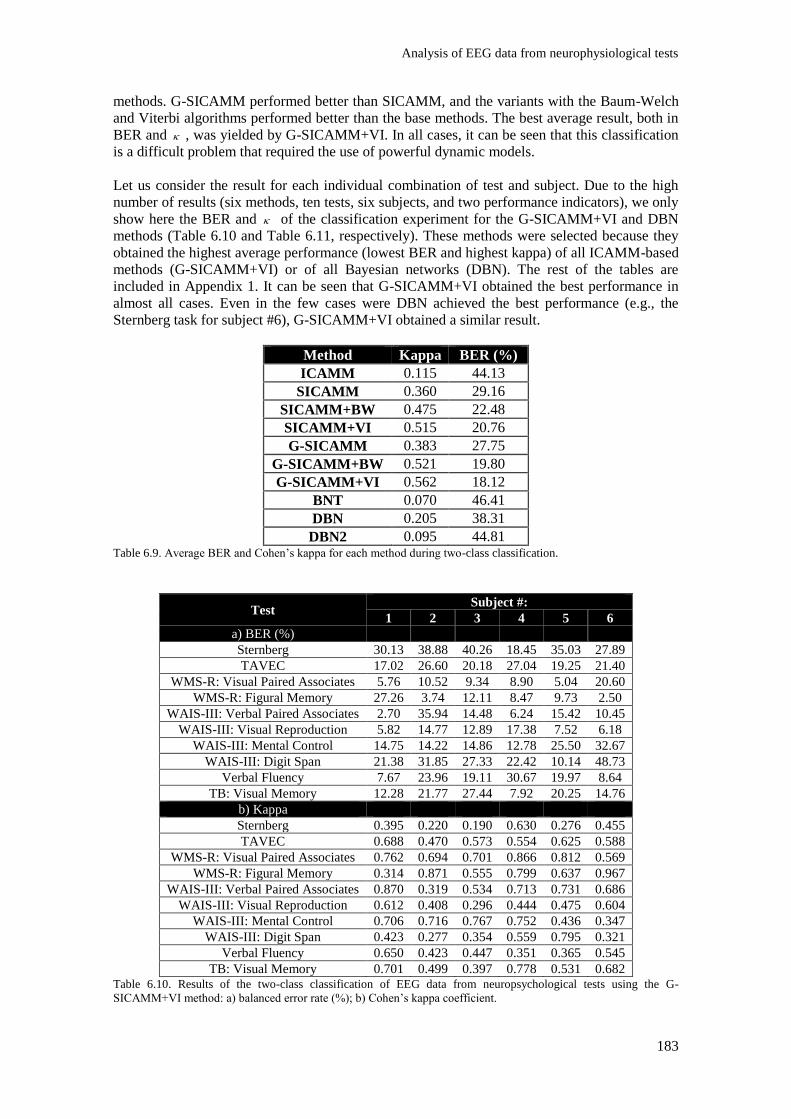
Analysis of EEG data from neurophysiological tests
183
methods. G-SICAMM performed better than SICAMM, and the variants with the Baum-Welch
and Viterbi algorithms performed better than the base methods. The best average result, both in
BER and , was yielded by G-SICAMM+VI. In all cases, it can be seen that this classification
is a difficult problem that required the use of powerful dynamic models.
Let us consider the result for each individual combination of test and subject. Due to the high
number of results (six methods, ten tests, six subjects, and two performance indicators), we only
show here the BER and of the classification experiment for the G-SICAMM+VI and DBN
methods (Table 6.10 and Table 6.11, respectively). These methods were selected because they
obtained the highest average performance (lowest BER and highest kappa) of all ICAMM-based
methods (G-SICAMM+VI) or of all Bayesian networks (DBN). The rest of the tables are
included in Appendix 1. It can be seen that G-SICAMM+VI obtained the best performance in
almost all cases. Even in the few cases were DBN achieved the best performance (e.g., the
Sternberg task for subject #6), G-SICAMM+VI obtained a similar result.
Method Kappa BER (%)
ICAMM 0.115 44.13
SICAMM 0.360 29.16
SICAMM+BW 0.475 22.48
SICAMM+VI 0.515 20.76
G-SICAMM 0.383 27.75
G-SICAMM+BW 0.521 19.80
G-SICAMM+VI 0.562 18.12
BNT 0.070 46.41
DBN 0.205 38.31
DBN2 0.095 44.81 Table 6.9. Average BER and Cohen’s kappa for each method during two-class classification.
Test Subject #:
1 2 3 4 5 6
a) BER (%)
Sternberg 30.13 38.88 40.26 18.45 35.03 27.89
TAVEC 17.02 26.60 20.18 27.04 19.25 21.40
WMS-R: Visual Paired Associates 5.76 10.52 9.34 8.90 5.04 20.60
WMS-R: Figural Memory 27.26 3.74 12.11 8.47 9.73 2.50
WAIS-III: Verbal Paired Associates 2.70 35.94 14.48 6.24 15.42 10.45
WAIS-III: Visual Reproduction 5.82 14.77 12.89 17.38 7.52 6.18
WAIS-III: Mental Control 14.75 14.22 14.86 12.78 25.50 32.67
WAIS-III: Digit Span 21.38 31.85 27.33 22.42 10.14 48.73
Verbal Fluency 7.67 23.96 19.11 30.67 19.97 8.64
TB: Visual Memory 12.28 21.77 27.44 7.92 20.25 14.76
b) Kappa
Sternberg 0.395 0.220 0.190 0.630 0.276 0.455
TAVEC 0.688 0.470 0.573 0.554 0.625 0.588
WMS-R: Visual Paired Associates 0.762 0.694 0.701 0.866 0.812 0.569
WMS-R: Figural Memory 0.314 0.871 0.555 0.799 0.637 0.967
WAIS-III: Verbal Paired Associates 0.870 0.319 0.534 0.713 0.731 0.686
WAIS-III: Visual Reproduction 0.612 0.408 0.296 0.444 0.475 0.604
WAIS-III: Mental Control 0.706 0.716 0.767 0.752 0.436 0.347
WAIS-III: Digit Span 0.423 0.277 0.354 0.559 0.795 0.321
Verbal Fluency 0.650 0.423 0.447 0.351 0.365 0.545
TB: Visual Memory 0.701 0.499 0.397 0.778 0.531 0.682 Table 6.10. Results of the two-class classification of EEG data from neuropsychological tests using the G-
SICAMM+VI method: a) balanced error rate (%); b) Cohen’s kappa coefficient.
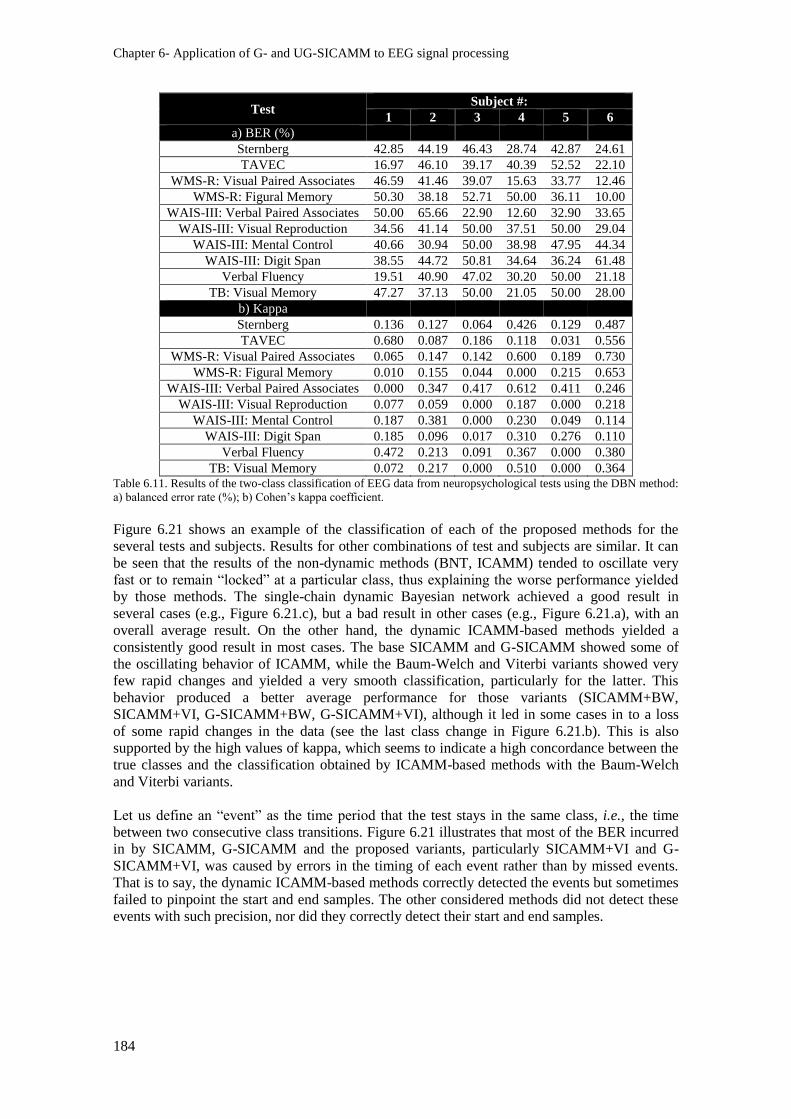
Chapter 6- Application of G- and UG-SICAMM to EEG signal processing
184
Test Subject #:
1 2 3 4 5 6
a) BER (%)
Sternberg 42.85 44.19 46.43 28.74 42.87 24.61
TAVEC 16.97 46.10 39.17 40.39 52.52 22.10
WMS-R: Visual Paired Associates 46.59 41.46 39.07 15.63 33.77 12.46
WMS-R: Figural Memory 50.30 38.18 52.71 50.00 36.11 10.00
WAIS-III: Verbal Paired Associates 50.00 65.66 22.90 12.60 32.90 33.65
WAIS-III: Visual Reproduction 34.56 41.14 50.00 37.51 50.00 29.04
WAIS-III: Mental Control 40.66 30.94 50.00 38.98 47.95 44.34
WAIS-III: Digit Span 38.55 44.72 50.81 34.64 36.24 61.48
Verbal Fluency 19.51 40.90 47.02 30.20 50.00 21.18
TB: Visual Memory 47.27 37.13 50.00 21.05 50.00 28.00
b) Kappa
Sternberg 0.136 0.127 0.064 0.426 0.129 0.487
TAVEC 0.680 0.087 0.186 0.118 0.031 0.556
WMS-R: Visual Paired Associates 0.065 0.147 0.142 0.600 0.189 0.730
WMS-R: Figural Memory 0.010 0.155 0.044 0.000 0.215 0.653
WAIS-III: Verbal Paired Associates 0.000 0.347 0.417 0.612 0.411 0.246
WAIS-III: Visual Reproduction 0.077 0.059 0.000 0.187 0.000 0.218
WAIS-III: Mental Control 0.187 0.381 0.000 0.230 0.049 0.114
WAIS-III: Digit Span 0.185 0.096 0.017 0.310 0.276 0.110
Verbal Fluency 0.472 0.213 0.091 0.367 0.000 0.380
TB: Visual Memory 0.072 0.217 0.000 0.510 0.000 0.364 Table 6.11. Results of the two-class classification of EEG data from neuropsychological tests using the DBN method:
a) balanced error rate (%); b) Cohen’s kappa coefficient.
Figure 6.21 shows an example of the classification of each of the proposed methods for the
several tests and subjects. Results for other combinations of test and subjects are similar. It can
be seen that the results of the non-dynamic methods (BNT, ICAMM) tended to oscillate very
fast or to remain “locked” at a particular class, thus explaining the worse performance yielded
by those methods. The single-chain dynamic Bayesian network achieved a good result in
several cases (e.g., Figure 6.21.c), but a bad result in other cases (e.g., Figure 6.21.a), with an
overall average result. On the other hand, the dynamic ICAMM-based methods yielded a
consistently good result in most cases. The base SICAMM and G-SICAMM showed some of
the oscillating behavior of ICAMM, while the Baum-Welch and Viterbi variants showed very
few rapid changes and yielded a very smooth classification, particularly for the latter. This
behavior produced a better average performance for those variants (SICAMM+BW,
SICAMM+VI, G-SICAMM+BW, G-SICAMM+VI), although it led in some cases in to a loss
of some rapid changes in the data (see the last class change in Figure 6.21.b). This is also
supported by the high values of kappa, which seems to indicate a high concordance between the
true classes and the classification obtained by ICAMM-based methods with the Baum-Welch
and Viterbi variants.
Let us define an “event” as the time period that the test stays in the same class, i.e., the time
between two consecutive class transitions. Figure 6.21 illustrates that most of the BER incurred
in by SICAMM, G-SICAMM and the proposed variants, particularly SICAMM+VI and G-
SICAMM+VI, was caused by errors in the timing of each event rather than by missed events.
That is to say, the dynamic ICAMM-based methods correctly detected the events but sometimes
failed to pinpoint the start and end samples. The other considered methods did not detect these
events with such precision, nor did they correctly detect their start and end samples.
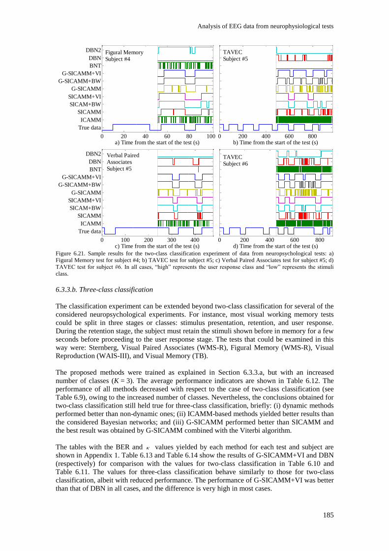
Analysis of EEG data from neurophysiological tests
185
Figure 6.21. Sample results for the two-class classification experiment of data from neuropsychological tests: a)
Figural Memory test for subject #4; b) TAVEC test for subject #5; c) Verbal Paired Associates test for subject #5; d)
TAVEC test for subject #6. In all cases, “high” represents the user response class and “low” represents the stimuli
class.
6.3.3.b. Three-class classification
The classification experiment can be extended beyond two-class classification for several of the
considered neuropsychological experiments. For instance, most visual working memory tests
could be split in three stages or classes: stimulus presentation, retention, and user response.
During the retention stage, the subject must retain the stimuli shown before in memory for a few
seconds before proceeding to the user response stage. The tests that could be examined in this
way were: Sternberg, Visual Paired Associates (WMS-R), Figural Memory (WMS-R), Visual
Reproduction (WAIS-III), and Visual Memory (TB).
The proposed methods were trained as explained in Section 6.3.3.a, but with an increased
number of classes (K = 3). The average performance indicators are shown in Table 6.12. The
performance of all methods decreased with respect to the case of two-class classification (see
Table 6.9), owing to the increased number of classes. Nevertheless, the conclusions obtained for
two-class classification still held true for three-class classification, briefly: (i) dynamic methods
performed better than non-dynamic ones; (ii) ICAMM-based methods yielded better results than
the considered Bayesian networks; and (iii) G-SICAMM performed better than SICAMM and
the best result was obtained by G-SICAMM combined with the Viterbi algorithm.
The tables with the BER and values yielded by each method for each test and subject are
shown in Appendix 1. Table 6.13 and Table 6.14 show the results of G-SICAMM+VI and DBN
(respectively) for comparison with the values for two-class classification in Table 6.10 and
Table 6.11. The values for three-class classification behave similarly to those for two-class
classification, albeit with reduced performance. The performance of G-SICAMM+VI was better
than that of DBN in all cases, and the difference is very high in most cases.
0 20 40 60 80 100
True data
ICAMM
SICAMM
SICAM+BW
SICAMM+VI
G-SICAMM
G-SICAMM+BW
G-SICAMM+VI
BNT
DBN
DBN2
a) Time from the start of the test (s)0 200 400 600 800
b) Time from the start of the test (s)
0 100 200 300 400
True data
ICAMM
SICAMM
SICAM+BW
SICAMM+VI
G-SICAMM
G-SICAMM+BW
G-SICAMM+VI
BNT
DBN
DBN2
c) Time from the start of the test (s)0 200 400 600 800
d) Time from the start of the test (s)
TAVECSubject #5
Figural MemorySubject #4
Verbal Paired AssociatesSubject #5
TAVECSubject #6
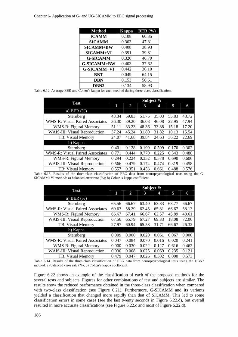
Chapter 6- Application of G- and UG-SICAMM to EEG signal processing
186
Method Kappa BER (%)
ICAMM 0.108 60.35
SICAMM 0.303 47.81
SICAMM+BW 0.408 38.93
SICAMM+VI 0.391 39.81
G-SICAMM 0.320 46.70
G-SICAMM+BW 0.403 37.62
G-SICAMM+VI 0.442 36.10
BNT 0.049 64.15
DBN 0.153 56.61
DBN2 0.134 58.93 Table 6.12. Average BER and Cohen’s kappa for each method during three-class classification.
Test Subject #:
1 2 3 4 5 6
a) BER (%)
Sternberg 43.34 59.83 51.75 35.03 55.83 48.72
WMS-R: Visual Paired Associates 36.30 39.20 36.08 46.08 22.95 47.94
WMS-R: Figural Memory 51.11 33.23 48.36 33.88 15.18 17.20
WAIS-III: Visual Reproduction 37.24 45.24 31.80 31.82 10.13 15.54
TB: Visual Memory 24.07 41.68 39.84 24.63 36.22 22.69
b) Kappa
Sternberg 0.401 0.128 0.199 0.509 0.170 0.302
WMS-R: Visual Paired Associates 0.771 0.444 0.770 0.225 0.543 0.488
WMS-R: Figural Memory 0.294 0.224 0.352 0.578 0.690 0.606
WAIS-III: Visual Reproduction 0.566 0.479 0.174 0.474 0.319 0.458
TB: Visual Memory 0.557 0.351 0.453 0.661 0.488 0.576 Table 6.13. Results of the three-class classification of EEG data from neuropsychological tests using the G-
SICAMM+VI method: a) balanced error rate (%); b) Cohen’s kappa coefficient.
Test Subject #:
1 2 3 4 5 6
a) BER (%)
Sternberg 65.56 66.67 63.40 63.83 63.77 66.67
WMS-R: Visual Paired Associates 69.63 58.29 62.45 65.81 66.67 58.13
WMS-R: Figural Memory 66.67 67.41 66.67 62.57 45.89 48.61
WAIS-III: Visual Reproduction 67.56 65.79 67.27 69.33 18.08 72.06
TB: Visual Memory 27.97 60.94 65.58 31.71 66.67 26.32
b) Kappa
Sternberg 0.009 0.000 0.020 0.061 0.067 0.000
WMS-R: Visual Paired Associates 0.047 0.084 0.070 0.016 0.020 0.241
WMS-R: Figural Memory 0.000 0.030 0.022 0.127 0.616 0.462
WAIS-III: Visual Reproduction 0.030 0.008 0.025 0.069 0.235 0.121
TB: Visual Memory 0.479 0.047 0.026 0.502 0.000 0.573 Table 6.14. Results of the three-class classification of EEG data from neuropsychological tests using the DBN2
method: a) balanced error rate (%); b) Cohen’s kappa coefficient.
Figure 6.22 shows an example of the classification of each of the proposed methods for the
several tests and subjects. Figures for other combinations of test and subjects are similar. The
results show the reduced performance obtained in the three-class classification when compared
with two-class classification (see Figure 6.21). Furthermore, G-SICAMM and its variants
yielded a classification that changed more rapidly than that of SICAMM. This led to some
classification errors in some cases (see the last twenty seconds in Figure 6.22.d), but overall
resulted in more accurate classifications (see Figure 6.22.c and most of Figure 6.22.d).
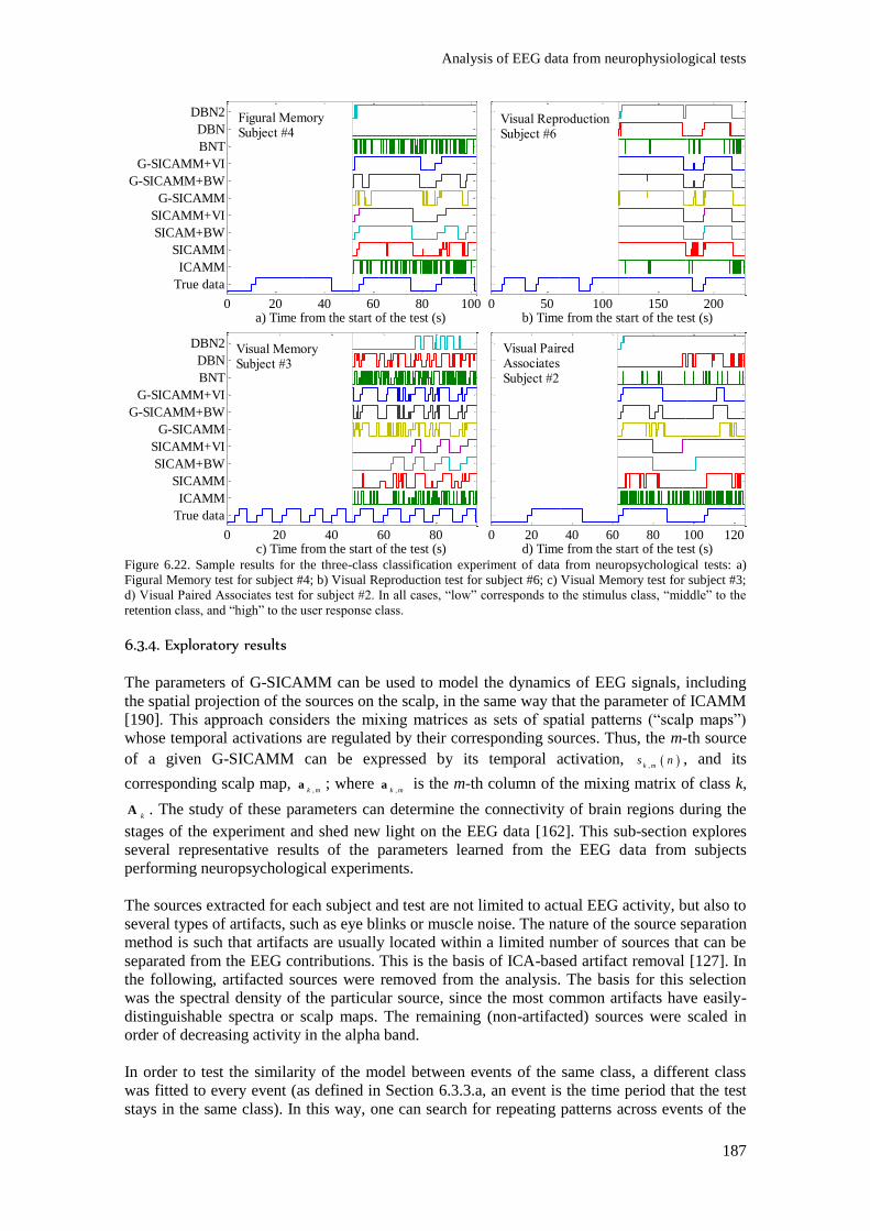
Analysis of EEG data from neurophysiological tests
187
Figure 6.22. Sample results for the three-class classification experiment of data from neuropsychological tests: a)
Figural Memory test for subject #4; b) Visual Reproduction test for subject #6; c) Visual Memory test for subject #3;
d) Visual Paired Associates test for subject #2. In all cases, “low” corresponds to the stimulus class, “middle” to the
retention class, and “high” to the user response class.
6.3.4. Exploratory results
The parameters of G-SICAMM can be used to model the dynamics of EEG signals, including
the spatial projection of the sources on the scalp, in the same way that the parameter of ICAMM
[190]. This approach considers the mixing matrices as sets of spatial patterns (“scalp maps”)
whose temporal activations are regulated by their corresponding sources. Thus, the m-th source
of a given G-SICAMM can be expressed by its temporal activation, ,k ms n , and its
corresponding scalp map, ,k m
a ; where ,k m
a is the m-th column of the mixing matrix of class k,
kA . The study of these parameters can determine the connectivity of brain regions during the
stages of the experiment and shed new light on the EEG data [162]. This sub-section explores
several representative results of the parameters learned from the EEG data from subjects
performing neuropsychological experiments.
The sources extracted for each subject and test are not limited to actual EEG activity, but also to
several types of artifacts, such as eye blinks or muscle noise. The nature of the source separation
method is such that artifacts are usually located within a limited number of sources that can be
separated from the EEG contributions. This is the basis of ICA-based artifact removal [127]. In
the following, artifacted sources were removed from the analysis. The basis for this selection
was the spectral density of the particular source, since the most common artifacts have easily-
distinguishable spectra or scalp maps. The remaining (non-artifacted) sources were scaled in
order of decreasing activity in the alpha band.
In order to test the similarity of the model between events of the same class, a different class
was fitted to every event (as defined in Section 6.3.3.a, an event is the time period that the test
stays in the same class). In this way, one can search for repeating patterns across events of the
0 20 40 60 80 100
True data
ICAMM
SICAMM
SICAM+BW
SICAMM+VI
G-SICAMM
G-SICAMM+BW
G-SICAMM+VI
BNT
DBN
DBN2
a) Time from the start of the test (s)0 50 100 150 200
b) Time from the start of the test (s)
0 20 40 60 80
True data
ICAMM
SICAMM
SICAM+BW
SICAMM+VI
G-SICAMM
G-SICAMM+BW
G-SICAMM+VI
BNT
DBN
DBN2
c) Time from the start of the test (s)0 20 40 60 80 100 120
d) Time from the start of the test (s)
Figural MemorySubject #4
Visual ReproductionSubject #6
Visual MemorySubject #3
Visual PairedAssociatesSubject #2
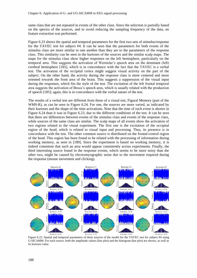
Chapter 6- Application of G- and UG-SICAMM to EEG signal processing
188
same class that are not repeated in events of the other class. Since the selection is partially based
on the spectra of the sources, and to avoid reducing the sampling frequency of the data, no
feature extraction was performed.
Figure 6.23 shows the spatial and temporal parameters for the first two sets of stimulus/response
for the TAVEC test for subject #4. It can be seen that the parameters for both events of the
stimulus class are more similar to one another than they are to the parameters of the response
class. This similarity can be seen in the kurtoses of the sources and the similar scalp maps. The
maps for the stimulus class show higher responses on the left hemisphere, particularly on the
temporal area. This suggests the activation of Wernicke’s speech area on the dominant (left)
cerebral hemisphere [185], which is in concordance with the fact that the TAVEC is a verbal
test. The activation of the occipital cortex might suggest visual activity on the part of the
subject. On the other hand, the activity during the response class is more centered and more
oriented towards the front area of the brain. This suggests a suppression of the visual input
during the responses, which fits the style of the test. The excitation of the left frontal temporal
area suggests the activation of Broca’s speech area, which is usually related with the production
of speech [185]; again, this is in concordance with the verbal nature of the test.
The results of a verbal test are different from those of a visual test, Figural Memory (part of the
WMS-R), as can be seen in Figure 6.24. For one, the sources are more varied, as indicated by
their kurtoses and the shape of the time activations. Note that the time of each event is shorter in
Figure 6.24 than it was in Figure 6.23, due to the different conditions of the test. It can be seen
that there are differences between events of the stimulus class and events of the response class,
while sources of the same class are similar. The scalp maps of all events show the activation of
two regions related to the visual experiment. The first one is the excitation of the occipital
region of the head, which is related to visual input and processing. Thus, its presence is in
concordance with the test. The other common source is distributed on the frontal-central region
of the head. This region has been found to be related with the processing of information during
working memory, as seen in [189]. Since the experiment is based on working memory, it is
indeed consistent that such an area would appear consistently across experiments. Finally, the
third interesting source found in the response events, which seems to be more noisy than the
other two, might be caused by electromyographic noise due to the movement required during
the response (mouse movement and clicking).
Figure 6.23. Spatial and temporal parameters of three sources of the model for the TAVEC test for subject #4 using
G-SICAMM. For each source, both the amplitude values (line plot) and the histogram (bar plot) are shown, as well as
its kurtosis value.
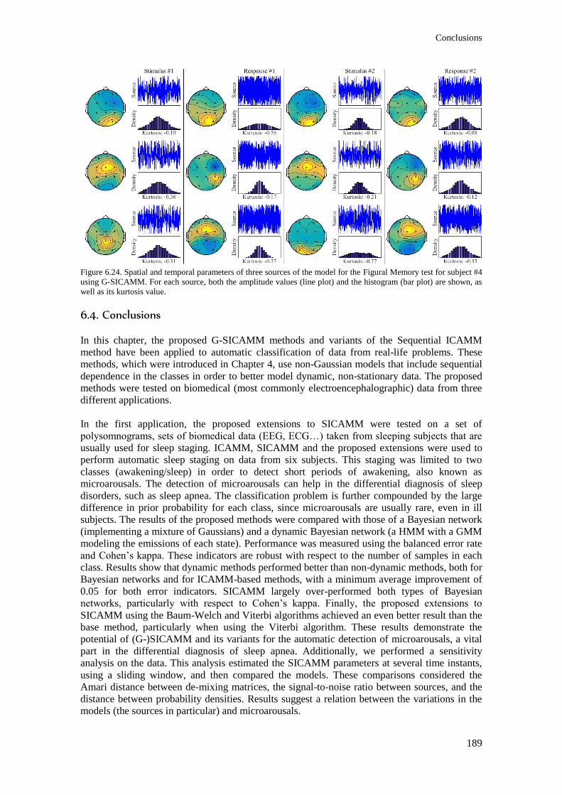
Conclusions
189
Figure 6.24. Spatial and temporal parameters of three sources of the model for the Figural Memory test for subject #4
using G-SICAMM. For each source, both the amplitude values (line plot) and the histogram (bar plot) are shown, as
well as its kurtosis value.
6.4. Conclusions
In this chapter, the proposed G-SICAMM methods and variants of the Sequential ICAMM
method have been applied to automatic classification of data from real-life problems. These
methods, which were introduced in Chapter 4, use non-Gaussian models that include sequential
dependence in the classes in order to better model dynamic, non-stationary data. The proposed
methods were tested on biomedical (most commonly electroencephalographic) data from three
different applications.
In the first application, the proposed extensions to SICAMM were tested on a set of
polysomnograms, sets of biomedical data (EEG, ECG…) taken from sleeping subjects that are
usually used for sleep staging. ICAMM, SICAMM and the proposed extensions were used to
perform automatic sleep staging on data from six subjects. This staging was limited to two
classes (awakening/sleep) in order to detect short periods of awakening, also known as
microarousals. The detection of microarousals can help in the differential diagnosis of sleep
disorders, such as sleep apnea. The classification problem is further compounded by the large
difference in prior probability for each class, since microarousals are usually rare, even in ill
subjects. The results of the proposed methods were compared with those of a Bayesian network
(implementing a mixture of Gaussians) and a dynamic Bayesian network (a HMM with a GMM
modeling the emissions of each state). Performance was measured using the balanced error rate
and Cohen’s kappa. These indicators are robust with respect to the number of samples in each
class. Results show that dynamic methods performed better than non-dynamic methods, both for
Bayesian networks and for ICAMM-based methods, with a minimum average improvement of
0.05 for both error indicators. SICAMM largely over-performed both types of Bayesian
networks, particularly with respect to Cohen’s kappa. Finally, the proposed extensions to
SICAMM using the Baum-Welch and Viterbi algorithms achieved an even better result than the
base method, particularly when using the Viterbi algorithm. These results demonstrate the
potential of (G-)SICAMM and its variants for the automatic detection of microarousals, a vital
part in the differential diagnosis of sleep apnea. Additionally, we performed a sensitivity
analysis on the data. This analysis estimated the SICAMM parameters at several time instants,
using a sliding window, and then compared the models. These comparisons considered the
Amari distance between de-mixing matrices, the signal-to-noise ratio between sources, and the
distance between probability densities. Results suggest a relation between the variations in the
models (the sources in particular) and microarousals.
Chapter 6- Application of G- and UG-SICAMM to EEG signal processing
190
The second application tested the extension of SICAMM to multiple models, called Generalized
SICAMM, on real EEG data from subjects performing Sternberg’s task. These data were not
classified by an expert. Instead, the EEG data of each subject were captured and pre-processed,
and then several features were extracted from every epoch in the data. These features were used
to label every epoch according to the state of activity of each brain hemisphere (high or low).
The proposed methods were used for automatic classification of the brain activity of each
hemisphere. To this effect, the data were split by hemisphere. G-SICAMM was applied to the
problem directly, but some pre-processing was necessary to work with SICAMM and ICAMM.
The proposed methods were compared against a Bayesian network (a GMM), a dynamic
Bayesian network (implementing a HMM with GMM emission probabilities), and a dynamic
Bayesian network similar in structure to G-SICAMM (a CHMM with GMM emissions).
Classification performance was measured with the balanced error rate. Dynamical methods
achieved higher classification performances than non-dynamic methods, particularly in the case
of models with a different model for each hemisphere (G-SICAMM and the CHMM Bayesian
network). ICA-based methods performed better overall than Bayesian networks, and G-
SICAMM yielded the best result in most cases. The proposed variants to G-SICAMM and
SICAMM over-performed the base method in most cases. The SICAMM and G-SICAMM
parameters were also shown to be different depending on the stage of the system. This implies
that there is a significant statistical difference between EEG data depending on the level of
neuronal activity, and that this difference can be modeled by G-SICAMM. Finally, we
performed a sensitivity analysis of the data. This analysis estimated the G-SICAMM parameters
at several time instants and then compared the models. These comparisons considered the
Amari distance between de-mixing matrices, the signal-to-noise ratio between sources, and the
distance between probability densities. Results suggest a relation between the variations in the
models and the brain activity of the subjects (as indicated by the automatic labels). Among the
indicators, the Amari distance was the most closely related to the ground truth.
The third application studied EEG data from six epileptic patients performing
neuropsychological tests. For this purpose, we implemented a battery of neuropsychological
tests that are used in the clinical environment: TAVEC, Wechsler Memory Scale, Wechsler
Adult Intelligence Scale, Barcelona Neuropsychological Test, Stroop Color Word Test, Trail
Making Test, Boston Naming Test, Verbal Fluency Test, and Sternberg Test. The tests were
implemented in a computer with a large touch screen in order to make them user. The EEG and
the stages of each test were recorded while the patients performed the tests. G-SICAMM,
SICAMM and their proposed variants were then used to classify the data and perform automatic
staging of the EEG data. In the case of G-SICAMM, the data were split into two sets by
splitting the data from each hemisphere. Two types of classification were considered: two-class
classification (stimulus/response) and three-class classification (stimulus/retention/response).
The proposed methods were compared against a Bayesian network (a GMM), a dynamic
Bayesian network (implementing a HMM with a GMM for the emission probabilities of each
state), and a dynamic Bayesian network similar in structure to G-SICAMM (a CHMM with
GMM emissions). Classification performance was measured by the balanced error rate and
Cohen’s kappa coefficient. Dynamic methods outperformed non-dynamic ones, and ICAMM-
based methods performed better than Bayesian networks. SICAMM performed better than all
Bayesian networks, and G-SICAMM performed better than SICAMM. Finally, the proposed
variants that consider the Baum-Welch and Viterbi algorithms performed better than the base
methods, with G-SICAMM+VI yielding the overall best classification result for both two- and
three-class classification. The G-SICAMM parameters themselves were also studied to search
for interesting sources that were related to the layout of the tests. Differences were found
between the parameters for each class (stimulus/response), as well as between the parameters
for different kind of tests (visual/verbal). Furthermore, several sources were found that
correspond to activations of the brain during verbal tasks and during working memory tests.
These findings show the promise of the method for the analysis of brain dynamics on
electroencephalographic data.

191
Conclusions and future work 7


193
- Conclusions and future work
The general objective of this thesis was to further the knowledge on non-Gaussian mixtures and
explore new possibilities for mixture models of independent component analyzers. The
proposed contributions extend non-Gaussian mixtures for use in estimation problems and allow
us to model complex probability densities that present some degree of sequential dependence in
the feature record. In order to test the potential of the proposed methods, several applications on
real data were considered. Thus, the applicability of the proposed methods to real-world
problems was demonstrated.
This chapter summarizes the contributions and conclusions that can be drawn from this thesis.
Section 7.1 summarizes the conclusions that can be drawn from the results of this thesis, and the
level of completion of each of the objectives of the thesis. Section 7.2 enumerates the
contributions of this thesis to knowledge, both from the theoretical and applied points of view.
Section 7.3 explores possible future lines of research that branch off from this work. The
chapter ends with a list of the publications produced by the research presented in this thesis.
7.1. Summary
The first two chapters of this thesis presented the motivation, methods and techniques that were
to be explored therein. These procedures focused on signal estimation and classification
problems using non-Gaussian mixtures. In particular, independent component analysis and its
extension to mixture models (ICAMM) were considered. This work presented two novel
methods for data estimation based on ICAMM, each optimizing a different criterion, and a new
framework for generalized sequential ICA mixtures. This framework considers multiple
dependence chains, non-parametric modeling of the ICA sources, and semi-supervised or
unsupervised training. These methods were evaluated in diverse application to test their
behavior on real-world problems.
ICA and ICAMM have established a framework for non-linear processing of data with complex
non-Gaussian distributions. This complexity is modeled as a linear mixture of local ICA
projections, which are used to model class-conditional probability densities. The mixture model
relaxes the base assumptions of ICA, further increasing its capabilities. Existing extensions to
ICAMM further expand the model to consider: a) sequential dependences in the feature
observation record (SICAMM, [230]); b) relaxed independence assumptions, the use of any

Chapter 7- Conclusions and future work
194
ICA algorithm (e.g., JADE), and non-parametric estimation of the source densities (MIXCA,
[231]). However, existing methods presented some unresolved or unexplored issues that were
researched in this work: data estimation by means of mixtures of ICA models by one or more
criteria; extension of the sequential dependence to multiple chains of dependence; and support
for different types of learning of the sequential dependence. The formulation of these advances
is a challenging task, particularly in the context of real-world applications were a priori
information on the data is scarce and incomplete.
Chapter 3 presented two novel data estimation methods based on ICA mixture models. Both
procedures interpolate missing data in the feature observation record using known data and the
ICAMM parameters. The first method, called PREDICAMM, interpolates missing data by
optimizing the maximum likelihood criterion, i.e., obtaining the set of data that maximizes the
joint probability of known data, unknown data, and the model. PREDICAMM uses a gradient
algorithm for optimization, and therefore, its convergence depends heavily on the gradient
algorithm itself and the starting value of the solution. Several experiments were performed to
select the optimal combination for this work. The second novel method is E-ICAMM, which
optimizes the least mean squared error of the estimation by calculating the conditional
expectation of missing data with respect to known data and the model. The solution can be
written in a closed form, thus avoiding the convergence problems of gradient methods.
Furthermore, the estimation error of E-ICAMM can be estimated from the data as well. The
capabilities of the proposed methods were tested by Monte Carlo experiments on an extensive
set of linear and non-linear simulated data. Their performances were compared with those of the
following predictors: a classical linear predictor, Ordinary Kriging; a nonlinear predictor,
Wiener structures; a matrix completion algorithm based of SRF; and thin-plate splines. In all
cases, the performance of the proposed methods exceeded that of the methods selected for
comparison. SRF obtained similar results to E-ICAMM and PREDICAMM, but only for cases
with a single class, and its performance dropped in cases with multiple classes. The performance
of all the methods decreased as the number of classes or the number of missing data increased.
The proposed methods, however, experienced a smaller decrease in performance than the other
methods; as a matter of fact, this decrease was almost non-existent for low amounts of missing
data. The performance of the two proposed methods is similar in most cases, with
PREDICAMM obtaining probabilities more similar to those of the true data and E-ICAMM
yielding lower estimation error.
Chapter 4 has generalized the existing Sequential ICAMM method ( [230]) to consider multiple
chains of sequential dependence in the feature record. This extension has been named
Generalized SICAMM. It can be used to work simultaneously with several datasets in parallel,
with multimodal data, or after splitting the data into disjoint sub-sets. This chapter also
considered the application of the classical Baum-Welch and Viterbi algorithms for the
classification of data using the G-SICAMM parameters. Furthermore, an algorithm for semi-
supervised or unsupervised learning of SICAMM and G-SICAMM parameters, which we have
named UG-SICAMM, was presented. This method allows estimating the SICAMM and G-
SICAMM parameters even if the training data are unlabeled, and it can use labeled data to
improve estimation. The performance of UG-SICAMM was tested by assessing the distance
between the estimated model and the true model during a Monte Carlo experiment. Results
showed the good behavior of the UG-SICAMM procedure and verified that performance
increased with the number of known labels. Further experiments studied the performance of G-
SICAMM by performing classification on several sets of simulated data with varying degrees of
sequential dependence. In these tests, the proposed methods are compared with Bayesian
networks and dynamic Bayesian networks. Results show that non-dynamic methods were not
affected by sequential dependence, yet dynamic methods obtained better performance as
dependence increased. G-SICAMM obtained the best result in all these tests, and G-SICAMM
extended by the Baum-Welch and Viterbi algorithms yielded better performances than the base
method. A final Monte Carlo experiment tested the behavior of G-SICAMM when the
assumptions of the model did not hold; in this work, this departure from the assumptions was
Contributions to knowledge
195
done through non-stationary sources. In this case, all the proposed methods decreased in
performance as the number of non-stationary sources. Again, G-SICAMM (expanded with the
Baum-Welch and Viterbi algorithms) obtained the best performance.
The proposed methods are general-purpose and can be used in many signal processing fields,
such as time series forecast, image reconstruction, biomedical signal processing, etc. In Chapter
5 and Chapter 6 we showed several applications of the proposed methods in the field of data
estimation and pattern recognition (respectively) on data from real-world problems. The
problems were very varied: ground-penetrating radar surveys, seismic exploration studies, and
several types of biomedical signals: electroencephalographic, electrocardiographic and
electromyographic. Chapter 5 applied E-ICAMM and PREDICAMM to the reconstruction of
missing traces from ground-penetrating radar surveys, seismic exploration studies, and the
recovery of missing or artifacted EEG data. Chapter 6 explored the use of G-SICAMM and UG-
SICAMM for: (i) automatic detection of small awakening periods (microarousals) in apnea
patients; (ii) staging of brain activity on subjects performing a memory task; and (iii) stage
detection and source exploration of EEG/ECG data from epileptic patients that were performing
several neuropsychological tests.
7.2. Contributions to knowledge
This section lists the contributions that this thesis makes to the field of non-Gaussian mixtures.
Section 3.1 introduced a new method for data estimation based on ICAMM, which we
call PREDICAMM. This method performs maximum likelihood by a gradient
algorithm. The experiments show the high performance of the method, which can obtain
good results even when the number of missing data is large. PREDICAMM can obtain
good results even if some of its base assumptions do not hold, particularly, when the
base model is not an ICAMM.
A second novel method for data estimation based on ICAMM, named E-ICAMM, has
been presented in Section 3.2. This algorithm seeks the optimum for the least mean
squared error criterion, i.e., the conditional expectation of missing data w.r.t. known
data. E-ICAMM obtains a closed-form solution to this expectation, and it can also
predict the mean squared estimation error (Section 3.2.1), thus estimating the goodness
of the solution. Furthermore, E-ICAMM can also be used to obtain the initial value for
the gradient algorithm in PREDICAMM.
The sequential dependence in the SICAMM procedure has been extended to multiple
chains of sequential dependence in Section 4.2, in a method which we have named G-
SICAMM. G-SICAMM considers multiple parallel sets of data or “chains” in a model
akin to a coupled HMM. The multiple-chain model can be used to model the joint
probability density of multimodal data (e.g., EEG and ECG) or to work with disjoint
partitions of the same set of data. Therefore, G-SICAMM is a flexible and powerful
model that can model complex non-Gaussian probability densities. The performance of
G-SICAMM was very good in all experiments, even on data with no dependence, and
its performance increased with dependence. It was shown that the distance between the
parameters of two G-SICAMM could be used to determine differences in the underlying
probability (e.g., due to non-stationarity) in the data.
Section 4.3 has presented a procedure for ML estimation of the G-SICAMM
parameters, which we have named UG-SICAMM. The selected optimization technique
was the natural gradient, which simplifies the learning rule and speeds up convergence.
UG-SICAMM can estimate the G-SICAMM parameters from unsupervised or semi-
supervised data, and it can also be used to estimate SICAMM parameters. Performance

Chapter 7- Conclusions and future work
196
increased with the number of labeled data; however, UG-SICAMM was able to obtain a
working model even with fully unlabeled data.
Sections 4.1.2 and 4.2.3 have proposed the use of two classical methods, the Baum-
Welch and Viterbi algorithms, to improve the classification performance of SICAMM
and G-SICAMM. Both methods were able to markedly increase the classification
performance of SICAMM and G-SICAMM.
E-ICAMM and PREDICAMM have been introduced for the reconstruction of missing
data from non-destructive testing techniques in Sections 5.1, 5.2 and 5.3. Two different
applications were considered: ground penetrating radar evaluation of historical walls,
including both simulated and real data, and seismic exploration of underwater terrain. In
both cases, obtaining estimated B-Scans that are almost undistinguishable from the true
ones.
E-ICAMM and PREDICAMM were introduced in Section 5.4 for the reconstruction of
of missing EEG data. Both proposed methods over-performed splines for this task, and
were less hampered by the number of channels to reconstruct.
Chapter 6 explored the use G-SICAMM and its proposed variants for the automatic
staging of biomedical data from three applications: (i) detection of short periods of
awakening (microarousals) in apnea patients; (ii) automatic detection of brain activity in
subjects performing a memory task; and (iii) automatic staging of data from epileptic
patients performing neuropsychological tests. In all cases, the necessary SICAMM and
G-SICAMM parameters were calculated using the UG-SICAMM procedure. The
sequential dependence considered by G-SICAMM obtained the most accurate
classification in all cases. Furthermore, it was shown that the parameters of G-
SICAMM are different depending on the stages of the experiment. These parameters
can be explained as a combination of spatial distributions (through the mixing matrices)
and temporal activations (the sources). The estimated G-SICAMM parameters showed
the activations of brain regions consistent with those that could be expected from the
experiments. These results show the potential impact of G-SICAMM in clinical
applications with EEG data.
7.3. Future work
There are several open lines of research that can improve the methods proposed in this thesis,
such as:
Data estimation methods
Research on strategies to improve parameter initialization for PREDICAMM. This is an
important issue because the convergence of the algorithm depends on the starting point.
Regularization and penalization techniques can be applied to avoid local maxima, as
well as estimating the initial value for the gradient. Another option would be converting
(or approximating) the likelihood function to a concave function, thus ensuring the
convergence of the gradient to the global maxima.
Adaptation of E-ICAMM and PREDICAMM to work with sequential dependence
models like SICAMM and G-SICAMM. Both methods consider the probability density
of the data, but ignore any kind of sequential dependence in the data. Thus, it stands to
reason that the adaptation of E-ICAMM and PREDICAMM to consider sequential
dependence would improve the estimation of data that show sequential dependences.

List of publications
197
Combination of data estimation and parameter learning. E-ICAMM could be joined
with a procedure to learn the parameters of the ICA mixture model, such as MIXCA.
This combination would create a method that estimates missing data without the need of
prior knowledge of the model and/or training data; and vice versa, learn the ICAMM
parameters from partial data. This process could work like an expectation-maximization
algorithm, where E-ICAMM would perform the expectation step and the parameter-
learning procedure would perform the maximization step.
Dynamic modeling methods
Research on strategies to improve convergence in UG-SICAMM. This is an important
issue because the convergence of the algorithm depends on the starting point of the
procedure. Regularization and penalization techniques can be applied to avoid local
minima, as well as determining the optimal starting value for the gradient. The
estimation of parameters such as the stopping criterion should be improved, since at the
moment it is set in an empirical fashion. Moreover, the UG-SICAMM procedure could
be extended to include the Baum-Welch algorithm for parameter estimation as well,
instead of using it only for classification, as it is currently.
Development of a distance measure between ICAMM models. To the best of our
knowledge, there is no measure of the distance between two mixtures of ICA models.
The calculation of such a distance could help in tasks such as parameter estimation
(e.g., by setting the stopping criterion in iterative algorithms) and model comparison.
Furthermore, this distance should be extended to G-SICAMM models.
Incorporation of online estimation of the G-SICAMM parameters. The online learning
processing would perform simultaneous structure and parameter identification. This
kind of processing allows long processes to be monitored online, which would help
towards the implementation of the proposed methods in a clinical environment.
Other applications
The methods proposed in this thesis could be applied to a myriad of applications, such
as: time series prediction; recovery of missing data from images; study the event-related
dynamics of the brain during sensorimotor processes; study brain connectivity during
cognitive tasks, in mental disorders, or during neuropsychological tests; biometric
access control by EEG or multimodal access control considering EEG and ECG using
fusion techniques (continuing the work shown in [217] and [250,249], respectively);
detection of credit card fraud (continuing the work shown in [214,228]); and so on.
7.4. List of publications Refereed JCR journals
- G. Safont, A. Salazar, A. Rodriguez, and L. Vergara, “New Prediction Methods Based
on Independent Component Analyzers Mixture Models,” submitted to Signal
Processing, 2015.
- G. Safont, A. Salazar and L. Vergara, “Probabilistic Distance between Independent
Component Analyzers Mixture Models,” submitted to IEEE Transactions on Signal
Processing, 2015.
- J. Igual, A. Salazar, G. Safont, and L. Vergara, “Semi-Supervised Bayesian
Classification of Materials with Impact-Echo Signals,” Sensors, vol. 15(5), pp. 11528-
11550, 2015.
Chapter 7- Conclusions and future work
198
- G. Safont, A. Salazar and L. Vergara, "On Recovering Missing GPR Traces by
Statistical Interpolation Method," Remote Sensing, vol. 6, pp. 7546-7565, 2014.
Book chapters
- G. Safont, A. Salazar, A. Rodriguez and L. Vergara, "An Experimental Sensitivity
Analysis of Gaussian and Non-Gaussian Based Methods for Dynamic Modeling in
Brain Signal Processing," in Encyclopedia of Information Science and Technology, 3rd
ed., Herhsey, PA, USA, IGI Global, 2014, pp. 4028-4041.
Peer-reviewed non-JCR journals
- G. Safont, A. Salazar, A. Rodriguez and L. Vergara, "Combinación de Múltiples
Detectores para Identificación/Autenticación Biométrica Basada en
Electroencefalogramas," Mundo Eléctrico, vol. 95, pp. 84-91, 2014.
- G. Safont, A. Salazar, A. Rodriguez and L. Vergara, "Extensions of Independent
Component Analysis Mixture Models for classificacion and prediction of EEG signals,"
Waves, vol. 5, pp. 59-68, 2013.
- A. Salazar, J. Gosalbez, G. Safont and L. Vergara, "Data fusion of ultrasound and GPR
signals for analysis of historic walls," IOP Conference Series: Materials Science and
Engineering, vol. 42, pp. 1-4, 2012.
- A. Salazar, A. Rodriguez, G. Safont and L. Vergara, "Prospective of the Application of
Ultrasounds in Archaeology," IOP Conference Series: Materials Science and
Engineering, vol. 42, pp. 1-5, 2012.
- J. Gosalbez, A. Salazar, S. G., I. Bosch, R. Miralles, L. Vergara and V. Albert,
"Application of non-destructive evaluation and signal processing for diagnosis of
historic heritage buildings," Waves, vol. 3, p. 107-116, 2011.
- G. Safont, A. Salazar, J. Gosalbez and L. Vergara, "Aplicación de señales VHF y UHF
para la evaluación de muros históricos," Mundo Eléctrico, vol. 82, pp. 54-58, 2011.
- C. Gosalbez, G. Safont and A. Salazar, "Caracterización del estado tensional de
sistemas constructivos complejos como muros históricos mediante ensayos no
destructivos y quasi-no destructivos," Boletín de la Asociación Española de Ensayos No
Destructivos, vol. 1, pp. 6-13, 2011.
International conferences
- A. Salazar, G. Safont and L. Vergara, "Surrogate techniques for testing fraud detection
algorithms in credit card operations," in 48th International Carnahan Conference on
Security Technology (ICCST2014), Rome, Italy, 2014.
- G. Safont, A. Salazar, L. Vergara, E. Gomez and V. Villanueva, "Mixtures of
Independent Component Analyzers for Microarousal Detection," in International
Conference on Biomedical and Health Informatics (BHI2014), Valencia, Spain, 2014.
- A. Salazar, G. Safont, A. Rodriguez and L. Vergara, “Estimation of consolidation
profiles for archaeological ceramics using ultrasonic signature,” in IEEE International
Ultrasonic Symposium (IUS2014), pp. 365-368, Chicago, IL, USA, 2014.
- G. Safont, A. Salazar, L. Vergara and A. Rodriguez, "New Applications of Sequential
ICA Mixture Models Compared with Dynamic Bayesian Networks for EEG Signal
Processing," in Fifth International Conference on Computational Intelligence,
Communication Systems and Networks, Madrid, Spain, 2013.

List of publications
199
- G. Safont, A. Salazar, A. Soriano and L. Vergara, "Combination of Multiple Detectors
for EEG based Biometric Identification/Authentication," in 46th IEEE International
Carnahan Conference on Security Technology (ICCST2012), Boston, MA, USA, 2012.
- G. Safont, A. Salazar, A. Rodriguez and L. Vergara, "Automatic Credit Card Detection
based on Non-linear Signal Processing," in 46th IEEE International Carnahan
Conference on Security Technology (ICCST2012), Boston, MA, USA, 2012.
- A. Soriano, L. Vergara, G. Safont and A. Salazar, "On Comparing Hard and Soft Fusion
of Dependent Detectors," in 22nd IEEE International Workshop on Machine Learning
for Signal Processing, Santander, Spain, 2012.
- A. Salazar, G. Safont and L. Vergara, "Application of Independent Component Analysis
for Evaluation of Ashlar Masonry Walls," in 11th International Work-Conference on
Artificial Neural Networks (IWANN2011), Torremolinos-Málaga, Spain, 2011.
- G. Safont, A. Salazar and L. Vergara, "Nonlinear Prediction based on Independent
Component Analysis Mixture Modeling," in 11th International Work-Conference on
Artificial Neural Networks (IWANN2011), Torremolinos-Málaga, Spain, 2011.
- G. Safont, A. Salazar, L. Vergara, R. Llinares and J. Igual, "Wiener System for
Reconstruction of Missing Seismic Traces," in International Joint Conference on
Neural Networks, San José, CA, USA, 2011.
- G. Safont, A. Salazar, J. Gosalbez and L. Vergara, "Intelligent System for Non-
Destructive Evaluation of Historic Walls using Ground-Penetrating Radar," in 9th
International Conference on Cybernetic Intelligent Systems, Reading, UK, 2010.
- G. Safont, A. Salazar and L. Vergara, "Detection of Imperfections within Historic Walls
Using Ground-Penetrating Radar," in 10th International Conference on Computational
and Mathematical Methods in Science and Engineering, Almería, Spain, 2010.
- G. Safont, A. Salazar, J. Gosalbez and L. Vergara, "Estimation of Missing Seismic Data
based on Non-linear Systems," in 10th International Conference on Computational and
Mathematical Methods in Science and Engineering (CMMSE2010), Almería, Spain,
2010.
National (Spanish) conferences
- G. Safont, A. Salazar, A. Soriano and L. Vergara, "Análisis de Componentes
Independientes aplicado a la recuperación de señales GPR," in XXVII Simposio
Nacional de la Unión Científica Internacional de Radio (URSI2012), Elche, Spain,
2012.
- A. Soriano, L. Vergara, A. Salazar and G. Safont, "Hard versus soft fusion of dependent
data," in XXVII Simposio Nacional de la Unión Científica Internacional de Radio
(URSI2012), Elche, Spain, 2012.
- J. Gosalbez, G. Safont and A. Salazar, "Experimentación en laboratorio de
reproducciones a escala de muros históricos mediante monitorización END y QEND,"
in 3a Edición Jornadas Internacionales REHABEND, Bilbao, Spain, 2009.


201
Apendices

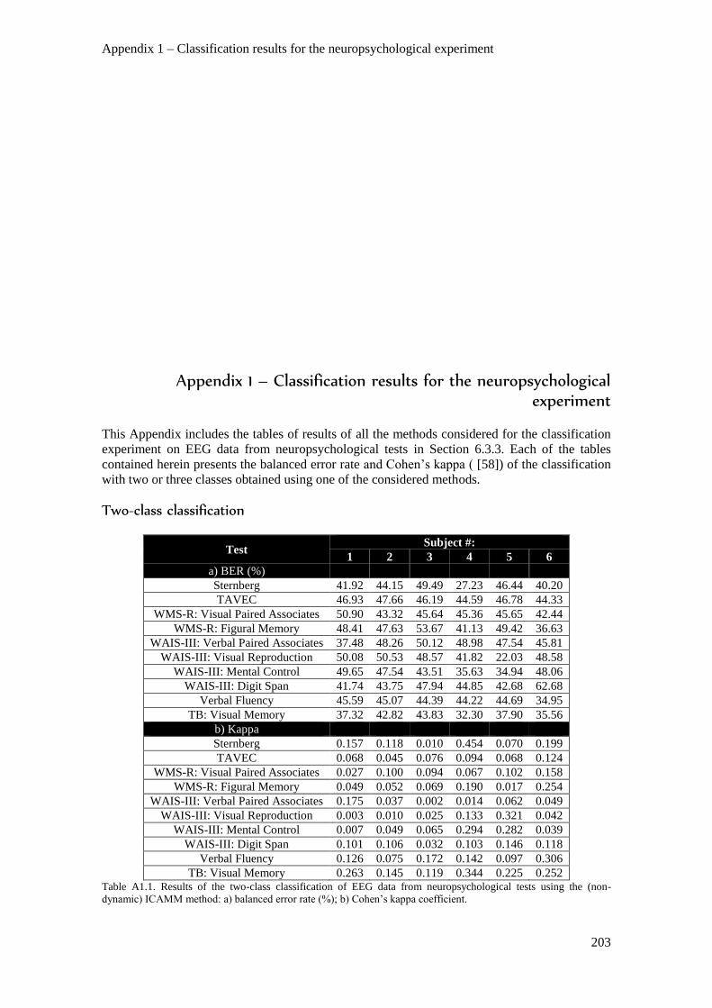
Appendix 1 – Classification results for the neuropsychological experiment
203
Appendix 1 – Classification results for the neuropsychological experiment
This Appendix includes the tables of results of all the methods considered for the classification
experiment on EEG data from neuropsychological tests in Section 6.3.3. Each of the tables
contained herein presents the balanced error rate and Cohen’s kappa ( [58]) of the classification
with two or three classes obtained using one of the considered methods.
Two-class classification
Test Subject #:
1 2 3 4 5 6
a) BER (%)
Sternberg 41.92 44.15 49.49 27.23 46.44 40.20
TAVEC 46.93 47.66 46.19 44.59 46.78 44.33
WMS-R: Visual Paired Associates 50.90 43.32 45.64 45.36 45.65 42.44
WMS-R: Figural Memory 48.41 47.63 53.67 41.13 49.42 36.63
WAIS-III: Verbal Paired Associates 37.48 48.26 50.12 48.98 47.54 45.81
WAIS-III: Visual Reproduction 50.08 50.53 48.57 41.82 22.03 48.58
WAIS-III: Mental Control 49.65 47.54 43.51 35.63 34.94 48.06
WAIS-III: Digit Span 41.74 43.75 47.94 44.85 42.68 62.68
Verbal Fluency 45.59 45.07 44.39 44.22 44.69 34.95
TB: Visual Memory 37.32 42.82 43.83 32.30 37.90 35.56
b) Kappa
Sternberg 0.157 0.118 0.010 0.454 0.070 0.199
TAVEC 0.068 0.045 0.076 0.094 0.068 0.124
WMS-R: Visual Paired Associates 0.027 0.100 0.094 0.067 0.102 0.158
WMS-R: Figural Memory 0.049 0.052 0.069 0.190 0.017 0.254
WAIS-III: Verbal Paired Associates 0.175 0.037 0.002 0.014 0.062 0.049
WAIS-III: Visual Reproduction 0.003 0.010 0.025 0.133 0.321 0.042
WAIS-III: Mental Control 0.007 0.049 0.065 0.294 0.282 0.039
WAIS-III: Digit Span 0.101 0.106 0.032 0.103 0.146 0.118
Verbal Fluency 0.126 0.075 0.172 0.142 0.097 0.306
TB: Visual Memory 0.263 0.145 0.119 0.344 0.225 0.252 Table A1.1. Results of the two-class classification of EEG data from neuropsychological tests using the (non-
dynamic) ICAMM method: a) balanced error rate (%); b) Cohen’s kappa coefficient.
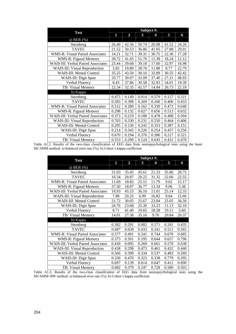
204
Test Subject #:
1 2 3 4 5 6
a) BER (%)
Sternberg 26.40 42.56 50.74 20.98 41.52 34.26
TAVEC 21.52 30.53 36.86 41.05 27.88 29.01
WMS-R: Visual Paired Associates 14.21 32.71 39.31 30.75 22.36 17.28
WMS-R: Figural Memory 38.72 41.65 51.76 11.38 18.24 12.12
WAIS-III: Verbal Paired Associates 23.44 39.68 39.18 17.60 32.97 16.98
WAIS-III: Visual Reproduction 5.82 19.80 28.76 11.88 8.77 22.79
WAIS-III: Mental Control 35.25 43.50 30.16 32.89 30.55 42.42
WAIS-III: Digit Span 33.77 30.07 32.09 37.40 27.21 48.93
Verbal Fluency 8.43 37.86 30.58 32.83 34.01 19.39
TB: Visual Memory 22.34 32.35 42.57 14.84 26.73 22.18
b) Kappa
Sternberg 0.475 0.149 0.014 0.579 0.157 0.321
TAVEC 0.583 0.398 0.269 0.160 0.406 0.433
WMS-R: Visual Paired Associates 0.512 0.280 0.162 0.330 0.473 0.648
WMS-R: Figural Memory 0.298 0.132 0.027 0.656 0.513 0.632
WAIS-III: Verbal Paired Associates 0.373 0.219 0.188 0.478 0.408 0.504
WAIS-III: Visual Reproduction 0.703 0.330 0.231 0.550 0.464 0.406
WAIS-III: Mental Control 0.295 0.130 0.245 0.353 0.387 0.151
WAIS-III: Digit Span 0.214 0.342 0.226 0.254 0.457 0.256
Verbal Fluency 0.670 0.194 0.376 0.386 0.217 0.521
TB: Visual Memory 0.553 0.299 0.124 0.643 0.431 0.470 Table A1.2. Results of the two-class classification of EEG data from neuropsychological tests using the basic
SICAMM method: a) balanced error rate (%); b) Cohen’s kappa coefficient.
Test Subject #:
1 2 3 4 5 6
a) BER (%)
Sternberg 31.03 35.45 45.61 21.33 35.86 28.75
TAVEC 16.54 20.87 29.22 31.32 22.66 22.55
WMS-R: Visual Paired Associates 11.69 18.82 25.51 11.79 9.65 15.17
WMS-R: Figural Memory 37.50 18.07 36.77 13.34 9.06 5.38
WAIS-III: Verbal Paired Associates 19.93 45.53 36.10 11.01 25.14 12.33
WAIS-III: Visual Reproduction 7.88 20.25 6.99 16.82 9.64 15.60
WAIS-III: Mental Control 21.72 30.05 25.67 23.84 25.05 36.50
WAIS-III: Digit Span 24.76 23.68 25.30 33.23 11.13 32.10
Verbal Fluency 8.71 41.40 19.65 18.38 19.11 5.60
TB: Visual Memory 14.01 27.36 35.16 9.76 20.84 20.37
b) Kappa
Sternberg 0.382 0.291 0.082 0.571 0.261 0.435
TAVEC 0.687 0.639 0.433 0.341 0.511 0.565
WMS-R: Visual Paired Associates 0.577 0.491 0.341 0.744 0.670 0.685
WMS-R: Figural Memory 0.373 0.501 0.195 0.644 0.657 0.796
WAIS-III: Verbal Paired Associates 0.439 0.095 0.269 0.661 0.570 0.638
WAIS-III: Visual Reproduction 0.438 0.298 0.473 0.461 0.432 0.440
WAIS-III: Mental Control 0.566 0.399 0.334 0.537 0.483 0.269
WAIS-III: Digit Span 0.330 0.470 0.323 0.338 0.779 0.295
Verbal Fluency 0.697 0.139 0.614 0.647 0.411 0.690
TB: Visual Memory 0.682 0.379 0.247 0.728 0.580 0.503 Table A1.3. Results of the two-class classification of EEG data from neuropsychological tests using the
SICAMM+BW method: a) balanced error rate (%); b) Cohen’s kappa coefficient.
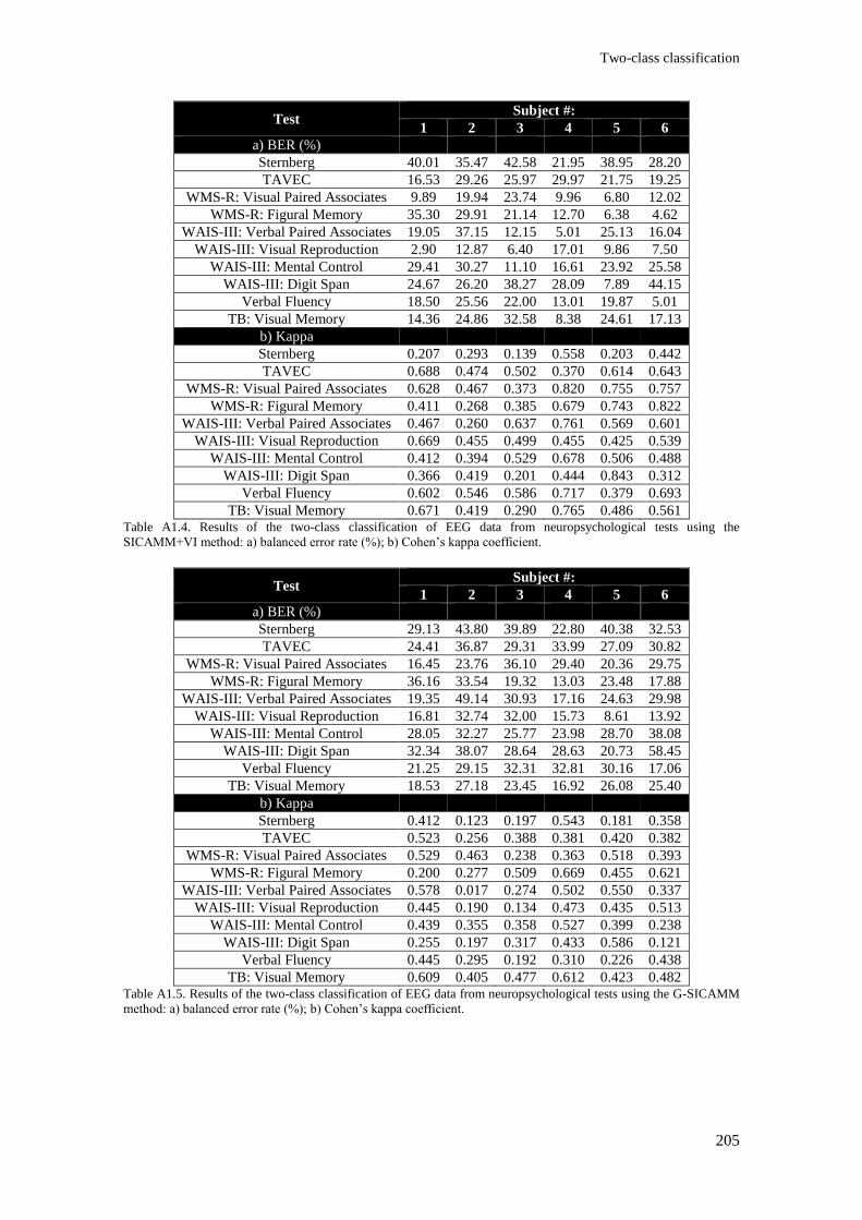
Two-class classification
205
Test Subject #:
1 2 3 4 5 6
a) BER (%)
Sternberg 40.01 35.47 42.58 21.95 38.95 28.20
TAVEC 16.53 29.26 25.97 29.97 21.75 19.25
WMS-R: Visual Paired Associates 9.89 19.94 23.74 9.96 6.80 12.02
WMS-R: Figural Memory 35.30 29.91 21.14 12.70 6.38 4.62
WAIS-III: Verbal Paired Associates 19.05 37.15 12.15 5.01 25.13 16.04
WAIS-III: Visual Reproduction 2.90 12.87 6.40 17.01 9.86 7.50
WAIS-III: Mental Control 29.41 30.27 11.10 16.61 23.92 25.58
WAIS-III: Digit Span 24.67 26.20 38.27 28.09 7.89 44.15
Verbal Fluency 18.50 25.56 22.00 13.01 19.87 5.01
TB: Visual Memory 14.36 24.86 32.58 8.38 24.61 17.13
b) Kappa
Sternberg 0.207 0.293 0.139 0.558 0.203 0.442
TAVEC 0.688 0.474 0.502 0.370 0.614 0.643
WMS-R: Visual Paired Associates 0.628 0.467 0.373 0.820 0.755 0.757
WMS-R: Figural Memory 0.411 0.268 0.385 0.679 0.743 0.822
WAIS-III: Verbal Paired Associates 0.467 0.260 0.637 0.761 0.569 0.601
WAIS-III: Visual Reproduction 0.669 0.455 0.499 0.455 0.425 0.539
WAIS-III: Mental Control 0.412 0.394 0.529 0.678 0.506 0.488
WAIS-III: Digit Span 0.366 0.419 0.201 0.444 0.843 0.312
Verbal Fluency 0.602 0.546 0.586 0.717 0.379 0.693
TB: Visual Memory 0.671 0.419 0.290 0.765 0.486 0.561 Table A1.4. Results of the two-class classification of EEG data from neuropsychological tests using the
SICAMM+VI method: a) balanced error rate (%); b) Cohen’s kappa coefficient.
Test Subject #:
1 2 3 4 5 6
a) BER (%)
Sternberg 29.13 43.80 39.89 22.80 40.38 32.53
TAVEC 24.41 36.87 29.31 33.99 27.09 30.82
WMS-R: Visual Paired Associates 16.45 23.76 36.10 29.40 20.36 29.75
WMS-R: Figural Memory 36.16 33.54 19.32 13.03 23.48 17.88
WAIS-III: Verbal Paired Associates 19.35 49.14 30.93 17.16 24.63 29.98
WAIS-III: Visual Reproduction 16.81 32.74 32.00 15.73 8.61 13.92
WAIS-III: Mental Control 28.05 32.27 25.77 23.98 28.70 38.08
WAIS-III: Digit Span 32.34 38.07 28.64 28.63 20.73 58.45
Verbal Fluency 21.25 29.15 32.31 32.81 30.16 17.06
TB: Visual Memory 18.53 27.18 23.45 16.92 26.08 25.40
b) Kappa
Sternberg 0.412 0.123 0.197 0.543 0.181 0.358
TAVEC 0.523 0.256 0.388 0.381 0.420 0.382
WMS-R: Visual Paired Associates 0.529 0.463 0.238 0.363 0.518 0.393
WMS-R: Figural Memory 0.200 0.277 0.509 0.669 0.455 0.621
WAIS-III: Verbal Paired Associates 0.578 0.017 0.274 0.502 0.550 0.337
WAIS-III: Visual Reproduction 0.445 0.190 0.134 0.473 0.435 0.513
WAIS-III: Mental Control 0.439 0.355 0.358 0.527 0.399 0.238
WAIS-III: Digit Span 0.255 0.197 0.317 0.433 0.586 0.121
Verbal Fluency 0.445 0.295 0.192 0.310 0.226 0.438
TB: Visual Memory 0.609 0.405 0.477 0.612 0.423 0.482 Table A1.5. Results of the two-class classification of EEG data from neuropsychological tests using the G-SICAMM
method: a) balanced error rate (%); b) Cohen’s kappa coefficient.
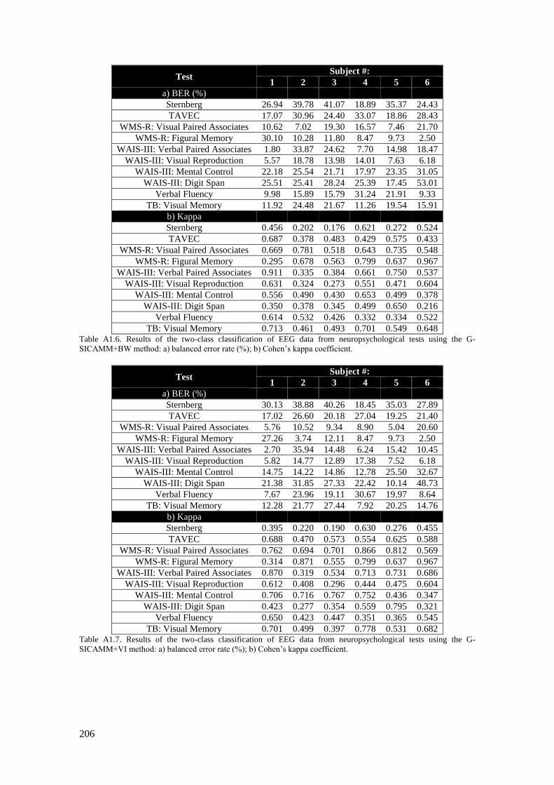
206
Test Subject #:
1 2 3 4 5 6
a) BER (%)
Sternberg 26.94 39.78 41.07 18.89 35.37 24.43
TAVEC 17.07 30.96 24.40 33.07 18.86 28.43
WMS-R: Visual Paired Associates 10.62 7.02 19.30 16.57 7.46 21.70
WMS-R: Figural Memory 30.10 10.28 11.80 8.47 9.73 2.50
WAIS-III: Verbal Paired Associates 1.80 33.87 24.62 7.70 14.98 18.47
WAIS-III: Visual Reproduction 5.57 18.78 13.98 14.01 7.63 6.18
WAIS-III: Mental Control 22.18 25.54 21.71 17.97 23.35 31.05
WAIS-III: Digit Span 25.51 25.41 28.24 25.39 17.45 53.01
Verbal Fluency 9.98 15.89 15.79 31.24 21.91 9.33
TB: Visual Memory 11.92 24.48 21.67 11.26 19.54 15.91
b) Kappa
Sternberg 0.456 0.202 0.176 0.621 0.272 0.524
TAVEC 0.687 0.378 0.483 0.429 0.575 0.433
WMS-R: Visual Paired Associates 0.669 0.781 0.518 0.643 0.735 0.548
WMS-R: Figural Memory 0.295 0.678 0.563 0.799 0.637 0.967
WAIS-III: Verbal Paired Associates 0.911 0.335 0.384 0.661 0.750 0.537
WAIS-III: Visual Reproduction 0.631 0.324 0.273 0.551 0.471 0.604
WAIS-III: Mental Control 0.556 0.490 0.430 0.653 0.499 0.378
WAIS-III: Digit Span 0.350 0.378 0.345 0.499 0.650 0.216
Verbal Fluency 0.614 0.532 0.426 0.332 0.334 0.522
TB: Visual Memory 0.713 0.461 0.493 0.701 0.549 0.648 Table A1.6. Results of the two-class classification of EEG data from neuropsychological tests using the G-
SICAMM+BW method: a) balanced error rate (%); b) Cohen’s kappa coefficient.
Test Subject #:
1 2 3 4 5 6
a) BER (%)
Sternberg 30.13 38.88 40.26 18.45 35.03 27.89
TAVEC 17.02 26.60 20.18 27.04 19.25 21.40
WMS-R: Visual Paired Associates 5.76 10.52 9.34 8.90 5.04 20.60
WMS-R: Figural Memory 27.26 3.74 12.11 8.47 9.73 2.50
WAIS-III: Verbal Paired Associates 2.70 35.94 14.48 6.24 15.42 10.45
WAIS-III: Visual Reproduction 5.82 14.77 12.89 17.38 7.52 6.18
WAIS-III: Mental Control 14.75 14.22 14.86 12.78 25.50 32.67
WAIS-III: Digit Span 21.38 31.85 27.33 22.42 10.14 48.73
Verbal Fluency 7.67 23.96 19.11 30.67 19.97 8.64
TB: Visual Memory 12.28 21.77 27.44 7.92 20.25 14.76
b) Kappa
Sternberg 0.395 0.220 0.190 0.630 0.276 0.455
TAVEC 0.688 0.470 0.573 0.554 0.625 0.588
WMS-R: Visual Paired Associates 0.762 0.694 0.701 0.866 0.812 0.569
WMS-R: Figural Memory 0.314 0.871 0.555 0.799 0.637 0.967
WAIS-III: Verbal Paired Associates 0.870 0.319 0.534 0.713 0.731 0.686
WAIS-III: Visual Reproduction 0.612 0.408 0.296 0.444 0.475 0.604
WAIS-III: Mental Control 0.706 0.716 0.767 0.752 0.436 0.347
WAIS-III: Digit Span 0.423 0.277 0.354 0.559 0.795 0.321
Verbal Fluency 0.650 0.423 0.447 0.351 0.365 0.545
TB: Visual Memory 0.701 0.499 0.397 0.778 0.531 0.682 Table A1.7. Results of the two-class classification of EEG data from neuropsychological tests using the G-
SICAMM+VI method: a) balanced error rate (%); b) Cohen’s kappa coefficient.
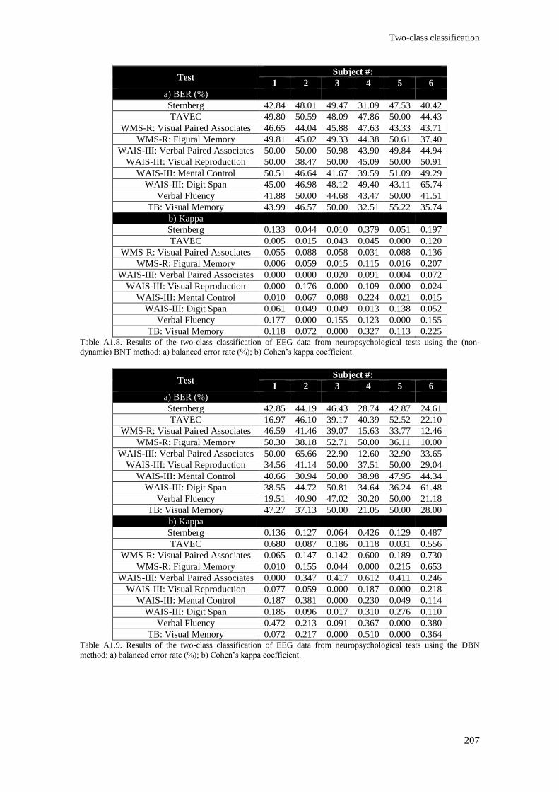
Two-class classification
207
Test Subject #:
1 2 3 4 5 6
a) BER (%)
Sternberg 42.84 48.01 49.47 31.09 47.53 40.42
TAVEC 49.80 50.59 48.09 47.86 50.00 44.43
WMS-R: Visual Paired Associates 46.65 44.04 45.88 47.63 43.33 43.71
WMS-R: Figural Memory 49.81 45.02 49.33 44.38 50.61 37.40
WAIS-III: Verbal Paired Associates 50.00 50.00 50.98 43.90 49.84 44.94
WAIS-III: Visual Reproduction 50.00 38.47 50.00 45.09 50.00 50.91
WAIS-III: Mental Control 50.51 46.64 41.67 39.59 51.09 49.29
WAIS-III: Digit Span 45.00 46.98 48.12 49.40 43.11 65.74
Verbal Fluency 41.88 50.00 44.68 43.47 50.00 41.51
TB: Visual Memory 43.99 46.57 50.00 32.51 55.22 35.74
b) Kappa
Sternberg 0.133 0.044 0.010 0.379 0.051 0.197
TAVEC 0.005 0.015 0.043 0.045 0.000 0.120
WMS-R: Visual Paired Associates 0.055 0.088 0.058 0.031 0.088 0.136
WMS-R: Figural Memory 0.006 0.059 0.015 0.115 0.016 0.207
WAIS-III: Verbal Paired Associates 0.000 0.000 0.020 0.091 0.004 0.072
WAIS-III: Visual Reproduction 0.000 0.176 0.000 0.109 0.000 0.024
WAIS-III: Mental Control 0.010 0.067 0.088 0.224 0.021 0.015
WAIS-III: Digit Span 0.061 0.049 0.049 0.013 0.138 0.052
Verbal Fluency 0.177 0.000 0.155 0.123 0.000 0.155
TB: Visual Memory 0.118 0.072 0.000 0.327 0.113 0.225 Table A1.8. Results of the two-class classification of EEG data from neuropsychological tests using the (non-
dynamic) BNT method: a) balanced error rate (%); b) Cohen’s kappa coefficient.
Test Subject #:
1 2 3 4 5 6
a) BER (%)
Sternberg 42.85 44.19 46.43 28.74 42.87 24.61
TAVEC 16.97 46.10 39.17 40.39 52.52 22.10
WMS-R: Visual Paired Associates 46.59 41.46 39.07 15.63 33.77 12.46
WMS-R: Figural Memory 50.30 38.18 52.71 50.00 36.11 10.00
WAIS-III: Verbal Paired Associates 50.00 65.66 22.90 12.60 32.90 33.65
WAIS-III: Visual Reproduction 34.56 41.14 50.00 37.51 50.00 29.04
WAIS-III: Mental Control 40.66 30.94 50.00 38.98 47.95 44.34
WAIS-III: Digit Span 38.55 44.72 50.81 34.64 36.24 61.48
Verbal Fluency 19.51 40.90 47.02 30.20 50.00 21.18
TB: Visual Memory 47.27 37.13 50.00 21.05 50.00 28.00
b) Kappa
Sternberg 0.136 0.127 0.064 0.426 0.129 0.487
TAVEC 0.680 0.087 0.186 0.118 0.031 0.556
WMS-R: Visual Paired Associates 0.065 0.147 0.142 0.600 0.189 0.730
WMS-R: Figural Memory 0.010 0.155 0.044 0.000 0.215 0.653
WAIS-III: Verbal Paired Associates 0.000 0.347 0.417 0.612 0.411 0.246
WAIS-III: Visual Reproduction 0.077 0.059 0.000 0.187 0.000 0.218
WAIS-III: Mental Control 0.187 0.381 0.000 0.230 0.049 0.114
WAIS-III: Digit Span 0.185 0.096 0.017 0.310 0.276 0.110
Verbal Fluency 0.472 0.213 0.091 0.367 0.000 0.380
TB: Visual Memory 0.072 0.217 0.000 0.510 0.000 0.364 Table A1.9. Results of the two-class classification of EEG data from neuropsychological tests using the DBN
method: a) balanced error rate (%); b) Cohen’s kappa coefficient.
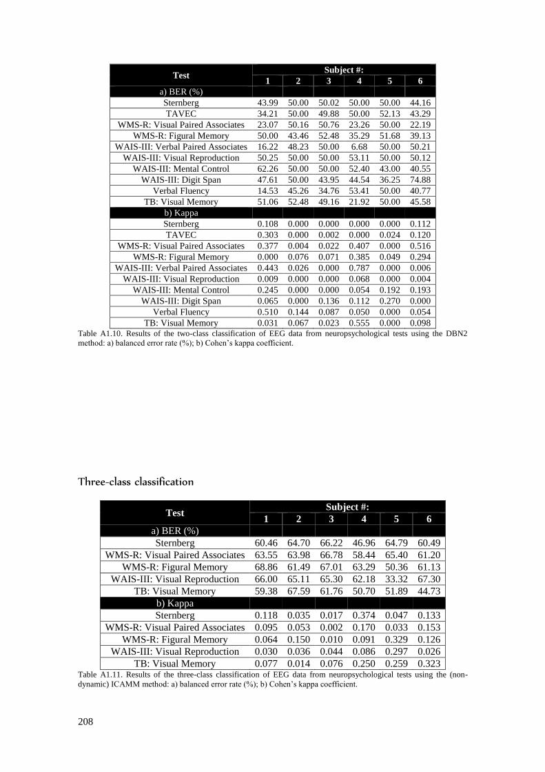
208
Test Subject #:
1 2 3 4 5 6
a) BER (%)
Sternberg 43.99 50.00 50.02 50.00 50.00 44.16
TAVEC 34.21 50.00 49.88 50.00 52.13 43.29
WMS-R: Visual Paired Associates 23.07 50.16 50.76 23.26 50.00 22.19
WMS-R: Figural Memory 50.00 43.46 52.48 35.29 51.68 39.13
WAIS-III: Verbal Paired Associates 16.22 48.23 50.00 6.68 50.00 50.21
WAIS-III: Visual Reproduction 50.25 50.00 50.00 53.11 50.00 50.12
WAIS-III: Mental Control 62.26 50.00 50.00 52.40 43.00 40.55
WAIS-III: Digit Span 47.61 50.00 43.95 44.54 36.25 74.88
Verbal Fluency 14.53 45.26 34.76 53.41 50.00 40.77
TB: Visual Memory 51.06 52.48 49.16 21.92 50.00 45.58
b) Kappa
Sternberg 0.108 0.000 0.000 0.000 0.000 0.112
TAVEC 0.303 0.000 0.002 0.000 0.024 0.120
WMS-R: Visual Paired Associates 0.377 0.004 0.022 0.407 0.000 0.516
WMS-R: Figural Memory 0.000 0.076 0.071 0.385 0.049 0.294
WAIS-III: Verbal Paired Associates 0.443 0.026 0.000 0.787 0.000 0.006
WAIS-III: Visual Reproduction 0.009 0.000 0.000 0.068 0.000 0.004
WAIS-III: Mental Control 0.245 0.000 0.000 0.054 0.192 0.193
WAIS-III: Digit Span 0.065 0.000 0.136 0.112 0.270 0.000
Verbal Fluency 0.510 0.144 0.087 0.050 0.000 0.054
TB: Visual Memory 0.031 0.067 0.023 0.555 0.000 0.098 Table A1.10. Results of the two-class classification of EEG data from neuropsychological tests using the DBN2
method: a) balanced error rate (%); b) Cohen’s kappa coefficient.
Three-class classification
Test Subject #:
1 2 3 4 5 6
a) BER (%)
Sternberg 60.46 64.70 66.22 46.96 64.79 60.49
WMS-R: Visual Paired Associates 63.55 63.98 66.78 58.44 65.40 61.20
WMS-R: Figural Memory 68.86 61.49 67.01 63.29 50.36 61.13
WAIS-III: Visual Reproduction 66.00 65.11 65.30 62.18 33.32 67.30
TB: Visual Memory 59.38 67.59 61.76 50.70 51.89 44.73
b) Kappa
Sternberg 0.118 0.035 0.017 0.374 0.047 0.133
WMS-R: Visual Paired Associates 0.095 0.053 0.002 0.170 0.033 0.153
WMS-R: Figural Memory 0.064 0.150 0.010 0.091 0.329 0.126
WAIS-III: Visual Reproduction 0.030 0.036 0.044 0.086 0.297 0.026
TB: Visual Memory 0.077 0.014 0.076 0.250 0.259 0.323 Table A1.11. Results of the three-class classification of EEG data from neuropsychological tests using the (non-
dynamic) ICAMM method: a) balanced error rate (%); b) Cohen’s kappa coefficient.
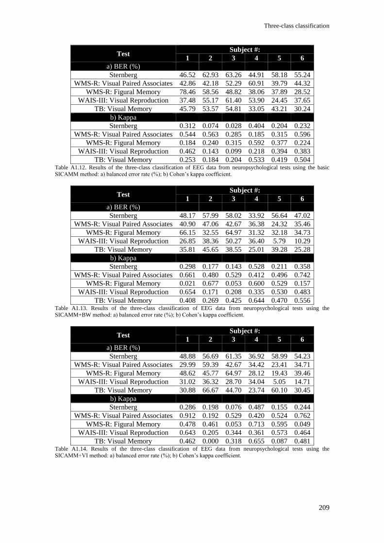
Three-class classification
209
Test Subject #:
1 2 3 4 5 6
a) BER (%)
Sternberg 46.52 62.93 63.26 44.91 58.18 55.24
WMS-R: Visual Paired Associates 42.86 42.18 52.29 60.91 39.79 44.32
WMS-R: Figural Memory 78.46 58.56 48.82 38.06 37.89 28.52
WAIS-III: Visual Reproduction 37.48 55.17 61.40 53.90 24.45 37.65
TB: Visual Memory 45.79 53.57 54.81 33.05 43.21 30.24
b) Kappa
Sternberg 0.312 0.074 0.028 0.404 0.204 0.232
WMS-R: Visual Paired Associates 0.544 0.563 0.285 0.185 0.315 0.596
WMS-R: Figural Memory 0.184 0.240 0.315 0.592 0.377 0.224
WAIS-III: Visual Reproduction 0.462 0.143 0.099 0.218 0.394 0.383
TB: Visual Memory 0.253 0.184 0.204 0.533 0.419 0.504 Table A1.12. Results of the three-class classification of EEG data from neuropsychological tests using the basic
SICAMM method: a) balanced error rate (%); b) Cohen’s kappa coefficient.
Test Subject #:
1 2 3 4 5 6
a) BER (%)
Sternberg 48.17 57.99 58.02 33.92 56.64 47.02
WMS-R: Visual Paired Associates 40.90 47.06 42.67 36.38 24.32 35.46
WMS-R: Figural Memory 66.15 32.55 64.97 31.32 32.18 34.73
WAIS-III: Visual Reproduction 26.85 38.36 50.27 36.40 5.79 10.29
TB: Visual Memory 35.81 45.65 38.55 25.01 39.28 25.28
b) Kappa
Sternberg 0.298 0.177 0.143 0.528 0.211 0.358
WMS-R: Visual Paired Associates 0.661 0.480 0.529 0.412 0.496 0.742
WMS-R: Figural Memory 0.021 0.677 0.053 0.600 0.529 0.157
WAIS-III: Visual Reproduction 0.654 0.171 0.208 0.335 0.530 0.483
TB: Visual Memory 0.408 0.269 0.425 0.644 0.470 0.556 Table A1.13. Results of the three-class classification of EEG data from neuropsychological tests using the
SICAMM+BW method: a) balanced error rate (%); b) Cohen’s kappa coefficient.
Test Subject #:
1 2 3 4 5 6
a) BER (%)
Sternberg 48.88 56.69 61.35 36.92 58.99 54.23
WMS-R: Visual Paired Associates 29.99 59.39 42.67 34.42 23.41 34.71
WMS-R: Figural Memory 48.62 45.77 64.97 28.12 19.43 39.46
WAIS-III: Visual Reproduction 31.02 36.32 28.70 34.04 5.05 14.71
TB: Visual Memory 30.88 66.67 44.70 23.74 60.10 30.45
b) Kappa
Sternberg 0.286 0.198 0.076 0.487 0.155 0.244
WMS-R: Visual Paired Associates 0.912 0.192 0.529 0.420 0.524 0.762
WMS-R: Figural Memory 0.478 0.461 0.053 0.713 0.595 0.049
WAIS-III: Visual Reproduction 0.643 0.205 0.344 0.361 0.573 0.464
TB: Visual Memory 0.462 0.000 0.318 0.655 0.087 0.481 Table A1.14. Results of the three-class classification of EEG data from neuropsychological tests using the
SICAMM+VI method: a) balanced error rate (%); b) Cohen’s kappa coefficient.
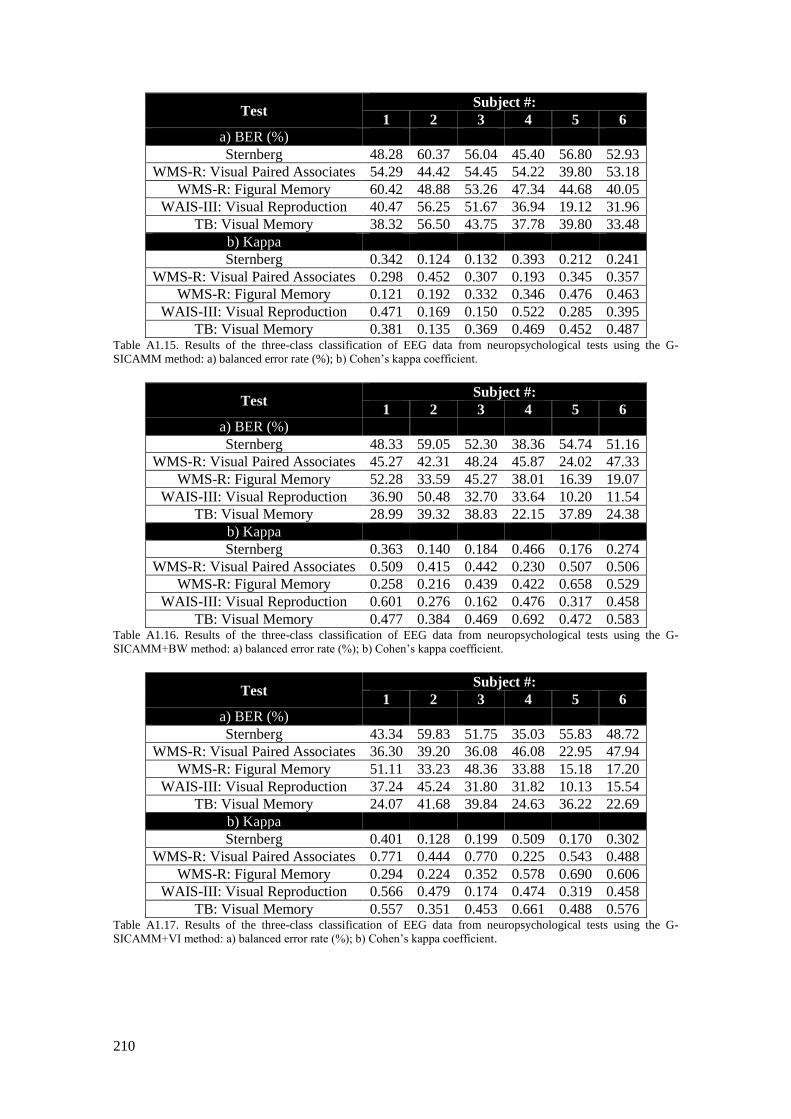
210
Test Subject #:
1 2 3 4 5 6
a) BER (%)
Sternberg 48.28 60.37 56.04 45.40 56.80 52.93
WMS-R: Visual Paired Associates 54.29 44.42 54.45 54.22 39.80 53.18
WMS-R: Figural Memory 60.42 48.88 53.26 47.34 44.68 40.05
WAIS-III: Visual Reproduction 40.47 56.25 51.67 36.94 19.12 31.96
TB: Visual Memory 38.32 56.50 43.75 37.78 39.80 33.48
b) Kappa
Sternberg 0.342 0.124 0.132 0.393 0.212 0.241
WMS-R: Visual Paired Associates 0.298 0.452 0.307 0.193 0.345 0.357
WMS-R: Figural Memory 0.121 0.192 0.332 0.346 0.476 0.463
WAIS-III: Visual Reproduction 0.471 0.169 0.150 0.522 0.285 0.395
TB: Visual Memory 0.381 0.135 0.369 0.469 0.452 0.487 Table A1.15. Results of the three-class classification of EEG data from neuropsychological tests using the G-
SICAMM method: a) balanced error rate (%); b) Cohen’s kappa coefficient.
Test Subject #:
1 2 3 4 5 6
a) BER (%)
Sternberg 48.33 59.05 52.30 38.36 54.74 51.16
WMS-R: Visual Paired Associates 45.27 42.31 48.24 45.87 24.02 47.33
WMS-R: Figural Memory 52.28 33.59 45.27 38.01 16.39 19.07
WAIS-III: Visual Reproduction 36.90 50.48 32.70 33.64 10.20 11.54
TB: Visual Memory 28.99 39.32 38.83 22.15 37.89 24.38
b) Kappa
Sternberg 0.363 0.140 0.184 0.466 0.176 0.274
WMS-R: Visual Paired Associates 0.509 0.415 0.442 0.230 0.507 0.506
WMS-R: Figural Memory 0.258 0.216 0.439 0.422 0.658 0.529
WAIS-III: Visual Reproduction 0.601 0.276 0.162 0.476 0.317 0.458
TB: Visual Memory 0.477 0.384 0.469 0.692 0.472 0.583 Table A1.16. Results of the three-class classification of EEG data from neuropsychological tests using the G-
SICAMM+BW method: a) balanced error rate (%); b) Cohen’s kappa coefficient.
Test Subject #:
1 2 3 4 5 6
a) BER (%)
Sternberg 43.34 59.83 51.75 35.03 55.83 48.72
WMS-R: Visual Paired Associates 36.30 39.20 36.08 46.08 22.95 47.94
WMS-R: Figural Memory 51.11 33.23 48.36 33.88 15.18 17.20
WAIS-III: Visual Reproduction 37.24 45.24 31.80 31.82 10.13 15.54
TB: Visual Memory 24.07 41.68 39.84 24.63 36.22 22.69
b) Kappa
Sternberg 0.401 0.128 0.199 0.509 0.170 0.302
WMS-R: Visual Paired Associates 0.771 0.444 0.770 0.225 0.543 0.488
WMS-R: Figural Memory 0.294 0.224 0.352 0.578 0.690 0.606
WAIS-III: Visual Reproduction 0.566 0.479 0.174 0.474 0.319 0.458
TB: Visual Memory 0.557 0.351 0.453 0.661 0.488 0.576 Table A1.17. Results of the three-class classification of EEG data from neuropsychological tests using the G-
SICAMM+VI method: a) balanced error rate (%); b) Cohen’s kappa coefficient.
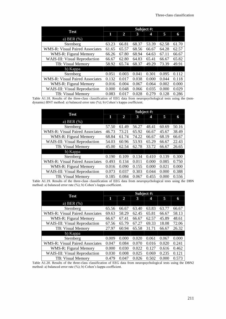
Three-class classification
211
Test Subject #:
1 2 3 4 5 6
a) BER (%)
Sternberg 63.23 66.81 68.37 53.39 62.58 61.70
WMS-R: Visual Paired Associates 61.65 65.57 68.56 66.67 64.28 62.57
WMS-R: Figural Memory 66.26 67.80 68.94 64.63 67.11 66.67
WAIS-III: Visual Reproduction 66.67 62.80 64.83 65.41 66.67 65.82
TB: Visual Memory 58.92 65.74 68.37 49.29 73.39 49.91
b) Kappa
Sternberg 0.051 0.003 0.041 0.301 0.095 0.112
WMS-R: Visual Paired Associates 0.132 0.017 0.038 0.000 0.044 0.118
WMS-R: Figural Memory 0.016 0.004 0.067 0.064 0.002 0.000
WAIS-III: Visual Reproduction 0.000 0.048 0.066 0.035 0.000 0.029
TB: Visual Memory 0.083 0.017 0.028 0.279 0.128 0.286 Table A1.18. Results of the three-class classification of EEG data from neuropsychological tests using the (non-
dynamic) BNT method: a) balanced error rate (%); b) Cohen’s kappa coefficient.
Test Subject #:
1 2 3 4 5 6
a) BER (%)
Sternberg 57.50 61.49 56.27 48.41 60.69 50.16
WMS-R: Visual Paired Associates 46.73 73.21 65.92 66.67 45.67 38.49
WMS-R: Figural Memory 68.84 61.74 74.22 66.67 68.19 66.67
WAIS-III: Visual Reproduction 54.03 60.96 53.93 65.29 66.67 22.43
TB: Visual Memory 45.00 62.54 62.78 33.72 66.67 26.65
b) Kappa
Sternberg 0.190 0.109 0.134 0.410 0.139 0.300
WMS-R: Visual Paired Associates 0.493 0.134 0.011 0.000 0.085 0.750
WMS-R: Figural Memory 0.016 0.090 0.155 0.000 0.021 0.000
WAIS-III: Visual Reproduction 0.073 0.037 0.303 0.044 0.000 0.388
TB: Visual Memory 0.185 0.084 0.067 0.455 0.000 0.556 Table A1.19. Results of the three-class classification of EEG data from neuropsychological tests using the DBN
method: a) balanced error rate (%); b) Cohen’s kappa coefficient.
Test Subject #:
1 2 3 4 5 6
a) BER (%)
Sternberg 65.56 66.67 63.40 63.83 63.77 66.67
WMS-R: Visual Paired Associates 69.63 58.29 62.45 65.81 66.67 58.13
WMS-R: Figural Memory 66.67 67.41 66.67 62.57 45.89 48.61
WAIS-III: Visual Reproduction 67.56 65.79 67.27 69.33 18.08 72.06
TB: Visual Memory 27.97 60.94 65.58 31.71 66.67 26.32
b) Kappa
Sternberg 0.009 0.000 0.020 0.061 0.067 0.000
WMS-R: Visual Paired Associates 0.047 0.084 0.070 0.016 0.020 0.241
WMS-R: Figural Memory 0.000 0.030 0.022 0.127 0.616 0.462
WAIS-III: Visual Reproduction 0.030 0.008 0.025 0.069 0.235 0.121
TB: Visual Memory 0.479 0.047 0.026 0.502 0.000 0.573 Table A1.20. Results of the three-class classification of EEG data from neuropsychological tests using the DBN2
method: a) balanced error rate (%); b) Cohen’s kappa coefficient.


213
References

215
References [1] P.B. Adelman and S.A. Vogel, "College Graduates with Learning Disabilities:
Employment Attainment and Career Patterns," Learning Disability Quaterly, vol. 13, no.
3, pp. 154-166, 1990.
[2] R. Agarwal and J. Gotman, "Computer-assisted sleep staging," IEEE Transactions on
Biomedical Engineering, vol. 48, no. 12, pp. 1412-1423, 2001.
[3] P. Aguilera, A. Fernandez, R. Ropero, and L. Molina, "Groundwater quality assessment
using data clustering based on hybrid Bayesian networks," Stochastic Environmental
Research and Risk Assessment, vol. 27, pp. 435-447, 2013.
[4] H. Akaike, "A new look at the statistical model identification," IEEE Transactions on
Automatic Control, vol. 19, no. 6, pp. 716-723, 1974.
[5] A.M. Alattar, E.T. Lin, and M.U. Celik, "Digital watermarking of low bit-rate advanced
simple profile MPEG-4 campressed video," IEEE Transactions on Circuits and Systems
for Video Technology, vol. 13, no. 8, pp. 787-800, 2003.
[6] D. Alfè, M.J Gillan, and G.D Price, "Composition and temperature of the Earth’s core
constrained by combining ab initio calculations and seismic data," Earth and Planetary
Science Letters, vol. 195, no. 1-2, pp. 91-98, 2002.
[7] S.I. Amari, "Natural Gradient Works Efficiently in Learning," Neural Computation, vol.
10, pp. 251-276, 1998.
[8] S. Amari and J.F. Cardoso, "Blind source separation-semiparametric statistical approach,"
IEEE Transactions on Signal Processing, vol. 45, no. 11, pp. 2692-2700, 1997.
[9] S. Amari, A. Chichocki, and H.H Yang, "A new learning algorithm for blind source
separation," Proceedings Advances in Neural Information Processing Systems, pp. 757-
763, 1996.
[10] L. Amini, C. Jutten, B. Pouyatos, A. Depaulis, and C. Roucard, "Dynamical Analysis of
Brain Seizure Activity from EEG Signals," in 22nd European Signal Processing
Conference (EUSIPCO), Lisbon (Portugal), 2014, pp. 1-5.
[11] A. Anandkumar, R. Ge, D. Hsu, S.M. Kakade, and M. Telgarsky, "Tensor decompositions
for learning latent variable models," Journal of Machine Learning Research, vol. 15, pp.
2773-2832, 2014.
[12] C. Archambeau, N. Delannay, and M. Verleysen, "Mixtures of robust probabilistic
principal component analyzers," Neurocomputing, vol. 71, no. 7-9, pp. 1274-1282, 2008.
216
[13] A.D. Baddeley, Working Memory, Thought, and Action. UK: Oxford University Press,
2007.
[14] A. Banerjee, I. S. Dhillon, J. Ghosh, and S. Sra, "Clustering on the unit hypesphere using
von Mises-Fisher distributions," Journal of Machine Learning Research, vol. 6, pp. 1345-
1382, 2005.
[15] P. Barbillon, G. Celeux, A. Grimaud, Y. Lefebvre, and E. De Rochquigny, "Nonlinear
methods for inverse statistical problems," Computational Statistics & Data Analysis, vol.
55, pp. 132-142, 2011.
[16] M.S. Bartlett, J.R. Movellan, and T.J. Sejnowski, "Face recognition by independent
component analysis," IEEE Transactions on Neural Networks, vol. 13, no. 6, pp. 1450-
1464, 2002.
[17] L.E. Baum, T. Petrie, G. Soules, and N. Weiss, "A Maximization Technique Occurring in
the Statistical Analysis of Probabilistic Functions of Markov Chains," Annals of
Mathematical Statistics, vol. 41, no. 1, pp. 164-171, 1970.
[18] T. Bedford and R. Cooke, "Probability Density Decomposition for Conditionally
Dependent Random Variables Modeled by Vines," Annals of Mathematics and Artificial
Intelligence, vol. 32, no. 1, pp. 245-268, 2001.
[19] A.J. Bell and T.J. Sejnowski, "The "indendent components" of natural scenes are edge
filters," Vision Research, vol. 37, no. 23, pp. 3327-3338, 1997.
[20] M.J. Benedet and M.A. Alejandre, Test de Aprendizaje Verbal España-Complutense.
Spain: TEA Ediciones, 1998.
[21] L. Bentabet, S. Jodouin, D. Ziou, and J. Vaillancourt, "Road vectors update using SAR
imagery: A snake-based method," IEEE Transactions on Geoscience and Remote Sensing,
vol. 41, pp. 1785-1803, 2003.
[22] J. M. Bernardo and A.F.M. Smith, Bayesian Theory.: Wiley, 1994.
[23] J. Berryman, "Approximate methods for time‐reversal processing of large seismic
reflection data sets," Journal of the Accoustical Society of America, vol. 115, no. 5, pp.
2471-2471, 2004.
[24] D. Bersektas, Nonlinear programming. Belmont, MA, USA: Athena Scientific, 1999.
[25] J.C. Bezdek and S.K. Pal, Fuzzy Models for Pattern Recognition: Methods that Search for
Structures in Data. New York, USA: IEEE Press, 1992.
[26] C.M. Bishop, Pattern Recognition and Machine Learning. New York, USA: Springer,
2006.
[27] D. M. Blei, "Build, compute, critique, repeat: Data analysis with latent variable models,"
Annual Review of Statistics and Its Application, vol. 1, pp. 203-232, 2014.
[28] D. Borsboom, "Latent variable theory," Measurement, vol. 6, pp. 25-53, 2008.
[29] D. Bouchaffra, "Nonlinear Topological Component Analysis: Application to Age-
Invariant Face Recognition," IEEE Transactions on Neural Networks and Learning
Systems, to appear in 2015.
[30] M. Boutayeb and M. Darouach, "Recursive identification method for MISO Wiener-
Hammerstein model," IEEE Transactions on Automatic Control, vol. 40, pp. 287-291,
1995.
[31] E. Bouyé, V. Durrleman, A. Nikeghbali, G. Riboulet, and T. Roncalli, Copulas for
finance - A reading guide and some applications.: SSRN eLibrary, 2000.
[32] M. Brand, "Coupled hidden Markov models for modeling interacting processes," 1997.
[33] S.P. Brooks, "On Bayesian analyses and finite mixtures for proportions," Statistics and
Computing, vol. 11, pp. 179-190, 2001.
[34] R. Cabeza and L. Nyberg, "Imaging cognition II: An empirical review of 275 PET and
fMRI studies," Journal of Cognitive Neuroscience, vol. 12, pp. 1-47, 2000.
217
[35] C.F. Caiafa, E. Salerno, and A.N. Proto, "Blind Source Separation Applied to Spectral
Unmixing: Comparing Different Measures of Nongaussianity," Lecture Notes in
Computer Science, vol. 4694, pp. 1-8, 2007.
[36] E.J. Candès and B. Recht, "Exact Matrix Completion via Convex Optimization,"
Foundations of Computational Mathematics, vol. 9, no. 6, pp. 717-722, 2009.
[37] J.V. Candy, "Bootstrap particle filtering," IEEE Signal Processing Magazine, vol. 24, no.
4, pp. 73-85, 2007.
[38] J. Cao and W. Yao, "Semiparametric mixture of binomial regression with a degenerate
component," Statistica Sinica, vol. 22, no. 1, pp. 27-46, 2012.
[39] O. Cappe, E. Moulines, and T. Ryden, Inference in Hidden Markov Models. New York,
NY: Springer, 2005.
[40] J.F. Cardoso, "Blind signal separation: statistical principles," Proceedings of the IEEE,
Special Issue on Blind Identification and Estimation, vol. 9, pp. 2009-2025, 1998.
[41] Jean Carletta, "Assessing agreement on classification tasks: The kappa statistic,"
Computational Linguistics, vol. 22, no. 2, pp. 249-254, 1996.
[42] R. J. Carroll, D. Ruppert, L. A. Stefanski, and C. M. Crainiceanu, Measurement error in
nonlinear models: a modern perspective. Boca Raton, FL, USA: Chapman & Hall/CRC,
2006.
[43] N.J. Cassidy, "Ground penetrating radar data processing, modelling and analysis," in
Ground Penetrating Radar Theory and Applications.: Elsevier, 2009, pp. 141-176.
[44] N.P. Castellanos and V.A. Makarov, "Recovering EEG brain signals: Artifact suppression
with wavelet enhanced independent component analysis," Journal of Neuroscience
Methods, vol. 158, pp. 300-312, 2006.
[45] H.E. Cekli and H. Gunes, "Spatial resolution enhancement and reconstruction of mixed
convection data using kriging method," in ASME International Mechanical Engineering
Congress and Exposition, Chicago, IL, USA, 2006, pp. 447-456.
[46] J.C.C. Chan and A.L. Grant, "Fast computation of the deviance information creiterion for
latent variable models," Computational Statistics and Dats Analysis, to appear in 2015.
[47] A. Chan, E. Halgren, K. Marinkovic, and S. Cash, "Decoding word and category-specific
spatiotemporal representations from MEG and EEG," Neuroimage, vol. 54, no. 4, pp.
3028-3039, 2011.
[48] K. Chan, T.W. Lee, and T.J. Sejnowski, "Variational learning of clusters of
undercomplete nonsymmetric independent components," Journal of Machine Learning
Research, vol. 3, pp. 99-114, 2002.
[49] F.H.I. Chan and R. Luus, "A non-iterative method for identification using Hammerstein
model," IEEE Transactions on Automatic Control, vol. 16, pp. 464-468, 1971.
[50] O. Chapelle, B. Schölkopf, and A. Zien, Semi-supervised Learning. Cambridge (MA),
USA: MIT Press, 2006.
[51] W.G. Chase and K.A. Ericsson, "Skill and working memory," The Psychology of
Learning and Motivation, vol. 16, pp. 1-58, 1982.
[52] N. Cheng and J. Zhu, "Learning harmonium models with infinite latent features," IEEE
Transactions on Neural Networks and Learning Systems, vol. 25, no. 3, pp. 520-532,
2014.
[53] R. Chen and J.S. Lui, "Mixture Kalman filters," Journal of the Royal Statistical Society:
Series B, vol. 62, pp. 493-508, 2000.
[54] R. Choudrey and S. Roberts, "Variational mixture of bayesian independent component
analysers," Neural Computation, vol. 15, no. 1, pp. 213-252, 2002.
[55] A. Cichocki and S. Amari, Adaptive Blind Signal and Image Processing: Learning
algorithms and applications. New York, USA: Wiley, John & Sons, 2001.
[56] A. Cichocki, R. Zdunek, A.H. Phan, and S. Amari, Nonnegative Matrix and Tensor
218
Factorizations: Applications to Exploratory Multi-way Data Analysis and Blind Source
Separation.: John Wiley, 2009.
[57] B. R. Cobb and P. P. Shenoy, "Inference in hybrid Bayesian networks with mixtures of
truncated exponentials," International Journal of Approximate Reasoning, vol. 41, no. 3,
pp. 257-286, 2006.
[58] Jacob Cohen, "A coefficient of agreement for nominal scales," Educational and
Psychological Measurement, vol. 20, no. 1, pp. 37-46, 1960.
[59] P. Common and C. Jutten, Handbook of Blind Source Separation: Independent
Component Analysis and Applications. USA: Academic Press, 2010.
[60] P. Comon, "Independent component analysis - a new concept?," Signal Processing, vol.
36, no. 3, pp. 287–314, 1994.
[61] M. Congedo, S. Rousseau, and C. Jutten, "An Introduction to EEG Source Analysis with
an Illustration of a Study on Error-Related Potentials," in Guide to Brain-Computer Music
Interfacing. Berlin Heidelberg: Springer, 2014, pp. 163-189.
[62] L.B. Conyers, Ground-penetrating Radar for Archaeology. Walnut Creek, CA, USA:
AltaMira Press Ltd., 2004.
[63] J. Cortes, "Distributed Kriged Kalman Filter for Spatial Estimation," IEEE Transactions
on Automatic Control, vol. 54, pp. 2816-2827, 2009.
[64] J.E. Cousseau, T.I. Laakso, and S. Werner, "Efficient nonlinear Wiener model
identification using a complex-valued simplicial canonical piecewise linear filter," IEEE
Transactions on Signal Processing, vol. 55, pp. 1780-1792, 2007.
[65] N. Cowan, "An embedded-processes model of working memory," in Models of Working
Memory. UK: Cambridge University Press, 1999, pp. 62-101.
[66] A. Dandryhaila and J.M.F. Moura, "Big data analysis with signal processing on graphs,"
IEEE Signal Processing Magazine, vol. 31, no. 5, pp. 80-90, 2014.
[67] A. Dandryhaila and J.M.F. Moura, "Discrete signal processing on graphs: Frequency
analysis," IEEE Transactions on Signal Processing, vol. 62, no. 12, pp. 3042-3054, 2014.
[68] D.J. Daniels, Ground Penetrating Radar. London, UK: The Institution of Electrical
Engineers, 2004.
[69] C. de Boor, A practical guide to splines. New York: Springer, 1987.
[70] J.C.F. de Winter and D. Dodou, "Common factor analysis versus principal component
analysis: a comparison of loadings by means of simulations," Communications in
Statistics, to appear in 2015.
[71] S. Demirci, E. Yigit, and C. Özdemir, "Detection of Movement and Impedance Changes
behind Surfaces Using Ground Penetrating Radar," PIERS Online, vol. 7, no. 1, pp. 35-38,
2011.
[72] A. P. Dempster, N. M. Laird, and D. B. Rubin, "Maximum likelihood from incomplete
data via the EM algorithm," Journal of the Royal Statistical Society Ser. B, vol. 39, no. 1,
pp. 1-37, 1977.
[73] Z. Ding, T. Ratnarajah, and C.F.N. Cowan, "HOS-based semi-blind spatial equalization
for MIMO rayleigh fading channels," IEEE Transactions on Signal Processing, vol. 56,
no. 1, pp. 248-255, 2008.
[74] J. Duchon, "Interpolation des fonctions de deux variables suivant le principe de la flexion
des plaques minces [Interpolation of two-variable functions following the principle of thin
plate bending]," RAIRO - Analyse Numérique, vol. 10, pp. 5-12, 1976.
[75] R. Duda, P.E. Hart, and D.G. Stork, Pattern Classification. New York, USA: Wiley-
Interscience, 2000.
[76] A.A. Elderiy and L.A. García, "Comparison of Ordinary Kriging, Regression Kriging, and
Cokriging Techniques to Estimate Soil Salinity Using LANDSAT Images," Journal of
Irrigation of Drainage Engineering, vol. 136, pp. 355-364, 2010.

219
[77] D. Erdogmus and J.C. Principe, "From linear adaptive filtering to nonlinear information
processing - The design and analysis of information processing systems," IEEE Signal
Processing Magazine, vol. 23, no. 6, pp. 14-33, 2006.
[78] K.A. Ericsson and W. Kintsch, "Long-term working memory," Psychological Review,
vol. 102, no. 2, pp. 211-245, 1995.
[79] J. Etgen and C. Regone, "Strike shooting, dip shooting, widepatch shooting - Does
prestack migration care? A model study," in 68th Annual International Meeting of the
Society of Exploration Geophysicists, 1998.
[80] J. Even and K. Sugimoto, "An ICA approach to semi-blind identification of strictly proper
systems based on interactor polynomial matrix," Int. J. Robust Nonlinear Control, vol. 17,
pp. 752–768, 2007.
[81] M. Fazel, Matrix Rank Minimization with Applications.: PhD Thesis, Stanford University,
2002.
[82] J. Ferahtia, T. Aïfa, K. Baddari, N. Djarfour, and S. El-Adj, "Image-based processing
techniques applied to seismic data filtering," Journal of Petroleum Science and
Engineering, vol. 104, pp. 17-26, 2013.
[83] T.C. Ferree, "Spherical Splines and Average Referencing in Scalp
Electroencephalography," Brain Topography, vol. 19, no. 1-2, pp. 43-52, 2006.
[84] T.C. Ferree, M.R. Brier, J. Hart, and M.A. Kraut., "Space–time–frequency analysis of
EEG data using within-subject statistical tests followed by sequential PCA," Neuroimage,
vol. 45, no. 1, pp. 109-121, 2009.
[85] M.A.T. Figueiredo and A.K. Jain, "Unsupervised Learning of Finite Mixture Models,"
IEEE Transactions on Pattern Analysis and Machine Intelligence, vol. 24, no. 3, pp. 381-
396, 2003.
[86] E.M. Fletcher, C.L. Kussmaul, and G.R. Mangun, "Estimation of interpolation errors in
scalp topographic mapping," Electroencephalography and Clinical Neurophysiology, vol.
98, pp. 422-434, 1996.
[87] Voice XML Forum. VoiceXML Forum. [Online]. http://www.voicexml.org/
[88] S. Frühwirth-Schnatter, Finite Mixture and Markov Switching Models. New York:
Springer Series in Statistics, 2006.
[89] J.V. Fuente, J. Gosalbez, G. Safont, A. Salazar, and V. Albert, "Caracterización del estado
tensional de sistemas constructivos complejos como muros históricos mediante ensayos
no destructivos y quasi-no destructivos - 1a parte," Boletín de la Asociación Española de
Ensayos No Destructivos, vol. 52, pp. 10-18, 2010.
[90] P. Gader, M. Mystkowski, and Y. Zhao, "Landmine detection with ground penetrating
radar using hidden Markov models," IEEE Transactions on Geoscience and Remote
Sensing, vol. 39, pp. 1231-1244, 2001.
[91] M. Gales and S. Young, "The Application of Hidden Markov Models in Speech
Recognition," Foundations and Trends in Signal Processing, vol. 1, no. 3, pp. 195-304,
2007.
[92] M. Garibaldi and V. Zarzoso, "Exploiting intracardiac and surface recording modalities
for atrial signal extraction in atrial fibrillation," in 35th Annual International Conference
of the IEEE on Engineering in Medicine and Biology Society (EMBC), Osaka (Japan),
2013, pp. 6015-6018.
[93] Z. Ghahramani and M. Beal, "Variational inference for Bayesian mixtures of factor
analysers," in Advances in Neural Information Processing Systems, vol. 12, pp. 449-445,
2000.
[94] Z. Ghahramani and M. I. Jordan, "Factorial hidden Markov models," Machine Learning,
vol. 29, pp. 245-275, 1997.
[95] H. Ghasemi, M. Malek-Mohammadi, M. Babaie-Zadeh, and C. Jutten, "SRF: Matrix
220
completion based on smoothed rank function," in IEEE International Conference on
Acoustics, Speech and Signal Processing (ICASSP), Prague, Czech Republic, 2001.
[96] J. Goldberger, S. Gordon, and H. Greenspan, "An efficient image similarity measure
based on approximations of KL-divergence between two Gaussian mixtures,"
Proceedings of the ICCV, pp. 487-493, 2003.
[97] D. Goldfarb, M. Shiqian, and W. Zaiwen, "Solving low-rank matrix completion problems
efficiently," in 47th Allerton Conference on Communication, Control, and Computing,
Illinois, USA, 2009.
[98] J. Gosalbez, G. Safont, and A. Salazar, "Experimentación en laboratorio de
reproducciones a escala de muros históricos mediante monitorización END y QEND," in
3a Edición Jornadas Internacionales REHABEND, Bilbao, Spain, 2009.
[99] J. Gosalbez, A. Salazar, I. Bosch, R. Miralles, and L. Vergara, "Application of ultrasonic
non-destructive testing of consolidation of a restored dome," Materials Evaluation, vol.
64, no. 5, pp. 492-497, 2006.
[100] J. Gosalbez et al., "Application of non-destructive evaluation and signal processing for
diagnosis of historic heritage buildings," Waves, vol. 3, pp. 107-116, 2011.
[101] R. Gribonval, E. Vincent, and C. Fevotte, "Proposals for performance measurement in
source separation," in 4th International Symposium on Independent Component Analysis
and Blind Signal Separation, Nara, Japan, 2003.
[102] M. Grzegorczyk, D. Husmeier, and J. Roahnenführer, "Modelling non-stationary dynamic
gene regulatory processes with the BGM model," Computational Statistics, vol. 26, no. 2,
pp. 199-218, 2011.
[103] L. Gu, "Moving kriging interpolation and element-free Galerkin method," International
Journal for Numerical Methods in Engineering, vol. 56, pp. 1-11, 2003.
[104] H. Gunes, H.E. Cekli, and U. Rist, "Data enhancement, smoothing, reconstruction and
optimization by kriging interpolation," in Winter Simulation Conference, Miami, FL,
USA, 2008, pp. 379-386.
[105] A.C. Gurbuza, J.H. McClellanb, and W.R. Scott Jr., "Compressive sensing of
underground structures using GPR," Digital Signal Processing, vol. 22, no. 1, pp. 66-73,
2012.
[106] I. Guyon and A. Elisseeff, "An introduction to variable and feature selection," Journal of
Machine Learning Research, vol. 3, pp. 1157-1182, 2003.
[107] L. Hausfeld, F. De Martino, M. Bonte, and E. Formisano, "Pattern analysis of EEG
responses to speech and voice: Influence of feature grouping," Neuroimage, vol. 59, no. 4,
pp. 3641-3651, 2012.
[108] C.W. Hesse and C.J. James, "On semi-blind source separation using spatial constraints
with applications in EEG Analysis," IEEE Transactions on Biomedical Engineering, vol.
53, no. 12, pp. 2525-2534, 2006.
[109] R.S. Huang, T.P. Jung, A. Delorme, and S. Makeig, "Tonic and phasic
electroencephalographic dynamics during continuous compensatory tracking,"
NeuroImage, vol. 39, no. 4, pp. 1896-1909, 2008.
[110] A. Hyvärinen, "Fast and Robust Fixed-Point Algorithms for Independent Component
Analysis," IEEE Transactions on Neural Networks, vol. 10, no. 3, pp. 626-634, 1999.
[111] A. Hyvarinen, P.O. Hoyer, and M. Inki, "Topographic Independent Component Analysis,"
Neural Computation, vol. 13, pp. 1527-1558, 2001.
[112] A. Hyvarinen, P.O. Hoyer, and M. Inki, "Topographic Independent Component Analysis,"
Neural Computation, vol. 13, pp. 1527-1558, 2001.
[113] A. Hyvärinen and E. Oja, "A fast fixed-point algorithm for independent component
analysis," Neural Computation, vol. 9, no. 7, pp. 1483-1492, 1998.
[114] A Hyvärinen and E. Oja, Independent component analysis.: Wiley, 2001.
221
[115] A. Hyvärinen and E. Oja, "Independent Component Analysis: Algorithms and
Applications," Neural Networks, vol. 13, pp. 411-430, 2000.
[116] E.H. Isaaks and R.M. Srivastava, An Introduction to Applied Geostatistics. New York,
NY, USA: Oxford University Press, 1989.
[117] S. G. Iyengar, P. K. Varshney, and T. Damarla, "A Parametric Copula-Based Framework
for Hypothesis Testing Using Heterogeneous Data," IEEE Transactions on Signal
Processing, vol. 59, no. 5, pp. 2308-2319, 2011.
[118] A.K. Jain, "Statistical pattern recognition: A review," IEEE Transactions on Pattern
Analysis and Machine Intelligence, vol. 22, no. 1, pp. 4-37, 2000.
[119] E. Jakeman, "On the statistics of K-distributed noise," Journal of Physics A: Mathematics
and General, vol. 13, pp. 31-48, 1980.
[120] E. Jakeman and P.N. Pusey, "A Model for Non-Rayleigh Sea Echo," IEEE Transactions
on Antennas and Propagation, vol. AP-24, pp. 806-814, 1976.
[121] K.H. Jeong, J.W. Xu, D. Erdogmus, and J.C. Principe, "A new classifier based on
information theoretic learning with unlabelled data," Neural Networks, vol. 18, pp. 719-
726, 2005.
[122] H. Jiang, Z. Pan, and P. Hu, "Discriminative learning of generative models: large margin
multinomial mixture models for document classification," Pattern Analysis and
Applications, to appear in 2015.
[123] M. Jobert et al., "A computerized method for detecting episodes of wakefulness during
sleep based on the Alpha slow-wave index (ASI)," Sleep, vol. 17, no. 1, pp. 37-46, 1994.
[124] I.T. Jolliffe, Principal Component Analysis. New York, NY, USA: Springer, 2002.
[125] J. Jonides et al., "The mind and brain of short-term memory," Annual Review of
Psychology, vol. 59, pp. 193-224, 2008.
[126] M. Jordan and C.M. Bishop, "Neural Networks," in Computer Science Handbook. Boca
Raton, FL, USA: Chapman & Hall, 2004.
[127] T.P. Jung and T.W. Lee, "Applications of Independent Component Analysis to
Electroencephalography," in Statistical and Process Models for Cognitive Neuroscience
and Aging. USA: Psychology Press, 2012.
[128] T.P. Jung et al., "Removing electroencephalographic artifacts by blind source separation,"
Psychophysiology, vol. 37, pp. 163-178, 2000.
[129] C. Jutten and J. Herault, "Blind separation of sources, part I: An adaptive algorithm based
on neuromimetic architecture," Signal Processing, vol. 24, pp. 1-10, 1991.
[130] C. Jutten and J. Herault, "Blind separation of sources, part II: Problems statement," Signal
Processing, vol. 24, pp. 11-20, 1991.
[131] C. Jutten and J. Herault, "Blind separation of sources, part III: Stability analysis," Signal
Processing, vol. 24, pp. 21-29, 1991.
[132] C. Jutten and J. Herault, "Une solution neuromimétique au problème de séparation de
sources," Traitement du Signal, vol. 5, no. 6, pp. 389-404, 1989.
[133] E.L. Kaufman, M.W. Lord, T.W. Reese, and J. Volkmann, "The discrimination of visual
number," American Journal of Psychology, vol. 62, no. 4, pp. 498-525, 1949.
[134] S. Kay, "A probabilistic interpretation of the exponential mixture," IEEE Signal
processing Letters, vol. 22, no. 7, pp. 935-937, 2015.
[135] J. Kim, J. Choi, J. Yi, and M. Turk, "Effective representation using ICA for face
recognition robust to local distortion and partial occlusion," IEEE Transactions on
Pattern Analysis and Machine Intelligence, vol. 27, no. 12, pp. 1977-1981, 2005.
[136] S. Kirkpatrick, C. D. Gelatt, and M. P. Vecchi, "Optimization by Simulated Annealing,"
Science, vol. 220, no. 4598, pp. 671-680, 1983.
[137] A. Klami, S. Virtanen, E. Leppäaho, and S. Kaski, "Group factor analysis," IEEE

222
Transactions on Neural Networks and Learning Systems, to appear in 2015.
[138] C. Klein and B. Feige, "An independent component analysis (ICA) approach to the study
of developmental differences in the saccadic contingent negative variation," Biological
Psychology, vol. 70, pp. 105-114, 2005.
[139] J. Kohlmorgen, K.R. Muëller, J. Rittweger, and K. Pawelzik, "Identification of
nonstationary dynamics in physiological recordings," Biological Cybernetics, vol. 83, no.
1, pp. 73-84, 2000.
[140] D. Koller and N. Friedman, Probabilistic Graphical Models: Principles and
Computation. Cambridge, MA, USA: The M.I.T. Press, 2009.
[141] J.A. Koziol et al., "On protein abundance distributions in complex mixtures," Proteome
Science, vol. 11, no. 5, pp. 1-9, 2013.
[142] J.S. Kreutzer, J. DeLuca, and B. Caplan, Encyclopedia of Clinical Neuropsychology.:
Springer, 2011.
[143] T. T. Kristjansson, B. J. Frey, and T. Huang, "Event-coupled hidden Markov models," in
IEEE International Conference on Multimedia and Exposition, NY, USA, 2000.
[144] M. Kryger, T. Roth, and W. Dement, Principles and Practice of Sleep Medicine.:
Saunders, 2010.
[145] D. Kulic, W. Takano, and Y. Nakamura, "Online segmentation and clustering from
continuous observation of whole body motions," IEEE Transactions on Robotics, vol. 25,
no. 5, pp. 1158-1166, 2009.
[146] S. Kullback and R.A. Leibler, "On information and sufficiency," Annals of Mathematical
Statistics, vol. 22, pp. 79-86, 1951.
[147] J. Kwon and K. Murphy, "Modeling freeway traffic with coupled HMMs," University of
California at Berkeley, 2000.
[148] H. Langseth, T.D. Nielsen, R. Rumí, and A. Salmerón, "Parameter estimation and model
selection for mixtures of truncated exponentials," International Journal of Approximate
Reasoning, vol. 51, pp. 485-498, 2010.
[149] C. Le Bastard, V. Baltazart, Y. Wang, and J. Saillard, "Thin-pavement thickness
estimation using GPR with high-resolution and superresolution methods," IEEE
Transactions on Geoscience and Remote Sensing, vol. 45, no. 8, pp. 2511-2519, 2007.
[150] T.W. Lee, Independent Component Analysis - Theory and Applications. Boston, MA,
USA: Kluwer Academic Publishers, 1998.
[151] T.W. Lee, M. Girolami, and T.J. Sejnowski, "Independent component analysis using an
extended InfoMax algorithm for mixed sub-gaussian and super-gaussian sources”,"
Neural Computation, vol. 11, no. 2, pp. 417-441, 1999.
[152] T.-W. Lee and M.S. Lewicki, "Unsupervised image classification, segmentation, and
enhancement using ICA mixture models," IEEE Transactions on Image Processing, vol.
11, no. 3, pp. 270-279, 2002.
[153] T.W. Lee, M.S. Lewicki, and T.J. Sejnowski, "ICA mixture models for unsupervised
classification of non-gaussian classes and automatic context switching in blind signal
separation," IEEE Transactions on Pattern Analysis and Machine Intelligence, vol. 22,
no. 10, pp. 1078-1089, 2000.
[154] T.W. Lee, M.S. Lewicki, and T.J. Sejnowski, "ICA mixture models for unsupervised
classification of non-gaussian classes and automatic context switching in blind signal
separation," IEEE Transactions on Pattern Analysis and Machine Intelligence, vol. 22,
no. 10, pp. 1078-1089, 2000.
[155] N. Levinson, "The Wiener RMS (root mean square) error criterion in filter design and
prediction," Journal of Mathematics and Physics, vol. 43, pp. 261-278, 1947.
[156] Xin Li, "Patch-Based Image Processing: From Dictionary Learning to Structural
Clustering," in Perceptual Digital Imaging: Methods and Applications.: CRC Press, 2012,

223
pp. 223-250.
[157] C.T. Lin, W.C. Cheng, and S.F. Liang, "An On-line ICA-Mixture-Model-Based Self-
Constructing Fuzzy Neural Network," IEEE Transactions on Circuits and Systems I:
Regular Papers, vol. 52, pp. 207-221, 2005.
[158] J. Li and H. Zha, "Two-way Poisson mixture models for simultaneous document
classification and word clustering," Computational Statistics and Data Analysis, vol. 50,
no. 1, pp. 163-180, 2006.
[159] S. Makeig, A.J. Bell, T.P. Jung, and T.J. Sejnowski, "Independent component analysis of
electroencephalographic data," Advances in Neural Information Processing Systems, vol.
8, pp. 145-151, 1996.
[160] S. Makeig, S. Enghoff, T.P. Jung, and T.J. Sejnowski, "Independent Components of
Event-Related Electroencephalographic Data," Cognitive Neuroscience Society Abstracts,
p. 93, 2000.
[161] S. Makeig, T.P. Jung, A.J. Bell, D. Ghahremani, and T.J. Sejnowski, "Blind separation of
auditory event-related brain responses into independent components," Proceedings of the
National Academy of Sciences of the USA, vol. 94, no. 20, pp. 10979-10984, 1997.
[162] S. Makeig et al., "Dynamic Brain Sources of Visual Evoked Responses," Science, vol. 25,
pp. 690-694, 2002.
[163] J. Makhou, "Linear Prediction: A Tutorial Review," Proceedings of the IEEE, pp. 561-
580, 1975.
[164] S. Malaroiu, K. Kiviluoto, and E. Oja, "ICA preprocessing for time series prediction," in
2nd International Workshop on Independent Component Analysis and Blind Signal
Separation, Helsinki, Finland, 2000.
[165] D. D. Mari and S. Kotz, Correlation and Dependence.: World Scientific, 2001.
[166] X. Ma, D. Schonfeld, and A.A. Khokhar, "Video event classification and image
segmentation based on noncausal multidimensional hidden Markov Models," IEEE
Transactions on Image Processing, vol. 18, no. 6, pp. 1304-1313, 2009.
[167] F. Matta and J.L. Dugelay, "Person recognition using facial video information: A state of
the art," Journal of Visual Languages and Computing, vol. 20, pp. 180-187, 2009.
[168] M.J. McKeown et al., "Spatially Independent Activity Patterns in Functional Magnetic
Resonance Imaging Data During the Stroop Color-naming Task," Proceedings of
National Academy of Sciences, vol. 95, pp. 803-810, 1998.
[169] G. McLachlan, Discriminant Analysis and Statistical Pattern Recognition. Hoboken, NJ,
USA: John Wiley & Sons, 2004.
[170] G. McLachlan and D. Peel, Finite Mixture Models. New York: John Wiley and Sons Inc.,
2000.
[171] V. Melnykov and R. Maitra, "Finite mixture models and model-based clustering,"
Statistics Surveys, vol. 4, pp. 80-116, 2010.
[172] M. Mesfioui and J.F. Quessy, "Dependence structure of conditional Archimedean
copulas," Journal of Multivariate analysis, vol. 99, no. 3, pp. 372-385, 2008.
[173] J.W. Miller and M.T. Harrison, "Inconsistency of Pitman-Yor process mixtures for the
number of components," Journal of Machine Learning Research, vol. 15, pp. 3333-3370,
2015.
[174] D.H. Milone, L.E. Di Persia, and M.E. Torres, "Denoising and recognition using hidden
Markov models with observation distributions modeled by hidden Markov trees," Pattern
Recognition, vol. 43, pp. 1577-1589, 43.
[175] T. Mitchell, Machine learning.: McGraw Hill, 1997.
[176] N.H. Mollah, M. Minami, and S. Eguchi, "Exploring latent structure of mixture ICA
models by the Minimum ß-Divergence method," Neural Computation, vol. 18, pp. 166-
190, 2005.
224
[177] M. Momayez, F. Hassani, P. Guevremont, and D. O'Donnell, "Evaluation of shotcrete
rock support systems in underground mines by a new non-intrusive technique," Canadian
Institute of Mining, Metallurgy and Petroleum Bulletin, vol. 95, no. 1063, pp. 65-68,
2002.
[178] J. Morrow, Epilepsy - A Patient’s Handbook. USA: National Services for Health
Improvement, 2011.
[179] W.A. Mousa and A.A. Al-Shuhail, Processing of Seismic Reflection Data using
MATLAB.: Morgan & Claypool Publishers, 2011.
[180] A. Mueller et al., "Discriminating between ADHD adults and controls using independent
ERP components and a support vector machine: a validation study," Nonlinear
Biomedical Physics, vol. 5, pp. 1-18, 2011.
[181] R.H. Myers, Generalized Linear Models: with Applications in Engineering and the
Sciences, 2nd edition. New York, USA: Wiley, 2010.
[182] R. B. Nelsen, An Introduction to Copulas.: Springer, 2006.
[183] C. Neuper and W. Klimesch, Event-related dynamics of brain oscillations. Amsterdam,
NL: Elsevier, 2006.
[184] S. Newcomb, "A generalized theory of the combination of observations so as to obtain the
best result," American Journal of Mathematics, vol. 8, pp. 343-366, 1886.
[185] E. Niedermeyer and F.L. da Silva, Electroencephalography: Basic Principles, Clinical
Applications, and Related Fields. Philadelphia, PA, USA: Lippincot Williams & Wilkins,
2004.
[186] H. Nolan, R. Whelan, and R.B. Reilly, "FASTER: Fully Automated Statistical
Thresholding for EEG artifact Rejection," Journal of Neuroscience Methods, vol. 192, pp.
152-162, 2010.
[187] H. Ogasawara, "Some relationships between factors and components," Psychometrika,
vol. 65, no. 2, pp. 167-185, 2000.
[188] B.A. Olshausen and D.J. Field, "Emergence of simple-cell receptive field properties by
learning a sparse code for natural images," Nature, vol. 381, pp. 607-609, 1996.
[189] J. Onton, A. Delorme, and S.Makeig, "Frontal midline EEG dynamics during working
memory," NeuroImage, vol. 27, pp. 341-356, 2005.
[190] J. Onton, M. Westerfield, J. Townsend, and S. Makeig, "Imaging human EEG dynamics
using independent component analysis," Neuroscience & Biobehavioral Reviews, vol. 30,
no. 6, pp. 808-822, 2006.
[191] S. Oppel, P. Marczakiewickz, L. Lachmann, and G. Grzywaczewski, "Improving aquatic
warbler population assessments by accounting for imperfect detection," PLOS One, vol. 9,
no. 4, pp. 1-7, 2014.
[192] S.J. Orfanidis, Optimum Signal Processing: An Introduction. Englewood Cliffs, NJ, USA:
Prentice-Hall, 1996.
[193] A.R.C. Paiva, I. Park, and J.C. Príncipe, "A comparison of binless spike train measures,"
Neural Computing and Applications, vol. 19, pp. 405-419, 2010.
[194] K. Palla, D.A. Knowles, and Z. Ghahramani, "Relational learning and network modelling
using infinite latent attribute models," IEEE Transactions on Pattern Analysis and
Machine Intelligence, vol. 37, no. 2, pp. 462-474, 2015.
[195] J.A. Palmer, K. Kreutz-Delgado, and S. Makeig, "An Independent Component Analysis
Mixture Model with Adaptive Source Densities," 2006.
[196] E. Palnatea, "Bounds for mixtures of order statistics from exponentials and applications,"
Journal of Multivariate Analysis, vol. 102, pp. 896-907, 2011.
[197] J. Peña-Casanova, Programa Integrado de Exploración Neuropsicológica. Test
Barcelona. Barcelona, Spain: Masson, 1991.
[198] J. Peña-Casanova, J. Guardia, I. Bertran-Serra, R.M. Manero, and A. Jarne, "Versión
225
abreviada del test Barcelona (I): Subtest y perfiles normales," Neurología, vol. 12, pp. 99-
111, 1997.
[199] F. Perrin, J. Pernier, D. Bertrand, and J.F. Echallier, "Spherical splines for scalp potential
and current density matching," Electroencephalography and Clinical Neurophysiology,
vol. 72, pp. 184-187, 1989.
[200] D.T. Pham and P. Garrat, "Blind separation of mixture of independent sources through a
quasi-maximum likelihood approach," IEEE Transactions on Signal Processing, vol. 45,
no. 7, pp. 1712-1725, 1997.
[201] Z. Rached, F. Alajaji, and L.L. Campbell, "The Kullback-Leibler divergence rate between
Markov sources," IEEE Transactions on Information Theory, vol. 50, no. 5, pp. 917-921,
2004.
[202] R.S. Raghavan, "A Model for Spatially Correlated Radar Clutter," IEEE Transactions on
Aerospace and Electronic Systems, vol. 27, pp. 268-275, 1991.
[203] J. Rank, Copulas: From theory to application in finance.: Risk Books, 2006.
[204] S. Roberts and W.D. Penny, "Mixtures of independent component analyzers," in
ICANN2001, Vienna, 2001, pp. 527-534.
[205] M.A. Rodríguez, R. Miralles, and L.Vergara, "Signal processing for ultrasonic non-
destructive evaluation: two applications," NDT & E International, vol. 31, no. 2, pp. 93-
97, 1998.
[206] L. Rokach and O. Maimon, Data mining with decision trees: theory and applications.
Singapore: World Scientific Publishing Company, 2008.
[207] S. Roweis and Z. Ghahramani, "Learning nonlinear dynamical systems using the EM
algorithm," in Kalman filtering and neural networks. Hoboken, NJ, USA: Wiley, 2001,
pp. 175-220.
[208] H. Rue and L. Held, Gaussian Markov random fields. Boca Raton, FL, USA: Chapman &
Hall/CRC, 2005.
[209] W.K. Saalfeld and G.P. Edwards, "Distribution and abundance of the feral camel
(Camelus dromedarius) in Australia," Rangeland Journal, vol. 32, pp. 1-9, 2010.
[210] G. Safont, A. Salazar, J. Gosalbez, and L. Vergara, "Aplicación de señales VHF y UHF
para la evaluación de muros históricos," Mundo Eléctrico, vol. 82, pp. 54-58, 2011.
[211] G. Safont, A. Salazar, J. Gosalbez, and L. Vergara, "Estimation of Missing Seismic Data
based on Non-linear Systems," in 10th International Conference on Computational and
Mathematical Methods in Science and Engineering (CMMSE2010), Almería, Spain, 2010,
pp. 1274-1282.
[212] G. Safont, A. Salazar, J. Gosalbez, and L. Vergara, "Intelligent System for Non-
Destructive Evaluation of Historic Walls using Ground-Penetrating Radar," in 9th
International Conference on Cybernetic Intelligent Systems, Reading, UK, 2010, pp. 100-
105.
[213] G. Safont, A. Salazar, A. Rodriguez, and L. Vergara, "An Experimental Sensitivity
Analysis of Gaussian and Non-Gaussian Based Methods for Dynamic Modelling in Brain
Signal Processing," in Encyclopedia of Information Science and Technology, 3rd ed.
Herhsey, PA, USA: IGI Global, 2014, pp. 4028-4041.
[214] G. Safont, A. Salazar, A. Rodriguez, and L. Vergara, "Automatic Credit Card Detection
based on Non-linear Signal Processing," in 46th IEEE International Carnahan
Conference on Security Technology, Boston, MA, USA, 2012.
[215] G. Safont, A. Salazar, A. Rodriguez, and L. Vergara, "Extensions of Independent
Component Analysis Mixture Models for classificacion and prediction of EEG signals,"
Waves, vol. 5, pp. 59-68, 2013.
[216] G. Safont, A. Salazar, A. Soriano, and L. Vergara, "Análisis de Componentes
Independientes aplicado a la recuperación de señales GPR," in XXVII Simposio Nacional

226
de la Unión Científica Internacional de Radio (URSI2012), Elche, Spain, 2012.
[217] G. Safont, A. Salazar, A. Soriano, and L. Vergara, "Combination of Multiple Detectors
for EEG based Biometric Identification/Authentication," in 46th IEEE International
Carnahan Conference on Security Technology (ICCST2012), Boston, MA, USA, 2012.
[218] G. Safont, A. Salazar, and L. Vergara, "Detection of Imperfections within Historic Walls
Using Ground-Penetrating Radar," in 10th International Conference on Computational
and Mathematical Methods in Science and Engineering, Almería, Spain, 2010, pp. 1267-
1273.
[219] G. Safont, A. Salazar, and L. Vergara, "Nonlinear Prediction based on Independent
Component Analysis Mixture Modelling," in 11th International Work-Conference on
Artificial Neural Networks (IWANN 2011), vol. 6692, Torremolinos-Málaga, Spain, 2011,
pp. 508-515.
[220] G. Safont, A. Salazar, and L. Vergara, "On recovering missing GPR traces by statistical
interpolation method," Remote Sensing, vol. 6, pp. 7546-7565, 2014.
[221] G. Safont, A. Salazar, L. Vergara, E. Gomez, and V. Villanueva, "Mixtures of
Independent Component Analyzers for Microarousal Detection," in International
Conference on Biomedical and Health Informatics (BHI2014), Valencia, Spain, 2014.
[222] G. Safont, A. Salazar, L. Vergara, R. Llinares, and J. Igual, "Wiener System for
Reconstruction of Missing Seismic Traces," in International Joint Conference on Neural
Networks, San José, CA, USA, 2011.
[223] G. Safont, A. Salazar, L. Vergara, and A. Rodriguez, "New Applications of Sequential
ICA Mixture Models Compared with Dynamic Bayesian Networks for EEG Signal
Processing," in Fifth International Conference on Computational Intelligence,
Communication Systems and Networks, Madrid, Spain, 2013.
[224] G. Safont, A. Salazar, L. Vergara, and A.M. Vidal, "Mixtures of independent component
analyzers for EEG prediction," Communications in Computer and Information Science,
vol. 338, pp. 328-355, 2012.
[225] A. Salazar, On Statistical Pattern Recognition in Independent Component Analysis
Mixture Modelling. Berlin, Germany: Springer, 2013.
[226] A. Salazar, J. Gosalbez, G. Safont, and L. Vergara, "Data fusion of ultrasound and GPR
signals for analysis of historic walls," IOP Conference Series: Materials Science and
Engineering, vol. 42, pp. 1-4, 2012.
[227] A. Salazar, G. Safont, and L. Vergara, "Application of Independent Component Analysis
for Evaluation of Ashlar Masonry Walls," in 11th International Work-Conference on
Artificial Neural Networks (IWANN 2011), vol. 6692, Torremolinos-Málaga, Spain, 2011,
pp. 469-476.
[228] A. Salazar, G. Safont, and L. Vergara, "Surrogate techniques for testing fraud detection
algorithms in credit card operations," in 48th International Carnahan Conference on
Security Technology (ICCST2014), Rome, Italy, 2014, pp. 1-7.
[229] A. Salazar and L. Vergara, "ICA Mixtures Applied to Ultrasonic Nondestructive
Classification of Archaeological Ceramics," EURASIP Journal on Advances in Signal
Processing, vol. 2010, pp. 1-11, 2010.
[230] A. Salazar, L. Vergara, and R. Miralles, "On including sequential dependence in ICA
mixture models," Signal Processing, vol. 90, pp. 2314-2318, 2010.
[231] A. Salazar, L. Vergara, A. Serrano, and J. Igual, "A General Procedure for Learning
Mixtures of Independent Component Analyzers," Pattern Recognition, vol. 43, pp. 69-85,
2010.
[232] S. Samadi, L. Amini, D. Cosandier-Rimélé, H. Soltanian-Zadeh, and C. Jutten,
"Reference-based source separation method for identification of brain regions involved in
a reference state from intracerebral EEG," IEEE Transactions on Biomedical
Engineering, vol. 60, no. 7, pp. 1983-1992, 2013.
227
[233] R. Sameni, C. Jutten, and M.B. Shamsollahi, "What ICA provides for ECG processing:
Application to noninvasive fetal ECG extraction," in IEEE International Symposium on
Signal Processing and Information Technology, Vancouver (Canada), 2006, pp. 656-661.
[234] L. K. Saul and M. I. Jordan, "Mixed memory Markov models: Decomposing complex
stochastic processes as mixtures of simpler ones," Machine Learning, vol. 37, pp. 75-87,
1999.
[235] D. Scanlon and D.F. Mellard, "Academic and Participation Profiles of School-Age
Dropouts with and without Disabilities," Exceptional Children, vol. 68, no. 2, pp. 239-
258, 2002.
[236] L.L. Scharf, Statistical Signal Processing. New York, NY, USA: Addison-Wesley, 1991.
[237] A.M. Schmidt and M.A. Rodriguez, "Modelling multivariate counts varying continuously
in space," in Bayesian Statistics 9. UK: Oxford Univerity Press, 2010.
[238] S. Schreiber, J.M. Fellous, D. Whitmer, P. Tiesinga, and T.J. Sejnowski, "A new
correlation-based measure of spike timing reliability," Neurocomputing, vol. 52-54, pp.
925-931, 2003.
[239] W. Scott, Multivariate Density Estimation. New York, USA: Wiley, 1992.
[240] A. Serrano, A. Salazar, J. Igual, and L. Vergara, "Image Similarity Based on Hierarchies
of ICA Mixtures," Lecture Notes in Computer Science, vol. 4666, pp. 786-793, 2007.
[241] R.E. Sheriff and L.P. Geldart, Exploration Seismology. Cambridge, UK: Cambridge
University Press, 1995.
[242] J. Silva and S. Narayanan, "Average divergence distance as a statistical discrimination
measure for hidden Markov models," IEEE Transaction on Audio, Speech, and Language
Processing, vol. 14, pp. 890-906, 2006.
[243] R. Silva, R. Scheines, C. Glymour, and P. Spirtes, "Learning the structure of linear latent
variable models," Journal of Machine Learning Research, vol. 7, pp. 191-246, 2006.
[244] B.W. Silverman, Density Estimation for Statistics and Data Analysis. London, UK:
Chapman and Hall, 1985.
[245] A. Sklar, "Fonctions de répartition à n dimensions et leurs marges," Publ. Inst. Statist.
Univ. Paris, vol. 8, pp. 229–231, 1959.
[246] A. Skrondal and S. Rabe-Hesketh, "Latent variable modelling: A survey," Scandinavian
Journal of Statistics, vol. 34, pp. 712–745, 2007.
[247] E.S. Smith and J. Jonides, "Neuroimaging analyses of human working memory,"
Proceedings of the National Academy of Sciences, vol. 95, no. 20, pp. 12061-12068,
1998.
[248] A.C. Snavely, D.P. Harrington, and Y. Li, "A latent variable transformation model
approach for exploring dysphagia," Statistics in Medicine, vol. 33, pp. 4337-4352, 2014.
[249] A. Soriano, L. Vergara, G. Safont, and A. Salazar, "On Comparing Hard and Soft Fusion
of Dependent Detectors," in 22nd IEEE International Workshop on Machine Learning for
Signal Processing, Santander, Spain, 2012.
[250] A. Soriano, L. Vergara, A. Salazar, and G. Safont, "Hard versus soft fusion of dependent
data," in XXVII Simposio Nacional de la Unión Científica Internacional de Radio
(URSI2012), Elche, Spain, 2012.
[251] S. Sternberg, "High-speed scanning in human memory," Science, vol. 153, no. 3736, pp.
652-654, 1966.
[252] A.D. Strange, "Analysis of Time Interpolation for Enhanced Resolution GPR Data," in
7th International Workshop on Advanced Ground Penetrating Radar, Nantes, France,
2013, pp. 1-5.
[253] E. Strauss, A Compendium of Neuropsychological Tests.: Oxford University Press, 2006.
[254] A. Subramanian, A. Sundaresan, and P. K. Varshney, "Fusion for the detection of
dependent signals using multivariate copulas," in 14th International Conference on

228
Information Fusion, 2011, pp. 1–8.
[255] A. Suinesiaputra, A.F. Frangi, M. Üzümcü, J.HC Reiber, and B.PF Lelieveldt, "Extraction
of myocardial contractility patterns from short-axes MR images using independent
component analysis," Computer Vision and Mathematical Methods in Medical and
Biomedical Image Analysis, vol. 3117, pp. 75-86, 2004.
[256] A. Sundaresan, P. K. Varshney, and N. S. Rao, "Copula-Based Fusion of Correlated
Decisions," IEEE Transactions on Aerospace and Electronic Systems, vol. 47, no. 1, pp.
454-471, 2011.
[257] M. Svensén and C.M. Bishop, "Robust Bayesian mixture modelling," Neurocomputing,
vol. 64, pp. 235-252, 2005.
[258] B.E. Swartz and E.S. Goldenshon, "Timeline of the history of EEG and associated fields,"
Electroencephalography and Clinical Neurophysiology, vol. 106, no. 2, pp. 173-176,
1998.
[259] A.H. Tan, "Wiener-Hammerstein modeling of nonlinear effects in bilinear systems," IEEE
Transactions on Automatic Control, vol. 51, pp. 648-652, 2006.
[260] A. Tewari, M. J. Giering, and A. Raghunathan, "Parametric Characterization of
Multimodal Distributions with Non-gaussian Modes," in IEEE 11th International
Conference on Data Mining Workshops (ICDMW), Vancouver, Canada, 2011, pp. 286-
292.
[261] M.L. Thomas, "The value of item response theory in clinical assessment: A review,"
Assessment, vol. 18, no. 3, pp. 291-307, 2011.
[262] M.E. Tipping and C.M. Bishop, "Mixtures of probabilistic principal component
analyzers," Neural Computation, vol. 11, no. 2, pp. 443-482, 1999.
[263] N.T. Trendafilov and S. Unkel, "Exploratory factor and principal component analyses:
some new aspects," Statistics and Computing, vol. 23, pp. 209-220, 2013.
[264] M. van Smeden, C.A. Naaktgeboren, J.B. Reitsma, K.G.M. Moons, and J.H. de Groot,
"Latent class models in diagnostic studies when there is no reference standard - A
systematic review," American Journal of Epidemiology, vol. 179, no. 4, pp. 423-431,
2014.
[265] Y. Vardi, L. A. Shepp, and L. A. Kaufman, "A statistical model for Positron Emission
Tomography," Journal of the American Statistical Association, vol. 80, pp. 8-37, 1985.
[266] S.V. Vaseghi, Advanced Digital Signal Processing and Noise Reduction, 3rd ed.
Amsterdam, The Nederlands: Wiley, 2006.
[267] C.J.D.M. Vergagen, "Some general remarks about pattern recognition: its definition; its
relation with other disciplines; a literature survey," Pattern Recognition, vol. 7, no. 3, pp.
109-116, 1975.
[268] L. Vergara and P. Bernabeu, "Simple approach to nonlinear prediction," Electronic
Letters, vol. 37, pp. 926-928, 2001.
[269] E. Vincent, R. Gribonval, and C. Févotte, "Performance measurement in blind audio
source separation," IEEE Transactions on Audio, Speech and Language Processing, vol.
14, pp. 1462-1469, 2006.
[270] A.J. Viterbi, "Error bounds for convolutional codes and an asymptotically optimum
decoding algorithm," IEEE Transactions on Information Theory, vol. 13, no. 2, pp. 260-
269, 1967.
[271] S. Vitoratou, I. Ntzoufras, and I. Moustaki, "Explaining the behavior of joint and marginal
Monte Carlo estimators in latent variable methods with independence assumptions,"
Statistics and Computing, to appear in 2015.
[272] T.D. Wagre and E.E. Smith, "Neuroimaging studies of working memory: a meta-
analysis," Cognitive, Affective & Behavioral Neuroscience, vol. 3, pp. 255-274, 2003.
[273] K. Waheed and F. Salem, "Algebraic overcomplete independent component analysis," in
229
Proceedings of the Firth International Symposium on Independent Component Analysis
and Blind Signal Separation, Nara (Japan), 2003, pp. 1077-1082.
[274] Z. Wang and A.C. Bovik, "Mean squared error: Love it or leave it? A new look at Signal
Fidelity Measures," IEEE Signal Processing Magazine, vol. 26, no. 1, pp. 98-117, 2009.
[275] Z. Wang, A. Bovik, H. Sheikh, and E. Simoncelli, "Image quality assessment: from error
visibility to structural similarity," IEEE Transactions on Image Processing, vol. 13, no. 4,
pp. 600-612, 2004.
[276] L. Wang, H. Ding, and F. Yin, "Combining Superdirective Beamforming and Frequency-
Domain Blind Source Separation for Highly Reverberant Signals," EURASIP Journal on
Audio, Speech, and Music Processing, vol. 2010, pp. 1-13, 2010.
[277] M. Wibral, G. Turi, D.E.J. Linden, J. Kaiser, and C. Bledowski, "Decomposition of
working memory-related scalp ERPs: Crossvalidation of fMRI-constrained source
analysis and ICA," International Journal of Psychology, vol. 67, pp. 200-211, 2008.
[278] N. Wiener, Nonlinear problems in random theory. Cambridge, MA, USA: M.I.T. Press,
1958.
[279] B.J. Williams and B. Cole, "Mining monitored data for decision-making with a Bayesian
network model," Ecological modelling, vol. 249, pp. 26-36, 2013.
[280] C.G. Windsor and L. Capineri, "Automated object positioning from ground penetrating
radar images," Insight, vol. 40, no. 7, pp. 482-488, 1998.
[281] L. Xie, V.A. Ugrinovskii, and I.R. Petersen, "Probabilistic distances between finite-state
finite-alphabet hidden Markov models," IEEE Transactions on Automatic Control, vol.
50, no. 4, pp. 505-511, 2005.
[282] T. Yamaguchi and I. Kuzuyoshi, "An Algebraic Solution to Independent Component
Analysis," Optic Communications, vol. 178, pp. 59-64, 2000.
[283] O. Yilmaz, Seismic Data Analysis: Processing, Inversion, and Interpretation of Seismic
Data. USA: Society of Exploration Geophysicists, 2001.
[284] V. Zarzoso, "Extraction of ECG characteristics using source separation techniques:
exploiting statistical independence and beyond," in Advanced Biosignal Processing.
Berlin Heidelberg: Springer, 2009, pp. 15-47.
[285] V. Zarzoso and P. Comon, "Robust independent component analysis by iterative
maximization of the kurtosis contrast with algebraic optimal step size," IEEE
Transactions on Neural Networks, vol. 21, no. 2, pp. 248-261, 2010.
[286] V. Zarzoso and A.K. Nandi, "Noninvasive fetal electrocardiogram extraction: blind
separation versus adaptive noise cancellation," IEEE Transactions on Biomedical
Engineering, vol. 48, no. 1, pp. 12-18, 2001.
[287] S. Zhong and J. Ghosh, "HMMs and Coupled HMMs for multi-channel EEG
classification," in International Joint Conference on Neural Networks, Honolulu, HI,
USA, 2002.
[288] D. Zhou, "Efficient Adaptive Nonlinear Filters for Nonlinear Active Noise Control,"
IEEE Transactions on Circuits & Systems Part I: Regular Papers, vol. 54, pp. 669-681,
2007.
[289] L. Zhou, H. Lin, X. Song, and Y. Li, "Selection of latent variables for multiple mixed-
outcome models," Scandinavian Journal of Statistics, vol. 41, pp. 1064-1082, 2014.
[290] X. Zhu, "Semi-supervised literature survey," USA, 2008.
[291] L. Zhukov, D. Weinstein, and C. Johnson, "Independent component analysis for EEG
source localization," IEEE Engineering in Medicine and Biology Magazine, vol. 19, no. 3,
pp. 87-96, 2000.
[292] Y. Zhu et al., "Analyzing High-Density ECG Signals Using ICA," Biomedical
Engineering, vol. 55, no. 11, pp. 2528-2537, 2008.