Embed Size (px)
Citation preview

COMPUTER METHODS IN APPLIED MECHANICS AND ENGINEERING 65 (1987) l-46 NORTH-HOLLAND
NEW IMPROVED HOURGLASS CONTROL FOR BILINEAR AND TRILINEAR ELEMENTS IN ANISOTROPIC LINEAR ELASTICITY *
Byeong C. KOH and Noboru KIKUCHI Department of Mechanical Engineering and Applied Mechanics, The University of Michigan, Ann
Arbor, MI 48109, U.S.A.
Received 4 June 1986 Revised manuscript received 13 March 1987
One-point reduced integration method is studied for 4-node quadrilateral and 8-node brick elements together wih correction terms of the numerical integration rule for selective and directional reduced integration schemes for anisotropic linear elasticity. These correction terms were previously called hourglass control to the reduced integration method by Belytschko and others. In the present work the idea of existing hourglass control is carefully examined for its convergence and accuracy, and is extended to include both selective and directional reduced integration methods.
1. Introduction
Despite the rapid development of sophisticated computers with large memory size, the improvement of computational efficiency without losing accuracy is one of the main concerns of the finite element method whenever three-dimensional problems are to be solved. Because of its computational efficiency as well as the simplicity of its implementation, the reduced integration method with hourglass control quickly drew attention when it was introduced. Furthermore, it often provides more accurate finite element approximations for a certain class of problems.
In the finite element analysis, full integration (FI), reduced integration (RI), and selective reduced integration (SRI) schemes have been applied to form element stiffness matrices for improvement of the accuracy of approximations. Among them, FI has been most widely used because the stability is always achieved as well as convergence of approximate solutions to the exact one, as the number of elements are infinitely increased for a well-posed problem. However, FI involves some difficulty such as locked solutions in certain constraint problems, and requires many computational operations to construct an element stiffness matrix. Indeed, if stress analysis problems are solved by the FI methods using four-node quadrilateral elements for nearly incompressible materials under the assumption of plane strain, finite element solutions are locked and are not meaningful in physics.
The reduced integration (RI) scheme is the most efficient to evaluate an element stiffness
* This research was supported by the ONR under the grant No. N-000-14-85-K-0799. The first author was partially supported by the Korean Ministry of Education during this study.
00457825/87/$3.30 @ 1987, Elsevier Science Publishers B.V. (North-Holland)

2 B.C. Koh, N. Kikuchi. Improved hourglass control in anisotropic linear elasticity
matrix, but suffers instabilities such as so-called “hourglassing” in certain cases. Because of its instability RI has been used reluctantly in spite of its computational efficiency.
Selective reduced integration (SRI) has been developed to improve the accuracy of approximated solutions for certain constraint problems in which FI experiences some difficul- ty. However, SRI cannot improve the computational efficiency because both FI and RI must be applied to different terms in the form of an element stiffness matrix.
Recently RI has been exploited again by embedding the hourglass control methods which restrain “hourglassing” of RI; this approach can maintain the computational efficiency and avoid the instability of RI.
Through the earlier works about hourglass control, it has been known that the instability in RI is caused by the rank-deficiency of an element stiffness matrix [3,4,6-81. Thus these works have been, in general, limited to finding the missing rank of the element stiffness matrix, and have referred this procedure as ‘hourglass control’. Indeed, an element stiffness matrix [WE] can be decomposed into two parts such as,
K;XaCt = K$’ + Kf”” ,
(1.1)
where &Cyxact is the ‘exact’ SKE obtained e.g. by FI, Kri is the rank-deficient SKE by RI, and 1y zO” is the correction SKE by hourglass control. Thus the main process of hourglass control can be summarized as how to find the proper correction matrix. That is, the correction matrix has been constructed by introducing a controlling ‘parameter’ named “artificial viscosity” [3-51 or “artificial stiffness” [6]. During these attempts, the flexibility of hourglass control has been also noticed such that the parameter can be arranged to remove “locking” by FI in the stress analysis. The parameters have been determined largely by numerical experiments. Among these works, it were first Belytschko et al. [6] who constructed the correction matrix systematically by using an orthogonal projection technique to SKE by RI and a mixed principle.
Despite their success on the control of hourglassing and locking, the “artificial” method has a critical drawback: the parameters have to be determined properly a priori and these processes are, in general, costly and dependent on the users’ experience. One of recent attempts to avoid artificial parameters has been carried out by Belytchko. Liu, and their colleagues [ll, 121 such that hourglass control is combined with the selective reduced integration scheme; that is, any correction on shear-related terms is not performed. This approach has a benefit: SRI has been aready well-established in many cases of stress analysis. However, their studies have been limited to 2D and disregarded the defects of SRI such that RI on shear could activate “torsional” hourglassing. Schulz [lo] carried out the correction process by expanding the stress with Taylor series in (s. t) coordinates and found that the first derivative terms of stresses contribute to restrain hourglassing.
The mathematical proof of the convergence of hourglass control on various Laplacian operators has been mostly done by Jacquotte and Oden [7-9]. Interestingly they have shown that hourglass control could be carried out a posteriori as well as a priori. In an a posteriori hourglass control method, the correction process is performed through ‘filtering’ out an arbitrary hourglass mode after solving the linear system of equations obtained with an uncorrectd SKE (i.e., the matrix by RI).
Conceptually, hourglass control is easily understood. Since RI cannot produce any ‘strains’
B.C. Koh, N. Kikuchi, Improved hourglass control in anisotropic linear elasticity 3
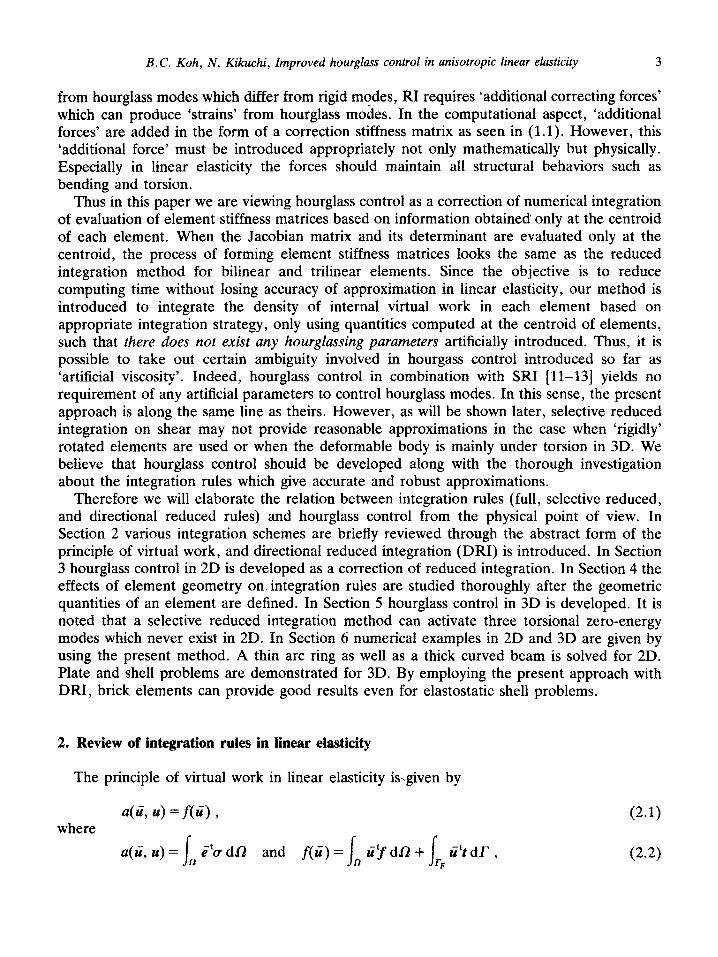
from hourglass modes which differ from rigid modes, RI requires ‘additional correcting forces’ which can produce ‘strains’ from hourglass modes. In the computational aspect, ‘additional forces’ are added in the form of a correction stiffness matrix as seen in (1.1). However, this ‘additional force’ must be introduced appropriately not only mathematically but physically. Especially in linear elasticity the forces should maintain all structural behaviors such as bending and torsion.
Thus in this paper we are viewing hourglass control as a correction of numerical integration of evaluation of element stiffness matrices based on information obtained only at the centroid of each element. When the Jacobian matrix and its determinant are evaluated only at the centroid, the process of forming element stiffness matrices looks the same as the reduced inte~ation method for bilinear and trilinear elements. Since the objective is to reduce computing time without losing accuracy of approximation in linear elasticity, our method is introduced to integrate the density of internal virtual work in each element based on appropriate integration strategy, only using quantities computed at the centroid of elements, such that there does not exist any hourglassing parameters artificially introduced. Thus, it is possible to take out certain ambiguity involved in hourgass control introduced so far as ‘artificial viscosity’. Indeed, hourglass control in combination with SRI [ll-131 yields no requirement of any artificial parameters to control hourglass modes. In this sense, the present approach is along the same line as theirs. However, as will be shown later, selective reduced integration on shear may not provide reasonable approximations in the case when ‘rigidly’ rotated elements are used or when the deformable body is mainly under torsion in 3D. We believe that hourglass control should be developed along with the thorough investigation about the integration rules which give accurate and robust approximations.
Therefore we will elaborate the relation between integration rules (full, selective reduced, and directional reduced rules) and hourglass control from the physical point of view. In Section 2 various integration schemes are briefly reviewed through the abstract form of the principle of virtual work, and directional reduced integration (DRI) is introduced. In Section 3 hourglass control in 2D is developed as a correction of reduced integration. In Section 4 the effects of element geometry on. integration rules are studied thoroughly after the geometric quantities of an element are defined. In Section 5 hourglass control in 3D is developed. It is noted that a selective reduced integration method can activate three torsional zero-energy modes which never exist in 2D. In Section 6 numerical examples in 2D and 3D are given by using the present method. A thin arc ring as well as a thick curved beam is solved for 2D. Plate and shell problems are demonstrated for 3D. By employing the present approach with DRI, brick elements can provide good results even for elastostatic shell problems,
2. Review of integration rules in linear elasticity
The principle of virtual work in linear elasticity isgiven by
46 u) =.m , where
&i, 26) =
4 B.C. Koh, N. K~k~~h~~ Improved hourglass control in ~n~~tro~i~ linear el~t~c~t~
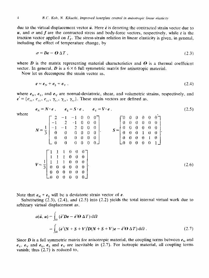
due to the virtual displacement vector U. Here Gis denoting the contracted strain vector due to U, and u and f are the contracted stress and body-force vectors, respectively, while t is the traction vector applied on r,. The stress-strain relation in linear elasticity is given, in general, including the effect of temperature change, by
a=De-OAT, (2.3)
where D is the matrix representing material characteristics and 8 is a thermal coefficient vector. In general, D is a 6 X 6 full symmetric matrix for anisotropic material.
Now let us decompose the strain vector as,
e = eh; + e, + e, , (2.4)
where eN, e,, and e, are normal-deviatoric, shear, and volumetric strains, respectively, and et= {e,v,x, evv, e,,, r,, , ‘Y,,~, r,,.}. These strain vectors are defined as,
e,=N=e, e,=S*e, e,=V*e, (2.5) where
r 2 -1 -I 0 0 0 -1
;
2 -10 u 0
+; -(: -:, 2 0 0 0 0 0 0 0
0 0 0 0 0 0 0 0 0 0 0 0
111000 1 1 1 0 0 0
1 1 1 I 0 0 0 v=s
_ ;
0 0 0 0 0 0 * 0 0 0 0 0 0 000000
1~ s=oooloo 0 0 0 0 0 0 0 0 0 0 0 0 0 0 0 0 0 0 0 1 0 0 0’ 0 ~ 0 0 0 0 0 l_
(2.6)
Note that eN + e, will be a deviatoric strain vector of e. Substituting (2.3), (2.4), and (2.5) into (2.2) yields the total internal virtual work due to
arbitrary virtual displacement as.
(Z”(N + S + V)tD(N + S + V)e - &I AT) d&! . (2.71
Since D is a full symmetric matrix for anisotropic material, the coupling terms between eN and e,, e, and es, e, and ev are inevitable in (2.7). For isotropic material, all coupling terms vanish; thus (2.7) is reduced to,
B.C. Koh, N. Kikuchi, Improved hourglass control in anisotropic linear elasticity
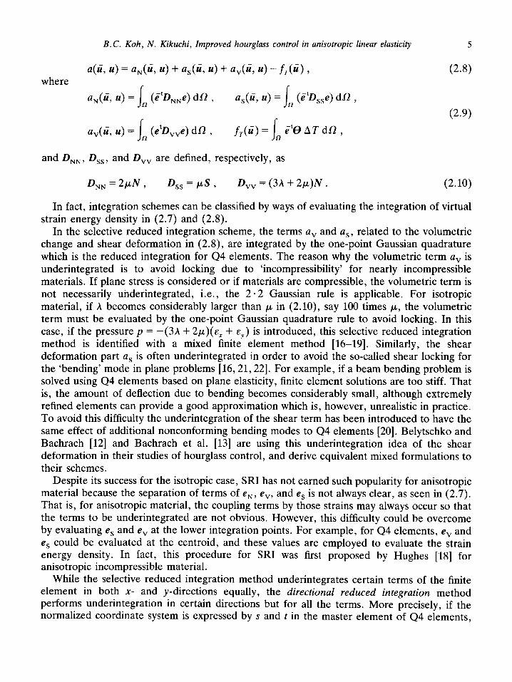
a(li, u) = a,(zi, u) + a&i, u) + u&i, u) -f&i) )
where
u,(ii, u) = R (e’D,,e) da , s
f&-Q = I R &ATdR,
and DNN, Dss, and 4, are defined, respectively, as
D NN=~PN, D,, = /LS, Dvv = (3A + 2j~)N. (2.10)
5
(2.8)
(2.9
In fact, integration schemes can be classified by ways of evaluating the integration of virtual strain energy density in (2.7) and (2.8).
In the selective reduced integration scheme, the terms a, and a,, related to the volumetric change and shear deformation in (2.8), are integrated by the one-point Gaussian quadrature which is the reduced integration for Q4 elements. The reason why the volumetric term a, is underintegrated is to avoid locking due to ‘incompressibility’ for nearly incompressible materials. If plane stress is considered or if materials are compressible, the volumetric term is not necessarily uhderintegrated, i.e., the 2 - 2 Gaussian rule is applicable. For isotropic material, if A becomes considerably larger than Al. in (2.10), say 100 times p, the volumetric term must be evaluated by the one-point Gaussian quadrature rule to avoid locking. In this case, if the pressure p = -(3A + ~F)(E, + eY) is introduced, this selective reduced integration method is identified with a mixed finite element method [16-191. Similarly, the shear deformation part a, is often underintegrated in order to avoid the so-called shear locking for the ‘bending’ mode in plane problems [16,21,22]. For example, if a beam bending problem is solved using Q4 elements based on plane elasticity, finite element solutions are too stiff. That is, the amount of deflection due to bending becomes considerably small, although extremely refined elements can provide a good approximation which is, however, unrealistic in practice. To avoid this difficulty the underintegration of the shear term has been introduced to have the same effect of additional nonconforming bending modes to Q4 elements [20]. Belytschko and Bachrach [12] and Bachrach et al. [13] are using this underintegration idea of the shear deformation in their studies of hourglass control, and derive equivalent mixed formulations to their schemes.
Despite its success for the isotropic case, SRI has not earned such popularity for anisotropic material because the separation of terms of eN, e,, and e, is not always clear, as seen in (2.7). That is, for anisotropic material, the coupling terms by those strains may always occur so that the terms to be underintegrated are not obvious. However, this difficulty could be overcome by evaluating es and ev at the lower integration points. For example, for Q4 elements, e, and e, could be evaluated at the centroid, and these values are employed to evaluate the strain energy density. In fact, this procedure for SRI was first proposed by Hughes [18] for anisotropic incompressible material.
While the selective reduced integration method underintegrates certain terms of the finite element in both X- and y-directions equally, the directional reduced integration method performs underintegration in certain directions but for all the terms. More precisely, if the normalized coordinate system is expressed by s and t in the master element of Q4 elements,

6 B.C. Koh, N. Kikuchi, Improved hourglass control in anisotropic linear elasticity
underintegration is applied only in either s- or t-direction. For three-dimensional problems three directions Y, s, and t exist in the master element. Thus, underintegration would be applied in the Y/S/t-direction.
Why must the direction reduced integration method be introduced? A reason for this is the unsatisfactory response of the selective reduced integration method for the shear locking which has been pointed out by several authors [21,22,24]. Suppose that a slender rectangular Q4 element is inclined in the x-y physical global coordinate system as shown in Fig. 1. If a bending moment is applied, the shear deformation ysy,, should not contribute large amounts of internal virtual work for a very slender ‘beam’. This physical consideration implies negligible effect of ‘y,, but not of yIy. In other words, if the selective reduced integration method is applied blindly to the shear term ‘y,,, then it is impossible to reflect physical reality. Indeed, since +y,, is written by
Yst = k - eY,) sin 28 + ‘yXY cos 28 , (2.11)
where 13 is the angle of the ‘beam’ axis to the x-axis, the one-point underintegration must be applied to the terms related to ys,. This means that the reduced integration must be applied to the combined term of eXX, eyy and yXy,,. If the selective reduced integration method is applied
for Y,,, this yields physically nonsense underintegration in order to avoid the shear locking. If the bending is along either the X- or y-axis, underintegration of xv is fine. Otherwise, this scheme yields considerable error. That is, if the hourglass control scheme introduced by Belytschko and Liu is applied without further consideration, results may suffer by this deficiency of the selective reduced integration method. The directional reduced integration method is, thus, introduced to correct this difficulty. However, it is noted that the directions s and t must be set up appropriately to reflect exact physics. In general, this is a very difficult task because the solution is unknown a priori. In other words, it is very difficult to set up the axis s and t so that underintegration is correctly applied. Nonetheless this approach is still attractive since such reduced integration is necessary for the shell, plate, and beam structures whose principal axes are a priori known from their geometry. For such ‘thin’ structures most finite elements have very large aspect ratios among the representative element lengths h,, h,, . and h, in each direction corresponding to the normalized axes r, s, and t, respectively. If the t-direction is almost the same as the thickness direction of this shell structures, the aspect ratios h,lh, and h,Tlh, are, in general, very large. In this case, reduced integration would be
Fig. 1. The rotation of the coordinate system.

B.C. Koh, N. Kikuchi, Improved hourglass control in anisotropic linear elasticity
Table 1 Integration rules and quadrature points
a,(6 u) a,@, 4 a,(& 4 Remarks
FI 2*2 2*2 2*2 a, can be evaluated at SRI 2*2 l*l l*l 2 * 2 points for SRI and DRI DRI 2*1/1*2 1*2/2*1 l*l for compressible material RI l*l l*l l*l
applied in the r- and s-directions, that is, reduced integration is introduced in the direction which has much larger geometric size. If a slender beam is discretized with &node brick elements and if the r-direction coincides with the beam axis, the aspect ratios h,lh, and h,lh, of elements usually become large. In this case, reduced integration might be applied only in the r-direction. For a fat or thick structure, aspect ratios h,lh,, h,lh,, and h,lh, are, in general, almost unit. For such elements reduced integration may not be applied since the existence of shear locking is not likely. Thus, if ‘reasonable’ finite element gridding is expected, direction reduced integration can be controlled solely by the aspect ratios between h,lh,lh,.
Table 1 shows the Gaussian quadratures to integrate (2.8) following the related integration scheme with Q4 isoparametric elements for plane problems. All numbers indicate the number of integration points in each direction of the natural coordinates.
3. Hourglass control in two dimensions
Let us consider a Q4 element for plane elasticity problems whose shape functions are given
bY
N&J)= i(l+SpS)(l+tJ), (Y’l,. . . ,4, (3-l)
in the normalized coordinate system (s, t). Here (S (I, t, ) are normalized coordinates of four corner nodes of the square master element whose side length is 2 as shown in Fig. 2(a).
Applying isoparametric approximations for the geometry and displacement components, we have A t Y 3
4 1 3 4
-1
1
,s ~ 1
1 -1 2 2
x
(a) (b) Fig. 2. Q4 elements in 2D. (a) The normalized coordinate system. (b) The physical coordinate system.
B.C. Koh. N. Kikuchi, Improved hourglass control in anisotropic linear elasticity
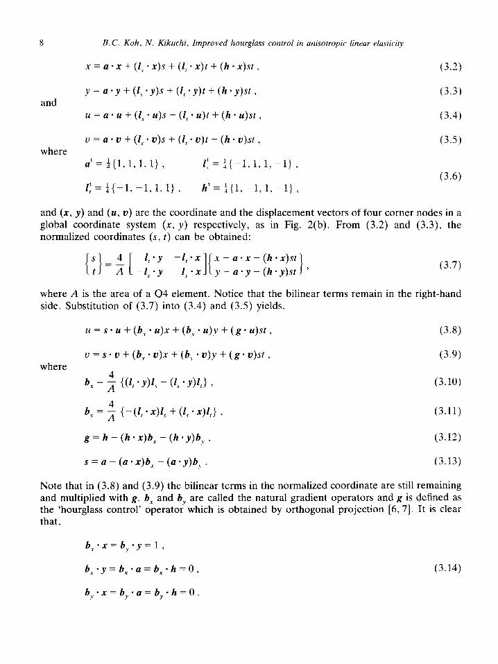
x = a * x + (1, * x)s + (I, * x)t + (h - x)st , (3.2)
and y=u-y+(z;y) s + (I, *y)t + (h .y)st , (3.3)
u = a * u + (z,s - 24)s + (I, - up + (h - u)st , (3.4)
u = a - u + (I,, * u)s + (I, - v)t + (h * u)st , (3.5) where
a’ = i{l, 1, 1, l} , 1: = ${-I, l,l, -l} ,
(3.6) z: = ${-1, -l,l, l} ( h’= +{l, -1,l. -l} ,
and (x, y) and (u, u) are the coordinate and the displacement vectors of four corner nodes in a global coordinate system (x, y) respectively, as in Fig. 2(b). From (3.2) and (3.3)) the normalized coordinates (s, t) can be obtained:
x--a-x-(h.x)st
y-u.y-(h.y)st (3.7)
where A is the area of a Q4 element. Notice that the bilinear terms remain in the right-hand side. Substitution of (3.7) into (3.4) and (3.5) yields,
u=s.u+(b,.u)x+(b;u)y+(g.u)st, (3.8)
u=s~u+(b,~u)x+(b?,w)y+(g~u)st, (3.9) where
b, = ; HZ, .Y)l, - (I., . Y)U 3 (3.10)
b, = f {-(I, * x)Z, + (1, * x)Z,} ) (3.11)
g=h-(h*x)b,-(h*y)b,, (3.12)
s=u-(u~x)b,-(u*y)b,.. (3.13)
Note that in (3.8) and (3.9) the bilinear terms in the normalized coordinate are still remaining and multiplied with g. b, and b, are called the natural gradient operators and g is defined as the ‘hourglass control’ operator which is obtained by orthogonal projection [6,7]. It is clear that,
b;x=b;y=l,
(3.14)
b;x=b,w=b;h=O.

B.C. Koh, N. Kikuchi, Improved hourglass control in anisotropic linear elasticity 9
Notice that (3.8) and (3.9) are obtained by simply inverting the transformation equation (3.7); therefore, in the same way the hourglass control procedure can be easily extended to evaluate any terms which involve the bilinear terms of st. These equations are also developed by Belytschko and Bachrach [12] employing the orthogonality conditions (3.14).
Indeed, the first derivatives with respect to x and y can be written in terms of s and t as follows:
(3.15)
where J is the coordinate transformation matrix defined as
J=[:‘~ “;2]=[ Z;x+(h*x)t Z;y+(h*y)t
Z;x+(h*x)s I E;y+(h*y)s ’ (3.16)
and 21 22
J = JA - Jr,.!,, = Jo + 1,s -t J2t, (3.17)
J0 = (l/x)(l;y) - (Z;y)(l;x) = A/4, (3.18)
J1 = (I, * x)(h * y) - (Z, * y)@ l x) , (3.19)
J2 = (Z;y)(h*x) - (Z;x)(h*y). (3.20)
Note that for a rectangular or a parallelogram element, J = Jo and J1 = J2 = 0 since h m x = hay = 0 (see Table 3).
By using (3.8) and (3.9), (3.15) and (3.16), the strain vector can be written as
where (3.21)
(3.22)

10 B.C. Koh, N. Kikuchi, improved hourglass control in anisotropic linear elasticity
In (3.21) e, is a constant strain vector and the last two terms are denoting the ‘directional’ variations of e in an element with respect to the normalized coordinate. Equations (3.22) can be rewritten as,
e, = B,d , e,$ = B,d , e, = B,d , (3.23)
where d is the nodal displacement vector defined by,
(3.24)
B,, B,, and B, are the constant, s-, and t-directional parts of an element gradient matrix, and
b 0 b,, 0 h,, 0 b,, 0 B, = 0”’ b,, 0 $2 0 b,, 0 $4 ,
b j-1 bx, by, k2 by3 bx, $4 k‘i 1 i
%l 0 cg2 0 cg, 0 cg4 0
B, = 0 q, 0 a& 0 a87 0 ag4 ,
ag1 %I ag2 cg2 ath cg3 ag4 cg4 1 0 4, 0 &, 0 4h 0 0 bg, 0 bg, 0 bg, ,
dg, bg, dg, bg, dg, bg, dg, 1 (3.25)
where ra=l;x, b=-Z,*x, c=-Z,*y, d=Z;y, and b,;, byj, gi (i=1,...,4) are the components of b,, b,, and g.
If the strain vector e is evaluated at the centroid, then e = e, since s = t = 0. Since the reduced integration scheme (RI) evaluates an element stiffness matrix only at the centroid, (3.21) represents all strains by RI. Due to the orthogonality conditions (3.14). all strains of (3.21) vanish everywhere in an element if and only if
u = C,p - Gy + C,h , u = C,a + C,x f C,h ,
where C, - C, are arbitrary constants. This means that five deformation modes induce zero strain when RI is employed. Physically there exist only three rigid displacement nodal vectors in two dimensions, such as (a’, 0’}, (0: a’}, and {-y’, x’} which don’t induce strain (thus, strain energy). However for RI, {h’, 0’) and (0: h’} also appear as zero energy displacements, while both modes represent bending modes in two dimensions as in Fig. 3. Numerically, this
(a) (b) Fig. 3. Two bending hourglass modes in 2D.
B.C. Koh, N. Kikuchi, Improved hourglass control in anisotropic linear elasticity 11
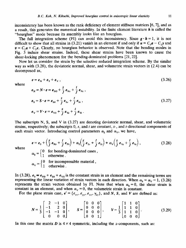
inconsistency has been known as the rank deficiency of element stiffness matrices [6,7], and as a result, this generates the numerical instability. In the finite element literature h is called the “hourglass” mode because its assembly looks like an hourglass.
The full integration scheme (FI) can avoid this inconsistency. Since g l h = 1, it is not difficult to show that all strains in (3.21) vanish in an element if and only if u = C,,a - C,y and u = C,a + C,x. Clearly, no hourglass behavior is observed. Note that the bending modes in Fig. 3 induce shear strains. Indeed, these shear strains have been known to cause the shear-locking phenomenon for the bending-dominated problems [21,22].
Now let us consider the strain by the selective reduced integration scheme. By the similar way as with (3.28), the deviatoric normal, shear, and volumetric strain vectors in (2.4) can be decomposed as,
where e = eN + es + e, , (3.26)
e, = S l e = es, + s es, + 4 e J J St,
e, = V- e = e,, + s. J 5% + f evt *
(3.27)
The subscripts N, S, and V in (3.27) are denoting deviatoric normal, shear, and volumetric strains, respectively; the subscripts 0, s, and t are constant, s-, and t-directional components of each strain vector. Introducing control parameters (Ye and (Y,,, we have,
s e=e,+ j % :e
J vs (3.28) where
for bending-dominated cases ,
0 av =
for incompressible material , 1 otherwise .
In (3.28), e, = eNO + es, + e,, is the constant strain in an element and the remaining terms are representing the linear variation of strain vectors in each direction. When (us = q, = 1, (3.28) represents the strain vectors obtained by FI. Note that when cys = 0, the shear strain is constant in an element, and when (Y,, = 0, the volumetric strain is constant.
For the plane strain case, e’ = {eXX, ey,, , err, y,,}, and N, S, and V are defined as:
(3.29)
In this case the matrix D is 4 x 4 symmetric, including the z-components, such as:
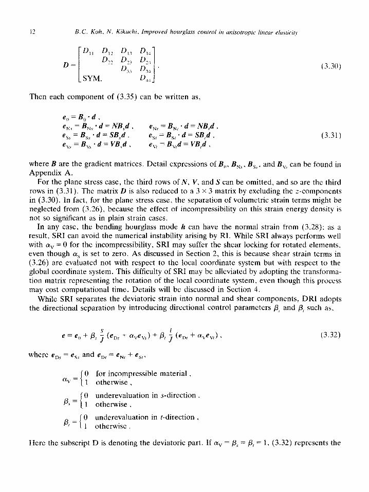
12 B.C. Koh. N. Kikuchi, Improved hourglass conml in unisotropic linear elasticity
(3.30)
Then each component of (3.35) can be written as.
e,, = B,, ‘ d . eNs = B,, * d = NB,d , e,,s = Bsc l d = SB,yd .
ev,s = &, - d = VB,d ,
where B are the gradient matrices, Appendix A.
eNr = B,, - d = NB,d , e,, = B,, - d = SB,d ,
ev, = B,d = Vl3,d ,
(3.31)
Detail expressions of B,,, B,, . B, , and B, can be found in
For the plane stress case, the third rows of N, V, and S can be omitted, and so are the third rows in (3.31). The matrix D is also reduced to a 3 X 3 matrix by excluding the z-components in (3.30). In fact, for the plane stress case, the separation of volumetric strain terms might be neglected from (3.26), because the effect of incompressibility on this strain energy density is not so significant as in plain strain cases.
In any case, the bending hourglass mode h can have the normal strain from (3.28); as a result, SRI can avoid the numerical instability arising by RI. While SRI always performs well with (TV = 0 for the incompressibility, SRI may suffer the shear locking for rotated elements, even though cys is set to zero. As discussed in Section 2, this is because shear strain terms in (3.26) are evaluated not with respect to the local coordinate system but with respect to the global coordinate system. This difficulty of SRI may be alleviated by adopting the transforma- tion matrix representing the rotation of the local coordinate system, even though this process may cost computational time. Details will be discussed in Section 4.
While SRI separates the deviatoric strain into normal and shear components, DRI adopts the directional separation by introducing directional control parameters p, and p, such as,
e = 6 + P, 5 (en, +
where e,, = es, and en, = eNr
avevs > + P, -j (en, + avev,) .
+ es,,
(3.32)
10 for incomoressible material , a, = I 1 otherwise’,
8.5 = { 0 underevaluation in s-direction ,
1 otherwise ,
P, =( 0 underevaluation in t-direction ,
1 otherwise .
Here the subscript D is denoting the deviatoric part. If LG., = fi, = p, = 1, (3.32) represents the

B.C. Koh, N. Kikuchi, Improved hourglass control in anisotropic linear elasticity 13
same strain vector obtained by FI. If p, = p, = 0, (3.32) depicts constant strain in an element. Note that in (3.32) no separation between normal and shear strains is performed.
Each component of (3.40) can be expressed as:
e, = B, - d ,
e,, = B,, - d , eDt = BDt ’ d , (3.33)
where B,, = B,, + B,, and B,, = B,, + B,,. All Bs are defined by the same as in (3.31). Explicit expressions of Bs are given in Appendix A. Indeed, it is easy to show that bending hourglass modes can have strains from (3.33). When czv = 0, DRI can eliminate the locking for incompressible material and by properly setting /?, or p, = 0, DRI can also eliminate the shear locking. In addition, DRI can avoid the difficulty of SRI due to element rotation. In fact, this difficulty of SRI is caused by employing different integration rules to strain components in the numerical sense; thus, this can be avoided by employing the same integration to all components, which is the way DRI exactly follows. Let us here briefly review how DRI evaluates strains, assuming that an element is slender and rectangular where h, S- h,. Here h, and h, denote the lengths of sides in the s- and t-direction in Fig. 1. In this case p, = 0 or p, = 1. Since b = c = 0 for a rectangular element, (3.33) reduces to
t e = e, + - e, ,
J (3.34)
where e, = B, * d ,
B,= 0 0 0 0 0 0 0 0 .
[
d& 0 d& 0 d& 0 d& 0
0 d& 0 d& 0 d& 0 da 1 If (h’, 0’) is a more dominating bending mode than (O’, ht), then d =
C{l, 0, -1, 0, 1, 0, -1, 0}, where C is an arbitrary constant. This is often true for the element discussed now. Then the shear strain in e, can be eliminated so that the shear locking can be avoided.
3.1. Evaluation of strain energy density
Now let us evaluate the strain energy density in an element with strains obtained in (3.21), (3.28), or (3.32). Then,
(3.35)

14 B.C. Koh, N. Kikuchi. Improved hourglass control in anisotropic linear elasticity
Here the relations In, s/J dR = Jn t/J da = 0 have been applied. Using the relation of strain-displacement (3.23), we obtain:
where
st (BjDB, + BjDB,) dfl)d , J” (3.36) e
B, = B,, + +Qs + avBv, , B, = B,, + aSBSI + avB, . (3.37)
Here (Ye, q, are the strain control parameters and p,, p, are the directional control parameters; thus by putting proper values for the parameters, we can employ certain design integration schemes following FI, SRI, or DRI. Noting that the first term on the right-hand side in (3.37) has the same expression of strain energy density by RI, we can consider the remaining terms as the correction terms to the evaluation by RI. Suppose that,
Cl1 = e GdQ=.f $ J +J,'+Jt )
a1 0 1 a 2a
Cl2 = I
S’dO=O, % J2
(3.38)
(3.39)
where (s,, t,), a = 1, . . . ,4, are the coordinates of integration points in the normalized coordinate system. When an element is rectangular, cl1 = 2 and c,~ = 0 because J, = J2 = 0.
Finally, we have,
I “e F’De da = d’(B#B,)A + c11/3,B;DB, + cll&B:DB, , (3.40)
where B, and B, are defined the same as in (3.25). Table 2 shows the relationship between control parameters (Y, p and the corresponding integration rules. If p, = p, = 1 and (Y = (Y~ = (TV we can have similar correction terms of hourglass control with an “artificial stiffness” parameter [6].
Table 2 Control numbers and integration rules
P* P, Integration rule
1 1 1 0” Ob 1 1 1 l/O
1 FI (full) 1 SRI (selective reduced)
l/O DRI (directional reduced)
a For bending-dominated case. b For nearly incompressible material.
B.C. Koh, N. Kikuchi, Improved hourglass control in anisotropic linear elasticity 15
3.2. Extension of hourglass control
Now let us evaluate the virtual works due to temperature change and body force. Indeed, this attempt may generalize hourglass control as a computing tool which can reduce the computing time while the previously introduced hourglass control has been developed only for the stabilization method.
Suppose that the ‘temperature’ AT is given by
AT= f: AT,N,(s,t)=a.A\T+s(Z;AT)+t(f;AT)+st(h*AT), (3.41) a=1
where AT is a nodal vector of temperature change, and a, l,, I,, and h are defined the same as in (3.6). The internal virtual work by the temperature change in (2.7) is given by, because of (3.21) and (3.23),
= d’(AT,B:, + p, AT,,B; + p, AT,,B:)e , (3.42) where
AT, = I .n,
AT da = +(AT, + ATE + ATE + AT,)A, ,
AT,, = e
5 AT da = $(-AT, + AT, + ATE - AT,), (3.43)
AT,, = I n ;ATdn=j(-AT,-AT,+AT,+AT,),
e
and B,, B,, and B, are defined the same as in (3.25). Notice that the directional control parameters p,, p, are used in (3.42).
Let us assume that the body force in (2.2) is also linearly distributed in an element. Then the similar expression to (3.5) and (3.6) of the displacements is available for the body force vector. That is,
where f, and fY are the nodal component vectors of the body force. Then the work done by the body force can be written as,
(3.45)
(3.46)

16 B.C. Koh, N. Kikuchi. Improved hourglass control in anisotropic
Detailed expressions for M,,, M,, and M2 are given in Appendix B.
linear elasticity
If p,V = j3, = 1, we obtain:
r4 2 1 2
. M, = ;
0 0 1 ’
2 I
: -2 -1 021 012 0 0 (1 0 -2 -1 0 0
(3.47)
Note that the mass matrix M in (3.46) consists of the Jacobian components J,,, J, , and J, which are representing the distortion of an element. For an undistorted element (e.g. a rectangle or a parallelogram), 1, = JZ = 0 so that the mass matrix M = J,,M,, = i ACM,,, where A, is the area of an element.
4. The effects of the element geometry on the integration rules
Before extending the hourglass control to 3D, let us consider the effects of an element geometry on the integration rules. This study is worthwhile since finite element solutions are strongly dependent upon the geometry of an element. The geometry of an element can be represented by Jacobian matrix (3.16) and its determinant (3.17). Using these quantities, the quality of integration rules can be easily investigated based on (3.30)-(3.35) for the fundamental deformation modes obtained by the eigenvalue analysis of an element.
4.1. Preliminary
Q4 elements can be divided into three groups, as shown in Fig. 4, according to their shapes. Since the geometry transformation between the master element and any Q4 element is
obtained by Jacobian matrix J their components can be considered as the shape indicators representing the rotation and distortion of an element. decomposed as:
J= J*R where J* = g and R= g,
and s, x, X are a normalized, local (unrotated), and global (rotated) coordinate system,
Indeed, any Jacobian matrix can be
(4.1)
(‘3) (b) CC)
Fig. 4. Shapes of Q4 elements. (a) Rectangles. (b) Parallelograms. (c) Arbitrary shapes.
B.C. Koh, N. Kikuchi, Improved hourglass control in anisotropic linear elasticity 17
Table 3 Element shapes and the geometry quantities in J”
Rectangle Parallelogram Arbitrary Q4
J* 1, * x
4 ‘Y
J* = J;
not zero
J* = J;
not zero
J* # J,*
not zero
1, ‘X
1, ‘Y
0 0
not zero not zero
hex 0
hey 0
a J* is defined as:
0
0 not zero
1,-x+ h-x 1,-x+ h-x 1 l;y+h-y . respectively. Since R, which represents the rigid rotation of the coordinate system, doesn’t change the shape of an element, J* can be considered as the matrix quantifying pure element distortion.
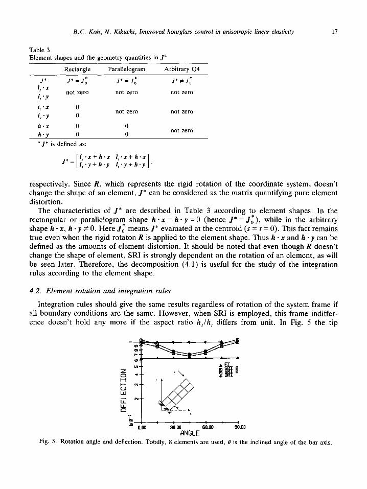
The characteristics of J* are described in Table 3 according to element shapes. In the rectangular or parallelogram shape h - x = h - y = 0 (hence J* = J,*), while in the arbitrary shape h l x, h * y # 0. Here Jo* means J* evaluated at the centroid (s = t = 0). This fact remains true even when the rigid rotaton R is applied to the element shape. Thus h - x and h - y can be defined as the amounts of element distortion. It should be noted that even though R doesn’t change the shape of element, SRI is strongly dependent on the rotation of an element, as will be seen later. Therefore, the decomposition (4.1) is useful for the study of the integration rules according to the element shape.
4.2. Element rotation and integration rules
Integration rules should give the same results regardless of rotation of the system frame if all boundary conditions are the same. However, when SRI is employed, this frame indiffer- ence doesn’t hold any more if the aspect ratio h,lh, differs from unit. In Fig. 5 the tip
Fig. 5. Rotation angle and deflection. Totally, 8 elements are used, 0 is the inclined angle of the bar axis.

18 B.C. Koh, N. Kikuchi, Improved hourglass control in anisotropic linear elasticity
Table 4 Deflections of a beam with respect to the aspect ratio and the rotation angle; NELX is the total number of elements, h, and h, are the lengths of the sides of the elements
Rotation
h,‘h, angle SRI A DRI NOBI” NELX
1 0” 0.99321 0.99493 0.99320
4.5” 0.99321 0.99493 1.1438 20
2 0 0.98107 0.98792 0.98099
45” 0.77837 0.98792 0.92675 10
2.5 0 0.97298 0.98292 0.97308
45” 0.66421 0.98292 0.81095 8
10 0 0.91592 0.93977 0.91596 45” 0.30522 0.93977 0.40118 4
a Is evaluated by following Liu et al. [lo].
defletions of a beam are shown with respect to the rotation angle of the frame of the system. Here 8 rectangular elements are used for the discretization.
SRI, developed to avoid the shear locking, gives stiffer results as the rotation angle increases up to 45” (in Fig. 5, more than 30% than in the unrotated case), while FI and DRI give the same result. At 45”, the result by SRI is the worst and, indeed, almost same as the one by FI. After 45”, SRI recovers its accuracy symmetrically along the line of 45”. This
8, ,“s
B I? ti h=” 8.. . ps CONTROL UHILE P 1 -1
l- (II pt CONTROL WILE p, -1
Lo 1 i 0.25
CCINTOLD.~“MBER “$ 1.00
Fig. 7. Deflection with respect to the directional control numbers.

B.C. Koh, N. Kikuchi, Improved hourglass control in anisotropic linear elasticiry 19
observation could be explained with (2.1). If shear strain is underevaluated in the global coordinates, then yXY = 0, and ‘y,, = (E,, - cYY) sin 28. Thus, at 45”, yTYst will be the maximum and will be distributed symmetrically about 45”.
The violation of the frame indifference by SRI depends on the element aspect ratio. Table 4 and Fig. 6 show the tip deflections of an unrotated and a 45”-rotated beam with respect to the aspect ratios h,/h,. Here, h, and h, denote the side lengths of elements in the axial and the thickness direction, respectively. Only for square elements (i.e. h,/h, = 1.0) SRI provides consistent results in both rotated and unrotated cases. However, as h,lh, is increased, SRI gives gradually stiffer solutions when the elements are rotated.
The difficulty of SRI, arising due to the rotaton of the frame, can be overcome by introducing the decomposition of J as in (4.1). That is, first construct element stiffness matrices by using J* of the local coordinate system, and then multiply R to the local stiffness matrices by recovering the element rotation. However, this manipulation seems awkward because it increases the amount of computation significantly. Therefore, it would be better to search for another integration rule. Bachrach et al. [lo] developed the “directional” or- thogonalization technique in combination with SRI, but this technique can’t remove it, as seen in Table 4.
REMARK 4.1. The difficulty of SRI for element rotation is caused by applying different integration schemes to the terms of shear and normal strains, both of which are related to the shear modulus. If only the stability were not concerned, the di~culty for element rotation can be avoided in numerical sense, by segregating all terms related to the shear modulus and by applying the same integration rule to these terms.
Figure 7 shows the tip defections of a beam with respect to directional control numbers p,,
Fig. 8. The distortion sensitivity of integration rules with 8 elements.
Max (h-x/l l x ) occl_lrs at the star&d elements
20 B.C. Koh. N. Kikuchi. Improved hourglass control in anisotropic lirlear elasticit?
& which are defined as in Section 3. Here the s- and t-direction coincide with axial and thickness directions of the beam, respectively, and 8 rectangular elements are used. p,V = p, = 1 resumes the full integration rule. When p,, = 0 and p, = 1. an almost exact solution is obtained; however, as p, increase the solution deteriorates drastically. When /3, = 1 and p, is varied, the results are not much different. In other words, approximated solutions are strongly dependent on p,, which is the control number in the axial direction.
Therefore, in this case the directional reduced integration of p, = 0 and p, = 1 can be used as a substitute of SRI. Since DRI employs the same integration rule for all the terms of shear modulus, the ‘frame indifference’ on element rotation can be achieved regardless of the aspect ratio of elements, as observed in Fig. 5 and Table 4. Since two directional controls are possible for a Q4 element, such as 1 .2 or 2. 1. the direction to be controlled is not easy to be determined a priori. This direction may be chosen by the ratio of the sides of element such that the direction of the longer side would be underintegrated.
4.3. Element distortion and integration rules
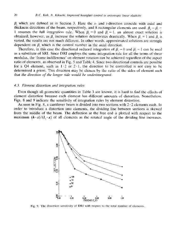
Even though all geometric quantities in Table 3 are known, it is hard to find the effects of element distortion because each element has different amounts of distortion. Nonetheless. Figs. 8 and 9 indicate the sensitivity of integration rules by element distortion.
As seen in Fig. 8, a cantilever beam is divided into two sections with 2.2 elements each. In order to introduce a distortion into elements, the dividing line between sections is skewed from the middle of the beam. The deflection at the free end is plotted with respect to the maximum (h - x)l(Z, - x) of all elements as the rotated angle of the dividing line increases.
?. 0.20 0.40 0.60 0.80 1.00
tiRX(HX/LX)
Fig. 9. The distortion sensitivity of DRI with respect to the total number of elements.

B.C. Koh, N. Kikuchi, Improved hourglass control in anisotropic linear elasticity 21
Since k- - x and h *_y defined the amount of distortion and Z, - x and I, - y are only nonzero values for an unrotated rectangular element, h l x/l, - x and h l y/Z, * y can be defined as nondimen- sionalized indicators of element distortion. With these discretizations, Z, - y = h - y = 0 and thus h - x/Z, - x = J,lJ,, where J, and J, are defined in (3.23). Generally, DRI gives better soZutions than others, although the approximations deteriorate quickly as h l x/l, - x increases.
In Fig. 9 the distortion sensitivity of DRI is examined as the number of elements increases. When h -x/Z, l x is greater than 0.2, DRI fails to give any reasonable approximation even though a large enough number of elements are used. Therefore, the values of the distortion indicators may be limited to 0.2 in order to assure a good approximation, At the level of finite element gridding, if h * x/Z, - x and h -y/Z, * y become greater than 0.2 in certain finite elements, warning of possible dete~oration of quality of approximation should be provided to users for the application of DRI method.
5. Hourglass control in three dimensions
Even though the hourglas control method in 3D could be developed as the simple extension from 2D, its application in solid mechanics couldn’t be a trivial extension. When the reduced integration scheme is employed for an &node brick element, there appear 12 hourglass modes, including 6 bending-type and 3 torsion-type modes which never occur in 2D. Therefore, these torsion-type hourglass modes could be easily activated even if the hourglass control method, which might be successful in 2D, is employed.
Unfortunately, previous 3D hourglass control methods have been developed only for l-degree field problems (such as the heat conduction problem), and have been taken for granted for solid mechanics without conside~ng any physical situations. Since the advantage of the hourglass control method is more appreciated in 3D, hourglass control in 3D should be examined thoroughly along with the physical problems.
5.1. Derivation of hourglass control in 3D
Consider an &node brick element in the normalized coordinate system (r, s, t) as in Fig. IO, whose side length is 2. Its shape functions are,
N,(r,s,t)=~(l+r,r)(l+s,s)(l+t,t), cx=l,..., 8, (54
where CY is the element node number defined as in Fig. 10. The linear isoparametric approximations for the position and displacement in an element
yield,
8 x= 2 x,N,(r, s, t) = (s - x) f (f, l x)r + (Z2 - x)s + (l, - x)t
a=1
+ (h, l x)st f (h, * x)tr -I- (h, - x)rs f (h, l x)rst , (5.2)

22 B.C. Koh, N. Kikuchi, Improved hourglass control in anisotropic linear elasticity
a) b)
Fig. 10. Numbering of an g-node brick element. (a) Physical coordinates. (b) Master coordinates.
u = 2 u,iv,(r, s, t) = (s - u) + (I, * u)r + (I, - u)s + (1, - u)t a=1
+ (h, * u)st + (h, * u)tr + (h, ’ u)rs + (h, * u)rst ) (5.3)
where x and u are the nodal position and displacement vector in the x-direction, and
St = ${l, l,l, l,l, l,l, l} ,
1; = 3(-l, l,l, -1, -l,l, 1, -l} )
1; = i{-1, -l,l, 1, -1, -l,l, l} )
z; = Q{-1, -1, -1, -l,l, l,l, l} ,
lz; = i{l, 1, -1, -1, -1, -l,l, 1))
h; = i{l, -l,l, -1, -1, l,l, -1) )
h\ = f{l, -l,l, -1, 1, -1, 1, -l} )
hi= Q{-l,l, -l,l, 1, -l,l, -l},
Xt = {x, 9 x2, xg, x4, x5> x(j, x7, x8) * (5.4)
Similar expressions for positions and displacements in the y- and z-directions are possible.
Then the counterpart of (3.7) in 2D is,
[I 1
,’ X - s * X - (h, * x)st - (h, * x)tr - (h, * X)TS - (h, * x)rst
= [Cii] y - s ’ y - (h, * y)st - (h, * y)tr - (h, * y)rs - (h, * y)rst , (5.5) t 2 - s . z - (h, * 2)st - (h, * z)tr - (h, * z)rs - (h, * z)rst
where 1
I, l x Qy
I
. (5.6) I, * z

B.C. Koh, N. Kikuchi, Improved hourglass control in anisotropic linear elasticity
Substituting (5.5) into (5.3), we obtain,
u = g, * u + (b, * U)X + (b, * u)y + (b, l U)Z
+ (g, * u)st + (g, l u)tr + (g, l 11)rs + (g, * u)rst , where
bi = i Ci,l, , i=1,...,3, a=1
23
gi = hi - (hi l x)b, - (hi l y)b, - (hi. z)b3 , 1 = 1, . . . ,4 ,
g, = s - (s*x)b, - (s*y)b, - (s.z)b3 .
Then the following orthogonality holds:
b,*x=b,*y=b,*z=l,
b,*y=b,.z=b,.h,=O ’
b,*x=b,.z=b,*h,=O ’ i=1,...,4. (5.11)
Similar expressions to (5.7) are available for u and W. Note that g, , g,, g,, and g, have the same forms as the hourglass gradient operators in Belytschko [6] except for constants.
Then we obtain the engineering strain vector with the directional components as:
tr e = e, + I e, + s e, + 4 e, + Is ers + 7 e,, + J e,,
J J J J 2
+ 3 e,2 + * * (5.12)
where e’ = { eXX, eY,, , err, y,,, , y,,,, , y,,} , and e is the strain vector evaluated at the centroid and all others are directional components. Notice that (5.12) includes the biquadratic components. However, the decomposition (5.12) of a strain vector is not realistic since this procedure takes too many operations to reduce the computational time, which is a main goal of hourglass control. Thus, in order to overcome this difficulty, it may be reasonable to take some approximation for the strain decomposition (5.12).
If the shape of an 8-node brick element is almost parallelopiped, then hi l x = hi l y = hi * z = 0, where i = 1, . . . , 4. In this case the Jacobian matrix J and its determinant J can be approximated as:
J=C’ and J=J,=C,,, (5.13)
where C is defined as in (5.6), and the subscript 0 denotes the value at the centroid. From (5.13), (5.12) reduces to,

24 B.C. Koh, N. Kikuchi, Improved hourglass control in anisotropic linear elasticity
e = e,, + p, f e, f P, f e,v + P, + e, 0 II 0
+ P,P, f e,<, + P,P, F e,, + PA 7 ers . 0 0 0
(5.14)
where p,, p,, and p, are the directional control parameters. A similar decomposition of the strain to (5.14) can be found in Liu et al. [6,25], after setting all j3s equal to 1. As we did in 2D, each directional component can be decomposed into the deviatoric-normal, shear. and volumetric strains with strain control parameters (Y~ and cyv. Since our main interest lies on directional integration, such strain decomposition regarding to SRI is not given. However. the characteristics of hourglass control with SRI will be discussed later in this section.
Each strain components of (5.14) can be written explicitly as:
e, = B,, * d ,
e, = B, - d , e,y = B, - d , e, = B, * d , (5.15)
e st = B,T, - d , err = B,, * d . err = B,,? * d ,
where d’ = {IA,, u,, wI, . . . , u3, u3, w3} is a nodal displacement vector and all Bs are 6 + 24 gradient matrices. Details of B are given in Appendix C. Then the internal virtual work can be written as:
+ P, P, $ JoB,s,Wu + P, P, 8 JoBPL +‘P, P,y % JAPL )d 3 (5.16)
where V is the volume of an element. Indeed, the evaluation of (5.16) is quite tedious. However, its reduction of computation
time is considerable compared to FI, because the computation for constructing element stiffness matrices includes the evaluation of the Jacobian matrix, its inverse, and others as well as (5.16). Table 5 shows the CPU time to construct an element stiffness matrix for isotropic material by Amdahl 5860 and Apollo DN560. Here the beam bending problem of Fig. 14 is solved, where all elements are quite regular; thus (5.16) becomes an exact expression for this case since hi - x = h, - y = hi - z = 0, i = 1, . . . , 4. The explicit algorithm by hourglass control provides an almost 4-5 times faster comptation than that by FT.
Table 5 The CPU time to construct an SKE for a parallelopiped element in Fig. 12
Method Apollo 560 Amdahl Deflection
FI 2.3378 us 0.100 0.8329 DRI 0.5834 us 0.019 0.9674
B.C. Koh, N. Kikwhi, improved hourglass control in anisotropic linear ehuticity 25
5.2. Integration rules and 30 hourglass control
5.2.1. Preliminary From the strain expressions (5.12) and (5.13), let us first consider which
(hourglass) modes are generated by full integration and reduced integration rules. _.
zero-energy For FI, only
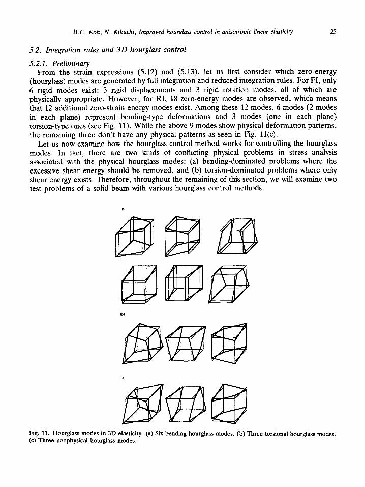
6 rigid modes exist: 3 rigid displacements and 3 rigid rotation modes, all of which are physically appropriate. However, for RI, 18 zero-energy modes are observed, which means that 12 additional zero-strain energy modes exist. Among these 12 modes, 6 modes (2 modes in each plane) represent bending-tie deformations and 3 modes (one in each plane) torsion-type ones (see Fig. 11). While the above 9 modes show physical deformation patterns, the remaining three don’t have any physical patterns as seen in Fig. 11(c).
Let us now examine how the hourglass control method works for controlling the hourglass modes. In fact, there are two kinds of conflicting physical problems in stress analysis associated with the physical hourglass modes: (a) bending-dominated problems where the excessive shear energy should be removed, and (b) torsion-dominated problems where only shear energy exists. Therefore, throughout the remaining of this section, we will examine two test problems of a solid beam with various hourglass control methods.
Fig. 11. Hourglass modes in 3D elasticity. (a) Six bending hourglass modes. (b) Three torsional hourglass modes. (c) Three nonphysi~ai hourglass modes.
26 B.C. Koh, N. Kikuchi. Improved hourglass control in anisotropic linear elasticity
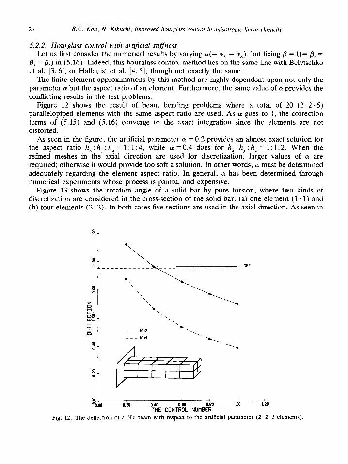
5.2.2. Hourglass control with artificial stiffness Let us first consider the numerical results by varying a(= (TV = as), but fixing p = l(= p, =
p, = /3,) in (5.16). Indeed, this hourglass control method lies on the same line with Belytschko et al. [3,6], or Hallquist et al. [4,5], though not exactly the same.
The finite element approximations by this method are highly dependent upon not only the parameter (Y but the aspect ratio of an element. Furthermore, the same value of (Y provides the conflicting results in the test problems.
Figure 12 shows the result of beam bending problems where a total of 20 (2 * 2.5) parallelopiped elements with the same aspect ratio are used. As (Y goes to 1, the correction terms of (5.15) and (5.16) converge to the exact integration since the elements are not distorted.
As seen in the figure, the artificial parameter (Y = 0.2 provides an almost exact solution for the aspect ratio h, . -h,:h, =1:1:4, while (~=0.4 does for h,:h,:hZ=1:1:2. When the refined meshes in the axial direction are used for discretization, larger values of (Y are required; otherwise it would provide too soft a solution. In other words, (Y must be determined adequately regarding the element aspect ratio. In general, (Y has been determined through numerical experiments whose process is painful and expensive.
Figure 13 shows the rotation angle of a solid bar by pure torsion, where two kinds of discretization are considered in the cross-section of the solid bar: (a) one element (1.1) and (b) four elements (2 - 2). In both cases five sections are used in the axial direction. As seen in
\ \ \ \ ‘\
‘x - 1:1:2 --_
4
I 0.20 0.40
THE CONT:fL N”“&i i.m 1.20
Fig. 12. The deflection of a 3D beam with respect to the artificial parameter (2.2.5 elements).

B.C. Koh, N. Kikuchi, Improved hourglass control in anisotropic linear elasticity 27
8_ i
8.. m’
\ _ 1~5 ELEHENTS
2~2~5 ELENENTS
Fig. 13. The normalized rotation angle of a solid beam with respect to the control parameters.
the figure, refined meshes in the cross-section of a bar are required to obtain converged results in torsional deformation. When cy = 0.4, which is considered rather stiff in bending (in Fig. 11)) the discretization of the case (b) gives 15% error, but the first case gives an unreasonable solution. And the small range of Q! (e.g. 0.1-0.2) which may be good for bending cases suffers too much ‘softening’ in torsion.
Indeed, it can be stated from these examples that even if a certain parameter is successfully chosen for a certain problem with a specific discretization, the method with cy cannot guarantee the same quality of approximation for other cases.
5.2.3. Hourglass control with SRI The hourglass control method following SRI segregates the volumetric and the shear strain
as in (3.27), and evaluates them only at the centroid in order to avoid ‘locking’ phenomena. Volumetric locking for incompressible material can be alleviated by underevaluating
volumetric strain as discussed before. Here the investigation on incompressibility won’t be elaborated any more since SRI on volumetric strain evaluates shear strain exactly and doesn’t carry any hourglass behavior.
Shear locking for bending cases can be solved by applying SRI on shear strain. However, as discussed for 2D, this approach fails to remove shear locking when an element is rotated. This difficulty can be overcome by executing SRI on shear strain with respect to the local (rotated) coordinate system rather than the global system, although the execution may endanger the advantage of hourglass control by increasing the number of computing operations drastically. Indeed, Example 6.3 of an arc ring subject to bending clearly demonstrates the effects of rotation on SRI.
Torsional hourglassing is another difficulty of hourglass control by SRI. Figure 13 also shows the torsional behavior by hourglass control on SRI with varying (Ye. Notice that (Ye of SRI provides the same results as (Y of artificial stiffness does; that is, a small value of (us gives too soft a result in pure torsion cases and if as = 0 (i.e., the strict SRI is applied), SRI can cause torsional hourglassing. Let us discuss more details on this situation, because torsional
28 B.C. Kc& N. Kikuchi, Improved hourglass control in anisotropic linear elasticity
hourglassing never happens in 2D and is the major difference between 2D and 3D. The strain vector can be decomposed with SRI as:
e = e,, + eN + cqS . (5.17)
where e, is the constant vector and eN and es are nonconstant strain vectors representing normal and shear strains, respectively. Indeed,
ek = {N,, E,,, ~z,O.O,O), e; = {O, O,O, ?fyzr N,,, N,,.} . where
(5.18)
(5.19)
and so on. Note that if cys = 0, (5.17) represent the strain by SRI; if cy = 1, (5.17) does by FI. From the orthogonality condition (5.11), it is easily shown that when cys = 0,
B l (C,h,, Czh2, C,h,) = 0, (5.21)
for a parallelpiped element. Note that (5.22) represents shear strains in torsional hourglass patterns in Fig. 11(b). In other words, torsional hourglassing can be activated in shear- dominated cases such as torsion. For bending-dominated cases this torsional hourglassing can be avoided without deteriorating the approximations, by putting a small number of (us such as 0.01. However, since bending and torsional deformations are extremely opposite regarding shear but can occur simultaneously in a structure, the underevaluation of shear strain must be taken carefully to avoid shear ‘-locking’ and ‘-softening’.
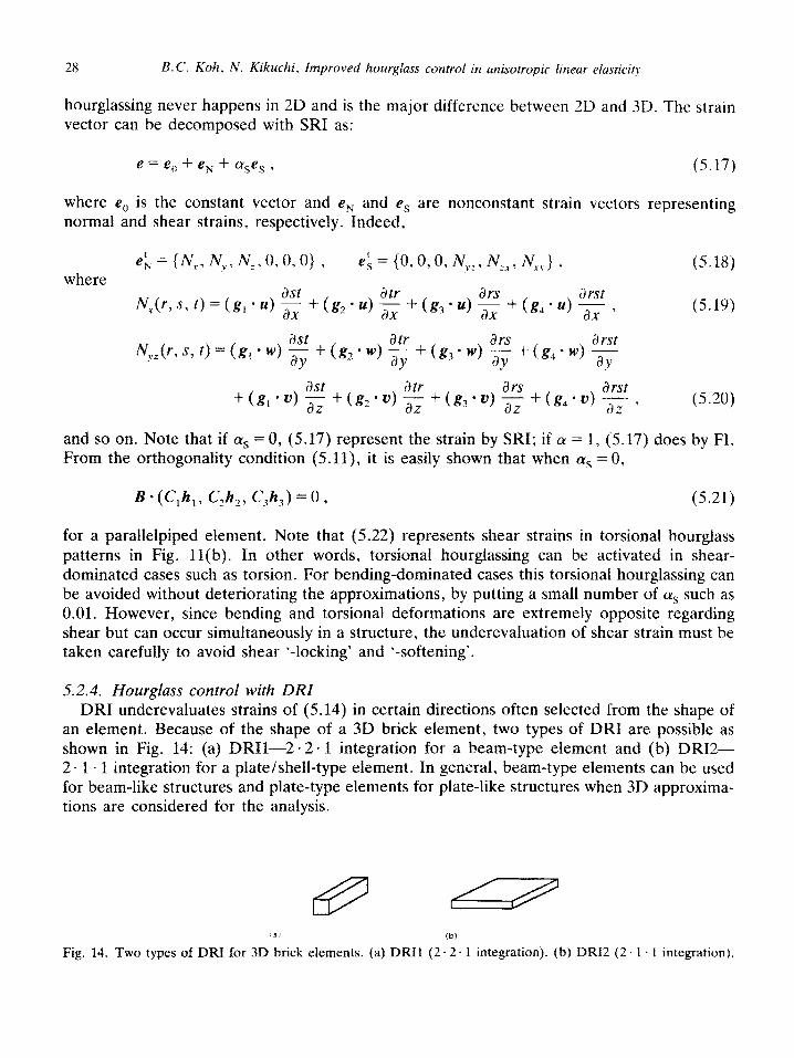
5.2.4. Hourglass control with DRI DRI underevaluates strains of (5.14) in certain directions often selected from the shape of
an element. Because of the shape of a 3D brick element, two types of DRI are possible as shown in Fig. 14: (a) DRIl-2 - 2 - 1 integration for a beam-type element and (b) DRI2- 2.1-l integration for a plate/shell-type element. In general, beam-type elements can be used for beam-like structures and plate-type elements for plate-like structures when 3D approxima- tions are considered for the analysis.
(3, (b) Fig. 14. Two types of DRI for 3D brick elements. {a) DRIl (2-2-l integration). (b) DR12 (2.1.1 integration).
B.C. Koh, N. Kikuchi, Improved hourglass control in anisotropic linear elasticity 29
Similarly to 2D, both DRIs solve effectively ‘shear locking’ in bending-dominated cases even for rotated elements. Example 6.3 of an arc ring clearly shows that DRIl provides good approximations in bending even with coarse meshes. Examples 6.4 of a plate and 6.6 of a deep shell demonstrate that DRI2 works well in both cases. Details of these will be given in Section 6.
Before discussing the results by DRI in torsional problems, let us consider how DRI evaluates strains in (5.14).
Suppose that a side, say in the r-direction, of a regular brick element is much longer than others as in Fig. 14(a). Then the strain in the r-direction is to be underintegrated by setting p, = 0 in (5.14) according to DRIl. That is,
e = e, + s e, + 4 e, + st e,, . Jcl Jcl Jcl
(5.22)
From the orthogonality of (5.11), it is not difficult to show that any hourglass vectors hi are not orthogonal to e of (5.23). Indeed, this fact means that any hourglassing never occurs with DRIl. In other words, since it evaluates in-plane shear nearly exactly (s-t plane in Fig. 14(a)), DRIl can avoid ‘shear softening’ of torsion in such a plane.
Now suppose that a side, say in the t-direction, of a plate/shell-type element is comparably smaller than others as in Fig. 14(b). (In a plate/shell element this side can be in the thickness direction.) Then, by setting /3, = /3, = 0, with DR12, (5.14) becomes
e = e, + 4 e, . Jo
(5.23)
That is, DR12 evaluates all in-plane shears only at the centroid in the plane (in this case, the T-S plane), and avoids shear locking in the plane. However, from (5.11) and (5.24))
B - (C,h, + C,h,, C,h, + C,h,, C,h, + C,h,) = 0. (5.24)
In other words, 6 hourglass modes can be activated by DR12 in certain cases, which is a drawback of DR12. Although, as in SRI, small numbers of p, and /I, can remove this hourglassing, the introduction of any artijicial number is not our intention of this study. Indeed, combining DRIl and DR12, we could overcome this difficulty without any artificial number so that numerical instability does not occur. Details on this technique will be discussed with
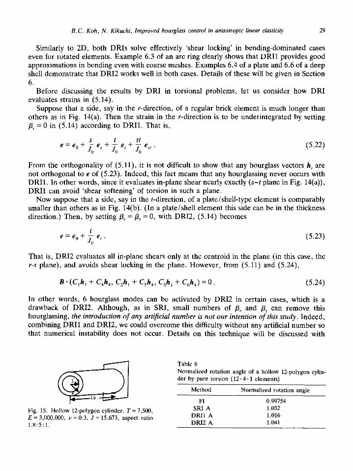
Fig. 15. Hollow 1Zpolygon cylinder. T = 7,500, E = 3,000,000, v = 0.3, J = 15.673, aspect ratio 1.8:5: 1.
Table 6 Normalized rotation angle of a hollow 1Zpolygon cylin- der by pure torsion (12.4.1 elements)
Method
FI SRI A
DRIl A DR12 A
Normalized rotation angle
0.99754 1.032 1.016 1.041
30 B.C. Koh, N. Kikuchi, Improved hourgiass control in anisotropic linear elasticity
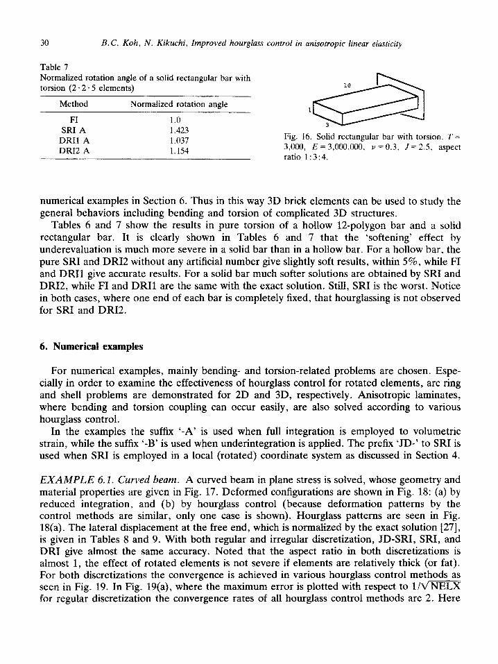
Table 7 Normalized rotation angle of a solid rectangular bar with torsion (2 * 2.5 elements)
Method
FI SRI A
DRIl A DR12 A
Normalized rotation angle
1.0 1.423 1.037 1.154
Fig. 16. Solid rectangular bar with torsion. T = 3,000, E=3,OOil,OOO, v =0.3, J=2.5. aspect ratio 1:3:4.
numerical examples in Section 6. Thus in this way 3D brick elements can be used to study the general behaviors including bending and torsion of complicated 3D structures.
Tables 6 and 7 show the results in pure torsion of a hollow 1Zpolygon bar and a solid rectangular bar. It is clearly shown in Tables 6 and 7 that the ‘softening’ effect by underevaluation is much more severe in a solid bar than in a hollow bar. For a hollow bar, the pure SRI and DR12 without any artificial number give slightly soft results, within 5%, while FI and DRIl give accurate results. For a solid bar much softer solutions are obtained by SRI and DR12, while FI and DRIl are the same with the exact solution. Still, SRI is the worst. Notice in both cases, where one end of each bar is completely fixed, that hourglassing is not observed for SRI and DR12.
6. Nurn~~~l examples
For numerical examples, mainly bending- and torsion-related problems are chosen. Espe- cially in order to examine the effectiveness of hourglass control for rotated elements, arc ring and shell problems are demonstrated for 2D and 3D, respectively. Anisotropic laminates, where bending and torsion coupling can occur easily, are also solved according to various hourglass control.
In the examples the suffix ‘-A’ is used when full integration is employed to volumetric strain, while the suffix “-B’ is used when underintegration is applied. The prefix ‘JD-’ to SRI is used when SRI is employed in a local (rotated) coordinate system as discussed in Section 4.
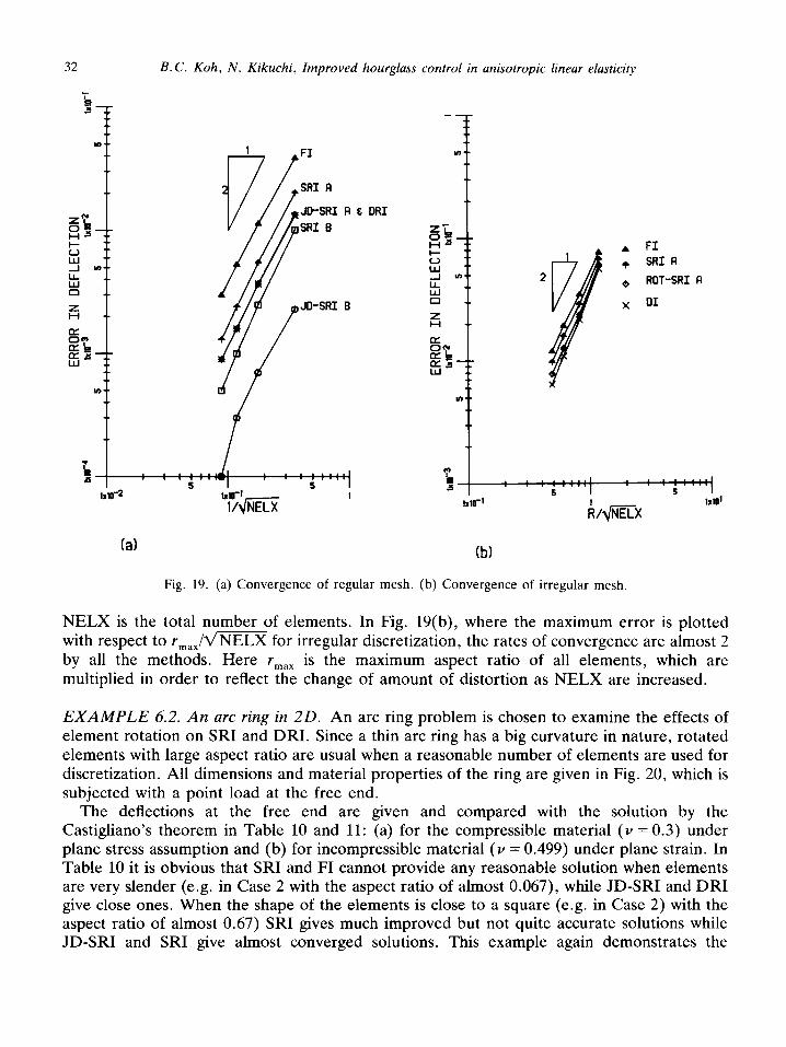
~XA~P~~ 6.1. Curved beam. A curved beam in plane stress is solved, whose geometry and material properties are given in Fig. 17. Deformed configurations are shown in Fig. 18: (a) by reduced integration, and (b) by hourglass control (because deformation patterns by the control methods are similar, only one case is shown). Hourglass patterns are seen in Fig. 18(a). The lateral displacement at the free end, which is normalized by the exact solution [27], is given in Tables 8 and 9. With both regular and irregular discretization, JD-SRI, SRI, and DRI give almost the same accuracy. Noted that the aspect ratio in both discretizations is almost 1, the effect of rotated elements is not severe if elements are relatively thick (or fat). For both discretizations the convergence is achieved in various hourglass control methods as seen in Fig. 19. In Fig. 19(a), where the maximum error is plotted with respect to l/m for regular discretization the convergence rates of all hourglass control methods are 2. Here
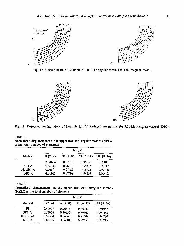
B.C. Koh, N. Kikuchi, Improved hourglass control in anisotropic linear elasticity 31
*P-40.000
(a)
Fig. 17. Curved beam of Example 6.1 (a) The regular mesh. (b) The irregular mesh.
Fig. 18. Deformed configurations of Example 6.1. (a) Reduced integration. (9 RI with hourglass control (DRI).
Table 8 Normalized displacements at the upper free end, regular meshes (NELX is the total number of elements)
NELX
Method 8 (2.4) 32 (4 + 8) 72 (6.12) 128 (8.16)
FI 0.74624 0.92317 0.96606 0.98011 SRI-A 0.86344 0.96319 0.98378 0.99112
JD-SRI-A 0.9080 0.97489 0.98905 0.99406 DRI-A 0.91061 0.97498 0.98899 0.99402
Table 9 Normalized displacements at the upper free end, irregular meshes (NELX is the total number of elements)
NELX
Method 8 (2.4) 32 (4.8) 72 (6.12) 128 (8.16)
FI 0.40907 0.76313 0.86942 0.91947 SRI-A 0.55004 0.80630 0.89362 0.93463
JD-SRI-A 0.59384 0.84060 0.91509 0.94780 DRI-A 0.62365 0.84984 0.92650 0.95715
B.C. Koh, N. Kikuchi, Improved hourglass control in anisotropic linear elasticity
I FI
SRI R
JD-SRI SRI B
JO-SRI
A E DRI
B
(a)
FI SRI
ROT-
01
R
-SRI A
(b)
Fig. 19. (a) Convergence of regular mesh. (b) Convergence of irregular mesh
NELX is the total number of elements. In Fig. 19(b), where the maximum error is plotted with respect to rmax /m for irregular discretization, the rates of convergence are almost 2 by all the methods. Here rmax is the maximum aspect ratio of all elements, which are multiplied in order to reflect the change of amount of distortion as NELX are increased.
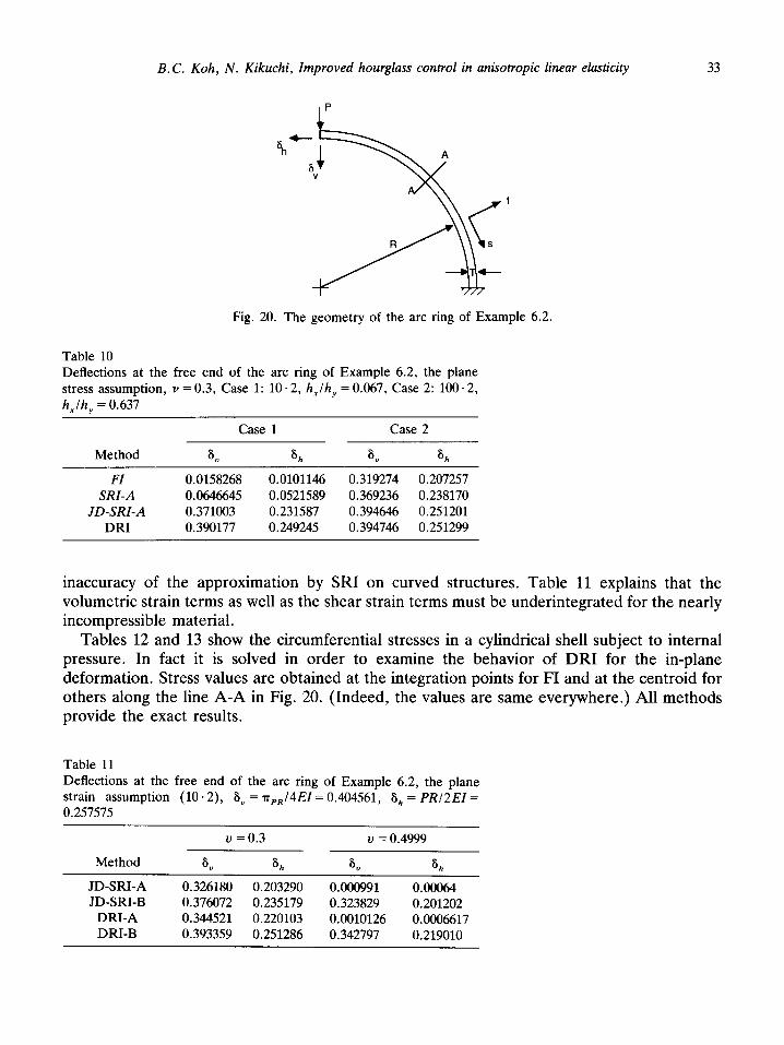
EXAMPLE 6.2. An arc ring in 20. An arc ring problem is chosen to examine the effects of element rotation on SRI and DRI. Since a thin arc ring has a big curvature in nature, rotated elements with large aspect ratio are usual when a reasonable number of elements are used for discretization. All dimensions and material properties of the ring are given in Fig. 20, which is subjected with a point load at the free end.
The deflections at the free end are given and compared with the solution by the Castigliano’s theorem in Table 10 and 11: (a) for the compressible material (V = 0.3) under plane stress assumption and (b) for incompressible material (V = 0.499) under plane strain. In Table 10 it is obvious that SRI and FI cannot provide any reasonable solution when elements are very slender (e.g. in Case 2 with the aspect ratio of almost 0.067), while JD-SRI and DRI give close ones. When the shape of the elements is close to a square (e.g. in Case 2) with the aspect ratio of almost 0.67) SRI gives much improved but not quite accurate solutions while JD-SRI and SRI give almost converged solutions. This example again demonstrates the
B.C. Koh, N. Kikuchi, Improved hourglass control in anisotropic linear elasticity 33
Fig. 20. The geometry of the arc ring of Example 6.2.
Table 10 Deflections at the free end of the arc ring of Example 6.2, the plane stress assumption, Y = 0.3, Case 1: 10.2, h,lh, = 0.067, Case 2: 100 *2, h,lh, = 0.637
Method
Case 1 Case 2
6” 6, 6” %
FI 0.0158268 0.0101146 0.319274 0.207257 SRI-A 0.0646645 0.0521589 0.369236 0.238170
JD-SRI-A 0.371003 0.231587 0.394646 0.251201 DRI 0.390177 0.249245 0.394746 0.251299
inaccuracy of the approximation by SRI on curved structures. Table 11 explains that the volumetric strain terms as well as the shear strain terms must be underintegrated for the nearly incompressible material.
pressure. In fact it is solved in order to examine the deformation. Stress values are obtained at the integration others along the line A-A in Fig. 20. (Indeed, the values provide the exact results.
Tables 12 and 13 show the circumferential stresses in a cylindrical shell subject to internal behavior of DRI for the in-plane points for FI and at the centroid for are same everywhere.) All methods
Table 11 Deflections at the free end of the arc ring of Example 6.2, the plane strain assumption (10 * 2), 6, = n,,/4EI = 0.404561, 6, = PRI2EI = 0.257575
u = 0.3 u = 0.4999
Method 6” 6, 8” 6,
JD-SRI-A 0.326180 0.203290 0.000991 0.00064 JD-SRI-B 0.376072 0.235179 0.323829 0.201202
DRI-A 0.344521 0.220103 0.0010126 0.0006617 DRI-B 0.393359 0.251286 0.342797 0.219010

34 B.C. Koh, N. Kikuchi, Improved hourglass control in anisotropic linear elasticity
Table 12 Hoop stresses along A-A in the arc ring with internal pressure q = 100 (the elementary solution pee = %OO), 100.2 elements
Method Stress Remarks
FI
SRI JD-SRI
DRI
1 5050.41 Stresses are evaluated at the 2 4999.15 integration points along the 3 4999.74 thickness direction. The first 4 4950.13 one is at the most inside point
1 5024.76 At the centroid
2 4974.91
Table 13 Hoop stresses along A-A in the arc ring with internal pressure q = 100 (the elementary solution a,, = SOOO), 10 * 2 elements
Method Stress Remarks
DRI 1 5024.76 At the centroid 2 4974.91
(a)
(b)
Fig. 21. Arc ring with 3D model of Example 6.3. (a) Model. (b) Deformed shape by DRII.

B.C. Koh, N. Kikuchi, Improved hourglass control in anisotropic linear elasticity 35
Fig. 22. One quarter of the plate of Example 6.4. a = 10, t = 0.2, E = 30,000,000, case), q = -100 (simply-supported case).
(4
l SRIR 0
t
v = 0.3, P = -10,ooO (clamped
Fig. 23. The results of a clamped plate with a point load, P = 40,000. (a) Convergence, (b) deflection at the center.

36 B.C. Koh. N. Kikuchi, Improved hourglass control in anisotropic linear elasticity
Table 14 Deflections at the free end of the arc ring by using 3D brick elements (2.2. 10 elements)
SRI-A JD-SRI-A DRIl-A Exact
61, 0.049287 0.226016 0.24577 0.257575
6. 0.061606 0.364541 0.38480 0.404561
Fig. 24. The deflection along the centerline of a simply-supported plate with uniform pressure (q = 100).
EXAMPLE 6.3. An arc ring in 30. The same arc ring problem is repeated by using 3D elements. The cross-section of the ring is an unit square, and discretized into 4 sections as seen Fig. 21(a). Deformed shapes are shown in Fig. 21(b) and deflections at the free end are given in Table 14, where DRI gives clearly the best solution.
EXAMPLE 6.4. Plate bending problem. The plate bending problem is the first natural choice of the study of hourglass control for 3D problems. Both the clamped and the simply-supported cases are solved. The dimensions and material properties of the plate as well as its discretization are given in Fig. 22. Only one quarter of the plate is solved because of its symmetry. A point load is applied at the center for the clamped case and a uniform load for simply-supported case. Since each discretized element is the plate type, DR12 is used for the DRI method.
Table 1.5 Deflections at the center of a simply-supported square plate, exact solution w = 8.4448 by [27], Case 1: thin ‘layers’ are added along the center lines as in Fig. 25. Case 2: thin ‘layers’ are added along the boundary
NELX Case 1
5.5.1 6.90045
5.5.2 8.11866 5.5.4 8.4937
Case 2
_
8.2356 8.5033
B.C. Koh, N. Kikuchi, Improved hourglass control in anisotropic linear elasticity 31
b)
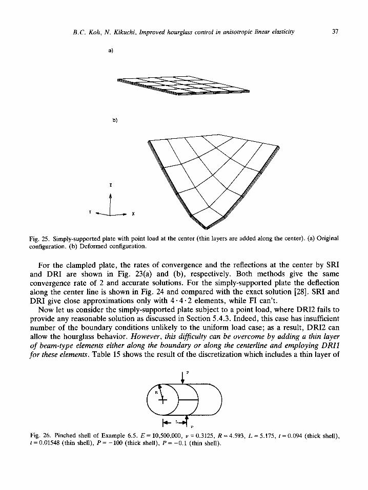
Fig. 25. Simply-supported plate with point load at the center (thin layers are added along the center). (a) Original configuration. (b) Deformed configuration.
For the clampled plate, the rates of convergence and the reflections at the center by SRI and DRI are shown in Fig. 23(a) and (b), respectively. Both methods give the same convergence rate of 2 and accurate solutions. For the simply-supported plate the deflection along the center line is shown in Fig. 24 and compared with the exact solution [28]. SRI and DRI give close approximations only with 4 - 4 - 2 elements, while FI can’t.
Now let us consider the simply-supported plate subject to a point load, where DR12 fails to provide any reasonable solution as discussed in Section 5.4.3. Indeed, this case has insufficient number of the boundary conditions unlikely to the uniform load case; as a result, DR12 can allow the hourglass behavior. However, this dijj’kulty can be overcome by adding a thin layer of beam-type elements either along the boundary or along the centerline and employing DRIl for these elements. Table 15 shows the result of the discretization which includes a thin layer of
P
R @P k-L P
Fig. 26. Pinched shell of Example 6.5. E = 10,500,000, Y = 0.3125, R = 4.593, L = 5.175, t = 0.094 (thick shell), t = 0.01548 (thin shell), P = -100 (thick shell), P = -0.1 (thin shell).

38 B.C. Koh, N. Kikuchi, Improved hourglass control in anisotropic linear elasticity
a)
a)
Fig. 27. Configuration of the thin shell of Example 6.5. (a) Original configuration. (b) Deformed configuration (50 times multiplied).
elements. Note that in this case all kinds of integration rules - FI, DRIl, and DRI2 - are used together, and determined by the ratio of the sides of each element: for example, if an element is almost a cube, then FI is employed, and if an element is like a beam, then DRIl is used. Despite the use of FI and DRIl on the thin layer, those tiny elements appear not to disturb the main physical phenomenon -bending deformation. It should be noted that better solutions are obtained when the thin layer is added along the boundary rather than the center line. Figure 25 shows the original and deformed configurations of this case.
EXAMPLE 6.5. Shell with a pinched load. Two cases of a cylindrical shell subject to a pinched load are solved: (a) for a thick shell, where t/R = &, and (b) for a thin shell, where t/R = &. Detailed dimensions and material properties are given in Fig. 26. Because of the symmetry, one eighth of the geometry is discretized into is shown in Fig. 27.
Fig. 28. Anti-symmetric laminate of Example 6.6. E, = 21 x lo”, E, = 2.1 X 10⁶, G,, = G,, = G,, = 0.85 X 10⁶,
%z = %3 = v3, = 0.21, resultant extensional force N, = 25,000, thickness of each lamina t = 0.1.
B.C. Koh, N. Kikuchi, Improved hourglass control in anisotropic linear elasticity 39
Table 16 Deflections of thick shell with a pinched load (10 * 10.2 brick elements are used; for DRI, layer elements are added), load P = -100
JD-SRI-A JD-SRI-B DRI-A DRI-B Remarks
0.10553 0.12190 0.10554 0.12161 0.1137” 0.09500 0.10943 0.09504 0.10962 -
a By Ashwell and Sabir [25].
Table 17 Deflections of thin shell with a pinched load (10 * 10 * 2 brick elements are used; for DRI, larger elements are added), load P = -0.1
JD-SRI-A JD-SRI-B DRI-A DRI-B Remarks
6” 0.01396 0.01805 0.02269 0.02606 0.02432” 6, 0.01344 0.01724 0.02077 0.02393 0.02236”
a By the inextensible theory [27].
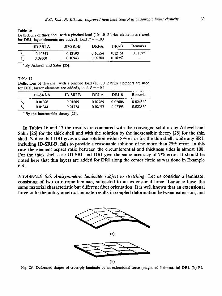
In Tables 16 and 17 the results are compared with the converged solution by Ashwell and Sabir [26] for the thick shell and with the solution by the inextensible theory [285 for the thin shell. Notice that DRI gives a close solution within 8% error for the thin shell, while any SRI, including JD-SRI-B, fails to provide a reasonable solution of no more than 25% error. In this case the element aspect ratio between the circumferential and thickness sides is almost 100. For the thick shell case JD-SRI and DRI give the same accuracy of 7% error. It should be noted here that thin layers are added for DRI along the center circle as was done in Example 6.4.
EXAMPLE 6.6. Antisymmetric laminates subject to stretching. Let us consider a laminate, consisting of two ortotropic laminae, subjected to an extensional force. Laminae have the same material characteristic but different fiber orientation. It is well known that an extensional force onto the antisymmetric laminate results in coupled deformation between extension, and
(4
(b) Fig. 29. Deformed shapes of cross-ply laminate by an extensional force (magnified 5 times). (a) DRI. (b) FI.

40 B.C. Koh, N. Kikuchi, Improved hourglass control in anisotropic linear elasticity
(4
Fig. 30. Deformed shapes of 30” angle-ply laminate by an extensional force (magnified 5 times). (a) DRI. (b) Fl.
(a) O’* 1
s ‘;;
3 0.1
zi
I
- wby DRI
+ wbyFI
+ u by DRI
-X- ubyFI
0.0 ,~
0 1 2 3 4 5
X
lb)
0.3
0.2
0.1
s
3 0.0
2 -0.1
-0.2
1
-0.3 I
0 1 2 3 4 5
Fig. 31. Deflections along the end of the middle plane ‘of the laminate of Example 6.6. u and w denote the extension and deflection, respectively. (a) Cross-ply laminate, (b) 30” angle-ply laminate.
B.C. Koh, N. Kikuchi, Improved hourglass control in anisotropic linear elasticity 41
twisting or bending 1301. In this example, antisymmetric cross-ply and 30” angle-ply are solved. The geometry and material properties are given in Fig. 28. While the cross-ply laminate force has a coupled deformation between extension and bending, the angle-ply has a coupled deformation between extension and twisting.
The deformed configurations by FI and DRI are shown in Figs. 29 and 30 for both cases and the amount of deflection and extension along the end of the middle plane in the extensional direction, see Fig. 31. While for the angle-ply laminate almost the same amounts of twisting are obtained by FI and DRI, the significant differences in deflections are observed for the cross-ply laminate. This can be quite expected because FI suffers shear locking in bending for the cross-ply. Note that in both cases the extensional deformations are not so significant as the bending or twisting deformations. Here ‘thin-layer’ elements are used along the boundary of the laminate.
7. Conclusions and discussions
In this paper hourglass control is developed as the correction of the reduced integration scheme which does not introduce any kind of artificial control parameters. To achieve this goal the algebraic relation between the physical element and the master element is used. In this way hourglass control (thus the resulting explicit algorithm) can be extended to evaluate any terms in the virtual displacement formulation employing bi- or trilinear isoparametric interpo- lation; the advantage of hourglass control can be exploited more.
The study is performed in consideration of not only the shape of the element such as aspect ratio, element rotation, and distortion but also of the physical point for linear elasticity. Especially, since the shear in the linear elasticity is found to play conflicting roles in bending and torsion, hourglass control must be performed based upon the physical consideration in 2D and 3D. The results are compared with ones by various existing hourglass control methods with artificial parameter or integration schemes such as selective reduced integration (SRI) and directional reduced integration (DRI).
Hourglass control with an artificial parameter is found to be so sensitive not only to the parameter but to the aspect ratio of an element that it must be taken depending on the discretization. Thus the judgement of the appropriate number for the parameter could be difficult and costly. It also fails to give the same quality of approximation between bending and torsion in 3D with the same value of the parameter.
Hourglass control with SRI on shear provides a good approximation on bending without introducing any artificial parameters. However, this performance is limited on the rather thick and less ‘rotated (skewed)’ elements. It was found that the error by the SRI method is the maximum when an element is rotated at 45” to the physical coordinate system, and it becomes much more severe when an element is long and thin. This is because SRI cannot reflect the real stress distribution for such cases. Another drawback of the method is ‘shear softening’ in torsion which results from underintegration to shear. Therefore, the underintegration on the material properties must be taken carefully.
Hourglass control with DRI resolves the difficulties by hourglass control with SRI success- fully without introducing any artificial number. In DRI the underevaluation to strains is determined by the geometry of element rather than by the physical component. Thus DRI is

42 B.C. Koh, N. Kikuchi. Improved hourglass control in anisotropic linear elasticit!
insensitive to the element rotation and solves shear-related difficulties. Using DRI even a thin and deeply curved structure (such as an arch) can be solved with the continuum approach as well as the plate/shell structures. It could be better to determine the direction to the underevaluated a posteriori rather than a priori as currently used by the element geometry, because even the slender bending-type element may not be under bending or even a square element may be under bending. The gradient of stresses could be a possible a posteriori criterion. This attempt is currently tried successfully when an element is relatively regular. We believe that this study must follow the thorough physical understanding of the ‘locking’ phenomenon.
While hourglass control with DRI has been found to perform well for controlling shear locking, hourglass control with DRI must be implemented with the underevaluation on volumetric strain for controlling volumetric locking which comes from the incompressibility of the material because it is performed based on only the information of the element geometry. The mathematical proof of DRI is not carried out in this paper: however, the convergence of DRI is achieved in the numerical examples with both regular and irregular meshes.
As a byproduct of this study, a distortion indicator on element is defined by decomposing the Jacobian matrix into rotation and distortion matrices, and the effect of element distortion on hourglass control is examined. Through numerical experiments, a reasonable approxima- tion may be assured by limiting the distortion indicator to less than 0.2. This information can be used for discretization to enhance the numerical approximation.
Appendix A. A gradient matrix B for a plane strain case
For a Q4 element a gradient matrix B can be decomposed into constant and linear parts,
B = B, + Blin , (A-1)
where B, and Blzn represent constant and linear gradient matrices, respectively. Indeed, B, is the same gradient matrix obtained by RI and Btin is an additional matrix by hourglass control. Blin can also be decomposed into (1) deviatoric-normal, shear, and volumetric parts by following SRI, or (2) s- and t-directional parts by following DRI. That is,
(A.2)
where all the subscripts are defined as in Section 3. cys and /3s are the control parameters which are assigned 0 where the undeintegration is needed or 1 where the full integration is needed. The values of the parameters are determined by he corresponding hourglass control method.
For the plane strain case, all Bs in (A.2) are expressed explicitly as following:
(A.31
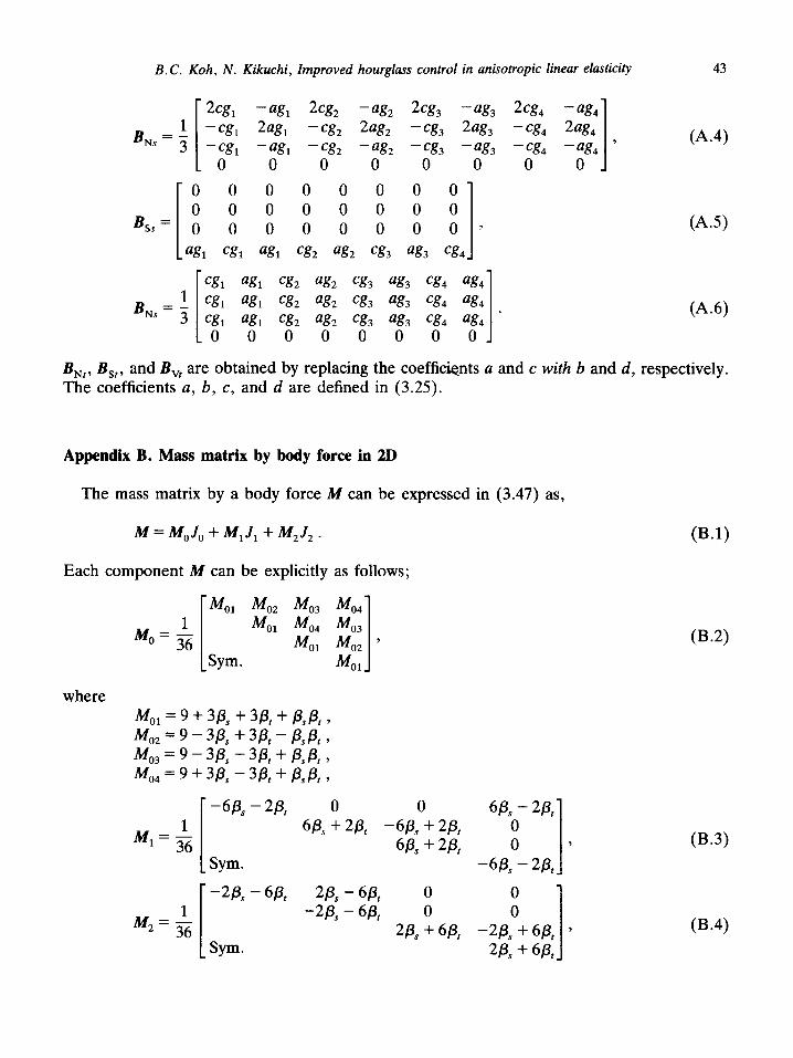
B.C. Koh, N. Kikuchi, Improved hourglass control in anisotropic linear elasticity 43
2% - ag, kg, -ag, 2cg3 -ag3 2Cg4 --a&
1
44s = j -cg, 2ag, - cg, Zag, - q3 zag, -cg4 zag4 -cg1 -a&J, - C82 - at?2 - cg3 - ag, - %I -al?, ’ 64)
0 0 0 0 0 0 0 0 1
i
0 0 0 0 0 0 0 0 0 0 0 0 0 0 0 0
Bss= 0 0 0 0 0 0 0 0
ag1 cg, ag, cg2 ag2 cg3 ag3 cg4 I ’ (A3
ag1 cg, ag2 cg3 ag3 cg4 ag4
ag, cg, ag, cg3 ag3 Cg4 ag4
agl cg, ag2 cg3 ag3 cg4 ag4 * 64.6)
0 0 0 0 0 0 0 0 I
BN,, Bst , and B, are obtained by replacing the coefficients a and c with b and d, respectively. The coefficients a, b, c, and d are defined in (3.25).
Appendix B. Mass matrix by body force in 2D
The mass matrix by a body force M can be expressed in (3.47) as,
M = MoJ,, + M, J1 + M2J2 .
Each component M can be explicitly as follows;
where M,, = 9 + 3p, + 3P, + PA 9
MO2 = 9 - 3& + 3& - && 9 MO3 = 9 -3p, - 3P, + P,P, 3 MO4 = 9 + 3p, - 3P, + PA 3
MI = I
-6P, - 2P, 0 0 W, - 28 1
W,
+
26
-
W,
+
2P,
0 36
Sym. -W, - 28 I
W,+2P, o ’
-2P, - W 2P, - W, 0 0 1 M2=36 -2P, -W, 0 0
33, + wt -W,+W, ’
Sym. 2& + W, I
(B-1)
(B-2)
P-3)
(B.4)
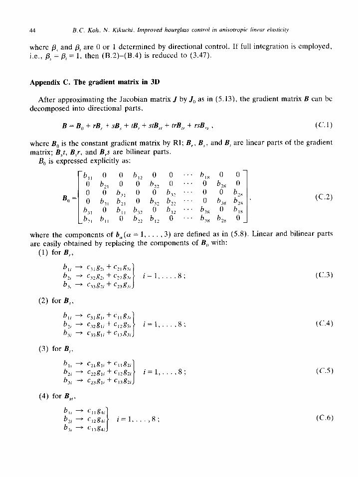
44 B.C. Koh, N. Kikuchi. Improved hourglass control in anisotropic linear elasticity
where p,, and p, are 0 or 1 determined by directional control. If full integration is employed, i.e., p, = p, = 1, then (B.2)-(B.4) is reduced to (3.47).
Appendix C. The gradient matrix in 3D
After approximating the Jacobian matrix J by Jo as in (5.13), the gradient matrix B can be decomposed into directional parts,
B = B, + T-B, + SB, + tB, + stB,, + trB,, + rsB,, 9 (C.1)
where B, is the constant gradient matrix by RI; B,, B,y, and B, are linear parts of the gradient matrix; B,t, Btr, and B,s are bilinear parts.
B,, is expressed explicitly as:
B, =
_b,, 0 0 b,, 0 0 * ** b,, 0 0 b,, 0 0 b23 0 . . . 0 bZ8 0 0 0 b,, 0 0 b,, ** * 0 0 0 b,, b2, 0 b,, b,, * * * 0 b,,
b .+. 31 0 b,, b32 0 b,2 b,, 0
b _ ?I b,, 0 b22 b,2 0 - -. b,, b,, 0
(C.2)
where the components of b, (a = 1, . . . , 3) are defined as in (5.8). Linear and bilinear parts are easily obtained by replacing the components of B,, with:
(I) for B,,
b,; + c31g3r + c21g3,
b 1, -+ ~32&+~22g.i, i=l,..., 8; (C.3)
b,, + ‘33g?i + ‘23g3i
(2) for B,,
bli + C31glr + Cllg3r bzi + C32gli + C12g3i i= 1,. . . ,8; (C.4)
b3i + c33gri + ci3g3i
(3) for B,,
4, + c21gli + cllgZi
b2i + C22gli + Cl2g2i
I
i=l,. . . ,8; b,i * c23gli + c13g2i
(4) for B,,,
b,i + Cllg4i b2i + ‘12g4i
I
i=l,. . . ,8;
b,i + C13g4i
(C.5)
(C.6)
B.C. Koh, N. Kikuchi, improved hourglass control in anisotropic linear elasticity 45
(5) for BIT,
bli + ‘21g4i
b2i + ‘22g4i i=1,...,8; b3i + ‘23g4i
(C-7)
(6) for B,,,
bli * ‘3lg4i
b2i * ‘32g4i i=l,. . . ,8; (C.8) b3i + ‘33g4i
where the components of g, ((Y = 1, . . . ,4) are given in (5.9) and the coefficients cI1, . . . , c33
in (5.6)
References
[l] G. Maechnen and S. Sack, The tensor code, in: B. Alder et al., eds., Methods of Computational Physics (Academic Press, New York, 1964) 181-260.
[2] S.W. Key, HONDO-A finite element computer program for the large deformation dynamic response of axisymmetric solids, R.74-0039, Sandia National Laboratories, Albuquerque, NM, 1974.
[3] D.P. Flanagan and T. Belytschko, A uniform strain hexahedron and quadrilateral with orthogonal hourglass control, Internat. J. Numer. Meths. Engrg. 17 (1981) 696-706.
[4] G.L. Goudreau and J.O. Hallquist, Rec&t developments in large-scale finite element Lagrangian hydrocode technology, Comput. Meths. Appl. Mech. Engrg. 33 (1982) 725-757.
[S] J.O. Hallquist, Theoretical manual for DYNA3D, UCID-19401 Lawrence Livermore National Lab, Universi- ty of California (1983) 19-20.
[6] T. Belytschko, J.S. Ong, W.K. Liu and J.D. Kennedy, Hourglass control in linear and nonlinear problems, Comput. Meths. Appl. Mech. Engrg. 43 (1984) 251-276.
[7] O.P. Jacquotte and J.T. Oden, Analysis of hourglass instabilities and control in underintegrated finite element methods, Comput. Meths. Appl. Mech. Engrg. 44 (1984) 339-363.
[8] O.P. Jacquotte, Stability, accuracy, and efficiency of some underintegrated methods in finite element computations, Comput. Meths. Appl. Mech. Engrg. 50 (1985) 275-293.
[9] O.P. Jacquotte, J.T. Oden and E.B. Becker, Numerical control of the hourglass instability, Internat. J. Numer. Meths. Engrg. 22 (1986) 219-228.
[lo] J.C. Schulz, Finite element hourglassing control, Internat. J. Numer. Meths. Engrg. 21 (1985) 1039-1048. [ll] W.K. Liu, J.S. Ong and R.A. Uras, Finite element stabilization matrices - a unification approach, Comput.
Meths. Appl. Mech. Engrg. 53 (1985) 13-46. [12] T. Belytschko and W.E. Bachrach, Simple quadrilaterals with high coarse mesh accuracy, AMD-73, ASME,
New York (1985) 39-56. [13] W.E. Bachrach, W.K. Liu and R.A. Uras, Consolidation of various approaches in developing naturally based
quadrilateral, Comput. Meths. Appl. Mech. Engrg. 55 (1986) 43-62. [14] R.D. Cook and Z.H. Feng, Control of spurious mode in the nine node quadrilateral element, Internat. J.
Numer. Meths. Engrg. 18 (1982) 1576-1580. [15] N. Kikuchi, Finite Element Methods in Mechanics (Cambridge University Press, Cambridge, 1986). [16] D.M. Malkus and T.J.R. Hughes, Mixed finite element methods-reduced and selective integration tech-
niques: a unification concepts, Comput. Meths. Appl. Mech. Engrg. 15 (1978) 63-82. [17] T.J.R. Hughes, Equivalence of finite elements for nearly incompressible material, J. Appl. Mech. 44 (1977)
181-183.
46 B.C. Koh, N. Kikuchi, Improved hourglass control in anisotropic linear elasticity
[18] T.J.R. Hughes, Generalization of selective reduced integration procedures to anisotropic nonlinear media, Internat. J. Numer. Meths. Engrg. 15 (1980) 1413-1418.
[19] J.T. Oden and N. Kikuchi, Finite element methods for constrained problems in elasticity, Internat. J. Numer. Meths. Engrg. 18 (1982) 701-725.
[20] R.L. Taylor, P.J. Beresford and E.L. Wilson. A nonconforming element for stress analysis, Internat. J. Numer. Meths. Engrg. 18 (1976) 1211-1219.
[21] O.C. Zienkiewicz, R.L. Taylor and J.M. Too, Reduced integration technique in general analysis of plates and shells, Internat. J. Numer. Meths. Engrg. 18 (1971) 275-290.
[22] S.T. Pawsey and R.W. Clough, Improved numerical integration of thick shell finite elements, Internat. J. Numer. Meths. Engrg. 3 (1971) 56.5-586.
[23] H. Takemoto and R.D. Cook, Some modifications of an isoparametric element, Internat. J. Numer. Meths. Engrg. 3 (1973) 401-405.
[24] T.J.R. Hughes, R.L. Taylor and W. Kanoknukulchai, A simple and efficient finite element for plate bending, Internat. J. Numer. Meths. Engrg. 11 (1977) 1529-1543.
[25] W.K. Liu, T. Belytschko. J.S. Ong and S.E. Law, Use of stabilization matrices in non-linear analysis. Engrg. Comp. 2 (1985) 47-55.
[26] D.G. Ashwell and A.B. Sabir. A new cylindrical shell finite element based on simple independent strain functions, Internat. J. Mech. Sci. 44 (1972) 171-183.
[27] S.P. Timoshenko and J.N. Goodier, The Theory of Elasticity (Mcgraw-Hil, New York, 3rd ed., 1970). [28] S.P. Timoshenko and S. Woinowsky Krieger, Theory of Plates and Shells (Mcgraw-Hill, New York, 2nd ed..
1959). [29] O.C. Zienkiewicz, The Finite Element Method (Mcgraw-Hill, New York, 3rd. ed.. 1977). [30] R.M. Jones, Mechanics of Composite Materials (Mcgraw-Hill, New York, 1975).