Progress In Electromagnetics Research B, Vol. 71, 39–54, 2016

New Coupling Schemes for Distribution Broadbandover Power Lines (BPL) Networks

Athanasios G. Lazaropoulos*

Abstract—This paper considers the broadband performance of distribution broadband over power lines(BPL) networks when a new refined theoretical coupling scheme computation module (CS2 module)is applied. The broadband performance of distribution BPL networks is investigated in terms of theirchannel attenuation and capacity in the 3–88 MHz frequency range, which is the typical operatingfrequency band of BPL technology. The analysis and relevant numerical results outline the importantattenuation and capacity improvement of distribution BPL networks when CS2 module is applied.

1. INTRODUCTION

Similar to its original design, today’s power grid can become a suitable communications platform eitherfor providing broadband last mile access or for developing an advanced IP-based network with a myriadof smart grid applications when broadband over power lines (BPL) technology features are appliedacross it [1–9].

To examine the spectral behavior of distribution BPL networks — i.e., overhead and undergroundmedium-voltage (MV) and low-voltage (LV) BPL networks —, the hybrid model is also adopted inthis this paper. Extensively employed to examine the behavior of various multiconductor transmissionline (MTL) configurations in BPL networks [1–8, 10–16], the hybrid model is modular and consists of:(i) a bottom-up approach that is based on an appropriate combination of MTL theory and similaritytransformations; and (ii) a top-down approach that is based on the concatenation of multidimensionaltransmission matrices of the cascaded network BPL connections. During the top-down approach, acoupling scheme computation module defines the way that BPL signals are injected onto and extractedfrom the power lines of distribution BPL connections. Then, based on the hybrid model, several usefulbroadband performance metrics such as channel attenuation and capacity of the distribution BPLnetworks can be assessed when different coupling schemes are applied [2–7, 10, 17–19].

In this paper, a theoretical coupling scheme computation module (CS2 module) that defines a moregeneral and efficient version of the existing simple CS1 module is proposed. Actually, in comparison withCS1 module, CS2 module better exploits: (i) all the available conductors of the MTL configurationsso as to propose state-of-the-art coupling schemes with conductor participation percentage; and (ii)the injected and extracted power of signals at the transmitting and receiving ends of BPL connections.Therefore, CS2 module achieves better broadband performance metrics compared to the existing onessince it exceeds the today’s limitations of CS1 module through the use of the proposed BPL signalcoupling procedure of two interfaces.

The rest of this paper is organized as follows. In Section 2, the overhead and underground MV andLV MTL configurations as well as the respective indicative BPL topologies are demonstrated. On thebasis of the hybrid model, Section 3 synopsizes the basics of BPL signal propagation and transmission.Special attention is given to the role of coupling schemes and, especially, to CS2 module and its BPL

Received 15 August 2016, Accepted 18 October 2016, Scheduled 7 November 2016* Corresponding author: Athanasios G. Lazaropoulos (AGLazaropoulos@gmail.com).The author is with the School of Electrical and Computer Engineering, National Technical University of Athens, 9, Iroon PolytechneiouStreet, GR 15780, Zografou Campus, Athens, Greece.

40 Lazaropoulos

signal coupling procedure. Section 4 deals with electromagnetic interference (EMI) issues, noise andcapacity of distribution BPL networks. In Section 5, numerical results and discussion are provided,aiming at revealing the refreshing role of CS2 module; say, better channel attenuation and capacityperformance in comparison with the existing CS1 module. Section 6 concludes this paper.

2. DISTRIBUTION POWER GRIDS

2.1. Overhead MV and LV MTL Configuration

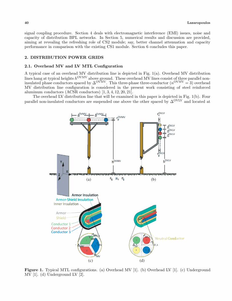
A typical case of an overhead MV distribution line is depicted in Fig. 1(a). Overhead MV distributionlines hang at typical heights hOVMV above ground. These overhead MV lines consist of three parallel non-insulated phase conductors spaced by ΔOVMV. This three-phase three-conductor (nOVMV = 3) overheadMV distribution line configuration is considered in the present work consisting of steel reinforcedaluminum conductors (ACSR conductors) [1, 3, 4, 12, 20, 21].

The overhead LV distribution line that will be examined in this paper is depicted in Fig. 1(b). Fourparallel non-insulated conductors are suspended one above the other spaced by ΔOVLV and located at

(a) (b)

(c) (d)

Figure 1. Typical MTL configurations. (a) Overhead MV [1]. (b) Overhead LV [1]. (c) UndergroundMV [1]. (d) Underground LV [2].

Progress In Electromagnetics Research B, Vol. 71, 2016 41

heights hOVLV above ground for the lowest conductor. The upper conductor is the neutral, while thelower three conductors are the three phases. This three-phase four-conductor (nOVLV = 4) overhead LVdistribution line configuration consists of ACSR conductors [1].

2.2. Underground MV and LV MTL Configuration

The UN MV distribution line that will be examined is the three-phase sector-type Paper Insulated LeadCovered (PILC) distribution-class cable depicted in Fig. 1(c). This cable arrangement consists of thethree-phase three-sector-type conductors (nUNMV = 3), one shield conductor and one armor conductorwhile the shield and the armor are grounded at both ends [1, 5, 22–24].

The UN LV distribution line that will be examined is the three-phase four-conductor (nUNLV = 4)core-type distribution cable depicted in Fig. 1(d). This cable arrangement consists of the three-phasethree-core-type conductors, one core-type neutral conductor and one shield conductor. Since there isno armor in this UN LV distribution line, only the shield is grounded at both ends [2, 13, 14, 21, 25, 26].

2.3. Ground and Reference Conductors

In all the cases examined, the conductivity of the ground is assumed σg = 5 mS/m and its relativepermittivity εrg = 13, which define a realistic scenario [1, 3, 4, 7, 10–12].

As it concerns the overhead distribution MTL configurations, the impact of imperfect ground onsignal propagation via overhead distribution power lines was analyzed in [2–7, 10–12, 20, 27–29]. Here,the ground is considered as the reference conductor.

As it concerns the underground distribution MTL configurations, the analytical formulation, whichis adopted in this paper, considers high frequency propagation in the general case of underground powerlines consisting of multiple conductors within common shield and analysed in [2, 5–7, 13, 14, 25, 30]. Here,the grounded shield is considered as the reference conductor.

2.4. Indicative Distribution BPL Topologies

To compensate the significant distance- and frequency-dependent attenuation of BPL signals, BPLnetworks are modified through the insertion of repeaters where a repeater is a device that boosts thedistance the BPL signal can propagate. Hence, BPL networks are divided into cascaded BPL connectionsthat are bounded by repeaters.

To apply the hybrid model, the simple BPL connection of Fig. 2(a) is considered. This simple BPLconnection is bounded by the transmitting end (repeater A) and receiving end (repeater B) while havingN branches. Since the number of branches differs depending on the examined connection, each BPLconnection is characterized by its BPL topology. To cope with different BPL topologies, the simple BPLconnection is assumed to be separated into segments (network modules) that comprise the successivebranches encountered — see Figs. 2(a) and 2(b) —. With reference to Fig. 2(c), the cascade of networkmodules corresponds to the topology of the BPL connection.

With reference to [1] and Fig. 2(a), average path lengths L = L1 + . . .+LN+1 of the order of 1000 mand 200 m are considered for overhead distribution — i.e., overhead MV and LV- and for undergrounddistribution — i.e., underground MV and LV-BPL connections, respectively.

As it concerns the overhead distribution BPL connections, five indicative overhead distributionBPL topologies of average path length, which are common for both overhead MV and overhead LVBPL connections, are examined. Their topological characteristics are detailed in Table 1. Similarlyto overhead distribution BPL connections, five indicative underground distribution BPL topologiesof average path length are examined in this paper. As in the overhead distribution BPL case, theunderground distribution BPL topologies are common for both underground MV and underground LVBPL connections and are detailed in Table 2.

The circuital parameters of the above indicative distribution BPL topologies are reported in [1–8, 10, 12, 14, 21, 22, 31–33]. Analytically, the cables of the branching lines are assumed identical to thedistribution ones while the interconnections between the distribution and branch lines are assumed tobe fully activated. The transmitting and the receiving ends are assumed matched to the characteristicimpedance of the distribution lines whereas the branch terminations are assumed open circuit.

42 Lazaropoulos

(a)

(b)

(c)

Figure 2. (a) End-to-end BPL connection with N branches. (b) Network module. (c) An indicativeBPL topology considered as a cascade of N + 1 modules corresponding to N branches [1].

Table 1. Overhead distribution BPL topologies.

Topology

Name

Topology

Description

Number

of

Branches

Length of

Distribution Lines

Length of

Branching Lines

Urban case ATypical overhead

urban topology3

L1 = 500 m, L2 = 200 m,

L3 = 100 m, L4 = 200 m

Lb1 = 8m,

Lb2 = 13m,

Lb3 = 10 m

Urban case B

Aggravated

overhead

urban topology

5

L1 = 200 m, L2 = 50 m,

L3 = 100 m, L4 = 200 m,

L5 = 300 m, L6 = 150 m

Lb1 = 12 m, Lb2 = 5 m,

Lb3 = 28 m, Lb4 = 41 m,

Lb5 = 17 m

Suburban caseOverhead suburban

topology2

L1 = 500 m, L2 = 400 m,

L3 = 100 mLb1 = 50m, Lb2 = 10 m

Rural caseOverhead rural

topology1 L1 = 600 m, L2 = 400 m Lb1 = 300 m

“LOS” case

Overhead

Line-of-Sight

transmission

0 L1 = 1000 m -

3. THE PRINCIPLES OF BPL SIGNAL PROPAGATION, TRANSMISSION ANDCOUPLING — THE HYBRID MODEL

3.1. Bottom-Up Approach

The first key element of the hybrid model is its bottom-up approach that deals with the signalpropagation across MTL configurations of distribution BPL networks. As it has already been

Progress In Electromagnetics Research B, Vol. 71, 2016 43

Table 2. Underground distribution BPL topologies.

Topology

Name

Topology

Description

Number

of

Branches

Length of

Distribution Lines

Length of

Branching Lines

Urban case ATypical underground

urban topology3

L1 = 70m, L2 = 55 m,

L3 = 45 m, L4 = 30 m

Lb1 = 12 m, Lb2 = 7m,

Lb3 = 21 m

Urban case B

Aggravated

underground

urban topology

5

L1 = 40m, L2 = 10 m,

L3 = 20m, L4 = 40 m,

L5 = 60 m, L6 = 30 m

Lb1 = 22 m, Lb2 = 12 m,

Lb3 = 8m, Lb4 = 2 m,

Lb5 = 17 m

Suburban caseUnderground

suburban topology2

L1 = 50 m, L2 = 100 m,

L3 = 50 mLb1 = 60 m, Lb2 = 30 m

Rural caseUnderground

rural topology1 L1 = 50 m, L2 = 150 m Lb1 = 100 m

“LOS” case

Underground

Line-of-Sight

transmission

0 L1 = 200 m -

mentioned in [1–7, 10, 11, 15], through a matrix approach, bottom-up approach can extend the standardtransmission line (TL) analysis to the MTL one, which involves more than two conductors. Similarlyto a two-conductor line where one forward- and one backward-traveling wave are supported, a MTLstructure with nG + 1 conductors may support nG pairs of forward- and backward-traveling waveswith corresponding propagation constants where [·]G denotes the examined power grid type — eitheroverhead MV or underground MV or overhead LV or underground LV — Each pair of forward- andbackward-traveling waves is referred to as a mode. Each of the nG modes propagates across BPLconnections while their spectral behavior has thoroughly investigated in [1–7, 10–15, 20, 21, 26–29].

3.2. Top-Down Approach

The second key element of the hybrid model is its top-down approach (i.e., TM2 method) that describesthe signal transmission across the BPL connections. TM2 method is based on the concatenationof multidimensional transmission matrices of the cascaded network BPL connections and presentedanalytically in [1]. In accordance with [1], the spectral behavior of the supported modes by each MTLconfiguration is described through the nG×nG eigenvalue decomposition (EVD) modal transfer functionmatrix Hm{·} whose elements Hm

i,j{·}, i, j = 1, . . . , nG are the EVD modal transfer functions where Hmi,j

denotes the element of the matrix Hm{·} in the row i of the column j.With reference to Figs. 3(a) and 3(b), the nG × nG channel transfer function matrix Hm{·} that

relates line voltages V(z) = [V1(z) · · · VnG(z)]T at the transmitting (z = 0) and the receiving (z = L)ends is determined from

H{·} = TV ·Hm{·} · T−1V (1)

where [·]T denotes the transpose of a matrix, and TV is a nG × nG matrix depending on the frequency,power grid type, physical properties of the cables and geometry of the MTL configuration.

3.3. CS2 Module, Its BPL Signal Coupling Procedure and Its Supported CouplingSchemes

According to how signals are injected onto and extracted from the lines of a MTL configuration, differentcoupling schemes may exist [1, 4, 7, 10–12]. With reference to Figs. 3(a) and 3(b), CS2 module describesthe BPL signal coupling procedure using two interfaces, namely:(1) BPL signal injection interface : It is located at the transmitting end — see Fig. 3(a) —.

Through the input coupling nG × 1 column vector Cin, this interface relates the line voltages

44 Lazaropoulos

(a) (b)

Figure 3. CS2 module. (a) BPL signal injection interface at the transmitting end. (b) BPL signalextraction interface at the receiving end.

V(0) = [V1(0) . . . VnG(0)]T with the input BPL signal V in+ through

V(0) = V in+ ·Cin (2)

The input BPL signal V in+ carries all the required information that needs to be transmittedthrough the BPL connection. The elements C in

i , i = 1, . . . , nG of the input coupling vector Cin

are the input coupling coefficients as well as the participation percentages of the conductors of theMTL configurations during the BPL signal injection; the sum of their absolute values is equal toone while their signs indicate the propagation direction of BPL signal.

(2) BPL signal extraction interface: It is located at the receiving end — see Fig. 3(b) — and, throughits output coupling 1 × nG line vector Cout = [Cout

1 . . . CoutnG ]T, it relates the output BPL signal

V out- with the line voltages V(L) = [V1(L) . . . VnG(L)]T through

V out− = Cout · V(L) (3)

where Couti , i = 1, . . . , nG are the extraction coefficients. Note that the output BPL signal V out−

delivers at the receiving end the information that has been transmitted at the transmitting end.Taking under consideration that: (i) during BPL signal coupling, there is neither amplification

nor attenuation of BPL signal; (ii) the sum of the absolute values of participation percentages at thetransmitting end is equal to one due to the conservation of energy; and (iii) in order to optimize thereception of BPL signal, the output BPL signal V out− must be equal to the input BPL signal V in+

when the BPL channel attenuation is neglected — i.e., Cin and Cout must be orthonormal matrices —;the following three equations need to be simultaneously satisfied:∣∣C in

i

∣∣ ≤ 1,∣∣Cout

i

∣∣ ≤ 1, i = 1, . . . , nG (4)nG∑i=1

∣∣C ini

∣∣ = 1 (5)

nG∑i=1

Couti · C in

i = 1 (6)

Progress In Electromagnetics Research B, Vol. 71, 2016 45

By definition, CS2 module is a lossy transformation since it is based on the usual discrete-orthogonal-wavelet transform. However, by adopting the CS2 module, a signal adapted orthogonal basis is usedtaking advantage of its voltage-branch architecture. The final decomposition, being orthonormal seeEq. (6), will conserve the energy as expected.

Based on: (i) the presented BPL signal coupling procedure of CS2 module; (ii) the nG×nG channeltransfer function matrix H{·} of Eq. (1); (iii) the relation between line quantities and input/output onesas determined from Eqs. (2) and (3); and (iv) the restrictions of Eqs. (4)–(6); the CS2 module proposesthe coupling scheme channel transfer function that relates output and input BPL signal through

HC{·} =[V out-]C

[V in+]C= [Cout]C ·H{·} · [Cin]C (7)

where [·]C denotes the applied coupling scheme. On the basis of Eq. (7) and depending on the form ofCin and Cout, CS2 module can support three types of coupling schemes, namely:

(1) Coupling Scheme Type 1: Wire-to-Ground (WtG) or Shield-to-Phase (StP) coupling schemes. Thesignal is injected into only one conductor at the transmitting end and returns via the ground orthe shield for overhead or underground BPL connections, respectively. The signal is extracted fromthe same conductor at the receiving end.Hereafter, WtG or StP coupling between conductor s, s = 1, . . . , nG and ground or shield will bedetoned as WtGs or StPs, respectively.Based on Eqs. (2), (3), and (4)–(6), [Cin]WtGs/StPs

and [Cout]WtGs/StPshave zero elements except

in line s and row s, respectively, where the value is equal to 1. This type of coupling scheme remainsthe same in comparison with the vintage CS1 module of [1, 4, 7, 10–12].

(2) Coupling Scheme Type 2: Wire-to-Wire (WtW) or Phase-to-Phase (PtP) coupling schemes. Thesignal is injected in equal parts between two conductors. The signal is extracted from the sameconductors.WtW or PtP coupling between conductors p and q, p.q = 1, . . . , nG will be detoned as WtWp−q orPtPp−q, respectively.Based on Eqs. (2), (3), and (4)–(6), [Cin]WtWp−q/PtPp−q

has zero elements except in lines p andq where the values are equal to 0.5 and −0.5, respectively, whereas, [Cout]WtWp−q/PtPp−q

has zeroelements except in rows p and q where the values are equal to 1 and −1, respectively.Note that this type of coupling schemes have also been employed in the CS1 module with,however, different values concerning the BPL signal extraction interface are used [1, 4, 7, 10–12];say, [Cout]WtWp−q/PtPp−q

has zero elements except in rows p and q where the values are equal to 0.5and −0.5. As it is going to be validated and analyzed in Section 5, this value selection significantlydegrades the broadband performance of WtW or PtP coupling schemes.

(3) Coupling Scheme Type 3: MultiWire-to-MultiWire (MtM) or MultiPhase-to-MultiPhase (MtM)coupling schemes. The signal is injected among multiple conductors with different participationpercentages for overhead or underground BPL connections, respectively. Similarly to the previouscoupling scheme types, the signal is extracted from the same conductor set at the receiving end.As the MtM coupling scheme notation is concerned, for example, MtM coupling scheme amongthe three conductors p, q and r, p, q, r = 1, . . . , nG with participation percentages equal to C in

p ,C in

q and C inr , respectively, will be detoned as MtMp−q−r

Cinp Cin

q Cinr

. Based on Eqs. (2), (3) and (4)–(6),

at the transmitting end, [Cin]MtMp−q−r

Cinp Cin

q Cinr has zero elements except in lines p, q and r where the

values are equal to C inp , C in

q and C inr , respectively, whereas, at the receiving end, [Cout]

MtMp−q−r

Cinp Cin

q Cinr

has zero elements except in rows p, q and r where the values are equal to |Cinp |

Cinp

, |Cinq |

Cinq

and |Cinr |

Cinr

,respectively.Note that this coupling scheme type of CS2 module is firstly proposed in this paper, and dueto its adaptive nature, it can exploit the strong points of the supported modal channels of MTLconfigurations but with a cost analyzed in Section 5.3.

46 Lazaropoulos

4. EMI POLICIES, NOISE AND CAPACITY OF DISTRIBUTION BPL NETWORKS

4.1. EMI Policies and Power Constraints

A great number of regulatory bodies has established proposals (EMI policies) as well as respectiveinjected power spectral density limits (IPSD limits) concerning the BPL operation. By adopting theseEMI policies, the emissions from BPL networks are regulated so as not to interfere with the otheralready existing communications services in the same frequency band of operation.

Regardless of the applied coupling scheme, the injected power spectral density limits (IPSD limits)proposed by Ofcom provide a presumption of compliance with the current FCC Part 15 [1–8, 10, 34–40]. Synoptically, in the 3–30 MHz frequency range, maximum levels of −60 dBm/Hz and −40 dBm/Hzconstitute appropriate IPSD limits p(f) for overhead and underground BPL networks, respectively,whereas in the 30–88 MHz frequency range, maximum IPSD limits p(f) equal to −77 dBm/Hz and−57 dBm/Hz for the respective overhead and underground BPL networks are assumed.

4.2. Noise Characteristics

As it concerns the noise properties of BPL networks in the 3–88 MHz frequency range, a uniformadditive white Gaussian noise (AWGN) PSD levels N(f) will be assumed equal to −105 dBm/Hz and−135 dBm/Hz in the case of overhead and underground BPL networks, respectively [1–8].

4.3. Capacity

Capacity is defined as the maximum achievable transmission rate that can be reliably transmitted overa BPL connection and depends on the applied MTL configuration, the BPL topology, the couplingscheme applied, the EMI policies adopted and the noise environment [1–8]. The capacity C for givencoupling scheme channel is determined from

C = fs ·Q−1∑q=0

log2

{1 +

[ 〈p (q · fs)〉L〈N (q · fs)〉L

· ∣∣HC (q · fs)∣∣2]}

(8)

where 〈·〉L is an operator that converts dBm/Hz into a linear power ratio (W/Hz), Q the number ofsubchannels in the BPL signal frequency range of interest and fs the flat-fading subchannel frequencyspacing.

5. NUMERICAL RESULTS AND DISCUSSION

The numerical results of various coupling schemes for different power grid types and BPL topologies aimat investigating: (a) the performance improvement that offers the adoption of the CS2 module whenthe traditional coupling schemes of CS1 module are considered — i.e., coupling scheme type 1 and 2—; and (b) the performance metrics of the coupling scheme type 3 that is only supported by the CS2module.

5.1. Coupling Scheme Type 1

The broadband performance, in terms of channel attenuation and capacity in the 3–88 MHz frequencyband, is assessed by applying CS2 and CS1 module when the indicative overhead and undergrounddistribution BPL topologies of Section 2.4 are considered. In this subsection, all the available couplingschemes of type 1 are examined so that direct performance comparison between CS2 and CS1 module canbe noticed. Also, the broadband performance metrics remain the same when the coupling configurationsof the involved conductors are inverted (i.e., StP2 and PtS2 coupling schemes present the sameattenuation and capacity results).

In Fig. 4(a), the channel attenuation is plotted versus frequency for the indicative overheadMV/BPL topologies when WtG1 coupling scheme of the traditional CS1 module is applied. In Fig. 4(b),the channel attenuation is plotted versus frequency for the indicative underground MV/BPL topologies

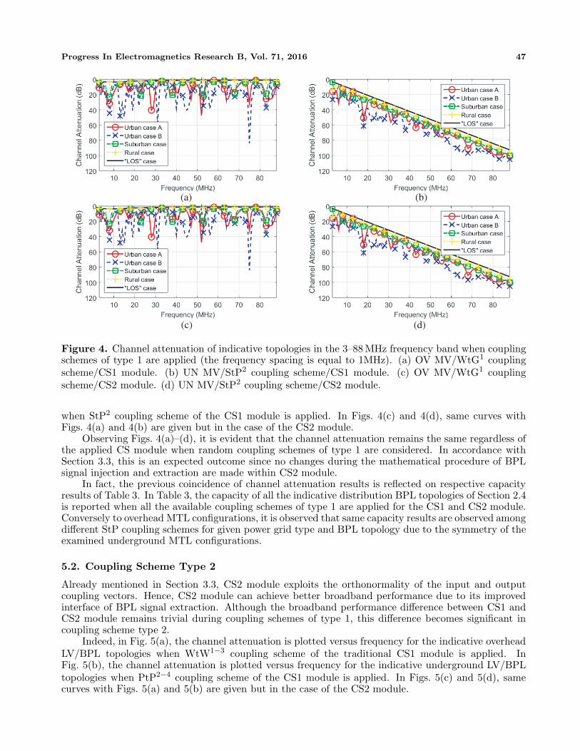
Progress In Electromagnetics Research B, Vol. 71, 2016 47

(a) (b)

(c) (d)

Figure 4. Channel attenuation of indicative topologies in the 3–88 MHz frequency band when couplingschemes of type 1 are applied (the frequency spacing is equal to 1MHz). (a) OV MV/WtG1 couplingscheme/CS1 module. (b) UN MV/StP2 coupling scheme/CS1 module. (c) OV MV/WtG1 couplingscheme/CS2 module. (d) UN MV/StP2 coupling scheme/CS2 module.

when StP2 coupling scheme of the CS1 module is applied. In Figs. 4(c) and 4(d), same curves withFigs. 4(a) and 4(b) are given but in the case of the CS2 module.

Observing Figs. 4(a)–(d), it is evident that the channel attenuation remains the same regardless ofthe applied CS module when random coupling schemes of type 1 are considered. In accordance withSection 3.3, this is an expected outcome since no changes during the mathematical procedure of BPLsignal injection and extraction are made within CS2 module.

In fact, the previous coincidence of channel attenuation results is reflected on respective capacityresults of Table 3. In Table 3, the capacity of all the indicative distribution BPL topologies of Section 2.4is reported when all the available coupling schemes of type 1 are applied for the CS1 and CS2 module.Conversely to overhead MTL configurations, it is observed that same capacity results are observed amongdifferent StP coupling schemes for given power grid type and BPL topology due to the symmetry of theexamined underground MTL configurations.

5.2. Coupling Scheme Type 2

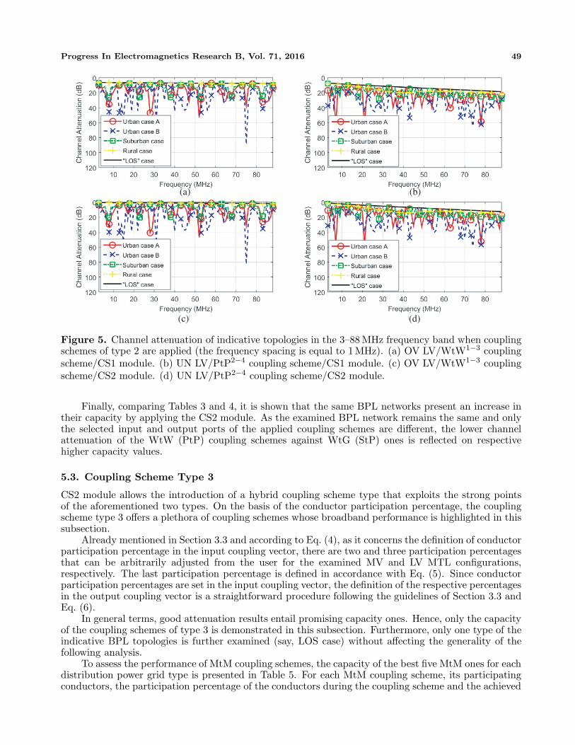
Already mentioned in Section 3.3, CS2 module exploits the orthonormality of the input and outputcoupling vectors. Hence, CS2 module can achieve better broadband performance due to its improvedinterface of BPL signal extraction. Although the broadband performance difference between CS1 andCS2 module remains trivial during coupling schemes of type 1, this difference becomes significant incoupling scheme type 2.

Indeed, in Fig. 5(a), the channel attenuation is plotted versus frequency for the indicative overheadLV/BPL topologies when WtW1−3 coupling scheme of the traditional CS1 module is applied. InFig. 5(b), the channel attenuation is plotted versus frequency for the indicative underground LV/BPLtopologies when PtP2−4 coupling scheme of the CS1 module is applied. In Figs. 5(c) and 5(d), samecurves with Figs. 5(a) and 5(b) are given but in the case of the CS2 module.

48 Lazaropoulos

Table 3. Capacity comparison of CS1 and CS2 module for different coupling schemes of type 1 (CS1module: blue/CS2 module: red and the frequency spacing is equal to 0.1 MHz).

Capacity (Mbps)

Power

Grid Type

Coupling

Schemes

MV

Urban Case A Urban Case B Suburban Case Rural Case “LOS” case

Overhead

WtG1 596/596 459/459 705/705 787/787 892/892

WtG2 599/599 462/462 709/709 790/790 896/896

WtG3 596/596 459/459 705/705 787/787 892/892

WtG4 - - - - -

Underground

StP1 815/815 685/685 890/890 968/968 1049/1049

StP2 815/815 685/685 890/890 968/968 1049/1049

StP3 815/815 685/685 890/890 968/968 1049/1049

StP4 - - - - -

LV

Overhead

WtG1 606/606 469/469 715/715 797/797 902/902

WtG2 608/608 471/471 717/717 799/799 904/904

WtG3 609/609 472/472 719/719 800/800 906/906

WtG4 606/606 470/470 716/716 798/798 903/903

Underground

StP1 1849/1849 1634/1634 1953/1953 2053/2053 2152/2152

StP2 1849/1849 1634/1634 1953/1953 2053/2053 2152/2152

StP3 1849/1849 1634/1634 1953/1953 2053/2053 2152/2152

StP4 1849/1849 1634/1634 1953/1953 2053/2053 2152/2152

From Figs. 5(a)–(d), it is obvious that CS2 module succeeds in reducing channel attenuation by6dB in all the cases examined. This improvement is due to the fact that CS1 module only permits theextraction of the one half of the BPL signal at the receiving end whereas the proposed output couplingvector of the CS2 module achieves to restore the entire BPL signal at the receiving end because of itsorthonormal elements.

The upgrade of the BPL signal extraction interface that is provided by the CS2 module alsoimproves the respective capacity results of coupling schemes of type 2. In Table 4, the capacity of allthe indicative distribution BPL topologies of Sec.IID is reported when all the available coupling schemesof type 2 are applied for the CS1 and CS2 module.

From Figs. 5(a)–(d) and Table 4, several interesting remarks regarding the operation of CS2 modulecan be deduced:

• The 6dB channel attenuation gain that is achieved by the BPL signal extraction interface of CS2module is translated into approximately 160 Mbps capacity gain. In fact, CS2 module rendersWtW/PtP coupling schemes almost equivalent to respective WtG/StP ones in terms of channelattenuation and capacity in all the BPL topologies examined.

• Similarly to the coupling schemes of type 1, due to the symmetry of distribution MTLconfigurations, comparable attenuation and capacity values are observed among different couplingschemes for given power grid type. Also, it should be noted that there is no attenuation and capacitydifference in coupling schemes of type 2 if the coupling configurations of the involved conductors areinverted (i.e., WtW1−2 and WtW2−1 coupling schemes present the same attenuation and capacityresults).

• In combination with their favourable characteristics concerning the reduced EMI to the otheralready existing communications services [12, 20], coupling schemes of type 2 are going to bequalified for the future’s BPL network deployment. Actually, the low EMI of coupling schemesof type 2 results from the differential excitation of the conductors, which blocks the propagation ofthe common mode across the BPL networks [1–7, 12–15, 20, 21, 26–29].

Progress In Electromagnetics Research B, Vol. 71, 2016 49

(a) (b)

(c) (d)

Figure 5. Channel attenuation of indicative topologies in the 3–88 MHz frequency band when couplingschemes of type 2 are applied (the frequency spacing is equal to 1MHz). (a) OV LV/WtW1−3 couplingscheme/CS1 module. (b) UN LV/PtP2−4 coupling scheme/CS1 module. (c) OV LV/WtW1−3 couplingscheme/CS2 module. (d) UN LV/PtP2−4 coupling scheme/CS2 module.

Finally, comparing Tables 3 and 4, it is shown that the same BPL networks present an increase intheir capacity by applying the CS2 module. As the examined BPL network remains the same and onlythe selected input and output ports of the applied coupling schemes are different, the lower channelattenuation of the WtW (PtP) coupling schemes against WtG (StP) ones is reflected on respectivehigher capacity values.

5.3. Coupling Scheme Type 3

CS2 module allows the introduction of a hybrid coupling scheme type that exploits the strong pointsof the aforementioned two types. On the basis of the conductor participation percentage, the couplingscheme type 3 offers a plethora of coupling schemes whose broadband performance is highlighted in thissubsection.

Already mentioned in Section 3.3 and according to Eq. (4), as it concerns the definition of conductorparticipation percentage in the input coupling vector, there are two and three participation percentagesthat can be arbitrarily adjusted from the user for the examined MV and LV MTL configurations,respectively. The last participation percentage is defined in accordance with Eq. (5). Since conductorparticipation percentages are set in the input coupling vector, the definition of the respective percentagesin the output coupling vector is a straightforward procedure following the guidelines of Section 3.3 andEq. (6).

In general terms, good attenuation results entail promising capacity ones. Hence, only the capacityof the coupling schemes of type 3 is demonstrated in this subsection. Furthermore, only one type of theindicative BPL topologies is further examined (say, LOS case) without affecting the generality of thefollowing analysis.

To assess the performance of MtM coupling schemes, the capacity of the best five MtM ones for eachdistribution power grid type is presented in Table 5. For each MtM coupling scheme, its participatingconductors, the participation percentage of the conductors during the coupling scheme and the achieved

50 Lazaropoulos

Table 4. Capacity comparison of CS1 and CS2 module for different coupling schemes of type 2 (CS1module: blue/CS2 module: red and the frequency spacing is equal to 0.1 MHz).

Capacity (Mbps)

Power

Grid Type

Coupling

Schemes

MV

Urban Case A Urban Case B Suburban Case Rural Case “LOS” case

Overhead

WtW1−2 463/612 346/476 562/722 638/803 739/909

WtW1−3 465/615 348/478 565/725 639/804 741/911

WtW1−4 - - - - -

WtW2−3 463/612 346/476 562/722 638/803 739/909

WtW2−4 - - - - -

WtW3−4 - - - - -

Underground

PtP1−2 698/815 581/685 767/890 838/968 913/1049

PtP1−3 698/815 581/685 767/890 838/968 913/1049

PtP1−4 - - - - -

PtP2−3 698/815 581/685 767/890 838/968 913/1049

PtP2−4 - - - - -

PtP3−4 - - - - -

LV

Overhead

WtW1−2 463/612 346/475 562/721 637/803 738/908

WtW1−3 467/616 349/479 566/726 642/807 743/912

WtW1−4 466/615 348/478 566/725 641/806 742/911

WtW2−3 463/612 346/475 561/721 637/803 738/908

WtW2−4 464/613 347/477 536/723 639/804 740/909

WtW3−4 460/609 343/472 558/718 634/800 735/904

Underground

PtP1−2 1634/1805 1420/1590 1739/1909 1838/2008 1938/2108

PtP1−3 1681/1851 1466/1636 1785/1955 1885/2055 1984/2154

PtP1−4 1635/1805 1420/1590 1739/1909 1838/2008 1937/2108

PtP2−3 1635/1805 1420/1590 1739/1909 1838/2008 1938/2108

PtP2−4 1681/1851 1466/1636 1785/1955 1885/2055 1984/2154

PtP3−4 1635/1805 1420/1590 1739/1909 1838/2008 1938/2108

capacity are analytically given.Comparing Tables 3–5, it is evident that the coupling schemes of type 3 may present better capacity

performance compared with the coupling schemes of type 1 and 2. In fact, the capacity increase mayreach up to 74 Mbps. This capacity surplus may become crucial when BPL networks aim at providingreliable communications during an emergency (emergency BPL communications network). Nevertheless,it should be examined whether this capacity surplus of MtM coupling schemes is worth the installationof the additional pairs of BPL signal injectors and extractors across the existing BPL networks.

In addition, the capacity increase of MtM coupling schemes is achieved by mainly using the groundand the shield of overhead and underground distribution BPL networks, respectively, rather thandifferential excitations. This fact comes from the nonzero algebraic sum of the conductor participationpercentage in the input coupling vector that implies a ground/shield return. But the use of either theground or the shield excites the common mode across the MTL configurations. Notorious for its presence,common mode is responsible for increasing the EMI of BPL networks to the other communicationsservices. Therefore, there is an interesting trade-off relation among capacity increase delivered by MtMcoupling schemes, installation cost of additional BPL injectors/extractors and EMI.

Finally, coupling scheme type 3 is a simple theoretical expansion of the CS2 module of twoconductors when three and four conductors are assumed without treating them as separate inputsand outputs like in MIMO systems. For the completeness of the theoretical analysis and comparisonreasons, the coupling scheme type 3 has also been presented. Although coupling scheme type 3 actsas the theoretical best case scenario of CS2 module, its return on investment (ROI) is regarded as

Progress In Electromagnetics Research B, Vol. 71, 2016 51

Table 5. Top 5 coupling schemes of type 3 for distribution BPL LOS cases when CS2 module is applied(The frequency spacing is equal to 0.1 MHz and the participation percentage step is equal to 0.1).

Capacity (Mbps)

Power

Grid Type

MV LV

Coupling Schemes“LOS”

caseCoupling Schemes

“LOS”

case

Overhead

MtM1−2−30.8 −0.1 −0.1 921 MtM1−2−3−4

0.7 −0.1 −0.1 −0.1 923

MtM1−2−3−0.1 −0.1 0.8 921 MtM1−3−4

0.8 −0.1 −0.1 921

MtM1−2−3−0.2 −0.1 0.7 918 MtM1−3−4

0.7 −0.2 −0.1 920

MtM1−2−3−0.1 0.8 −0.1 918 MtM1−2−3−4

0.6 −0.1 −0.1 −0.2 920

MtM1−2−30.7 −0.1 −0.2 918 MtM1−2−3−4

0.6 −0.1 −0.2 −0.1 920

Underground

MtM1−2−0.9 −0.1 1049 MtM1−2−4

−0.8 −0.1 −0.1 2228

MtM1−3−0.9 −0.1 1049 MtM1−2−3

−0.1 −0.8 −0.1 2228

MtM1−1 1049 MtM1−3−4

−0.1 −0.1 −0.8 2228

MtM1−3−0.9 0.1 1049 MtM1−2−3−4

−0.7 −0.1 0.1 −0.1 2203

MtM1−2−0.9 0.1 1049 MtM1−2−3−4

−0.1 −0.7 −0.1 0.1 2203

unacceptable in terms of the achieved capacity when MIMO and, more recently, massive MIMO can bedeployed [41, 46, 47].

5.4. Discussion about CS2 Module and Its Supported Coupling Schemes

CS2 module can drastically change the coupling scheme stereotypes in distribution BPL networks,namely:

(1) By adopting CS2 module, WtW and PtP coupling schemes become almost equivalent to respectiveWtG and StP coupling schemes in terms of channel attenuation and capacity. In combination withtheir low EMI, coupling schemes of type 2 are going to be the leading coupling scheme type duringthe future’s BPL network implementations.

(2) Since coupling schemes of low EMI will be deployed across the future’s BPL networks, newEMI policies with higher IPSD limits concerning the BPL operation will be established andmandated. Furthermore, the synthesis of new higher IPSD limits and multiple input multipleoutput (MIMO) technology features may metamorphose BPL networks into a multi-Gbps backhaulnetwork [41]. This multi-Gbps BPL network may support a myriad of smart grid applicationsincluding automated communication among components of the power grid, sensing, automatedcontrols for repairs, energy trading and improved decision support software [42–45].

(3) Contrary to CS1 module, CS2 module supports the new coupling scheme type 3 that may involveall the conductors of the MTL configuration. Although coupling scheme type 3 achieves thebest broadband performance metrics, there is a trade-off relation among the metric improvement,installation cost and EMI that needs further examination depending on the case scenario.

(4) Due to their tremendous capacity improvement, the deployment of MIMO schemes in distributionBPL networks, being well-known from the wireless world, is imperative in the following years.Hence, coupling schemes of type 3 may operate as the bridge between today’s and future’s BPLnetworks till appropriate EMI policies and network protocols are established.

6. CONCLUSIONS

This paper has focused on the broadband performance assessment of distribution BPL networks whenCS2 module is considered. Based on its new BPL signal coupling procedure of two interfaces, CS2module better exploits the existing conductors of the distribution MTL configurations as well as theinjected and extracted power of BPL signals.

52 Lazaropoulos

Synoptically, it has been shown that CS2 module maintains the same broadband performanceof coupling schemes of type 1 compared with CS1 module. As it concerns the coupling schemes oftype 2, CS2 module achieves to improve the channel attenuation and the capacity of distribution BPLnetworks on the basis of its advanced BPL signal extraction interface. In fact, the capacity increasemay reach up to 170Mbps when FCC Part 15 limits are considered in the 3–88 MHz frequency range.Compared with CS1 module, CS2 module introduces the coupling scheme type 3 that exploits all theavailable conductors of distribution MTL configurations. Although this type of coupling schemes mayoffer additional improvement of broadband performance metrics, there is a trade-off relation among themetric improvement, installation cost and EMI to other existing radioservices.

Finally, CS2 module renders coupling schemes of type 2 as the leading coupling trend. Due to theiralready known low-EMI features and the progress concerning their capacity, WtW and PtP couplingschemes are going to exclusively used during the design of the future’s BPL networks.

REFERENCES

1. Lazaropoulos, A. G., “Towards modal integration of overhead and underground low-voltageand medium-voltage power line communication channels in the smart grid landscape: Modelexpansion, broadband signal transmission characteristics, and statistical performance metrics(invited paper),” ISRN Signal Processing, Vol. 2012, Article ID 121628, 1–17, 2012. [Online].Available: http://www.hindawi.com/isrn/sp/2012/121628/.

2. Lazaropoulos, A. G., “Towards broadband over power lines systems integration: Transmissioncharacteristics of underground low-voltage distribution power lines,” Progress In ElectromagneticsResearch B, Vol. 39, 89–114, 2012.

3. Lazaropoulos, A. G. and P. G. Cottis, “Transmission characteristics of overhead medium voltagepower line communication channels,” IEEE Trans. Power Del., Vol. 24, No. 3, 1164–1173,Jul. 2009.

4. Lazaropoulos, A. G. and P. G. Cottis, “Capacity of overhead medium voltage power linecommunication channels,” IEEE Trans. Power Del., Vol. 25, No. 2, 723–733, Apr. 2010.

5. Lazaropoulos, A. G. and P. G. Cottis, “Broadband transmission via underground medium-voltagepower lines — Part I: Transmission characteristics,” IEEE Trans. Power Del., Vol. 25, No. 4,2414–2424, Oct. 2010.

6. Lazaropoulos, A. G. and P. G. Cottis, “Broadband transmission via underground medium-voltagepower lines — Part II: Capacity,” IEEE Trans. Power Del., Vol. 25, No. 4, 2425–2434, Oct. 2010.

7. Lazaropoulos, A. G., “Broadband transmission characteristics of overhead high-voltage power linecommunication channels,” Progress In Electromagnetics Research B, Vol. 36, 373–398, 2012.

8. Lazaropoulos, A. G., “Green overhead and underground multiple-input multiple-output mediumvoltage broadband over power lines networks: Energy-efficient power control,” Springer Journalof Global Optimization, Vol. 2012, 1–28, Oct. 2012, Print ISSN 0925-5001.

9. Ferreira, H., L. Lampe, J. Newbury, and T. G. Swart, Power Line Communications, Theoryand Applications for Narrowband and Broadband Communications over Power Lines, Wiley, NewYork, 2010.

10. Lazaropoulos, A. G., “Deployment concepts for overhead high voltage broadband over powerlines connections with two-hop repeater system: Capacity countermeasures against aggravatedtopologies and high noise environments,” Progress In Electromagnetics Research B, Vol. 44, 283–307, 2012.

11. Lazaropoulos, A. G., “Broadband transmission and statistical performance properties of overheadhigh-voltage transmission networks,” Hindawi Journal of Computer Networks and Commun.,article ID 875632, 2012. [Online]. Available: http://www.hindawi.com/journals/jcnc/aip/875632/

12. Amirshahi, P. and M. Kavehrad, “High-frequency characteristics of overhead multiconductorpower lines for broadband communications,” IEEE J. Sel. Areas Commun., Vol. 24, No. 7, 1292–1303, Jul. 2006.

Progress In Electromagnetics Research B, Vol. 71, 2016 53

13. Calliacoudas, T. and F. Issa, ““Multiconductor transmission lines and cables solver”, Anefficient simulation tool for PLC channel networks development,” IEEE Int. Conf. Power LineCommunications and Its Applications, Athens, Greece, Mar. 2002.

14. Sartenaer, T. and P. Delogne, “Deterministic modelling of the (Shielded) outdoor powerlinechannel based on the multiconductor transmission line equations,” IEEE J. Sel. Areas Commun.,Vol. 24, No. 7, 1277–1291, Jul. 2006.

15. Paul, C. R., Analysis of Multiconductor Transmission Lines, Wiley, New York, 1994.16. Meng, H., S. Chen, Y. L. Guan, C. L. Law, P. L. So, E. Gunawan, and T. T. Lie, “Modeling

of transfer characteristics for the broadband power line communication channel,” IEEE Trans.Power Del., Vol. 19, No. 3, 1057–1064, Jul. 2004.

17. Li, B., D. Mansson, and G. Yang, “An efficient method for solving frequency responses of power-line networks,” Progress In Electromagnetics Research B, Vol. 62, 303–317, 2015.

18. Chaaban, M., K. El Khamlichi Drissi, and D. Poljak, “Analytical model for electromagneticradiation by bare-wire structures,” Progress In Electromagnetics Research B, Vol. 45, 395–413,2012.

19. Kim, Y. H., S. Choi, S. C. Kim, and J. H. Lee, “Capacity of OFDM two-hop relaying systems formedium-voltage power-line access networks,” IEEE Trans. Power Del., Vol. 27, No. 2, 886–894,Apr. 2012.

20. Amirshahi, P. and M. Kavehrad, “Medium voltage overhead powerline broadband communica-tions; Transmission capacity and electromagnetic interference,” Proc. IEEE Int. Symp. PowerLine Commun. Appl., 2–6, Vancouver, BC, Canada, Apr. 2005.

21. OPERA1, D44: Report presenting the architecture of plc system, the electricity networktopologies, the operating modes and the equipment over which PLC access system will be installed,IST Integr. Project No 507667, Dec. 2005.

22. OPERA1, D5: Pathloss as a function of frequency, distance and network topology for various LVand MV European powerline networks. IST Integrated Project No 507667, Apr. 2005.

23. Veen, J., P. C. J. M. van der Wielen, and E. F. Steennis, “Propagation characteristics of three-phase belted paper cable for on-line PD detection,” Proc. 2002 IEEE International Symposiumon Electrical Insulation, ELINSL02, 96–99, Boston, MA, USA, Apr. 2002.

24. Van der Wielen, P. C. J. M., E. F. Steennis, and P. A. A. F. Wouters, “Fundamental aspectsof excitation and propagation of on-line partial discharge signals in three-phase medium voltagecable systems,” IEEE Trans. Dielectr. Electr. Insul., Vol. 10, No. 4, 678–688, Aug. 2003.

25. Tang, M. and M. Zhai, “Research of transmission parameters of four-conductor cables for powerline communication,” Proc. Int. Conf. on Computer Science and Software Engineering, Vol. 5,1306–1309, Wuhan, China, Dec. 2008.

26. Issa, F., D. Chaffanjon, E. P. de la Bathie, and A. Pacaud, “An efficient tool for modal analysistransmission lines for PLC networks development,” IEEE Int. Conf. Power Line Communicationsand Its Applications, Athens, Greece, Mar. 2002.

27. D’Amore, M. and M. S. Sarto, “A new formulation of lossy ground return parameters for transientanalysis of multiconductor dissipative lines,” IEEE Trans. Power Del., Vol. 12, No. 1, 303–314,Jan. 1997.

28. D’Amore, M. and M. S. Sarto, “Simulation models of a dissipative transmission line above alossy ground for a wide-frequency range — Part I: Single conductor configuration,” IEEE Trans.Electromagn. Compat., Vol. 38, No. 2, 127–138, May 1996.

29. D’Amore, M. and M. S. Sarto, “Simulation models of a dissipative transmission line above alossy ground for a wide-frequency range — Part II: Multi-conductor configuration,” IEEE Trans.Electromagn. Compat., Vol. 38, No. 2, 139–149, May 1996.

30. Anatory, J., N. Theethayi, R. Thottappillil, M. M. Kissaka, and N. H. Mvungi, “The influenceof load impedance, line length, and branches on underground cable power-line communications(PLC) systems,” IEEE Trans. Power Del., Vol. 23, No. 1, 180–187, Jan. 2008.

54 Lazaropoulos

31. Lazaropoulos, A. G., “Factors influencing broadband transmission characteristics of undergroundlow-voltage distribution networks,” IET Commun., Vol. 6, No. 17, 2886–2893, Nov. 2012.

32. Anatory, J., N. Theethayi, and R. Thottappillil, “Power-line communication channel model forinterconnected networks — Part II: Multiconductor system,” IEEE Trans. Power Del., Vol. 24,No. 1, 124–128, Jan. 2009.

33. Anatory, J., N. Theethayi, R. Thottappillil, M. M. Kissaka, and N. H. Mvungi, “The effects ofload impedance, line length, and branches in typical low-voltage channels of the BPLC systemsof developing countries: Transmission-line analyses,” IEEE Trans. Power Del., Vol. 24, No. 2,621–629, Apr. 2009.

34. Gebhardt, M., F. Weinmann, and K. Dostert, “Physical and regulatory constraints forcommunication over the power supply grid,” IEEE Commun. Mag., Vol. 41, No. 5, 84–90,May 2003.

35. Henry, P. S., “Interference characteristics of broadband power line communication systems usingaerial medium voltage wires,” IEEE Commun. Mag., Vol. 43, No. 4, 92–98, Apr. 2005.

36. Ofcom, “Amperion PLT Measurements in Crieff,” Ofcom, Tech. Rep., Sept. 2005.37. NATO, “HF Interference, Procedures and Tools (Interferences HF, procedures et outils) Final

Report of NATO RTO Information Systems Technology,” RTO-TR-ISTR-050, Jun. 2007, [On-line]. Available: http://ftp.rta.nato.int/public/PubFullText/RTO/TR/RTO-TR-IST-050/TR-IST-050-ALL.pdf

38. FCC, “In the Matter of Amendment of Part 15 regarding new requirements and measurementguidelines for Access Broadband over Power Line Systems,” FCC 04-245 Report and Order,Jul. 2008.

39. Ofcom, “DS2 PLT Measurements in Crieff,” Ofcom, Tech. Rep. 793 (Part 2), May 2005.40. Ofcom, “Ascom PLT Measurements in Winchester,” Ofcom, Tech. Rep. 793 (Part 1), May 2005.41. Lazaropoulos, A. G., “Broadband over Power Lines (BPL) systems convergence:

Multiple-Input Multiple-Output (MIMO) communications analysis of overhead andunderground low-voltage and medium-voltage BPL networks (invited paper),” ISRNPower Engineering, Vol. 2013, Article ID 517940, 1–30, 2013. [Online]. Available:http://www.hindawi.com/isrn/power.engineering/2013/517940/.

42. El Haj, Y., L. Albasha, A. El-Hag, and H. Mir, “Data communication through distributionnetworks for smart grid applications,” IET Science, Measurement & Technology, Vol. 9, No. 6,774–781, 2015.

43. Lazaropoulos, A. G., “Wireless sensor network design for transmission line monitoring, meteringand controlling: Introducing Broadband over PowerLines-enhanced Network Model (BPLeNM),”ISRN Power Engineering, Vol. 2014, Article ID 894628, 22 pages, 2014, doi:10.1155/2014/894628.[Online]. Available: http://www.hindawi.com/journals/isrn.power.engineering/2014/894628/.

44. Lazaropoulos, A. G., “Wireless sensors and broadband over powerlines networks: The performanceof Broadband over PowerLines-enhanced Network Model (BPLeNM) (invited paper),” ICASPublishing Group Transaction on IoT and Cloud Computing, Vol. 2, No. 3, 1–35, 2014. [Online].Available: http://icas-pub.org/ojs/index.php/ticc/article/view/27/17.

45. Lazaropoulos, A. G. and P. Lazaropoulos, “Financially stimulating local economies byexploiting communities’ microgrids: Power trading and Hybrid Techno-Economic (HTE)model,” Trends in Renewable Energy, Vol. 1, No. 3, 131–184, Sept. 2015. [Online]. Available:http://futureenergysp.com/index.php/tre/article/view/14.

46. Lazaropoulos, A. G., “Overhead and underground MIMO low voltage broadband over power linesnetworks and EMI regulations: Towards greener capacity performances,” Elsevier Computers andElectrical Engineering, Vol. 39, 2214–2230, 2013.

47. Lazaropoulos, A. G., “Policies for carbon energy footprint reduction of overheadmultiple-input multiple-output high voltage broadband over power lines networks,”Trends in Renewable Energy, Vol. 1, No. 2, 87–118, Jun. 2015. [Online]. Available:http://futureenergysp.com/index.php/tre/article/view/11/17.