BACHELOR THESIS 15 CREDITSDEPARTMENT OF GEOPHYSICS

New concept for monitoring SO2 emissionsfrom Tavurvur volcano in Papua New Guinea

Author:Julia WALLIUS

Supervisor:Prof. Olafur GUDMUNDSSON

A thesis submitted in fulfillment of the requirementsfor the degree of Bachelor

in

Physics

December 22, 2017

Sammanfattning

Nytt koncept för att övervaka SO2 utsläpp från vulkanen Tavurvur i Papua NyaGuineaJulia Wallius

Under en period på 29 dagar under oktober månad 2016 kördes ett dubbelstrålatDOAS instrument med brett synfält på ön Matupit i Papua Nya Guinea. Detta för attmäta svaveldioxidutsläppen från vulkanen Tavurvur, som ligger på Gazelle halvön iprovinsen East New Britain. På grund av otillförlitliga inställningar under de första 17dagarna så utgick de slutgiltliga resultaten från mätningar tagna mellan den 19:e och30:e oktober med ett två dagars uppehåll under den 25:e och 26:e oktober då instru-mentet användes för att istället erhålla vindhastighetdata. Det genomsnittliga flödet avSO2 bestämmdes för denna period till att ligga på 0.27 kg

smed en vindhastighet på

3.9 ms

. Användandet av ett dubbelstrålat DOAS instrument med brett synfält rekom-menderas vid Tavurvur när gasutsläppen är låga och vindriktningen är övervägandesydvästlig. En vinkel på 13 grader över horisonten användes för att erhålla refer-ensspektra av himlen för varje skanningsuppsättning men på grund av SO2 spår i dessaspektra så anses denna vinkel vara för liten och att höja denna mellan 5-10 grader förreferensspektra rekommenderas för framtida mätningar.

Nyckelord: Optisk fjärranalys, DOAS, Vulkanövervakning, SO2-utsläpp

Examensarbete C i geofysik, 1GE037, 15 hp, 2017Handledare: Olafur GudmundssonInstitutionen för geovetenskaper, Uppsala universitet, Villavägen 16, 752 36 Uppsala(www.geo.uu.se)

Hela publikationen finns tillgänglig på www.diva-portal.org

Abstract

New concept for monitoring SO2 emissions from Tavurvur volcano in Papua NewGuineaJulia Wallius

During a period of 29 consecutive days during the month of October 2016 a dual-beam wide-field-of-view DOAS instrument was deployed at Matupit Island in PapuaNew Guinea. This was to measure the sulphur dioxide emissions from Tavurvur vol-cano located on the Gazelle Peninsula of the island East New Britain. Due to unreliablesettings for the first 17 days the final results used were derived from measurementstaken between October 19th and 30th with a two day gap during the 25th and 26th ofOctober when the instrument was used for obtaining wind speed data. The average

i

flux of SO2 was determined for the period to be 0.27 kgs

with a wind speed estimation of3.9 m

s. The use of a dual-beam wide-field-of-view DOAS instrument is recommended at

Tavurvur when the degassing levels are low and the wind is predominantly southwest-erly. An angle of 13 degrees above the horizon was used to obtain the sky referencespectrum for each set of scans, but on account of SO2 traces in these spectra this an-gle is considered too low and lifting the sky reference 5-10 degrees is recommendedfor future measurements.

Keywords: Optic remote sensing, DOAS, Volcano monitoring, SO2 emissions

Independent Degree Project C in Geophysics, 1GE037, 15 credits, 2017Supervisor: Olafur GudmundssonDepartment of Earth Sciences, Uppsala University, Villavägen 16, SE-752 36Uppsala (www.geo.uu.se)

The whole document is available at www.diva-portal.org

ii

AcknowledgementsThis project would not have been possible without the invaluable help from Rabaul Vol-canological Observatory, in particular Kila Mulina and Ima Itikarai. Special thanks alsogo out to John Bosco and Ezequiel from RVO for their work assembling and installingthe instrument on site. And finally, a huge thank you to Bo Galle and Santiago Arel-lano from Chalmers University for allowing me to be a part of their Papua New Guineafield campaign and all the help and support they provided both on site and before de-parture. Funding for this project was provided by a SIDA Minor Field Study grant andDCO-DECADE.

iii

A note on the text

As part of the larger Rabaul caldera Tavurvur in itself is not a volcano but merely asub-vent. However, for simplification, Tavurvur is referred to as a volcano throughoutthis thesis.

iv

Contents

Acknowledgements iii

List of Abbreviations vii

1 Introduction 11.1 Rabaul caldera . . . . . . . . . . . . . . . . . . . . . . . . . . . . . . . . 11.2 Method and purpose of study . . . . . . . . . . . . . . . . . . . . . . . . 2

2 Background 52.1 Differential Optical Absorption Spectroscopy . . . . . . . . . . . . . . . . 5

2.1.1 Lambert-Beer’s Law . . . . . . . . . . . . . . . . . . . . . . . . . 62.2 DOAS Measurements and Corrections . . . . . . . . . . . . . . . . . . . 7

2.2.1 Fraunhofer spectrum . . . . . . . . . . . . . . . . . . . . . . . . . 82.2.2 Ring effect . . . . . . . . . . . . . . . . . . . . . . . . . . . . . . 82.2.3 High-pass filtering . . . . . . . . . . . . . . . . . . . . . . . . . . 92.2.4 Dark current . . . . . . . . . . . . . . . . . . . . . . . . . . . . . 92.2.5 Sky reference . . . . . . . . . . . . . . . . . . . . . . . . . . . . . 9

2.3 Dual-beam wide-field-of-view DOAS . . . . . . . . . . . . . . . . . . . . 92.4 Elevation angle . . . . . . . . . . . . . . . . . . . . . . . . . . . . . . . . 112.5 Wind speed calculation . . . . . . . . . . . . . . . . . . . . . . . . . . . 122.6 Previous DOAS measurements on Tavurvur . . . . . . . . . . . . . . . . 12

3 Method 133.1 Materials and instrument assembling . . . . . . . . . . . . . . . . . . . . 133.2 Configuration and testing of instrument . . . . . . . . . . . . . . . . . . . 153.3 Installation . . . . . . . . . . . . . . . . . . . . . . . . . . . . . . . . . . 153.4 Scanner settings and properties . . . . . . . . . . . . . . . . . . . . . . 16

3.4.1 Measurement modes . . . . . . . . . . . . . . . . . . . . . . . . 16Sensitive detection . . . . . . . . . . . . . . . . . . . . . . . . . . 16Average flux . . . . . . . . . . . . . . . . . . . . . . . . . . . . . 16

3.5 Data evaluation . . . . . . . . . . . . . . . . . . . . . . . . . . . . . . . . 19

4 Results 214.1 Offsets . . . . . . . . . . . . . . . . . . . . . . . . . . . . . . . . . . . . . 214.2 SO2 fluxes . . . . . . . . . . . . . . . . . . . . . . . . . . . . . . . . . . 23

v

5 Discussion 255.1 Wind direction and speed . . . . . . . . . . . . . . . . . . . . . . . . . . 255.2 Recommendation . . . . . . . . . . . . . . . . . . . . . . . . . . . . . . . 25

6 Conclusions 26

Bibliography 27

vi

List of Abbreviations

COSPEC Correlation SpectroscopyD DayDB-WFOV Dual-beam wide-field-of-viewDCO-DECADE Deep Carbon Observatory, Deep Earth Carbon DegassingDECADE Deep Earth Carbon DegassingDOAS Differential Optical Absorption SpectroscopyGPS Global Positioning SystemKG KilogramM MeterNOVAC Network for Observation of Volcanic and Atmospheric ChangeO3 OzonePPM Parts Per MillionRVO Rabaul Volcanological ObservatoryS SecondSO2 Sulphur dioxideT TonUV Ultraviolet

vii

Chapter 1

Introduction

For many years, volcanological monitoring has been an important tool used in order tofurther our understanding of the workings of volcanoes and the degree to which we canaccurately predict a coming volcanic eruption (United States Geological Survey 2016).To this end, scientists have long recognized that the surveillance of volcanic gases playan important part, as gases dissolved in magma provide the driving force of volcaniceruptions. The observation of any changes in the release of certain gases from a vol-cano can therefore help forecast volcanic activity and provide insight into the processesbehind eruptions (United States Geological Survey 2015). More specifically, the be-havior of magma bodies as they ascent and descent in relation to eruptions can bebetter understood by conducting high temporal SO2 emission measurements over longtime periods (Galle et al., 2010). Together with other geophysical data it is also possi-ble to interpret the relationship between magma ascent and conduit and hydrothermalprocesses (Olmos et al., 2007) (Sparks, 2003). In fact, the relationship between gassignals and other geophysical measurement methods is conceivably strong, and it ispossible that the process of volcanic degassing is responsible for, or at least closelyrelated to, observed ground deformation and seismicity (Oppenheimer and McGonigle,2004).

Volcanoes also contribute to the release of many toxic gases into the atmosphere,which makes them a relevant study in context with the Earth’s climate. During recentyears this specific topic has been given more and more attention, as the emission ofa wide variety of volatile species, some of which are converted into aerosols duringtransport in the atmosphere, makes volcanism one of the main climate-forcing agentsand a natural volatile source with important impact upon ecosystems at both local andregional scales (Allard et al., 2016). By measuring the gas emissions, evaluating thedata and observing any underlying trends, the potential impact of volcanic emissionson the atmosphere and climate can begin to be understood.

1.1 Rabaul caldera

Papua New Guinea occupies the eastern half of the island of New Guinea and itsoffshore islands in Melanesia, placing it in the pacific “Ring of fire” - a name givento the ring of volcanoes around the Pacific Ocean, a result of plate tectonics - whichmakes it highly prone to disaster.

1

Chapter 1. Introduction

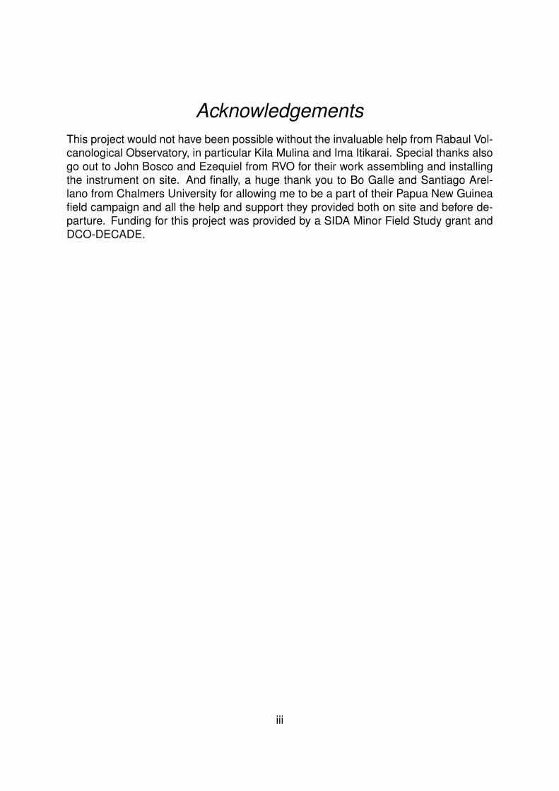
At the northeastern end of the province East New Britain lies Rabaul, a small towninside a large caldera known as Rabaul Volcano. For many years Rabaul was consid-ered the most important settlement of the province and served as a popular boatingdestination for both commercial and recreational purposes (Wikipedia 2017), beforethe eruptions of the sub-vents Tavurvur and Vulcan in 1994 devastated the town.

The present-day shape of the caldera, with a wide opening where the sea formsBlanche Bay to the east, is reckoned to have been formed by a major eruption around1400 years ago (Volcano Discovery 2017). Besides Tavurvur and Vulcan, other ventsalong its 14 km length include Turanguna, Rabalanakia, Sulphur Creek, Kombiu andthe Beehives.

The Rabual Volcanological Observatory (RVO) is a branch of the Geological Surveyof Papua New Guinea and monitors 37 volcanoes (World Organization of Volcano Ob-servatories 2015) spread out through Papua New Guinea. It was formed in 1937, afterVulcan and Tavurvur erupted and killed 507 people (Wikipedia 2017). When Vulcanand Tavurvur had their next eruptions in 1994, the people of Rabaul were better pre-pared by having planned for such an event, and only five people were killed. However,the huge amounts of ash sent into the air during the eruptions caused 80 percent of thebuildings of the town to collapse, and Rabual was completely devastated. This causedthe province’s capital, along with a major part of the population, to move from Rabaulto the nearby town Kokopo.

Papua New Guinea is considered one of the most significant sources of volcanicdegassing in the world (UN World Conference on Disaster Risk and Reduction 2015).After the eruptions in 1994, the most closely monitored volcano, Tavurvur, was identi-fied by Andreas and Kasgnoc (1998) as a sporadic emitter and capable of an outputof 301 kg

sof SO2 during eruptive periods (Andres and Kasgnoc, 1998) for the years

1973-1998. More recently, RVO conducted measurements of the volcano for the pe-riod 2009-2014 and found an estimated 3 kg

sof SO2, using a measurement method

of traverses with a portable FLYSPEC system (Horton et al., 2006). From the experi-ence gained during the eruptions of Tavurvur between 1994 and 2014, the emission ofSO2 has been regarded as an important indicator of precursory eruptive activity for thisvolcano (Mulina, 2015)

1.2 Method and purpose of study

In this study a stationary Differential Optical Absorption Spectroscopy (DOAS) instru-ment has been used to measure the SO2 emissions from Tavurvur volcano during aperiod of approximately four weeks. A DOAS instrument is a remote sensor whichmeasures the amount of skylight UV radiation that is absorbed by the volcanic gas,and determines the concentration of the gas by measuring its specific narrow bandabsorption structures in the UV and visible spectral region (Platt and Perner, 1983a).The study was conducted in order to better understand the workings of Tavurvur andto therefore be able to better foresee a coming eruption, as well as potential changesin the volcano’s behavior.

2

Chapter 1. Introduction

Upon arriving at Tavurvur and doing some initial DOAS measurements, it was con-cluded that the gas emissions were too low to accurately measure by standard scansand transects from a point below the gas puffs (Arellano, Galle, and Wallius, 2017a).Therefore an alternative concept for the measurements was proposed, where onewould observe the emissions at a fixed position close to the point of emission. In thisproject the purpose has been to determine if such an approach to SO2 emission mea-surements at Tavurvur yield dependable results. If so, they might be a viable alternativeto standard DOAS scans when the emission rates are low.

3

Chapter 1. Introduction

FIGURE 1.1: Overview of Rabaul Volcano (Wunderman, 1994). Activevents are marked with black dots and extinct cones with white dots. RVO

is represented by a black square.

4

Chapter 2

Background

The sensing method used in this study is based on spectroscopic observation of molec-ular species, in this case SO2. By observing their specific electronic, vibrational androtational transitions as recognized in the process of absorption, specific gases aredetectable(Oppenheimer and McGonigle, 2004). In the context of volcano monitoring,a combination of traverses or scans of volcanic clouds using a spectroscopy basedsensing method and the measurement of plume transport speed can determine fluxesof different gases (Galle, 2003)(Oppenheimer and McGonigle, 2004).

DOAS is a recognized technique used for the monitoring of SO2 emissions fromvolcanoes in order to obtain gas fluxes from active volcanoes around the world, asverified by the project NOVAC (Network for Observation of Volcanic and AtmosphericChange) which utilizes DOAS instruments in a global network of stations for the quan-titative measurement of volcanic gas emissions (Galle et al., 2010)(NOVAC Project2017). The DOAS instrument, in particular the mini-DOAS, is thanks to its size andweight relatively easy to carry up to a volcanic crater or to carry around the base of avolcano making it an attractive alternative to other remote sensing techniques such asfor example COSPEC (Correlation Spectroscopy) (Humaida, 2010).

2.1 Differential Optical Absorption Spectroscopy

The following section on Differential Optical Absorption Spectroscopy is largely basedon Stefan Kraus Ph.D dissertation on DOAS (Kraus, 2006) and Samuel Brohedes pa-per on the same subject (Brohede, 2002).

Differential Optical Absorption Spectroscopy is a method used to measure atmo-spheric trace gases in the atmosphere. It is based on absorption spectroscopy in theUV and visible wavelength range and makes use of either an artificial light source orsunlight that has passed through a specific volume of gas; a simple set up can besunlight passing through a gas cell containing SO2 measured by a single spectrome-ter at a given spectral wavelength range. Use of the DOAS measurement techniqueallows the separation of the absorption structures of several atmospheric species fromeach other as well as from the extinction due to scattering on molecules and aerosols,since it is based on the measurement of absorption spectra as opposed to the in-tensity of monochromatic light (light of one strictly constant and specific frequency).Platt provides an in-depth description of DOAS (Platt, 1994) and together with Perner

5

Chapter 2. Background

introduced the method (Platt and Perner, 1983b). To accurately obtain the desiredinformation, for example the concentration of gas species within a certain volume ofgas, it is necessary to understand the absorption behavior, i.e. the impacts of matterto electro-magnetical rays and how the species change the light that goes through it.To understand this, it is necessary to take a look at Lambert-Beer’s Law.

2.1.1 Lambert-Beer’s Law

Lambert-Beer’s Law defines how a layer of different substances will diminish the in-tensity of light at a specific wavelength. Equation 2.1 describes how the absorptionstructure looks like:

I(λ) = I0(λ)e−σ(λ)·L·n (2.1)

I(λ) is the measured intensity while I0(λ) represents the source intensity, both atgiven wavelengths. I0 is absorbed according to the substance’s number density n(molecules per cm3) along a path of light L. The so called cross-section σ(λ) gives thewavelength dependent absorption strength of the substance and describes the lightabsorption at a specific wavelength λ.

For later evaluations it is important to know the cross-section as precisely as possi-ble; different substances have different specific cross-sections. These can, for exam-ple, be obtained from lab measurements or literature data.

The dimensionless quantity σ(λ) ·L · n is often referred to as the Optical Depth andhere represented by τ .

When measuring light observed through the atmosphere different scattering pro-cesses also contribute to the radiation extinction. Though not technically absorptionprocesses, Rayleigh and Mie scattering behaves in a similar way by scattering lightaway from the line of vision. Adding this scattering to equation 1 results in the follow-ing:

τ(λ) = lnI0(λ)

I(λ)= L(σ(λ) · n+ εR(λ) + εM(λ)) (2.2)

The product of the Rayleigh cross-section and the number density nair for air cre-ates the Rayleigh extinction coefficient εR(λ). The Mie extinction coefficient εM(λ) issimilarly made up of the Mie cross-section multiplied by nair.

To include all atmospheric species with significant absorption cross-sections in thespecified wavelength the Lambert-Beer’s law is extended. If the atmosphere is opticallythin, i.e. if τ is much smaller than 1, then the additional species i can simply be added:

τ(λ) = L(∑i

(σi(λ) · ni + εR(λ) + εM(λ)))A(λ) (2.3)

6

Chapter 2. Background

In the equation above an additional function has also been added, A(λ), whichdescribes the attenuation of the instrument optics.

The cross-sections σi can be separated into two parts, as seen in equation 2.4, de-pending on their variation: σsi (λ) varies slowly with wavelength and σ′i(λ) varies rapidlywith wavelength. This latter, rapidly varying, part is also known as the differential cross-section.

σi(λ) = σsi (λ) + σ′i(λ) (2.4)

Rayleigh and Mie scattering, and the attenuation factor A(λ) are all slowly varyingwith wavelength and can therefore be expressed as a slowly varying part of the opticaldepth τ . Combining equation 2.4 with 2.3 gives:

τ(λ) = L∑i

σ′i(λ) · ni︸ ︷︷ ︸rapid, τ ′

+L(∑i

(σsi (λ) · ai + εR(λ) + εM(λ)))A(λ)︸ ︷︷ ︸slow, τs

(2.5)

By pairing the rapidly varying part τ ′(λ) of the measured optical depth to the ab-sorption resulting from the differential cross-sections, a separation of the slowly andrapidly varying optical depth is possible. Rayleigh and Mie scattering can together withthe attenuation factor now be disregarded by only studying differential cross-sectionsand the rapidly varying part of the optical depth:

τ ′(λ) = lnI ′0(λ)

I(λ)= L

∑i

σ′i(λ) · ni (2.6)

Equation 2.1 is dependent on the knowledge of the original light source intensityI0 which, in real-life measurements using the sun as light source, can be very difficultto establish as it includes simulating an atmosphere free of absorption. When usingDOAS instruments only the differential optical depth is important which includes themuch simpler task of instead simulating an atmosphere free of differential absorption.

Figure 2.1 shows the relationship between Optical Depth, Differential Optical Depth,light source intensity, and measured light intensity.

2.2 DOAS Measurements and Corrections

In this study measurements were done using stray light with the sun as light source,something known as "passive" measurements since it does not make use of an arti-ficial light source. When doing stray light measurements, as opposed to direct lightmeasurements using an artificial light, only light scattered due to Mie- and Rayleighscattering is recorded. When the size of a scatterer is much smaller than the wave-length of the incident electromagnetic radiation, Rayleigh scattering takes place. Ifhowever the size of the scatterer is much larger than the wavelength of the incident

7

Chapter 2. Background

FIGURE 2.1: The logarithm of the fraction between the light source inten-sity I0(λ) and the measured light intensity I(λ) describes Optical Depthτ(λ). The fraction between the interpolated source intensity I ∗ (λ) andthe measured intensity I(λ) describes the Differential Optical Depth τ ′(λ).

electromagnetic radiation, then Mie scattering occurs. Rayleigh scattering is what pro-duces the blue light of the sky, while Mie scattering gives the sun a white glare, and fogand mist a white light.

In order for the final spectra to be reliable, a number of different corrections mustbe applied to the light collected with the telescope and spectrometer. The ones usedin this study are listed and briefly explained below.

2.2.1 Fraunhofer spectrum

When using the sun as a light source a correction known as Fraunhofer must be appliedto the spectrum. This is due to the fact that the sun’s photosphere absorbs a part ofthe light emitted by itself, so absorption structures will already exist even if there is noatmosphere in the light path. The Fraunhofer correction is evaluated while recording aspectrum looking directly into the sun. This is then applied as a cross-section referenceduring evaluation of subsequent spectral measurements.

2.2.2 Ring effect

The Fraunhofer spectrum does not suffice to correct the measured spectra. Becauseof so called Raman scattering in the atmosphere (Lampel, Friess, and Platt, 2015)the Fraunhofer absorption lines get ’filled up’. This is known as a Ring effect. A Ringspectrum is calculated based on the Fraunhofer spectrum in order to correct for it. The

8

Chapter 2. Background

Ring-corrected Fraunhofer correction is used as yet another reference spectrum duringevaluation.

2.2.3 High-pass filtering

To remove all the low frequency parts of the spectrum that are not required for evalua-tion a high-pass filter it applied. This removal is desirable since the procedure behindthe DOAS method depends on the separation of the measured data into two parts:high frequency and low frequency data (see section 2.1).

2.2.4 Dark current

A current, known as the dark current, is generated within the instrument even whenthe spectrometer is not illuminated. This current changes based on the temperatureof the instrument, but as the power budget for most stations is limited, regulating thistemperature is not possible and all spectra must be corrected for this offset in the pro-cessing stage. To do this, no light is permitted to enter the spectrometer during onesingle spectral measurement and taken to represent the dark current. All the subse-quent spectra collected within a limited time span will be assumed to have the samedark current, which is then subtracted from every spectrum before further processing.

2.2.5 Sky reference

Another necessary correction to enhance the sensitivity to volcanic SO2 emissions con-sists of removing the effect of the background atmosphere. This is done by measuringa spectrum outside of the plume, called the "sky spectra" or "sky reference", which allthe subsequent plume spectra are divided by to reduce this background "noise" madeup mostly of spectral lines originating from H2O and CO2 and molecular scattering ofshorter wavelengths.

2.3 Dual-beam wide-field-of-view DOAS

The DOAS instrument used for this study is an alternative to the standard, single-beamnarrow-field-of-view telescope DOAS. Instead, it makes use of a dual-beam UV spec-trometer equipped with a wide-field-of-view telescope (hereafter known by the acronymDB-WFOV) that gathers light instantaneously from two narrow, spatially separated re-gions of the volcanic gas plume (Boichu et al., 2004). As two sections of the plumeare measured at the same instant, with a small angle separating the fields-of-view, thetime-series of the measured gas regions can be cross-correlated to retrieve the trans-port speed of the plume through time, though this will require additional informationconcerning the viewing and plume geometry (Boichu et al., 2004). If such informationis available, such a type of system is able to measure volcanic gas fluxes with bothhigh accuracy and high time resolution.

9

Chapter 2. Background

When having this setup with a wide-field-of-view, the telescope will "see" in thesame scene both regions with high and low concentrations of gas. The radiation theinstrument receives will be the sum of radiation from these low and high concentrationregions. Since each of these regions are subject to the absorption law, which is ex-ponentially dependent on the concentration, the total signal will come from the sum ofexponential terms, which are non-linear. This is not equivalent to having a single expo-nential of the concentrations of the different regions. If all regions instead have a lowgas concentration, the absorption law exponential is expanded in a polynomial and onlythe first term is important. This means that the absorption of different sectors dependlinearly on the concentration. The sum of the signals is then equivalent to the sum ofconcentrations. If the emission of SO2 is large, the concentration will normally be highin some regions and low in others, which would make this WFOV method inaccurate.But for the low emission situation at Tavurvur, it may prove ideal.

FIGURE 2.2: Sketch of the principle of measurement by a DB-WFOVscanning-DOAS instrument.

10

Chapter 2. Background

2.4 Elevation angle

It is important to determine a correct elevation angle for the scanner. This is to ensurethat the scanner measures the plume against a clear-sky background. An elevationangle that is too high can result in the scanner only observing clear sky, not samplingthe plume at all, while an elevation angle that is too low might result in the scannerbeing blocked by a mountain or other obstacle and not receiving enough light frombehind the plume.

To optimize the elevation angle of the scanner the intensity of radiation in the twospectrometer channels needs to be observed as a function of elevation and azimuthangles. The geometry involved in calculating the angle is shown in figure 2.3 below.

FIGURE 2.3: Sketch of elevation angle calculation. The box on the leftrepresents the scanner while the box on the right represents the highest

obstacle in the viewing direction of the telescope.

The box on the left represents the scanner and the box on the right represents theposition of the highest obstacle in the viewing direction of the scanner telescope. ∆Lis the distance between the two while ∆h is the difference in elevation of the boxes.Θ denotes the elevation angle above the horizontal and ∆ω the field of view of thetelescope. These parameters give an equation as follows:

Θ = atan(∆h+ (1

2)√

∆h2 + ∆L2∆ω

∆L) (2.7)

When all the parameters on the right-hand side are known, the elevation angle canbe determined.

11

Chapter 2. Background

2.5 Wind speed calculation

By doing two spectral measurements simultaneously, via two separate spectrometerchannels, the dual-beam aspect of the modified DOAS make wind speed measure-ments possible (Johansson, 2009). The fields of view of the two channels are sepa-rated by a small angle. The view fields are directed toward the middle of the gas plumeat different distances, creating intersections of the instrument fields of view with theplume. The distance between these two intersections can be calculated if the distanceto the plume is known.

The total column variations that have been measured in both directions is registeredin a time series, which shows the time delay in variations in the total column (Galle etal., 2010). This delay, together with the distance between the two intersecting fields ofview, is then used to derive the wind speed.

2.6 Previous DOAS measurements on Tavurvur

Being the most closely monitored volcano in Papua New Guinea, previous measure-ments of the SO2 emissions have been conducted by RVO (Horton et al., 2006) as wellas by international scientists as a part of the DECADE project (Arellano, Galle, andWallius, 2017b). These measurements were taken by measuring spectra along tra-verses underneath the volcanic gas plume with a mobile DOAS setup and with someuse of two stationary DOAS instruments positioned and scanning at opposite sides ofthe plume.

12

Chapter 3

Method

The DOAS scans were conducted over a period of 29 consecutive days during themonth of October 2016. The work process was divided up into three stages: assem-bling the instrument box that was to be installed; the installation process itself; andfinally the evaluation of the data. Before the work could begin a suitable measurementlocation was chosen, where the instrument could be installed. When choosing this lo-cation four things had to be considered: the proximity to the volcano; the predominantwind direction; potential topographical obstacles existing behind the plume; and thesafety of the instrument at the particular chosen site. To obtain quantitative results ofgas-emission rate the sensor should ideally observe the plume from the side (Arellano,Galle, and Wallius, 2017a). Taking this into account with the rest of the considerations,RVO suggested a site in a village on Matupit island, where an RVO monitoring andtelemetry site was already in place. This site is southwest of the Tavurvur plume andperpendicular to it in southeasterly wind. It also provides a clear backdrop. It is atabout a 3,2 km distance from the volcano, with low risk of instrument theft or vandal-ism. After a preliminary inspection of the site, it was concluded that the mast used forthe telemetry transmission antennas offered a good viewpoint, and it was decided toinstall the scanner around three meters up on the mast to provide it with a field-of-viewabove the surrounding treetops.

A team of RVO employees and Swedish scientists worked on the preparation andinstallation of the instrument between the dates of September 28th and October 2ndin 2016. During this time general planning, building an instrument platform and case,configuration and testing of the instrument, test of telemetry, mounting the instrumentand telemetry, tests of azimuth and elevation angles of the scanner, and final tests ofthe system and data transmission to RVO were conducted.

3.1 Materials and instrument assembling

The components of the instrument included a wide-field-of-view (8 mrad x 133 mrad)telescope with a cylindrical lens and rotatable head, an Ocean Optics spectrometer,a timer, a small communication module, and a stepper motor. The timer was usedto control the operating times of the scanner, and the communication module servedto send the acquired spectrometer data to a telemetry station close by the instrument.

13

Chapter 3. Method

FIGURE 3.1: Instrument in the lab at RVO

The telescope, equipped with a turning mirror and protective housing with a quartz win-dow, was together with a small box containing the spectrometer, timer, stepper motor,and communication module mounted on a platform specifically built for the instrumentthat was to be fastened a few meters up on an antenna mast. The small box servedas protection against the wind and weather and was assembled at RVO, as pictured infigure 3.1.

14

Chapter 3. Method

3.2 Configuration and testing of instrument

Before mounting the instrument and platform on the antenna mast, testing had to bedone to make sure that the instrument components were all working properly afterassembling them in the small box. This was done on site, where RVO had a previouslyestablished telemetry station inside an old Japanese bunker. The tests were done byconnecting the instrument’s power and data cables to the existing radio and powerinstallations inside the station and it was concluded that every component was workingproperly.

The scanner configuration was also changed to match the conditions that applied;i.e. the compass direction, the elevation of the instrument, the latitude and longitudecoordinates of the site, the tilt angle and cone angle etcetera (see Table 3.1). This wasnot given extremely high priority however, since these configurations would also bechangeable from RVO after the installation process thanks to the successful telemetryconnection.

3.3 Installation

The second stage of the work process was to install the instrument at the chosenMatupit site. This was done with assistance from RVO, more specifically from RVOemployee Ezequiel and Chalmers scientist Santiago Arellano who did the most of themounting and installing of the instrument and platform on the mast.

The telescope was mounted so that the small window on its side had an unob-structed view of the volcanic gas plume as seen in figure 3.3. When activated, thestepper motor rotated the telescope head between the angles required to take a skyreference, a dark current reference, and the plume scans. These angles were decidedbased on trial and error, with the accurate settings not finalized until the 19th of Octo-ber, 16 days into the study. A table listing the final parameters for the spectrometer aswell as their simple definitions can be found in figure 3.4.

It was noted during this installation that two components of the system had failed:the timer used to control the operation time of the instrument and the electronic distribu-tion unit. These were therefore replaced, solving the problems, but RVO staff informedthat similar failures had occurred after the installation of a stationary DOAS scannersystem at the Rabaul Hotel (Arellano, Galle, and Wallius, 2017a).

The elevation angle of the instrument was determined according to equation 2.12,using known values for the distance, heights and field of view:

∆h = 142− 32

= 110m

∆L = 3200m

∆ω = 0.133rad

Θ = 5.77

(3.1)

15

Chapter 3. Method

Together with equation 2.12 the elevation above the horizontal became:

Θ = atan(110 + 1

2

√1102 + 320020.133

3200= 5.77deg

(3.2)

Each step of the stepper motor is 1.8 degrees. The elevation angle therefore corre-sponded to three or four steps of the scanner’s stepper motor.

3.4 Scanner settings and properties

The coordinates and characteristics of the scanner are shown in Table 3.1 and Figure3.2 shows the location and pictures of the station. Topographical obstacles in theviewing direction are at a distance of 3,2 kilometers away while the distance to a plumedrifting towards the northwest is estimated to be around 2 kilometers.

3.4.1 Measurement modes

During the study, two measurement strategies were employed: a ’sensitive detection’mode and an ’average flux’ mode. The sensitive detection mode was used for thegreater part of the study, with the average flux mode running only once or twice a weekin order to gain wind speed data.

Sensitive detection

In this mode one channel of the spectrometer measured at full spectral resolution andan averaging time matching the fluctuation rate of the emission (typically 30 seconds),allowing frequent and sensitive detection of the total column density of SO2 (Arellano,Galle, and Wallius, 2017a). To obtain gas fluxes from this mode wind-speed data hadto be acquired independently.

Average flux

While in average flux mode the two channels of the spectrometer were used simul-taneously to do measurements, with a high time resolution of one second, at two in-tersections with the plume, horizontally displaced in the plume propagation direction(Arellano, Galle, and Wallius, 2017a). This sampling was performed at a low spec-tral resolution. Measurements were conducted for a typical duration of 30 minutes,producing two time series of SO2 column density shifted in time. This mode alloweddual-beam estimates of the plume speed and thus the average flux during the time ofobservation could be obtained without provision of additional plume speed information(Arellano, Galle, and Wallius, 2017a).

16

Chapter 3. Method

Though the common wind patterns observed at Tavurvur make this atypical, it mustbe noted that large column densities can result from gas emissions being transportedtowards the measurement station, since the optical path through the gas would in thiscase be large. In such situations the estimate of the flux must therefore be done withcare as the extent and speed of the plume would be difficult to determine (Arellano,Galle, and Wallius, 2017a).

TABLE 3.1: Coordinates and characteristics of the scanner

Name MatupitLatitude -4.243760Longitude 152.190128Altitude 32 m aslTilt angle 0 degCone angle 90 degSpectrometer serial number D2J2355Compass direction 328 degMotorStepComp 119IP address 192.168.1.33Activation time of the timer 7:00-18:00 LTActivation time of the program 8:00-17:00

17

Chapter 3. Method

FIGURE 3.2: A) Location of the station, viewing direction (red), typical di-rection of the plume (black) and topographic profile in the viewing direction.B) Photograph of the viewing direction with a sketch of an emission and

approximate size of the viewed sectors of the plume at 2 km distance.

18

Chapter 3. Method

FIGURE 3.3: The general and specific parameters of the scanning DOASinstrument.

3.5 Data evaluation

Evaluation of the measured spectra was done using a software called NovacProgram,developed at Chalmers. When calculating the fluxes in this program, a wavelengthrange of 308-317 nanometers was used. Below this range there was a strange spike inthe measurements while wavelengths above it showed little sensitivity to SO2. A high-pass filter was applied to remove unwanted low frequency parts from the data, andthe Fraunhofer and Ring effect corrections discussed in section 2.2 were now appliedin the form of reference spectra. The SO2 fluxes were derived from the spectra usingdifferential cross-sections of SO2 and O3. The fitting procedure for this is implementedusing a non-linear least squares fit. A more detailed description of the NovacProgramcan be found in the article of Galle et al. about NOVAC and volcanic gas monitoring(Galle et al., 2010).

The wind speed was automatically calculated by NovacProgram when the instru-ment was running in "average flux" mode for two days during the final week of thestudy. The average wind speed of the two days was then used in the program when

19

Chapter 3. Method

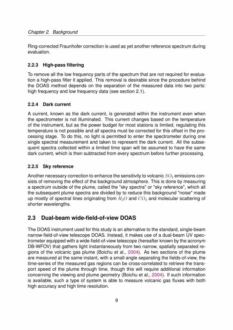
FIGURE 3.4: The final settings used in NovacProgram to evaluate thespectra.

calculating the SO2 fluxes. The final two parameters needed to acquire the flux wasan estimate of the distance to the gas plume and the plume width. The former wasjudged from a map of the area to be about 2000 m, while the latter was calculated bymultiplying the distance to the plume by the field-of-view of the telescope ( 2

15radians).

Only the last 12 days worth of data were considered when calculating the flux val-ues. The reason for this was that the angles the scanner measured at and the scalefactor of the maximum intensity of the measured spectrum were not determined untilthis point. The previous scans, not being optimized to the actual conditions on site,would most likely be difficult to interpret and were therefore excluded from the results.

20

Chapter 4

Results

4.1 Offsets

After calculating the SO2 fluxes using Novac there were a lot of negative values in theresults. Negative values will show up if the "sky reference" spectrum before each setof measurements contain traces of SO2.

On the 23rd of October the instrument was run in "sensitive mode". Figure 4.1shows the measured SO2 emission during the nine hour operating period of the scan-ner. It consists of 34 individual measurements, each containing a clean air sky refer-ence spectrum and 20 individual plume measurement spectra with a duration of 30-45seconds. When evaluating these columns of the plume spectra, each one is dividedby the preceding sky reference to cancel out any background light not relevant to themeasurements. This sky reference should not contain any SO2. However, since thereare negative values for the SO2 emission, the figure below shows this not to be thecase. In each data-set there is a varying degree of offset caused by the sky referencecontaining SO2 traces. These negative numbers can be compensated by including anoffset-level into the flux calculation. This level tells NovacProgram where the "true"zero-level is, and can be calculated automatically or be explicitly specified.

In this case, to compensate for the offsets the plume measurements have beenassumed to be continuous, so that the last measurement of each sequence of mea-surements equals the first measurement of the following sequence. This has beendone in Figure 4.2. This figure shows the calculated SO2 emissions as varying withrespect to the time. Reasons for this variation can be changing degrees of emission,or varying plume speed or plume direction. If a clear sky reference spectrum was notattainable then the figure only shows a relative emission; if a clear sky spectrum wasattainable due to for example a change in wind direction then this value for the skyreference can be used for fixing the offset value. Risking an underestimation of the realemission value, one can assume that if the lowest flux during the day corresponds tolittle or no gas at all, then the span in the emission is an approximation of the actualemission for that day.

21

Chapter 4. Results

FIGURE 4.1: Measurement of the emission from Tavurvur on the 23rd ofOctober done in "sensitive mode".

FIGURE 4.2: The emission measurements from the previous figure aftercorrecting for different offset. The offset correction values are shown in

red.

22

Chapter 4. Results

4.2 SO2 fluxes

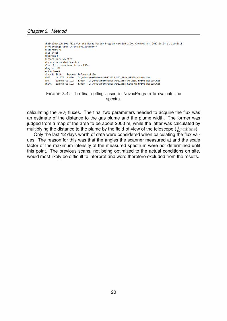
The average SO2 flux during the period 19th to 30th of October 2016 was found to be0.27 kg

s. Two days, the 25th and 26th, were excluded from this period as they were

used to take wind measurements in average flux mode. The variation of the averagesmay be a result of different amount of SO2 in the plume, or because of a change inwind direction or wind speed which would also create an increase or decrease in theSO2 fluxes.

FIGURE 4.3: Each red dot represents the average SO2 flux for that day.The total average over the entire period was found to be 0.27 kg

s .

Wind measurements done in "average flux" mode during the 25th and 26th of Octo-ber. Plume speed used for the SO2 flux calculations was the average of the two days,3.9 ms−1.

23

Chapter 4. Results

FIGURE 4.4: Wind measurement data for the 25th of October, 2016. Theaverage is shown as a red line.

FIGURE 4.5: Wind measurement data from the 26th of October, 2016.The average is shown as a red line.

24

Chapter 5

Discussion

5.1 Wind direction and speed

If the wind direction changes, and instead moves towards or away from the instrument,there will be an increase or decrease in the resulting calculated flux. This is becausethe instruments calculation of the SO2 flux is based on the cross-sections of the plume.If the wind changes and travels towards the instrument then th optical path through theplume, which the instrument integrates along, will be larger then the cross-section andthe resulting flux will be larger as well. If the wind travels away from the instrument, theopposite will instead occur with a resulting flux that is smaller then the actual value.

If there is a significant change in wind speed compared to the values acquiredduring October 25th and October 26th then the SO2 fluxes will be affected since thewind speed is used when calculating the fluxes.

5.2 Recommendation

The plume measurements were done at six degrees above the horizon. Looking atthe clean air sky reference spectra one can see that it was measured at an angle of13 degrees above the horizon. This is only seven degrees different from the plumemeasurements. Given the large wide vertical field of view of the instrument this mostlikely results in the clean air sky reference spectra containing SO2 from the plume. Toavoid this problem the sky reference should be lifted around five to ten degrees in thefuture, to better be able to acquire a dependable sky reference.

25

Chapter 6

Conclusions

The use of a dual-beam wide-field-of-view differential optical absorption spectroscopyinstrument is recommended when measuring low SO2 emissions from Tavurvur vol-cano in Papua New Guinea. This type of instrument at a fixed point close to the pointof emission shows high levels of precision and accuracy and is therefore a viable optionwhen the volcano is degassing at low levels. Due to non-linear effects this wide-field-of-view type of setup is not recommended at high gas emissions but for low activity,as observed in October 2016, this method is applicable at Tavurvur. One must how-ever be careful when obtaining the sky reference spectrum and a recommendation ofincreasing the angle above the horizon that this is measured at by five to ten degreescompared to what was used in this study is proposed. Another consideration to be ob-served is the wind direction: this method will only be useful when the predominant winddirection is perpendicular to the viewing direction of the telescope. This correspondsto a southwestern direction since the instrument is installed at a southeastern location.According to RVO the wind changes during the rainy season and one will then have torethink the location of the instrument site, though these type of measurements mightprove difficult to conduct during this period regardless of wind direction. The DOASinstrument is based on UV detection and relies on sunlight and a clear sky, which is ararity during the rainy season in Papua New Guinea, and the conditions might thereforeprove too difficult for reliable DOAS measurements.

26

Bibliography

Allard, P. et al. (2016). “Prodigious emission rates and magma degassing budget ofmajor, trace and radioactive volatile species from Ambrym basaltic volcano, Van-uatu island Arc”. In: Journal of Volcanology and Geothermal Research 322. Un-derstanding volcanoes in the Vanuatu arc, pp. 119 –143. ISSN: 0377-0273. URL:http://www.sciencedirect.com/science/article/pii/S0377027315003273.

Andres, R.J. and A.D. Kasgnoc (1998). “A time-averaged inventory of subaerial vol-canic sulfur emissions”. In: Journal of Geophysical Research: Atmospheres 103.D19,pp. 25251–25261. ISSN: 2156-2202. DOI: 10.1029/98JD02091. URL: http://dx.doi.org/10.1029/98JD02091.

Arellano, S., B. Galle, and J. Wallius (2017a). “New concept for gas monitoring ofTarvurvur volcano, PNG”. Installation report, unpublished internal document.

— (2017b). “Report on volcanic plume measurements on volcanoes in Papua NewGuinea”. Fieldwork report, unpublished internal document.

Boichu, M. et al. (2004). “High temporal resolution SO2 flux measurements at Erebusvolcano, Antarctica”. In: Journal of Volcanology and Geothermal Research 190,pp. 1455–1470.

Brohede, S. (2002). “Differential Optical Absorption Spectroscopy -How does it workand what can it measure?” In: URL: http://home.elka.pw.edu.pl/~rgraczyk/DOAS.pdf.

Galle, B. et al. (2010). “Network for Observation of Volcanic and Atmospheric Change(NOVAC) - A global network for volcanic gas monitoring: Network layout and instru-ment description”. In: Journal of Geophysical Research 115.

Galle B., et al. (2003). “A miniaturised ultraviolet spectrometer for remote sensing ofSO2 fluxes: a new tool for volcano surveillance”. In: Journal of Volcanology andGeothermal Research 119.1-4, pp. 241–254.

Horton, K.A. et al. (2006). “Real-time measurement of volcanic SO2 emissions: valida-tion of a new UV correlation spectrometer (FLYSPEC)”. In: Bulletin of Volcanology68.4, pp. 323–327. DOI: 10.1007/s00445-005-0014-9. URL: http://dx.doi.org/10.1007/s00445-005-0014-9.

Humaida, H. (2010). “SO2 emission measurement by DOAS (Differential Optical Ab-sorption Spectroscopy) and COSPEC (Correlation Spectroscopy) at Merapi volcano(Indonesia)”. In: Indonesian Journal of Chemistry 8.2. ISSN: 2460-1578. URL: http://pdm-mipa.ugm.ac.id/ojs/index.php/ijc/article/view/358.

Johansson M., et al. (2009). “A miniaturised ultraviolet spectrometer for remote sensingof SO2 fluxes: a new tool for volcano surveillance”. In: Bulletin of Volcanology. DOI:10.1007/s00445-008-0260-8.

27

BIBLIOGRAPHY

Kraus, S. (2006). “DOASIS A Framework Design for DOAS”. PhD thesis. MannheimUniversity.

Lampel, J., U. Friess, and U. Platt (2015). “The impact of vibrational Raman scatter-ing of air on DOAS measurements of atmospheric trace gases”. In: AtmosphericMeasurement Techniques 8.9, pp. 3767–3787. DOI: 10.5194/amt-8-3767-2015.

Mulina, K. (2015). “Monitoring SO2 emissions from Tavurvur volcano, Rabaul, PNG”.NOVAC Project (2017). URL: http://www.novac-project.eu/indexProjectSum.htm.Olmos, R et al. (2007). “Anomalous Emissions of SO2 During the Recent Eruption

of Santa Ana Volcano, El Salvador, Central America”. In: Pure and Applied Geo-physics.

Oppenheimer, C. and JS A. McGonigle (2004). “Exploiting ground-based optical sens-ing technologies for volcanic gas surveillance”. In: Annals of Geophysics 47.4,pp. 1455–1470.

Platt, U. (1994). “Differential optical absorption spectroscopy (DOAS)”. In: Air monitor-ing by spectroscopic techniques, Chem. Anal. Ser. Vol. 127, pp. 27–84.

Platt, U. and D. Perner (1983a). “Measurements of Atmospheric Trace Gases by LongPath Differential UV/Visible Absorption Spectroscopy”. In: Optical and Laser Re-mote Sensing. Ed. by Dennis K. Killinger and Aram Mooradian. Berlin, Heidelberg:Springer Berlin Heidelberg, pp. 97–105. ISBN: 978-3-540-39552-2. DOI: 10.1007/978-3-540-39552-2_13. URL: http://dx.doi.org/10.1007/978-3-540-39552-2_13.

— (1983b). “Measurements of Atmospheric Trace Gases by Long Path DifferentialUV/Visible Absorption Spectroscopy”. In: Optical and Laser Remote Sensing. Ed.by Dennis K. Killinger and Aram Mooradian. Berlin, Heidelberg: Springer Berlin Hei-delberg, pp. 97–105. ISBN: 978-3-540-39552-2. DOI: 10.1007/978-3-540-39552-2_13. URL: http://dx.doi.org/10.1007/978-3-540-39552-2_13.

Sparks, R. S. J. (2003). “Dynamics of magma degassing”. In: Volcanic Degassing.UN World Conference on Disaster Risk and Reduction (2015). URL: http://www.

wcdrr.org/sasakawa/nominees/3907.United States Geological Survey (2015). URL: http://volcanoes.usgs.gov/activity/

methods/gas.php.United States Geological Survey (2016). URL: https://volcanoes.usgs.gov/vhp/

monitoring.html.Volcano Discovery (2017). URL: https : / / www . volcanodiscovery . com / rabaul -

tavurvur.html.Wikipedia (2017). URL: https://en.wikipedia.org/wiki/Rabaul.World Organization of Volcano Observatories (2015). URL: http://www.wovo.org/

0500_0504.html.Wunderman, R. (ed) (1994). “Global Volcanism Program. Report on Rabaul (Papua

New Guinea)”. In: Bulletin of the Global Volcanism Network. Smithsonian Institution.URL: http://dx.doi.org/10.5479/si.GVP.BGVN199408-252140.

28