Embed Size (px)
Citation preview
NEW AUTONOMOUS SENSOR SYSTEM FOR THE CONTINUOUS MONITORING OF THE COMPOSTING PROCES S FROM THE INS IDE
Thesis submitted in partial fulfillment of the requirement for the PhD Degree issued by the Universitat Politècnica de Catalunya, in its Electronic Engineering Program. Francesc Iu Rillo Moral Supervisor: J. Oscar Casas Piedrafita
February 2016

Francesc Iu Rillo Moral: NEW AUTONOMOUS SENSOR SYSTEMFOR THE CONTINUOUS MONITORING OF THE COMPOSTINGPROCESS FROM THE INSIDE, Ph D. Thesis Report, © from Septem-ber 2008 to November 2015

To my grandparents: Ana, Ángeles, Juan and Rafael. In thismoment of maximum maturity they are the link to my chilhood.

Paper stands everything.
— Juan López, engineer
A B S T R A C T
The composting process is Nature’s way of recycling organic wasteswith a good quality organic fertilizer as a result. This process, though,needs of a thoroughly monitoring of temperature and humidityfor a good resulting material. During this Ph.D thesis we devel-oped a wireless temperature and humidity autonomous system thatmonitored from the inside of compost. The fact of measuring andtransmitting from the inside implies the need of a protection forthe circuit and an issue in the measure. Temperature suffers de-lays when measuring from the inside of a protection and, as such,we developed an algorithm, implementable on microcontrollers, tocounteract the effects of first order step responses. Commercial hu-midity sensors need to be in direct contact with the environmentthey are measuring, but that is not possible in compost since theycan get damaged. That is why we designed a humidity sensor basedon coplanar capacitive electrodes that can measure through a protec-tion layer. Compost has never been characterised as a transmissionenvironment, and as such, communications in compost are innova-tive. The heterogeneity of the material and its changes in humidity,temperature and density made the transmission complex. We foundthe proper frequency band to commercially work in compost andthe RF transmission model in compost to estimate attenuation vsdistance.
P U B L I C AT I O N S
As follows the publications resulting from this thesis are listed:
Casas, J. O.; Rillo, F. I. “Method for reducing response time insensor measurement,” Review of Scientific Instruments, 80, 085102
(2009).
v

You have five seconds to enjoy it,and then you remember who you didn’t thank.
— Helen Hunt, actress.
A C K N O W L E D G M E N T S
I would like, first of all, to thank my supervisor, Oscar Casas, for theopportunity, the help, the teachings, the support, the friendship, thescolding and the fun. He is one of the most exceptional persons Ihave ever known and I am proud of being his student.
Next I would like to thank my family for the support. To myparents, Carme and Francesc, for everything I am and will be; to mysister and brother-in-law, Meri and Fer, for their affection; and to mygrandparents, well you know, they are in the dedication.
I would like to thank my very dear friends and colleagues whosupported me with chats, laughs, poker, beers and mojitos. To DaniRodríguez, for he is my best friend; to Davide Vega, who can under-stand my research more than anyone; to Xavier Calvo, one of themost affective persons I have known; Javier López, who perfectlyshares my worries; to Juan López, who is my teacher-colleague-student; to Guillem Enero, beer-poker best guy ever; and to ToniOller, for supporting me when I had no money income at the begin-ning of my PhD. I also want to thank Sara Martínez, for she waspart of my PhD for some time.
I would like to thank the family Aguilera-Esteve for they taught mesomething very valuable: I will be the same person after receivingmy PhD. And yes, my PhD. is about some shit balls that are put intoa fridge with some sensors from the elevators.
I want to thank all the ISI group for their support in my research.Specially to Marcos Quílez, who supervised the communicationsystem for the European Project, to José Polo and to Carles Aliau.Also, thanks to Joan Albesa, the best laboratory mate I had andcould have. Also to Marga López, Oscar Huerta and MontserratSoliva from the Escola Superior d’Agricultura de Barcelona (ESAB).
Moreover, I would like to really thank:Compoball: Novel on-line composting monitoring system. Unió
Europea: FP7-243625-COMPO-BALL. 2010-2013.Composens: Diseño de sistemas de sensores para la vigilancia y
control del proceso de compostaje. DPI2010-14829. Ministerio deciencia e innovación. 2011.
vii

My thesis was developed and funded in the research frameworkof those projects, as well as to the Composting plants from Torrellesand Castelldefels.
Finally I want to thank the Sensors and Instrumentation researchgroup from Graz, that accepted me for three months at their labora-tory. Specially to Hubert Zangl, from whom I learned a lot and toThomas Schlegl, Michael Moser and Thomas Bretterklieber.
I may have forgotten some people to thank, but I normally am avery thankful person so I guess they will not mind, hehe.
viii
C O N T E N T S
1 introduction 1
1.1 State of the art 2
1.2 Objectives 7
2 temperature system 9
2.1 State of the art and proposed solution 9
2.1.1 Proposed solution 10
2.2 Design and Implementation 12
2.3 Sensor conditioning 12
2.3.1 Theoretical models 14
2.3.2 Experimental setup 29
2.3.3 Conclusions 34
2.4 Capsule 35
2.4.1 Material suitability 36
2.4.2 Material influence on the temperature sensor sys-tem 39
2.4.3 Method for reducing response time in sensormeasurement 44
2.5 Conclusions 57
2.6 Experimental tests 58
2.6.1 Lab tests 58
2.6.2 Field tests 62
3 Communication system 67
3.1 State of the art and proposed solution 67
3.1.1 Theoretical model 70
3.2 Compost characterization as a transmission environ-ment 74
3.2.1 Method 74
3.2.2 Experimental setup 74
3.2.3 Results 78
3.3 Experimental tests 81
4 Humidity system 87
4.1 State of the art and proposed solution 87
4.1.1 Proposed solution 89
4.2 Compost relative permittivity 91
4.2.1 Parallel plate capacitor 91
4.2.2 concentric cylinder capacitor 98
4.3 Coplanar electrode study and design 104
4.4 Single-layer coplanar capacitive electrodes 104
4.4.1 General problem description 105
ix
x Contents
4.4.2 Theoretical models 106
4.4.3 Simulation 108
4.4.4 Experimental results 120
4.4.5 Conclusions 125
4.5 Multilayer coplanar capacitive electrodes 126
4.5.1 Theoretical models 127
4.5.2 Simulation 129
4.5.3 Experimental results 141
4.5.4 Conclusions 144
4.6 Final electrode calibration 145
4.7 Electrode design conclusion 146
5 conclusions 148
Appendix 151
a temperature system component selection 152
a.1 Microcontroller 152
a.2 Sensor 154
a.3 Real-time-clock (RTC) 154
a.4 Electrically Erasable Programmable Read-Only Mem-ory (EEPROM) 156
a.5 Voltage regulator 157
a.6 Batteries 158
b need of protection 160
b.1 Physical protection 160
b.2 Chemical protection 161
b.3 Thermal and humidity protection 161
c thermal conductivity 164
bibliography 167
L I S T O F F I G U R E S
Figure 1 Composting process (Source: Composting man-ual. Alberta government. Canada) 2
Figure 2 Composting process temperature evolution (ex-tracted from [2]) 3
Figure 3 Composting process humidity evolution (extractedfrom [3]) 3
Figure 4 (a) Classic conditioning. (b) Classic condition-ing without dynamic range adjustment. (c) directsensor-to-microcontroller interface. 13
Figure 5 Sensor stage option (a) current flow 16
Figure 6 Sensor stage option (b) current flow 16
Figure 7 Direct sensor-to-microcontroller interface (threesignal method) 22
Figure 8 Energy consumption vs effective number of bits(α = 0.1). Points of each series are, from left toright, 20, 17.6, . . . , 0.538, 0.473 Hz. For a 16 bitADC. 26
Figure 9 Energy consumption vs effective number of bits(k1 = 0.1185). Points of each series are, from leftto right, 20, 17.6, . . . , 0.538, 0.473 Hz. For a 16 bitADC. 26
Figure 10 Energy consumption vs effective number of bits(α = 0.1). f = 20 Hz 27
Figure 11 Energy consumption vs effective number of bits(k1 = 0.1185). f=20 Hz. 27
Figure 12 Energy consumption vs effective number of bits(α = 0.1). f = 0,145 Hz. Using 24 bit ADC. 28
Figure 13 Energy consumption vs effective number of bits(k1 = 0.1185). f=0.145 Hz. Using 24 bit ADC. 28
Figure 14 Voltage in function of time for the case of alphaequal to 0.0720 32
Figure 15 Voltage histogram for the case of alpha equal to0.0720 32
Figure 16 Calibration of R measured 33
Figure 17 FCH climatic chamber used in our tests 36
Figure 18 Capsules after the test in an urban composter 37
Figure 19 (a) Capsules before the test. (b) Capsules afterthe test (only the ones recovered). 38
xi
xii List of Figures
Figure 20 Samples taken on a first order system (Vo <
Vf) 46
Figure 21 Resulting equations 47
Figure 22 Uncertainty of Equation (7) for dy1/Vf = dy2/Vf =
dy3/Vf = [0.001, 0.01] in function of ∆t 47
Figure 23 Error of the calculation depending on when thelast sample (time measured tm) was taken, usingthe different equations (8-bit systems) 49
Figure 24 Error of the calculation depending on when thelast sample (time measured tm) was taken, usingthe different equations (10-bit systems) 50
Figure 25 Error of the different equations applied to thecharge acquired with the oscilloscope 53
Figure 26 Error of the different equations applied to thedischarge acquired with the oscilloscope 53
Figure 27 Error of the different equations applied to thecharge acquired with the DAQ 54
Figure 28 Error of the different equations applied to thedischarge acquired with the DAQ 54
Figure 29 Circuit inserted into the High Bouncing balls 59
Figure 30 Measure inside the capsule of the answer to atemperature step. 60
Figure 31 Measure inside the capsule (1 sample per mea-sure) 60
Figure 32 Uncertainty of applying the method to the exper-imental data 61
Figure 33 Pot measures distribution 61
Figure 34 Results of measuring inside ground 62
Figure 35 Pile in maturing stage 62
Figure 36 Result of the second test inside the compost pile 63
Figure 37 Composter 64
Figure 38 Test inside the composter 64
Figure 39 Our sensor with four probes attached to its sur-face with a 90 ° 65
Figure 40 Test inside pile for two months 66
Figure 41 Theoretical transmission through compost 67
Figure 42 Humidity evolution (extracted from [3]) 68
Figure 43 Density evolution (extracted from Table 3.2 from[75]) 68
Figure 44 Qualitative evolution of humidity and densityduring the composting process 69
Figure 45 Characterization method 74
List of Figures xiii
Figure 46 Experimental setup. (left) Signal generator andgain amplifier. (right) Spectrum analyzer. 75
Figure 47 Power propagation model 75
Figure 48 Gain characterization 76
Figure 49 Dipole antenna factor characterization 77
Figure 50 Dipole antenna factor repeatability 77
Figure 51 Air-compost comparison 78
Figure 52 Air-soil comparison 79
Figure 53 Signal and noise repeatability. (a) Air. (b) Com-post. 80
Figure 54 Antenna inside ball before closing 81
Figure 55 Antenna factor characterization 82
Figure 56 Theoretical and experimental transmission model.(a) Air. (b) Compost. 83
Figure 57 Compost theoretical transmission model for 1/d3
attenuation 84
Figure 58 Distance attenuation coefficient uncertainty 85
Figure 59 Coplanar capacitive electrode 90
Figure 60 Experimental setup 92
Figure 61 Electric equivalent model of the parallel plateswith air 93
Figure 62 Electric equivalent model of the parallel plateswith compost 94
Figure 63 T electric model of the parallel plates with com-post 94
Figure 64 T with serial resistance equivalent model of theparallel plates with compost 95
Figure 65 Impedance temperature and frequency behav-ior 96
Figure 66 Error temperature and frequency behavior 96
Figure 67 Impedance humidity and frequency behavior 97
Figure 68 Impedance density and frequency behavior 98
Figure 69 Cylinder dimensions 99
Figure 70 Compost dielectric characterization method 100
Figure 71 Experimental setup 101
Figure 72 Experimental setup equivalent electric model 101
Figure 73 Theoretical model applied to experimental test 101
Figure 74 Relative permittivity of compost in function ofthe relative humidity 102
Figure 75 3D Interdigital electrodes 107
Figure 76 3D Concentric electrodes 110
Figure 77 Nominal Capacitance change in function of lsep 110
Figure 78 Capacitance change in function of lsep 111
xiv List of Figures
Figure 79 Capacitance change over Nominal Capacitancein function of lsep 111
Figure 80 Nominal Capacitance in function of ra 112
Figure 81 Capacitance change in function of ra 112
Figure 82 Capacitance change over Nominal Capacitancein function of ra 113
Figure 83 Difference between the concentric simulation andthe theoretical model capacitance 114
Figure 84 Nominal Capacitance in function of lsep 115
Figure 85 Capacitance change in function of lsep 115
Figure 86 Capacitance change over Nominal Capacitancein function of lsep 116
Figure 87 Nominal Capacitance in function of lteeth 116
Figure 88 Capacitance change in function of lteeth 117
Figure 89 Capacitance change over Nominal Capacitancein function of lteeth 117
Figure 90 Nominal Capacitance in function of N 118
Figure 91 Capacitance change in function of N 118
Figure 92 Capacitance change over Nominal Capacitancein function of N 119
Figure 93 Difference between the interdigital simulationand the theoretical model capacitance 120
Figure 94 Experimental concentric electrodes 121
Figure 95 Experimental interdigital electrodes 123
Figure 96 Histogram of the ε1/ε2 relation of the theoreticalmodel applied to all the experimental cases 125
Figure 97 3D Concentric electrodes inside ball 129
Figure 98 Nominal Capacitance change in function of lsep 130
Figure 99 Capacitance change in function of lsep 131
Figure 100 Capacitance change over Nominal Capacitancein function of lsep 131
Figure 101 Nominal Capacitance in function of ra 132
Figure 102 Capacitance change in function of ra 132
Figure 103 Capacitance change over Nominal Capacitancein function of ra 133
Figure 104 3D Interdigital electrodes inside ball 134
Figure 105 Nominal Capacitance in function of lsep 134
Figure 106 Capacitance change in function of lsep 135
Figure 107 Capacitance change over Nominal Capacitancein function of lsep 135
Figure 108 Nominal Capacitance in function of lteeth 136
Figure 109 Capacitance change in function of lteeth 136
Figure 110 Capacitance change over Nominal Capacitancein function of lteeth 137
Figure 111 Nominal Capacitance in function of N 138
Figure 112 Capacitance change in function of N 138
Figure 113 Capacitance change over Nominal Capacitancein function of N 139
Figure 114 Nominal Capacitance in function of lsep 139
Figure 115 Capacitance change in function of lsep 140
Figure 116 Capacitance change over Nominal Capacitancein function of lsep 140
Figure 117 Experimental setup 141
Figure 118 Experimental concentric electrodes 142
Figure 119 Experimental interdigital electrodes 143
Figure 120 Voltage regulator circuit provided by the man-ufacturer (Taken from 5V/3.3V or Adjustable,Low-Dropout Low Iq, 200mA Linear RegulatorsDatasheet) 158
Figure 121 Compost turner [130] 160
Figure 122 Composting temperature evolution [132] 162
Figure 123 Composting humidity evolution 163
Figure 124 (left) Circuit acquiring the temperature of the fo-cus around it. (right) circuit playing as a thermalconductor between focus. 164
L I S T O F TA B L E S
Table 1 ENOB and energy of using the direct sensor-to-microcontroller interface 28
Table 2 Consumption experimental vs theoretical results(α constant) 30
Table 3 Consumption experimental vs theoretical results(k1 constant) 30
Table 4 Experimental and theoretical ENOB in functionof k1 31
Table 5 Experimental and theoretical ENOB in functionof α 31
Table 6 Experimental measure of the ENOB 34
Table 7 Changes in the weight after the composting pro-cess in the composter 37
xv
xvi List of Tables
Table 8 Changes in the weight after the composting pro-cess in the pile 38
Table 9 0.6 cm measured magnitudes [63] 40
Table 10 1.2 cm measured magnitudes [63] 41
Table 11 0.8 cm measured magnitudes [63] 42
Table 12 1.8 cm measured magnitudes [63] 42
Table 13 0.4 cm measured magnitudes [63] 43
Table 14 Relation between tm and τ for 8-bit systems 50
Table 15 Relation between tm and τ for 10-bit systems 51
Table 16 Maximal error of the experimental and theoreti-cal results from 2.5·τ (8-bit) and 4.0·τ (10-bit) to10·τ (numbers between brackets in the table cor-respond to the application of the equations withtheoretically generated data) 55
Table 17 Mean and standard deviation of the error of theexperimental and theoretical results in tm =2.5·τ(8-bit) and 4.0·τ (10-bit) and its 4 consecutivepoints (numbers between brackets in the tablecorrespond to the application of the equationswith theoretically generated data) 56
Table 18 Continuous measure test results 59
Table 19 Experimental measures with our sensor and fourprobes attached to its surface 65
Table 20 Humidity measure method comparative 88
Table 21 Theoretical relative permittivity in function ofthe composting process ranges of humidity anddensity 103
Table 22 Coeficient result 113
Table 23 Coeficient result 119
Table 24 Concentric electrodes experimental performancein function of lsep 122
Table 25 Theoretical model applied to the experimentalperformance in function of lsep 122
Table 26 Concentric electrodes experimental performancein function of ra 122
Table 27 Theoretical model applied to the experimentalperformance in function of ra 122
Table 28 Interdigital electrodes experimental performancein function of ls 124
Table 29 Theoretical model applied to the experimentalperformance in function of ls 124
Table 30 Interdigital electrodes experimental performancein function of lteeth 124
Table 31 Theoretical model applied to the experimentalperformance in function of lteeth 124
Table 32 Interdigital electrodes experimental performancein function of #teeth 125
Table 33 Theoretical model applied to the experimentalperformance in function of #teeth 125
Table 34 Interdigital vs Concentric electrode performance 138
Table 35 Concentric electrodes experimental performancein function of lsep 142
Table 36 Concentric electrodes experimental performancein function of ra 142
Table 37 Interdigital electrodes experimental performancein function of ls 143
Table 38 Interdigital electrodes experimental performancein function of lteeth 144
Table 39 Interdigital electrodes experimental performancein function of #teeth 144
Table 40 Parallel electrodes experimental performance infunction of ls 144
Table 41 Texas Instruments MCUs comparative 153
Table 42 Commercial Temperature sensors 155
Table 43 Minimal prize within the RTC fulfilling the speci-fied requirements (data according to Farnell) 155
Table 44 Comparative of the different manufacturer RTCdevices 156
Table 45 Comparative of the different manufacturer EEP-ROM devices 157
Table 46 Temperature system consumption 159
xvii
xviii acronyms
Table 47 Heat generation of different molecules [132] 162
L I S T O F A L G O R I T H M S
A C R O N Y M S
ACK Acknowledgement
CEPT European Conference of Postal and TelecommunicationsAdministrations
CPU Control Processing Unit
DAQ Data Acquisition
EC European Community
EEPROM Electrically Erasable Programmable Read Only Memory
ERC European Radiocommunications Committee
EU European Union
FSS Frequency Selective Surface
I2C Inter-Integrated Circuit
IC Integrated Circuit
ISM Industrial, Scientific and Medical
IP Ingress Protection
MCU MicroController Unit
PET Polyethylene Terephthalate
PMR Personal Mobile Radio
PP PolyPropylene
acronyms xix
PS PolyStyrene
PU Polyurethane
PVC PolyVinyl Chloride
RAM Random Access Memory
RC Resistance-Capacitance
RH Relative Humidity
RS232 Recommended Standard 232
RTD Resistance Temperature Detector
RF RadioFrequency
RFID RadioFrequency IDentification
SNR Signal-to-Noise-Ratio
SoC State of Charge
SoH State of Health
UART Universal Asynchronous Receiver Transmitter

Sigmund Freud was a novelist with a scientific background.He just didn’t know he was a novelist.All those damn psychiatrists after him,
they didn’t know he was a novelist either.
— John Irving, novelist
1I N T R O D U C T I O N
Composting is Nature’s way of recycling and represents a sustain-able solution for the treatment of organic waste, whatever its origin.It is a natural biological process, carried out under controlled aerobicconditions, whereby various microorganisms, including bacteria andfungi, break down organic matter into an organic fertilizer. Sinceapproximately 45 % to 55 % of the waste stream is organic matter,composting can play a significant role in diverting waste from land-fills thereby conserving landfill space and reducing the productionof leachates and methane gas.
The composting process requires of a good previous planing butalso of a right monitoring of the control parameters. Being an aerobic,bio-oxidative and thermophile process the main parameters thatpermit interpreting what is happening are the temperature and thewater evolution. If the initial mix is adequate and it has a correcthumidity and oxygen concentration values, the composting materialheats up as a result of the degradation activity of the microorganismsworking in. As a thermophile process it is mandatory to maintain aminimal temperature, in order to clean the material, and it is alsomandatory to maintain the temperature level not too high since itcan end up affecting the decomposing microorganisms. Also, wateris essential to sustain microorganisms, although if too much theydie. Therefore, controlling temperature and humidity through timeis a key factor to obtain good results.
Currently there is a lack of thoroughness in the composting processmonitoring. This work aims to develop new proposals in the measureof temperature and humidity in compost, allowing optimizing theinstrumentation and communication in terms of power consumption,cost and size. With field tests realized at the composting plant wewill develop some guidelines and proper procedures to optimize thecomposting process, in order to increase the quality of the resultingproduct.
1
2 introduction
1.1 state of the art
Composting plants are the locations where urban organic wastes arebrought, in order to enter into the composting process to produceorganic fertilizers.
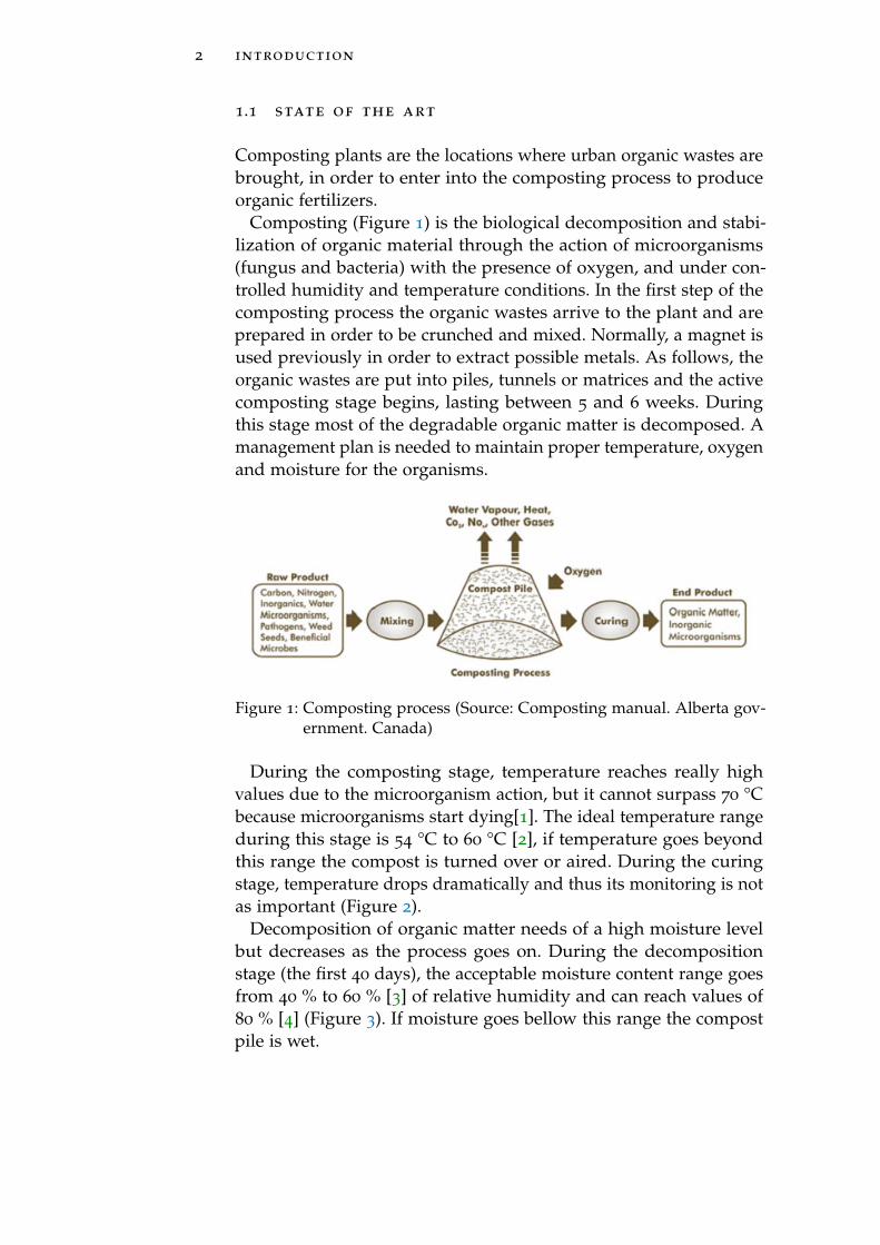
Composting (Figure 1) is the biological decomposition and stabi-lization of organic material through the action of microorganisms(fungus and bacteria) with the presence of oxygen, and under con-trolled humidity and temperature conditions. In the first step of thecomposting process the organic wastes arrive to the plant and areprepared in order to be crunched and mixed. Normally, a magnet isused previously in order to extract possible metals. As follows, theorganic wastes are put into piles, tunnels or matrices and the activecomposting stage begins, lasting between 5 and 6 weeks. Duringthis stage most of the degradable organic matter is decomposed. Amanagement plan is needed to maintain proper temperature, oxygenand moisture for the organisms.
Figure 1: Composting process (Source: Composting manual. Alberta gov-ernment. Canada)
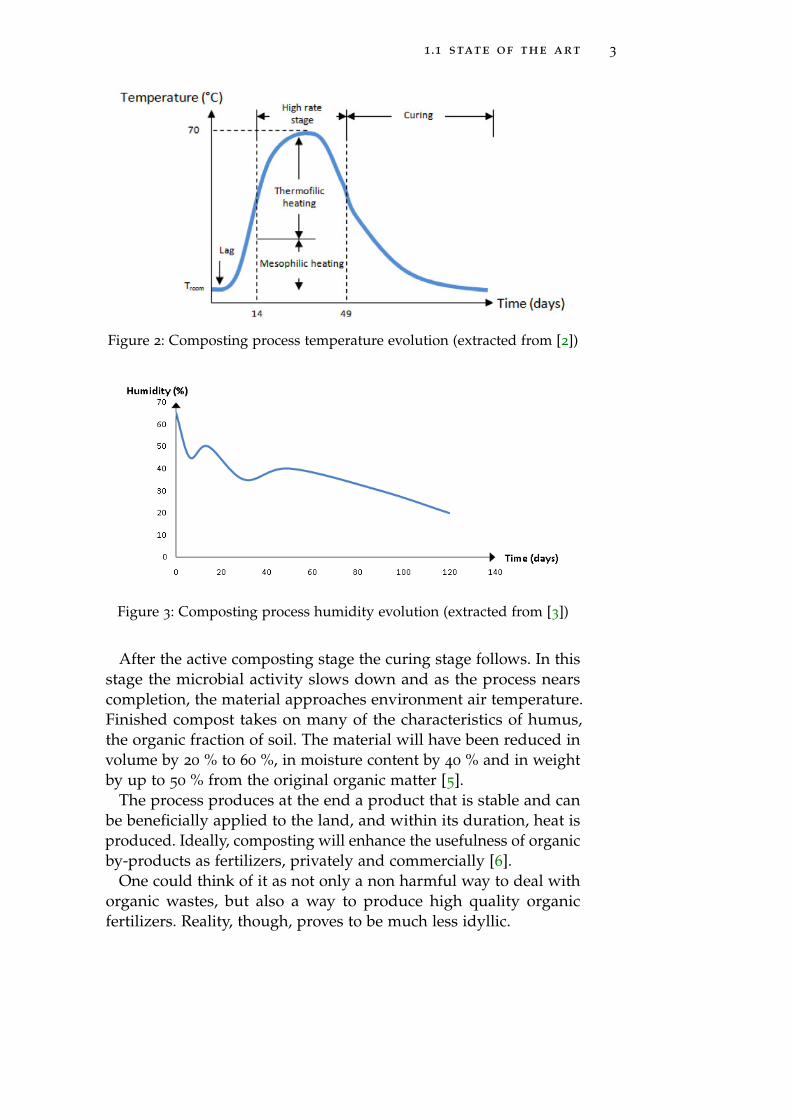
During the composting stage, temperature reaches really highvalues due to the microorganism action, but it cannot surpass 70 °Cbecause microorganisms start dying[1]. The ideal temperature rangeduring this stage is 54 °C to 60 °C [2], if temperature goes beyondthis range the compost is turned over or aired. During the curingstage, temperature drops dramatically and thus its monitoring is notas important (Figure 2).
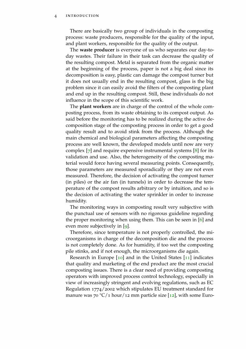
Decomposition of organic matter needs of a high moisture levelbut decreases as the process goes on. During the decompositionstage (the first 40 days), the acceptable moisture content range goesfrom 40 % to 60 % [3] of relative humidity and can reach values of80 % [4] (Figure 3). If moisture goes bellow this range the compostpile is wet.
1.1 state of the art 3
Figure 2: Composting process temperature evolution (extracted from [2])
Figure 3: Composting process humidity evolution (extracted from [3])
After the active composting stage the curing stage follows. In thisstage the microbial activity slows down and as the process nearscompletion, the material approaches environment air temperature.Finished compost takes on many of the characteristics of humus,the organic fraction of soil. The material will have been reduced involume by 20 % to 60 %, in moisture content by 40 % and in weightby up to 50 % from the original organic matter [5].
The process produces at the end a product that is stable and canbe beneficially applied to the land, and within its duration, heat isproduced. Ideally, composting will enhance the usefulness of organicby-products as fertilizers, privately and commercially [6].
One could think of it as not only a non harmful way to deal withorganic wastes, but also a way to produce high quality organicfertilizers. Reality, though, proves to be much less idyllic.
4 introduction
There are basically two group of individuals in the compostingprocess: waste producers, responsible for the quality of the input,and plant workers, responsible for the quality of the output.
The waste producer is everyone of us who separates our day-to-day wastes. Their failure in their task can decrease the quality ofthe resulting compost. Metal is separated from the organic matterat the beginning of the process, paper is not a big deal since itsdecomposition is easy, plastic can damage the compost turner butit does not usually end in the resulting compost, glass is the bigproblem since it can easily avoid the filters of the composting plantand end up in the resulting compost. Still, these individuals do notinfluence in the scope of this scientific work.
The plant workers are in charge of the control of the whole com-posting process, from its waste obtaining to its compost output. Assaid before the monitoring has to be realized during the active de-composition stage of the composting process in order to get a goodquality result and to avoid stink from the process. Although themain chemical and biological parameters affecting the compostingprocess are well known, the developed models until now are verycomplex [7] and require expensive instrumental systems [8] for itsvalidation and use. Also, the heterogeneity of the composting ma-terial would force having several measuring points. Consequently,those parameters are measured sporadically or they are not evenmeasured. Therefore, the decision of activating the compost turner(in piles) or the air fan (in tunnels) in order to decrease the tem-perature of the compost results arbitrary or by intuition, and so isthe decision of activating the water sprinkler in order to increasehumidity.
The monitoring ways in composting result very subjective withthe punctual use of sensors with no rigorous guideline regardingthe proper monitoring when using them. This can be seen in [6] andeven more subjectively in [9].
Therefore, since temperature is not properly controlled, the mi-croorganisms in charge of the decomposition die and the processis not completely done. As for humidity, if too wet the compostingpile stinks, and if not enough, the microorganisms die again.
Research in Europe [10] and in the United States [11] indicatesthat quality and marketing of the end product are the most crucialcomposting issues. There is a clear need of providing compostingoperators with improved process control technology, especially inview of increasingly stringent and evolving regulations, such as ECRegulation 1774/2002 which stipulates EU treatment standard formanure was 70 °C/1 hour/12 mm particle size [12], with some Euro-
1.1 state of the art 5
pean countries imposing this only for products intended to be tradedinternationally. EC Regulation 208/2006 allows for the approval ofalternative composting and bio gas standards for the treatment ofanimal by-products, whereby rather than setting out the processrequirements (time/temperature/particle size) for treatment of rawmaterial it permits the operator specifying their own treatmentparameters, provided that the operator can demonstrate throughmicrobiological testing of the finished product that the system hasproduced sufficient pathogen reduction (and of course providedthe system still complies with all other aspects of 1774/2002). Suchregulations, along with market demands for high quality, stable andsafe composting are clear drivers for bridging the current gaps incompost monitoring and control technology.
Each country in the world has its own regulations to measurethe quality of the resulting compost [13]. Still, the procedure issimilar, the only change resides on the level of particles. A sample ofcompost is taken, isolating it in order to avoid contamination, andbrought into a laboratory [14]. Once there, the levels of heavy metalsand pathogens are measured and compared to the acceptable levelsto decide whether it has a good quality or not.
This work will guide a research effort in the development of anon-line wireless system that will be effective for the measurement ofboth temperature and humidity at various points in the compostingmaterial.
Since compost is a heterogeneous material higher temperatureswill be produced in punctual focus inside the composting material.Furthermore, current probes can be affected by external conditions.Thus, measures have to be realized from the inside. However, anenclosure for the circuit is needed to isolate the system from haz-ardous substances and from humidity. This enclosure will have tostand blows due to the action of the compost turner. For furtherinformation regarding the need of protection refer to Appendix B.
The fundamental material used for industrial and electrical isola-tion is the family of polymers [15]. But in front of high temperatureswe have to discard Polyvinyl chloride (PVC) because it melts attemperatures of 80 °C [16] (and it becomes deformed earlier) andthe blows of the compost turner makes Polyethylene terephthalate(PET) to be also discarded since its hardness is so great [17] that itcan jam the shovels of the compost turner. Polystyrene (PS) is alsodiscarded due to its low impact strength [18] along with Polypropy-lene (PP) [19]. Polyurethane (PU) on another hand has a high impactstrength and high melting point (107 °C) [20], but it provides ther-mal isolation which will increase the transference of temperature
6 introduction
(which we have already considered when talking of temperature).Silicone has similar properties to PU but it has a great heat transfer-ence, which would make it ideal if it were not for its opposition tomicrobiological growth [21].
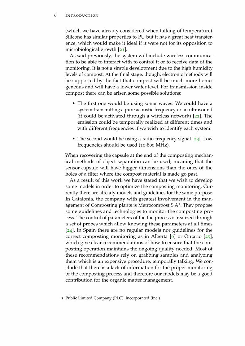
As said previously, the system will include wireless communica-tion to be able to interact with to control it or to receive data of themonitoring. It is not a simple development due to the high humiditylevels of compost. At the final stage, though, electronic methods willbe supported by the fact that compost will be much more homo-geneous and will have a lower water level. For transmission insidecompost there can be arisen some possible solutions:
• The first one would be using sonar waves. We could have asystem transmitting a pure acoustic frequency or an ultrasound(it could be activated through a wireless network) [22]. Theemission could be temporally realized at different times andwith different frequencies if we wish to identify each system.
• The second would be using a radio-frequency signal [23]. Lowfrequencies should be used (10-800 MHz).
When recovering the capsule at the end of the composting mechan-ical methods of object separation can be used, meaning that thesensor-capsule will have bigger dimensions than the ones of theholes of a filter where the compost material is made go past.
As a result of this work we have stated that we wish to developsome models in order to optimize the composting monitoring. Cur-rently there are already models and guidelines for the same purpose.In Catalonia, the company with greatest involvement in the man-agement of Composting plants is Metrocompost S.A1. They proposesome guidelines and technologies to monitor the composting pro-cess. The control of parameters of the the process is realized througha set of probes which allow knowing these parameters at all times[24]. In Spain there are no regular models nor guidelines for thecorrect composting monitoring as in Alberta [6] or Ontario [25],which give clear recommendations of how to ensure that the com-posting operation maintains the ongoing quality needed. Most ofthese recommendations rely on grabbing samples and analyzingthem which is an expensive procedure, temporally talking. We con-clude that there is a lack of information for the proper monitoringof the composting process and therefore our models may be a goodcontribution for the organic matter management.
1 Public Limited Company (PLC). Incorporated (Inc.)
1.2 objectives 7
1.2 objectives
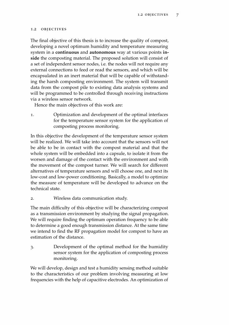
The final objective of this thesis is to increase the quality of compost,developing a novel optimum humidity and temperature measuringsystem in a continuous and autonomous way at various points in-side the composting material. The proposed solution will consist ofa set of independent sensor nodes, i.e. the nodes will not require anyexternal connections to feed or read the sensors, and which will beencapsulated in an inert material that will be capable of withstand-ing the harsh composting environment. The system will transmitdata from the compost pile to existing data analysis systems andwill be programmed to be controlled through receiving instructionsvia a wireless sensor network.
Hence the main objectives of this work are:
1. Optimization and development of the optimal interfacesfor the temperature sensor system for the application ofcomposting process monitoring.
In this objective the development of the temperature sensor systemwill be realized. We will take into account that the sensors will notbe able to be in contact with the compost material and that thewhole system will be embedded into a capsule, to isolate it from theworsen and damage of the contact with the environment and withthe movement of the compost turner. We will search for differentalternatives of temperature sensors and will choose one, and next itslow-cost and low-power conditioning. Basically, a model to optimizethe measure of temperature will be developed to advance on thetechnical state.
2. Wireless data communication study.
The main difficulty of this objective will be characterizing compostas a transmission environment by studying the signal propagation.We will require finding the optimum operation frequency to be ableto determine a good enough transmission distance. At the same timewe intend to find the RF propagation model for compost to have anestimation of the distance.
3. Development of the optimal method for the humiditysensor system for the application of composting processmonitoring.
We will develop, design and test a humidity sensing method suitableto the characteristics of our problem involving measuring at lowfrequencies with the help of capacitive electrodes. An optimization of

8 introduction
the design of the measuring electrodes will be realized to maximizethe sensitvity of the sensor. We will not focus on the electronicsinvolved into the sensor system but on the physics, since that doesnot involve any improvement in the current state of the art.
Everything popular is wrong.
— Oscar Wilde, dramatist
2T E M P E R AT U R E S Y S T E M
2.1 state of the art and proposed solution
As stated in the Objectives, in this chapter and the following oneswe will develop a temperature system for the autonomous measureof compost from the inside with a protection. To do so, we first needto know what the current solutions are and identify the problemsagainst the improvements we can offer.
We have seen, that for temperature monitoring in compostingthe most extended use is the insertion of probes [26, 27]. Thereare many manufacturers involved in their distribution, some ofthem innovating with probes that are left put and communicatevia wireless with a transceiver [28]. The idea of wireless sensors issupported and evolved to wireless sensor networks as in the patent[29] and in the products of [30]. The problem of this kind of productis that it results expensive and it has to be removed in order to turnover the compost material. This last problem is really old and eventhe possibility of inserting sensors in the turner shovels was arisenin some patents [31], but that is nonsense since the compost turneris activated only when the measured temperature is above somelimited temperature levels.
A part from the probe insertion, there are really few solutions forthe control of temperature; the following one refers to its monitoringon tunnels where no turning is realized and where the answer infront of a too high temperature is the action of a fan [32]. This cannotbe extrapolated to other enclosures rather than tunnels. Therefore, asstated before, a good solution would be a sensor system measuringfrom the inside and protected enough to stand the blows of thecompost turner (with an elastic protective enclosure) and to protectit from humidity (hence a minimum IP 67 grade is needed). Theproblem of a sensor inside a capsule is the delay due to the thermalcapacitance that implies. In order to know what the temperatureoutside the capsule is we can use a method to estimate what thetransient of the temperature sensor tends to [33].
9
10 temperature system
On the other hand, to have a proper monitoring of the compostingprocess a continuous measurement is needed. The time intervalbetween samples has to be adaptable because temperature changesduring the active decomposition stage are dependent of the locationand the processing time. Temperature changes very slowly duringthe whole composting process and its values may vary half a degreeper hour, and so a measuring rate of at least 30 min is more thanenough for the monitoring of temperature.
If the system has to be measuring from the inside during the wholecomposting process autonomously, we will need to minimize thesystem consumption as much as possible. The basics for this will bebased on a low-consumption microcontroller, one that allows exactlycontrolling which part of the microcontroller is active at each time,incredibly optimizing the overall consumption [34]. As said before,temperature changes in compost are really slow, this permits usingthe method to estimate the tendency of a first order transient [33],with which we will save taking at least 40 % of the samples of atransient.
We wish to elaborate a scalable product; meaning one able tobe used in all kind of composting enclosures, therefore its prizehas to be the minimum possible. To minimize its prize we coulddecrease the number of components; like using a conditioning of adirect sensor to microcontroller interface [35] or other conditioningtechniques like Dynamic Power Management [36]. The compostingprocess lasts around 2 months and as such, the batteries should beable to stand at least this time supplying the system.
2.1.1 Proposed solution
Our system is wished to be adaptable basically to different compost-ing enclosures, like tunnels and piles, and to the different environ-ments of geographical zones all over the world. Also it would beinteresting to be able to use this same system on other processesrather than in composting enclosures, as for example in silos. Themain and only critical changing factor of this adaptability is thetime that the process lasts. With the development of a programminginterface, the final user would be able to define the time of eachstage of the process for the sensor system to act consequently.
As said in Chapter 1 the maximum temperature during the com-posting process is of 70 °C, therefore we will look for an electronicsystem able to work at this temperature or even until 80 °C just tohave some margin. An accuracy of 0.3 °C and a precision of 0.1 °Cis required by definition from the European project Compoball in

2.1 state of the art and proposed solution 11
which this thesis have been developed, which agrees to the standardregulations of the European Union in the measure of temperature incompost.
Therefore, in this part of the Thesis we will develop a Temperaturesystem that works autonomously inside compost protected by anelastic enclosure (IP67 to be able to protect both from water andchemical attacks) and supplied by some batteries, during around 2
months (which is the time a whole composting process lasts). Thesystem will measure with an adaptable rate of at least 30 minutesand will keep the measures, with the time in which they were taken,in order to be able to see the evolution afterward.
12 temperature system
2.2 design and implementation
The design and implementation of the Temperature system willfocus on the conditioning of the sensor and everything related tothe measure of temperature which will be what will determine theconsumption of the system in front of the quality in the measure.
On the other hand, our system has to be embedded into a capsuleas said in chapter 2, therefore in order to fit our circuit inside acapsule we have to consider minimizing its size and the size of all itscomponents. Moreover, we find that the duration of the batteries hasto last the whole composting process, and thus the components musthave the minimal consumption. Besides, the composting processcan reach values of temperature up to 70
C, and so the operatingtemperature of our devices has to be over this value. Furthermore,we have specified that we wish to produce a scalable final product;therefore the total prize has to be the lowest.
In Appendix A the selection and justification of all the devicesin the architecture can be found. As follows we will explain theinnovative parts which are the sensor conditioning and the protectivecapsule.
2.3 sensor conditioning
Our sensor conditioning has to be applied to detect the changes ofthe resisting sensor with the highest resolution-consumption rate.There are many solutions to reduce consumption and to improve theresolution, we will find a balanced one for our system. As followsthe different alternatives in the bibliography are described.
Typically, to reduce analog and digital consumption a DynamicPower Management (DPM) is commonly used (wake-up methods[37]),consisting on a sensor system remaining in different sleep timeseffectively reducing the consumption as long as the sleep time ismuch bigger than the active stage time. Another method commonlylinked to the DPM is the Dynamic Voltage Scaling (DVS) for digitalconsumption reduction. While DPM reduces the overall consump-tion using low power modes, it is possible to have an additionalenergy saving if in the active stages the parts of the microcontrollernot used are switched off. A part from the previous alternatives,the bibliography offers other less common solutions for digital con-sumption reduction, as including optimal synchronization of thecommunications[38] or optimizing pre-processing operations[39].Another extended solution is the reduction of the clock in the mi-
2.3 sensor conditioning 13
crocontroller to reduc consumption (e.g use 32 kHz instead of 8
MHz).A part from DPM, a very extended solution to reduce the number
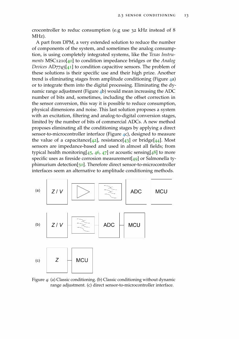
of components of the system, and sometimes the analog consump-tion, is using completely integrated systems, like the Texas Instru-ments MSC1210[40] to condition impedance bridges or the AnalogDevices AD7745[41] to condition capacitive sensors. The problem ofthese solutions is their specific use and their high prize. Anothertrend is eliminating stages from amplitude conditioning (Figure 4a)or to integrate them into the digital processing. Eliminating the dy-namic range adjustment (Figure 4b) would mean increasing the ADCnumber of bits and, sometimes, including the offset correction inthe sensor conversion, this way it is possible to reduce consumption,physical dimensions and noise. This last solution proposes a systemwith an excitation, filtering and analog-to-digital conversion stages,limited by the number of bits of commercial ADCs. A new methodproposes eliminating all the conditioning stages by applying a directsensor-to-microcontroller interface (Figure 4c), designed to measurethe value of a capacitance[42], resistance[43] or bridge[44]. Mostsensors are impedance-based and used in almost all fields; fromtypical health monitoring[45, 46, 47] or acoustic sensing[48] to morespecific uses as fireside corrosion measurement[49] or Salmonella ty-phimurium detection[50]. Therefore direct sensor-to-microcontrollerinterfaces seem an alternative to amplitude conditioning methods.
Figure 4: (a) Classic conditioning. (b) Classic conditioning without dynamicrange adjustment. (c) direct sensor-to-microcontroller interface.
14 temperature system
Hitherto, no systematic study has been realized to compare theconsumption and effective resolution trade-off of the different con-ditioning alternatives, to see how the design is affected. Thus, ourobjective is comparing the performance of amplitude conditioningmethods with direct sensor-to-microcontroller interfaces, by study-ing the consumption vs the effective resolution of each system. Thisway we would find out which is the most efficient sensor condition-ing technique for our system.
2.3.1 Theoretical models
The alternatives for classic amplitude conditioning systems anddirect sensor-to-microcontroller interfaces are explained in the fol-lowing subsections. In classic conditioning systems, reactive sensorsneed of an AC excitation voltage or current, that implies additionallyusing a demodulator in front of the DC excitation needed on resis-tive sensors. For direct sensor-to-microcontroller interfaces the useof a resistive or a capacitive sensor does not matter and thus, if theconsumption and noise were to be reduced using a resistive sensor(which we have not proven yet), in the case of using a capacitivesensor would be even better since the demodulator is not necessary.
Hence, the use of a resistive sensor as the input will serve also asa reference for the use of capacitive sensors.
Amplitude conditioning
Amplitude signal conditioning includes the sensor excitation, thedynamic range adjustment, the filtering, the analog-to-digital con-version (ADC) and the processing[51], as shown in Figure 4a. Butthe trend gives an alternative as can be seen in Figure 4b, represent-ing the compromise between gain and number of bits. Althoughthere are so many commercial ADCs with embedded amplifiers, ifwe avoid using an amplification (embedded or not) we avoid thecurrent consumption of this stage and the noise it adds. However,the number of bits of the analog to digital converter (ADC) is biggerwhich, although it reduces the quantization noise, it may supposean increase in its consumption according to the trend[52]. Still, thebibliography supports the fact of designs where increasing the num-ber of bits of a Sigma-Delta converter does not imply an increase inthe consumption[53, 54]. For example, if we take commercial Sigma-Delta converters Analog Devices AD7788 and AD7789 we see thatwith a resolution of 16 and 24 bits respectively their consumption isthe same keeping the same characteristics, even with the increase inthe conversion time. Therefore if the consumption is not critical and
2.3 sensor conditioning 15
the noise can be reduced then the choice would be using the secondconditioning alternative (Figure 4b).
To realize the analysis the system is divided into three stages: thesensor excitation, the filter and the analog to digital conversion. Thesupplying of the sensor and the ADC is supposed to be providedby the microcontroller and, thus, can be off when not measuring,reducing the average consumption. Besides, the noise related to theoutput voltage of such a ports is negligible.
The consumption, the voltage of the signal and the noise influenceare analyzed on each stage, and the final expression of the overallaverage consumption and effective resolution is given.
sensor excitation stage This will be the stage critical interms of consumption and noise, and thus we will focus on itsoptimization.
There are two conditioning options for resistive sensors: bridgesand pseudo-bridges. When using a resistive sensor, bridges are notlinear, but can come close to linear by increasing the additionalresistors which also implies a reduction in consumption, an increasein noise [55] and a loss of sensitivity. The problem of doing so is thatsensitivity becomes very low and needs of low-power gain stage tocompensate. Pseudo-bridges use operational amplifiers to make theoutput linear, and can deal with the trade-off between consumptionand noise by increasing the additional resistors in the same wayas in bridges. Since the consumption of an operational amplifiercan be of really few μA, bridges and pseudo-bridges become thesame in terms of consumption and effective resolution. Since theonly difference between them is that bridges are not fully linear it isreasonable to choose pseudo-bridges as the option to work with.
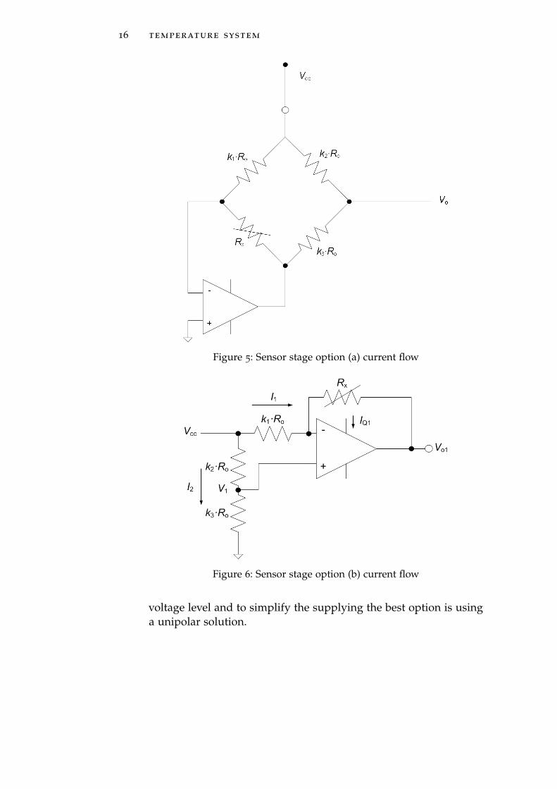
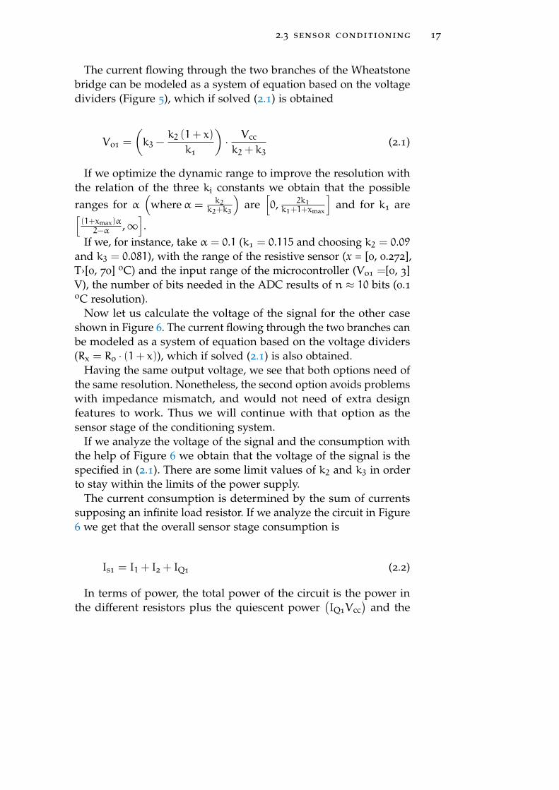
There are two typical circuits for conditioning through pseudo-bridges[56], unipolar as can be seen in Figure 5 and bipolar in Figure6. On a first sight we can see that Figure 6 will not have mismatchproblems since its output is regulated by an operational amplifier(OA). Still both circuits are analyzed in order to see which will needa lower ADC resolution.
A Pt1000 sensor , with a nominal resistance of Ro = 1 kΩ, besides,and a range of Rx = [1− 1.272] kΩ are considered. In this stage, thevariables that will determine the trade-off between the consumptionand the effective resolution are ki. Let us calculate first the voltageof the signal for the option in Figure 5.
This option would need a reference instead of ground in thepositive input of the amplifier, or bipolar supplying, in order to beable to output the whole range of the sensor. Thus, to reduce the
16 temperature system
Figure 5: Sensor stage option (a) current flow
Figure 6: Sensor stage option (b) current flow
voltage level and to simplify the supplying the best option is usinga unipolar solution.
2.3 sensor conditioning 17
The current flowing through the two branches of the Wheatstonebridge can be modeled as a system of equation based on the voltagedividers (Figure 5), which if solved (2.1) is obtained
Vo1 =
(k3 −
k2 (1+ x)
k1
)· Vcc
k2 + k3(2.1)
If we optimize the dynamic range to improve the resolution withthe relation of the three ki constants we obtain that the possibleranges for α
(whereα = k2
k2+k3
)are
[0, 2k1k1+1+xmax
]and for k1 are[
(1+xmax)α2−α ,∞].
If we, for instance, take α = 0.1 (k1 = 0.115 and choosing k2 = 0.09and k3 = 0.081), with the range of the resistive sensor (x = [0, 0.272],T›[0, 70] oC) and the input range of the microcontroller (Vo1 =[0, 3]V), the number of bits needed in the ADC results of n ≈ 10 bits (0.1oC resolution).
Now let us calculate the voltage of the signal for the other caseshown in Figure 6. The current flowing through the two branches canbe modeled as a system of equation based on the voltage dividers(Rx = Ro · (1+ x)), which if solved (2.1) is also obtained.
Having the same output voltage, we see that both options need ofthe same resolution. Nonetheless, the second option avoids problemswith impedance mismatch, and would not need of extra designfeatures to work. Thus we will continue with that option as thesensor stage of the conditioning system.
If we analyze the voltage of the signal and the consumption withthe help of Figure 6 we obtain that the voltage of the signal is thespecified in (2.1). There are some limit values of k2 and k3 in orderto stay within the limits of the power supply.
The current consumption is determined by the sum of currentssupposing an infinite load resistor. If we analyze the circuit in Figure6 we get that the overall sensor stage consumption is
Is1 = I1 + I2 + IQ1 (2.2)
In terms of power, the total power of the circuit is the power inthe different resistors plus the quiescent power
(IQ1Vcc
)and the
18 temperature system
internal power depending on the amplification[57]. The resultingpower consumption in Figure 6 is
Ps1 =V2ccRo
(1
k1
(1−
k3k2 + k3
)+
1
k2 + k3
)+ IQ1Vcc (2.3)
As we can see in equation (2.3), k3k2+k3
needs to be smaller than 1
in order to fulfill the equation.As for the noise, when added it is possible to see that the predom-
inant noises are the thermal and flicker noise and all the rest arenegligible[57].
With that in mind, in Figure 6 the voltage and current thermalnoise sources are identified. A method to determine the circuit gainfor each noise source is to replace them by a conventional voltage orcurrent source and calculate the corresponding gain [52].
We get the equation defining the output voltage in Figure 6 takinginto account the voltage and current thermal noise sources, whichshows the respective gain for each voltage and current source. There-fore, the Power Spectral Density (PSD) of the output voltage noisewill be
e2no1=
[(1+ k1k1
)2(k3
k2 + k3
)2(k2 + k3) +
1
k1+ 1
]e2to
+
(1+ k1k1
)2e2n1
+
[(1+ k1k1
)(k2k3k2 + k3
)+ 1
]2R2o · i2n1
(2.4)
If the output mean-square voltage noise when measured with adevice whose bandwidth goes from fL to fHis [56]
E2no1=
∫ fHfL
e2no (f)df (2.5)
and if the flicker noise for the respective frequency dependence ofen and in for common operational amplifiers[57] is
e2n (f) = e2no ·(fce ln
(fHfL
)+ (fH − fL)
)(2.6)
i2n (f) = i2no ·(fce ln
(fHfL
)+ (fH − fL)
)(2.7)
2.3 sensor conditioning 19
we can finally obtain from (2.4) and with (2.5), (2.6) and (2.7)
E2no1=
[(1+ k1k1
)2(k3
k2 + k3
)2(k2 + k3) +
1
k1+ 1
]e2to
· (fH − fL) +
(1+ k1k1
)2e2no ·
(fce ln
(fHfL
)+ (fH − fL)
)+
[(1+ k1k1
)(k2k3k2 + k3
)+ 1
]2R2o · i2no ·
(fce ln
(fHfL
)+ (fH − fL)
)(2.8)
filtering stage A first order low-pass filter is considered. Letus see the voltage of the signal and the consumption considering aresistance of the filter Rf and a capacitance of the filter C.
In this case voltage Vo2 in steady state will equal the voltage inthe input Vo1.
As for the consumption, if the capacitor is initially discharged, thevoltage in this stage will be function of the time of charge. Therefore,the current evolution is represented by (2.9) as
If =Vo1
Rf·(1− e−t/fi
)· u (t) (2.9)
If we consider the filtering time lτ = 6.9τ or lτ = 9.2τ, the effectivenumber of bits results 10 and 14 bits respectively and hence theaverage consumption is
If,a =1
lτ
∫ lτ0
Vo1
Rf· e−t/fidτ =
Vo1C
l
(1− e−l
)(2.10)
Knowing that fH = 12πRC and considering that the values of l are
really high (an integration time of 6.9τ or higher to decrease thetime in active), making e−l ≈ 0, then
If,a =Vo1
l · 2π · fH · Rf(2.11)
The power consumption similarly is
Pf,a =1
lτ
∫ lτ0
2V2o1
Rf· e−2t/fidτ ≈ V2o1
l · Rf(2.12)
20 temperature system
And for noise, since there is no active components and there is onlyone resistor, the influence of noise for the filtering stage will add thethermal noise of that resistor, finally obtain the output mean-squarevoltage noise with (2.5), (2.6) and (2.7)
E2no2= E2no1
+ e2tf (fH − fL) (2.13)
processing and adc stage We will not consider the activeprocessing stage because it is very variable depending of the com-piler and the program, and because it is common for all the condi-tioning systems and, thus, not a differential point. The case of theADC is different since there are conditioning systems not using it.
The analog-to-digital conversion is characterized by three time in-tervals: synchronism time (tsync), sampling time (ts) and conversiontime (tc). During these intervals the ADC is actively consuming.
As for the influence of noise for the ADC stage we will considerthe Quantization noise, which is due to the finite resolution of theADC, and is an unavoidable imperfection in all types of ADC. TheADC thermal noise is negligible with an order of 10−18. Also, onehas to be careful when choosing an ADC due to the error comingfrom non-linearities, gain error, etc.
The magnitude of the quantization error at the sampling instantis between zero and half one LSB. In the general case, the origi-nal signal is much larger than one LSB. When this happens, thequantization error is not correlated with the signal, and has a uni-form distribution. Its RMS value is the standard deviation of thisdistribution, given by[58].
eQ =Q√12
(2.14)
where
Q =VFS
2n(2.15)
VFS is the full scale voltage and n is the number of bits of theADC.
Therefore, the output mean-square voltage noise is
E2Q =V2FS12 · 22n
(2.16)
2.3 sensor conditioning 21
overall average consumption and effective resolution
In order to calculate the energy consumption of the overall condi-tioning system (Ea), an average depending on the monitoring rate isrealized
Es,a = t1Ps1 + tfPf,a + tADCPADC + tuC,sleepPuC,sleep (2.17)
where tT is the monitoring rate, tf is the time the filtering stage isactive
tf = l · τ (2.18)
tADC is the time the ADC is active in the worst case
tADC = tsinc + ts + tc (2.19)
tuC,sleep is the time the microcontroller is in sleep mode, which isthe rest of the time
tuC,sleep = tT − t1 (2.20)
and t1 is the time the sensor stage is active, which equals to thetime spent on the filtering and amplification stage (the 2 additionalclocks are the intervals between the active cycles of the ADC)
t1 = tf + tADC + 2 · TSCLK (2.21)
As for the resolution, we will define it as the effective number ofbits after the signal has been digitized
ENOB =
10 log(V2o2
E2noT
)− 1.76
6.02(2.22)
where E2noT is the total output mean-square voltage noise
E2noT = E2no2+ E2Q (2.23)
22 temperature system
With equations (2.17) and (2.22) we will study the consumptionand effective resolution of a classic conditioning system in section2.3.1.
Time conditioning (Direct sensor-to-microcontroller interface)
This conditioning consists on the time measure of the charge anddischarge of a capacitor through the resistive sensor, using the digitalinputs and outputs of an MCU, whilst capturing the time with acounter. This time will depend directly on the resistance value ofthe sensor.
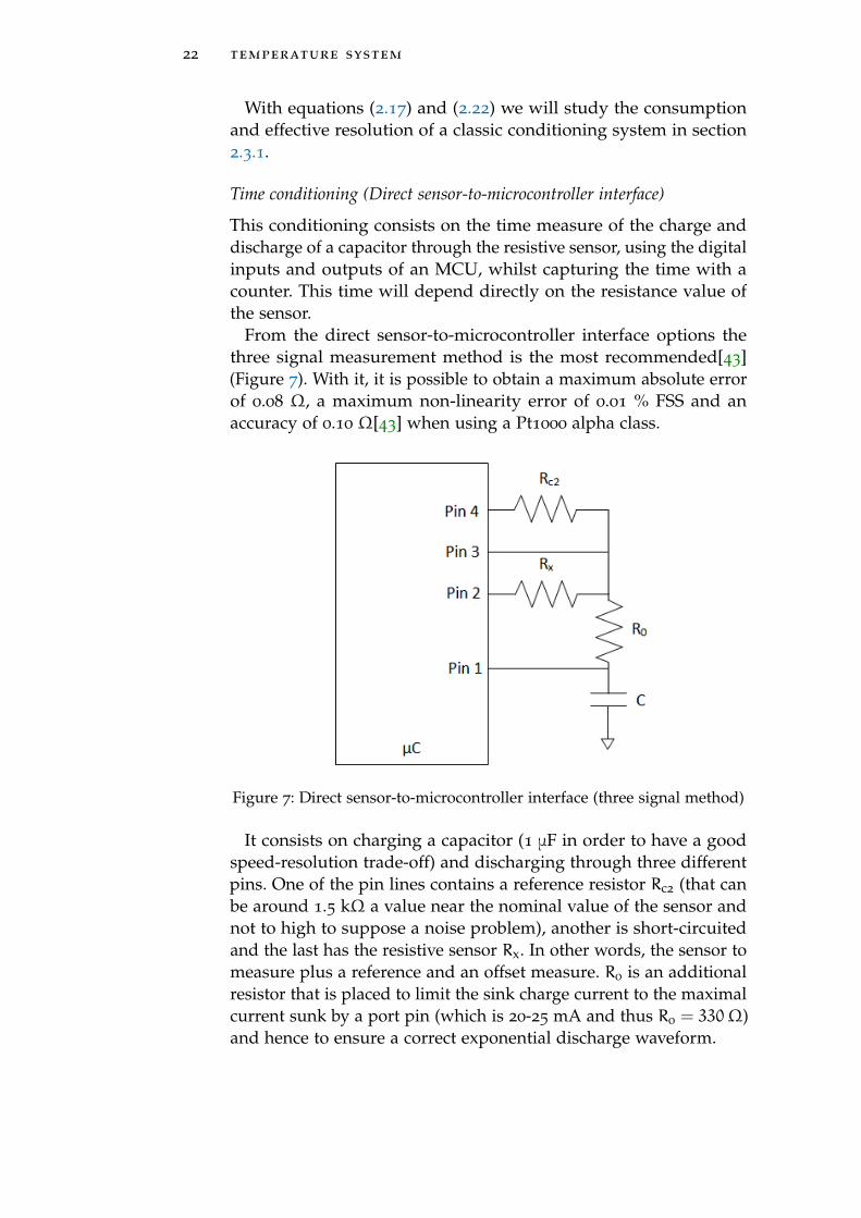
From the direct sensor-to-microcontroller interface options thethree signal measurement method is the most recommended[43](Figure 7). With it, it is possible to obtain a maximum absolute errorof 0.08 Ω, a maximum non-linearity error of 0.01 % FSS and anaccuracy of 0.10 Ω[43] when using a Pt1000 alpha class.
Figure 7: Direct sensor-to-microcontroller interface (three signal method)
It consists on charging a capacitor (1 μF in order to have a goodspeed-resolution trade-off) and discharging through three differentpins. One of the pin lines contains a reference resistor Rc2 (that canbe around 1.5 kΩ a value near the nominal value of the sensor andnot to high to suppose a noise problem), another is short-circuitedand the last has the resistive sensor Rx. In other words, the sensor tomeasure plus a reference and an offset measure. R0 is an additionalresistor that is placed to limit the sink charge current to the maximalcurrent sunk by a port pin (which is 20-25 mA and thus R0 = 330Ω)and hence to ensure a correct exponential discharge waveform.
2.3 sensor conditioning 23
From each discharge the time it lasts is measured, and witheach time the resistance value of the sensor can be calculated with(2.24)[59]
Rx = R0 ·Nx −Nc1
Nc2 −Nc1
(2.24)
where Nx is the time counter of discharge through the resistivesensor, Nc1 is the time counter of discharge through the short-circuitand Nc2 is the time counter of discharge through the resistor Rc2.
overall consumption The overall consumption of this sys-tem only depends on the operation of the microcontroller and thecharges and discharges of the three signal measurement method. Asin the previous system we suppose that the microcontroller is sleep-ing most of the time except when measuring. Also while chargingand discharging the MCU is sleeping until the trigger is activated.Therefore the overall energy consumption as an averaging of theconsumption is
Es,a = tuC,activePuC,active + tRc2PRc2
+ tRscPRsc + tRxPRx
+ tuC,sleepPuC,sleep (2.25)
where tuC,active is the time the microcontroller is active, PuC,activeis the power consumption of the microcontroller when active, tRc2
is the discharge time through Rc2, PRc2is the power consumption
of the discharge through Rc2, tRscis the discharge time through theshort-circuit, PRscis power consumption of the discharge throughthe short-circuit, tRx is the discharge time through the sensor, PRx isthe power consumption of the discharge through the sensor, tuC,sleepis the time the microcontroller is asleep and PuC,sleep is the powerconsumption when the microcontroller is asleep.
effective resolution The effective resolution of the threesignal measurement method can be simplified to (2.26) since Rx Rsc and Rc2 Rsc[60]
u (R∗x)
R∗x= ur,0 ·
√2 (2.26)
24 temperature system
where ur,0 is the relative standard uncertainty of the dischargingtime measurement, which remains constant as in (2.27)
ur,0 =u (Nx)
Nx=u (Nc1)
Nc1
=u (Nc2)
Nc2
(2.27)
Since the value of the discharge measurement cannot be consid-ered small, the Slew Rate (SR) at the trigger point is small andhence the effects of the trigger noise predominate over those ofquantization[21], therefore the relative standard uncertainty of thedischarging time measurement can be approximated to (2.28)
ur,0 ≈
√E2n,i + E
2n,e
(VTL − V0) · ln(V1−V0
VTL−V0
) (2.28)
where En,i is the rms voltage noise superimposed on the thresholdvoltage, En,e is the rms voltage noise superimposed on the inputsignal to be measured, VTL is the lower threshold voltage of themicrocontroller, V0 is the value to which the discharge arrives andV1 is the value from which the discharge departs.
And thus the effective number of bits (ENOB) results as (2.29)
ENOB = log2
Rmax − Rmin
Rmax
(VTL − V0) · ln(
V1−V0
VTL−V0
)√
12 ·√
E2
n,i + E2
n,e
(2.29)
where Rmax and Rmin are the maximal and minimal values of theresistive sensor.
If a reduction of the trigger noise is realized (similar to filtering)by averaging several measures (above 100 measures[43]) then quan-tization noise predominates and the relative standard uncertaintycan be approximated to (2.30)
ur,0 ≈T s
√12τ · ln
(V1−V0
VTL−V0
) (2.30)
where T s is the time-base of the digital timer.
2.3 sensor conditioning 25
And thus the ENOB results as (2.31)
ENOB = log2
(T0,max − T0,min
Ts
)(2.31)
where T0,min and T0,max are respectively the minimal and maximaldischarging times to be measured.
Theoretical results and discussion
First, the energy consumption and the effective number of bits arecalculated for the amplitude conditioning and compared. Frequen-cies from 0.47 Hz to 20 Hz are considered; most of sensors work atlow frequencies and the selected 16 bit ADC samples at 38.15 Hzand hence 20 Hz is more than enough. The 24 bit ADC cannot beused due to sampling time issues (the sampling frequency is 0.30 Hzand as such cannot sample signals between the specified frequencyrange) and also the consumption would be increased dramaticallyto achieve an extra bit of resolution.
In order to emulate a real example, a voltage supply of Vcc = 3V,a monitoring rate of 1 sample/h and a temperature of 273 K aresupposed. Optimum devices are chosen in order to minimize theireffect in the consumption and in the noise:
• A low power AD8500 amplifier is used, with a quiescentcurrent of IQ1 = 1.5 μA, a voltage noise density of eno =
190 nV/√
Hz and a current noise density of ino = 0.1 pA.
• The very low consumption MSP430F1232 microcontroller, withan active current of IuC,active = 580μA and a sleep mode currentof IuC,sleep = 0.5 μA. The same MCU is supposed in bothsystems (En,i = En.e 6 1.45mV, VTL = 1.65 V, f = 8 MHz).
• The AD7788/AD7789 16/24 bit ADC, with a current supply ofIADC = 75 μA for a VDD = 3.6V, and a TSCLK = 200 ns; in thecase of this device the working times are defined as tsync = tT,ts = 2
n · TSCLK and tc = 2 · tT.
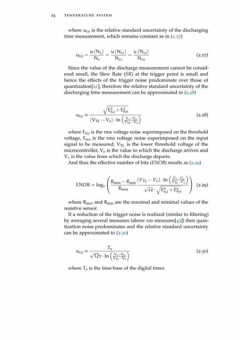
As said in the excitation stage section, α and k1 need to be as near of0 as possible. Figure 8 shows the effective number of bits in functionof the energy consumption for α = 0.1 and k2 = 0.09 and with arange of k1 from 0.1121 to 0.1414, the limit values to be within thevoltage supply range. From left to right the points of the graphequal the values of effective resolution and energy consumption forbandwidth of [20, 17.6, . . . , 0.538, 0.473] Hz.
26 temperature system
Figure 8: Energy consumption vs effective number of bits (α = 0.1). Pointsof each series are, from left to right, 20, 17.6, . . . , 0.538, 0.473 Hz.For a 16 bit ADC.
As we can see, the bigger the value of k1 the better the resolutionand the consumption. In this case Equation (2.8) is not affected byα and so it directly affects the signal amplitude of Equation (2.1)and the power consumption of Equation (2.3). Without taking a lookat the equations, this behavior may seem not logical, but there areworks that have proved the seemingly paradoxical noise behavior ofsome active circuits[61].
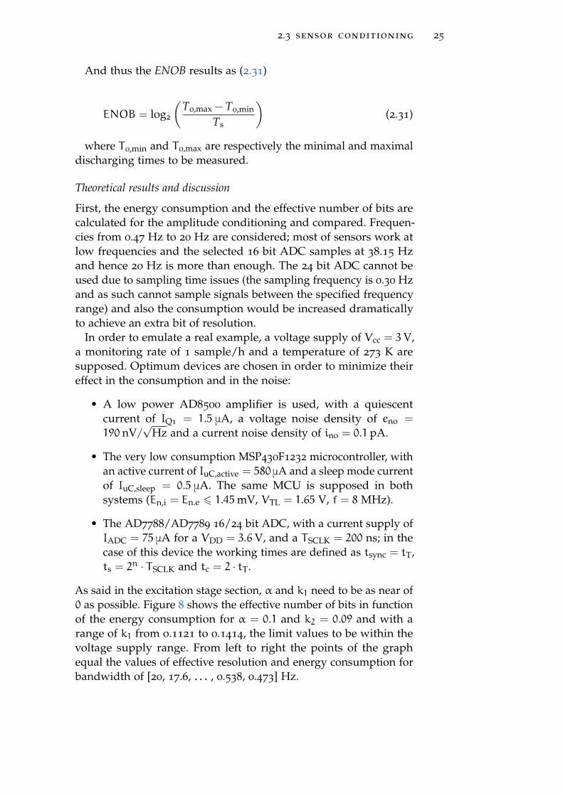
If we take a medium case in Figure 8 (k1 = 0.1185) and we modifyα within its limit values [0.0712, 0.1060] we obtain Figure 9. Thistime, the smaller the value of α the better the resolution and theconsumption, which implies that k3 must be much bigger than k2.This can be expected since if we take a look at equation 2.4 we seethat the bigger k3compared to k2 the less noise and in equation 2.3less consumption.
Figure 9: Energy consumption vs effective number of bits (k1 = 0.1185).Points of each series are, from left to right, 20, 17.6, . . . , 0.538,0.473 Hz. For a 16 bit ADC.
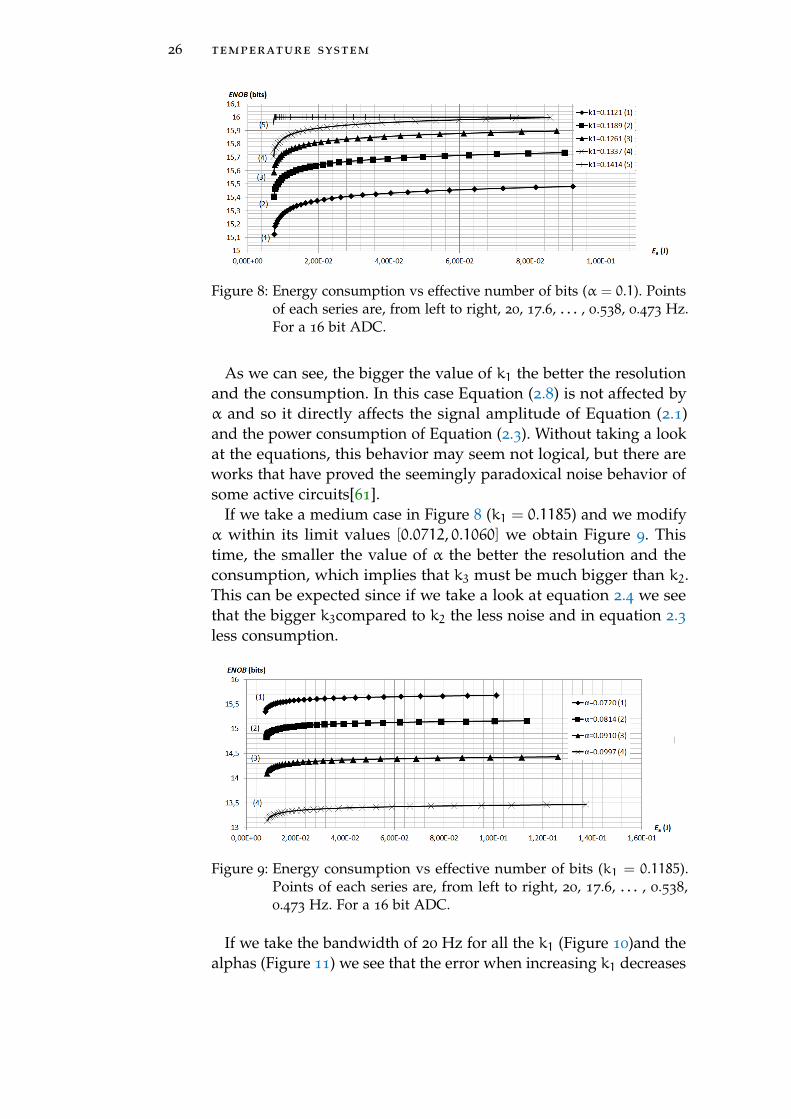
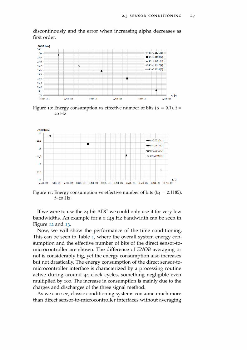
If we take the bandwidth of 20 Hz for all the k1 (Figure 10)and thealphas (Figure 11) we see that the error when increasing k1 decreases
2.3 sensor conditioning 27
discontinously and the error when increasing alpha decreases asfirst order.
Figure 10: Energy consumption vs effective number of bits (α = 0.1). f =20 Hz
Figure 11: Energy consumption vs effective number of bits (k1 = 0.1185).f=20 Hz.
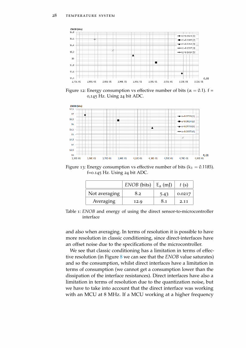
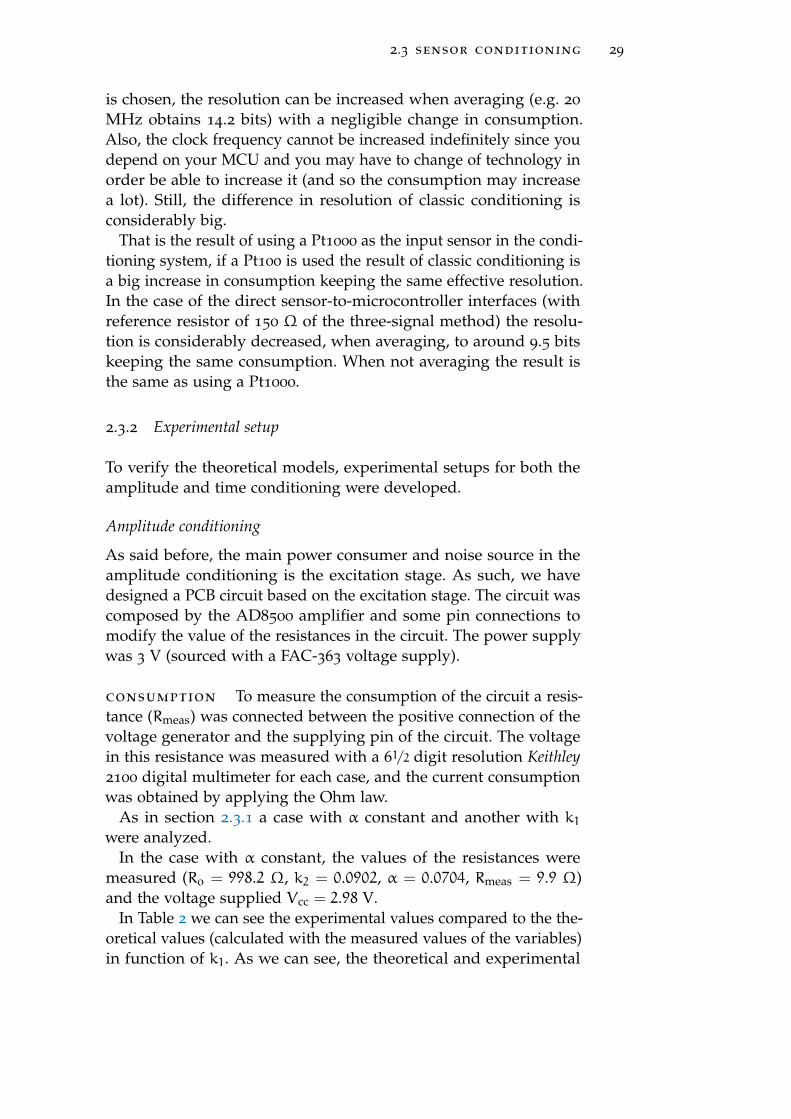
If we were to use the 24 bit ADC we could only use it for very lowbandwidths. An example for a 0.145 Hz bandwidth can be seen inFigure 12 and 13.
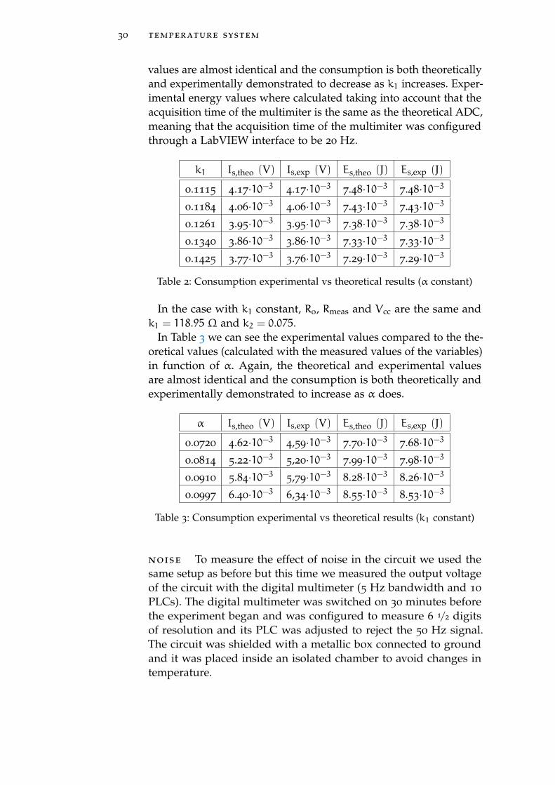
Now, we will show the performance of the time conditioning.This can be seen in Table 1, where the overall system energy con-sumption and the effective number of bits of the direct sensor-to-microcontroller are shown. The difference of ENOB averaging ornot is considerably big, yet the energy consumption also increasesbut not drastically. The energy consumption of the direct sensor-to-microcontroller interface is characterized by a processing routineactive during around 44 clock cycles, something negligible evenmultiplied by 100. The increase in consumption is mainly due to thecharges and discharges of the three signal method.
As we can see, classic conditioning systems consume much morethan direct sensor-to-microcontroller interfaces without averaging
28 temperature system
Figure 12: Energy consumption vs effective number of bits (α = 0.1). f =0,145 Hz. Using 24 bit ADC.
Figure 13: Energy consumption vs effective number of bits (k1 = 0.1185).f=0.145 Hz. Using 24 bit ADC.
ENOB (bits) Ea (mJ) t (s)
Not averaging 8.2 5.43 0.0217
Averaging 12.9 8.1 2.11
Table 1: ENOB and energy of using the direct sensor-to-microcontrollerinterface
and also when averaging. In terms of resolution it is possible to havemore resolution in classic conditioning, since direct-interfaces havean offset noise due to the specifications of the microcontroller.
We see that classic conditioning has a limitation in terms of effec-tive resolution (in Figure 8 we can see that the ENOB value saturates)and so the consumption, whilst direct interfaces have a limitation interms of consumption (we cannot get a consumption lower than thedissipation of the interface resistances). Direct interfaces have also alimitation in terms of resolution due to the quantization noise, butwe have to take into account that the direct interface was workingwith an MCU at 8 MHz. If a MCU working at a higher frequency
2.3 sensor conditioning 29
is chosen, the resolution can be increased when averaging (e.g. 20
MHz obtains 14.2 bits) with a negligible change in consumption.Also, the clock frequency cannot be increased indefinitely since youdepend on your MCU and you may have to change of technology inorder be able to increase it (and so the consumption may increasea lot). Still, the difference in resolution of classic conditioning isconsiderably big.
That is the result of using a Pt1000 as the input sensor in the condi-tioning system, if a Pt100 is used the result of classic conditioning isa big increase in consumption keeping the same effective resolution.In the case of the direct sensor-to-microcontroller interfaces (withreference resistor of 150 Ω of the three-signal method) the resolu-tion is considerably decreased, when averaging, to around 9.5 bitskeeping the same consumption. When not averaging the result isthe same as using a Pt1000.
2.3.2 Experimental setup
To verify the theoretical models, experimental setups for both theamplitude and time conditioning were developed.
Amplitude conditioning
As said before, the main power consumer and noise source in theamplitude conditioning is the excitation stage. As such, we havedesigned a PCB circuit based on the excitation stage. The circuit wascomposed by the AD8500 amplifier and some pin connections tomodify the value of the resistances in the circuit. The power supplywas 3 V (sourced with a FAC-363 voltage supply).
consumption To measure the consumption of the circuit a resis-tance (Rmeas) was connected between the positive connection of thevoltage generator and the supplying pin of the circuit. The voltagein this resistance was measured with a 61/2 digit resolution Keithley2100 digital multimeter for each case, and the current consumptionwas obtained by applying the Ohm law.
As in section 2.3.1 a case with α constant and another with k1were analyzed.
In the case with α constant, the values of the resistances weremeasured (Ro = 998.2 Ω, k2 = 0.0902, α = 0.0704, Rmeas = 9.9 Ω)and the voltage supplied Vcc = 2.98 V.
In Table 2 we can see the experimental values compared to the the-oretical values (calculated with the measured values of the variables)in function of k1. As we can see, the theoretical and experimental
30 temperature system
values are almost identical and the consumption is both theoreticallyand experimentally demonstrated to decrease as k1 increases. Exper-imental energy values where calculated taking into account that theacquisition time of the multimiter is the same as the theoretical ADC,meaning that the acquisition time of the multimiter was configuredthrough a LabVIEW interface to be 20 Hz.
k1 Is,theo (V) Is,exp (V) Es,theo (J) Es,exp (J)
0.1115 4.17·10−3 4.17·10−3 7.48·10−3 7.48·10−3
0.1184 4.06·10−3 4.06·10−3 7.43·10−3 7.43·10−3
0.1261 3.95·10−3 3.95·10−3 7.38·10−3 7.38·10−3
0.1340 3.86·10−3 3.86·10−3 7.33·10−3 7.33·10−3
0.1425 3.77·10−3 3.76·10−3 7.29·10−3 7.29·10−3
Table 2: Consumption experimental vs theoretical results (α constant)
In the case with k1 constant, Ro, Rmeas and Vcc are the same andk1 = 118.95 Ω and k2 = 0.075.
In Table 3 we can see the experimental values compared to the the-oretical values (calculated with the measured values of the variables)in function of α. Again, the theoretical and experimental valuesare almost identical and the consumption is both theoretically andexperimentally demonstrated to increase as α does.
α Is,theo (V) Is,exp (V) Es,theo (J) Es,exp (J)
0.0720 4.62·10−3 4,59·10−3 7.70·10−3 7.68·10−3
0.0814 5.22·10−3 5,20·10−3 7.99·10−3 7.98·10−3
0.0910 5.84·10−3 5,79·10−3 8.28·10−3 8.26·10−3
0.0997 6.40·10−3 6,34·10−3 8.55·10−3 8.53·10−3
Table 3: Consumption experimental vs theoretical results (k1 constant)
noise To measure the effect of noise in the circuit we used thesame setup as before but this time we measured the output voltageof the circuit with the digital multimeter (5 Hz bandwidth and 10
PLCs). The digital multimeter was switched on 30 minutes beforethe experiment began and was configured to measure 6 1/2 digitsof resolution and its PLC was adjusted to reject the 50 Hz signal.The circuit was shielded with a metallic box connected to groundand it was placed inside an isolated chamber to avoid changes intemperature.
2.3 sensor conditioning 31
Both the k1 and α modification cases were tested with the samecharacteristics as in the previous experiment. One could think thatthese are really small values for resistances, but as explained insection 2.3.1 k1 and α need to be within certain margins to fulfill thedynamic range. Morevore, given that Ro is equal to 1000 Ω, as perthe Pt1000 sensor used, the values of the rest of resistances are verysmall.
The output voltage was captured during 15 minutes at a 10 Hzrate. From the resulting signal we obtained the mean and standarddeviation, and with those we could obtain subsequently the ENOBwith equation 2.22 using the mean as the power of the signal andthe deviation as the power of the noise.
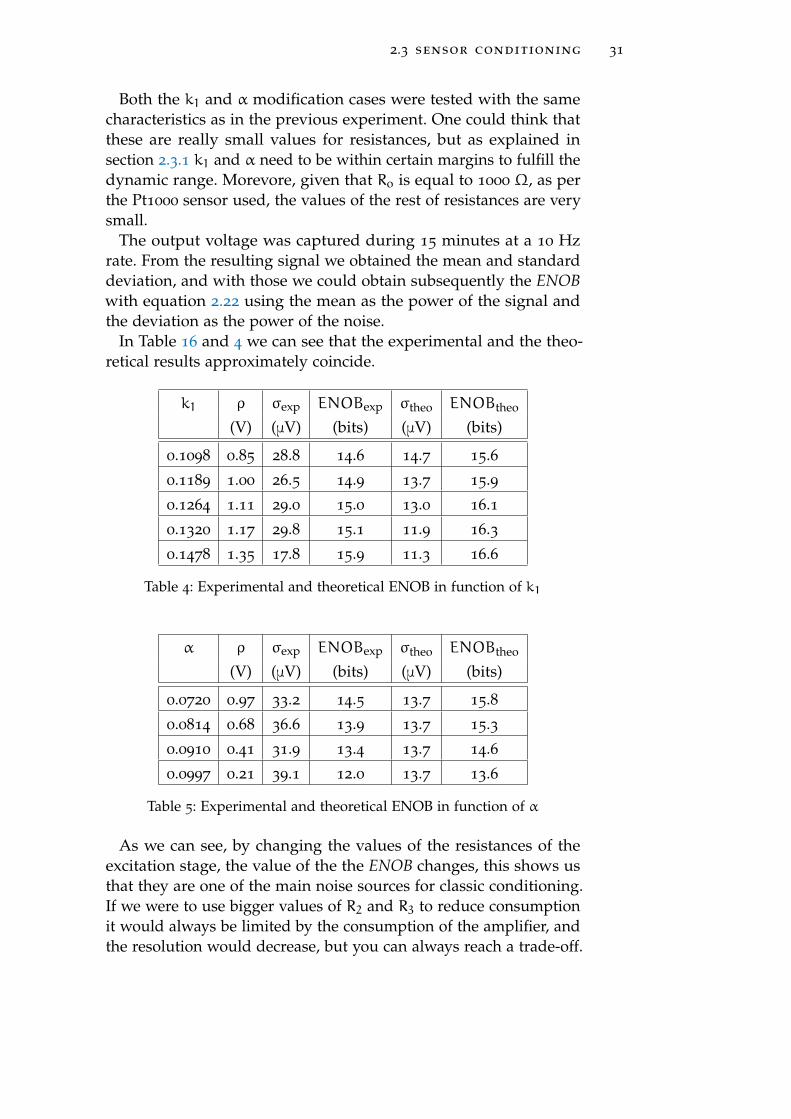
In Table 16 and 4 we can see that the experimental and the theo-retical results approximately coincide.
k1 ρ σexp ENOBexp σtheo ENOBtheo
(V) (μV) (bits) (μV) (bits)
0.1098 0.85 28.8 14.6 14.7 15.6
0.1189 1.00 26.5 14.9 13.7 15.9
0.1264 1.11 29.0 15.0 13.0 16.1
0.1320 1.17 29.8 15.1 11.9 16.3
0.1478 1.35 17.8 15.9 11.3 16.6
Table 4: Experimental and theoretical ENOB in function of k1
α ρ σexp ENOBexp σtheo ENOBtheo
(V) (μV) (bits) (μV) (bits)
0.0720 0.97 33.2 14.5 13.7 15.8
0.0814 0.68 36.6 13.9 13.7 15.3
0.0910 0.41 31.9 13.4 13.7 14.6
0.0997 0.21 39.1 12.0 13.7 13.6
Table 5: Experimental and theoretical ENOB in function of α
As we can see, by changing the values of the resistances of theexcitation stage, the value of the the ENOB changes, this shows usthat they are one of the main noise sources for classic conditioning.If we were to use bigger values of R2 and R3 to reduce consumptionit would always be limited by the consumption of the amplifier, andthe resolution would decrease, but you can always reach a trade-off.
32 temperature system
In Table 5 we see that the theoretical noise is constant and in Table4 is not; this shows that k1 greatly affects the noise proportionally.
We can see that the experimental value is slightly smaller thanthe theoretical one, this is mainly due to the variation on noise onthe operational amplifier. There is no fixed variation of the typi-cal voltage noise and the maximum voltage noise for operationalamplifiers. However, we can find many examples that show thatthe maximum voltage noise of commercial operational amplifierscan be more than twice the typical (e.g. OPA2111AM, OPA2111BM,OPA2111SM, OPA37G, AD795JN/JR, AD795K).
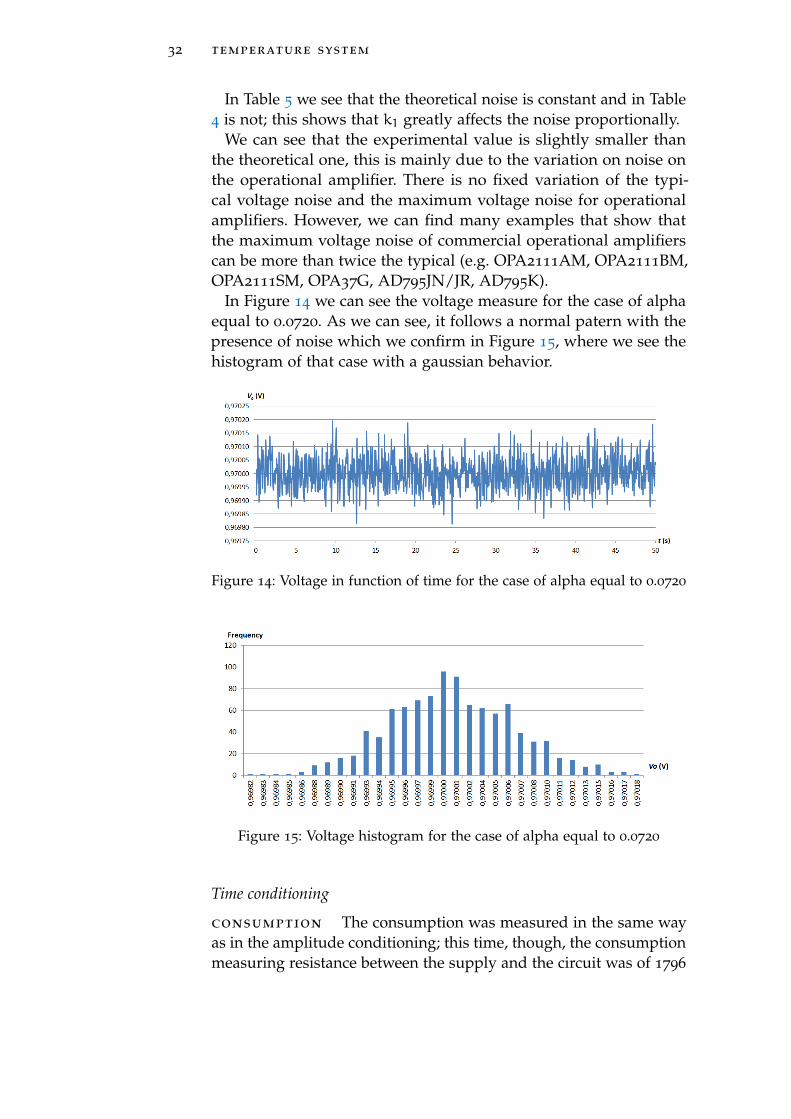
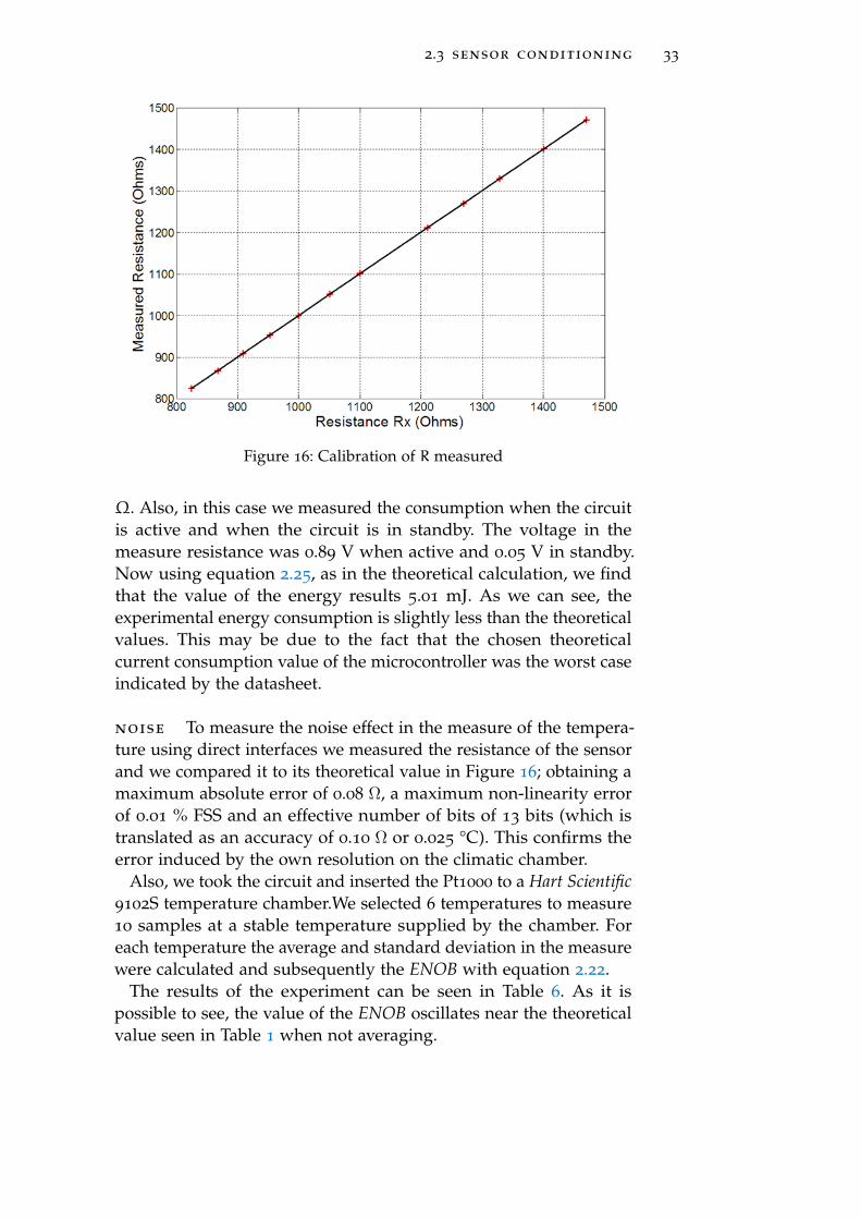
In Figure 14 we can see the voltage measure for the case of alphaequal to 0.0720. As we can see, it follows a normal patern with thepresence of noise which we confirm in Figure 15, where we see thehistogram of that case with a gaussian behavior.
Figure 14: Voltage in function of time for the case of alpha equal to 0.0720
Figure 15: Voltage histogram for the case of alpha equal to 0.0720
Time conditioning
consumption The consumption was measured in the same wayas in the amplitude conditioning; this time, though, the consumptionmeasuring resistance between the supply and the circuit was of 1796
2.3 sensor conditioning 33
Figure 16: Calibration of R measured
Ω. Also, in this case we measured the consumption when the circuitis active and when the circuit is in standby. The voltage in themeasure resistance was 0.89 V when active and 0.05 V in standby.Now using equation 2.25, as in the theoretical calculation, we findthat the value of the energy results 5.01 mJ. As we can see, theexperimental energy consumption is slightly less than the theoreticalvalues. This may be due to the fact that the chosen theoreticalcurrent consumption value of the microcontroller was the worst caseindicated by the datasheet.
noise To measure the noise effect in the measure of the tempera-ture using direct interfaces we measured the resistance of the sensorand we compared it to its theoretical value in Figure 16; obtaining amaximum absolute error of 0.08 Ω, a maximum non-linearity errorof 0.01 % FSS and an effective number of bits of 13 bits (which istranslated as an accuracy of 0.10 Ω or 0.025 °C). This confirms theerror induced by the own resolution on the climatic chamber.
Also, we took the circuit and inserted the Pt1000 to a Hart Scientific9102S temperature chamber.We selected 6 temperatures to measure10 samples at a stable temperature supplied by the chamber. Foreach temperature the average and standard deviation in the measurewere calculated and subsequently the ENOB with equation 2.22.
The results of the experiment can be seen in Table 6. As it ispossible to see, the value of the ENOB oscillates near the theoreticalvalue seen in Table 1 when not averaging.
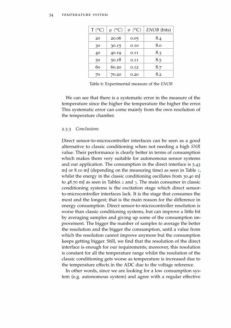
34 temperature system
T (oC) ρ (oC) σ (oC) ENOB (bits)
20 20.06 0.05 8.4
30 30.15 0.10 8.0
40 40.19 0.11 8.3
50 50.18 0.11 8.5
60 60.20 0.12 8.7
70 70.20 0.20 8.2
Table 6: Experimental measure of the ENOB
We can see that there is a systematic error in the measure of thetemperature since the higher the temperature the higher the error.This systematic error can come mainly from the own resolution ofthe temperature chamber.
2.3.3 Conclusions
Direct sensor-to-microcontroller interfaces can be seen as a goodalternative to classic conditioning when not needing a high SNRvalue. Their performance is clearly better in terms of consumptionwhich makes them very suitable for autonomous sensor systemsand our application. The consumption in the direct interface is 5.43
mJ or 8.10 mJ (depending on the measuring time) as seen in Table 1,whilst the energy in the classic conditioning oscillates from 30.40 mJto 48.70 mJ as seen in Tables 2 and 3. The main consumer in classicconditioning systems is the excitation stage which direct sensor-to-microcontroller interfaces lack. It is the stage that consumes themost and the longest; that is the main reason for the difference inenergy consumption. Direct sensor-to-microcontroller resolution isworse than classic conditioning systems, but can improve a little bitby averaging samples and giving up some of the consumption im-provement. The bigger the number of samples to average the betterthe resolution and the bigger the consumption, until a value fromwhich the resolution cannot improve anymore but the consumptionkeeps getting bigger. Still, we find that the resolution of the directinterface is enough for our requirements; moreover, this resolutionis constant for all the temperature range whilst the resolution of theclassic conditioning gets worse as temperature is increased due tothe temperature effects in the ADC due to the voltage reference.
In other words, since we are looking for a low consumption sys-tem (e.g. autonomous system) and agree with a regular effective
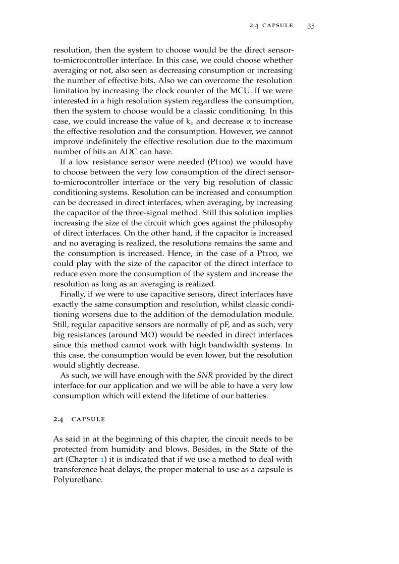
2.4 capsule 35
resolution, then the system to choose would be the direct sensor-to-microcontroller interface. In this case, we could choose whetheraveraging or not, also seen as decreasing consumption or increasingthe number of effective bits. Also we can overcome the resolutionlimitation by increasing the clock counter of the MCU. If we wereinterested in a high resolution system regardless the consumption,then the system to choose would be a classic conditioning. In thiscase, we could increase the value of k1 and decrease α to increasethe effective resolution and the consumption. However, we cannotimprove indefinitely the effective resolution due to the maximumnumber of bits an ADC can have.
If a low resistance sensor were needed (Pt100) we would haveto choose between the very low consumption of the direct sensor-to-microcontroller interface or the very big resolution of classicconditioning systems. Resolution can be increased and consumptioncan be decreased in direct interfaces, when averaging, by increasingthe capacitor of the three-signal method. Still this solution impliesincreasing the size of the circuit which goes against the philosophyof direct interfaces. On the other hand, if the capacitor is increasedand no averaging is realized, the resolutions remains the same andthe consumption is increased. Hence, in the case of a Pt100, wecould play with the size of the capacitor of the direct interface toreduce even more the consumption of the system and increase theresolution as long as an averaging is realized.
Finally, if we were to use capacitive sensors, direct interfaces haveexactly the same consumption and resolution, whilst classic condi-tioning worsens due to the addition of the demodulation module.Still, regular capacitive sensors are normally of pF, and as such, verybig resistances (around MΩ) would be needed in direct interfacessince this method cannot work with high bandwidth systems. Inthis case, the consumption would be even lower, but the resolutionwould slightly decrease.
As such, we will have enough with the SNR provided by the directinterface for our application and we will be able to have a very lowconsumption which will extend the lifetime of our batteries.
2.4 capsule
As said in at the beginning of this chapter, the circuit needs to beprotected from humidity and blows. Besides, in the State of theart (Chapter 1) it is indicated that if we use a method to deal withtransference heat delays, the proper material to use as a capsule isPolyurethane.
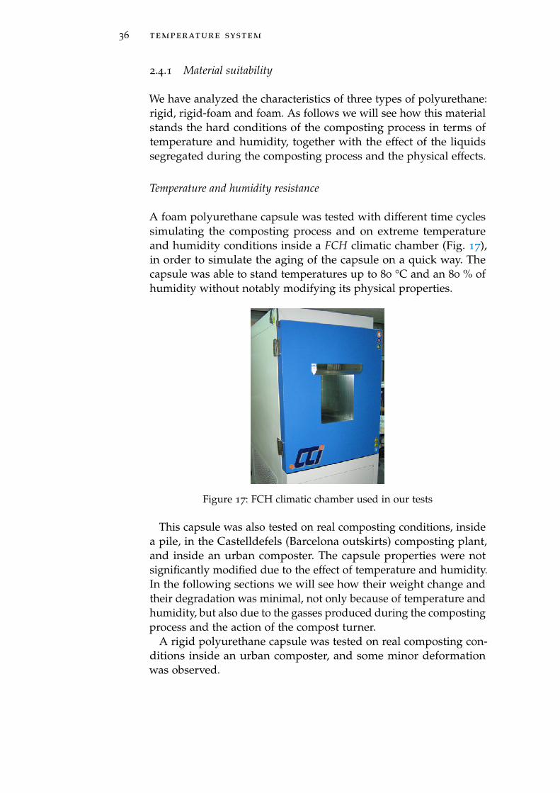
36 temperature system
2.4.1 Material suitability
We have analyzed the characteristics of three types of polyurethane:rigid, rigid-foam and foam. As follows we will see how this materialstands the hard conditions of the composting process in terms oftemperature and humidity, together with the effect of the liquidssegregated during the composting process and the physical effects.
Temperature and humidity resistance
A foam polyurethane capsule was tested with different time cyclessimulating the composting process and on extreme temperatureand humidity conditions inside a FCH climatic chamber (Fig. 17),in order to simulate the aging of the capsule on a quick way. Thecapsule was able to stand temperatures up to 80 °C and an 80 % ofhumidity without notably modifying its physical properties.
Figure 17: FCH climatic chamber used in our tests
This capsule was also tested on real composting conditions, insidea pile, in the Castelldefels (Barcelona outskirts) composting plant,and inside an urban composter. The capsule properties were notsignificantly modified due to the effect of temperature and humidity.In the following sections we will see how their weight change andtheir degradation was minimal, not only because of temperature andhumidity, but also due to the gasses produced during the compostingprocess and the action of the compost turner.
A rigid polyurethane capsule was tested on real composting con-ditions inside an urban composter, and some minor deformationwas observed.
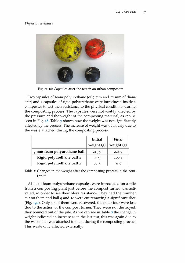
2.4 capsule 37
Physical resistance
Figure 18: Capsules after the test in an urban composter
Two capsules of foam polyurethane (of 9 mm and 12 mm of diam-eter) and 2 capsules of rigid polyurethane were introduced inside acomposter to test their resistance to the physical conditions duringthe composting process. The capsules were not visibly affected bythe pressure and the weight of the composting material, as can beseen in Fig. 18. Table 7 shows how the weight was not significantlyaffected by the process. The increase of weight was obviously due tothe waste attached during the composting process.
Initial Finalweight (g) weight (g)
9 mm foam polyurethane ball 215.7 224.9
Rigid polyurethane ball 1 95.9 100.8
Rigid polyurethane ball 2 88.5 91.0
Table 7: Changes in the weight after the composting process in the com-poster
Also, 10 foam polyurethane capsules were introduced on a pilefrom a composting plant just before the compost turner was acti-vated, in order to see their blow resistance. They had the numbercut on them and ball 9 and 10 were cut removing a significant slice(Fig. 19a). Only six of them were recovered, the other four were lostdue to the action of the compost turner. They were not destroyed;they bounced out of the pile. As we can see in Table 8 the change inweight indicated an increase as in the last test, this was again due tothe waste that was attached to them during the composting process.This waste only affected externally.
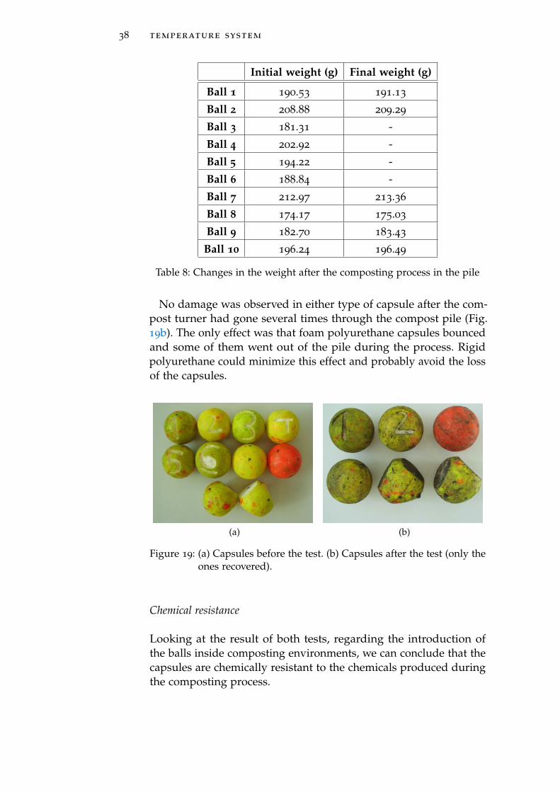
38 temperature system
Initial weight (g) Final weight (g)
Ball 1 190.53 191.13
Ball 2 208.88 209.29
Ball 3 181.31 -
Ball 4 202.92 -
Ball 5 194.22 -
Ball 6 188.84 -
Ball 7 212.97 213.36
Ball 8 174.17 175.03
Ball 9 182.70 183.43
Ball 10 196.24 196.49
Table 8: Changes in the weight after the composting process in the pile
No damage was observed in either type of capsule after the com-post turner had gone several times through the compost pile (Fig.19b). The only effect was that foam polyurethane capsules bouncedand some of them went out of the pile during the process. Rigidpolyurethane could minimize this effect and probably avoid the lossof the capsules.
(a) (b)
Figure 19: (a) Capsules before the test. (b) Capsules after the test (only theones recovered).
Chemical resistance
Looking at the result of both tests, regarding the introduction ofthe balls inside composting environments, we can conclude that thecapsules are chemically resistant to the chemicals produced duringthe composting process.
2.4 capsule 39
2.4.2 Material influence on the temperature sensor system
It is clear that the material stands the conditions of the compostingprocess. Now we will see how the material influences into the com-posting process and into the operation of the temperature sensorsystem.
As said in the first section, polyurethane delays the thermal radia-tion and thus the measure of temperature changes can be affectedfrom the inside of a polyurethane capsule. We will quantify thisdelay and will propose a solution to deal with it.
Theoretical calculation
In order to verify the validity of our experimental results we need tocompare to the theoretical calculation.
The heat transference time (∆t) from the environment at a tem-perature (T f) to a body with a volume defined by an area (A) and awidth (x) (plain surface) at another temperature (To) comes definedby[62]
∆t =∆Q · xA ·∆T ·K
(2.32)
where K is the body material conductivity, ∆T is the temperaturechange T f − To, and ∆Q is the thermal energy change Qf −Qowhichcomes from
Q = Ea · #atoms (2.33)
where Ea is the average kinetic energy per atom defined as
Ea =3
2· k · T (2.34)
where k is the Boltzmann constant which is 1.3806504 · 10−23 J/K.And the number of atoms of the body #atoms is defined as
#atoms = m ·Na
where m is the mass of the body and Na is the Avogadro numberof 6.02214179 · 1023 mol−1.
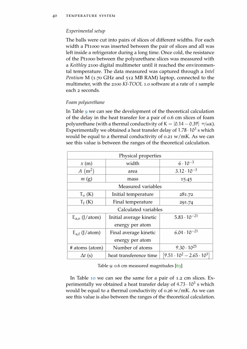
40 temperature system
Experimental setup
The balls were cut into pairs of slices of different widths. For eachwidth a Pt1000 was inserted between the pair of slices and all wasleft inside a refrigerator during a long time. Once cold, the resistanceof the Pt1000 between the polyurethane slices was measured witha Keithley 2100 digital multimeter until it reached the environmen-tal temperature. The data measured was captured through a IntelPentium M (1.70 GHz and 512 MB RAM) laptop, connected to themultimeter, with the 2100 KI-TOOL 1.0 software at a rate of 1 sampleeach 2 seconds.
Foam polyurethane
In Table 9 we can see the development of the theoretical calculationof the delay in the heat transfer for a pair of 0.6 cm slices of foampolyurethane (with a thermal conductivity of K = [0.14− 0.39] w/mK).Experimentally we obtained a heat transfer delay of 1.78 · 103 s whichwould be equal to a thermal conductivity of 0.21 w/mK. As we cansee this value is between the ranges of the theoretical calculation.
Physical properties
x (m) width 6 · 10−3
A(m2)
area 3.12 · 10−3
m (g) mass 15.45
Measured variables
To (K) Initial temperature 281.72
T f (K) Final temperature 291.74
Calculated variables
Ea,o (J/atom) Initial average kinetic 5.83 · 10−21
energy per atom
Ea,f (J/atom) Final average kinetic 6.04 · 10−21
energy per atom
# atoms (atom) Number of atoms 9.30 · 1025
∆t (s) heat transference time[9.51 · 102 − 2.65 · 103
]Table 9: 0.6 cm measured magnitudes [63]
In Table 10 we can see the same for a pair of 1.2 cm slices. Ex-perimentally we obtained a heat transfer delay of 4.73 · 103 s whichwould be equal to a thermal conductivity of 0.26 w/mK. As we cansee this value is also between the ranges of the theoretical calculation.
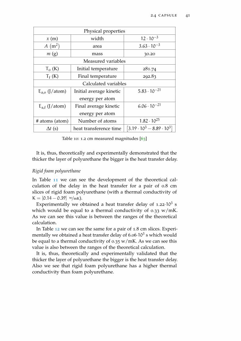
2.4 capsule 41
Physical properties
x (m) width 12 · 10−3
A(m2)
area 3.63 · 10−3
m (g) mass 30.20
Measured variables
To (K) Initial temperature 281.74
T f (K) Final temperature 292.83
Calculated variables
Ea,o (J/atom) Initial average kinetic 5.83 · 10−21
energy per atom
Ea,f (J/atom) Final average kinetic 6.06 · 10−21
energy per atom
# atoms (atom) Number of atoms 1.82 · 1025
∆t (s) heat transference time[3.19 · 103 − 8.89 · 103
]Table 10: 1.2 cm measured magnitudes [63]
It is, thus, theoretically and experimentally demonstrated that thethicker the layer of polyurethane the bigger is the heat transfer delay.
Rigid foam polyurethane
In Table 11 we can see the development of the theoretical cal-culation of the delay in the heat transfer for a pair of 0.8 cmslices of rigid foam polyurethane (with a thermal conductivity ofK = [0.14− 0.39] w/mK).
Experimentally we obtained a heat transfer delay of 1.22·103 swhich would be equal to a thermal conductivity of 0.33 w/mK.As we can see this value is between the ranges of the theoreticalcalculation.
In Table 12 we can see the same for a pair of 1.8 cm slices. Experi-mentally we obtained a heat transfer delay of 6.06·103 s which wouldbe equal to a thermal conductivity of 0.35 w/mK. As we can see thisvalue is also between the ranges of the theoretical calculation.
It is, thus, theoretically and experimentally validated that thethicker the layer of polyurethane the bigger is the heat transfer delay.Also we see that rigid foam polyurethane has a higher thermalconductivity than foam polyurethane.
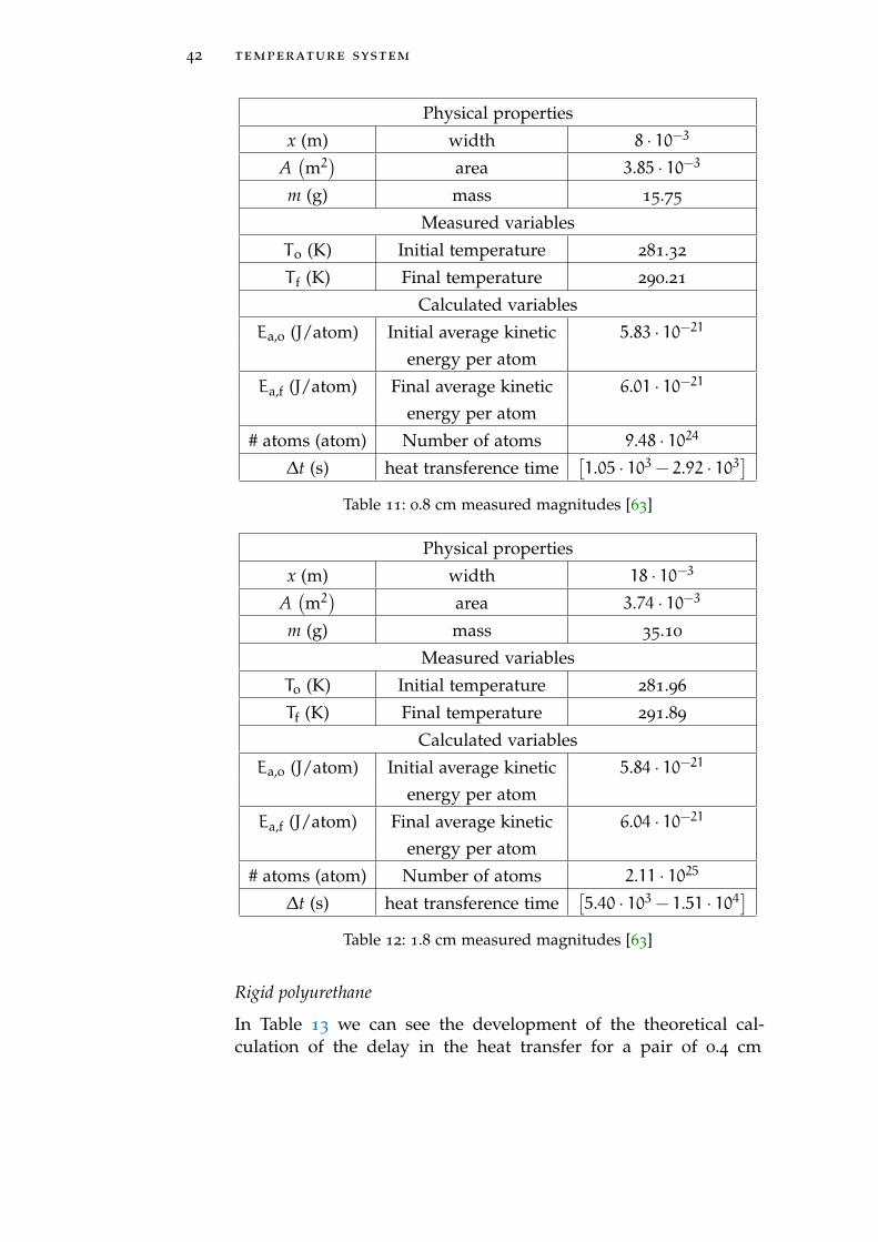
42 temperature system
Physical properties
x (m) width 8 · 10−3
A(m2)
area 3.85 · 10−3
m (g) mass 15.75
Measured variables
To (K) Initial temperature 281.32
T f (K) Final temperature 290.21
Calculated variables
Ea,o (J/atom) Initial average kinetic 5.83 · 10−21
energy per atom
Ea,f (J/atom) Final average kinetic 6.01 · 10−21
energy per atom
# atoms (atom) Number of atoms 9.48 · 1024
∆t (s) heat transference time[1.05 · 103 − 2.92 · 103
]Table 11: 0.8 cm measured magnitudes [63]
Physical properties
x (m) width 18 · 10−3
A(m2)
area 3.74 · 10−3
m (g) mass 35.10
Measured variables
To (K) Initial temperature 281.96
Tf (K) Final temperature 291.89
Calculated variables
Ea,o (J/atom) Initial average kinetic 5.84 · 10−21
energy per atom
Ea,f (J/atom) Final average kinetic 6.04 · 10−21
energy per atom
# atoms (atom) Number of atoms 2.11 · 1025
∆t (s) heat transference time[5.40 · 103 − 1.51 · 104
]Table 12: 1.8 cm measured magnitudes [63]
Rigid polyurethane
In Table 13 we can see the development of the theoretical cal-culation of the delay in the heat transfer for a pair of 0.4 cm
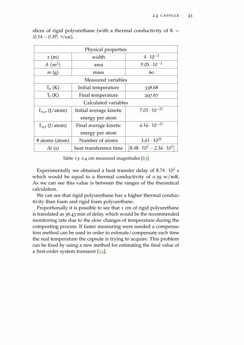
2.4 capsule 43
slices of rigid polyurethane (with a thermal conductivity of K =
[0.14− 0.39] w/mK).
Physical properties
x (m) width 4 · 10−3
A(m2)
area 9.05 · 10−3
m (g) mass 60
Measured variables
To (K) Initial temperature 338.68
Tf (K) Final temperature 297.67
Calculated variables
Ea,o (J/atom) Initial average kinetic 7.01 · 10−21
energy per atom
Ea,f (J/atom) Final average kinetic 6.16 · 10−21
energy per atom
# atoms (atom) Number of atoms 3.61 · 1025
∆t (s) heat transference time[8.48 · 102 − 2.36 · 103
]Table 13: 0.4 cm measured magnitudes [63]
Experimentally we obtained a heat transfer delay of 8.74 · 102 swhich would be equal to a thermal conductivity of 0.39 w/mK.As we can see this value is between the ranges of the theoreticalcalculation.
We can see that rigid polyurethane has a higher thermal conduc-tivity than foam and rigid foam polyurethane.
Proportionally it is possible to see that 1 cm of rigid polyurethaneis translated as 36.43 min of delay, which would be the recommendedmonitoring rate due to the slow changes of temperature during thecomposting process. If faster measuring were needed a compensa-tion method can be used in order to estimate/compensate each timethe real temperature the capsule is trying to acquire. This problemcan be fixed by using a new method for estimating the final value ofa first-order system transient [33].
44 temperature system
2.4.3 Method for reducing response time in sensor measurement
The previous section has stated the type of delay provoked by aplain model. However, we state that we are going to use a sphericcapsule. The heat transfer equation for a spherical model is [64]
1
r2∂
∂r
(r2∂T
∂r
)+
1
r2sin„∂
∂θ
(sinθ
∂T
∂θ
)+
1
r2sinθ∂2T
∂φ2+qG
k=1
α
∂T
∂t
(2.35)
As can be seen the equation has three space coordinates (r, θ , φ)and time (t) as variables. This implies a complex analysis that woulde presumably better analyzed through simulation. Nevertheles, thecase we propose is placing a plain 15 x 3 mm Pt 1000 sensor sep-arated 2 mm from the edge of a spheric capsule of radius 90 mm.If we calculate the volume of sphere section in front of the sensorwe obtain 85,32 mm3, whilst if it were a plain section it would be 90
mm3. This gives a volume error of 5.21 %. This volume error will notbe much relevant when concluding that for a plain section or for asphere section the delay provoked in the measure is a predominatingfirst order system.
Many sensor and instrumentation systems may have transientsthat extend their operation time, although they may sometimes giveinformation about a measured quantity[65]. As a result, many tran-sient analysis have been developed for this purpose[66]. When noinformation is contributed by the transient, it is desirable to reducethe time required to find the final value. Temperature systems are atypical example of systems in which transients are always present formeasurement purposes[67], for instance, sensor systems containedin enclosures. Therefore, when two bodies of different temperaturesare brought into contact, energy will flow spontaneously from oneto the other[68]. This flow takes a certain time to be completed be-fore the bodies reach a thermal equilibrium state. This effect maybe critical in certain situations. We may have a very slow systemin which a long time is required to receive the final value, or anautonomous system in which sample-taking is a critical factor forthe battery life. Most of these system transients, in temperature orsimilar applications, are modeled as first-order systems[69], andthe trend is often to use methods to optimally reduce the order ofsystems[70].
Solutions already exist for measuring time reduction, but theyusually involve complex calculations such as estimating the delaythrough complex operations[71]. Our objective now is to look for
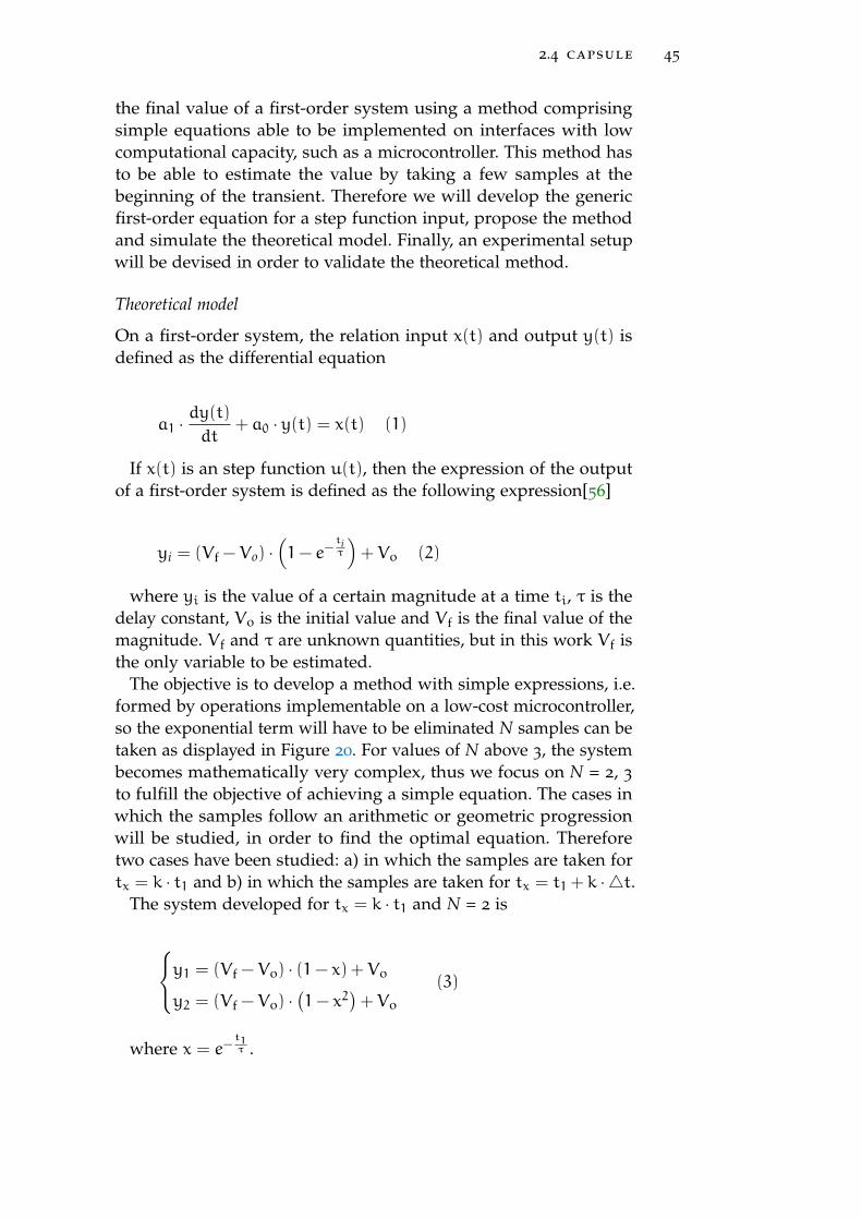
2.4 capsule 45
the final value of a first-order system using a method comprisingsimple equations able to be implemented on interfaces with lowcomputational capacity, such as a microcontroller. This method hasto be able to estimate the value by taking a few samples at thebeginning of the transient. Therefore we will develop the genericfirst-order equation for a step function input, propose the methodand simulate the theoretical model. Finally, an experimental setupwill be devised in order to validate the theoretical method.
Theoretical model
On a first-order system, the relation input x(t) and output y(t) isdefined as the differential equation
a1 ·dy(t)
dt+ a0 · y(t) = x(t) (1)
If x(t) is an step function u(t), then the expression of the outputof a first-order system is defined as the following expression[56]
yi = (V f − Vo) ·(1− e−
tiτ
)+ Vo (2)
where yi is the value of a certain magnitude at a time ti, τ is thedelay constant, Vo is the initial value and V f is the final value of themagnitude. V f and τ are unknown quantities, but in this work V f isthe only variable to be estimated.
The objective is to develop a method with simple expressions, i.e.formed by operations implementable on a low-cost microcontroller,so the exponential term will have to be eliminated N samples can betaken as displayed in Figure 20. For values of N above 3, the systembecomes mathematically very complex, thus we focus on N = 2, 3
to fulfill the objective of achieving a simple equation. The cases inwhich the samples follow an arithmetic or geometric progressionwill be studied, in order to find the optimal equation. Thereforetwo cases have been studied: a) in which the samples are taken fortx = k · t1 and b) in which the samples are taken for tx = t1 + k · 4t.
The system developed for tx = k · t1 and N = 2 is
y1 = (V f − Vo) · (1− x) + Vo
y2 = (V f − Vo) ·(1− x2
)+ Vo
(3)
where x = e−t1τ .
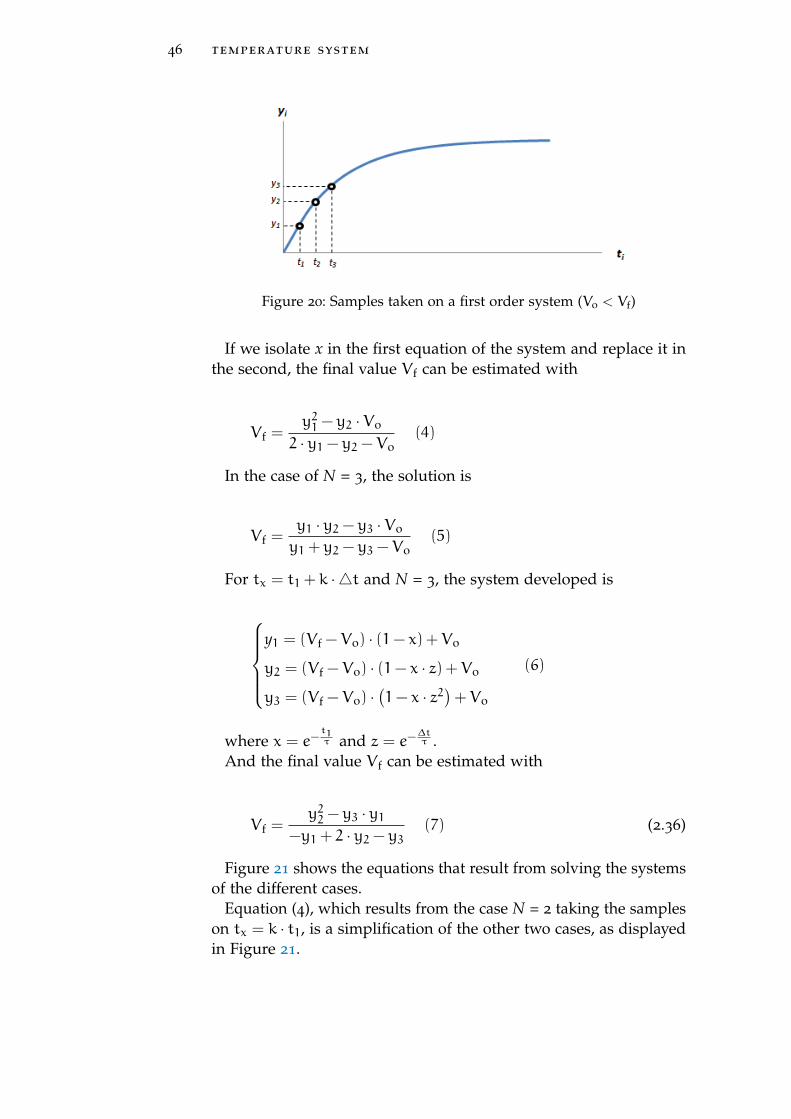
46 temperature system
Figure 20: Samples taken on a first order system (Vo < Vf)
If we isolate x in the first equation of the system and replace it inthe second, the final value V f can be estimated with
V f =y21 − y2 · Vo
2 · y1 − y2 − Vo(4)
In the case of N = 3, the solution is
V f =y1 · y2 − y3 · Vo
y1 + y2 − y3 − Vo(5)
For tx = t1 + k · 4t and N = 3, the system developed is
y1 = (V f − Vo) · (1− x) + Vo
y2 = (V f − Vo) · (1− x · z) + Vo
y3 = (V f − Vo) ·(1− x · z2
)+ Vo
(6)
where x = e−t1τ and z = e−
∆tτ .
And the final value V f can be estimated with
V f =y22 − y3 · y1
−y1 + 2 · y2 − y3(7) (2.36)
Figure 21 shows the equations that result from solving the systemsof the different cases.
Equation (4), which results from the case N = 2 taking the sampleson tx = k · t1, is a simplification of the other two cases, as displayedin Figure 21.
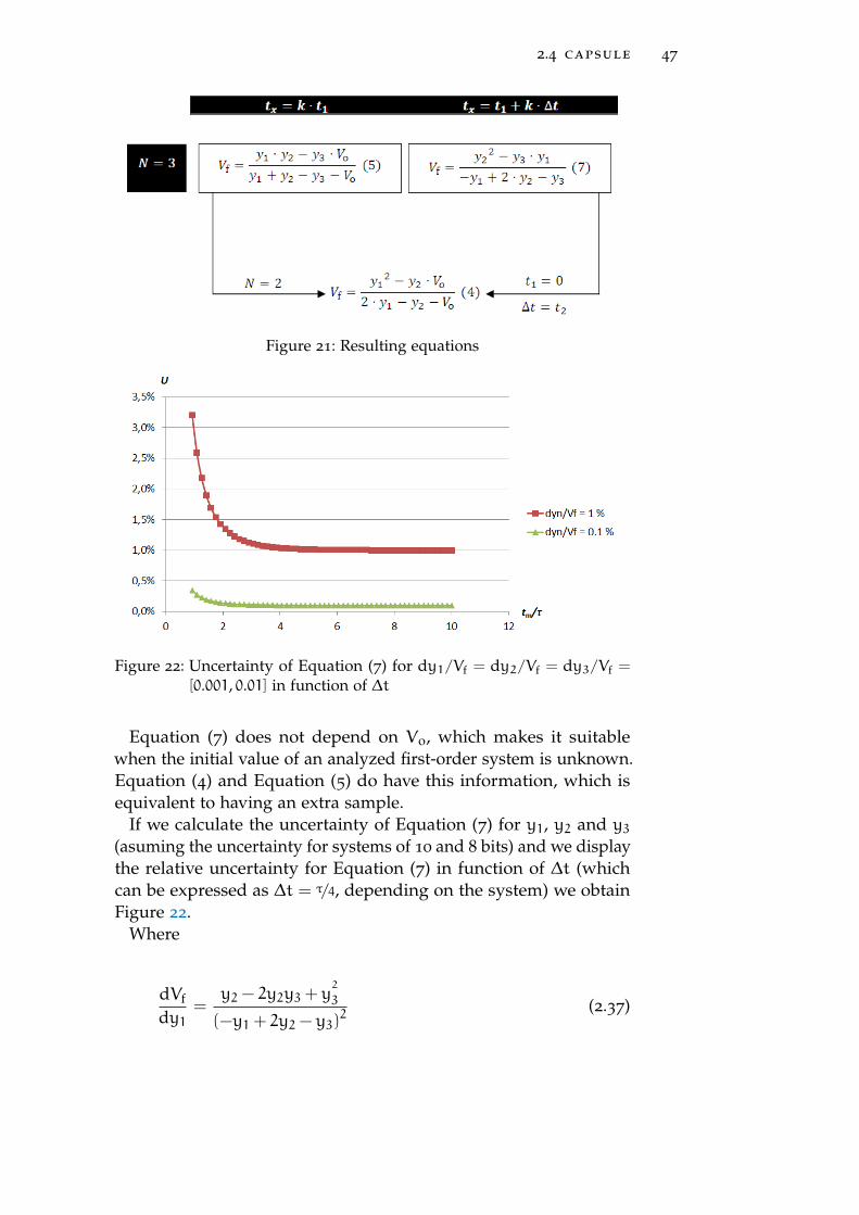
2.4 capsule 47
Figure 21: Resulting equations
Figure 22: Uncertainty of Equation (7) for dy1/Vf = dy2/Vf = dy3/Vf =[0.001, 0.01] in function of ∆t
Equation (7) does not depend on Vo, which makes it suitablewhen the initial value of an analyzed first-order system is unknown.Equation (4) and Equation (5) do have this information, which isequivalent to having an extra sample.
If we calculate the uncertainty of Equation (7) for y1, y2 and y3(asuming the uncertainty for systems of 10 and 8 bits) and we displaythe relative uncertainty for Equation (7) in function of ∆t (whichcan be expressed as ∆t = τ/4, depending on the system) we obtainFigure 22.
Where
dVf
dy1=
y2 − 2y2y3 + y2
3
(−y1 + 2y2 − y3)2
(2.37)
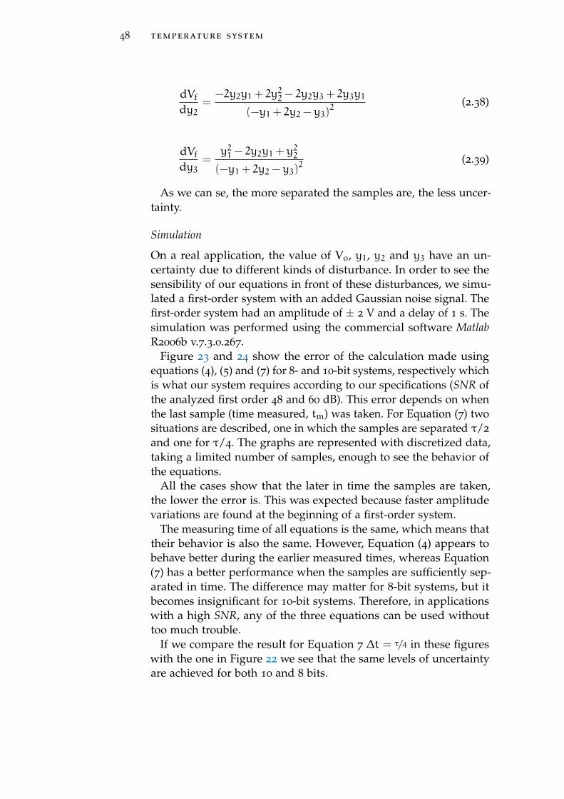
48 temperature system
dVf
dy2=
−2y2y1 + 2y22 − 2y2y3 + 2y3y1
(−y1 + 2y2 − y3)2
(2.38)
dVf
dy3=
y21 − 2y2y1 + y22
(−y1 + 2y2 − y3)2
(2.39)
As we can se, the more separated the samples are, the less uncer-tainty.
Simulation
On a real application, the value of Vo, y1, y2 and y3 have an un-certainty due to different kinds of disturbance. In order to see thesensibility of our equations in front of these disturbances, we simu-lated a first-order system with an added Gaussian noise signal. Thefirst-order system had an amplitude of ± 2 V and a delay of 1 s. Thesimulation was performed using the commercial software MatlabR2006b v.7.3.0.267.
Figure 23 and 24 show the error of the calculation made usingequations (4), (5) and (7) for 8- and 10-bit systems, respectively whichis what our system requires according to our specifications (SNR ofthe analyzed first order 48 and 60 dB). This error depends on whenthe last sample (time measured, tm) was taken. For Equation (7) twosituations are described, one in which the samples are separated τ/2
and one for τ/4. The graphs are represented with discretized data,taking a limited number of samples, enough to see the behavior ofthe equations.
All the cases show that the later in time the samples are taken,the lower the error is. This was expected because faster amplitudevariations are found at the beginning of a first-order system.
The measuring time of all equations is the same, which means thattheir behavior is also the same. However, Equation (4) appears tobehave better during the earlier measured times, whereas Equation(7) has a better performance when the samples are sufficiently sep-arated in time. The difference may matter for 8-bit systems, but itbecomes insignificant for 10-bit systems. Therefore, in applicationswith a high SNR, any of the three equations can be used withouttoo much trouble.
If we compare the result for Equation 7 ∆t = τ/4 in these figureswith the one in Figure 22 we see that the same levels of uncertaintyare achieved for both 10 and 8 bits.
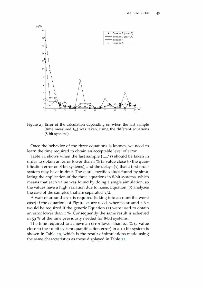
2.4 capsule 49
Figure 23: Error of the calculation depending on when the last sample(time measured tm) was taken, using the different equations(8-bit systems)
Once the behavior of the three equations is known, we need tolearn the time required to obtain an acceptable level of error.
Table 14 shows when the last sample (tm/τ) should be taken inorder to obtain an error lower than 1 % (a value close to the quan-tification error on 8-bit systems), and the delays (τ) that a first-ordersystem may have in time. These are specific values found by simu-lating the application of the three equations in 8-bit systems, whichmeans that each value was found by doing a single simulation, sothe values have a high variation due to noise. Equation (7) analyzesthe case of the samples that are separated τ/2.
A wait of around 2.7·τ is required (taking into account the worstcase) if the equations of Figure 21 are used, whereas around 4.6·τwould be required if the generic Equation (2) were used to obtainan error lower than 1 %. Consequently the same result is achievedin 59 % of the time previously needed for 8-bit systems.
The time required to achieve an error lower than 0.1 % (a valueclose to the 10-bit system quantification error) in a 10-bit system isshown in Table 15, which is the result of simulations made usingthe same characteristics as those displayed in Table 21.
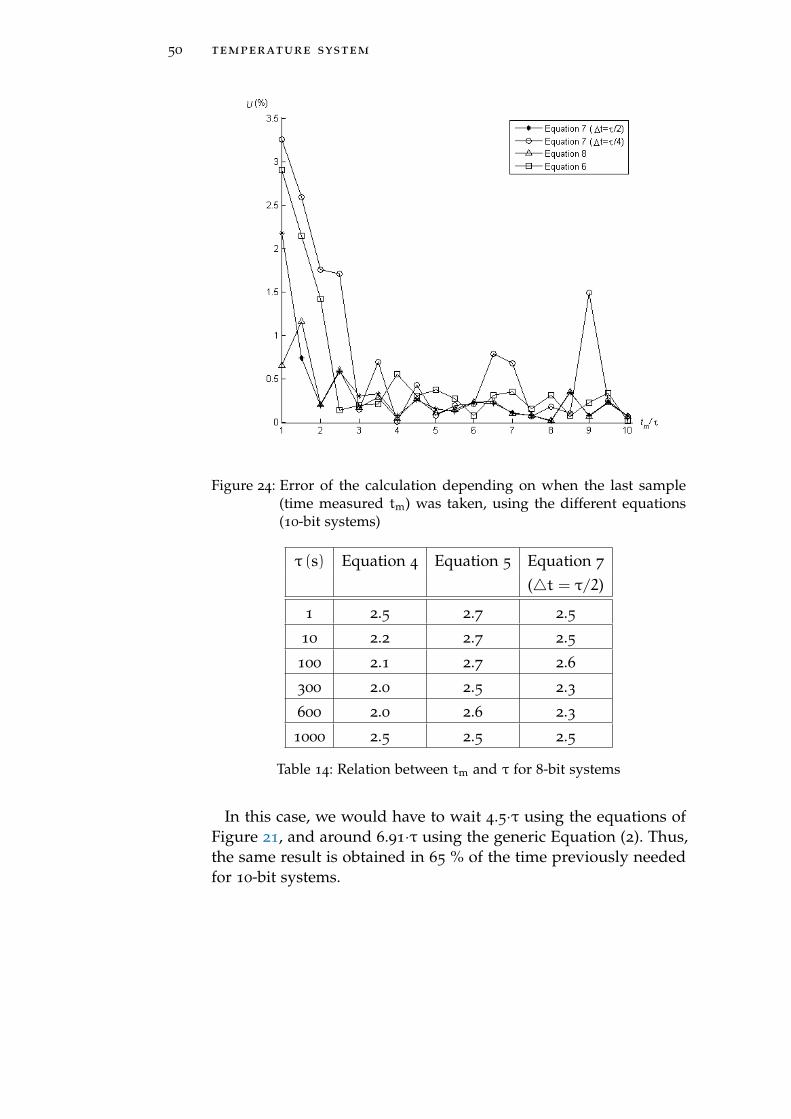
50 temperature system
Figure 24: Error of the calculation depending on when the last sample(time measured tm) was taken, using the different equations(10-bit systems)
τ (s) Equation 4 Equation 5 Equation 7
(4t = τ/2)
1 2.5 2.7 2.5
10 2.2 2.7 2.5
100 2.1 2.7 2.6
300 2.0 2.5 2.3
600 2.0 2.6 2.3
1000 2.5 2.5 2.5
Table 14: Relation between tm and τ for 8-bit systems
In this case, we would have to wait 4.5·τ using the equations ofFigure 21, and around 6.91·τ using the generic Equation (2). Thus,the same result is obtained in 65 % of the time previously neededfor 10-bit systems.
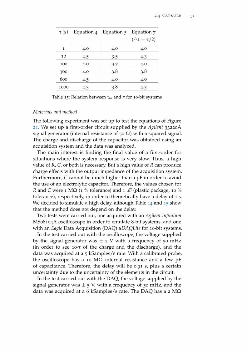
2.4 capsule 51
τ (s) Equation 4 Equation 5 Equation 7
(4t = τ/2)
1 4.0 4.0 4.0
10 4.5 3.5 4.3
100 4.0 3.7 4.0
300 4.0 3.8 3.8
600 4.5 4.0 4.0
1000 4.3 3.8 4.3
Table 15: Relation between tm and τ for 10-bit systems
Materials and method
The following experiment was set up to test the equations of Figure21. We set up a first-order circuit supplied by the Agilent 33220Asignal generator (internal resistance of 50 Ω) with a squared signal.The charge and discharge of the capacitor was obtained using anacquisition system and the data was analyzed.
The main interest is finding the final value of a first-order forsituations where the system response is very slow. Thus, a highvalue of R, C, or both is necessary. But a high value of R can producecharge effects with the output impedance of the acquisition system.Furthermore, C cannot be much higher than 1 μF in order to avoidthe use of an electrolytic capacitor. Therefore, the values chosen forR and C were 1 MΩ (1 % tolerance) and 1 μF (plastic package, 10 %tolerance), respectively, in order to theoretically have a delay of 1 s.We decided to simulate a high delay, although Table 14 and 15 showthat the method does not depend on the delay.
Two tests were carried out, one acquired with an Agilent InfiniiumMS08104A oscilloscope in order to emulate 8-bit systems, and onewith an Eagle Data Acquisition (DAQ) uDAQLite for 10-bit systems.
In the test carried out with the oscilloscope, the voltage suppliedby the signal generator was ± 2 V with a frequency of 50 mHz(in order to see 10·τ of the charge and the discharge), and thedata was acquired at a 5 kSamples/s rate. With a calibrated probe,the oscilloscope has a 10 MΩ internal resistance and a few pFof capacitance. Therefore, the delay will be 0.91 s, plus a certainuncertainty due to the uncertainty of the elements in the circuit.
In the test carried out with the DAQ, the voltage supplied by thesignal generator was ± 5 V, with a frequency of 50 mHz, and thedata was acquired at a 6 kSamples/s rate. The DAQ has a 2 MΩ
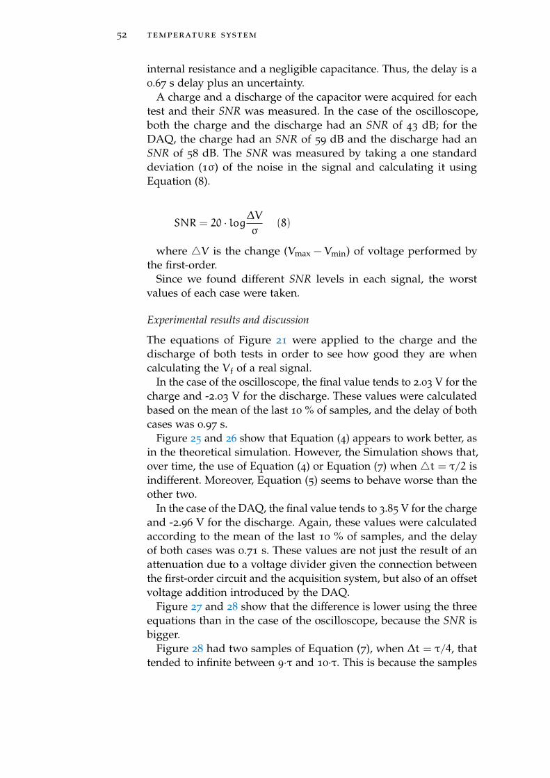
52 temperature system
internal resistance and a negligible capacitance. Thus, the delay is a0.67 s delay plus an uncertainty.
A charge and a discharge of the capacitor were acquired for eachtest and their SNR was measured. In the case of the oscilloscope,both the charge and the discharge had an SNR of 43 dB; for theDAQ, the charge had an SNR of 59 dB and the discharge had anSNR of 58 dB. The SNR was measured by taking a one standarddeviation (1σ) of the noise in the signal and calculating it usingEquation (8).
SNR = 20 · log∆Vσ
(8)
where 4V is the change (Vmax − Vmin) of voltage performed bythe first-order.
Since we found different SNR levels in each signal, the worstvalues of each case were taken.
Experimental results and discussion
The equations of Figure 21 were applied to the charge and thedischarge of both tests in order to see how good they are whencalculating the V f of a real signal.
In the case of the oscilloscope, the final value tends to 2.03 V for thecharge and -2.03 V for the discharge. These values were calculatedbased on the mean of the last 10 % of samples, and the delay of bothcases was 0.97 s.
Figure 25 and 26 show that Equation (4) appears to work better, asin the theoretical simulation. However, the Simulation shows that,over time, the use of Equation (4) or Equation (7) when 4t = τ/2 isindifferent. Moreover, Equation (5) seems to behave worse than theother two.
In the case of the DAQ, the final value tends to 3.85 V for the chargeand -2.96 V for the discharge. Again, these values were calculatedaccording to the mean of the last 10 % of samples, and the delayof both cases was 0.71 s. These values are not just the result of anattenuation due to a voltage divider given the connection betweenthe first-order circuit and the acquisition system, but also of an offsetvoltage addition introduced by the DAQ.
Figure 27 and 28 show that the difference is lower using the threeequations than in the case of the oscilloscope, because the SNR isbigger.
Figure 28 had two samples of Equation (7), when ∆t = τ/4, thattended to infinite between 9·τ and 10·τ. This is because the samples
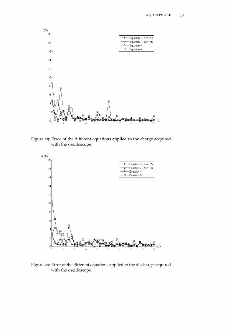
2.4 capsule 53
Figure 25: Error of the different equations applied to the charge acquiredwith the oscilloscope
Figure 26: Error of the different equations applied to the discharge acquiredwith the oscilloscope
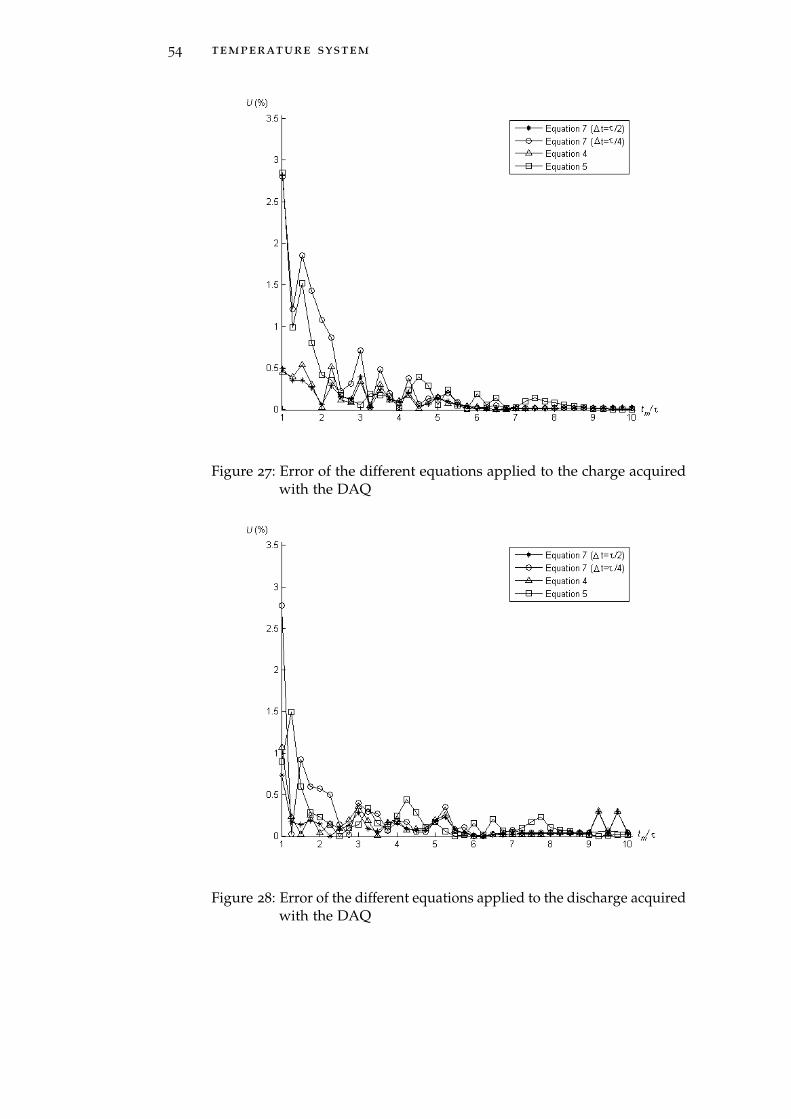
54 temperature system
Figure 27: Error of the different equations applied to the charge acquiredwith the DAQ
Figure 28: Error of the different equations applied to the discharge acquiredwith the DAQ
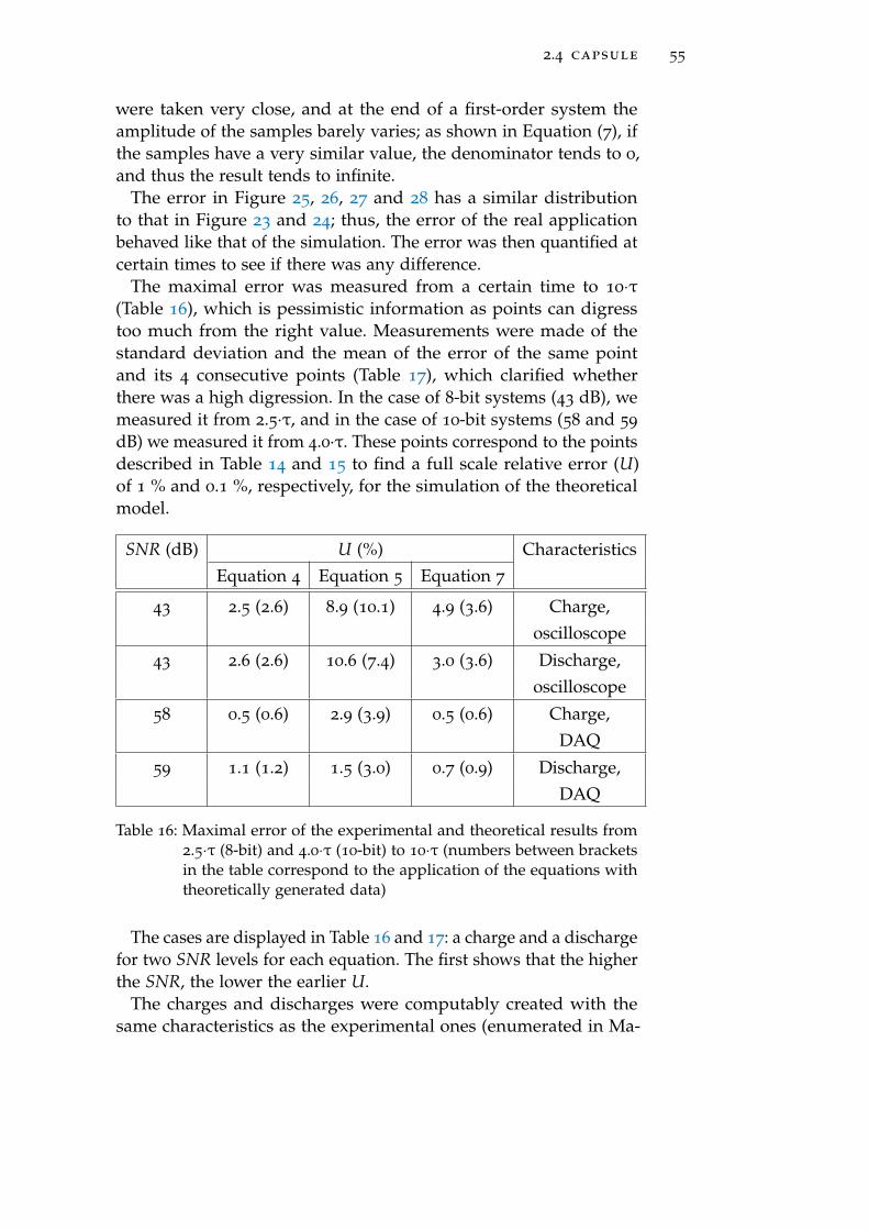
2.4 capsule 55
were taken very close, and at the end of a first-order system theamplitude of the samples barely varies; as shown in Equation (7), ifthe samples have a very similar value, the denominator tends to 0,and thus the result tends to infinite.
The error in Figure 25, 26, 27 and 28 has a similar distributionto that in Figure 23 and 24; thus, the error of the real applicationbehaved like that of the simulation. The error was then quantified atcertain times to see if there was any difference.
The maximal error was measured from a certain time to 10·τ(Table 16), which is pessimistic information as points can digresstoo much from the right value. Measurements were made of thestandard deviation and the mean of the error of the same pointand its 4 consecutive points (Table 17), which clarified whetherthere was a high digression. In the case of 8-bit systems (43 dB), wemeasured it from 2.5·τ, and in the case of 10-bit systems (58 and 59
dB) we measured it from 4.0·τ. These points correspond to the pointsdescribed in Table 14 and 15 to find a full scale relative error (U)of 1 % and 0.1 %, respectively, for the simulation of the theoreticalmodel.
SNR (dB) U (%) CharacteristicsEquation 4 Equation 5 Equation 7
43 2.5 (2.6) 8.9 (10.1) 4.9 (3.6) Charge,oscilloscope
43 2.6 (2.6) 10.6 (7.4) 3.0 (3.6) Discharge,oscilloscope
58 0.5 (0.6) 2.9 (3.9) 0.5 (0.6) Charge,DAQ
59 1.1 (1.2) 1.5 (3.0) 0.7 (0.9) Discharge,DAQ
Table 16: Maximal error of the experimental and theoretical results from2.5·τ (8-bit) and 4.0·τ (10-bit) to 10·τ (numbers between bracketsin the table correspond to the application of the equations withtheoretically generated data)
The cases are displayed in Table 16 and 17: a charge and a dischargefor two SNR levels for each equation. The first shows that the higherthe SNR, the lower the earlier U.
The charges and discharges were computably created with thesame characteristics as the experimental ones (enumerated in Ma-
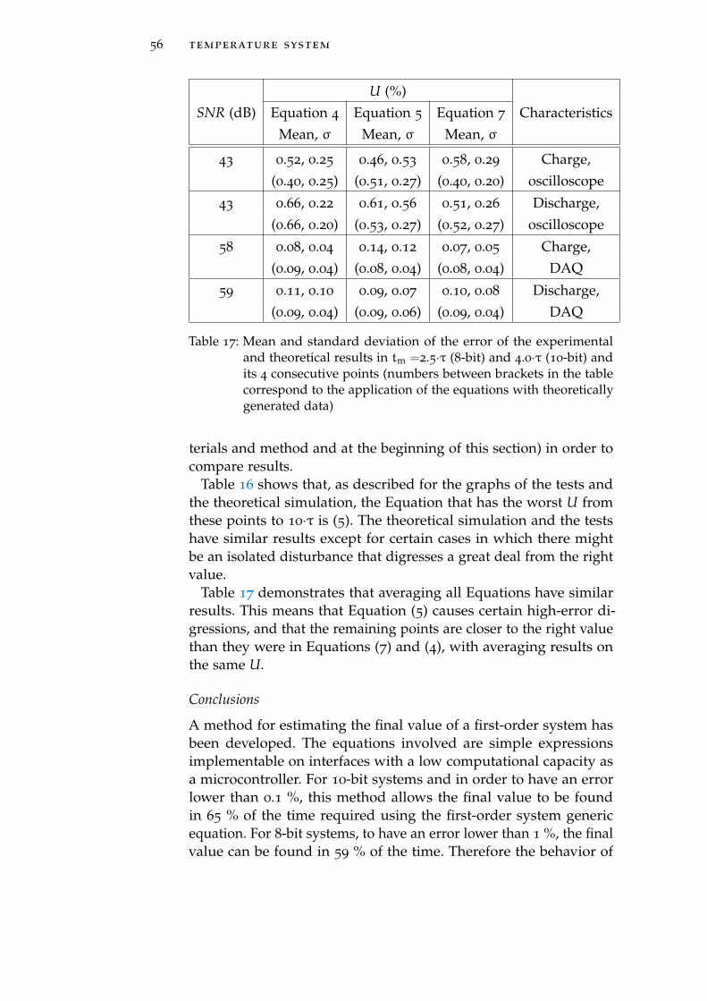
56 temperature system
U (%)SNR (dB) Equation 4 Equation 5 Equation 7 Characteristics
Mean, σ Mean, σ Mean, σ
43 0.52, 0.25 0.46, 0.53 0.58, 0.29 Charge,(0.40, 0.25) (0.51, 0.27) (0.40, 0.20) oscilloscope
43 0.66, 0.22 0.61, 0.56 0.51, 0.26 Discharge,(0.66, 0.20) (0.53, 0.27) (0.52, 0.27) oscilloscope
58 0.08, 0.04 0.14, 0.12 0.07, 0.05 Charge,(0.09, 0.04) (0.08, 0.04) (0.08, 0.04) DAQ
59 0.11, 0.10 0.09, 0.07 0.10, 0.08 Discharge,(0.09, 0.04) (0.09, 0.06) (0.09, 0.04) DAQ
Table 17: Mean and standard deviation of the error of the experimentaland theoretical results in tm =2.5·τ (8-bit) and 4.0·τ (10-bit) andits 4 consecutive points (numbers between brackets in the tablecorrespond to the application of the equations with theoreticallygenerated data)
terials and method and at the beginning of this section) in order tocompare results.
Table 16 shows that, as described for the graphs of the tests andthe theoretical simulation, the Equation that has the worst U fromthese points to 10·τ is (5). The theoretical simulation and the testshave similar results except for certain cases in which there mightbe an isolated disturbance that digresses a great deal from the rightvalue.
Table 17 demonstrates that averaging all Equations have similarresults. This means that Equation (5) causes certain high-error di-gressions, and that the remaining points are closer to the right valuethan they were in Equations (7) and (4), with averaging results onthe same U.
Conclusions
A method for estimating the final value of a first-order system hasbeen developed. The equations involved are simple expressionsimplementable on interfaces with a low computational capacity asa microcontroller. For 10-bit systems and in order to have an errorlower than 0.1 %, this method allows the final value to be foundin 65 % of the time required using the first-order system genericequation. For 8-bit systems, to have an error lower than 1 %, the finalvalue can be found in 59 % of the time. Therefore the behavior of
2.5 conclusions 57
the error in the calculation is lower earlier, and if we wish to reducethe possibility of having negative digressions on the error we canrealize the mean of calculations taking the samples at consecutivemoments.
The model can be used in our autonomous system to save process-ing time and thus decrease its overall consumption with a negligibleerror introduction.
2.5 conclusions
We have designed a temperature system that autonomously mea-sures temperature of compost from the inside of a capsule. Thefollowing conclusions have been extracted from the development:
1. We have compared two different conditioning methods: classicconditioning and a direct interface sensor-to-microcontroller.We found that the main consumer of the classic consumptionis the excitation stage and that depending on that varyingthe resistances the consumption/resolution trade-off can beoptimized. The direct interface method has proved to consumemuch less than the classic conditioning at the cost of someresolution. Still the resolution provided by the direct interfacemethod is more than enoguh for most of temperature sensingapplications.
2. We have studied different materials for the protection of thecircuit and found that depending on the material the delay onthe sensing of temeprature varies.
3. To counteract the delay in the temperature measuring we havedeveloped an algorithm to estimate the final value of the de-layed measure of temperature. In other words, while the out-side temperature is being acquired by the whole body of thecircuit protective material at the rate of a first order, our algo-rithm can estimate what the temperature is by taking someinitial samples reducing the measuring time to 60 % of what itwould take otherwise.
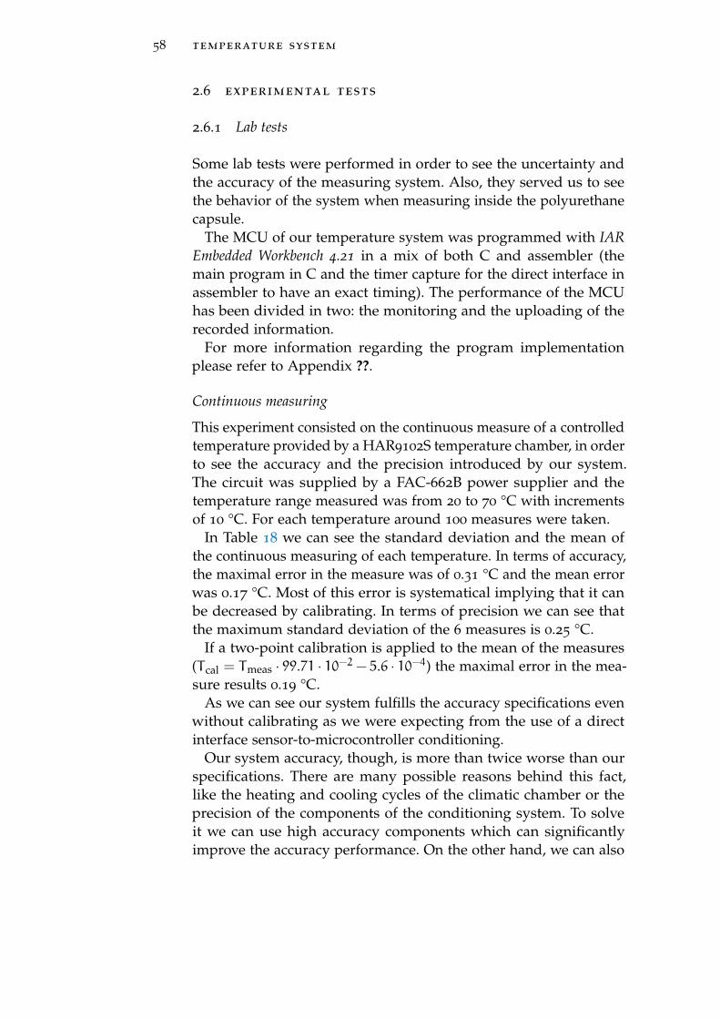
58 temperature system
2.6 experimental tests
2.6.1 Lab tests
Some lab tests were performed in order to see the uncertainty andthe accuracy of the measuring system. Also, they served us to seethe behavior of the system when measuring inside the polyurethanecapsule.
The MCU of our temperature system was programmed with IAREmbedded Workbench 4.21 in a mix of both C and assembler (themain program in C and the timer capture for the direct interface inassembler to have an exact timing). The performance of the MCUhas been divided in two: the monitoring and the uploading of therecorded information.
For more information regarding the program implementationplease refer to Appendix ??.
Continuous measuring
This experiment consisted on the continuous measure of a controlledtemperature provided by a HAR9102S temperature chamber, in orderto see the accuracy and the precision introduced by our system.The circuit was supplied by a FAC-662B power supplier and thetemperature range measured was from 20 to 70 °C with incrementsof 10 °C. For each temperature around 100 measures were taken.
In Table 18 we can see the standard deviation and the mean ofthe continuous measuring of each temperature. In terms of accuracy,the maximal error in the measure was of 0.31 °C and the mean errorwas 0.17 °C. Most of this error is systematical implying that it canbe decreased by calibrating. In terms of precision we can see thatthe maximum standard deviation of the 6 measures is 0.25 °C.
If a two-point calibration is applied to the mean of the measures(T cal = Tmeas · 99.71 · 10−2 − 5.6 · 10−4) the maximal error in the mea-sure results 0.19 °C.
As we can see our system fulfills the accuracy specifications evenwithout calibrating as we were expecting from the use of a directinterface sensor-to-microcontroller conditioning.
Our system accuracy, though, is more than twice worse than ourspecifications. There are many possible reasons behind this fact,like the heating and cooling cycles of the climatic chamber or theprecision of the components of the conditioning system. To solveit we can use high accuracy components which can significantlyimprove the accuracy performance. On the other hand, we can also
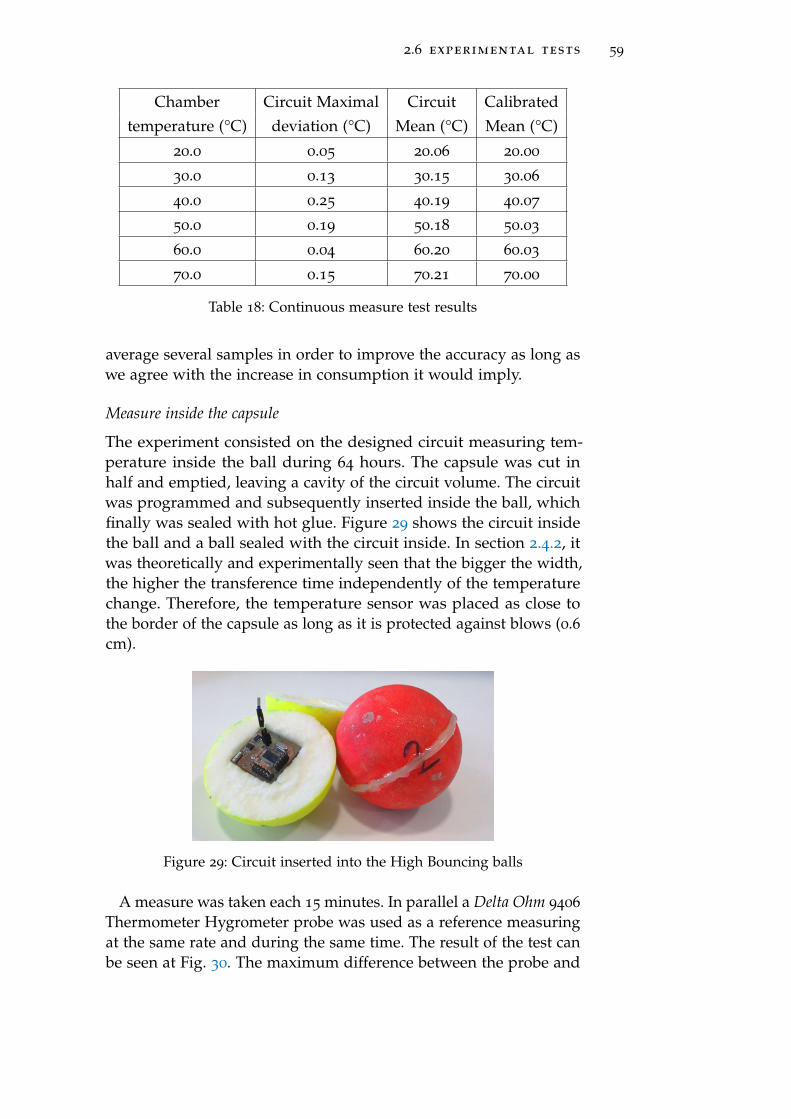
2.6 experimental tests 59
Chamber Circuit Maximal Circuit Calibratedtemperature (°C) deviation (°C) Mean (°C) Mean (°C)
20.0 0.05 20.06 20.00
30.0 0.13 30.15 30.06
40.0 0.25 40.19 40.07
50.0 0.19 50.18 50.03
60.0 0.04 60.20 60.03
70.0 0.15 70.21 70.00
Table 18: Continuous measure test results
average several samples in order to improve the accuracy as long aswe agree with the increase in consumption it would imply.
Measure inside the capsule
The experiment consisted on the designed circuit measuring tem-perature inside the ball during 64 hours. The capsule was cut inhalf and emptied, leaving a cavity of the circuit volume. The circuitwas programmed and subsequently inserted inside the ball, whichfinally was sealed with hot glue. Figure 29 shows the circuit insidethe ball and a ball sealed with the circuit inside. In section 2.4.2, itwas theoretically and experimentally seen that the bigger the width,the higher the transference time independently of the temperaturechange. Therefore, the temperature sensor was placed as close tothe border of the capsule as long as it is protected against blows (0.6cm).
Figure 29: Circuit inserted into the High Bouncing balls
A measure was taken each 15 minutes. In parallel a Delta Ohm 9406
Thermometer Hygrometer probe was used as a reference measuringat the same rate and during the same time. The result of the test canbe seen at Fig. 30. The maximum difference between the probe and
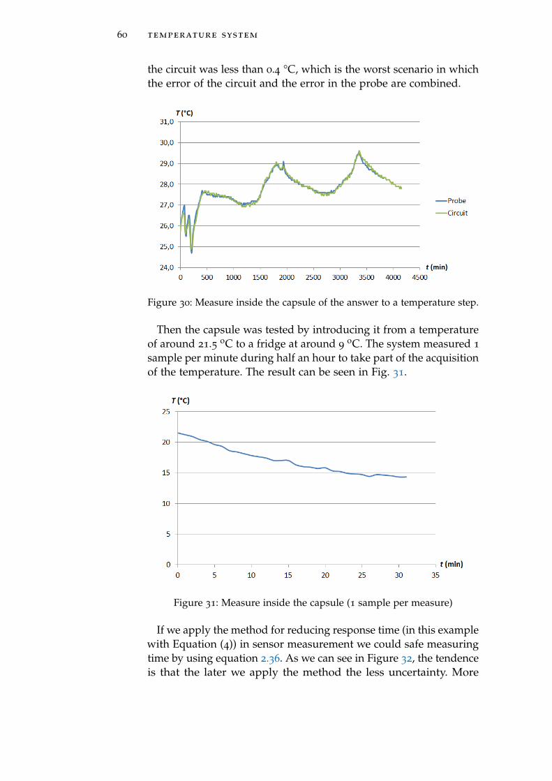
60 temperature system
the circuit was less than 0.4 °C, which is the worst scenario in whichthe error of the circuit and the error in the probe are combined.
Figure 30: Measure inside the capsule of the answer to a temperature step.
Then the capsule was tested by introducing it from a temperatureof around 21.5 oC to a fridge at around 9
oC. The system measured 1
sample per minute during half an hour to take part of the acquisitionof the temperature. The result can be seen in Fig. 31.
Figure 31: Measure inside the capsule (1 sample per measure)
If we apply the method for reducing response time (in this examplewith Equation (4)) in sensor measurement we could safe measuringtime by using equation 2.36. As we can see in Figure 32, the tendenceis that the later we apply the method the less uncertainty. More
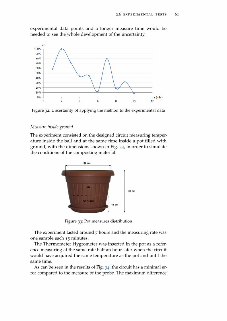
2.6 experimental tests 61
experimental data points and a longer measure time would beneeded to see the whole development of the uncertainty.
Figure 32: Uncertainty of applying the method to the experimental data
Measure inside ground
The experiment consisted on the designed circuit measuring temper-ature inside the ball and at the same time inside a pot filled withground, with the dimensions shown in Fig. 33, in order to simulatethe conditions of the composting material.
Figure 33: Pot measures distribution
The experiment lasted around 7 hours and the measuring rate wasone sample each 15 minutes.
The Thermometer Hygrometer was inserted in the pot as a refer-ence measuring at the same rate half an hour later when the circuitwould have acquired the same temperature as the pot and until thesame time.
As can be seen in the results of Fig. 34, the circuit has a minimal er-ror compared to the measure of the probe. The maximum difference
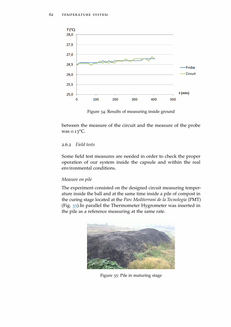
62 temperature system
Figure 34: Results of measuring inside ground
between the measure of the circuit and the measure of the probewas 0.13
oC.
2.6.2 Field tests
Some field test measures are needed in order to check the properoperation of our system inside the capsule and within the realenvironmental conditions.
Measure on pile
The experiment consisted on the designed circuit measuring temper-ature inside the ball and at the same time inside a pile of compost inthe curing stage located at the Parc Mediterrani de la Tecnologia (PMT)(Fig. 35).In parallel the Thermometer Hygrometer was inserted inthe pile as a reference measuring at the same rate.
Figure 35: Pile in maturing stage
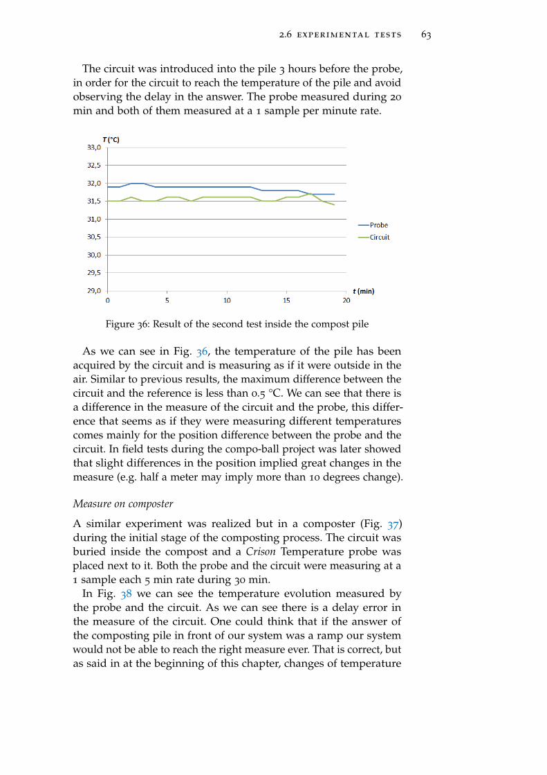
2.6 experimental tests 63
The circuit was introduced into the pile 3 hours before the probe,in order for the circuit to reach the temperature of the pile and avoidobserving the delay in the answer. The probe measured during 20
min and both of them measured at a 1 sample per minute rate.
Figure 36: Result of the second test inside the compost pile
As we can see in Fig. 36, the temperature of the pile has beenacquired by the circuit and is measuring as if it were outside in theair. Similar to previous results, the maximum difference between thecircuit and the reference is less than 0.5 °C. We can see that there isa difference in the measure of the circuit and the probe, this differ-ence that seems as if they were measuring different temperaturescomes mainly for the position difference between the probe and thecircuit. In field tests during the compo-ball project was later showedthat slight differences in the position implied great changes in themeasure (e.g. half a meter may imply more than 10 degrees change).
Measure on composter
A similar experiment was realized but in a composter (Fig. 37)during the initial stage of the composting process. The circuit wasburied inside the compost and a Crison Temperature probe wasplaced next to it. Both the probe and the circuit were measuring at a1 sample each 5 min rate during 30 min.
In Fig. 38 we can see the temperature evolution measured bythe probe and the circuit. As we can see there is a delay error inthe measure of the circuit. One could think that if the answer ofthe composting pile in front of our system was a ramp our systemwould not be able to reach the right measure ever. That is correct, butas said in at the beginning of this chapter, changes of temperature
64 temperature system
Figure 37: Composter
during the composting process are really slow, and hence our systemwould be able to follow these changes with a smaller error. In thiscase, the change of temperature in 30 minutes is of 0.8oC and themaximum error between probe and circuit is of 0.3oC.
Figure 38: Test inside the composter
Also we can see that the maximum delay in the measure is of 7
minutes. The sensor was placed 3 mm inside the ball, and the ballwas a foam polyurethane ball, around 100 g and a 12 cm diameter.Theoretically, with this data the delay suffered by a measure shouldbe of 8.62 min. The reason why our measure is better is because themodel is not completely uniform and the sensor is not between twoequal masses and volumes, the delay decreases since its nearer fromthe heat focus due to the heat-transfer principles.
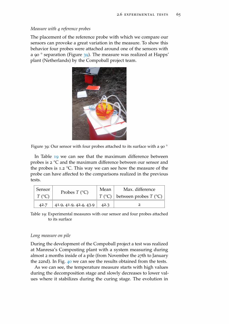
2.6 experimental tests 65
Measure with 4 reference probes
The placement of the reference probe with which we compare oursensors can provoke a great variation in the measure. To show thisbehavior four probes were attached around one of the sensors witha 90 ° separation (Figure 39). The measure was realized at Happs’plant (Netherlands) by the Compoball project team.
Figure 39: Our sensor with four probes attached to its surface with a 90 °
In Table 19 we can see that the maximum difference betweenprobes is 2 °C and the maximum difference between our sensor andthe probes is 1.2 °C. This way we can see how the measure of theprobe can have affected to the comparisons realized in the previoustests.
SensorProbes T (°C)
Mean Max. differenceT (°C) T (°C) between probes T (°C)
42.7 41.9, 41.9, 42.4, 43.9 42.3 2
Table 19: Experimental measures with our sensor and four probes attachedto its surface
Long measure on pile
During the development of the Compoball project a test was realizedat Manresa’s Composting plant with a system measuring duringalmost 2 months inside of a pile (from November the 27th to Januarythe 22nd). In Fig. 40 we can see the results obtained from the tests.
As we can see, the temperature measure starts with high valuesduring the decomposition stage and slowly decreases to lower val-ues where it stabilizes during the curing stage. The evolution in
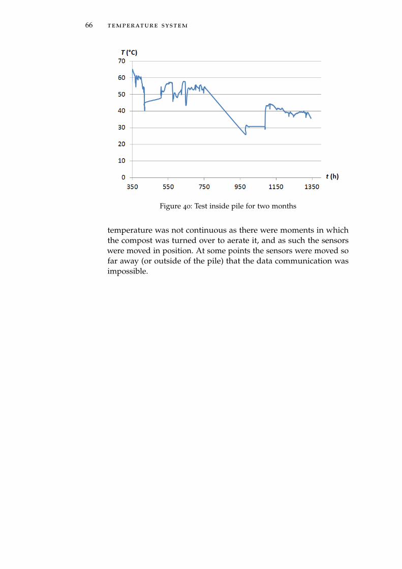
66 temperature system
Figure 40: Test inside pile for two months
temperature was not continuous as there were moments in whichthe compost was turned over to aerate it, and as such the sensorswere moved in position. At some points the sensors were moved sofar away (or outside of the pile) that the data communication wasimpossible.
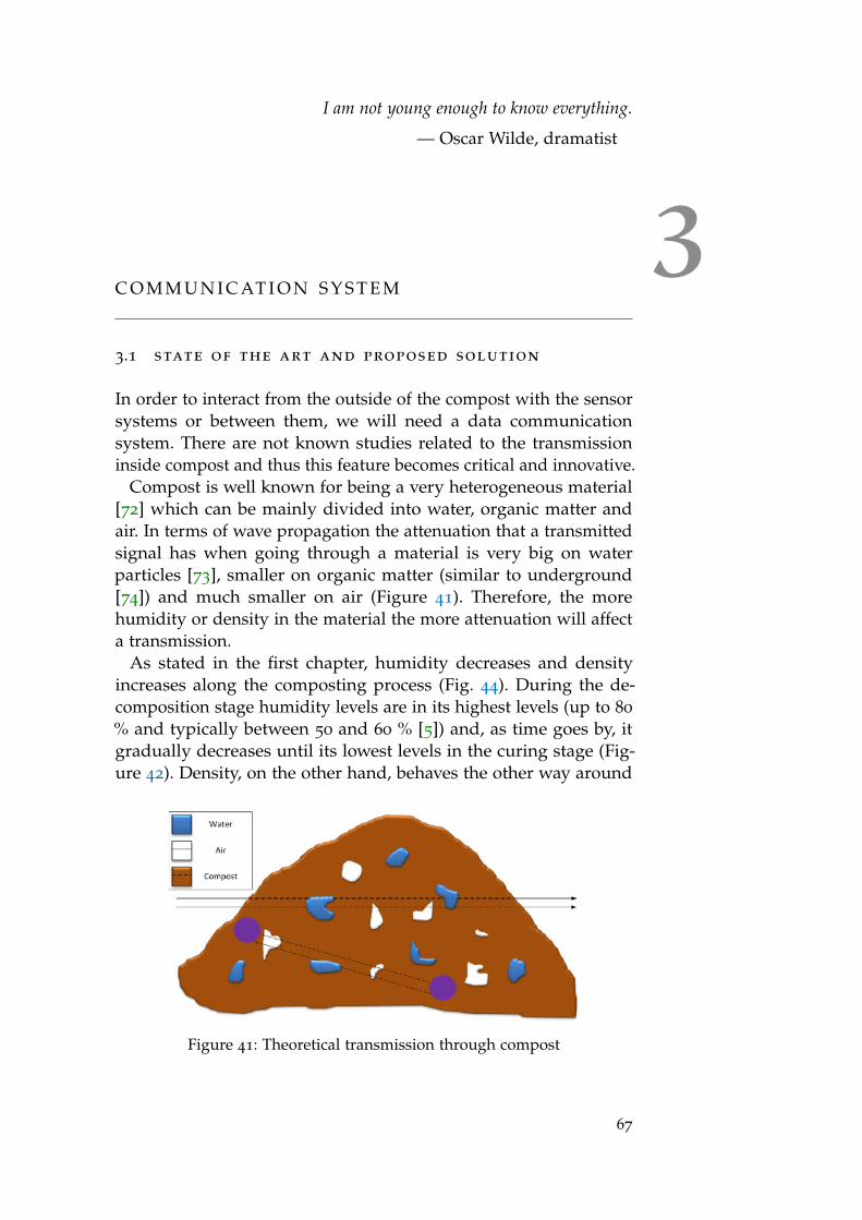
I am not young enough to know everything.
— Oscar Wilde, dramatist
3C O M M U N I C AT I O N S Y S T E M
3.1 state of the art and proposed solution
In order to interact from the outside of the compost with the sensorsystems or between them, we will need a data communicationsystem. There are not known studies related to the transmissioninside compost and thus this feature becomes critical and innovative.
Compost is well known for being a very heterogeneous material[72] which can be mainly divided into water, organic matter andair. In terms of wave propagation the attenuation that a transmittedsignal has when going through a material is very big on waterparticles [73], smaller on organic matter (similar to underground[74]) and much smaller on air (Figure 41). Therefore, the morehumidity or density in the material the more attenuation will affecta transmission.
As stated in the first chapter, humidity decreases and densityincreases along the composting process (Fig. 44). During the de-composition stage humidity levels are in its highest levels (up to 80
% and typically between 50 and 60 % [5]) and, as time goes by, itgradually decreases until its lowest levels in the curing stage (Fig-ure 42). Density, on the other hand, behaves the other way around
Figure 41: Theoretical transmission through compost
67
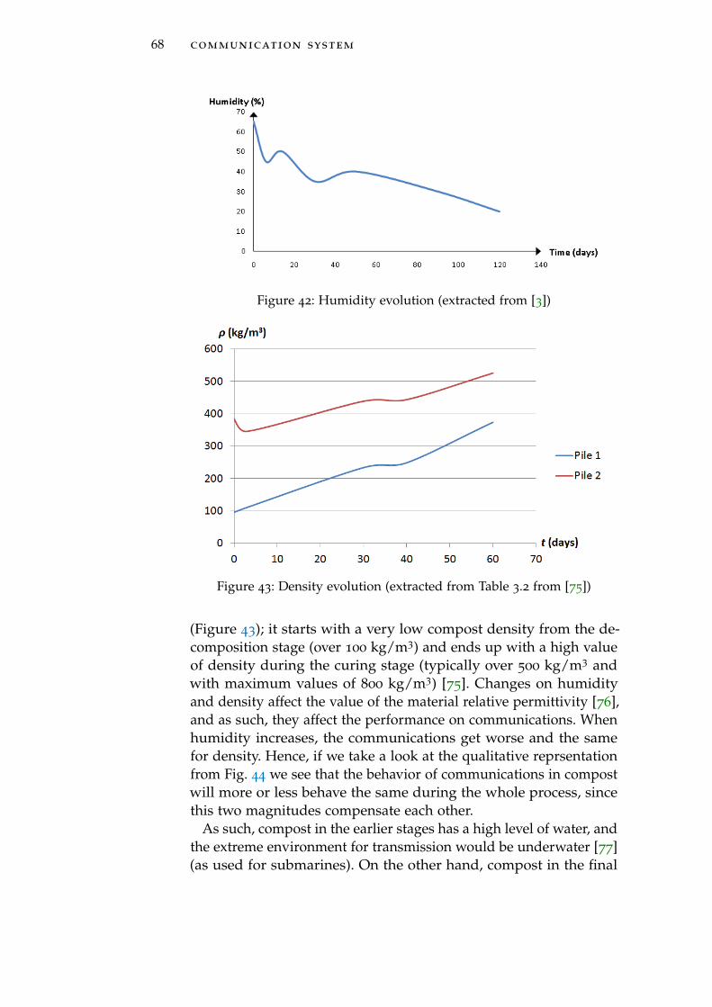
68 communication system
Figure 42: Humidity evolution (extracted from [3])
Figure 43: Density evolution (extracted from Table 3.2 from [75])
(Figure 43); it starts with a very low compost density from the de-composition stage (over 100 kg/m3) and ends up with a high valueof density during the curing stage (typically over 500 kg/m3 andwith maximum values of 800 kg/m3) [75]. Changes on humidityand density affect the value of the material relative permittivity [76],and as such, they affect the performance on communications. Whenhumidity increases, the communications get worse and the samefor density. Hence, if we take a look at the qualitative reprsentationfrom Fig. 44 we see that the behavior of communications in compostwill more or less behave the same during the whole process, sincethis two magnitudes compensate each other.
As such, compost in the earlier stages has a high level of water, andthe extreme environment for transmission would be underwater [77](as used for submarines). On the other hand, compost in the final
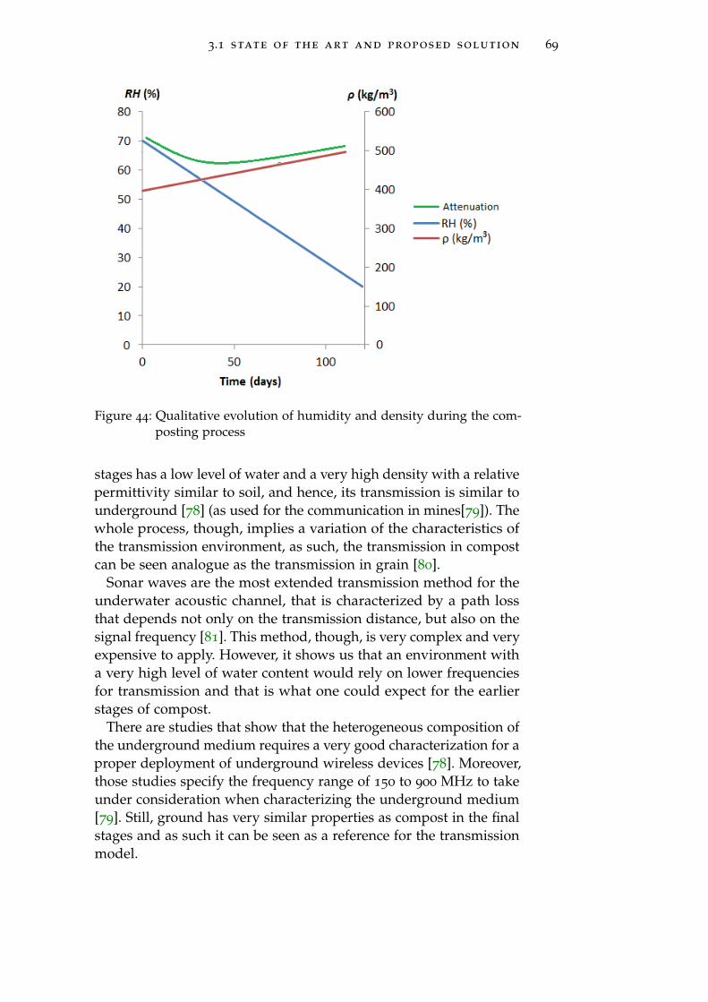
3.1 state of the art and proposed solution 69
Figure 44: Qualitative evolution of humidity and density during the com-posting process
stages has a low level of water and a very high density with a relativepermittivity similar to soil, and hence, its transmission is similar tounderground [78] (as used for the communication in mines[79]). Thewhole process, though, implies a variation of the characteristics ofthe transmission environment, as such, the transmission in compostcan be seen analogue as the transmission in grain [80].
Sonar waves are the most extended transmission method for theunderwater acoustic channel, that is characterized by a path lossthat depends not only on the transmission distance, but also on thesignal frequency [81]. This method, though, is very complex and veryexpensive to apply. However, it shows us that an environment witha very high level of water content would rely on lower frequenciesfor transmission and that is what one could expect for the earlierstages of compost.
There are studies that show that the heterogeneous composition ofthe underground medium requires a very good characterization for aproper deployment of underground wireless devices [78]. Moreover,those studies specify the frequency range of 150 to 900 MHz to takeunder consideration when characterizing the underground medium[79]. Still, ground has very similar properties as compost in the finalstages and as such it can be seen as a reference for the transmissionmodel.
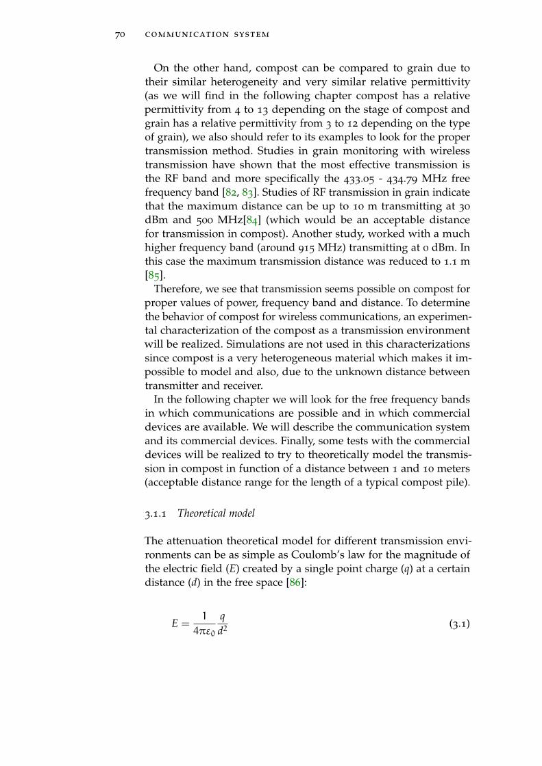
70 communication system
On the other hand, compost can be compared to grain due totheir similar heterogeneity and very similar relative permittivity(as we will find in the following chapter compost has a relativepermittivity from 4 to 13 depending on the stage of compost andgrain has a relative permittivity from 3 to 12 depending on the typeof grain), we also should refer to its examples to look for the propertransmission method. Studies in grain monitoring with wirelesstransmission have shown that the most effective transmission isthe RF band and more specifically the 433.05 - 434.79 MHz freefrequency band [82, 83]. Studies of RF transmission in grain indicatethat the maximum distance can be up to 10 m transmitting at 30
dBm and 500 MHz[84] (which would be an acceptable distancefor transmission in compost). Another study, worked with a muchhigher frequency band (around 915 MHz) transmitting at 0 dBm. Inthis case the maximum transmission distance was reduced to 1.1 m[85].
Therefore, we see that transmission seems possible on compost forproper values of power, frequency band and distance. To determinethe behavior of compost for wireless communications, an experimen-tal characterization of the compost as a transmission environmentwill be realized. Simulations are not used in this characterizationssince compost is a very heterogeneous material which makes it im-possible to model and also, due to the unknown distance betweentransmitter and receiver.
In the following chapter we will look for the free frequency bandsin which communications are possible and in which commercialdevices are available. We will describe the communication systemand its commercial devices. Finally, some tests with the commercialdevices will be realized to try to theoretically model the transmis-sion in compost in function of a distance between 1 and 10 meters(acceptable distance range for the length of a typical compost pile).
3.1.1 Theoretical model
The attenuation theoretical model for different transmission envi-ronments can be as simple as Coulomb’s law for the magnitude ofthe electric field (E) created by a single point charge (q) at a certaindistance (d) in the free space [86]:
E =1
4πε0
qd2
(3.1)
3.1 state of the art and proposed solution 71
or the simplified formula for the path loss (L) in the air for RFtransmission [13]
L (dB) = 20log(4πd
λ
)(3.2)
where d is the distance the wave travels and λ is the wavelength.or even as complex as the Okumura-Hata wireless communication
model for predicting the behavior of cellular transmissions in urbanareas. There, the path loss is
LU (dB) = 69.55+ 26.16log (f) − 13.82log (hB) − CH+
+ [44.9− 6.55log (hB)] log (d) (3.3)
where f is the transmission frequency in MHz, hB is the heightof the base station antenna, CH is the antenna height correctionfactor (also known as antenna factor) and d is the distance betweenthe base and mobile stations in km. As we can see, the higher thefrequency the higher the attenuation of the environment.
In the case of small or medium sized cities
CH = 0.8+ (1.1log (f) − 0.7)hM − 1.56log (f) (3.4)
and for large cities
CH =
8.29 (log (1.54hM))2 − 1.1, if 150 6 f 6 200
3.2 (log (11.75hM))2 − 4.97, if 200 < f 6 1500
(3.5)
where hM is the height of the mobile station antenna.This last model is suited for both point-to-point and broadcast
transmissions in urban areas and it is based on extensive empiricalmeasurements taken, and as such, it is very complex to apply to ourcase because the size of the antennas is really small. This impliesthat, according to this model (Equation 3.3) and considering anantenna of 1 m, our wave would attenuate at a minimum rateof 1/d4.49 approximately and would attenuate more for smallerantennas (1/d[4.49−0.655log(hB)]).
We stated that one of the most analogue studied material to trans-mission inside compost is grain together with ground. Hence, wewould expect compost to have a similar attenuation theoretical
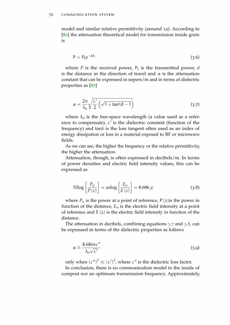
72 communication system
model and similar relative permittivity (around 12). According to[80] the attenuation theoretical model for transmission inside grainis
P = Pte−2d¸ (3.6)
where P is the received power, Pt is the transmitted power, dis the distance in the direction of travel and α is the attenuationconstant that can be expressed in nepers/m and in terms of dielectricproperties as [87]
α =2π
λo
√ε ′
2
(√1+ tan2d − 1
)(3.7)
where λo is the free-space wavelength (a value used as a refer-ence to compensate), ε ′ is the dielectric constant (function of thefrequency) and tanδ is the loss tangent often used as an index ofenergy dissipation or loss in a material exposed to RF or microwavefields.
As we can see, the higher the frequency or the relative permittivity,the higher the attenuation.
Attenuation, though, is often expressed in decibels/m. In termsof power densities and electric field intensity values, this can beexpressed as
10log[
Po
P (z)
]= 20log
[Eo
E (z)
]= 8.686¸z (3.8)
where Po is the power at a point of reference, P (z)is the power infunction of the distance, Eo is the electric field intensity at a pointof reference and E (z) is the electric field intensity in function of thedistance.
The attenuation in decibels, combining equations 3.7 and 3.8, canbe expressed in terms of the dielectric properties as follows
α ∼=8.686πε ′′
λo√ε ′
(3.9)
only when (ε ′′)2 (ε ′)2, where ε ′′ is the dielectric loss factor.In conclusion, there is no communication model in the inside of
compost nor an optimum transmission frequency. Approximately,

3.1 state of the art and proposed solution 73
air attenuates at a 1/d2 rate, grain attenuates at e−¸d
, and in a cityat 1/d4.49. There is a need for frequential characterization measuresfor compost which would be used to select the frequency and adjustthe behavior to one of the previous models.
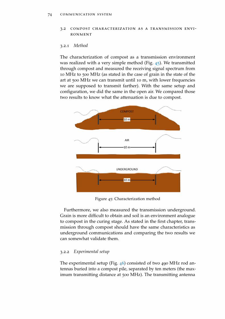
74 communication system
3.2 compost characterization as a transmission envi-ronment
3.2.1 Method
The characterization of compost as a transmission environmentwas realized with a very simple method (Fig. 45). We transmittedthrough compost and measured the receiving signal spectrum from10 MHz to 500 MHz (as stated in the case of grain in the state of theart at 500 MHz we can transmit until 10 m, with lower frequencieswe are supposed to transmit farther). With the same setup andconfiguration, we did the same in the open air. We compared thosetwo results to know what the attenuation is due to compost.
Figure 45: Characterization method
Furthermore, we also measured the transmission underground.Grain is more difficult to obtain and soil is an environment analogueto compost in the curing stage. As stated in the first chapter, trans-mission through compost should have the same characteristics asunderground communications and comparing the two results wecan somewhat validate them.
3.2.2 Experimental setup
The experimental setup (Fig. 46) consisted of two 490 MHz rod an-tennas buried into a compost pile, separated by ten meters (the max-imum transmitting distance at 500 MHz). The transmitting antenna
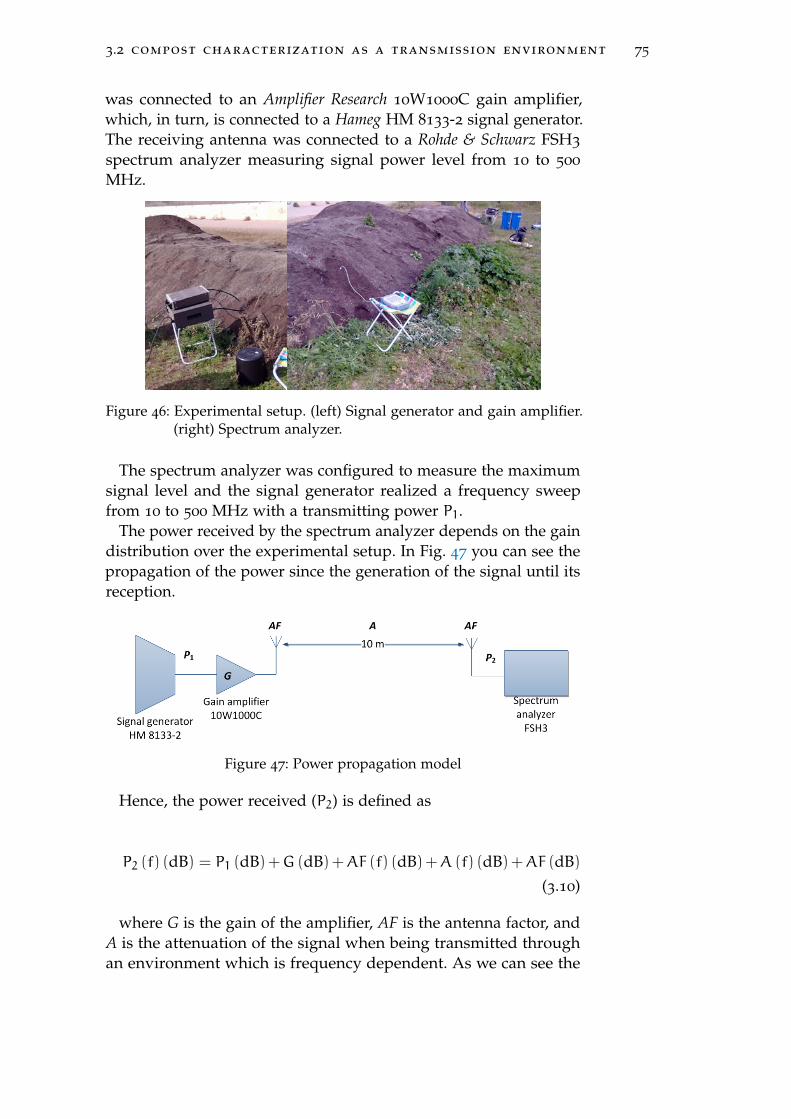
3.2 compost characterization as a transmission environment 75
was connected to an Amplifier Research 10W1000C gain amplifier,which, in turn, is connected to a Hameg HM 8133-2 signal generator.The receiving antenna was connected to a Rohde & Schwarz FSH3
spectrum analyzer measuring signal power level from 10 to 500
MHz.
Figure 46: Experimental setup. (left) Signal generator and gain amplifier.(right) Spectrum analyzer.
The spectrum analyzer was configured to measure the maximumsignal level and the signal generator realized a frequency sweepfrom 10 to 500 MHz with a transmitting power P1.
The power received by the spectrum analyzer depends on the gaindistribution over the experimental setup. In Fig. 47 you can see thepropagation of the power since the generation of the signal until itsreception.
Figure 47: Power propagation model
Hence, the power received (P2) is defined as
P2 (f) (dB) = P1 (dB)+G (dB)+AF (f) (dB)+A (f) (dB)+AF (dB)(3.10)
where G is the gain of the amplifier, AF is the antenna factor, andA is the attenuation of the signal when being transmitted throughan environment which is frequency dependent. As we can see the
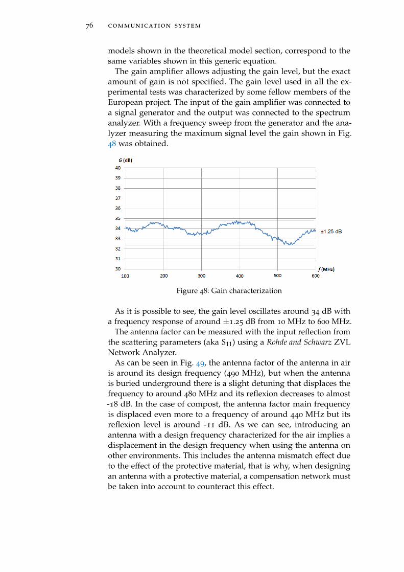
76 communication system
models shown in the theoretical model section, correspond to thesame variables shown in this generic equation.
The gain amplifier allows adjusting the gain level, but the exactamount of gain is not specified. The gain level used in all the ex-perimental tests was characterized by some fellow members of theEuropean project. The input of the gain amplifier was connected toa signal generator and the output was connected to the spectrumanalyzer. With a frequency sweep from the generator and the ana-lyzer measuring the maximum signal level the gain shown in Fig.48 was obtained.
Figure 48: Gain characterization
As it is possible to see, the gain level oscillates around 34 dB witha frequency response of around ±1.25 dB from 10 MHz to 600 MHz.
The antenna factor can be measured with the input reflection fromthe scattering parameters (aka S11) using a Rohde and Schwarz ZVLNetwork Analyzer.
As can be seen in Fig. 49, the antenna factor of the antenna in airis around its design frequency (490 MHz), but when the antennais buried underground there is a slight detuning that displaces thefrequency to around 480 MHz and its reflexion decreases to almost-18 dB. In the case of compost, the antenna factor main frequencyis displaced even more to a frequency of around 440 MHz but itsreflexion level is around -11 dB. As we can see, introducing anantenna with a design frequency characterized for the air implies adisplacement in the design frequency when using the antenna onother environments. This includes the antenna mismatch effect dueto the effect of the protective material, that is why, when designingan antenna with a protective material, a compensation network mustbe taken into account to counteract this effect.
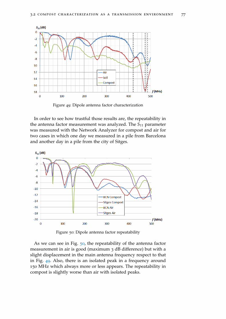
3.2 compost characterization as a transmission environment 77
Figure 49: Dipole antenna factor characterization
In order to see how trustful those results are, the repeatability inthe antenna factor measurement was analyzed. The S11 parameterwas measured with the Network Analyzer for compost and air fortwo cases in which one day we measured in a pile from Barcelonaand another day in a pile from the city of Sitges.
Figure 50: Dipole antenna factor repeatability
As we can see in Fig. 50, the repeatability of the antenna factormeasurement in air is good (maximum 3 dB difference) but with aslight displacement in the main antenna frequency respect to thatin Fig. 49. Also, there is an isolated peak in a frequency around150 MHz which always more or less appears. The repeatability incompost is slightly worse than air with isolated peaks.
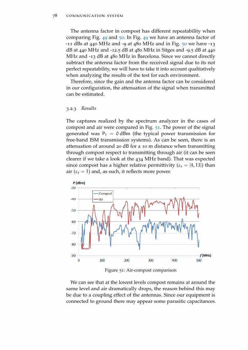
78 communication system
The antenna factor in compost has different repeatability whencomparing Fig. 49 and 50. In Fig. 49 we have an antenna factor of-11 dBs at 440 MHz and -9 at 480 MHz and in Fig. 50 we have -13
dB at 440 MHz and -12.5 dB at 480 MHz in Sitges and -9.5 dB at 440
MHz and -13 dB at 480 MHz in Barcelona. Since we cannot directlysubtract the antenna factor from the received signal due to its notperfect repeatability, we will have to take it into account qualitativelywhen analyzing the results of the test for each environment.
Therefore, since the gain and the antenna factor can be consideredin our configuration, the attenuation of the signal when transmittedcan be estimated.
3.2.3 Results
The captures realized by the spectrum analyzer in the cases ofcompost and air were compared in Fig. 51. The power of the signalgenerated was P1 = 0 dBm (the typical power transmission forfree-band ISM transmission systems). As can be seen, there is anattenuation of around 20 dB for a 10 m distance when transmittingthrough compost respect to transmitting through air (it can be seenclearer if we take a look at the 434 MHz band). That was expectedsince compost has a higher relative permittivity (εr = [4, 13]) thanair (εr = 1) and, as such, it reflects more power.
Figure 51: Air-compost comparison
We can see that at the lowest levels compost remains at around thesame level and air dramatically drops, the reason behind this maybe due to a coupling effect of the antennas. Since our equipment isconnected to ground there may appear some parasitic capacitances.
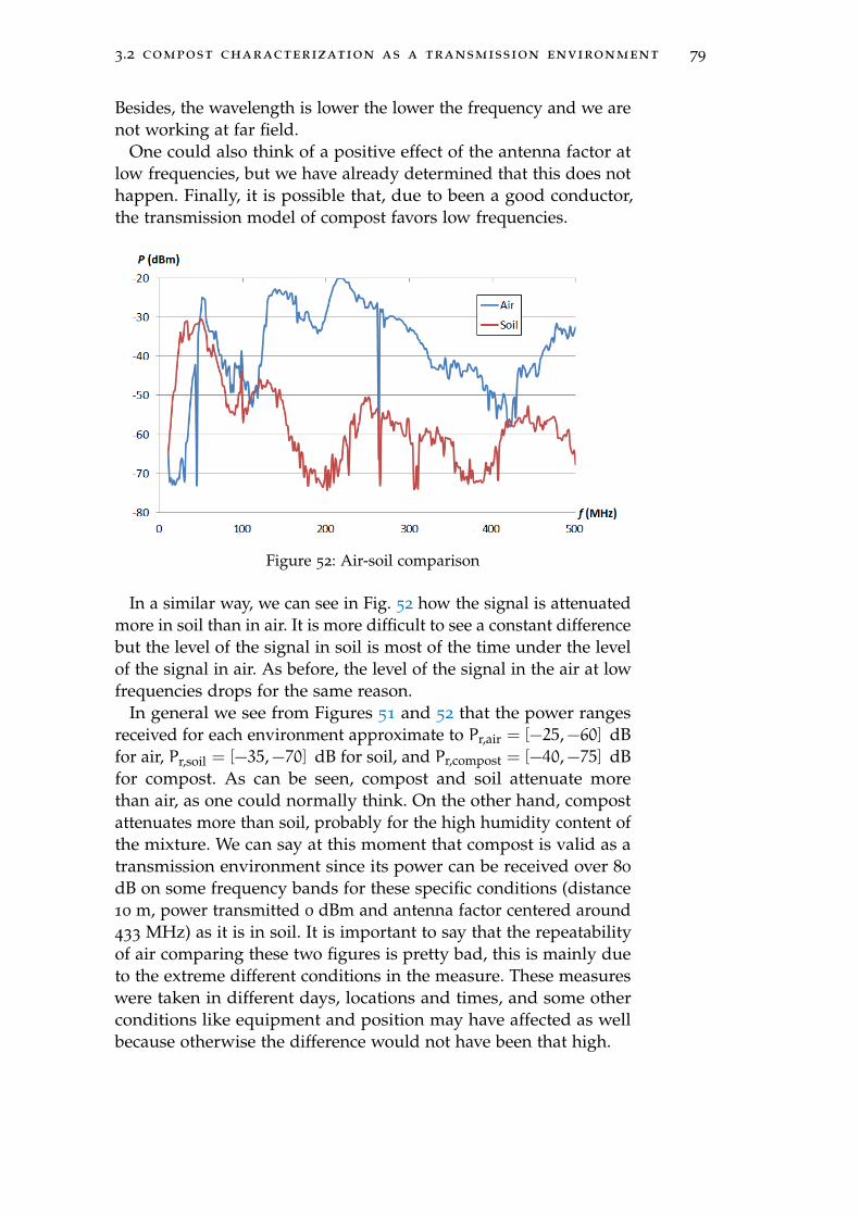
3.2 compost characterization as a transmission environment 79
Besides, the wavelength is lower the lower the frequency and we arenot working at far field.
One could also think of a positive effect of the antenna factor atlow frequencies, but we have already determined that this does nothappen. Finally, it is possible that, due to been a good conductor,the transmission model of compost favors low frequencies.
Figure 52: Air-soil comparison
In a similar way, we can see in Fig. 52 how the signal is attenuatedmore in soil than in air. It is more difficult to see a constant differencebut the level of the signal in soil is most of the time under the levelof the signal in air. As before, the level of the signal in the air at lowfrequencies drops for the same reason.
In general we see from Figures 51 and 52 that the power rangesreceived for each environment approximate to Pr,air = [−25,−60] dBfor air, Pr,soil = [−35,−70] dB for soil, and Pr,compost = [−40,−75] dBfor compost. As can be seen, compost and soil attenuate morethan air, as one could normally think. On the other hand, compostattenuates more than soil, probably for the high humidity content ofthe mixture. We can say at this moment that compost is valid as atransmission environment since its power can be received over 80
dB on some frequency bands for these specific conditions (distance10 m, power transmitted 0 dBm and antenna factor centered around433 MHz) as it is in soil. It is important to say that the repeatabilityof air comparing these two figures is pretty bad, this is mainly dueto the extreme different conditions in the measure. These measureswere taken in different days, locations and times, and some otherconditions like equipment and position may have affected as wellbecause otherwise the difference would not have been that high.
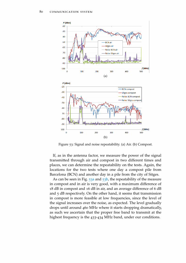
80 communication system
(a)
(b)
Figure 53: Signal and noise repeatability. (a) Air. (b) Compost.
If, as in the antenna factor, we measure the power of the signaltransmitted through air and compost in two different times andplaces, we can determine the repeatability on the tests. Again, thelocations for the two tests where one day a compost pile fromBarcelona (BCN) and another day in a pile from the city of Sitges.
As can be seen in Fig. 53a and 53b, the repeatability of the measurein compost and in air is very good, with a maximum difference of18 dB in compost and 16 dB in air, and an average difference of 6 dBand 5 dB respectively. On the other hand, it seems that transmissionin compost is more feasible at low frequencies, since the level ofthe signal increases over the noise, as expected. The level graduallydrops until around 460 MHz where it starts dropping dramatically,as such we ascertain that the proper free band to transmit at thehighest frequency is the 433-434 MHz band, under our conditions.
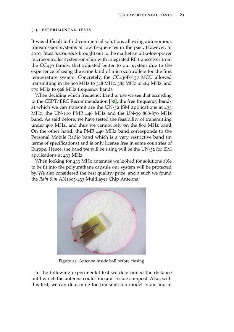
3.3 experimental tests 81
3.3 experimental tests
It was difficult to find commercial solutions allowing autonomoustransmission systems at low frequencies in the past. However, in2010, Texas Instruments brought out to the market an ultra-low-powermicrocontroller system-on-chip with integrated RF transceiver fromthe CC430 family, that adjusted better to our system due to theexperience of using the same kind of microcontrollers for the firsttemperature system. Concretely, the CC430F6137 MCU allowedtransmitting in the 300 MHz to 348 MHz, 389 MHz to 464 MHz, and779 MHz to 928 MHz frequency bands.
When deciding which frequency band to use we see that accordingto the CEPT/ERC Recommendation [88], the free frequency bandsat which we can transmit are the UN-32 ISM applications at 433
MHz, the UN-110 PMR 446 MHz and the UN-39 868-870 MHzband. As said before, we have tested the feasibility of transmittingunder 460 MHz, and thus we cannot rely on the 800 MHz band.On the other hand, the PMR 446 MHz band corresponds to thePersonal Mobile Radio band which is a very restrictive band (interms of specifications) and is only license free in some countries ofEurope. Hence, the band we will be using will be the UN-32 for ISMapplications at 433 MHz.
When looking for 433 MHz antennas we looked for solutions ableto be fit into the polyurethane capsule our system will be protectedby. We also considered the best quality/prize, and a such we foundthe Rain Sun AN1603-433 Multilayer Chip Antenna.
Figure 54: Antenna inside ball before closing
In the following experimental test we determined the distanceuntil which the antenna could transmit inside compost. Also, withthis test, we can determine the transmission model in air and in
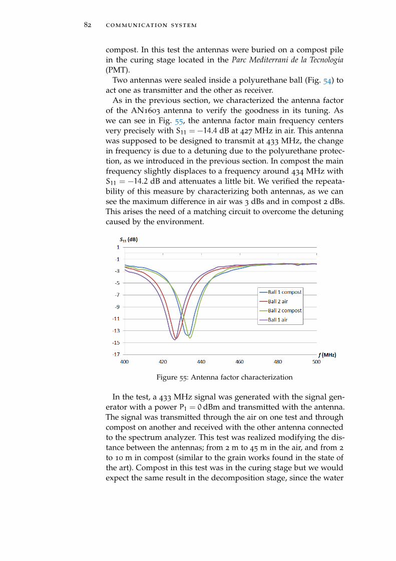
82 communication system
compost. In this test the antennas were buried on a compost pilein the curing stage located in the Parc Mediterrani de la Tecnologia(PMT).
Two antennas were sealed inside a polyurethane ball (Fig. 54) toact one as transmitter and the other as receiver.
As in the previous section, we characterized the antenna factorof the AN1603 antenna to verify the goodness in its tuning. Aswe can see in Fig. 55, the antenna factor main frequency centersvery precisely with S11 = −14.4 dB at 427 MHz in air. This antennawas supposed to be designed to transmit at 433 MHz, the changein frequency is due to a detuning due to the polyurethane protec-tion, as we introduced in the previous section. In compost the mainfrequency slightly displaces to a frequency around 434 MHz withS11 = −14.2 dB and attenuates a little bit. We verified the repeata-bility of this measure by characterizing both antennas, as we cansee the maximum difference in air was 3 dBs and in compost 2 dBs.This arises the need of a matching circuit to overcome the detuningcaused by the environment.
Figure 55: Antenna factor characterization
In the test, a 433 MHz signal was generated with the signal gen-erator with a power P1 = 0 dBm and transmitted with the antenna.The signal was transmitted through the air on one test and throughcompost on another and received with the other antenna connectedto the spectrum analyzer. This test was realized modifying the dis-tance between the antennas; from 2 m to 45 m in the air, and from 2
to 10 m in compost (similar to the grain works found in the state ofthe art). Compost in this test was in the curing stage but we wouldexpect the same result in the decomposition stage, since the water
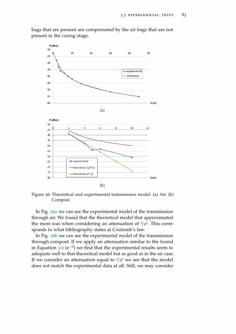
3.3 experimental tests 83
bags that are present are compensated by the air bags that are notpresent in the curing stage.
(a)
(b)
Figure 56: Theoretical and experimental transmission model. (a) Air. (b)Compost.
In Fig. 56a we can see the experimental model of the transmissionthrough air. We found that the theoretical model that approximatedthe most was when considering an attenuation of 1/d2. This corre-sponds to what bibliography states at Coulomb’s law.
In Fig. 56b we can see the experimental model of the transmissionthrough compost. If we apply an attenuation similar to the foundin Equation 3.6 (e−d) we find that the experimental results seem toadequate well to that theoretical model but as good as in the air case.If we consider an attenuation equal to 1/d2 we see that the modeldoes not match the experimental data at all. Still, we may consider
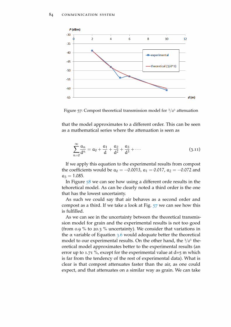
84 communication system
Figure 57: Compost theoretical transmission model for 1/d3 attenuation
that the model approximates to a different order. This can be seenas a mathematical series where the attenuation is seen as
∞∑n=0
an
dn= a0 +
a1d
+a2d2
+a3d3
+ · · · (3.11)
If we apply this equation to the experimental results from compostthe coefficients would be a0 = −0.0013, a1 = 0.017, a2 = −0.072 anda3 = 1.085.
In Figure 58 we can see how using a different orde results in thetehoretical model. As can be clearly noted a third order is the onethat has the lowest uncertainty.
As such we could say that air behaves as a second order andcompost as a third. If we take a look at Fig. 57 we can see how thisis fulfilled.
As we can see in the uncertainty between the theoretical transmis-sion model for grain and the experimental results is not too good(from 0.9 % to 20.3 % uncertainty). We consider that variations inthe α variable of Equation 3.6 would adequate better the theoreticalmodel to our experimental results. On the other hand, the 1/d3 the-oretical model approximates better to the experimental results (anerror up to 1.71 %, except for the experimental value at d=5 m whichis far from the tendency of the rest of experimental data). What isclear is that compost attenuates faster than the air, as one couldexpect, and that attenuates on a similar way as grain. We can take
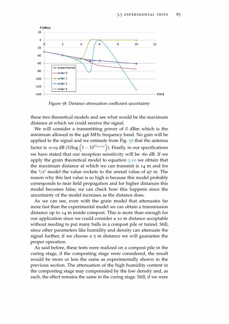
3.3 experimental tests 85
Figure 58: Distance attenuation coefficient uncertainty
these two theoretical models and see what would be the maximumdistance at which we could receive the signal.
We will consider a transmitting power of 0 dBm which is theminimum allowed in the 446 MHz frequency band. No gain will beapplied to the signal and we estimate from Fig. 55 that the antennafactor is -0.19 dB (10log
(1− 10(S11/10)
)). Finally, in our specifications
we have stated that our reception sensitivity will be -60 dB. If weapply the grain theoretical model to equation 3.10 we obtain thatthe maximum distance at which we can transmit is 14 m and forthe 1/d3 model the value rockets to the unreal value of 97 m. Thereason why this last value is so high is because this model probablycorresponds to near field propagation and for higher distances thismodel becomes false; we can check how this happens since theuncertainty of the model increases as the distance does.
As we can see, even with the grain model that attenuates farmore fast than the experimental model we can obtain a transmissiondistance up to 14 m inside compost. This is more than enough forour application since we could consider a 10 m distance acceptablewithout needing to put many balls in a compost pile or tunnel. Still,since other parameters like humidity and density can attenuate thesignal further, if we choose a 5 m distance we will guarantee theproper operation.
As said before, these tests were realized on a compost pile in thecuring stage, if the composting stage were considered, the resultwould be more or less the same as experimentally shown in theprevious section. The attenuation of the high humidity content inthe composting stage may compensated by the low density and, assuch, the effect remains the same in the curing stage. Still, if we were

86 communication system
interested in having a larger transmission distance, we could alwaysconcatenate transmission systems developing a sensor network.
This kind of network has been implemented within the Compo-ball project (http://www.compoball.eu/) and its operation has beendemonstrated for distances until 4 m in conditions of high humiditycontent.
In front of so many imbecils with opinion card,wise men don’t talk.
— Pepe Rubianes, comedian
4H U M I D I T Y S Y S T E M
4.1 state of the art and proposed solution
To monitor humidity during the composting process, a commonway is extracting samples to analyze at a laboratory, with the eco-nomical and temporal cost it supposes. Another way of measuringthe moisture content of compost is using probes as in temperature[89], but these probes cannot be continuously measuring due tothe degradation that supposes to be in contact with the compostmaterial, and their high cost [90].
There are already contact-less solutions that measure moisturecontent in compost through microwave attenuation [91, 92] insidecapsules as in the temperature system. This may be a good solutionbut high frequency systems result on a considerable increase ofthe cost and the high water content makes transmission costly inconsumption terms. Therefore using lower frequencies would bebetter in order to reduce consumption, as proposed during theprevious chapter.
Another very extended and old solution in the contact-less mea-sure of humidity is using coplanar capacitive electrodes [93]. Thissolution relies on the shape and dimensions of the electrodes to op-timize the humidity measurement. The most famous shape throughhistory for coplanar capacitive electrodes is the interdigital electrodedesign, the earliest example is found in the patent of N. Tesla in1891 [94]. And its theoretical expressions for calculation of theircapacitance appeared in the 20s [95]. The expanded use of coplanarinterdigital electrodes was found in the 60s [96] along with other elec-trode shapes [97]. But their commercialization did not start until the80s [98] and 90s [99] in the United States. Many examples, old andnew, of coplanar interdigital electrodes in the measure of moisturecan be found [100, 101]. And a lot of research based on their per-formance has been realized; as on their use as capacitive, inductive,
87
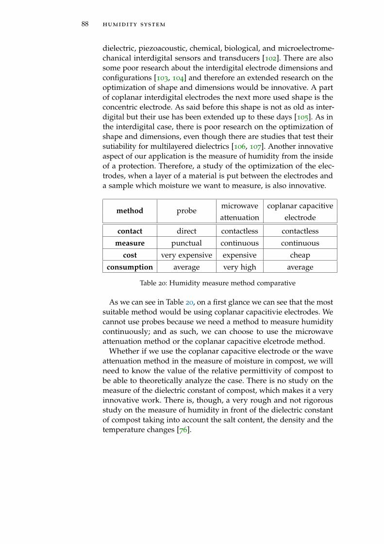
88 humidity system
dielectric, piezoacoustic, chemical, biological, and microelectrome-chanical interdigital sensors and transducers [102]. There are alsosome poor research about the interdigital electrode dimensions andconfigurations [103, 104] and therefore an extended research on theoptimization of shape and dimensions would be innovative. A partof coplanar interdigital electrodes the next more used shape is theconcentric electrode. As said before this shape is not as old as inter-digital but their use has been extended up to these days [105]. As inthe interdigital case, there is poor research on the optimization ofshape and dimensions, even though there are studies that test theirsutiability for multilayered dielectrics [106, 107]. Another innovativeaspect of our application is the measure of humidity from the insideof a protection. Therefore, a study of the optimization of the elec-trodes, when a layer of a material is put between the electrodes anda sample which moisture we want to measure, is also innovative.
method probemicrowave coplanar capacitiveattenuation electrode
contact direct contactless contactless
measure punctual continuous continuous
cost very expensive expensive cheap
consumption average very high average
Table 20: Humidity measure method comparative
As we can see in Table 20, on a first glance we can see that the mostsuitable method would be using coplanar capacitivie electrodes. Wecannot use probes because we need a method to measure humiditycontinuously; and as such, we can choose to use the microwaveattenuation method or the coplanar capacitive elcetrode method.
Whether if we use the coplanar capacitive electrode or the waveattenuation method in the measure of moisture in compost, we willneed to know the value of the relative permittivity of compost tobe able to theoretically analyze the case. There is no study on themeasure of the dielectric constant of compost, which makes it a veryinnovative work. There is, though, a very rough and not rigorousstudy on the measure of humidity in front of the dielectric constantof compost taking into account the salt content, the density and thetemperature changes [76].
4.1 state of the art and proposed solution 89
4.1.1 Proposed solution
We want to obtain a method to measure humidity from the insideof a protection, from which the state of the art has shown twopossibilities: coplanar capacitive electrodes or wave attenuation.
Humidity monitoring through the measure of wave attenuationinside compost consists of a node transmitting a signal to a receivingnode where this one calculates the humidity with the attenuation ofthe wave in front of the distance between the nodes. This scenariodoes not have a clear theoretical background due to its complexity,but we can use simulation programs to theoretically analyze it. Oneof the problems of this method is the need to know the location of theballs to calculate the distance between them, which is very complex.Another way to know the distance between nodes would be usingtwo or more training signals at different frequencies which will bedifferently attenuated and therefore the distance can be calculated.The problem of this solution is the need of a bigger transmissionsystem, which is not only a problem in terms of dimensions butalso would imply an even higher power consumption. There is ageneral problem with this method and that is the lost balls due tothe action of the compost turner, as said in section 2.4.1; if thereare balls outside the compost pile the calculation of the distancebecomes wrong and hence the method cannot be used. Furthermore,as show in the previous chapter, the orientation of the antenna inthe communication system is critical if we want to transmit betweentwo nodes.
The humidity monitoring through the use of coplanar capacitiveelectrodes consists of a pair of electrodes inside a ball emitting anelectric field that is affected by the material it goes through (Fig. 59).Although coplanar capacitive electrodes do have theoretical models,the scenario results more complex and thus these models cannot beused. Hence, a simulation software should be used to theoreticallyanalyze this method, just like in the previous one. In this case, thereis no problem with the location of the balls: if it is inside the pile itwill measure, if not, it will not; there is nothing else about it. But thegreatest advantage of this method has in front of the previous one ispower consumption; we are developing an autonomous system and,as such, this factor is critical.
Therefore we will develop a humidity sensor system based on thechanges of a pair of coplanar capacitive electrodes placed insidea capsule. The humidity system will have the same specificationsof the temperature system (Chapter 2) but with the change thatthe maximum required accuracy of this system will be of a ±5
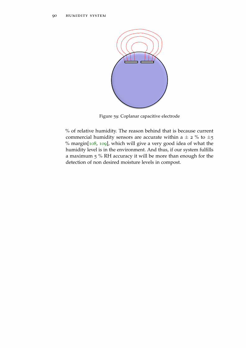
90 humidity system
Figure 59: Coplanar capacitive electrode
% of relative humidity. The reason behind that is because currentcommercial humidity sensors are accurate within a ± 2 % to ±5
% margin[108, 109], which will give a very good idea of what thehumidity level is in the environment. And thus, if our system fulfillsa maximum 5 % RH accuracy it will be more than enough for thedetection of non desired moisture levels in compost.
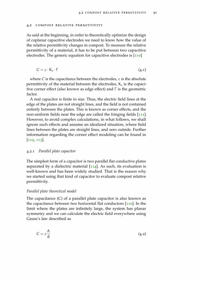
4.2 compost relative permittivity 91
4.2 compost relative permittivity
As said at the beginning, in order to theoretically optimize the designof coplanar capacitive electrodes we need to know how the value ofthe relative permittivity changes in compost. To measure the relativepermittivity of a material, it has to be put between two capacitiveelectrodes. The generic equation for capacitive electrodes is [110]
C = ε ·Kc · Γ (4.1)
where C is the capacitance between the electrodes, ε is the absolutepermittivity of the material between the electrodes, Kc is the capaci-tive corner effect (also known as edge effect) and Γ is the geometricfactor.
A real capacitor is finite in size. Thus, the electric field lines at theedge of the plates are not straight lines, and the field is not containedentirely between the plates. This is known as corner effects, and thenon-uniform fields near the edge are called the fringing fields [111].However, to avoid complex calculations, in what follows, we shallignore such effects and assume an idealized situation, where fieldlines between the plates are straight lines, and zero outside. Furtherinformation regarding the corner effect modeling can be found in[112, 113].
4.2.1 Parallel plate capacitor
The simplest form of a capacitor is two parallel flat conductive platesseparated by a dielectric material [114]. As such, its evaluation iswell-known and has been widely studied. That is the reason whywe started using that kind of capacitor to evaluate compost relativepermittivity.
Parallel plate theoretical model
The capacitance (C) of a parallel plate capacitor is also known asthe capacitance between two horizontal flat conductors [110]. In thelimit where the plates are infinitely large, the system has planarsymmetry and we can calculate the electric field everywhere usingGauss’s law described as
C = εA
d(4.2)
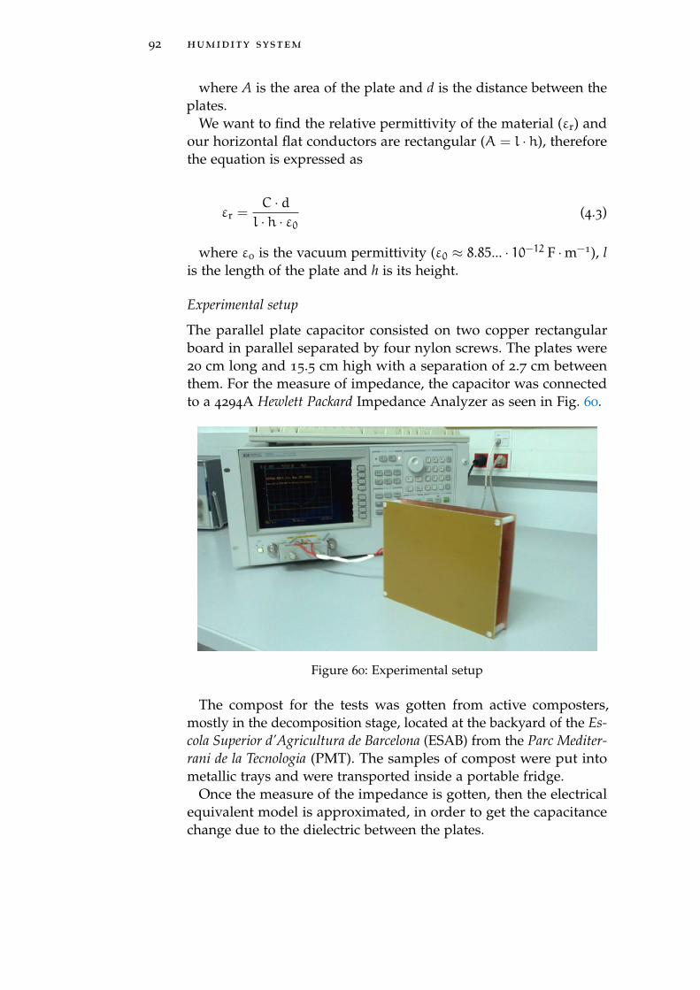
92 humidity system
where A is the area of the plate and d is the distance between theplates.
We want to find the relative permittivity of the material (εr) andour horizontal flat conductors are rectangular (A = l · h), thereforethe equation is expressed as
εr =C · dl · h · ε0
(4.3)
where ε0 is the vacuum permittivity (ε0 ≈ 8.85... · 10−12 F ·m−1), lis the length of the plate and h is its height.
Experimental setup
The parallel plate capacitor consisted on two copper rectangularboard in parallel separated by four nylon screws. The plates were20 cm long and 15.5 cm high with a separation of 2.7 cm betweenthem. For the measure of impedance, the capacitor was connectedto a 4294A Hewlett Packard Impedance Analyzer as seen in Fig. 60.
Figure 60: Experimental setup
The compost for the tests was gotten from active composters,mostly in the decomposition stage, located at the backyard of the Es-cola Superior d’Agricultura de Barcelona (ESAB) from the Parc Mediter-rani de la Tecnologia (PMT). The samples of compost were put intometallic trays and were transported inside a portable fridge.
Once the measure of the impedance is gotten, then the electricalequivalent model is approximated, in order to get the capacitancechange due to the dielectric between the plates.
4.2 compost relative permittivity 93
Results and discussion
We needed to find the electrical equivalent model for the measure ofcapacitance of the parallel plates with compost. With the theoreticalelectric model we can extract the values of the components (includ-ing the capacitance due to the dielectric between the plates) of themodel that suit it to the experimental result. We have done that bytaking the experimental data and introducing it to a Matlab R2011aalgorithm that found the values that got the nearest theoreticalimpedance module to the experimental one.
For that we started from the basic model which corresponds to theparallel plates with air. The corresponding model is an RC parallelor serial (in this case we applied the parallel one) with the inductiveeffect of the cables (serial inductances), as is demonstrated in Fig.61. Values for the equivalent theoretical parallel resistance, parallelcapacitance and cable inductance are Rp = 29.10 k˙, Cp = 18.64 pF,L = 0.19 —H respectively.
Figure 61: Electric equivalent model of the parallel plates with air
We applied this electric model to the plates filled with compost andwe obtained that the RC serial model does not suit our configurationwhilst the RC parallel model suits high frequencies (Fig. 62 with R =
39.17 ˙, C = 0.14 nF, L = 0.19 —H), except for some disturbances inthe measure at the highest frequencies. The mechanism responsiblefor the dispersion is equivalent to a complex impedance with aphase angle [115] which depends on the kind of dielectric we aretesting.
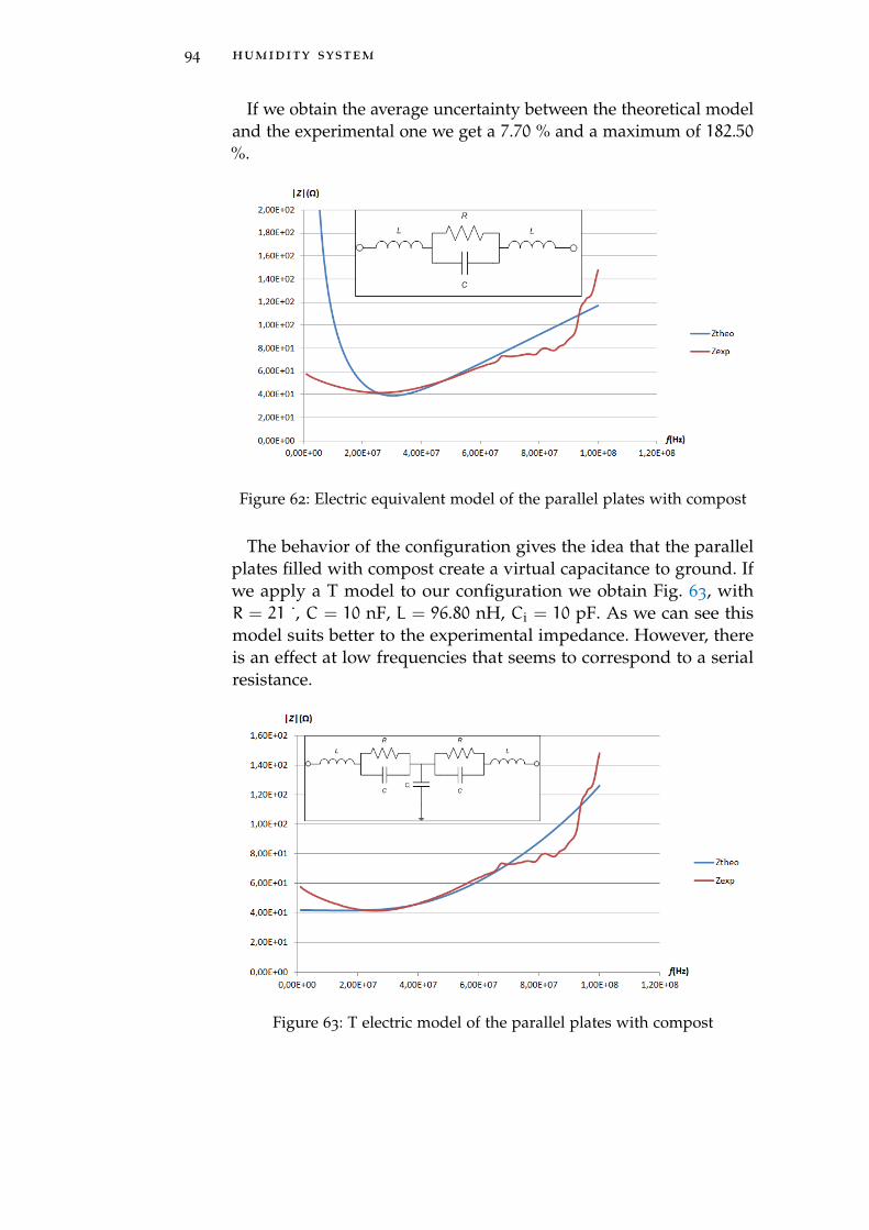
94 humidity system
If we obtain the average uncertainty between the theoretical modeland the experimental one we get a 7.70 % and a maximum of 182.50%.
Figure 62: Electric equivalent model of the parallel plates with compost
The behavior of the configuration gives the idea that the parallelplates filled with compost create a virtual capacitance to ground. Ifwe apply a T model to our configuration we obtain Fig. 63, withR = 21 ˙, C = 10 nF, L = 96.80 nH, Ci = 10 pF. As we can see thismodel suits better to the experimental impedance. However, thereis an effect at low frequencies that seems to correspond to a serialresistance.
Figure 63: T electric model of the parallel plates with compost
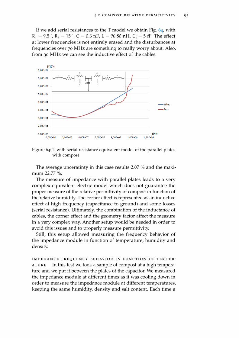
4.2 compost relative permittivity 95
If we add serial resistances to the T model we obtain Fig. 64, withR1 = 9.5 ˙, R2 = 15 ˙, C = 0.3 nF, L = 96.80 nH, Ci = 5 fF. The effectat lower frequencies is not entirely erased and the disturbances atfrequencies over 70 MHz are something to really worry about. Also,from 30 MHz we can see the inductive effect of the cables.
Figure 64: T with serial resistance equivalent model of the parallel plateswith compost
The average unceratinty in this case results 2.07 % and the maxi-mum 22.77 %.
The measure of impedance with parallel plates leads to a verycomplex equivalent electric model which does not guarantee theproper measure of the relative permittivity of compost in function ofthe relative humidity. The corner effect is represented as an inductiveeffect at high frequency (capacitance to ground) and some losses(serial resistance). Ultimately, the combination of the inductance ofcables, the corner effect and the geometry factor affect the measurein a very complex way. Another setup would be needed in order toavoid this issues and to properly measure permittivity.
Still, this setup allowed measuring the frequency behavior ofthe impedance module in function of temperature, humidity anddensity.
impedance frequency behavior in function of temper-ature In this test we took a sample of compost at a high tempera-ture and we put it between the plates of the capacitor. We measuredthe impedance module at different times as it was cooling down inorder to measure the impedance module at different temperatures,keeping the same humidity, density and salt content. Each time a
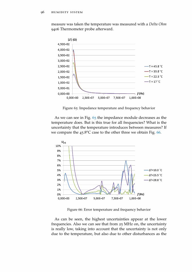
96 humidity system
measure was taken the temperature was measured with a Delta Ohm9406 Thermometer probe afterward.
Figure 65: Impedance temperature and frequency behavior
As we can see in Fig. 65 the impedance module decreases as thetemperature does. But is this true for all frequencies? What is theuncertainty that the temperature introduces between measures? Ifwe compare the 45.8oC case to the other three we obtain Fig. 66.
Figure 66: Error temperature and frequency behavior
As can be seen, the highest uncertainties appear at the lowerfrequencies. Also we can see that from 25 MHz on, the uncertaintyis really low, taking into account that the uncertainty is not onlydue to the temperature, but also due to other disturbances as the
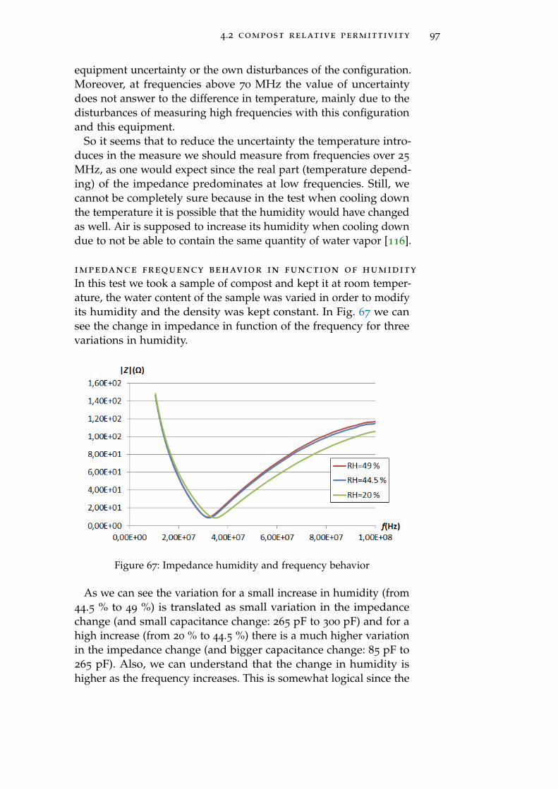
4.2 compost relative permittivity 97
equipment uncertainty or the own disturbances of the configuration.Moreover, at frequencies above 70 MHz the value of uncertaintydoes not answer to the difference in temperature, mainly due to thedisturbances of measuring high frequencies with this configurationand this equipment.
So it seems that to reduce the uncertainty the temperature intro-duces in the measure we should measure from frequencies over 25
MHz, as one would expect since the real part (temperature depend-ing) of the impedance predominates at low frequencies. Still, wecannot be completely sure because in the test when cooling downthe temperature it is possible that the humidity would have changedas well. Air is supposed to increase its humidity when cooling downdue to not be able to contain the same quantity of water vapor [116].
impedance frequency behavior in function of humidity
In this test we took a sample of compost and kept it at room temper-ature, the water content of the sample was varied in order to modifyits humidity and the density was kept constant. In Fig. 67 we cansee the change in impedance in function of the frequency for threevariations in humidity.
Figure 67: Impedance humidity and frequency behavior
As we can see the variation for a small increase in humidity (from44.5 % to 49 %) is translated as small variation in the impedancechange (and small capacitance change: 265 pF to 300 pF) and for ahigh increase (from 20 % to 44.5 %) there is a much higher variationin the impedance change (and bigger capacitance change: 85 pF to265 pF). Also, we can understand that the change in humidity ishigher as the frequency increases. This is somewhat logical since the
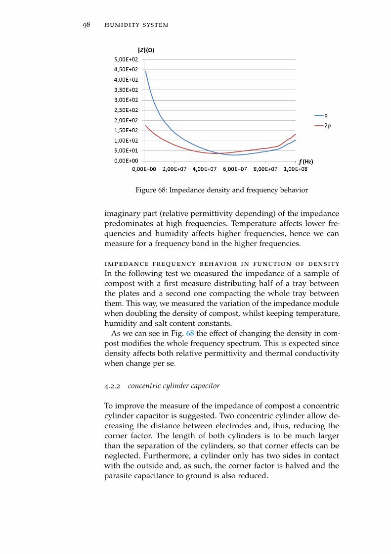
98 humidity system
Figure 68: Impedance density and frequency behavior
imaginary part (relative permittivity depending) of the impedancepredominates at high frequencies. Temperature affects lower fre-quencies and humidity affects higher frequencies, hence we canmeasure for a frequency band in the higher frequencies.
impedance frequency behavior in function of density
In the following test we measured the impedance of a sample ofcompost with a first measure distributing half of a tray betweenthe plates and a second one compacting the whole tray betweenthem. This way, we measured the variation of the impedance modulewhen doubling the density of compost, whilst keeping temperature,humidity and salt content constants.
As we can see in Fig. 68 the effect of changing the density in com-post modifies the whole frequency spectrum. This is expected sincedensity affects both relative permittivity and thermal conductivitywhen change per se.
4.2.2 concentric cylinder capacitor
To improve the measure of the impedance of compost a concentriccylinder capacitor is suggested. Two concentric cylinder allow de-creasing the distance between electrodes and, thus, reducing thecorner factor. The length of both cylinders is to be much largerthan the separation of the cylinders, so that corner effects can beneglected. Furthermore, a cylinder only has two sides in contactwith the outside and, as such, the corner factor is halved and theparasite capacitance to ground is also reduced.
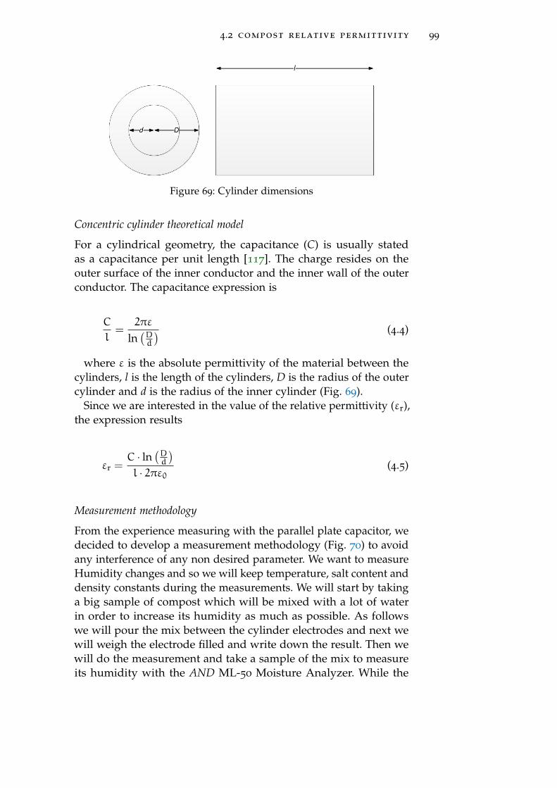
4.2 compost relative permittivity 99
Figure 69: Cylinder dimensions
Concentric cylinder theoretical model
For a cylindrical geometry, the capacitance (C) is usually statedas a capacitance per unit length [117]. The charge resides on theouter surface of the inner conductor and the inner wall of the outerconductor. The capacitance expression is
C
l=
2πε
ln(Dd
) (4.4)
where ε is the absolute permittivity of the material between thecylinders, l is the length of the cylinders, D is the radius of the outercylinder and d is the radius of the inner cylinder (Fig. 69).
Since we are interested in the value of the relative permittivity (εr),the expression results
εr =C · ln
(Dd
)l · 2πε0
(4.5)
Measurement methodology
From the experience measuring with the parallel plate capacitor, wedecided to develop a measurement methodology (Fig. 70) to avoidany interference of any non desired parameter. We want to measureHumidity changes and so we will keep temperature, salt content anddensity constants during the measurements. We will start by takinga big sample of compost which will be mixed with a lot of waterin order to increase its humidity as much as possible. As followswe will pour the mix between the cylinder electrodes and next wewill weigh the electrode filled and write down the result. Then wewill do the measurement and take a sample of the mix to measureits humidity with the AND ML-50 Moisture Analyzer. While the
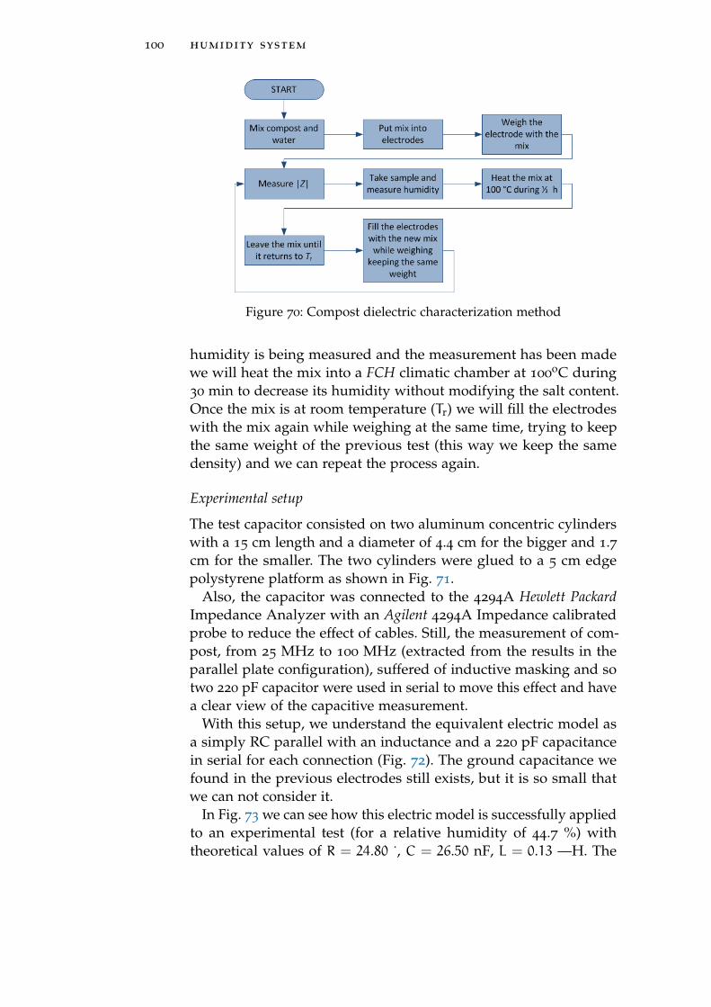
100 humidity system
Figure 70: Compost dielectric characterization method
humidity is being measured and the measurement has been madewe will heat the mix into a FCH climatic chamber at 100
oC during30 min to decrease its humidity without modifying the salt content.Once the mix is at room temperature (Tr) we will fill the electrodeswith the mix again while weighing at the same time, trying to keepthe same weight of the previous test (this way we keep the samedensity) and we can repeat the process again.
Experimental setup
The test capacitor consisted on two aluminum concentric cylinderswith a 15 cm length and a diameter of 4.4 cm for the bigger and 1.7cm for the smaller. The two cylinders were glued to a 5 cm edgepolystyrene platform as shown in Fig. 71.
Also, the capacitor was connected to the 4294A Hewlett PackardImpedance Analyzer with an Agilent 4294A Impedance calibratedprobe to reduce the effect of cables. Still, the measurement of com-post, from 25 MHz to 100 MHz (extracted from the results in theparallel plate configuration), suffered of inductive masking and sotwo 220 pF capacitor were used in serial to move this effect and havea clear view of the capacitive measurement.
With this setup, we understand the equivalent electric model asa simply RC parallel with an inductance and a 220 pF capacitancein serial for each connection (Fig. 72). The ground capacitance wefound in the previous electrodes still exists, but it is so small thatwe can not consider it.
In Fig. 73 we can see how this electric model is successfully appliedto an experimental test (for a relative humidity of 44.7 %) withtheoretical values of R = 24.80 ˙, C = 26.50 nF, L = 0.13 —H. The
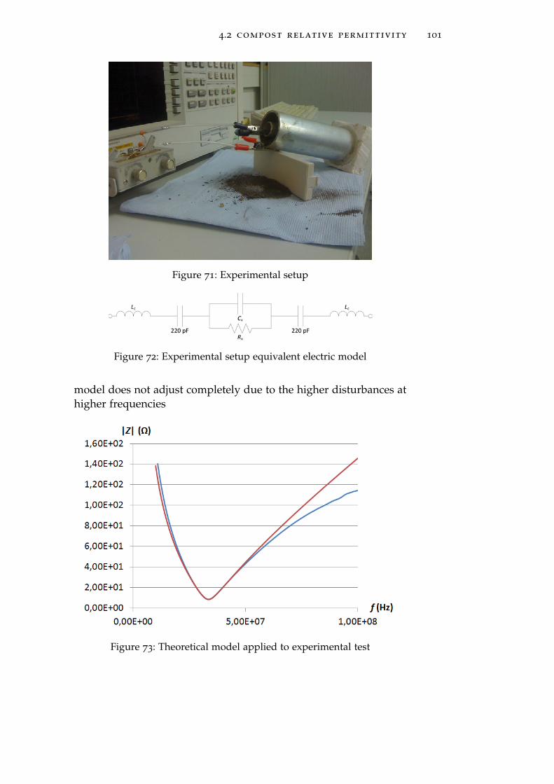
4.2 compost relative permittivity 101
Figure 71: Experimental setup
Figure 72: Experimental setup equivalent electric model
model does not adjust completely due to the higher disturbances athigher frequencies
Figure 73: Theoretical model applied to experimental test
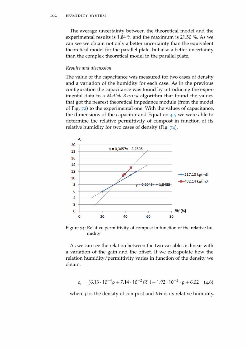
102 humidity system
The average uncertainty between the theoretical model and theexperimental results is 1.84 % and the maximum is 21.50 %. As wecan see we obtain not only a better uncertainty than the equivalenttheoretical model for the parallel plate, but also a better uncertaintythan the complex theoretical model in the parallel plate.
Results and discussion
The value of the capacitance was measured for two cases of densityand a variation of the humidity for each case. As in the previousconfiguration the capacitance was found by introducing the exper-imental data to a Matlab R2011a algorithm that found the valuesthat got the nearest theoretical impedance module (from the modelof Fig. 72) to the experimental one. With the values of capacitance,the dimensions of the capacitor and Equation 4.5 we were able todetermine the relative permittivity of compost in function of itsrelative humidity for two cases of density (Fig. 74).
Figure 74: Relative permittivity of compost in function of the relative hu-midity
As we can see the relation between the two variables is linear witha variation of the gain and the offset. If we extrapolate how therelation humidity/permittivity varies in function of the density weobtain:
εr = (6.13 · 10−4ρ+ 7.14 · 10−2)RH− 1.92 · 10−2 · ρ+ 6.02 (4.6)
where ρ is the density of compost and RH is its relative humidity.
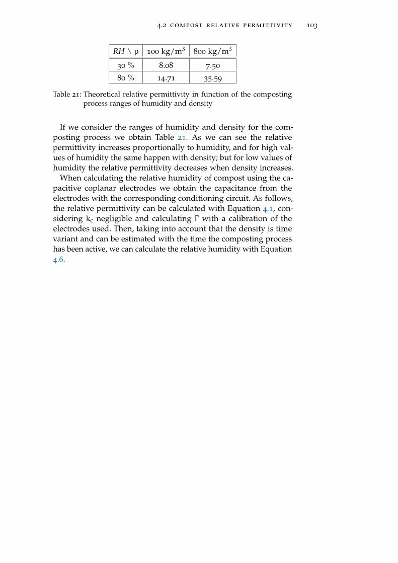
4.2 compost relative permittivity 103
RH \ ρ 100 kg/m3800 kg/m3
30 % 8.08 7.50
80 % 14.71 35.59
Table 21: Theoretical relative permittivity in function of the compostingprocess ranges of humidity and density
If we consider the ranges of humidity and density for the com-posting process we obtain Table 21. As we can see the relativepermittivity increases proportionally to humidity, and for high val-ues of humidity the same happen with density; but for low values ofhumidity the relative permittivity decreases when density increases.
When calculating the relative humidity of compost using the ca-pacitive coplanar electrodes we obtain the capacitance from theelectrodes with the corresponding conditioning circuit. As follows,the relative permittivity can be calculated with Equation 4.1, con-sidering kc negligible and calculating Γ with a calibration of theelectrodes used. Then, taking into account that the density is timevariant and can be estimated with the time the composting processhas been active, we can calculate the relative humidity with Equation4.6.
104 humidity system
4.3 coplanar electrode study and design
In the following sections we will study the effect of shape anddimensions of concentric and interdigital coplanar electrodes on thenominal capacitance, the capacitance change and the capacitancechange over the nominal capacitance. We will also optimize theshape and dimensions of the coplanar electrodes applied to themeasure of permittivity changes of compost from inside a protection.The optimized electrodes will be simulated in front of disturbancesas is the effect of the presence of the circuitry, air and water bags asa source of noise.
4.4 single-layer coplanar capacitive electrodes
Sensors based in coplanar capacitive electrodes are widespreadamong the most commonly used. Recent advances in such fieldsas nondestructive testing (NDT), microelectromechanical systems(MEMS), telecommunications, chemical sensing, piezoacoustics, andbiotechnology involve coplanar capacitive electrodes in very differ-ent ways [102].
The most famous shape through history for coplanar capacitiveelectrodes is the interdigital electrode design, the earliest exampleis found in the patent of N. Tesla in 1891 [94]. And its theoreticalexpressions for the calculation of their capacitance appeared in the20s [95]. The extensive use of coplanar interdigital electrodes wasfound in the 60s [96] along with other electrode shapes [97]. Buttheir commercialization did not start until the 80s [98] and 90s [99]in the United States. Many examples, old and new, of coplanarinterdigital electrodes in the measure of moisture can be found[100, 101]. And lot of research based on their performance has beenrealized [76]. There are also some research about the interdigitalelectrode dimensions and configurations [103, 104] very limited bytheir specific use and difficult replication. Therefore, an extendedresearch on the specific optimization of shape and dimensions wouldbe innovative. A part of coplanar interdigital electrodes the nextmore used shape is the concentric electrode. As said before this shapeis not as old as interdigital but their use has been extended up tothese days [105]. Their advantages and disadvantages compared tothe interdigital are not really analyzed in the bibliography. As in theinterdigital case, there is poor research on the specific optimizationof shape and dimensions and so it is something else to take intoaccount.
4.4 single-layer coplanar capacitive electrodes 105
In this chapter we will present an optimization of the shape anddimensions of interdigital and concentric coplanar capacitive elec-trodes, and the differences from using one or the other. As follows,the general problem is described. Subsequently, a research of thetheoretical models found in the state of the art are analyzed. Thendifferent configurations for interdigital and concentric coplanar elec-trodes are simulated to see the behavior in function of the dimen-sions and shape. Then, those configurations were experimentallytested and some conclusions and design recommendations werefinally extracted.
4.4.1 General problem description
Capacitive electrodes are used to measure changes in the relativepermittivity of a material. This parameter can give informationabout other magnitudes like humidity, density, temperature and saltcontent of the material.
There are many influencing parameters when measuring withcapacitive electrodes. We can see two if we take a look at the genericequation for any capacitive electrode [110]
C = ε ·Kc · Γ (4.7)
C is the capacitance between the electrodes and ε is the absolutepermittivity of the material between the electrodes. The first nuisanceparameter is Kc, which is the capacitive corner effect. This effectvaries in function of the geometry, as we can say it strongly decreasesin cylindrical electrodes and it disappears in spherical electrodes.On the other hand we find Γ , which is the geometric factor thatmay have a great uncertainty when trying to theoretically modelthe electrodes. Apart, some other uncertainty sources may be thematerial properties, the thermal noise in the measuring circuit andthe effect of the electromagnetic compatibility, between others.
When designing a capacitive transducer for the measure or de-tection of a magnitude we rely on the specifications of our system.There are many applications in which we need to have a minimumvalue of capacity for our conditioning system to be able to measureit, and as such we should be careful with the nominal capacitancevalue of the transducer. Moreover sometimes we are measuringalmost perfect materials that have no problems with its materialcomposition uncertainty; in those cases we are interested in thesensitivity of the transducer in terms of capacitive change.
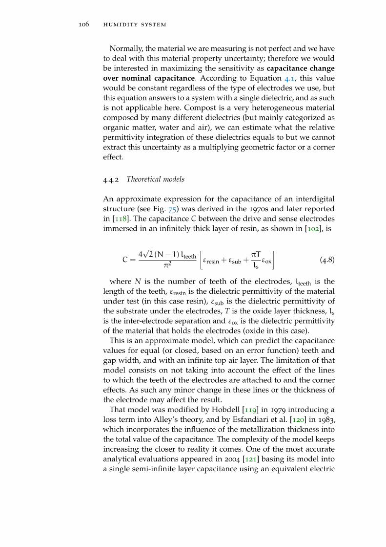
106 humidity system
Normally, the material we are measuring is not perfect and we haveto deal with this material property uncertainty; therefore we wouldbe interested in maximizing the sensitivity as capacitance changeover nominal capacitance. According to Equation 4.1, this valuewould be constant regardless of the type of electrodes we use, butthis equation answers to a system with a single dielectric, and as suchis not applicable here. Compost is a very heterogeneous materialcomposed by many different dielectrics (but mainly categorized asorganic matter, water and air), we can estimate what the relativepermittivity integration of these dielectrics equals to but we cannotextract this uncertainty as a multiplying geometric factor or a cornereffect.
4.4.2 Theoretical models
An approximate expression for the capacitance of an interdigitalstructure (see Fig. 75) was derived in the 1970s and later reportedin [118]. The capacitance C between the drive and sense electrodesimmersed in an infinitely thick layer of resin, as shown in [102], is
C =4√2 (N− 1) lteeth
π2
[εresin + εsub +
πT
lsεox
](4.8)
where N is the number of teeth of the electrodes, lteeth is thelength of the teeth, εresin is the dielectric permittivity of the materialunder test (in this case resin), εsub is the dielectric permittivity ofthe substrate under the electrodes, T is the oxide layer thickness, lsis the inter-electrode separation and εox is the dielectric permittivityof the material that holds the electrodes (oxide in this case).
This is an approximate model, which can predict the capacitancevalues for equal (or closed, based on an error function) teeth andgap width, and with an infinite top air layer. The limitation of thatmodel consists on not taking into account the effect of the linesto which the teeth of the electrodes are attached to and the cornereffects. As such any minor change in these lines or the thickness ofthe electrode may affect the result.
That model was modified by Hobdell [119] in 1979 introducing aloss term into Alley’s theory, and by Esfandiari et al. [120] in 1983,which incorporates the influence of the metallization thickness intothe total value of the capacitance. The complexity of the model keepsincreasing the closer to reality it comes. One of the most accurateanalytical evaluations appeared in 2004 [121] basing its model intoa single semi-infinite layer capacitance using an equivalent electric
4.4 single-layer coplanar capacitive electrodes 107
Figure 75: 3D Interdigital electrodes
circuit. For symmetry reasons, the capacitance is evaluated as a func-tion of two types of capacitance: (1) CI—being half the capacitanceof one interior teeth relative to the ground potential and (2) CE—thecapacitance of one outer teeth relative to the ground plane next to it.
C = (N− 3)CI
2+ 2
CICE
CI +CE, N > 3 (4.9)
where N is the number of teeth. The calculation of CE and CIincludes complex calculations as complete elliptic integrals of firstkind, and does not take into account the influence of corner effects.
The processing of such complex theoretical models require heavycomputational work that would imply spending great effort and timein something that can be easily done using simulation tools. Also,taking into account the inaccuracy of approximated calculations wedecided simulating the different electrode configurations in order tohave the highest accuracy with the minimum complexity. Moreover,whilst there are different theoretical models for each shape, thesimulation process is the same.
In the case of concentric capacitive electrodes, the capacitance CTbetween the two electrodes, can be calculated through [105]
CT =Qouter
Vinner
∣∣∣∣Vouter=0
(4.10)
where Qouter is the total charge on the outer electrode, while Vinnerand Vouter respectively represent the voltage on the inner and outer
108 humidity system
electrodes. The total charge, on both inner and outer electrodes, canbe found integrating over the electrode surfaces with the surfacecharge distribution σ (ρ ′). In order to calculate the surface chargedistribution, Green’s functions [122] for the method of moments(MoM) [123] are used. We have to take into account that the methodof moments is used in simulation tools, and hence we see thatfor complex theoretical models in the case of concentric capacitiveelectrodes the option is also simulating.
Considering all previous models we will work with simulations tofulfill our objective of finding the design optimization for interdigitaland concentric electrodes.
4.4.3 Simulation
All the simulations were realized with COMSOL Multiphysics v4.2aon a computer running Windows 7 Enterprise with a processor IntelCore i7 CPU 860 @ 2.80 GHz, a RAM memory of 16 GBytes and a 64
bit OS.In all the cases, a 2 m environment sphere was created as compost
implying that the electrodes are surrounded by a very big compostmass (relative permittivity changed from 10 to 15, in other words,from a lower humidity to a higher) with a zero charge electrostaticstate, along with a pair of copper coplanar electrodes (with one ofthem as 3 V electric potential and the other as ground) in the centerand a copper active shield 1 mm under them (with 3 V of electricpotential), that focuses the area affected by the electrodes to the front.The electrodes and the active shield were separated by a 1 mm layerof resin (relative permittivity of 3.1 [63]), as in the typical printedcircuit plaques, with a charge conservation electrostatic state.
The area of the concentric and the interdigital electrodes is thesame in all the cases; as such, the concentric electrodes are a circularplaque of radius 3 cm and the interdigital electrodes are a squaredplaque of side 5.3 cm. The different configurations have been thoughtwithin these dimensions and the limit values for each dimensionwere tested.
The simulations had an extra fine mesh and the electrode capac-itance (C) was evaluated as an integration of the active electrodesurface charge density (σ) divided by the applied voltage differenceacross the electrodes (∆V)[124], similarly to what we saw in equation4.10
C =
∫σ
∆VdA (4.11)
4.4 single-layer coplanar capacitive electrodes 109
The capacitance of electrodes could also be calculated as the inte-gration of the ground electrode surface charge density divided bythe voltage or as the global evaluation of the total stored electricenergy (We) divided by the voltage difference across the electrodes∆V[125]
C =2 ·We
∆V2(4.12)
The problem of the integration of the ground electrode and theglobal evaluation is that they include the electromagnetic fieldsgoing from the active shield to ground and therefore the resultwould not purely be the effect of the sensing electrode to the groundelectrode.
From the capacitance value, there will be three variables analyzed:the nominal capacitance (C1 and C2, that are the capacitance valuesof the electrode for a relative permittivity of 10 and 15 respectively),the capacitance change and the capacitance change over the nominalcapacitance. The nominal capacitance value is interesting for appli-cations needing a minimum value of capacitance. The capacitancechange (4C) is interesting for applications in which the predomi-nant disturbance is the noise of the system, which does not change infunction of the permittivity and is defined as the difference betweenC1 to C2. And the capacitance change over the nominal capacitance(4C/C1) is interesting for applications in which the predominantdisturbance is the inaccuracy due to the heterogeneity of the mate-rial.
Concentric electrodes
The concentric electrodes (Fig. 76) consisted of an active circularelectrode of radius ra and thickness 1 mm, surrounded by a groundring electrode of outer radius of 3 cm, inner radius rg,i and thickness1 mm. The resin layer and the active shield were 6 cm radius circleswith 1 mm thickness.
The simulations were realized in order to see the performanceof the electrodes when varying the separation between electrodesor the size of one electrode respect to the others. As follows, thenominal capacitance of the electrodes, their capacitance change andtheir capacitance change over the nominal capacitance are calculatedin function of the separation between electrodes and the size of theactive electrode radius.
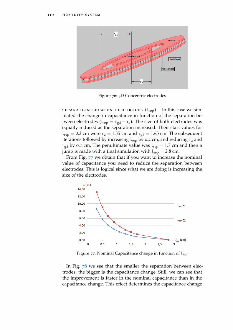
110 humidity system
Figure 76: 3D Concentric electrodes
separation between electrodes (lsep ) In this case we sim-ulated the change in capacitance in function of the separation be-tween electrodes (lsep = rg,i − ra). The size of both electrodes wasequally reduced as the separation increased. Their start values forlsep = 0.3 cm were ra = 1.35 cm and rg,i = 1.65 cm. The subsequentiterations followed by increasing lsep by 0.2 cm, and reducing ra andrg,i by 0.1 cm. The penultimate value was lsep = 1.7 cm and then ajump is made with a final simulation with lsep = 2.8 cm.
From Fig. 77 we obtain that if you want to increase the nominalvalue of capacitance you need to reduce the separation betweenelectrodes. This is logical since what we are doing is increasing thesize of the electrodes.
Figure 77: Nominal Capacitance change in function of lsep
In Fig. 78 we see that the smaller the separation between elec-trodes, the bigger is the capacitance change. Still, we can see thatthe improvement is faster in the nominal capacitance than in thecapacitance change. This effect determines the capacitance change
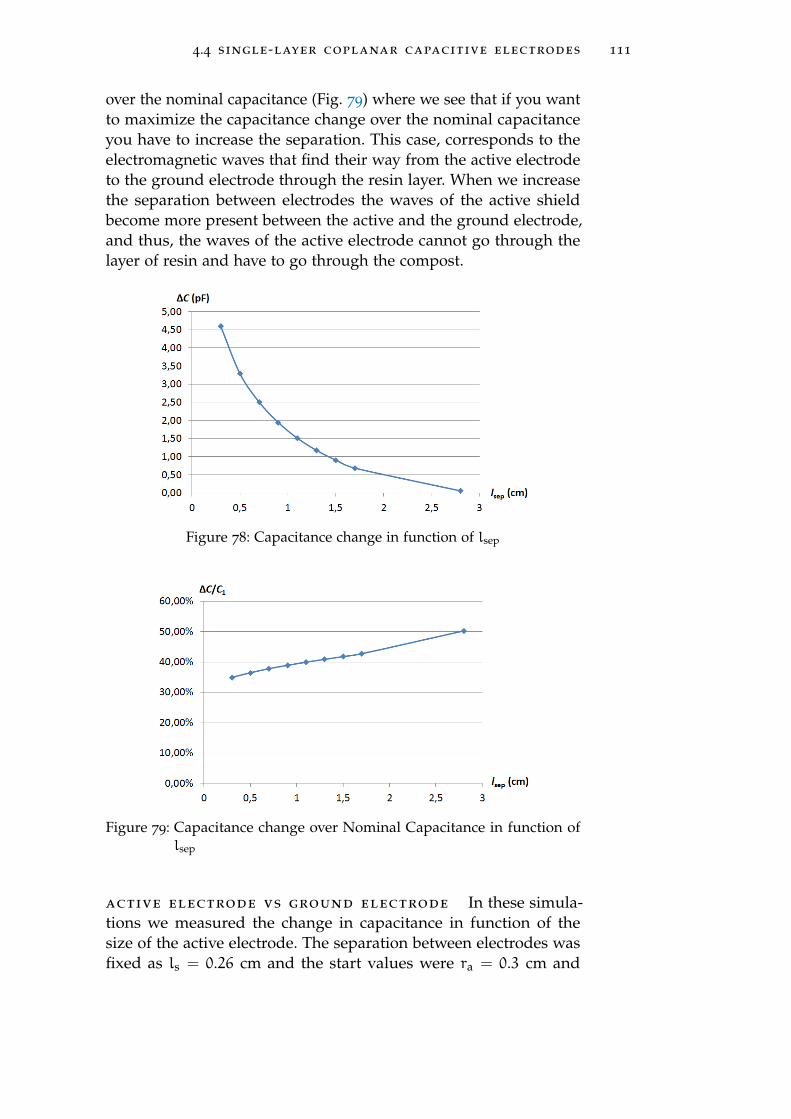
4.4 single-layer coplanar capacitive electrodes 111
over the nominal capacitance (Fig. 79) where we see that if you wantto maximize the capacitance change over the nominal capacitanceyou have to increase the separation. This case, corresponds to theelectromagnetic waves that find their way from the active electrodeto the ground electrode through the resin layer. When we increasethe separation between electrodes the waves of the active shieldbecome more present between the active and the ground electrode,and thus, the waves of the active electrode cannot go through thelayer of resin and have to go through the compost.
Figure 78: Capacitance change in function of lsep
Figure 79: Capacitance change over Nominal Capacitance in function oflsep
active electrode vs ground electrode In these simula-tions we measured the change in capacitance in function of thesize of the active electrode. The separation between electrodes wasfixed as ls = 0.26 cm and the start values were ra = 0.3 cm and
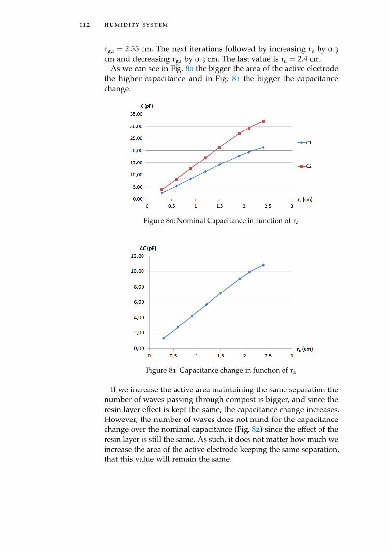
112 humidity system
rg,i = 2.55 cm. The next iterations followed by increasing ra by 0.3cm and decreasing rg,i by 0.3 cm. The last value is ra = 2.4 cm.
As we can see in Fig. 80 the bigger the area of the active electrodethe higher capacitance and in Fig. 81 the bigger the capacitancechange.
Figure 80: Nominal Capacitance in function of ra
Figure 81: Capacitance change in function of ra
If we increase the active area maintaining the same separation thenumber of waves passing through compost is bigger, and since theresin layer effect is kept the same, the capacitance change increases.However, the number of waves does not mind for the capacitancechange over the nominal capacitance (Fig. 82) since the effect of theresin layer is still the same. As such, it does not matter how much weincrease the area of the active electrode keeping the same separation,that this value will remain the same.
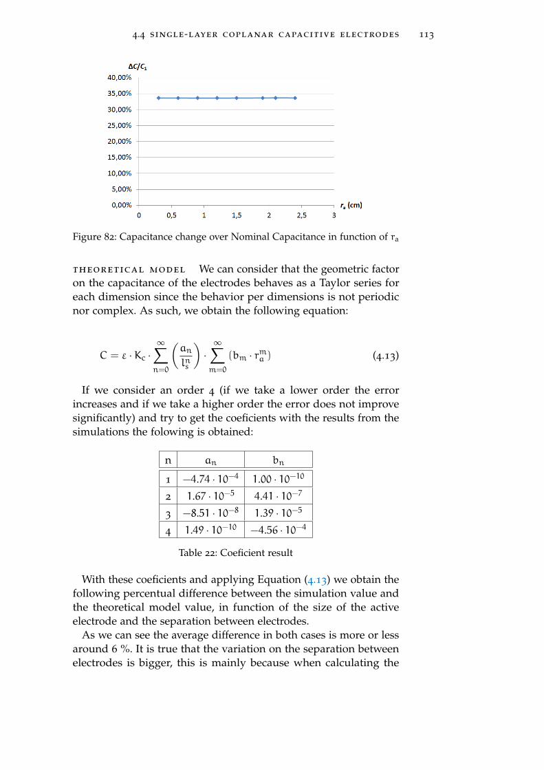
4.4 single-layer coplanar capacitive electrodes 113
Figure 82: Capacitance change over Nominal Capacitance in function of ra
theoretical model We can consider that the geometric factoron the capacitance of the electrodes behaves as a Taylor series foreach dimension since the behavior per dimensions is not periodicnor complex. As such, we obtain the following equation:
C = ε ·Kc ·∞∑n=0
(an
lns
)·
∞∑m=0
(bm · rma ) (4.13)
If we consider an order 4 (if we take a lower order the errorincreases and if we take a higher order the error does not improvesignificantly) and try to get the coeficients with the results from thesimulations the folowing is obtained:
n an bn
1 −4.74 · 10−4 1.00 · 10−10
2 1.67 · 10−5 4.41 · 10−7
3 −8.51 · 10−8 1.39 · 10−5
4 1.49 · 10−10 −4.56 · 10−4
Table 22: Coeficient result
With these coeficients and applying Equation (4.13) we obtain thefollowing percentual difference between the simulation value andthe theoretical model value, in function of the size of the activeelectrode and the separation between electrodes.
As we can see the average difference in both cases is more or lessaround 6 %. It is true that the variation on the separation betweenelectrodes is bigger, this is mainly because when calculating the
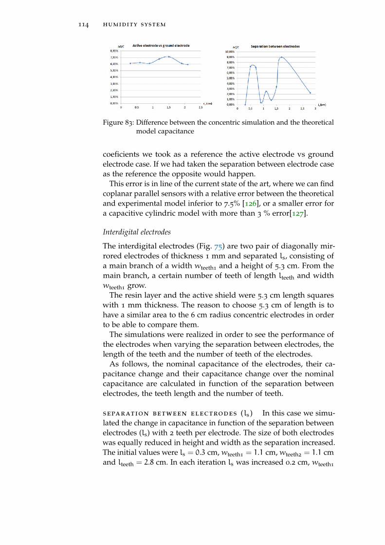
114 humidity system
Figure 83: Difference between the concentric simulation and the theoreticalmodel capacitance
coeficients we took as a reference the active electrode vs groundelectrode case. If we had taken the separation between electrode caseas the reference the opposite would happen.
This error is in line of the current state of the art, where we can findcoplanar parallel sensors with a relative error between the theoreticaland experimental model inferior to 7.5% [126], or a smaller error fora capacitive cylindric model with more than 3 % error[127].
Interdigital electrodes
The interdigital electrodes (Fig. 75) are two pair of diagonally mir-rored electrodes of thickness 1 mm and separated ls, consisting ofa main branch of a width wteeth1
and a height of 5.3 cm. From themain branch, a certain number of teeth of length lteeth and widthwteeth1
grow.The resin layer and the active shield were 5.3 cm length squares
with 1 mm thickness. The reason to choose 5.3 cm of length is tohave a similar area to the 6 cm radius concentric electrodes in orderto be able to compare them.
The simulations were realized in order to see the performance ofthe electrodes when varying the separation between electrodes, thelength of the teeth and the number of teeth of the electrodes.
As follows, the nominal capacitance of the electrodes, their ca-pacitance change and their capacitance change over the nominalcapacitance are calculated in function of the separation betweenelectrodes, the teeth length and the number of teeth.
separation between electrodes (ls ) In this case we simu-lated the change in capacitance in function of the separation betweenelectrodes (ls) with 2 teeth per electrode. The size of both electrodeswas equally reduced in height and width as the separation increased.The initial values were ls = 0.3 cm,wteeth1
= 1.1 cm,wteeth2= 1.1 cm
and lteeth = 2.8 cm. In each iteration ls was increased 0.2 cm, wteeth1
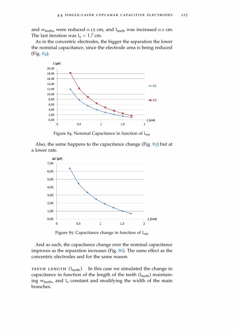
4.4 single-layer coplanar capacitive electrodes 115
and wteeth2were reduced 0.15 cm, and lteeth was increased 0.1 cm.
The last iteration was ls = 1.7 cm.As in the concentric electrodes, the bigger the separation the lower
the nominal capacitance, since the electrode area is being reduced(Fig. 84).
Figure 84: Nominal Capacitance in function of lsep
Also, the same happens to the capacitance change (Fig. 85) but ata lower rate.
Figure 85: Capacitance change in function of lsep
And as such, the capacitance change over the nominal capacitanceimproves as the separation increases (Fig. 86). The same effect as theconcentric electrodes and for the same reason.
teeth length (lteeth ) In this case we simulated the change incapacitance in function of the length of the teeth (lteeth) maintain-ing wteeth1
and ls constant and modifying the width of the mainbranches.
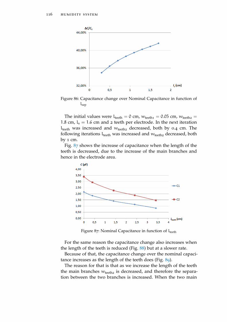
116 humidity system
Figure 86: Capacitance change over Nominal Capacitance in function oflsep
The initial values were lteeth = 0 cm, wteeth1= 0.05 cm, wteeth2
=
1.8 cm, ls = 1.6 cm and 2 teeth per electrode. In the next iterationlteeth was increased and wteeth2
decreased, both by 0.4 cm. Thefollowing iterations lteeth was increased and wteeth2
decreased, bothby 1 cm.
Fig. 87 shows the increase of capacitance when the length of theteeth is decreased, due to the increase of the main branches andhence in the electrode area.
Figure 87: Nominal Capacitance in function of lteeth
For the same reason the capacitance change also increases whenthe length of the teeth is reduced (Fig. 88) but at a slower rate.
Because of that, the capacitance change over the nominal capaci-tance increases as the length of the teeth does (Fig. 89).
The reason for that is that as we increase the length of the teeththe main branches wteeth2
is decreased, and therefore the separa-tion between the two branches is increased. When the two main
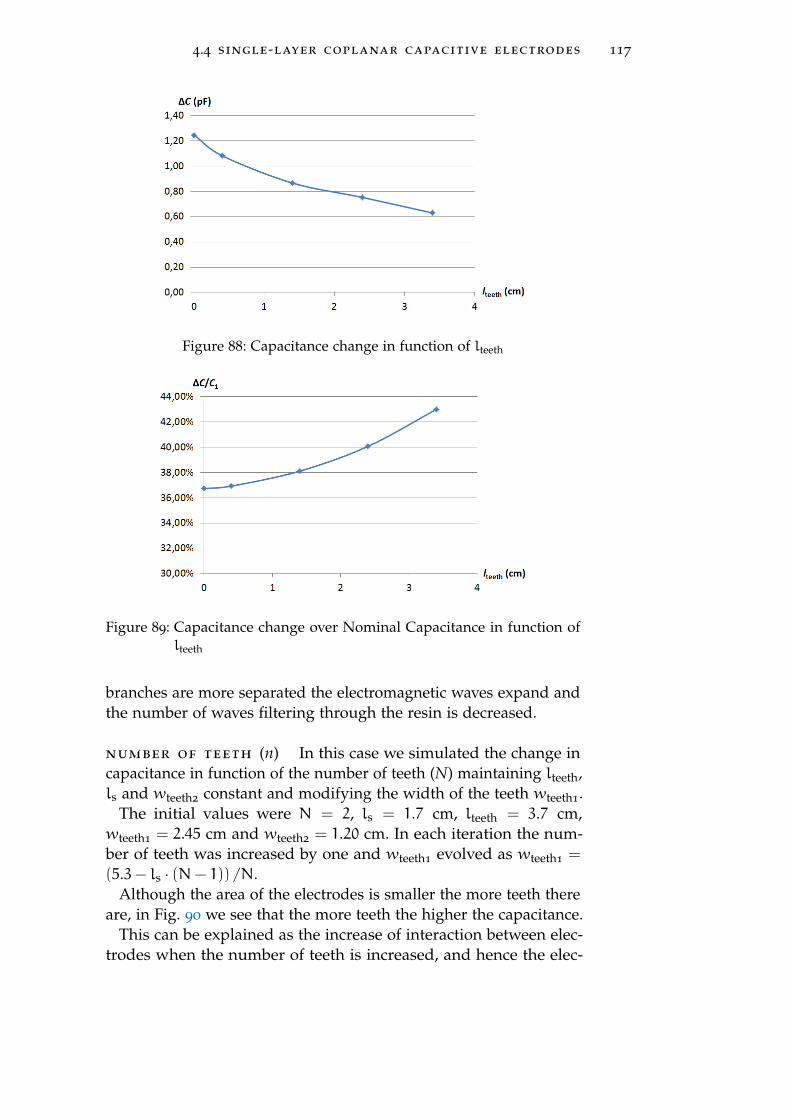
4.4 single-layer coplanar capacitive electrodes 117
Figure 88: Capacitance change in function of lteeth
Figure 89: Capacitance change over Nominal Capacitance in function oflteeth
branches are more separated the electromagnetic waves expand andthe number of waves filtering through the resin is decreased.
number of teeth (n) In this case we simulated the change incapacitance in function of the number of teeth (N) maintaining lteeth,ls and wteeth2
constant and modifying the width of the teeth wteeth1.
The initial values were N = 2, ls = 1.7 cm, lteeth = 3.7 cm,wteeth1
= 2.45 cm and wteeth2= 1.20 cm. In each iteration the num-
ber of teeth was increased by one and wteeth1evolved as wteeth1
=
(5.3− ls · (N− 1)) /N.Although the area of the electrodes is smaller the more teeth there
are, in Fig. 90 we see that the more teeth the higher the capacitance.This can be explained as the increase of interaction between elec-
trodes when the number of teeth is increased, and hence the elec-
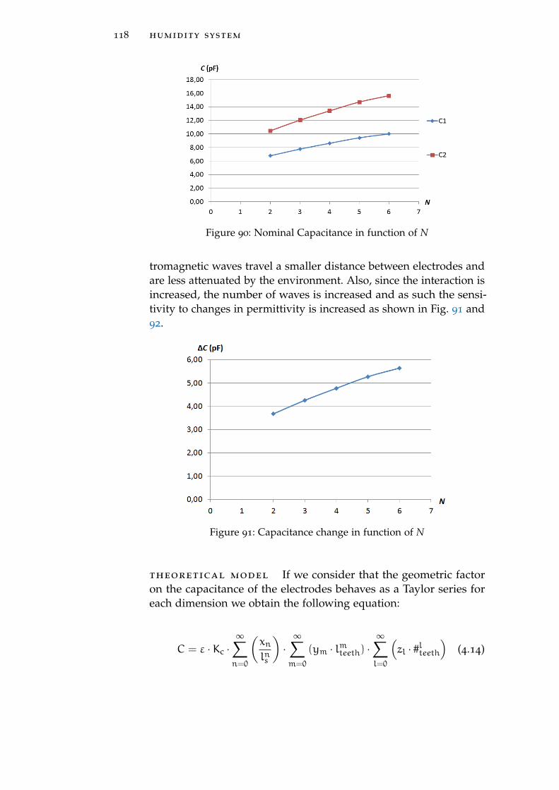
118 humidity system
Figure 90: Nominal Capacitance in function of N
tromagnetic waves travel a smaller distance between electrodes andare less attenuated by the environment. Also, since the interaction isincreased, the number of waves is increased and as such the sensi-tivity to changes in permittivity is increased as shown in Fig. 91 and92.
Figure 91: Capacitance change in function of N
theoretical model If we consider that the geometric factoron the capacitance of the electrodes behaves as a Taylor series foreach dimension we obtain the following equation:
C = ε ·Kc ·∞∑n=0
(xn
lns
)·
∞∑m=0
(ym · lmteeth) ·∞∑l=0
(zl · #lteeth
)(4.14)
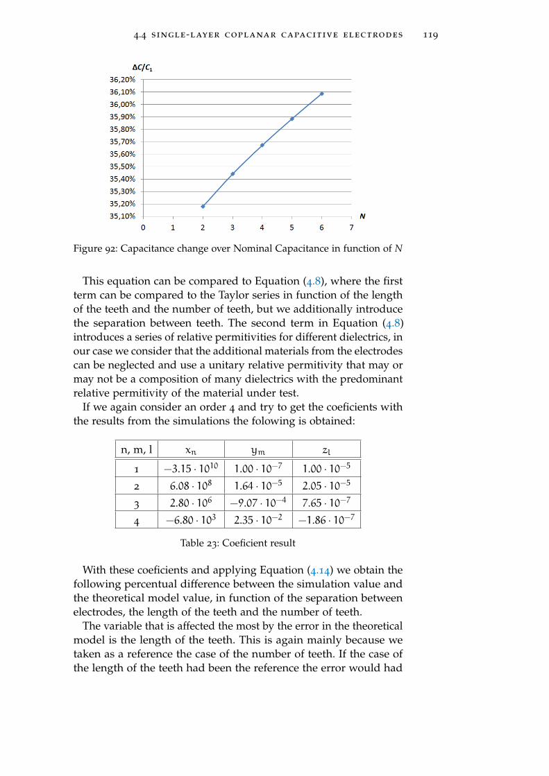
4.4 single-layer coplanar capacitive electrodes 119
Figure 92: Capacitance change over Nominal Capacitance in function of N
This equation can be compared to Equation (4.8), where the firstterm can be compared to the Taylor series in function of the lengthof the teeth and the number of teeth, but we additionally introducethe separation between teeth. The second term in Equation (4.8)introduces a series of relative permitivities for different dielectrics, inour case we consider that the additional materials from the electrodescan be neglected and use a unitary relative permitivity that may ormay not be a composition of many dielectrics with the predominantrelative permitivity of the material under test.
If we again consider an order 4 and try to get the coeficients withthe results from the simulations the folowing is obtained:
n, m, l xn ym zl
1 −3.15 · 1010 1.00 · 10−7 1.00 · 10−5
2 6.08 · 108 1.64 · 10−5 2.05 · 10−5
3 2.80 · 106 −9.07 · 10−4 7.65 · 10−7
4 −6.80 · 103 2.35 · 10−2 −1.86 · 10−7
Table 23: Coeficient result
With these coeficients and applying Equation (4.14) we obtain thefollowing percentual difference between the simulation value andthe theoretical model value, in function of the separation betweenelectrodes, the length of the teeth and the number of teeth.
The variable that is affected the most by the error in the theoreticalmodel is the length of the teeth. This is again mainly because wetaken as a reference the case of the number of teeth. If the case ofthe length of the teeth had been the reference the error would had
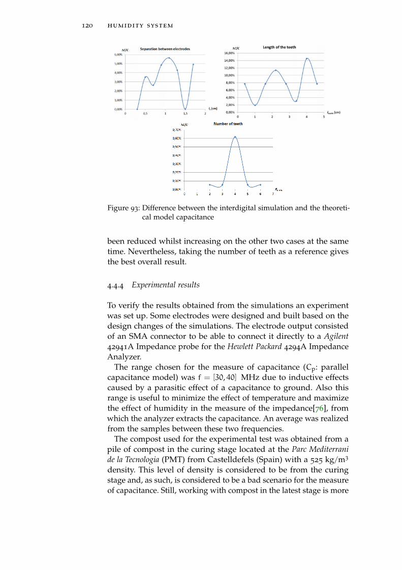
120 humidity system
Figure 93: Difference between the interdigital simulation and the theoreti-cal model capacitance
been reduced whilst increasing on the other two cases at the sametime. Nevertheless, taking the number of teeth as a reference givesthe best overall result.
4.4.4 Experimental results
To verify the results obtained from the simulations an experimentwas set up. Some electrodes were designed and built based on thedesign changes of the simulations. The electrode output consistedof an SMA connector to be able to connect it directly to a Agilent42941A Impedance probe for the Hewlett Packard 4294A ImpedanceAnalyzer.
The range chosen for the measure of capacitance (Cp: parallelcapacitance model) was f = [30, 40] MHz due to inductive effectscaused by a parasitic effect of a capacitance to ground. Also thisrange is useful to minimize the effect of temperature and maximizethe effect of humidity in the measure of the impedance[76], fromwhich the analyzer extracts the capacitance. An average was realizedfrom the samples between these two frequencies.
The compost used for the experimental test was obtained from apile of compost in the curing stage located at the Parc Mediterranide la Tecnologia (PMT) from Castelldefels (Spain) with a 525 kg/m3
density. This level of density is considered to be from the curingstage and, as such, is considered to be a bad scenario for the measureof capacitance. Still, working with compost in the latest stage is more
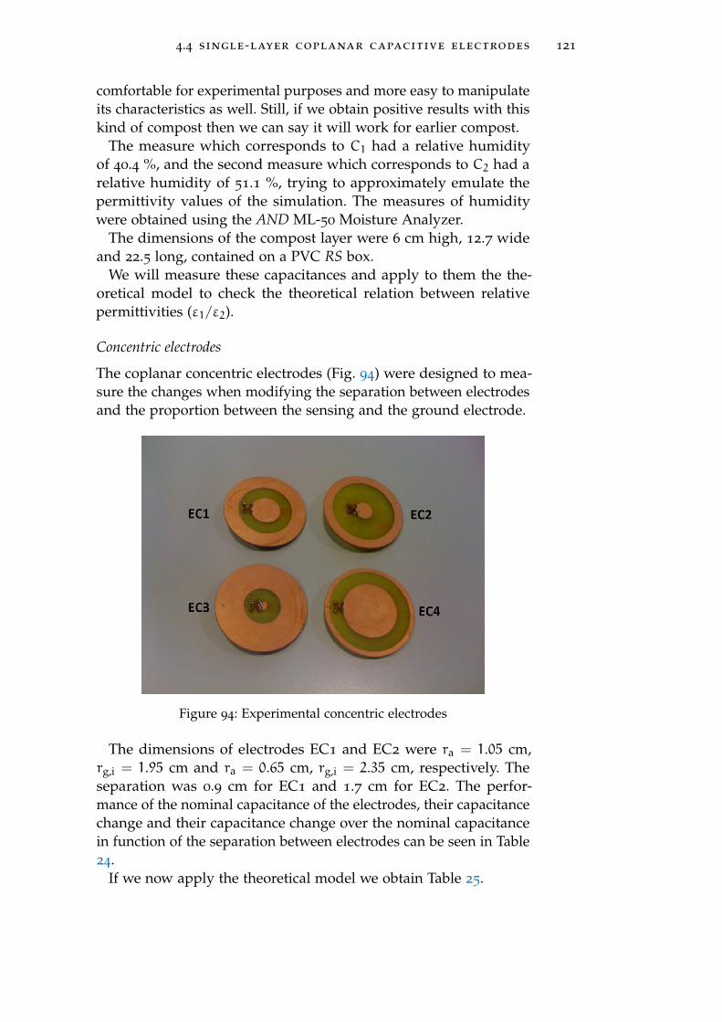
4.4 single-layer coplanar capacitive electrodes 121
comfortable for experimental purposes and more easy to manipulateits characteristics as well. Still, if we obtain positive results with thiskind of compost then we can say it will work for earlier compost.
The measure which corresponds to C1 had a relative humidityof 40.4 %, and the second measure which corresponds to C2 had arelative humidity of 51.1 %, trying to approximately emulate thepermittivity values of the simulation. The measures of humiditywere obtained using the AND ML-50 Moisture Analyzer.
The dimensions of the compost layer were 6 cm high, 12.7 wideand 22.5 long, contained on a PVC RS box.
We will measure these capacitances and apply to them the the-oretical model to check the theoretical relation between relativepermittivities (ε1/ε2).
Concentric electrodes
The coplanar concentric electrodes (Fig. 94) were designed to mea-sure the changes when modifying the separation between electrodesand the proportion between the sensing and the ground electrode.
Figure 94: Experimental concentric electrodes
The dimensions of electrodes EC1 and EC2 were ra = 1.05 cm,rg,i = 1.95 cm and ra = 0.65 cm, rg,i = 2.35 cm, respectively. Theseparation was 0.9 cm for EC1 and 1.7 cm for EC2. The perfor-mance of the nominal capacitance of the electrodes, their capacitancechange and their capacitance change over the nominal capacitancein function of the separation between electrodes can be seen in Table24.
If we now apply the theoretical model we obtain Table 25.
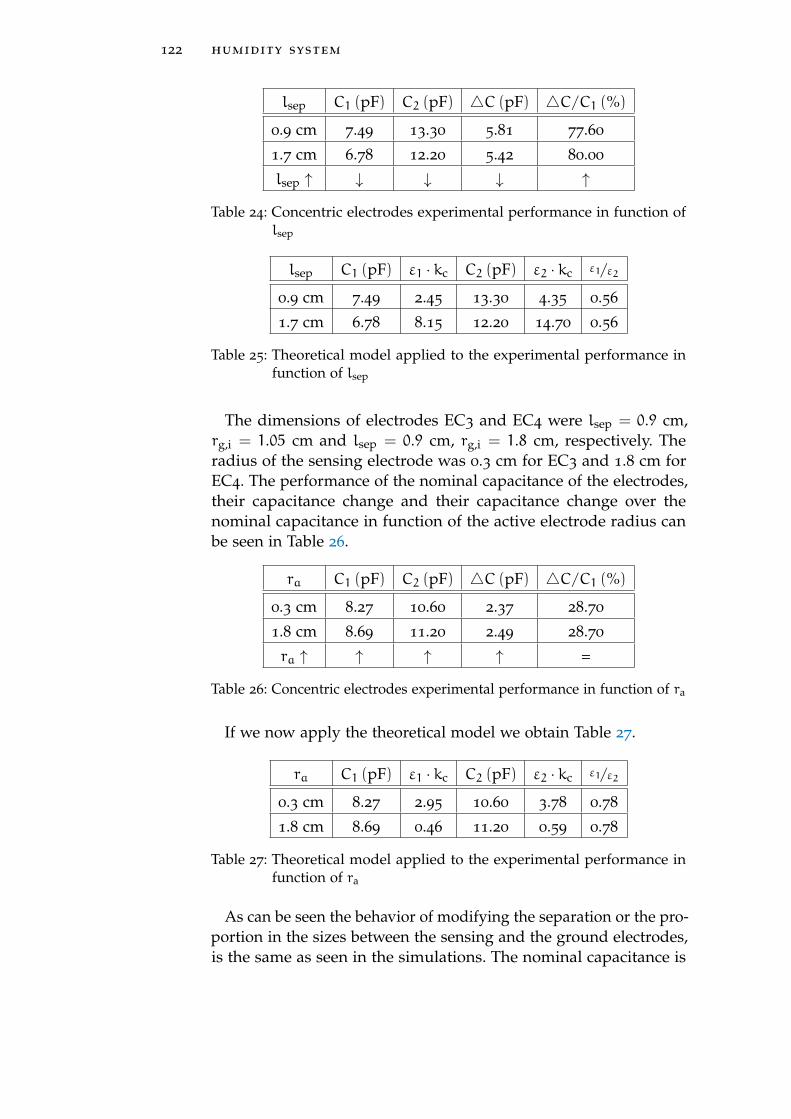
122 humidity system
lsep C1 (pF) C2 (pF) 4C (pF) 4C/C1 (%)
0.9 cm 7.49 13.30 5.81 77.60
1.7 cm 6.78 12.20 5.42 80.00
lsep ↑ ↓ ↓ ↓ ↑
Table 24: Concentric electrodes experimental performance in function oflsep
lsep C1 (pF) ε1 · kc C2 (pF) ε2 · kc ε1/ε2
0.9 cm 7.49 2.45 13.30 4.35 0.56
1.7 cm 6.78 8.15 12.20 14.70 0.56
Table 25: Theoretical model applied to the experimental performance infunction of lsep
The dimensions of electrodes EC3 and EC4 were lsep = 0.9 cm,rg,i = 1.05 cm and lsep = 0.9 cm, rg,i = 1.8 cm, respectively. Theradius of the sensing electrode was 0.3 cm for EC3 and 1.8 cm forEC4. The performance of the nominal capacitance of the electrodes,their capacitance change and their capacitance change over thenominal capacitance in function of the active electrode radius canbe seen in Table 26.
ra C1 (pF) C2 (pF) 4C (pF) 4C/C1 (%)
0.3 cm 8.27 10.60 2.37 28.70
1.8 cm 8.69 11.20 2.49 28.70
ra ↑ ↑ ↑ ↑ =
Table 26: Concentric electrodes experimental performance in function of ra
If we now apply the theoretical model we obtain Table 27.
ra C1 (pF) ε1 · kc C2 (pF) ε2 · kc ε1/ε2
0.3 cm 8.27 2.95 10.60 3.78 0.78
1.8 cm 8.69 0.46 11.20 0.59 0.78
Table 27: Theoretical model applied to the experimental performance infunction of ra
As can be seen the behavior of modifying the separation or the pro-portion in the sizes between the sensing and the ground electrodes,is the same as seen in the simulations. The nominal capacitance is
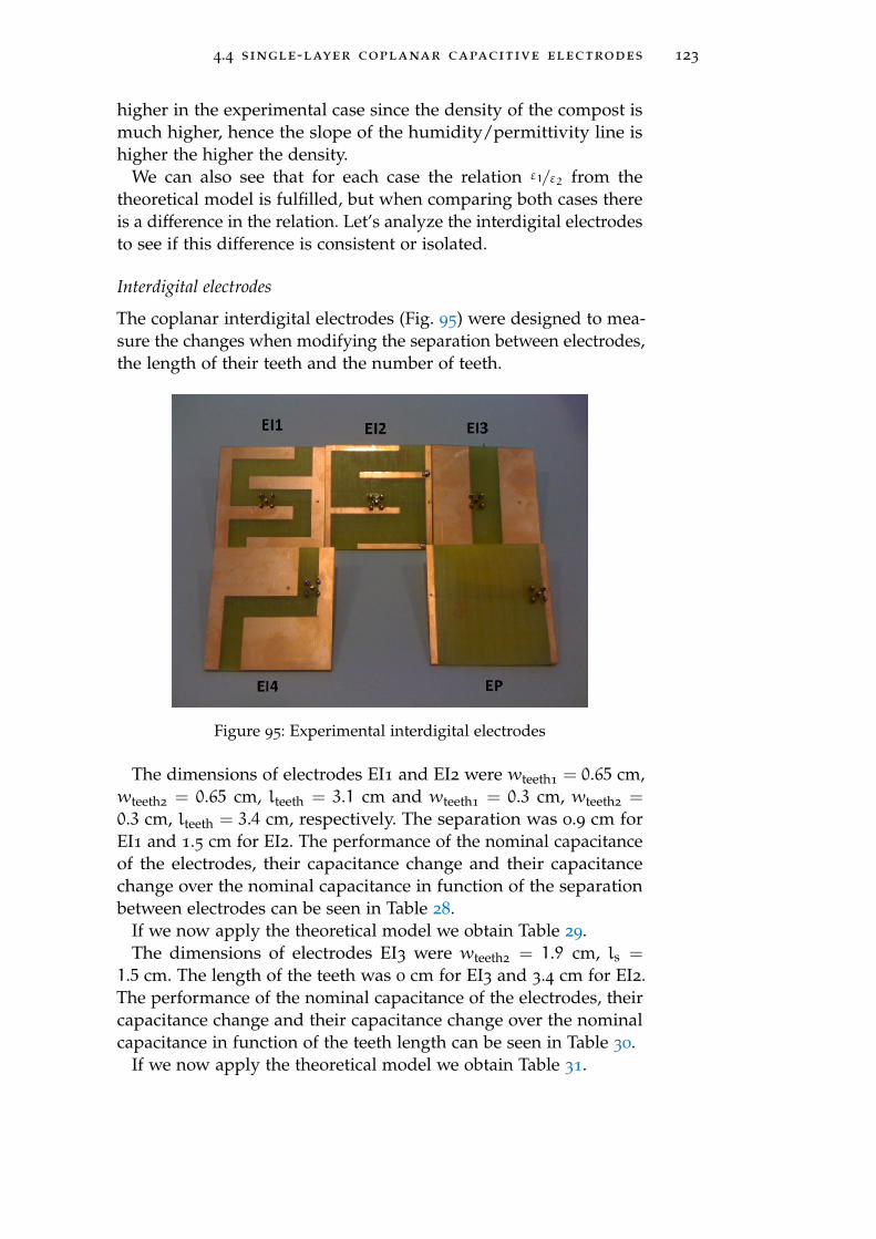
4.4 single-layer coplanar capacitive electrodes 123
higher in the experimental case since the density of the compost ismuch higher, hence the slope of the humidity/permittivity line ishigher the higher the density.
We can also see that for each case the relation ε1/ε2 from thetheoretical model is fulfilled, but when comparing both cases thereis a difference in the relation. Let’s analyze the interdigital electrodesto see if this difference is consistent or isolated.
Interdigital electrodes
The coplanar interdigital electrodes (Fig. 95) were designed to mea-sure the changes when modifying the separation between electrodes,the length of their teeth and the number of teeth.
Figure 95: Experimental interdigital electrodes
The dimensions of electrodes EI1 and EI2 were wteeth1= 0.65 cm,
wteeth2= 0.65 cm, lteeth = 3.1 cm and wteeth1
= 0.3 cm, wteeth2=
0.3 cm, lteeth = 3.4 cm, respectively. The separation was 0.9 cm forEI1 and 1.5 cm for EI2. The performance of the nominal capacitanceof the electrodes, their capacitance change and their capacitancechange over the nominal capacitance in function of the separationbetween electrodes can be seen in Table 28.
If we now apply the theoretical model we obtain Table 29.The dimensions of electrodes EI3 were wteeth2
= 1.9 cm, ls =
1.5 cm. The length of the teeth was 0 cm for EI3 and 3.4 cm for EI2.The performance of the nominal capacitance of the electrodes, theircapacitance change and their capacitance change over the nominalcapacitance in function of the teeth length can be seen in Table 30.
If we now apply the theoretical model we obtain Table 31.
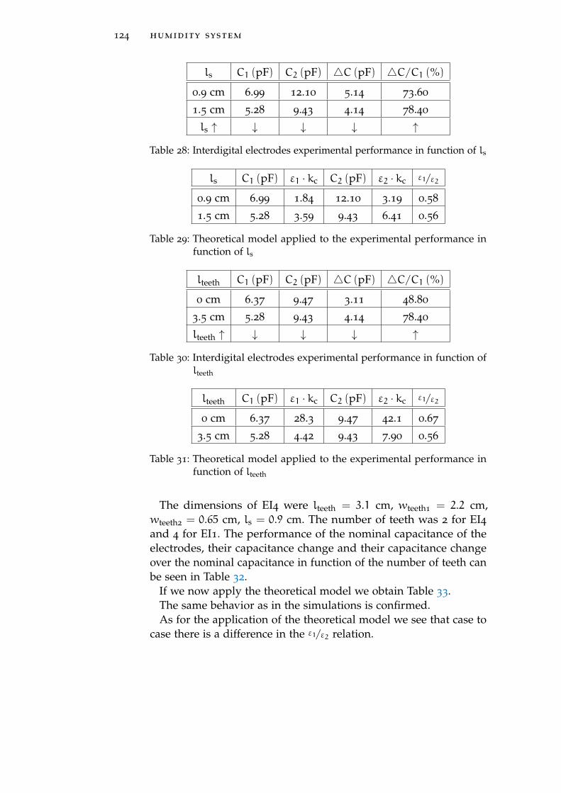
124 humidity system
ls C1 (pF) C2 (pF) 4C (pF) 4C/C1 (%)
0.9 cm 6.99 12.10 5.14 73.60
1.5 cm 5.28 9.43 4.14 78.40
ls ↑ ↓ ↓ ↓ ↑
Table 28: Interdigital electrodes experimental performance in function of ls
ls C1 (pF) ε1 · kc C2 (pF) ε2 · kc ε1/ε2
0.9 cm 6.99 1.84 12.10 3.19 0.58
1.5 cm 5.28 3.59 9.43 6.41 0.56
Table 29: Theoretical model applied to the experimental performance infunction of ls
lteeth C1 (pF) C2 (pF) 4C (pF) 4C/C1 (%)
0 cm 6.37 9.47 3.11 48.80
3.5 cm 5.28 9.43 4.14 78.40
lteeth ↑ ↓ ↓ ↓ ↑
Table 30: Interdigital electrodes experimental performance in function oflteeth
lteeth C1 (pF) ε1 · kc C2 (pF) ε2 · kc ε1/ε2
0 cm 6.37 28.3 9.47 42.1 0.67
3.5 cm 5.28 4.42 9.43 7.90 0.56
Table 31: Theoretical model applied to the experimental performance infunction of lteeth
The dimensions of EI4 were lteeth = 3.1 cm, wteeth1= 2.2 cm,
wteeth2= 0.65 cm, ls = 0.9 cm. The number of teeth was 2 for EI4
and 4 for EI1. The performance of the nominal capacitance of theelectrodes, their capacitance change and their capacitance changeover the nominal capacitance in function of the number of teeth canbe seen in Table 32.
If we now apply the theoretical model we obtain Table 33.The same behavior as in the simulations is confirmed.As for the application of the theoretical model we see that case to
case there is a difference in the ε1/ε2 relation.
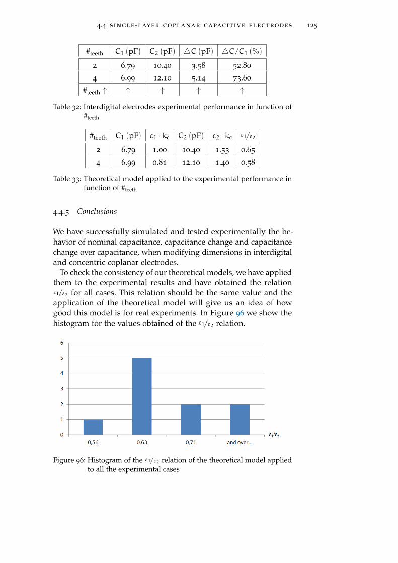
4.4 single-layer coplanar capacitive electrodes 125
#teeth C1 (pF) C2 (pF) 4C (pF) 4C/C1 (%)
2 6.79 10.40 3.58 52.80
4 6.99 12.10 5.14 73.60
#teeth ↑ ↑ ↑ ↑ ↑
Table 32: Interdigital electrodes experimental performance in function of#teeth
#teeth C1 (pF) ε1 · kc C2 (pF) ε2 · kc ε1/ε2
2 6.79 1.00 10.40 1.53 0.65
4 6.99 0.81 12.10 1.40 0.58
Table 33: Theoretical model applied to the experimental performance infunction of #teeth
4.4.5 Conclusions
We have successfully simulated and tested experimentally the be-havior of nominal capacitance, capacitance change and capacitancechange over capacitance, when modifying dimensions in interdigitaland concentric coplanar electrodes.
To check the consistency of our theoretical models, we have appliedthem to the experimental results and have obtained the relationε1/ε2 for all cases. This relation should be the same value and theapplication of the theoretical model will give us an idea of howgood this model is for real experiments. In Figure 96 we show thehistogram for the values obtained of the ε1/ε2 relation.
Figure 96: Histogram of the ε1/ε2 relation of the theoretical model appliedto all the experimental cases
126 humidity system
The average of the values is around 0.63 and the standard deviation0.08. If we calculate the standard error of the mean we obtain 2.82 %which gives us a good feeling of the consistency of the theoreticalmodel when using it on our theoretical models for concentric andinterdigital electrodes.
On the other hand, the following recommendations for the designof electrodes where obtained from the behavior of the electrodes:
If we were interested in an application that needs a minimumvalue of capacitance and/or an application in which the predom-inant disturbance is the noise of the system (is not affected bythe uncertainty in the material composition), we can use concentricelectrodes to have the biggest nominal capacitance (C) and/or thebiggest sensitivity (4C) respectively. For both cases we need todecrease the separation between electrodes and to make the sensingelectrode much bigger than the ground electrode.
If we were interested in avoiding corner effects, regardless of thenominal capacitance (C) and the sensitivity (4C), we should useconcentric electrodes maximizing the relative sensitivity (4C/C1),increasing the separation as much as possible.
Since we are interested in an application in which the predom-inant disturbance is the inaccuracy due to the heterogeneity ofthe material, we will use interdigital electrodes to have the biggestrelative sensitivity (4C/C1). In that case we need to increase the sep-aration between electrodes, the length of the teeth and the numberof teeth.
If we were able to choose the size of the electrodes, then weshould have chosen to make them as big as possible, not only toincrease their nominal capacitance (C), but also their sensitivity(4C).
Also we could have played and mix characteristics of electrodes bydesigning hybrids electrodes, e.g. a concentric interdigital electrodeto avoid corner effects and to increase the relative sensitivity asmuch as possible.
4.5 multilayer coplanar capacitive electrodes
Dielectric materials play an extensive role in both industrial appli-cations and scientific research areas. Due to the need of electriccomponent miniaturization in modern integrated circuit industry,there are palpable needs for dielectric measurements of low-lossthin materials [105].
One important and practical field of material dielectric propertycharacterization is dielectrometry, which derives the complex permit-
4.5 multilayer coplanar capacitive electrodes 127
tivity of a test-piece from the measured sensor capacitance. Sensorsbased in coplanar capacitive electrodes are widespread among themost commonly used. Recent advances in such fields as nonde-structive testing (NDT), microelectromechanical systems (MEMS),telecommunications, chemical sensing, piezoacoustics, and biotech-nology involve coplanar capacitive electrodes in very different ways[76].
The most famous shape through history for coplanar capacitiveelectrodes is the interdigital electrode design, the earliest exampleis found in the patent of N. Tesla in 1891 [94]. And its theoreticalexpressions for the calculation of their capacitance appeared in the20s [95]. A part of coplanar interdigital electrodes the next moreused shape is the concentric electrode. As said before this shape isnot as old as interdigital but their use has been extended up to thesedays [105]. Their advantages and disadvantages compared to theinterdigital are not really analyzed in the bibliography. As in theinterdigital case, there is poor research on the specific optimizationof shape and dimensions and so it is something else to take intoaccount.
Most of the analysis involving the use of this sensors do not takeinto account the heterogeneity of the dielectric materials or the use ofthin protective layers. Full wave analysis of interdigital capacitors onheterogeneous or multilayer substrates is a complex computationalproblem [9]. But multilayered models have been studied for manyyears looking for the optimal theoretical model [10, 11].
Similarly to the previous section, we will present an optimizationof the shape and dimensions of interdigital and concentric coplanarcapacitive electrodes but, in this case, using a multilayer dielectric.As follows, a research of the theoretical models found in the state ofthe art are analyzed. Then different configurations for interdigitaland concentric coplanar electrodes are simulated to see the behaviorin function of the dimensions and shape. Then, those configura-tions were experimentally tested and some conclusions and designrecommendations were finally extracted.
4.5.1 Theoretical models
The available analytical solutions [12, 13] are limited to homoge-neous substrates and equal finger and slot widths. Lately, simple
128 humidity system
formulas have been proposed for IDC with a dielectric layer on topof thin conducting strips [11].
C = 2ε0εe
[K (k3)
K(k ′3) + K (k4)
K(k ′4)] (4.15)
where ε0 is the relative permittivity of the air, εe is the effectivepermittivity of the multilayer, and K (k3) is the complete ellipticintegrals of k3 (dependent on the physical dimensions from region 3
of the electrodes), K (k4) of k4 region 4 (dependent on the physical
dimensions from region 4 of the electrodes), k ′3 =√1− k23 and
k ′4 =√1− k24.
These formulas do not take into account the fringing field of thefinger ends, and lead to higher capacitances in comparison with thewidely used formulas [12, 13].
The processing of such complex theoretical models require heavycomputational work that would imply spending great effort and timein something that can be easily done using simulation tools. Also,taking into account the inaccuracy of approximated calculations wedecided simulating the different electrode configurations in order tohave the highest accuracy with the minimum complexity. Moreover,whilst there are different theoretical models for each shape, thesimulation process is the same.
In the case of concentric capacitive electrodes, the transcapacitanceCT between the two electrodes, can be calculated through [105]
CT =Qouter
Vinner
∣∣∣∣Vouter=0
(4.16)
where Qouter is the total charge on the outer electrode, whileVinner and Vouter respectively represent the voltage on the innerand outer electrodes. The total charge, on both inner and outerelectrodes, can be found integrating over the electrode surfaceswith the surface charge distribution σ (ρ ′). In order to calculate thesurface charge distribution, Green’s functions [6] for the methodof moments (MoM) [7] are used. We have to take into account thatthe method of moments is used in simulation tools, and hence wesee that for complex theoretical models in the case of concentriccapacitive electrodes the option is also simulating. On the otherhand the voltage Vinner is obtained discretizing an integral equationusing weighting functions in each of the N dielectric layers.
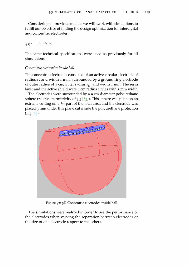
4.5 multilayer coplanar capacitive electrodes 129
Considering all previous models we will work with simulations tofulfill our objective of finding the design optimization for interdigitaland concentric electrodes.
4.5.2 Simulation
The same technical specifications were used as previously for allsimulations
Concentric electrodes inside ball
The concentric electrodes consisted of an active circular electrode ofradius ra and width 1 mm, surrounded by a ground ring electrodeof outer radius of 3 cm, inner radius rg,i and width 1 mm. The resinlayer and the active shield were 6 cm radius circles with 1 mm width.
The electrodes were surrounded by a 9 cm diameter polyurethanesphere (relative permittivity of 3.3 [63]). This sphere was plain on anextreme cutting off a 1/4 part of the total area, and the electrode wasplaced 3 mm under this plane cut inside the polyurethane protection(Fig. 97).
Figure 97: 3D Concentric electrodes inside ball
The simulations were realized in order to see the performance ofthe electrodes when varying the separation between electrodes orthe size of one electrode respect to the others.
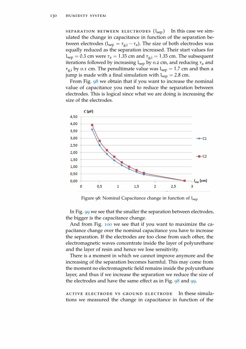
130 humidity system
separation between electrodes (lsep ) In this case we sim-ulated the change in capacitance in function of the separation be-tween electrodes (lsep = rg,i − ra). The size of both electrodes wasequally reduced as the separation increased. Their start values forlsep = 0.3 cm were ra = 1.35 cm and rg,i = 1.35 cm. The subsequentiterations followed by increasing lsep by 0.2 cm, and reducing ra andrg,i by 0.1 cm. The penultimate value was lsep = 1.7 cm and then ajump is made with a final simulation with lsep = 2.8 cm.
From Fig. 98 we obtain that if you want to increase the nominalvalue of capacitance you need to reduce the separation betweenelectrodes. This is logical since what we are doing is increasing thesize of the electrodes.
Figure 98: Nominal Capacitance change in function of lsep
In Fig. 99 we see that the smaller the separation between electrodes,the bigger is the capacitance change.
And from Fig. 100 we see that if you want to maximize the ca-pacitance change over the nominal capacitance you have to increasethe separation. If the electrodes are too close from each other, theelectromagnetic waves concentrate inside the layer of polyurethaneand the layer of resin and hence we lose sensitivity.
There is a moment in which we cannot improve anymore and theincreasing of the separation becomes harmful. This may come fromthe moment no electromagnetic field remains inside the polyurethanelayer, and thus if we increase the separation we reduce the size ofthe electrodes and have the same effect as in Fig. 98 and 99.
active electrode vs ground electrode In these simula-tions we measured the change in capacitance in function of the
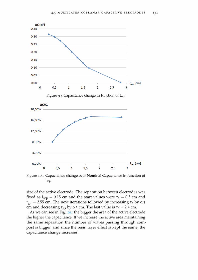
4.5 multilayer coplanar capacitive electrodes 131
Figure 99: Capacitance change in function of lsep
Figure 100: Capacitance change over Nominal Capacitance in function oflsep
size of the active electrode. The separation between electrodes wasfixed as lsep = 0.15 cm and the start values were ra = 0.3 cm andrg,i = 2.55 cm. The next iterations followed by increasing ra by 0.3cm and decreasing rg,i by 0.3 cm. The last value is ra = 2.4 cm.
As we can see in Fig. 101 the bigger the area of the active electrodethe higher the capacitance. If we increase the active area maintainingthe same separation the number of waves passing through com-post is bigger, and since the resin layer effect is kept the same, thecapacitance change increases.
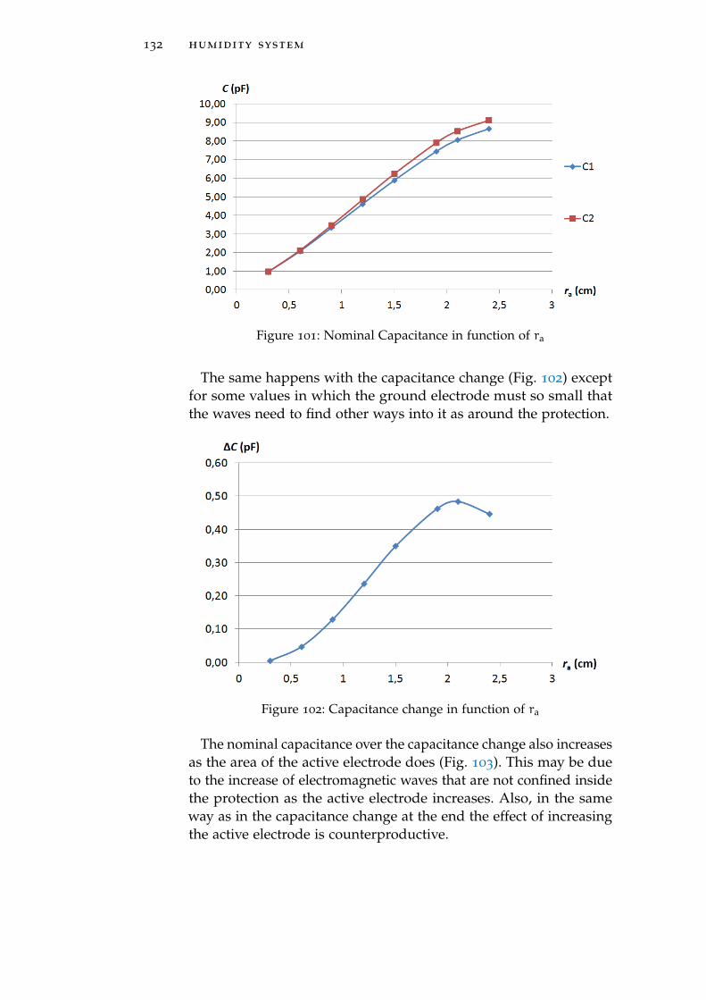
132 humidity system
Figure 101: Nominal Capacitance in function of ra
The same happens with the capacitance change (Fig. 102) exceptfor some values in which the ground electrode must so small thatthe waves need to find other ways into it as around the protection.
Figure 102: Capacitance change in function of ra
The nominal capacitance over the capacitance change also increasesas the area of the active electrode does (Fig. 103). This may be dueto the increase of electromagnetic waves that are not confined insidethe protection as the active electrode increases. Also, in the sameway as in the capacitance change at the end the effect of increasingthe active electrode is counterproductive.
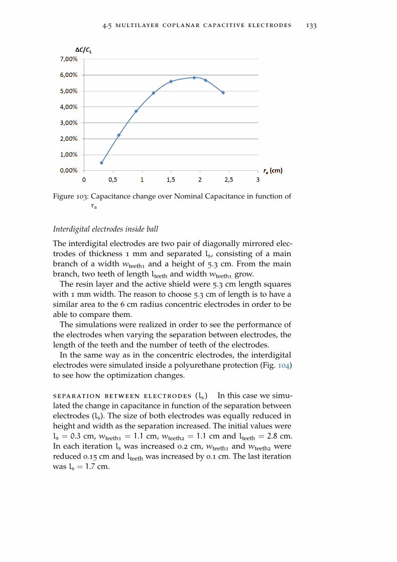
4.5 multilayer coplanar capacitive electrodes 133
Figure 103: Capacitance change over Nominal Capacitance in function ofra
Interdigital electrodes inside ball
The interdigital electrodes are two pair of diagonally mirrored elec-trodes of thickness 1 mm and separated ls, consisting of a mainbranch of a width wteeth1
and a height of 5.3 cm. From the mainbranch, two teeth of length lteeth and width wteeth1
grow.The resin layer and the active shield were 5.3 cm length squares
with 1 mm width. The reason to choose 5.3 cm of length is to have asimilar area to the 6 cm radius concentric electrodes in order to beable to compare them.
The simulations were realized in order to see the performance ofthe electrodes when varying the separation between electrodes, thelength of the teeth and the number of teeth of the electrodes.
In the same way as in the concentric electrodes, the interdigitalelectrodes were simulated inside a polyurethane protection (Fig. 104)to see how the optimization changes.
separation between electrodes (ls ) In this case we simu-lated the change in capacitance in function of the separation betweenelectrodes (ls). The size of both electrodes was equally reduced inheight and width as the separation increased. The initial values werels = 0.3 cm, wteeth1
= 1.1 cm, wteeth2= 1.1 cm and lteeth = 2.8 cm.
In each iteration ls was increased 0.2 cm, wteeth1and wteeth2
werereduced 0.15 cm and lteeth was increased by 0.1 cm. The last iterationwas ls = 1.7 cm.
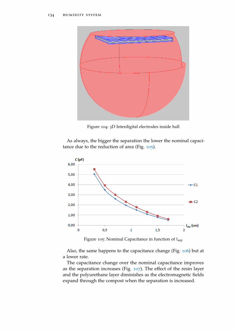
134 humidity system
Figure 104: 3D Interdigital electrodes inside ball
As always, the bigger the separation the lower the nominal capaci-tance due to the reduction of area (Fig. 105).
Figure 105: Nominal Capacitance in function of lsep
Also, the same happens to the capacitance change (Fig. 106) but ata lower rate.
The capacitance change over the nominal capacitance improvesas the separation increases (Fig. 107). The effect of the resin layerand the polyurethane layer diminishes as the electromagnetic fieldsexpand through the compost when the separation is increased.
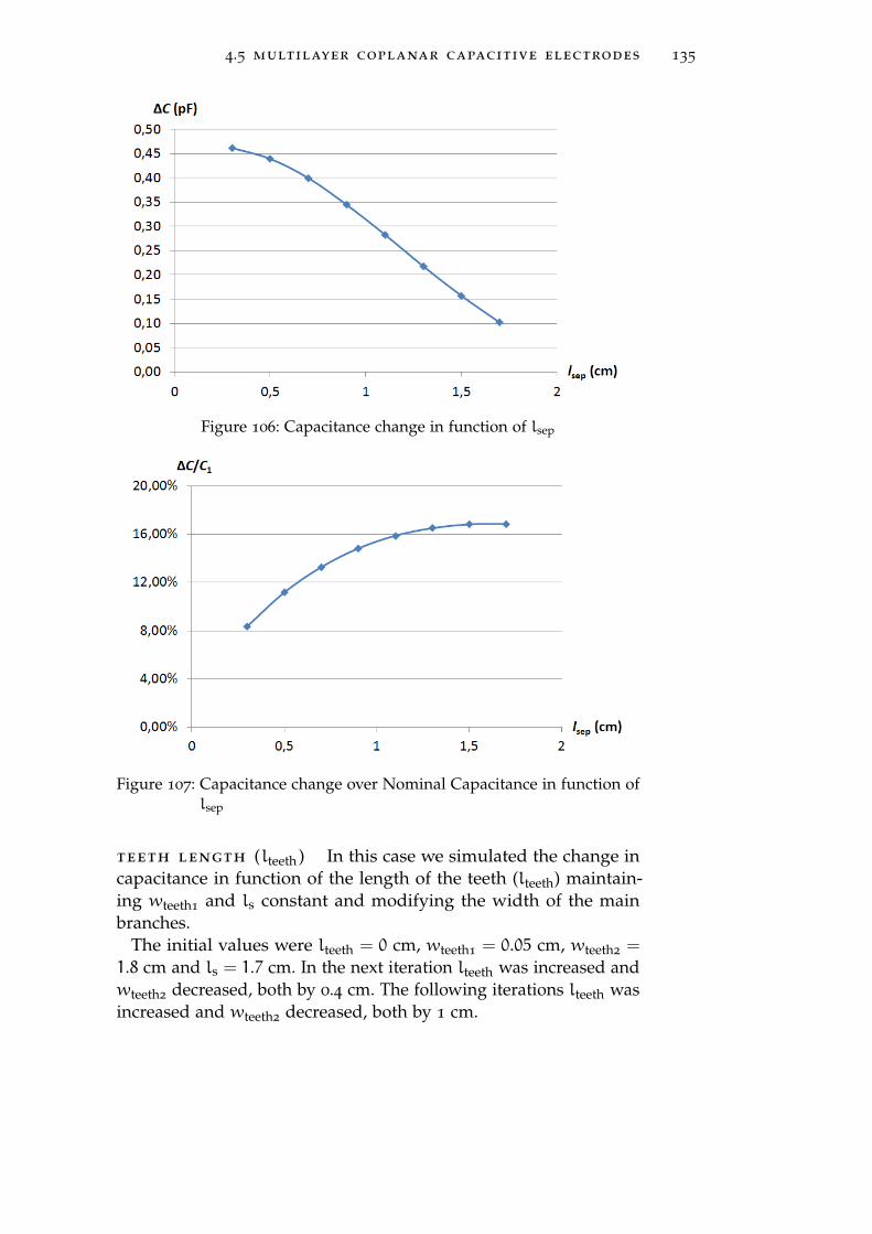
4.5 multilayer coplanar capacitive electrodes 135
Figure 106: Capacitance change in function of lsep
Figure 107: Capacitance change over Nominal Capacitance in function oflsep
teeth length (lteeth ) In this case we simulated the change incapacitance in function of the length of the teeth (lteeth) maintain-ing wteeth1
and ls constant and modifying the width of the mainbranches.
The initial values were lteeth = 0 cm, wteeth1= 0.05 cm, wteeth2
=
1.8 cm and ls = 1.7 cm. In the next iteration lteeth was increased andwteeth2
decreased, both by 0.4 cm. The following iterations lteeth wasincreased and wteeth2
decreased, both by 1 cm.
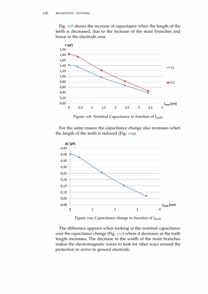
136 humidity system
Fig. 108 shows the increase of capacitance when the length of theteeth is decreased, due to the increase of the main branches andhence in the electrode area.
Figure 108: Nominal Capacitance in function of lteeth
For the same reason the capacitance change also increases whenthe length of the teeth is reduced (Fig. 109).
Figure 109: Capacitance change in function of lteeth
The difference appears when looking at the nominal capacitanceover the capacitance change (Fig. 110) where it decreases as the teethlength increases. The decrease in the width of the main branchesmakes the electromagnetic waves to look for other ways around theprotection to arrive to ground electrode.
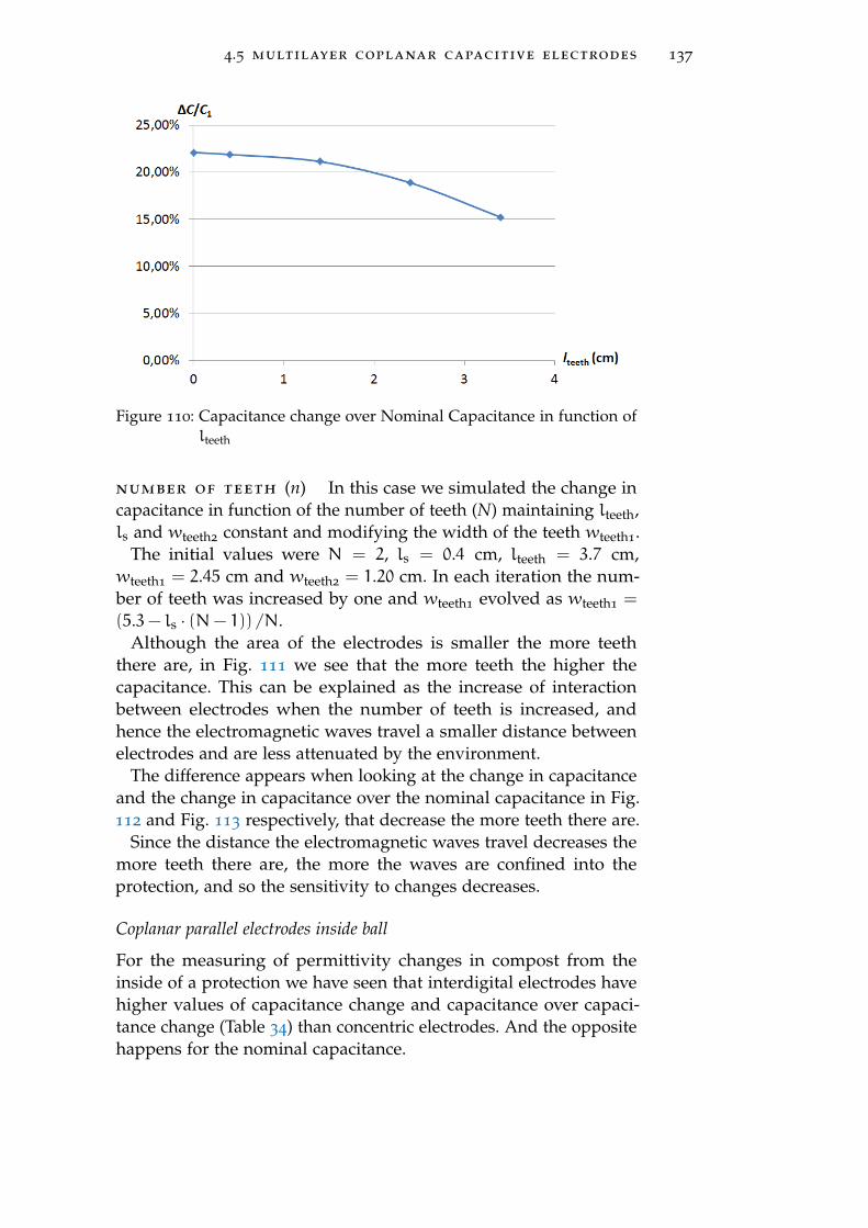
4.5 multilayer coplanar capacitive electrodes 137
Figure 110: Capacitance change over Nominal Capacitance in function oflteeth
number of teeth (n) In this case we simulated the change incapacitance in function of the number of teeth (N) maintaining lteeth,ls and wteeth2
constant and modifying the width of the teeth wteeth1.
The initial values were N = 2, ls = 0.4 cm, lteeth = 3.7 cm,wteeth1
= 2.45 cm and wteeth2= 1.20 cm. In each iteration the num-
ber of teeth was increased by one and wteeth1evolved as wteeth1
=
(5.3− ls · (N− 1)) /N.Although the area of the electrodes is smaller the more teeth
there are, in Fig. 111 we see that the more teeth the higher thecapacitance. This can be explained as the increase of interactionbetween electrodes when the number of teeth is increased, andhence the electromagnetic waves travel a smaller distance betweenelectrodes and are less attenuated by the environment.
The difference appears when looking at the change in capacitanceand the change in capacitance over the nominal capacitance in Fig.112 and Fig. 113 respectively, that decrease the more teeth there are.
Since the distance the electromagnetic waves travel decreases themore teeth there are, the more the waves are confined into theprotection, and so the sensitivity to changes decreases.
Coplanar parallel electrodes inside ball
For the measuring of permittivity changes in compost from theinside of a protection we have seen that interdigital electrodes havehigher values of capacitance change and capacitance over capaci-tance change (Table 34) than concentric electrodes. And the oppositehappens for the nominal capacitance.
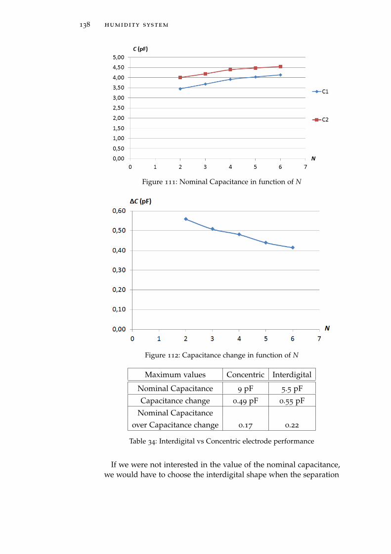
138 humidity system
Figure 111: Nominal Capacitance in function of N
Figure 112: Capacitance change in function of N
Maximum values Concentric Interdigital
Nominal Capacitance 9 pF 5.5 pF
Capacitance change 0.49 pF 0.55 pF
Nominal Capacitanceover Capacitance change 0.17 0.22
Table 34: Interdigital vs Concentric electrode performance
If we were not interested in the value of the nominal capacitance,we would have to choose the interdigital shape when the separation
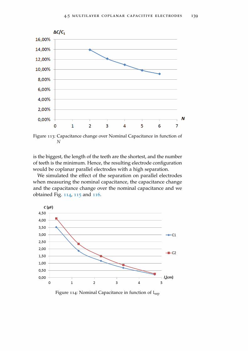
4.5 multilayer coplanar capacitive electrodes 139
Figure 113: Capacitance change over Nominal Capacitance in function ofN
is the biggest, the length of the teeth are the shortest, and the numberof teeth is the minimum. Hence, the resulting electrode configurationwould be coplanar parallel electrodes with a high separation.
We simulated the effect of the separation on parallel electrodeswhen measuring the nominal capacitance, the capacitance changeand the capacitance change over the nominal capacitance and weobtained Fig. 114, 115 and 116.
Figure 114: Nominal Capacitance in function of lsep
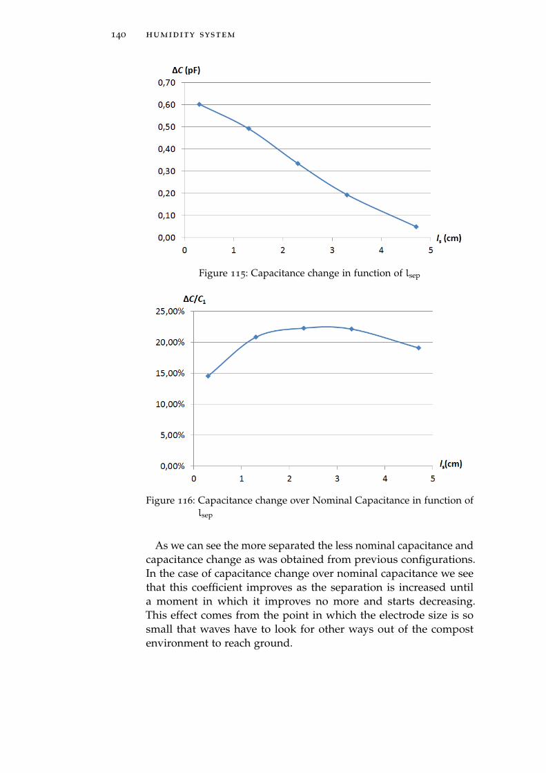
140 humidity system
Figure 115: Capacitance change in function of lsep
Figure 116: Capacitance change over Nominal Capacitance in function oflsep
As we can see the more separated the less nominal capacitance andcapacitance change as was obtained from previous configurations.In the case of capacitance change over nominal capacitance we seethat this coefficient improves as the separation is increased untila moment in which it improves no more and starts decreasing.This effect comes from the point in which the electrode size is sosmall that waves have to look for other ways out of the compostenvironment to reach ground.
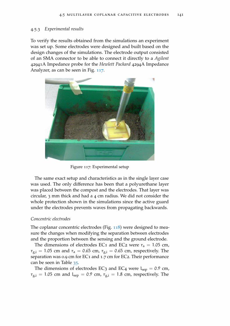
4.5 multilayer coplanar capacitive electrodes 141
4.5.3 Experimental results
To verify the results obtained from the simulations an experimentwas set up. Some electrodes were designed and built based on thedesign changes of the simulations. The electrode output consistedof an SMA connector to be able to connect it directly to a Agilent42941A Impedance probe for the Hewlett Packard 4294A ImpedanceAnalyzer, as can be seen in Fig. 117.
Figure 117: Experimental setup
The same exact setup and characteristics as in the single layer casewas used. The only difference has been that a polyurethane layerwas placed between the compost and the electrodes. That layer wascircular, 3 mm thick and had a 4 cm radius. We did not consider thewhole protection shown in the simulations since the active guardunder the electrodes prevents waves from propagating backwards.
Concentric electrodes
The coplanar concentric electrodes (Fig. 118) were designed to mea-sure the changes when modifying the separation between electrodesand the proportion between the sensing and the ground electrode.
The dimensions of electrodes EC1 and EC2 were ra = 1.05 cm,rg,i = 1.05 cm and ra = 0.65 cm, rg,i = 0.65 cm, respectively. Theseparation was 0.9 cm for EC1 and 1.7 cm for EC2. Their performancecan be seen in Table 35.
The dimensions of electrodes EC3 and EC4 were lsep = 0.9 cm,rg,i = 1.05 cm and lsep = 0.9 cm, rg,i = 1.8 cm, respectively. The

142 humidity system
Figure 118: Experimental concentric electrodes
lsep C1 (pF) C2 (pF) 4C (pF) 4C/C1 (%)
0.9 cm 6.97 8.17 1.20 17.20
1.7 cm 6.49 7.64 1.15 17.60
lsep ↑ ↓ ↓ ↓ ↑
Table 35: Concentric electrodes experimental performance in function oflsep
radius of the sensing electrode was 0.3 cm for EC3 and 1.8 cm forEC4. Their performance can be seen in Table 36.
ra C1 (pF) C2 (pF) 4C (pF) 4C/C1 (%)
0.3 cm 7.94 1.02 2.29 28.8
1.8 cm 7.98 1.06 2.66 33.3
ra ↑ ↑ ↑ ↑ ↑
Table 36: Concentric electrodes experimental performance in function of ra
As can be seen the behavior of modifying the separation or the pro-portion in the sizes between the sensing and the ground electrodes,is the same as seen in the simulations. The nominal capacitance ishigher in the experimental case since the density of the compost ismuch higher, hence the slope of the humidity/permittivity line ishigher the higher the density.
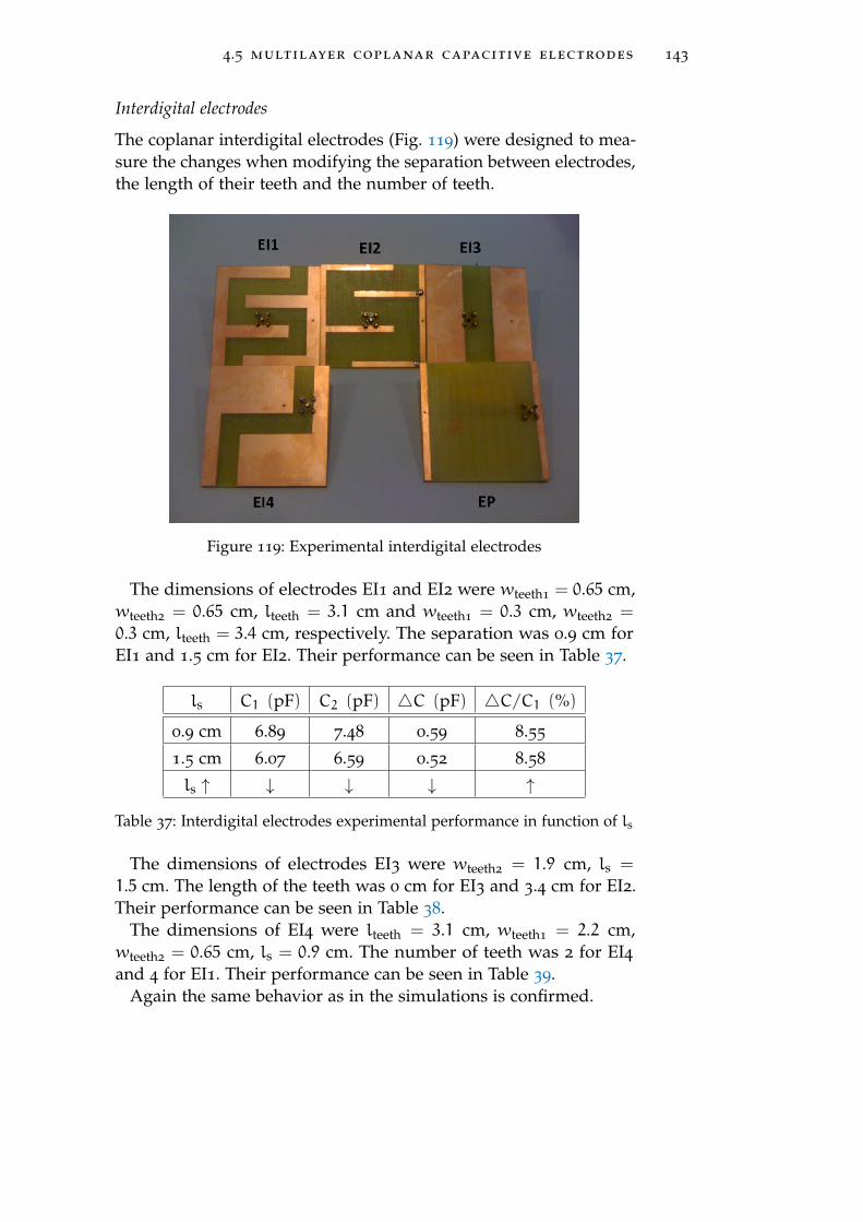
4.5 multilayer coplanar capacitive electrodes 143
Interdigital electrodes
The coplanar interdigital electrodes (Fig. 119) were designed to mea-sure the changes when modifying the separation between electrodes,the length of their teeth and the number of teeth.
Figure 119: Experimental interdigital electrodes
The dimensions of electrodes EI1 and EI2 were wteeth1= 0.65 cm,
wteeth2= 0.65 cm, lteeth = 3.1 cm and wteeth1
= 0.3 cm, wteeth2=
0.3 cm, lteeth = 3.4 cm, respectively. The separation was 0.9 cm forEI1 and 1.5 cm for EI2. Their performance can be seen in Table 37.
ls C1 (pF) C2 (pF) 4C (pF) 4C/C1 (%)
0.9 cm 6.89 7.48 0.59 8.55
1.5 cm 6.07 6.59 0.52 8.58
ls ↑ ↓ ↓ ↓ ↑
Table 37: Interdigital electrodes experimental performance in function of ls
The dimensions of electrodes EI3 were wteeth2= 1.9 cm, ls =
1.5 cm. The length of the teeth was 0 cm for EI3 and 3.4 cm for EI2.Their performance can be seen in Table 38.
The dimensions of EI4 were lteeth = 3.1 cm, wteeth1= 2.2 cm,
wteeth2= 0.65 cm, ls = 0.9 cm. The number of teeth was 2 for EI4
and 4 for EI1. Their performance can be seen in Table 39.Again the same behavior as in the simulations is confirmed.
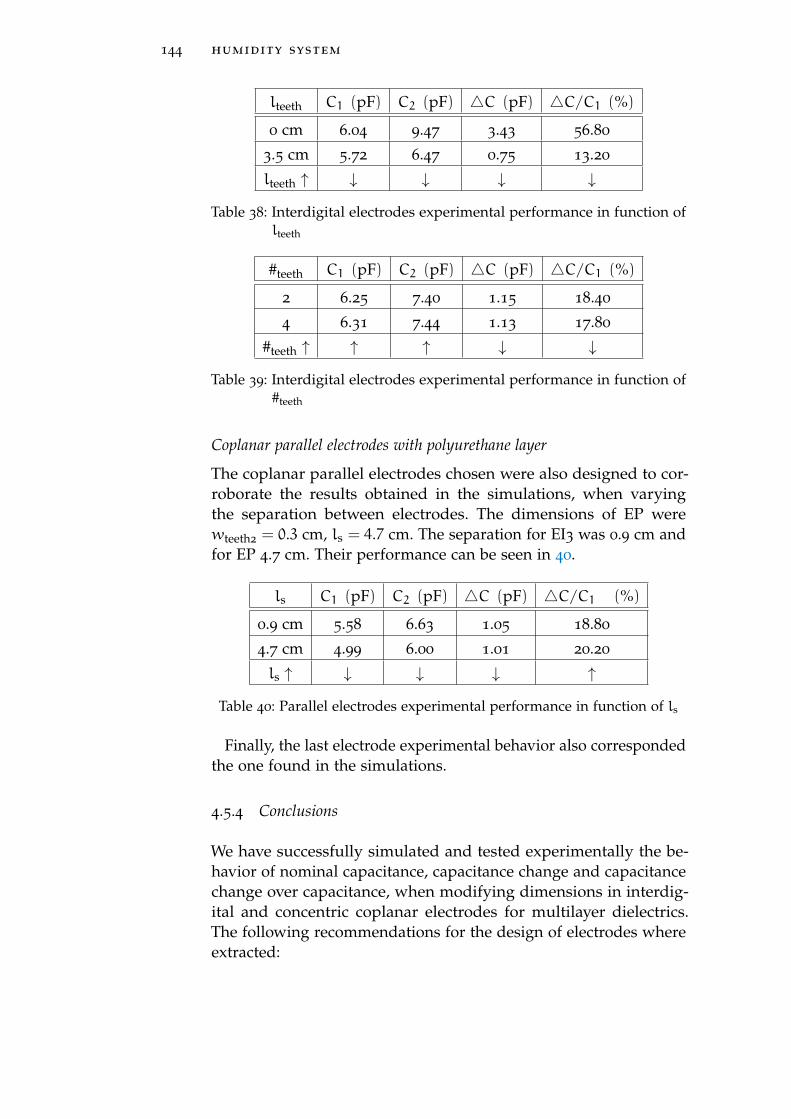
144 humidity system
lteeth C1 (pF) C2 (pF) 4C (pF) 4C/C1 (%)
0 cm 6.04 9.47 3.43 56.80
3.5 cm 5.72 6.47 0.75 13.20
lteeth ↑ ↓ ↓ ↓ ↓
Table 38: Interdigital electrodes experimental performance in function oflteeth
#teeth C1 (pF) C2 (pF) 4C (pF) 4C/C1 (%)
2 6.25 7.40 1.15 18.40
4 6.31 7.44 1.13 17.80
#teeth ↑ ↑ ↑ ↓ ↓
Table 39: Interdigital electrodes experimental performance in function of#teeth
Coplanar parallel electrodes with polyurethane layer
The coplanar parallel electrodes chosen were also designed to cor-roborate the results obtained in the simulations, when varyingthe separation between electrodes. The dimensions of EP werewteeth2
= 0.3 cm, ls = 4.7 cm. The separation for EI3 was 0.9 cm andfor EP 4.7 cm. Their performance can be seen in 40.
ls C1 (pF) C2 (pF) 4C (pF) 4C/C1 (%)
0.9 cm 5.58 6.63 1.05 18.80
4.7 cm 4.99 6.00 1.01 20.20
ls ↑ ↓ ↓ ↓ ↑
Table 40: Parallel electrodes experimental performance in function of ls
Finally, the last electrode experimental behavior also correspondedthe one found in the simulations.
4.5.4 Conclusions
We have successfully simulated and tested experimentally the be-havior of nominal capacitance, capacitance change and capacitancechange over capacitance, when modifying dimensions in interdig-ital and concentric coplanar electrodes for multilayer dielectrics.The following recommendations for the design of electrodes whereextracted:
4.6 final electrode calibration 145
We could use concentric electrodes to have the biggest nominalcapacitance and the sensitivity (4C) when the predominant distur-bance is the noise of the system and also to avoid corner effects. Ifwe wanted them for the first thing then we need to decrease theseparation and to increase the sensing electrode as much as possible.If we wanted them only for the second reason then, to increase thesensitivity when the error depends on the relative permittivity, weneed to increase the separation and the sensing electrode, avoidingthe limit cases which produce the opposite effect.
We will use parallel electrodes to have the biggest relative sensitiv-ity (4C/C1) since the the predominant disturbance is the inaccuracydue to the heterogeneity of the material. To do so we need to increasethe separation as much as possible without reaching the limits. Alsowe have to be careful since these electrode design is the one withthe lowest nominal capacitance.
4.6 final electrode calibration
Coplanar parallel electrode have the highest sensitivity when theseparation is not too big nor too small. However, as explained before,the higher the sensing sensitivity the higher the sensitivity error. Wehave determined that the best error-sensitivity relation appears whenthe separation is as big as possible. And, although experimentallythe nominal capacitance has resulted bigger than 1 pF, theoreticallythis value can be smaller1. As such, it has been determined thatthe suitable electrodes for our application would be the coplanarparallel electrodes with a separation of 0.9 cm.
Now we will calibrate the geometry factor of these electrodes bycalibrating them.
If we calculate the relative permittivity of C1 = 5.58 pF withequation (4.6) and then we calculate the calibration factor (Kc · Γ )with Equation 4.1 we obtain a value of 0.0437.
If we do the same for C2 = 6.63 pF we obtain a calibration factorof 0.0383. As we can see the difference between the two calibratedfactors is considerably big (a 12.36 % difference). This is normaldue to what we said at the beginning of the chapter, compost is avery heterogeneous material and Equation 4.1 answers to a singledielectric. To this we can add the error in the calculation of humiditywith the moisture analyzer. As said in the first chapter, currentcommercial humidity sensors are accurate within a 5-10% margin,
1 We have to take into account that the compost used in the experimental setupwas much more dense than the supposed in the simulations which would betranslated as a relative permittivity of around 20.
146 humidity system
and as such their measure may have caused the calibration factor tovary between a 5 and 10 %.
In our case, to reduce the uncertainty, we can average the cali-bration factor to obtain a better reference. Obviously, with moresamples the calibration factor uncertainty could be reduced more. Apart, we should do a calibration curve dependent on the humiditylevel.
4.7 electrode design conclusion
We have obtained a theoretical model for the calculation of thecapacitance for concentric and interdigital electrodes. This modelcan be used to calculate the relative permitivity of a material incontact with the elctrodes. If a protective layer is put between theelectrodes and the material under test then the theoretical modelwould measure the permittivity of both materials.
The theoretical model can be used to see what kind of concentricor interdigital electrode would be more suitable for a specific ap-plication. Nevertheless, some recommendations for the design ofelectrodes have been extrapolated in function of their application:
If the electrodes will be in direct contact with the dielectric under test
You can use concentric electrodes to have the biggest nominal capac-itance and the biggest sensitivity when the noise does not changein function of the relative permittivity, and to avoid corner effects.Whether you are interested on one of their advantages or all of them,you have to take into account that if you want to have the highestsensitivity you need to decrease the separation between electrodesand to make the sensing electrode much bigger than the groundelectrode. In the case you want the highest sensitivity when thenoise depends on the relative permittivity, you need to increase theseparation as much as possible.
You can use interdigital electrodes to have the biggest sensitivitywhen the noise changes in function of the relative permittivity. Inthat case you need to increase the separation between electrodes, thelength of the teeth and the number of teeth.
If the electrodes have a protective layer
You can use concentric electrodes to have the biggest sensitivitywhen the noise does not change in function of the relative permittiv-ity, and to avoid corner effects. If you want them for the first thingthen you need to decrease the separation and to increase the sensing
4.7 electrode design conclusion 147
electrode as much as possible. If you want them only for the secondreason then, to increase the sensitivity when the error depends onthe relative permittivity, you need to increase the separation andthe sensing electrode, avoiding the limit cases which produce theopposite effect.
You can use parallel electrodes to have the biggest sensitivity whenthe noise changes in function of the relative permittivity. To do so yoneed to increase the separation as much as possible without reachingthe limits. Also yo have to be careful since these electrode design isthe one with the lowest nominal capacitance.
Others
If you can change the size of the electrodes then choose to makethem bigger, not only to increase their nominal capacitance, but alsotheir sensitivity. Also if you want to mix characteristics of electrodesyou could design hybrids electrodes, e.g. a concentric interdigitalelectrode to avoid corner effects and to increase the sensitivity asmuch as possible when the electrode is not in direct contact withthe dielectric under test.
It’s more fun to arrive a conclusion than to justify it.
— Malcolm Forbes, pulbisher
5C O N C L U S I O N S
Along the development of this thesis compost has been proved to bea very complex material for monitoring, study and characterization.As follows we will detail conclusions for the different objectives ofthe project and for the overall thesis.
First of all, a temperature system has been developed embeddedinto a protective material able to measure and record temperature, tooperate inside a compost pile (or whichever enclosure we were using)for at least two months recording samples every half an hour. Wefound that the protective material delayed the thermal conductivityand the measured temperature followed the compost temperaturewith a first order delay. To compensate this effect an algorithmimplementable in microcontrollers was developed to calculate thethe tendency of the first order (this method allows the final value tobe found in 65 % of the time required using the first-order systemgeneric equation for an error lower than 0.1 %, or 59 % of the timefor an error lower than 1 %). To be able to have an autonomoussystem we applied different techniques for consumption saving; oneof them was the direct sensor-to-microcontroller interface which weproved to consume much less than classic conditioning at the costof some resolution. At the end, our system was able to successfullymeasure through an experiment on a compost pile for two months(although it could have last longer).
Secondly, the wireless communication in compost was studiedto remotely send the measures to the operator without any inter-vention in the monitoring system.We saw that the attenuation incompost was bigger than in air or soil, and that it increased with thefrequency. Still, we found that for lower bands (under 500 MHz) thecommunications were possible for distances around 10 m. We de-cided to use the 433 MHz free band for the transmission in compostmainly for its good relation attenuation/consumption and becauseof the availability of transmitting devices at this frequency band.We developed experiments to see what was the attenuation of 433
MHz antennas, inside of the protective capsule, in function of the
148
conclusions 149
distance. We saw that the protective layer detuned the antenna anddisplaced the design frequency which we propose that could becompensated through a tuning circuit connected to the antenna. Wealso saw that the attenuation of compost was inversely proportionalto the distance elevated to 3. Some tests based on our study wererealized inside a compost pile and proved that a distance of 3 to 4
m allowed a proper transmission of information through compost.Finally, the optimal method of measure of the humidity of compost
from the inside of a protective capsule was studied. We developeda humidity sensor system based on the changes of a pair of copla-nar capacitive electrodes placed inside a capsule which allowed alocal measure of humidity with a low consumption. Before, though,we characterized the relative permittivity of compost to see howhumidity, density, temperature and salt content affected. We foundthat impedance measures of compost with capacitive electrodes atfrequencies from 25 MHz to 100 MHz allowed neglecting the effectof temperature and salt content. At the end we extracted an equationwhich described the relative permittivity of compost in function ofits humidity and density.
Regarding the shape and dimensions of the coplanar capacitiveelectrodes we simulated different cases for concentric and interdig-ital electrodes. The results of the simulations were modeled andan equation for each type was obtained. The simulations and theequations were compared to some lab experiments and their accept-able use for experimental cases was demonstrated. Together withthe equations some recommendations were defined to help designan optimum electrode in function of the disturbance sources. In ourcase, since we have a protective capsule and our main disturbance isthe uncertainty of the material under measure we would use parallelcoplanar electrodes increasing the separation as much as possiblewithout reaching the limits.

A P P E N D I X
151
AT E M P E R AT U R E S Y S T E M C O M P O N E N TS E L E C T I O N
As follows we will explain the rest of the components of the archi-tecture, their options and their justifications.
a.1 microcontroller
In order to manage and control any kind of system a brain is needed.This brain is not required to be complex, and for autonomous sys-tems as our application they can be as simple as a microcontroller.A microcontroller (also microcontroller unit, MCU or µC) is a smallcomputer on a single integrated circuit consisting of a relativelysimple CPU combined with support functions such as a crystaloscillator, timers, watchdog, serial and analogue I/O, etc [128].
There are many microcontroller manufacturers, but the most im-portant ones are Atmel Corporation, Microchip Technology and TexasInstruments. Focusing on the main manufacturers increases the avail-ability of the products, technical support disposal and the possibilityof obtaining samples.
Our microcontroller should have a flash memory over 8 kbits inorder to be able to implement an algorithm for controlling andmanaging the whole system. This number was found from theexperience on the design of a previous temperature system, in whichan 8 kbit capacity was needed to implement its algorithm[129].
To be able to download and upload data between the microcon-troller and a computer, a serial UART is needed. A part, in orderto communicate with the real time clock and the EEPROM devicesan i2C bus interface is required. I2C uses the typical master-slavearchitecture of the microcontroller systems. Unlike the CAN businterfaces, the i2C consumption is lower and its transmission speedis bigger.
As will be explained in the sensor conditioning section, in orderto use the direct sensor-to-microcontroller interface, as the signalconditioning method, an external interruption port with an Schmitttrigger integrated is needed. Nowadays, all new microcontrollers dohave this feature, but when searching it is important to make it sure.
When looking for the specifications we need within the Atmelproducts we found many MCU fulfilling them. The lowest prize was
152
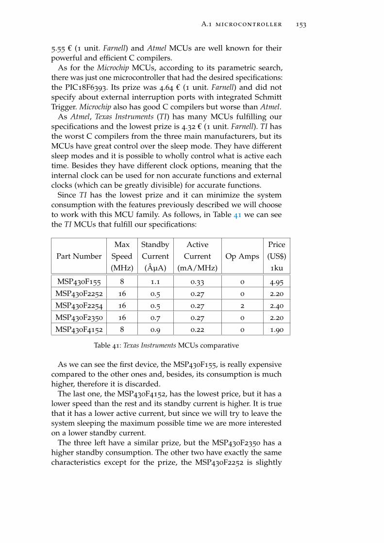
A.1 microcontroller 153
5.55 € (1 unit. Farnell) and Atmel MCUs are well known for theirpowerful and efficient C compilers.
As for the Microchip MCUs, according to its parametric search,there was just one microcontroller that had the desired specifications:the PIC18F6393. Its prize was 4.64 € (1 unit. Farnell) and did notspecify about external interruption ports with integrated SchmittTrigger. Microchip also has good C compilers but worse than Atmel.
As Atmel, Texas Instruments (TI) has many MCUs fulfilling ourspecifications and the lowest prize is 4.32 € (1 unit. Farnell). TI hasthe worst C compilers from the three main manufacturers, but itsMCUs have great control over the sleep mode. They have differentsleep modes and it is possible to wholly control what is active eachtime. Besides they have different clock options, meaning that theinternal clock can be used for non accurate functions and externalclocks (which can be greatly divisible) for accurate functions.
Since TI has the lowest prize and it can minimize the systemconsumption with the features previously described we will chooseto work with this MCU family. As follows, in Table 41 we can seethe TI MCUs that fulfill our specifications:
Max Standby Active PricePart Number Speed Current Current Op Amps (US$)
(MHz) (µA) (mA/MHz) 1ku
MSP430F155 8 1.1 0.33 0 4.95
MSP430F2252 16 0.5 0.27 0 2.20
MSP430F2254 16 0.5 0.27 2 2.40
MSP430F2350 16 0.7 0.27 0 2.20
MSP430F4152 8 0.9 0.22 0 1.90
Table 41: Texas Instruments MCUs comparative
As we can see the first device, the MSP430F155, is really expensivecompared to the other ones and, besides, its consumption is muchhigher, therefore it is discarded.
The last one, the MSP430F4152, has the lowest price, but it has alower speed than the rest and its standby current is higher. It is truethat it has a lower active current, but since we will try to leave thesystem sleeping the maximum possible time we are more interestedon a lower standby current.
The three left have a similar prize, but the MSP430F2350 has ahigher standby consumption. The other two have exactly the samecharacteristics except for the prize, the MSP430F2252 is slightly
154 temperature system component selection
cheaper, and that the MSP430F2254 has two internal operationalamplifiers. The prize is too similar and it is possible that the internaloperational amplifiers may become useful; therefore we decided toinitially use the MSP430F2254.
a.2 sensor
Resistance Temperature Detector (RTD), thermocouple, thermistor,and Integrated Circuit (IC) sensors are all useful temperature mea-surement options, with thermistors and IC sensors relegated tonarrower temperature ranges than RTDs and thermocouples.
RTDs provide higher accuracy because platinum is more stablethan most of the materials used in thermistors, thermocouples, andIC sensors. RTDs, thermistors, and IC sensors use standard instru-mentation wire to connect to the measurement or control equipment.Thermocouples, on the other hand, require special thermocoupleextension wire.
Thermocouples are generally less expensive than RTDs, but arecompetitive with thermistors and IC sensors in some applications.They are more durable in high-vibration or mechanical shock appli-cations, and are usable for measuring high temperatures. Becausethe different types of thermocouples are standardized, they can beeasily replaced when necessary.
Thermistors provide higher resolution than RTDs or thermocou-ples, and generally cost less. Their lower temperature range andnonlinearity limit their ability to work over large temperature excur-sions. Their low mass and small size give them quick response totemperature changes. The lack of standard resistance vs. temperaturecurves can cause difficulty in replacing sensors when needed.
IC and RTDs are linear sensors with a low prize, and an easyconditioning. For our application we need to have a good accuracylevel and IC temperature sensors do not fulfill this. Thermocoupleshave an even better accuracy than RTDs, but their special wirerequirements make them unsuitable for our setup. In Table 42 it ispossible to see some mayor commercial examples for each type oftemperature sensor. The RTD temperature chosen for our applicationis the Pt1000 which, besides, will allow using some new conditioningmethods.
a.3 real-time-clock (rtc)
To keep the track of the current time when the measurements ordifferent operations are realized, a Real-time-clock (RTC) is needed.
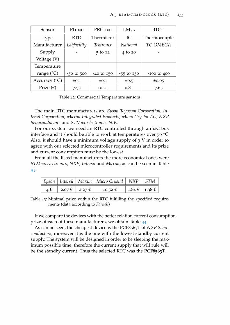
A.3 real-time-clock (rtc) 155
Sensor Pt1000 PRC 100 LM35 BTC-1
Type RTD Thermistor IC Thermocouple
Manufacturer Labfacility Tektronix National TC-OMEGASupply - 5 to 12 4 to 20 -
Voltage (V)
Temperaturerange (°C) -50 to 500 -40 to 150 -55 to 150 -100 to 400
Accuracy (°C) ±0.1 ±0.1 ±0.5 ±0.05
Prize (€) 7.53 10.31 0.81 7.65
Table 42: Commercial Temperature sensors
The main RTC manufacturers are Epson Toyocom Corporation, In-tersil Corporation, Maxim Integrated Products, Micro Crystal AG, NXPSemiconductors and STMicroelectronics N.V..
For our system we need an RTC controlled through an i2C businterface and it should be able to work at temperatures over 70
C.Also, it should have a minimum voltage supply of 3 V in order toagree with our selected microcontroller requirements and its prizeand current consumption must be the lowest.
From all the listed manufacturers the more economical ones wereSTMicroelectronics, NXP, Intersil and Maxim, as can be seen in Table43.
Epson Intersil Maxim Micro Crystal NXP STM
4 € 2.07 € 2.27 € 10.52 € 1.84 € 1.38 €
Table 43: Minimal prize within the RTC fulfilling the specified require-ments (data according to Farnell)
If we compare the devices with the better relation current consumption-prize of each of these manufacturers, we obtain Table 44.
As can be seen, the cheapest device is the PCF8563T of NXP Semi-conductors; moreover it is the one with the lowest standby currentsupply. The system will be designed in order to be sleeping the max-imum possible time, therefore the current supply that will rule willbe the standby current. Thus the selected RTC was the PCF8563T.
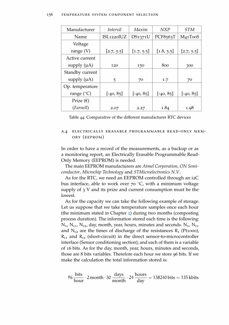
156 temperature system component selection
Manufacturer Intersil Maxim NXP STMName ISL1220IUZ DS1371U PCF8563T M41T00S
Voltagerange (V) [2.7, 5.5] [1.7, 5.5] [1.8, 5.5] [2.7, 5.5]
Active currentsupply (µA) 120 150 800 300
Standby currentsupply (µA) 5 70 1.7 70
Op. temperaturerange (C) [-40, 85] [-40, 85] [-40, 85] [-40, 85]
Prize (€)(Farnell) 2.07 2.27 1.84 1.98
Table 44: Comparative of the different manufacturer RTC devices
a.4 electrically erasable programmable read-only mem-ory (eeprom)
In order to have a record of the measurements, as a backup or asa monitoring report, an Electrically Erasable Programmable Read-Only Memory (EEPROM) is needed.
The main EEPROM manufacturers are Atmel Corporation, ON Semi-conductor, Microchip Technology and STMicroelectronics N.V..
As for the RTC, we need an EEPROM controlled through an i2Cbus interface, able to work over 70
C, with a minimum voltagesupply of 3 V and its prize and current consumption must be thelowest.
As for the capacity we can take the following example of storage.Let us suppose that we take temperature samples once each hour(the minimum stated in Chapter 2) during two months (compostingprocess duration). The information stored each time is the following:Nx, Nc1, Nc2, day, month, year, hours, minutes and seconds. Nx, Nc1
and Nc2 are the times of discharge of the resistances Rx (Pt1000),Rc1 and Rc2 (short-circuit) in the direct sensor-to-microcontrollerinterface (Sensor conditioning section); and each of them is a variableof 16 bits. As for the day, month, year, hours, minutes and seconds,those are 8 bits variables. Therefore each hour we store 96 bits. If wemake the calculation the total information stored is:
96bits
hour· 2month · 30 days
month· 24 hours
day= 138240 bits = 135 kbits
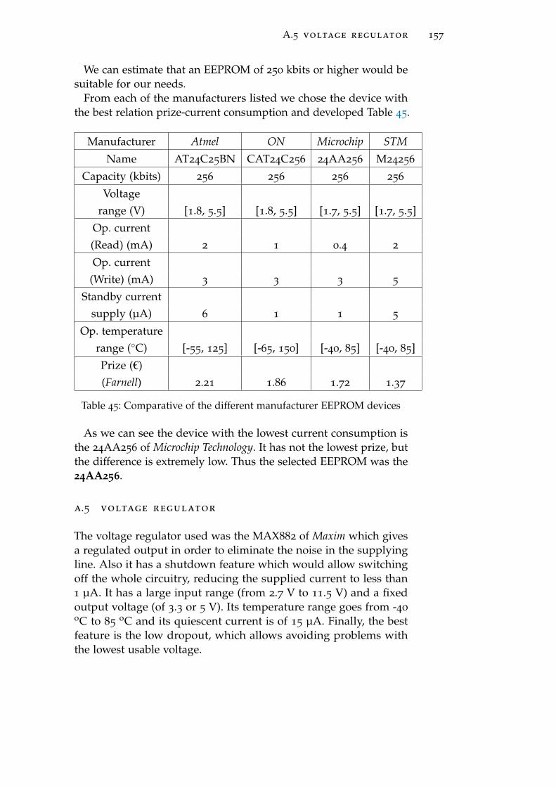
A.5 voltage regulator 157
We can estimate that an EEPROM of 250 kbits or higher would besuitable for our needs.
From each of the manufacturers listed we chose the device withthe best relation prize-current consumption and developed Table 45.
Manufacturer Atmel ON Microchip STMName AT24C25BN CAT24C256 24AA256 M24256
Capacity (kbits) 256 256 256 256
Voltagerange (V) [1.8, 5.5] [1.8, 5.5] [1.7, 5.5] [1.7, 5.5]
Op. current(Read) (mA) 2 1 0.4 2
Op. current(Write) (mA) 3 3 3 5
Standby currentsupply (µA) 6 1 1 5
Op. temperaturerange (C) [-55, 125] [-65, 150] [-40, 85] [-40, 85]
Prize (€)(Farnell) 2.21 1.86 1.72 1.37
Table 45: Comparative of the different manufacturer EEPROM devices
As we can see the device with the lowest current consumption isthe 24AA256 of Microchip Technology. It has not the lowest prize, butthe difference is extremely low. Thus the selected EEPROM was the24AA256.
a.5 voltage regulator
The voltage regulator used was the MAX882 of Maxim which givesa regulated output in order to eliminate the noise in the supplyingline. Also it has a shutdown feature which would allow switchingoff the whole circuitry, reducing the supplied current to less than1 µA. It has a large input range (from 2.7 V to 11.5 V) and a fixedoutput voltage (of 3.3 or 5 V). Its temperature range goes from -40
oC to 85oC and its quiescent current is of 15 µA. Finally, the best
feature is the low dropout, which allows avoiding problems withthe lowest usable voltage.
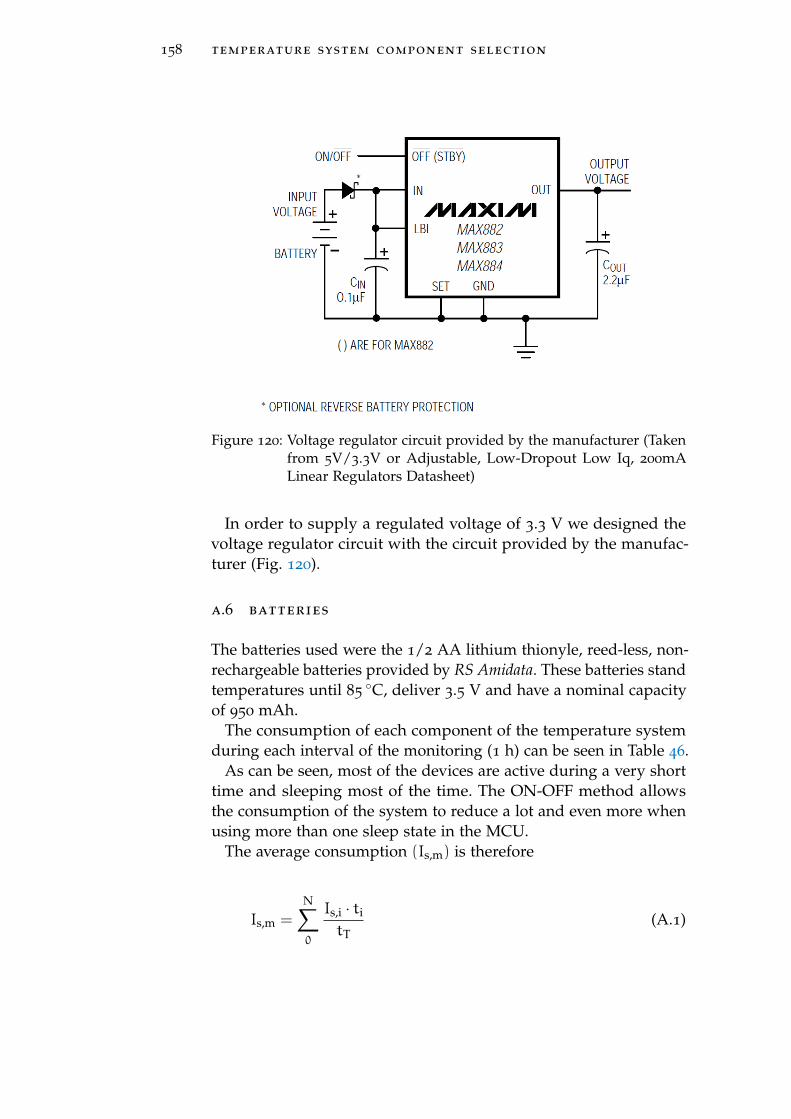
158 temperature system component selection
Figure 120: Voltage regulator circuit provided by the manufacturer (Takenfrom 5V/3.3V or Adjustable, Low-Dropout Low Iq, 200mALinear Regulators Datasheet)
In order to supply a regulated voltage of 3.3 V we designed thevoltage regulator circuit with the circuit provided by the manufac-turer (Fig. 120).
a.6 batteries
The batteries used were the 1/2 AA lithium thionyle, reed-less, non-rechargeable batteries provided by RS Amidata. These batteries standtemperatures until 85
C, deliver 3.5 V and have a nominal capacityof 950 mAh.
The consumption of each component of the temperature systemduring each interval of the monitoring (1 h) can be seen in Table 46.
As can be seen, most of the devices are active during a very shorttime and sleeping most of the time. The ON-OFF method allowsthe consumption of the system to reduce a lot and even more whenusing more than one sleep state in the MCU.
The average consumption (Is,m) is therefore
Is,m =
N∑0
Is,i · titT
(A.1)
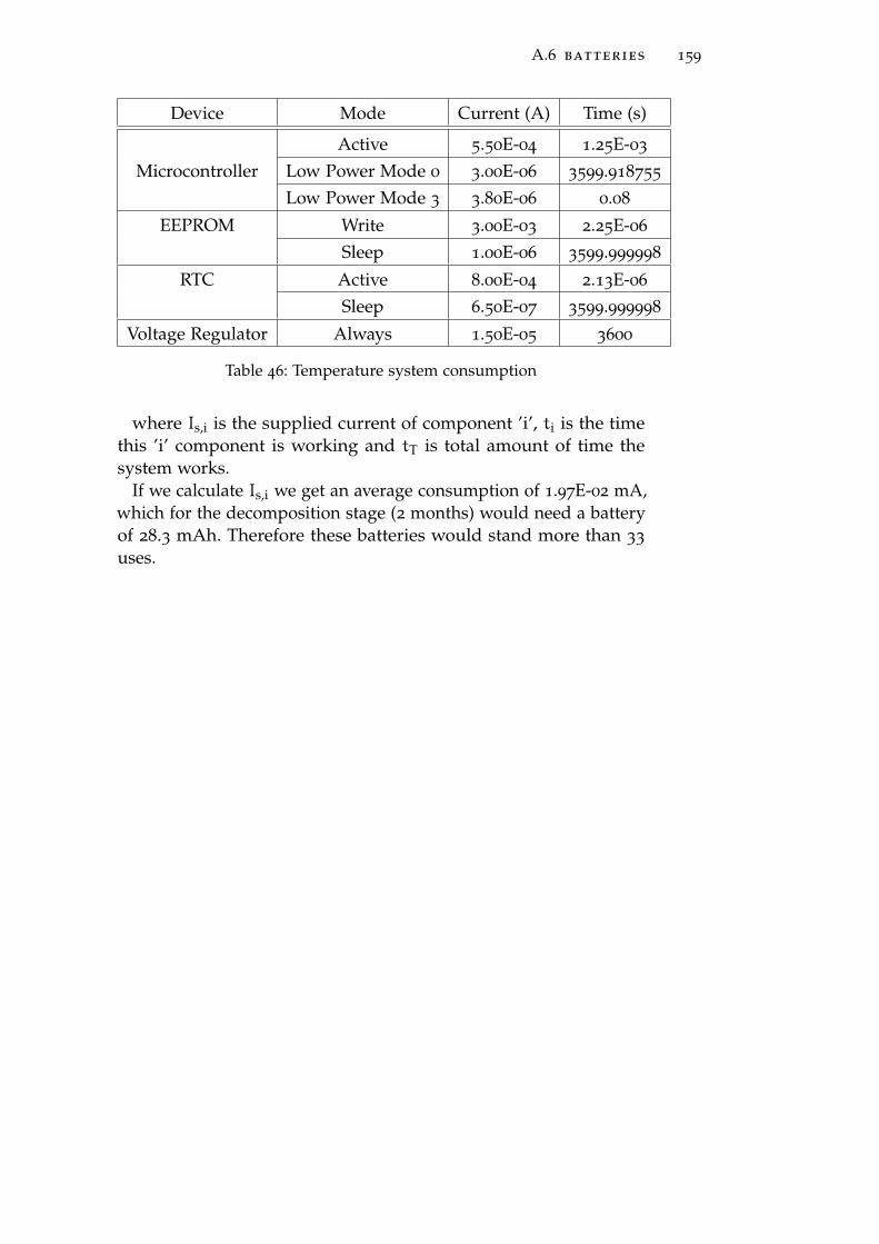
A.6 batteries 159
Device Mode Current (A) Time (s)
Active 5.50E-04 1.25E-03
Microcontroller Low Power Mode 0 3.00E-06 3599.918755
Low Power Mode 3 3.80E-06 0.08
EEPROM Write 3.00E-03 2.25E-06
Sleep 1.00E-06 3599.999998
RTC Active 8.00E-04 2.13E-06
Sleep 6.50E-07 3599.999998
Voltage Regulator Always 1.50E-05 3600
Table 46: Temperature system consumption
where Is,i is the supplied current of component ’i’, ti is the timethis ’i’ component is working and tT is total amount of time thesystem works.
If we calculate Is,i we get an average consumption of 1.97E-02 mA,which for the decomposition stage (2 months) would need a batteryof 28.3 mAh. Therefore these batteries would stand more than 33
uses.
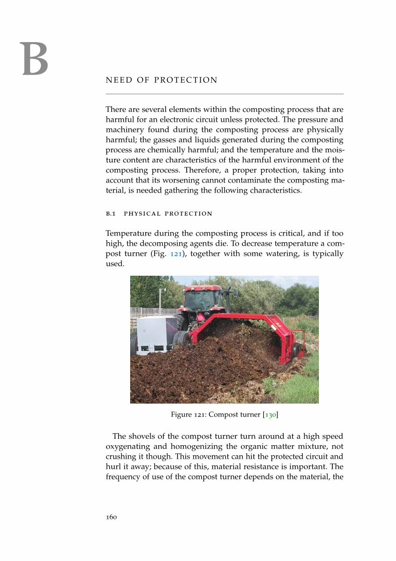
BN E E D O F P R O T E C T I O N
There are several elements within the composting process that areharmful for an electronic circuit unless protected. The pressure andmachinery found during the composting process are physicallyharmful; the gasses and liquids generated during the compostingprocess are chemically harmful; and the temperature and the mois-ture content are characteristics of the harmful environment of thecomposting process. Therefore, a proper protection, taking intoaccount that its worsening cannot contaminate the composting ma-terial, is needed gathering the following characteristics.
b.1 physical protection
Temperature during the composting process is critical, and if toohigh, the decomposing agents die. To decrease temperature a com-post turner (Fig. 121), together with some watering, is typicallyused.
Figure 121: Compost turner [130]
The shovels of the compost turner turn around at a high speedoxygenating and homogenizing the organic matter mixture, notcrushing it though. This movement can hit the protected circuit andhurl it away; because of this, material resistance is important. Thefrequency of use of the compost turner depends on the material, the
160
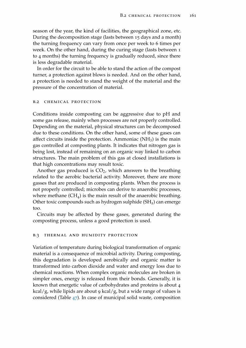
B.2 chemical protection 161
season of the year, the kind of facilities, the geographical zone, etc.During the decomposition stage (lasts between 15 days and a month)the turning frequency can vary from once per week to 6 times perweek. On the other hand, during the curing stage (lasts between 1
to 4 months) the turning frequency is gradually reduced, since thereis less degradable material.
In order for the circuit to be able to stand the action of the compostturner, a protection against blows is needed. And on the other hand,a protection is needed to stand the weight of the material and thepressure of the concentration of material.
b.2 chemical protection
Conditions inside composting can be aggressive due to pH andsome gas release, mainly when processes are not properly controlled.Depending on the material, physical structures can be decomposeddue to these conditions. On the other hand, some of these gases canaffect circuits inside the protection. Ammoniac (NH3) is the maingas controlled at composting plants. It indicates that nitrogen gas isbeing lost, instead of remaining on an organic way linked to carbonstructures. The main problem of this gas at closed installations isthat high concentrations may result toxic.
Another gas produced is CO2, which answers to the breathingrelated to the aerobic bacterial activity. Moreover, there are moregasses that are produced in composting plants. When the process isnot properly controlled; microbes can derive to anaerobic processes,where methane (CH4) is the main result of the anaerobic breathing.Other toxic compounds such as hydrogen sulphide (SH2) can emergetoo.
Circuits may be affected by these gases, generated during thecomposting process, unless a good protection is used.
b.3 thermal and humidity protection
Variation of temperature during biological transformation of organicmaterial is a consequence of microbial activity. During composting,this degradation is developed aerobically and organic matter istransformed into carbon dioxide and water and energy loss due tochemical reactions. When complex organic molecules are broken insimpler ones, energy is released from their bonds. Generally, it isknown that energetic value of carbohydrates and proteins is about 4
kcal/g, while lipids are about 9 kcal/g, but a wide range of values isconsidered (Table 47). In case of municipal solid waste, composition
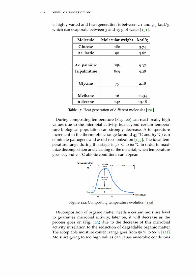
162 need of protection
is highly varied and heat generation is between 2.1 and 9.3 kcal/g,which can evaporate between 3 and 15 g of water [131].
Molecule Molecular weight kcal/g
Glucose 180 3.74
Ac. lactic 90 3.62
Ac. palmitic 256 9.37
Tripalmitine 809 9.28
Glycine 75 2.18
Methane 16 11.34
n-decane 142 13.18
Table 47: Heat generation of different molecules [132]
During composting temperature (Fig. 122) can reach really highvalues due to the microbial activity, but beyond certain tempera-ture biological population can strongly decrease. A temperatureincrement in the thermophilic range (around 45 °C and 65 °C) caneliminate pathogens and avoid recolonization [133]. The ideal tem-perature range during this stage is 50 °C to 60 °C in order to maxi-mize decomposition and cleaning of the material; when temperaturegoes beyond 70 °C abiotic conditions can appear.
Figure 122: Composting temperature evolution [132]
Decomposition of organic matter needs a certain moisture levelto guarantee microbial activity; later on, it will decrease as theprocess goes on (Fig. 123) due to the decrease of this microbialactivity in relation to the reduction of degradable organic matter.The acceptable moisture content range goes from 50 % to 60 % [132].Moisture going to too high values can cause anaerobic conditions
B.3 thermal and humidity protection 163
and excess of leachates and, consequently, the appearance of badodors.
Figure 123: Composting humidity evolution
After the active composting stage the curing phase follows. In thisstage the microbial activity slows down and as the process nearscompletion, the material approaches environment air temperature.Finished compost takes on many of the characteristics of humus, theorganic fraction of soil. The material will have its volume reducedby 20 % to 60 %, its moisture content by 40 % and its weight by upto 50 % from the initial material. It can be considered that, in anadequate process, from every 100 kg of raw material at the start ofthe process, around 25-35 kg of compost should be obtained.
The circuitry may operate at high temperatures during the com-posting process, but a minimal IP 67 protection is needed to protectagainst the humidity level.
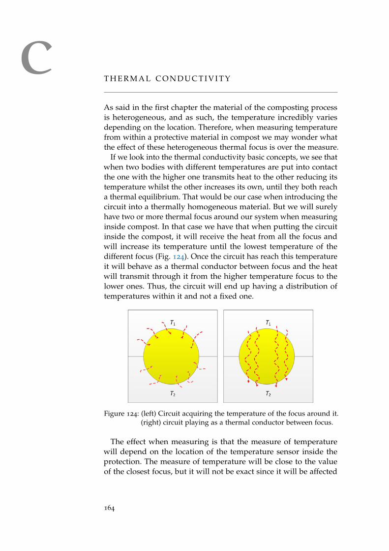
CT H E R M A L C O N D U C T I V I T Y
As said in the first chapter the material of the composting processis heterogeneous, and as such, the temperature incredibly variesdepending on the location. Therefore, when measuring temperaturefrom within a protective material in compost we may wonder whatthe effect of these heterogeneous thermal focus is over the measure.
If we look into the thermal conductivity basic concepts, we see thatwhen two bodies with different temperatures are put into contactthe one with the higher one transmits heat to the other reducing itstemperature whilst the other increases its own, until they both reacha thermal equilibrium. That would be our case when introducing thecircuit into a thermally homogeneous material. But we will surelyhave two or more thermal focus around our system when measuringinside compost. In that case we have that when putting the circuitinside the compost, it will receive the heat from all the focus andwill increase its temperature until the lowest temperature of thedifferent focus (Fig. 124). Once the circuit has reach this temperatureit will behave as a thermal conductor between focus and the heatwill transmit through it from the higher temperature focus to thelower ones. Thus, the circuit will end up having a distribution oftemperatures within it and not a fixed one.
Figure 124: (left) Circuit acquiring the temperature of the focus around it.(right) circuit playing as a thermal conductor between focus.
The effect when measuring is that the measure of temperaturewill depend on the location of the temperature sensor inside theprotection. The measure of temperature will be close to the valueof the closest focus, but it will not be exact since it will be affected
164

thermal conductivity 165
by the heat transmission to or from the other focus. The sensor isplaced as near from the exterior as possible in order for it to be closeto the temperature value of the nearest focus.
The fact that the circuit cannot control all the focus around itstresses the need of multiple temperature sensor systems measuringat the same time inside the composting material.

B I B L I O G R A P H Y
[1] Fernandez, J. “El compost, temperatura yhumedad” [on-line]. Compostodares: [Con-sulted on: June the 5th of 2009]. Available at:http://www.compostadores.com/v3/castellano/articulos/detalles.asp?ArticulosID=31
(Cited on page 2.)
[2] ”Engineers and Consultants in ResourceManagment. Compost Temperature” [on-line]. Resource Recycling Systems, Inc.: [Con-sulted on: June the 4th of 2009]. Available at:http://www.recycle.com/pdfs/temperature.pdf(Cited on pages xi, 2, and 3.)
[3] “El compostaje (1ª parte)” [on-line]. infoAgro:[Consulted on: June the 5th of 2009]. Available at:http://www.infoagro.com/abonos/compostaje.htm(Cited on pages xi, xii, 2, 3, and 68.)
[4] Stoffella, P. J. “Utilización de compost en los sis-temas de cultivo hortícola”. Mundi-Prensa Libros,2005. ISBN 848476186X, 9788484761860. (Cited onpage 2.)
[5] “Guia d’ambientalització docent de l’EUPM”[on-line]. Escola Universitària Politècnicade Manresa (Manresa, Spain): [Consultedon: June the 10th of 2009]. Available at:http://bibliotecnica.upc.es/e2Dambit/info/documents/GAD/Eupm(Cited on pages 3 and 67.)
[6] “Food and Rural Development Compost Temper-ature Measurement: Livestock Manure” [on-line].Alberta Government (Alberta, Cannada): Agdex400/27, 2005, updated on May the 1st of 2005
[Consulted on: June the 10th of 2009] Avaliable at:http://www1.agric.gov.ab.ca/$department/deptdocs.nsf/all/agdex9928
(Cited on pages 3, 4, 6, and 128.)
[7] Mason, I. G. “Mathematical modelling of the com-posting process: A review”. Waste Management, Vol.26, pp. 3-21, 2006 (Cited on pages 4 and 128.)
167
168 bibliography
[8] “Thermometers, Clocks & Hygrometers” [on-line].Gempler’s: [Consulted on: June the 5th of 2009] Avail-able at: http://www.gemplers.com/thermometers-clocks (Cited on page 4.)
[9] Department of Crop and Soil Sciences. “Mon-itoring the Composting Process” [on-line].Cornell University (Ithaca, New York): [Con-sulted on: June the 2nd of 2009]. Available at:http://www.css.cornell.edu/compost/monitor/monitoring.html(Cited on pages 4 and 127.)
[10] Barth, J. “Biological waste treatment in europe -technical and market developments”. EU BiowasteTreatment. INFORMA Compost Consultants. (Citedon pages 4 and 127.)
[11] “Compost Monitoring”. National Defense Center forEnergy and Environment. DoD Executive Agent. Of-fice of the Assistant, Secretary of the Army (Instal-lations and Environment). (Cited on pages 4, 127,and 128.)
[12] DEFRA GUIDANCE Document. September 2008.[Consulted on: August the 10th of 2010] Avail-able at: http://www.defra.gov.uk/animalh/by-prods/pdf/guidance0908.pdf (Cited on pages 4, 127,and 128.)
[13] Brinton, W. F. “Compost quality standards & guide-lines”. Woods End Research Laboratory (USA). (Citedon pages 5, 71, 127, and 128.)
[14] Viera, W.; Bernal, G. “Determinación de la cali-dad microbiológica del compost para la producciónecológica de cultivos en la región interandina”. Sem-inario Nacional de Investigacion en Agricultura Organ-ica. 29-30 de septiembre del 2003. (Cited on page 5.)
[15] Michigan State University, Department ofChemistry. “Polymers” [on-line]. Michi-gan State University (Michigan, USA): [Con-sulted on: June the 5th of 2009]. Available at.http://www.cem.msu.edu/~reusch/VirtualText/polymers.htm(Cited on page 5.)
bibliography 169
[16] Textos Científicos. “Policloruro de vinilo -PVC” [on-line]. Textos científicos: [Consultedon: June the 5th of 2009]. Available at:http://www.textoscientificos.com/polimeros/pvc(Cited on page 5.)
[17] Lenau, T. “PET (polyethylene terephthalate)”[on-line]. Design inSite (Denmark): [Con-sulted on: June the 5th of 2009]. Available at:http://www.designinsite.dk/htmsider/m0011.htm(Cited on page 5.)
[18] Polymer Processing. “Polystyrene” [on-line].PolymerProcessing.com (USA): [Consultedon: June the 5th of 2009]. Available at:http://www.polymerprocessing.com/polymers/PS.html(Cited on page 5.)
[19] wiseGEEK. “What is Polypropylene?”[on-line]. wiseGEEK (USA): [Consultedon: June the 5th of 2009]. Availableat: http://www.wisegeek.com/what-is-polypropylene.htm (Cited on page 5.)
[20] San Diego Plastics. “Polyurethane” [on-line]. SanDiego Plastics Inc. (San Diego, USA): [Con-sulted on: June the 5th of 2009]. Available at:http://www.sdplastics.com/polyuret.html (Citedon page 5.)
[21] AZOM. “Silicone Rubber” [on-line].AZOMTM (Warriewood, Australia): [Con-sulted on: June the 5th of 2009]. Available at:http://www.azom.com/details.asp?ArticleID=920
(Cited on pages 6 and 24.)
[22] Waters, D. A.; Abulula, H. H. “Using bat-modelledsonar as a navigational tool in virtual environments”.Int. J. Hum.-Comput. Stud. 65, 10 (Oct. 2007), 873-886.(Cited on page 6.)
[23] Yang, C.; Bagchi, S.; Chappell, W. J., “Location track-ing with directional antennas in wireless sensornetworks”, Microwave Symposium Digest, 2005 IEEEMTT-S International , vol., no., pp. 4 pp.-, 12-17 June2005 (Cited on page 6.)
170 bibliography
[24] Metrocompost S.A. “Tecnología desarrolladapara el proceso de compostaje”. Metrocompost:[Consulted on: June the 8th of 2009]. Available at:http://www.metrocompost.com/es/computunel.htm(Cited on page 6.)
[25] Ontario Ministry of environment. “Interimguidelines for the production and use ofaerobic compost in ontario” Ministry of en-vironment (Ontario, Canada): [Consultedon: 8th of June of 2009]. Available at:http://www.ene.gov.on.ca/envision/gp/1749e01.htm(Cited on page 6.)
[26] Blackwood, K. R. ”Temperature monitoring appa-ratus and method in a composting system throughwhich organic matter is moved to effect composting”.Patent US 5049486. 1991. (Cited on page 9.)
[27] Hammer, J. ”Process for compost of biomass andindustrial sludge, including products produced bysaid process”. Patent: WO 051772. 2002 (Cited onpage 9.)
[28] Reotemp Instruments. “Composting prod-ucts” [on-line]. REOTEMP Instrument Cor-poration (San Diego, USA): [Consultedon: June the 2nd of 2009]. Available at:http://www.reotemp.com/composting_products.html(Cited on page 9.)
[29] Yeong, K. M.; Ha, Y. J. ”Apparatus for automaticand continuous measurement of temperature, mois-ture content and oxygen concentration in aerobiccomposting tank, and for control of air-blower andmixer”. KR20030073954. 2003. (Cited on page 9.)
[30] Gemini Datalogger. “Wireless measure systems” [on-line]. Gemini Datalogger Corporation (West Sussex,UK): [Consulted on: June the 2nd of 2009]. Availableat: www.geminidataloggers.com (Cited on page 9.)
[31] Morris, T. ”Mechanical aerobic composter”. Patent:US4042219. 1977. (Cited on page 9.)
[32] Oolun, M.K.; Jahmeerbacus, M.I.; Soyjaudah, K.M.S.;Bhurtun, C. “A micro-controller based intelligent
bibliography 171
controller for a composting plant”, Africon Conferencein Africa, 2002. IEEE AFRICON. 6th , vol.1, no., pp.101-104 vol.1, 2-4 Oct. 2002. (Cited on page 9.)
[33] Casas, O.; Rillo, F. I. “Method for reducing responsetime in sensor measurement,” Review of Scientific In-struments, 80, 085102 (2009). (Cited on pages 9, 10,and 43.)
[34] Sifuentes, E. “Sensor autónomo para detectar vehícu-los estáticos”. PhD Thesis report. Universitat Politèc-nica de Catalunya (UPC). Departament d’enginyeriaelectrònica. Barcelona, 2010. (Cited on page 10.)
[35] Reverter, F.; Pallàs-Areny, R. “Direct Sensor-to-Microcontroller Interface Circuits: Design and Char-acterisation”. 1st ed. Barcelona: Marcombo, 2005.ISBN 84-267- 1380-7. (Cited on page 10.)
[36] Sinha, A.; Chandrakasan, A. “Dynamic Power Man-agement in Wireless Sensor Networks”. IEEE Designand Test of Computers, Vol. 18, pp.62-74, 2001. (Citedon page 10.)
[37] T. M. Wendt and L. M. Reindl, “Wake-Up Methods toExtend Battery Life Time of Wireless Sensor Nodes”,IEEE Instrumentation and Measurement TechnologyConference Proceedings, May 2008, pp. 1407 - 1412.(Cited on page 12.)
[38] D. Macii, A. Ageev, A. Somov, “Power consumptionreduction in Wireless Sensor Networks through op-timal synchronization”, IEEE Instrumentation andMeasurement Technology Conference, May 2009, pp.1346 - 1351. (Cited on page 12.)
[39] S. Jayapal, R. Huang, S. Ramachandran, R. Bhutadaand Y. Manoli, “Optimization of Electronic PowerConsumption in Wireless Sensor Nodes”, Proceed-ings of the 8th Euromicro Conference on Digital Sys-tem Design, September 2005, pp. 165 - 169. (Citedon page 12.)
[40] Burr-Brown Products from Texas Instruments,MSC1210: Precision Analog-to-Digital Converter(ADC) with 8051 Microcontroller and Flash Memory,
172 bibliography
SBAS203J datasheet, January 2008. (Cited onpage 13.)
[41] Analog Devices, AD7745/AD7746: 24-BitCapacitance-to-Digital Converter with TemperatureSensor, 2005. (Cited on page 13.)
[42] F. Reverter and O. Casas, “Interfacing DifferentialCapacitive Sensors to Microcontrollers: A Direct Ap-proach”, IEEE Transactions on Instrumentation andMeasurement, October 2010, pp. 2763 - 2769. (Citedon page 13.)
[43] F. Reverter and O. Casas, “Interfacing DifferentialResistive Sensors to. Microcontrollers: A Direct Ap-proach”, IEEE Transactions on Instrumentation andMeasurement, October 2009, pp. 3405 - 3410. (Citedon pages 13, 22, and 24.)
[44] E. Sifuentes, O. Casas, F. Reverter, R. Pallàs, “Directinterface circuit to linearise resistive sensor bridges”,Sensors and Actuators A: Physical, vol. 147, pp. 210-215, 2008. (Cited on page 13.)
[45] O. Skerl, M. Lippert, S. Paule and G. Czygan,“Impedance sensor for assessing cardiac hemody-namics”, IEEE Sensors, October 2008, pp. 1096 - 1099.(Cited on page 13.)
[46] J. Min, S. Park, C. Yun and B. Song, “Developmentof multi-functional wireless impedance sensor nodesfor structural health monitoring”, Sensors and SmartStructures Technologies for Civil, Mechanical, andAerospace Systems, 7647, 764728 (2010) (Cited onpage 13.)
[47] J. Kourunena, R. Käyhköb, J. Matulab, J. Käyhköc,M. Vauhkonena and L. M. Heikkinena, “Imagingof mixing of two miscible liquids using electricalimpedance tomography and linear impedance sen-sor”, Flow Measurement and Instrumentation, De-cember 2008, vol. 19, issue 6, pp 391-396. (Cited onpage 13.)
[48] A. M. Bruneau, “An acoustic impedance sensor withtwo reciprocal transducers”, J. ACOUST. SOC. AM.
bibliography 173
Appril 1987, vol. 81, issue 4, pp. 1168-1178. (Citedon page 13.)
[49] H. Ban and Z. Li, “A novel capacitance sensor forfireside corrosion measurement”, Rev. Sci. Instrum.80, 115107 (2009). (Cited on page 13.)
[50] L. Yang, Y. Li, C. L. Griffis, and M. G. Johnson, “In-terdigitated Microelectrode (IME) Impedance Sen-sor for the Detection of Viable Salmonella Ty-phimurium”, Biosensors and Bioelectronics, May2004, vol. 19, issue 10, pp. 1139-1147. (Cited onpage 13.)
[51] National Instruments, Application Note 048, Novem-ber 1997. (Cited on page 14.)
[52] A. Mezghani and J. A. Nossek, “How to choose theADC resolution for short range low power commu-nication?”, IEEE Proceedings of International Sym-posium on Circuits and Systems. May 2010, pp. 1025.(Cited on pages 14 and 18.)
[53] O. Nys and R. K. Henderson,”A 19-bit low-powermultibit sigma-delta ADC based on data weightedaveraging”, IEEE Journal of solid-state circuits, July1997, vol. 32, no. 7, pp. 993-942. (Cited on page 14.)
[54] E. Bilhan and F. Maloberti, “"A Wide-Band 2-PathCross-Coupled Sigma Delta ADC”, IEEE Int. Sympo-sium on Circuits and Systems, May 2008, pp. 1220-1223. (Cited on page 14.)
[55] R. Casanella and R. Pallàs-Areny, “On the designof low-power signal conditioners for resistive sen-sors”, XIX IMEKO World Congress of Fundamentaland Applied Metrology, September 2009, pp. 787-791
(Cited on page 15.)
[56] Pallàs-Areny, R; Webster, J. G. “Sensor and signalconditioning”. Wiley Inter-Science. 2nd ed. UnitedStates of America, 2001. (Cited on pages 15, 18,and 45.)
[57] R. Mancini, Op Amp for Everyone, Texas Instruments,August 2002. (Cited on page 18.)
174 bibliography
[58] B.C. Baker, Predict the Repeatability of Your ADC tothe BIT, I. Microchip Technology, 2004. (Cited onpage 20.)
[59] F. Reverter and R. Pallàs-Areny, Direct Sensor-to-Microcontroller Interface Circuits: Design and Char-acterisation. 1st ed. Marcombo, 2005. (Cited onpage 23.)
[60] F. Reverter, “Power Consumption in Direct InterfaceCircuits” IEEE Transactions on Instrumentation andMeasurement, February 2013, vol. 62, no. 2, pp. 503-509. (Cited on page 23.)
[61] M. Vargas and R. Pallàs-Areny, “The seemingly para-doxical noise behavior of some active circuits” IEEETransactions on Instrumentation and Measurement,October 1994, vol. 43, no. 5, pp. 764-767. (Cited onpage 26.)
[62] Zemansky, M. W.; Dittman, R. H. “Calor y termod-inámica”, Mc Graw Hill. 6th ed. Madrid, 1990. (Citedon page 39.)
[63] MatWeb, MatWeb: Material Property Data [on-line]. [Consulted on: January 2012]. Available at:http://www.matweb.com/index.aspx (Cited onpages xvi, 40, 41, 42, 43, 108, and 129.)
[64] Kreith, F.; Manglik, R.; Bohn, M. “Principles of HeatTransfer, SI Edition”. Cengage Learning. 7th ed. 2010.(Cited on page 44.)
[65] Hiranaka, Y; Abe, T. “Gas dependent response intemperature transient of SnO2 gas sensor” Solid-State Sensors and Actuators, 1991. Digest of Tech-nical Papers, TRANSDUCERS ’91., 1991 Interna-tional Conference, p. 157-160, June 1991. (Cited onpage 44.)
[66] Yamanaka, T.; Ishida, H.; Nakamoto, T.; Moriizumi,T. “Analysis of gas sensor transient response by visu-alizing instantaneous gas concentration using smoke”Sensors and Actuators A: Physical, Vol. 69, Issue 1,p. 77-81, June 1998. (Cited on page 44.)
bibliography 175
[67] Jannot, Y.; Batsale, J.; Chausi, B. “Study of a tran-sient non-intrusive sensor for internal temperatureestimation during freezing” International Journal ofRefrigeration, Vol. 27, Issue 6, p. 612-620, September2004. (Cited on page 44.)
[68] Hudson, R.P. “Measurement of temperature” Rev.Sci. Instrum., Vol. 51, No. 7, July 1980. (Cited onpage 44.)
[69] Eisinberg, A.; Fedele, G.; Frascino, D. “An analyticoptimization procedure to estimate a first-order plustime delay model from step response” Control andAutomation, 2008 16th Mediterranean Conference, p.729- 734, June 2008. (Cited on page 44.)
[70] Taiwo, O. “Cheap computation of optimal reduced-order models for systems with time delay” Journal ofProcess Control, Vol. 9, Issue 4, August 1999. (Citedon page 44.)
[71] Bisdounis, L.; Nikolaidis, S.; Koufopavlou, O. “An-alytical Transient Response and Propagation De-lay Evaluation of the CMOS Inverter for Short-channel Devices” Solid-State Circuits, IEEE Journal,Vol. 33, Issue 2, p. 302-306, February 1998. (Cited onpage 44.)
[72] Epstein, E. “Industrial Composting: EnvironmentalEngineering and Facilities Management”. Boca Raton:CRC Press. 2nd ed. USA, 2011. (Cited on page 67.)
[73] Moore, R. R. “Radio Communications in the Sea”,IEE Spectrum, Vol 4, pp 42-51, November 1967.(Cited on page 67.)
[74] Chaamwe, N.; Liu, W.; Jiang, H. “Wave propagationcommunication models for wireless undergroundsensor networks”, 12th IEEE International Confer-ence on Communication Technology (ICCT), pp. 9-12, November 2010. (Cited on page 67.)
[75] Huerta, O.; López, M.; Soliva, M. “Procés de com-postatge: caracterització de mostres”, Diputació deBarcelona. 1st ed. Barcelona, 2010. (Cited on pages xiiand 68.)
176 bibliography
[76] Crespo, J. L. “Validación de varios sensores dehumedad surante el proceso de compostaje”, De-grea final project report. Universidad de La Laguna.Departamento de Ingeniería, Producción y EconomíaAgrarias. La Laguna, 2005. (Cited on pages 68, 88,104, 120, and 127.)
[77] Al-Shamma’a, A. I.; Shaw, A.; Saman, S. “Propaga-tion of Electromagnetic Waves at MHz FrequenciesThrough Seawater”, IEEE Transactions on antennasand propagation, vol. 52, no. 11, November 2004.(Cited on page 68.)
[78] Badescu, A. M.; Fratu, O.; Halunga, S. V.; Marcu, I.M. “Consideration on Wave Propagation in Under-ground Dielectrics”, 2009 Loughborough Antennas& Propagation Conference, 16-17 November 2009,Loughborough, UK . (Cited on page 69.)
[79] Liénard, M.; Degauque, P. “Natural Wave Propaga-tion in Mine Environments”, IEEE Transactions onantennas and propagation, vol. 48, no. 9, September2000. (Cited on page 69.)
[80] Nelson, S. O. “Review and Assessment of Radio-frequency and Microwave Energy for Stored-grainInsect Control”, Transactions of the ASAE, vol. 39,no. 4, p. 1475-1484. (Cited on pages 69 and 72.)
[81] Lucani, D. E.; Stojanovic, M.; Medard, M. “On the re-lationship between transmission power and capacityof an underwater acoustic communication channel,”OCEANS 2008 MTS/IEEE Kobe Techno-Ocean, 1196-201, 2008. (Cited on page 69.)
[82] Green, O.; Nadimi, E. S.; Blanes-Vidal, V.; Jorgensen,R. N.; Drejer Storm, I. M. L.; Sorensen, C. G. “Moni-toring and modeling temperature variations insidesilage stacks using novel wireless sensor networks”,Computers and Electronics in Agriculture, vol. 69, p.149-157. (Cited on page 70.)
[83] Cuifen, L.; Jiwei, M.; Hua, F.; Ce, L.; Lei, S.; Jingjing,Y. “Wireless Monitoring System for Granary Basedon 1-wire”, 2010 International Conference On Com-puter Design and Applications (ICCDA 2010), vol. 4,p. 496-499. (Cited on page 70.)
bibliography 177
[84] Parkinson, G.; Crutchley, D.; Green, P. M.; Antoniou,M.; Boon, M.; Green, P. N.; Green, P. R.; Sloan, R.and York, T. “Environment Monitoring in Grain”,Instrumentation and Measurement Technology Con-ference (I2MTC), p. 939-943, Manchester, May 2010.(Cited on page 70.)
[85] Zhou, H.; Zhang, F.; Liu, J.; Zhang, F. “A Real-timeMonitoring and Controlling System for Grain Stor-age with ZigBee Sensor Network”, 5th InternationalConference on Wireless Communications, Network-ing and Mobile COmputing, 2009. WiCom ’09, p. 1-4,Beijing, September 2009. (Cited on page 70.)
[86] Griffiths, D. J. “Introduction to Electrodynamics”Prentice Hall. 3rd ed. USA, 1998. (Cited on page 70.)
[87] von Hippel, A. R. “Dielectrics and waves”John Wiley& Sons, 1st ed. New York, 1954. (Cited on page 72.)
[88] Copenhagen. Status of CEPT/ERC Recommendation70-03. “Relating to the use of short range devices(SRD)”. Recommendation, 19 August 1999, p. 55.(Cited on page 81.)
[89] Rittenhouse. “Compost Moisture Meter” [on-line].Rittenhouse Since 1914 (Ontario, Canada): [Con-sulted on: June the 2nd of 2009]. Available at:http://www.rittenhouse.ca/ (Cited on page 87.)
[90] ”Composter HQ. Backyard Compost Moisture Me-ter” [on-line]. Backyard HQ (Texas, USA): [Con-sulted on: June the 2nd of 2009]. Available at:http://www.composterhq.com/ (Cited on page 87.)
[91] Fratticcioli, E.; Dionigi, M.; Sorrentino, R. “Monitor-ing Moisture Content in Composting Process Us-ing a Complex Permittivity Measurement System” ,MISA 2004 Atti del 2° Convegno Nazionale - Microondenell’Energia e nelle Scienze Applicate, Ancona, Italy, 6-8October 2004, p.25. (Cited on page 87.)
[92] Fratticcioli, E.; Dionigi, M.; Valentini, F.; Sorrentino,R. “Monitoring moisture content in composting sys-tems using a planar resonant sensor”, Instrumen-tation and Measurement Technology Conference, 2004.
178 bibliography
IMTC 04. Proceedings of the 21st IEEE , vol.1, pp. 339-342, 18-20 May 2004. (Cited on page 87.)
[93] Sheiretov, Y.; Zahn, M. “Dielectrometry measure-ments of moisture dynamics in oil-impregnatedpressboard”, Conference Record of the 1994 IEEEInternational Symposium on Electrical Insulation,Pittsburgh, PA USA, June 5-8, 1994, pp. 33-36. (Citedon page 87.)
[94] Tesla, N. “Electric condenser”, U.S. Patent 464 667,1891. (Cited on pages 87, 104, and 127.)
[95] Love, E. H. “Some electrostatic distributions in twodimensions”, in Proc. London Mathematical Soc.,vol. 22, Apr. 1923, pp. 339–369. (Cited on pages 87,104, and 127.)
[96] Mortley, W. S. “Pulse compression by dispersive grat-ings on crystal quartz”, Marconi Rev., no. 59, pp.273–290, 1965. (Cited on pages 87 and 104.)
[97] Matis, I. G. “On multiparameter control of dielectricproperties of laminate polymer materials”, LatvijasPSR Zinatnu Akademijas Vestis Fizikas un Tehnisko,no. 6, pp. 60–67, 1966. (Cited on pages 87 and 104.)
[98] Sheppard, N. F.; Day, D. R.; Lee, H. L.; Senturia, S. D.“Microdielectrometry”, Sens. Actuators, vol. 2, no. 3,pp. 263–274, July 1982. (Cited on pages 87 and 104.)
[99] Goldfine, N. J.; Washabaugh, A. P.; Dearlove, J. V.;von Guggenberg, P. A. “Imposed omega-k magne-tometer and dielectrometer applications”, Reviewof Progress in Quantitative Nondestructive Evalua-tion. New York: Plenum, 1993, vol. 12, pp. 1115–1122.(Cited on pages 87 and 104.)
[100] Von Guggenberg, P. A. “Applications of interdigitaldielectrometry to moisture and double layer mea-surements in transformer insulation”, Ph. D thesisreport. Massachusetts Institute of Technology (MIT).Dept. of Electrical Engineering and Computer Sci-ence. USA, 1993. (Cited on pages 87 and 104.)
bibliography 179
[101] Yang, L.; Tan, Yu.; Dong, L.; Mao, Z. “Measurementof grain moisture with a coplanar electrode capaci-tance probe”, Journal-China Agricultural University,vol. 12; part 2, pp. 58-61. China, 2007. (Cited onpages 87 and 104.)
[102] Mamishev, A. V.; Sundara-Rajan, K.; Yang, F.; Du,Y.; Zahn, M. “Interdigital Sensors and Transducers”,Proceedings of the IEEE, vol. 92, no. 5. May, 2004.(Cited on pages 88, 104, and 106.)
[103] Capone, S.; Siciliano, P.; Quaranta, F.; Rella, R.; Epi-fani, M.; Vasanelli, L. “Moisture inftuence and geom-etry effect of Au and Pt electrodes on CO sensingresponse of SnO2 microsensors based on sol-gel thinfilm”, Sensors and Actuators B, no. 77, pp. 503-511,2001. (Cited on pages 88 and 104.)
[104] Yu Li, L.; Fen Jiang, W.; Hua Xiao, S.; Fen Dong,Y.; Fang Ji, H.; Jian Li, X. “Effect of electrode con-figuration on capacitive humidity sensitivity of sili-con nanoporous pillar array”, Physica E, vol. 41, pp.621–625, 2009. (Cited on pages 88 and 104.)
[105] Chen, T.; Bowler, N. “Analysis of a Concentric Copla-nar Capacitive Sensor for Nondestructive Evaluationof Multi-layered Dielectric Structures”, IEEE Trans-actions on Dielectrics and Electrical Insulation, Vol.17, No. 4; August 2010. (Cited on pages 88, 104, 107,126, 127, and 128.)
[106] Cheng, H.; Zhang, Y.; Huang, X.; Rogers, J.; Huang, Y.“Analysis of a concentric coplanar capacitor for epi-dermal hydration sensing”, Sensors and Actuactors,pp. 149–153, August 2013. (Cited on page 88.)
[107] Chen, T. “Capacitive sensors for measuring complexpermittivity of planar and cylindrical structures”,Graduate Theses and Dissertations, Iowa State Uni-versity, 2012. (Cited on page 88.)
[108] Indoor Health Products. “Relative Humidity SensorBuying Guide” [on-line]. Indoor Health Products, Inc:[Consulted on: January the 24th of 2012] Available at:http://www.indoorhealthproducts.com/humidity-sensors-buying.htm (Cited on page 90.)

180 bibliography
[109] Veris Industries. “Humidity” [on-line].Veris Industries Inc: [Consulted on Novem-ber the 2nd of 2014] Available at:http://www.veris.com/Category/Humidity.aspx(Cited on page 90.)
[110] Walker, C. S. “Capacitance, Inductance, andCrosstalk Analysis”. Artech House Micro-wave Li-brary. USA, 1990. (Cited on pages 91 and 105.)
[111] Study Guide. “Chapter 5. Capacitance anddielectrics” [on-line]. MIT: [Consulted onNovember the 2nd of 2014] Available athttp://web.mit.edu/8.02t/www/materials/StudyGuide/guide05.pdf(Cited on page 91.)
[112] Electromagnetics, Electrostatics. “Edge Effects ina Capacitor” [on-line]. Harvard University: [Con-sulted on November the 2nd of 2014] Available athttp://people.fas.harvard.edu/~lucas/Edge%20Effects%20in%20a%20Capacitor.pdf(Cited on page 91.)
[113] Bradley, M. “Edge Effects in the Parallel Plate Capac-itor: The Maxwell Transformation and the RogowskiProfile ” [on-line] University of Saskatchewan: [Con-sulted on November the 2nd of 2014] Available athttp://physics.usask.ca/~bradley/pll_plate_edge.pdf(Cited on page 91.)
[114] Olssen, M. ”AC/DC and Magnetic Modeling.TRAINING COURSE” COMSOL Minicourse. USA,2011. (Cited on page 91.)
[115] Cole, K. S.; Cole, R. H. “Dispersion and Absorptionin Dielectrics I. Alternating Current Characteristics”,Journal of Chemical Physics, vol. 9, issue 4, pp. 341-352, February 1941. (Cited on page 93.)
[116] Florida Sola Energy Center, “Humidity” [on-line].[Consulted on: March the 24th, 2011]. Available at:http://www.fsec.ucf.edu/en/consumer/buildings/basics/humidity.htm(Cited on page 97.)
[117] Pozar, D. M. ”Microwave Engineering”. Addison-Wesley Publishing Company. 3rd ed. 1993. (Cited onpage 99.)
bibliography 181
[118] Senturia, S. D.; Sheppard, N. F.; Poh, S. Y. and Appel-man, H. R. “The feasibility of electrical monitoringof resin cure with the charge-flow transistor,” Polym.Eng. Sci., vol. 21, no. 2, pp. 113–118, February 1981.(Cited on page 106.)
[119] Hobdell, J.L. “Optimization of interdigital capaci-tors”, IEEE Trans. Microwave Theory Tech. MTT-27
(1979) 788–791. (Cited on page 106.)
[120] Esfandiari, R.; Maki, D.W.; Siracusa, M. “Design ofinterdigitated capacitors and their application to gal-lium arsenide monolithic filters”, IEEE Trans. Mi-crowave Theory Tech. 31 (1983) 57–64. (Cited onpage 106.)
[121] Igreja, R.; Dias, C. J. “Analytical evaluation of the in-terdigital electrodes capacitance for a multi-layeredstructure”, Sensors and Actuators A. 112 (2004)291–301. (Cited on page 106.)
[122] Scott, K.J. “Electrostatic potential Green’s func-tion for multi-layered dielectric media”, Philips J.Research, Vol. 45, pp. 293-324, 1990. (Cited onpage 108.)
[123] Jackson, J.D. “Classical Electrodynamics”, Chap. 3,John Wiley & Sons, Inc., third edition, 1999. (Citedon page 108.)
[124] Physics 8.02 Electricity and Magnetism StudyGuide. ”Capacitance and dielectrics” [on-line]. Massachussets Institute of Technology: [consultedon: January the 25th of 2012] Available at:http://web.mit.edu/8.02t/www/materials/StudyGuide/guide05.pdf(Cited on page 108.)
[125] Research and Education Association. “The physicsproblem solver”. Research & Education Association.4th ed. USA, 2004. (Cited on page 109.)
[126] Li, N.; Zhu, H.; Wang, W.; Gong, Y. “Parallel double-plate capacitive proximity sensor modelling basedon effective theory”, AIP Advances. 4, 027119 (2014).(Cited on page 114.)
182 bibliography
[127] Chen, T.; Bowler, N.; Bowler, J. R. “Analysis of Arc-Electrode Capacitive Sensors for Characterization ofDielectric Cylindrical Rods”. IEEE Trans. Instrum.Meas. 61(1), 233–240 (2012). (Cited on page 114.)
[128] Ganssle, J.; Barr, M. "Embedded Systems Dictionary",p.173. (Cited on page 152.)
[129] Rillo, F. I. “Autonomous sensor system for the mea-sure of temperature on composting piles and tun-nels”, Master Thesis report. Universitat Politècnicade Catalunya (UPC). Escola Politècnica Superior deCastelldefels (EPSC). Castelldefels, 2008. (Cited onpage 152.)
[130] Wiederholt, R.; Jorgensen, M. “Livestock com-posting as an alternative disposal method” [on-line]. North Dakota State University Agriculture: [Con-sulted on: January the 11th of 2011] Availableat: http://www.ag.ndsu.edu/ndsuag/. (Cited onpages xv and 160.)
[131] Finstein, M. S.; Miller, F. C.; Strom, P. F. “Monitoringand Evaluating Composting Process Performance”.Journal (Water Pollution Control Federation). Vol. 58,No. 4 (Apr., 1986), pp. 272-278. (Cited on page 162.)
[132] Haug, R.T. “The practical handbook of compost en-gineering”. Lewis Publishers, Boca Raton. USA, 1993.(Cited on pages xv, xviii, and 162.)
[133] Golueke, C.G. “Composting. A Study of the Processand its Principles”. Rodale Press. USA, 1972.
(Cited on page 162.)

colophon
This thesis was typeset with LATEX 2ε using Hermann Zapf’s Palatinoand Euler type faces (Type 1 PostScript fonts URW Palladio L andFPL were used). The listings are typeset in Bera Mono, originallydeveloped by Bitstream, Inc. as “Bitstream Vera”. (Type 1 PostScriptfonts were made available by Malte Rosenau and Ulrich Dirr.)
Final Version as of December 30, 2015 at 11:26.


D E C L A R AT I O N
This Ph.D thesis has been realized under the supervision of J. OscarCasas Piedrafita and within the studies framework of UniversitatPolitècnica de Catalunya. My rights to the ownership of the resultsand products from this thesis may be limited, but the learning andgrowing will be only own by me and will be part of my carreerforever.
I hope this work has been helpful to the scientific community. Ihope this work can help others with their work or to encourage otherto improve my work. I hope nobody has been negatively affected bythis work and pray for a good impact in all the idividuals involved.
If anybody thinks this work is wrong or has strong feelings againstit, I am sorry for it. I am satisified with my work and will not discussany matter denigrating it whatsoever.
Thank you.
Castelldefels, from September 2008 to November 2015
Francesc Iu Rillo Moral
![Self-Organization in Autonomous Sensor/Actuator Networks ... · [SelfOrg] 3-2.1 Self-Organization in Autonomous Sensor/Actuator Networks [SelfOrg] Dr.-Ing. Falko Dressler Computer](https://img.pdfslide.us/doc/110x75/5f7d3342fb78d565786c0ecf/self-organization-in-autonomous-sensoractuator-networks-selforg-3-21-self-organization.jpg)


![Self-Organization in Autonomous Sensor/Actuator …dressler/teaching/selbstorganisation-ss05/02-7... · Self-Organization in Autonomous Sensor/Actuator Networks [SelfOrg] ... Radio](https://img.pdfslide.us/doc/110x75/5aea05417f8b9a6d4f918554/self-organization-in-autonomous-sensoractuator-dresslerteachingselbstorganisation-ss0502-7self-organization.jpg)


![Self-Organization in Autonomous Sensor/Actuator Networks [SelfOrg]](https://img.pdfslide.us/doc/110x75/56813392550346895d9aa42a/self-organization-in-autonomous-sensoractuator-networks-selforg.jpg)