New Approximation Algorithms for Graph Coloring

Avrim Blum∗

Laboratory for Computer Science

MIT

Abstract

The problem of coloring a graph with the minimum number of colors is well known tobe NP-hard, even restricted to k-colorable graphs for constant k ≥ 3. This paper exploresthe approximation problem of coloring k-colorable graphs with as few additional colors aspossible in polynomial time, with special focus on the case of k = 3.

The previous best upper bound on the number of colors needed for coloring 3-colorable n-vertex graphs in polynomial time was O(

√n/√

log n) colors by Berger and Rompel, improvinga bound of O(

√n) colors by Wigderson. This paper presents an algorithm to color any 3-

colorable graph with O(n3/8 polylog(n)) colors, thus breaking an “O(n1/2−o(1)) barrier”. Thealgorithm given here is based on examining second-order neighborhoods of vertices, ratherthan just immediate neighborhoods of vertices as in previous approaches. We extend ourresults to improve the worst-case bounds for coloring k-colorable graphs for constant k > 3as well.

1 Introduction

A k-coloring of a graph is an assignment of one of k distinct colors to each vertex in thegraph so that no two adjacent vertices are given the same color. The chromatic number ofa graph is the smallest k such that the graph can be k-colored. Graph coloring problemsmodel a collection of scheduling problems such as examination scheduling and register allocation[Cha82][CAC+81][BCKT89][Ber73]. Graph coloring is also closely related to other combinatorialproblems such as finding the maximum independent set in a graph (the largest set of verticessuch that no two have an edge between them). Unfortunately from the algorithmic point ofview, as is well known, the problem of coloring a graph with the minimum number of colors isNP-hard, even restricted to graphs of constant chromatic number at least 3. Thus, researchersattempting to find good fast algorithms must consider issues of approximation.

In this paper, we explore the approximation problem of coloring worst-case graphs with asfew additional colors as possible. That is, we consider the following problem:

Given an n-vertex k-colorable graph, how many colors do you need in order to colorthe graph in polynomial time?

In particular, we present here algorithms that improve upon previously known guarantees forcoloring graphs of constant chromatic number. We will not be so concerned with preciselyoptimizing the running time of the algorithms (so long as they are polynomial); instead we focus

∗Supported by an NSF Graduate Fellowship, NSF grant CCR-8914428 and the Siemens Corporation. Au-thor’s present address: School of Computer Science, CMU, 5000 Forbes Ave., Pittsburgh, PA 15213. Email:avrim@theory.cs.cmu.edu

1

more on the quality of the approximation. Because 3-chromatic graphs are the simplest andin a sense the most fundamental graphs for which optimal coloring is NP-hard, much of thispaper will focus on the special case of coloring graphs of chromatic number 3. We then describeextensions of these results to graphs of higher constant chromatic number.

A second standard approximation issue that we do not consider here is to provide algorithmsthat find optimal colorings for large or nicely characterized subsets of the inputs. Work alongthis direction has been done by Kucera [Kuc77], Turner [Tur88], Dyer and Frieze [DF89], andBlum [Blu91]; in particular, these results show that large classes of random or “semi-random”k-chromatic graphs can be optimally colored with high probability.

1.1 Past work

For graphs of constant chromatic number, the first nontrivial worst-case approximation resultwas due to Wigderson [Wig83]. Wigderson gives an algorithm to color any n-vertex 3-colorable

graph with O(√

n) colors, and more generally to color any k-colorable graph with O(n1− 1k−1 ) col-

ors. More recently, several researchers: Berger and Rompel [BR88], Linial, Saks, and Wigderson

[LSW], and Raghavan [Rag] independently improved this bound to O((n/ log n)1−1

k−1 ) colors,which for k = 3 results in a coloring of 3-colorable graphs with O(

√n/√

log n) colors.The result of Berger and Rompel, et al. was important because no progress had been made

for some time and it showed that√

n was in no sense a lower bound for coloring 3-colorablegraphs. However, for the kinds of techniques used it was clear that, say, O(

√n/ log2 n) colors

would be completely out of reach. For general graphs of arbitrary chromatic number, the bestalgorithmic result known to date is due to Halldorsson [Hal90]. Halldorsson’s algorithm has aperformance guarantee—that is, a ratio of the number of colors used to the chromatic number—of O(n(log log n)2/(log n)3). This result is based upon an algorithm by Boppana and Halldorsson[BH90] for the Independent Set problem which finds an independent set within an n/(log n)2

factor of the maximum.The difficulty in improving the algorithmic results has motivated work on lower bounds

for this problem. Very recently, Lund and Yannakakis [LY92], based on work of Arora, Lund,Motwani, Sudan, and Szegedy [ALM+92], have shown that for some ǫ > 0, the chromatic numbercannot in general be approximated to a ratio better than nǫ unless P=NP.

There has also been recent work on coloring graphs presented in an on-line manner: graphspresented one vertex at a time in some arbitrary order, with the requirement that an algorithmcolor the vertex presented before the next one is shown. Vishwanathan [Vis90] presents analgorithm for such a model that uses a number of colors within a logarithmic factor of theWigderson bound.

1.2 New results

In this paper, we present an algorithm that uses a quite different strategy from the previousapproaches, and colors any 3-colorable graph with O(n3/8 log5/2 n) colors. Thus, we improvethe previous bound of O(

√n/√

log n) colors and break a “soft-O(√

n) barrier” (that is, ignoringpolylogarithmic factors). The algorithm also extends to graphs of higher constant chromaticnumber and improves upon the previous bounds for such graphs. We present the new algorithmin two parts: the first part (Section 4) colors 3-colorable graphs with O(n2/5+o(1)) colors, andthe second part (Section 5) achieves the better bound claimed above. The strategy used alsosuggests a plausible path for further significant reductions in the color bounds, and a discussionof this is given in Section 7.

2

The algorithms given here are based on using information obtained from examining second-order neighborhoods of vertices and not just immediate neighborhoods as in previous approaches.The new algorithms are motivated by techniques that would work if the graph were in fact chosenrandomly, and this motivation and the general flavor of the algorithms are given in Section 3.Some of the work in this paper has previously appeared in extended abstract form [Blu89][Blu90],and additional results with more detailed discussion appears in [Blu91].

2 Notation, definitions, and previous algorithms

In this section we review some standard graph-theoretic definitions and introduce basic notationthat will be used throughout this paper. At the end of the section we will describe some previousworst-case coloring algorithms in order to introduce a few useful techniques.

Given a graph G, let V (G) denote the vertices of G and E(G) denote the edges of G. Wewill use N(v) to denote the neighborhood of a vertex v and d(v) to denote the vertex degree.That is, for G = (V,E):

• N(v) = w ∈ V | (v,w) ∈ E, and

• d(v) = |N(v)|.

It will also be convenient to define the degree D(S) of a set of vertices S by:

• D(S) =∑

v∈S

d(v),

and the neighborhood N(S) of set S by:

• N(S) =⋃

v∈S

N(v) = w ∈ V | (v,w) ∈ E for some v ∈ S.

Notice that D(S) may be much larger than |N(S)| if vertices in S share many neighbors incommon. We will also use the term “distance-2 neighbors” of a vertex v to mean the setN(N(v)). Note that if N(v) 6= φ then v ∈ N(N(v)). Finally, for S a set of vertices in G, thegraph H = G|S is the subgraph of G induced by set S. That is,

• G|S = (S, (i, j) ∈ E | i, j ∈ S).

An independent set in a graph is a set of vertices no two of which are adjacent to each other.A vertex cover is a set W such that V −W is independent.

As mentioned in the introduction, the chromatic number of a graph is the least numberof colors needed to color the graph so that no two adjacent vertices are given the same color.As is standard terminology [NW90], we will say that a graph is k-chromatic to mean that thechromatic number is exactly k, and that a graph is k-colorable to mean that the chromaticnumber is at most k. For the most part, this distinction will not be important and we will usethe terms interchangeably. We say that an algorithm optimally colors a graph if it colors withthe fewest number of colors possible.

For the special case where G is a 3-colorable graph, we use red, blue, and green to denote thecolors of vertices in G under some legal (but unknown) 3-coloring. We also use these terms todenote the sets of vertices belonging to each color class under that legal coloring.

For functions f and g we say g(n) = O(f(n)) to denote that g(n) = O(f(n) logc n) for someconstant c. Similarly, we will use g(n) = Ω(f(n)) to denote that g(n) = Ω(f(n)/ logc n) for someconstant c. We also use “g(n) ≫ f(n)” to mean that f(n) = o(g(n)). Finally, the term “log n”will be used to denote log2 n, and logp n will be used to denote (log n)p.

3

2.1 Previous algorithms

We first just note that 2-colorable graphs can easily be 2-colored in polynomial time.Let us now review Wigderson’s algorithm [Wig83] for the special case of 3-colorable graphs.

Wigderson’s algorithm looks at the immediate neighborhoods of vertices, and uses the fact thatin a 3-colorable graph the neighborhood of any vertex is 2-colorable. The algorithm proceeds asfollows. If there exists a vertex of degree at least

√n in the graph, then we color its neighborhood

with two unused colors and then delete the colored nodes from the graph. If all vertices havedegree less than

√n, we can greedily

√n-color the remaining graph, since with

√n colors, for

each vertex we are guaranteed that at least one color is not used on its neighbors. The totalnumber of colors used is at most 3

√n. If we pick a degree cutoff of

√2n instead of

√n, we can

optimize the constant for this type of strategy to√

8.The improvement to O(

√n/√

log n) of Berger et al. mentioned previously is more compli-cated, but essentially results from choosing O(log n) starting vertices instead of one. The precisealgorithm is described in [BR88]. We will revisit this algorithm in Section 3.2, where the algo-rithm and bounds guaranteed follow as an easy corollary of the machinery described there.

In contrast to the above strategies, the algorithm presented here is a multi-pronged attack.The main idea of the new approach is to take advantage of information from not just the imme-diate neighbors of vertices, but from distance-2 neighbors as well. One difficulty with looking atdistance-2 neighbors is that they have not so obvious a structure as the immediate neighbors.For example, the immediate neighborhood, as noted above, is 2-colorable; the structure of thedistance-2 neighbors will have to be more carefully brought out.

3 New algorithms: preliminaries

3.1 The basic idea of the new approach

The previous best algorithms for coloring 3-colorable graphs all used O(n1/2) colors in the worst-case. This section describes the basic idea for an algorithm to color any n-vertex 3-colorablegraph G with O(nα) colors, for some α < 1/2. Note that to do so, it is enough, as in Wigderson’salgorithm, to find an independent or 2-chromatic set of size Ω(n1−α), since that set can be coloredwith 1 or 2 colors and the procedure repeated on the graph remaining.

The idea of the new algorithm is to try to make progress from examining distance-2 neighbors.We will describe the motivation for the approach by considering the question: “what if the edgesin the graph were distributed randomly?” That is, what if after an adversary decided whichnodes to place in the sets red, blue, and green (the color classes under a legal 3-coloring unknownto the algorithm) a coin of some bias p was then flipped for each pair of vertices u, v of differentcolors to determine whether edge (u, v) would be in the graph? In that case, the followingstrategy finds an independent set of size Ω(n2/3).

First, we may assume there are about the same number of red, blue, and green vertices, sinceotherwise we could immediately separate at least one of the color classes from the others by justlooking at the vertex degrees.1 Second, we may assume that the vertices have average degreeat least n1/3, since otherwise we could just greedily gather an independent set of size Ω(n2/3).Finally, for simplicity, we assume that the average degree d is at most n1/2−ǫ for some ǫ > 0 (so

1Once we have separated one of the color classes from the others, we can then easily 2-color the graph remaining.This fact about the sizes of the color classes for random graphs does not generalize to worst-case graphs, and infact, there is no analog of this step used in the worst-case algorithm. It is inserted here solely to simplify ourpicture of the graph.

4

we have n1/3 ≤ d ≤ n1/2−ǫ). This last requirement will simplify the motivational argument, butis not necessary.

Suppose v is a red vertex. Then, the neighborhood of v consists of blue and green vertices,with approximately half of each color if the numbers of blue and green vertices in the graph areroughly equal. Each blue vertex in N(v) similarly has about half green neighbors and half redneighbors, and each green vertex has about half blue neighbors and half red neighbors. So, ifwe look at the set of the distance-2 neighbors S = N(N(v)), red vertices are significantly morepredominant than blue or green vertices. In fact, about half of S is red, a quarter blue, and aquarter green, since we have assumed d is small enough (at most n1/2−ǫ) that not many verticesof S are neighbors of several vertices of N(v). Thus, S is a set of size at least Ω(n2/3) that haswithin it an independent set (the red vertices) of about one half the size of S.2

Given a set S of size Ω(n2/3) containing an independent set of size 12 |S|, and therefore a

vertex cover of size 12 |S|, we can algorithmically find an independent set of size Ω(n2/3) by

applying a vertex-cover approximation algorithm due to Bar-Yehuda and Even [BYE85] and,independently, to Monien and Speckenmeyer [MS85]. (Their algorithms differ slightly but thebounds are essentially the same; a version of their algorithm is described in the appendix for

completeness.) Their algorithm finds a vertex cover of size at most(

2− log log nlog n

)

times the size

of the minimum vertex cover in an n-node graph. If we apply the algorithm to the graph

induced by S, we find a vertex cover W in S of size at most 12 |S|

(

2− log log |S|log |S|

)

, which is at

most |S| − |S|/(4 log |S|). So, the complement, S −W , is an independent set inside S of size atleast Ω(|S|/ log |S|) = Ω(n2/3). Thus, in the case where the edges in the graph are chosen by arandom process, we have found a large independent set. 3

Worst-case graphs, however, are not random. Instead, we will use various techniques to forcethe graph to have properties of random graphs—or at least weak versions of these properties—that we need. One such property is that of being “well-distributed”: we want N(N(v)), or atleast an easy-to-select subset of N(N(v)), to have nearly half red vertices, so that the vertex-coverapproximation algorithm can be used. The second such property is an expansion property: wewant the selected subset of N(N(v)) to be significantly larger than N(v), so that our performanceis much better than that achieved by looking only at immediate neighbors.

Sections 4 and 5 describe one general method for proving the existence of a form of gooddistribution in worst-case graphs and two methods for forcing expansion. The first method forforcing expansion (described in Section 4) is simple and elegant and results in a coloring of any3-colorable graph with O(n2/5) colors; the second (described in Section 5) is more complicated,but results in an improved bound of O(n3/8) colors.

3.2 Useful definitions of progress

In order to more easily describe and analyze the coloring algorithms presented, it will be usefulto have several formal notions of “making progress” towards an f(n)-coloring of an n-vertexgraph. These notions simplify the analysis by allowing us to aim for intermediate goals. Whilewe will only need to consider f(n) a function of the form O(nα logβ n), the notions of progressin fact hold for a more general class of “nearly-polynomial” functions, as defined below.

2We can remove the restriction d < n1/2−ǫ by choosing S to be a subset of N(N(v)) generated by conceptuallydeleting edges from the graph at random until the average degree is below n1/2−ǫ, and then letting S = N(N(v))in this new graph.

3In fact, random 3-colorable graphs are easy to actually 3-color for a wide range of edge probabilities [DF89,Tur88, Blu91]. In [Blu91], we show how to 3-color random 3-colorable graphs for p ≥ no(1)−1 (i.e., where theaverage degree is at least nǫ for some ǫ > 0).

5

Definition 1 A function f over Z+ is “nearly-polynomial” if it is non-decreasing and thereexist constants c, c′ > 1 such that for all sufficiently large N ,

f(2N) ≥ cf(N) and f(2N) ≤ c′f(N).

For example, if f(n) = n1/2, then we may choose c = c′ = 21/2. If f(n) = nα logβ n for α > 0,then we may choose c = 2α(1− ǫ) and c′ = 2α(1 + ǫ) for any constant ǫ > 0.

Three important ways of making progress towards an f(n)-coloring of an n-vertex k-colorablegraph are defined as follows.

Progress Type 1: [Large-IS] Find an independent or 2-colorable4 set S of size Ω(n/f(n)).

Progress Type 2: [Small-Nbhd] Find an independent or 2-colorable set S such that |N(S)| =O(f(n)|S|).

Progress Type 3: [Same-Color] Find two vertices that must be the same color under any legalk-coloring of the graph.

Progress Type 1 “makes progress” because we can color the set found with at most twocolors and then continue on the remaining graph with a new set of colors. The idea for progressType 2 is that we can use it to find many different 2-colorable sets, each of which is independentof the others; combining the sets found gives us a large 2-colorable set and thereby progress ofType 1. Progress Type 3 always helps us towards any approximate coloring. More formally,besides showing that each type of progress is useful individually, we would like to say thatany combination of the three types of progress, in any order, yields an O(f(n))-coloring of ann-vertex k-colorable graph.

Lemma 1 If there exists a polynomial-time algorithm A that is guaranteed given any k-colorablegraph of m vertices, to make progress of either Type 1, 2 or 3 towards an O(f(m))-coloring(where f is nearly-polynomial), then there exists a polynomial-time algorithm B that colors anyn-vertex k-colorable graph G with O(f(n)) colors.

Note that if we do not care about constants, we can state Wigderson’s algorithm for coloringn-vertex 3-colorable graphs using progress of types 1 [Large-IS] and 2 [Small-Nbhd] as follows.If a vertex v has a neighborhood of size Ω(n1/2) then we make progress of Type 1 using itsneighborhood; otherwise, |N(v)| = O(1 · n1/2) so we make progress Type 2.

We can also state simply the algorithm of Berger and Rompel [BR88] to color any 3-colorablegraph with O(

√n/√

log n) colors using these types of progress. Select a subset S of 3 log nvertices in graph G arbitrarily and examine every independent subset S of S of size (log n).Note that there are at most

(3 log nlog n

)

< n3 such subsets, so this can be done in polynomial time.

For each subset S, test to see if its neighborhood is 2-colorable; this test will succeed for some Ssince at least one such subset must consist of vertices all the same color in some legal 3-coloringof G. Now, if |N(S)| ≥ √n

√log n, we have made progress of Type 1. If |N(S)| < √n

√log n,

then we have made progress of Type 2.We now prove Lemma 1, showing that these types of progress really do “make progress”.

4Technically, an independent set is 2-colorable. We list both here to emphasize there is no need for the set Sto require 2 colors. Also, we label this type of progress by “LARGE-IS” since given a 2-chromatic set, one caneasily find an independent subset of only a factor of 2 smaller.

6

Proof of Lemma 1: First, if algorithm A ever makes progress of Type 3 [Same-Color] on asubgraph of G, then it is clear we can just merge the two vertices found into a new vertex andstart again from the beginning: in doing so, we remove one vertex from G and use no colors.Thus, we may assume from now on that A only makes progress of Types 1 or 2 when appliedto any subgraph of G.

Claim: If for some constant ǫ > 0 we can always find a 2-colorable set of size ǫm/f(m) ina k-colorable graph of m vertices, then we can achieve an O(f(n))-coloring of G as follows. Wefind such a set in G, color it with two colors, remove those vertices from the graph, and repeat.

Proof of Claim: The proof is just a straightforward calculation given below. The numberC(m) of colors used satisfies C(m) ≤ 2 + C (m− ǫm/f(m)). For each m′ in the range [m/2,m],we have:

C(m′) ≤ 2 + C(

m′ − ǫm′/f(m′))

≤ 2 + C(

m′ − ǫ(m/2)/f(m))

. (because f is non-decreasing)

Applying this last inequality f(m)/ǫ times, we get C(m) ≤ 2f(m)/ǫ + C(m/2), which implies

C(m) ≤ 2ǫ [f(m) + f(m/2) + . . . + f(1)]

≤ 2ǫ f(m)

[

1 + 1c + 1

c2 + 1c3 + . . . + O(1)

]

(since f(r) ≥ cf(r/2) for r large enough)

= O(f(m)). 2 (End proof of claim.)

To prove the lemma, we just need some algorithm B′ that on any k-colorable graph of mvertices finds a 2-colorable set of size Ω(m/f(m)). Algorithm B′ works as follows.

On input (V,E), where m = |V |,

1. Initialize set U to the empty set and initialize V ′ to V .

2. While |V ′| ≥ m/2 do:

(a) Let (V ′, E′) be the subgraph induced by the vertices in V ′. Run algorithm A on(V ′, E′).

(b) If A returns with progress of Type 1 [Large-IS], then since |V ′| ≥ m/2, we have a

2-colorable set of size Ω( m/2f(m/2) ) = Ω(m/f(m)) (since f is nearly-polynomial), so halt

and output that set.

(c) If A returns with progress of Type 2 [Small-Nbhd], let S denote the set returned byA. Now, update:

U ← U ∪ S

V ′ ← V ′ − (S ∪N(S)).

Notice that in this step, each time we add vertices to U , we remove all their neighborsfrom V ′. So, we maintain the invariant that U has no neighbors in V ′.

3. Halt and output U .

If we reach step 3 in the above algorithm, it must be that at that point, |V ′| < m/2. Set Uis a 2-colorable set since each set S added to U in step 2(c) is 2-colorable and by the invariantmentioned in 2(c), the sets S are all independent of each other (thus, we may use the same 2

7

colors on each set S). Set U is also large because for each set S of size r found in step 2(c),we add r vertices to U and remove at most r + trf(m) vertices from V ′ for some constant t bythe definition of progress Type 2 [Small-Nbhd].5 Thus, |V − V ′| is at least m/2 and |V − V ′| isat most |U |+ t|U |f(m). Combining the two inequalities, we find |U |+ t|U |f(m) ≥ m/2, whichimplies |U | = Ω(m/f(m)). This large 2-colorable set is exactly what we needed from algorithmB′.

By Lemma 1, we now may just aim for progress of one of the three types in our coloringalgorithms. This fact will simplify the statements and correctness proofs of algorithms presentedin Sections 4, 5, and 6.

Also, as a simple application of these types of progress, note that progress Type 2 [Small-Nbhd]can be used to guarantee that for each vertex v, the set N(N(v)) has size Ω(f(n)2): we makeprogress if |N(v)| ≤ f(n) since v is an independent set and make progress if |N(N(v))| ≤f(n)|N(v)| since N(v) is 2-colorable. Thus, we get the following corollary. (We assume herethat f is “nearly-polynomial” as in Definition 1.)

Corollary 2 If G is an n-vertex 3-colorable graph such that |N(N(v))| = O(f(n)2) for somevertex v, then we can make progress towards an O(f(n))-coloring of G.

3.3 A few additional definitions

We now present a few additional definitions that will be needed in Section 4 and 5. Given agraph G = (V,E) on n vertices:

• For v ∈ V , let dT (v) = |N(v) ∩ T |. We call dT (v) the degree into T of v.

• For S, T ⊆ V , let DT (S) =∑

v∈S

dT (v). We call DT (S) the degree into T of S.

Note that dT (v) = Dv(T ) and DT (S) = DS(T ).

• Let δ = δ(n) = 15 log n .

• Let Ij = v ∈ V | d(v) ∈ [(1 + δ)j , (1 + δ)j+1) for j = 0, 1, 2, . . .. That is, we dividethe set of vertices of degree at least 1 into bins Ij so that in each bin, the ratio of thedegrees of any two vertices is less than (1 + δ). The number of bins is at most log1+δ n ≤(1 + o(1))1

δ ln n < 1δ log n.

• For S ⊆ V , let Ni(S) = v ∈ N(S) | dS(v) ∈ [(1 + δ)i, (1 + δ)i+1) for i = 0, 1, 2, . . .. Inother words, Ni(S) (0 ≤ i ≤ log1+δ n) is the subset of vertices in N(S) that are hit by atleast (1 + δ)i and less that (1 + δ)i+1 edges from S.

4 Coloring 3-colorable graphs: first algorithm

In this section, we describe an algorithm to color any n-vertex 3-colorable graph with O(n0.4)colors. As mentioned in the last section, the algorithm consists of two major parts. First, weforce the graph without loss of generality to have a useful expansion property. Second, we findand take advantage of a form of good distribution of edges that we show must exist in any 3-colorable graph. Some of the theorems we prove, in particular those in Section 4.3 concerning thedistribution property, hold more generally for graphs constrained only to have large independent

5Here we use the fact that f is non-decreasing.

8

sets. This fact will be useful for us later in Section 6 for extending these techniques to graphsof higher chromatic number.

Throughout this section, we assume f is a “nearly-polynomial” function as in Definition 1.

4.1 Forcing expansion

We now show that if our goal is to color a 3-colorable graph G with O(f(n)) colors, then wemay assume without loss of generality that no two vertices share more than n/[f(n)]2 neighbors.So, for example, if we wish to color with O(nα) colors, we may assume for all u, v ∈ V , that|N(u)∩N(v)| ≤ n1−2α (for α = 0.4, the shared neighborhood may have size at most n0.2). Thisis our first method for forcing a useful form of expansion in the graph. Given the three methodsfor making progress defined in the last section, this method for forcing expansion falls out easily.

Theorem 3 If G is an n-vertex 3-colorable graph containing vertices u and v such that

|N(u) ∩N(v)| = Ω(

n/[f(n)]2)

,

then we can make progress of Type 1, 2, or 3 towards an O(f(n))-coloring of G.

Proof: Suppose u and v are two vertices that share a neighborhood S = N(u) ∩ N(v) ofsize Ω(n/[f(n)]2). Clearly, S is 2-colorable since it is a subset of the neighborhood of u. So,if |N(S)| ≤ n/f(n), then we have made progress Type 2 [Small-Nbhd]. On the other hand, if|N(S)| ≥ n/f(n) and N(S) is 2-colorable, then we have made progress of Type 1 [Large-IS]. Thelast possibility is that N(S) is not 2-colorable (and that it is large, but we will not need this fact).But, this last case means that u and v must be the same color under any legal 3-coloring of G.The reason is that if u and v could possibly be different colors under some legal 3-coloring (sayblue and green) then S would be monochromatic (red), so N(S) would be 2-colorable (blue andgreen). So, if our attempt to 2-color N(S) fails, then we make progress of Type 3 [Same-Color].

We can use the same argument as above to guarantee without loss of generality that aselected set S of size Ω(n/f(n)2) in G is not monochromatic under any legal 3-coloring of G. Inparticular, suppose S were monochromatic, so N(S) is 2-colorable. Then, if |N(S)| ≥ n/f(n) wemake progress Type 1 [Large-IS], and if |N(S)| < n/f(n) we make progress Type 2 [Small-Nbhd].So, we get the following corollary.

Corollary 4 Given an independent set S of size Ω(n/f(n)2) in an n-vertex 3-colorable graphG, we can either make progress towards an O(f(n)) coloring of G or else guarantee that thevertices of S are not all the same color under any legal 3-coloring of G.

While this corollary is not be immediately useful for us here, an improved method for forcingexpansion described in Section 5 consists in part of an improvement to this corollary, and leadsto better coloring guarantees.

4.2 The algorithm

We now describe the algorithm for coloring n-vertex 3-colorable graphs with O(n2/5 log8/5 n)colors. As mentioned in the last section, the algorithm uses a vertex cover approximationalgorithm of Bar-Yehuda and Even [BYE85] and (independently) Monien and Speckenmeyer[MS85] that finds a vertex cover of size at most (2 − log log n

2 log n ) times the size of the minimum

9

vertex cover in a graph. We will call their algorithm the BE/MS algorithm. A simpler versionof their procedure for the special case in which it is used in this paper is given as AlgorithmApprox-IS in the appendix.

Algorithm First-Approx:

Given: G = (V,E), a 3-colorable graph on n vertices. Let f(n) = n2/5(log n)8/5.

Output: Progress of Type 1, 2, or 3 towards an O(f(n))-coloring of G.

1. [Min degree] For each vertex v, if d(v) < f(n), make progress Type 2 [Small-Nbhd].

2. [Expansion] For each pair of vertices u, v, if |N(u) ∩ N(v)| ≥ n/[f(n)]2, then makeprogress using Theorem 3.

3. [Dist-2 Neighbors] Otherwise, for each vertex v, for each i, j ∈ 0, 1, . . . , 5 log2 n:

Let Tv,i,j = Ni(N(v) ∩ Ij).

(Recall the definitions of Section 3.3.)

4. [VC approx] Run the BE/MS Vertex-Cover approximation algorithm (or equivalently,the Independent-Set approximation algorithm Approx-IS in the appendix) on eachTv,i,j . If we find an independent set of size Ω(n3/5/(log n)8/5), we have made progressType 1 [Large-IS].

The next two sections (4.3 and 4.4) are devoted to proving the following theorem.

Theorem 5 (Main Theorem) Algorithm First-Approx makes progress of Types 1, 2, or 3 to-wards an O(n2/5(log n)8/5)-coloring of any n-vertex 3-colorable graph.

Using Lemma 1 (the usefulness of making progress), we get the following corollary.

Corollary 6 There exists a polynomial-time algorithm that will color any 3-colorable n-vertexgraph with O(n2/5(log n)8/5) colors.

Let us calculate the running time of the coloring algorithm. The BE/MS algorithm runs intime O(NM) on any N -vertex graph with M edges. We may assume for simplicity that thegraph in Step 4 of algorithm First-Approx has size at most n3/5 else we just remove excess verticesat random. So, the running time of algorithm First-Approx, which is dominated by Steps 3 and4, is at most:

[(n vertices) · (log2 n j’s) · (log2 n i’s) in Step 3] × [n3/5(n3/5)2 for vertex cover in Step 4]= O(n14/5),

which is polynomial in n. Note that this is the time needed to give one color to Ω(n3/5) vertices.One may have to run the algorithm O(n2/5) times in order to color the entire graph.

10

4.3 Forcing good distribution

From the last sections, we know that if we wish to color an n vertex graph with O(f(n)) colors,then we may assume that the graph has minimum degree f(n) (or else we make progress Type 2[Small-Nbhd]) and no two vertices share more than n/[f(n)]2 neighbors (or else we make progresswith Theorem 3).

The goal of this section is to show how, given such a graph G, to find a small number ofsubgraphs such that at least one must be both nearly half red under some legal 3-coloring of G(at least 1

2(1 − 1log n) of its vertices red), and large (size Ω(f(n)4/n), which equals Ω(n3/5) for

f(n) = Ω(n2/5)). In particular, we will show this holds true for one of a small number of subsetsof N(N(v)) for some vertex v in the graph.

We will assume without loss of generality that red is the color in G such that D(red) =max (D(red),D(blue),D(green)). That is, of the three colors, red is the color with the mostedges incident. The assumption on red implies that D(red) ≥ 1

2(D(blue) + D(green)), so

Dred(blue ∪ green) ≥ 1

2D(blue ∪ green). (1)

Note also that if d is the average degree of the vertices in G, then D(red) ≥ d|red|.

4.3.1 The basic approach, and a problem with the naive strategy

In order to find a large subgraph that is nearly half red, the first step will be to find a largesubset S ⊆ blue ∪ green such that nearly half of the edges leaving S enter into red vertices. Weknow that if we look at the entire set blue ∪ green, at least half of the edges leaving that setenter into red vertices by equation (1). The problem is: we do not know how to find blue∪green.We can, however, look at subsets of blue ∪ green by considering vertex neighborhoods, many ofwhich (for red starting vertices) will be blue and green.

Given the property of blue ∪ green described in equation (1), one might expect that thisproperty would hold for the neighborhood of some vertex as well: that is, that for some v ∈ red,we would have Dred(N(v)) ≥ 1

2D(N(v)). Unfortunately, this may not necessarily be the case.Basically, the problem is that a blue or green vertex w affects the sum of the Dred(N(v)) over v ∈red in an amount proportional to the square of its degree into red, but w affects Dred(blue∪green)in an amount only linear in its degree. For a more detailed counterexample to this naive strategy,see [Blu91].

Essentially, the difficulty occurs when vertices have wildly varying degrees. While onecan also find counterexamples that hold even when all vertices have degrees in some range[nα−ǫ, nα+ǫ] for any ǫ > 0, if we restrict the vertex degrees extremely tightly then the desiredproperty does hold. That is, if the degrees are nearly identical, then it turns out there does existv ∈ V such that N(v) has nearly half the edges leaving it entering into red vertices. This is thepurpose of the bins Ij and is the intuition for Theorem 7 below.

Once we have a set S ⊆ N(v) with nearly half the edges leaving it entering into red vertices,we use a similar idea to find a large set inside N(S) which is nearly half red. The trick againis to separate vertices according to degree, which is the purpose of the sets Ni(S). This step ishandled by Theorem 8.

4.3.2 Theorems and proofs

We now describe the theorems that allow the above basic idea and the algorithm First-Approxto succeed. These theorems are stated in terms of not-necessarily 3-colorable graphs containinga large independent set R. (The symbol “R” is used to be suggestive of the set red.)

11

Theorem 7 Given an n-vertex graph G = (V,E) with average vertex degree d, and an indepen-dent set R such that (1) DR(V −R) ≥ λD(V −R) for some 0 ≤ λ ≤ 1 and (2) D(R) ≥ d|R|,then for some v ∈ R and some bin Ij:

1. |N(v) ∩ Ij | ≥ δ2d/ log1+δ n,

2. DR(N(v) ∩ Ij) ≥ λ(1− 3δ)D(N(v) ∩ Ij).

In other words, for some v ∈ R, the set N(v) ∩ Ij is a reasonably large fraction of N(v) andhas almost a fraction λ of the edges incident to it going into R. We now look at the neighborsof N(v) ∩ Ij and show that for some i, the set Ni(N(v) ∩ Ij) has the properties we need.

Theorem 8 Given an n-vertex graph G = (V,E), a set R ⊆ V , and λ′ ∈ [0, 1]:For any set S such that DR(S) ≥ λ′D(S), there must exist some i < log1+δ n such that:

1. DNi(S)∩R(S) ≥ δDR(S)/(log1+δ n),

2. |Ni(S) ∩R|/|Ni(S)| ≥ (1− 2δ)λ′.

Assuming for now the correctness of Theorems 7 and 8, we can prove a corollary showing whyat least one of the sets created in Step 3 of Algorithm First-Approx will both be large and containan independent set of nearly half its vertices (and so be of the right form for the vertex-coveralgorithm used in Step 4).

Corollary 9 Given an n-vertex 3-colorable graph G = (V,E) such that (1) no two vertices sharemore than s neighbors and (2) G has minimum degree dmin ≥ 10(log1+δ n)/δ, then for somev ∈ V and some i, j ∈ [0, 5 log2 n], the set

T = Ni(N(v) ∩ Ij)

has at least Ω(

(dmin)2/(s log7 n))

vertices of which at least a fraction 12(1 − 1

log n) are colored

red under some legal 3-coloring of G.

Proof of Corollary 9: By definition of set red in G, the conditions of Theorem 7 aresatisfied for R = red and λ = 1/2 (see equation (1)). Let vertex v and bin Ij be such that claims(1) and (2) of Theorem 7 are satisfied for S = N(v) ∩ Ij . By claim (2) of Theorem 7, set Ssatisfies the conditions of Theorem 8 with λ′ = 1

2 (1 − 3δ). Let i be the index such that claims(1) and (2) of Theorem 8 are satisfied and let T = Ni(S). Then:

DT∩R(S) ≥ δDR(S)/(log1+δ n) (Theorem 8, claim 1)

≥ δ[

λ(1− 3δ)D(S)]

/(log1+δ n) (Theorem 7, claim 2)

≥ δλ(1 − 3δ)[

dmin|S|]

/(log1+δ n) (for all v, d(v) ≥ dmin) (2)

≥ δ3λ(1− 3δ)d2min/(log1+δ n)2 (Theorem 7, claim 1)

= Ω(

δ5d2min/(log2 n)

)

(using log1+δ n = O(1δ log n))

= Ω(

d2min/(log7 n)

)

. (δ = 15 log n)

Since no two vertices share more than s neighbors and S ⊆ N(v), we know no vertex w 6= vin T has more than s neighbors in S. Thus, we can lower bound the size of T by [DS(T ) −dS(v)]/s, which is at least [DT∩R(S)− |S|]/s. By equation (2) and our assumption that dmin ≥10 log1+δ n/δ, we have |S| ≤ 1

2DT∩R(S). So:

|T | ≥ 12DT∩R(S)/s

= Ω(

d2min/(s log7 n)

)

.

12

Also, the fraction of red vertices in T is large:

|T ∩R|/|T | ≥ λ(1− 2δ)(1 − 3δ) (Theorems 7 claim 2, and 8 claim 2)≥ 1

2 (1− 5δ) (by definition of red, we have λ ≥ 1/2)

≥ 12

(

1− 1log n

)

.

Thus, set T satisfies both claims of the corollary.

Before proving Theorems 7 and 8, we state a simple combinatorial lemma:

Lemma 10 Given b balls of which r are red, all placed in k boxes, then for any ǫ (0 ≤ ǫ < 1),there is some box with at least ǫr/k red balls such that the ratio of the number red balls to thetotal number of balls inside that box is more than (1− ǫ)r/b.

Proof: Throw out all boxes with fewer than ǫr/k red balls. The minimum possible ratio ofred balls to total balls left is: (r − ǫr)/(b − ǫr) since at worst we throw out k boxes containingonly red balls. This ratio is strictly greater than (1 − ǫ)r/b. So, by pigeonholing, there mustexist at least one box left with a ratio of red balls to total balls at least this large.

Proof of Theorem 7: For convenience, we call vertices in the independent set R “red”. First,we show there exists a good bin. We are given that DR(V − R) ≥ λD(V − R). We applyLemma 10 where there is one “box” for each of the log1+δ n bins Ij. For each v ∈ V − R, ifv ∈ Ij, we place d(v) “balls” of which dR(v) are red into box j. So, the number of balls in boxj equals D(Ij ∩ (V −R)) out of which DR(Ij ∩ (V −R)) are red, and the number of balls totalis D(V −R) of which DR(V −R) are red. Lemma 10 tells us, taking ǫ = δ, that for some j0, ifwe let I = Ij0 ∩ (V −R), then:

DR(I) ≥ δDR(V −R)/(log1+δ n) and (3)

DR(I) ≥ λ(1− δ)D(I). (4)

Informally, the set I of non-red vertices has the property that many edges have endpoints inI (since DR(I) = Ω(D(V −R)) by equation (3)), that almost a λ fraction of the edges leaving Ienter red nodes (equation (4)), and that all nodes in I have similar degrees (since I ⊆ Ij0). Wedo not know how to distinguish between edges with endpoints in R and other sorts of edges, sowe do not know which Ij contains I, only that such an Ij must exist.

We now show that for some v ∈ R, the set N(v) ∩ I satisfies claims (1) and (2) of Theorem7. Note that this completes the proof because N(v) ∩ [Ij0 ∩ (V −R)] = N(v) ∩ Ij0 since v ∈ Rand R is an independent set.

Define:

• R′ = v ∈ R : |N(v) ∩ I| ≥ δ2d/ log1+δ n.

R′ is the set of red vertices such that N(v) ∩ I satisfies claim (1) of Theorem 7. We first showthat nearly λ of the edges from the set I enter into R′ and then use this to show that for somev ∈ R′, claim (2) of Theorem 7 holds. So, from the definition of R′, we have:

DR′(I) ≥ DR(I)− |R|δ2d/ log1+δ n≥ DR(I)−DR(V −R)δ2/ log1+δ n (since DR(V −R) = D(R) ≥ d|R|)≥ DR(I)−

(

DR(I)(log1+δ n)/δ)(

δ2/ log1+δ n)

(by equation (3))

≥ DR(I)(1 − δ).

13

Finally, applying equation (4) we have:

DR′(I) > λ(1− 2δ)D(I). (5)

We now claim that for some v ∈ R′, the set N(v) ∩ I satisfies claim (2) of Theorem 7.Essentially, the reason for this is that all vertices in I have similar degrees. The actual proof isby contradiction, using a counting argument.

Suppose for contradiction that: 6

For all v ∈ R′, DR′(N(v) ∩ I) < λ(1− 3δ)D(N(v) ∩ I). (contr 6)

If this is the case, then it must also be true that:

∑

v∈R′

DR′(N(v) ∩ I) < λ(1− 3δ)∑

v∈R′

D(N(v) ∩ I). (contr 7)

Now, instead of writing each quantity as a sum over v ∈ R′, we would like to write each as asum over w ∈ I. We can do this as follows.

We may write the sum [∑

v∈R′ D(N(v) ∩ I)] as∑

v∈R′

[

∑

w∈N(v)∩I d(w)]

by the definition

of D. Now, each vertex w ∈ I is counted in the inside sum dR′(w) times since w is in theneighborhood of dR′(w) different vertices of R′. Thus,

∑

v∈R′ D(N(v) ∩ I) =∑

w∈I dR′(w)d(w).Similarly,

∑

v∈R′ DR′(N(v) ∩ I) =∑

w∈I dR′(w)2.Applying the inequality (contr 7) we have assumed for contradiction, we get:

∑

w∈I

dR′(w)2 < λ(1− 3δ)∑

w∈I

dR′(w)d(w)

< λ(1− 3δ)∑

w∈I

dR′(w)(1 + δ)j0+1 (since d(w) < (1 + δ)j0+1 for all w ∈ I)

= λ(1− 3δ)(1 + δ)j0+1DR′(I). (by definition of DR′) (8)

For any collection of values, the average of the squares is at least the square of the average.Thus:

1

|I|∑

w∈I

dR′(w)2 ≥[

1

|I|∑

w∈I

dR′(w)

]2

=DR′(I)2

|I|2 .

So, DR′(I)2/|I| ≤∑w∈I dR′(w)2. Combining this fact with equation (8), we have:

1

|I|DR′(I)2 < λ(1− 3δ)(1 + δ)j0+1DR′(I). (9)

Multiplying both sides of equation (9) by |I|/DR′ (I), we get:

DR′(I) < λ(1− 3δ)(1 + δ)j0+1|I|≤ λ(1− 3δ)(1 + δ)D(I) (since d(w) ≥ (1 + δ)j0 for all w ∈ I)

< λ(1− 2δ)D(I).

This contradicts equation (5) and completes the proof of Theorem 7.

6It is always dangerous to display false equations, so we are labeling these inequalities with the symbol “contr”to emphasize that they are just being assumed for contradiction.

14

Proof of Theorem 8: We are given a set S such that DR(S) ≥ λ′D(S); that is, at least afraction of λ′ of the edges leaving the set S (double-counting edges with both endpoints in S)enter into R. We want to show that at least one of the sets Ni(S) both is large and has nearlya fraction λ′ of its vertices in R. To do so, we apply Lemma 10 where we have one “box” foreach set Ni(S). We place a ball in box i for each endpoint in Ni(S) of an edge from S to Ni(S).A ball is red if the endpoint to which it corresponds is in R. The number of balls in box i isDNi(S)(S) of which DNi(S)∩R(S) are red, and the number of balls total in the log1+δ n boxes isD(S) of which DR(S) are red. By Lemma 10, taking ǫ = δ, for some i0 (0 ≤ i0 < log1+δ n),

1. DNi0(S)∩R(S) ≥ δDR(S)/(log1+δ n) and (10)

2. DNi0(S)∩R(S)/DNi0

(S)(S) ≥ (1− δ)λ′. (11)

By definition of Ni0(S), each vertex in Ni0(S) is incident to at least (1 + δ)i0 and less than(1 + δ)i0+1 edges from S. Thus,

DNi0(S)∩R(S) < |Ni0(S) ∩R|(1 + δ)i0+1

andDNi0

(S)(S) ≥ |Ni0(S)|(1 + δ)i0

which implies that:

|Ni0(S) ∩R|/|Ni0(S)| ≥[

DNi0(S)∩R(S)/DNi0

(S)(S)]

/(1 + δ)

≥ (1− δ)λ′/(1 + δ)

≥ (1− 2δ)λ′. (12)

Equations (10) and (12) show that the index i0 satisfies both claims of the theorem.

4.4 Applying the vertex-cover approximation

Given a graph H on N vertices, M edges, and with a minimum vertex cover of size NV C , the

BE/MS vertex-cover algorithm [BYE85][MS85] finds a vertex cover of size at most(

2− log log N2 log N

)

NV C

in time O(NM).If H has an independent set with at least 1

2(1− 1log N )N vertices, it must have a vertex cover

of at most 12(1 + 1

log N )N vertices. So, the algorithm will find a vertex cover W ⊂ V (H) of sizeat most:

12

(

1 + 1log N

)(

2− log log N2 log N

)

N =[

1− log log N4 log N + 1

log N −log log N4(log N)2

]

N

<[

1− Ω( 1log N )

]

N.

Since W is a vertex cover, V (H)−W is an independent set of size at least Ω( Nlog N ). So, we

have the following lemma.

Lemma 11 Given a graph H on N vertices with an independent set of size at least 12(1 −

1log N )N , the BE/MS algorithm can be used to find in polynomial time an independent set of sizeΩ(N/ log N).

15

We now prove the Main Theorem.

Proof of Theorem 5: Step 1 of algorithm First-Approx ensures that no vertex has degreeless than f(n) for f(n) = n2/5 log8/5 n. Step 2 ensures that no two vertices share more thann/f(n)2 neighbors. Applying these values to Corollary 9 of the previous section yields the resultthat of the O(n log4 n) subsets generated in Step 3 of Algorithm First-Approx, at least one setT = Tv,i,j has Ω(f(n)4/(n log7 n)) vertices of which at least a fraction 1

2 (1 − 1log n) are colored

red under some legal 3-coloring of G. By Lemma 11, since (1 − 1log n) ≥ (1 − 1

log |T |), Step 4

of algorithm First-Approx will find an independent set in T of size Ω(f(n)4/(n log8 n)). We canthus make progress of Type 1 [Large-IS] on some Tv,i,j in Step 4 of Algorithm First-Approx solong as:

f(n)4/(n log8 n) = Ω(n/f(n)).

Equivalently, we make progress towards an O(f(n))-coloring so long as f(n)5 = Ω(n2 log8 n), orf(n) = Ω(n2/5 log8/5 n). Thus, we have proved the Main Theorem.

5 Coloring 3-colorable graphs: improved algorithm

In this section, we present a procedure that improves on the bounds achieved by AlgorithmFirst-Approx given in Section 4. The essence of the new algorithm is an improved method forforcing expansion (see Section 4.1) and making progress from regions of high density in a 3-colorable graph. This improves performance and results in coloring n-vertex 3-colorable graphswith only O(n3/8) colors.

5.1 A useful lemma

We now present a lemma which is a strengthening of Corollary 4, and allows us to force a 3-colorable graph G to behave in a certain “nice” way. In particular, for any vertex v of G, forany subset S we select of N(v) of size at least (n log2 n)/f(n)2, the lemma allows us withoutloss of generality to force S to contain Ω(|S|) vertices of each of the two available colors (thatis, the colors that v does not have), or else make progress towards an f(n)-coloring of G. Thiswill be useful for forcing sets to expand “roughly evenly” into vertices of the available colors inthe graph. This lemma requires the graph to be 3-colorable.

Let f(n) be some “nearly-polynomial” function as in Definition 1.

Lemma 12 Given a set S ⊆ V (G) of size Ω((n log2 n)/f(n)2), we can either make progresstowards an O(f(n))-coloring of G or else guarantee that under every legal 3-coloring of G, setS contains less than (1− 1

4 log n)|S| vertices of any given color class.

The idea of the proof is that if S consists of vertices nearly all of one color, say red, then itsneighborhood should contain mostly blue and green vertices and have few red vertices. If thisoccurs, then N(S) will have a large independent set of size max|N(S) ∩ green|, |N(S) ∩ blue|.One can thus make progress on N(S) using the BE/MS Vertex-Cover algorithm. The difficultywith this approach is that the neighborhood N(S) need not have few red vertices. It could be,for example, that the red vertices in S tend to have a smaller degree than the others. Or, evenif all vertices have the same degree, it could be that edges from the blue and green vertices ofS all enter into different vertices in N(S), but edges from red vertices in S tend to hit manyvertices multiple times. To handle these difficulties, we will run a procedure separating vertices

16

and neighborhoods into bins depending on degree, in a similar manner to that done in the proofsof Theorems 7 and 8.

Proof of Lemma 12:For convenience, let red be the color with the most vertices in S. The first goal is to find a

large independent set S′ ⊆ S. We can do this in a greedy fashion by deleting arbitrary edgesfrom S. That is, begin with S′ = S, and while S′ is not an independent set, pick an arbitraryedge (a, b) between two vertices of S′ and delete both endpoints from S′ (let S′ ← S′ − a, b).If we ever have deleted more than |S|

4 log n pairs, this means we must have removed over |S|4 log n

vertices not in red from S (an edge can have at most one endpoint in red). So, we can guaranteethat no color comprises more than (1 − 1

4 log n) of the vertices of S and halt. Otherwise (we do

not delete more than |S|4 log n edges from S), we will end with S′ an independent set of size at

least (1− 12 log n)|S|, which is Ω((n log2 n)/f(n)2).

Since S′ is independent and has size Ω((n log2 n)/f(n)2), we can make progress Type 2[Small-Nbhd] towards an O(f(n))-coloring of G if |N(S′)| ≤ (n log2 n)/f(n), in which case wehalt with “progress made”. Otherwise, let T = N(S′), so |T | ≥ (n log2 n)/f(n).

The basic idea of the procedure now is the following. We first “throw out” edges so that thevertices in S′ have disjoint neighborhoods in T . If at this point all vertices in S′ had the samedegree, we would be done: if set S′ consisted almost entirely of red vertices, then set T wouldconsist almost entirely of blue and green vertices. Since the vertices of S′ may have differingdegrees, we partition S′ into bins based on degree in a similar fashion as done with the sets Ij

defined in Section 3.3. For each bin, either it contains a good fraction of non-red vertices, orelse its neighborhood is mostly blue and green. Thus, if a bin has many neighbors in T , we caneither make progress using the BE/MS algorithm on the neighborhood or else have a guaranteednumber of non-red vertices in S′ (recall, our final goal is to guarantee that S has at least 1

4 log n |S|non-red vertices.) Formally, we perform the following steps.

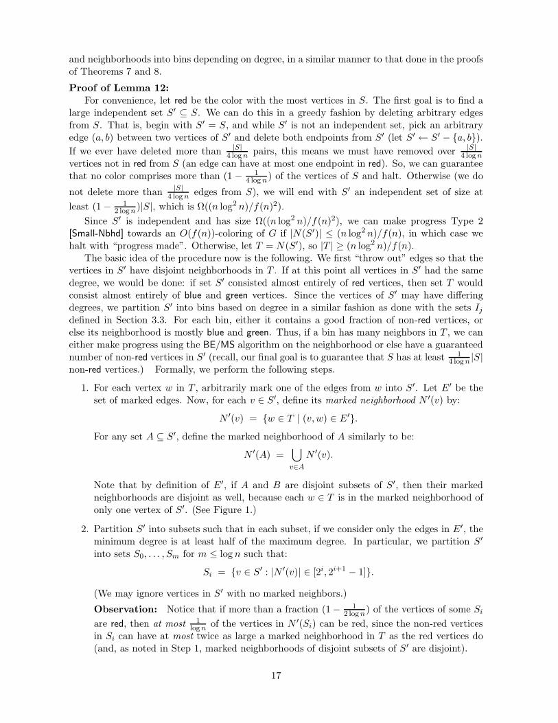
1. For each vertex w in T , arbitrarily mark one of the edges from w into S′. Let E′ be theset of marked edges. Now, for each v ∈ S′, define its marked neighborhood N ′(v) by:

N ′(v) = w ∈ T | (v,w) ∈ E′.For any set A ⊆ S′, define the marked neighborhood of A similarly to be:

N ′(A) =⋃

v∈A

N ′(v).

Note that by definition of E′, if A and B are disjoint subsets of S′, then their markedneighborhoods are disjoint as well, because each w ∈ T is in the marked neighborhood ofonly one vertex of S′. (See Figure 1.)

2. Partition S′ into subsets such that in each subset, if we consider only the edges in E′, theminimum degree is at least half of the maximum degree. In particular, we partition S′

into sets S0, . . . , Sm for m ≤ log n such that:

Si = v ∈ S′ : |N ′(v)| ∈ [2i, 2i+1 − 1].

(We may ignore vertices in S′ with no marked neighbors.)

Observation: Notice that if more than a fraction (1− 12 log n) of the vertices of some Si

are red, then at most 1log n of the vertices in N ′(Si) can be red, since the non-red vertices

in Si can have at most twice as large a marked neighborhood in T as the red vertices do(and, as noted in Step 1, marked neighborhoods of disjoint subsets of S′ are disjoint).

17

T

S′

E′

redblue and green

blue and green red

Figure 1: Vertices in S′ have disjoint marked neighborhoods. If the vertices had nearly identical“marked degree,” then a mostly red set S′ would imply a mostly blue and green set T .

3. Now, pick i0 such that |N ′(Si0)| is maximized; so |N ′(Si0)| ≥ ( 11+log n)|T | since there are at

most (1+log n) sets Si and their neighborhoods are disjoint. Note that i0 is not necessarilythe largest index, since lower index sets might have enough vertices to compensate forhaving fewer neighbors per vertex.

4. We now apply the BE/MS vertex-cover algorithm (or equivalently, algorithm Approx-IS inthe appendix) to the set N ′(Si0). If it finds an independent set of size Ω(n/f(n)), then wehave made progress Type 1 [Large-IS] and can halt with “progress made”.

The reason we apply the BE/MS vertex cover algorithm is that if more than a fraction(1 − 1

2 log n) of the vertices of Si0 are red, then by the observation in Step 2, N ′(Si0) has

at most a 1log n fraction of its vertices red, so N ′(Si0) has an independent set of at least

12(1− 1

log n) of its vertices, namely either N ′(Si0)∩blue or N ′(Si0)∩green, whichever is larger.

Thus, by Lemma 11, we find an independent set of size Ω(|N ′(Si0)|/ log n) = Ω(n/f(n))since we have assumed |T | ≥ (n log2 n)/f(n) and |N ′(Si0)| ≥ 1

1+log n |T |.So, if we do not make progress, we know it is not true that more than (1 − 1

2 log n) of thevertices of Si0 are red.

5. If we did not make progress in step 4, we know that at least 12 log n of the vertices in Si0

are blue or green. Now, let S′ ← S′ − Si0 and let T = N(S′).

If S′ has not been reduced to less than 1/3 its original size, then go back to Step 1. Noticethat in this case, we may still assume that |T | ≥ (n log2 n)/f(n) since S′ still has sizeΩ((n log2 n)/f(n)2).

If S′ is less than 1/3 its original size, then go on to Step 6.

6. If we reach this step, it means we have reduced S′ to less than a third of its original size,and have done so by removing from S′ sets containing at least a 1

2 log n fraction of blue and

green vertices. Since S′ originally had size at least (1 − 12 log n)|S|, this implies we must

18

have removed more than:

2

3

1

2 log n

[(

1− 1

2 log n

)

|S|]

≥ 1

4 log n|S|

blue and green vertices from S. So, we may halt with the guarantee asked for in thestatement of the lemma since set S could not possibly have contained more than (1 −

14 log n)|S| red vertices.

5.2 Making progress from dense regions

We will now use Lemma 12 to help take advantage of certain types of dense regions in 3-colorablegraphs. In particular, we consider the case of two sets of vertices S and T where S is 2-coloredunder some legal 3-coloring of G and the number of edges between S and T is large comparedwith the sizes of the two sets. This occurs when S is a subset of the neighborhood of a vertex(e.g., a set N(v) ∩ Ij) and T is some set Ni(S) for a large i (see Section 3.3).

Theorem 13 Given sets of vertices S and T in an n-vertex 3-colorable graph G, such that

1. S is 2-colored under some legal 3-coloring of G,

2. DT (S) = Ω(|S|(n log2 n)/f(n)2), and

3. [DT (S)]3 = Ω

(

[

|S|+ maxv∈S

dT (v)]

×[

|S||T |2(n log n)/f(n)2 + |T ||S|2n2/f(n)4]

)

,

then we can make progress towards an O(f(n))-coloring of G.

Before proving this theorem, let us first make sense of the condition on [DT (S)]3 by con-sidering a few examples. Suppose we wish to color with f(n) = n3/8 colors, the set S has size

n3/8, and each vertex v in S has degree n3/8 into T . Then, DT (S)|S| = n3/8, which is greater than

n1/4 log2 n (condition 2). The main condition (condition 3) reduces to:

n18/8 ≥ cn3/8[

|T |2n5/8 log n + |T |n10/8]

.

Ignoring logarithmic factors, the theorem assures us we make progress if |T | = O(n5/8). This isthe basic idea for the O(n3/8 log5/2 n)-coloring algorithm described later. For that applicationof this theorem, if T has Ω(n5/8) vertices, we will be able to find a large independent set insideT , and thus make progress of Type 1.

As another example, if we wished to color with n0.35 colors, S had size n0.35 and each vertexin S had degree n0.35 into T , then the main condition reduces to

n2.1 ≥ cn0.35[

|T |2n0.65 log n + |T |n1.3]

.

In this case, we only make progress if |T | = O(n0.45) (here the |T |n1.3 term is dominant).However, we do not know how to make use of forcing |T | = Ω(n0.45).

Proof of Theorem 13: For convenience, let blue and green be the two colors that appearin S, and let us define the following notation.

• Let Dtotal = DT (S) = DS(T ).

19

g

X

YT

S g'

blue green

bluegreen red

Figure 2: Vertex g and the sets X and Y . Also, green vertex g′ ∈ S (defined later) and theintersecting neighborhoods.

• Let davg = Dtotal/|S| be the average degree into T of vertices in S.

We want to keep track of those vertices of T that have a reasonably large degree into S, so wedefine a subset T ′ of T by:

• T ′ = w ∈ T | dS(w) ≥ 12

Dtotal|T | .

Since DS(T − T ′) < |T |[

12

Dtotal|T |

]

, we have DS(T ′) ≥ 12Dtotal, or equivalently,

DT ′(S) ≥ Dtotal/2. (13)

We also want to look at those vertices in S that have reasonably large degree into T ′, so define:

• S′ = v ∈ S | dT ′(v) ≥ 12

DT ′(S)|S| .

Since DT ′(S − S′) < |S|[

12

DT ′ (S)|S|

]

, we have: DT ′(S′) ≥ 12DT ′(S), which by equation 13 implies:

DT ′(S′) ≥ Dtotal/4. (14)

Also, by definition of S′ and equation (13), if v ∈ S′ then dT ′(v) ≥ 14

Dtotal|S| or equivalently,

dT ′(v) ≥ 14davg for all v ∈ S′. (15)

Since we are given (condition 2) that davg = Ω((n log2 n)/f(n)2), this implies that all v ∈ S′

have dT (v) ≥ dT ′(v) = Ω((n log2 n)/f(n)2). Thus, by Lemma 12 (applied to the sets N(v)∩ T ),we can guarantee that each vertex v ∈ S′ has at least a fraction 1

4 log n of its edges into T enteringinto non-red vertices.

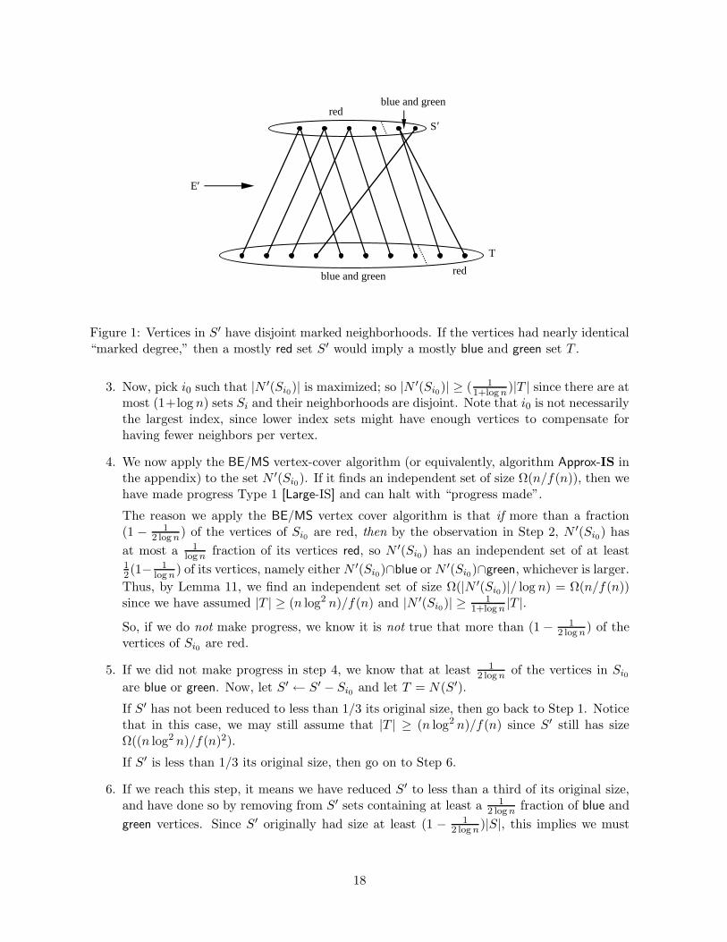
So, for some non-red color, say green without loss of generality, at least DT (S′)/(8 log n)edges from S′ enter into green vertices of T . This implies that some green vertex g ∈ T hasdegree at least DT (S′)/(8|T | log n) into S′. Now, define (see Figure 2):

• X = N(g) ∩ S′.

20

• Y = N(X) ∩ T ′.

So, we have:

|X| ≥ 18DT (S′)/(|T | log n)

≥ 132Dtotal/(|T | log n)

= Ω((

|S||T |

) (

davg

log n

))

. (16)

Note that set X consists entirely of blue vertices, and since Y is in the neighborhood of a blueset, Y contains only red and green vertices. We want to show that Y is large, because we willlater intersect Y with a red and blue set to get a large monochromatic (red) set, which will allowus to make progress. We show that Y must be large as follows.

By Theorem 3 we may assume that no two vertices of X share more than n/f(n)2 neighbors

in T ′. Now suppose that |X| < f(n)2

n (18davg). In this case, each vertex v ∈ X can share at most

|X|(n/f(n)2) < 18davg neighbors with other vertices in X. This implies, by equation (15), that

v must have at least 18davg neighbors in T ′ not shared with any other vertices of X. So, set Y

must have size at least Ω(|X|davg).

If |X| ≥ f(n)2

n (18davg), then if we only consider the first f(n)2

n (18davg) of the vertices of X, we

still get that |Y | = Ω(f(n)2

n (davg)2). So, whichever case occurs, we have:

|Y | = Ω(

min

|X|davg,f(n)2

n (davg)2)

. (17)

By definition, Y is a subset of T ′ and vertices of T ′ all have a high degree into S. So, we canlower bound the degree of Y into S by:

DS(Y ) ≥(

12

Dtotal|T |

)

|Y |

= 12|S||T |davg|Y |

= Ω(

min

|X| |S||T |(davg)2, f(n)2

n (davg)3 |S||T |

)

(by equation 17)

= Ω

(

min

[

|S||T |

]2(davg)

3/ log n, f(n)2

n (davg)3 |S||T |

)

. (by equation 16) (18)

Now we apply condition 3 in the statement of the theorem. The condition (dividing both sides by

|S|3) states that (davg)3 =

[

|S|+ maxv∈S dT (v)]

·Ω(

|T |2

|S|2n

f(n)2 log n + |T ||S|

n2

f(n)4

)

. So, this implies

both that:[

|S||T |

]2(davg)

3/ log n =[

|S|+ maxv∈S

dT (v)]

· Ω(

nf(n)2

)

(19)

and

f(n)2

n (davg)3[

|S||T |

]

=[

|S|+ maxv∈S

dT (v)]

· Ω(

nf(n)2

)

. (20)

Thus, combining both equations (19) and (20) with equation (18), we get:

DS(Y ) = Ω

(

nf(n)2

[

|S|+ maxv∈S

dT (v)]

)

. (21)

It now must be that one of the following two cases occurs. The first case is that there issome green vertex g′ ∈ S in the neighborhood of more than 1

2DS(Y )/|S| vertices of Y . In this

21

case, according to equation (21), it must be that Dg′(Y ) = Ω(n/f(n)2). So, N(g′)∩Y is a setof Ω(n/f(n)2) vertices, all of which are red since N(g′) ⊆ blue ∪ red and Y ⊆ red ∪ green; seeFigure 2. Thus, we can make progress on this monochromatic set using Corollary 4.

The other possibility is that no green vertex in S is in the neighborhood of more than12DS(Y )/|S| vertices of Y . In this case, the set of all vertices in S hit by more than 1

2DS(Y )/|S|edges from Y is all blue. Define Z to be that set; that is:

• Z = v ∈ S | dY (v) > 12DS(Y )/|S|.

Clearly, the number of edges between vertices of Y and vertices in (S−Z) is at most |S|(12DS(Y )/|S|) =

12DS(Y ). So, DZ(Y ) ≥ 1

2DS(Y ). Thus, we can bound the size of Z by:

|Z| ≥ 12DS(Y )/max

v∈SdY (v)

≥ 12DS(Y )/max

v∈SdT (v)

which by equation (21) implies:|Z| = Ω(n/f(n)2).

Since Z is monochromatic (blue) we can again use Corollary 4 to make progress. So, whicheverof the two cases occurs, we have made progress towards an O(f(n))-coloring.

The final algorithm for making progress given our sets S and T is as follows:

Algorithm Dense-Region-Progress:

Given: Sets S and T satisfying the conditions of Theorem 13 in some graph G.

Output: Progress towards an O(f(n))-coloring of G.

1. Run the algorithm of Lemma 12 on N(v)∩T for all v ∈ S. If any runs make progresstowards an O(f(n))-coloring, then halt. Otherwise, we know there are many edgesfrom S into red, blue, and green vertices of T under any legal 3-coloring of G.

2. If for some pair of vertices u, v ∈ S, we have |N(u) ∩ N(v)| ≥ n/f(n)2, then useTheorem 3 to make progress.

3. Otherwise, for each vertex v ∈ T ,

(a) let Y = N(N(v) ∩ S) ∩ T and let Z = w ∈ S : dY (w) ≥ n/f(n)2.(Note that we do not actually need to use the sets S′ and T ′; they were justconvenient for the analysis.)

(b) Run the algorithm of Corollary 4 on Z.

(c) For each w ∈ Z, run the algorithm of Corollary 4 on Y ∩N(w).

The above proof guarantees that this algorithm makes progress.

5.3 The coloring algorithm

We now combine algorithms First-Approx and Dense-Region-Progress to get an improved algo-rithm guaranteed to O(n3/8)-color any n-vertex 3-colorable graph.

Algorithm Improved-Approx:

Given: G = (V,E), a 3-colorable graph on n vertices. Let f(n) = n3/8(log n)5/2.

Output: Progress towards an O(f(n))-coloring of G.

22

1. For each vertex v, if d(v) < f(n), make progress Type 2 [Small-Nbhd].

2. Otherwise, for each vertex v, for each i, j ∈ 0, 1, . . . , 5(log n)2:(a) Let S = N(v) ∩ Ij .

(b) Let T = Ni(S).

(c) If |T | ≥ n5/8/(log n)3/2, run the BE/MS Vertex-Cover approximation algorithm.If we find an independent set of size at least n/f(n), we have made progress Type1 [Large-IS].

(d) If S and T satisfy the conditions of Theorem 13, then make progress using Algo-rithm Dense-Region-Progress.

Theorem 14 Algorithm Improved-Approx will make progress towards an O(n3/8(log n)5/2)-coloringof any n-vertex 3-colorable graph.

Proof: Assume Algorithm Improved-Approx does not make progress in Step 1. So, we know thatthe minimum degree d ≥ f(n) = n3/8(log n)5/2. As in Section 4, let R = red be the color classwith D(red) = max (D(red), D(blue), D(green)).

We now apply some of the facts proven in Section 4.3.2. Theorem 7 guarantees us that forsome vertex v ∈ R and some index j, the set S = N(v) ∩ Ij in Step 2(a) has the property that:

|S| ≥ δ2f(n)/ log1+δ n, and (22)

DR(S) ≥ 12(1− 3δ)D(S), (23)

where δ = 15 log n . Note that for the given value of f , equation (22) and the definition of δ imply

that:

|S| = Ω(n3/8/(log n)3/2). (24)

Theorem 8 (using λ′ = 12(1 − 3δ)) shows that for some index i, the set T = Ni(S) of step 2(b)

has the property that:

DT∩R(S) ≥ δDR(S)/ log1+δ n, and (25)

|T ∩R|/|T | ≥ 12(1− 2δ)(1 − 3δ). (26)

Let us now, for the rest of the proof, fix two such sets S and T satisfying equations (22) through(26). We now show that these equations and the definitions of S and T will ensure success ofthe algorithm.

Suppose first that |T | ≥ n5/8/(log n)3/2. By equation 26 above, set T contains an independentset (T∩R) of at least a fraction 1

2 (1− 1log n) of its vertices (using δ = 1

5 log n). So by Lemma 11, the

BE/MS vertex-cover algorithm finds an independent set of size Ω(

n5/8/(log n)5/2)

= Ω(n/f(n))

so we make progress Type 1 [Large-IS] in Step 2(c).On the other hand, if |T | < n5/8/(log n)3/2, then we just need to show that S and T satisfy

the conditions of Theorem 13. Clearly, S is 2-colored under any legal 3-coloring of G sinceS ⊆ N(v), so Condition 1 is satisfied. For f(n) = n3/8(log n)5/2, Condition 2 reduces to

DT (S)/|S| = Ω(

n1/4/(log n)3)

, which is found to be easily met using equations (23) and (25)

as follows.

DT (S) ≥ DT∩R(S) = Ω(

D(S)/(log n)3)

(27)

= Ω(d|S|/(log n)3). (28)

23

So,

DT (S)/|S| ≥ Ω(n3/8/(log n)1/2) (29)

= Ω(n1/4/(log n)3). (30)

The last task is to show that Condition 3 is satisfied, which for the given value of f , reducesto the requirement that

[DT (S)]3 = Ω

(

[

|S|+ maxv∈S

dt(v)]

·[

|S| |T |2 n1/4

(log n)4+ |T | |S|2 n1/2

(log n)10

]

)

. (31)

To show that this requirement holds, we upper bound the quantities |S|, |T |, and maxv∈S dT (v).From equation (29), we have

|S| = O(

(log n)1/2DT (S)/n3/8)

. (32)

Next, our very condition for this case was that:

|T | = O(

n5/8/(log n)3/2)

. (33)

Finally, since S ⊆ Ij so all vertices of S have nearly the same degree (though not necessarilythe same degree into T ), we can bound maxv∈S dT (v) as follows:

maxv∈S

dT (v) = O(D(S)/|S|)

= O(DT (S)(log n)3/|S|) (using equation 27)

= O(

DT (S)(log n)3(log n)3/2/n3/8)

(using equation 24)

= O(

DT (S)(log n)9/2/n3/8)

. (34)

The three equations (32), (33), and (34) allow us to reduce requirement (31) to the conditionthat:

[DT (S)]3 = Ω

(

[

(log n)9/2 DT (S)

n3/8

]

·[

DT (S)n9/8

(log n)13/2+ DT (S)2

n3/8

(log n)21/2

]

)

= [DT (S)]2 · Ω(

n3/4

(log n)2+

DT (S)

(log n)6

)

. (35)

Equivalently, we just have the requirement that DT (S) = Ω(n3/4/(log n)2 + DT (S)/(log n)6).

Clearly, DT (S) = Ω(DT (S)/(log n)6) so we simply need DT (S) = Ω(

n3/4/(log n)2)

. We are

now done, because combining equations (29) and (24) yields:

DT (S) = Ω(

|S| n3/8/(log n)1/2)

= Ω(

n3/4/(log n)2)

.

Thus, Step 2(d) of Algorithm Improved-Approx makes progress.

24

k = 3 4 5 6 7 general

Wigderson [Wig83] n1/2 n2/3 n3/4 n4/5 n5/6 n1− 1k−1

n0.5 n0.667 n0.75 n0.8 n0.833

base: k = 3 n3/8 n8/13 n13/18 n18/23 n23/28 n1− 1

k−7/5

n0.375 n0.615 n0.722 n0.783 n0.821

base: k = 4 — n3/5 n5/7 n7/9 n9/11 n1− 1

k−3/2

— n0.6 n0.714 n0.778 n0.818

best we have n3/8 n3/5 n91131 n

105137 n

53016581

n0.375 n0.6 n0.695 n0.766 n0.806

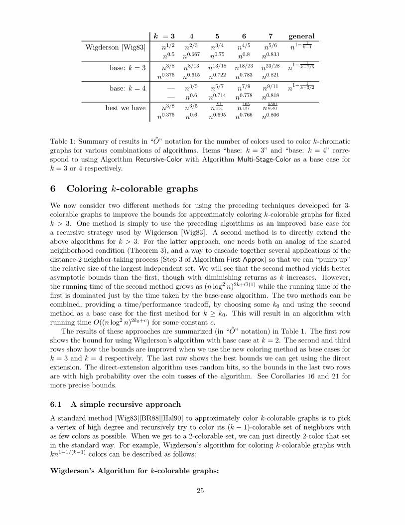
Table 1: Summary of results in “O” notation for the number of colors used to color k-chromaticgraphs for various combinations of algorithms. Items “base: k = 3” and “base: k = 4” corre-spond to using Algorithm Recursive-Color with Algorithm Multi-Stage-Color as a base case fork = 3 or 4 respectively.

6 Coloring k-colorable graphs

We now consider two different methods for using the preceding techniques developed for 3-colorable graphs to improve the bounds for approximately coloring k-colorable graphs for fixedk > 3. One method is simply to use the preceding algorithms as an improved base case fora recursive strategy used by Wigderson [Wig83]. A second method is to directly extend theabove algorithms for k > 3. For the latter approach, one needs both an analog of the sharedneighborhood condition (Theorem 3), and a way to cascade together several applications of thedistance-2 neighbor-taking process (Step 3 of Algorithm First-Approx) so that we can “pump up”the relative size of the largest independent set. We will see that the second method yields betterasymptotic bounds than the first, though with diminishing returns as k increases. However,the running time of the second method grows as (n log2 n)2k+O(1) while the running time of thefirst is dominated just by the time taken by the base-case algorithm. The two methods can becombined, providing a time/performance tradeoff, by choosing some k0 and using the secondmethod as a base case for the first method for k ≥ k0. This will result in an algorithm withrunning time O((n log2 n)2k0+c) for some constant c.

The results of these approaches are summarized (in “O” notation) in Table 1. The first rowshows the bound for using Wigderson’s algorithm with base case at k = 2. The second and thirdrows show how the bounds are improved when we use the new coloring method as base cases fork = 3 and k = 4 respectively. The last row shows the best bounds we can get using the directextension. The direct-extension algorithm uses random bits, so the bounds in the last two rowsare with high probability over the coin tosses of the algorithm. See Corollaries 16 and 21 formore precise bounds.

6.1 A simple recursive approach

A standard method [Wig83][BR88][Hal90] to approximately color k-colorable graphs is to picka vertex of high degree and recursively try to color its (k − 1)-colorable set of neighbors withas few colors as possible. When we get to a 2-colorable set, we can just directly 2-color that setin the standard way. For example, Wigderson’s algorithm for coloring k-colorable graphs withkn1−1/(k−1) colors can be described as follows:

Wigderson’s Algorithm for k-colorable graphs:

25

Given: A k-colorable graph G on n vertices.

Output: A coloring with at most kn1−1/(k−1) colors.

1. If there exists a vertex v with at least n1−1/(k−1) neighbors, then color the neighbor-

hood recursively with (k− 1)(

n1−1/(k−1))1− 1

k−2= (k− 1)

(

nk−2k−1

)k−3k−2

= (k− 1)nk−3k−1

colors. Then remove those nodes from the graph and the colors from the palette.

Note that this step can be executed at most n1/(k−1) times, resulting in a total of

(k − 1)nk−3k−1

+ 1k−1 = (k − 1)n1−1/(k−1) colors used in this step.

2. Otherwise, greedily color the graph left with n1−1/(k−1) colors.

So, the total number of colors used in both steps together is

kn1−1/(k−1).

(Note that for the base case of k = 2, we have 2 = 2n1−1/(2−1).)

The algorithms presented in the previous sections allow one to stop at k = 3 as a basecase instead of k = 2 in this type of procedure and thus use fewer colors. More generally, wecan describe when a bound achieved for coloring graphs of chromatic number k0 will improvethe performance of this kind of recursive procedure for graphs of higher chromatic number. Inparticular, suppose we have an algorithm A to color any n-vertex k0-colorable graph with O(nα)colors. Then, the important quantity for this approach, which we call the recursive performancer(A) of the algorithm, is:

r(A) = k0 −1

1− α. (36)

If an algorithm has a higher value of r, then the bounds achieved by using that as a base casefor k > k0 will be improved. Specifically, the recursive algorithm will color k-colorable graphs

for k ≥ k0 with O(

n1−1/(k−r(A)))

colors. So, for example, using the fact that we can 2-color

2-colorable graphs (k0 = 2, α = 0), we find r = 1 and the bound is O(

n1−1/(k−1))

. Using

the improved bounds for coloring 3-colorable graphs in Section 5 (k0 = 3, α = 3/8), we getr = 3− 1

5/8 = 7/5, so the improved bound for k ≥ 3 is:

O

(

n1− 1

k−7/5

)

colors. (37)

Later, in Section 6.2, we will see how to color 4-colorable graphs with O(n3/5) colors, so we get

r = 4− 12/5 = 3/2. Thus, for k ≥ 4, we can color with O(n

1− 1k−3/2 ) colors.

The following theorem more precisely describes the bounds achieved by the recursive ap-proach.

Theorem 15 Given an algorithm A to color any m-vertex k0-colorable graph with cmα logβ mcolors, then algorithm Recursive-Color(A) below can color any n-vertex k-colorable graph (k ≥ k0)with at most:

Ck(n) = [c + (k − k0)]n1−1/(k−r) (log n)β

[

k0−r

k−r

]

(38)

colors, where r = r(A) = k0 − 11−α .

26

Using Theorem 15 and the bounds achieved by algorithm Improved-Approx, (k0 = 3, α =3/8, β = 5/2),we can restate formula (37) more precisely in the following corollary.

Corollary 16 Algorithm Recursive-Color(Improved-Approx) colors any n-vertex k-colorable graph(k ≥ 3) with at most

O

(

n1− 1

k−7/5 (log n)4

k−7/5

)

colors.

The recursive algorithm to achieve these bounds is described below.

Algorithm Recursive-Color: (Variant on Wigderson’s algorithm)

Given: An n-vertex k-colorable graph G and an algorithm A to color any m-vertex k0-colorable graph with at most Ck0(m) = cmα logβ m colors (k0 ≤ k).

Output: A Ck(n)-coloring of G, for Ck(n) as defined in equation (38).

1. Let r = k0 − 11−α .

2. Let f(n, k) = n1−1/(k−r)(log n)βk0−r

k−r .

3. While there exists a vertex with at least f(n, k) neighbors, select f(n, k) of its neigh-bors and color them with Ck−1(f(n, k)) colors. Remove those nodes from the graphand the colors from the palette.

Note that we can execute this step at most n/f(n, k) times.

4. Otherwise, greedily color the graph with f(n, k) colors.

Proof of Theorem 15: Let A be an algorithm that colors any m-vertex k0-colorable graphwith cmα logβ m colors and let r = r(A). We will use Ck(n) to denote the coloring boundachieved on n-vertex k-colorable graphs. First, formula (38) in the statement of the theoremholds for the base case of k = k0 since for k = k0, we have:

Ck0(n) = cn1− 1

1/(1−α) (log n)β·1

= cnα logβ n.

Let ck = c + (k − k0) and let f(n, k) = nk−r−1

k−r (log n)βk0−rk−r as in Algorithm Recursive-Color.

So, assuming the bounds of Theorem 15 inductively for k′ < k, we need to show that Ck(n) ≤ckf(n, k).

Since we can loop in step 3 of Algorithm Recursive-Color at most n/f(n, k) times, this resultsin the recurrence:

Ck(n) ≤ Ck−1 (f(n, k)) [n/f(n, k)] + f(n, k).

So, substituting in the bounds of Theorem 15 inductively, we have:

Ck(n) ≤[

ck−1[f(n, k)]1−1/(k−r−1)[log f(n, k)]β(

k0−r

k−r−1

)

]

[

nf(n,k)

]

+ f(n, k)

< ck−1[f(n, k)]1−1/(k−r−1)[log n]β(

k0−rk−r−1

)

[

nf(n,k)

]

+ f(n, k)

= ck−1n[f(n, k)]−1/(k−r−1)[log n]β(

k0−r

k−r−1

)

+ f(n, k)

27

= ck−1n

(

nk−r−1

k−r

)−1

k−r−1(

[log n]βk0−rk−r

)−1

k−r−1

[log n]β(

k0−r

k−r−1

)

+ f(n, k)

= ck−1n1− 1

k−r [log n]β(

k0−rk−r

)

+ f(n, k)

= ck−1f(n, k) + f(n, k)

= ckf(n, k).

6.2 Directly extending the k = 3 algorithm

6.2.1 Intuition

In this section, we describe how the methods of Algorithm First-Approx of Section 4 can be ap-plied directly to graphs of higher chromatic number, yielding improved coloring bounds forsuch graphs. Unfortunately, we do not know a way to extend the approach of AlgorithmImproved-Approx in a similar way, though it can still provide a useful “base case”.

The main idea of Algorithm First-Approx was to look at large subsets of the distance-2neighbors of vertices in a 3-colorable graph: in particular, the sets Ni(N(v)∩ Ij) for each vertexv and each pair of indices i, j. The “well-distributed” property proved in Theorems 7 and 8ensures that one such set will be nearly half red under some legal 3-coloring of the graph, andthe expansion property of Theorem 3 ensures the set is large as well.

While the expansion property depended heavily on the graph being 3-colorable, the theoremsforcing good distribution require only that the given graph have an independent set of large totaldegree (see Section 4.3.2). In particular, they simply require that there exist a large independentset R such that DR(V −R) ≥ λD(V −R) for some constant λ and that the graph have sufficientlylarge minimum degree. So, we could conceivably make progress on graphs of a higher chromaticnumber than 3 by cascading several applications of the distance-2 neighbor-taking stage in thefollowing way.

Suppose, say, G is a 5-colorable graph and we wish to color G with f(n) colors. Then,we know there exists an independent set R such that DR(V − R) ≥ 1

4D(V − R) and we canestablish a minimum degree of f(n). If we could guarantee that no two vertices shared too manyneighbors, we could look at the sets Tv,i,j and be assured that one will be large and have anindependent set R′ = R ∩ Tv,i,j such that |R′| ≈ 1

4 |Tv,i,j | using Theorems 7 and 8. Let us nowfocus on the subgraph G′ induced by Tv,i,j , and let V ′ = Tv,i,j . Suppose we could in additionsomehow ensure that within G′, the vertices of R′ had about the same average degree as theother vertices of V ′. Then we would have D(R′) ≈ 1

4D(V ′), which would imply that:

DR′(V ′ −R′) ≈ 13D(V ′ −R′), (39)

since DR′(V ′ −R′) = D(R′) and D(R′) ≈ 14D(V ′) = 1

4(D(V ′ −R′) + D(R′)), where we are nowcounting degrees only within G′.

Now, if we re-establish a minimum degree without destroying (39) above, we could then re-apply the distance-2 neighbor-taking process within G′ to get a set V ′′ containing an independentset R′′ such that |R′′| ≈ 1

3 |V ′′|. If again we could ensure that D(R′′) ≈ 13D(V ′′) within the new

graph G′′, we would get:DR′′(V ′′ −R′′) ≈ 1

2D(V ′′ −R′′).

Thus, one final application of examining the sets Tv,i,j within G′′ will yield some set on whichthe BE/MS vertex-cover algorithm makes progress.

28

So, the two main ingredients needed to make this procedure go through are (1) how to ensurethat no two vertices share too many neighbors in common, and (2) how to get from |R′| ≈ λ|V ′|to D(R′) ≈ λD(V ′). These problems are solved in the following sections.

6.2.2 The bootstrapping algorithm

We now describe procedures that allow us to “bootstrap” applications of Algorithm First-Approxto graphs of higher chromatic number. The resulting algorithm Multi-Stage-Color will color anyn-vertex k-colorable graph with:

• fk(n) = O(nα(k) logβ(k) n) colors,

where α(k) will be defined inductively in k, and β(k) is a nondecreasing function such thatβ(k) ≤ 5.5. The exponent β of the logarithm in fact approaches 5.5 as k →∞. Because αis the critical value and the log factors are low-order terms, for purposes of simpler analysiswe will not attempt to get tight bounds and assume β is fixed at 5.5 for all k > 3.

For base cases, α(2) = 0 and α(3) = 3/8 using algorithm Improved-Approx. The recursive formulafor α(k) for k > 3 is:

1

1− α(k)= 2− 1

2k−2+

1

1− α(k − 2)

(

1− 1

2k−2

)

. (40)

We will examine this formula in more detail later, but we just note here that α is non-decreasingin k.

We need in this section to redefine the value δ to depend on the chromatic number k of thegraph G we wish to color. In particular, we shall use:

• δ = δ(k) =1

4k log n.

The sets Ij and Ni(v) used in Section 4 now depend on this new quantity.As mentioned previously, the theorems of Section 4.3.2 forcing good distribution do not

require that the graph be 3-colorable, only that there exist a large independent set R such thatDR(V −R) ≥ λD(V −R) for some constant λ and that the graph have sufficiently large minimumdegree. Let us, in fact, repeat Corollary 9 here, removing all mention of the chromatic numberof the graph. (The fact that the graph was 3-colorable was used only in showing that λ ≥ 1/2.)

Corollary 17 (Variant of Corollary 9) Suppose G = (V,E) is an n-vertex graph such that(1) no two vertices share more than s neighbors, (2) G has minimum degree dmin ≥ (10 log n)/δ2],and (3) G contains an independent set R such that DR(V −R) ≥ λD(V −R) for some constantλ ∈ [0, 1]. Then, for any δ = 1

Θ(log n) , for some v ∈ V and some i, j ∈ [0, . . . , log1+δ n], the set

Tv,i,j = Ni(N(v) ∩ Ij)

has size at least Ω(

(dmin)2/(s log7 n))

and the property that |Tv,i,j ∩R| ≥ λ(1− 5δ)|Tv,i,j |.

We now present a new method to ensure that no two vertices share too many neighbors.

Theorem 18 Given an n-vertex k-colorable graph G containing two vertices that share at least

n1−α(k)

1−α(k−2) neighbors and an algorithm A to color any m-vertex (k − 2)-colorable graph withfk−2(m) colors, Algorithm Sharing-Progress below will make progress towards an fk(n)-coloringof G.

29

Algorithm Sharing-Progress:

Given: (1) An n-vertex k-colorable graph G containing two vertices that share at least

n1−α(k)

1−α(k−2) neighbors, and (2) an algorithm A to color any m-vertex (k− 2)-colorable graphwith fk−2(m) colors.

Output: Progress towards an fk(n) coloring of G.

1. Let S = N(x) ∩ N(y) where x and y share at least n1−α(k)

1−α(k−2) neighbors, and let GS

be the subgraph induced by set S.

2. Run algorithm A on GS . Note that if GS is (k − 2)-colorable, then A will color GS

with at most:

fk−2(|S|) = O(|S|α(k−2)(log |S|)β(k−2))

≤ O(|S|α(k−2)(log n)β(k)) colors,

(using |S| ≤ n and β non-decreasing). Thus, Algorithm A will find an independentset of size at least:

Ω( |S|1−α(k−2)

(log n)β(k)

)

= Ω( n1−α(k)

(log n)β(k)

)

(for the given choice of |S|)

= Ω(n/fk(n)).

Thus, if GS is (k − 2)-colorable, then we have made progress of Type 1 [Large-IS].

3. If we did not make progress in Step 2, it must be that GS was not (k − 2)-colorable.The only way this could be is if x and y must be the same color under any legalk-coloring of G. So, we can merge vertices x and y and make progress of Type 3[Same-Color].

The argument given in Algorithm Sharing-Progress proves Theorem 18.

We now use Algorithm Sharing-Progress in a procedure that allows us to “bootstrap” appli-cations of Step 3 of Algorithm First-Approx.

Algorithm Bootstrap:

Given: (1) Values α ∈ [0, 1], β > 0 and δ = 1Θ(log n) , and (2) An m-vertex subgraph

H (m ≫ 1/δ2) of an n-vertex graph G such that H contains an independent set R with|R| ≥ λ|V (H)| for some constant λ > 0.

Output: Either: (1) progress towards an O(nα logβ n)-coloring of G, or else (2) at mostm/2 subgraphs G0, G1, . . . , Gm/2−1 of H such that with high probability at least one

Gi has both a minimum degree of (δ2 mn )nα logβ n and considering only edges within Gi,

D(R ∩ V (Gi)) ≥ (λ− 2δ)D(V (Gi)).

1. Let G0 = (V0, E0) = H. Inductively create graph Gi = (Vi, Ei) from graph Gi−1

for i = 1, 2, . . . ,m/2 − 1 by selecting an edge at random in Ei−1 and deleting bothendpoints. So, |Vi| = |Vi−1 − 2|.

30

2. For each Gi with at least δm vertices, while Gi contains a vertex with degree lessthan δ2mnα−1 logβ n: delete from Gi the vertex of minimum degree and all incidentedges.

Suppose we have removed more than δ2m vertices from any Gi. Since within the setWi of vertices deleted from Gi, the degree of each vertex can be at most δ2mnα−1 logβ n,we can greedily find an independent set inside Wi of size at least:

δ2m

δ2mnα−1 logβ n= n/(nα logβ n).

So, we make progress Type 1 [Large-IS] towards an O(nα logβ n)-coloring of G.

3. If we did not make progress in Step 2, then output the graphs Gi for i = 0, 1, . . . ,m/2−1.

Theorem 19 [Algorithm Bootstrap works as guaranteed] Given an m-vertex subgraph H (m≫1/δ2) of an n-vertex graph G such that H contains an independent set R with |R| ≥ λ|V (H)| forsome constant λ. Then, either (1) Algorithm Bootstrap makes progress towards an O(nα logβ n)-coloring of G in Step 2, or else (2) with high probability, one of the subgraphs Gi = (Vi, Ei) hasboth a minimum degree of δ2mnα−1 logβ n and within the subgraph, D(R∩ Vi) ≥ (λ− 2δ)D(Vi).

Proof: Let us consider the graphs Gi created after Step 1 of Algorithm Bootstrap, butbefore deleting vertices in Step 2. Let Ri = Vi ∩ R and let N = m(1 − δ)/2; note that set VN

contains δm vertices. We show now that with high probability, for some index i ≤ N , we haveD(Ri) ≥ (λ − δ)D(Vi). The idea of the argument is that since we are removing vertices with aprobability proportional to their degree, if D(Ri) < (λ− δ)D(Vi) for all such i, then we wouldremove many fewer vertices from R than from V − R. In fact, with high probability we wouldremove so many fewer that once we reach graph GN , the set RN would be larger than than VN ,a clear contradiction.

For each i ≤ N , let Ai be the event that in creating Gi+1 from Gi, we delete an edge withan endpoint in Ri. Since the number of edges in Ei with an endpoint in Ri is exactly D(Ri)(because Ri is an independent set), we have:

Pr[Ai] = D(Ri)/|Ei|= 2D(Ri)/D(Vi). (41)

Suppose for some index i ≤ N we have D(Ri) ≤ (λ − δ)D(Vi). Then, the probability event Ai

occurs is at most 2(λ− δ).Let p = 2(λ − δ) and assume for contradiction that D(Ri) < (λ− δ)D(Vi) for every i ≤ N .

So, for each i ≤ N , the probability that the ith edge removed from G has an endpoint in Ris less than p. Since we remove N edges to create GN and each time we remove an edge theprobability it has an endpoint in R is less than p, by Chernoff bounds [AV79] the probabilitywe remove more than pN(1 + δ) vertices from R is at most e−δ2Ω(pN). Since pN = Ω(m) andwe assume m ≫ 1/δ2 in the statement of the theorem, the probability we remove more thanpN(1 + δ) vertices from R is o(1). Thus, with high probability:

|RN | ≥ λm− pN(1 + δ)

= λm− 2(λ− δ)[m(1 − δ)/2](1 + δ)

= m[λ− (λ− δ)(1 − δ2)]

= δm + mδ2(λ− δ)

> δm. (since λ > δ)

31

So, with high probability, |RN | > |VN |, a contradiction. Thus, with high probability our as-sumption that D(Ri) < (λ− δ)D(Vi) for every i ≤ N is incorrect; that is, for some Vi of size atleast δm, we have D(Ri) ≥ (λ− δ)D(Vi).

Now, let i be such that |Vi| > δm and D(Ri) ≥ (λ − δ)D(Vi) before Step 2 of AlgorithmBootstrap. In Step 2, if at most δ2m vertices are removed, then we remove at most a fractionδ of the vertices of Vi in order to establish the desired minimum degree. Since we are alwaysremoving the vertex of least degree, we remove at most δD(Vi) from the total degree sum of thesubgraph. Even if, at worst, all the vertices removed were from the set Ri, we still have in thegraph remaining that:

D(Ri) ≥ (λ− 2δ)D(Vi),

as claimed.

Given Theorem 19, we have an improved approximation algorithm for coloring graphs ofchromatic number k > 3 as follows. We first apply algorithm Sharing-Progress; we then run thedistance-2 neighbor-taking stage of Algorithm First-Approx k−2 times, using Algorithm Bootstrapto “clean up” the graph in between applications; and finally, we use the BE/MS vertex-coveralgorithm. The formal algorithm to color any k-colorable graph with O(nα(k) logβ(k) n) colors isgiven below. For simplicity, we have separated out the distance-2-neighbor/bootstrap step intoa separate procedure.

Algorithm Multi-Stage-Color:

Given: An n-vertex k-colorable graph G.

Output: Progress towards an O(nα logβ n)-coloring of G for α = α(k) as defined by therecursion in equation (40), and β at most 5.5.

Let f(n) = nα logβ n.

1. [Base case] If k = 2 then just color G with 2 colors. If k = 3, then run AlgorithmImproved-Approx on G.

2. [Minimum degree] For each vertex v, if d(v) < f(n), make progress Type 2.

3. [Minimum sharing of neighbors] For each pair of vertices u, v, if |N(u) ∩ N(v)| ≥n

1−α(k)1−α(k−2) , then make progress using Algorithm Sharing-Progress. Note that Algorithm

Sharing-Progress will use Algorithm Multi-Stage-Color recursively on (k− 2)-colorablegraphs.

4. [Initial distance-2 neighbors] For each vertex v and each pair i, j ∈ [0, . . . , log1+δ n],let Gv,i,j be the subgraph induced by the set Ni(N(v) ∩ Ij).

5. [Additional neighbor-taking stages] For each graph Gv,i,j , run ProcedureIterate-neighbors below on input (n, k,Gv,i,j , k − 3).

If the algorithm makes progress on any of the inputs given, then halt with success.Otherwise, let G1, . . . , Gq be all the graphs returned by Iterate-neighbors, for q =O([(log1+δ n)2k−4n2k−5).

6. [Vertex-Cover approximation] Run the BE/MS vertex-cover algorithm on the graphsG1, . . . , Gq.

Procedure Iterate-neighbors: (n, k,G′, iter)

Given: Values n and k. An m-vertex subgraph G′ of some n-vertex graph G, and anumber of iterations iter.

32

Output: O([m2(log1+δ m)2]iter ) subgraphs of G′ or else progress towards an

O(nα(k) logβ(k) n)-coloring of G.

P1. If iter = 0, then return G′.

P2. If iter ≥ 1, then run Algorithm Bootstrap on G′ and values α = α(k), β = β(k), andδ = δ(k).

P3. If Algorithm Bootstrap returns progress towards an O(nα(k) logβ(k) n)-coloring of G,then halt with success. Otherwise, let H0, . . . ,Hm

2−1 be the subgraphs returned.

P4. Now, for each Hl, (0 ≤ l ≤ m2 − 1) for each vertex v in Hl and each index i, j ∈

[0, . . . , log1+δ m]:

(note: there are at most m2(log1+δ m)2 different 4-tuples (l, v, i, j))

(a) Let Gl,v,i,j be the subgraph of Hl induced by Ni(N(v)∩Ij), where neighborhoodsare taken within Hl.

(b) Run: Iterate-neighbors(n, k,Gl,v,i,j , iter − 1).

Theorem 20 Algorithm Multi-Stage-Color, given any n-vertex k-colorable graph, makes progresstowards a coloring with O(nα(k)(log n)5.5) colors, for α(k) as defined in equation (40).

Before proving Theorem 20, let us examine the claimed performance more closely. Letγ(k) = 1

1−α(k) . So, equation (40) can be written as:

γ(k) = 2− 1

2k−2+ γ(k − 2)

(

1− 1

2k−2

)

. (42)

One can see from this equation immediately that γ(k) < 2 + γ(k − 2); that is, if we increasek by 2, then γ increases by less than 2. We can compare this with the simpler approach fromSection 6.1. Algorithm Recursive-Color given there colors k-colorable graphs with O(nα′(k)) colorsfor α′(k) = 1 − 1

k−r for some constant r. Thus, the quantity γ′(k) = 11−α′(k) equals k − r and

γ′(k) = 2+γ′(k−2). Since the function g(x) = 11−x is an increasing function with x, for algorithm

Multi-Stage-Color the exponent α does not rise as rapidly as in algorithm Recursive-Color. Thus,the new approach yields better bounds. Because Algorithm Multi-Stage-Color is slower thanalgorithm Recursive-Color, one can achieve time/performance tradeoffs by running the fasteralgorithm with the slower algorithm as a base case for some k = k0. Table 1 at the beginning ofthis section shows the results for both algorithms and for various combinations. In particular,for example, we can substitute the bound of Theorem 20 for k = 4 into the bound of Theorem15 to get the following corollary.

Corollary 21 Algorithm Recursive-Color using algorithm Multi-Stage-Color as a base case fork = 4, colors any n-vertex k-colorable graph (k ≥ 4) with at most:

O

(

n1− 1

k−3/2 (log n)554

( 1k−3/2

))

colors.

Proof of Theorem 20:We may assume k > 3 since otherwise, we just run Algorithm Improved-Approx in Step 1 of

Multi-Stage-Color. Define sk(n) = n1−α(k)

1−α(k−2) , and let α = α(k) and β = β(k). Steps 2 and 3

33

of Algorithm Multi-Stage-Color establish that the graph has a minimum degree of nα logβ n andthat no two vertices share more than sk(n) neighbors.

Since G is k-colorable, it must contain an independent set R with DR(V −R) ≥ 1k−1D(V −R).

So, by Corollary 17, one of the graphs G′ = Gv,i,j created in Step 4 will both have size at least:

m1 = (dmin)2/(sk(n) log7 n)

= n2α log2β n/(sk(n) log7 n), (43)

and contain an independent set of at least a λ1 = 1k−1(1 − 5δ) ≥ ( 1

k−1 − 5δ) fraction of its

vertices.7

We now examine the call to procedure Iterate-neighbors. Suppose Iterate-neighbors is calledwith a graph G′ of at least mi vertices containing an independent set of at least a λi fractionof its nodes. By Theorem 19, if Step P3 does not halt with success immediately, then one ofthe graphs Hl produced will have both a minimum degree of δmin

α−1 logβ n and contain anindependent set R′ with D(R′) ≥ (λi − 2δ)D(V (Hl)). Rewriting the latter inequality, we haveD(R′) ≥ (λi − 2δ)[D(V (Hl)−R′) + D(R′)], so:

DR′(V (Hl)−R′) = D(R′) ≥ λi−2δ1−λi+2δD(V (Hl)−R′).

Using the minimum degree bound and degree ratios above, Corollary 17 implies that one of thesets Gl,v,i,j produced in Step P4(a) will both have size at least mi+1 and an independent set ofat least a fraction λi+1 of its vertices, where:

mi+1 = δ4m2i n

2α−2(log n)2β/(sk(n) log7 n)

= Ω(m2i n

2α−2(log n)2β/(sk(n) log11 n))

= Ω(m2i n

2α−2/sk(n)), (for β = 5.5) (44)

and λi+1 ≥ λi−2δ1−λi+2δ − 5δ

> λi−4δ1−λi

− 5δ

≥ λi1−λi

− 13δ for λi ≤ 1/2. (45)

Thus, one of the graphs Gl returned to Step 5 of Algorithm Multi-Stage-Color will have at leastmk−2 vertices and contain an independent set of size at least λk−2|V (Gl)|, where we must nowsolve for mk−2 and λk−2.Claim 1: λi ≥ 1

k−i − 4i+2δ for 0 ≤ i ≤ k − 2.Proof: For i = 1 the claim holds. For i > 1, by induction and using equation (45), we have:

λi ≥ ( 1k−i+1 − 4i+1δ)/( k−i

k−i+1 + 4i+1δ)− 13δ

> ( 1k−i+1 − 2 · 4i+1δ)/( k−i

k−i+1 )− 13δ

≥ 1k−i − 2 · 4i+1δ(k−i+1

k−i )− 13δ

≥ 1k−i − 3 · 4i+1δ − 13δ (for i ≤ k − 2)

≥ 1k−i − 4i+2δ. (for i + 1 ≥ 2) 2

So, for δ = δ(k) = 14k log n

, we have:

λk−2 ≥ (12 − 1

log n). (46)

7One can verify that the minimum degrees and the values mi defined satisfy the technical conditions ofCorollary 17 (min degree > max(s(1 + δ), (3 log n)/δ2)) and Theorem 19 (mi ≫ 1/δ2).

34

Claim 2: mi = Ω(n(2i+1−2)α · n2−2i · [sk(n)]1−2i).

Proof: One can easily check that the claim holds for the base case of i = 1, using equation (43)and the fact that for β = 5.5 that log2β n > log7 n. For i > 1, we can check inductively that(44) satisfies the claim as follows:

mi+1 = Ω(m2i n

2α−2/[sk(n)])

= Ω(

n(2i+1−2)2α · n2(2−2i) · [sk(n)]2(1−2i) · n2α−2/[sk(n)])

= Ω(

n(2i+2−4+2)α · n4−2i+1−2 · [sk(n)]2−2i+1−1)

= Ω(

n(2i+2−2)α · n2−2i+1 · [sk(n)]1−2i+1)

2

So,

mk−2 = Ω(n(2k−1−2)α · n2−2k−2 · [sk(n)]1−2k−2). (47)

Thus, one of the graphs of Step 5 of Algorithm Multi-Stage-Color will have an independent setof at least (1

2 − 1log n) of its vertices (from equation (46)) and have size at least mk−2, as given

in equation (47). By lemma 11, Step 6 will find an independent set of size at least mk−2/ log n.Thus, to prove Theorem 20 we must just show that mk−2/ log n = Ω(n/(nα(k) logβ(k) n)).

Since β(k) is set to 5.5 it is enough to have mk−2 = Ω(n1−α(k)). Equivalently, using equation (47),

taking logn of both sides, and substituting in sk(n) = n1−α(k)

1−α(k−2) , we just need to show that:

1− α(k) ≤ α(k)[

2k−1 − 2]

+[

2− 2k−2]

+[ 1− α(k)

1− α(k − 2)

](

1− 2k−2)

.

Rearranging terms, this formula is equivalent to:

[1− α(k)](2k−1 − 1)− 2k−2 ≤[ 1− α(k)

1− α(k − 2)

](

1− 2k−2)

,

or:

2k−1 − 1− 2k−2

1− α(k)≤

[ 1

1− α(k − 2)

](

1− 2k−2)

.

Dividing both sides by −2k−2 and rearranging one final time, we find that we just need:

1

1− α(k)≥ 2− 1

2k−2− 1

1− α(k − 2)

( 1

2k−2− 1

)

.

But, this formula is exactly the definition of α(k) given in equation (40). So AlgorithmMulti-Stage-Color works as claimed.

7 Possibilities for improvement

Algorithm First-Approx performs most poorly when (1) many vertices share about n0.2 neighborsin common, and (2) the average vertex degree is about n0.4. If the edges in the graph weredistributed randomly, this combination of events would likely not occur; instead, the graph mustcontain high density regions. For example, a graph could have properties (1) and (2) above if itconsists of a collection of “clusters” of size Θ(n0.6) such that each vertex inside a given cluster

35

has Θ(n0.4) neighbors within the cluster and Θ(n0.4) neighbors distributed throughout the otherclusters. Thus, if the edges within a cluster were distributed randomly, then 2 vertices inside thesame cluster share on average Θ((n0.4)2/n0.6) = Θ(n0.2) neighbors in common, even though thedegrees are low. (The purpose of giving to each vertex Θ(n0.4) neighbors in the other clustersis so that the distance-2 neighbor set N(N(v)) for each vertex v may have size Ω(n0.8) to avoidimmediately making progress through Corollary 2.)

Algorithm Improved-Approx achieves better performance by taking advantage of such highdensity regions when they are found. However, one other possible approach is the following.Suppose by removing 9/10 of the edges in the graph, one could somehow get rid of such high-density regions and prove a stronger analog of Theorem 3 (bounding the number of sharedneighbors of two vertices). Then, Theorems 7 and 8 would still apply to show that some setT = Ni(N(v)∩Ij) in the new graph is both large and has a large fraction of its vertices red. Thepoint here is that even though an independent set in the new graph might not be an independentset in the original graph, there still must be some color class in a 3-coloring of the original graphthat satisfies the λ = 1/2 condition (see Theorem 7) in the new graph. Also, the average degreehas only changed by a constant factor, so the set T produced will still be large. (The minimumdegree can be raised easily to a constant fraction of the average in order to apply Corollary 9.)

A different way one might be able to do significantly better is to consider distance-3 neigh-borhoods of vertices (or perhaps even distance-t neighborhoods for larger t). However, all thetechniques given here for forcing expansion — that is, for forcing the set found to be large —seem to break down completely in this case.

8 Open problems and conclusion

We have described here an algorithm guaranteed to color any 3-chromatic graph with O(n3/8)colors in the worst case, and shown how these techniques can be used to improve previous boundsfor coloring k-chromatic graphs for k > 3 as well. Clearly, however, there remains a long way togo. There is no reason to believe an O(n3/8) bound is intrinsic to the coloring problem. In fact,for coloring 3-colorable graphs, to date there is no lower bound known greater than 3. That is,it remains unknown whether there is any intrinsic reason why one could not 4-color any given3-colorable graph in polynomial time. It would be a very significant contribution to this areaif one could make headway in this direction. Some such headway has been recently made byLund and Yannakakis [LY92], who provide a collection of exciting new lower bounds, thoughthe question about 4-coloring 3-colorable graphs remains open.

Acknowledgments: I would like to thank Bonnie Berger, Ron Rivest, John Rompel, DavidShmoys, and Cliff Stein for many helpful discussions.

References

[ALM+92] S. Arora, C. Lund, R. Motwani, M. Sudan, and M. Szegedy. Proof verification andhardness of approximation problems. In Proceedings of the 33rd Annual Symposiumon Foundations of Computer Science, pages 14–23, Pitsburgh, October 1992.

[AV79] D. Angluin and L. G. Valiant. Fast probabilistic algorithms for Hamiltonian circuitsand matchings. Journal of Computer and System Sciences, 18(2):155–193, April1979.

36

[BCKT89] P. Briggs, K. D. Cooper, K. Kennedy, and L. Torczon. Coloring heuristics for reg-ister allocation. In Proceedings of the SIGPLAN ’89 Conference on ProgrammingLanguage Design and Implementation, pages 275–284, Portland, June 1989.

[Ber73] C. Berge. Graphs and Hypergraphs. North-Holland, 1973.

[BH90] R. B. Boppana and M. M. Halldorsson. Approximating maximum independent setsby excluding subgraphs. In Proc. of 2nd Scand. Workshop on Algorithm Theory.Springer-Verlag Lecture Notes in Computer Science #447, pages 13–25, July 1990.

[Blu89] A. Blum. An O(n0.4)-approximation algorithm for 3-coloring (and improved approx-imation algorithms for k-coloring). In Proceedings of the Twenty-First Annual ACMSymposium on Theory of Computing, pages 535–542, Seattle, May 1989.

[Blu90] A. Blum. Some tools for approximate 3-coloring. In Proceedings of the 31st AnnualSymposium on Foundations of Computer Science, pages 554–562, St. Louis, October1990.

[Blu91] A. Blum. Algorithms for Approximate Graph Coloring. PhD thesis, MassachusettsInstitute of Technology, May 1991. (MIT Laboratory for Computer Science TechnicalReport MIT/LCS/TR-506, June 1991).

[BR88] B. Berger and J. Rompel. A better performance guarantee for approximate graphcoloring. Algorithmica, 1988.

[BYE85] R. Bar-Yehuda and S. Even. A local-ratio theorem for approximating the weightedvertex cover problem. Annals of Discrete Mathematics, 25:27–46, 1985.

[CAC+81] G. J. Chaitin, M. A. Auslander, A. K. Chandra, J. Cocke, M. E. Hopkins, and P. W.Markstein. Register allocation via coloring. Computer Languages, 6:47–57, 1981.

[Cha82] G. J. Chaitin. Register allocation and spilling via graph coloring. In Proceedingsof the SIGPLAN ’82 Symposium on Compiler Construction, pages 98–101, Boston,June 1982.

[DF89] M. E. Dyer and A. M. Frieze. The solution of some random NP-Hard problems inpolynomial expected time. Journal of Algorithms, 10:451–489, 1989.

[Hal90] M. M. Halldorsson. A still better performance guarantee for approximate graphcoloring. Technical Report 90-44, DIMACS, June 1990. Also to appear in IPL.

[Kuc77] L. Kucera. Expected behavior of graph colouring algorithms. In Lecture Notes inComputer Science No. 56, pages 447–451. Springer-Verlag, 1977.

[LSW] N. Linial, M. Saks, and A. Wigderson. personal communication.

[LY92] C. Lund and M. Yannakakis. On the hardness of approximating minimization prob-lems. Unpublished manuscript, 1992.

[MS85] B. Monien and E. Speckenmeyer. Ramsey numbers and an approximation algorithmfor the vertex cover problem. Acta Informatica, 22:115–123, 1985.

[NW90] R. Nelson and R. J. Wilson, editors. Graph Colourings. Longman Scientific andTechnical, 1990.

37

[Rag] P. Raghavan. personal communication.

[Tur88] J. S. Turner. Almost all k-colorable graphs are easy to color. Journal of Algorithms,9:63–82, 1988.

[Vis90] S. Vishwanathan. Randomized online graph coloring (preliminary version). In Pro-ceedings of the 31st Annual Symposium on Foundations of Computer Science, vol-ume II, pages 464–469, St. Louis, October 1990.

[Wig83] A. Wigderson. Improving the performance guarantee for approximate graph coloring.JACM, 30(4):729–735, 1983.

A Appendix: the Vertex-Cover / Independent-Set approxi-

mation algorithm

For completeness, we include here a simplified version of the Vertex-Cover approximation algo-rithm of Bar-Yehuda and Even [BYE85] and Monien and Speckenmeyer [MS85], specialized toits use in this paper. This version is taken from a treatment given by Boppana and Halldorsson[BH90]. We will describe the algorithm as an Independent Set approximation algorithm for thespecial case where the input n-vertex graph contains an independent set of at least 1

2(1− 1log n)

of its vertices. The output of the procedure is an independent set of size Ω(n/ log n).

Algorithm Approx-IS [Simplified version of the BE/MS algorithm]

Given: An n-vertex graph G which has an independent set of size at least 12(1− 1

log n)n.

Output: An independent set of size at least Ω(n/ log n).

1. Remove all odd cycles of length ≤ 2l + 1 for l = log n6 − 1

2 . See Note 1 below.

(Assume for simplicity that log n6 − 1

2 is an integer.)

2. Initialize I, the independent set found, to φ.

3. Choose v ∈ V .

4. For i ∈ 0, . . . , l, let Vi = the set of vertices of distance i from v.

5. For i ∈ 0, . . . , l, let Si = Vi ∪ Vi−2 ∪ Vi−4 ∪ . . ..

Note that Si is an independent set since there are no odd cycles of length ≤ 2l + 1.

Also, note that N(Si) = Si+1.

6. Let i0 ≤ l be an index such that |N(Si0)| ≤ n1/(l+1)|Si0 |.This property must hold for some i0 ∈ 0, . . . , l because otherwise:

|N(Sl)| > n1/(l+1)|Sl| > n2/(l+1)|Sl−1| > n3/(l+1)|Sl−2| > . . . > n(l+1)/(l+1)|S0| = n,

a contradiction.

7. Let I ← I ∪ Si0 and let V ← V − Si0 −N(Si0).

If V is non-empty, then go back to Step 3. Otherwise output set I.

See note 2 below.

Note 1: Step 1 removes all odd cycles of length ≤ 2l + 1. An odd cycle of length 2i + 1 mayhave at most i vertices in any independent set in G. So, if m vertices remain after this step (son −m are removed), we have removed at most l

2l+1(n −m) vertices from any independent set

38

in G. Thus, the maximum independent set in G may have size at most m + l2l+1 (n−m). This

implies that the number of vertices m remaining is at least n/ log n since otherwise,

m + (n −m) l2l+1 ≤ m + (n−m)( log n

6 − 12)/( log n

3 )

= m + (n−m) log n−32 log n

≤ nlog n + (n − n

log n)(12 − 3

2 log n)

= n2 − n

log n + 3n2 log2 n

< 12(1− 1

log n)n. (for n sufficiently large)

This contradicts our assumption on the largest independent set in G.

Note 2: By Note 1, after Step 1 we know graph G has at least n/ log n vertices. Each applicationof Step 6 removes from V at most O(n1/(l+1)) times as many vertices as added to I. So, thefinal set I reported in Step 7 must be large enough so that |I|n1/(l+1) = Ω(n/ log n). That is, itmust be the case that:

|I| = Ω( nlog nn−1/(l+1)) = Ω( 1

log nnl/(l+1)).

For l = log n6 − 1

2 , we have:

ll+1 = ( log n

6 − 12 )/( log n

6 + 12) = log n−3

log n+3 ≥log n−6log n = 1− 6

log n .

So, finally, this implies that:

|I| = Ω( 1log nn

1− 6log n )

= Ω( nlog n · 2

−6)

= Ω(n/ log n).

39