New Approaches to Multi-Objective Optimization∗

Fabrizio Grandoni† R. Ravi‡ Mohit Singh§ Rico Zenklusen¶

July 17, 2013

Abstract

A natural way to deal with multiple, partially conflicting objectives is turning all the ob-jectives but one into budget constraints. Many classical optimization problems, such asmaximum spanning tree and forest, shortest path, maximum weight (perfect) matching,maximum weight independent set (basis) in a matroid or in the intersection of two ma-troids, become NP-hard even with one budget constraint. Still, for most of these problemsefficient deterministic and randomized approximation schemes are known. Not much isknown however about the case of two or more budgets: filling this gap, at least partially,is the main goal of this paper. In more detail, we obtain the following main results:

• Using iterative rounding for the first time in multi-objective optimization, we obtainmulti-criteria PTASs (which slightly violate the budget constraints) for spanningtree, matroid basis, and bipartite matching with k = O(1) budget constraints.

• We present a simple mechanism to transform multi-criteria approximation schemesinto pure approximation schemes for problems whose feasible solutions define anindependence system. This gives improved algorithms for several problems. Inparticular, this mechanism can be applied to the above bipartite matching algorithm,hence obtaining a pure PTAS.

• We show that points in low-dimensional faces of any matroid polytope are almostintegral, an interesting result on its own. This gives a deterministic approximationscheme for k-budgeted matroid independent set.

• We present a deterministic approximation scheme for k-budgeted matching (in gen-eral graphs), where k = O(1). Interestingly, to show that our procedure works, werely on a non-constructive result by Stromquist and Woodall, which is based on theHam Sandwich Theorem.

1 Introduction

In many applications, one has to compromise between several, partially conflicting goals.Multi-Objective Optimization is a broad area of study in Operations Research, Economics

∗A preliminary version of many results in this paper appeared in ESA’09 [17] and ESA’10 [18].†IDSIA, University of Italian Switzerland, Manno (Switzerland). Partially supported by the ERC Starting

Grant NEWNET 279352. E-mail: fabrizio@idsia.ch‡Tepper School of Business, Carnegie Mellon University, Pittsburgh (USA). Supported in part by NSF

grant CCF-0728841. E-mail: ravi@cmu.edu§School of Computer Science, McGill University, Montreal (Canada). E-mail: mohit@cs.mcgill.edu¶Department of Applied Mathematics and Statistics, Johns Hopkins University, Baltimore (USA). Sup-

ported by Swiss National Science Foundation grant PBEZP2-129524, by NSF grants CCF-1115849 and CCF-0829878, and by ONR grants N00014-11-1-0053 and N00014-09-1-0326. E-mail: ricoz@jhu.edu

1

and Computer Science (see [17, 36] and references therein). A variety of approaches havebeen employed to formulate such problems. Here we adopt the Multi-Budgeted Optimizationapproach [36]: we cast one of the goals as the objective function, and the others as budgetconstraints. More precisely, we are given a (finite) set F of solutions for the problem, whereeach solution is a subset S of elements from a given universe E (e.g., the edges of a graph).We are also given a weight function w : E → Q+ and a set of k = O(1)1 length functions`i : E → Q+, 1 ≤ i ≤ k, that assign a weight w(S) :=

∑e∈S w(e) and an ith-length

`i(S) :=∑

e∈S `i(e), 1 ≤ i ≤ k, to every candidate solution S. For each length function `i,

there is a budget Li ∈ Q+. The k-budgeted optimization problem can then be formulated asfollows:

minimize/maximize w(S) subject to S ∈ F , `i(S) ≤ Li, 1 ≤ i ≤ k.

We next use OPT to denote an optimum solution. A multi-criteria (α0, α1, . . . , αk)-approxi-mation algorithm, αi ≥ 1, is a polynomial-time algorithm which produces an α0 approximatesolution S such that `i(S) ≤ αi Li for all 1 ≤ i ≤ k. In particular, w(S) ≥ w(OPT )/α0 for amaximization problem, and w(S) ≤ α0w(OPT ) for a minimization one. In a polynomial timeapproximation scheme (PTAS), α0 = 1 + ε for any given constant ε > 0, and all the otherαi’s are 1. In a multi-criteria PTAS, all the αi’s are at most 1 + ε. Hence, a multi-criteriaPTAS might return slightly infeasible solutions. We sometimes call pure a standard PTAS,in order to stress its difference from a multi-criteria PTAS.

Following the literature on the topic, we will focus on the set of problems below:

• k-budgeted (perfect) matching: F is given by the (perfect) matchings of an undi-rected graph G = (V,E).

• k-budgeted spanning tree (forest): F is given by the spanning trees (forests) ofG.

• k-budgeted shortest path: F is given by the paths connecting two given nodes sand t in G.

• k-budgeted matroid independent set (basis): F is given by the independent sets(bases) of a matroid M = (E, I)2.

• k-budgeted matroid intersection independent set (basis): F is given by theindependent sets (bases) in the intersection of two matroids M1 = (E, I1) and M2 =(E, I2).

We will consider the minimization version of k-budgeted shortest path. For all theother problems, the minimization version is either trivial or equivalent to its maximizationcounterpart. Therefore, we will focus only on the maximization version of those problems.

All the above problems are polynomial-time solvable (see, e.g., [23]) in their unbudgetedversion (k = 0), but become NP-hard [1, 6] even for a single budget constraint (k = 1). Forthe case of one budget (k = 1), PTASs are known for spanning tree [35] (see also [21]),

1The assumption that k is a constant is crucial in this paper, since many of the presented algorithms willhave a running time that is exponential in k, but polynomial for constant k.

2We recall that E is a finite ground set and I ⊆ 2E is a nonempty family of subsets of E (independentsets) which have to satisfy the following two conditions: (i) I ∈ I, J ⊆ I ⇒ J ∈ I and (ii) I, J ∈ I, |I| >|J | ⇒ ∃z ∈ I \ J : J ∪ {z} ∈ I. A basis is a maximal independent set. For all matroids used in this paperwe make the usual assumption that independence of a set can be checked in polynomial time. For additionalinformation on matroids, see e.g. [38, Volume B].

2

shortest path [42] (see also [20, 27]), and matching [6]. The approach in [35] easily gen-eralizes to the case of matroid basis. A PTAS is also known for matroid intersectionindependent set [6]. In the case 2 ≤ k = O(1), one can use a very general constructionby Papadimitriou and Yannakakis [32]. Their technique is based on the construction of ε-approximate Pareto curves, and it can be applied to all the problems whose exact versionadmits a pseudo-polynomial-time (PPT) deterministic (resp., Monte-Carlo) algorithm. Werecall that the exact version of a given optimization problem asks for a feasible solution ofexactly a given target weight. This leads to multi-criteria deterministic (resp., randomized)approximation schemes (with αi = 1 + ε for all i). In particular, one can achieve the men-tioned approximation for k-budgeted spanning tree, k-budgeted shortest path, andk-budgeted (perfect) matching.

We note that, if one requires feasible solutions, several of the mentioned problems areinapproximable already for two budget constraints (see also Section 2). More precisely, thecorresponding feasibility problem is NP-complete. In particular, this holds for k-budgetedshortest path, k-budgeted perfect matching and k-budgeted spanning tree (andhence also for k-budgeted matroid basis and k-budgeted matroid intersection ba-sis). Furthermore, for these problems we can exchange the role of the objective functionwith any one of the budget constraints. We can conclude that in any (polynomial-time)(α0, α1, . . . , αk)-approximation algorithm for these problems, at most one αi can be 1.

We also remark that, for all the other problems, the set of solutions F forms an indepen-dence system. In other terms, for S ∈ F and S′ ⊆ S, we have S′ ∈ F .

Our Results. We obtain the following main results:

(1) Using the iterative rounding framework, we obtain simple determinisitc (1, 1+ε, . . . , 1+ε)-approximation algorithm for k-Budgeted Spanning Tree and k-Budgeted MatroidBasis. This improves on the (1 + ε, 1 + ε, . . . , 1 + ε)-approximation algorithms for the sameproblems in [32], and it is best possible approximation-wise from the above discussion. Fur-thermore, we obtain a (more involved) deterministic (1 + ε, 1 + ε, . . . , 1 + ε)-approximationalgorithm for k-Budgeted Bipartite Matching. In contrast, the approach in [32] achievesthe same approximation for general graphs, but the algorithm is Monte-Carlo.

The algorithm for k-Budgeted Spanning Tree is rather simple; a vertex solution forthe natural LP relaxation of the problem is already sparse: it has about k edges more than aspanning tree in its support due to the well-known laminarity of an independent set of tightspanning tree constraints (see, e.g., [14]). We remove all edges corresponding to variablesof value zero, relax (remove) all the budget constraints, and solve optimally the residualproblem (which is a standard spanning tree problem). A preliminary guessing phase ensuresthat the k edges not used in the tree do not add much to the approximation bound for anyof the budgets. This approach also gives a very simple proof of the earlier result for the casek = 1 [35]. An identical approach works also for the more general k-Budgeted MatroidBasis problem.

Our algorithm for k-Budgeted Bipartite Matching is more involved: after an initialpreprocessing phase, where the algorithm removes all edges with large weight and large length,there is a decomposition phase. In that phase, we run an iterative relaxation algorithm whichuses the optimal solution of the natural LP formulation to obtain a modified LP solution. Theiterative algorithm ensures that the support of the modified solution is a collection of h ≤ kvertex disjoint paths. Moreover, each of these paths has small weight and length. In the final

3

combination phase, we combine the solutions on these paths to return one feasible matching.Each path can be decomposed in two matchings. The algorithm picks one matching fromeach of the paths. While the algorithm is a brute force enumeration over all choices (whichare 2h ≤ 2k many), a probabilistic argument is used to show that there exists a choice of amatching from each path which provides a solution with the desired guarantee.

Perhaps even more importantly than these specific results, our main contribution hereis to demonstrate that the general framework of iterative rounding can be used to obtainapproximation algorithms for various multi-objective optimization problems.

(2) We present a simple but powerful mechanism to transform a multi-criteria PTAS into apure PTAS for problems whose feasible solutions define an independence system. Similarly, amulti-criteria polynomial randomized time approximation scheme (PRAS) can be transformedinto a pure PRAS. The basic idea is as follows. We show that a good solution exists even ifwe scale down the budgets by a small factor. This is done by applying a greedy discardingstrategy similar to the greedy algorithm for knapsack. Applying a multi-criteria PTAS(given as a black box) to the scaled problem gives a feasible solution for the original one, ofweight close to the optimal weight.

To the best of our knowledge, this simple result was not observed before. Indeed, it impliesimproved approximation algorithms for a number of problems. In particular, we can combineour mechanism with the construction in [32]. For example, using the PPT-algorithm forexact forest in [5], one obtains a PTAS for k-budgeted forest. Similarly, the Monte-Carlo PPT-algorithm for exact matching in [30] gives a PRAS for k-budgeted matching.The Monte-Carlo PPT-algorithms for exact matroid intersection independent setin [9], which works in the special case of representable matroids3, implies a PRAS for thecorresponding k-budgeted problem.

Of course, one can also exploit multi-criteria approximation schemes obtained with differ-ent techniques. For example, exploiting the multi-criteria PTAS for k-budgeted bipartitematching that we present in this paper, one obtains a PTAS for the same problem. Veryrecently [10], a multi-criteria PRAS for k-budgeted matroid independent set, based ondependent randomized rounding, has been presented. This implies a PRAS for k-budgetedmatroid independent set.

(3) Based on a different, more direct approach, we obtain a PTAS (rather than a PRAS) fork-budgeted matroid independent set. The main insight here is a structural property offaces of the matroid polytope4 which might be of independent interest. Essentially, we showthat points in low-dimensional faces of any matroid polytope are almost integral (i.e., theycontain few fractional components). More precisely, if the face has dimension d, then at most2d components are fractional. A PTAS can then easily be derived as follows. We first guessthe most expensive elements in the optimum solution, and reduce the problem consequently.Then we compute an optimal (basic) fractional solution: since the relaxation consists of thematroid polytope with k additional linear constraints, the obtained fractional solution lieson a face of the matroid polytope which is at most k-dimensional. Consequently, it has at

3A matroid M = (E, I) is representable if its ground set E can be mapped in a bijective way to thecolumns of a matrix over some field, and I ⊆ E is independent in M iff the corresponding columns are linearlyindependent.

4For some given matroid M = (E, I), the corresponding matroid polytope PI is the convex hull of theincidence vectors of all independent sets.

4

most 2k fractional components. By rounding down such fractional components, we obtain afeasible integral solution with the desired approximation guarantee.

(4) Finally, we present a PTAS for k-budgeted matching (in arbitrary graphs). OurPTAS works as follows. Let us confuse a matching M with the associated incidence vectorxM . We initially compute an optimal fractional matching x∗ to the natural LP relaxationof k-budgeted matching, and express it as a convex combination x∗ =

∑k+1j=1 αjxj of

k + 1 (or less) matchings x1, . . . , xk+1. Then we exploit a merging procedure which, giventwo matchings x′ and x′′ with a parameter α ∈ [0, 1], computes a matching y which is notlonger than z := αx′ + (1 − α)x′′ with respect to all k lengths, and has comparable weight.This procedure is applied successively: first on the matchings x1 and x2 with parameterα = α1/(α1 + α2), hence getting a matching y′. Then, on the two matchings y′ and x3 withparameter α = (α1 + α2)/(α1 + α2 + α3), and so on. The resulting matching is feasible andalmost optimal, when performing a preliminary guessing step before applying the patchingprocedure.

An interesting aspect of our procedure is that it relies on a non-constructive theorem ofStromquist and Woodall, which in turn relies on the Ham Sandwich Theorem. The theoremof Stromquist and Woodall implies that some structure exists, which guarantees that themerging procedure we present works.

Related Work. There are a few general tools for designing approximation algorithms forbudgeted problems. One basic approach is combining dynamic programming (which solvesthe problem for polynomial weights and lengths) with rounding and scaling techniques (toreduce the problem to the case of polynomial quantities). This leads for example to theFPTAS for 1-budgeted shortest path [20, 27, 42]. Another fundamental technique is theLagrangian relaxation method. The basic idea is relaxing the budget constraints, and liftingthem into the objective function, where they are weighted by Lagrangian multipliers. Solvingthe relaxed problem, one obtains two or more solutions with optimal Lagrangian weight,which can—if needed—be patched together to get a good solution for the original problem.Demonstrating this method, Goemans and Ravi [35] gave a PTAS for 1-budgeted spanningtree, which also extends to 1-budgeted matroid basis. Inspired by this approach, Correaand Levin [12] presented algorithms for special classes of polynomial-time covering problemswith an additional covering constraint. Using the same approach as Goemans and Ravi,with an involved patching step, Berger, Bonifaci, Grandoni, and Schafer [6] obtained a PTASfor 1-budgeted matching and 1-budgeted matroid intersection independent set.Their approach does not seem to generalize to the case of multiple budget constraints.

The techniques above apply to the case of one budget. Not much is known for problemswith two or more budgets. However, often multi-criteria approximation schemes are known,which provide a (1 + ε)-approximate solution violating the budgets by a factor (1 + ε). Firstof all, there is a very general technique by Papadimitriou and Yannakakis [32], based on theconstruction of ε-approximate Pareto curves. Given an optimization problem with multipleobjectives, the Pareto curve consists of the set of solutions S such that there is no solutionS′ which is strictly better than S (in a vectorial sense). Papadimitriou and Yannakakis showthat, for any constant ε > 0, there always exists a polynomial-size ε-approximate Paretocurve A, i.e., a set of solutions such that every solution in the Pareto curve is within a factorof (1 + ε) from some solution in A on each objective. Furthermore, this approximate curvecan be constructed in polynomial time in the size of the input and 1/ε whenever there exists

5

a PPT algorithm for the associated exact problem. This implies multi-criteria FPTASs fork-budgeted spanning tree and k-budgeted shortest path. Furthermore, it implies amulti-criteria FPRAS for k-budgeted (perfect) matching. The latter result exploits theMonte-Carlo PPT algorithm for exact matching in [30].

The iterative rounding technique was introduced by Jain [22] for approximating survivablenetwork design problems. The basic idea in iterative rounding for covering problems is asfollows: Consider an optimal (fractional) vertex (or extreme point or basic feasible) solutionto a linear programming relaxation to the problem, and show that there is a variable withhigh fractional value (e.g. at least 0.5) which can be rounded up to an integer without losingtoo much (e.g. 2) in the approximation. The method includes this rounded variable in theintegral solution and iterates on a reduced problem where the integral variables are fixed. Thismethod can be enhanced by adding a relaxation step, where one relaxes a constraint that canbe ignored without losing too much in the feasibility. The iterative relaxation method has beenvery successful for approximating degree-constrained network design problems [24, 25, 39, 43]and directed network design problems [4]. Recently, using an iterative randomized roundingapproach, Byrka et al. developed an improved approximation algorithm for the Steiner treeproblem [8] which was further developed in [16]. In the context of these methods, our papershows that iterative rounding is a powerful and flexible tool also for approximating multi-objective optimization problems

All mentioned problems are easy in the unbudgeted version. Given an NP-hard un-budgeted problem which admits a ρ-approximation, the parametric search technique in [28]provides a multi-criteria kρ-approximation algorithm violating each budget by a factor kρ forthe corresponding problem with k budgets. This only gives a much weaker k-approximationfor each objective for the problems considered here. Other techniques lead to logarithmicapproximation factors (see, e.g., [7, 33, 34]).

Subsequent work. After the conference versions of this paper, relevant progress has beenmade on some of the problems that we consider here. In [11], a randomized rounding approachwas suggested which leads to a PRAS for k-budgeted matroid intersection. Further-more, also in [11], a PTAS for k-budgeted matching was obtained. This algorithm is basedon the derandomization of a PRAS which is obtained by applying Chernoff bounds to a ran-domized rounding procedure which iteratively merges pairs of matchings along similar linesas we do here. To obtain sufficient concentration, the symmetric difference of two matchingsto merge is cut into Θ(k log k/ε2) pieces, and within each of theses pieces the edges of one ofthe two matchings are kept, which is decided randomly. When derandomizing the procedure,all possible 2Θ(k log k/ε2) random outcomes have to be checked in each merge iteration. Anadvantage of the algorithm for k-budgeted matching that we present here, is that therunning time of our algorithm does not depend on ε, apart of the initial guessing step. This isparticularly of interest for instances where the weight and lengths of each edge is sufficientlysmall such that the guessing step can be simplified or even skipped.

Organization. The rest of this paper is organized as follows. In Section 2 we discussthe approximability of part of the mentioned problems. In Section 3 we present our multi-criteria approximation schemes for k-Budgeted Spanning Tree, k-Budgeted MatroidBasis and k-Budgeted Bipartite Matching. Section 4 contains our pure approxima-tion schemes. In particular, we describe our feasibilization mechanism, give a PTAS for

6

k-Budgeted Matroid Independent Set, and a PTAS for k-Budgeted Matching.

2 A Simple Hardness Result

As a warm-up for the reader, we start by observing a few simple facts about the complexityof the mentioned problems. The following simple theorem might be considered as part offolklore.

Theorem 2.1 For k ≥ 2, it is NP -complete to decide whether there is a feasible solution fork-budgeted shortest path, k-budgeted perfect matching and k-budgeted span-ning tree (and hence also for k-budgeted matroid basis and k-budgeted matroidintersection basis).

Proof: It is sufficient to prove the claim for k = 2. Consider first 2-budgeted span-ning tree: the claim for k-budgeted matroid basis and, consequently, for k-budgetedmatroid intersection basis trivially follows. Let P+ denote our (feasibility) problem,and P± its variant with arbitrary (i.e., positive and/or negative) lengths. Of course, P±includes P+ as a special case. To see the opposite reduction, observe that a spanning treecontains exactly n− 1 edges. Hence, by adding a sufficiently large value M to all the lengths,and adding (n − 1)M to the budgets, one obtains an equivalent problem with non-negativelengths. It is easy to see that P± includes as a special case the problem P= of determining, fora given length function `′(·) and target L′, whether there exists a spanning tree T of length`′(S) = L′: a reduction is obtained by setting `1(·) = −`2(·) = `′(·) and L1 = −L2 = L′.Hence it is sufficient to show that P= is NP-complete. We do that via the following reductionfrom partition: given α1, α2, . . . , αq ∈ Q and a target A ∈ Q, determine whether there existsa subset of αi’s of total value A. Consider graph Gq, consisting of q cycles C1, C2, . . . , Cq,with Ci = (ai, bi, ci, di) and ci = ai+1 for i = 1, 2, . . . , q − 1. Let `′(aibi) = αi, i = 1, 2, . . . , k,and set to zero all the other lengths. The target is L′ = A. Trivially, for each spanning treeT and each cycle Ci, the length of T ∩ Ci is either 0 or αi. Hence, the answer to the inputpartition problem is yes if and only if the same holds for the associated instance of P=.

Consider now 2-budgeted perfect matching. Since each perfect matching containsexactly n/2 edges, with the same argument and notation as above it is sufficient to provethe NP -completeness of the problem P= of determining, for a given length function `′(·)and target L′, whether there exists a perfect matching M of length `′(M) = L′. We use asimilar reduction from partition as above. The graph is again given by the cycles C1, . . . , Cq.However, this time each cycle forms a distinct connected component. We use the same lengths`′ as above and we again set L′ = A. It is easy to see that, for each perfect matching M andeach cycle Ci, the length of M ∩ Ci is either 0 or αi. The claim follows. Of course, an evensimpler reduction is obtained when working with multigraphs, where the used graph can bereduced to distinct connected components each consisting of two parallel edges.

Eventually consider 2-budgeted shortest path. We restrict our attention to the graphGq as used for the spanning tree reduction, and let (s, t) = (a1, cq). Since any s-t path inthis graph uses exactly 2q edges, we have by the usual argument that it is sufficient to showthe NP -completeness of the problem P= of determining, for a given length function `′(·) andtarget L′, whether there exists an s-t path P of length `′(P ) = L′. The claim follows byessentially the same reduction as in the spanning tree case. �

7

Corollary 2.2 Unless P = NP , there is no (α0, α1, . . . , αk)-approximation algorithm withtwo or more αi’s equal to 1 for the problems in the claim of Theorem 2.1.

Proof: Observe that one can exchange the roles of the objective function with any one of thebudget constraints for the mentioned problems. The claim follows from Theorem 2.1. �

3 Multi-Criteria Approximation Schemes

In this section we present our multi-criteria approximation schemes, which slightly violatebudget constraints. All these algorithms are based on iterative randomized rounding. Westart with the matroid basis case and conclude the section with the much more involvedalgorithm for bipartite matching.

3.1 k-Budgeted Matroid Basis

Consider the following linear programming relaxation (LP-MB) for the problem. There is avariable xe for each element e ∈ E. For any subset S ⊆ E, we denote x(S) =

∑e∈S xe. Here

r denotes the rank function of the matroid M.

(LP-MB) maximize∑e∈E

w(e)xe

subject to x(E) = r(E),

x(S) ≤ r(S), ∀S ⊆ E∑e∈E

`i(e)xe ≤ Li, ∀ 1 ≤ i ≤ k

xe ≥ 0, ∀ e ∈ E.

The polynomial time solvability of the linear program (LP-MB) follows from the polynomialtime separation of the rank constraints [13]. The following characterization follows from astandard uncrossing argument. A proof is presented for completeness. We recall that a chainis a family F of sets such that for any F1, F2 ∈ F , we have either F1 ⊆ F2 or F2 ⊆ F1.Furthermore, for any S ⊆ E, we denote by χ(S) ∈ {0, 1}E the incidence vector of S, i.e.,(χ(S))e = 1 for e ∈ S and (χ(S))e = 0 for e ∈ E \ S.

Lemma 3.1 Let x be a vertex solution of the linear program (LP-MB) such that xe > 0 foreach e ∈ E and let T = {S ⊆ E | x(S) = r(S)} be the set of all tight subset constraints. Thenthere exists a chain C ⊆ T and a subset J ⊆ {1 ≤ j ≤ k |

∑e∈E `

i(e)xe = Li} of tight lengthconstraints such that

1. The vectors {χ(S) | S ∈ C} ∪ {`i | i ∈ J} are linearly independent,

2. span({χ(S) | S ∈ C}) = span({χ(S) | S ∈ T }),

3. |C|+ |J | = |E|.

8

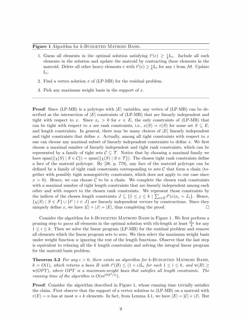
Figure 1 Algorithm for k-Budgeted Matroid Basis.

1. Guess all elements in the optimal solution satisfying `i(e) ≥ εkLi. Include all such

elements in the solution and update the matroid by contracting these elements in thematroid. Delete all other heavy elements e with `i(e) ≥ ε

kLi for any i fromM. UpdateLi.

2. Find a vertex solution x of (LP-MB) for the residual problem.

3. Pick any maximum weight basis in the support of x.

Proof: Since (LP-MB) is a polytope with |E| variables, any vertex of (LP-MB) can be de-scribed as the intersection of |E| constraints of (LP-MB) that are linearly independent andtight with respect to x. Since xe > 0 for e ∈ E, the only constraints of (LP-MB) thatcan be tight with respect to x are rank constraints, i.e., x(S) = r(S) for some set S ⊆ E,and length constraints. In general, there may be many choices of |E| linearly independentand tight constraints that define x. Actually, among all tight constraints with respect to xone can choose any maximal subset of linearly independent constraints to define x. We firstchoose a maximal number of linearly independent and tight rank constraints, which can berepresented by a family of tight sets C ⊆ T . Notice that by choosing a maximal family wehave span({χ(S) | S ∈ C}) = span({χ(S) | S ∈ T }). The chosen tight rank constraints definea face of the matroid polytope. By [38, p. 778], any face of the matroid polytope can bedefined by a family of tight rank constraints corresponding to sets C that form a chain (to-gether with possibly tight nonnegativity constraints, which does not apply to our case sincex > 0). Hence, we can choose C to be a chain. We complete the chosen rank constraintswith a maximal number of tight length constraints that are linearly independent among eachother and with respect to the chosen rank constraints. We represent those constraints bythe indices of the chosen length constraints J ⊆ {1 ≤ j ≤ k |

∑e∈E `

i(e)xe = Li}. Hence,{χ(S) | S ∈ F} ∪ {`i | i ∈ J} are linearly independent vectors by constructions. Since theyuniquely define x, we have |C|+ |J | = |E|, thus completing the proof. �

Consider the algorithm for k-Budgeted Matroid Basis in Figure 1. We first perform apruning step to guess all elements in the optimal solution with ith-length at least εLi

k for any1 ≤ i ≤ k. Then we solve the linear program (LP-MB) for the residual problem and removeall elements which the linear program sets to zero. We then select the maximum weight basisunder weight function w ignoring the rest of the length functions. Observe that the last stepis equivalent to relaxing all the k length constraints and solving the integral linear programfor the matroid basis problem.

Theorem 3.2 For any ε > 0, there exists an algorithm for k-Budgeted Matroid Basis,k = O(1), which returns a basis B with `i(B) ≤ (1 + ε)Li for each 1 ≤ i ≤ k, and w(B) ≥w(OPT ), where OPT is a maximum-weight basis that satisfies all length constraints. Therunning time of the algorithm is O(mO(k2/ε)).

Proof: Consider the algorithm described in Figure 1, whose running time trivially satisfiesthe claim. First observe that the support of a vertex solution to (LP-MB) on a matroid withr(E) = n has at most n+ k elements. In fact, from Lemma 3.1, we have |E| = |C|+ |J |. But

9

|C| ≤ r(E) since C is a chain and x(C) equals a distinct integer between 1 and r(E) for eachC ∈ C. Also |J | ≤ k proving the claim.

Let L′i be the ith budget of the residual problem solved in step 2 of the algorithm. Observethat the weight of the basis returned is at least the weight of the LP-solution and hence is atleast w(OPT ). Now, we show that the ith-length is at most L′i + εLi. Observe that any basismust contain r(E) elements out of the r(E) + k elements in the support. Hence, the longestith-length basis differs from the minimum ith-length basis by at most k · εkL′i = εL′i. But theminimum ith-length basis has ith-length at most the length of the fractional basis which isat most L′i. The claim follows. �

3.2 k-Budgeted Bipartite Matching

In this section we present a multi-criteria PTAS for k-Budgeted Bipartite Matching.We formulate the following linear programming relaxation (LP-BM) for the problem. We

use δ(v) to denote the set of edges incident to v ∈ V .

(LP-BM) maximize∑e∈E

w(e)xe

subject to∑e∈δ(v)

xe ≤ 1, ∀ v ∈ V

∑e∈E

`i(e)xe ≤ Li, ∀ 1 ≤ i ≤ k

xe ≥ 0, ∀ e ∈ E.

Consider the algorithm for k-Budgeted Bipartite Matching in Figure 2. Our algo-rithm works in three phases.

In the Preprocessing Phase, the algorithm guesses all the edges in OPT of weight at leastδw(OPT ) or ith-length at least δLi for some i. Here δ is a proper function of ε and k. Thisguessing can be performed in time polynomial in n (but exponential in δ). The algorithmthen includes all the guessed edges in the solution, and deletes the remaining heavy edgesand all edges incident to vertices which have already been matched by guessed edges. It alsoreduces the Li’s accordingly. After this phase w(e) ≤ δw(OPT ) and `i(e) ≤ δLi for each edgee.

In the Decomposition Phase our algorithm computes over a series of pruning and iterativesteps, a solution to the k-budgeted matching problem on a reduced graph that is eventuallya collection of paths. In Step (c), we discard nodes of degree 0 or of degree 3 or higher so asto leave only paths and cycles; Finally, one edge from each cycle is removed in this step. InStep (e), we further break each path into subpaths of bounded total weight and length. Thispruning is useful in the later Combination Phase when we choose one of the two matchingsin each path: the bounded difference ensures that one such combination is near optimal. Theuse of vertex solutions in all the residual problems ensures that the total number of edgesthrown away in all the above stages is roughly of the order of the extra budget constraintsin the problem which is O(k/γ) for a parameter γ ' O(ε/

√k). Finally, we output a feasible

fractional vertex solution xg to the LP with the following properties:

(1) The support of xg is a collection of vertex disjoint paths S1, . . . , Sh where h ≤ k.

10

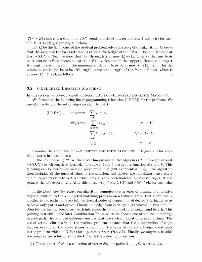
Figure 2 Algorithm for k-Budgeted Bipartite Matching.

Preprocessing

(a) Let δ = ε2 /(36k√

2k ln(k + 2)). Guess all the edges e in OPT such that w(e) ≥

δw(OPT ) or `i(e) ≥ δ Li for some i, and add them to the solution. Reduce the problemconsequently.

Decomposition

(b) Compute the optimal fractional vertex solution xb to LP-BM for the reduced problem.As long as there is an integral variable, reduce the problem appropriately and iterate.

(c) Remove all the nodes of degree zero and of degree at least 3, and all the edges incidentto the removed nodes. Compute an optimal fractional vertex solution xc to the problemLP-BM in the remaining graph. As long as there is an integral variable, reduce theproblem appropriately and iterate. Finally, remove one edge from each remaining cycle.

(d) Compute an optimal fractional vertex solution xd to the problem LP-BM in the remain-ing graph. As long as there is an integral variable, reduce the problem appropriatelyand iterate.

(e) Let γ = ε /(2√

2k ln(k + 2)). As long as there is a path P = (e1, e2, . . . , et) in the

support of xd such that w(P ) > γ w(xd) or `i(P ) > γ `i(xd) for some i, find a minimalprefix P ′ = (e1, e2, . . . , et′) of P satisfying the condition above and remove et′ from thegraph.

(f) Compute an optimal fractional vertex solution xf to the problem LP-BM in the remain-ing graph. As long as there is an integral variable, reduce the problem appropriatelyand iterate.

(g) Let P1, P2, . . . , Pq be the set of paths induced by xf . Return the subpaths S1, S2, . . . , Shformed after deleting the internal nodes whose matching constraints are not tight withrespect to xf . Return the solution xg which is xf induced on the edges in Si for each1 ≤ i ≤ h.

Combination

(h) LetMj and Mj be the two matchings partitioning Sj . Return the matchingM ′ satisfyingthe following properties: (i) For each Sj , M

′ ∩ Sj ∈ {Mj , Mj}; (ii) w(M ′) ≥ (1 −ε/2)w(xg) and `i(M ′) ≤ (1 + ε/2)`i(xg) for all i.

(2) xg is a (1 + ε/4)-approximate solution.

(3) For each Si, the degree constraints of the vertices of Si are tight except for its endpoints.

(4) For each Si, w · xg(Si) ≤ γ w(OPT ) and `i · xg(Sj) ≤ γLi for each 1 ≤ i ≤ k and1 ≤ j ≤ h where γ = ε/

(2√

2k ln(k + 2)).

In the final Combination Phase, the paths S1, . . . , Sh are used to compute an approximatefeasible (integral) solution. The algorithm enumerates over all the 2h matchings which areobtained by taking, for each Si, one of the two matchings which partition Si. This enumeration

11

takes polynomial time since h ≤ k = O(1). A probabilistic argument is used to show thatone of these matchings satisfies the claimed approximation guarantee of the algorithm.

Analysis. We now analyze the three phases of the algorithm, bounding the correspondingapproximation guarantee and running time. Consider first the Preprocessing Phase. In orderto implement Step (a), we have to consider all the possible choices, and run the algorithm foreach choice. Observe that there are at most (k+1)/δ such heavy edges in the optimal solution,and hence the number of possibilities is O(m(k+1)/δ) = O(mO(k2

√k log k/ε2)). The algorithm

generates a different subproblem for each possible guess of the edges. In the following we willfocus on the run of the algorithm where the guessed edges correspond to an optimal solution.

Consider now the Decomposition Phase. We prove that the output of this phase satisfiesthe four properties stated above. Observe that by construction the algorithm returns a col-lection of edge disjoint paths whose interior vertices have tight degree constraints. Properties(3) and (4) follow by construction. We now argue that the number of paths is bounded by k,proving Property (1).

Lemma 3.3 The number h of subpaths in Step (g) is upper bounded by k.

Proof: Consider the solution xf . The number of variables |E| =∑q

i=1 |Pi| is upper boundedby the number of tight constraints. Let q′ be the number of internal nodes whose matchingconstraint is not tight in xf . Note that the matching constraints at the endpoints of eachpath are not tight. Hence the number of tight constraints is at most

∑qi=1(|Pi|−1)− q′+k =

|E| − q − q′ + k ≥ |E|, from which q + q′ ≤ k. Observe that, by definition, the number hof subpaths is exactly q + q′ (we start with q subpaths, and create a new subpath for eachinternal node whose matching constraint is not tight). The claim follows. �

Clearly, solution xg satisfies all the constraints. We next argue that the weight of xg isnearly optimal. In Steps (c), (e) and (g) we remove a subset of edges whose optimal fractionalvalue is larger than zero in the step considered. In the following lemma we bound the numberof edges removed. Due to the Preprocessing Phase, the weight of these edges is negligible,which implies that the consequent worsening of the approximation factor is sufficiently small.This proves Property (2).

Lemma 3.4 The algorithm removes at most

1. 7k edges in Step (c);

2. (k + 1)/γ edges in Step (e);

3. 2k edges in Step (g).

Proof:(1) In the beginning of Step (c), all variables are strictly fractional. Thus, every vertex in V1,the set of vertices with tight degree constraints, has degree at least two. Let E be the residualedges. Note that |E| ≤ |V1|+ k since the number of tight constraints is at most |V1|+ k. LetH be the set of nodes of degree at least 3. Observe that

2(|V1|+ k) ≥ 2|E| ≥∑v∈V1

deg(v) ≥∑

v∈V1\H

2 +∑v∈H

deg(v) =⇒∑v∈H

deg(v) ≤ 2|H|+ 2k.

12

Since deg(v) ≥ 3 for each v ∈ H we have |H| ≤ 2k. Thus∑

v∈H deg(v) ≤ 6k.After removing nodes of degree 0 and at least 3, the graph consists of a set of paths

and cycles. Let C1, C2, . . . , Cq be the set of cycles, and P1, P2, . . . , Pr be the set of paths.We next show that q ≤ k with an analogous counting argument, and hence at most k moreedges are removed. Since G is bipartite, each cycle Ci must be even and therefore thecorresponding matching constraints must be dependent. Moreover, the endpoints of each pathcannot correspond to tight matching constraints. Thus the total number of edges over all sucheven cycles is |E| =

∑qi=1 |Ci|+

∑rj=1 |Pj | while the number of tight and independent degree

constraints and budget constraints is at most∑q

i=1(|Ci|−1)+∑r

j=1(|Pj |−1)+k = |E|−q−r+k.Since the number of variables is at most the number of tight and independent constraints atany vertex solution, we obtain that the number of cycles and paths altogether is at most k.(2) Each minimal subpath P ′ considered in Step (e) satisfies either w(P ′) > γ w(xd) or`i(P ′) > γ `i(xd) for some i. Since the edges of P ′ are not considered any more in thefollowing iterations of Step (e), the condition w(P ′) > γ w(xd) can be satisfied at most 1/γtimes. Similarly for the condition `i(P ′) > γ `i(xd). It follows that the number of minimalsubpaths, and hence the number of edges remove, is upper bounded by (k + 1)/γ.(3) Let V ′ be the set of internal vertices for which the degree constraints are not tight in thepaths P1, . . . , Pq and let V1 be the set of vertices with tight degree constraints. Thus, we havedeg(v) ≥ 2 for each v ∈ V1 ∪ V ′. But the total number of edges is at most |V1| + k. Thuswe have |V ′| ≤ k. We remove exactly two edges for each vertex in V ′ obtaining the claimedbound. �

Each of the steps (b) to (g) is run polynomially many times and takes polynomial time.Hence the overall running time of the Decomposition Phase is polynomial.

Consider eventually the Combination Phase. As described earlier, the running time of thisphase is bounded by O(2knO(1)). The following lemma, which is the heart of our analysis,shows that a subset M ′ satisfying Properties (i) and (ii) defined in the Combination Phase(h) always exists. Henceforth the algorithm always returns a solution. Although we usea randomized argument to prove the lemma, the algorithm is completely deterministic andenumerates over all solutions. Recall that Mj and Mj are the two matchings which partitionsubpath Sj .

Lemma 3.5 In Step (h) there is always a set of edges M ′ satisfying Properties (i) and (ii).

Proof: Consider the following packing problem

(PACK) maximize

h∑j=1

(yj w(Mj) + (1− yj) w(Mj))

subject to

h∑j=1

(yj `i(Mj) + (1− yj) `i(Mj)) ≤ Li, ∀ 1 ≤ i ≤ k

yj ∈ {0, 1}, ∀ 1 ≤ j ≤ h.

We can interpret the variables yj in the following way: M ′ ∩ Sj = Mj if yj = 1, andM ′ ∩Sj = Mj otherwise. Given a (possibly fractional and infeasible) solution y to PACK, we

use w(y) and `i(y) as shortcuts for∑h

j=1(yj w(Mj) + (1− yj) w(Mj)) and∑h

j=1(yj `i(Mj) +

(1− yj) `i(Mj)), respectively.

13

We first show that the solution xg can be interpreted as a feasible solution yg to the linearrelaxation of PACK as follows. Consider each subpath Sj . By definition, each matchingconstraint at an internal node of Sj is tight. This implies that all the edges e of Mj (resp.,Mj) have the same value xge =: yg (resp., xge =: 1− yg). Thus, we have w(yg) = w(xg).

Now, we construct an integral solution y′ in the following manner. Independently, foreach path Si, select Mi with probability ygi and Mi with probability 1 − ygi . Note thatE[w(y′)] = w(yg) and E[`i(y′)] = `i(yg) ≤ Li for all i. In order to prove the claim, it issufficient to show that, with positive probability, one has

w(y′) ≥ (1− ε/2)w(xg) and li(y′) ≤ (1 + ε/2)li(xg) for all i.

This implies that a matching satisfying (i) and (ii) always exists, and hence the algorithmwill find it.

By Step (e), switching one variable of y′ from 1 to 0 or vice versa can change the cost andith-length of y′ at most by γ w(xg) and γ `i(xg), respectively. Using the method of boundeddifferences (see, e.g., [29]):

Pr(w(y′) < E[w(y′)]− t) ≤ e−t2

2h(γ w(xg))2 and Pr(`i(y′) > E[`i(y′)] + t) ≤ e−t2

2h(γ `i(xg))2 .

Recalling that E[w(y′)] ≥ w(xg), h ≤ k, and setting t = ε/2 · w(xg) = γ w(xg)√

2k ln(k + 2),

Pr(w(y′) < w(xg)− ε/2 · w(xg)) ≤ Pr(w(y′) < E[w(y′)]− γ w(xg)√

2k ln(k + 2))

≤ e−(γ w(xg))2 2k ln(k+2)/2h(γw(xg))2 ≤ e− ln(k+2) =1

k + 2.

Similarly, for all i,

Pr(`i(y′) > `i(xg) + ε/2 · `i(xg)) ≤ 1

k + 2.

From the union bound, the probability that y′ does not satisfy Property (ii) is therefore atmost k+1

k+2 < 1. The claim follows. �

Theorem 3.6 . For any ε > 0, there exists a deterministic algorithm for k-BudgetedBipartite Matching, k = O(1), which returns a matching M of weight w(M) ≥ (1 −ε)w(OPT ) and length `i(M) ≤ (1 + ε)Li for each 1 ≤ i ≤ k. The running time of thealgorithm is O(nO(k2

√k log k/ε2)).

Proof: Consider the above algorithm, whose running time is trivially as in the claim. It iseasy to see that the solution returned is a matching. Moreover a solution is always returnedby Lemma 3.5. The approximation guarantee of the algorithm follows from the properties ofthe Decomposition step and Lemma 3.5. �

4 Pure Approximation Schemes for Independence Systems

In this section we present our pure approximation schemes (which do not violate any budgetconstraint) when the solution space F is an independence system, i.e. if F ∈ F and F ′ ⊆ F

14

then F ′ ∈ F . We start by describing our feasibilization mechanism to turn multi-criteriaapproximation schemes into pure approximation schemes. We then present our deterministicapproximation scheme for matroid independent set. We conclude the section with a deter-ministic approximation scheme for matchings (in general graphs) with k budget constraints,where k = (1) as usual.

4.1 A Feasibilization Mechanism

Since we deal with independence systems, minimization problems are trivial (the empty so-lution is optimal). Therefore, we will consider maximization problems only. Analogous toterminology used in matroid theory, for an independence system F on some ground set Eand any I ∈ F , we call the independence system {S ∈ E \ I | S ∪ I ∈ F} on ground set E \ Ia contraction of F . Similarly, for any I ⊆ E, the independence system {S ∈ E \ I | S ∈ F}is called a restriction of F . Combination of contractions and restrictions are called minors.We say that a family F of independence systems is self-reducible if it is closed under takingminors. Self-reducibility is a natural property for independence system, examples includefeasible solutions to knapsack problems, graphic matroids, linear matroids, matchings, andbipartite matchings.

Theorem 4.1 (Feasibilization) Let F be a self-reducible family of independence systems.Suppose that we are given an algorithm A which, for any constant δ > 0 and k-budgetedoptimization problem Pind on an independence system F ∈ F , computes in polynomial timea solution S ∈ F to the k-budgeted maximization problem on F of cost (resp., expected cost)at least (1− δ) times the optimum in F , violating each budget by a factor of at most (1 + δ).Then there is a PTAS (resp., PRAS) for Pind.5

Proof: Let ε ∈ (0, 1] be a given constant, with 1/ε ∈ N. Consider the following algorithm.Initially we guess the h = k/ε elements EH of OPT of largest weight, and reduce the problemconsequently, hence getting a problem P ′. Then we scale down all the budgets by a factor(1− δ), and solve the resulting problem P ′′ by means of A, where δ = ε/(k + 1). Let EL bethe solution returned by A. We finally output EH ∪ EL.

Let OPT ′ and OPT ′′ be the optimum solution to problems P ′ and P ′′, respectively. Wealso denote by L′i and L′′i the ith budget in the two problems, respectively. Let wmax be thelargest weight in P ′ and P ′′. We observe that trivially: (a) w(OPT ) = w(EH) + w(OPT ′)and (b) wmax ≤ w(EH)/h.

Let us show that (c) w(OPT ′′) ≥ w(OPT ′)(1 − kδ) − kwmax. Consider the followingprocess: for each length function i, we remove from OPT ′ the element e with smallest ratiow(e)/`i(e) until the remaining elements of OPT’ have ith length ≤ (1− δ)L′i. Let Ei be theset of elements removed. More formally, we number the elements of OPT ′ = {e1, e2, . . . , eq}such that w(e1)/`i(e1) ≤ w(e2)/`i(e2) ≤ · · · ≤ w(eq)/`

i(eq). Hence, Ei = {e1, . . . , er}, wherer ∈ {0, . . . , q} is the smallest index such that `i({er+1, . . . , eq}) ≤ (1 − δ)L′i. We now showw(Ei) ≤ δw(OPT ′) + wmax. This is trivially true if Ei = ∅, hence, we assume without loss ofgenerality r ≥ 1. Since `i(OPT ′) ≤ L′i and r is the smallest index with `i({er+1, . . . , eq}) ≤(1− δ)L′i, or equivalently `i({e1, . . . , er}) ≥ `i(OPT ′)− (1− δ)L′i, we get

`i({e1, . . . , er−1}) < `i(OPT ′)− (1− δ)L′i ≤ δ`i(OPT ′). (1)

5Notice that it suffices to assume that F is closed under contractions, since a restriction can be emulatedby setting the weights of the elements to be removed to zero.

15

Furthermore, notice that for any four reals A,B, a, b > 0 with AB ≥

ab , we have a+A

b+B ≥ab .

Applying this inequality repeatedly, we obtain

w(e1)

`i(e1)≤ w({e1, e2})`i({e1, e2})

≤ · · · ≤ w(OPT ′)

`i(OPT ′),

and in particularw({e1, . . . , er−1})`i({e1, . . . , er−1})

≤ w(OPT ′)

`i(OPT ′). (2)

Hence,

w(Ei) = w(er) + w({e1, . . . , er−1})(2)

≤ wmax + `i({e1, . . . , er−1}) ·w(OPT ′)

`i(OPT ′)

(1)

≤ wmax + δw(OPT ′),

as claimed. It follows that OPT ′ − ∪iEi is a feasible solution for P ′′ of weight at leastw(OPT ′)(1− δk)− kwmax, proving (c).

We observe that EL is feasible for P ′ since, for each i, `i(EL) ≤ (1 + δ)L′′i = (1 + δ)(1 −δ)L′i ≤ L′i. As a consequence, the returned solution EH ∪EL is feasible. Moreover, when A isdeterministic, we have

w(EH) + w(EL) ≥ w(EH) + (1− δ)w(OPT ′′)

(c)

≥ w(EH) + (1− δ)(w(OPT ′)(1− δk)− kwmax)

(b)

≥ (1− k/h)w(EH) + (1− δ(k + 1))w(OPT ′)

≥ (1− ε)(w(EH) + w(OPT ′))(a)= (1− ε)w(OPT ).

The same bound holds in expectation when A is randomized. �

Corollary 4.2 There are PTASs for k-budgeted forest and k-budgeted bipartitematching. There are PRASs for k-budgeted matching, k-budgeted matroid inde-pendent set, and k-budgeted matroid intersection in representable matroids.

Proof: The result about bipartite matching follows from the multi-criteria PTAS in pre-vious section. All the other results follow from known multi-criteria PTASs and PRASs[5, 9, 10, 30, 32]. �

4.2 A PTAS for k-Budgeted Matroid Independent Set

Again, we denote by r(S) = max{|J | | J ⊆ S, J ∈ I} the rank function of a matroidM = (E, I). Furthermore, PI = {x ≥ 0 | x(S) ≤ r(S) ∀S ⊆ E} denotes the matroid polytopewhich is the convex hull of the characteristic vectors χI of the independent sets I ∈ I.

16

Theorem 4.3 Let M = (E, I) be a matroid and let F be a face of dimension d of the matroidpolytope PI . Then any x ∈ F has at most 2d non-integral components. Furthermore, the sumof all fractional components of x is at most d.

Proof: Letm = |E|. We assume that the matroid polytope has full dimension, i.e., dim(PI) =m, or equivalently, every element e ∈ E is independent. This can be assumed w.l.o.g. sinceif {e} 6∈ I for some e ∈ E, then we can reduce the matroid by deleting element e. By [38,p. 778], any d-dimensional face F of a polymatroid, which is a generalization of a matroidpolytope, can be described as follows

F = {x ∈ PI | x(e) = 0 ∀e ∈ N, x(Ai) = r(Ai) ∀i ∈ {1, . . . , k}},

where A1 ( A2 ( · · · ( Ak ⊆ E, and N ⊆ E with |N | + k = m − d. We prove the claim byinduction on the number of elements of the matroid. The theorem clearly holds for matroidswith a ground set of cardinality one. First assume N 6= ∅ and let e ∈ N . Let M ′ be thematroid obtained from M by deleting e, and let F ′ be the projection of F onto the coordinatescorresponding to N \{e}. Since F ′ is a face of M ′, the claim follows by induction. Henceforth,we assume N = ∅ which implies k = m− d. Let A0 = ∅ and Bi = Ai \Ai−1 for i ∈ {1, . . . , k}.In the following we show that we can assume

0 < r(Ai)− r(Ai−1) < |Bi| ∀ i ∈ {1, . . . , k}. (3)

Notice that 0 ≤ r(Ai)− r(Ai−1) ≤ |Bi| clearly holds by standard properties of rank functions(see [38, p. 664] for more details). Assume that there is i ∈ {1, . . . , k} with r(Ai) = r(Ai−1).Since all points x ∈ F satisfy x(Ai) = r(Ai) and x(Ai−1) = r(Ai−1), we have x(Bi) = 0.Hence for any e ∈ Bi, we have x(e) = 0 for x ∈ F . Again, we can delete e from the matroid,hence obtaining a smaller matroid for which the claim holds by the inductive hypothesis.Therefore, we can assume r(Ai) > r(Ai−1) which implies the left inequality in (3).

For the right inequality assume that there is i ∈ {1, . . . , k} with r(Ai) − r(Ai−1) = |Bi|.Hence, every x ∈ F satisfies x(Bi) = |Bi|, implying x(e) = 1 for all e ∈ Bi. Let e ∈ Bi, andlet F ′ be the projection of the face F onto the components N \ {e}. Since F ′ is a face ofthe matroid M ′ obtained from M by contracting e, the result follows again by the inductivehypothesis.

Henceforth, we assume that (3) holds. This implies in particular that |Bi| > 1 for i ∈{1, . . . , k}. Since

∑ki=1 |Bi| ≤ m, we have k ≤ m/2, which together with k = m − d implies

d ≥ m/2. The claim of the theorem that x ∈ F has at most 2d non-integral components isthus trivial in this case.

To prove the second part of the theorem we show that if (3) holds then x(E) ≤ d forx ∈ F . For x ∈ F we have

x(E) = x(E \Ak) +

k∑i=1

x(Bi)

≤ |E| − |Ak|+k∑i=1

(r(Ai)− r(Ai−1))

≤ |E| − |Ak|+k∑i=1

(|Ai| − |Ai−1| − 1)

= m− k = d,

17

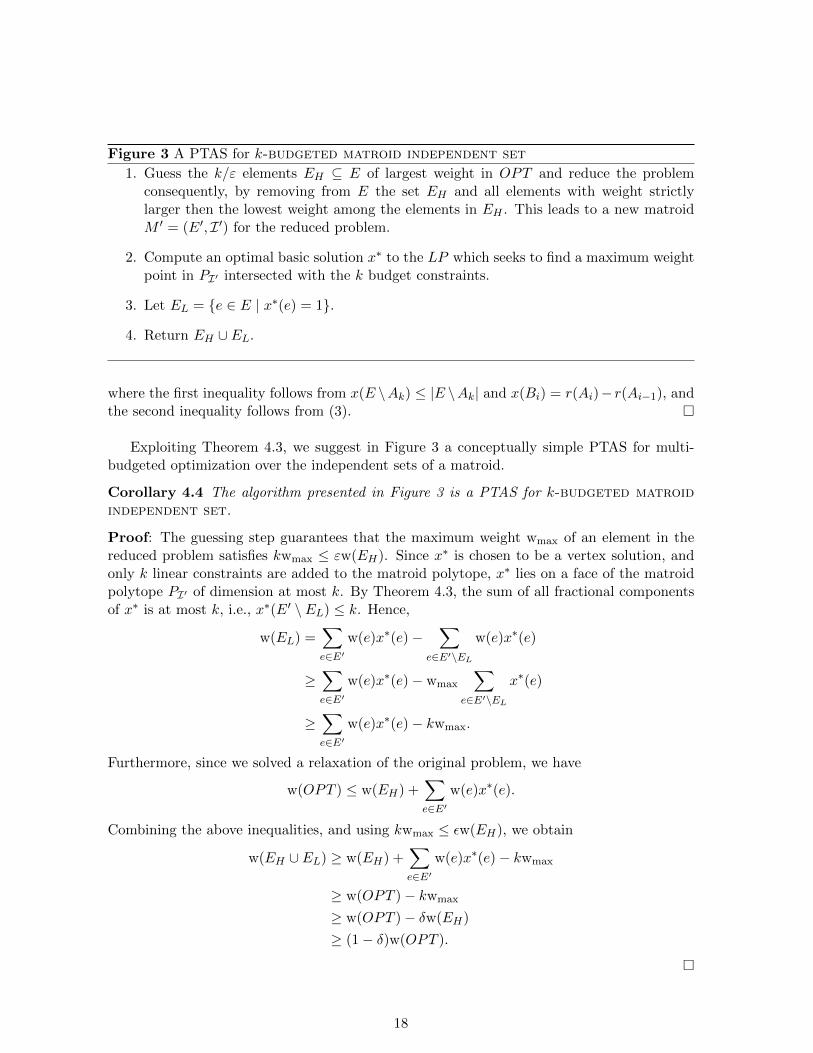
Figure 3 A PTAS for k-budgeted matroid independent set

1. Guess the k/ε elements EH ⊆ E of largest weight in OPT and reduce the problemconsequently, by removing from E the set EH and all elements with weight strictlylarger then the lowest weight among the elements in EH . This leads to a new matroidM ′ = (E′, I ′) for the reduced problem.

2. Compute an optimal basic solution x∗ to the LP which seeks to find a maximum weightpoint in PI′ intersected with the k budget constraints.

3. Let EL = {e ∈ E | x∗(e) = 1}.

4. Return EH ∪ EL.

where the first inequality follows from x(E \Ak) ≤ |E \Ak| and x(Bi) = r(Ai)− r(Ai−1), andthe second inequality follows from (3). �

Exploiting Theorem 4.3, we suggest in Figure 3 a conceptually simple PTAS for multi-budgeted optimization over the independent sets of a matroid.

Corollary 4.4 The algorithm presented in Figure 3 is a PTAS for k-budgeted matroidindependent set.

Proof: The guessing step guarantees that the maximum weight wmax of an element in thereduced problem satisfies kwmax ≤ εw(EH). Since x∗ is chosen to be a vertex solution, andonly k linear constraints are added to the matroid polytope, x∗ lies on a face of the matroidpolytope PI′ of dimension at most k. By Theorem 4.3, the sum of all fractional componentsof x∗ is at most k, i.e., x∗(E′ \ EL) ≤ k. Hence,

w(EL) =∑e∈E′

w(e)x∗(e)−∑

e∈E′\EL

w(e)x∗(e)

≥∑e∈E′

w(e)x∗(e)− wmax

∑e∈E′\EL

x∗(e)

≥∑e∈E′

w(e)x∗(e)− kwmax.

Furthermore, since we solved a relaxation of the original problem, we have

w(OPT ) ≤ w(EH) +∑e∈E′

w(e)x∗(e).

Combining the above inequalities, and using kwmax ≤ εw(EH), we obtain

w(EH ∪ EL) ≥ w(EH) +∑e∈E′

w(e)x∗(e)− kwmax

≥ w(OPT )− kwmax

≥ w(OPT )− δw(EH)

≥ (1− δ)w(OPT ).

�

18

4.3 A PTAS for k-BUDGETED MATCHING

In this section we present our PTAS for k-budgeted matching. We denote byM the set ofincidence vectors of matchings. With a slight abuse of terminology we call the elements inMmatchings. Let PM be the matching polytope. To simplify the exposition, it is convenient toconsider weights w and lengths `i for i ∈ {0, . . . , k} sometimes as vectors in QE

+. We denoteby ` = (`1, . . . , `k) the matrix whose ith column is `i, and let L = (L1, . . . ,Lk)

T be the vectorcorresponding to the budgets. Using this terminology, a feasible solution to the k-budgetedmatching problem is a matching x ∈M such that `Tx ≤ L.

We will first describe a procedure that returns a feasible matching of weight at least

w(OPT ) − (k+3)k2

k+1 wmax, where wmax = max{w(e) | e ∈ E}. Similar to the algorithms seen

in previous sections, it then suffices to perform a preprocessing step to guess the d (k+3)k2

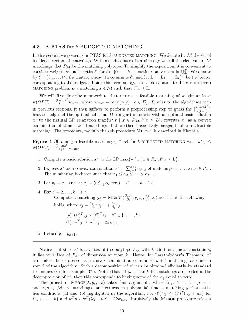
ε(k+1) eheaviest edges of the optimal solution. Our algorithm starts with an optimal basic solutionx∗ to the natural LP relaxation max{wTx | x ∈ PM, `Tx ≤ L}, rewrites x∗ as a convexcombination of at most k+1 matchings that are then successively merged to obtain a feasiblematching. The procedure, modulo the sub procedure Merge, is described in Figure 4.

Figure 4 Obtaining a feasible matching y ∈ M for k-budgeted matching with wT y ≤w(OPT )− (k+3)k2

k+1 wmax.

1. Compute a basic solution x∗ to the LP max{wTx | x ∈ PM, `Tx ≤ L}.

2. Express x∗ as a convex combination x∗ =∑k+1

j=1 αjxj of matchings x1, . . . , xk+1 ∈ PM.The numbering is chosen such that α1 ≤ α2 ≤ · · · ≤ αk+1.

3. Let y1 = x1, and let βj =∑j

r=1 αr for j ∈ {1, . . . , k + 1}.

4. For j = 2, . . . , k + 1 :Compute a matching yj = Merge(

βj−1

βj, yj−1,

αjβj, xj) such that the following

holds, where zj =βj−1

βjyj−1 +

αjβjxj :

(a) (`i)T yj ≤ (`i)T zj ∀i ∈ {1, . . . , k},(b) wT yj ≥ wT zj − 2kwmax.

5. Return y = yk+1.

Notice that since x∗ is a vertex of the polytope PM with k additional linear constraints,it lies on a face of PM of dimension at most k. Hence, by Caratheodory’s Theorem, x∗

can indeed be expressed as a convex combination of at most k + 1 matchings as done instep 2 of the algorithm. Such a decomposition of x∗ can be obtained efficiently by standardtechniques (see for example [37]). Notice that if fewer than k+ 1 matchings are needed in thedecomposition of x∗, then this corresponds to having some of the αj equal to zero.

The procedure Merge(λ, y, µ, x) takes four arguments, where λ, µ ≥ 0, λ + µ = 1and x, y ∈ M are matchings, and returns in polynomial time a matching y that satis-fies conditions (a) and (b) highlighted in the algorithm, i.e, (`i)T y ≤ (`i)T (λy + µx) fori ∈ {1, . . . , k} and wT y ≥ wT (λy + µx)− 2kwmax. Intuitively, the Merge procedure takes a

19

point z = λy + (1 − λ)x on an edge of the matching polytope PM and returns a matchingy with weight and lengths similar to z. We give the details of Merge later, and first showthe following, assuming that Merge returns a matching with the properties described in thealgorithm.

Theorem 4.5 Given an efficient Merge procedure fulfilling the requirements described inthe algorithm in Figure 4, the algorithm in Figure 4 is an efficient procedure that returns a

feasible matching y for k-budgeted matching with wT y ≤ w(OPT )− (k+3)k2

k+1 wmax.

Proof: The algorithm is clearly efficient.To prove feasibility of y = yk+1, we fix i ∈ {1, . . . , k} and show by induction on j ∈

{1, . . . , k + 1} that

(`i)T yj ≤ (`i)T

(1

βj

j∑r=1

αrxr

). (4)

Feasibility then follows from feasibility of x∗ since

(`i)T yk+1

(4)

≤ (`i)T

(1

βk+1

k+1∑r=1

αrxr

)= (`i)Tx∗ ≤ Li.

Since y1 = x1, (4) trivially holds for j = 1. Furthermore, let j ∈ {1, . . . , k} and assumethat (4) holds for any value less or equal to j. Then using property (a) of Merge, we obtain

(`i)T yj+1

(a)

≤ (`i)T zj+1 = (`i)T(

βjβj+1

yj +αj+1

βj+1xj+1

)ind. hyp. (4)

≤ (`i)T

(1

βj+1

j+1∑r=1

αrxr

),

thus proving (4) and implying feasibility of y.Similarly, to prove that y has large weight, we show by induction on j ∈ {1, . . . , k + 1}

that

wT yj ≥1

βj

(wT

(j∑r=1

αrxr

)−

(j∑r=2

βr

)2kwmax

). (5)

The desired result on the weight of y = yk+1 then follows by observing that βr ≤ rk+1 , since

α1 ≤ · · · ≤ αk+1, and

wT yk+1

(5)

≥ wT

(k+1∑r=1

αrxr

)−

(k+1∑r=2

βr

)2kwmax

≥ wTx∗ −

(k+1∑r=2

r

k + 1

)2kwmax

= w(OPT )− (k + 3)k2

k + 1wmax.

Again, (5) is trivially true for j = 1 since y1 = x1. Furthermore, for j ∈ {1, . . . , k} we obtain

20

the following by using property (b) of Merge:

wT yj+1

(b)

≥ wT zj+1 − 2kwmax =1

βj+1wT (βjyj + αj+1xj+1)− 2kwmax

ind. hyp. (5)

≥ 1

βj+1

(wT

(j∑r=1

αrxr

)−

(j∑r=2

βr

)2kwmax + wT (αj+1xj+1)

)− 2kwmax

=1

βj+1

(wT

(j+1∑r=1

αrxr

)−

(j+1∑r=2

βr

)2kwmax

).

�

Hence, it remains to present an efficient Merge procedure fulfilling property (a) and (b).

4.3.1 Merging procedure

Consider fixed input parameters x′, x′′ ∈M and α ∈ [0, 1] of Merge(α, x′, 1−α, x′′). Mergeworks in two steps. First, it constructs a fractional point y ∈ [0, 1]E that is structurally closeto being a matching in a well-defined sense, and satisfies

wT y = wT (αx′ + (1− α)x′′), and (6)

(`i)T y = (`i)T (αx′ + (1− α)x′′) ∀i ∈ {1, . . . , k}. (7)

In a second step y is transformed to a matching with the desired properties.More precisely, we want y to be a 2k-almost matching, defined as follows.

Definition 4.6 (r-almost matching) For r ∈ N, a vector y ∈ [0, 1]E is an r-almost match-ing in G = (V,E) if it is possible to set at most r components of y to zero to obtain a matching.We denote by Mr the set of all r-almost matchings.

Given an r-almost matching y, we say that z is a corresponding matching (to y), if it isa matching obtained by setting at most r components of y to zero. Such a correspondingmatching z can easily be found by first setting all fractional components of y to zero, andthen computing a maximum cardinality matching in the resulting set of edges. Clearly, acorresponding matching z satisfies wT z ≥ wT y−rwmax. Hence, to obtain a Merge procedurewith the desired properties, it indeed suffices to present an efficient procedure to construct a2k-almost matching y that satisfies (6) and (7): a corresponding matching z clearly has lowerlengths, since z ≤ y, and

wT z ≥ wT y − 2kwmax = wT (αx′ + (1− α)x′′)− 2kwmax,

by the above observation and (7). Hence, we now focus on efficiently getting a 2k-almostmatching y satisfying (6) and (7).

To construct y, we start with x′ and define a way to fractionally swap parts of x′ withx′′. For this we define a generalized symmetric difference. For two vectors z′, z′′ ∈ [0, 1]E , wedefine their symmetric difference z′∆z′′ ∈ [0, 1]E by (z′∆z′′)(e) = |z′(e)− z′′(e)| for all e ∈ E.In particular, if z′ and z′′ are incidence vectors, then their symmetric difference as defined

21

above corresponds indeed to the symmetric difference in the usual sense. Recall that, whenz′ and z′′ are matchings, z′∆z′′ consists of a set of node-disjoint paths and cycles.

Consider the paths and cycles in s = x′∆x′′. We number the edges {e0, . . . , eτ−1} in ssuch that two consecutively numbered edges are either consecutive in some path/cycle or be-long to different paths/cycles. This can easily be achieved by cutting each cycle, appendingthe resulting set of paths one to the other, gluing together the endpoints of the obtainedpath, and then number consecutively the edges in the obtained path. For t ∈ [0, τ ], we defines(t) ∈ [0, 1]E as

(s(t))(e) =

1 if e = ei, i ∈ {0, . . . , btc};t− btc if e = ei, i = btc and i ≤ τ − 1;

0 otherwise.

Furthermore, for a, b ∈ [0, τ ] we define s(a, b) ∈ [0, 1]E as follows

s(a, b) =

{s(b)− s(a) if a ≤ b,s(a) + s(τ)− s(b) if a > b.

Hence, s(a, b) can be interpreted as a fractional version of a cyclic interval of edges in s. Wedenote by [a, b] , the cyclic interval contained in [0, τ ], which is defined by

[a, b] =

{[a, b] if a ≤ b,[0, a] ∪ [b, τ ] if a > b.

Notice that for a, b ∈ [0, τ ], the vector y = x′∆s(a, b) is a 2-almost matching since toobtain a matching, it suffices to set the coordinates of y that correspond to ebac and ebbc tozero. Analogously, for any family of k disjoint cyclic intervals [a1, b1] . . . [ak, bk] ⊆ [0, τ ],the vector

y = x′∆s(a1, b1)∆ . . .∆s(ak, bk) (8)

is a 2k-almost matching. We will find k disjoint cyclic intervals such that y as defined in (8)satisfies (6) and (7).

We first prove non-constructively the existence of intervals [a1, b1] , . . . , [ak, bk] that leadto a desired y, using the following slight generalization of a Theorem of Stromquist andWoodall [40]. In the theorem below, a signed measure denotes the difference between twofinite measures. Furthermore, we call a measure non-atomic if every singleton has measurezero.

Theorem 4.7 Let d ≥ 2, and let µ1, . . . , µd be non-atomic signed measures on [0, 1]. Foreach λ ∈ [0, 1] there is a set Kλ ⊆ [0, 1] that is the union of at most d − 1 circular intervalsof [0, 1] and satisfies µi(Kλ) = λµi([0, 1]) ∀i ∈ {1, . . . , d}.

The difference between Theorem 4.7 and [40, Theorem 1] is that we allow for signedmeasures instead of usual measure. Even though Theorem 4.7 is a direct generalization ofStromquist and Woodall’s Theorem, for completeness, we provide a proof in Section 4.3.2.Notice that Theorem 4.7 could be equivalently stated for the interval [0, τ ] instead of [0, 1].Based on Theorem 4.7 we obtain the following.

22

Theorem 4.8 There exist k disjoint cyclic intervals [a1, b1] , . . . , [ak, bk] ⊆ [0, τ ], some ofwhich may be empty, such that the vector

y = x′∆s(a1, b1)∆ . . .∆s(ak, bk)

satisfies (6) and (7).

Proof: We define the following k+1 signed measures µ1, . . . , µk+1 on [0, τ ] by providing theirvalues on subintervals of [0, τ ]. For [a, b) ⊆ [0, τ ], let

µi([a, b)) = (`i)T (x′∆s(a, b)− x′) ∀i ∈ {1, . . . , k},µk+1([a, b)) = wT (x′∆s(a, b)− x′).

In particular, for any cyclic interval [a, b] ⊆ [0, τ ], µi([a, b] ) and µk+1([a, b] ) measure thechange in the ith length and weight, respectively, when replacing x′ by x′∆s(a, b). Moregenerally, for k disjoint cyclic intervals [a1, b1] , . . . , [ak, bk] and the vector

y = x∆s(a1, b1)∆ . . .∆s(ak, bk), (9)

we have(`i)T y = (`i)Tx′ + µi(∪kj=1[aj , bj ] ) i ∈ {1, . . . , k},

wT y = wTx′ + µk+1(∪kj=1[aj , bj ] ).(10)

Furthermore, it is easy to check that µi for i ∈ {1, . . . , k + 1} are non-atomic signed mea-sures. Hence, using Theorem 4.7 with λ = 1 − α, there exist disjoint circular intervals[a1, b1] , . . . , [ak, bk] ⊆ [0, τ ] such that

µi(∪kj=1[aj , bj ] ) = (1− α)µi([0, τ ]) ∀i ∈ {1, . . . , k + 1}.

Consider y being defined as in (9) for those intervals. Then combining the above equalitywith (10) we obtain

(`i)T y = (`i)Tx′ + (1− α)µi([0, τ ])

= (`i)Tx′ + (1− α)(`i)T (x′′ − x′)= (`i)T (αx′ + (1− α)x′′), ∀i ∈ {1, . . . , k},

and similaly,

wT y = wTx′ + (1− α)w([0, τ ])

= wTx′ + (1− α)wT (x′′ − x′)= wT (αx′ + (1− α)x′′),

as desired. �

Theorem 4.9 A set of k cyclic intervals as described in Theorem 4.8 can be found efficiently.

23

Proof: Notice that we can efficiently guess bajc and bbjc for j ∈ {1, . . . , k} for a set of cyclicintervals [a1, b1] , . . . , [ak, bk] ⊆ [0, τ ] guaranteed to exist by Theorem 4.8. More precisely,there are only O(τ2k) possibilities. Since τ is bounded by the number of vertices and k is aconstant, this is polynomial. Futhermore, when the integer part of ai, bi for j ∈ {1, . . . , k} isfixed, then the vector

y = x′∆s(a1, b1)∆ . . .∆s(ak, bk)

is linear in the aj ’s and bj ’s. Therefore (`i)T y for i ∈ {1, . . . , k} and wT y are linear in the aj ’sand bj ’s. Hence, finding values of the aj ’s and bj ’s, with predetermined integer parts, suchthat the resulting y satisfies (6) and (7), reduces to solving a constant-size linear problem,which can be done in constant time. �

Summarizing the above discussion, we get the following.

Corollary 4.10 There is an efficient procedure Merge(α, x′, 1 − α, x′′), that for α ∈ [0, 1],and x′, x′′ ∈M, outputs a matching y satisfying (6) and (7).

This finishes the description of the algorithm in Figure 4 and implies together with The-orem 4.5 the following.

Corollary 4.11 The algorithm described in Figure 4 is an efficient procedure that returns a

feasible matching y for k-Budgeted Matching with wT y ≥ w(OPT )− (k+3)k2

k+1 wmax.

To obtain a PTAS for k-budgeted matching, it suffices to guess the d (k+3)k2

(k+1)ε e heaviestedges of an optimal solution before applying the algorithm in Figure 4.

Theorem 4.12 Let ε > 0. The following procedure is an efficient (1− ε)-approximation fork-budgeted matching.

1. Guess the d (k+3)k2

(k+1)ε e heaviest edges EH of an optimal solution, and reduce the problemcorrepondingly.

2. Apply the algorithm in Figure 4 to the reduced problem to get a matching EL.

3. Return EH ∪ EL.

Proof: Efficiency and feasibility is obvious. We have to show w(EH ∪EL) ≥ (1− ε)w(OPT ).Let w′max be the maximum weight of an edge in the reduced problem. Since, to build thereduced problem, we remove all edges of weight strictly larger then the smallest weight inEH , we have

w′max ≤ w(e) ∀e ∈ EH . (11)

Furthermore, let OPT ′ be an optimal solution in the reduced problem. Clearly

w(OPT ) = w(EH) + w(OPT ′). (12)

Hence,

w(EH ∪ EL) = w(EH) + w(EL)Cor. 4.11≥ w(EH) + w(OPT ′)− (k + 3)k2

k + 1w′max

(11)

≥ w(EH) + w(OPT ′)− εw(EH) ≥ (1− ε)(w(EH) + w(OPT ′))

(12)= (1− ε)w(OPT ).

24

�

For completeness, the following section shows how Theorem 4.7 is obtained by followingthe proof of Stromquist and Woodall [40, Theorem 1].

4.3.2 A generalization of a Theorem by Stromquist and Woodall

To prove Theorem 4.7 we use the same proof technique as [40] with the only difference that wereplace the classical version of the Ham Sandwich Theorem by the following generalization.

Theorem 4.13 (Generalized Ham Sandwich Theorem) Suppose we are given d signedmeasures µ1, . . . , µd on Rd that vanish on any hyperplane, then there exists a (possible degen-erate) halfspace H in Rd such that

µi(H) =1

2µi(Rd) ∀i ∈ {1, . . . , d},

where a degenerate halfspace is either ∅ or Rd.

Theorem 4.13 with the additional requirement of the µi being absolutely continuous wasproven in [2]. Their proof follows a standard approach used in [41] to show the classic HamSandwich Theorem for (unsigned) measures, which is based on the Borsuk-Ulam Theorem [3].However, the proof presented in [2] actually shows Theorem 4.13, and was only stated in aslightly weaker form requiring absolute continuity of the measures.

For completeness, we replicate the proof of Stromquist and Woodall, in a slightly gener-alized version that uses Theorem 4.13, to show Theorem 4.7.

Proof:[of Theorem 4.7, following [40]] We denote by A ⊆ [0, 1] the values of λ ∈ [0, 1] forwhich the statement is true. We have to show that A = [0, 1]. This will follow from thefollowing four statements:

(a) 1 ∈ A,

(b) λ ∈ A⇒ (1− λ) ∈ A,

(c) λ ∈ A⇒ 12λ ∈ A,

(d) A is closed.

Statement (a) follows by choosing K1 = [0, 1], and (b) by setting K1−λ = [0, 1] \ Kλ.Furthermore, (d) follows by observing that the space of the unions of d − 1 intervals iscompact in a suitable topology, hence, for any sequence of λ’s in A, the corresponding Kλ’sconverge. It remains to prove (c).

Fix λ ∈ A and let Kλ ⊆ [0, 1] be a union of d − 1 cyclic intervals of [0, 1] such thatµi(Kλ) = λµi(Rd) for i ∈ {1, . . . , d}. If Kλ 6= [0, 1], we can assume that the origin is notcontained in Kλ, for otherwise, we can simply reparameterize the circular interval [0, 1]. Letf : [0, 1)→ Rn be defined by

f(t) = (t, t2, . . . , td).

We will apply the generalized Ham Sandwich Theorem 4.13 to a family of measures withsupport included in the image of f . More precisely, we define d measures ν1, . . . , νd on Rd by

νi(B) = µi(f−1(B) ∩Kλ) ∀i ∈ {1, . . . , d}, B ⊆ Rd Borel set.

25

Notice that νi(Rd) = µi(Kλ) = λµi(Rd), and νi are signed measures. Furthermore, forany hyperplane X in Rd, f−1(X) is a set of size at most d, and since the measures µi arenon-atomic, this implies νi(X) = 0. Hence, we can apply the Generalized Ham SandwichTheorem 4.13 to obtain that there exists a halfspace H ⊂ Rd such that νi(H) = λ

2µi(Rd)

for i ∈ {1, . . . , d}. Let X be the hyperplane that is the boundary of H. Consider thecomplementary halfspace H of H, i.e, H ∩H = X. Since νi(Rd) = λµi(Rd) for i ∈ {1, . . . , d},we also have νi(H) = λ

2µi(Rd) for i ∈ {1, . . . , d}. We will show that one can choose Kλ

2to be

either KH := f−1(H) ∩Kλ or KH := f−1(H) ∩Kλ. Notice that νi(H) = νi(H) = λ2µi(R

d)for i ∈ {1, . . . , d} can be rephrased as

µi(KH) = µi(K

H) =λ

2µi(Rd) ∀i ∈ {1, . . . , d}.

Hence, both KH and KH have the desired mass with respect to the measures µ1, . . . , µd. Itremains to show that one of them is a union of at most d intervals.

Since |f−1(X) ∩Kλ| ≤ d, the ≤ d intervals of Kλ are hit in at most d points by f−1(X),thus subdividing Kλ into at most 2d+1 intervals. These intervals are partitioned by KH andKH . Hence, indeed, either KH or KH is the union of at most d intervals. �

Conclusions

We presented approximation algorithm for a variety of multi-budgeted problems. A maindrawback of the procedures presented here is the quite high dependence of the running timeon the (constant) number of budgets. It is an interesting question whether FPTASs can bedesigned for problems presented in this paper, as for example k-budgeted matching. Themain reason why the presented procedures do not lead to FPTASs is the use of guessingsteps. This includes the guessing of a number of element that depends on k, which is atypical preprocessing step in our algorithms. Furthermore, for the k-budgeted matchingproblem, we use a further guessing step in the proof of Theorem 4.9 to find a good set of cyclicintervals. It could be of independent interest to find a more efficient algorithm that returnsthe intervals claimed by Theorem 4.8. This may be approached by seeking a constructiveproof of the Generalized Ham Sandwich Theorem (Theorem 4.13) for the special setting thatwe need in the proof of Theorem 4.7.

Acknowledgements

We are grateful to Christian Reitwießner and Maximilian Witek for pointing us to the paperof Stromquist and Woodall [42]. Furthermore, we are thankful to the two anonymous referees,whose comments and suggestions considerably improved the presentation of this paper.

References

[1] V. Aggarwal, Y. P. Aneja, and K. P. K. Nair, Minimal spanning tree subject to a sideconstraint, Computers & Operations Research, 9: 287–296, 1982.

[2] A. Akopyan, and R. Karasev, Cutting the Same Fraction of Several Measures, Discrete &Computational Geometry, 49(2): 402–410, 2013.

26

[3] Borsuk, U., Drei Satze uber die n-dimensionale euklidische Sphare, Fundamenta Mathematicae,20: 170–190, 1933.

[4] N. Bansal, R. Khandekar and V. Nagarajan, Additive Guarantees for Degree BoundedDirected Network Design, In STOC, pages 769–778, 2008.

[5] F. Barahona, and W. R. Pulleyblank, Exact arborescences, matchings and cycles, DiscreteApplied Mathematics, 16(2): 91–99, 1987.

[6] A. Berger, V. Bonifaci, F. Grandoni, and G. Schafer. Budgeted matching and budgetedmatroid intersection via the gasoline puzzle, Mathematical Programming 128(1-2): 355–372, 2011.

[7] V. Bilu, V. Goyal, R. Ravi, and M. Singh. On the crossing spanning tree problem. InAPPROX-RANDOM, pages 51–64, 2004.

[8] J. Byrka, F. Grandoni, T. Rothvoß, and L. Sanita. An improved LP-based approximationfor Steiner tree. In STOC, pages 583–592, 2010.

[9] P. Camerini, G. Galbiati, and F. Maffioli, Random pseudo-polynomial algorithms for exactmatroid problems, Journal of Algorithms 13: 258–273, 1992.

[10] C. Chekuri, J. Vondrak, and R. Zenklusen, Dependent randomized rounding for matroidpolytopes and applications. In FOCS, pages 575–584, 2010.

[11] C. Chekuri, J. Vondrak, and R. Zenklusen, Multi-budgeted matchings and matroid inter-section via dependent rounding. In SODA, pages 1080–1097, 2011.

[12] J. R. Correa and A. Levin, Monotone Covering Problems with an Additional CoveringConstraint, Mathematics of Operations Research, 34(1):238–248, 2009.

[13] W. H. Cunningham, Testing Membership in Matroid Polyhedra, Journal of CombinatorialTheory B, 36(2):161–188, 1984.

[14] M. X. Goemans, Minimum Bounded Degree Spanning Trees. In FOCS, pages 273–282, 2006.

[15] M. R. Garey and D. S. Johnson, Computers and intractability: A guide to the theory ofNP-completeness, W.H. Freeman, 1979.

[16] M. X. Goemans, N. Olver, T. Rothvoß, and R. Zenklusen, Matroids and IntegralityGaps for Hypergraphic Steiner Tree Relaxations. In STOC, pages 1161-1175, 2012.

[17] F. Grandoni, R. Ravi, and M. Singh, Iterative rounding for multi-objective optimizationproblems. In ESA, pages 95–106, 2009.

[18] F. Grandoni, R. Zenklusen, Approximation schemes for multi-budgeted independence sys-tems. In ESA, pages 536–548, 2010.

[19] C. A. Hurkens, L. Lovasz, A. Schrijver, and E. Tardos, How to tidy up your set system,Combinatorics, North-Holland, 309–314, 1988.

[20] R. Hassin, Approximation schemes for the restricted shortest path problem, Mathematics ofOperation Research 17(1): 36–42, 1992.

[21] R. Hassin and A. Levin, An efficient polynomial time approximation scheme for the constrainedminimum spanning tree problem using matroid intersection, SIAM Journal on Computing 33(2):261–268, 2004.

27

[22] K. Jain, A factor 2 approximation algorithm for the generalized Steiner network problem, Com-binatorica 21: 39–60, 2001.

[23] B. Korte and J. Vygen, Combinatorial optimization, Springer, 2008.

[24] L. C. Lau, S. Naor, M. Salavatipour, and M. Singh. Survivable network design with degree ororder constraints. In STOC, pages 651–660, 2007.

[25] L. C. Lau and M. Singh. Additive approximation for bounded degree survivable network design.In STOC, pages 759–768, 2008.

[26] M. de Longueville and R. T. Zivaljevic. Splitting multidimensional necklaces. Advances in Math-ematics 218(3), pages 926–939, 2008.

[27] D. Lorenz and D. Raz, A simple efficient approximation scheme for the restricted shortestpaths problem, Operations Research Letters 28: 213–219, 2001.

[28] M. V. Marathe, R. Ravi, R. Sundaram, S. S. Ravi, D. J. Rosenkrantz, and H. B.Hunt III. Bicriteria network design problems. In ICALP, pages 487–498, 1995.

[29] R. Motwani and P. Raghavan, Randomized Algorithms. Cambridge University Press, 1995.

[30] K. Mulmuley, U. Vazirani, and V. Vazirani, Matching is as easy as matrix inversion.Combinatorica, 7(1):101–104, 1987.

[31] J. R. Munkres, Topology, second edition, Prentice Hall, 2000.

[32] C. H. Papadimitriou and M. Yannakakis,On the approximability of trade-offs and optimalaccess of Web sources. In FOCS, pages 86–92, 2000.

[33] R. Ravi. Rapid rumor ramification: Approximating the minimum broadcast time. In FOCS,pages 202–213, 1994.

[34] R. Ravi. Matching based augmentations for approximating connectivity problems. Invited Lec-ture. In LATIN, pages 13–24, 2006.

[35] R. Ravi and M. X. Goemans. The constrained minimum spanning tree problem (extendedabstract). In SWAT, pages 66–75, 1996.

[36] R. Ravi, M. V. Marathe, S. S. Ravi, D. J. Rosenkrantz, and H. B. Hunt. Many birdswith one stone: Multi-objective approximation algorithms. In STOC, pages 438-447, 1993.

[37] A. Schrijver, Theory of linear and integer programming, John Wiley & Sons, 1998.

[38] A. Schrijver, Combinatorial optimization, polyhedra and efficiency, Springer, 2003.

[39] M. Singh and L. C. Lau. Approximating minimum bounded degree spanning trees to withinone of optimal. In STOC, pages 661–670, 2007.

[40] W. Stromquist and D. R. Woodall. Sets on Which Several Measures Agree. Journal ofMathematical Analysis and Applications, 108: 241–248, 1985.

[41] A. H. Stone and J. W. Tukey. Generalized “sandwich” theorems. Duke Mathematical Journal,9: 356–359, 1942.

[42] A. Warburton, Approximation of Pareto optima in multiple-objective, shortest path problems.Operations Research, 35: 70–79, 1987.

[43] R. Zenklusen, Matroidal Degree-Bounded Minimum Spanning Trees. In SODA, pages 1512—1521, 2012.

28