New Approach on Mathematical Modeling of Photovoltaic ...m-hikari.com/ams/ams-2012/ams-5-8-2012/mamatAMS5-8-2012.pdf · Mathematical modeling of photovoltaic solar panel 387 3. Case

Applied Mathematical Sciences, Vol. 6, 2012, no. 8, 381 – 401

New Approach on Mathematical Modeling of

Photovoltaic Solar Panel

Kon Chuen Kong1, Mustafa bin Mamat1, Mohd. Zamri Ibrahim2

and Abdul Majeed Muzathik3

1Department of Mathematics 2Department of Engineering Science

3Department of Maritime Technology Universiti Malaysia Terengganu, 21030 K.Terengganu, Malaysia

[email protected], [email protected], [email protected] and [email protected]

Abstract Describing the Current-Voltage (I-V) characteristics that involves only one variable is the basic aim of this paper. A formula that describes the I-V characteristics is found based on the information gathered, and the values of I and P (Power) are determined according to different values of V. Afterwards, the natural cubic spline interpolation method is used to build a mathematical model that can approximate those values. Finally, the bisection method is used as an optimization method in determining the value of V that can produce the maximum power. As a result, mathematical models that approximate the I-V and P-V characteristics are built. Through those models, the optimum values of V are determined. The major finding is the estimated values of V, I and P that generate the most energy under a fix condition. For G = 221.19 W/ 2m and CT = 28.59 °C, it is estimated that when V = 19.5724 V and I = 1.0576 A, the generated energy is the most which is 20.3335 W.

Mathematics Subject Classification: 62P30, 65Z05

Keywords: modeling; optimization; photovoltaic

382 Kon Chuen Kong et al

1. Introduction

Resource for conventional energy decreases bit by bit with each passing day, stirring up worries among many. Economic and concerns over fossil fuels encourage the development of photovoltaic (PV) energy systems. As a kind of clean and renewable resource, PV energy has gained significant attention rapidly since the last decade, due to the high energy cost and adverse environmental impacts of conventional fossil fuels [3]. Malaysia’s position in the equator zone enables a high amount of sunlight reception throughout the year, making PV energy a renewable energy resource that has a great potential.

Photovoltaic technology refers to the technology that converts solar energy directly into electricity, through the use of solar cells or similar devices. It is a technology that has been developed since the 20th century. This technology is growing rapidly, and is expected to reach full maturity in the 21st century [7].

The usage of this technology is very common and can be found just about everywhere. The simplest example would be some calculators in a house or an office. The small dark-colored panels that can be found on the calculator’s surface are the ones we call solar cells. Other examples include traffic signals on the road, modern parking meters, roadside emergency telephones and many more.

A solar cell constitutes the basic unit of a PV generator which, in turn, is the main component of a solar generator. A photovoltaic generator, also known as a photovoltaic array, is the total system consisting of all PV modules connected in series or parallel with each other [6].

Solar energy, along with other renewable energy resources, does not deplete in source, is reliable, and environment-friendly. Grid-connected solar PV continued to be the fastest growing power generation technology, with a 70-percent increase in existing world capacity to 13 GW in 2008. This represents a sixfold increase in global capacity since 2004. Including off-grid applications, total PV existing worldwide in 2008 increased to more than 16 GW [9].

In an electrical circuit, the energy, or power generated is calculated through the equation

IVP ⋅=

where P representing power in watts (W), V the voltage in volts (V), and I the current in ampere (A). Figure 1 shows a model of a solar cell equivalent circuit.

Mathematical modeling of photovoltaic solar panel 383

Figure 1. A four-parameter model of solar cell equivalent circuit.

The I-V characteristic of a PV cell is described by the following equations [8],

DL III −= (1)

where LI refers to the light current and DI is the diode current. Using Shockley equation, the diode current can be expressed as

( )⎥⎦

⎤⎢⎣

⎡−⎟⎟

⎠

⎞⎜⎜⎝

⎛ += 1exp0

C

SD kT

IRVqII

γ. (2)

Substitute equation (2) into equation (1), and we get

( )⎥⎦

⎤⎢⎣

⎡−⎟⎟

⎠

⎞⎜⎜⎝

⎛ +−= 1exp0

C

SL kT

IRVqIII

γ, (3)

where

NSNCSA ⋅⋅=γ , (4)

( )( )RCCISCRLR

L TTIGGI ,, −+⎟⎟

⎠

⎞⎜⎜⎝

⎛= μ , (5)

and

⎥⎥⎦

⎤

⎢⎢⎣

⎡⎟⎟⎠

⎞⎜⎜⎝

⎛−⎟

⎠⎞

⎜⎝⎛

⎟⎟⎠

⎞⎜⎜⎝

⎛=

CRC

G

RC

CR TTkA

qTT

II 11exp,

3

,,00

ε . (6)


In the equations above, RLI , refers to the light current at reference condition; 0I , RI ,0 the reverse saturation current, actual and at reference condition respectively; CT , RCT , the cell temperature, actual and at reference condition respectively; G, RG the irradiance, actual and at reference condition respectively; q the electron charge; SR the series resistance; γ the shape factor; k the Boltzmann constant; A the completion factor; NCS the number of cells connected in series per module; NS the number of modules connected in series of the entire array; ISCμ the manufacturer supplied temperature coefficient of short-circuit current; and Gε the material bandgap energy.

2. Algorithms

To produce the simulation data which would be used later, a formula is derived based on equation (3). By moving the variable I to one side of the equation, the following general formula is obtained:

( )( )

S

CC

SLS

C

C

SLSS

qR

kTkT

IRIRVqkT

kTIRIRVq

IqRLambertWqV

I

γγγ

γ

⎟⎟⎟⎟⎟

⎠

⎞

⎜⎜⎜⎜⎜

⎝

⎛

⎟⎟⎠

⎞⎜⎜⎝

⎛ +++

⎟⎟⎟⎟⎟

⎠

⎞

⎜⎜⎜⎜⎜

⎝

⎛⎟⎟⎠

⎞⎜⎜⎝

⎛ ++

−+−

=

0

00 exp

(7)

By making all the variables except I and V constants, values of I can be calculated based on the values of V. The Lambert W-function, also called the omega function, is the inverse function of WeWWf ⋅=)( . Banwell and Jayakumar [12] showed that a W-function describes the relation between voltage, current and resistance in a diode [5].

To simulate I, the natural cubic spline method is used to build the mathematical models using the simulation data produced earlier, and the bisection method is used to locate the optimal values of V, I and P in the mathematical models of PV module.

2.1: Natural Cubic Spline Method

Equation (7) contains exponential function, thus making it difficult to locate the optimal point through its first derivative. In contrast, a polynomial interpolation has a much simpler form of first derivative. Interpolation plays


major roles in classical Numerical Analysis. Smooth interpolation functions like splines are used in data fitting, computer graphics, numerical differentiation, numerical integration of ordinary differential equations, numerical quadratures, etc. [1]. One of the most common methods of representing curves and surfaces in geometric modeling is the cubic spline interpolation with its parametric functions [11].

The natural cubic spline interpolation method is used to build the mathematical models that describe the I-V and P-V characteristics [10]. The algorithm for this method is given below:

Given a set of points nxxx ,,, 10 K , where nxxx <<< L10 , and

)(,),(),( 1100 nn xfaxfaxfa === K for a function f.

(1) For 1,,1,0 −= ni K set iii xxh −= +1 .

(2) For 1,,2,1 −= ni K set )(3)(31

11 −

−+ −−−= ii

iii

ii aa

haa

hα .

(3) Set 0,0,1 000 === zl μ .

(4) For 1,,2,1 −= ni K set

.)(,

,)(2

11

1111

iiiii

iii

iiiii

lzhzlh

hxxl

−−

−−−+

−==

−−=

αμ

μ

(5) Set .0,0,1 === nnn czl .

(6) For 0,,2,1 K−−= nnj set

.3)(

,3)2()(

,

1

11

1

jjjj

jjjjjjj

jjjj

hccd

cchhaab

czc

−=

+−−=

−=

+

++

+μ

(7) Display the values jjjj dcba ,,, for 1,,1,0 −= nj K .

Algorithm is stopped.

From the values jjjj dcba ,,, above, a cubic polynomial S(x) is built where


32 )()()()()( jjjjjjjj xxdxxcxxbaxSxS −+−+−+== for 1+≤≤ jj xxx . S(x)

thus contains a number of piecewise functions with each function describing the characteristic to certain accuracy within the determined interval.

2.2: Bisection Method

The bisection method is used to determine the optimal point of the mathematical model built with the natural cubic spline interpolation method mentioned above. It has a simple concept, and can be applied easily in many situations. Some of its advantages are: the bisection method is always convergent. Since the method brackets the root, the method is guaranteed to converge. As an iteration is conducted, the interval gets halved. Therefore one can guarantee the error in the solution of the equation [2]. A journal written by Wu [13] also agrees that bisection method is globally convergent and has the asymptotic convergence of the sequence of interval diameters ∞

=− 1)( nnn ab , that is to say, the method has the important property that it will always converge to a real solution, although it is very slow in converging and only has linear convergence.

The algorithm for this method is as follows:

Given a function f, a tolerant value (TOL), the left-end and right-end points of the interval containing the optimal point, a and b.

(1) Determine the function’s first derivative, 'f .

(2) Set L = a and R = b.

(3) Find the value of M = (L+R)/2.

(4) Determine the value of )(' Mf . If it is 0 or TOLLR <− , stop the

algorithm.

(5) Determine the value of )(')(' MfLf ⋅ . If it is less than 0, set R = M.

Else, set L = M.

(6) Repeat the algorithm from step (3).

The final value of M before the algorithm ends is the voltage value which will give the P-V characteristic’s maximum value or the optimal voltage value in the observed circuit.


3. Case Study

The renewable energy station of Universiti Malaysia Terengganu(UMT) has been using PV panels to produce electricity for various purposes. The fixed parameter values used in this research were taken from the renewable energy station as:

A = 0.7, 5.1G =ε eV, γ = 15.4, 88.3, =RMPI A, 80.4, =RSCI A,

10.0=ISCμ %/°C,

NCS = 11, NS = 2, 713.1=SR Ω, 5.16, =RMPV V, 8.23, =ROCV V

where RMPI , refers to the maximum power current at reference condition, RSCI ,

the short-circuit current at reference condition, RMPV , the maximum power voltage

at reference condition, and ROCV , the open circuit voltage at reference condition.

A solar cell’s performance is normally evaluated under the standard test condition, where G = 1000 W/ 2m and CT = 25 °C [8]. Considering the standard condition values, the I-V characteristic can be described by the following model:

(8)

while the following model describes the P-V characteristic:

⎪⎪⎪⎪⎪⎪⎪⎪⎪

⎩

⎪⎪⎪⎪⎪⎪⎪⎪⎪

⎨

⎧

−+−−−−

−−−−

−+−−−−

−+−−−−

−+−−−−

−+−−−−

−+−−−−

−−−+−+

−+−−−−

−−−+−+

−+−−−−

=

32

2

32

32

32

32

32

32

32

32

32

)4.22(0006.0)4.22(0027.0)4.22(5525.0777.0)21(0029.0)21(5446.0545.1

)6.19(0003.0)6.19(0041.0)6.19(5348.0301.2)2.18(0013.0)2.18(0096.0)2.18(5155.0038.3

)8.16(001.0)8.16(014.0)8.16(4825.0738.3)4.15(0113.0)4.15(0615.0)4.15(3768.0355.4

)14(0105.0)14(1057.0)14(1427.0733.4)6.12(026.0)6.12(0036.0)6.12(0002.0797.4

)2.11(0014.0)2.11(0022.0)2.11(0018.08.4)8.9(0007.0)8.9(0006.0)8.9(0005.08.4)4.8(0002.0)4.8(0002.0)4.8(0001.08.4

8.4

)(

VVVVV

VVVVVV

VVVVVV

VVVVVV

VVVVVVVVV

VI

8.234.224.2221

216.196.192.182.188.168.164.15

4.1514146.12

6.122.112.118.9

8.94.84.80

≤≤<≤<≤<≤<≤<≤

<≤<≤<≤<≤<≤

<≤

VV

VVVV

VVV

VV

V


(9)

Using equations (8) and (9), we can easily plot the relationship curves between V, I and P as shown in Figure 2:

Figure 2. I-V and P-V characteristics curves of PV module under standard condition.

⎪⎪⎪⎪⎪⎪⎪⎪⎪⎪⎪

⎩

⎪⎪⎪⎪⎪⎪⎪⎪⎪⎪⎪

⎨

⎧

−+−−−−

−−−−−−

−+−−−−

−+−−−−

−+−−−−

−+−−−−

−+−−−+

−−−+−+

−+−−−+

−−−+−+

−+−−−+

−−−+−+

−+−−−+

=

32

32

32

32

32

32

32

32

32

32

32

32

32

)4.22(18.0)4.22(7561.0)4.22(7186.11394.17)21(0452.0)21(5663.0)21(8671.9442.32

)6.19(0164.0)6.19(6352.0)6.19(185.8101.45)2.18(0105.0)2.18(6795.0)2.18(3444.6286.55)8.16(0136.0)8.16(7366.0)8.16(3618.4799.62

)4.15(1461.0)4.15(3501.1)4.15(4405.1061.67)14(0603.0)14(6035.1)14(6945.2266.66

)6.12(3998.0)6.12(0757.0)6.12(8334.4448.60)2.11(0258.0)2.11(0325.0)2.11(7728.4759.53

)8.9(0097.0)8.9(0083.0)8.9(8067.404.47)4.8(0025.0)4.8(0022.0)4.8(7982.432.40

)7(0007.0)7(0006.0)7(8005.46.33)6.5(0002.0)6.5(0002.0)6.5(7999.488.26

8.4

)(

VVVVVV

VVVVVVVVV

VVVVVV

VVVVVV

VVVVVV

VVVVVV

V

VP

8.234.224.2221

216.196.192.182.188.168.164.15

4.1514146.12

6.122.112.118.9

8.94.84.8776.56.50

≤≤<≤<≤<≤<≤<≤

<≤<≤<≤<≤<≤

<≤<≤

<≤

VV

VVVV

VVV

VV

VV

V


Further, Figures 3 and 4 show the characteristic curves of simulation data obtained through equations (1) and (7), and the mathematical models using the natural cubic spline method:

Figure 3. Comparison between simulation data and mathematical model for I-V

characteristic under standard condition.


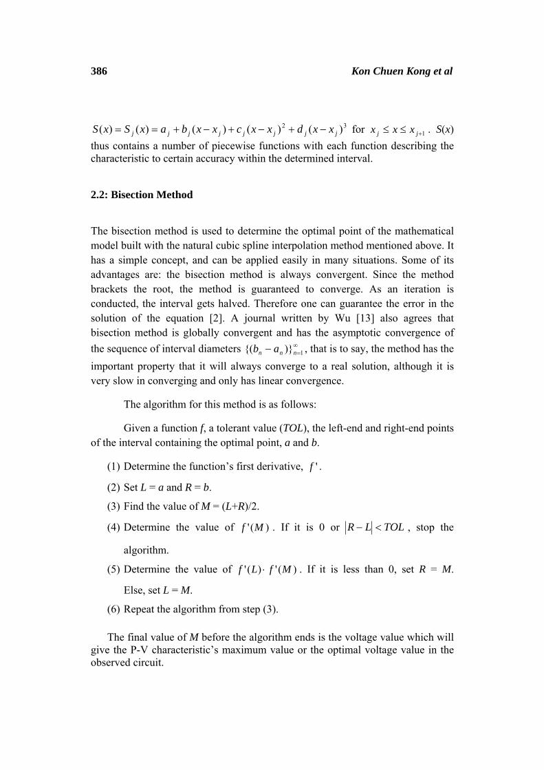
Figure 4. Comparison between simulation data and mathematical model for P-V

characteristic under standard condition.

Through the P-V characteristic’s mathematical model and the use of

bisection method, it is found out that when V = 14.8844 V, the optimal estimated

value for P is obtained, that is 67.4365 W. The optimal value for I is 4.5314 A.

To determine how well a mathematical model’s curve fits the simulation

data, a correlation coefficient can be calculated to determine the goodness-of-fit

between the two curves numerically. The correlation coefficient, denoted r (and

sometimes R), can be determined using the following equation taken from

MathWorld website [4]:

YYXX

XY

SSSSSSr

⋅=

22 . (10)


In (10), X represents one set of data whereas Y contains corresponding data which matches with each data found in X. XYSS is the sum of squared values obtained by multiplying the difference between a data in set X and the mean value of the set with the difference between the corresponding data in Y and the mean value of that set. XXSS and YYSS are obtained by summing each squared value of the difference between a data and the set’s mean value in X and Y, respectively. The value of 2r lies between 0 and 1. The closer the value is to 1, the stronger is the relationship between X and Y.

Tables 1 and 2 represent the sets of data taken from I-V and P-V characteristics, respectively, each containing 20 pairs of corresponding data. The set X represents the data from simulation data, while Y is based on the mathematical model. The mean values for each set is included as well.

V Simulation Data (X) Cubic Spline Model (Y) 1.175 4.8 4.8 2.35 4.8 4.8 3.525 4.799999996 4.8 4.7 4.8 4.8 5.875 4.799999996 4.8 7.05 4.8 4.8 8.225 4.799999956 4.8 9.4 4.799999205 4.7999 10.575 4.799984535 4.800422036 11.75 4.799698837 4.798577425 12.925 4.794265687 4.796552719 14.1 4.719227221 4.7176835 15.275 4.401754334 4.400991993 16.45 3.903277117 3.904637412 17.625 3.331292762 3.330970266 18.8 2.725154503 2.7255248 19.975 2.100042879 2.099889258 21.15 1.463032309 1.46324475 22.325 0.817919089 0.818313688 23.5 0.166955469 0.1670786 Mean: 3.821130195 3.821189322

Table 1. Sets of data taken from I-V characteristics under standard condition


V Simulation Data (X) Cubic Spline Model (Y) 1.175 5.64 5.64 2.35 11.28 11.28 3.525 16.91999999 16.92 4.7 22.56 22.56 5.875 28.19999998 28.19996154 7.05 33.84 33.84002641 8.225 39.47999964 39.48022609 9.4 45.11999253 45.1185 10.575 50.75983646 50.76566249 11.75 56.39646133 56.37850122 12.925 61.965884 62.01312643 14.1 66.54110382 66.5194753 15.275 67.23679745 67.21977992 16.45 64.20890857 64.22911876 17.625 58.71403493 58.70680323 18.8 51.23290466 51.237008 19.975 41.94835651 41.94316484 21.15 30.94313334 30.9490407 22.325 18.26004367 18.26873768 23.5 3.923453531 3.91141 Mean: 38.75854552 38.75902713

Table 2. Sets of data taken from P-V characteristics under standard condition Figures 5 and 6 show the data distribution based on the data sets in Tables 1 and 2.

Figure 5. Distribution of data from Table 1, along with a straight line of X = Y.



From Table 1, 01482347.44=XXSS , 244.0100807=YYSS , and 344.0124461=XYSS . Therefore the correlation coefficient for I-V characteristic,

20.99999973)01008072.44)(01482347.44(

)01244613.44( 22 ==r .

As for the P-V characteristic, calculation based on Table 2 gives 08250.95589=XXSS , 88251.66950=YYSS , and 78251.31064=XYSS , thus

40.99999950)88251.66950)(08250.95589(

)78251.31064( 22 ==r .

Since both values of 2r are very close to 1, it can be said that the model curve fits the simulation data very well, almost the entire line.

Now we consider the conditions of the area surrounding the renewable energy station of UMT. Averaging the data values obtained from 2004 to 2006, we get the values of G = 221.19 W/ 2m , and CT = 28.59 °C. Based on these values, the mathematical model for I-V characteristic is as follows:


(11)

and for P-V:

(12)

The relationship between V, I and P, also the characteristic curves of simulation data and cubic spline model for both I-V and P-V characteristics are shown in Figures 7, 8 and 9:

⎪⎪⎪⎪

⎩

⎪⎪⎪⎪

⎨

⎧

−+−−−−

−−−+−+

−+−−−−

−−−+−+

−+−−−−

=

32

32

32

32

32

)7.20(0155.0)7.20(1067.0)7.20(2215.092.0)4.18(0165.0)4.18(0068.0)4.18(0084.0065.1

)1.16(0013.0)1.16(002.0)1.16(0026.0066.1)8.13(0004.0)8.13(0005.0)8.13(0007.0066.1)5.11(0001.0)5.11(0001.0)5.11(0002.0066.1

066.1

)(

VVVVVV

VVVVVVVVV

VI

237.207.204.184.181.161.168.138.135.11

5.110

≤≤<≤<≤<≤<≤

<≤

VVVVV

V

⎪⎪⎪⎪⎪⎪⎪

⎩

⎪⎪⎪⎪⎪⎪⎪

⎨

⎧

−+−−−−

−−−−−+

−−−+−+

−+−−−+

−−−+−+

−+−−−+

−+−+−+

−+−−−+

=

32

32

32

32

32

32

2

32

)7.20(2151.0)7.20(4845.1)7.20(5577.204.19)4.18(2072.0)4.18(0551.0)4.18(9836.059.19)1.16(0098.0)1.16(0123.0)1.16(0821.1155.17

)8.13(0022.0)8.13(0031.0)8.13(061.1704.14)5.11(0005.0)5.11(0007.0)5.11(0666.1254.12

)2.9(0001.0)2.9(0002.0)2.9(0654.1803.9)9.6(0658.1352.7

)6.4(0002.0)6.4(0654.1901.4)3.2(0001.0)3.2(0002.0)3.2(0654.1451.2

0658.1

)(

VVVVVVVVV

VVVVVV

VVVV

VVVVV

V

VP

237.207.204.184.181.161.168.138.135.11

5.112.92.99.69.66.46.43.2

3.20

≤≤<≤<≤<≤<≤<≤<≤<≤<≤

<≤

VVVVV

VVVV

V


Figure 7. Relationship between I-V and P-V characteristics when G = 221.19

W/ 2m and CT = 28.59 °C.

Figure 8. Comparison between simulation data and mathematical model for I-V

characteristic when G = 221.19 W/ 2m and CT = 28.59 °C.


Figure 9. Comparison between simulation data and mathematical model for P-V

characteristic when G = 221.19 W/ 2m and CT = 28.59 °C.

The bisection method gives the optimal estimation of voltage value, V =

19.5724 V. The matching values of P and I are 20.3335 W and 1.0576 A.

Once again, data are sampled from Figures 8 and 9 to test the goodness-of-

fit. Tables 3 and 4 show the values and means for the sampled data, while Figures

10 and 11 give graphical presentation of their distributions.

V Simulation Data (X) Cubic Spline Model (Y) 1.15 1.065523545 1.066 2.3 1.065523544 1.066 3.45 1.065523544 1.066 4.6 1.065523543 1.066 5.75 1.065523543 1.066 6.9 1.065523542 1.066 8.05 1.065523542 1.066 9.2 1.065523542 1.066 10.35 1.065523541 1.066 11.5 1.065523541 1.066 12.65 1.06552354 1.065789838 13.8 1.065523531 1.066


14.95 1.065523382 1.0668579 16.1 1.065520755 1.066 17.25 1.065474339 1.062342138 18.4 1.064656852 1.065 19.55 1.051068011 1.058558562 20.7 0.919796939 0.92 21.85 0.545704035 0.547737813 23 0.034443262 0.0346955 Mean: 0.979923504 0.980649088

Table 3. Sets of data taken from I-V characteristic when G = 221.19 W/ 2m and CT

= 28.59 °C

V Simulation Data (X) Cubic Spline Model (Y) 1.15 1.225352077 1.22567 2.3 2.450704151 2.451 3.45 3.676056227 3.676097588 4.6 4.901408298 4.901 5.75 6.126760372 6.1264745 6.9 7.35211244 7.352 8.05 8.577464513 8.57767 9.2 9.802816586 9.803 10.35 11.02816865 11.02809759 11.5 12.25352072 12.254 12.65 13.47887278 13.48075531 13.8 14.70422473 14.704 14.95 15.92957456 15.92339618 16.1 17.15488416 17.155 17.25 18.37943235 18.40077718 18.4 19.58968608 19.59 19.55 20.54837962 20.33314495 20.7 19.03979663 19.04 21.85 11.92363317 14.46253396 23 0.792195026 7.9214067 Mean: 10.94675216 11.4203012

Table 4. Sets of data taken from P-V characteristic when G = 221.19 W/ 2m and

CT = 28.59 °C




Mathematical modeling of photovoltaic solar panel 399 For I-V characteristic based on Table 3,

11.20823749=XXSS , 61.20787563=YYSS , and 01.20802440=XYSS ,

so 50.999946772 =r . As for the P-V characteristic,

9776.490437=XXSS , 9685.633458=YYSS , and 2704.645185=XYSS ,

thus 60.932637472 =r . Although both values are not as good as the ones under standard condition, they are still very close to 1, meaning that the model curve fits the simulation data very well in this case study.

4. Conclusion and Discussion In both case studies, built mathematical models fit closely to the simulation

data, and their curves resemble that of a typical I-V and P-V characteristics. The values of 2r calculated from sampled data from each curve also support this observation. However, it is noticeable that the larger error exists near the end in Figure 9, with the largest error having a value close to 6.0476 W. This is due to the reason that the size of subintervals used when building the mathematical models was not small enough, and this has caused S(x) to be unable to give better approximations for intervals where the value of the simulation data changes drastically. The number of decimal places used in calculations might be another factor contributing to the problem occurred. Nevertheless, the value of 2r which is close to 1strongly suggests that the cubic spline model can be accepted as a way to describe the characteristic curve.

By using more subintervals of smaller size and also more decimal places in calculations, it is believed that mathematical models which are able to fit the simulation data better can be built.

Acknowledgment

The authors acknowledge the financial support from Graduate School, Universiti Malaysia Terengganu through SKS.


References

[1] A.K.B. Chand, and M.A. Navascués, Natural bicubic spline fractal interpolation, Nonlinear Anal. 69 (2008), 3679-3691.

[2] Ali Demir, Trisection method by k-Lucas numbers, Appl. Math. Comput. 198 (2008), 339-345.

[3] C.H. Li, X.J. Zhu, G.Y. Cao, S. Sui & M.R. Hu, Dynamic modeling and sizing optimization of stand-alone photovoltaic power systems using hybrid energy storage technology, Renewable Energy 34 (3) (2009), 815-826.

[4] Eric W. Weisstein, Correlation Coefficient, 2010. http://mathworld.wolfram.com/CorrelationCoefficient.html [20 October 2010].

[5] Eric W. Weisstein, Lambert W-function, 2010. http://www.mathworld.wolfram.com/LambertW-function.html [13 April 2010].

[6] G.N. Tiwari, Solar energy: fundamentals, design, modeling and applications, Alpha Science, Pangbourne, 2002.

[7] M.A. Green, Photovoltaic physics and devices, in Gordon, J.M. (ed.) Solar energy: the state of the art: ISES position papers / edited by Jeffery Gordon, International Solar Energy Society, London, 2005, 291-356.

[8] R. Chenni, M. Makhlouf, T. Kerbache and A. Bouzid, A detailed modeling method for photovoltaic cells, Energy 32 (2007), 1724-1730.

[9] REN21 (Renewable Energy and Policy Network for the 21st Century), 2009, Renewables Global Status Report 2009 Update. http://www.ren21.net/pdf/RE_GSR_2009_Update.pdf [8 February 2010].

[10] R.L. Burden, and J.D. Faires, Numerical Analysis, 8th ed., Brooks/Cole, Pacific Grove, CA, 2005.

[11] S.A. Meguid, and M. Al-Dojayli, Accurate modeling of contact using cubic splines, Finite Elements in Analysis and Design 38 (2002), 337-352.

[12] T.C. Banwell, & A. Jayakumar, Exact analytical solution for current flow through diode with series resistance, Electronics Lett. 36 (2000), 291-292.

[13] Xinyuan Wu, Improved Muller method and Bisection method with global and asymptotic superlinear convergence of both point and interval for solving nonlinear equations, Appl. Math. Comput. 166 (2005), 299-311.

Mathematical modeling of photovoltaic solar panel 401 Received: June, 2011

Documents

New Approach on Mathematical Modeling of Photovoltaic ...m-hikari.com/ams/ams-2012/ams-5-8-2012/mamatAMS5-8-2012.pdf · Mathematical modeling of photovoltaic solar panel 387 3. Case