New approach for local C-band weather radar precipitation

© 2021 Universidad Nacional Autónoma de México, Centro de Ciencias de la Atmósfera. This is an open access article under the CC BY-NC License (http://creativecommons.org/licenses/by-nc/4.0/).

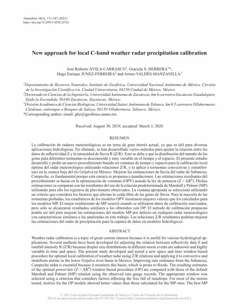
Atmósfera 34(2), 171-187 (2021)https://doi.org/10.20937/ATM.52763

New approach for local C-band weather radar precipitation calibration

José Roberto ÁVILA-CARRASCO1, Graciela S. HERRERA1*, Hugo Enrique JÚNEZ-FERREIRA2 and Arturo VALDÉS-MANZANILLA3

1Departamento de Recursos Naturales, Instituto de Geofísica, Universidad Nacional Autónoma de México, Circuito de la Investigación Científica s/n, Ciudad Universitaria, 04150 Ciudad de México, México.

2Doctorado en Ciencias de la Ingeniería, Universidad Autónoma de Zacatecas, km 6 carretera Zacatecas-Guadalajara, Ejido la Escondida, 98160 Zacatecas, Zacatecas, México.

3División Académica de Ciencias Biológicas, Universidad Juárez Autónoma de Tabasco, km 0.5 carretera Villahermosa-Cárdenas, entronque a Bosques de Saloya, 86150 Villahermosa, Tabasco, México.

*Corresponding author; email: [email protected]

Received: August 30, 2019; accepted: March 3, 2020

RESUMEN

La calibración de radares meteorológicos es un tema de gran interés actual, ya que es útil para diversas aplicaciones hidrológicas. No obstante, se han desarrollado varios métodos para ajustar la relación entre los datos de reflectividad Z y la intensidad de lluvia R (Z/R). Esto se debe a que la distribución del tamaño de las gotas para diferentes tormentas es desconocida y muy variable en el tiempo y el espacio. El presente estudio desarrolló y probó un nuevo procedimiento basado en ventanas de tiempo y espacio para la calibración local óptima del radar meteorológico utilizando relaciones Z/R, y lo aplicó a tormentas convectivas y estratifor-mes en la cuenca baja del río Grijalva en México. Mejorar las estimaciones de lluvia del radar de Sabancuy, Campeche, es fundamental porque esta cuenca es propensa a inundaciones. Las estimaciones resultantes del procedimiento se basan en la optimización de ventanas (OPV) usando la ley de potencia (Z = ARb). Dichas estimaciones se comparan con las resultantes del uso de la relación predeterminada de Marshall y Palmer (MP) utilizando para ello los registros de pluviómetro observados. La ventana apropiada se seleccionó utilizando un criterio que considera los factores que afectan la caída libre de las gotas de lluvia. Para la mayoría de las tormentas probadas, los estadísticos de los modelos OPV mostraron mejores valores que los calculados para los modelos MP. El mejor rendimiento de MP ocurrió cuando se utilizaron datos de calibración suavizados, pero sólo se alcanzaron resultados similares a los obtenidos con OP. El método de calibración propuesto podría ser útil para mejorar las estimaciones del modelo MP por defecto en cualquier radar meteorológico con características similares a las analizadas en este trabajo. Las relaciones Z/R resultantes podrían mejorar las estimaciones del radar de precipitación para la captura de datos en modelos hidrológicos.

ABSTRACT

Weather radar calibration is a topic of great current interest because it is useful for various hydrological ap-plications. Several methods have been developed for adjusting the relation between reflectivity data Z and rainfall intensity R (Z/R) because droplet size distributions in different storm events are unknown and highly variable in time and space. The present study developed and tested a new space and time window-based procedure for optimal local calibration of weather radar using Z/R relations and applying it to convective and stratiform storms in the lower Grijalva river basin in Mexico. Improving rain estimates from the Sabancuy, Campeche radar is essential because it monitors this basin, which is prone to floods. The resulting estimates of the optimal power-law (Z = ARb) window-based procedure (OP) are compared with those of the default Marshall and Palmer (MP) relation using the observed rain gauge records. The appropriate window was selected using a criterion that considers factors affecting the free fall of raindrops. For most of the storms tested, metrics for the OP models showed better values than those calculated for the MP ones. The best MP

172 J. R. Ávila-Carrasco et al.

performance is when using smooth calibration data, achieving similar metric results to that of the OP. The proposed observed calibration method could be useful to improve the default MP model estimates at any weather radar with similar characteristics to the ones analyzed in this work. The resulting Z/R relations could improve precipitation radar estimates for hydrologic model inputs.

Keywords: optimization, flood, power-law, Grijalva river, space-time windows.

1. IntroductionAnalyzing rain gauge information collected within a given basin or region allows understanding the hydrological cycle dynamics, which has a great relevance in socioeconomic, agricultural, and envi-ronmental sectors, among others. Applications range from designing and planning construction projects to predicting extreme events such as droughts and floods (Boushaki et al., 2009). Thus, rainfall information can be considered a basic asset that, like insurance, must be acquired to protect against an uncertain future. Recent developments in computing and Geographic Information Systems (GIS) have allowed distribut-ed hydrological models to increase their popularity among researchers and others interested in the sub-ject, increasing the demand for spatially distributed data in grid format (Mantas et al., 2015). In general, rainfall data is gathered mainly through rain gauge networks, or remote sensing, such as meteorological radars and satellites. These data sources have ad-vantages as well as disadvantages, and differences between them may cause certain grid products to be unsuitable for some applications (Li and Shao, 2010; Woldemeskel et al., 2013).

Rain gauge networks are considered the only source of direct physical measurements of liquid precipitation and, therefore, the most reliable source of information. However, monitoring sites are often scattered and poorly distributed, limited by the spa-tial coverage that prevents their use in hydrological applications. On the other hand, data produced by remote sensors (radar and satellite) represent a potential high-resolution alternative when rain gauge networks are dispersed, especially in poorly monitored regions. Nevertheless, satellite data are indirect measurements that have limitations due to spatio-temporal measurement scales, cloud effects, and the lack of effective algorithms for data recovery (Long et al., 2016).

Weather radar overcomes some rain gauge and sat-ellite data limitations, as they provide high-resolution

raster data with measurements closer to the Earth’s surface than those of satellites. However, radar data re-quire sophisticated post-processing to eliminate some errors such as beam attenuation, bright band effects (Rico-Ramírez et al., 2005), variation in the vertical profile of reflectivity (VPR) (Hill and Baron, 2015), reflectivity attenuation (Gou et al., 2019), non-me-teorological echoes (Dufton and Collier, 2015), and anomalous propagation (Zhang et al., 2019).

Using radar information for environmental and hydrological applications is a topic of great current interest. Since droplet size distributions in different storm events are unknown and vary in time and space, the relationship between reflectivity data Z and rain-fall intensity R (Z/R) is not unique. There are several average empirical Z/R relationships that radars use as default, and the most used expression is based on the empirical study of Marshall and Palmer (1948). However, several researchers and practitioners have developed methodologies that improve those default relationships between reflectivity data Z and rainfall intensity R. The objective is to transform radar re-flectivity (mm6 m–3) into rainfall intensity (mm h–1), adjusting the parameters A and b in a power-law Z/R relation (Z = ARb). This process is commonly known as hydrological radar calibration.

Calheiros and Zawadzki (1987) applied a simple methodology, called the Traditional Matching Meth-od (TMM), that determines the Z/R relationship using regression analysis between two synchronous R and Z data sets in the pixel containing the calibration rain gauge. One disadvantage of this method is that perfect synchronization is only achievable in the ground at the closest distance. The same authors (Calheiros and Zawadzki, 1987) also applied the Probability Matching Method (PMM) to compensate for TMM’s drawbacks. The PMM compares the non-synchro-nous Z and R pairs that have the same cumulative density function.

Window-based methods have proven to be effec-tive, because they allow achieving an optimal Z/R

173Approach for C-Band weather radar calibration

relation by looking for the closest R to Z value with-in a mesh (window) of different spatial and temporal dimensions. Rosenfeld et al. (1994) developed the Window Probability Matching Method (WPMM) to overcome PMM weaknesses by matching Z and R pairs in small space-time windows to account for collocation and timing errors. The WPMM provided significantly better results when estimating rain in-tensity. An advantage of PMM and WPMM is that there are no concurrent requirements for the Z and R data sets. On the other hand, the disadvantages are that these techniques do not represent the actual physical rain process nor use a joint probability for Z and R.

Piman et al. (2007) developed a window-based method, called Window Correlation Matching Method (WCMM), to account for collocation and timing errors. They compared the results with those of the TMM and the WPMM for different scenarios of space-time window sizes, getting the best results using a space window of 7 × 7 km and a time lag of –5 min. The results of the WCMM improved those of the TMM and the PMM, which were overestimated and underestimated, respectively. Yet, for the case study, the WCMM produced a slightly higher rainfall estimation than other methods. However, these au-thors did not consider any specific criterion to select an appropriate window size.

The adjustment of the Z/R relation has been addressed by Alfieri et al. (2010) in the northeast of Italy, readjusting the parameters of the power-law at each time step to find the optimal Z/R relation. The analysis was done for distances less than 25 km from the radar site, comparing rainfall and radar data for 19 rain events. The adjusted Z/R relation produced a 28% reduction of the standard error using a time window of 2 to 5 h compared to the most accurate fixed Z/R relation found in the literature. However, this method did not account for a calibration area away from the radar, nor space windows, only the temporal window.

Ramli and Tahir (2013) in Malaysia developed new Z/R ratios for a Doppler radar using an optimal reflectivity and rain curve for different rainfall types based on their intensity, but this method did not include errors of location or timing. More recently, Ayat et al. (2018) developed the Region Probability Matching Method (RPMM) to calibrate the Amir-

Abad weather radar located in northern Iran. This method overcame the applicability limitations of previous methods in regions with scattered moni-toring, light rains, and poor space-time resolutions. Using 6-h records from 18 synoptic stations and 15 min frequency radar data records, they compared Z/R pairs over the entire radar domain and used the correlation coefficient of a linear model as the cri-terion to adjust the parameters A and b. The results indicate that RPMM was better than TMM; however, this method did not use a power-law Z/R relationship.

In the present study, a new algorithm for a win-dow-based method to find the optimal A and b pow-er-law parameters was developed to ensure the best Z/R relationship. It was tested in the lower Grijalva river basin located between the Mexican states of Tabasco and Chiapas and compared with the perfor-mance of the Marshall and Palmer relation, which is the default method to calculate rainfall intensity in the study area. The region covered in this study is affected by extreme hydrometeorological events that put the population in constant risk (Pedrozo-Acuña et al., 2012), an ideally suited area to develop flood risk management strategies. The main objective of this work is to improve rainfall estimates from the radar installed in the town of Sabancuy, Campeche by finding appropriate local Z/R relations that would increase the reliability of weather-radar rainfall estimations, making them suitable for the critical hydrological applications needed.

2. Study area and dataThe Grijalva river originates in Guatemalan moun-tains and receives different names along its course. Traversing the Mexican states of Chiapas and Tabasco, it flows into the Gulf of Mexico. The Gri-jalva basin is one of the largest in Mexico, and it is divided into three sub-basins: upper, middle, and lower (Hinojosa-Corona et al., 2011). The latter, also called lower Grijalva river basin (LGRB), is within the Grijalva-Usumacinta hydrological region in southeastern Mexico, within the states of Chiapas and Tabasco (Fig. 1). The LGRB covers an area of 23 544 km2 between the geographical coordinates 16º 50’-18º 50’ N and 91º 40’-93º 40’ W, and its maximum elevation is 2892 masl. Elevations within the LGRB are lower than 0 masl, which corresponds


to extensive depressions that remain flooded with fresh water for most of the year (Zavala et al., 2016).

Based on its climate and terrain, the LGRB is subdivided into three regions: (1) highland zone, corresponding to the mountainous region of the basin with elevations ranging from 300 to 2892 masl; (2) transition zone, with elevations ranging from 100 to 300 masl, and (3) lowland zone, with elevations from –20 to 100 masl (Velasco-Martínez et al., 2011). Rainfall is distributed unevenly both in space and time within these three sub-regions, whose climate diversity is present mainly at the highland zone, while it is more homogeneous at the lowland. The maximum rainfall in the LGRB occurs during September, being the transition zone the wettest region with more than 500 mm of monthly rainfall, while in the highland and lowland areas it is around 369 and 360 mm during the same month, respectively. On the other hand, in this basin the most frequent annual rainfall ranges from 1801 to 2200 mm (Velasco-Martínez et al., 2011), which is a much larger value compared to the drier north-ern regions (13-430 mm) or the Mexican national average (700 mm).

2.1 Radar and rain gauge data The National Weather Service (SMN, by its Spanish acronym) of Mexico operates a network of 13 weath-er radars, most of them in southern Mexico. Two ra-dars partially cover the LGRB, located in the towns of Sabancuy in Campeche and Mozotal in Chiapas. The latter is located at 2900 masl and only covers the upper part of the GLRB. The Sabancuy radar (Fig. 2), which covers all the physio-climatic regions of the basin, is located at 18º 58’ 20.784’’ N and 91º 10’ 21.5904’’ W at only 17 masl (5 m of land plus a 12 m tower). Installed in 2012, the Sabancuy radar is a dual-polarized Doppler type with a coaxial mag-netron, operating in the type C-band (wavelength λ = 5 cm and frequency of 4-8 GHz). Dual polar-ization means better estimation and hydrometeor classification (like hail and rain) in quantitative rainfall calculation.

Dual polarization type C-band radars are pref-erable than single polarization type S-band radars (λ = 10 cm) because they are less expensive and bulky, they allow precise real-time correction of beam attenuation and they provide similar accuracy to sin-gle-polarization type S-band radars. Table I presents

Fig. 1. Spatial location, hydrography, urban areas, and topography of the lower Gri-jalva river basin.

18º3

0'0'

'N17

º30'

0''N

18º0

'0''N

17º0

'0''N

18º3

0'0'

'N17

º30'

0''N

18º0

'0''N

17º0

'0''N

93º30'0''W 92º30'0''W 91º30'0''W93º0'0''W 92º0'0''W 91º0'0''W

93º30'0''W 92º30'0''W 91º30'0''W93º0'0''W 92º0'0''W 91º0'0''W

0 10 20 40 60

Kilometers

SymbologyRiversUrban Zone

Elevation (masl)

Smaller than 00 - 5050 - 100100 - 300300 - 600600 - 10001000 - 15001500 - 20002000 - 2400Greater than 2400

LOWER GRIJALVA RIVER BASIN


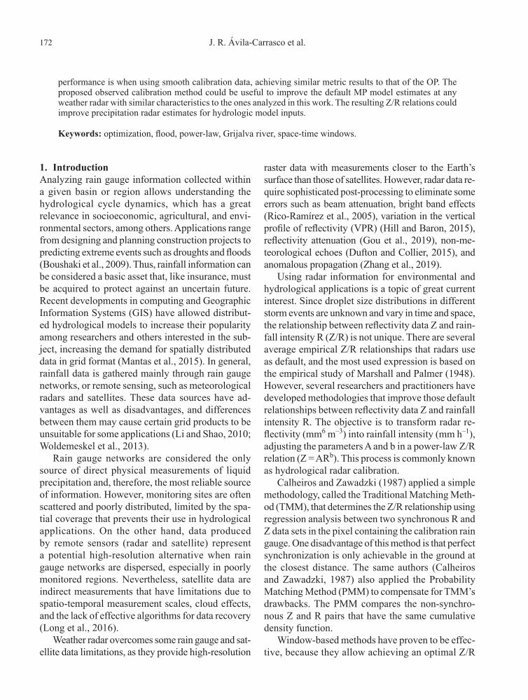
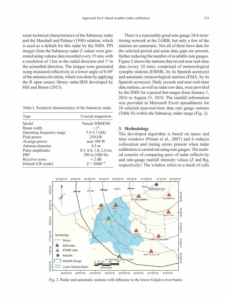
some technical characteristics of the Sabancuy radar and the Marshall and Palmer (1948) relation, which is used as a default for this radar by the SMN. PPI images from the Sabancuy radar Z values were gen-erated using volume data recorded every 15 min, with a resolution of 1 km in the radial direction and 1º in the azimuthal direction. The images were generated using measured reflectivity at a lower angle of 0.49º of the antenna elevation, which was done by applying the R open source library radar.IRIS developed by Hill and Baron (2015).

There is a reasonably good rain-gauge 24-h mon-itoring network at the LGRB, but only a few of the stations are automatic. Not all of them have data for the selected period and some data gaps are present, further reducing the number of available rain gauges. Figure 2 shows the stations that record near real-time data (every 10 min), comprised of meteorological synoptic stations (ESIME, by its Spanish acronym) and automatic meteorological stations (EMA, by its Spanish acronym). Daily records and near-real-time data stations, as well as radar raw data, were provided by the SMN for a period that ranges from January 1, 2016 to August 31, 2018. The rainfall information was provided in Microsoft Excel spreadsheets for 10 selected near-real-time data rain gauge stations (Table II) within the Sabancuy radar range (Fig. 2).

3. MethodologyThe developed algorithm is based on space and time windows (Piman et al., 2007) and it reduces collocation and timing errors present when radar calibration is carried out using rain gauges. The meth-od consists of comparing pairs of radar reflectivity and rain-gauge rainfall intensity values (Z and Rg, respectively). The window refers to a mesh of cells

Table I. Technical characteristics of the Sabancuy radar.

Type Coaxial magnetron

Model Vaisala WRM200Beam width < 1ºOperating frequency range 5.5-5.7 GHzPeak power 250 kWAverage power max 300 WAntenna diameter 4.5 mPulse amplitudes 0.5, 0.8, 1.0, 2.0 msPRF 200 to 2400 HzReceiver noise < 2 dBDefault Z/R model Z = 200R1.6

94º30'0''W 93º30'0''W 92º30'0''W 91º30'0''W 90º30'0''W93º0'0''W94º0'0''W 92º0'0''W 91º0'0''W

94º30'0''W 93º30'0''W 92º30'0''W 91º30'0''W93º0'0''W94º0'0''W 92º0'0''W 91º0'0''W

18º3

0'0'

'N17

º30'

0''N

16º3

0'0'

'N18

º0'0

''N19

º0'0

''N17

º0'0

''N

18º3

0'0'

'N17

º30'

0''N

16º3

0'0'

'N18

º0'0

''N17

º0'0

''NRivers

RADAR

RADAR Range

Lower Grijalva Basin

EMA dataESIME data

Symbology

0 15 30

Kilometers

60 90

Fig. 2. Radar and automatic stations with influence in the lower Grijalva river basin.


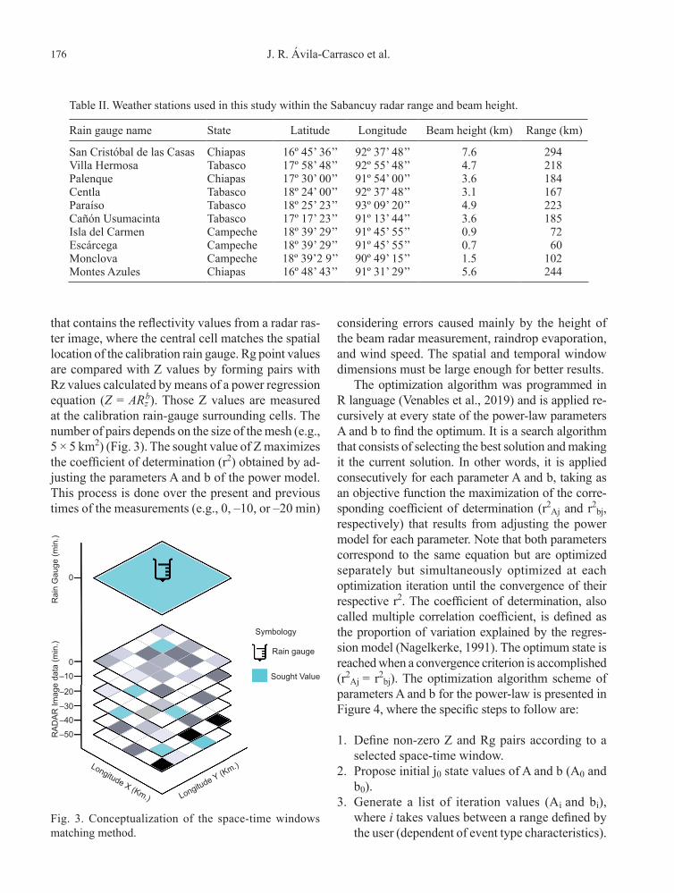
that contains the reflectivity values from a radar ras-ter image, where the central cell matches the spatial location of the calibration rain gauge. Rg point values are compared with Z values by forming pairs with Rz values calculated by means of a power regression equation (Z = ARz

b). Those Z values are measured at the calibration rain-gauge surrounding cells. The number of pairs depends on the size of the mesh (e.g., 5 × 5 km2) (Fig. 3). The sought value of Z maximizes the coefficient of determination (r2) obtained by ad-justing the parameters A and b of the power model. This process is done over the present and previous times of the measurements (e.g., 0, –10, or –20 min)

considering errors caused mainly by the height of the beam radar measurement, raindrop evaporation, and wind speed. The spatial and temporal window dimensions must be large enough for better results.

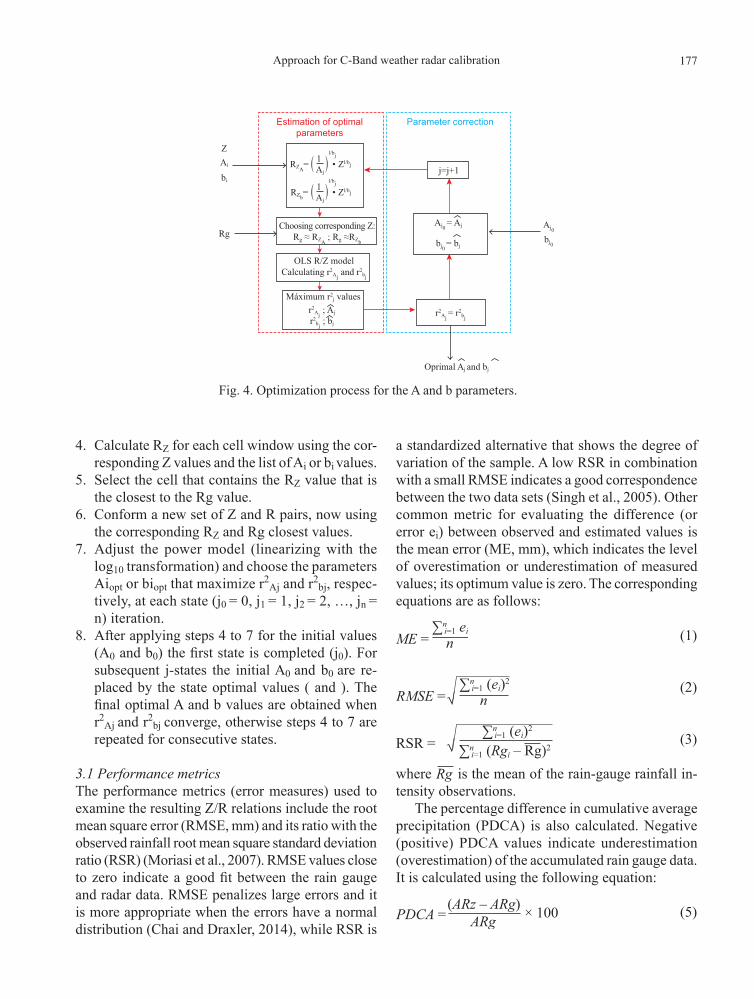
The optimization algorithm was programmed in R language (Venables et al., 2019) and is applied re-cursively at every state of the power-law parameters A and b to find the optimum. It is a search algorithm that consists of selecting the best solution and making it the current solution. In other words, it is applied consecutively for each parameter A and b, taking as an objective function the maximization of the corre-sponding coefficient of determination (r2

Aj and r2bj,

respectively) that results from adjusting the power model for each parameter. Note that both parameters correspond to the same equation but are optimized separately but simultaneously optimized at each optimization iteration until the convergence of their respective r2. The coefficient of determination, also called multiple correlation coefficient, is defined as the proportion of variation explained by the regres-sion model (Nagelkerke, 1991). The optimum state is reached when a convergence criterion is accomplished (r2

Aj = r2bj). The optimization algorithm scheme of

parameters A and b for the power-law is presented in Figure 4, where the specific steps to follow are:

1. Define non-zero Z and Rg pairs according to a selected space-time window.

2. Propose initial j0 state values of A and b (A0 and b0).

3. Generate a list of iteration values (Ai and bi), where i takes values between a range defined by the user (dependent of event type characteristics).

0

0

–10

–20

–30

–40

–50

Longitude X (Km.) Longitude Y (Km.)

RA

DA

R Im

age

data

(min

.)R

ain

Gau

ge (m

in.)

Symbology

Rain gauge

Sought Value

Fig. 3. Conceptualization of the space-time windows matching method.

Table II. Weather stations used in this study within the Sabancuy radar range and beam height.

Rain gauge name State Latitude Longitude Beam height (km) Range (km)

San Cristóbal de las Casas Chiapas 16º 45’ 36’’ 92º 37’ 48’’ 7.6 294Villa Hermosa Tabasco 17º 58’ 48’’ 92º 55’ 48’’ 4.7 218Palenque Chiapas 17º 30’ 00’’ 91º 54’ 00’’ 3.6 184Centla Tabasco 18º 24’ 00’’ 92º 37’ 48’’ 3.1 167Paraíso Tabasco 18º 25’ 23’’ 93º 09’ 20’’ 4.9 223Cañón Usumacinta Tabasco 17º 17’ 23’’ 91º 13’ 44’’ 3.6 185Isla del Carmen Campeche 18º 39’ 29’’ 91º 45’ 55’’ 0.9 72Escárcega Campeche 18º 39’ 29’’ 91º 45’ 55’’ 0.7 60Monclova Campeche 18º 39’2 9’’ 90º 49’ 15’’ 1.5 102Montes Azules Chiapas 16º 48’ 43’’ 91º 31’ 29’’ 5.6 244


4. Calculate RZ for each cell window using the cor-responding Z values and the list of Ai or bi values.

5. Select the cell that contains the RZ value that is the closest to the Rg value.

6. Conform a new set of Z and R pairs, now using the corresponding RZ and Rg closest values.

7. Adjust the power model (linearizing with the log10 transformation) and choose the parameters Aiopt or biopt that maximize r2

Aj and r2bj, respec-

tively, at each state (j0 = 0, j1 = 1, j2 = 2, …, jn = n) iteration.

8. After applying steps 4 to 7 for the initial values (A0 and b0) the first state is completed (j0). For subsequent j-states the initial A0 and b0 are re-placed by the state optimal values ( and ). The final optimal A and b values are obtained when r2

Aj and r2bj converge, otherwise steps 4 to 7 are

repeated for consecutive states.

3.1 Performance metricsThe performance metrics (error measures) used to examine the resulting Z/R relations include the root mean square error (RMSE, mm) and its ratio with the observed rainfall root mean square standard deviation ratio (RSR) (Moriasi et al., 2007). RMSE values close to zero indicate a good fit between the rain gauge and radar data. RMSE penalizes large errors and it is more appropriate when the errors have a normal distribution (Chai and Draxler, 2014), while RSR is

a standardized alternative that shows the degree of variation of the sample. A low RSR in combination with a small RMSE indicates a good correspondence between the two data sets (Singh et al., 2005). Other common metric for evaluating the difference (or error ei) between observed and estimated values is the mean error (ME, mm), which indicates the level of overestimation or underestimation of measured values; its optimum value is zero. The corresponding equations are as follows:

ME =∑n

i=1 ein (1)

RMSE =∑n

i=1 (ei)2

n√ (2)

RSR =∑ni=1 (ei)2

∑ni=1 (Rgi – Rg)2√ (3)

where Rg is the mean of the rain-gauge rainfall in-tensity observations.

The percentage difference in cumulative average precipitation (PDCA) is also calculated. Negative (positive) PDCA values indicate underestimation (overestimation) of the accumulated rain gauge data. It is calculated using the following equation:

PDCA = × 100(ARz – ARg)ARg (5)

Estimation of optimalparameters

Parameter correction

Z

Rg

j=j+1

bj0

Aj0

Oprimal Aj and bj

Ai

bi

Aj0 = Aj

r2Aj

= r2bj

r2Aj

; Aj

r2bj

; bj

Máximum r2j values

OLS R/Z modelCalculating r2

Aj and r2

bj

Choosing corresponding Z:Rg ≈ RZA

; Rg ≈RZb bj0 = bj

RZA= ( ) Zl/bj•1

Aj

l/bj

RZb= ( ) Zl/bj•1

Aj

l/bj

Fig. 4. Optimization process for the A and b parameters.


where ARα, α = z or g, is the cumulative precipitation of the corresponding data source. The relation be-tween radar and rain gauge data is not linear, and in general the power-law of the form Z = ARb gives the best fit of the data (Brase and Brase, 2009). Thus, to find the correlation between these two types of data, a power-type mathematical regression model should be adjusted (Newman, 2005). The power-law equation is linearized applying a logarithmic transformation: log Z = log A + b log R.

It is possible to calculate the correlation expressed as the coefficient of determination (r2) from the adjust-ed least-squares line. The correlation varies from 0 to 1 and indicates the model goodness of fit. It defines the proportion of the variance of the measured rainfall that is explained by the regression model. Values of r2 > 0.5 are considered acceptable, while r2 = 1 indicates a perfect correlation, but r2 = 0 reveals that the mean is a better predictor than the model, which is unacceptable. The equation for r2 between the radar rain estimates (E) and the rain gauge observed values (O) is given by the following equation:

r2 =(n ∑ OiEi – ∑ Oi ∑ Ei)2

[(n ∑ Oi2 – (∑ Oi)2][(n ∑ Ei

2 – (∑ Ei)2] (6)

It is also important to apply criteria to reasonably determine window dimensions of space and time. Calheiros and Zawadzki (1987) proposed a relation-ship to compare different spatiotemporal distributions of these two types of data sources, assuming that the temporal resolution of rainfall data should be equiva-lent to the spatial resolution of radar data. Taking into account rainfall statistical properties this relationship is given by the following equation:

1.3√Ar = vt → Ar = tv1.3( ) (7)

where Ar is the area of the radar data, t is the temporal resolution of rain gauge data, and v is the translation speed of the precipitation cells. An alternative is to use the kinematic equation of semi-parabolic motion to find the distance at which a raindrop is advected by the wind. This expression is x = v t, so the distance (x in meters) is equal to the product of the wind speed (v in ms–1) in the time (t in seconds) that the falling raindrop takes to reach the ground.

4. Results and discussionThe methodology was tested in a total of seven storms, covering both stratiform and convective cases that occurred in winter and summer (Table III). In general, the stratiform-type storms have more compact spatial and temporal distributions com-pared with convective ones. Radar calibration for each of the storm events is performed by means of near real-time stations with data records taken every 10 min. Rainfall data values occur uneven at each position so that the number of Z/R pairs at each re-cording time was variable. Note also that null records were removed, further reducing the number of Z/R pairs. Rain gauge stations installed on the towns of Villahermosa, Centla, Isla del Carmen, Paraíso, and Escárcega had a larger number of data for the period of interest. To compare both data sources at the same frequency with the largest number of pairs possible, the Sabancuy radar records were interpolated to a 10 min frequency using the two adjacent temporal measurements.

Table III. Storm events analyzed.

Date Start(LT)

End(LT)

Duration(h)

Precipitation (mm)*

Mean intensity (mm/h)

Storm event type

01/02/2016 9: 30 23:00 13:30 86.00 6.37 Stratiform20/07/2016 3:00 9:30 6:30 39 6.15 Convective16/02/2017 8:30 12:00 3:30 21.00 6.00 Stratiform29/01/2017 11:00 18:30 7:30 25.6 3.41 Stratiform13/02/2018 5:00 7:45 2:45 28.00 10.18 Convective14/02/2018 2:00 5:15 3:15 68.25 21.00 Convective04/06/2018 20:45 0:00 3:15 48.40 14.89 Convective

*Maximum accumulated rainfall recorded in one specific rain gauge.


For stratiform events, the iteration values were selected within the 0-100 range with increments of 1 for parameter A, while for parameter b they were selected within the 0-5 range with increments of 0.1. For convective events, to get an appropriate curve shape, the iteration ranges were twice as large as for the stratiform case (0 to 200 for A and 0 to 10 for b) with the same increments as before for both param-eters. The lists of iteration values are used initially in the optimization process, then the increments are reduced, and in consequence, the number of iteration values increased.

Table IV shows the resulting r2 (= r2A =r2

b) val-ues and parameters A and b, for the stratiform event observed on 29/01/2017, for each spatiotemporal window tested. The corresponding results for the convective event observed on 20/07/2016 is shown in Table V. For the stratiform event (Table IV), an r2 = 0.34 can be observed for the 3 × 3 km2 window time (0 min).

Better values for r2 resulted at –10 min, which is evident from the 3 × 3 to 9 × 9 km2, where an r2 of 0.9 was reached. Beyond –10 min, improvements are observed at –20 min with r2 = 0.96 for the 15 × 15 km2 window, and –30 min for the 17 × 17 km window with r2 = 0.98, which is almost a perfect correlation. Correlations above 0.9 are considered excellent. Similar results were obtained by Piman et al. (2007), who reported an increase in the correlation value for both the time and space-time scales. This is to be expected, since the more pixels are considered the higher the chances of finding values Rz closer to Rg values.

The performance of the optimization algorithm for the convective storm event was different, resulting in parameter values larger than those for the stratiform event. One possible reason is that summer rainstorms generally occur as showers, and differences among measurements at climate stations are larger (Ducrocq et al., 2002), hence they are more difficult to estimate

Table IV. Optimal parameter model results of the 29/01/2017 stratiform storm event.

Spatial window (km2)

Temporal window (min)

0 –10 –20 –30 –40

A b r2 A b r2 A b r2 A b r2 A b r2

3 × 3 10.6 1 0.34 6.0 2.4 0.37 2.0 2.9 0.22 1.0 3.9 0.23 1 3.5 0.115 × 5 6.7 1.74 0.53 11.0 1.7 0.62 6.0 1.8 0.37 2.0 2.9 0.25 1 3.6 0.217 × 7 11.9 1.39 0.71 11.0 1.6 0.8 12.0 1.4 0.6 3.0 2.7 0.4 2 2.8 0.389 × 9 19.3 1 0.85 17.8 1.1 0.9 14.1 1.2 0.76 19.0 1.3 0.55 19 1.6 0.5815 × 15 22 1 0.95 11.0 1.1 0.96 8.0 1.3 0.96 13.0 0.9 0.93 20 0.7 0.917 × 17 31 0.5 0.97 17.0 0.8 0.97 6.0 1.3 0.96 14.0 0.6 0.98 25 0.6 0.9619 × 19 35 0.4 0.99 14.0 0.8 0.98 13.0 0.7 0.99 14.0 0.4 0.99 29 0.4 0.99

Table V. Optimal parameter model results of the 20/07/2016 convective storm event.

Spatial window (km2)

Temporal window (min)

0 –10 –20 –30 –40

A b r2 A b r2 A b r2 A b r2 A b r2

3 × 3 7 3.4 0.22 5 3.6 0.21 3 4.2 0.17 1 4.5 0.11 1 4.9 0.15 × 5 24 2.8 0.27 12 3.4 0.39 6 3.8 0.3 3 4.2 0.21 3 4.1 0.27 × 7 63 2.4 0.37 24 3.6 0.37 10 4.7 0.18 1 5 0.06 1 6.5 0.059 × 9 36.3 2.56 0.43 30.2 2.71 0.63 19 3.1 0.48 8 3.5 0.38 7 3.4 0.34

15 × 15 74 2 0.64 65 2.4 0.72 34 2.8 0.44 12 3.8 0.24 3 4.8 0.17617 × 17 68 1.9 0.82 55 2.2 0.84 25 2.7 0.7 15 2.9 0.58 9 3 0.5219 × 19 72 1.8 0.86 71 1.9 0.88 34 2.3 0.76 15 2.6 0.63 10 2.8 0.56


using smaller windows (Junker et al., 2002). The r2 value improved when increasing the window size, but the number of stations used for calibration also had an impact.

This result is similar to that obtained by Hakvoort et al. (1993), who noted that increasing the number of rain gauges improved the model adjustment, but not as much as their placement; however, they did not differentiate between types of events. On the other hand, Lane et al. (1998) emphasized that a low-density rain gauge network (with separations of 5-20 km) could be sufficient to obtain a good precip-itation estimate for stratiform events because these could occur homogeneously in space and time. That is not the case for convective events, because tempo-ral Z rate changes are larger and storm cores could be undetected between rain gauges. In the –10 min temporal windows, an r2 improvement can be observed for all spatial windows except for 3 × 3 and 5 × 5 km2 (Table V). Note that an r2 of 0.9 is not obtained, suggesting that further window expansion is required.

Once r2 values for each spatial and temporal win-dow were obtained, the question is which of these should be chosen to get the final estimates. The ad-equate window size was chosen using physical laws that answer the following question: Which is the maximum distance raindrops would be advected by the wind dragged a certain time period? Two alter-natives were considered: (1) to apply the kinematic equation, and (2) to apply the equation proposed by Calheiros and Zawadzki (1987). The time t that a raindrop takes to reach the ground was defined as 10 min, given the good r2 results obtained for this time-window, and a mean speed v of 25 km h–1 (~ 7m s–1), calculated from the analyzed storms, was chosen. The kinematic equation, disregarding the weight of the drops, results in:

Distance = (7 m s–1) (600 s) = 4.2 km (8)

corresponding to a radius in which the raindrops could fall and suggesting the selection of a 9 × 9 km2 space and a –10 min window, respectively.

Equation 9 shows the results using Calheiros and Zawadzki (1987) method:

Area = = 10.97 km20.166 h x 25 km h–1

1.3 (9)

The result suggests using a window between 3 × 3 and 4 × 4 km2. Care should be taken in selecting the wind speed, since for very strong storms this value would be much larger. For example, for tropical storms it would exceed 90 km h–1, and for hurricanes it would range between 120 to 300 km h–1. The ele-vation error related to the Earth curvature should be considered as well, because for a distance of 200 km and an angle of 0.5º it will be 4 km (Gao et al., 2006).

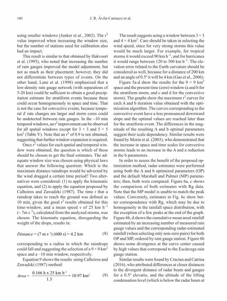
Figure 5a-d show the results for the 9 × 9 km2 space and the present time (zero) window (a and b for the stratiform storm, and c and d for the convective storm). The graphs show the maximum r2 curves for each A and b iteration value obtained with the opti-mization algorithm. The curves corresponding to the convective event have a less pronounced downward slope and the optimal values are reached later than for the stratiform event. The differences in the mag-nitude of the resulting A and b optimal parameters suggest their scale dependency. Similar results were found by Morin et al. (2003), who demonstrated that the increase in space and time scales for convective storms leads to an increase in the A and a reduction in the b parameters.

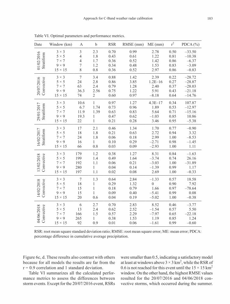
In order to assess the benefit of the proposed op-timization method, radar estimates were performed using both the A and b optimized parameters (OP) and the default Marshall and Palmer (MP) parame-ters; then, both were compared. Figure 6a, c shows the comparison of both estimates with Rg data. Note that the MP model is unable to match the peak values. Conversely, estimates in Fig. 6c show bet-ter correspondence with Rg, which may be due to homogeneity in the rainfall space distribution, with the exception of a few peaks at the end of the graph. Figure 6b, d shows the cumulative mean areal rainfall estimated by an increasing number of measured rain gauge values and the corresponding radar-estimated rainfall (when selecting only non-zero pairs) for both OP and MP, ordered by rain gauge station. Figure 6b shows some divergence at the curve center caused by high values that correspond to the Escárcega rain gauge station.

Similar results were found by Craciun and Catrina (2016), who attributed differences at closer distances to the divergent distance of radar beam and gauges for a 0.5º elevatio, and the altitude of the lifting condensation level (which is below the radar beam at


long distances but higher at closer distances. Another possible reason for this radar overestimation is the remnant ground clutter echoes, and systematic and collecting data errors present at the rain gauge station are not ruled out. There is also a slight overestimation at the end of the curve at data pairs corresponding to the Villahermosa rain gauge station. Because this is the most distant station from the Sabancuy radar, errors are likely related to radar beam elevation, rain-drop evaporation, signal attenuation, and systematic radar errors. The accumulated curve plot for the convective event (Fig. 6d) also shows a divergence in the center, but this is not very pronounced. The maximum separation occurs at the end of the curve due to the occurring peak values in this part.

The corresponding PDCA values (Table VI) were –21 and 10% using the OP model for convective and stratiform events, respectively. The negative PDCA value for the convective event means that rain gauge

values were mainly overestimated by the OP model; the opposite occurs for the stratiform events. The resultant PDCA for the MP model shows that values are underestimated for both events with –18.7 and –68.3%, respectively. The percentages obtained using the OP model in both storm events are considered acceptable given the recorded rainfall magnitudes, but the resulting PDCA using the MP model for the convective is also high.

Scattergrams in Figure 7a, b show the estimated radar rainfall data vs. calibration rain-gauge values (in millimeters). Although the optimization algorithm computes r2 using the power-law linearized equation, the purpose of these graphs is to compare rain gauge observed values with those estimated by the radar data. The scattergrams show that the power model gave better r2 values than the linear model, yet the r2 difference between both models was small (not shown). Figure 7b shows greater dispersion and a

Stratiform Event (2017/01/29)

a) b)

c) d)

Parameter A

0.1

0

0 20 40 60 80 100 120 140 160 180 200

10 20 30 40 50 60 70 80 90 100 0.0 0.5 1.0 1.5 2.0 2.5 3.0 3.5 4.0 4.5 5.0

0.2

0.3

0.4

0.5

0.6

0.7

0.8

Parameter A

Stratiform Event (2017/01/29)Parameter b

0.1

0.2

0.3

0.4

0.5

0.6

0.7

0.8

Parameter b

Convective Event (2016/07/20)Parameter A

0.1

0.2

0.3

0.4

0.5

0.6

Parameter A0 20 40 60 80 100 120 140 160 180 200

Parameter A

Convective Event (2016/07/20)Parameter A

0.1

0.2

0.3

0.4

0.5

0.6

Coe

ffici

ent o

f Det

erm

inat

ion

(r2 )

Coe

ffici

ent o

f Det

erm

inat

ion

(r2 )

Coe

ffici

ent o

f Det

erm

inat

ion

(r2 )

Coe

ffici

ent o

f Det

erm

inat

ion

(r2 )

Fig. 5. Parameters A and b vs. r2 curves for (a, b) stratiform and (c, d) convective storm events. The maximum value in each curve corresponds to the optimal parameters: A=19.3, b= 1 for the stratiform event, and A =36.3, b=2.56 for the convective event.


smaller r2 values than Figure 7a (0.69 < 0.86), which indicates that the convective storm has a higher complexity than the stratiform one. Nevertheless, the convective storm accumulated curve seems to fit data better than the stratiform curve. One reason may be the scale differences of each event, since the total accumulated rain for the stratiform event does not exceed 50 mm, while in the convective event it was more than 140 mm. Additionally, there are more Z/R pairs with differences in the convective event, which result in a greater PDCA value.

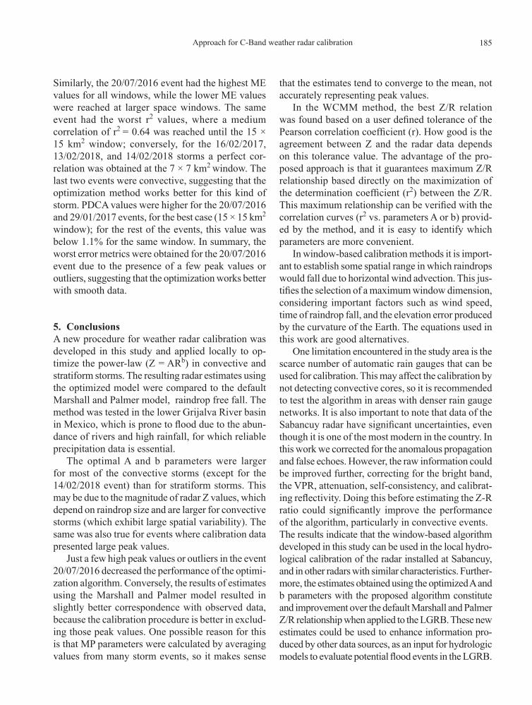
The level of agreement for the rest of the storm events can be assessed using the Taylor diagram for the windows 3 × 3 to 15 × 15 km2 at time zero (Fig. 8). The azimuth shows the correlation (r) between each tested window models and the observed data, while the radial distance measures the standard deviation (SD). The black hollow circle indicates correlation and standard deviation of the observed

rain gauge data, and the other symbols indicate the tested window models. The closest the symbols are to the black hollow dot, the better the correspon-dence between the different window models with the rain gauge data.

The diagrams clearly show the advantage of using the optimized A and b parameters (filled symbols), instead of the default Marshall and Palmer parameters (hollow symbols). In almost all cases the filled symbols perform better than their hollow counterparts; this is more evident for the 2016/02/01, 2017/01/29, and 2018/02/13-14 storm events. For the 2017/02/16 and 2018/06/04 events, results for both the OP and MP approaches show good correlations (> 0.7) are observed in both events, especially in 2017/02/16. The 2016/07/20 storm event is the only one where MP results seems to be slightly better than those using OP parameters, but this difference is very subtle as can be seen in

0000 55 1010 1515 2020 2525 3030 3535 4040 4545 5050

11

22

33

44

55

66

Rg − Rz Pairs Rg − Rz Pairs

Rai

nfal

l (m

m)

Rai

nfal

l (m

m)

Rai

nfal

l (m

m)

Rai

nfal

l (m

m)

DataDataMPMPOPOPRGRG

Rainfall (2017/01/29)Rainfall (2017/01/29)

00

1010

2020

3030

4040

5050

Acc

umul

ated

Rai

nfal

l (m

m)

Acc

umul

ated

Rai

nfal

l (m

m)


Accumulated Rainfall (2017/01/29)Accumulated Rainfall (2017/01/29)

0000 1010 2020 3030 4040 5050 6060 7070 8080 9090 100100 110110

22

44

66

88

1010 DataDataMPMPOPOPRGRG

Rainfall (2016/07/20)Rainfall (2016/07/20)c)c) d)d)

a)a) b)b)

00

2020

4040

6060

8080

100100

120120

140140

Acc

umul

ated

Rai

nfal

l (m

m)

Acc

umul

ated

Rai

nfal

l (m

m)


Accumulated Rainfall (2016/07/20)Accumulated Rainfall (2016/07/20)

Rg − Rz Pairs Rg − Rz Pairs 00 1010 2020 3030 4040 5050 6060 7070 8080 9090 100100 110110

Rg − Rz Pairs Rg − Rz Pairs

00 55 1010 1515 2020 2525 3030 3535 4040 4545 5050Rg − Rz Pairs Rg − Rz Pairs

Fig. 6. Comparison by number of pairs of observed (Rg) values and estimated values using optimized A and b parameters (OP) and the Marshall and Palmer default parameters (MP). (a) Value by value series of Rg vs. OP and MP for the 2017/01/29 event; (b) acummulated rainfall curve of Rg vs. OP and MP for the 2017/01/29 event; (c) value by value series of Rg vs. OP and MP for the 2016/07/20 event; (d) acummulated rainfall curve of Rg vs. OP and MP for the 2016/07/20 event.


Figure 6c, d. These results also contrast with others because for all models the results are far from the r = 0.9 correlation and 1 standard deviation.

Table VI summarizes all the calculated perfor-mance metrics to assess the differences between storm events. Except for the 20/07/2016 event, RSRs

were smaller than 0.5, indicating a satisfactory model at least at windows above 3 × 3 km2, while the RSR of 0.6 is not reached for this event until the 15 × 15 km2 window. On the other hand, the highest RMSE values resulted for the 20/07/2016 and 04/06/2018 con-vective storms, which occurred during the summer.

Table VI. Optimal parameters and performance metrics.

Date Window (km) A b RSR RMSE (mm) ME (mm) r2 PDCA (%)01

/02/

2016

Stra

tifor

m 3 × 3 3 2.3 0.70 0.99 2.78 0.50 –33.505 × 5 4 1.8 0.43 0.61 1.22 0.81 –10.387 × 7 4 1.7 0.36 0.52 1.42 0.86 –6.379 × 9 7 1.2 0.34 0.48 1.53 0.83 –3.09

15 × 15 8 0.8 0.36 0.52 2.97 0.86 –0.83

20/0

7/20

16C

onve

ctiv

e 3 × 3 7 3.4 0.88 1.42 2.39 0.22 –28.725 × 5 24 2.8 0.86 3.85 1.2E–16 0.27 –28.877 × 7 63 2.4 0.79 1.28 2.40 0.37 –28.039 × 9 36.3 2.56 0.75 1.22 5.91 0.43 –21.18

15 × 15 74 2 0.60 0.97 –8.18 0.64 –14.76

29/0

1/20

17St

ratif

orm 3 × 3 10.6 1 0.97 1.27 4.3E–17 0.34 107.87

5 × 5 6.7 1.74 0.73 0.96 1.89 0.53 –12.977 × 7 11.9 1.39 0.63 0.83 5.64 0.71 –15.169 × 9 19.3 1 0.47 0.62 –1.03 0.85 10.86

15 × 15 22 1 0.21 0.28 3.46 0.95 –5.38

16/0

2/20

17St

ratif

orm 3 × 3 17 2.1 0.46 1.34 1.70 0.77 –0.90

5 × 5 18 1.8 0.21 0.63 2.72 0.94 3.327 × 7 24 1.8 0.06 0.18 2.99 1.00 –8.539 × 9 16 1 0.10 0.29 –2.71 0.98 –1.45

15 × 15 66 0.8 0.03 0.09 –2.93 1.00 1.11

13/0

2/20

18C

onve

ctiv

e 3 × 3 179 1.2 0.38 1.27 8.31 0.84 –1.635 × 5 199 1.4 0.49 1.64 –3.74 0.74 26.167 × 7 192 1.1 0.06 0.21 –3.03 1.00 –31.899 × 9 280 1 0.04 0.14 –1.39 0.99 1.17

15 × 15 197 1.1 0.02 0.08 2.69 1.00 –0.33

14/0

2/20

18C

onve

ctiv

e 3 × 3 7 1.3 0.64 2.84 –1.33 0.57 18.585 × 5 18 1 0.29 1.32 0 0.90 7.927 × 7 15 1 0.18 0.79 1.66 0.97 –78.649 × 9 15 1 0.09 0.40 –5.41 0.99 0.08

15 × 15 20 0.6 0.04 0.19 –5.02 1.00 –0.38

04/0

6/20

18C

onve

ctiv

e 3 × 3 6 2.7 0.70 2.83 8.52 0.46 –3.775 × 5 13 2.4 0.62 2.52 –1.54 0.57 5.507 × 7 166 1.5 0.57 2.29 –7.97 0.65 –22.189 × 9 265 1 0.38 1.53 1.19 0.85 1.24

15 × 15 92 0.9 0.01 0.06 –1.61 0.99 –0.60

RSR: root mean square standard deviation ratio; RMSE: root mean square error; ME: mean error; PDCA: percentage difference in cumulative average precipitation.


2.0

3.0

4.0

5.0

6.0

RA

DA

R (m

m)

Stratiform Event (2017/01/29)a) b)

y = 0.8963x0.859

R² = 0.86030.0

0 1 2 3 4 5 6 7 0 1 2 3 4 5 6 7 8 9 10 11 12

1.0

Rain Gauge (mm)

2.01.5

2.53.03.54.04.55.0

RA

DA

R (m

m)

Convective Event (2016/07/20)

y = 0.8728x0.69

R² = 0.69450.00.51.0

Rain Gauge (mm)

Fig. 7. Scatter diagrams of Rz-Rg values (mm), for (a) stratiform and (b) convective storm events.

Fig. 8. Taylor diagrams for different space windows from 3 × 3 to 15 × 15 km2 at time zero for all storm events. The hollow symbols indicate results (of SD and r) calculated using the Marshall and Palmer default model (MP), while the filled symbols indicate results using the optimization approach (OP) model. Observed (Rg) values are represented with the black circle.

2016−02−01

1

2

0.1 0.2 0.3 0.40.5

0.60.7

0.8

0.9

0.95

0.99

Correlation

Standard deviation

2016−07−20

1

2

0.1 0.2 0.3 0.40.5

0.60.7

0.8

0.9

0.95

0.99

Correlation

Standard deviation

2017−01−29

2

0.1 0.2 0.3 0.40.5

0.60.7

0.8

0.9

0.95

0.99

Correlation

Standard deviation

2017−02−16

2

4

0.1 0.2 0.3 0.40.5

0.60.7

0.8

0.9

0.95

0.99

Correlation

Standard deviation

2018−02−14

0123

456 2

4

6

0.1 0.2 0.3 0.40.5

0.60.7

0.8

0.9

0.95

0.99

Correlation

Standard deviation

2018−06−04

0123

45

2

4

0.1 0.2 0.3 0.40.5

0.60.7

0.8

0.9

0.95

0.99

Correlation

Standard deviation

2018−02−13

2

4

0.1 0.2 0.3 0.40.5

0.60.7

0.8

0.9

0.95

0.99

Correlation

Standard deviation

Window Models

3x3OP

3x3MP

5x5OP

5x5MP

7x7OP

7x7MP

9x9OP

9x9MP

15x15OP

15x15MP

Observed

0.0

0.0 0.5 1.0 1.5 2.0 0.0 0 1 2 3 40.5 1.0 1.5 2.0

0.5

1.0

1.5

2.0

0.0 0

12

34

0.5

1.0

1.5

2.0

01

23

40

12

34

0 1 2 3 4

0 1 2 3 4

0 1 2 3 64 5 0 1 2 3 4 5


Similarly, the 20/07/2016 event had the highest ME values for all windows, while the lower ME values were reached at larger space windows. The same event had the worst r2 values, where a medium correlation of r2 = 0.64 was reached until the 15 × 15 km2 window; conversely, for the 16/02/2017, 13/02/2018, and 14/02/2018 storms a perfect cor-relation was obtained at the 7 × 7 km2 window. The last two events were convective, suggesting that the optimization method works better for this kind of storm. PDCA values were higher for the 20/07/2016 and 29/01/2017 events, for the best case (15 × 15 km2 window); for the rest of the events, this value was below 1.1% for the same window. In summary, the worst error metrics were obtained for the 20/07/2016 event due to the presence of a few peak values or outliers, suggesting that the optimization works better with smooth data.

5. ConclusionsA new procedure for weather radar calibration was developed in this study and applied locally to op-timize the power-law (Z = ARb) in convective and stratiform storms. The resulting radar estimates using the optimized model were compared to the default Marshall and Palmer model, raindrop free fall. The method was tested in the lower Grijalva River basin in Mexico, which is prone to flood due to the abun-dance of rivers and high rainfall, for which reliable precipitation data is essential.

The optimal A and b parameters were larger for most of the convective storms (except for the 14/02/2018 event) than for stratiform storms. This may be due to the magnitude of radar Z values, which depend on raindrop size and are larger for convective storms (which exhibit large spatial variability). The same was also true for events where calibration data presented large peak values.

Just a few high peak values or outliers in the event 20/07/2016 decreased the performance of the optimi-zation algorithm. Conversely, the results of estimates using the Marshall and Palmer model resulted in slightly better correspondence with observed data, because the calibration procedure is better in exclud-ing those peak values. One possible reason for this is that MP parameters were calculated by averaging values from many storm events, so it makes sense

that the estimates tend to converge to the mean, not accurately representing peak values.

In the WCMM method, the best Z/R relation was found based on a user defined tolerance of the Pearson correlation coefficient (r). How good is the agreement between Z and the radar data depends on this tolerance value. The advantage of the pro-posed approach is that it guarantees maximum Z/R relationship based directly on the maximization of the determination coefficient (r2) between the Z/R. This maximum relationship can be verified with the correlation curves (r2 vs. parameters A or b) provid-ed by the method, and it is easy to identify which parameters are more convenient.

In window-based calibration methods it is import-ant to establish some spatial range in which raindrops would fall due to horizontal wind advection. This jus-tifies the selection of a maximum window dimension, considering important factors such as wind speed, time of raindrop fall, and the elevation error produced by the curvature of the Earth. The equations used in this work are good alternatives.

One limitation encountered in the study area is the scarce number of automatic rain gauges that can be used for calibration. This may affect the calibration by not detecting convective cores, so it is recommended to test the algorithm in areas with denser rain gauge networks. It is also important to note that data of the Sabancuy radar have significant uncertainties, even though it is one of the most modern in the country. In this work we corrected for the anomalous propagation and false echoes. However, the raw information could be improved further, correcting for the bright band, the VPR, attenuation, self-consistency, and calibrat-ing reflectivity. Doing this before estimating the Z-R ratio could significantly improve the performance of the algorithm, particularly in convective events.The results indicate that the window-based algorithm developed in this study can be used in the local hydro-logical calibration of the radar installed at Sabancuy, and in other radars with similar characteristics. Further-more, the estimates obtained using the optimized A and b parameters with the proposed algorithm constitute and improvement over the default Marshall and Palmer Z/R relationship when applied to the LGRB. These new estimates could be used to enhance information pro-duced by other data sources, as an input for hydrologic models to evaluate potential flood events in the LGRB.


AcknowledgmentsThe authors thank the Servicio Meteorológico Na-cional (SMN) of Mexico for providing the radar and rain gauge data and greatly appreciate the comments of two anonymous reviewers, which significantly improved the original manuscript. This work was conducted while the first author was a postdoctoral fellow at the Instituto de Geofísica, UNAM, support-ed by the Consejo Nacional de Ciencia y Tecnología (CONACyT).

ReferencesAlfieri L, Claps P, Laio F. 2010. Time-dependent Z-R Rela-

tionships for estimating rainfall fields from radar mea-surements. Natural Hazards and Earth System Science 10: 149-158. https://doi.org/10.5194/nhess-10-149-2010

Ayat H, Reza Kavianpour M, Moazami S, Hong Y, Ghaemi E. 2018. Calibration of weather radar using region probability matching method (RPMM). Theoretical and Applied Climatology 134: 165-176. https://doi.org/10.1007/s00704-017-2266-7

Boushaki FI, Hsu K-L, Sorooshian S, Park G-H, Mahani S, Shi W. 2009. Bias adjustment of satellite precipitation estimation using ground-based measurement: A case study evaluation over the southwestern United States. Journal of Hydrometeorology 10: 1231-1242. https://doi.org/10.1175/2009JHM1099.1

Brase CH, Brase CP, eds. 2009. Correlation and regression. In: Understandable statistics. Concepts and methods. 9th ed. Houghton and Miflin, New York, 509-529.

Calheiros RV, Zawadzki I. 1987. Reflectivity-rain rate relationships for radar hidrology in Brazil. Journal of Climate and Applied Meteorology 26: 118-132. https://doi.org/10.1175/1520-0450(1987)026<0118:RRRR-FR>2.0.CO;2

Chai T, Draxler RR. 2014. Root mean square error ( RMSE ) or mean absolute error ( MAE )? – Arguments against avoiding RMSE in the literature. Geoscientific Model Development 7: 1247-1250. https://doi.org/10.5194/gmd-7-1247-2014

Craciun C, Catrina O. 2016. An objective approach for comparing radar estimated and rain gauge measured precipitation. Meteorological Applications 23: 683-690. https://doi.org/10.1002/met.1591

Ducrocq V, Ricard D, Lafore J-P, Orain F. 2002. Storm-scale numerical rainfall prediction for five precipitating events over france: On the importance of the initial

humidity field. Weather and Forecasting 17: 1236-1256. https://doi.org/10.1175/1520-0434(2002)017<1236:ssnrpf>2.0.co;2

Dufton DRL, Collier CG. 2015. Fuzzy logic filtering of radar reflectivity to remove non-meteorological echoes using dual polarization radar moments. Atmospheric Measurement Techniques 8: 3985-4000. https://doi.org/10.5194/amt-8-3985-2015

Gao J, Brewster K, Xue M. 2006. A comparison of the radar ray path equations and approximations for use in radar data assimilation. Advances in Atmosferic Sciences 23: 190-198. https://doi.org/10.1007/s00376-006-0190-3

Gou Y, Chen H, Zheng J. 2019. An improved self-con-sistent approach to attenuation correction for C-Band polarimetric radar measurements and its impact on quantitative precipitation estimation. Atmospheric Research 226: 32-48. https://doi.org/10.1016/j.atmos-res.2019.03.006

Hakvoort HAM, Uijlenhoet R, Strieker JNM. 1993. Accuracy of radar rainfall estimates compared to raingauge measurements and a hydrological appli-cation currently at Water Authority West-Brabant. Available at: http://edepot.wur.nl/216654 (accessed on March 8, 2020).

Hill DJ, Baron J. 2015. radar.IRIS: A free, open and trans-parent r library for processing Canada’s weather radar data. Canadian Water Resources Journal 40: 409-422. https://doi.org/10.1080/07011784.2015.1074527

Hinojosa-Corona A, Rodríguez-Moreno VM, Mun-guía-Orozco L, Meillón-Menchaca O. 2011. El desli-zamiento de ladera de noviembre 2007 y generación de una presa natural en el Río Grijalva, Chiapas, México. Boletin de La Sociedad Geologica Mexicana 63: 15-38. https://doi.org/ 10.18268/BSGM2011v63n1a2

Junker NW, Schneider RS, Fauver SL. 2002. A study of heavy rainfall events during the great midwest flood of 1993. Weather and Forecasting 14: 701-712. https://doi.org/10.1175/1520-0434(1999)014<0701:asohre>2.0.co;2

Lane J, Kasparis T, Jones L, Merceret F, Glito P, McFar-quar G, Fisher B. 1998. Steps toward improved radar estimates of convective rainfall using spatial averages obtained from rain gauge clusters. In: Proceedings of the First International Conference on Geospatial Information in Agriculture and Forestry. Lake Buena Vista, Florida.

Li M, Shao Q. 2010. An improved statistical approach to merge satellite rainfall estimates and raingauge


data. Journal of Hydrology 385: 51-64. https://doi.org/10.1016/j.jhydrol.2010.01.023

Long Y, Zhang Y, Ma Q. 2016. A merging framework for rainfall estimation at high spatiotemporal resolution for distributed hydrological modeling in a data-scarce area. Remote Sensing 8: 599. https://doi.org/10.3390/rs8070599

Mantas VM, Liu Z, Caro C, Pereira AJSC. 2015. Valida-tion of TRMM Multi-Satellite Precipitation Analysis (TMPA) products in the Peruvian Andes. Atmospheric Research 163: 132-145. https://doi.org/10.1016/j.atmosres.2014.11.012

Marshall JS, Palmer WM. 1948. The size distribution of raindrops. Journal of Atmospheric Sciences 5: 165-166. https://doi.org/10.1175/1520-0469(1948)005<0165:T-DORWS>2.0.CO;2

Moriasi DN, Arnold JG, Liew MW Van, Bingner RL, Har-mel RD, Veith TL. 2007. Model evaluation guidelines for systematic quantification of accuracy in watershed simulations. Transactions of the ASABE 50: 885-900. https://doi.org/10.13031/2013.23153

Morin E, Krajewski WF, Goodrich DC, Gao X, Sorooshian S. 2003. Estimating rainfall intensities from weather radar data: The scale-dependency problem. Journal of Hydrometeorology 4: 782-797. https://doi.org/10.1175/1525-7541(2003)004<0782:erifwr>2.0.co;2

Nagelkerke NJD. 1991. A note on a general definition of the coefficient of determination. Biometrika 78: 691-692. https://doi.org/10.2307/2337038

Newman MEJ. 2005. Power laws, Pareto distributions and Zipf’s law. Contemporary Physics 46: 323-351. https://doi.org/10.1080/00107510500052444

Pedrozo-Acuña A, Mariño-Tapia I, Enriquez C, Medellín Mayoral G, González Villareal FJ. 2012. Evaluation of inundation areas resulting from the diversion of an extreme discharge towards the sea: Case study in Tabasco, Mexico. Hydrological Processes 26: 687-704. https://doi.org/10.1002/hyp.8175

Piman T, Babel MS, Gupta A Das, Weesakul S. 2007. De-velopment of a window correlation matching method for improved radar rainfall estimation. Hydrology and Earth System Sciences 11: 1361-1372. https://doi.org/10.5194/hess-11-1361-2007

Ramli S, Tahir W. 2013. Radar Hydrology: New Z/R Re-lationships for quantitative precipitation estimation in

Klang river basin, Malaysia. International Journal of Environmental Science and Development 2: 223-227. https://doi.org/10.7763/ijesd.2011.v2.128

Rico-Ramírez MA, Cluckie ID, Han D. 2005. Correction of the Bright Band Using Dual-Polarisation Radar. Atmospheric Science Letters 6: 40-46. https://doi.org/10.1002/asl.89

Rosenfeld D, Wolff DB, Amitai E. 1994. The window probability matching method for rainfall measurements with radar. Journal of Applied Meteorology 33: 682-693. https://doi.org/10.1175/1520-0450(1994)033<0682:twpmmf>2.0.co;2

Singh J, Knapp HV, Arnold JG, Demissie M. 2005. Hy-drological modeling of the Iroquois river watershed using HSPF and SWAT. Journal of the American Water Resources Association 41: 343-360. https://doi.org/10.1111/j.1752-1688.2005.tb03740.x

Velasco-Martínez L, Mendoza-Palacios JD, Campos-Cam-pos E, Castillo-Bolainas H. 2011. Analisis espacial de las lluvias en la subcuenca del bajo grijalva. In: 2do Congreso Nacional de Manejo de Cuencas Hidrográfi-cas. Villahermosa, Tabasco, Mexico.

Venables WN, Smith DM, The R Core Team. 2019. An introduction to R. Notes on R: A programming envi-ronment for data analysis and graphics. Version 3.6.1 (2019-07-05). Available at: https://cran.r-project.org/doc/manuals/r-release/R-intro.pdf (accessed on March 8, 2020).

Woldemeskel FM, Sivakumar B, Sharma A. 2013. Merg-ing gauge and satellite rainfall with specification of associated uncertainty across Australia. Journal of Hydrology 499: 167-176. https://doi.org/10.1016/j.jhydrol.2013.06.039

Zavala Cruz J, Jiménez Ramírez R, Palma López D, Bau-tista F, Gavi Reyes F. 2016. Paisajes geomorfológicos: base para el levantamiento de suelos en Tabasco, Méxi-co. Ecosistemas y Recursos Agropecuarios 3: 161-171. https://doi.org/10.19136/era.a3n8.643

Zhang S, Huang X, Min J, Zhang H. 2019. Improved fuzzy logic method to distinguish between meteoro-logical and non-meteorological echoes using C-Band polarimetric radar data. Atmospheric Measurement Techniques Discussions:1-29. https://doi.org/10.5194/amt-2019-337

Documents

New approach for local C-band weather radar precipitation