New anti-jamming technique for GPS and GALILEO …New anti-jamming technique for GPS and GALILEO receivers using adaptive FADP ﬁlter René Landry Jr.∗, Pierre Boutin, Aurelian

ARTICLE IN PRESSS1051-2004(05)00090-4/FLA AID:588 Vol.•••(•••) [DTD5] P.1 (1-20)YDSPR:m1a v 1.42 Prn:3/08/2005; 10:48 ydspr588 by:Vita p. 1

p

1 1

2 2

3 3

4 4

5 5

6 6

7 7

8 8

9 9

10 10

11 11

12 12

13 13

14 14

15 15

16 16

17 17

18 18

19 19

20 20

21 21

22 22

23 23

24 24

25 25

26 26

27 27

28 28

29 29

30 30

31 31

32 32

33 33

34 34

35 35

36 36

37 37

38 38

39 39

40 40

41 41

42 42

43

44

45

s haveficientn re-worksconsid-TS),sent in

n whenomainct and toelementsP in thewithin pres-pon the

resultsussiane or two

P filter

RC) and
OR
RE

CTE

D P

RO

OF

Digital Signal Processing••• (••••) •••–•••www.elsevier.com/locate/ds

New anti-jamming technique for GPS andGALILEO receivers using adaptive FADP filter✩

René Landry Jr.∗, Pierre Boutin, Aurelian Constantinescu

Ecole de Technologie Supérieure, Montreal, QC H3C 1K3, Canada

Abstract

Anti-jamming techniques to improve global positioning system (GPS) receiver’s robustnesbeen mainly developed in military applications. None of civilian techniques can procure sufrobustness against occasional or intentional jammers for civil GPS or GALILEO navigatioceivers. The amplitude domain processing (ADP) filtering is a technique based upon Caponand Neyman–Pearson theory. Several experiments concerning the ADP filtering have beenered at the 3DETSNAV division of LACIME laboratory at Ecole de Technologie Supérieure (Ewhich have proved that the technique is reliable in order to eradicate powerful interference prethe spread spectrum signal. However, the results show that the ADP filter has a real limitatiosubmitted to multiple interference scenarios. This paper shows that working in the frequency dis more efficient because jamming signals added to a white Gaussian noise are easier to deteattenuate when represented in the frequency domain. The present paper gives mathematicalto complete the ADP theory in the frequency domain and presents the performances of an ADfrequency domain (FADP) filter simulated in a Matlab Simulink environment. The filter is testeda signal composed of a GPS C/A code (Gold sequence) drowned in a white Gaussian noiseence of one or several additional jammers (CWI, PWI, chirp). Several analyses are made ufilter output (signal to noise ratio, attenuation and power spectral density measurements). Theof the analysis show that the FADP can eradicate any kind of jammers of 20 dB above white Ganoise. Correlation losses are measured; they are always under 0.5 dB. In the presence of onjammers, the performances of the FADP filter are better than those of the ADP filter. The FAD

✩ This work was supported by Natural Sciences and Engineering Research Council of Canada (NSEFonds de Recherche sur la Nature et les Technologies (FCAR), along with CMC Electronics.

* Corresponding author. Fax: +514 396 8684.E-mail addresses:[email protected] (R. Landry), [email protected] (P. Boutin),

[email protected] (A. Constantinescu).

UN

C 43

44

451051-2004/$ – see front matter 2005 Elsevier Inc. All rights reserved.doi:10.1016/j.dsp.2005.04.015


2 R. Landry et al. / Digital Signal Processing••• (••••) •••–•••

1 1

2 2

3 3

4 4

5 5

6 6

7 7

8 8

9 9

10 10

11 11

12 12

13 13

14 14

15 15

16 16

17 17

18 18

19 19

20 20

21 21

22 22

23 23

24 24

25 25

26 26

27 27

28 28

29 29

30 30

31 31

32 32

33 33

34 34

35 35

36 36

37 37

38 38

39 39

40 40

41 41

42 42

43 43

44 44

45 45

mingereas thede with

ase off spec-te theimpor-roughith aly fewrder to, usedsignalin [2].

n a re-ies. Intellite

mmers. Otherontrolalso

ul sig-s andrencepband

ranhaet of a

t wideaintainsated by

man–easyband.be asignal.

CO

RR

EC

TE

D P

RO

OF

can procure up to 20 dB processing gain with a maximum of 10 dB loss on SNR in worse jamscenario. When the number of jammers increases, the performances remain convenient, whtime-domain ADP filter becomes unable to be effective. In this paper, measurements are maa number of jammers up to 15. 2005 Elsevier Inc. All rights reserved.

Keywords:Adaptive filtering; CDMA anti-jamming; FADP; GPS; GALILEO; Simulink model

1. Introduction

Interference perturbations are of real concern for navigation systems. In the clow-power interference, anti-jam techniques are not always necessary because otral spreading, currently used in navigation systems, which will significantly attenuaeffect of the jammers. But as soon as the power of the interference becomes moretant, it is really useful to appeal to anti-jam techniques. Reference [1] gives a thostudy of the impact of jamming upon the capacity to detect the correct information wglobal positioning system (GPS) receiver. Nevertheless, for the last twenty years, onanti-jamming techniques were developed and implemented in GPS receivers in oimprove data detection, except for military applications. Pre-correlation techniquesbefore the stage of correlation, and post-correlation techniques used to improve thequality after the correlation stage can be distinguished. Several of them are evocated

Adaptive radiation chart antenna or fixed bandpass filtering can be considered iceiver before the correlation stage and may eradicate interference in far frequencmulti-standard receivers capable of receiving both GPS and global navigation sasystem (GLONASS) signals, these techniques have some difficulties to detect jawhose frequency ranges are located between the GPS and GLONASS bands [3]pre-correlation techniques perform better results, like the use of an automatic gain c(AGC) with an adaptive analog digital converter (ADC), as presented in [4]. One canmention digital techniques to reject interference in the frequency range of the usefnal. They have the capability to be used at low cost with some minor modificationhigh efficiency. For example, adaptive spectral filtering consists in detecting interfepeaks in the signal spectrum and inserting at the exact location of the jammer a stofilter in order to attenuate the main power of the signal. Another example is the Pifilter, composed with a succession of adaptive notch filters which has been the targthorough study in [2,5].

Numerous techniques of post-correlation can also turn out to be useful to rejecband Gaussian interference. The extended range correlator, presented in [6,7], mthe code synchronization when tracking loop errors exceed values that can be tolera standard correlator.

The amplitude domain processing (ADP) is based upon Capon works [8] and NeyPearson theory [9]. This technique is fully adaptive and completely digital, allowingimplementation and high efficiency when jammers are located in the useful signalUnfortunately, very few papers are devoted to ADP filtering, which has proven toreliable technique to eradicate powerful interference applied to a spread spectrum

UN


R. Landry et al. / Digital Signal Processing••• (••••) •••–••• 3

1 1

2 2

3 3

4 4

5 5

6 6

7 7

8 8

9 9

10 10

11 11

12 12

13 13

14 14

15 15

16 16

17 17

18 18

19 19

20 20

21 21

22 22

23 23

24 24

25 25

26 26

27 27

28 28

29 29

30 30

31 31

32 32

33 33

34 34

35 35

36 36

37 37

38 38

39 39

40 40

41 41

42 42

43 43

44 44

45 45

e Refs.main

arios

read-ignals.g prob-

poralcauseal sig-willussians pa-hen then beaper isthose

man–

ence

sig-imized.fer toresen-

haveall this

CO

RR

EC

TE

D P

RO

OF

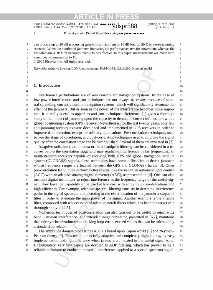
Fig. 1. Probability ratio concept, as referred to Neyman–Person and Capon works.

Reference [7] presents the results obtained in experiments on GPS P code, whil[6,10,11] show simulation results on coarse/acquisition (C/A) GPS code. But thedrawback of ADP filtering, as shown in [7,11] is the incapability to resist to scenhaving more than two simultaneous interferences.

Indeed, the ADP filter is really transparent to white Gaussian noise and to spspectrum navigation signals, by the same way allowing no deterioration of those sFor example, when 3 or 4 different jammers are present in the spectrum, the resultinability density function (PDF) tends to a Gaussian characteristic. Consequently, a temADP filter becomes unable to differ multiple interference from Gaussian noise. Bemost of interference is concentrated around a specific frequency range, the digitnal processing in the frequency domain will be more efficient. Multiple interferencebe easier to detect because its spectrum is completely different from the white Ganoise spectrum. Thus, after briefly reminding the principles of the ADP theory, thiper presents the differences between the spectral and the temporal ADP theories. Twhole structure of the ADP in the frequency domain (FADP) filter and the way it cainserted in a standard GPS receiver will be presented in detail. The last part of this paimed to expose the performances of the FADP filter and to compare the results withobtained using a temporal ADP filter.

2. Theoretical basis of the FADP filter

The ADP technique is based upon Capon work [8] and statistical theory of NeyPearson [9]. The main objective is to evaluate a probability ratioΛ(x), as function of thesamples of signalz(t), as statistically demonstrated in [12]. The presence or the absof the signal is determined by comparing this ratio to a decision thresholdµN (see Fig. 1).

This method is optimum insofar as the error probability (the probability to detect anal whereas there is no signal or not to detect a signal whereas there is one) is minFirst, the ADP filter theory will be elaborated. For more details, the reader could re[11,13,14]. Then, mathematical developments will be performed for the spectral reptation version of the ADP.

2.1. Elaboration of the ADP theory

The basis of this section can be found in [11], where some further elaborationsbeen considered. The same notation for the GPS signal application will be used in

UN



1 1

2 2

3 3

4 4

5 5

6 6

7 7

8 8

9 9

10 10

11 11

12 12

13 13

14 14

15 15

16 16

17 17

18 18

19 19

20 20

21 21

22 22

23 23

24 24

25 25

26 26

27 27

28 28

29 29

30 30

31 31

32 32

33 33

34 34

35 35

36 36

37 37

38 38

39 39

40 40

41 41

42 42

43 43

44 44

45 45

de be-

is to

Ac-ing:

rts

]),3) hassion of

applyec-dge of

CO

RR

EC

TE

D P

RO

OF

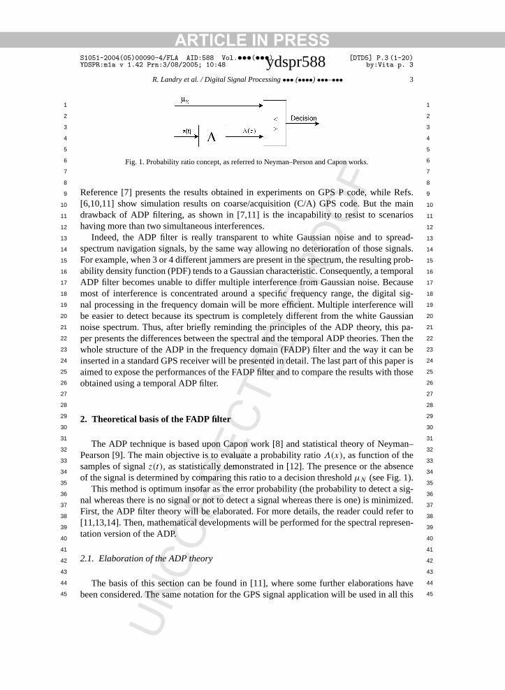
Fig. 2. Optimized theoretical receiver in rectangular coordinates.

paper. The signal captured by the GPS receiver can be written as following:

z(t) = r(t, θ) + w(t), (1)

r(t, θ) = s(t)cos(ωt + θ), (2)

where r(t) is the modulated information,s(t) is the useful data, andw(t) is a whiteGaussian noise including potential interference. The detection problem is to decitweenz(t) = r(t, θ) + w(t) andz(t) = w(t), when the signal is absent.

After extraction of the base band quadrature components, the detection problemdecide betweenxi = si cosθ + nxi ; yi = si sinθ + nyi andxi = nxi ; yi = nyi .

Let

fnn(x, y) =N∑

i=1

fnn(xi, yi)

be the input PDF ofz(t). It can be shown that this function is equal to the noise PDF.cording to [13], the optimal probability ratio evocated in Fig. 1 can be written as follow

Λ(wx,wy) − 1=[

1

N

N∑i=1

si∂fnn(xi, yi)/∂xi

fnn(xi, yi)

]2

+[

1

N

N∑i=1

si∂fnn(xi, yi)/∂yi

fnn(xi, yi)

]2

,

(3)

for a N -sampled complex signal, wherex andy represent the real and imaginary paof the signalz(t), wx andwy are the real and imaginary parts of the noisew(t) and sirepresents the samples of the signals(t). This formula, represented in Fig. 2 (see [13can be easily used in a conventional receiver to achieve its optimum form. Equation (been obtained by making use of the small-signal assumption and by using an expanfnn in a Taylor series around the values of the received data(xi, yi).

The drawback of the representation (3), while optimum, is that it is necessary toa non-linear function upon the two channelsI andQ (in phase and in quadrature, resptively), which doubles the required resources. Moreover, we need a perfect knowle

UN



1 1

2 2

3 3

4 4

5 5

6 6

7 7

8 8

9 9

10 10

11 11

12 12

13 13

14 14

15 15

16 16

17 17

18 18

19 19

20 20

21 21

22 22

23 23

24 24

25 25

26 26

27 27

28 28

29 29

30 30

31 31

32 32

33 33

34 34

35 35

36 36

37 37

38 38

39 39

40 40

41 41

42 42

43 43

44 44

45 45

. Ac-arrier

e,and its

thebtained

y

whered as in

.

CO

RR

EC

TE

D P

RO

OF

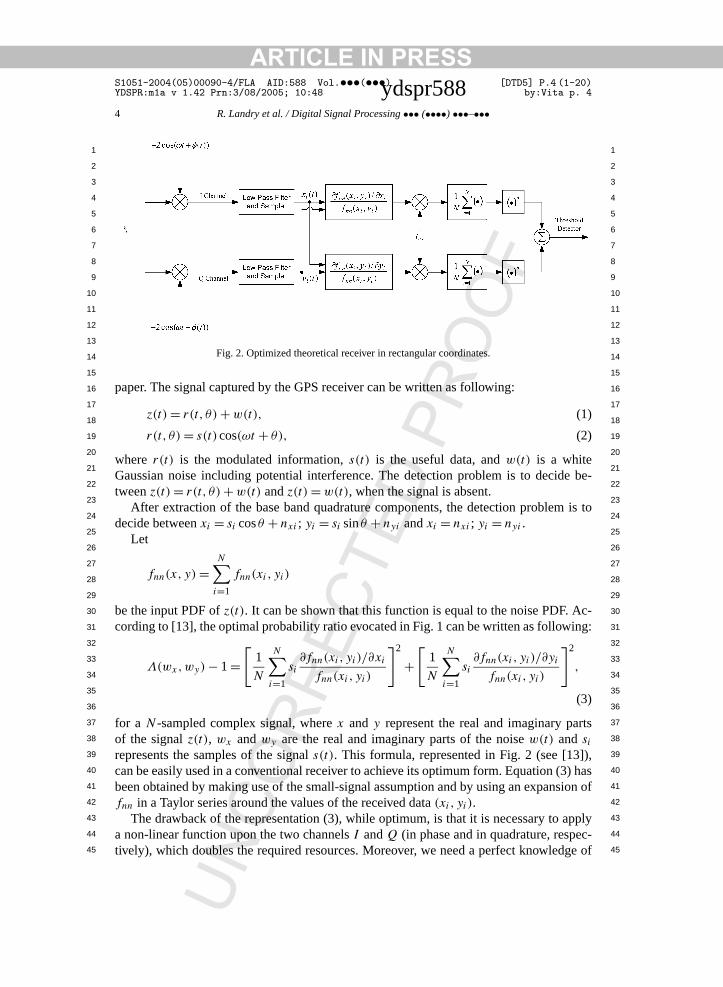
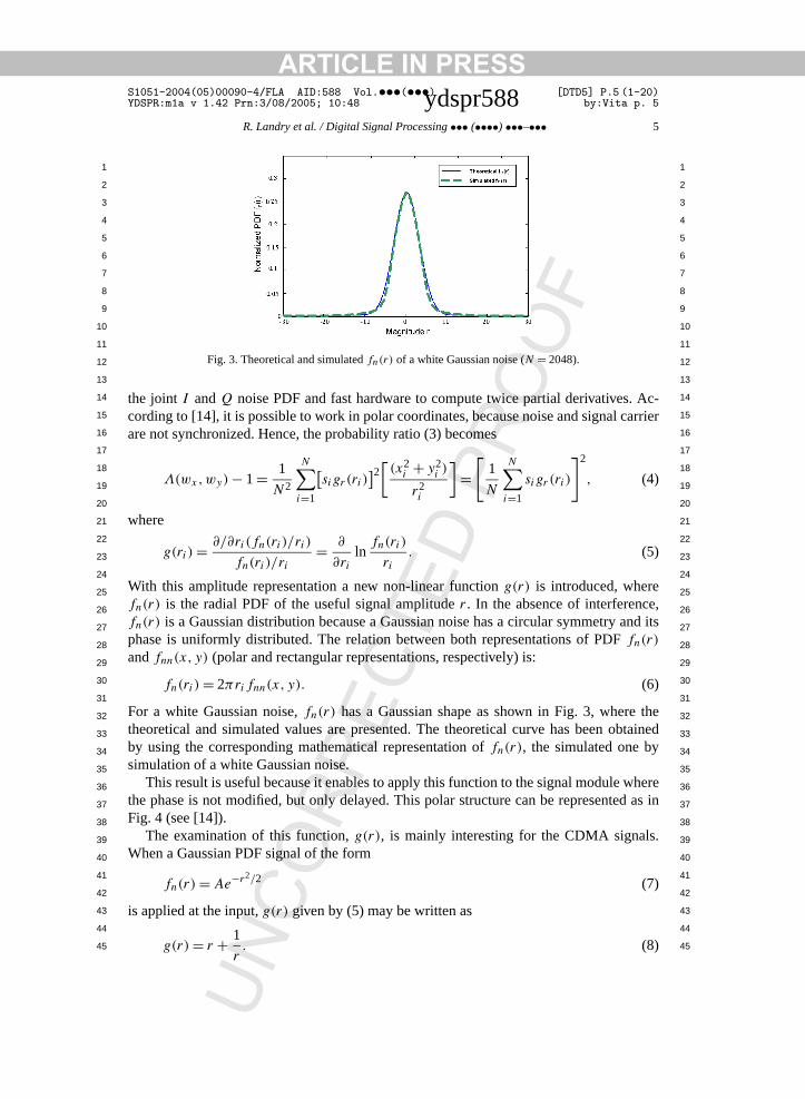
Fig. 3. Theoretical and simulatedfn(r) of a white Gaussian noise (N = 2048).

the joint I andQ noise PDF and fast hardware to compute twice partial derivativescording to [14], it is possible to work in polar coordinates, because noise and signal care not synchronized. Hence, the probability ratio (3) becomes

Λ(wx,wy) − 1= 1

N2

N∑i=1

[sigr(ri)

]2[(x2

i + y2i )

r2i

]=

[1

N

N∑i=1

sigr (ri)

]2

, (4)

where

g(ri) = ∂/∂ri(fn(ri)/ri)

fn(ri)/ri= ∂

∂riln

fn(ri)

ri. (5)

With this amplitude representation a new non-linear functiong(r) is introduced, wherefn(r) is the radial PDF of the useful signal amplituder . In the absence of interferencfn(r) is a Gaussian distribution because a Gaussian noise has a circular symmetryphase is uniformly distributed. The relation between both representations of PDFfn(r)

andfnn(x, y) (polar and rectangular representations, respectively) is:

fn(ri) = 2πrifnn(x, y). (6)

For a white Gaussian noise,fn(r) has a Gaussian shape as shown in Fig. 3, wheretheoretical and simulated values are presented. The theoretical curve has been oby using the corresponding mathematical representation offn(r), the simulated one bsimulation of a white Gaussian noise.

This result is useful because it enables to apply this function to the signal modulethe phase is not modified, but only delayed. This polar structure can be representeFig. 4 (see [14]).

The examination of this function,g(r), is mainly interesting for the CDMA signalsWhen a Gaussian PDF signal of the form

fn(r) = Ae−r2/2 (7)

is applied at the input,g(r) given by (5) may be written as

g(r) = r + 1. (8)

UNr



1 1

2 2

3 3

4 4

5 5

6 6

7 7

8 8

9 9

10 10

11 11

12 12

13 13

14 14

15 15

16 16

17 17

18 18

19 19

20 20

21 21

22 22

23 23

24 24

25 25

26 26

27 27

28 28

29 29

30 30

31 31

32 32

33 33

34 34

35 35

36 36

37 37

38 38

39 39

40 40

41 41

42 42

43 43

44 44

45 45

letally, therors.

ple

oflues,ositive

itive

pon

(seef being
C
OR

RE

CTE

D P

RO

OF

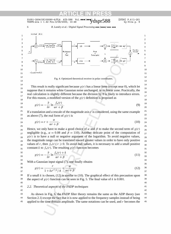
Fig. 4. Optimized theoretical receiver in polar coordinates.

This result is really significant becauseg(r) has a linear form (except near 0), whichsuppose that it remains white Gaussian noise unchanged, in its linear zone. Practicreal calculation is slightly different because the division by 0 is likely to introduce erFor this reason, a modified version of theg(r) definition is proposed as

g(r) = − ∂

∂rln

fn(r)

αr + β. (9)

If a translation and a rescale of the magnitude axisr is considered, using the same examas above (7), the real form ofg(r) is

g(r) = r + α

αr + β. (10)

Hence, we only have to make a good choice ofα andβ to make the second term ofg(r)

negligible (e.g.,α = 0.08 andβ = 110). Another delicate point of the computationg(r) is to have a null or negative argument of the logarithm. To avoid negative vathe magnitude range can be translated toward greater values in order to have only pvalues ofr , thenfn(r)/r � 0. To avoid null values, it is necessary to add a small posconstantk to fn(r). The resultingg(r) function becomes

g(r) = − ∂

∂rln

fn(r) + k

αr + β. (11)

With a Gaussian input signal (7), one finally obtains

g(r) = r

1+ ker2/2/A+ α

αr + β. (12)

If a smallk is chosen, (12) is similar to (10). The graphical effect of this precaution uthe aspect ofg(r) function can be seen in Fig. 5. The final value ofk is 0.001.

2.2. Theoretical aspects of the FADP techniques

As shown in Fig. 6, the FADP filter theory remains the same as the ADP theorySection 2.1) except the fact that it is now applied to the frequency samples instead oapplied to the time domain amplitude. The same notations can be used, andr becomes the

UN



1 1

2 2

3 3

4 4

5 5

6 6

7 7

8 8

9 9

10 10

11 11

12 12

13 13

14 14

15 15

16 16

17 17

18 18

19 19

20 20

21 21

22 22

23 23

24 24

25 25

26 26

27 27

28 28

29 29

30 30

31 31

32 32

33 33

34 34

35 35

36 36

37 37

38 38

39 39

40 40

41 41

42 42

43 43

44 44

45 45

use

a reallo polaring a

mean0 afterider

CO

RR

EC

TE

D P

RO

OF

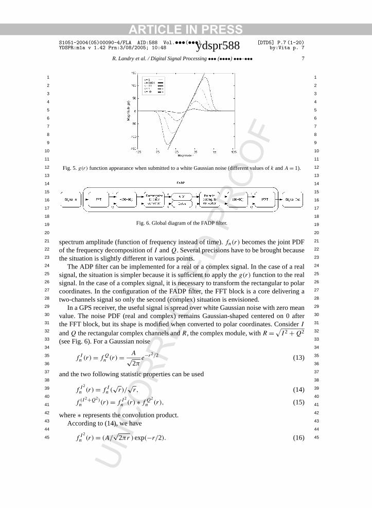
Fig. 5.g(r) function appearance when submitted to a white Gaussian noise (different values ofk andA = 1).

Fig. 6. Global diagram of the FADP filter.

spectrum amplitude (function of frequency instead of time).fn(r) becomes the joint PDFof the frequency decomposition ofI andQ. Several precisions have to be brought becathe situation is slightly different in various points.

The ADP filter can be implemented for a real or a complex signal. In the case ofsignal, the situation is simpler because it is sufficient to apply theg(r) function to the reasignal. In the case of a complex signal, it is necessary to transform the rectangular tcoordinates. In the configuration of the FADP filter, the FFT block is a core delivertwo-channels signal so only the second (complex) situation is envisioned.

In a GPS receiver, the useful signal is spread over white Gaussian noise with zerovalue. The noise PDF (real and complex) remains Gaussian-shaped centered onthe FFT block, but its shape is modified when converted to polar coordinates. ConsI

andQ the rectangular complex channels andR, the complex module, withR = √I2 + Q2

(see Fig. 6). For a Gaussian noise

f In (r) = f Q

n (r) = A√2π

e−r2/2 (13)

and the two following statistic properties can be used

f I2

n (r) = f In (

√r)/

√r, (14)

f (I2+Q2)n (r) = f I2

n (r) ∗ f Q2

n (r), (15)

where∗ represents the convolution product.According to (14), we have

f I2

n (r) = (A/√

2πr )exp(−r/2). (16)

UN



1 1

2 2

3 3

4 4

5 5

6 6

7 7

8 8

9 9

10 10

11 11

12 12

13 13

14 14

15 15

16 16

17 17

18 18

19 19

20 20

21 21

22 22

23 23

24 24

25 25

26 26

27 27

28 28

29 29

30 30

31 31

32 32

33 33

34 34

35 35

36 36

37 37

38 38

39 39

40 40

41 41

42 42

43 43

44 44

45 45

d at thelineare

rans-

,
CO
RR

EC

TE

D P

RO

OF

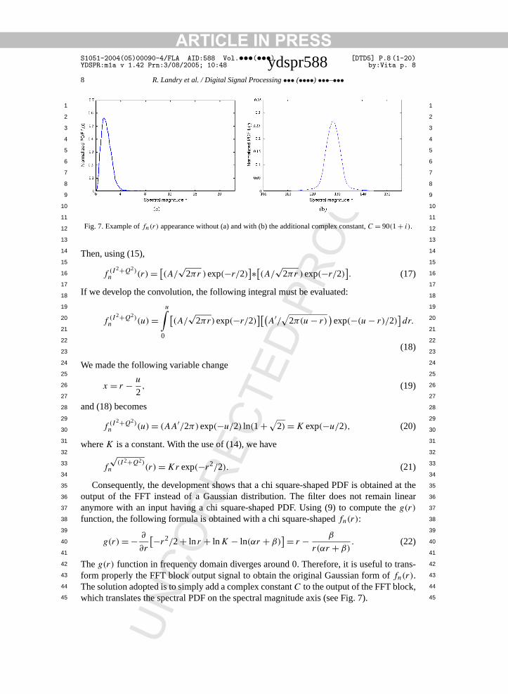
Fig. 7. Example offn(r) appearance without (a) and with (b) the additional complex constant,C = 90(1+ i).

Then, using (15),

f (I2+Q2)n (r) = [

(A/√

2πr )exp(−r/2)]∗[

(A/√

2πr )exp(−r/2)]. (17)

If we develop the convolution, the following integral must be evaluated:

f (I2+Q2)n (u) =

u∫0

[(A/

√2πr)exp(−r/2)

][(A′/

√2π(u − r)

)exp(−(u − r)/2)

]dr.

(18)

We made the following variable change

x = r − u

2, (19)

and (18) becomes

f (I2+Q2)n (u) = (AA′/2π)exp(−u/2) ln(1+ √

2) = K exp(−u/2), (20)

whereK is a constant. With the use of (14), we have

f

√(I2+Q2)

n (r) = Kr exp(−r2/2). (21)

Consequently, the development shows that a chi square-shaped PDF is obtaineoutput of the FFT instead of a Gaussian distribution. The filter does not remainanymore with an input having a chi square-shaped PDF. Using (9) to compute thg(r)

function, the following formula is obtained with a chi square-shapedfn(r):

g(r) = − ∂

∂r

[−r2/2+ ln r + lnK − ln(αr + β)] = r − β

r(αr + β). (22)

Theg(r) function in frequency domain diverges around 0. Therefore, it is useful to tform properly the FFT block output signal to obtain the original Gaussian form offn(r).The solution adopted is to simply add a complex constantC to the output of the FFT blockwhich translates the spectral PDF on the spectral magnitude axis (see Fig. 7).

UN



1 1

2 2

3 3

4 4

5 5

6 6

7 7

8 8

9 9

10 10

11 11

12 12

13 13

14 14

15 15

16 16

17 17

18 18

19 19

20 20

21 21

22 22

23 23

24 24

25 25

26 26

27 27

28 28

29 29

30 30

31 31

32 32

33 33

34 34

35 35

36 36

37 37

38 38

39 39

40 40

41 41

42 42

43 43

44 44

45 45

odulee-

iently

upondifferof the

ocess-

they aree in-to the

he fil-eory

spec-andards,redcon-etweenorder

.in ad-
C
OR

RE

CTE

D P

RO

OF

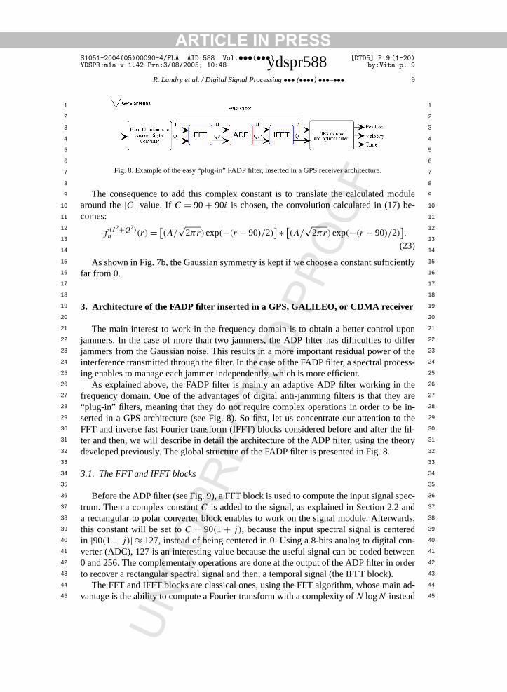
Fig. 8. Example of the easy “plug-in” FADP filter, inserted in a GPS receiver architecture.

The consequence to add this complex constant is to translate the calculated maround the|C| value. If C = 90+ 90i is chosen, the convolution calculated in (17) bcomes:

f (I2+Q2)n (r) = [

(A/√

2πr)exp(−(r − 90)/2)] ∗ [

(A/√

2πr)exp(−(r − 90)/2)].

(23)

As shown in Fig. 7b, the Gaussian symmetry is kept if we choose a constant sufficfar from 0.

3. Architecture of the FADP filter inserted in a GPS, GALILEO, or CDMA receiver

The main interest to work in the frequency domain is to obtain a better controljammers. In the case of more than two jammers, the ADP filter has difficulties tojammers from the Gaussian noise. This results in a more important residual powerinterference transmitted through the filter. In the case of the FADP filter, a spectral pring enables to manage each jammer independently, which is more efficient.

As explained above, the FADP filter is mainly an adaptive ADP filter working infrequency domain. One of the advantages of digital anti-jamming filters is that the“plug-in” filters, meaning that they do not require complex operations in order to bserted in a GPS architecture (see Fig. 8). So first, let us concentrate our attentionFFT and inverse fast Fourier transform (IFFT) blocks considered before and after tter and then, we will describe in detail the architecture of the ADP filter, using the thdeveloped previously. The global structure of the FADP filter is presented in Fig. 8.

3.1. The FFT and IFFT blocks

Before the ADP filter (see Fig. 9), a FFT block is used to compute the input signaltrum. Then a complex constantC is added to the signal, as explained in Section 2.2a rectangular to polar converter block enables to work on the signal module. Afterwthis constant will be set toC = 90(1 + j), because the input spectral signal is centein |90(1 + j)| ≈ 127, instead of being centered in 0. Using a 8-bits analog to digitalverter (ADC), 127 is an interesting value because the useful signal can be coded b0 and 256. The complementary operations are done at the output of the ADP filter into recover a rectangular spectral signal and then, a temporal signal (the IFFT block)

The FFT and IFFT blocks are classical ones, using the FFT algorithm, whose mavantage is the ability to compute a Fourier transform with a complexity ofN logN instead

UN



1 1

2 2

3 3

4 4

5 5

6 6

7 7

8 8

9 9

10 10

11 11

12 12

13 13

14 14

15 15

16 16

17 17

18 18

19 19

20 20

21 21

22 22

23 23

24 24

25 25

26 26

27 27

28 28

29 29

30 30

31 31

32 32

33 33

34 34

35 35

36 36

37 37

38 38

39 39

40 40

41 41

42 42

43 43

44 44

45 45

-hosen

filtertails

tationreimeains aing
C
OR

RE

CTE

D P

RO

OF

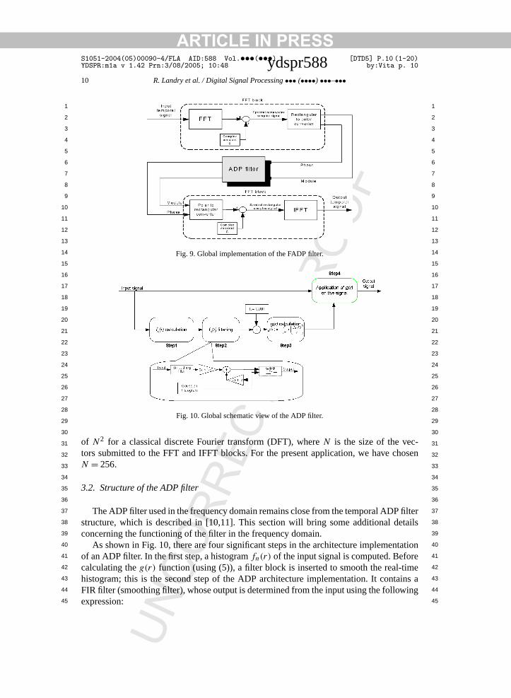
Fig. 9. Global implementation of the FADP filter.

Fig. 10. Global schematic view of the ADP filter.

of N2 for a classical discrete Fourier transform (DFT), whereN is the size of the vectors submitted to the FFT and IFFT blocks. For the present application, we have cN = 256.

3.2. Structure of the ADP filter

The ADP filter used in the frequency domain remains close from the temporal ADPstructure, which is described in [10,11]. This section will bring some additional deconcerning the functioning of the filter in the frequency domain.

As shown in Fig. 10, there are four significant steps in the architecture implemenof an ADP filter. In the first step, a histogramfn(r) of the input signal is computed. Befocalculating theg(r) function (using (5)), a filter block is inserted to smooth the real-thistogram; this is the second step of the ADP architecture implementation. It contFIR filter (smoothing filter), whose output is determined from the input using the followexpression:

UN



1 1

2 2

3 3

4 4

5 5

6 6

7 7

8 8

9 9

10 10

11 11

12 12

13 13

14 14

15 15

16 16

17 17

18 18

19 19

20 20

21 21

22 22

23 23

24 24

25 25

26 26

27 27

28 28

29 29

30 30

31 31

32 32

33 33

34 34

35 35

36 36

37 37

38 38

39 39

40 40

41 41

42 42

43 43

44 44

45 45

input

tly,in theless

teat the

of(e.g.,eP

l ADPutputd

f 0,

stingGC),r for

Then,

reatedquencemdom se-2a willuency

CO

RR

EC

TE

D P

RO

OF

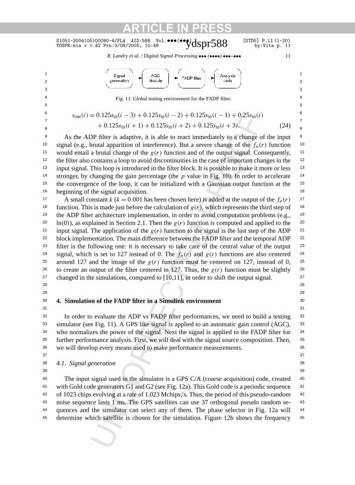
Fig. 11. Global testing environment for the FADP filter.

sout(i) = 0.125sin(i − 3) + 0.125sin(i − 2) + 0.125sin(i − 1) + 0.25sin(i)

+ 0.125sin(i + 1) + 0.125sin(i + 2) + 0.125sin(i + 3). (24)

As the ADP filter is adaptive, it is able to react immediately to a change of thesignal (e.g., brutal apparition of interference). But a severe change of thefn(r) functionwould entail a brutal change of theg(r) function and of the output signal. Consequenthe filter also contains a loop to avoid discontinuities in the case of important changesinput signal. This loop is introduced in the filter block. It is possible to make it more orstronger, by changing the gain percentage (thep value in Fig. 10). In order to accelerathe convergence of the loop, it can be initialized with a Gaussian output functionbeginning of the signal acquisition.

A small constantk (k = 0.001 has been chosen here) is added at the output of thefn(r)

function. This is made just before the calculation ofg(r), which represents the third stepthe ADP filter architecture implementation, in order to avoid computation problemsln(0)), as explained in Section 2.1. Then theg(r) function is computed and applied to thinput signal. The application of theg(r) function to the signal is the last step of the ADblock implementation. The main difference between the FADP filter and the temporafilter is the following one: it is necessary to take care of the central value of the osignal, which is set to 127 instead of 0. Thefn(r) andg(r) functions are also centerearound 127 and the image of theg(r) function must be centered on 127, instead oto create an output of the filter centered in 127. Thus, theg(r) function must be slightlychanged in the simulations, compared to [10,11], in order to shift the output signal.

4. Simulation of the FADP filter in a Simulink environment

In order to evaluate the ADP vs FADP filter performances, we need to build a tesimulator (see Fig. 11). A GPS like signal is applied to an automatic gain control (Awho normalizes the power of the signal. Next the signal is applied to the FADP filtefurther performance analysis. First, we will deal with the signal source composition.we will develop every means used to make performance measurements.

4.1. Signal generation

The input signal used in the simulator is a GPS C/A (coarse acquisition) code, cwith Gold code generators G1 and G2 (see Fig. 12a). This Gold code is a periodic seof 1023 chips evolving at a rate of 1.023 Mchips/s. Thus, the period of this pseudo-randonoise sequence lasts 1 ms. The GPS satellites can use 37 orthogonal pseudo ranquences and the simulator can select any of them. The phase selector in Fig. 1determine which satellite is chosen for the simulation. Figure 12b shows the freq

UN



1 1

2 2

3 3

4 4

5 5

6 6

7 7

8 8

9 9

10 10

11 11

12 12

13 13

14 14

15 15

16 16

17 17

18 18

19 19

20 20

21 21

22 22

23 23

24 24

25 25

26 26

27 27

28 28

29 29

30 30

31 31

32 32

33 33

34 34

35 35

36 36

37 37

38 38

39 39

40 40

41 41

42 42

43 43

44 44

45 45

rate of

er ofwith

nd theentire

f jam-

jam-ctrum.

DARnted in

tionuencypectrally.

CO

RR

EC

TE

D P

RO

OF

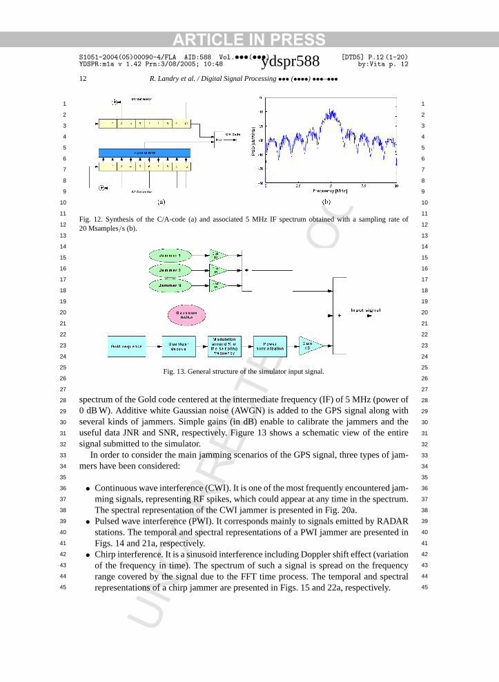
Fig. 12. Synthesis of the C/A-code (a) and associated 5 MHz IF spectrum obtained with a sampling20 Msamples/s (b).

Fig. 13. General structure of the simulator input signal.

spectrum of the Gold code centered at the intermediate frequency (IF) of 5 MHz (pow0 dB W). Additive white Gaussian noise (AWGN) is added to the GPS signal alongseveral kinds of jammers. Simple gains (in dB) enable to calibrate the jammers auseful data JNR and SNR, respectively. Figure 13 shows a schematic view of thesignal submitted to the simulator.

In order to consider the main jamming scenarios of the GPS signal, three types omers have been considered:

• Continuous wave interference (CWI). It is one of the most frequently encounteredming signals, representing RF spikes, which could appear at any time in the speThe spectral representation of the CWI jammer is presented in Fig. 20a.

• Pulsed wave interference (PWI). It corresponds mainly to signals emitted by RAstations. The temporal and spectral representations of a PWI jammer are preseFigs. 14 and 21a, respectively.

• Chirp interference. It is a sinusoid interference including Doppler shift effect (variaof the frequency in time). The spectrum of such a signal is spread on the freqrange covered by the signal due to the FFT time process. The temporal and srepresentations of a chirp jammer are presented in Figs. 15 and 22a, respective

UN



1 1

2 2

3 3

4 4

5 5

6 6

7 7

8 8

9 9

10 10

11 11

12 12

13 13

14 14

15 15

16 16

17 17

18 18

19 19

20 20

21 21

22 22

23 23

24 24

25 25

26 26

27 27

28 28

29 29

30 30

31 31

32 32

33 33

34 34

35 35

36 36

37 37

38 38

39 39

40 40

41 41

42 42

43 43

44 44

45 45

.

ify thecorre-

ence ofhese

rloss ison why

of itsthe linkcreas-

mentsio willn be
C
OR

RE

CTE

D P

RO

OF

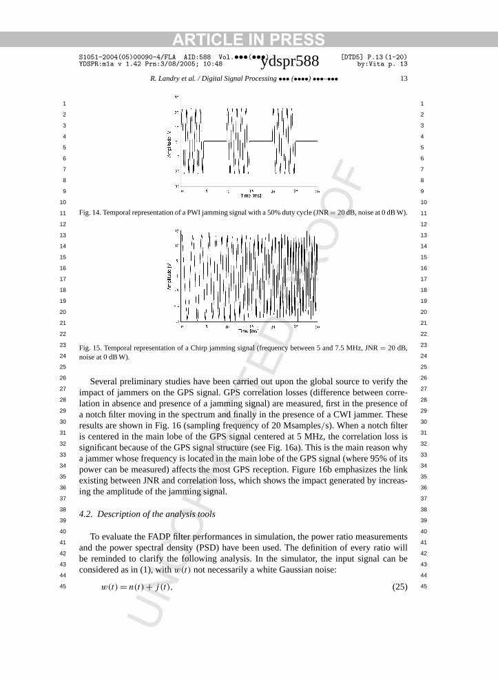
Fig. 14. Temporal representation of a PWI jamming signal with a 50% duty cycle (JNR= 20 dB, noise at 0 dB W)

Fig. 15. Temporal representation of a Chirp jamming signal (frequency between 5 and 7.5 MHz, JNR= 20 dB,noise at 0 dB W).

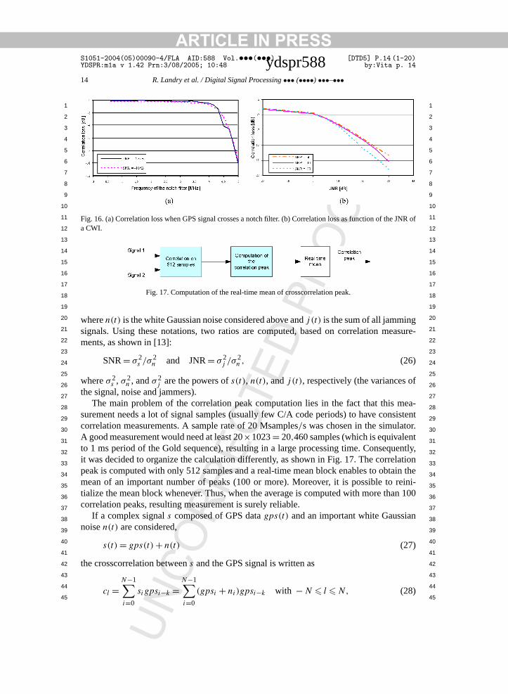
Several preliminary studies have been carried out upon the global source to verimpact of jammers on the GPS signal. GPS correlation losses (difference betweenlation in absence and presence of a jamming signal) are measured, first in the presa notch filter moving in the spectrum and finally in the presence of a CWI jammer. Tresults are shown in Fig. 16 (sampling frequency of 20 Msamples/s). When a notch filteis centered in the main lobe of the GPS signal centered at 5 MHz, the correlationsignificant because of the GPS signal structure (see Fig. 16a). This is the main reasa jammer whose frequency is located in the main lobe of the GPS signal (where 95%power can be measured) affects the most GPS reception. Figure 16b emphasizesexisting between JNR and correlation loss, which shows the impact generated by ining the amplitude of the jamming signal.

4.2. Description of the analysis tools

To evaluate the FADP filter performances in simulation, the power ratio measureand the power spectral density (PSD) have been used. The definition of every ratbe reminded to clarify the following analysis. In the simulator, the input signal caconsidered as in (1), withw(t) not necessarily a white Gaussian noise:

w(t) = n(t) + j (t), (25)

UN



1 1

2 2

3 3

4 4

5 5

6 6

7 7

8 8

9 9

10 10

11 11

12 12

13 13

14 14

15 15

16 16

17 17

18 18

19 19

20 20

21 21

22 22

23 23

24 24

25 25

26 26

27 27

28 28

29 29

30 30

31 31

32 32

33 33

34 34

35 35

36 36

37 37

38 38

39 39

40 40

41 41

42 42

43 43

44 44

45 45

JNR of

easure-

of

mea-sistentr.

ntuently,lationain thereini-an 100

n

CO

RR

EC

TE

D P

RO

OF

Fig. 16. (a) Correlation loss when GPS signal crosses a notch filter. (b) Correlation loss as function of thea CWI.

Fig. 17. Computation of the real-time mean of crosscorrelation peak.

wheren(t) is the white Gaussian noise considered above andj (t) is the sum of all jammingsignals. Using these notations, two ratios are computed, based on correlation mments, as shown in [13]:

SNR= σ 2s /σ 2

n and JNR= σ 2j /σ 2

n , (26)

whereσ 2s , σ 2

n , andσ 2j are the powers ofs(t), n(t), andj (t), respectively (the variances

the signal, noise and jammers).The main problem of the correlation peak computation lies in the fact that this

surement needs a lot of signal samples (usually few C/A code periods) to have concorrelation measurements. A sample rate of 20 Msamples/s was chosen in the simulatoA good measurement would need at least 20×1023= 20,460 samples (which is equivaleto 1 ms period of the Gold sequence), resulting in a large processing time. Conseqit was decided to organize the calculation differently, as shown in Fig. 17. The correpeak is computed with only 512 samples and a real-time mean block enables to obtmean of an important number of peaks (100 or more). Moreover, it is possible totialize the mean block whenever. Thus, when the average is computed with more thcorrelation peaks, resulting measurement is surely reliable.

If a complex signals composed of GPS datagps(t) and an important white Gaussianoisen(t) are considered,

s(t) = gps(t) + n(t) (27)

the crosscorrelation betweens and the GPS signal is written as

cl =N−1∑

sigpsi−k =N−1∑

(gpsi + ni)gpsi−k with − N � l � N, (28)

UNi=0 i=0



1 1

2 2

3 3

4 4

5 5

6 6

7 7

8 8

9 9

10 10

11 11

12 12

13 13

14 14

15 15

16 16

17 17

18 18

19 19

20 20

21 21

22 22

23 23

24 24

25 25

26 26

27 27

28 28

29 29

30 30

31 31

32 32

33 33

34 34

35 35

36 36

37 37

38 38

39 39

40 40

41 41

42 42

43 43

44 44

45 45

e GPSwe con-aloise and

to the

scorre-noise

he JNRfiltervaluessame

d JNR.ks, as

lity ofloss

ion loss

cy, as

alcom-

CO

RR

EC

TE

D P

RO

OF

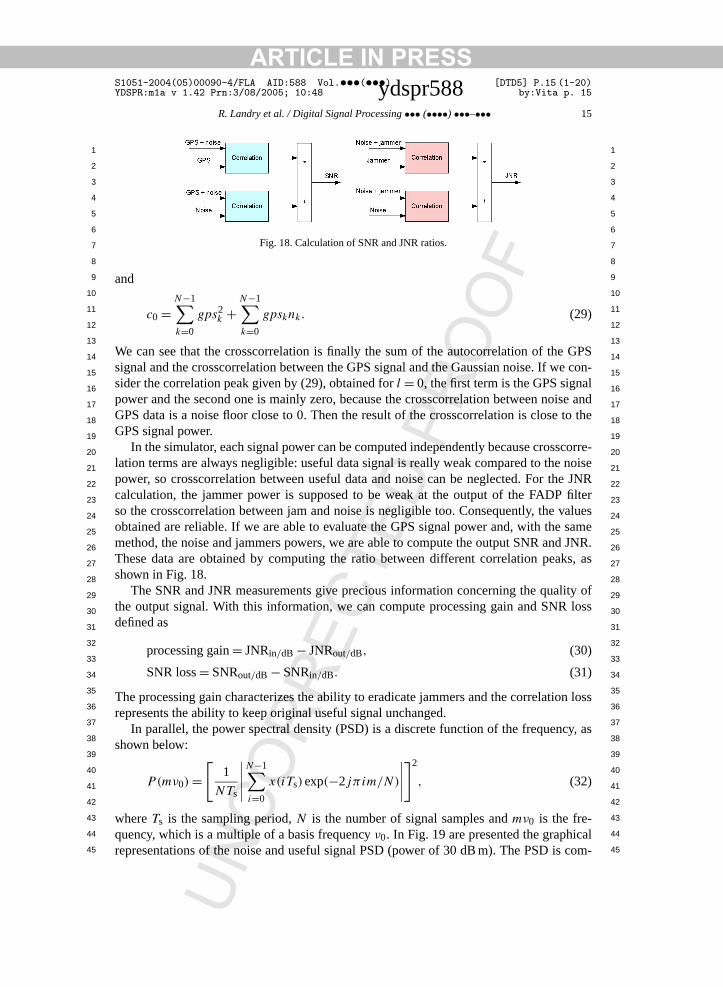
Fig. 18. Calculation of SNR and JNR ratios.

and

c0 =N−1∑k=0

gps2k +

N−1∑k=0

gpsknk. (29)

We can see that the crosscorrelation is finally the sum of the autocorrelation of thsignal and the crosscorrelation between the GPS signal and the Gaussian noise. Ifsider the correlation peak given by (29), obtained forl = 0, the first term is the GPS signpower and the second one is mainly zero, because the crosscorrelation between nGPS data is a noise floor close to 0. Then the result of the crosscorrelation is closeGPS signal power.

In the simulator, each signal power can be computed independently because croslation terms are always negligible: useful data signal is really weak compared to thepower, so crosscorrelation between useful data and noise can be neglected. For tcalculation, the jammer power is supposed to be weak at the output of the FADPso the crosscorrelation between jam and noise is negligible too. Consequently, theobtained are reliable. If we are able to evaluate the GPS signal power and, with themethod, the noise and jammers powers, we are able to compute the output SNR anThese data are obtained by computing the ratio between different correlation peashown in Fig. 18.

The SNR and JNR measurements give precious information concerning the quathe output signal. With this information, we can compute processing gain and SNRdefined as

processing gain= JNRin/dB − JNRout/dB, (30)

SNR loss= SNRout/dB − SNRin/dB. (31)

The processing gain characterizes the ability to eradicate jammers and the correlatrepresents the ability to keep original useful signal unchanged.

In parallel, the power spectral density (PSD) is a discrete function of the frequenshown below:

P(mν0) =[

1

NTs

∣∣∣∣∣N−1∑i=0

x(iTs)exp(−2jπim/N)

∣∣∣∣∣]2

, (32)

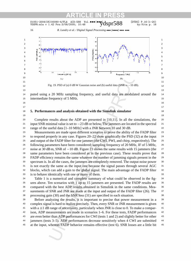
whereTs is the sampling period,N is the number of signal samples andmν0 is the fre-quency, which is a multiple of a basis frequencyν0. In Fig. 19 are presented the graphicrepresentations of the noise and useful signal PSD (power of 30 dB m). The PSD is

UN



1 1

2 2

3 3

4 4

5 5

6 6

7 7

8 8

9 9

10 10

11 11

12 12

13 13

14 14

15 15

16 16

17 17

18 18

19 19

20 20

21 21

22 22

23 23

24 24

25 25

26 26

27 27

28 28

29 29

30 30

31 31

32 32

33 33

34 34

35 35

36 36

37 37

38 38

39 39

40 40

41 41

42 42

43 43

44 44

45 45

nd the

s, thetral

filtere inputThe

MHz,(therove thatt in thepower

ral AGCfilter

e fig-ults areMea-). The

t in agivenpar-

mancesr othermitted

ttle bit

CO

RR

EC

TE

D P

RO

OF

Fig. 19. PSD of (a) 0 dB W Gaussian noise and (b) useful data (SNR= −10 dB).

puted using a 20 MHz sampling frequency, and useful data are modulated arouintermediate frequency of 5 MHz.

5. Performances and analysis obtained with the Simulink simulator

Complete results about the ADP are presented in [10,11]. In all the simulationinput SNR minimal value is set to−23 dB or below. The jammers are located in the specrange of the useful data [1–10 MHz] with a JNR between 10 and 30 dB.

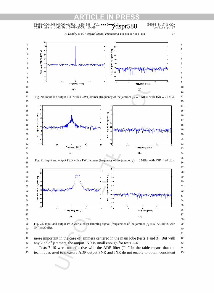
Measurements are made upon different scenarios to prove the ability of the FADPto respond properly in any case. Figures 20–22 show graphically the PSD (32) at thand output of the FADP filter for one jammer (the CWI, PWI, and chirp, respectively).following parameters have been considered: sampling frequency of 20 MHz, IF of 5noise at 30 dB m, SNR of−10 dB. Figure 23 shows the same results with 15 jammerssame parameters have been considered as in the previous case). These results pFADP efficiency remains the same whatever the number of jamming signals presenspectrum is. In all the cases, the jammers are completely removed. The output noiseis not exactly the same as the input one because the signal passes through seveblocks, which can add a gain to the global signal. The main advantage of the FADPis to behave identically with one or many of them.

Table 1 is a numerical and complete summary of what could be observed in thures above. Ten scenarios with 1 up to 15 jammers are presented. The FADP rescompared with the best ADP results obtained in Simulink in the same conditions.surements of SNR and JNR are made at the input and output of the FADP filter (26processing gain (30) and the SNR loss (31) are specified in each situation.

Before analyzing the results, it is important to precise that power measuremencomplex signal is hard to realize precisely. Then, every SNR or JNR measurement iswith a±1 dB range of uncertainty, particularly when JNR is close to 0. To make a comison, ADP measurements are made in scenarios 1–6. For these tests, FADP perforare even better than ADP performances for CWI (tests 1 and 2) and slightly better fojammers (tests 3–5). ADP performances decrease sensitively when 4 CWI are subat the input, whereas FADP behavior remains effective (test 6). SNR losses are a li

UN



1 1

2 2

3 3

4 4

5 5

6 6

7 7

8 8

9 9

10 10

11 11

12 12

13 13

14 14

15 15

16 16

17 17

18 18

19 19

20 20

21 21

22 22

23 23

24 24

25 25

26 26

27 27

28 28

29 29

30 30

31 31

32 32

33 33

34 34

35 35

36 36

37 37

38 38

39 39

40 40

41 41

42 42

43 43

44 44

45 45

ut with

esistent

CO

RR

EC

TE

D P

RO

OF

Fig. 20. Input and output PSD with a CWI jammer (frequency of the jammerfj = 5 MHz, with JNR= 20 dB).

Fig. 21. Input and output PSD with a PWI jammer (frequency of the jammerfj = 5 MHz, with JNR= 20 dB).

Fig. 22. Input and output PSD with a chirp jamming signal (frequencies of the jammerfj = 5–7.5 MHz, withJNR= 20 dB).

more important in the case of jammers centered in the main lobe (tests 1 and 3). Bany kind of jammers, the output JNR is small enough for tests 1–6.

Tests 7–10 were not effective with the ADP filter (“−” in the table means that thtechniques used to measure ADP output SNR and JNR do not enable to obtain con

UN



1 1

2 2

3 3

4 4

5 5

6 6

7 7

8 8

9 9

10 10

11 11

12 12

13 13

14 14

15 15

16 16

17 17

18 18

19 19

20 20

21 21

22 22

23 23

24 24

25 25

26 26

27 27

28 28

29 29

30 30

31 31

32 32

33 33

34 34

35 35

36 36

37 37

38 38

39 39

40 40

41 41

42 42

43 43

44 44

45 45

morempor-l datanal isglobalsed ofg en-

ormal-wnedl-

elationated be-lets
C
OR

RE

CTE

D P

RO

OF

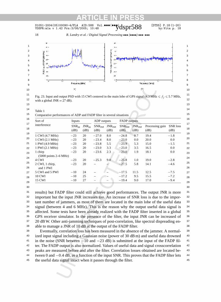
Fig. 23. Input and output PSD with 15 CWI centered in the main lobe of GPS signal (4.3 MHz� fj � 5.7 MHz,with a global JNR= 27 dB).

Table 1Comparative performances of ADP and FADP filter in several situations

Sort ofinterference

Inputs ADP outputs FADP outputs

SNRin(dB)

JNRin(dB)

SNRout(dB)

JNRout(dB)

SNRout(dB)

JNRout(dB)

Processing gain(dB)

SNR loss(dB)

1 CWI (4.7 MHz) −23 20 −27.0 8.0 −24.8 0.7 19.4 −1.81 CWI (2.1 MHz) −23 20 −23.4 8.0 −23.0 0.0 20.0 0.01 PWI (4.9 MHz) −23 20 −23.8 5.5 −23.9 5.3 15.0 −1.51 PWI (2.1 MHz) −23 20 −23.0 3.3 −23.0 3.5 16.5 0.01 chirp

(5000 points 2–6 MHz)−23 20 −23.6 2.3 −23.0 1.9 18.1 0.0

4 CWI −23 20 −25.3 9.0 −25.8 1.0 19.0 −2.82 CWI, 1 chirp,

and 1 PWI−23 20 – – −27.5 5.8 14.1 −4.6

5 CWI and 5 PWI −10 24 – – −17.5 11.5 12.5 −7.510 CWI −10 25 – – −17.2 9.5 15.5 −7.215 CWI −10 27 – – −19.4 9.0 17.0 −9.4

results) but FADP filter could still achieve good performances. The output JNR isimportant but the input JNR increases too. An increase of SNR loss is due to the itant number of jammers, as most of them are located in the main lobe of the usefusignal (between 4 and 6 MHz). This is the reason why the output useful data sigaffected. Some tests have been already realized with the FADP filter inserted in aGPS receiver simulator. In the presence of the filter, the input JNR can be increa20 dB W. Other anti-jamming techniques of post-correlation, like spectral dispreadinable to manage a JNR of 10 dB at the output of the FADP filter.

Eventually, correlation loss has been measured in the absence of the jammer. A nized input signal including a Gaussian noise (power of 30 dB m) and useful data droin the noise (SNR between−10 and−23 dB) is submitted at the input of the FADP fiter. The FADP output is also normalized. Values of useful data and signal crosscorrpeaks are measured before and after the filter. Correlation losses obtained are loctween 0 and−0.4 dB, as a function of the input SNR. This proves that the FADP filterthe useful data signal intact when it passes through the filter.

UN



1 1

2 2

3 3

4 4

5 5

6 6

7 7

8 8

9 9

10 10

11 11

12 12

13 13

14 14

15 15

16 16

17 17

18 18

19 19

20 20

21 21

22 22

23 23

24 24

25 25

26 26

27 27

28 28

29 29

30 30

31 31

32 32

33 33

34 34

35 35

36 36

37 37

38 38

39 39

40 40

41 41

42 42

43 43

44 44

45 45

ms ist. In

l anti-lter;cksets.to workhe per-ce ofectralchirp,educedred in

PS/s ofelopedproof

order toP filter

d Nav-

d’Etudesulouse,

tions forystems,

unica-

sment ofpplica-

(1988)

eedings

Theory

port,

ana-

CO

RR

EC

TE

D P

RO

OF

6. Conclusions

One of the main concerns with the use of the GPS and other positioning systethe ability to operate in all conditions and to maintain integrity in hostile environmenthis paper, we have shown that the FADP filtering could open new horizons in digitajamming techniques. Digital processing in the FADP filter is pretty close to the ADP fino important changes being necessary except the addition of the FFT and IFFT bloThen, measurement techniques have been the object of great thinking to be ableas precise as possible in real conditions. In the presence of one or two jammers, tformances of the FADP filter are equivalent to those of the ADP filter. In the presenmore jammers, the FADP filter has shown to be more effective than the ADP one. Spprocessing enables to eradicate precisely all sorts of jammers, like PWI, CWI andwhose frequencies are located in the main lobe of a GPS Gold sequence. JNR is rfrom at least 12 up to 20 dB when passing through the filter. Correlation loss, measuabsence of jammers, is under 0.5 dB in any case.

Further investigations will be done with the FADP filter inserted in an entire GGALILEO receiver Simulink model, in order to study its impact on the performancethe receiver. The simulation that we have evocated here with Simulink has been devin order to be easily translated and implemented in a FPGA component. Real-timeof concept demonstrator has been designed to be inserted in real GPS receiver inmeasure real performance of such a filter. Moreover, the great advantage of the FADis its easy “plug-in” ability, enabling to insert it in any kind of CDMA receivers.

References

[1] A. Ndili, D.P. Enge, GPS receiver autonomous interference detection, in: IEEE Position, Location anigation Symposium—PLANS 98, Palm Spring, CA, 1998.

[2] R.J. Landry, Techniques de Robustesse aux Brouilleurs pour les Récepteurs GPS, in: Départementet de Recherches en Automatique DERA/CERT et du Laboratoire Electronique et Physique, ToFrance, 1997, pp. 58–115.

[3] R.J. Landry, A. Renard, Analysis of potential interference sources and assessment of present soluGPS/GNSS receivers, in: Fourth St. Petersburg International Conference on Integrated Navigation SSt. Petersburg, 1997.

[4] F. Amoroso, Adaptive A/D converter to suppress CW interference in DSPN spread-spectrum commtions, IEEE Trans. Commun. COM-31 (10) (1983) 1117–1123.

[5] R.J. Landry, V. Calmetes, M. Bousquet, Impact of interference on a generic GPS receiver and assesmitigation techniques, in: IEEE 5th International Symposium on Spread Spectrum Techniques and Ations Proceedings, vol. 1, 1998, pp. 87–91.

[6] E. Balboni, J. Dowdle, J. Przyjemski, Advanced ECCM techniques for GPS processing, AGARD 4883–12.

[7] J. Przyjemski, E. Balboni, J. Dowdle, B. Holsapple, GPS anti-jam enhancement techniques, in: Procof 49th Annual Meeting on Future Global Navigation and Guidance, Cambridge, MA, 1993.

[8] J. Capon, Optimum coincident procedures for detecting weak signals in noise, IEEE Trans. Inform.(1960).

[9] V.R. Algazi, R.M. Lerner, Binary detection in white non-Gaussian boise, in: MIT Lincoln Laboratory Revol. DS-2138, 1964.

[10] R. AbiMoussa, R.J. Landry, Anti-jamming solution to narrowband CDMA interference problem, in: Cdian Conference on Electrical and Computer Engineering, vol. 2, 2000, pp. 1057–1062.

UN



1 1

2 2

3 3

4 4

5 5

6 6

7 7

8 8

9 9

10 10

11 11

12 12

13 13

14 14

15 15

16 16

17 17

18 18

19 19

20 20

21 21

22 22

23 23

24 24

25 25

26 26

27 27

28 28

29 29

30 30

31 31

32 32

33 33

34 34

35 35

36 36

37 37

38 38

39

40

41

42

43

44

45

ent ADP,

, 1982,

non-ference

998.

gi-aster

rrey,mi-

andry1997.dustry

lem ofstries.

PS re-w cost

g and

a-2000,rieurelcatel, Issyrieure

igital

romalso

chnicrcher

e, oncher.epart-the laststems.

RE

CTE

D P

RO

OF

[11] R. AbiMoussa, Techniques de Robustesse aux Brouilleurs pour les Récepteurs GPS par un TraitemEcole de Technologie Supérieure, Montreal, Master Memorandum, January 2001.

[12] P.Y. Arquès, Détection Avec Hypothèses Non Aléatoires, Décision en Traitement du Signal, Massonpp. 154–160.

[13] D. Allinger, D. Fitzmartin, P. Konop, A. Tetewsky, P.V. Broekhoven, J. Veale, Theory of an adaptivelinear spread-spectrum receiver for Gaussian or non-Gaussian interference, in: 12th Asilomar Conon Signals, Systems and Computers, 1987.

[14] J.M. Malicorne, Approfondissement de la Technique ADP, ENSAE, Toulouse, France, September 1

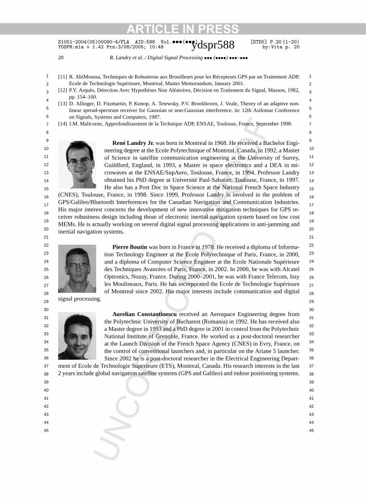
René Landry Jr. was born in Montreal in 1968. He received a Bachelor Enneering degree at the Ecole Polytechnique of Montreal, Canada, in 1992, a Mof Science in satellite communication engineering at the University of SuGuildford, England, in 1993, a Master in space electronics and a DEA incrowaves at the ENSAE/SupAero, Toulouse, France, in 1994. Professor Lobtained his PhD degree at Université Paul-Sabatier, Toulouse, France, inHe also has a Post Doc in Space Science at the National French Space In

(CNES), Toulouse, France, in 1998. Since 1999, Professor Landry is involved in the probGPS/Galileo/Bluetooth Interferences for the Canadian Navigation and Communication InduHis major interest concerns the development of new innovative mitigation techniques for Gceiver robustness design including those of electronic inertial navigation system based on loMEMs. He is actually working on several digital signal processing applications in anti-jammininertial navigation systems.

Pierre Boutin was born in France in 1978. He received a diploma of Informtion Technology Engineer at the Ecole Polytechnique of Paris, France, inand a diploma of Computer Science Engineer at the Ecole Nationale Supédes Techniques Avancées of Paris, France, in 2002. In 2000, he was with AOptronics, Nozay, France. During 2000–2001, he was with France Telecomles Moulineaux, Paris. He has incorporated the Ecole de Technologie Supéof Montreal since 2002. His major interests include communication and d

signal processing.

Aurelian Constantinescu received an Aerospace Engineering degree fthe Polytechnic University of Bucharest (Romania) in 1992. He has receiveda Master degree in 1993 and a PhD degree in 2001 in control from the PolyteNational Institute of Grenoble, France. He worked as a post-doctoral reseaat the Launch Division of the French Space Agency (CNES) in Evry, Francthe control of conventional launchers and, in particular on the Ariane 5 launSince 2002 he is a post-doctoral researcher in the Electrical Engineering D

ment of Ecole de Technologie Superieure (ETS), Montreal, Canada. His research interests in2 years include global navigation satellite systems (GPS and Galileo) and indoor positioning sy

UN

CO

R

39

40

41

42

43

44

45

Documents

New anti-jamming technique for GPS and GALILEO …New anti-jamming technique for GPS and GALILEO receivers using adaptive FADP ﬁlter René Landry Jr.∗, Pierre Boutin, Aurelian