Neutrosophic Optimization - University of New Mexicofs.unm.edu/NeutrosophicOptimizationStructuralDesigns.pdf · 2019-10-23 · Mridula Sarkar Tapan Kumar Roy [email protected] [email protected]

Mridula Sarkar Tapan Kumar Roy

Florentin Smarandache

Neutrosophic Optimizationand its Application on Structural Designs

Mridula SarkarTapan Kumar Roy

[email protected]

[email protected][email protected]


Department of Mathematics, Indian Institute of Engineering Science and Technology, Shibpur, P.O-Botanic Garden, Howrah-711103, West Bengal, India.

Department of Mathematics, University of New Mexico, Gallup Campus, USA.

Neutrosophic Optimization

and its Application on Structural Designs

Mridula SarkarTapan Kumar Roy


Brussels, 2018

mailto:[email protected]

mailto:[email protected]

CONTENTS

Chapter-1 1.1

Basic Notions and Neutrosophic Optimization…………....……….1 Overview……………………………………………………………………….…..1

1.2 Neutrosophic Set…………………………………...………………………….........2 1.3 Single Valued Neutrosophic Set…………………………………….………...........2 1.4 Complement of Neutrosophic Set……………………………….………………….3 1.5 Containment………………………………………………………………...………3 1.6 Equality of Two Neutrosophic Sets…………………………………………..…….4 1.7 Union of Neutrosophic Sets…………………………………………………...…..4 1.8 Intersection of Neutrosophic Sets………………………………..….................…4 1.9 Difference of two single valued Neutrosophic Set…………………………………5 1.10 Normal Neutrosophic Set………………………………………………………....6 1.11 Convex Neutrosophic Set……………………...…………………………….…...6 1.12 Single Valued Neutrosophic Number(SVNN)…………………………..........…6 1.13 Generalized Triangular Neutrosophic Number(GTNN)…………………………..7 1.14 , , Cut of Single Valued Triangular Neutrosophic Number(SVTNN)…....8 1.15 Ranking of Triangular Neutrosophic Number……………………………..…….....8 1.16 Nearest Interval Approximation for Neutrosophic Number……………...............11 1.17 Decision Making in Imprecise Environment……………………………….…..…12

1.18 Single-Objective Neutrosophic Geometric Programming…………………….….13 1.19 Numerical Example of Neutrosophic Geometric Programming…………………..15 1.20 Application of Neutrosophic Geometric Programming in Gravel Box Design

Problem…………………………………………….………………………………17 1.21 Multi-Objective Neutrosophic Geometric Programming Problem………………..18 1.22 Definition: Neutrosophic Pareto(or NS Pareto) Optimal Solution……….………..22 1.23 Theorem 1…………………………………………………………...……………22 1.24 Theorem 2…………………………………………………….…………………..23 1.25 Illustrated Numerical Example……………………………………………………24 1.26 Application of Neutrosophic Optimization in Gravel Box Design Problem……..26 1.27 Multi-Objective Neutrosophic Linear Programming Problem (MOLPP)…….......27 1.28 Production Planning Problem……..………………………………………………39

1.29 Neutrosophic Optimization (NSO)Technique to two type Single-Objective

Minimization Type Nonlinear Programming (SONLP)Problem………………...42

1.30 Neutrosophic Optimization Technique to solve Minimization Type Multi Objective Non-linear Programming Problem for Linear Membership Function...55

1.31 Illustrated Numerical Example…………………………………….……………..63 1.32 Application of Neutrosophic Optimization in Riser Design Problem……………63 1.33 Neutrosophic Optimization(NSO) Technique to Solve Minimization Type Multi

Objective Non-linear Programming Problem(MONLP)……………………...….65

1.34 Neutrosophic Goal Programming(NGP)…………………………………………74

1.35 Theorem on Generalized Goal Programming………………………………….…76

I

1.36 Generalized Neutrosophic Goal Programming(GNGP)………………………….78

1.37 Application of Neutrosophic Goal Programming to Bank Three Investment

Problem……………………………………………………………………………80

1.38 Numerical Example………………………………………………………………82 1.39 Neutrosophic Non-linear Programming (NNLP) Optimization to solve

Parameterized Multi-objective Non-linear Programming Problem (PMONLP)…83

1.40 Neutrosophic Optimization Technique(NSO) to solve Parametric Single-Objectiv

Non-linear Programming Problem (PSONLP)…………………………………..88

Chapter-2 Structural Design Optimization……………………………………………94 2.1 S.I Unit Prefixes …………………………………...………………………...….96 2.2 Conversion of U.S Customary Units to S.I Units……………………………….96 2.3 Design Studies…………………………………………………………………..97

2.3.1 Two-Bar Truss(Model-I)………………………………………….….97 2.3.2 Three-Bar Truss(Model-II)……………………………………...……99 2.3.3 Design Criteria for Thickness Optimization……………………......104

2.3.4 Welded Beam Design Formulation……………………………….109

Chapter-3 Truss Design Optimization using Neutrosophic Optimization Technique:A Comparative Study…………………………………………………….115

3.1 General Formulation of Single-objective Structural Model……………..………...116 3.2 Neutrosophic Optimization Technique to Solve Single-objective Structural

Optimization Problem (SOSOP)………………………………………..….117 3.3 Numerical Solution of Two Bar Truss Design using Single Objective NSO

Technique…………………………………………………………………...128 3.4 Conclusion…………………………………………………………………………136

Chapter-4 Multi-Objective Neutrosophic Optimization Technique and its Application to Structural……………………………………………………………138

4.1 General form of Multi-Objective Truss Design Model………………………....…139 4.2 Solution of Multi-objective Structural Optimization Problem (MOSOP) by

Neutrosophic Optimization Technique……………………………………...140 4.3 Numerical Solution of Solution of Multi-objective Structural Optimization

Problem (MOSOP) by Neutrosophic Optimization Technique……………..147 4.4 Conclusion ………………………………………………………………….....….155

Chapter-5 Optimization of Welded Beam Structure using Neutrosophic OptimizationTechnique: A Comparative Study……………………………………………..156

5.1 Welded Beam Design (WBD)and its Optimization in Neutrosophic

II

Environment…………………………………………………...…………….....158

5.2.1 Crisp Formulation of WBD……………………………………..…..159 5.2.2 WBD Formulation in Neutrosophic Environment……………….....161 5.2.3 Optimization of WBD in Neutrosophic Environment……………....162

5.2 Numerical Solution of WBD by Single Objective Neutrosophic Optimization Technique…………………………………………………………………..…167

5.3 Conclusion…………………………………………………………...…...……....173 Chapter-6 Multi-Objective Welded Beam Optimization using Neutrosophic Optimization

Technique: A Comparative Study………………………………………………175

6.1 General Form of Multi-Objective Welded Beam Design(MOWBD)…………......176 6.2 Solution of Multi-Objective Welded Beam Design (MOWBD) Problem by

Neutrosophic Optimization(NSO) Technique………………………………177 6.3 Numerical Solution of Welded Beam Design using Multi-Objective

Neutrosophic Optimization Technique………………………………...……185 6.4 Conclusion..………………………………………………………………………..197

Chapter-7 Multi-Objective Welded Beam Optimization using Neutrosophic Goal Programming Technique………………………………………..…………...…..198

7.1 General Formulation of Multi-objective Welded Beam Design……….............…200 7.2 Generalized Neutrosophic Goal Optimization Technique to Solve Multi-

objective Welded Beam Optimization Problem (MOWBP)……………..…201 7.3 Numerical Solution of Welded Beam Design by GNGP, based on Different

Operator……………………………………………………………………..204 7.4 Conclusion………………………………………………………………………....211

Chapter-8 Truss Design Optimization with Imprecise Load and Stress in NeutrosophicEnvironment…………………………………………………………………….212

8.1 Multi-Objective Structural Design Formulation…………………………..213

8.2 Parametric Neutrosophic Optimization Technique to Solve Multi-Objective Structural Optimization Problem………………………………………...…214

8.3 Numerical Solution of Three Bar Truss Design using Parametric Neutrosophic Optimization Technique……………………………………218

8.4 Conclusion…………………………………………………………….....…227

Chapter-9 Optimization of Welded Beam with Imprecise Load and Stress byParameterized Neutrosophic Optimization Technique…………….…..229

9.1 General Formulation of Single-Objective Welded Beam Design……………....…230 9.2 NSO Technique to Optimize Parametric Single-Objective Welded Beam

Design(SOWBD)……………………………………………………………231 9.3 Numerical Solution of Parametric Welded Beam Design Problem by NSO

Technique………………………………………………………………..….234 9.4 Conclusion……………………………………………………………...………….242

Chapter-10 Optimization of Thickness of Jointed Plain Concrete Pavement UsingNeutrosophic Optimization Technique…………….…………………...…243

10.1 Formulation for Optimum JPCP Design…………………………………....244

III

10.1.1 Design input parameters…………………...………………………..245 10.1.2 Design method………………………………..…………………….245

10.2 Neutrosophic Optimization……………………………………………..…..248 10.3 Numerical Illustration of Optimum JPCP Design based on IRC:58-2002…251 10.4 Conclusion………………………..………………………………………....254

Chapter-11 Multi-Objective Structural Design Optimization Based on NeutrosophicGoal Programming Technique………………………………………..…...………….256 11.1 Multi-Objective Structural Model………………………………………......257 11.2 Solution of Multi-objective Structural Optimization Problem (MOSOP) by

Generalized Neutrosophic Goal Optimization Technique…..…………...…258 11.3 Numerical Illustration………………………………………...…………….261 11.4 Conclusion……………………………………………………………......…267

Chapter-12 Multi-objective Cylindrical Skin Plate Design Optimization based onNeutrosophic Optimization Technique…………………………………………...….269

12. 1 Multi-Objective Structural Model Formulation…………………………......270

12. 2 Solution of Multi-objective Structural Optimization Problem (MOSOP) byNeutrosophic Optimization Technique…………………………………..….270

12. 3 Numerical Illustration…………………………………………………...…..271

12. 4 Conclusion……………………………………………………………......…274

Chapter-13 APPENDIX-A……………………………………………………..……….275

13.1 Crisp Set…………………………………………...………………………...….275 13.2 Fuzzy Set……………………..……………………………………………..….275 13.3 Height of a Fuzzy Set………………………………..………………………....276 13.4 Normal Fuzzy Set……………………………………………………………....276 13.5 Cut of Fuzzy Set…………………...…………………………………..…..276 13.6 Union of Two Fuzzy Sets………………………………..…………………..…276 13.7 Intersection of Two Fuzzy Sets………………………………...……………....276 13.8 Convex Fuzzy Set…………………………………………………………..…..277 13.9 Interval Number………………………………………………………….....….277 13.10 Fuzzy Number………...……………………………………………..……..….277

13.10.1 Trapezoidal Fuzzy Number(TrFN)……………………………..…..279 13.11 Cut of Fuzzy Number………………………………………………….….279 13.12 Generalized Fuzzy Number (GFN)………………………………………....….280

13.13 Nearest Interval Approximation of Fuzzy Number………………………...…..281

13.14 Intuitionistic Fuzzy Set……………………..………………………………......282 13.15 , Level Or , Cuts…………………………...……..…………....28313.16 Convex Intuitionistic Fuzzy Set………………………………………...……..283 13.17 Union of Two Intuitionistic Fuzzy Sets…………………………………..…....284

IV

13.18 Intersection of Two Intuitionistic Fuzzy Sets………………………………..…284 13.19 Generalized Intuitionistic Fuzzy Number(GIFN)…….…………………....…..284 13.20 Generalized Triangular Intuitionistic Fuzzy Number(GTIFN)…...……………284 13.21 Level Set or Cut of Intuitionistic Fuzzy Number………...……………285 13.22 Arithmetic Operation of Triangular Intuitionistic Fuzzy Number (TIFN)…......285 13.23 Nearest Interval Approximation for Intuitionistic Fuzzy Number…………......286 13.24 Parametric Interval Valued Function…………………………….………..…...287 13.25 Ranking of Triangular Intuitionistic Fuzzy Number…………………………...288

Chapter-14 APPENDIX-B……………………………………………………………...29014.1 Geometric Programming(GP) Method…………………………………….…...290 14.2 Posynomial Geometric Programming Problem……………………………….291 14.3 Signomial Geometric Programing Problem…………………………..……….292 14.4 Fuzzy Geometric Programming (FGP) ………………………………………..293 14.5 Numerical Example of Fuzzy Geometric Programming……………………….295 14.6 Intuitionistic Fuzzy Geometric Programming………………………………….297 14.7 Fuzzy Decision Making……………………………………………..…….......301 14.8 Additive Fuzzy Decision………………………………………………….……301 14.9 Intuitionistic Fuzzy Optimization(IFO) Technique to solve Minimization Type

Single Objective Non-linear Programming (SONLP) Problem ……...…….....302 14.10 Fuzzy Non-linear Programming (FNLP) Technique to Solve Multi-Objective

Non Linear Programming (MONLP) problem……………………………….....306 14.11 An Intuitionistic Fuzzy(IF) Approach for Solving Multi-Objective Non-Linear Programming(MONLP) Problem with Non-linear membership and Non-linear

Non-membership Function……………………………………………….……..308 14.12 Intuitionistic Fuzzy Non-linear Programming (IFNLP) Optimization to solve Parametric Multi-Objective Non-linear Programming Problem (PMONLP)…………...…………………………………………………………..311 14.13 Fuzzy and Intuitionistic Fuzzy Non-linear Programming (IFNLP) Optimization to solve Parametric Single-Objective Non-linear Programming (PSONLP) Problem…………………………………………………………....…316

Bibiliography…………………………………………………………………….322

V

PREFACE

In the real world, uncertainty or vagueness is prevalent in engineering and management

computations. Commonly, such uncertainties are included in the design process by

introducing simplified hypothesis and safety or design factors. In case of structural and

pavement design, several design methods are available to optimize objectives. But all such

methods follow numerous monographs, tables and charts to find effective thickness of

pavement design or optimum weight and deflection of structure calculating certain loop of

algorithm in the cited iteration process. Most of the time, designers either only take help of a

software or stop the cited procedure even after two or three iterations. As for example, the

finite element method and genetic algorithm type of crisp optimization method had been

applied on the cited topic, where the values of the input parameters were obtained from

experimental data in laboratory scale. But practically, above cited standards have already

ranged the magnitude of those parameters in between maximum to the minimum values. As

such, the designer becomes puzzled to select those input parameters from such ranges which

actually yield imprecise parameters or goals with three key governing factors i.e. degrees of

acceptance, rejection and hesitancy, requiring fuzzy, intuitionistic fuzzy, and neutrosophic

optimization.

Therefore, the problem of structural designs, pavement designs, welded beam designs

are firstly classified into single objective and multi-objective problems of structural systems.

Then, a mathematical algorithm - e.g. Neutrosophic Geometric Programming, Neutrosophic

Linear Programming Problem, Single Objective Neutrosophic Optimization, Multi-objective

Neutrosophic Optimization, Parameterized Neutrosophic Optimization, Neutrosophic Goal

Programming Technique - has been provided to solve the problem according to the nature of

impreciseness that exists in the problem.

Thus, we provide in this book a solution which is hardly presented in the scientific

literature regarding structural optimum design, pavement optimum design, welded beam

optimum design, that works in imprecise environment i.e. in neutrosophic environment.

The objective of the book is not only to study the concept of neutrosophic set, single valued

neutrosophic set, complement of neutrosophic set, union of neutrosophic set, intersection of

neutrosophic set, generalized fuzzy number, triangular fuzzy number, normal neutrosophic

VI

set, convex neutrosophic set, single valued neutrosophic number, generalized triangular

neutrosophic number and their properties, but also to fulfil the criteria of specification of such

concepts from a technical point of view. The second objective of the book is the

identification of impreciseness that is involved in real life engineering design problems, such

as in various structural design problems, welded beam designs and pavement designs

problems. For example, they are often exhibit in the form of applied load, stresses, deflection

in the test problem, therefore we employ ultimate development of mathematical algorithm

using neutrosophic set theory to optimize various truss, welded beam, pavement design

problems in neutrosophic environment.

In the following chapters, some mathematical optimization methods on neutrosophic set

theory have been studied and the results have been compared agaist Fuzzy and Intuitionistic

Fuzzy Optimization methods. Some structural models like two-bar, three bar truss, welded

beam design, jointed plain concrete pavement are formulated and solved in fuzzy,

intuitionistic fuzzy or neutrosophic environments. The proposed thesis has been divided into

following chapters:

In the First chapter, the basic concepts and definitions of Neutrosophic set, Single Valued

Neutrosophic Set (SVNS), complement of Neutrosophic Set, union of Neutrosophic Set,

intersection of Neutrosophic Set, Normal Neutrosophic Set, Convex Neutrosophic Set, Single

Valued Neutrosophic Number (SVNN), Generalized Triangular Neutrosophic Number

(GTNN) are given. Also, in this chapter, some basic methodologies - such as neutrosophic

linear programming, neutrosophic geometric programming, neutrosophic optimization

technique to solve minimization type single objective nonlinear programming problem,

neutrosophic optimization technique to solve minimization type nonlinear programming

problem, solution of multi-objective welded beam optimization problem by generalized

neutrosophic goal programming technique, neutrosophic non-linear programming

optimization to solve parameterized multi-objective nonlinear programming problem,

neutrosophic optimization technique to solve parametric single objective nonlinear

programming problem - have been discussed to solve several trusses, welded beam optimum

and jointed plain concrete pavement designs.

VII

In the Second chapter, an introduction of structural design optimization, conversion between

U.S customary units and S.I units, S.I. unit prefixes, formulation of truss design, some welded

beam designs and pavement designs are presented.

In the Third Chapter, we take into consideration a neutrosophic optimization (NSO) approach

for optimizing the design of truss with single objective, subject to a specified set of constraints.

In the Fourth chapter, a multi-objective non-linear neutrosophic optimization (NSO) approach

for optimizing the design of plane truss structure with multiple objectives subject to a specified

set of constraints is explained.

In the Fifth chapter, a Neutrosophic Optimization (NSO) approach is investigated to optimize

the cost of welding of a welded steel beam, where the maximum shear stress in the weld group,

maximum bending stress in the beam, maximum deflection at the tip and buckling load of the

beam are considered as flexible constraints.

In the Sixth chapter, a multi–objective Neutrosophic Optimization (NSO) approach is studied

to optimize the cost of welding and deflection at the tip of a welded steel beam.

In the Seventh chapter, a multi–objective Neutrosophic Goal Optimization (NSGO) approach

with different aggregation method is explored to optimize the cost of welding and deflection

at the tip of a welded steel beam, while the maximum shear stress in the weld group, maximum

bending stress in the beam, and buckling load of the beam are considered as constraints.

In the Eighth Chapter, we employ a neutrosophic mathematical programming to solve a multi-

objective structural optimization problem with imprecise parameters. Generalized Single

Valued Triangular Neutrosophic Numbers (GSVNNs) are assumed imprecise loads and stresses

in a test problem.

In the Ninth chapter, a solution procedure of Neutrosophic Optimization (NSO) is examined

to solve optimum welded beam design with inexact co-efficient and resources. Interval

approximation method is used here to convert the imprecise co-efficient, which is a triangular

neutrosophic number, to an interval number.

In the Tenth chapter, the optimization of thickness of Jointed Plain Concrete Pavement (JPCP)

by following the guidelines of Indian Roads Congress (IRC:58- 2002) in imprecise environment

is studied and solved by neutrosophic optimization technique.

In the Eleventh Chapter, we analyze a multi-objective Neutrosophic Goal Optimization

(NSGO) technique for optimizing the design of three bar truss structure with multiple

objectives, subject to a specified set of constraints.

VIII

In the Twelfth Chapter, we search upon a Neutrosophic Optimization (NSO) approach for

optimizing the thickness and sag of skin plate of vertical lift gate with multi- objective, subject

to a specified constraint.

The Authors

IX

Page 1

CHAPTER 1Basic Notions and Neutrosophic Optimization

1.1 Over view The concept of fuzzy set was introduced by Zadeh in 1965.Since the fuzzy sets and fuzzy

logic have been applied in many real applications to handle uncertainty. The traditional fuzzy

set uses only real value 0,1A x to represent the grade of membership of fuzzy set A

defined on universe X .Sometimes A x itself is uncertain and hard to be defined by a

crisp value. So the concept of interval valued fuzzy sets was proposed to capture the

uncertainty of grade of membership. Interval valued fuzzy sets uses an interval value

,L UA Ax x with 0 1L U

A Ax x to represent the grade of membership of fuzzy

set A . In some applications such as expert system, belief system and information fusion, we

should consider not only the truth membership supported by the evident but also the falsity

membership against by the evident. That is beyond the scope of fuzzy sets and interval valued

fuzzy sets. In 1986 Atanassov introduced the Intuitionistic fuzzy sets which is a

generalization of fuzzy sets and probably equivalent to interval valued fuzzy sets.The

intuitionistic fuzzy sets consider both truth membership iAT x and falsity membership

iAF x with ,iA

T x iAF x 0,1 and 0 1.i iA A

T x F x Intuitionistic fuzzy sets

can only handle incomplete information not the indeterminate information and inconsistent

information which exists commonly belief in system. In intuitionistic fuzzy sets,

indeterminacy is 1 i iA AT x F x by default. For example when we ask the opinion of

expert about certain statement, he or she may be in the position of the possibility that the

statement is true is 0.5 and the statement is false is 0.6 and the degree that he or she is not

sure is 0.2.

In neutrosophic set indeterminacy is quantified explicitly and truth membership,

indeterminacy membership and falsity membership are independent. This assumption is very

important in a lot of situations such as information fusion when we try to combine the data

from different sensors. Neutrosophy was introduced by Smarandache in 1995.”It is a branch

of philosophy which studies the origin, nature and scope of nutralities, as well as their

Page 2

interactions with different ideational spectra”.Neutrosophic Set is a power general framework

which generalizes the concept of the classic set, fuzzy set ,interval valued fuzzy set,

intuitionistic fuzzy set e.t.c. A neutrosophic set nA defined on universe U.

, , nx x T I F A with , ,T I F being real standard or nonstandard subset of 0 ,1 . T

is the degree truth membership function in the set ,nA I is the degree indeterminacy

membership function in the set nA and F is the degree falsity membership function in the set

.nA

The neutrosophic set generalizes the above mensioned sets from philosophical point of view.

From scientific or engineering point of view the neutrosophic set and set theoretic operators

need to be specified. Otherwise, it will be difficult to apply in the real applications. In this

paper, we define neutrosophic set (the set theoretic operators on an instance of neutrosophic

set called SVNS).

1.2 Neutrosophic Set (NS)

Let X be a space of points (objects) with a generic element in X denoted by x i.e. x X . A neutrosophic set nA in X is characterized by truth-membership function nA

Tindeterminacy- membership function nA

I and falsity-membership function nAF , where

, ,n n nA A AT I F are the functions from U to ] 0, 1 [ i.e. , ,n n nA A A

T I F : X ] 0, 1 [ ,that

means , ,n n nA A AT I F are the real standard or non-standard subset of ] 0, 1 [. Neutrosophic set

can be expressed as , , , :n n nn

A A AA x T I F x X . Since , ,n n nA A A

T I F are the subset of ]0, 1 [ , there the sum

, ,n n nA A AT I F lies between 0 and 3 , where 0 = 0 - and 3 = 3 + , >0.

The set nAI may represent not only indeterminacy, but also vagueness, uncertainty,

imprecision, error, contradiction, undefined, unknown, incompleteness, redundancy, etc. In order to catch up vague information, an indeterminacy-membership degree can be split into subcomponents, such as „„contradiction,‟‟ „„uncertainty‟‟, and „„unknown‟‟.

Example 1.

Suppose that 1 2 3, , ,........ .X x x x be the universal set. Let 1A be any neutrosophic set in X.

Then 1A expressed as 1 1 1: .6,.3,.4 :A x x X .

Page 3

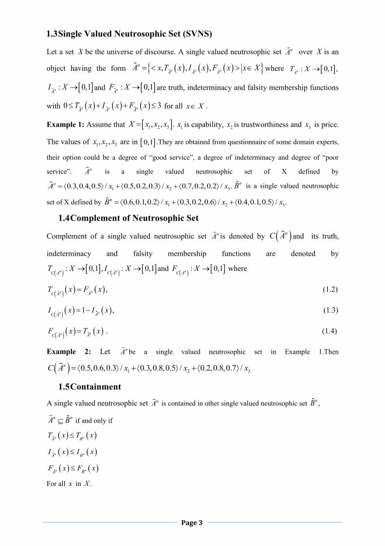
Let a set X be the universe of discourse. A single valued neutrosophic set nA over X is an

object having the form , , ,n n nn

A A AA x T x I x F x x X where : 0,1 ,nA

T X

: 0,1nAI X and : 0,1nA

F X are truth, indeterminacy and falsity membership functions

with 0 3n n nA A AT x I x F x for all x X .

Example 1: Assume that 1 2 3, , .X x x x 1x is capability, 2x is trustworthiness and 3x is price.

The values of 1 2 3, ,x x x are in 0,1 .They are obtained from questionnaire of some domain experts,

their option could be a degree of “good service”, a degree of indeterminacy and degree of “poor

service”. nA is a single valued neutrosophic set of X defined by

1 2 30.3,0.4,0.5 / 0.5,0.2,0.3 / 0.7,0.2,0.2 / .nA x x x nB is a single valued neutrosophic

set of X defined by 1 2 30.6,0.1,0.2 / 0.3,0.2,0.6 / 0.4,0.1,0.5 / .nB x x x

1.4 Complement of Neutrosophic Set

Complement of a single valued neutrosophic set nA is denoted by nC A and its truth,

indeterminacy and falsity membership functions are denoted by

: 0,1 , : 0,1n nC A C AT X I X and

: 0,1nC AF X where

,nn AC AT x F x (1.2)

1 ,nn AC AI x I x (1.3)

nn AC AF x T x . (1.4)

Example 2: Let nA be a single valued neutrosophic set in Example 1.Then

1 2 30.5,0.6,0.3 / 0.3,0.8,0.5 / 0.2,0.8,0.7 /nC A x x x

1.5 Containment

A single valued neutrosophic set nA is contained in other single valued neutrosophic set ,nB

n nA B if and only if

n nA BT x T x

n nA BI x I x

n nA BF x F x

For all x in .X

1.3 Single Valued Neutrosophic Set (SVNS)

Page 4

Note that by definition of containment, X is partial order but not linear order. For example let nA and nB be the single valued neutrosophic sets defined in example 1.Then nA is not contained in nB and nB is not contained in nA

1.6 Equality of Two Neutrosophic Sets

Two single valued neutrosophic sets nA and nB are said to be equal and written as n nA B if

and only if n nA B and n nA B

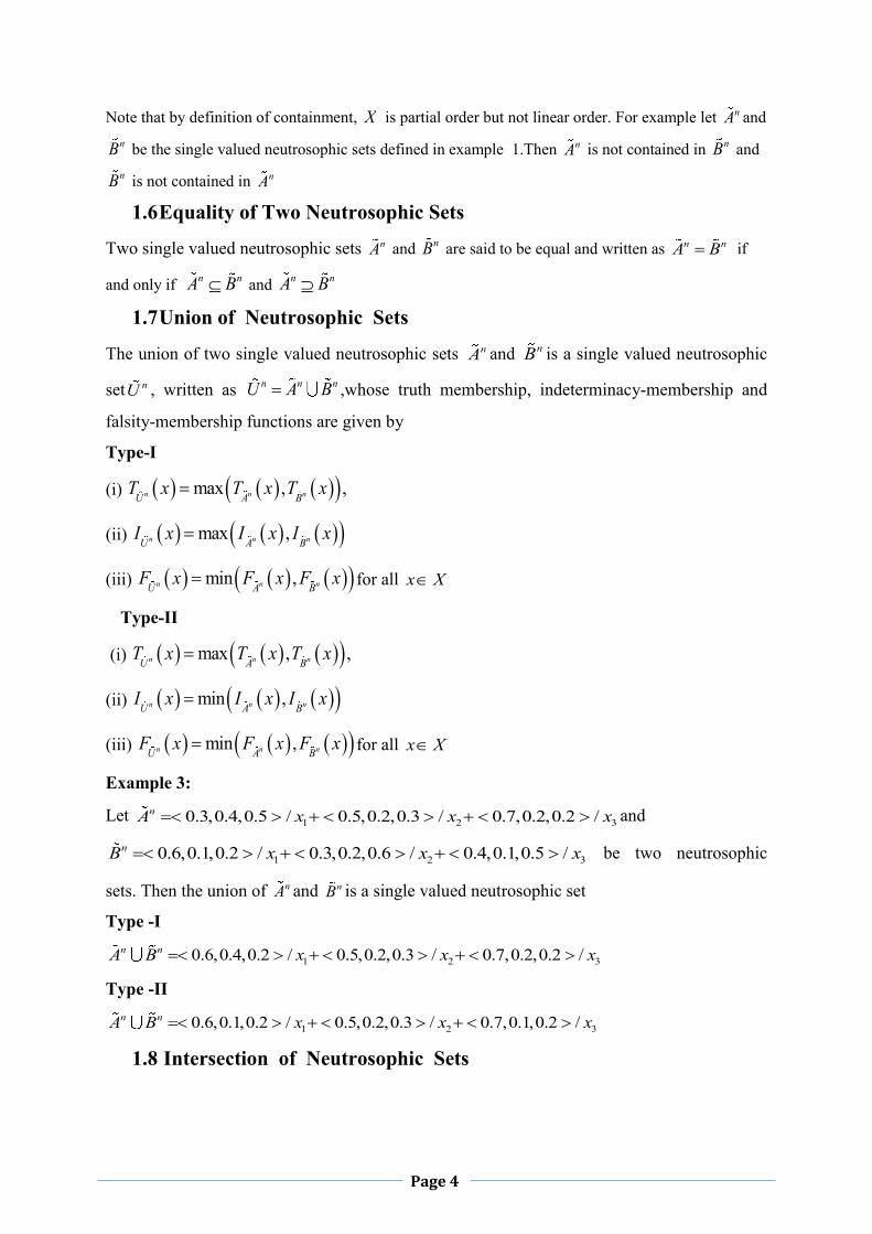
1.7 Union of Neutrosophic Sets

The union of two single valued neutrosophic sets nA and nB is a single valued neutrosophic

set nU , written as n n nU A B ,whose truth membership, indeterminacy-membership and

falsity-membership functions are given by

Type-I

(i) max , ,n n nU A BT x T x T x

(ii) max ,n n nU A BI x I x I x

(iii) min ,n n nU A BF x F x F x for all x X

Type-II

(i) max , ,n n nU A BT x T x T x

(ii) min ,n n nU A BI x I x I x

(iii) min ,n n nU A BF x F x F x for all x X

Example 3:

Let 1 2 30.3,0.4,0.5 / 0.5,0.2,0.3 / 0.7,0.2,0.2 /nA x x x and

1 2 30.6,0.1,0.2 / 0.3,0.2,0.6 / 0.4,0.1,0.5 /nB x x x be two neutrosophic

sets. Then the union of nA and nB is a single valued neutrosophic set

Type -I

1 2 30.6,0.4,0.2 / 0.5,0.2,0.3 / 0.7,0.2,0.2 /n nA B x x x

Type -II

1 2 30.6,0.1,0.2 / 0.5,0.2,0.3 / 0.7,0.1,0.2 /n nA B x x x

1.8 Intersection of Neutrosophic Sets

Page 5

The intersection of two single valued neutrosophic sets nA and nB is a single valued

neutrosophic set nE , written as n n nE A B ,whose truth membership, indeterminacy-

membership and falsity-membership functions are given by

Type-I

(i)

min , ,n n nE A BT x T x T x

(ii)

min ,n n nE A BI x I x I x

(iii)

max ,n n nE A BF x F x F x for all x X

Type-II

(i)

min , ,n n nE A BT x T x T x

(ii)

max ,n n nE A BI x I x I x

(iii)

max ,n n nE A BF x F x F x for all x X

Example 4:

Let 1 2 30.3,0.4,0.5 / 0.5,0.2,0.3 / 0.7,0.2,0.2 /nA x x x and

1 2 30.6,0.1,0.2 / 0.3,0.2,0.6 / 0.4,0.1,0.5 /nB x x x be two neutrosophic

sets. Then the union of nA and nB is a single valued neutrosophic set

Type -I

1 2 30.3,0.1,0.5 / 0.3,0.2,0.6 / 0.4,0.1,0.5 /n nA B x x x

Type -II

1 2 30.3,0.4,0.5 / 0.3,0.2,0.6 / 0.4,0.2,0.5 /n nA B x x x

1.9 Difference of Two Single Valued Neutrosophic set

The difference of two single valued neutrosophic set ,nD written as / ,n n nD A B whose

truth-membership,indeterminacy membership and falsity membership functions are related to

those of nA and nB can be defined by

(i)

min , ,n n nD A BT x T x T x

(ii)

min ,1n n nD A BI x I x I x

(iii)

max ,n n nD A BF x F x F x for all x X

Page 6

Example 5: Let nA and nB be a single valued neutrosophic set in Example 1.Then

1 2 30.2,0.4,0.6 / 0.5,0.2,0.3 / 0.5,0.2,0.4 /nD x x x

1.10 Normal Neutrosophic Set

A single valued neutrosophic set , , ,n n nn

A A AA x T x I x F x x X is called

neutrosophic normal if there exists at least three points 0 1 2, ,x x x X such that 0 1nAT x

1 1,nAI x 2 1nA

F x .

1.11 Convex Neutrosophic Set


A A AA x T x I x F x x X is a subset of the

real line called neut-convex if for all 1 2,x x and 0,1 the following conditions are

satisfied.

1. 1 2 1 21 min ,n n nA A AT x x T x T x

2. 1 2 1 21 max ,n n nA A AI x x I x I x

3. 1 2 1 21 max ,n n nA A AF x x F x F x

i.e nA is neut-convex if its truth membership function is fuzzy convex, indeterminacy

membership function is fuzzy concave and falsity membership function is fuzzy concave.

1.12 Single Valued Neutrosophic Number(SVNN)


A A AA x T x I x F x x X ,subset of a real

line ,is called generalised neutrosophic number if

1. nA is neut- normal.

2. nA is neut- convex.

3. nAT x is upper semi-continuous, nA

I x is lower semi continuous and nAF x is lower

semi continuous ,and

4. the support of nA ,i.e .

: 0, 1, 1n n nn

A A AS A x X T I F

(1.5)

is bounded.

Thus for any Single Valued Triangular Neutrosophic Number (TNN)there exists nine

numbers 1 2 3 1 2 3 1 2 3, , , , , , , ,T T I I F Fa a a b b b c c c such that 1 1 1 2 2 2 3 3 3F I T T I Fc b a c b a a b c

Page 7

and six functions , , , , , : 0,1n n n n n nL L L R R R

A A A A A AT x I x F x T x I x F x represent truth,

indeterminacy and falsity membership degree of nA .The three non-decreasing functions

, ,n n nL L L

A A AT x I x F x represent the left side of truth, indeterminacy and falsity membership

functions of SVNN nA respectively. Similarly the three non-increasing functions

, ,n n nR R R

A A AT x I x F x represent the right side of truth ,indeterminacy and falsity

membership functions of SVNN nA respectively. The truth, indeterminacy and falsity

membership functions of SVNN nA can be defined in the following way

1 2

2 3 ;0

n

n n

L TAR T

A A

T x if a x aT x T x if a x a

otherwise

(1.6)

1 2

2 3

0

n

n n

L IAR I

A A

I x if b x bI x I x if b x b

otherwise

(1.7)

1 2

2 3

0

n

n n

L FAR F

A A

F x if c x cF x F x if c x c

otherwise

(1.8)

The sum of three independent membership degree of SVNN nA lie between the interval

0,3 .i.e 0 3n n nR R R n

A A AT x I x F x x A . (1.9)

1.13 Generalized Triangular Neutrosophic Number(GTNN) A generalized single valued triangular neutrosophic number nA with the set of parameters

1 1 1 2 2 2 3 3 3F I T T I Fc b a c b a a b c denoted as

1 2 3 1 2 3 1 2 3, , ; , , , ; , , ;n T T I I F Fa a aA a a a w b b b c c c is the set of real numbers .The truth

membership, indeterminacy membership and falsity membership functions of nA can be

defined as follows

11 2

2 1

2

32 3

3 2

0

n

TT

a T

aA T

Ta T

x aw for a x aa a

w for x aT

a xw for a x aa a

otherwise

(1.10)

Page 8

11 2

2 1

2

32 3

3 2

0

n

II

a I

aA I

Ia I

x b for b x bb b

for x bI

x b for b x bb b

otherwise

(1.11)

11 2

2 1

2

32 3

3 2

0

n

FF

a F

aA F

Fa F

x c for c x cc c

for x cF

x c for c x cc c

otherwise

(1.12)

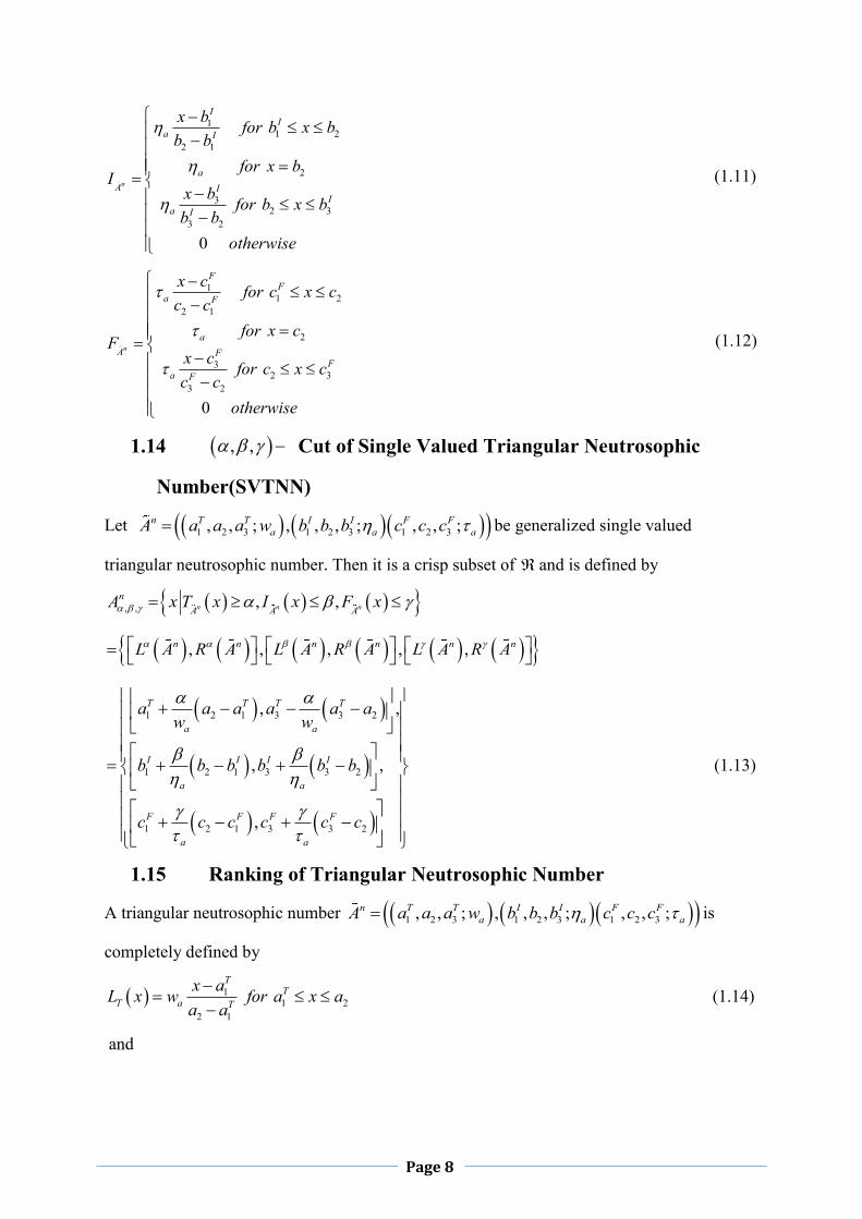
1.14 , , Cut of Single Valued Triangular Neutrosophic

Number(SVTNN)

Let 1 2 3 1 2 3 1 2 3, , ; , , , ; , , ;n T T I I F Fa a aA a a a w b b b c c c be generalized single valued

triangular neutrosophic number. Then it is a crisp subset of and is defined by

, , , ,n n nn

A A AA x T x I x F x

, , , , ,n n n n n nL A R A L A R A L A R A

1 2 1 3 3 2

1 2 1 3 3 2

1 2 1 3 3 2

, ,

, ,

,

T T T T

a a

I I I I

a a

F F F F

a a

a a a a a aw w

b b b b b b

c c c c c c

(1.13)

1.15 Ranking of Triangular Neutrosophic Number

A triangular neutrosophic number 1 2 3 1 2 3 1 2 3, , ; , , , ; , , ;n T T I I F Fa a aA a a a w b b b c c c is

completely defined by

11 2

2 1

TT

T a T

x aL x w for a x aa a

(1.14)

and

Page 9

32 3

3 2

;T

TT a T

a xR x w for a x aa a

(1.15)

11 2

2 1

II

I a I

x bL x for b x bb b

(1.16)

and

32 3

3 2

;I

II a I

x bR x for b x bb b

(1.17)

11 2

2 1

FF

F a F

x cL x for c x cc c

(1.18)

and 32 3

3 2

FF

F a F

x cR x for c x cc c

(1.19)

.The inverse functions can be analytically expressed as

11 2 1 ;T T

Ta

hL h a a aw

(1.20)

13 3 2 ;T T

Ta

hR h a a aw

(1.21)

1

1 2 1 ;I II

a

hL h b b b

(1.22)

13 3 2 ;I I

Ia

hR h b b b

(1.23)

11 2 1F F

Fa

hL h c c c

(1.24)

And

13 3 2F F

Fa

hR h c c c

(1.25)

Now left integral value of truth membership ,indeterminacy membership and falsity

membership functions of nA are

1

1 21

0

2 12T

Tan

L Ta

w a aV A L h

w

(1.26)

and

1

1 21

0

2 12I

anL I

a

b bV A L h

(1.27)

Page 10

and

1

1 21

0

2 12F

anL I

a

c cV A L h

(1.28)

respectively

and right integral value of truth, indeterminacy and falsity membership functions are

1

3 21

0

2 1,

2T

Tan

R Ta

w a aV A R h

w

(1.29)

1

3 21

0

2 12I

Ian

R Ia

b bV A R h

(1.30)

and

1

3 21

0

2 12F

Fan

R Fa

c cV A R h

(1.31)

respectively.

The total integral value of the truth membership functions is

2 3 13 2 1 2 2 1 12 1 2 1

1 ; 0,12 2 2

T TT Taa an

Ta a a

a w a aw a a w a aV A

w w w

(1.32)

The total integral value of indeterminacy membership functions is

3 2 1 2 2 32 1 2 1 1 2 2 2 11 ; 0,1

2 2 2

I Ia a an

Ia a a

b b b b b bV A

(1.33)

The total integral value of falsity membership functions is

3 2 1 2 2 32 1 2 1 1 2 2 2 11 ; 0,1

2 2 2

F Ia a an

Fa a a

c c c c c cV A

(1.34)

Let 1 2 3 1 2 3 1 2 3, , ; , , , ; , , ;n T T I I F Fa a aA a a a w b b b c c c and

1 2 3 1 2 3 1 2 3, , ; , , , ; , , ;n T T I I F Fb b bB e e e w f f f g g g be two generalized triangular

neutrosophic number then the following conditions hold good

i) If ,n nT TV A V B ,n n

I IV A V B and n nF FI A I B for

, , 0,1 then n nA B

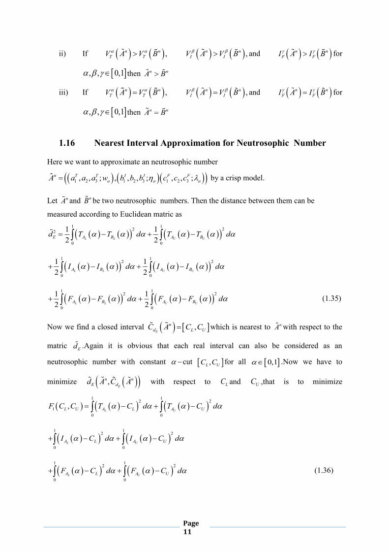
Page 11

ii) If ,n nT TV A V B ,n n


, , 0,1 then n nA B

iii) If ,n nT TV A V B ,n n


, , 0,1 then n nA B

1.16 Nearest Interval Approximation for Neutrosophic Number

Here we want to approximate an neutrosophic number

1 2 3 1 2 3 1 2 3, , ; , , , ; , , ;n T T I I F Fa a aA a a a w b b b c c c by a crisp model.

Let nA and nB be two neutrosophic numbers. Then the distance between them can be

measured according to Euclidean matric as

1 1 222

0 0

1 12 2L L U UE A B A Bd T T d T T d

1 1 22

0 0

1 12 2L L U UA B A BI I d I I d

1 1 22

0 0

1 12 2L L U UA B A BF F d F F d

(1.35)

Now we find a closed interval ,

E

nd L UC A C C which is nearest to nA with respect to the

matric Ed .Again it is obvious that each real interval can also be considered as an

neutrosophic number with constant cut ,L UC C for all 0,1 .Now we have to

minimize ,E

n nE dd A C A with respect to LC and UC ,that is to minimize

1 1 22

10 0

,L UL U A L A UF C C T C d T C d

1 1 22

0 0L UA L A UI C d I C d

1 1 22

0 0L UA L A UF C d F C d

(1.36)

Page 12

With respect to LC and UC . We define partial derivatives

11

0

,2 6

L L L

L UA A A L

L

F C CT I F d C

C

(1.37)

11

0

,2 6

U U U

L UA A A U

U

F C CT I F d C

C

(1.38)

And then we solve the system

1 ,0,L U

L

F C CC

(1.39)

1 ,0L U

U

F C CC

. (1.40)

The solution is

1

0

;3

L L LA A AL

T I FC d

(1.41)

1

0 3U U LA A A

U

T I FC d

(1.42)

Since

2 21 1

2

2 21 1

2

, ,6 0

det 36 00 6, ,

L U L U

L L U

L U L U

U L U

F C C F C CC C C

F C C F C CC C C

(1.43)

then LC UC mentioned above minimize 1 ,L UF C C . The nearest interval of the neutrosophic

number nA with respect to the matric Ed is

1 1

0 0

,3 3

U U UL L L

E

A A AA A And

T I FT I FC A d d

(1.44)

3 3 3 2 3 3 2 3 21 1 1 2 1 2 1 2 1 ,3 6 6 6 3 6 6 6

T I F T I FT I F T I F

a a a a a a

a b c a a b b c ca b c a a b b c cw w

1.17 Decision Making in Neutrosophic Environment

Decision making is a process of solving the problem in involving pursuing the goals under

constraints. The outcome is a decision which should in an action. Decision making plays an

Page 13

important role in an economic and business, management sciences, engineering and

manufacturing, social and political science, biology and medicine, military, computer science

etc. It is difficult process due to factors like incomplete information which tend to be

presented in real life situations. In the decision making process our main target is to find the

value from the selected set with highest degree of membership in the decision set and these

values support the goals under constraints only. But there may arise situations where some

values selected from the set cannot support i.e such values strongly against the goals under

constraints which are non-admissible. In this case we find such values from the selected set

with least degree of non-membership in the decision sets. Intuitionistic fuzzy sets only can

handle incomplete information not the indeterminate information and inconsistent

information which exists commonly belief in system. In neutrosophic set, indeterminacy is

quantified explicitly and truth membership, indeterminacy membership and falsity

membership are independent. So it is natural to adopt for that purpose the value from

selected set with highest degree of truth membership ,indeterminacy membership and least

degree of falsity membership in the decision set. These factors indicate that a decision

making process takes place in neutrosophic environment.

1.18 Single-Objective Neutrosophic Geometric Programming

Let us consider a Neutrosophic Geometric Programming Problem as

(P1. 1)

0

nMin f x (1.45)

Subject to

nj jf x b 1,2,..,j m (1.46)

0x (1.47)

Here the symbol “ n ” denotes the neutrosophic version of “ ”.Now for Neutrosophic geometric programming linear truth,falsity and indeterminacy membership functions can be represented as follows

0

'0 '

' 0

'

1

0

j j

j jj j j j j

j j

j j

if f x ff f x

f x if f f x ff f

if f x f

(1.48)

Page 14

0,1,2,...,j m

' ''

' ''' '' '

''

'

1

0

j j j

j j jj j j j j j

j

j j

if f x f f

f x f ff x if f f f x f

fif f x f

(1.49)

0,1,2,...,j m

0

' '''0 ' '''

' ''' 0

' '''

1

0

j j

j j jj j j j j j

j j j

j j j

if f x f

f f f xf x if f f x f f

f f f

if f x f f

(1.50)

Now a Neutrosophic Geometric programming problem(P1.1) with truth ,falsity and indeterminacy membership function can be written as

(P1. 2)

j jMaximize f x (1.51)

j jMinimize f x (1.52)


0,1,2,...,j m

Considering equal importance of all truth,falsity and indeterminacy membership functions and using weighted sum method the above optimization problem reduces to

(P1. 3)

0

m

A j j j j j jj

Maximize V f x f x f x

(1.54)

Subject to

0x (1.55)

The above problem is equivalent to

(P1. 4)

Page 15

' '' ' ' '''

1 ' 0 '' ' ''' 0 '' ' 0 ' '' 00

1 1 1mj j j j j

A jj j j j j j j j j j j j

f f f f fMinimize V f x

f f f f f f f f f f f f

(1.56)

Subject to

1 1

1j

jki

N na

j jk ik i

f x C x

1,2,...,j m (1.57)

0ix 1,2,...,i n (1.58)

Where 0jkC and jkia are all real. 1 2, ,.., .Tnx x x x

The posynomial Geometric Programming problem can be solved by usual geometric programming technique.

1.19 Numerical Example of Neutrosophic Geometric Programming

Consider an Intuitionistic Fuzzy Nonlinear Programing Problem as

(P1. 5)

2 30 1 2 1 2, 2

nMinimize f x x x x (target value 57.87 with tolerance 2.91) (1.59)

Subject to

1 11 1 2 1 2, 6.75f x x x x ( with tolerance 2.91) (1.60)

2 1 2 1 2, 1f x x x x (1.61)

1 2, 0x x

Here linear truth ,falsity and indeterminacy membership functions for fuzzy objectives and constraints goals are

2 31 2

2 32 31 2

0 0 1 2 1 2

2 31 2

1 2 57.8760.78 2, 57.87 2 60.78

2.910 2 60.78

if x xx xf x x if x x

if x x

(1.62)

1 21 2

1 21 21 2

1 1 1 2 1 2

1 21 2

1 6.756.94, 6.75 6.94

0.190 6.94


if x x

(1.63)

Page 16

2 31 2

2 32 31 2

0 0 1 2 1 2

2 31 2

1 2 59.032 59.03, 59.03 2 60.78

1.750 2 60.78


if x x

(1.64)

1 21 2

1 21 21 2

1 1 1 2 1 2

1 21 2

1 6.836.83, 6.83 6.94

0.110 6.94


if x x

(1.65)

2 31 2

2 32 31 2

0 0 1 2 1 2

2 31 2

1 2 57.8759.50 2, 57.87 2 59.50

1.630 2 59.50


if x x

(1.66)

1 21 2

1 21 21 2

1 1 1 2 1 2

1 21 2

1 6.756.88, 6.75 6.88

0.130 6.88


if x x

(1.67)

Based on max-additive operator FGP (P1.5) reduces to

(P1. 6)

1 1 2 31 2 1 2 1 2

1 1 1 1 1 1, 20.19 0.11 0.13 2.91 1.75 1.63AMaximize V x x x x x x

(1.68)

Subject to

2 1 2 1 2, 1f x x x x (1.69)

1 2, 0x x

Neglecting the constant term in the following model we have following crisp geometric programming problem as

(P1. 7)

1 1 2 31 2 1 2 1 2, 22.046 3.057132Maximize V x x x x x x

(1.70)

Subject to

2 1 2 1 2, 1f x x x x (1.71)

Page 17

1 2, 0x x (1.72)

Here DD=4-(2+1)=1

The dual problem of this GP is

01 02 11 12

11 12

11 1201 02 11 12

22.046 3.057132 1 1w w w w

w wMax d w w ww w w w

(1.73)

Such that

01 02 1w w (1.74)

01 02 112 0w w w (1.75)

01 02 122 3 0w w w (1.76)

So 02 011 ;w w 11 012 ;w w 12 013 ;w w (1.77)

01 01 01 01

01

1 2 35 2

01 0101 01 01 01

22.046 3.057132 1 1 5 21 2 3

w w w wwMaximize d w w

w w w w

(1.78)

Subject to

010 1w (1.79)

For optimality, 01

01

0d d w

dw (1.80)

2

01 01 01 01 0122.046 1 2 3 3.057132 5 2w w w w w (1.81)

*01 0.6260958,w *

02 0.3739042,w *11 1.3739042,w *

12 2.3739042,w (1.82)

*1 0.366588,x *

2 0.633411,x (1.83)

* * *0 1 2, 58.56211,f x x * * *

1 1 2, 6.799086,f x x (1.84)

1.20 Application of Neutrosophic Geometric Programming in Gravel Box Design Problem

Gravel Box Problem: A total of 800 cubic meters of gravel is to be ferried across a river on a barrage. A box (with an open top) is to be built for this purpose. After the entire gravel has been ferried, the box is to be discarded. The transport cost of round trip of barrage of box is Rs 1 and the cost of materials of the ends of the box are Rs 20/m2and cost of the material of

Page 18

other two sides and bottom are Rs 10/m2 and Rs 80/m2 respectively.Find the dimension of the gravel box that is to be built for this purpose and the total optimal cost. Let length ,width and height of the box be 1 2 3, ,x m x m x m respectively. The area of the end of the gravel box is

22 3x x m . The area of the sides and bottom of the gravel box are 2

1 3x x m and 21 2x x m

respectively. The volume of the gravel box is 31 2 3 .x x x m Transport cost is Rs

1 2 3

80x x x

.Material

cost is 2 340x x .

So the gravel box problem can be formulated as multi-objective geometric programming problem as

(P1. 8)

1 1 2 3 2 31 2 3

80, , 40Minimize f x x x x xx x x

(1.85)

2 1 2 31 2 3

80, ,Minimize f x x xx x x

(1.86)

Such that

1 2 1 32 4x x x x (1.87)

1 2 3, , 0x x x

(1.88)

Here objective goal is 90(with truth tolerance 8, falsity tolerance 5 and indeterminacy tolerance 5)

And constraint goal

1 1 2 3, , 4f x x x (with truth tolerance 0.9,falsity tolerance 0.5 and indeterminacy tolerance

0.6)

*1 2.4775,x *

2 0.1271,x *3 0.5635,x (1.89)

* * *0 1 2, 76.237,f x x * * *

1 1 2, 4.5856,f x x

1.21 Multi-Objective Neutrosophic Geometric Programming Problem

A multi-objective geometric programming problem can be defined as

(P1. 9)

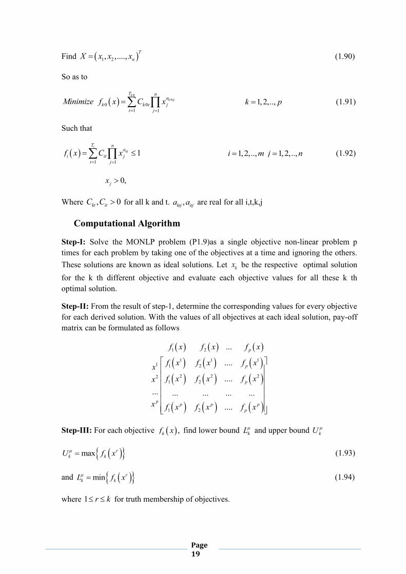
Page 19

Find 1 2, ,...., TnX x x x (1.90)

So as to

0

00 0

1 1

kk tj

T na

k k t jt j

Minimize f x C x

1,2,..,k p (1.91)

Such that

1 1

1i

itj

T na

i it jt j

f x C x

1,2,..,i m 1,2,..,j n (1.92)

0,jx

Where , 0kt itC C for all k and t. ,ktj itja a are real for all i,t,k,j

Computational Algorithm

Step-I: Solve the MONLP problem (P1.9)as a single objective non-linear problem p times for each problem by taking one of the objectives at a time and ignoring the others. These solutions are known as ideal solutions. Let kx be the respective optimal solution for the k th different objective and evaluate each objective values for all these k th optimal solution.

Step-II: From the result of step-1, determine the corresponding values for every objective for each derived solution. With the values of all objectives at each ideal solution, pay-off matrix can be formulated as follows

1 2

1 1 11 1 2

2 2 221 2

1 2

...

....

....... ... ... ... ...

....

p

p

p

p p p pp

f x f x f x

f x f x f xxf x f x f xx

x f x f x f x

Step-III: For each objective ,kf x find lower bound kL and upper bound kU

max rk kU f x (1.93)

and min rk kL f x (1.94)

where 1 r k for truth membership of objectives.

Page 20

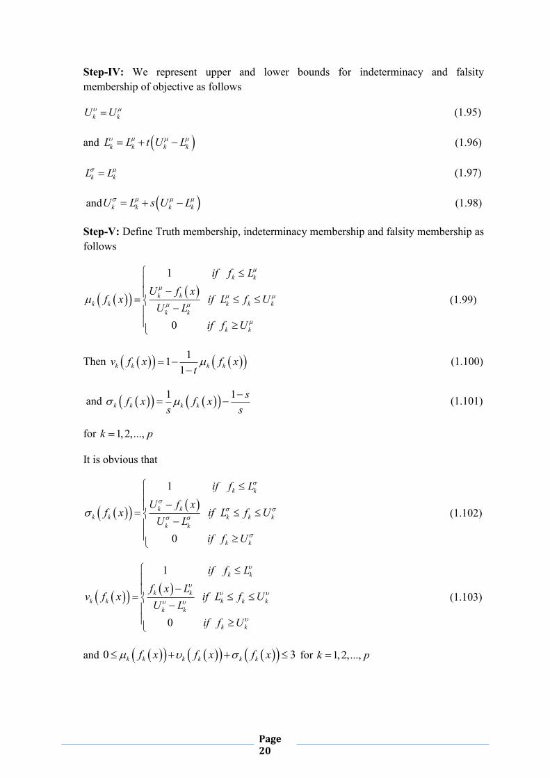
Step-IV: We represent upper and lower bounds for indeterminacy and falsity membership of objective as follows

k kU U (1.95)

and k k k kL L t U L

(1.96)

k kL L

(1.97)

and k k k kU L s U L

(1.98)

Step-V: Define Truth membership, indeterminacy membership and falsity membership as follows

1

0

k k

k kk k k k k

k k

k k

if f LU f x

f x if L f UU L

if f U

(1.99)

Then 11

1k k k kv f x f xt

(1.100)

and 1 1

k k k ksf x f x

s s

(1.101)

for

1,2,...,k p

It is obvious that

1

0

k k

k kk k k k k

k k

k k

if f LU f x

f x if L f UU L

if f U

(1.102)

1

0

k k

k kk k k k k

k k

k k

if f Lf x L

v f x if L f UU L

if f U

(1.103)

and 0 3k k k k k kf x f x f x for

1,2,...,k p

Page 21

Step-VI: Now a neutrosophic geometric programming technique for multi-objective non-linear programming problem with truth membership, falsity membership and indeterminacy membership function can be written as

(P1. 10)

1 1 2 2, ,....., p pMaximize f x f x f x

(1.104)

1 1 2 2, ,....., p pMinimize f x f x f x (1.105)

1 1 2 2, ,....., p pMaximize f x f x f x (1.106)

Such that

1 1

1i

itj

T na

i it jt j

f x C x

1,2,..,i m 1,2,..,j n (1.107)

0,jx

Where 0itC for all i and t. itja are real for all i,t,j

Using weighted sum method the multi-objective nonlinear programming problem (P1.10) reduces to

(P1. 11)

1

p

MA k k k k k k kk

Minimize V x w f x f x f x

(1.108)

1

1 1

1 1 1 1 11 11 1

kktj

T na

kt jp pt j k

MA k kk kk k k k

C xUMinimize V x w w

t s U L t s U L s

(1.109)

Such that

1 1

1i

itj

T na

i it jt j

f x C x

1,2,..,i m 1,2,..,j n (1.110)

0,jx


Excluding the constant term, the problem (P1.11) reduces to the following geometric programming problem

Page 22

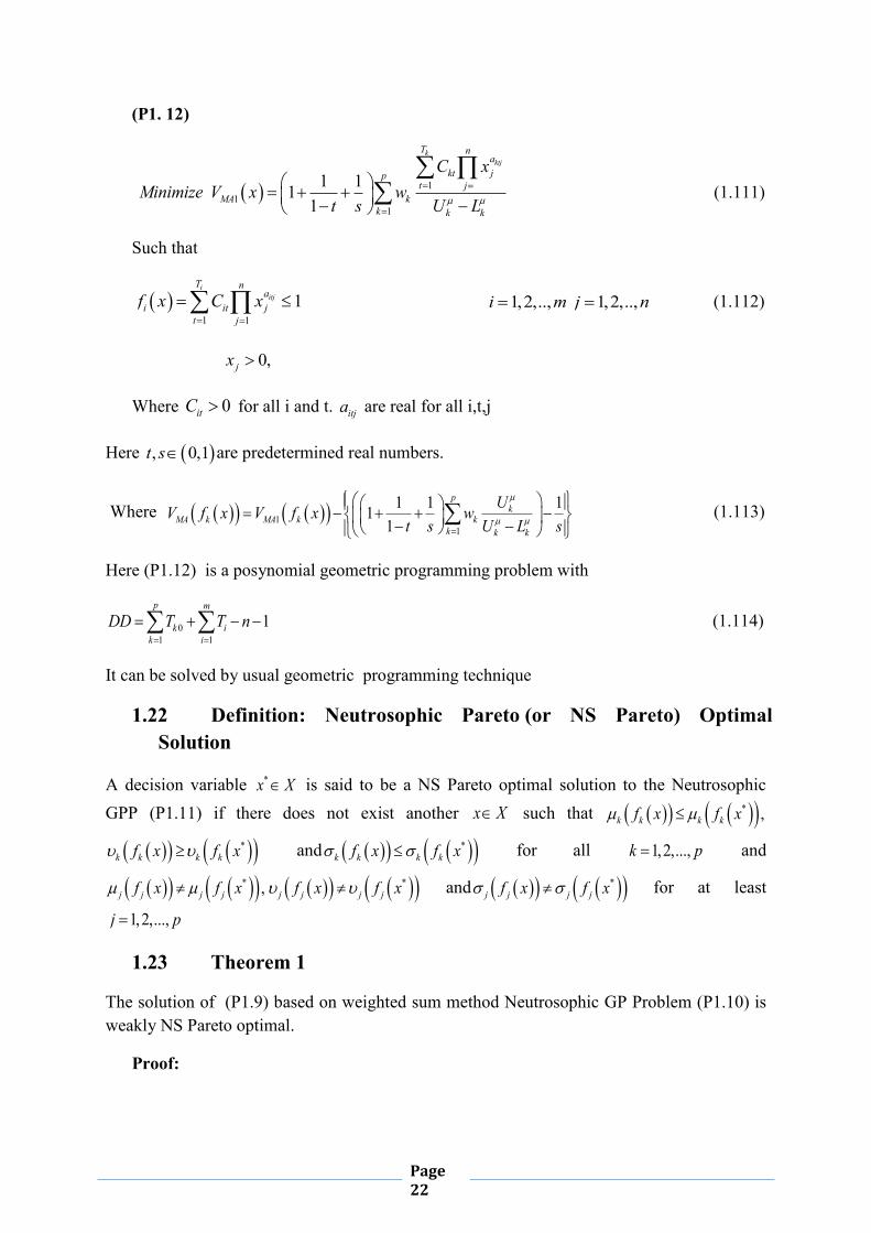
(P1. 12)

11

1

1 111

kktj

T na

kt jpt j

MA kk k k

C xMinimize V x w

t s U L

(1.111)

Such that

1 1

1i

itj

T na

i it jt j

f x C x

1,2,..,i m 1,2,..,j n (1.112)

0,jx


Here , 0,1t s are predetermined real numbers.

Where 11

1 1 111

pk

MA k MA k kk k k

UV f x V f x wt s U L s

(1.113)

Here (P1.12) is a posynomial geometric programming problem with

01 1

1p m

k ik i

DD T T n

(1.114)

It can be solved by usual geometric programming technique

1.22 Definition: Neutrosophic Pareto (or NS Pareto) Optimal Solution

A decision variable *x X is said to be a NS Pareto optimal solution to the Neutrosophic GPP (P1.11) if there does not exist another x X such that * ,k k k kf x f x

*k k k kf x f x and *

k k k kf x f x for all 1,2,...,k p and

* ,j j j jf x f x *j j j jf x f x and *

j j j jf x f x for at least

1,2,...,j p

1.23 Theorem 1

The solution of (P1.9) based on weighted sum method Neutrosophic GP Problem (P1.10) is weakly NS Pareto optimal.

Proof:

Page 23

Let *x X be the solution of Neutrosophic GP Problem.Let us suppose that it is not weakly M-N pareto optimal.In this case there exist another x X such that * ,k k k kf x f x


k k k kf x f x for all 1,2,...,k p .Observe that k kf x is

strictly monotone decreasing function with respect to kf x .This implies

*k k k kf x f x and k kf x is monotone increasing function with respect to ,kf x .

This implies *k k k kf x f x and k kf x is strictly monotone decreasing function

with respect to ,kf x so *k k k kf x f x .Thus we have

*

1 1,

p p

k k k k k kk k

w f x w f x

*

1 1

p p

k k k k k kk k

w f x w f x

and

*

1 1

p p

k k k k k kk k

w f x w f x

.This is a contradiction to the assumption that *x is a

solution of Neutrosophic GP Problem (P1.9).Thus *x is a weakly NS Pareto Optimal.

1.24 Theorem 2

The unique solution of Neutrosophic GP Problem (P1.10) based on weighted sum method is weakly NS Pareto optimal.

Proof:

Let *x X be the solution of Neutrosophic GP Problem.Let us suppose that it is not weakly NS pareto optimal. In this case there exist another x X such that * ,k k k kf x f x


k k k kf x f x for all 1,2,...,k p

and * ,l l l lf x f x *l l l lf x f x for at least one .l Observe that k kf x is

strictly monotone decreasing function with respect to ,kf x this implies

*k k k kf x f x and k kf x is monotone increasing function with respect to ,kf x .

This implies *k k k kf x f x and k kf x is strictly monotone decreasing function

with respect to ,kf x this implies *k k k kf x f x . Thus we have

*

1 1,

p p

k k k k k kk k

w f x w f x

*

1 1

p p

k k k k k kk k

w f x w f x

and

*

1 1

p p

k k k k k kk k

w f x w f x

. On the other hand uniqueness of *x means that

*

1 1,

p p

k k k k k kk k

w f x w f x

*

1 1

p p

k k k k k kk k

w f x w f x

and

Page 24

*

1 1

p p

k k k k k kk k

w f x w f x

. The two sets inequalities above are contradictory and thus

*x is weakly pareto optimal.

1.25 Illustrated Numerical Example

A multi-objective nonlinear programming problem can be written as

(P1. 13)

1 21 1 2 1 2,Minimize f x x x x

(1.115)

2 32 1 2 1 2, 2Minimize f x x x x

(1.116)

Such that 1 2 1x x

(1.117)

Here the pay-off matrix is

1 1 2 1 1 2

1

2

, ,

6.75 60.786.94 57.87

f x x f x x

xx

The truth membership,falsity membership and indeterminacy membership can be defined as follows

1 21 2

1 21 21 2

1 1 1 2

1 21 2

1 6.756.94 6.75 6.94

0.190 6.94

if x xx xf x if x x

if x x

(1.118)

2 31 2

2 32 31 2

2 2 1 2

2 31 2

1 2 57.8760.78 2 57.87 2 60.78

2.910 2 60.78

if x xx xf x if x x

if x x

(1.119)

1 1 1 111 ,

1v f x f x

t

(1.120)

2 2 2 111

1v f x f x

t

(1.121)

and 1 1 1 11 1 ,sf x f xs s

(1.122)

Page 25

2 2 2 21 1 sf x f xs s

(1.123)

Table 1.1 Optimal values of primal, dual variables and objective functions from Neutrosophic Geometric Programming Problem for different weights

Weights 1,w 2w

Optimal Dual Variables

*01,w *

02 ,w *11,w

*12 ,w

Optimal Primal Variables

*1 ,x *

2 ,x

Optimal Objectives

* * *1 1 2, ,f x x

* * *2 1 2,f x x

Sum of the Optimal Objectives

* * * * * *1 1 2 2 1 2, ,f x x f x x

0.5,0.5

0.6491609 0.3508391 1.3508391

2.3508391

0.3649261 0.6491609

6.794329

58.53371

65.32803

0.9,0.1

0.9415706 0.0584294 1.0584294

2.0584294

0.3395821

0.6604179

6.751768

60.21212

66.96388

0.1,0.9

0.1745920 0.8254080 1.8254080

2.8254080

0.3924920

0.6075080

6.903434

57.90451

64.80794

Table 1.2 Comparison of optimal solutions by IFGP and NSGP technique

Optimization Techniques


*1 ,x *

2 ,x

Optimal Objectives

* * *1 1 2, ,f x x

* * *2 1 2,f x x


* * * * * *1 1 2 2 1 2, ,f x x f x x

Intuitionistic Fuzzy Geometric Programming (IFGP)

0.36611 0.63389

6.797678

58.58212

65.37980

Proposed Neutrosophic Geometric Programming Technique

0.3649261

0.6491609

6.794329

58.53371

65.32803

Page 26

In Table 1.2,It has been seen that NSGP technique gives better optimal result than IFGP technique

1.26 Application of Neutrosophic Optimization in Gravel Box Design Problem

Gravel Box Problem: A total of 800 cubic meters of gravel is to be ferried across a river on a barrage. A box (with an open top) is to be built for this purpose.After the entire gravel has been ferried, the box is to be discarded.The transport cost of round trip of barrage of box is Rs 1 and the cost of materials of other two sides and bottom are Rs 10/m2.Find the dimension of the gravel box that is to be built for this purpose and the total optimal cost.Let length width and height of the box be 1 2 3, ,x m x m x m respectively. The area of the end of the gravel box is

22 3x x m . The area of the sides and bottom of the gravel box are 2

1 3x x m and 21 2x x m

respectively. The volume of the gravel box is 31 2 3 .x x x m Transport cost is Rs

1 2 3

80x x x

.Material

cost is 2 340x x .

So the gravel box problem can be formulated as multi-objective geometric programming problem as

(P1. 14)

1 1 2 3 2 31 2 3

80, , 40Minimize f x x x x xx x x

(1.124)

2 1 2 31 2 3

80, ,Minimize f x x xx x x

(1.125)

Such that 1 2 1 32 4x x x x

(1.126)

1 2 3, , 0x x x

Solution: Here pay off matrix is

1 2

1

2

95.24 63.78120 40

f x f x

xx

Table 1.3 Comparison of optimal solutions of gravel box problem between IFGP and NSGP Method

Optimization Techniques


*1 ,x *

2 ,x *3 ,x

Optimal Objectives

* * *1 1 2, ,f x x


* * * * * *1 1 2 2 1 2, ,f x x f x x

Page 27

* * *2 1 2,f x x

Intuitionistic Fuzzy Geometric Programming (IFGP)

1.2513842 1.5982302 0.7991151

101.1421624

50.0553670

151.1975294

Proposed Neutrosophic Geometric Programming Technique

1.2513843 1.59823000.7991150

101.1421582

50.0553655

151.1975237

1.27 Multi-Objective Neutrosophic Linear Programming Problem (MOLPP)

A general multi-objective linear programming problem with p objectives ,q constraints and n decision variables may be taken in the following form

(P1. 15)

1 1Maximize f X C X

(1.127)

2 2Maximize f X C X

(1.128)

.................................

..................................

p pMaximize f X C X

(1.129)

Subject to AX b (1.130)

0X (1.131)

Where 1 2, ,.......,i i i inC c c c for 1,2,..,i p (1.132)

,;ji q n

A a 1 2, ,....., ;nX x x x 1 2, ,.....,T

qb b b b for 1,2,.., ; 1,2,.....,j p i n (1.133)

Consider the multi-objective linear programming problem as

(P1. 16)

1 2, ,...., pMaximize f x f x f x (1.134)

Subject to

AX b (1.135)

Page 28

Where ,

,ij q nA a 1 2, ,....., ,T

nX x x x 1 2, ,....,T

qb b b b

(1.136)

Now the decision set nD , conjunction of neutrosophic objectives and constraints are defined

as 1 1

, , ,n n n

p qn n n

k j D D Dk j

D G C x T x I x F x

(1.137)

Here

1 2 1 2

, ,......, ; , ,.....,n n n n n n np qD G G G C C G

T x T x T x T x T x T x T x for all .x X (1.138)

1 2 1 2


I x I x I x I x I x I x I x for all .x X (1.139)

1 2 1 2


F x F x F x F x F x F x F x for all .x X (1.140)

Here , ,n n nD D DT x I x F x are Truth membership function, Indeterminacy membership

function, Falsity membership Functions of Neutrosophic Decision set respectively. Now

using the definition of Smarandache‟s intersection of neutrosophic sets and criteria of

decision making ,the optimum linear programming problem can be formulated as

Model-I-AL,BL

(P1. 17)

Max (1.141)

Min (1.142)

Max (1.143)

Such that

nkG

T x (1.144)

nkC

T x

(1.145)

nkG

I x

(1.146)

nkC

I x

(1.147)

nkG

T x

(1.148)

nkC

T x

(1.149)

Page 29

1,2,...,k p

3 (1.150)

; (1.151)

;

(1.152)

, , 0,1

(1.153)

In this algorithm we have considered the indeterminacy membership function as of

decreasing sense and increasing sense respectively in Model-I-AL and Model-BL

respectively

But in real world situation a decision maker needs to minimize indeterminacy or hesitancy

So using the another definition of Smarandache‟s intersection of neutrosophic sets and

criteria of decision making the optimum linear programming problem is formulated as

Model-II-AL,BL

(P1. 18)

Max (1.154)

Min (1.155)

Min (1.156)

Such that

nkG

T x (1.157)

nkC

T x

(1.158)

nkG

I x

(1.159)

nkC

I x

(1.160)

nkG

T x

(1.161)

nkC

T x

(1.162)

1,2,...,k p

3 (1.163)

; (1.164)

; (1.165)

Page 30

, , 0,1

(1.166)

In this algorithm we have considered the indeterminacy membership function as per

decreasing sense and increasing sense respectively in Model-II-AL and Model-II-BL.

Computational Algorithm 1 (Linear Membership Function)

Step-I: Pick the objective function and solve it as a single objective subjected to the

constraints. Continue the process k-times for k different objective functions. Find value of

objective functions and decision variables.

Step-II: To build membership functions, goals and tolerances should be determined at first.

Using ideal solutions, obtained in step-I we find the values of all the objective functions at

each ideal solution and construct pay-off matrix as follows

* 1 1 11 2

2 * 2 22 2 2

*1 2

........

........

........ ........ ........ .........

.......

p

p p pp

f x f x f x

f x f x f x

f x f x f x

Step-III: From step-II we find the upper and lower bounds of each objective functions

*maxTk k rU f x and *minT

k k rL f x where 1 r k for truth membership functions

of objectives.

Step-IV: We represent upper and lower bounds for indeterminacy and falsity membership of

objectives as follows for

Model-I,II-AL,AN

I Tk kL L and I T T T

k k k kU L U L

(1.167)

F T T Tk k k kL L t U L

(1.168)

F Tk kU U

for Model-I,II-BL,BN

F T Ik k kU U U


I T T Tk k k kL L U L

Here and t are two predominant real numbers in 0,1

Page 31

Step-V: Define Truth membership, Indeterminacy membership, Falsity membership

functions (For Model-I,II-AL,BL) as follows

1

0

Tk k

Tk k T T

k k k k kT Tk k

Tk k

if f x LU f x

T f x if L f x UU L

if f x U

(1.169)

For Model-I,II-AL

0

1

Ik k

Ik k I I

k k k k kI Ik k

Ik k

if f x LU f x

I f x if L f x UU L

if f x U

(1.170)

For Model-I,II-BL

0

1

Ik k

Ik k I I

k k k k kI Ik k

Ik k

if f x Lf x L

I f x if L f x UU L

if f x U

(1.171)

0

1

Fk k

Fk k F F

k k k k kF Fk k

Fk k

if f x Lf x L

F f x if L f x UU L

if f x U

(1.172)

Step-VI: Now neutrosophic optimization method for MOLP problem gives an equivalent

linear programming problem as Model-I-AL and Model-I-BL as

Model-I-AL,BL

(P1. 19)

Maximize (1.173)

k kT f x

(1.174)

k kI f x

(1.175)

k kF f x for 1,2,3,..,k p (1.176)

3, (1.177)

, (1.178)

Page 32

, (1.179)

, , 0,1

(1.180)

,Ax b (1.181)

0x (1.182)

Where ,

;ji q nA a 1 2, ,....., ;nX x x x 1 2, ,.....,

T

qb b b b for 1,2,.., ; 1,2,.....,j p i n

Where in case of Model-I-AL we have considered Indeterminacy membership function as of

decreasing sense and in Model-I-BL we have considered Indeterminacy membership function

as of inceasing sense.

Again Model-II-AL and Model-II-BL can be formulated as

Model-II-AL,BL

(P1. 20)

Maximize (1.183)

k kT f x

(1.184)

k kI f x

(1.185)

k kF f x for 1,2,3,..,k p (1.186)

3, (1.187)

, (1.188) , (1.189)

, , 0,1

(1.190)

,Ax b (1.191)

0x (1.192)

Where ,

;ji q nA a 1 2, ,....., ;nX x x x 1 2, ,.....,

T

qb b b b for 1,2,.., ; 1,2,.....,j p i n Here

Here Model-II-AL,and Model-II-BL stand for neutrosophic algorithm with decreasing

indeterminacy membership function and increasing indeterminacy membership function

respectively. The above problems can be reduced to equivalent linear programming

problem as

Model-I-AL

(P1. 21)

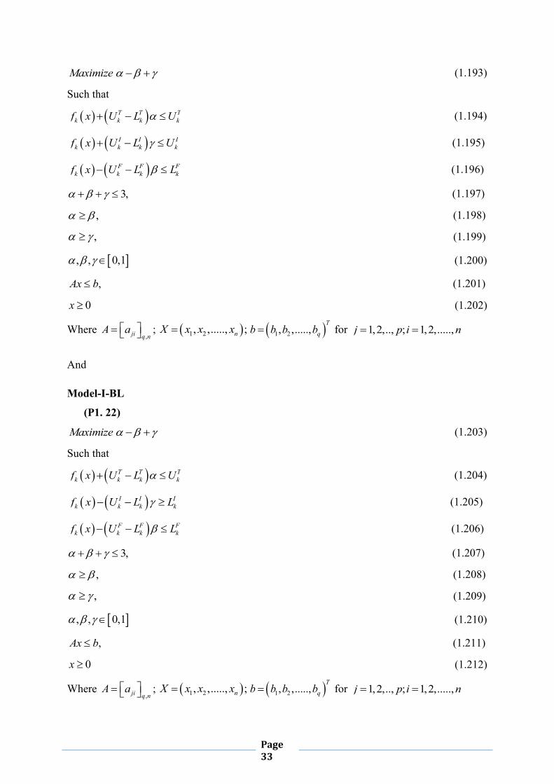
Page 33

Maximize (1.193)

Such that

T T Tk k k kf x U L U

(1.194)

I I Ik k k kf x U L U

(1.195)

F F Fk k k kf x U L L

(1.196)

3, (1.197)

, (1.198) , (1.199)

, , 0,1

(1.200)

,Ax b (1.201)

0x (1.202)

Where ,

;ji q nA a 1 2, ,....., ;nX x x x 1 2, ,.....,

T

qb b b b for 1,2,.., ; 1,2,.....,j p i n

And

Model-I-BL

(P1. 22)

Maximize (1.203)

Such that


(1.204)

I I Ik k k kf x U L L

(1.205)


(1.206)

3, (1.207)

, (1.208) , (1.209)

, , 0,1

(1.210)

,Ax b (1.211)

0x (1.212)

Where ,

;ji q nA a 1 2, ,....., ;nX x x x 1 2, ,.....,

T

qb b b b for 1,2,.., ; 1,2,.....,j p i n

Page 34

And

Model-II-AL

(P1. 23)

Maximize (1.213)

Such that


(1.214)


(1.215)


(1.216)

3, (1.217)

, (1.218) , (1.219)

, , 0,1

(1.220)

,Ax b (1.221)

0x (1.222)

Where ,

;ji q nA a 1 2, ,....., ;nX x x x 1 2, ,.....,

T

qb b b b for 1,2,.., ; 1,2,.....,j p i n

And

Model-II-BL

(P1. 24)

Maximize (1.223)

Such that


(1.224)

I I I

k k k kf x U L L

(1.225)


(1.226)

3, (1.227)

Page 35

, (1.228) , (1.229)

, , 0,1

(1.230)

,Ax b (1.231)

0x (1.232)

Where ,

;ji q nA a 1 2, ,....., ;nX x x x 1 2, ,.....,

T

qb b b b for 1,2,.., ; 1,2,.....,j p i n

And

Computational Algorithm 2 (Non Linear Membership Function)

Repeat step 1 to 4 as same as computational algorithm 1 and construct pay off matrix.

Step-V: Assumes that solutions so far computed by algorithm follow exponential function for

Truth membership, hyperbolic membership function for Falsity membership and exponential

function for Indeterminacy membership function (Model-I-AN,Model-I-BN) given as

0

1 exp

1

Tk k

Tk k T T

k k k k kT Tk k

Tk k

if f x L

U f xT f x if L f x U

U L

if f x U

(1.233)

For Model-I,II-AN as

0

exp

1

Ik k

Ik k I I

k k k k kI Ik k

Ik k

if f x L

U f xI f x if L f x U

U L

if f x U

(1.234)

For Model-I,II-BN as

0

exp

1

Ik k

Ik k I I

k k k k kI Ik k

Ik k

if f x L

f x LI f x if L f x U

U L

if f x U

(1.235)

Page 36

0

1 1 tanh2 2 2

1

Fk k

F FF Fk k

k k k k k k k

Fk k

if f x L

U LF f x f x if L f x U

if f x U

(1.236)

Step-VI: Now neutrosophic optimization method for MOLP problem with exponential Truth

membership, Hyperbolic falsity membership and exponential indeterminacy membership

functions give the equivalent linear programming problem as

Model-I-AN,

(P1. 25)

Maximize (1.237)

Such that

4

T Tk k T

k k

U Lf x U

(1.238)


(1.239)

2

F Fk k

kk

U Lf x

(1.240)

3, (1.241)

, (1.242)

, (1.243)

, , 0,1

(1.244)

,Ax b (1.245)

0x (1.246)

Where ,

;ji q nA a 1 2, ,....., ;nX x x x 1 2, ,.....,

T

qb b b b for 1,2,.., ; 1,2,.....,j p i n

log 1 ,

(1.247)

log ,

(1.248)

1tanh 2 1 ,

(1.249)

4,

(1.250)

Page 37

6k F F

k kU L

(1.251)

And

Model-I-BN

(P1. 26)

Maximize (1.252)

Such that

4

T Tk k T

k k

U Lf x U

(1.253)


(1.254)

2

F Fk k

kk

U Lf x

(1.255)

3, (1.256)

, (1.257)

, (1.258)

, , 0,1

(1.259)

,Ax b (1.260)

0x (1.261)

Where ,

;ji q nA a 1 2, ,....., ;nX x x x 1 2, ,.....,

T

qb b b b for 1,2,.., ; 1,2,.....,j p i n

log 1 ,

(1.262)

log ,

(1.263)

1tanh 2 1 ,

(1.264)

4,

(1.265)

6k F F

k kU L

(1.266)

Model-II-AN,

(P1. 27)

Page 38

Maximize (1.267)

Such that

4

T Tk k T

k k

U Lf x U

(1.268)


(1.269)

2

F Fk k

kk

U Lf x

(1.270)

3, (1.271)

, (1.272)

, (1.273)

, , 0,1

(1.274)

,Ax b (1.275)

0x (1.276)

Where ,

;ji q nA a 1 2, ,....., ;nX x x x 1 2, ,.....,

T

qb b b b for 1,2,.., ; 1,2,.....,j p i n

log 1 ,

(1.277)

log ,

(1.278)

1tanh 2 1 ,

(1.279)

4,

(1.280)

6k F F

k kU L

(1.281)

Model-II-BN,

(P1. 28)

Maximize (1.282)

Such that

4

T Tk k T

k k

U Lf x U

(1.283)


(1.284)

Page 39

2

F Fk k

kk

U Lf x

(1.285)

3, (1.286)

, (1.287)

, (1.288)

, , 0,1

(1.289)

,Ax b (1.290)

0x (1.291)

Where ,

;ji q nA a 1 2, ,....., ;nX x x x 1 2, ,.....,

T

qb b b b for 1,2,.., ; 1,2,.....,j p i n

log 1 ,

(1.292)

log ,

(1.293)

1tanh 2 1 ,

(1.294)

4,

(1.295)

6k F F

k kU L

(1.296)

The above crisp linear programming problems can be solved by LINGO Tool Box.

1.28 Production Planning Problem

Consider a park of six machine types whose capacities are to be devoted to production of

three products. A current capacity portfolio is available, measured in machine hours for each

machine capacity unit price according to machine type. Necessary data are summarized

below in table 1.4.

Table 1.4 Physical Parameter values

Machine Type Machine hours Unit price

($ 100 per hour)

Products

1x 2x 3x

Milling Machine 1400 0.75 12 17 0

Page 40

Lathe 1000 0.60 3 9 8

Grinder 1750 0.35 10 13 15

Jig Saw 1325 0.50 6 0 16

Drill Press 900 0.15 0 12 7

Band Saw 1075 0.65 9.5 9.5 4

Total capacity cost $ 4658.75

Let 1 2 3, ,x x x denote three products, then the complete mathematical formulation of the above

mentioned problem as Multi-objective linear programming problem can be given as

(P1. 29)

1 1 2 350 100 17.5Maximize f x x x x (profit) (1.297)

2 1 2 392 75 50Maximize f x x x x (quality) (1.298)

3 1 2 325 100 75Maximize f x x x x (worker satisfaction) (1.299)

Subject to

1 212 17 1400;x x

(1.300)

1 2 33 9 8 1400;x x x

(1.301)

1 2 310 13 15 1750x x x

(1.302)

1 36 16 1325x x

(1.303)

1 2 3, , 0x x x

(1.304)

Table 1.5 Positive Ideal Solution

1f 2f 3f

1Max f 8041.14 10020.33 9319.25

2Max f 5452.63 10950.59 5903.00

3Max f 7983.60 10056.99 9355.90

Page 41

Table 1.6 Comparison of optimal solutions by IFO and NSO Technique

Optimization

Technique

Optimal

Decision

Variable * * *1 2 3, ,x x x

Optimal

Objective

Function * * *

1 2 3, ,f f f

Sum of

optimal

objective

values

Intuitionistic Fuzzy

Optimization(IFO)

*1 62.82;x *2 38.005;x *3 41.84x

*1 7673.2;f *

2 10721.81;f *

3 8508.5f

26903.51

Proposed

Neutrosophic

Optimization(NSO)

1 1, 1294.255

2 2, 465.13

3 3, 1726.450

Model-I-AL

*1 79.99;x *2 7.073;x

*3 42.611x

*1 5452.630;f

*2 10020.33;f

*3 5903.0f

12375.96

Model-I-BL *1 68.89;x *2 25.09;x *3 45.30x

*1 6746.855;f

*2 465.13;f *

3 7629.45f

14841.435

Model-II-AL *1 68.89;x *2 25.09;x *3 45.30x

*1 6746.855;f

*2 465.13;f *

3 7629.45f

14841.435

Model-II-BL *1 79.99;x *2 7.07;x *3 42.62x

*1 5452.63;f *

2 10020.33;f *

3 5903.0f

21375.96

Model-I-AN *1 66.58;x

*2 22.05;x *3 43.95x

*1 6303.59;f

*2 9977.03;f *

3 7166.53f

23447.15

Model-I-BN *1 64.088;x

*2 30.74;x *3 46.422x

*1 7090.533;f

*2 10522.56;f *

3 8157.639f

25770.732

Page 42

Model-II-AN *1 64.088;x

*2 30.74;x

*3 46.42x

*1 7090.533;f

*2 10522.56;f

*3 8157.639f

25770.732

Model-II-BN *1 66.58;x *2 22.06;x

*3 43.96x

*1 6303.89;f *

2 9977.61;f

*3 7167.44f

23448.94

Table 1.6 shows that neutrosophic optimization gives better result than intuitioistic fuzzy

optimization.

1.29 Neutrosophic Optimization (NSO)Technique to solve Single-

Objective Minimization Type Nonlinear Programming

(SONLP) Problem

Let us consider a SONLP problem as

(P1. 30)

Minimize f x (1.305)

1,2,...,j jg x b j m (1.306)

0x (1.307)

Usually constraint goals are considered as fixed quantity .But in real life problem,the

constraint goal cannot be always exact. So we can consider the constraint goal for less than

type constraints at least jb and it may possible to extend to 0j jb b .This fact seems to take the

constraint goal as a NS and which will be more realistic descriptions than others. Then the

NLP becomes NSO problem with neutrosophic resources, which can be described as follows

(P1. 31)


1,2,....,nj jg x b j m (1.309)

0x (1.310)

To solve the NSO (P1.31), following Werner‟s [118] and Angelov [3] we are presenting a

solution procedure for SONSO problem (P1.31) as follows

Step-1: Following Werner‟s approach solve the single objective non-linear programming

problem without tolerance in constraints (i.e j jg x b ),with tolerance of acceptance in

constraints (i.e 0j j jg x b b ) by appropriate non-linear programming technique

Page 43

Here they are

(P1. 32)

Sub-problem-1


1,2,....,j jg x b j m

(1.312)

0x (1.313)

(P1. 33)

Sub-problem-2


0 , 1,2,....,j j jg x b b j m (1.315)

0x (1.316)

we may get optimal solutions * 1 * 1,x x f x f x and * 2 * 2,x x f x f x for sub-problem

1 and 2 respectively.

Step-2: From the result of step 1 we now find the lower bound and upper bound of objective

functions [Fig.-1.1]. If , ,T I Ff x f x f xU U U be the upper bounds of truth, indeterminacy , falsity

function for the objective respectively and , ,T I Ff x f x f xL L L be the lower bound of truth,

indeterminacy, falsity membership functions of objective respectively then

1 2max , ,Tf xU f x f x (1.317)

1 2min , ,Tf xL f x f x

(1.318)

for Model-I,II-AL,AN

I T I T T Tf x f x f x f x f x f xL L and U L s U L (1.319)

;F T F T T Tf x f x f x f x f x f xU U and L L t U L (1.320)


F T Ik k kU U U

F T T Tk k k kL L s U L

I T T Tk k k kL L t U L

Here ,t s are predetermined real numbers in 0,1

Page 44

Fig.-1.1 Rough Sketch of Lower and Upper bounds of Truth, Indeterminacy and Falsity

Membership Functions of Objective of (P1.31)

The initial neutrosophic model (Model -I)with aspiration levels of objectives can be

formulated as

(P1. 34)

Find x

(1.321)

So as to satisfy

n T

f xf x L with tolerance T T

f x f xU L for degree of truth membership (1.322)

n I

f xf x L with tolerance I I

f x f xU L for degree of indeterminacy membership (1.323)

n F

f xf x U with tolerance F F

f x f xU L for degree of falsity membership (1.324)

nj jg x b with tolerance 0

jb for degree of truth membership (1.325)

nj jg x b with tolerance

jg x for degree of indeterminacy membership (1.326)

0nj j jg x b b with tolerance 0

jj j j g xb b b for degree of falsity membership

(1.327)

for 1,2,...j m , ; 0,1

j j j

T Tg x g x g xt U L t and

; 0,1j j j

T Tg x g x g xs U L s

and for Mode-II it can be formulated as

(P1. 35)

Find x

(1.328)

So as to satisfy

n T

f xf x L with tolerance T T

f x f xU L for degree of truth membership (1.329)

Page 45

n I

f xf x U with tolerance I I

f x f xU L for degree of indeterminacy membership (1.330)

n F

f xf x U with tolerance F F

f x f xU L for degree of falsity membership (1.331)

nj jg x b with tolerance 0

jb for degree of truth membership (1.332)

j

nj j g xg x b with tolerance

jg x for degree of indeterminacy membership (1.333)

0nj j jg x b b with tolerance 0

jj j j g xb b b for degree of falsity membership

(1.334) For 1,2,...j m ,

; 0,1j j j

T Tg x g x g xt U L t

(1.335)

and ; 0,1

j j j

T Tg x g x g xs U L s

(1.336)

Here ' 'n denotes inequality in neutrosophic sense.

Step-3: In this step we calculate linear membership for truth, indeterminacy and falsity

membership functions of objective as follows

1

0

Tf x

Tf x T T

f x f x f xT Tf x f x

Tf x

if f x L


U L

if f x U

(1.337)

For Model-I,II-AL

1

0

If x

If x I I

f x f x f xI If x f x

If x

if f x L


U L

if f x U

(1.338)

For Model-I,II-BL

1

0

If x

If x I I


If x

if f x U


U L

if f x L

(1.339)

Page 46

0

1

Ff x

Ff x F F

f x f x f xF Ff x f x

Ff x

if f x L

f x LF f x if L f x U

U L

if f x U

(1.340)

and exponential and hyperbolic membership for truth, indeterminacy and falsity membership

functions as follows

1

1 exp

0

Tf x

Tf x T T

f x f x f xT Tf x f x

Tf x

if f x L


U L

if f x U

(1.341)

For Model-I,II-AN

1

exp

0

If x

If x I I


If x

if f x L


U L

if f x U

(1.342)

For Model-I,II-BN

1

exp

0

If x

If x I I


If x

if f x U


U L

if f x L

(1.343)

0

1 1 tanh2 2 2

1

Ff x

F Ff x f x F F

f x f x f x f x

Ff x

if f x L


if f x U

(1.344)

Step-4: In this step using linear, exponential and hyperbolic function for truth,

indeterminacy and falsity membership functions, we may calculate membership function for

constraints as follows

Page 47

00

0

0

1

0

j

j j

j j jj j j j jg x

j

j j

if g x b

b b g xT g x if b g x b b

b

if g x b

(1.345)

For Model-I,II-AL

1

0

j

j j

j

j

j j

j jg xj j j jg x g x

g x

j j g x

if g x b

b g xI g x if b g x b

if g x b

(1.346)

For Model-I,II-BL

0

00

1

0

j

j j

j

j

j j j

j j g xj j j j jg x g x

j g x

j j g x

if g x b b

g x bI g x if b g x b b

b

if g x b

(1.347)

00

0

0

1

j

j

j j

j

j j g x


j g x

j j j

if g x b

g x bF g x if b g x b b

b

if g x b b

(1.348)

where for

01,2,..., 0 ,j j jg x g xj m b . and

0

0

1

1 exp

0

j

j

j j

j j

Tjg x

j j j j jg x T Tg x g x

j j j

if g x b

U g xT g x if b g x b b

U L

if g x b b

(1.349)

For Model-I,II-AN

1

exp

0

j

j j

j

j

j j

j jg x

j j j jg x g xg x

j j g x

if g x b

b g xI g x if b g x b

if g x b

(1.350)

Page 48

For Model-I,II-BN

0

0

0

1

exp

0

j

j j

j

j

j j j

j j g x

j j j j jg x g x

j g x

j j g x

if g x b b

g x bI g x if b g x b b

b

if g x b

(1.351)

00

0

0

21 1 tanh2 2 2

1

j

j

j j j

j j g x

j j g xj j j j j jg x g x g x

j j j

if g x b

b bF g x g x if b g x b b

if g x b b

(1.352)

where , are non-zero parameters prescribed by the decision maker and for

01,2,....., 0 ,

j j jg x g xj m b .

Step-5: Now using NSO for single objective optimization technique the optimization

problem (P1.34) and (P1.35)can be formulated as

(P1. 36)

Model-I-AN,BN

Maximize

(1.353)

Such that

;f xT x

(1.354)

;jgT x

(1.355)

;f xI x (1.356)

;jgI x

(1.357)

;f xF x

(1.358)

;jgF x

(1.359)

3; (1.360)

; ; (1.361)

, , 0,1 (1.362)

Page 49

In case of Model-I-AN and Model-I-BN we will consider indeterminacy membership

function in decreasing sense and increasing sense respectively.

(P1. 37)

Model-II-AN,BN

Maximize

(1.363)

Subject to

;f xT x

(1.364)

;jgT x

(1.365)

;f xI x (1.366)

;jgI x

(1.367)

;f xF x

(1.368)

;jgF x

(1.369)

3; (1.370)

; ; (1.371)

, , 0,1 (1.372)

In case of Model-II-A and Model-II-B we will consider indeterminacy membership function

in decreasing sense and increasing sense respectively.

Now the above problem (Model-I) (P1.36) can be simplified to following crisp linear

programming problem for linear membership function as

Model-I-AL

(P1. 38)

Maximize (1.373)

. ;T T Tf x f x f xsuch that f x U L U

(1.374)

. ;I I If x f x f xf x U L U

(1.375)

. ; 1,2,....,F F Ff x f x f xf x U L L for k p

(1.376)

3; (1.377)

; (1.378)

Page 50

; (1.379)

, , 0,1 ; (1.380)

,j jg x b (1.381)

0,x (1.382)

Model-I-BL

(P1. 39)

Maximize (1.383)


(1.384)

. ;I I If x f x f xf x U L L

(1.385)


(1.386)

3; (1.387)

; (1.388)

; (1.389)

, , 0,1 ; (1.390)

,j jg x b (1.391)

0,x (1.392)

and for nonlinear membership function as

Model-I-AN

(P1. 40)

Maximize (1.393)

Such that

;

T Tf x f x T

f x

U Lf x U

(1.394)

;T

f x f x f xf x L

(1.395)

;2

T Tf x f x f x

f x

U Lf x

(1.396)

Page 51

0

0;jj j j

bg x b b

(1.397)

0 ;

j jj jg x g xg x b

(1.398)

02

;2

jj j g xj

g x

b bg x

(1.399)

3; (1.400)

; (1.401)

; (1.402)

, , 0,1

(1.403)

Where

ln 1 ;

(1.404)

4; (1.405)

6 ;f x F F

f x f xU L

(1.406)

0

6 , 1,2,...,jg x

j j

for j mb

(1.407)

ln ; (1.408)

1tanh 2 1 .

(1.409)

Model-I-BN

(P1. 41)

Maximize (1.410)

Such that

;

T Tf x f x T

f x

U Lf x U

(1.411)

;T T T

f x f x f x f x f xf x U L L

(1.412)

;2

T Tf x f x f x

f x

U Lf x

(1.413)

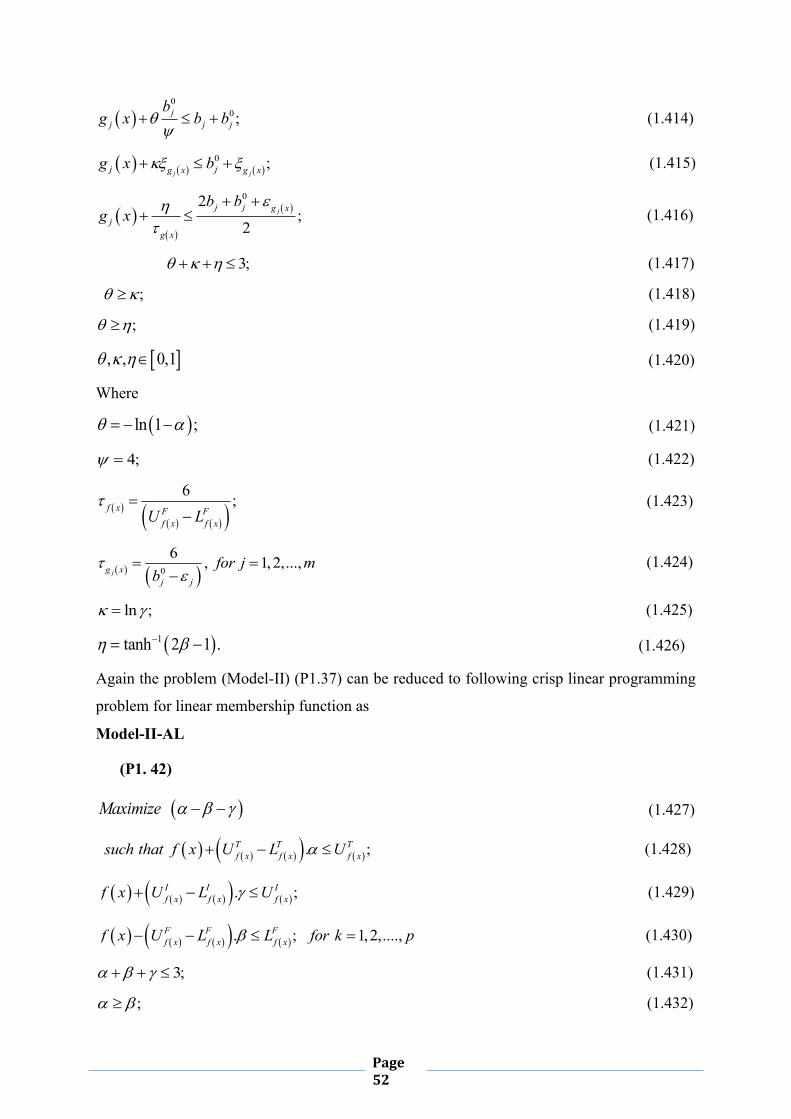
Page 52

0

0;jj j j

bg x b b

(1.414)

0 ;

j jj jg x g xg x b

(1.415)

02

;2

jj j g xj

g x

b bg x

(1.416)

3; (1.417)

; (1.418)

; (1.419)

, , 0,1

(1.420)

Where

ln 1 ;

(1.421)

4; (1.422)

6 ;f x F F

f x f xU L

(1.423)

0

6 , 1,2,...,jg x

j j

for j mb

(1.424)

ln ; (1.425)

1tanh 2 1 .

(1.426)

Again the problem (Model-II) (P1.37) can be reduced to following crisp linear programming

problem for linear membership function as

Model-II-AL

(P1. 42)

Maximize (1.427)


(1.428)

. ;I I If x f x f xf x U L U

(1.429)


(1.430)

3; (1.431)

; (1.432)

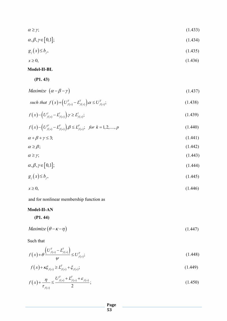
Page 53

; (1.433)

, , 0,1 ; (1.434)

,j jg x b (1.435)

0,x (1.436)

Model-II-BL

(P1. 43)

Maximize (1.437)


(1.438)

. ;I I If x f x f xf x U L L

(1.439)


(1.440)

3; (1.441)

; (1.442)

; (1.443)

, , 0,1 ; (1.444)

,j jg x b (1.445)

0,x (1.446)

and for nonlinear membership function as

Model-II-AN

(P1. 44)

Maximize (1.447)

Such that

;

T Tf x f x T

f x

U Lf x U

(1.448)

;T

f x f x f xf x L

(1.449)

;2

T Tf x f x f x

f x

U Lf x

(1.450)

Page 54

0

0;jj j j

bg x b b

(1.451)

0 ;

j jj jg x g xg x b

(1.452)

02

;2

jj j g xj

g x

b bg x

(1.453)

3; (1.454)

; (1.455)

; (1.456)

, , 0,1

(1.457)

Where

ln 1 ;

(1.458)

4; (1.459)

6 ;f x F F

f x f xU L

(1.460)

0

6 , 1,2,...,jg x

j j

for j mb

(1.461)

ln ; (1.462)

1tanh 2 1 .

(1.463)

Model-II-BN

(P1. 45)

Maximize (1.464)

Such that

;

T Tf x f x T

f x

U Lf x U

(1.465)

;T T T

f x f x f x f x f xf x U L L

(1.466)

;2

T Tf x f x f x

f x

U Lf x

(1.467)

Page 55

0

0;jj j j

bg x b b

(1.468)

0 ;

j jj jg x g xg x b

(1.469)

02

;2

jj j g xj

g x

b bg x

(1.470)

3; (1.471)

; (1.472)

; (1.473)

, , 0,1

(1.474)

Where

ln 1 ;

(1.475)

4; (1.476)

6 ;f x F F

f x f xU L

(1.477)

0

6 , 1,2,...,jg x

j j

for j mb

(1.478)

ln ; (1.479)

1tanh 2 1 .

(1.480)

All these crisp nonlinear programming problems (P1.38-P1.45) can be solved by appropriate

mathematical algorithm.

1.30 Neutrosophic Optimization Technique to solve Minimization Type Multi-Objective Non-linear Programming Problem for Linear Membership Function

A non-linear multi-objective optimization problem is of the form

(P1. 46)

1 2, ,..., pMinimize f x f x f x (1.481)

,j jg x b 1,2,...,j q (1.482)

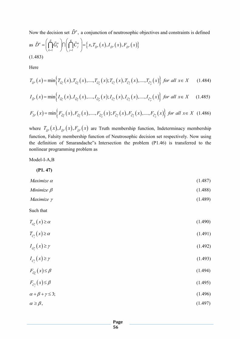
Page 56

Now the decision set ,nD a conjunction of neutrosophic objectives and constraints is defined

as 1 1

, , ,n n n

p qn n n

k j D D Dk j

D G C x T x I x F x

(1.483)

Here

1 2 1 2

min , ,...., ; , ,....,n n n n n n np pD G G G C C C

T x T x T x T x T x T x T x for all x X (1.484)

1 2 1 2


I x I x I x I x I x I x I x for all x X (1.485)

1 2 1 2


F x F x F x F x F x F x F x for all x X (1.486)

where , ,n n nD D DT x I x F x are Truth membership function, Indeterminacy membership

function, Falsity membership function of Neutrosophic decision set respectively. Now using the definition of Smarandache‟s Intersection the problem (P1.46) is transferred to the nonlinear programming problem as

Model-I-A,B

(P1. 47)

Maximize (1.487)

Minimize (1.488)

Maximize (1.489)

Such that

nkG

T x (1.490)

njC

T x (1.491)

njG

I x (1.492)

njC

I x (1.493)

nkG

F x (1.494)

njC

F x (1.495)

3; (1.496)

, (1.497)

Page 57

(1.498)

, , 0,1 (1.499)

In Model-I-A we will consider indeterminacy function as decreasing sense and in Model-I-B we will consider indeterminacy membership function as increasing sense.

Again in real world practical problem a decision maker needs to minimize hesitancy function.So the nonlinear programming problem can be formulated as

Model-II-A,B

(P1. 48)

Maximize (1.500)

Minimize (1.501)

Minimize (1.502)

Such that

nkG

T x (1.503)

njC

T x (1.504)

njG

I x (1.505)

njC

I x (1.506)

nkG

F x (1.507)

njC

F x (1.508)

3; (1.509)

, (1.510)

(1.511)

, , 0,1

In Model-II-A we will consider indeterminacy function as decreasing sense and in Model-II-B we will consider indeterminacy membership function as increasing sense.

Now this non-linear programming problem (P1.47,P1.48) can be easily solved by appropriate mathematical algorithm to give solution of multi-objective linear programming problem (P1.46) by neutrosophic optimization approach.

Page 58

Step-1 Solve the MONLP(P1.46) as a single objective non-linear problem p times for each problem by taking one of the objectives at a time and ignoring the others. These solution are known as ideal solutions. Let kx be the respective optimal solution for the k th different objective and evaluate each objective values for all these k th optimal solution.

Step-2 From the result of Step-1,determine the corresponding values for every objective for each derived solution .With the values of all objectives at each ideal solutions, pay-off matrix can be formulated as follows

* 1 1 11 2

2 * 2 21 2

*1 2

....

....

... ... .... ...

....

p

p

p p pp

f x f x f x

f x f x f x

f x f x f x

Step-3 For each objective kf x ,the lower bound TkL and upper bound T

kU as

*maxT rk kU f x (1.512)

and *minT rk kL f x (1.513)

where 1,2,...,r k for truth membership function of objectives.

Step-4 We represents upper and lower bounds for indeterminacy and falsity membership of objectives as follows

Model- I,II-AL,AN

F Tk kU U and

F T T Tk k k kL L t U L (1.514)

I Tk kU U and

I T T Tk k k kL L s U L (1.515)

Here t and s are predetermined real number in 0,1

Model-I,II-BL,BN

F T Ik k kU U U and



Page 59

I T T Tk k k kL L s U L

Here t and s are predetermined real number in 0,1

Step-5 Define Truth membership, Indeterminacy membership, Falsity membership functions as follows

1

0

Tk k

Tk k T T

k k k k kT Tk k

Tk k

if f x LU f x

T f x if L f x UU L

if f x U

(1.516)

For Model-I,II-AL

1

0

Ik k

Ik k I I

k k k k kI Ik k

Ik k

if f x LU f x

I f x if L f x UU L

if f x U

(1.517)

For Model-I,II-BL

1

0

Ik k

Ik k I I

k k k k kI Ik k

Ik k

if f x Uf x L

I f x if L f x UU L

if f x L

(1.518)

1

0

Fk k

Fk k F F

k k k k kF Fk k

Fk k

if f x Lf x L

F f x if L f x UU L

if f x U

(1.519)

Step-6 Now neutrosophic optimization method for MONLP problem gives an equivalent nonlinear-programing problem as

Model-I-A,B

(P1. 49)

Max

(1.520)

Such that

Page 60

;k kT f x (1.521)

;k kI f x

(1.522)

;k kF f x

(1.523)

3;

(1.524)

;

(1.525)

;

(1.526)

, , 0,1 ;

(1.527)

; 0j jg x b x

(1.528)

1,2,.., ; 1,2,..,k p j q

(1.529)

In Model-I-A and Model-I-B we will consider the indeterminacy membership function as decreasing sense and increasing sense and increasing sense respectively.

Also as a decision maker needs to minimize hesitancy function in decision making problem, the above problem can be formulated as

Model-II-A,B

(P1. 50)

Max

(1.530)

Such that

;k kT f x (1.531)

;k kI f x

(1.532)

;k kF f x

(1.533)

3;

(1.534)

;

(1.535)

;

(1.536)

, , 0,1 ;

(1.537)

; 0j jg x b x

(1.356)

1,2,.., ; 1,2,..,k p j q

Which is reduced to equivalent non-linear programming problem as

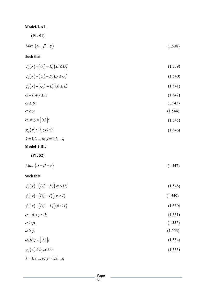
Page 61

Model-I-AL

(P1. 51)

Max

(1.538)

Such that

.T T Tk k k kf x U L U (1.539)

.I I Ik k k kf x U L U

(1.540)

.F F Fk k k kf x U L L

(1.541)

3;

(1.542)

;

(1.543)

;

(1.544)

, , 0,1 ;

(1.545)

; 0j jg x b x

(1.546)

1,2,.., ; 1,2,..,k p j q

Model-I-BL

(P1. 52)

Max

(1.547)

Such that


.I I Ik k k kf x U L L

(1.549)


(1.550)

3;

(1.551)

;

(1.552)

;

(1.553)

, , 0,1 ;

(1.554)

; 0j jg x b x

(1.555)

1,2,.., ; 1,2,..,k p j q

Page 62

And

Model-II-AL

(P1. 53)

Max

(1.556)

Subject to


.I I Ik k k kf x U L U

(1.558)


(1.559)

3;

(1.560)

;

(1.561)

;

(1.562)

, , 0,1 ;

(1.563)

; 0j jg x b x

(1.564)

1,2,.., ; 1,2,..,k p j q

Model-II-B

(P1. 54)

Max

(1.565)

Subject to


.I I Ik k k kf x U L L

(1.567)


(1.568)

3;

(1.569)

;

(1.570)

;

(1.571)

, , 0,1 ;

(1.572)

; 0j jg x b x

(1.573)

Page 63

1,2,.., ; 1,2,..,k p j q

1.31 Illustrated Numerical Example (P1. 55)

1 21 1 2 1 2,Min f x x x x

(1.574)

2 32 1 2 1 2, 2Min f x x x x (1.575)

Such that

1 2 1x x (1.576)

1 2, 0x x (1.577)

Solution : Here 1 6.75,TL 1 6.94TU 2 57.87,TL 2 60.78TU

Comparison of optimal solution by IFO and NSO Technique

Optimization Technique

Optimal Decision Variables

* *1 2,x x

Optimal Objective Functions

* *1 2,f f

Sum of Optimal Objective Values

Intuitionistic Fuzzy Optimization(IFO)

0.3659009 0.6356811

6.797078 58.79110

65.588178

Proposed Neutrosophic Optimization (NSO)

1 1, 0.019

2 2, 0.291 Model-I-AL

0.3704475 0.6315016

6.76957.87

64.63

Model-II-AL 0.3659010 0.634099

6.79758.59

65.38

Model-I-BL 0.3659016 0.6340984

6.79758.59

65.38

Model-II-BL 0.3659016 0.6340984

6.79758.59

65.38

Table 1.7 shows that neutrosophic optimization technique gives better result than Intuitionistic Fuzzy Nonlinear Programming Technique.

Page 64

The function of a riser is to supply additional molten metal to a casting to ensure a shrinkage porosity free casting.Shrinkage porosity occurs because of the increase in density from the liquid to solid state of metals.To be effective a riser must be solidify after casting and contain sufficient metal to feed the casting. Casting solidification time is predicted from Chvorinov‟s rule. Chvorinov‟s rule provides guidance on why risers are typically cylindrical.The longest solidification time for a given volume is the one where the shape of the part has the minimum surface area. From a practical standpoint cylinder has least surface area for its volume and easiest to make. Since the riser should solidify a cylinder side riser which consists of a cylinder of height H and diameter D. The theoretical basis for riser design is Chvorinov‟s rule which is

2/t k V SA where t solidification time (minutes/seconds), K solidification

constant for moulding material(minutes/in2 or seconds/cm2), V riser volume (in3 or cm3), SA cooling surface area of the riser.

The objective is to design the smallest riser such that R Ct t .where Rt solidification time of the riser, Ct solidification time of the casting,

2 2/ /R R R C C CK V SA K V SA (1.578)

The riser and casting are assumed to be moulded in the same material so that RK and CK are

equal .So / /R R C CV SA V SA . (1.579)

The casting has a specified volume and surface area, so

/C CV SA Y constant, (1.580)

which is called the casting modulus.

/ ,C CV SA Y (1.581)

2 / 4,R R RV D H (1.582)

22 / 4R R R RSA D H D (1.583)

Therefore

2 2/ 4 2 / 4 / 4 2R R R R R R R RD D H D D H H D Y (1.584)

We take 96CV cubic inch.

2 2.8 2.6 6.8 152CSA square inch. (1.585)

Then, 1 149 24 119 19R RD H (1.586)

Therefore Multi-objective cylindrical riser design problem can be stated as

1.32 Application of Neutrosophic Optimization in Riser Design Problem

Page 65

2, / 4R R R R RMinimize V D H D H

(1.587)

, / 4 2R R R R R R RMinimize t D H D H H D

(1.588)

Subject to 1 149 24 119 19R RD H

(1.589)

, 0R RD H

(1.383)

Here pay-off matrix is

42.75642 0.63157912.510209 0.6315786

R R

R

R

V TDH

Table 1.7 Values of Optimal Decision Variables and Objective Functions by Neutrosophic Optimization Technique

Optimal Decision variables

Optimal Objective Functions

Aspiration levels of Truth, Falsity and Indeterminacy Membership Functions

* 3.152158RD * 3.152158RH

* * *, 24.60870R R RV D H

* * *, 0.6315787R R Rt D H

* 0.1428574 * 0.1428574 * 0.00001

1.33 Neutrosophic Optimization(NSO) Technique to Solve

Minimization Type Multi-Objective Non-linear Programming

Problem(MONLP) A nonlinear multi-objective optimization problem is of the form

(P1. 56)

1 2, ,..., pMinimize f x f x f x (1.590)

1,2,...,j jg x b j q

(1.591)

Now the decision set nD , a conjunction of Neutrosophic objectives and constraints is defined

1 1

, ,n n n

p qn n n

k j D D Dk j

D G C x T x I x F x

(1.592)

Here

Page 66

1 2 3

1 2 3

, , ,...., ;min

, , ,....,

n n n np

n

n n n nq

G G G G

DC C C C

T x T x T x T xT x for all x X

T x T x T x T x

(1.593)

1 2 3

1 2 3

, , ,....., ;min

, , ,.....,

n n n np

n

n n n nq

G G G G

DC C C C

I x I x I x I xI x for all x X

I x I x I x I x

(1.594)

1 2 3

1 2 3

, , ,...., ;min

, , ,.....,

n n n np

n

n n n nq

G G G G

DC C C C

F x F x F x F xF x for all x X

F x F x F x F x

(1.595)

Where , ,n n nD D DT x I x F x are truth-membership function, indeterminacy membership

function, falsity membership function of neutrosophic decision set respectively .Now using

the definition of Smarandache‟s intersection of neutrosophic sets and criteria of decision

making (P1.56) is transformed to the non-linear programming problem as

Model-I-AN,BN

(P1. 57)

Max (1.596)

Max (1.597)

Min (1.598)

such that

;n

kGT x

(1.599)

;njC

T x

(1.600)

;nkG

I x

(1.601)

;njC

I x

(1.602)

;nkG

F x

(1.603)

;njC

F x

(1.604)

3; (1.605)

; ; (1.606)

, , 0,1

(1.607)

Here Model-I-AN and Model-I-BN stands for the algorithm with decreasing indeterminacy

nonlinear membership function and increasing indeterminacy nonlinear membership function

respectively.

Page 67

But as the decision makers needs to minimize indeterminacy membership function in real

world problem the above problem can be formulated as

Model-II-AN,BN

(P1. 58)

Max (1.608)

Min (1.609)

Min (1.610)

such that

;n

kGT x

(1.611)

;njC

T x

(1.612)

;nkG

I x

(1.613)

;njC

I x

(1.614)

;nkG

F x

(1.615)

;njC

F x

(1.616)

3; (1.617)

; ; (1.618)

, , 0,1

Here Model-II-AN and Model-II-BN stand for same as Model-I

Now this NLP problem (P1.57) and (P1.58) can be easily solved by an appropriate

mathematical programming to give solution of MONLP problem (P1.56) by NSO approach.


Step-1: Solve the MONLP problem (P1.56) as a single objective non-linear problem p times

for each problem by taking one of the objectives at a time and ignoring the others. These

solution are known as ideal solutions. Let kx be the respective optimal solution for the thk

different objective and evaluate each objective values for all these thk optimal solution.

Step-2: From the result of step-1, determine the corresponding values for every objective for

each derived solution; pay-off matrix can be formulated as follows

Page 68

* 1 1 11 2

2 * 2 21 2

*1 2

........

........

....... ........ ........ .......

.......

p

p

p p pp

f x f x f x

f x f x f x

f x f x f x

Step-3: For each objective kf x find lower bound TkL and the upper bound T

kU

*maxT rk kU f x (1.619)

*min 1,2,...,T rk kL f x where r k

(1.620)

For truth membership of objectives.

Step-4:We represent upper and lower bounds for indeterminacy and falsity membership of

objectives as follows :

1,2,......for k p Model-I,II-AL,AN

F Tk kU U (1.621)

;F T T Tk k k kL L t U L (1.622)

I Tk kL L (1.623)

I T T Tk k k kU L s U L (1.624)

Here ,t s are predetermined real numbers in 0,1 and for Model-I,II-BL,BN

F T Ik k kU U U

;F T T Tk k k kL L t U L

I T T Tk k k kL L s U L


Step-5: Define nonlinear truth membership, indeterminacy membership and falsity

membership functions as follows

1,2,.......,for k p

Page 69

1

1 exp

0

k

k

k k k

k k

k

Tk f x

Tkf x T T

k kf x f x f xT Tf x f x

Tf x

if f x L


U L

if f x U

(1.625)

For Model-I,II-AN

1

exp

0

k

k k k

k k

k

Ik f x

Ikf x I I

k kf x f x f xI If x f x

Ik f x

if f x L


U L

if f x U

(1.626)

For Model-I,II-BN

1

exp

0

k

k k k

k k

k

Ik f x

Ik f x I I


Ik f x

if f x U


U L

if f x L

(1.627)

0

1 1 tanh2 2 2

1

Ff x

F Ff x f x F F

f x f x f x f x

Ff x

if f x L


if f x U

(1.628)

Step-6:Now neutrosophic optimization method for MONLP problem gives a equivalent

nonlinear programming problem as:

Model-I-AN,BN

(P1. 59)

Maximize (1.629)

such that

;k kT f x

(1.630)

;k kI f x

(1.631)

;k kF f x

(1.632)

Page 70

3; (1.633)

; (1.634)

; (1.635)

, , 0,1 ;

(1.636)

j jg x b (1.637)

0,x

(1.638)

1,2,..., ;k p 1,2,...,j q (1.639)

Model-II-AN,BN

(P1. 60)

Maximize (1.640)

such that

;k kT f x

(1.641)

;k kI f x

(1.642)

;k kF f x

(1.643)

3; (1.644)

; (1.645)

; (1.646)

, , 0,1 ;

(1.647)

j jg x b (1.648)

0,x

(1.649)

1,2,..., ;k p 1,2,...,j q

Where Model-I,II-AN and Model-I,II-BN stands for the optimization algorithm with

decreasing indeterminacy nonlinear membership function and increasing indeterminacy

nonlinear membership function respectively.

which is reduced to equivalent nonlinear programming problem as

Model-I-AN

(P1. 61)

Maximize (1.650)

such that

Page 71

;4

T Tk k T

k k

U Lf x U

(1.651)

;2

k

k

T Tk k f

kf

U Lf x

(1.652)

; 1,2,....,k k

Tk f k ff x L for k p

(1.653)

1tanh 2 1 ,where

(1.654)

log 1

(1.655)

log (1.656)

4, (1.657)

6kf F F

k kU L

(1.658)

3; (1.659)

; (1.660)

; (1.661)

, , 0,1 ;

(1.662)

;j jg x b

(1.663)

0,x (1.664)

and

Model-I-BN

(P1. 62)

Maximize (1.665)

such that

;4

T Tk k T

k k

U Lf x U

(1.666)

;2

k

k

T Tk k f

kf

U Lf x

(1.667)

; 1,2,....,k k

T T Tk k k f k ff x U L L for k p

(1.668)

Page 72

1tanh 2 1 ,where

(1.669)

log 1

(1.670)

log (1.671)

4, (1.672)

6kf F F

k kU L

(1.673)

3; (1.674)

; (1.675)

; (1.676)

, , 0,1 ;

(1.677)

;j jg x b

(1.678)

0,x

This crisp nonlinear programming problem can be solved by appropriate mathematical

algorithm. Again according to decision makers choice the above problem also can be

formulated as

Model-II-AN

(P1. 63)

Maximize (1.679)

such that

;4

T Tk k T

k k

U Lf x U

(1.680)

;2

k

k

T Tk k f

kf

U Lf x

(1.681)

; 1,2,....,k k

Tk f k ff x L for k p

(1.682)

1tanh 2 1 ,where

(1.683)

log 1

(1.684)

log (1.685)

4, (1.686)

Page 73

6kf F F

k kU L

(1.687)

3; (1.688)

; (1.689)

; (1.690)

, , 0,1 ;

(1.691)

;j jg x b

(1.692)

0,x (1.693)

And

Model-II-B

(P1. 64)

Maximize (1.694)

such that

;4

T Tk k T

k k

U Lf x U

(1.695)

;2

k

k

T Tk k f

kf

U Lf x

(1.696)

; 1,2,....,k k

T T Tk k k f k ff x U L L for k p

(1.697)

1tanh 2 1 ,where

(1.698)

log 1

(1.699)

log (1.700)

4, (1.701)

6kf F F

k kU L

(1.702)

3; (1.703)

; (1.704)

; (1.705)

, , 0,1 ;

(1.706)

Page 74

;j jg x b

(1.707)

0,x

All the above crisp problems can be solved by appropriate optimization solver(LINGO).

1.34 Neutrosophic Goal Programming(NGP) Goal programming can be written as

(P1. 65)

Find

1 2, ,..., Tnx x x x

(1.708)

to achieve:

i iz t 1,2,...,i k (1.709)

subject to x X where it are scalars and represent the target achievement levels of the

objective functions that the decision maker wishes to attain provided, X is feasible set of

constraints.

The nonlinear goal programming problem can be written as

(P1. 66)

Find 1 2, ,..., Tnx x x x

(1.710)

so as to

iMinimize z with target value it ,acceptance tolerance ia ,indeterminacy tolerance id

rejection tolerance ic

(1.711)

x X (1.712)

j jg x b , 1,2,.....,j m (1.713)

0,ix 1,2,.....,i n (1.714)

with truth-membership, indeterminacy-membership and falsity-membership functions

1

1

0

i i

i i ii i i i i i

i

i i i

if z t

t a zT z if t z t aa

if z t a

(1.715)

Page 75

1

0

0

i i

i ii i i i

ii i

i i ii i i i i

i i

i i i

if z t

z t if t z t ad

I zt a z if t d z t a

a dif z t a

(1.716)

1

0

1

i i

i ii i i i i i

i

i i i

if z t

z tF z if t z t cc

if z t c

(1.717)

To maximize the degree of acceptance and indeterminacy and to minimize the degree of

rejection of objectives and constraints of nonlinear goal programming (NGP), let us consider

the following formulation,

(P1. 67)

, 1,2,....,iz iMaximize T z i k (1.718)

, 1,2,....,iz iMaximize I z i k

(1.719)

, 1,2,....,iz iMinimize F z i k

(1.720)

subject to

0 3, 1,2,....,i i iz i z i z iT z I z F z i k (1.721)

0, 0, 0 1,2,...,i i iz i z i z iT z I z F z i k

(1.722)

, 1,2,....,i iz i z iT z I z i k

(1.723)

, 1,2,...,i iz i z iT z F z i k

(1.724)

j jg x b , 1,2,...,j m

(1.725)

0,ix 1,2,...,i n (1.726)

where iz iT z ,

iz iI z and iz iF z are truth membership function indeterminacy

membership function ,falsity membership function of neutrosophic decision set respectively.

Now the NGP in model (P1.67) can be represented by crisp programming model using truth

membership, indeterminacy membership, and falsity membership functions as

(P1. 68)

Page 76

, ,Maximize Maximize Minimize (1.727)

, 1,2,...,iz iT z i k

(1.728)

, 1,2,...,iz iI z i k

(1.729)

, 1,2,...,iz iF z i k

(1.730)

, 1,2,.....,i iz t i k

(1.731)

0 3; (1.732) , 0, 1; (1.733)

, 1,2,.....,j jg x b j m

(1.734)

0, 1,2,....,ix i n

(1.735)

1.35 Theorem on Generalized Goal Programming For a generalized neutrosophic goal programming problem (P1.65)

The sum of truth, indeterminacy and falsity membership function will lie between 0 and

1 2 3w w w

Proof:

Let the truth ,indeterminacy and falsity membership functions be defined as

membership functions

1

1

1

0

i i

w i i ii i i i i i

i

i i i

w if z t

t a zT z w if t z t aa

if z t a

(1.736)

2

2

2

0

0

i i

i ii i i i

iwi i

i i ii i i i i

i i

i i i

if z t

z tw if t z t ad

I zt a zw if t d z t a

a dif z t a

(1.737)

33

3

0 i i

w i ii i i i i i

i

i i i

if z t

z tF z w if t z t cc

w if z t c

(1.738)

Page 77

Fig.-1.2 Truth Membership, Indeterminacy Membership and Falsity Membership

Function of iz

From Fig. -1.2 and definition of generalized single valued neutrosophic set it is clear that

10iz iT z w , 20

iz iI z w and 10iz iF z w

(1.739)

When i iz t

1iz iT z w and 0iz iI z and 0

iz iF z

(1.740)

Therefore 1 1 2 3i i iz i z i z iT z I z F z w w w w

(1.741)

and 1 0w implies that 0i i iz i z i z iT z I z F z

(1.742)

when ,i i i iz t t a from Fig.-1.2 we see that iz iT z and

iz iF z intersects each other and

the point whose coordinate is ,i i i it d d c .

where 1

1 2i

i i

wd w wa c

(1.743)

Now in the interval ,i i i iz t t d we see that

2 2 1 2 3i i i

i iz i z i z i

i

z tT z I z F z w w w w wd

(1.744)

Again in the interval ,i i i i iz t d t a

(1.745)

we see that 2 2 1 2 3i i i

i i iz i z i z i

i i

t a zT z I z F z w w w w wa d

. (1.746)

Also for i i i it z t a

(1.747)

when i iz t , 2 0i i iz i z i z iT z I z F z w

(1.748)

and 1 0i i iz i z i z iT z I z F z w

(1.749)

Page 78

and when i i iz t a , 1 1 1 2i i i

iz i z i z i

i

aT z I z F z w w w wc

(as 1i

i

ac ).

In the interval ( , ]i i i i iz t a t c

(1.750)

when i i iz t a , 2 2 0i i i

iz i z i z i

i

aT z I z F z w wc

(as 1i

i

ac ) (1.751)

and when i i iz t c , 1 1 2 3i i iz i z i z iT z I z F z w w w w

(1.752)

for i i iz t c , 3 1 2 3i i iz i z i z iT z I z F z w w w w (1.753)

and as 2 0w , 0i i iz i z i z iT z I z F z

(1.754)

Therefore combining all the cases we get

1 2 30

i i iz i z i z iT z I z F z w w w

(1.755)

Hence the proof.

1.36 Generalized Neutrosophic Goal Programming(GNGP) The Generalized Neutrosophic Goal Programming(GNGP) can be formulated as

(P1. 69)

, 1,2,....,iz iMaximize T z i k (1.756)

, 1,2,....,iz iMaximize I z i k

(1.757)

, 1,2,....,iz iMinimize F z i k

(1.758)

subject to

1 2 30 , 1,2,....,i i iz i z i z iT z I z F z w w w i k (1.759)

0, 0, 0 1,2,...,i i iz i z i z iT z I z F z i k

(1.760)

, 1,2,....,i iz i z iT z I z i k

(1.761)

, 1,2,...,i iz i z iT z F z i k

(1.762)

1 2 30 3w w w

(1.763)

1 2 3, , 0,1w w w

(1.764)

j jg x b , 1,2,...,j m

(1.765)

0,ix 1,2,...,i n (1.766)

Equivalently

Page 79


, 1,2,...,iz iT z i k

(1.768)

, 1,2,...,iz iI z i k

(1.769)

, 1,2,...,iz iF z i k

(1.770)

, 1,2,.....,i iz t i k

(1.771)

1 2 30 ;w w w

(1.772)

1 2 30, , 0, , 0, ;w w w

(1.773)

1 2 30,1 , 0,1 , 0,1 ;w w w

(1.774)

1 2 30 3;w w w

(1.775)

, 1,2,...,j jg x b j m

(1.776)

0, 1,2,...,jx j n

(1.777)

Equivalently

(P1. 70)


1

1 , 1,2,...,i i iz t a i kw

(1.779)

2

, 1,2,...,ii i

dz t i kw

(1.780)

2

, 1,2,...,i i i i iz t a a d i kw

(1.781)

3

, 1,2,...,ii i

cz t i kw

(1.782)

, 1,2,.....,i iz t i k

(1.783)

1 2 30 ;w w w

(1.784)

1 2 30, , 0, , 0, ;w w w

(1.485)

1 2 30,1 , 0,1 , 0,1 ;w w w

(1.786)

1 2 30 3;w w w

(1.787)

With the help of generalized truth, indeterminacy, falsity membership function the GNGP

based on arithmetic aggregation operator can be formulated as

Page 80

(P1. 71)

1 13

Minimize

(1.788)

subjected to same constraints as (P1.70)

With the help of generalized truth, indeterminacy, falsity membership function ,the GNGP

based on geometric aggregation operator can be formulated as

(P1. 72)

3 1 1Minimize (1.789)

subjected to same constraints as (P1.70).

Now this non-linear programming problem (P1.70 or P1.71 or P1.72) can be easily solved by

an appropriate mathematical programming to give solution of multi-objective non-linear

programming problem (P1.65) by GNGP approach.

1.37 Application of Neutrosophic Goal Programming to Bank Three

Investment Problem

Every investor must trade of return versus risk in deciding how to allocate his or her available funds. The opportunities that promise the greatest profits are almost the ones that present the most serious risks.Commercial banks must be especially careful in balancing return and risk because legal and ethical obligations demand that they avoid profit. This dilemma leads naturally the multi-objective optimization of investment that includes both profit and risk criteria.Our investment example [44] adopts this multi-objective approach to a fictitious Bank Three. Bank Three has a modest $20 million capital, with$150 million in demand deposits and$80 in times deposits(savings accounts and certificates of deposit).Table 1.8 display the categories among which the bank must divide its capital and deposited funds. Rates of return are also provided for each category together with other information related to risk.

Table 1.8 Bank Three Investment Opportunities

Investment Category, j

Return Rate(%) Liquid Part(%) Required Capital Asset(%)

Risk

Cash 0.0 100.0 0.0 No Short Term 4.0 99.5 0.5 No Government:1 to 5 years

4.5 96.0 4.0 No

Government:5 to 10 years

5.5 90.0 5.0 No

Government:over 10 years

7.0 85.0 7.5 No

Installment Loans

10.5 0.0 10.0 Yes

Page 81

Mortgage Loans 8.5 0.0 10.0 Yes Commercial Loans

9.2 0.0 10.0 Yes

The first goal of any private business is to maximize profit. Using rates of return from table 1,this produces objective functions

2 3 4 5 6 7 80.04 0.045 0.055 0.070 0.105 0.085 0.092Maximize I I I I I I I (Profit)

It is less clear how to quantify investment risk. We employ two common ratio measures. One is the capital –adequacy ratio, expressed as the ratio of required capital for bank solvency to actual capital. A low value indicates minimum risk. The “required capital” rates of table 1 approximate U.S. government formulas used to compute this ratio, and bank Three‟s present capital is$20 million. Thus we will express a second objective

2 3 4 5 6 7 81 0.005 0.040 0.050 0.075 0.100 0.100 0.10020

Minimize I I I I I I I

(1.559)

Another measure of risk focuses on illiquid risk assets. A low risk asset/capital ratio indicates a financially secure institution. For our example, this third measure of success is expressed as

6 7 8120

Minimize I I I

(1.790)

To complete a bank Three‟s investment plans, we must describe the relevant constraints

6.Investments must sum to the available capital and deposited funds.

7.Cash reserves must be at least 14% of demand deposits plus 4% of times deposits.

8.The portion of investments considered should be liquid at least 47% of demand deposits plus 36% of times deposits.

9.At least 30% of funds should be invested in commercial loans, to maintain the bank‟s community status.

Combining the 3 objective functions above with these 5 constraints completes a multi-objective linear programming model of Bank Three‟s Investment Problem.

(P1. 83)

1 2 8 2 3 4 5 6 7 8, ,..., 0.04 0.045 0.055 0.070 0.105 0.085 0.092Max PF I I I I I I I I I I

(Profit)(1.791)

1 2 8 2 3 4 5 6 7 81, ,..., 0.005 0.040 0.050 0.075 0.100 0.100 0.10020

Max CA I I I I I I I I I I

(Capital-Adequacy)(1.792)

Page 82

6 7 8 6 7 81, ,20

Max RA I I I I I I (Risk-Asset)(1.793)

Such that

1 2 8 1 2 3 4 5 6 7 81, ,..., 20150 8020

IA I I I I I I I I I I I (Invest All) (1.794)

1 1 0.14 150 0.04 80CR I I (Cash Reserve) (1.795)

1 2 5 1 2 3 4 5, ,..., 1.00 0.995 0.960 0.900 0.850 0.47 150 0.36 80L I I I I I I I I

(Liquidity) (1.796)

0.05 20 150 80j jCD I for all 1,2,..,8j (Diversification) (1.797)

8 0.30 20 150 80C I (Commercial) (1.798)

1 2 8, ,..., 0I I I

(1.799)

1.38 Numerical Example

Let us consider the input values of membership functions as follows'

1 1 1 1 112, 6.67, 3, 13, 5.67c a t c p '2 2 2 2 20.58, 0.22, 0.20, 0.60, 0.20c a t c p

'3 3 3 3 35, 1.5, 1.0, 5.5, 1.0c a t c p

The optimal Bank Three‟s Investment Problem can be tabulated as

Table 1.9 Goal Programming Solution of Bank Three Problem Weights Optimal Primal Variables Optima Objectives

1 0.8w 2 0.1w

3 0.1w 1 24.2,x 2 12.5,x

3 12.5,x 4 12.5,x

5 46.37,x 6 53.43,x

7 12.5,x 8 24.2x

1 18.67363,f

2 0.942915,f 3 7.096f

1 0.05w 2 0.9w

3 0.05w 1 100,x 2 12.5,x

3 12.5,x 4 12.5,x

5 12.5,x 6 12.5,x

7 12.5,x 8 75x

1 11.9,f 2 0.60625,f

3 5.00f

1 0.1w 2 0.1w

3 0.8w 1 24.2,x 2 88.30,x

3 12.5,x 4 12.5,x

5 12.5,x 6 12.5,x

7 12.5,x 8 75x

1 14.932,f 2 0.6252,f

3 5.00f

1 1/ 3w 2 1/ 3w 1 24.2,x 2 88.30,x 1 14.932,f 2 0.6252,f

Page 83

3 1/ 3w 3 12.5,x 4 12.5,x

5 12.5,x 6 12.5,x

7 12.5,x 1 75x

3 5.00f

Table 1.10 Lexicographic Goal Programming Solution of Bank Three Problem

Optimal Primal Variables Optima Objectives 1 24.2,x 2 22.51454,x

3 12.5,x 4 12.5,x

5 34.64474,x

6 56.14072,x 7 12.5,x

8 24.2x

1 18.43299,f

2 0.9100,f

3 7.182036f

1.39 Neutrosophic Non-linear Programming (NNLP) Optimization

to solve Parameterized Multi-objective Non-linear Programming

Problem (PMONLP)

A Multi-Objective Neutrosophic Non-Linear Programming(MONNLP) Problem with imprecise co-

efficient can be formulated as

(P1. 84)

0

0

0 0 01 1

kk tj

T nan n

k k t k t jt j

Minimize f x c x

for 0 1,2,....,k p (1.800)

Such that 1 1

iitj

T nan n n

i it it j i it j

f x c x b

for 1,2,....,i m (1.801)

0jx 1,2,...,j n (1.802)

Here 0

,k t ,it i are the signum functions used to indicate sign of term in the equation. 0

0,k tc

0itc .0

,k tja itja are real numbers for all 0, , , .i t k j

Here

0 0 0 0 0 0 0 0 0 0 0 0 0

1 2 3 1 2 3 1 2 3, , ; , , ; , , ; ;n T T I I F Fk t k t k t k t k t k t k t k t k t k t k t k t k tc c c c w c c c c c c

(1.803)

1 2 3 1 2 3 1 2 3, , ; , , ; , , ; ;n T T I I F Fit it it it it it it it it it it it itc c c c w c c c c c c (1.804)

1 2 3 1 2 3 1 2 3, , ; , , ; , , ;n T T I I F Fi i i i i i i i i i i i ib b b b w b b b b b b (1.805)

Using total integral value of truth, indeterminacy and falsity membership functions we transform

above MONNLP with imprecise parameter as

(P1. 85)

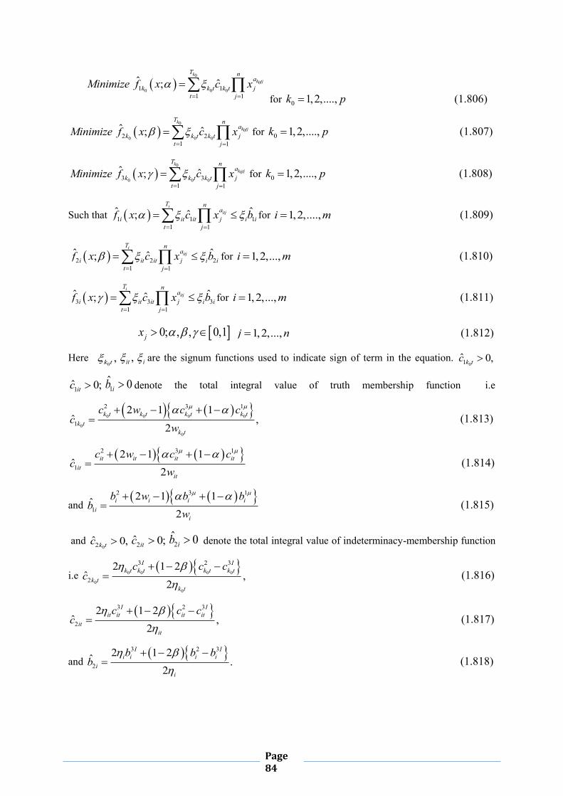
Page 84

0

0

0 0 01 11 1

ˆ ˆ;k

k tj

T na

k k t k t jt j

Minimize f x c x

for 0 1,2,....,k p (1.806)

0

0

0 0 02 21 1

ˆ ˆ;k

k tj

T na

k k t k t jt j

Minimize f x c x

for 0 1,2,....,k p

(1.807)

0

0

0 0 03 31 1

ˆ ˆ;k

k tj

T na

k k t k t jt j

Minimize f x c x

for 0 1,2,....,k p

(1.808)

Such that 1 1 11 1

ˆ ˆˆ;i

itj

T na

i it it j i it j

f x c x b

for 1,2,....,i m (1.809)

2 2 21 1

ˆ ˆˆ;i

itj

T na

i it it j i it j

f x c x b

for 1,2,...,i m (1.810)

3 3 31 1

ˆ ˆˆ;i

itj

T na

i it it j i it j

f x c x b

for 1,2,...,i m (1.811)

0; , , 0,1jx 1,2,...,j n (1.812)

Here 0

,k t ,it i are the signum functions used to indicate sign of term in the equation. 01̂ 0,k tc

1̂ 0;itc 1̂ 0ib denote the total integral value of truth membership function i.e

0 0 0 0

0

0

2 3 1

1

2 1 1ˆ ,

2k t k t k t k t

k tk t

c w c cc

w

(1.813)

2 3 1

1

2 1 1ˆ

2it it it it

itit

c w c cc

w

(1.814)

and 2 3 1

1

2 1 1ˆ2

i i i ii

i

b w b bb

w

(1.815)

and 02ˆ 0,k tc 2ˆ 0;itc 2̂ 0ib denote the total integral value of indeterminacy-membership function

i.e 0 0 0 0

0

0

3 2 3

2

2 1 2ˆ ,

2

I Ik t k t k t k t

k tk t

c c cc

(1.816)

3 2 3

2

2 1 2ˆ ,

2

I Iit it it it

itit

c c cc

(1.817)

and 3 2 3

2

2 1 2ˆ .2

I Ii i i i

ii

b b bb

(1.818)

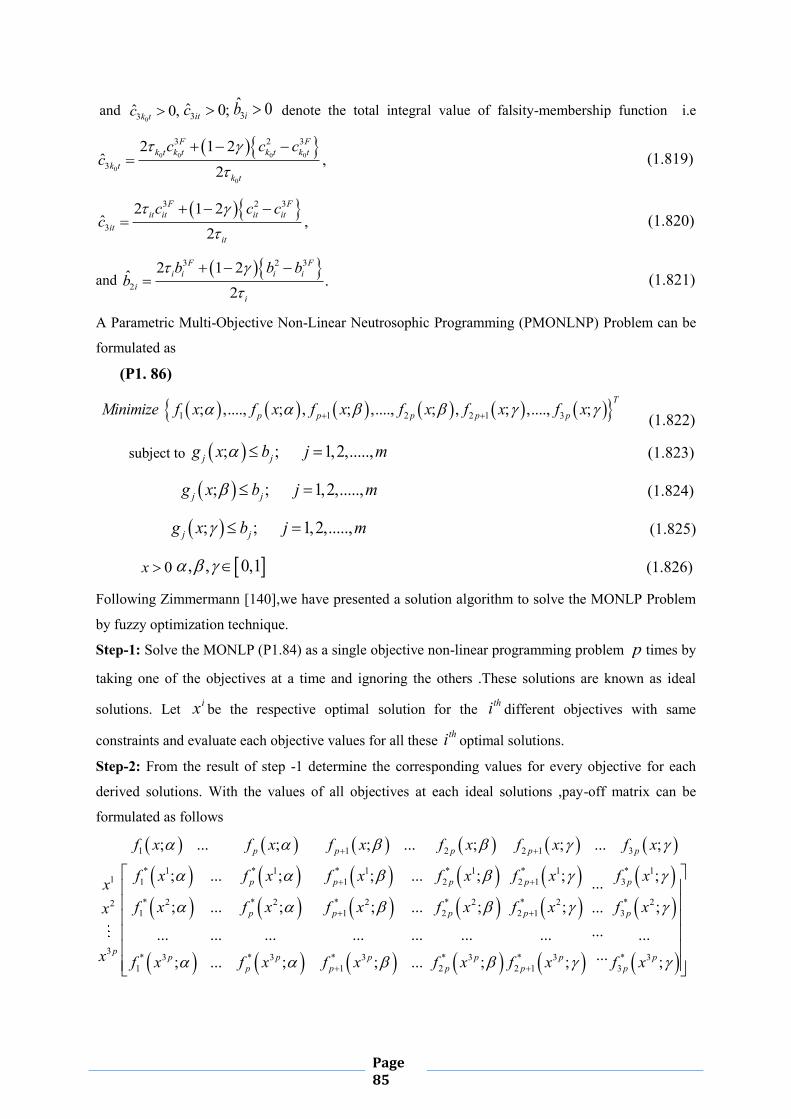
Page 85

and 03̂ 0,k tc 3̂ 0;itc 3̂ 0ib denote the total integral value of falsity-membership function i.e

0 0 0 0

0

0

3 2 3

3

2 1 2ˆ ,

2

F Fk t k t k t k t

k tk t

c c cc

(1.819)

3 2 3

3

2 1 2ˆ ,

2

F Fit it it it

itit

c c cc

(1.820)

and 3 2 3

2

2 1 2ˆ .2

F Fi i i i

ii

b b bb

(1.821)

A Parametric Multi-Objective Non-Linear Neutrosophic Programming (PMONLNP) Problem can be

formulated as

(P1. 86)

1 1 2 2 1 3; ,...., ; , ; ,...., ; , ; ,...., ;T

p p p p pMinimize f x f x f x f x f x f x

(1.822)

subject to ; ; 1,2,.....,j jg x b j m

(1.823)

; ; 1,2,.....,j jg x b j m

(1.824)

; ; 1,2,.....,j jg x b j m

(1.825)

0x , , 0,1

(1.826)

Following Zimmermann [140],we have presented a solution algorithm to solve the MONLP Problem

by fuzzy optimization technique.

Step-1: Solve the MONLP (P1.84) as a single objective non-linear programming problem p times by

taking one of the objectives at a time and ignoring the others .These solutions are known as ideal

solutions. Let ix be the respective optimal solution for the thi different objectives with same

constraints and evaluate each objective values for all these thi optimal solutions.

Step-2: From the result of step -1 determine the corresponding values for every objective for each

derived solutions. With the values of all objectives at each ideal solutions ,pay-off matrix can be

formulated as follows

1 1 2 2 1 3

* 1 * 1 * 1 * 1 * 11 1 1 2 2 1

* 2 * 2 * 2 * 221 1 2 2

3* 3 * 3 * 3 * 3

1 1 2

; ... ; ; ... ; ; ... ;

; ... ; ; ... ; ;

; ... ; ; ... ;

... ... ... ... ... ...

; ... ; ; ... ;

p p p p p

p p p p

p p p p

pp p p p

p p p

f x f x f x f x f x f x

f x f x f x f x f xxf x f x f x f x fx

x f x f x f x f x

* 13

* 2 * 21 3

* 3 * 32 1 3

;...; ;...

...... ......; ;

p

p

p pp p

f x

x f x

f x f x

Page 86

Here 1 2 3, ,......, px x x are the ideal solutions of the objectives

1 2 1 2 2 2 1 2 2 3; , ; ,...., ; , ; , ; ,...., ; , ; , ; ,...., ;p p p p p p pf x f x f x f x f x f x f x f x f x

respectively.

Step-3: For each objective ; , ; , ;k k kf x f x f x find lower bound TkL and the upper bound

TkU ,

* *max ;T rk kU f x p

(1.827)

and

* * *min ; , , ; 1,2,...,3T r

k kL f x p where p k p (1.828)

for truth membership of objectives.

Step-4:We represent upper and lower bounds for indeterminacy and falsity membership of objectives

as follows :

(1.829)

(1.830)

Here are predetermined real numbers in

Step-5: Define truth membership, indeterminacy membership and falsity membership functions as

follows

1

1 exp

0

k

k

k k k

k k

k

Tk f x

Tkf x T T

k kf x f x f xT Tf x f x

Tf x

if f x L


U L

if f x U

(1.831)

1

exp

0

k

k k k

k k

k

Ik f x

Ikf x I I


Ik f x

if f x L


U L

if f x U

(1.832)

1,2,....,3for k p

;F T F T T Tk k k k k kU U and L L t U L

I T I T T Tk k k k k kL L and U L s U L

,t s 0,1

1,2,..,3for k p

Page 87

0

1 1 tanh2 2 2

1

Ff x

F Ff x f x F F

f x f x f x f x

Ff x

if f x L


if f x U

(1.833)

Where (1.834)

, (1.835)

Step-6:Now NSO method for MONLP problem with probabilistic operator gives an equivalent

nonlinear programming problem as:

(P1. 87)

2 3

1 1 2 1

; ; ;p p p

i i i i i ii i p i p

Maximize T f x T f x T f x

(1.836)

2 3

1 1 2 1

1 ; 1 ; 1 ;p p p


Minimize I f x I f x I f x

(1.837)

2 3

1 1 2 1

1 ; 1 ; 1 ;p p p


Minimize F f x F f x F f x

(1.838)

0 ; ; ; 3i i i i i iT f x I f x F f x (1.839)



; ;j jg x b ; ;j jg x b ; ;j jg x b (1.842)

, , 0,1 (1.843)

1,2,.., ;i p 1,2,...,j m

This crisp nonlinear programming problem can be solved by appropriate mathematical algorithm.

1.40 Neutrosophic Optimization Technique(NSO) to solve

Parametric Single-Objective Non-linear Programming Problem

(PSONLP)

A single-objective neutrosophic NLP problem with imprecise co-efficient can be formulated

as

6k F F

k kU L

4

subject to

0x

Page 88

(P1. 88)

(1.844)

Such that for (1.845)

(1.846)

Here are the signum functions used to indicate sign of term in the equation.

. are real numbers for all

Here (1.847)

(1.848)

(1.849)

for neutrosophic number coefficient. Using nearest interval approximation method ,we

transform all the triangular neutrosophic number into interval number i.e

and

Now the Single-Objective Neutrosophic Programming(SONSP) with imprecise parameter is

of the following form

(P1. 89)

(1.850)


(1.852)

Here are the signum function used to indicate sign of term in the equation.

denote the interval component i.e and

and

are real numbers for all

Using parametric interval valued function the above problem transform into

(P1. 90)

(1.853)

1 1

tjnT

ant t j

t j

Minimize f x c x

1 1

iitj

T nan n

i it it j i it j

f x c x b

1,2,....,i m

0jx 1,2,....,j n

,t ,it i 0,tc

0itc ,tja itja , , .i t j

1 2 3 1 2 3 1 2 3, , ; , , , ; , , ;t t t

n T T T I I I F F Ft t t t c t t t c t t t cc c c c w c c c c c c

1 2 3 1 2 3 1 2 3, , ; , , , ; , , ;it it it

n T T T I I I F F Fit it it it c it it it c it it it cc c c c w c c c c c c

1 2 3 1 2 3 1 2 3, , ; , , , ; , , ;i i i

n T T T I I I F F Fi i i i b i i i b i i i bb b b b w b b b b b b

, ,L Ut tc c , ,L U

it itc c

,L Ui ib b

0

1 1

ˆ ˆ tjnT

ak t t j

t j

Minimize f x c x

1 1

ˆ ˆˆi

itj

T na

i it it j i it j

f x c x b

1,2,....,i m

0jx 1,2,....,j n

,t ,it i ˆ 0,tc

ˆ 0;itc ˆ 0ib ˆ , ,L Ut t tc c c ˆ , ,L U

it it itc c c ˆ ,L Ui i ib b b

,tja itja , , .i t j

1

1 1

; tjnT s s aL U

t t t jt j

Minimize f x s c c x

Page 89


(1.855)

Here are the signum functions used to indicate sign of term in the equation.

Let us consider a Single-Objective Nonlinear Optimization Problem(SONLOP) as

(P1. 91)

(1.856)

(1.857)

(1.858)

Usually constraint goals are considered as fixed quantity .But in real life problem ,the


type constraints at least and it may possible to extend to .This fact seems

to take the constraint goal as a NS and which will be more realistic descriptions than others.

Then the NLP becomes NSO problem with neutrosophic resources, which can be described

as follows

(P1. 92)

(1.859)

(1.860)

(1.861)

To solve the NSO (P1.92), following Werner‟s [118] and Angelov [3] we are presenting a

solution procedure for SONSO problem as follows

Step-1: Following Werner‟s approach solve the single objective non-linear programming

problem without tolerance in constraints (i.e ),with tolerance of acceptance in

constraints (i.e ) by appropriate non-linear programming technique

Here they are

(P1. 93)

Sub-problem-1

(1.862)

1 1

1 1

;i

itj

T ns s s saL U L Ui it it it j i i i

t j

f x s c c x b b

1,2,....,i m

0jx 1,2,....,j n 0,1s

,t ,it i

;Minimize f x s

; 1,2,......,j jg x s b s j m

0x 0,1s

jb s 0j jb s b s

;Minimize f x s

; 1,2,....,nj jg x s b s j m

0x 0,1s

;j jg x s b s

0;j j jg x s b s b s

;Minimize f x s

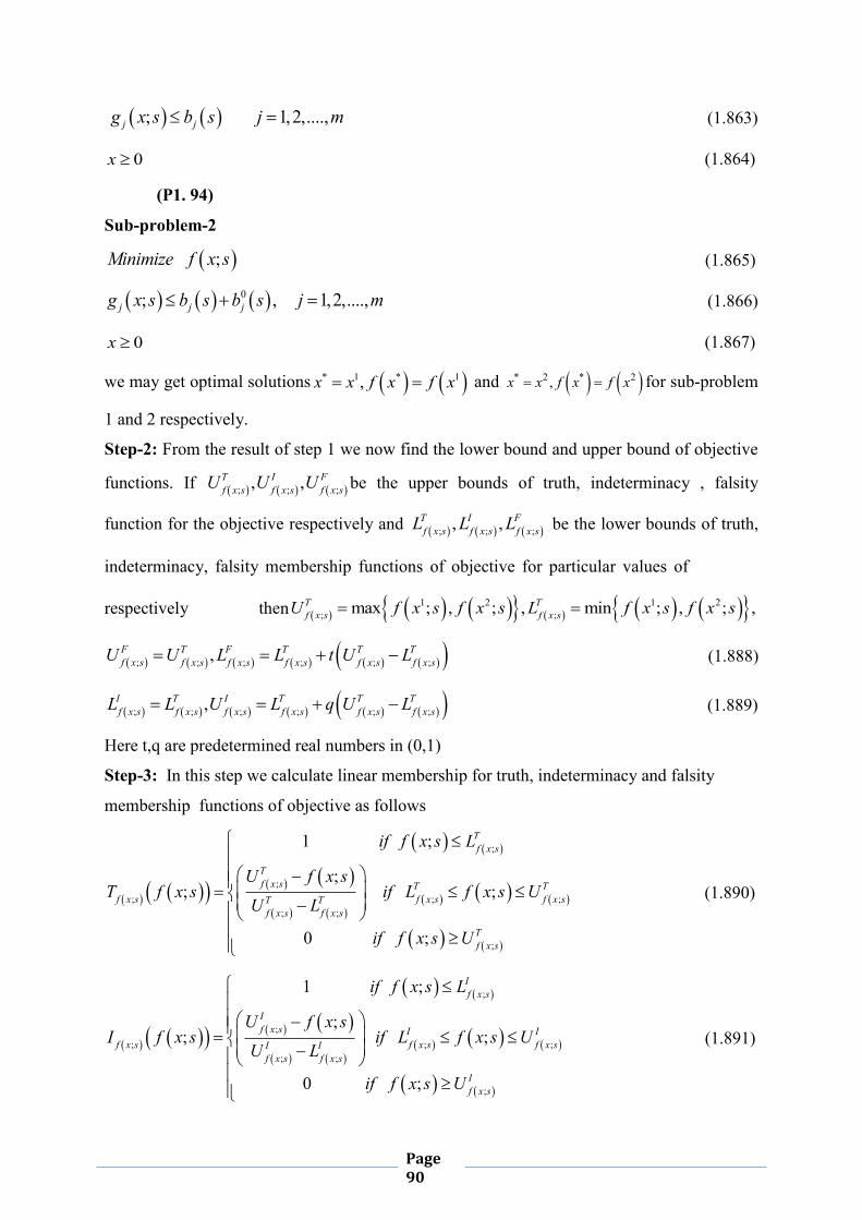
Page 90

(1.863)

(1.864)

(P1. 94) Sub-problem-2

(1.865)

(1.866)

(1.867)

we may get optimal solutions and for sub-problem

1 and 2 respectively.


functions. If be the upper bounds of truth, indeterminacy , falsity

function for the objective respectively and be the lower bounds of truth,

indeterminacy, falsity membership functions of objective for particular values of

respectively then

(1.888)

(1.889)

Here t,q are predetermined real numbers in (0,1)

Step-3: In this step we calculate linear membership for truth, indeterminacy and falsity

membership functions of objective as follows

(1.890)

(1.891)

; 1,2,....,j jg x s b s j m

0x

0,1s

;Minimize f x s

0; , 1,2,....,j j jg x s b s b s j m

0x

0,1s

* 1 * 1,x x f x f x * 2 * 2,x x f x f x

; ; ;, ,T I Ff x s f x s f x sU U U

; ; ;, ,T I Ff x s f x s f x sL L L

0,1s

1 2 1 2; ;max ; , ; , min ; , ; ,T T

f x s f x sU f x s f x s L f x s f x s

; ; ; ; ; ;,F T F T T Tf x s f x s f x s f x s f x s f x sU U L L t U L

; ; ; ; ; ;,I T I T T Tf x s f x s f x s f x s f x s f x sL L U L q U L

;

;; ; ;

; ;

;

1 ;

;; ;

0 ;

Tf x s

Tf x s T T

f x s f x s f x sT Tf x s f x s

Tf x s

if f x s L

U f x sT f x s if L f x s U

U L

if f x s U

;

;; ; ;

; ;

;

1 ;

;; ;

0 ;

If x s

If x s I I

f x s f x s f x sI If x s f x s

If x s

if f x s L

U f x sI f x s if L f x s U

U L

if f x s U

Page 91

(1.892)

Step-4: In this step using linear function for truth, indeterminacy and falsity membership

functions, we may calculate membership function for constraints as follows

(1.893)

(1.894)

(1.895)

where and for .

Step-5: Now using NSO for single objective optimization technique the optimization

problem (P1.92) can be formulated as

(P1. 95)

(1.896)

such that

(1.897)

(1.898)

(1.899)

(1.900)

;

;; ; ;

; ;

;

0 ;

;; ;

1 ;

Ff x s

Ff x s F F

f x s f x s f x sF Ff x s f x s

Ff x s

if f x s L

f x s LF f x s if L f x s U

U L

if f x s U

00

; 0

0

1 ;

;; ;

0 ;

j

j j

j j jj j j j jg x s

j

j j

if g x s b

b s b s g x sT g x s if b s g x s b s b s

b

if g x s b s

;

; ;;

;

1 ;

;; ;

0 ;

j

j j

j

j

j j

j jg x sj j j jg x s g x s

g x s

j j g x s

if g x s b s

b s g x sI g x s if b s g x s b s

if g x s b s

;

; 0; ;0

;

0

0 ;

;; ;

1 ,

j

j

j j

j

j j g x s

j j g x sj j j j jg x s g x s

j g x s

j j j

if g x s b s

g x s b sF g x s if b s g x s b s b s

b s

if g x s b s b s

1,2,....., , 0,1j m t q

Maximize

; ; ;f x sT x s

; ;jgT x s

,; ;

f x sI x s

; ;jgI x s

;; ;

f x sF x s

Page 92

(1.901)

(1.902)

(1.903)

, , 0,1 (1.904)

Now the above problem (P1.95) can be simplified to following crisp linear programming


(P1. 96)

(1.905)

(1.906)

(1.907)

(1.908)

(1.909)

(1.910)

(1.911)

(1.912)

(1.913)

(1.914)

; ;jgF x s

3;

; ;

0,1s

Maximize

; . ;T T Tsuch that f x s U L U

; ; ;; . ;I I If x s f x s f x sf x s U L U

; ; ;; .F F Ff x s f x s f x sf x s U L L

3;

; ;

; . ;T T Tjg x s U L U

; ; ;; . ;j j j

I I Ij g x s g x s g x sg x s U L U

; ; ;; .j j j

F F Fj g x s g x s g x sg x s U L L

, , 0,1 0,1s 1,2,....,j m

Page 93

Page 94

CHAPTER 2Structural Design Optimization

Optimization or in other word mathematical programming is the collection of mathematical

principles and methods that have been used for solving several problems in many disciplines,

including physics, biology, engineering, economics etc. Engineering is a branch of science

where engineers are engaged in formulating different designs with useful objectives. As for

examples civil engineers Designs Bridge, pavement and building, mechanical engineers

design welded beam design, an electrical engineer designs computer, a chemical engineers

design a chemical process. To deal with competitive market place an engineer might not only

be interested in design which works at some sort of nominal level but is the best design in

some way. The process of determining the best design is called optimization.

In mechanics a structure is defined by J.E.Gordon as “any assemblage of materials which is

intended to sustain loads”. The structural optimization is the subject of making an assemblage

of materials sustains loads in the best way. As for example, let us consider the situation where

load is to be transmitted from a region in space to a fixed support in best possible way .Then

first specification that comes to our mind to make the structure as light as possible, i.e to

minimize weight, secondly stiff as possible and another idea that could be to make it as

insensitive to buckling or instability as possible. In case of welded beam design the welding

is process of joining metallic parts with the application of heat or pressure or the both, with or

without added material. This efficient method for obtaining permanent joints in metallic parts

are generally used as a substitute for riveted joint or can be used as an alternative method for

casting and forging. Above all, the design of welded beam should be economical (i.e the

welding cost is to minimize) and durable one. Similarly Highway construction agencies

throughout the globe chasing accelerating demands on durable un dowelled jointed plain

concrete pavement (JPCP) due to scanty of rehabilitation of the same. Since decades,

different design methods had been developed by various organizations which suit their locale

and fix the depth criteria of the JPCP along with other parameters by satisfying the standard

code of practice but few of them tries to optimize the design thickness of the same. Moreover

few approaches designed such thickness of cited pavement by considering traffic overloading

condition, its fatigue life and the fluctuation of ambient temperature effect individually. So

Page 95

during service life of such pavement, the traffic loads and adverse environmental effect

would deteriorate its joints and ultimately its foundation. Therefore optimization of such rigid

pavement become essential considering multiple decision making criteria as stated above to

make it more durable.

Now such structural optimization and pavement design optimization i.e maximization or

minimization cannot be performed without any constraints. For example if there is no

limitation of the amount of the material that can be used, the structure can be made stiff

without limit and we have an optimization problem without a well-defined solution. So

constraints are necessary. Quantities that are usually constrained in structural optimization

problem and welded beam design problem are stresses, deflection, buckling load, and or the

geometry. The factors governing of JPCP constraints such as fatigue analysis, stresses and

deflections , axel loads, pavement thickness, modulus of elasticity of cement concrete,

subgrade modulus, Poisson‟s ratio, load contact area, annual rate of growth of commercial

traffic, number of axel per day, radius of relative stiffness , design period and so on.

Thus we can formulate a optimization problem by picking one of the measures on structural

performances as weight, stiffness, critical load, stress, displacement, deflection, geometry or

cost of welding or thickness of JPCP as an objective function that should be maximized or

minimized and some other measures as constraints. This type of optimization problem is

called single objective optimization problem. But there is some optimization problem where

multiple and conflicting objectives frequently exists .The accomplishment of this task is due

to the methodology known as multi-objective optimization.

But in the real world, uncertainty or vagueness is prevalent in Engineering Computations. In

the context of structural engineering and mechanical engineering design the uncertainty is

connected with lack of accurate data of design factors. In case of pavement design several

design methods e.g. American Association of State Highway and Transportation

Officials(AASHTO), Portland Cement Association (PCA) Method Crop of Engineers of the

US army iteration method etc. are available to determine the thickness of JPCP. However all

such methods follow numerous monographs, tables and charts to do the same and abiding by

certain loop of algorithm in the cited iteration process to find an effective thickness of such

pavement. But most of the time, designers stop the cited procedure even after two or three

trials which yield safe but unnecessarily less economical thick rigid pavement.

So lots of efforts had been made to get rid of from such problem. As for example finite

element method and genetic Algorithm type of crisp optimization method had been applied

on the cited subject, where the values of the input parameters were obtained from

Page 96

experimental data in laboratory scale. Sometimes the above cited standards have already

ranged the magnitude of those parameters in between maximum to the minimum value.

Therefore, designer get confused to select those input parameters from such ranges which

yield imprecise parameters with three key governing factors i.e. degree of acceptance,

rejection and hesitancy that attributes the necessity of Fuzzy Set (FS)theory, Intuitionistic

Fuzzy Set (IFS) theory and Neutrosophic Set (NS) theory For this purpose we will optimize

captioned optimum design in imprecise environment.

2.1 S.I Unit Prefixes

Prefix Symbol Multiplication Factor

Tera T 1210

Giga G 910

Mega M 610

Kilo K 310

Hector h 210

Deka da 110

Deci D 110

Centi c 210

Milli m 310

Micro 610

Nano n 910

Pico p 1210

2.2 Conversion of U.S Customary Units to S.I Units

Quantity Conversion of U.S

Customary Unit to S.I. Units

Conversion of S.I. Units to U.S Customary Units

Length 1 . 25.4 0.0254in mm m

1 . 304.8 0.3048ft mm m 1 0.039370mm in

1 39.370 3.281m in ft Area 2 21 . 645.16in mm 2 21 0.001550mm in

Page 97

2 21 . 0.09290304ft m 2 2 21 1550 10.764m in ft Volume 3 31 . 16387.064in mm

3 31 . 0.028317ft m

3 31 0.000061024mm in 3 31 35.315m ft

Force 1 4.45lb N 1 0.2248N lb Stress

21 6890 , 1 1 Npsi Pa Pam

1 0.000145Pa psi

Conversion of 525 10 N

mm to 21 1 NGPa Pa

m

59

522

5 10105 10 500

1000

GNN Gpa

mm m

(2.1)

Conversion of 27 Nmm

to Mpa

6

22 2

7107 7 7

1000

MNN MN Mpa

mm mm

(2.2)

A tensile bar stretches an amount . ,.

P LA E

where is the applied force, L is the length of

the bar , A is the cross sectional area, and E is the Young’s Modulus. The bar has a circular cross section. Given a load of 60 ,KN a length of 70 ,cm a diameter of , 5mm and a Young’s Modulus of 207 ,Gpa calculate the deflection in mm

3

2 22 92

2

4 60 10 70 10. . 4 4 60 70. 105 207 5 207.

2

N mmP L P L PL KN cmA E d E Nd mm Gpa mmE

m

3

92

2

4 60 10 70 1011.81

105 207

1000

N mmmm

Nmmmm

(2.3)

2.3 Design Studies In this book we have considered Two-bar truss design, three bar truss design, Jointed plain

concrete pavement design and Welded Beam design as structural optimization models. Their

formulation have been generated in the following way

Page 98

2.3.1 Two-Bar Truss(Model-I) A well-known two-bar [Fig.-2.1] planar truss structure is considered. The design objective is

to minimize weight of the structural 1 2, , BWT A A y of a statistically loaded two-bar planar

truss subjected to stress 1 2, ,i BA A y constraints on each of the truss members 1,2i .

Fig.-2.1 Two-Bar Planar Truss(Model-III)

Optimization model of two-bar truss shown in Fig.-1.1 is designed to support the loading

condition. The weight of the structure is

1 1 2 2 ,WT A L A L

(2.4)

where is the material density of the bar 1 2,A A are the cross sectional area and 1 2,L L are the

length of bar 1and bar 2 respectively. Length ,AC l Perpendicular distance from AC to

point load point B is ,Bx Nodal load P .Using simple Pythagorean‟s theorem we may find

the length of the each bars

22

1 ,B BL x l y (2.5)

2 22 B BL x y . (2.6)

Therefore weight of the structure is

22 2 2

1 2B B B BWT A x l y A x y

. (2.7)

Let 1P and 2P be the reaction forces along the bar 1and bar 2 respectively .Considering the

equilibrium condition at loading point, the following equations are obtained

1 1 2 2cos cos ,P P P (2.8)

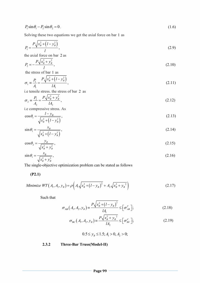
Page 99

1 1 2 2sin sin 0P P . (1.6)

Solving these two equations we get the axial force on bar 1 as

2 2

1 ,B BP x l y

Pl

(2.9)

the axial force on bar 2 as

2 2

2 ,B BP x yP

l

(2.10)

the stress of bar 1 as

2 2

11

1 1

,B BP x l yP

A lA

(2.11)

i.e tensile stress. the stress of bar 2 as

2 22

22 2

,B BP x yPA lA

(2.12)

i.e compressive stress. As

1 2 2

cos ,B

B B

l y

x l y

(2.13)

1 2 2

sin ,B

B B

x

x l y

(2.14)

2 2 2cos ,B

B B

yx y

(2.15)

1 2 2sin ,B

B B

xx y

(2.16)

The single-objective optimization problem can be stated as follows

(P2.1)

22 2 21 2 1 2, , B B B B BMinimize WT A A y A x l y A x y (2.17)

Such that

22

AB 1 21

, , ;B B TB AB

P x l yA A y

lA

(2.18)

2 2

BC 1 22

, , ;B B CB BC

P x yA A y

lA

(2.19)

1 20.5 1.5; 0, 0;By A A

2.3.2 Three-Bar Truss(Model-II)

Page 100

A well-known three bar planer truss is considered in Fig2.2 to minimize weight of the

structure 1 2,WT A A and minimize the deflection 1 2,A A at a loading point of a

statistically loaded three bar planer truss subject to stress constraints on each of the truss

members

Fig.-2.2 Three-Bar Planar Truss(Model-I)

Consider the three-bar truss shown in Fig-2.2. The bars have Young‟s modulus E and the

lengths are 1 2 3l l l L .The design variables are cross-sectional areas 1 2,A A and 3A .But we

assume that 1 3A A .Weight of the structure is

1 1 2 2 3 3 1 22 2WT l A l A l A L A A

(2.20)

where is the material density of each bar. The equilibrium equations in the direction x- and

y- directions become in matrix form

1

2

3

1 102 2

1 1 12 2

x

y

NP

NP

N

(2.21)

i.e TF B N .Where F represents the column matrix of external load, N represents the

column matrix of member‟s forces, TB and represents the diagonal matrix of member of

stiffness. We cannot obtain bar forces from equilibrium equations alone since the number of

bars exceeds the number of degree-of-freedom. In order to find the bar forces, or, rather, that

appear in the constraints, we need to make use of Hook‟s law and geometry conditions. The

extension of each bar corresponding to length and force are given in Table 2.1.

Table 2.1 Extension of Bars of Fig.-2.2

Bar Length Force Extension

Bar1 1 2l L 1N 1

11

2N LeA E

Page 101

Bar2 2l L 2N 2

22

N LeA E

Bar3 3 2l L 3N 3

31

2N LeA E

we have 1,2,3i ii

i

EAeN il

(2.22)

1 11 1

12 2

2 2 2

3 3 33 1

2 2,

22

e A E e ALN

e A E EN e AL L

N e Ae A EL

(2.23)

1

1 1

2 2 2

3 1 3

0 02

0 0

0 02

AN e

EN A eL

N A e

(2.24)

We write these equations for all three bars in matrix form as N De , where 1

2

1

0 02

0 0 ,

0 02

A

ED AL

A

(2.25)

1

2

3

,N

N NN

(2.26)

1

2

3

ee e

e

(2.27)

The compatibility equations relate the member displacement e to the nodal displacement r by

,e Br the bar forces are obtained as ,N DBr s, .The equilibrium equation

1,2,3i ii

i

EAeN il

(2.28)

becomes T TF B N B DBr Kr (2.29)

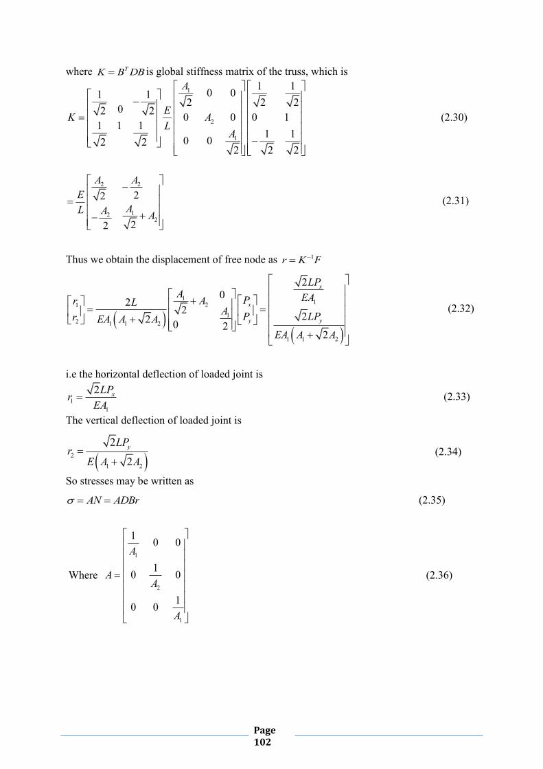
Page 102

where TK B DB is global stiffness matrix of the truss, which is 1

2

1

1 10 01 12 2 202 2 0 0 0 1

1 1 11 10 02 22 22

A

EK AL

A

(2.30)

2 2

122

22

22

A AE

AL A A

(2.31)

Thus we obtain the displacement of free node as 1r K F

1 1211

2 1 1 2

1 1 2

20

22 22 0 2

2

x

x

yy

LPA EAPAr L

A LPPr EA A AEA A A

(2.32)

i.e the horizontal deflection of loaded joint is

11

2 xLPrEA

(2.33)

The vertical deflection of loaded joint is

2

1 2

2

2yLP

rE A A

(2.34)

So stresses may be written as

AN ADBr (2.35)

Where

1

2

1

1 0 0

10 0

10 0

A

AA

A

(2.36)

Page 103

1 1 21 2

11

2 22 1 2

31 2

1 1 2

12 21 1 1 1

2 2 2 2 20 1

21 1 1 12 2 2 2 1

2 2

yx

y

yx

PPA A A

r rPrE E r

rL L A Ar r

PPA A A

(2.37)

The tensile stress of bar 1 is

1

1 1 2

12 2

yx PPA A A

(2.38)

The tensile stress of bar 2 is

2

1 2

2

2yP

A A

(2.39)

The compressive stress of bar 3 is

3

1 1 2

12 2

yx PPA A A

(2.40)

Considering

cosxP P

(2.41)

and sinyP P

(2.42)

Assuming 045 multi-objective structural design problem, the diagram of which is

presented by Fig.-2.2 can be formulated as

(P2.2)

1 2 1 2, 2 2 ;Minimize WT A A L A A (2.43)

1 21 2

,2

PLMinimize A AE A A

(2.44)

such that

1 2

1 1 2 121 1 2

2, ;

2 2T

P A AA A

A A A

(2.45)

2 1 2 21 2

, ;2

TPA AA A

(2.46)

Page 104

23 1 2 32

1 1 2

, ;2 2

CPAA AA A A

(2.47)

min max 1,2i i iA A A i

2.3.3 Design Criteria for Thickness Optimization

The design method of JPCP, presented by Westergaard‟s Analysis, is the background of

current design method of PCA. This method has taken into consideration of fatigue analysis,

deflection analysis for subgrade, corner stress analysis in the following way.

Fatigue Analysis

Fig.-2.3 Typical schematic diagram for fatigue analysis of JPCP

Fatigue analysis of JPCP is well described in Report 1-26 (NCHRP, 1990)[88], where

Damage Ratio DR have been derived considering curling stress ,k sub grade support j

and loading group (i) affixed in Eq.(2.48). However, combined effect of all such factor

initiates crack in the slab (Fig.- 2.3) while the cited ratio is greater than unity.

3, ,

1 1 1 , .

p mi k j

j k i i k j

nDR

N

(2.48)

Where, m is the total number of load groups, p is the number of period in year, , ,i k jn is the

predicted number of load repetitions for the i th load group, k th curling condition and j th

period whereas , ,i k jN is the allowable number of load repetitions for the same condition . By

neglecting the combined effect of warping and curling due to temperature, (2.48) had been

transformed into Eq.(2.49).

1

mi

i i

nDRN

(1.49)

Where DR has been measured by the arithmetic sum of ratio of predicted number of load

repetitions for i th load group in to the allowable number of load repetitions for the i th

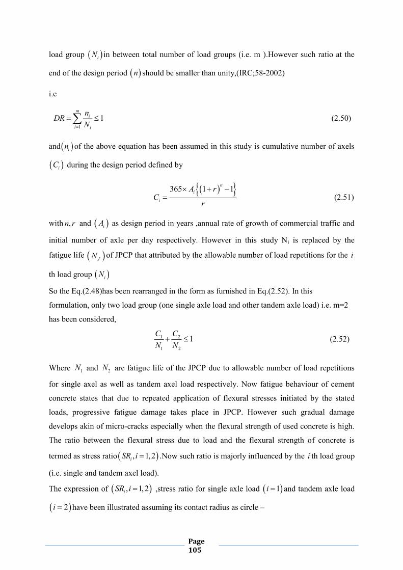
Page 105

load group iN in between total number of load groups (i.e. m ).However such ratio at the

end of the design period n should be smaller than unity,(IRC;58-2002)

i.e

11

mi

i i

nDRN

(2.50)

and in of the above equation has been assumed in this study is cumulative number of axels

iC during the design period defined by

365 1 1ni

i

A rC

r

(2.51)

with ,n r and iA as design period in years ,annual rate of growth of commercial traffic and

initial number of axle per day respectively. However in this study Ni is replaced by the

fatigue life fN of JPCP that attributed by the allowable number of load repetitions for the i

th load group iN

So the Eq.(2.48)has been rearranged in the form as furnished in Eq.(2.52). In this

formulation, only two load group (one single axle load and other tandem axle load) i.e. m=2

has been considered,

1 2

1 2

1C CN N

(2.52)

Where 1N and 2N are fatigue life of the JPCP due to allowable number of load repetitions

for single axel as well as tandem axel load respectively. Now fatigue behaviour of cement

concrete states that due to repeated application of flexural stresses initiated by the stated

loads, progressive fatigue damage takes place in JPCP. However such gradual damage

develops akin of micro-cracks especially when the flexural strength of used concrete is high.

The ratio between the flexural stress due to load and the flexural strength of concrete is

termed as stress ratio , 1,2iSR i .Now such ratio is majorly influenced by the i th load group

(i.e. single and tandem axel load).

The expression of , 1,2iSR i ,stress ratio for single axle load 1i and tandem axle load

2i have been illustrated assuming its contact radius as circle –

Page 106

3

2 4

3 1 1.18 1 24 1ln 1.843 100 3 2

i

if

P aEh v vh ka l

SR hS

for 1,2i (2.53)

Where and E denote Poisson‟s ratio and modulus of elasticity of cement concrete

respectively. , ,l a h and fS denote radius of relative stiffness, radius of load contact areas

thickness of the slab and flexural strength of concrete respectively. The relation between

iN and iSR for single axle load 1i and tandem axle 2i is expressed as per IRC

58- 2002 below-

0.45i iN if SR h (2.54)

3.2684.2577 0.45 0.55

0.4325i ii

N if SR hSR h

(2.55)

0.9718

0.082810 0.55iSR h

i iN if SR h (2.56)

Therefore three cases will come up for consideration to demonstrate the stress ratio in terms

of fatigue life and axel load.

Case I : When Eq.(2.54) is influenced over the Eq.(2.52), the DR remain unchanged as

Eq.(2.54) as the relation is trivially true Case II: When Eq.(2.55) is influenced over the Eq.(2.52) the DR is transforms into

2 3.268 2 6.536 2

1 1 2 1 2 1 2, , , , 365 1 1 0.4325 0.4325 0.5 4.2577nF l h k A A r SR h SR h A A r

(2.57) Case 3: When Eq.(2.56) is influenced over the equation Eq.(2.52), the DR is expressed as

2

1 22 1 2 1 2

365 1 1 0.25, , , , 2 23.47

0.25 0.0828

r SR h SR hF l h k A A Log Log A A

r

(2.58) In the above expression A is initial number of axle per day in year which is not greater than

the sum of initial number of axle per day due to single axle 1A and initial number of axle per

day due to tandem axle 2A .

Deflection Analysis for Subgrade

Page 107

Subgrade strength is expressed in terms of modulus of subgrade (k) that has been measured

as pressure per unit deflection of the cited subgrade. However if the sustained deflection ( i.e.

,SALD k l and ,TALD k l ) are known for different type of vehicular load at JPCP, such

modulus can be represented by Eq.2.59 and Eq.2.60 respectively (Huang, 2004)[50]

112

0.431, 1 0.82SALP aD k l d

kl l

(2.59)

and

222

0.431, 1 0.82TALP aD k l d

kl l

(2.60)

where 1 2,d d are the limiting value of deflection of concrete due to single axle load 1P and

tandem axle load 2P respectively.

Corner Stress Analysis

In the corner region, the temperature stress is negligible but the load stress is maximum at night when the slab corners have a tendency to lift up, due to warping and lose partly its foundation support as the diagram affixed in Fig.- a, Fig.-b, Fig.-c.

Fig.-2.4 Temperature Effect of JPCP in Different Time

Therefore, load stresses (corner stress for single axle, CSALS h ; tandem axle load, C

TALS h ) at

Page 108

corner region may be obtained as per modified Westergaard‟s analysis for different types of load groups as per Eq.(2.61), and Eq.(2.62), respectively.

1.2

12

3 21CSAL f

P aS h Sh l

(2.61)

1.2

22

3 21CTAL f

P aS h Sh l

(2.62)

Formulation for Optimization of Thickness of Rigid Pavement

The first step of formulation of JPCP is to formulate the pavement optimization problem by

defining objective function (minimum thickness) and the constraints (fatigue life consumed,

deflection and corner stress due to single and tandem axle) that control the solution.

Design input parameters

The input parameters that influence the design are Poisson ratio , Load due to single axle

1P , Load due to tandem axle 2P , Modulus of elasticity of concrete E , Modulus of

subgrade reaction k , Radius of load contact areas assumed circular a , Initial number of

axles per day in the year A , Design period in year n , Annual rate of growth of commercial

traffic r , Limiting value of deflection due to single axle 1d , Limiting value of deflection

due to tandem axle 2d , Flexural strength of concrete fS ,

Design method

For determining optimum thickness of JPCP, a crisp mathematical model has been

formulated. Here Thickness of Slab (TS) has been minimized subjected to a specified set of

constraints Eq.(2.62-2.71) .Here the optimum design is

(P2.3)

Minimize TS h h (2.63)

Subject to

2 3.268 2 6.536 2


(2.64)

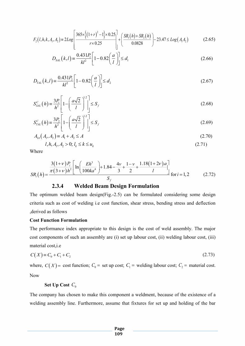
Page 109

2

1 22 1 2 1 2

365 1 1 0.25, , , , 2 23.47

0.25 0.0828


r

(2.65)

112

0.431, 1 0.82SALP aD k l d

kl l

(2.66)

222

0.431, 1 0.82TALP aD k l d

kl l

(2.67)

1.2

12

3 21CSAL f

P aS h Sh l

(2.68)

1.2

22

3 21CTAL f

P aS h Sh l

(2.69)

1 2 1 2,IAA A A A A A (2.70)

1 2, , , 0;l h A A k kl k u (2.71)

Where

3

2 4

3 1 1.18 1 24 1ln 1.843 100 3 2

i

if

P aEh v vh ka l

SR hS

for 1,2i (2.72)

2.3.4 Welded Beam Design Formulation The optimum welded beam design(Fig.-2.5) can be formulated considering some design

criteria such as cost of welding i.e cost function, shear stress, bending stress and deflection

,derived as follows

Cost Function Formulation

The performance index appropriate to this design is the cost of weld assembly. The major

cost components of such an assembly are (i) set up labour cost, (ii) welding labour cost, (iii)

material cost,i.e

0 1 2C X C C C (2.73)

where, C X cost function; 0C set up cost;

1C welding labour cost; 2C material cost.

Now

Set Up Cost 0C

The company has chosen to make this component a weldment, because of the existence of a

welding assembly line. Furthermore, assume that fixtures for set up and holding of the bar

Page 110

during welding are readily available. The cost 0C can therefore be ignored in this particular

total cost model.

Welding Labour Cost 1C

Assume that the welding will be done by machine at a total cost of $10/hr (including

operating and maintenance expense). Furthermore suppose that the machine can lay down a

cubic inch of weld in 6 min. The labour cost is then

1 3 3$ 1 $ min $10 6 1

60 min w wC V Vhr in in

(2.74)

Where wV weld volume,in3

Material Cost 2C

2 3 4w BC C V C V

Where 3C cost per volume per weld material,$/in3 (0.37)(0.283) ; 4C cost per volume

of bar stock,$/in3 (0.37)(0.283) ; BV volume of bar,in3.

From geometry 2wV h l ;volume of the weld material,in3

; 2

1 2weldV x x and BV tb L l

;volume of bar ,in3 3 4 2barV x x L x .

Therefore cost function become

2 2 23 4 1 2 3 4 21.10471 0.04811 14.0C X h l C h l C tb L l x x x x x

(2.75)

Constraints Derivation from Engineering Relationship

Fig.-2.5 Shear Stresses in the Weld Group.

Maximum shear stress in weld group To complete the model it is necessary to define important stress states Direct or primary shear stress i.e

11 22 2

Load P P PThroat area A hl x x

(2.76)

Since the shear stress produced due to turning moment

.M P e at any section, is

proportional to its radial distance from centre of gravity of the joint „G‟, therefore stress due

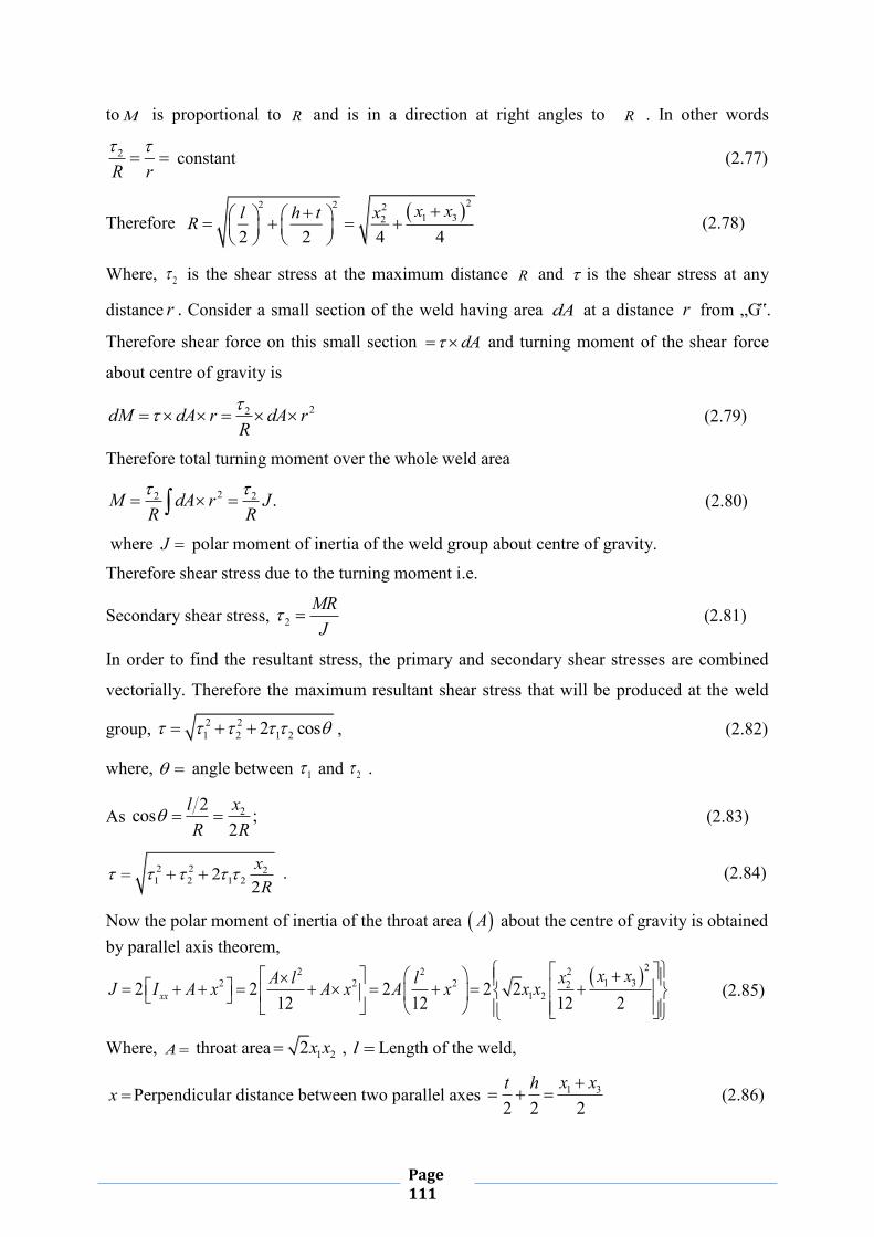
Page 111

to M is proportional to R and is in a direction at right angles to R . In other words

2

R r

constant (2.77)

Therefore 22 2 2

1 32

2 2 4 4x xxl h tR

(2.78)

Where, 2 is the shear stress at the maximum distance R and is the shear stress at any

distance r . Consider a small section of the weld having area dA at a distance r from „G‟.

Therefore shear force on this small section dA and turning moment of the shear force

about centre of gravity is

22dM dA r dA rR

(2.79)

Therefore total turning moment over the whole weld area

22 2 .M dA r JR R

(2.80)

where J polar moment of inertia of the weld group about centre of gravity.

Therefore shear stress due to the turning moment i.e.

Secondary shear stress, 2MRJ

(2.81)

In order to find the resultant stress, the primary and secondary shear stresses are combined

vectorially. Therefore the maximum resultant shear stress that will be produced at the weld

group, 2 21 2 1 22 cos , (2.82)

where, angle between 1 and 2 .

As 22cos ;2xl

R R

(2.83)

2 2 21 2 1 22

2xR

. (2.84)

Now the polar moment of inertia of the throat area A about the centre of gravity is obtained by parallel axis theorem,

222 2

1 32 2 2 21 22 2 2 2 2

12 12 12 2xx

x xxA l lJ I A x A x A x x x

(2.85)

Where, A throat area 1 22x x , l Length of the weld,

x Perpendicular distance between two parallel axes 1 3

2 2 2x xt h

(2.86)

Page 112

Maximum bending stress in beam

Now Maximum bending moment PL , Maximum bending stressTZ

,where ;T PL

Z section modulus ;Iy

I moment of inertia3

;12bt

y distance of extreme fibre from

centre of gravity of cross section ;2t

Therefore 2

6btZ .

So bar bending stress 2 24 3

6 6 .T PL PLxZ bt x x

(2.87)

Maximum deflection in beam

Maximum deflection at cantilever tip 3 3 3 3

3 3 24 3

4 43 3

12

PL PL PL PLxbtEI Ebt Ex xE

(2.88)

Buckling load of beam

Buckling load can be approximated by 24.013 1C

EIC a ElP xl l C

(2.89)

2 6

2

4.01336 1

2 4

t bE t EL L G

6 63 4 3

2

4.013 / 361

2 4EGx x x EL L G

(2.90)

where, I moment of inertia3

;12bt

torsional rigidity 31 ;3

C GJ tb G ; .2tl L a

Crisp Formulation of Welded Beam Design In design formulation a welded beam (Fig. -2.6) has to be designed at minimum cost whose constraints are shear stress in weld ,bending stress in the beam ,buckling load on the

bar P ,and deflection of the beam .The design variables are

1

2

3

4

x hx lx tx b

where h is the

weld size, l is the length of the weld , t is the depth of the welded beam, b is the width of the welded beam.

Page 113

Fig.-2.6 Design of the welded beam

The single-objective crisp welded beam optimization problem can be formulated as follows (P2.4)

21 2 2 3 41.10471 0.04811 14Minimize C X x x x x x (2.91)

such that

1 max 0g x x

(2.92)

2 max 0g x x

(2.93)

3 1 4 0g x x x

(2.94)

24 1 2 3 4 20.10471 0.04811 14 5 0g x x x x x x

(2.95)

5 10.125 0g x x

(2.96)

6 max 0g x x

(2.97)

7 0Cg x P P x

(2.98)

1 2 3 4, , , 0,1x x x x

(2.99)

where 2 221 1 2 22

2xxR

; 11 22

Px x

; 2MRJ

; 2

2xM P L

;

221 32

4 2x xxR

;

221 31 2 2 ;

12 22x xx x xJ

24 3

6 ;PLxx x

3

24 3

4 ;PLxEx x

6 63 4 3

2

4.013 / 361

2 4C

EGx x x EP xL L G

as derived as Eq.(2.82), Eq.(2.76), Eq.(2.81),

Eq.(2.80), Eq. (2.78), Eq. (2.85), Eq. (2.87), Eq. (2.88), Eq. (2.90), respectively. Again P

Force on beam ; L Beam length beyond weld; 1x Height of the welded beam; 2x Length

of the welded beam; 3x Depth of the welded beam; 4x Width of the welded beam;

x Design shear stress; x Design normal stress for beam material; M Moment of

Page 114

P about the centre of gravity of the weld , J Polar moment of inertia of weld group; G

Shearing modulus of Beam Material; E Young modulus; max Design Stress of the weld;

max Design normal stress for the beam material; max Maximum deflection; 1

Primary stress on weld throat. 2 Secondary torsional stress on weld.

Page 115

CHAPTER 3

Truss Design Optimization using Neutrosophic Optimization

Technique: A Comparative Study

The research area of optimal structural design has been receiving increasing attention from

both academia and industry over the past four decades in order to improve structural

performance and to reduce design costs. However, in the real world, uncertainty or vagueness

is prevalent in the Engineering Computations. In the context of structural design the

uncertainty is connected with lack of accurate data of design factors. This problem has been

solving by use of fuzzy mathematical algorithm for dealing with this class of problems.

Fuzzy set (FS) theory has long been introduced to deal with inexact and imprecise resources

by Zadeh [133], as an application, Bellman and Zadeh [10] used the FS theory to the decision

making problem. In such extension, Atanassov [1] introduced Intuitionistic Fuzzy set (IFS)

which is one of the generalizations of FS theory and is characterized by a membership

function, a non membership function and a hesitancy function. In FS the degree of acceptance

is only considered but IFS is characterized by a degree of acceptance and degree of rejection

so that their sum is less than one. As a generalization of FS and IFS, F. Smrandache [94]

introduced a new notion which is known as neutrosophic set (NS in short) in 1995.NS is

characterized by degree of truth membership, degree of indeterminacy membership and

degree of falsity membership. The concept of NS generates the theory of neutrosophic sets by

expressing indeterminacy of imprecise information. This theory is considered as complete

representation of structural design problems like other decision making problems. Therefore,

if uncertainty is involved in a structural model, we use fuzzy theory while dealing

indeterminacy, we need neutrosophic theory .This is the first time NSO technique is applied

in structural design. Several researchers like Wang et al. [119] first applied α-cut method to

structural designs where the non-linear problems were solved with various design levels α,

and then a sequence of solutions were obtained by setting different level-cut value of α. To

design a four–bar mechanism for function generating problem, Rao [89] used the same α-cut

method.

Page 116

Structural optimization with fuzzy parameters was developed by Yeh et al. [131]. Xu [13]

used two-phase method for Fuzzy Optimization (FO) of structures. A level-cut of the first and

second kind approach used by Shih et al. [95] for structural design optimization problems

with fuzzy resources. Shih et al. [96] developed alternative α-level-cuts methods for optimum

structural design with fuzzy resources. Dey et al. [32] used generalized fuzzy number in

context of a structural design. Dey et al. [33] developed parameterized t-norm based FO

method for optimum structural design. Also, a parametric geometric programming is

introduced by Dey et.al [34] to Optimize shape design of structural model with imprecise

coefficient. A transportation model was solved by Jana et al.[57] using multi-objective

intuitionistic fuzzy linear programming. Dey et al. [35] solved two bar truss non linear

problem by using Intuitionistic Fuzzy Optimization (IFO) problem. Dey et al. [36] used IFO

technique for multi objective optimum structural design. R-x Liang et al.[66] applied

interdependent inputs of single valued trapezoidal neutrosophic information on Multi-criteria

group decision making problem. P Ji et al. [58], S Yu et al. [132] did so many research study

on application based neutosophic sets and intuitionistic linguistic number . Z-p Tian et

al.[115] Simplified neutrosophic linguistic multi-criteria group decision-making approach to

green product development. Again J-j Peng et al.[81] introduced multi-valued neutrosophic

qualitative flexible approach based on likelihood for multi-criteria decision-making

problems.Also H Zhang et al [135] investigates a case study on a novel decision support

model for satisfactory restaurants utilizing social information. P Ji et al. [58] developed a

projection-based TODIM method under multi-valued neutrosophic environments and its

application in personnel selection.

The present study investigates computational algorithm for solving single-objective structural

problem by single valued Neutrosophic Optimization (NSO) approach. The impact of linear

and nonlinear truth, indeterminacy and falsity membership functions in such optimization

process also has been studied here. A comparison is made numerically among FO, IFO and

NSO technique. From our numerical result, it is clear that NSO technique provides better

results than FO as well as IFO.

3.1 General Formulation of Single-objective Structural Model

In sizing optimization problems, the aim is to minimize single objective function, usually the

weight of the structure under certain behavioural constraints which are displacement or

stresses. The design variables are most frequently chosen to be dimensions of the cross

Page 117

sectional areas of the members of the structures. Due to fabrications limitations the design

variables are not continuous but discrete for belongingness of cross-sections to a certain set.

A discrete structural optimization problem can be formulated in the following form

(P3.1)

Minimize WT A (3.1)

, 1,2,...,i isubject to A A i m (3.2)

, 1,2,...,djA R j n

(3.3)

where WT A represents objective function, i A is the behavioural constraints and

i A denotes the maximum allowable value , m and n are the number of constraints and

design variables respectively. A given set of discrete value is expressed by dR and in this

paper objective function is taken as

1

m

i i ii

WT A l A

(3.4)

and constraint are chosen to be stress of structures as follows

i iA with allowable tolerance 0i for 1,2,....,i m (3.5)

Where i and il are weight of unit volume and length of thi element respectively, m is the

number of structural element, i and 0i are the thi stress , allowable stress respectively

3.2 Neutrosophic Optimization Technique to Solve Single-objective

Structural Optimization Problem (SOSOP)

To solve the SOSOP (P3.1), step 1 of 1.29 is used and we will get optimum solutions of two

sub problem as 1A and 2A .After that according to step 2 we find upper and lower bound of

membership function of objective function as , ,T I FWT A WT A WT AU U U and , ,T I F

WT A WT A WT AL L L

where 1 2max , ,T

WT AU WT A WT A

(3.6)

1 2min , ,TWT AL WT A WT A

(3.7)


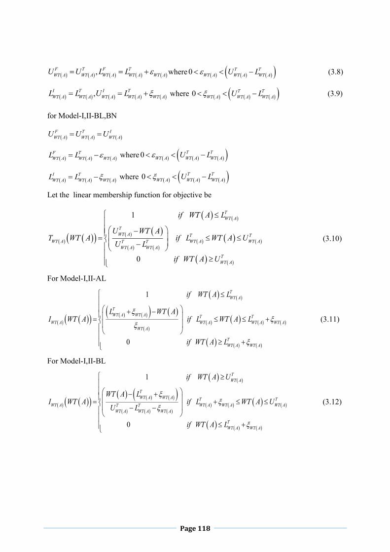
Page 118

,F T F TWT A WT A WT A WT A WT AU U L L where 0 T T

WT A WT A WT AU L

(3.8)

,I T I TWT A WT A WT A WT A WT AL L U L where 0 T T

WT A WT A WT AU L

(3.9)


F T I

WT A WT A WT AU U U

F TWT A WT A WT AL L where 0 T T

WT A WT A WT AU L

I TWT A WT A WT AL L where 0 T T

WT A WT A WT AU L

Let the linear membership function for objective be

1

0

TWT A

TWT A T T

WT A WT A WT AT TWT A WT A

TWT A

if WT A L

U WT AT WT A if L WT A U

U L

if WT A U

(3.10)

For Model-I,II-AL

1

0

TWT A

TWT A WT A T T

WT A WT A WT A WT AWT A

TWT A WT A

if WT A L

L WT AI WT A if L WT A L

if WT A L

(3.11)

For Model-I,II-BL

1

0

TWT A

TWT A WT A T T

WT A WT A WT A WT AT TWT A WT A WT A

TWT A WT A

if WT A U

WT A LI WT A if L WT A U

U L

if WT A L

(3.12)

Page 119

0

1

TWT A WT A

TWT A WT A T T

WT A WT A WT A WT AT TWT A WT A WT A

TWT A

if WT A L

WT A LF WT A if L WT A U

U L

if WT A U

(3.13)

and constraints be

1

0

i

i

i ii

i i

i

Ti

Ti T T

i iA T T

Ti

if A L

U AT A if L A U

U L

if A U

(3.14)

For Model-I,II-AL

1

0

i

i xi

i ii i

i

i i

Ti

Ti T T

i iA xx

Ti x

if A L

L AI A if L A L

if A L

(3.15)

For Model-I,II-BL

1

0

i

i xi

i ii i

i i i

i i

Ti

Ti T T

i iA xT Tx

Ti x

if A U

A LI A if L A U

U L

if A L

(3.16)

0

1

i i

i i

i ii i

i i i

i

Ti x

Ti x T T

i iA xT Tx

Ti

if A L

A LF A if L A U

U L

if A U

(3.17)

where for 01,2,..., 0 ,

i i ix Aj m

and if non-linear membership function be considered for objective function WT A then

Page 120

1

1 exp

0

TWT A

TWT A T T


TWT A

if WT A L


U L

if WT A U

(3.18)

For Model-I,II-AN

1

exp

0

TWT A

TWTWT A T T

WTWT A WT A WT AWT

TWTWT A

if WT A L


if WT A L

(3.19)

For Model-I,II-BN

1

exp

0

TWT A

TWTWT A T T

WTWT A WT A WT AT TWTWT A WT A

TWTWT A

if WT A U


U L

if WT A L

(3.20)

0

1 1 tanh2 2 2

1

TWTWT A

T TWTWT A WT A T T

WT WTWT A WT A WT A

TWT A

if WT A L

U LF WT A WT A if L WT A U

if WT A U

(3.21)

0 , T TWT WT WT WTwhere U L and if nonlinear truth, indeterminacy and falsity

membership functions be considered for constraints then

1

1 exp

0

i

i

i ii

i i

i

Ti

TT T

i iA T T

Ti

if A L

U AT A if L A U

U L

if A U

(3.22)

For Model-I,II-AN

Page 121

1

exp

0

i

i i

i i ii

i

i i

Ti

Ti T T

i iA

Ti

if A L

L AI A if L A L

if A L

(3.23)

For Model-I,II-BN

1

exp

0

i

i i

i i ii

i i i

i i

Ti

Ti T T

i iA T T

Ti

if A U

A LI A if L A U

U L

if A L

(3.24)

0

1 1 tanh2 2 2

1

i i

i i i

i i i ii

i

Ti

T TT T

i i iA

Ti

if A L

U LF A A if L A U

if A U

(3.25)

where , are non-zero parameters prescribed by the decision maker.

0 ,i i i i

T Twhere U L

then according to Smarandache’s definition of intersection of Neutrosophic sets and

decision making criteria the neutrosophic optimization problem can be formulated as

(P3.2)

Model-I- AL, BL, AN, BN

Maximize

(3.26)

such that

;WT AT WT A

(3.27)

;

i iAT A

(3.28)

;WT A

I WT A

(3.29)

;

i iAI A

(3.30)

;WT A

F WT A

(3.31)

i iAF A

(3.32)

Page 122

;i ix

(3.33)

3; ; ; (3.34)

, , 0,1

(3.35)

Where Model-I-AL,AN and Model-I-BL,BN stand for the neutrosophic optimization

algorithm with indeterminacy membership function as of decreasing sense and as of

increasing sense respectively.

But in real life problem decision maker needs to minimize indeterminacy membership

function. So nutrosophic optimization problem also can be formulated as

(P3.3)

Model-II-AL,AN,BL,BN

Maximize

(3.36)

such that

;WT AT WT A

(3.37)

;

i iAT A

(3.38)

;WT A

I WT A

(3.39)

;

i iAI A

(3.40)

;WT A

F WT A

(3.41)

i iAF A

(3.42)

;i ix

(3.43)

3; ; ; (3.44)

, , 0,1

Where Model-II-AL,AN and Model-II-BL,BN stand for the neutrosophic optimization

algorithm with indeterminacy membership function considered as of decreasing sense and as

of increasing sense respectively.

Now the above problem can be simplified to following crisp linear programming problem,

whenever linear membership are considered, as

(P3.4)

Model-I-AL

Page 123

Maximize (3.45)

Such that

;T T TWT A WT A WT AWT A U L U

(3.46)

;T

WT A WT A WT AWT A L

(3.47)

;T T TWT A WT A WT A WT A WT AWT A U L L

(3.48)

;T T T

T T TT A A AA U L U

(3.49)

;T T T

TT A A AA L

(3.50)

;T T T T T

T T TT A A A A AA U L L

(3.51)

;C C C

T T TC A A AA U L U

(3.52)

;C C C

TC A A AA U

(3.53)

3; (3.54)

; ; (3.55)

, , 0,1

(3.56)

(P3.5)

Model-I-BL

Maximize (3.57)

Such that


(3.58)


(3.59)


(3.60)

;T T T

T T TT A A AA U L U

(3.61)

;T T T T T


(3.62)

;T T T T T


(3.63)

Page 124

;C C C

T T TC A A AA U L U

(3.64)

;C C C C C

T T TC A A A A AA U L L

(3.65)

3; (3.66)

; ; (3.67)

, , 0,1

(3.68)

and crisp linear programming problem like Model-I-A whenever non-linear membership

function is considered as

(P3.6)

Model-I-AN

Maximize (3.69)

such that

;

T TWT A WT A T

WT A

U LWT A U

(3.70)

;2

T TWT A WT A WT A

WT A

U LWT A

(3.71)

;T


(3.72)

;i i

i

T TT

i

U LA U

(3.73)

;

ii i

Ti A AA L

(3.74)

;2

i i i

i

T TA

iA

U LA

(3.75)

3; (3.76)

; ; (3.77)

, , 0,1

(3.78)

Where ln 1 ;

(3.79)

4; (3.80)

6 ;WT A F F

WT A WT AU L

(3.81)

Page 125

ln ; (3.82)

1tanh 2 1 .

(3.83)

6 ;

i

i i

A F FA A

andU L

(3.84)

(P3.7)

Model-I-BN

Maximize (3.85)

such that

;

T TWT A WT A T

WT A

U LWT A U

(3.86)

;2

T TWT A WT A WT A

WT A

U LWT A

(3.87)

;T T T

WT A WT A WT A WT A WT AWT A U L L

(3.88)

;i i

i

T TT

i

U LA U

(3.89)

;

i i ii i

T T Ti A AA U L L

(3.90)

;2

i i i

i

T TA

iA

L UA

(3.91)

3; (3.92)

; ; (3.93)

, , 0,1

(3.94)

Where ln 1 ;

(3.95)

4; (3.96)

6 ;WT A F F

WT A WT AU L

(3.97)

ln ; (3.98)

1tanh 2 1 .

(3.99)

Page 126

6 ;

i

i i

A F FA A

andU L

(3.100)

.

Using linear and nonlinear truth, indeterminacy, and falsity membership function Model-II

can be simplified as

(P3.8)

Model-II-AL

Maximize (3.101)

Such that


(3.102)

;T


(3.103)


(3.104)

;T T T

T T TT A A AA U L U

(3.105)

;T T T

TT A A AA L

(3.106)

;T T T T T


(3.107)

;C C C

T T TC A A AA U L U

(3.108)

;C C C

TC A A AA U

(3.109)

3; (3.110)

; ; (3.111)

, , 0,1

(3.112)

(P3.9)

Model-II-BL

Maximize (3.113)

Such that


(3.114)

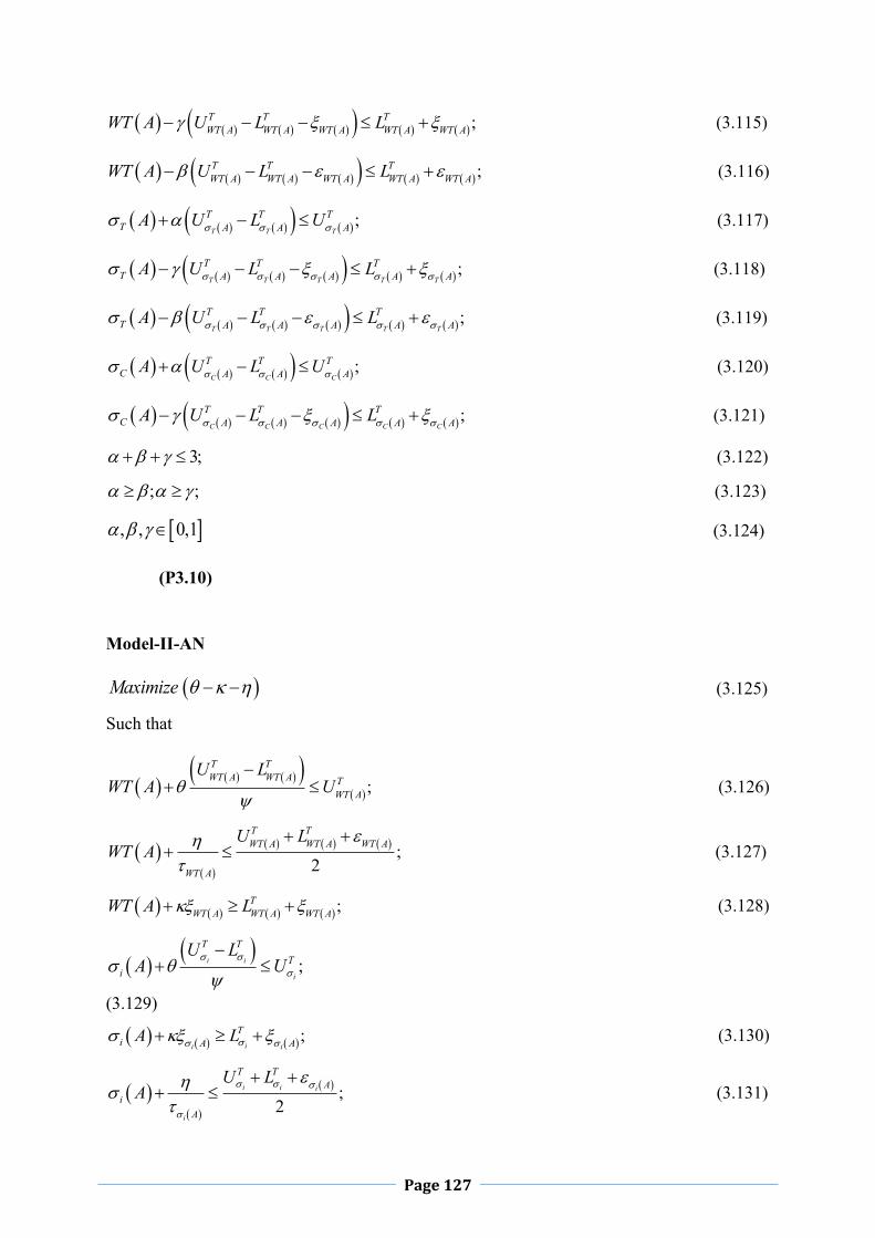
Page 127


(3.115)


(3.116)

;T T T

T T TT A A AA U L U

(3.117)

;T T T T T


(3.118)

;T T T T T


(3.119)

;C C C

T T TC A A AA U L U

(3.120)

;C C C C C

T T TC A A A A AA U L L

(3.121)

3; (3.122)

; ; (3.123)

, , 0,1

(3.124)

(P3.10)

Model-II-AN

Maximize (3.125)

Such that

;

T TWT A WT A T

WT A

U LWT A U

(3.126)

;2

T TWT A WT A WT A

WT A

U LWT A

(3.127)

;T


(3.128)

;i i

i

T TT

i

U LA U

(3.129)

;ii i

Ti A AA L

(3.130)

;2

i i i

i

T TA

iA

U LA

(3.131)

Page 128

3; (3.132)

; ; (3.133)

, , 0,1

(3.134)

Where ln 1 ;

(3.135)

4; (3.136)

6 ;WT A F F

WT A WT AU L

(3.137)

ln ; (3.138)

1tanh 2 1 .

(3.139)

6 ;

i

i i

A F FA A

andU L

(3.140)

(P3.11)

Model-II-BN

Maximize (3.141)

such that

;

T TWT A WT A T

WT A

U LWT A U

(3.142)

;2

T TWT A WT A WT A

WT A

U LWT A

(3.143)

;T T T


(3.144)

;i i

i

T TT

i

U LA U

(3.145)

;i i ii i

T T Ti A AA U L L

(3.146)

;2

i i i

i

T TA

iA

L UA

(3.147)

3; (3.148)

; ; (3.149)

Page 129

, , 0,1

(3.150)

Where ln 1 ;

(3.151)

4; (3.152)

6 ;WT A F F

WT A WT AU L

(3.153)

ln ; (3.154)

1tanh 2 1 .

(3.155)

6 ;

i

i i

A F FA A

andU L

(3.156)

All these crisp nonlinear programming problem can be solved by appropriate mathematical

algorithm.

3.3 Numerical Solution of Two Bar Truss Design using Single

Objective NSO Technique

A well-known two-bar planar truss structure (Fig.-3.1)is considered and the detail

formulation is given in appendix. The design objective is to minimize weight of the structural

1 2, , BWT A A y of a statistically loaded two-bar truss subjected to stress 1 2, ,i BA A y

constraints on each of the truss members 1,2i .

Fig.-3.1 Design of the Two-Bar Truss(http://www.sciencedirect.com,accessed on 17June

2017)


Page 130

(P3.12)

22 2 21 2 1 2, , B B B B BMinimize WT A A y A x l y A x y (3.157)

Such that

22

AB 1 21

, , ;B B TB AB

P x l yA A y

lA

(3.158)

2 2

BC 1 22

, , ;B B CB BC

P x yA A y

lA

(3.159)

0.5 1.5By

(3.160)

1 20, 0;A A

(3.161)

where P nodal load ; volume density ; l length of AC ; Bx perpendicular distance

from AC to point B . 1A Cross section of bar- AB ; 2A Cross section of bar- BC . T

maximum allowable tensile stress, C maximum allowable compressive stress and

By y -co-ordinate of node B .Input data are given in Table 3.1.

Table 3.1 Input Data for Crisp Model (P3.8)

Applied

load P

KN

Volume

density

3/KN m

Length

l m

Maximum

allowable

tensile

stress T Mpa

Maximum

allowable

compressive

stress C Mpa

Distance of

Bx from

AC

m

100 7.7 2

130

with fuzzy

region

20

90

with fuzzy

region

10

1

Solution: According to step 2 of 1.29,we find upper and lower bound of membership

function of objective function as , ,T I FWT A WT A WT AU U U and , ,T I F

WT A WT A WT AU U U where

14.23932 , 12.57667 ,T F T IWT A WT A WT A WT AU U L L 12.57667F

WT A WT AL with

0 1.66265;WT A and I T

WT A WT A WT AU L where 0 1.66265WT A

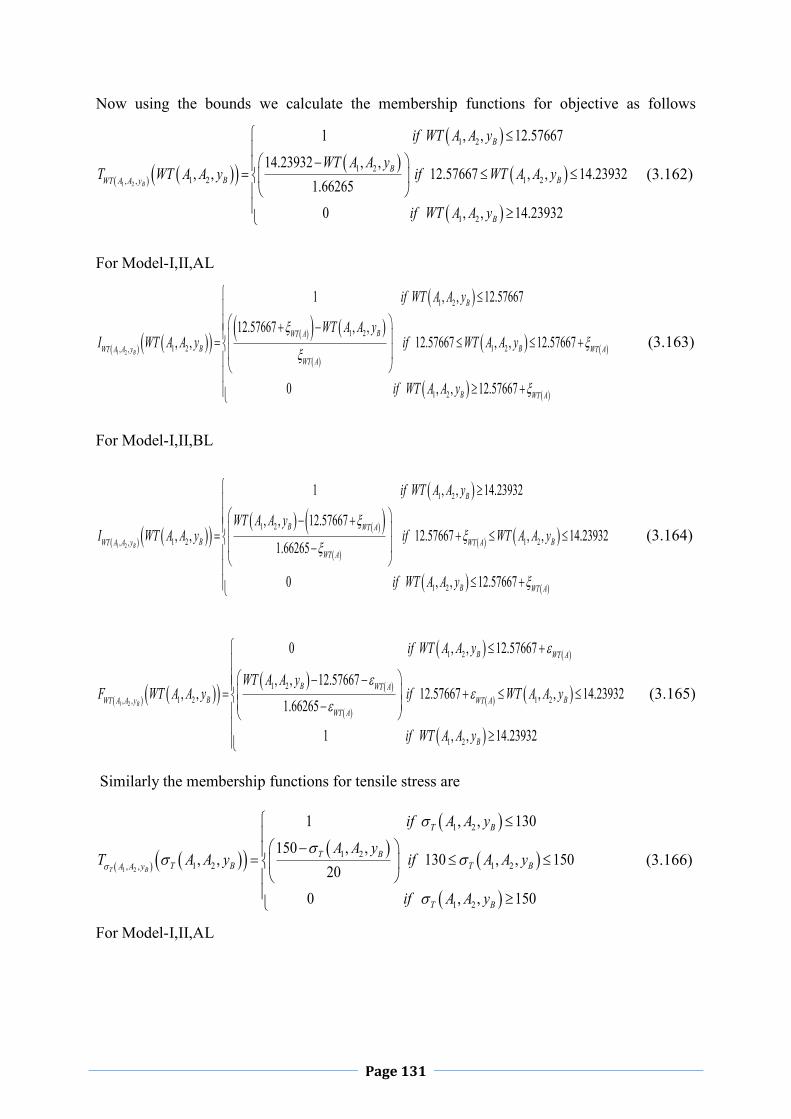
Page 131

Now using the bounds we calculate the membership functions for objective as follows

1 2

1 2

1 21 2 1 2, ,

1 2

1 , , 12.57667

14.23932 , ,, , 12.57667 , , 14.23932

1.662650 , , 14.23932

B

B

BB BWT A A y

B

if WT A A y

WT A A yT WT A A y if WT A A y

if WT A A y

(3.162)

For Model-I,II,AL

1 2

1 2

1 21 2 1 2, ,

1 2

1 , , 12.57667

12.57667 , ,, , 12.57667 , , 12.57667

0 , , 12.57667

B

B

BWT AB BWT A A y WT A

WT A

B WT A

if WT A A y

WT A A yI WT A A y if WT A A y

if WT A A y

(3.163)

For Model-I,II,BL

1 2

1 2

1 21 2 1 2, ,

1 2

1 , , 14.23932

, , 12.57667, , 12.57667 , , 14.23932

1.66265

0 , , 12.57667

B

B

B WT AB BWT A A y WT A

WT A

B WT A

if WT A A y


if WT A A y

(3.164)

1 2

1 2

1 21 2 1 2, ,

1 2

0 , , 12.57667

, , 12.57667, , 12.57667 , , 14.23932

1.66265

1 , , 14.23932

B

B WT A

B WT AB BWT A A y WT A

WT A

B

if WT A A y

WT A A yF WT A A y if WT A A y

if WT A A y

(3.165)

Similarly the membership functions for tensile stress are

1 2

1 2

1 21 2 1 2, ,

1 2

1 , , 130

150 , ,, , 130 , , 150

200 , , 150

T B

T B

T BT B T BA A y

T B

if A A y

A A yT A A y if A A y

if A A y

(3.166)

For Model-I,II,AL

Page 132

1 2

1 2

1 21 2 1 2, ,

1 2

1 , , 130

130 , ,, , 130 , , 130

0 , , 130

T

TT B

T

T

T B

T BT B T BA A y

T B

if A A y

A A yI A A y if A A y

if A A y

(3.167)

For Model-I,II,BL

1 2

1 2

1 21 2 1 2, ,

1 2

1 , , 150

, , 130, , 130 , , 150

20

0 , , 130

T

TT B

T

T

T B

T BT B T BA A y

T B

if A A y


if A A y

(3.168)

1 2

1 2

1 21 2 1 2, ,

1 2

0 , , 130

, , 130, , 130 , , 150

20

1 , , 150

T

T

TT B

T

T B

T BT B T BA A y

T B

if A A y

A A yF A A y if A A y

if A A y

(3.169)

0 , 20T T

where

and the membership functions for compressive stress constraint are

1 2

1 2

1 21 2 1 2, ,

1 2

1 , , 90

100 , ,, , 90 , , 100

100 , , 100

C B

C B

C BC B C BA A y

C B

if A A y


if A A y

(3.170)

For Model-I,II,AL

1 2

1 2

1 21 2 1 2, ,

1 2

1 , , 90

90 , ,, , 90 , , 90

0 , , 90

C

CC B

C

C

C B

C BC B C BA A y

C B

if A A y


if A A y

(3.171)

For Model-I,II,BL

Page 133

1 2

1 2

1 21 2 1 2, ,

1 2

1 , , 100

, , 90, , 90 , , 100

10

0 , , 90

C

CC B

C

C

C B

C BC B C BA A y

C B

if A A y


if A A y

(3.172)

1 2

1 2

1 21 2 1 2, ,

1 2

0 , , 90

, , 90, , 90 , , 100

10

1 , , 100

C

C

CC B

C

C B

C BC B C BA A y

C B

if A A y

A A yF A A y if A A y

if A A y

(3.173)

0 , 10C C

where

Again the nonlinear truth, indeterminacy and falsity membership functions for objectives and

constraints can be formulated as

1 2

1 2

1 21 2 1 2, ,

1 2

1 , , 12.57667

14.23932 , ,, , 1 exp 4 12.57667 , , 14.23932

1.66265

0 , , 14.23932

B

B

BB BWT A A y

B

if WT A A y

WT A A yT WT A A y if WT A A y

if WT A A y

(3.174)

For Model-I,II,AN

1 2

1 2

1 21 2 1 2, ,

1 2

1 , , 12.57667

12.57667 , ,, , exp 12.57667 , , 12.57667

0 , , 12.57667

B

B

WT BB B WTWT A A y

WT

B WT

if WT A A y


if WT A A y

(3.175)

For Model-I,II,BN

1 2

1 2

1 21 2 1 2, ,

1 2

1 , , 14.23932

, , 12.57667, , exp 12.57667 , , 14.23932

1.662650 , , 12.57667

B

B

B WTB WT BWT A A y

WT

B WT

if WT A A y


if WT A A y

(3.176)

1 2

1 2

1 2 1 2 1 2, ,

1 2

0 , , 12.57667

26.815991 1 6, , tanh , , 12.57667 , , 14.239322 2 2 1.66265

1 , , 14.23932

B

B WT

WTB B WT BWT A A y

WT

B

if WT A A y

F WT A A y WT A A y if WT A A y

if WT A A y

(3.177)

Similarly the membership functions for tensile stress are

Page 134

1 2

1 2

1 21 2 1 2, ,

1 2

1 , , 130

150 , ,, , 1 exp 4 130 , , 150

20

0 , , 150

T B

T B

T BT B T BA A y

T B

if A A y


if A A y

(3.178)

For Model-I,II,AN

1 2

1 2

1 21 2 1 2, ,

1 2

1 , , 130

130 ,, , exp 130 , , 130

0 , , 130

T

TT B

T

T

T B

T BT B T BA A y

T B

if A A y


if A A y

(3.179)

For Model-I,II,BN

1 2

1 2

1 21 2 1 2, ,

1 2

1 , , 150

, 130, , exp 130 , , 150

20

0 , , 130

T

TT B

T

T

T B

T BT B T BA A y

T B

if A A y


if A A y

(3.180)

1 2

1 2

1 2 1 2 1 2, ,

1 2

0 , , 130

2801 1 6, , tanh , , 130 , , 1502 2 2 20

1 , , 150

T

T

TT B

T

T B

T B T B T BA A y

T B

if A A y

F A A y A A y if A A y

if A A y

(3.181)

0 , 20T T

where and the membership functions for compressive stress constraint are

1 2

1 2

1 21 2 1 2, ,

1 2

1 , , 90

100 , ,, , 1 exp 4 90 , , 100

10

0 , , 100

C B

C B

C BC B C BA A y

C B

if A A y


if A A y

(3.182)

For Model-I,II,AN

1 2

1 2

1 21 2 1 2, ,

1 2

1 , , 90

90 , ,, , exp 90 , , 90

0 , , 90

C

CC B

C

C

C B

C BC B C BA A y

C B

if A A y


if A A y

(3.183)

Page 135

For Model-I,II,BN

1 2

1 2

1 21 2 1 2, ,

1 2

1 , , 100

, , 90, , exp 90 , , 100

10

0 , , 90

C

CC B

C

C

C B

C BC B C BA A y

C B

if A A y


if A A y

(3.184)

1 2

1 2

1 2 1 2 1 2, ,

1 2

0 , , 90

1901 1 6, , tanh , , 90 , , 1002 2 2 10

1 , , 100

C

C

CC B

C

C B

C B C B C BA A y

C B

if A A y

F A A y A A y if A A y

if A A y

(3.185)

0 , 10C C

where

Now , using above mentioned truth, indeterminacy and falsity linear and nonlinear

membership function NLP (P3.12) can be solved for Model-I-AL,AN, Model-I-BL,BN,

Model-II-AL,AN, Model-II-BL,BN by NSO technique for different values of , ,T CWT

and , ,T CWT . The optimum solution of SOSOP(P3.12) is given in Table 3.2and Table 3.3

and the solution is compared with fuzzy and intuitionistic fuzzy problem.

Table 3.2 Comparison of Optimal Solution of SOSOP (P3.12) for Model I based on Different Methods

Methods

Model

1

2

A

m

2

2

A

m

1 2,WT A A

KN

Bym

Fuzzy single-objective non-

linear programming

(FSONLP)

I-AL .5883491 .7183381 14.23932 1.013955

I-AN .5883491

.7183381

14.23932

1.013955

Intuitionistic

Fuzzy single-

objective non-

linear

programming

(FSONLP)

I-AL

0.33253,WT 4,T

2C

0.5482919 0.6692795 13.19429 0.8067448

I-AN

0.8,WT 16,T

8C

0.6064095 0.6053373 13.59182 0.5211994

Neutosophic

optimization(NSO)

I-AL

0.33253, 4, 2T CWT

.498795, 6, 3T CWT

.5954331 .7178116 13.07546 .818181

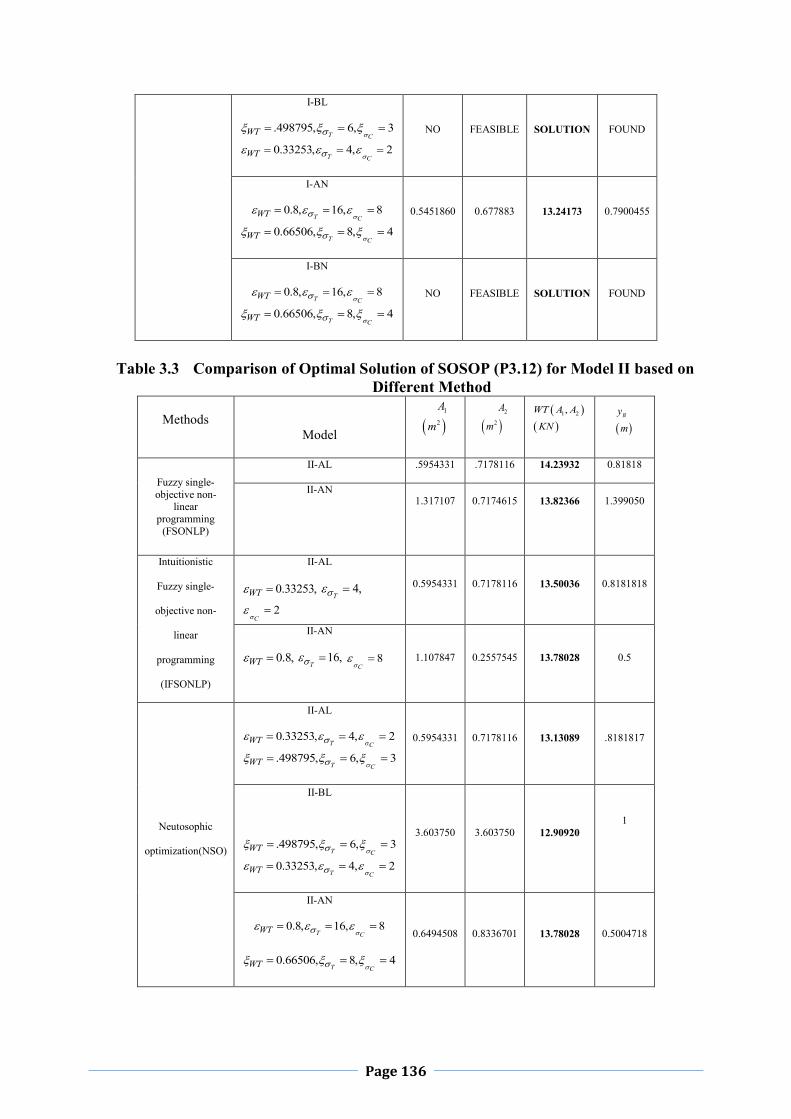
Page 136

I-BL

.498795, 6, 3T CWT

0.33253, 4, 2T CWT

NO FEASIBLE SOLUTION FOUND

I-AN

0.8, 16, 8T CWT

0.66506, 8, 4T CWT

0.5451860 0.677883 13.24173 0.7900455

I-BN

0.8, 16, 8T CWT

0.66506, 8, 4T CWT

NO FEASIBLE SOLUTION FOUND

Table 3.3 Comparison of Optimal Solution of SOSOP (P3.12) for Model II based on

Different Method

Methods

Model

1

2

A

m

2

2

A

m

1 2,WT A A

KN

Bym


linear programming

(FSONLP)

II-AL .5954331 .7178116 14.23932 0.81818

II-AN 1.317107

0.7174615

13.82366

1.399050

Intuitionistic

Fuzzy single-

objective non-

linear

programming

(IFSONLP)

II-AL

0.33253,WT 4,T

2C

0.5954331 0.7178116 13.50036 0.8181818

II-AN

0.8,WT 16,T

8C

1.107847 0.2557545 13.78028 0.5

Neutosophic

optimization(NSO)

II-AL

0.33253, 4, 2T CWT

.498795, 6, 3T CWT

0.5954331 0.7178116 13.13089 .8181817

II-BL

.498795, 6, 3T CWT

0.33253, 4, 2T CWT

3.603750 3.603750 12.90920 1

II-AN

0.8, 16, 8T CWT

0.66506, 8, 4T CWT

0.6494508 0.8336701 13.78028 0.5004718

Page 137

II-BN

0.8, 16, 8T CWT

0.66506, 8, 4T CWT

3.603750 4.043915 13.07546 0.5

Here we get best solutions for the different tolerance ,T CWT and

for indeterminacy

membership function of objective functions whenever indeterminacy is tried to be minimized

(i.e in Model II) for this structural optimization problem. From Table 3.2andTable 3.3, it is

shown that NSO technique gives better optimal result in the perspective of Structural

Optimization.

3.4 Conclusion

This work is done for illustration of NSO technique that using linear and nonlinear

membership function how it can be utilized to solve a single objective-nonlinear structural

problem. The concept of NSO technique allows one to define a degree of truth membership,

which is not a complement of degree of falsity; rather, they are independent with degree of

indeterminacy. The numerical illustration shows the superiority of NSO over FO and IFO.

The results of this study may lead to the development of effective neutrosophic technique for

solving other models in form of single objective nonlinear programming problem in other

field of engineering .

Page 138

CHAPTER 4

Multi-objective Neutrosophic Optimization Technique and its Application to Structural Design

In the field of civil engineering nonlinear structural design optimizations are of great of

importance. So the description of structural geometry and mechanical properties like stiffness

are required for a structural system. However the system description and system inputs may

not be exact due to human errors or some unexpected situations. At this juncture fuzzy set

theory provides a method which deal with ambiguous situations like vague parameters, non-

exact objective and constraint. In structural engineering design problems, the input data and

parameters are often fuzzy/imprecise with nonlinear characteristics that necessitate the

development of fuzzy optimum structural design method. Fuzzy set (FS) theory has long been

introduced to handle inexact and imprecise data by Zadeh [133], Later on Bellman and Zadeh

[10] used the FS theory to the decision making problem. The FS theory also found

application in structural design. Several researchers like Wang et al. [121] first applied α-cut

method to structural designs where the non-linear problems were solved with various design

levels α, and then a sequence of solutions were obtained by setting different level-cut value of

α. Rao [89] applied the same α-cut method to design a four–bar mechanism for function

generating problem. Structural optimization with fuzzy parameters was developed by Yeh et

al. [131]. Xu [13] used two-phase method for fuzzy optimization of structures. Shih et al. [96]

used level-cut approach of the first and second kind for structural design optimization

problems with fuzzy resources. Shih et al. [95] developed alternative α-level-cuts methods for

optimum structural design with fuzzy resources. Dey et al. [35] used generalized fuzzy

number in context of a structural design. Dey et al.[33]used basic t-norm based fuzzy

optimization technique for optimization of structure.

In such extension, Atanassov [1] introduced Intuitionistic Fuzzy Set (IFS) which is one of the

generalizations of fuzzy set theory and is characterized by a membership function, a non-

membership function and a hesitancy function. In FS the degree of acceptance is only

considered but IFS is characterized by a membership function and a non-membership

function so that the sum of both values is less than one. A transportation model was solved

by Jana et al.[57]using multi-objective intuitionistic fuzzy linear programming. Dey et al.

[35] solved two bar truss non-linear problem by using Intuitionistic Fuzzy Optimization

Page 139

problem. Dey et al. [36] used IFO technique for multi objective optimum structural design.

IFS consider both truth membership and falsity membership. IFS can only handle incomplete

information not the indeterminate information and inconsistent information.

In neutrosophic sets indeterminacy is quantified explicitly and truth membership,

indeterminacy membership and falsity membership which are independent. Neutrosophic

theory was introduced by Smarandache [94]. The motivation of the present study of this

chapter is to give computational algorithm for solving multi-objective structural problem by

single valued Neutrosophic Optimization(NSO) approach. NSO technique is very rare in

application to structural optimization. We also aim to study the impact of truth exponential

membership, indeterminacy exponential membership and falsity hyperbolic membership

function in such optimization process. The results are compared numerically linear and

nonlinear NSO technique. From our numerical result, it has been seen that there is no change

between the result of linear and non-linear neutrosophic optimization technique in the

perspective of structural optimization technique.

4.1 General form of Multi-objective Truss Design Model

In the design problem of the structure i.e. lightest weight of the structure and minimum

deflection of the loaded joint that satisfies all stress constraints in members of the structure.

In truss structure system ,the basic parameters (including allowable stress ,etc) are known

and the optimization’s target is to identify the optimal bar truss cross-section area so that the

structure is of the smallest total weight with minimum nodes displacement in a given load

conditions .

The multi-objective structural model can be expressed as

(P4.1)

Minimize WT A (4.1)

Minimize A (4.2)

subject to A (4.3)

min maxA A A (4.4)

where 1 2, ,...., TnA A A A are the design variables for the cross section, n is the group

number of design variables for the cross section bar ,

Page 140

1

n

i i ii

WT A A L

(4.5)

is the total weight of the structure , A is the deflection of the loaded joint ,where ,i iL A and

i are the bar length, cross section area and density of the thi group bars respectively. A is

the stress constraint and is allowable stress of the group bars under various conditions,

minA and maxA are the lower and upper bounds of cross section area A respectively.

4.2 Solution of Multi-objective Structural Optimization Problem

(MOSOP) by Neutrosophic Optimization Technique To solve the MOSOP (P4.1), step 1 of 1.33 is used .After that pay off matrix is formulated.

* 1 11

2 2 * 2

WT A A

WT A AAA WT A A

According to step-2 the bound of weight objective , ;T TWT WTU L ,I I

WT WTU L and ,F FWT WTU L for truth,

indeterminacy and falsity membership function have been calculated respectively so that

; ;T T I I F FWT WT WT WT WT WTL WT A U L WT A U L WT A U . Similarly the bound of

deflection objective are , ; , ,T T I I F FU L U L and U L respectively for truth, indeterminacy and

falsity membership function. Then ; ;T T I I F FL A U L A U L A U .Where


,F TWT WTU U (4.6)

;F TWT WT WTL L (4.7)

,I TWT WTL L (4.8)

I TWT WT WTU L (4.9)

Such that 0 , T TWT WT WT WTU L


F T IWT WT WTU U U

Page 141

F TWT WT WTL L where 0 T T

WT WT WTU L

I TWT WT WTL L where 0 T T

WT WT WTU L

And for Model-I,II-AL,AL

,F TU U (4.10)

;F TL L (4.11)

,I TL L (4.12)

I TU L

such that

0 , T TU L . (4.13)


F T IU U U

F TL L where 0 T TU L

I TL L where 0 T TU L

Therefore the truth, indeterminacy and falsity membership functions for objectives are

1

1 exp

0

TWT A

TWT A T T


TWT A

if WT A L


U L

if WT A U

(4.14)

for Model-I,II-AN

1

exp

0

TWT A

TWTWT A T T

WTWT A WT A WT AWT

TWTWT A

if WT A L


if WT A L

(4.15)

for Model-I,II-BN

Page 142

1

exp

0

TWT A

TWTWT A T T

WTWT A WT A WT AT TWTWT A WT A

TWTWT A

if WT A U


U L

if WT A L

(4.16)

0

1 1 tanh2 2 2

1

TWTWT A

T TWTWT A WT A T T

WT WTWT A WT A WT A

TWT A

if WT A L

U LF WT A WT A if L WT A U

if WT A U

(4.17)

0 , T TWT WT WT WTwhere U L

and

1

1 exp

0

T

TT T

A T T

T

if A L

U AT A if L A U

U L

if A U

(4.18)

for Model-I,II-AN

1

exp

0

T

TT T

A

T

if A L

L AI A if L A L

if A L

(4.19)

for Model-I,II-BN

1

exp

0

T

TT T

A T T

T

if A U

A LI A if L A U

U L

if A L

(4.20)

Page 143

0

1 1 tanh2 2 2

1

T

T TT T

A

T

if A L

U LF A A if L A U

if A U

(4.21)


0 , T Twhere U L .

According to Smarandach’s definition of intersection and decision making criteria,

considering truth, indeterminacy and falsity membership function for MOSOP (P4.1), crisp

NLP problem can be formulated as

Model-I-AN,BN

(P4.2)

Maximize (4.22)

Subject to

;WTT WT A (4.23)

;T A (4.24)

;WTI WT A (4.25)

;I A (4.26)

;WTF WT A (4.27)

;F A (4.28)

;A (4.29)

3; (4.30)

; (4.31)

; (4.32)

, , 0,1 , (4.33)

Page 144

min maxA A A (4.34)

Where Model-I-AN, Model-I-BN stands for the neutrosophic optimization algorithm with

decreasing indeterminacy membership function and increasing indeterminacy membership

function.

which is reduced to equivalent NLP problem as

Model-I-AN

(P4.3)

Maximize (4.35)

Such that

;

T TWT A WT A T

WT A

U LWT A U

(4.36)

;2

T TWT A WT A WT A

WT A

U LWT A

(4.37)

;T


(4.38)

;T T

TU L

A U

(4.39)

;TA L

(4.40)

;2

T TWT WTU LA

(4.41)

;A (4.42)

3; (4.43)

; ; (4.44)

, , 0,1

(4.45)

where ln 1 ;

(4.46)

4; (4.47)

Page 145

6 ;WT F F

WT WTU L

(4.48)

6 ;

F FU L

(4.49)

ln ; (4.50)

1tanh 2 1 .

(4.51)

And

Model-I-BN

(P4.4)

Maximize (4.52)

Such that

;

T TWT A WT A T

WT A

U LWT A U

(4.53)

;2

T TWT A WT A WT A

WT A

U LWT A

(4.54)

;T T T


(4.55)

;T T

TU L

A U

(4.56)

;T T TA U L L

(4.57)

;2

T TWT WTU LA

(4.58)

;A (4.59)

3; (4.60)

; ; (4.61)

, , 0,1

(4.62)

where ln 1 ;

(4.63)

4; (4.64)

Page 146

6 ;WT F F

WT WTU L

(4.15)

6 ;

F FU L

(4.66)

ln ; (4.67)

1tanh 2 1 .

(4.68)

But as the decision maker needs to minimize indeterminacy membership function in an

optimization problem another form of NSO algorithm can be formulated as

Model-II-AN

(P4.5)

Maximize (4.69)

Such that

;

T TWT A WT A T

WT A

U LWT A U

(4.70)

;2

T TWT A WT A WT A

WT A

U LWT A

(4.71)

;T


(4.72)

;T T

TU L

A U

(4.73)

;TA L

(4.74)

;2

T TWT WTU LA

(4.75)

;A (4.76)

3; (4.77)

; ; (4.78)

, , 0,1

(4.79)

Page 147

where ln 1 ;

(4.80)

4; (4.81)

6 ;WT F F

WT WTU L

(4.82)

6 ;

F FU L

(4.83)

ln ; (4.84)

1tanh 2 1 .

(4.85)

And

Model-II-BN

(P4.6)

Maximize (4.86)

Such that

;

T TWT A WT A T

WT A

U LWT A U

(4.87)

;2

T TWT A WT A WT A

WT A

U LWT A

(4.89)

;T T T


(4.90)

;T T

TU L

A U

(4.91)

;T T TA U L L

(4.92)

;2

T TWT WTU LA

(4.93)

;A (4.94)

3; (4.95)

; ; (4.96)

, , 0,1

(4.97)

Page 148

where ln 1 ;

(4.98)

4; (4.99)

6 ;WT F F

WT WTU L

(4.100)

6 ;

F FU L

(4.101)

ln ; (4.102)

1tanh 2 1 .

(4.103)

Solving the above crisp model (P4.3),(P4.4),(P4.5),(P4.6) we get optimal solution and hence

objective functions i.e structural weight and deflection of the loaded joint will attain its

optimum value

.

4.3 Numerical Solution of Multi-objective Structural Optimization

Problem (MOSOP) by Neutrosophic Optimization Technique

A well-known three bar planer truss [Fig.-4.1]is considered to minimize weight of the


statistically loaded three bar planer truss, subject to stress constraints on each of the truss

members

Fig.-4.1 Design of the Three-Bar Planar Truss(Pratt Truss Bridge,

http://www.atlaso.com,accessed on 17 June 2017)

The multi-objective optimization problem can be stated as follows

(P4.7)

http://www.atlaso.com,accessed/

Page 149

1 2 1 2, 2 2Minimize WT A A L A A (4.104)

1 21 2

,2

PLMinimize A AE A A

(4.105)

Subject to

1 2

1 1 2 121 1 2

2, ;

2 2T

P A AA A

A A A

(4.106)

2 1 2 21 2

, ;2

TPA AA A

(4.107)

23 1 2 32

1 1 2

, ;2 2

CPAA AA A A

(4.108)


(4.109)

where P applied load ; material density ; L length ; E Young’s modulus ; 1A

Cross section of bar-1 and bar-3; 2A Cross section of bar-2; is deflection of loaded joint.

1T and 2

T are maximum allowable tensile stress for bar 1 and bar 2 respectively, 3C is

maximum allowable compressive stress for bar 3.


Applied load P KN

Volume density

3/KN m

Length L m

Maximum allowable

tensile stress

1T

2/KN m

Maximum allowable

compressive stress 3

C

2/KN m

Young’s modulus

E 2/KN m

miniA

and maxiA

of cross section of bars 4 210 m

20 100 1 20 15 72 10

min1 0.1A

max1 5A min2 0.1A

max2 5A

Solution : According to step 2 of 1.33, pay-off matrix is formulated as follows

Page 150

1 2 1 2

1

2

, ,

2.638958 14.6410219.14214 1.656854

WT A A A A

AA

.

Here

19.14214,F TWT WTU U (4.110)

1 12.638958 ;F TWT WTL L

(4.111)

2.638958,I TWT WTL L (4.112)

1 12.638958I TWT WTU L

(4.113)

such that 1 10 , 19.14214 2.638958 ;

14.64102,F TU U

(4.114)

2 21.656854 ;F TL L

(4.115)

1.656854,I TL L

(4.116)

2 21.656854I TU L

(4.117)

such that 2 20 , 14.64102 1.656854 (4.118) Here truth, indeterminacy, and falsity membership function for objective functions

1 2 1 2, , ,WT A A A A are defined as follows

1 2

1 2

1 21 2 1 2,

1 2

1 , 2.638958

19.14214 ,, 1 exp 4 2.638958 , 19.14214

16.503182

0 , 19.14214

WT A A

if WT A A

WT A AT WT A A if WT A A

if WT A A

(4.119)

1 2

1 2

1 1 21 2 1 2 1,

1

1 2 1

1 , 2.638958

2.638958 ,, exp 2.638958 , 2.638958

0 , 2.638958

WT A A

if WT A A

WT A AI WT A A if WT A A

if WT A A

(4.120)

Page 151

1 2

1 2

11 2 1 2 1 2,

1

1 2

0 , 2.638958

21.7810981 1 6, tanh , 2.638958 , 19.142142 2 2 16.503182

1 , 19.14214

WT A A

if WT A A

F WT A A WT A A if WT A A

if WT A A

(4.121)

1 10 , 16.503182

and

1 2

1 2

1 21 2 1 2,

1 2

1 , 1.656854

14.64102 ,, 1 exp 4 1.656854 , 14.64102

12.984166

0 , 14.64102

A A

if A A

A AT A A if A A

if A A

(4.122)

For Model-I,II-AN

1 2

1 2

2 1 21 2 1 2 2,

2

1 2 2

1 , 1.656854

1.656854 ,, exp 130 , 1.656854

0 , 1.656854

TA A

if A A

A AI A A if A A

if A A

(4.123)

For Model-I,II-BN

1 2

1 2

1 2 21 2 2 1 2,

2

1 2 2

1 , 14.64102

, 1.656854, exp 1.656854 , 14.64102

12.9841660 , 1.656854

TA A

if A A

A AI A A if A A

if A A

(4.124)

1 2

1 2 2

21 2 1 2 2 1 2,

2

1 2

0 , 1.656854

16.2978741 1 6, tanh , 1.656854 , 14.641022 2 2 12.984166

1 , 14.64102

A A

if A A

F A A A A if A A

if A A

(4.125)

2 20 , 12.9842 According to NSO the MOSOP (P4.7) can be formulated as

Model-I-AN

(P4.8)

Maximize

(4.126)

1 22 2 4.1257 19.14214;A A

(4.127)

Page 152

1 1

1 2

16.503182 21.7810982 2 ;

6 2A A

(4.128)

1 2 1 12 2 2.638958 ;A A

(4.129)

1 2

20 3.2460415 14.64102;2A A

(4.130)

2 2

1 2

12.984166 16.29787420 ;6 22A A

(4.131)

2 21 2

20 1.656854 ;2A A

(4.132)

1 2

21 1 2

20 220;

2 2

A A

A A A

(4.133)

1 2

20 20;2A A

(4.134)

2

21 1 2

20 15;2 2

AA A A

(4.135)

3; (4.136)

; (4.137)

1

2

0.1 , 5A A

(4.138)

Model-I-BN

(P4.9)

Maximize

(4.139)

1 22 2 4.1257 19.14214;A A

(4.140)

1 11 2

16.503182 21.7810982 2 ;

6 2A A

(4.141)

1 2 1 12 2 16.503182 2.638958 ;A A

(4.142)

1 2

20 3.2460415 14.64102;2A A

(4.143)

Page 153

2 2

1 2

12.984166 16.29787420 ;6 22A A

(4.144)

2 21 2

20 12.984166 1.656854 ;2A A

(4.145)

1 2

21 1 2

20 220;

2 2

A A

A A A

(4.146)

1 2

20 20;2A A

(4.147)

2

21 1 2

20 15;2 2

AA A A

(4.148)

3; (4.149)

; (4.150)

1

2

0.1 , 5A A

(4.151)

Model-II-AN

(P4.10)

Maximize

(4.152)

1 22 2 4.1257 19.14214;A A

(4.153)

1 11 2

16.503182 21.7810982 2 ;

6 2A A

(4.154)

1 2 1 12 2 2.638958 ;A A

(4.155)

1 2

20 3.2460415 14.64102;2A A

(4.156)

2 2

1 2

12.984166 16.29787420 ;6 22A A

(4.157)

2 21 2

20 1.656854 ;2A A

(4.158)

Page 154

1 2

21 1 2

20 220;

2 2

A A

A A A

(4.159)

1 2

20 20;2A A

(4.160)

2

21 1 2

20 15;2 2

AA A A

(4.161)

3; (4.162)

; (4.163)

1

2

0.1 , 5A A

(4.164)

Model-II-BN

(P4.11)

Maximize

(4.165)

1 22 2 4.1257 19.14214;A A

(4.166)

1 11 2

16.503182 21.7810982 2 ;

6 2A A

(4.167)

1 2 1 12 2 16.503182 2.638958 ;A A

(4.168)

1 2

20 3.2460415 14.64102;2A A

(4.169)

2 2

1 2

12.984166 16.29787420 ;6 22A A

(4.170)

2 21 2

20 12.984166 1.656854 ;2A A

(4.171)

1 2

21 1 2

20 220;

2 2

A A

A A A

(4.172)

1 2

20 20;2A A

(4.173)

2

21 1 2

20 15;2 2

AA A A

(4.174)

Page 155

3; (4.175)

; (4.176)

1

2

0.1 , 5A A

So , using above mentioned truth, indeterminacy and falsity membership function NLP

(P4.7) can be solved by NSO technique for different values of 1 2, and 1 2, . The optimum

solution of MOSOP(P4.7) is given in Table 4.2.

Table 4.2 Comparison of Optimal solution of MOSOP (P4.7) based on Different

Method

Methods 14 210

Am

24 210

Am

1 2

2

,

10

WT A A

KN

1 2

7

,

10

A A

m

Neutosophic optimization (NSO) with linear

membership function 1 23.30064, 2.59696

1 21.65032, 1.29848

.5777658 2.655110 4.289278 2.955334

Neutosophic optimization (NSO) with nonlinear membership function

1 23.30064, 2.59696 1 21.65032, 1.29848

Model-I-AN

.5777658 2.655110 4.289278 2.955334

Model-I-BN 1.234568 1.234568 4.062995 6.710259

Model-II-AN 1.481133 1.10275 3.931177 6.577532

Model-II-BN 0.5777307 3.752957 6.581384 3.398347

Here we get same solutions for the different tolerance 1 2, and 3 for indeterminacy

membership function of objective functions. From the Table 4.2, it shows that NSO technique

gives same result for linear and non-linear membership functions in the perspective of

Structural Optimization.

4.4 Conclusion Here we have considered a non-linear three bar truss design problem .In this test problem, we

find out minimum weight of the structure as well as minimum deflection of loaded joint. The

comparisons of results obtained for the undertaken problem clearly show the superiority of

neutrosophic optimization over fuzzy optimization. The results of this study may lead to the

development of effective neutrosophic technique for solving other model of nonlinear

programming problem in different field.

Page 156

CHAPTER 5Optimization of Welded Beam Structure using Neutrosophic

Optimization Technique: A Comparative Study

In today’s highly competitive market, the pressure on a construction agency is to find better

ways to attain the optimal solution. In conventional optimization problems, it is assumed that

the decision maker is sure about the precise values of data involved in the model. But in real

world applications all the parameters of the optimization problems may not be known

precisely due to uncontrollable factors. Such type of imprecise data is well represented by

fuzzy number introduced by Zadeh [133].In reality, a decision maker may assume that an

object belongs to a set to a certain degree, but it is probable that he is not sure about it. In

other words, there may be uncertainty about the membership degree. The main premise is that

the parameters’ demand across the problem is uncertain. So, they are known to fall within a

prescribed uncertainty set with some attributed degree. In Fuzzy Set (FS) theory, there is no

means to incorporate this hesitation in the membership degree. To incorporate the uncertainty

in the membership degree, Intuitionistic Fuzzy Sets (IFSs) proposed by Atanassov [1] is an

extension of FS theory. In IFS theory along with degree of membership a degree of non-

membership is usually considered to express ill-know quantity. This degree of membership

and non-membership functions are so defined as they are independent to each other and sum

of them is less or equal to one. So IFS is playing an important role in decision making under

uncertainty and has gained popularity in recent years. However an application of the IFSs to

optimization problems introduced by Angelov [4] .His technique is based on maximizing the

degree of membership, minimizing the degree of non-membership and the crisp model is

formulated using the IF aggregation operator. Now the fact is that in IFS indeterminate

information is partially lost, as hesitant information is taken in consideration by default. So

indeterminate information should be considered in decision making process. Smarandache

[94] defined neutrosophic set that could handle indeterminate and inconsistent information .

In neutrosophic sets indeterminacy is quantified explicitly as indeterminacy membership is

considered along with truth membership, and falsity membership function independently

Wang et.al [120] define single valued neutrosophic set which represents imprecise,

incomplete, indeterminate, inconsistent information. Thus taking the universe as a real line

Page 157

we can develop the concept of single valued neutrosophic set as special case of neutrosophic

sets. This set is able to express ill-known quantity with uncertain numerical value in decision

making problem. It helps more adequately to represent situations where decision makers

abstain from expressing their assessments. In this way neutrosophic set provides a richer tool

to grasp impression and ambiguity than the conventional FS as well as IFSs. Although

exactly known, partially unknown and uncertain information handled by fully utilising the

properties of transition rate matrices, together with the convexification of uncertain domains

[121-123] ,NSO is more realistic in application of optimum design. These characteristics of

neutrosophic set led to the extension of optimization methods in Neutrosophic environment

(NSE).Besides It has been seen that the current research on fuzzy mathematical programming

is limited to the range of linear programming introduced by Ziemmermann[136] . It has been

shown that the solutions of Fuzzy Linear Programming Problems (FLPPs) are always

efficient. The most common approach for solving fuzzy linear programming problem is to

change it into corresponding crisp linear programming problem. But practically there exist so

many nonlinear structural designs such as welded beam design problem in various fields of

engineering. So development of nonlinear programming is also essential. Recently a robust

and reliable static output feedback (SOF) control for nonlinear systems [124] and for

continuous-time nonlinear stochastic systems [128] with actuator fault in a descriptor system

framework have been studied. However welding can be defined as a process of joining

metallic parts by heating to a suitable temperature with or without the application of pressure.

This cost of welding should be economical and welded beam should be durable one.

Since decades, deterministic optimization has been widely used in practice for optimizing

welded connection design. These include mathematical traditional optimization algorithms

such as David-Fletcher-Powell with a penalty function (DAVID)[95],Griffith and Stewart’s

Successive Linear Approximation(APPROX) [95],Simplex Method with Penalty Function

(SIMPLEX)[95],Recherdson’s Random Method(RANDOM)[95],Harmony Search

Method[67],GA based Method [37,16],Improved Harmony Search Algorithm [72],Simple

Constrained Particle Swarm Optimizer(SiC-PSO)[25],Mezura [73],Constrained Optimization

via PSO Algorithm(COPSO)[5],GA based on a co-evolution model(GA1)[14],GA through

the use of dominance based tournament selection (GA2)[15],Evolutionary Programming with

a cultural algorithm(EP)[16],Co-evolutionary Particle Swarm

Optimization(CPSO)[51],Hybrid Particle swarm optimization (HPSO)with a feasibility based

rule[52],Hybrid Nelder-Mead Simplex search method and particle swarm optimization(NM-

PSO)[137],Particle Swarm Optimization(PSO)[38],Simulate Anneling(SA)[38],Goldlike

Page 158

(GL)[38],Cuckoo Search(Cuckoo)[38],Firefly Algorithm(FF),Flower Pollination(FP)[38],Ant

Lion Optimizer(ALO)[38],Gravitational Search Algorithm(GSA)[38],Multi-Verse

Optimizer(MVO)[38]etc. All these deterministic optimizations aim to search the optimum

solution under given constraints without consideration of uncertainties.

So these traditional techniques cannot be applicable in optimizing welded beam design when

impreciseness is involved in information. Thus the research on optimization for nonlinear

programming under fuzzy, IF and neutrosophic environment are not only necessary in the

fuzzy optimization theory but also has great and wide value in application to welded beam

design problem of conflicting and imprecise nature. This is the motivation of our present

investigation. In this regard it can be cited that Das et al. [39] developed neutrosophic

nonlinear programming with numerical example and application of real life problem recently.

A single objective plane truss structure[97] and a multi-objective plane truss structure[98]

have been optimized in IF environment. A multi-objective structural model has been

optimized by IF mathematical programming with IF number for truss structure [99] ,welded

beam structure[102] and neutrosophic number for truss design [101] as coefficient of

objective by Sarkaret.al. With the help of linear membership[100]and nonlinear membership

[103,104]for single objective truss design and multi-objective truss design[107] have been

optimized in neutrosophic environment. A multi-objective goal programming technique[105]

and T-norm , T-co-norm based IF optimization technique[107] have been developed to

optimize cost of welding in neutrosophic and IF environment respectively.

The aim of this chapter is to show the efficiency of single objective NSO technique in finding

optimum cost of welding of welded beam in imprecise environment and to make a

comparison of results obtained in different deterministic methods.

5.1 Welded Beam Design (WBD)and its Optimization in Neutrosophic

Environment

Welding, a process of joining metallic parts with the application of heat or pressure or the

both, with or without added material, is an economical and efficient method for obtaining

permanent joints in the metallic parts. These welded joints are generally used as a substitute

for riveted joint or can be used as an alternative method for casting or forging. The welding

processes can broadly be classified into following two groups, the welding process that uses

heat alone to join two metallic parts and the welding process that uses a combination of heat

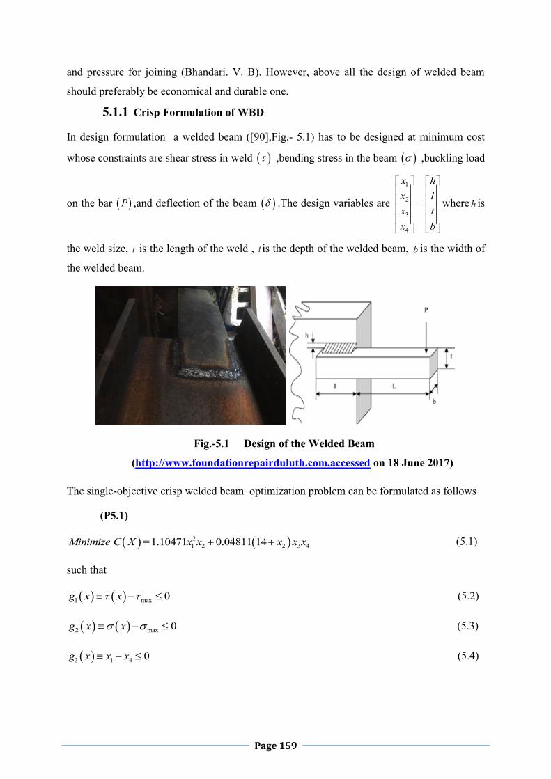
Page 159

and pressure for joining (Bhandari. V. B). However, above all the design of welded beam

should preferably be economical and durable one.

5.1.1 Crisp Formulation of WBD

In design formulation a welded beam ([90],Fig.- 5.1) has to be designed at minimum cost

whose constraints are shear stress in weld ,bending stress in the beam ,buckling load

on the bar P ,and deflection of the beam .The design variables are

1

2

3

4

x hx lx tx b

where h is

the weld size, l is the length of the weld , t is the depth of the welded beam, b is the width of

the welded beam.

Fig.-5.1 Design of the Welded Beam

(http://www.foundationrepairduluth.com,accessed on 18 June 2017)

The single-objective crisp welded beam optimization problem can be formulated as follows

(P5.1)


such that

1 max 0g x x

(5.2)

2 max 0g x x

(5.3)

3 1 4 0g x x x

(5.4)

http://www.foundationrepairduluth.com,accessed/

Page 160

24 1 2 3 4 20.10471 0.04811 14 5 0g x x x x x x

(5.5)

5 10.125 0g x x

(5.6)

6 max 0g x x

(5.7)

7 0Cg x P P x

(5.8)

1 2 3 4, , , 0,1x x x x

(5.9)

where 2 221 1 2 22

2xxR

; (5.10)

11 22

Px x

; (5.11)

2MRJ

; (5.12)

2

2xM P L

; (5.13)

221 32

4 2x xxR

; (5.14)

221 31 2 2 ;

12 22x xx x xJ

(5.15)

24 3

6 ;PLxx x

(5.16)

3

24 3

4 ;PLxEx x

(5.17)

6 63 4 3

2

4.013 / 361

2 4C

EGx x x EP xL L G

. (5.18)

Again P Force on beam ; L Beam length beyond weld; 1x Height of the welded beam;

2x Length of the welded beam; 3x Depth of the welded beam; 4x Width of the welded

beam; x Design shear stress; x Design normal stress for beam material; M

Page 161

Moment of P about the centre of gravity of the weld , J Polar moment of inertia of weld

group; G Shearing modulus of Beam Material; E Young modulus; max Design Stress

of the weld; max Design normal stress for the beam material; max Maximum deflection;

1 Primary stress on weld throat. 2 Secondary torsional stress on weld.

5.1.2 WBD Formulation in Neutrosophic Environment

Sometimes slight change of stress or deflection enhances the weight of structures and

indirectly cost of processing. In such situation when Decision Maker (DM) is in doubt to

decide the stress constraint goal, the DM can induce the idea of acceptance boundary,

hesitancy response or negative response margin of constraints goal. This fact seems to take

the constraint goal as a NS instead of FS and IFS. It may be more realistic description than

FS and IFS. When the sheer stress, normal stress and deflection constraint goals are NS in

nature the above crisp welded beam design (P5.1) can be formulated as

(P5.2)


Such that

1 maxng x x

(5.20)

2 maxng x x

(5.21)

3 1 4 0g x x x

(5.22)

24 1 2 3 4 20.10471 0.04811 14 5 0g x x x x x x

(5.23)

5 10.125 0g x x

(5.24)

6 maxng x x

(5.25)

7 0Cg x P P x

(5.26)

1 2 3 4, , , 0,1x x x x

(5.27)

Where all the parameters have their usual meaning as stated in sect.5.1.2 .Here constraint

goals are characterized by Neutrosophic Sets

max max max

max max 1 2 max 1 2 max 1 2 max 1 2, , , , , , ,n n nn x x T x x I x x F x x

(5.28)

Page 162

with max

max 1 2, ,nT x x

max

max 1 2, ,nI x x

max

max 1 2,nF x x

as the degree of truth,

indeterminacy and falsity membership function of Neutrosophic set maxn ;

max max max


(5.29)

with max

max 3 4, ,nT x x

max

max 3 4, ,nI x x

max

max 3 4,nF x x


indeterminacy and falsity membership function of Neutrosophic set maxn ; and

max max max


(5.30)

with max

max 3 4, ,nT x x

max

max 3 4, ,nI x x

max

max 3 4,nF x x


indeterminacy and falsity membership function of Neutrosophic set maxn

5.1.3 Optimization of WBD in Neutrosophic Environment

To solve the WBD (P5.2) step 1 of sect.1.29 is used and we will get optimum solutions of

two sub problem as 1X and 2X . After that according to step 2 we find upper and lower

bound of membership function of objective function as , ,T I F

C X C X C XU U U and

, ,T I FC X C X C XL L L where

1 2max , ,TC XU C X C X

(5.31)

1 2min , ,TC XL C X C X

(5.32)

Therefore

,F T F TC X C X C X C X C XU U L L where 0 T T

C X C X C XU L

(5.33)

,I T I TC X C X C X C X C XL L U L where 0 T T

C X C X C XU L

(5.34)


F T IWT WT WTU U U

F TWT WT WTL L where 0 T T

WT WT WTU L

I TWT WT WTL L where 0 T T

WT WT WTU L

Page 163

Let the linear membership functions for objective be,

1

0

TC X

TC X T T

C X C X C XT TC X C X

TC X

if C X L

U C XT C X if L C X U

U L

if C X U

(5.35)

Model-I,II-AL

1

0

TWT A

TC X C X T T

C X C X C X C XC X

TC X C X

if C X L

L C XI C X if L C X L

if WT A L

(5.36)

Model-I,II-BL

1

0

TWT A

TC X C X T T

C X C X C X WT AT TWT A WT A C X

TC X C X

if C X U

C X LI C X if L C X U

U L

if WT A L

(5.37)

0

1

TC X C X

TC X C X T T

C X C X C X C XT TC X C X C X

TC X

if C X L

C X LF C X if L C X U

U L

if C X U

(5.38)

and constraints be,

1

0

i

i

i ii

i i

i

Ti

Ti T T

i iX T T

Ti

if X L

U XT X if L X U

U L

if X U

(5.39)

Model-I,II-AL

Page 164

1

0

i

i i

i ii i

i

i i

Ti

TiX T T

i iX XX

Ti X

if X L

L XI X if L X L

if X L

(5.40)

Model-I,II-BL

1

0

i

i i

i ii i

i i i

i i

Ti

Ti X T T

i iX XT TX

Ti X

if X U

X LI X if L X U

U L

if X L

(5.41)

0

1

i i

i i

i ii i

i i i

i

Ti X

Ti X T T

i iX XT TX

Ti

if X L

X LF X if L X U

U L

if X U

(5.42)

for

01,2,..., 0 ,i i iX Xj m

Using Smarandache’s definition of intersection of neutrosophic sets and decision making

criteria NSO problem (P5.2), can be formulated as the following crisp linear programming

problem by considering linear membership as follows,

Model-I-AL

(P5.3)

Maximize (5.43)

Such that

;T T TC X C X C XC X U L U

(5.44)

;T

C X C X C XC X L

(5.45)

;T T TC X C X C X C X C XC X U L L

(5.46)

;i i i

T T Ti X X XX U L U

(5.47)

Page 165

;i i i

Ti X X XX U

(5.48)

;i i i i i

T T Ti X X X X XX U L L

(5.49)

3; (5.50)

; ; (5.51)

, , 0,1

(5.52)

Model-I-BL

(P5.4)

Maximize (5.53)

Such that


(5.54)


(5.55)


(5.56)

;i i i

T T Ti X X XX U L U

(5.57)

;i i i i i


(5.46)

;i i i i i


(5.58)

3; (5.59)

; ; (5.60)

, , 0,1

Here Model-I-AL and Model-I-BL stand for the Neutrosophic Optimization algorithm with

indeterminacy membership function of decreasing sense and increasing sense respectively.

(P5.5)

Page 166

Model-II-AL

Maximize (5.61)

Subject to


(5.62)

;T

C X C X C XC X L

(5.63)


(5.64)

;i i i

T T Ti X X XX U L U

(5.65)

;i i i

Ti X X XX L

(5.66)

;i i i i i


(5.67)

3; (5.68)

; ; (5.69)

, , 0,1

(5.70)

Model-II-BL

(P5.6)

Maximize (5.71)

Subject to


(5.72)


(5.73)


(5.74)

;i i i

T T Ti X X XX U L U

(5.75)

;i i i i i


(5.76)

Page 167

;i i i i i


(5.77)

3; (5.78)

; ; (5.79)

, , 0,1

Here Model-II-AL and Model-II-BL stand for the Neutrosophic Optimization algorithm with

indeterminacy membership function of decreasing sense and increasing sense respectively.

All these crisp nonlinear programming problem can be solved by appropriate mathematical

algorithm.

5.2 Numerical Solution of WBD by Single Objective Neutrosophic

Optimization Technique Input data of welded beam design problem (P5.1) are given in Table 5.1as follows

Table 5.1 Input Data for Neutrosophic Model (P5.2)

Applied

load P

lb

Beam

length

beyond

weld L

in

Young

Modulus

E

psi

Value of

G

psi

Maximum

allowable

shear

stress max

psi

Maximum

allowable

normal

stress max

psi

Maximum

allowable

deflection

max

in

6000 14 63 10

612 10

13600

with

allowable

tolerance

50

30000

with

allowable

tolerance

50

0.25

with

allowable

tolerance

0.05

Solution: According to step 2 of sect. 1.29, we find upper and lower bound of membership

function of objective function as , ,T I F

C X C X C XU U U and , ,T I F

C X C X C XL L L where

1.861642 , 1.858613 ,T F T IC X C X C X C XU U L L 1.858613F

C X C XL ,with

0 .003029;C X and

I TC X C X C XU L with

0 .003029C X

Page 168

Now using the bounds we calculate the membership functions for objective as follows

1 1.858613

1.8616421.858613 1.861642

.0030290 1.861642

C X

if C X

C XT C X if C X

if C X

(5.80)

For Model-I-AL

1 1.858613

1.8586131.858613 1.858613

0 1.858613

C XC X C X

C X

C X

if C X

g xI C X if C X

if C X

(5.81)

For Model-I-BL

1 1.861642

1.8586131.858613 1.861642

0.003029

0 1.858613

C XC X C X

C X

C X

if C X

g xI C X if C X

if C X

(5.82)

0 1.858613

1.8586131.858613 1.861642

.003029

1 1.861642

C X

C XC X C X

C X

if C X

C XF C X if C X

if C X

(5.83)

Similarly the membership functions for shear stress constraint are,

Page 169

1

1

11 1

1

1 13600

1360013600 13650

500 13650

g x

if g x

g xT g x if g x

if g x

(5.84)

For Model-I-AL

1

1 1

1

1

1

11 1

1

1 13600

1360013600 13600

0 13600

g xg x g x

g x

g x

if g x

g xI g x if g x

if g x

(5.85)

For Model-I-BL

1

1 1

1

1

1

11 1

1

1 13650

1360013600 13650

50

0 13600

g xg x g x

g x

g x

if g x

g xI g x if g x

if g x

(5.86)

1

1

1 1

1

1

11 1

1

0 13600

1360013600 13650

50

1 13650

g x

g xg x g x

g x

if g x

g xF g x if g x

if g x

(5.87)

1 10 , .003209g x g xwhere

and the membership functions for normal stress constraint are,

2

2

22 2

2

1 30000

3000030000 30050

500 30050

g x

if g x

g xT g x if g x

if g x

(5.88)

Page 170

For Model-I-AL

2

2 2

2

2

2

22 2

2

1 30000

3000030000 30000

0 30000

g xg x g x

g x

g x

if g x

g xI g x if g x

if g x

(5.89)

For Model-I-BL

2

2 2

2

2

2

22 2

2

1 30050

3000030000 30050

50

0 30000

g xg x g x

g x

g x

if g x

g xI g x if g x

if g x

(5.90)

2

2

2 2

2

2

22 2

2

0 30000

3000030000 30050

50

1 30050

g x

g xg x g x

g x

if g x

g xF g x if g x

if g x

(5.91)

2 20 , 50g x g xwhere

The membership functions for deflection constraint are,

6

6

66 6

6

1 0.25

0.250.25 0.3

0.050 0.3

g x

if g x

g xT g x if g x

if g x

(5.92)

For Model-I-AL

Page 171

6

6 6

6

6

6

66 6

6

1 0.25

0.250.25 0.25

0 0.25

g xg x g x

g x

g x

if g x

g xI g x if g x

if g x

(5.93)

For Model-I-BL

6

6 6

6

6

6

66 6

6

1 0.3

0.250.25 0.3

0.05

0 0.25

g xg x g x

g x

g x

if g x

g xI g x if g x

if g x

(5.94)

6

6

6 6

6

6

66 6

6

0 0.25

0.250.25 0.3

0.05

1 0.3

g x

g xg x g x

g x

if g x

g xF g x if g x

if g x

(5.95)

6 60 , .05g x g xwhere

Now, using above mentioned truth, indeterminacy and falsity linear membership function

NLP (P5.1) can be solved for Model –I-AL,BL, Model-II-AL,BL, by fuzzy, IF and NSO

technique with different values of 1 2 6

, , ,C X g x g x g x and 1 2 6

, , ,C X g x g x g x . The

optimum height, length, depth, width and cost of welding of welded beam design (P5.1) are

given in Table 5.2 and the solutions are compared with other deterministic optimization

methods.

Table 5.2 Comparison of Optimal Solution of Welded Beam Design(P5.1) based on

Fuzzy and IF and NSO Technique( Model - I and Model- II) with Different Methods

Methods Height

1x

inch

Length

2x

inch

Depth

3xinch

Width

4x

inch

Welding

cost C X

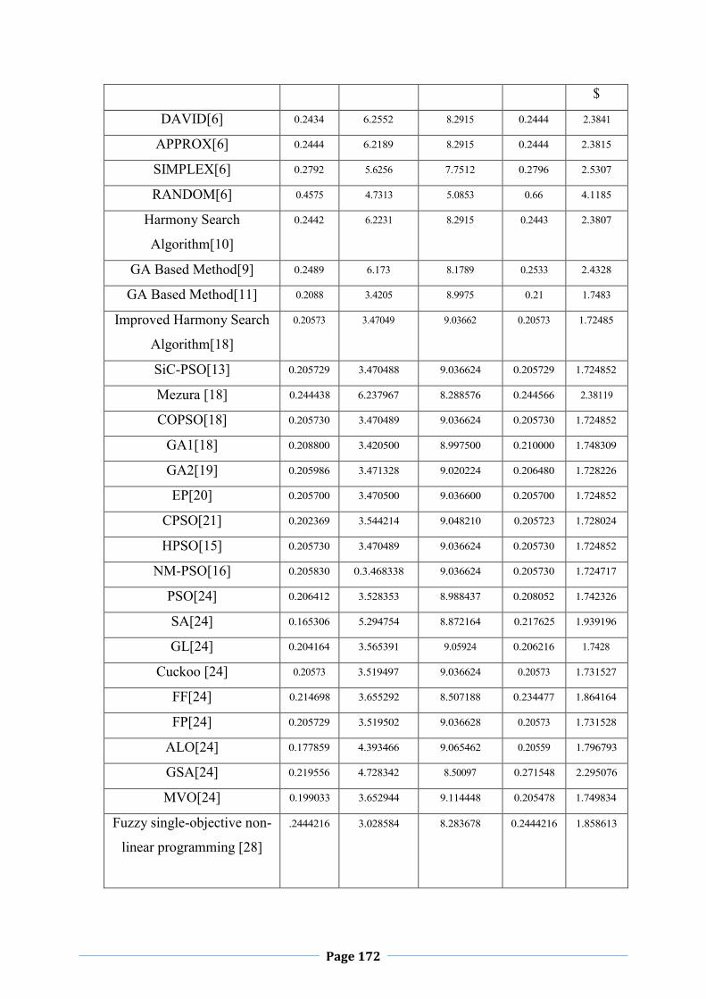
Page 172

$

DAVID[6] 0.2434

6.2552

8.2915

0.2444

2.3841

APPROX[6] 0.2444

6.2189

8.2915

0.2444

2.3815

SIMPLEX[6] 0.2792

5.6256

7.7512

0.2796

2.5307

RANDOM[6] 0.4575

4.7313

5.0853

0.66

4.1185

Harmony Search

Algorithm[10]

0.2442

6.2231

8.2915

0.2443

2.3807

GA Based Method[9] 0.2489

6.173

8.1789

0.2533

2.4328

GA Based Method[11] 0.2088

3.4205

8.9975

0.21

1.7483

Improved Harmony Search

Algorithm[18]

0.20573

3.47049

9.03662

0.20573

1.72485

SiC-PSO[13] 0.205729

3.470488

9.036624

0.205729

1.724852

Mezura [18] 0.244438

6.237967

8.288576

0.244566

2.38119

COPSO[18] 0.205730 3.470489 9.036624 0.205730 1.724852

GA1[18] 0.208800 3.420500 8.997500 0.210000 1.748309

GA2[19] 0.205986 3.471328 9.020224 0.206480 1.728226

EP[20] 0.205700 3.470500 9.036600 0.205700 1.724852

CPSO[21] 0.202369 3.544214 9.048210 0.205723 1.728024

HPSO[15] 0.205730 3.470489 9.036624 0.205730 1.724852

NM-PSO[16] 0.205830 0.3.468338 9.036624 0.205730 1.724717

PSO[24] 0.206412 3.528353 8.988437 0.208052 1.742326

SA[24] 0.165306 5.294754 8.872164 0.217625 1.939196

GL[24] 0.204164 3.565391 9.05924 0.206216 1.7428

Cuckoo [24] 0.20573 3.519497 9.036624 0.20573 1.731527

FF[24] 0.214698 3.655292 8.507188 0.234477 1.864164

FP[24] 0.205729 3.519502 9.036628 0.20573 1.731528

ALO[24] 0.177859 4.393466 9.065462 0.20559 1.796793

GSA[24] 0.219556 4.728342 8.50097 0.271548 2.295076

MVO[24] 0.199033 3.652944 9.114448 0.205478 1.749834


linear programming [28]

.2444216 3.028584 8.283678 0.2444216 1.858613

Page 173

Intuitionistic Fuzzy single-

objective non-linear

programming (FSONLP)

[28]

.0015,C X 1

25,xg

225,

xg 6

.025,xg

.2443950 3.034430 8.287578 0.2443950 1.860125

Proposed

Neutosophic

optimization(NSO)

.0015,C X

125,

xg 2

25,xg

6.025,

xg

.0024,C X

140,

xg 2

40,xg

6.04,

xg

Model-I -

AL .2443950 3.034430 8.287578 0.2443950 1.860125

Model-I-

BL NO FEASIBLE SOLUTION FOUND

Model-II-

AL .2443950 3.034430 8.287578 0.2443950 1.860125

Model-II-

BL .7308867 1.840784 2.0 .5078827 1.860419

A detailed comparison has been made among several deterministic optimization methods for

optimizing welding cost with imprecise optimization methods such as fuzzy, IF and NSO

methods in Table 5.2. It has been observed that fuzzy nonlinear optimization provides better

result in comparison with IF and NSO methods. Although it has been seen that cost of

welding is minimum other than the method studied in this paper, as far as non-deterministic

optimization methods concern ,fuzzy, IF and NSO are providing a valuable result in

imprecise environment in this chapter and literature. It has been seen that Improved Harmony

Search Algorithm[17],COPSO[17],EP[20],HPSO[15] are providing minimum most cost of

welding where all the parameters have been considered as exact in nature . However, it may

also be noted that the efficiency of the proposed method depends on the model chosen to a

greater extent because it is not always expected that NSO will provide better results over

fuzzy and IF optimization . So overall NSO is an efficient method in finding best optimal

solution in imprecise environment. It has been studied that same results have been obtained

while indeterminant membership tried to be maximize (Model- I) or minimize (Model-II) in

NSO for this particular problem.

Page 174

5.3 Conclusion

In this paper, a single objective NSO algorithm has been developed by defining truth,

indeterminacy and falsity membership function which are independent to each other. Using

this method firstly optimum height length depth, width and cost of welding have been

calculated and finally the results are compared with different deterministic methods. So

illustrated example of welded beam design has been provided to illustrate the optimization

procedure, effectiveness and advantages of the proposed NSO method. The comparison of

NSO technique with other optimization techniques has enhanced the acceptability of

proposed method .The proposed procedures has not only validated by the existing methods

but also it develops a new direction of optimization theory in imprecise environment which is

more realistic.

Page 175

CHAPTER 6Multi-Objective Welded Beam Optimization using Neutrosophic

Optimization Technique: A Comparative Study

Structural optimization, such as welded beam design optimization is an important notion in

civil engineering. Traditionally structural optimization is a well-known concept and in many

situations it is treated as single objective form, where the objective is known cost function .

The extension of this can be defined as optimization where one or more constraints are

simultaneously satisfied next to the minimization of the cost function. This does not always

hold well in real world problems where multiple and conflicting objectives frequently exist.

In this consequence a methodology known as Multi-Objective Structural Optimization

(MOSO) is introduced. Welding, a process of joining metallic parts with the application of

heat or pressure or the both, with or without added material, is an economical and efficient

method for obtaining permanent joints in the metallic parts. Most important the design of

welded beam should preferably be economical and durable one. Since decades, deterministic

optimization has been widely used in practice for optimizing welded connection design.

These include mathematical optimization algorithms (Ragsdell & Phillips [90]) such as

APPROX (Griffith & Stewart’s) successive linear approximation, DAVID (Davidon Fletcher

Powell with a penalty function), SIMPLEX (Simplex method with a penalty function), and

RANDOM (Richardson’s random method) algorithms, GA-based methods (Deb [40], Deb

[37], Coello [14], Coello [39]), particle swarm optimization (Reddy [59]), harmony search

method (Lee & Geem [67]), and Big-Bang Big-Crunch (BB-BC) (O. Hasançebi, [65])

algorithm. SOPT (O. Hasançebi, [55]), subset simulation (Li [69]), improved harmony search

algorithm (Mahadavi [72]), etc. All these deterministic optimizations aim to search the

optimum solution under given constraints without consideration of uncertainties. So, while a

deterministic optimization approach is unable to handle structural performances such as

imprecise stresses and deflection etc. due to the presence of uncertainties, to get rid of such

problem Fuzzy Set (FS)(Zadeh, [133]), Intuitionistic Fuzzy Set(IFS) (Atanassov,[1]),

Neutrosophic Set (NS)(Smarandache,[94]) play great roles. So to deal with different

impreciseness such as stresses and deflection with multiple objective ,we have been

motivated to incorporate the concept of NS in this problem, and have developed Multi-

Page 176

Objective Neutrosophic Optimization(MONSO) algorithm to optimize the optimum design.

Usually IFS, which is the generalization of FS, considers both truth membership and falsity

membership that can handle incomplete information excluding the indeterminate and

inconsistent information while NS can quantify indeterminacy explicitly by defining truth,

indeterminacy and falsity membership function independently. Therefore in 2010 Wang et.al

presented such set as Single Valued Neutrosophic set (SVNS) as it comprised of generalized

classic set, FS, interval valued FS, IFS and Para-consistent set.

As application of SVNS optimization method is rare in welded beam design, hence it is used

to minimize the cost of welding by considering shear stress, bending stress in the beam, the

buckling load on the bar, the deflection of the beam as constraints. Therefore the result has

been compared among three cited methods in each of which impreciseness has been

considered completely in different way.Moreover using above cited concept, a MONSO

algorithm has been developed to optimize three bar truss design (Sarkar et.al [107]), and to

optimize riser design problem (Das et.al [25]).However, the factors governing of former

constraints are height and length of the welded beam, forces on the beam, moment of load

about the centre of gravity of the weld group, polar moment of inertia of the weld group

respectively. The second constraint considers forces on the beam, length and size of the weld,

depth and width of the welded beam respectively. Third constraint includes height and width

of the welded beam. Fourth constraints consist of height, length, depth and width of the

welded beam. Lastly fifth constraint includes height of the welded beam. Besides, flexibility

has been given in shear stress, bending stress and deflection only, hence all these parameters

become imprecise in nature so that it can be considered as NS to form truth, indeterminacy

and falsity membership functions Ultimately, NSO technique has been applied on the basis of

the cited membership functions and outcome of such process provides the minimum cost of

welding, minimum deflection for nonlinear welded beam design. The comparison of results

shows difference between the optimum value when partially unknown information is fully

considered or not.

6.1 General Form of Multi-Objective Welded Beam Design(MOWBD)

In sizing optimization problems, the aim is to minimize multi objective function, usually the

cost of the structure, deflection under certain behavioural constraints which are displacement

or stresses. The design variables are most frequently chosen to be dimensions of the height,

length, depth and width of the structures. Due to fabrications limitations the design variables

Page 177

are not continuous but discrete for belongingness of cross-sections to a certain set. A discrete

structural optimization problem can be formulated in the following form

(P6.1)

( )Minimize C X (6.1)

Minimize X (6.2)

, 1,2,..,i isubject to X X i m (6.3)

, 1,2,...,djX R j n (6.4)

where ( ),C X X and i X as represent cost function, deflection and the behavioural

constraints respectively whereas i X denotes the maximum allowable value , ‘m’ and

‘n’ are the number of constraints and design variables respectively. A given set of discrete

value is expressed by dR and in this paper objective functions are taken as

1 1

mTtn

t nt n

C X c x

and X (6.5)

The constraints are chosen to be stress of structures as follows

i iA With allowable tolerance 0i for 1,2,....,i m (6.6)

Where tc is the cost coefficient of tth side and nx is the thn design variable respectively, m is

the number of structural element, i and 0i are the thi stress , allowable stress respectively.

6.2 Solution of Multi-Objective Welded Beam Design (MOWBD)

Problem by Neutrosophic Optimization(NSO) Technique

To solve the MOSOP (P6.1), step 1 of 1.33 is used .After that according to step to pay off

matrix is formulated.

* 1 11

2 2 * 2

C X X

C X XXX C X X

According to step-2 the bound of weight objective , ;T T

C X C XU L ,I IC X C XU L and

,F FC X C XU L

for truth, indeterminacy and falsity membership function respectively. Then

Page 178

;T TC X C XL C X U (6.7)

;I IC X C XL C X U (6.8)

F FC X C XL C X U (6.9)

Similarly the bound of deflection objective are , ; , ,T T I I F FX X X X X XU L U L and U L

are

respectively for truth, indeterminacy and falsity membership function. Then

;T T

X XL X U

(6.10)

;I I

X XL X U

(6.11)

F F

X XL X U

. (6.12)

Where ,for Model-I,II-AL,AN

,F TC X C XU U

(6.13)

;F TC X C X C XL L (6.14)

,I TC X C XL L (6.15)

I TC X C X C XU L (6.16)

0 , T TC X C X C X C XU L


F T IC X C X C XU U U

F TC X C X C XL L where 0 T T

C X C X C XU L

I TC X C X C XL L where 0 T T

C X C X C XU L

And for Model-I,II-AL,AN

,F T

X XU U

(6.17)

;F T

X X XL L

(6.18)

,I T

X XL L

(6.19)

I T

X X XU L

(6.20)

such that

Page 179

0 , T TX X X XU L

.


F T I

X X XU U U

F T

X X XL L

where 0 T TX X XU L

I T

X X XL L

where 0 T TX X XU L

Therefore the truth, indeterminacy and falsity membership functions for objectives are

1

1 exp

0

TC X

TC X T T

C X C X C XT TC X C X

TC X

if C X L

U C XT C X if L C X U

U L

if C X U

(6.21)

For Model-I,II-AN

1

exp

0

TC X

TC X C X T T

C X C X C X C XC X

TC X C X

if C X L

L C XI C X if L C X L

if C X L

(6.22)

For Model-I,II-BN

1

exp

0

TC X

TC X C X T T

C X C X C X C XT TC X C X C X

TC X C X

if C X U

C X LI C X if L C X U

U L

if C X L

(6.23)

Page 180

0

1 1 tanh2 2 2

1

TC X C X

T TC X C X C X T T

C X C X C X C X C X

TC X

if C X L

U LF C X C X if L C X U

if C X U

(6.24)

0 , T TC X C X C X C Xwhere U L

and

1

1 exp

0

TX

TX T T

X X XT TX X

TX

if X L

U XT X if L X U

U L

if X U

(6.25)

Model-I,II-AN

1

exp

0

T

TX X T T

X X X XX

TX X

if X L

L XI X if L X L

if X L

(6.26)

Model-I,II-AN

Model-I,II-BN

1

exp

0

T

TX X T T

X X XT TX

TX X

if X U

X LI X if L X U

U L

if X L

(6.27)

0

1 1 tanh2 2 2

1

TX X

T TX X X T T

X X X X X

TX

if X L

U LF X X if L X U

if X U

(6.28)

Page 181


0 , T TX X X Xwhere U L

According to Smarandache’s definition of intersection of neutrosophic sets and decision

making criteria NSO algorithm for MOSOP (P6.1) can be formulated as

Model-I-AN,BN

(P6.2)

Maximize (6.29)

Subject to

;C XT C X (6.30)

;XT X

(6.31)

;C XI C X (6.32)

;XI X

(6.33)

;C XF C X (6.34)

;XF X

(6.35)

;i iX X (6.36)

3; (6.37)

; ; (6.38)

, , 0,1 , (6.39)

min maxX X X (6.40)

But in realworld decision making problem a decision maker needs to minimize indeterminacy

membership function.So the optimization algorithm problem can be formulated as

Model-II-AN,BN

(P6.3)

Maximize (6.41)

Subject to

;C XT C X (6.42)

;XT X

(6.43)

Page 182

;C XI C X (6.44)

;XI X

(6.45)

;C XF C X (6.46)

;XF X

(6.47)

;i iX X (6.48)

3; (6.49)

; ; (6.50)

, , 0,1 , (6.51)

min maxX X X

Here Model-IAN andModel-IBN stands for neutrosophic algorithm with indeterminacy

membership function as decreasing sense and increasing sense respectively, which is

reduced to equivalent non linear programming problem as

Model-I-AN

(P6.4)

Maximize

Such that

;T TC X C X T

C X

U LC X U

(6.52)

;2

T TC X C X C X

C X

U LC X

(6.53)

;T

C X C X C XC X L (6.54)

;T T

X X TX

U LX U

(6.55)

;T

X X XX L

(6.56)

;2

T TX X X

X

U LX

(6.57)

;i iX X (6.58)

3; (6.59)

; ; (6.60)

Page 183

, , 0,1 (6.61)

min maxX X X (6.62)

where ln 1 ;

(6.63)

4; (6.64)

6 ;C X F F

C X C XU L

(6.65)

6 ;X F F

X XU L

(6.66)

ln ; (6.67)

1tanh 2 1 . (6.68)

Model-I-BN

(P6.5)

Maximize

Such that

;T TC X C X T

C X

U LC X U

(6.69)

;2

T TC X C X C X

C X

U LC X

(6.70)

;T T TC X C X C X C X C XC X U L L (6.71)

;T T

X X TX

U LX U

(6.72)

;T T T

X X X X XX U L L

(6.73)

;2

T TX X X

X

U LX

(6.74)

;i iX X (6.75)

3; (6.76)

; ; (6.77)

, , 0,1 (6.78)

Page 184

min maxX X X (6.79)

where ln 1 ;

(6.80)

4; (6.81)

6 ;C X F F

C X C XU L

(6.82)

6 ;X F F

X XU L

(6.83)

ln ; (6.84)

1tanh 2 1 . (6.85)

Model-II-AN

(P6.6)

Maximize (6.86)

Such that

;T TC X C X T

C X

U LC X U

(6.87)

;2

T TC X C X C X

C X

U LC X

(6.88)

;T

C X C X C XC X L (6.89)

;T T

X X TX

U LX U

(6.90)

;T

X X XX L

(6.91)

;2

T TX X X

X

U LX

(6.92)

;i iX X (6.93)

3; (6.94)

; ; (6.95)

, , 0,1 (6.96)

min maxX X X (6.97)

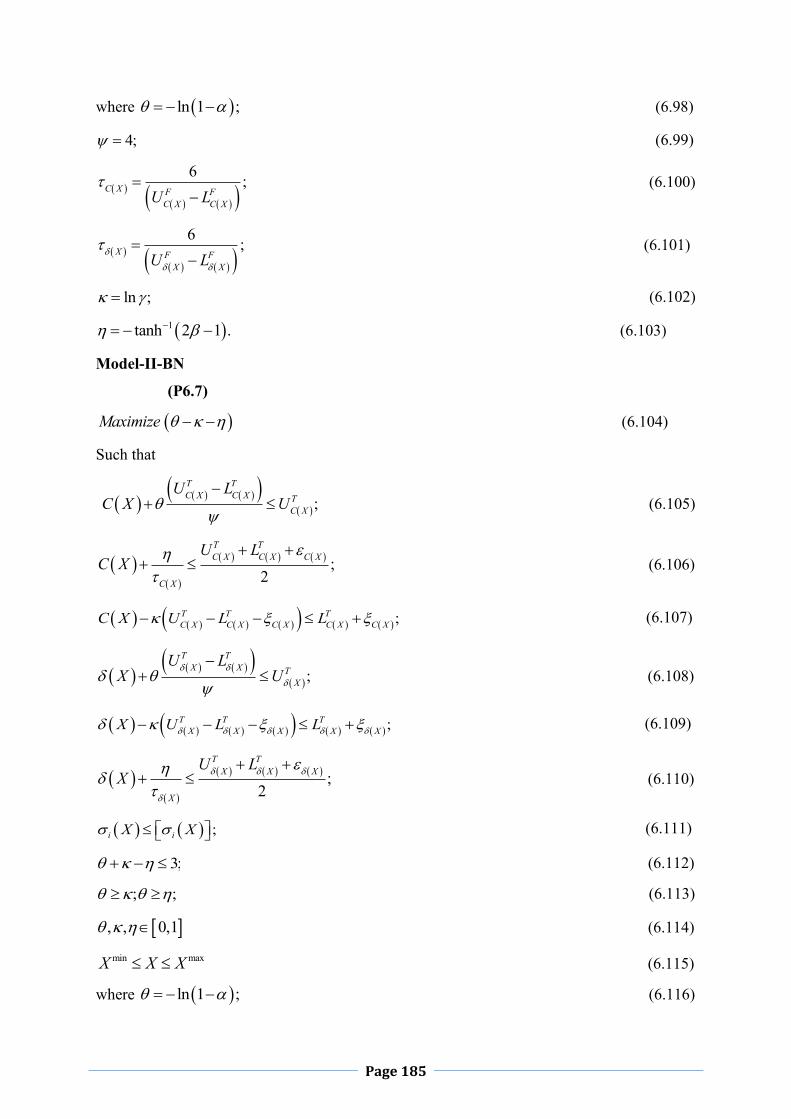
Page 185

where ln 1 ;

(6.98)

4; (6.99)

6 ;C X F F

C X C XU L

(6.100)

6 ;X F F

X XU L

(6.101)

ln ; (6.102)

1tanh 2 1 . (6.103)

Model-II-BN

(P6.7)

Maximize (6.104)

Such that

;T TC X C X T

C X

U LC X U

(6.105)

;2

T TC X C X C X

C X

U LC X

(6.106)

;T T TC X C X C X C X C XC X U L L (6.107)

;T T

X X TX

U LX U

(6.108)

;T T T

X X X X XX U L L

(6.109)

;2

T TX X X

X

U LX

(6.110)

;i iX X (6.111)

3; (6.112)

; ; (6.113)

, , 0,1 (6.114)

min maxX X X (6.115)

where ln 1 ;

(6.116)

Page 186

4; (6.117)

6 ;C X F F

C X C XU L

(6.118)

6 ;X F F

X XU L

(6.119)

ln ; (6.120)

1tanh 2 1 .

(6.121)

Solving the above crisp model (P6.4),(P6.5),(P6.6),(P6.7) by an appropriate mathematical

programming algorithm we get optimal solution and hence objective functions i.e minimum

cost and deflection of the beam will attain optimal solution.

6.3 Numerical Solution of Welded Beam Design using Multi-Objective

Neutrosophic Optimization Technique

A welded beam (Ragsdell and Philips 1976,Fig.-6.1) has to be designed at minimum cost

whose constraints are shear stress in weld ,bending stress in the beam ,buckling

load on the bar P ,and deflection of the beam .The design variables are

1

2

3

4

x hx lx tx b

where h is the weld size, l is the length of the weld , t is the depth of the welded beam, b is

the width of the welded beam.

Fig.-6.1 Design of the Welded Beam(Cracked Beam Onsite Welding,

http://www.allmetalweldingservices.co.uk,accessed on 19 June 2017 )

http://www.allmetalweldingservices.co.uk,accessed/

Page 187


(P6.8)

21 2 2 3 41.10471 0.04811 14Minimize g x x x x x x (6.122)

3

24 3

4 ;PLMinimize xEx x

(6.123)

Such that

1 max 0;g x x (6.124)

2 max 0;g x x (6.125)

3 1 4 0;g x x x (6.126)

24 1 2 3 4 20.10471 0.04811 14 5 0;g x x x x x x (6.127)

5 10.125 0;g x x (6.128)

6 max 0;g x x (6.129)

7 0;Cg x P P x (6.130)

1 4 2 30.1 , , , 2.0x x x x

where 2 221 1 2 22

2xxR

; (6.131)

11 22

Px x

; (6.132)

2MRJ

; (6.133)

2

2xM P L

; (6.134)

221 32

4 2x xxR

; (6.135)

221 31 2 2 ;

12 22x xx x xJ

(6.136)

24 3

6 ;PLxx x

(6.137)

3

24 3

4 ;PLxEx x

(6.138)

Page 188

6 63 4 3

2

4.013 / 361 ;

2 4C

EGx x x EP xL L G

(6.139)

P Force on beam ; L Beam length beyond weld; 1x Height of the welded beam; 2x

Length of the welded beam; 3x Depth of the welded beam; 4x Width of the welded





1 Primary stress on weld throat. 2 Secondary torsional stress on weld. Input data are

given in Table 6.1.


Applied

load P

lb

Beam

length

beyond

weld

L

in

Young

Modulus

E

psi

Value of

G

psi

Maximum

allowable

shear

stress max

psi

Maximum

allowable

normal

stress max

psi

6000 14 63 10

612 10

13600 30000

Solution: According to step 2 of 1.33, pay-off matrix is formulated as follows

1

2

7.700387 0.245136311.91672 0.1372000

C X X

XX

.

Here

11.91672,F TC X C XU U (6.140)

1 17.700387 ;F TC X C XL L (6.141)

7.700387,I TC X C XL L (6.142)

Page 189

1 17.700387I TC X C XU L (6.143)

such that 1 10 , 11.91672 7.700387 ; (6.144)

0.2451363,F TX XU U

(6.145)

2 2.1372000 ;F TX XL L

(6.146)

0.1372000,I TX XL L

(6.147)

2 20.1372000I TX XU L

(6.148)

such that 2 20 , 0.2451363 0.1372000

Here truth, indeterminacy, and falsity membership function for objective functions

,C X X are defined as follows

1 7.700387

11.916721 exp 4 7.700387 11.91672

4.216333

0 11.91672

C X

if C X

C XT C X if C X

if C X

(6.149)

For Model-I,II-AN

11

1

1

1 7.700387

7.700387exp 7.700387 7.700387

0 7.700387

C X

if C X

C XI C X if C X

if C X

(6.150)

For Model-I,II-BN

11

1

1

1 11.91672

7.700387exp 7.700387 11.91672

4.2163330 7.700387

C X

if C X

C XI C X if C X

if C X

(6.151)

1

1

0 7.700387

19.6171071 1 6tanh 7.700387 11.916722 2 2 4.216333

1 11.91672

C X

if C X

F C X C X if C X

if C X

(6.152)

1 10 , 4.216333

and

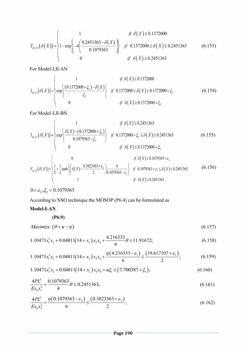
Page 190

1 0.1372000

0.24513631 exp 4 0.1372000 0.2451363

0.1079363

0 0.2451363

X

if X

XT X if X

if X

(6.153)

For Model-I,II-AN

22

2

2

1 0.1372000

0.1372000exp 0.1372000 0.1372000

0 0.1372000

X

if X

XI X if X

if X

(6.154)

For Model-I,II-BN

22

2

2

1 0.2451363

0.1372000exp 0.1372000 0.2451363

0.10793630 0.1372000

X

if X

XI X if X

if X

(6.155)

2

22

2

0 0.1079363

0.38233631 1 6tanh 0.1079363 0.24513632 2 2 0.1079363

1 0.2451363

X

if X

F X X if X

if X

(6.156)

2 20 , 0.1079363

According to NSO technique the MOSOP (P6.4) can be formulated as

Model-I-AN

(P6.9)

Maximize (6.157)

21 2 2 3 4

4.2163331.10471 0.04811 14 11.91672;4

x x x x x (6.158)

1 12

1 2 2 3 4

4.216333 19.6171071.10471 0.04811 14 ;

6 2x x x x x

(6.159)

21 2 2 3 4 1 11.10471 0.04811 14 7.700387 ;x x x x x (6.160)

3

24 3

4 0.1079363 0.2451363;4

PLEx x

(6.161)

32 2

24 3

0.1079363 0.38233634 ;6 2

PLEx x

(6.162)

Page 191

3

2 224 3

4 0.1372000 ;PLEx x

(6.163)

1 max 0;g x x (6.164)

2 max 0;g x x (6.165)

3 1 4 0;g x x x (6.166)

5 10.125 0;g x x (6.167)

6 max 0;g x x (6.168)

7 0;Cg x P P x (6.169)

1 4 2 30.1 , , , 2.0x x x x (6.170)

3; ; (6.171)

ln 1 ;

(6.172)

4; (6.173)

6 ;C X F F

C X C XU L

(6.174)

6 ;X F F

X XU L

(6.175)

ln ; (6.176)

1tanh 2 1 . (6.177)

2 221 1 2 22

2xxR

; (6.178)

11 22

Px x

; (6.179)

2MRJ

; (6.180)

2

2xM P L

; (6.181)

221 32

4 2x xxR

; (6.182)

221 31 2 2 ;

12 22x xx x xJ

(6.183)

Page 192

24 3

6 ;PLxx x

(6.184)

3

24 3

4 ;PLxEx x

(6.185)

6 63 4 3

2

4.013 / 361 ;

2 4C

EGx x x EP xL L G

(6186)

Model-I-BN

(P6.10)

Maximize

(6.187)

21 2 2 3 4

4.2163331.10471 0.04811 14 11.91672;4

x x x x x

(6.188)

1 12

1 2 2 3 4

4.216333 19.6171071.10471 0.04811 14 ;

6 2x x x x x

(6.189)

21 2 2 3 4 1 11.10471 0.04811 14 4.216333 7.700387 ;x x x x x

(6.190)

3

24 3

4 0.1079363 0.2451363;4

PLEx x

(6.191)

32 2

24 3

0.1079363 0.38233634 ;6 2

PLEx x

(6.192)

3

2 224 3

4 0.1079363 0.1372000 ;PLEx x

(6.193)

1 max 0;g x x

(6.194)

2 max 0;g x x

(6.195)

3 1 4 0;g x x x

(6.196)

5 10.125 0;g x x

(6.197)

6 max 0;g x x

(6.198)

7 0;Cg x P P x

(6.199)

1 4 2 30.1 , , , 2.0x x x x

(6.200)

3; ; (6.201)

ln 1 ;

(6.202)

4; (6.203)

Page 193

6 ;C X F F

C X C XU L

(6.204)

6 ;X F F

X XU L

(6.205)

ln ; (6.206)

1tanh 2 1 . (6.207)

2 221 1 2 22

2xxR

; (6.208)

11 22

Px x

; (6.209)

2MRJ

; (6.210)

2

2xM P L

; (6.211)

221 32

4 2x xxR

; (6.212)

221 31 2 2 ;

12 22x xx x xJ

(6.213)

24 3

6 ;PLxx x

(6.214)

3

24 3

4 ;PLxEx x

(6.215)

6 63 4 3

2

4.013 / 361 ;

2 4C

EGx x x EP xL L G

(6.216)

Model-II-AN

(P6.11)

Maximize (6.217)

21 2 2 3 4

4.2163331.10471 0.04811 14 11.91672;4

x x x x x (6.218)

1 12

1 2 2 3 4

4.216333 19.6171071.10471 0.04811 14 ;

6 2x x x x x

(6.219)

21 2 2 3 4 1 11.10471 0.04811 14 7.700387 ;x x x x x (6.220)

Page 194

3

24 3

4 0.1079363 0.2451363;4

PLEx x

(6.221)

32 2

24 3

0.1079363 0.38233634 ;6 2

PLEx x

(6.222)

3

2 224 3

4 0.1372000 ;PLEx x

(6.223)

1 max 0;g x x (6.224)

2 max 0;g x x (6.225)

3 1 4 0;g x x x (6.226)

5 10.125 0;g x x (6.227)

6 max 0;g x x (6.228)

7 0;Cg x P P x (6.229)

1 4 2 30.1 , , , 2.0x x x x (6.230)

3; ; (6.231)

ln 1 ;

(6.232)

4; (6.233)

6 ;C X F F

C X C XU L

(6.234)

6 ;X F F

X XU L

(6.235)

ln ; (6.236)

1tanh 2 1 . (6.237)

2 221 1 2 22

2xxR

; (6.238)

11 22

Px x

; (6.239)

2MRJ

; (6.240)

2

2xM P L

; (6.241)

Page 195

221 32

4 2x xxR

; (6.242)

221 31 2 2 ;

12 22x xx x xJ

(6.243)

24 3

6 ;PLxx x

(6.244)

3

24 3

4 ;PLxEx x

(6.245)

6 63 4 3

2

4.013 / 361 ;

2 4C

EGx x x EP xL L G

(6.246)

Model-II-BN

(P6.12)

Maximize (6.247)

21 2 2 3 4

4.2163331.10471 0.04811 14 11.91672;4

x x x x x (6.248)

1 12

1 2 2 3 4

4.216333 19.6171071.10471 0.04811 14 ;

6 2x x x x x

(6.249)

21 2 2 3 4 1 11.10471 0.04811 14 4.216333 7.700387 ;x x x x x (6.250)

3

24 3

4 0.1079363 0.2451363;4

PLEx x

(6.251)

32 2

24 3

0.1079363 0.38233634 ;6 2

PLEx x

(6.252)

3

2 224 3

4 0.1079363 0.1372000 ;PLEx x

(6.253)

1 max 0;g x x (6.254)

2 max 0;g x x (6.255)

3 1 4 0;g x x x (6.256)

5 10.125 0;g x x (6.257)

6 max 0;g x x (6.258)

7 0;Cg x P P x (6.259)

Page 196

1 4 2 30.1 , , , 2.0x x x x

(6.260)

3; ; (6.261)

ln 1 ;

(6.262)

4; (6.263)

6 ;C X F F

C X C XU L

(6.264)

6 ;X F F

X XU L

(6.265)

ln ; (6.266)

1tanh 2 1 . (6.267)

2 221 1 2 22

2xxR

; (6.268)

11 22

Px x

; (6.269)

2MRJ

; (6.270)

2

2xM P L

; (6.271)

221 32

4 2x xxR

; (6.272)

221 31 2 2 ;

12 22x xx x xJ

(6.273)

24 3

6 ;PLxx x

(6.274)

3

24 3

4 ;PLxEx x

(6.275)

6 63 4 3

2

4.013 / 361 ;

2 4C

EGx x x EP xL L G

(6.276)

Now , using above mentioned truth, indeterminacy and falsity membership function NLP (P6.9) ,(P6.10),(P6.11),(P6.12)can be solved by NSO technique for different values of

,g x x and ,g x x

. The optimum solution of MOSOP(P6.8) is given in Table 6.2 .

Page 197

Table 6.2 Comparison of Optimal Solution of MOSOP (P6.7) based on Different Methods

Methods

1xinch

2xinch

3xinch

4xinch

C X X

Fuzzy single-objective non-linear programming (FSONLP)

1.298580 0.9727729 1.692776 1.298580 3.395620 0.2456363

Intuitionistic Fuzzy single-objective non-linear programming (IFSONLP)

0.42,g x 0.01,x

1.298580 0.9727730 1.692776 1.298580 3.395620 0.2352203

Neutosophic optimization(NSO)

0.42,g x 0.42,g x

0.01,x 0.01,x

Model-I-AN

1.957009 1.240976 2 1.957009 8.120387 0.1402140


0.42,g x 0.42,g x

0.01,x 0.01,x

Model-I-BN

NO FEASIBLE

SOLUTION

FOUND


0.42,g x 0.42,g x

0.01,x 0.01,x

Model-II-AN

2 1.588365 2 2 10.01855 0.1961680


0.42,g x 0.42,g x

0.01,x 0.01,x

Model-II-BN

1.940309 1.246993 2 2 8.120387 0.1472

A detailed comparison has been made among the minimum length, depth, height and width of

the weld, welding cost and deflection while they have been compared among fuzzy,

intuitionistic, NSO technique in perspective of welded beam design in Table 6.2. It has been

observed that IF nonlinear optimization provides better result in comparison with other

mentioned method in this study. However, it may also be noted that the efficiency of the

proposed method depends on the model chosen to a greater extent. In the present study it has

also been investigated that that cost of welding is maximum and deflection is minimum in

NSO technique compared to the other method investigated.

6.4 Conclusion

In this chapter, a multi objective NSO algorithm has been developed by defining truth,

indeterminacy and falsity membership function which are independent to each other. It has

been shown that the developed algorithm can be applied to optimize a multi objective

nonlinear structural design. Simulation example, i.e. welded beam design has been provided

to illustrate the optimization procedure, effectiveness and advantages of the proposed NSO method. The extension of the proposed optimization can be NSO by using ranking method of

neutrosophic numbers , considered for height, length, depth and width of weld and applied

load as further topics of interest.

Page 198

CHAPTER 7Multi-Objective Welded Beam Optimization using Neutrosophic

Goal Programming Technique

With ever increasing demand for both high production rates and high precision, fully

mechanized or automated welding processes have taken a prominent place in the welding

field. Welding is the process of joining together two pieces of metal so that bonding takes

place at their original boundary surfaces. When two parts are to be joined with or without

added metal for formation of metallic bond, they are melted together by heat or pressure or

by both. The welding process is divided into two major categories: Plastic Welding or

Pressure Welding and Fusion Welding or Non-Pressure Welding. However, above all the

design of welded beam should preferably be economical and durable one. Since decades,

deterministic optimization has been widely used in practice for optimizing welded connection

design. These include mathematical optimization algorithms (Ragsdell & Phillips [90]) such

as APPROX (Griffith & Stewart’s) successive linear approximation, DAVID (Davidon

Fletcher Powell with a penalty function), SIMPLEX (Simplex method with a penalty

function), and RANDOM (Richardson’s random method) algorithms, GA-based methods

(Deb [40], Deb [37], Coello [14], Coello [39]), particle swarm optimization (Reddy [59]),

harmony search method (Lee & Geem [67]), and Big-Bang Big-Crunch (BB-BC) (O.

Hasançebi, [65]) algorithm. SOPT (O. Hasançebi, [55]), subset simulation (Li [73]),

improved harmony search algorithm (Mahadavi [72]), were other methods used to solve this

problem. Recently a robust and reliable H∞ static output feedback (SOF) control for

nonlinear systems (Yanling Wei 2016[128]) and for continuous-time nonlinear stochastic

systems (Yanling Wei [29]) with actuator fault in a descriptor system framework have been

studied. All these deterministic optimizations aim to search the optimum solution under given

constraints without consideration of uncertainties. So, while a deterministic optimization

approach is unable to handle structural performances such as imprecise stresses and

deflection etc. due to the presence of uncertainties, to get rid of such problem Fuzzy Set

(FS)(Zadeh, [133]), Intuitionistic Fuzzy Set (IFS)(Atanassov,[1]), Neutrosophic Set (NS)

(Smarandache,[94]) play great roles. Traditionally structural design optimization is a well-

known concept and in many situations it is treated as single objective form, where the

Page 199

objective is known the weight or cost function. The extension of this is the optimization

where one or more constraints are simultaneously satisfied next to the minimization of the

weight or cost function. This does not always hold good in real world problems where

multiple and conflicting objectives frequently exist. In this consequence a methodology

known as multi-objective optimization is introduced. So to deal with different impreciseness

such as stresses and deflection with multiple objective , we have been motivated to

incorporate the concept of NS in this problem, and have developed Multi-Objective

Neutrosophic Optimization(MONSO) algorithm to optimize the optimum design. Usually

IFS, which is the generalization of FS, considers both truth membership and falsity

membership that can handle incomplete information excluding the indeterminate and

inconsistent information while NS can quantify indeterminacy explicitly by defining truth,

indeterminacy and falsity membership function independently. Therefore, in 2010 Wang et.al

presented such set as Single Valued Neutrosophic Set (SVNS) as it comprised of generalized

classic set, FS, interval valued FS, IFS and Para-consistent set. As application of SVNS

optimization method, it is rare in welded beam design; hence it is used to minimize the cost

of welding by considering shear stress, bending stress in the beam, the buckling load on the

bar, the deflection of the beam as constraints. Moreover using above cited concept, a

MONSO algorithm has been developed to optimize three bar truss design (Sarkar [107]), and

to optimize riser design problem (Das [25]). In early 1961 Charnes and Cooper[24] first

introduced Goal programming problem for a linear model. Usually conflicting goal are

presented in a multi-objective goal programming problem. Actually objective goals of

existing structural model are considered to be deterministic and a fixed quantity. In a

situation ,the decision maker can be doubtful with regard to accomplishment of the goal .The

DM may include the idea of truth, indeterminacy and falsity bound on objectives goal.The

goal may have a target value with degree of truth, indeterminacy as well as degree of falsity.

Precisely, we can say a human being can express degree of truth membership of a given

element in a FS, truth and falsity membership in a IFS, but very often does not express the

corresponding degree of indeterminacy membership as complement to truth and falsity

membership which are independent. This fact seems to take the objective goal as a NS. Dey

et al[41]. used intuitionistic goal programming on nonlinear structural model.

This is the first time Neutrosophic Goal Programming (NGP) technique is in application to

multi-objective welded beam design. The present study investigates computational algorithm

for solving multi-objective welded beam problem by single valued generalized NGP

technique. The results are compared numerically for different aggregation method of NGP

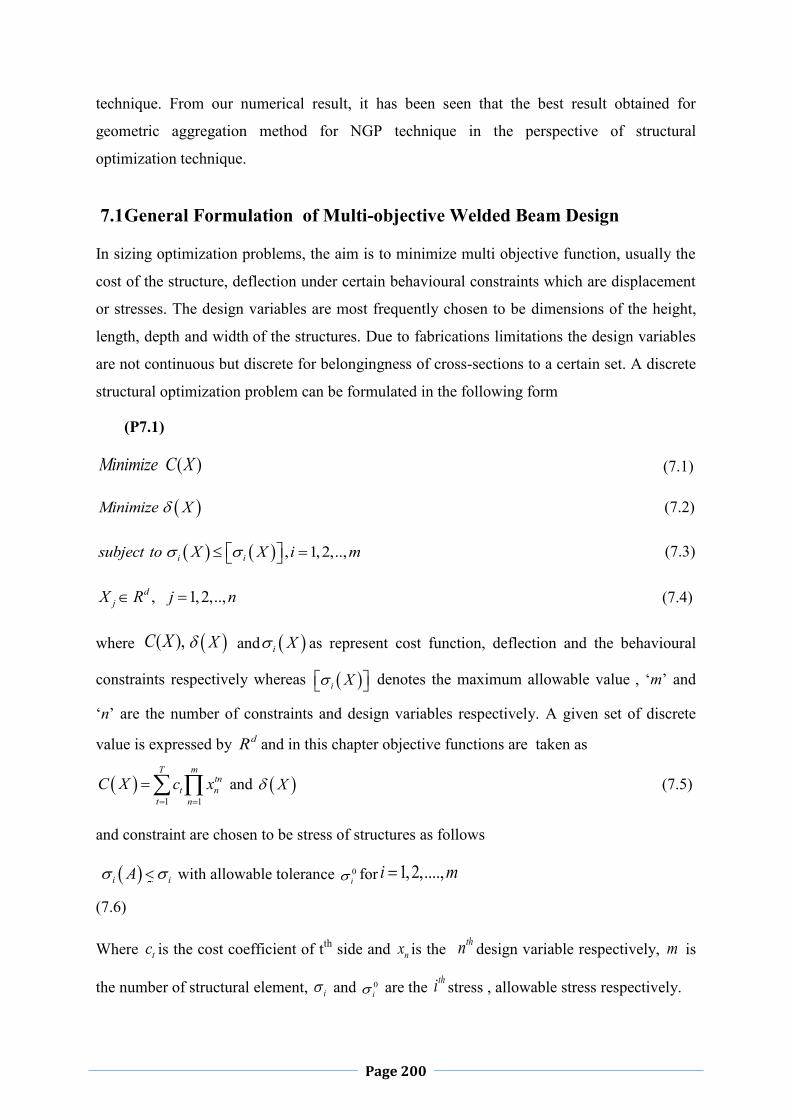
Page 200

technique. From our numerical result, it has been seen that the best result obtained for

geometric aggregation method for NGP technique in the perspective of structural

optimization technique.

7.1 General Formulation of Multi-objective Welded Beam Design

In sizing optimization problems, the aim is to minimize multi objective function, usually the

cost of the structure, deflection under certain behavioural constraints which are displacement

or stresses. The design variables are most frequently chosen to be dimensions of the height,

length, depth and width of the structures. Due to fabrications limitations the design variables

are not continuous but discrete for belongingness of cross-sections to a certain set. A discrete


(P7.1)


Minimize X

(7.2)

, 1,2,..,i isubject to X X i m (7.3)

, 1,2,..,djX R j n

(7.4)

where ( ),C X X and i X as represent cost function, deflection and the behavioural

constraints respectively whereas i X denotes the maximum allowable value , ‘m’ and

‘n’ are the number of constraints and design variables respectively. A given set of discrete

value is expressed by dR and in this chapter objective functions are taken as

1 1

mTtn

t nt n

C X c x

and X (7.5)


i iA with allowable tolerance 0i for 1,2,....,i m

(7.6)


the number of structural element, i and 0i are the thi stress , allowable stress respectively.

Page 201

7.2 Generalized Neutrosophic Goal Optimization Technique to Solve

Multi-objective Welded Beam Optimization Problem (MOWBP) The multi-objective neutrosophic structural model can be expressed as

(P7.2)

Minimize C X with target value 0C ,truth tolerance Ca ,indeterminacy tolerance Cd and

rejection tolerance Cc (7.7)

Minimize X with target value 0 ,truth tolerance 0

a ,indeterminacy tolerance

0d

and

rejection tolerance 0

c (7.8)

subject to X

(7.9)

min maxi i ix x x

(7.10)

where 1 2, ,...., TnX x x x are the design variables, n is the group number of design variables

for the welded beam design.

To solve this problem we first calculate truth ,indeterminacy and falsity membership function

of objective as follows

1

1 0

01 0 0

00

CwC C

C

C

w if C X C

C a C XT C X w if C C X C a

aif C X C a

(7.11)

2

0

02 0 0

02 0 0

0

0

0

CCw

C XC

C CC C

C

if C X C

C X Cw if C C X C a

dI C X

C a C Xw if C d C X C a

a dif C X C a

(7.12)

where 1

1 2C

C C

wd w wa c

(7.13)

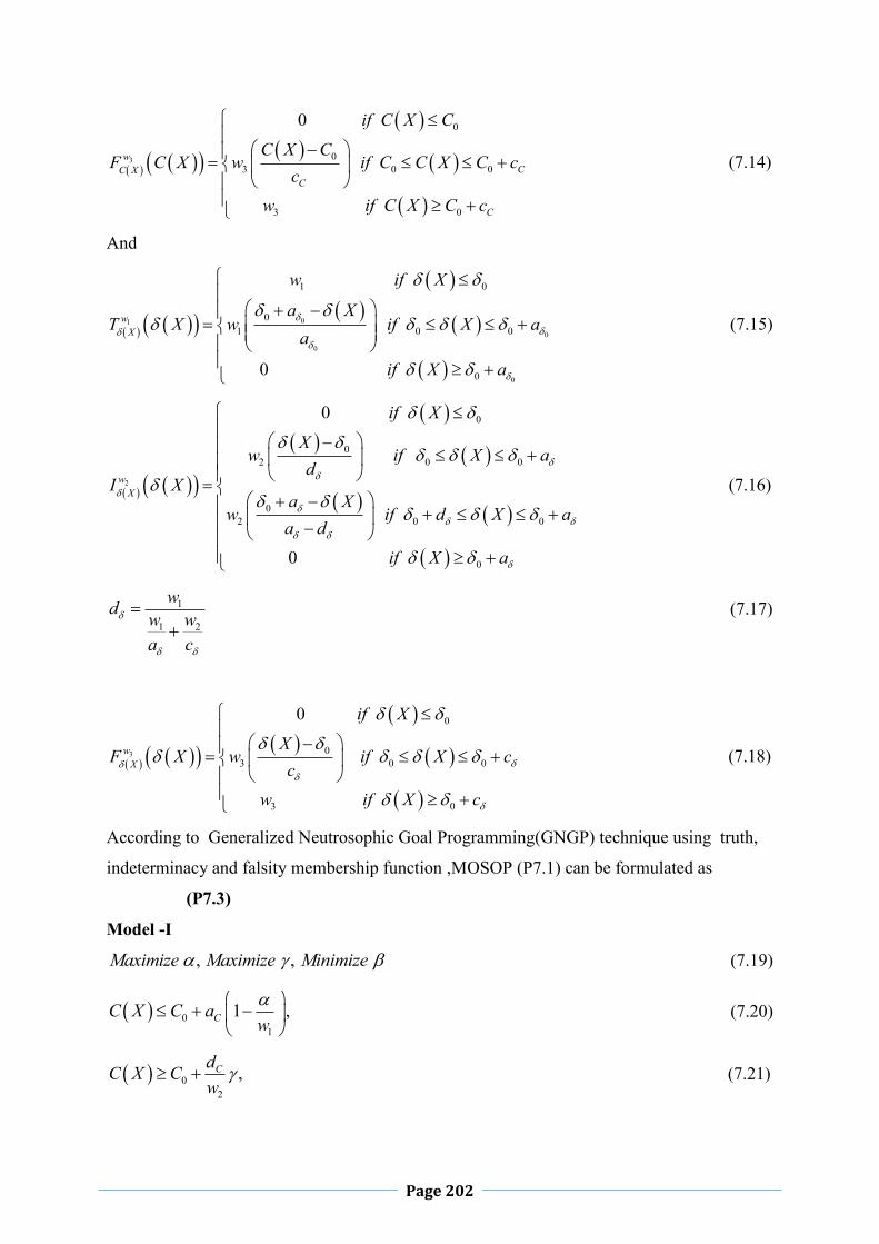
Page 202

3

0

03 0 0

3 0

0

wCC X

C

C

if C X C

C X CF C X w if C C X C c

cw if C X C c

(7.14)

And

01

0

0

0

1 0

01 0 0

00

wX

w if X

a XT X w if X a

a

if X a

(7.15)

2

0

02 0 0

02 0 0

0

0

0

wX

if X

Xw if X a

dI X

a Xw if d X a

a dif X a

(7.16)

1

1 2

wd w wa c

(7.17)

3

0

03 0 0

3 0

0

wX

if X

XF X w if X c

cw if X c

(7.18)

According to Generalized Neutrosophic Goal Programming(GNGP) technique using truth,

indeterminacy and falsity membership function ,MOSOP (P7.1) can be formulated as

(P7.3)

Model -I

,Maximize ,Maximize Minimize (7.19)

01

1 ,CC X C aw

(7.20)

02

,CdC X Cw

(7.21)

Page 203

02

,C C CC X C a a dw

(7.22)

03

,CcC X Cw

(7.23)

0 ,C X C

(7.24)

01

1 ,X aw

(7.25)

02

,dXw

(7.26)

02

,X a a dw

(7.27)

03

,cXw

(7.28)

0 ,X

(7.29)

1 2 30 ;w w w

(7.30)

1 2 30, , 0, , 0, ;w w w

(7.31)

1 2 30,1 , 0,1 , 0,1 ;w w w

(7.32)

1 2 30 3;w w w

(7.33)

, 1,2,...,i X i m

(7.34)

0, 1,2,....,jx j n

(7.35)


based on arithmetic aggregation operator (P7.1)can be formulated as

(P7.4)

Model -II

1 13

Minimize

(7.36)

Subjected to same constraint as Model I


based on geometric aggregation operator(P7.1) can be formulated as

(P7.5)

Model -III

Page 204

3 1 1Minimize

(7.37)

Subjected to same constraint as Model I

Now these non-linear programming Model-I,II,III can be easily solved through an

appropriate mathematical programming to give solution of MONLPP (P7.1) by GNGP

approach.

7.3 Numerical Solution of welded Beam Design by GNGP, based on

Different Operator A welded beam (Ragsdell and Philips 1976,Fig.- 7.1) has to be designed at minimum cost

whose constraints are shear stress in weld ,bending stress in the beam ,buckling load

on the bar P ,and deflection of the beam .The design variables are

1

2

3

4

x hx lx tx b

where h is

the weld size, l is the length of the weld , t is the depth of the welded beam, b is the width of

the welded beam.

Fig.-7.1 Design of the Welded Beam(Welded Beam on High Rise Building

http://www.gettyimages.in,accessed on 18 June 2017)


(P7.6)


3

24 3

4 ;PLMinimize xEx x

(7.39)

Such that

http://www.gettyimages.in,accessed/

Page 205

1 max 0;g x x

(7.40)

2 max 0;g x x

(7.41)

3 1 4 0;g x x x

(7.42)

24 1 2 3 4 20.10471 0.04811 14 5 0;g x x x x x x

(7.43)

5 10.125 0;g x x

(7.44)

6 max 0;g x x

(7.45)

7 0;Cg x P P x

(7.46)

1 4 2 30.1 , , , 2.0x x x x

(7.47)

where 2 221 1 2 22

2xxR

; (7.48)

11 22

Px x

; (7.49)

2MRJ

; (7.50)

2

2xM P L

; (7.51)

221 32

4 2x xxR

; (7.52)

221 31 2 2 ;

12 22x xx x xJ

(7.53)

24 3

6 ;PLxx x

(7.54)

3

24 3

4 ;PLxEx x

(7.55)

6 63 4 3

2

4.013 / 361 ;

2 4C

EGx x x EP xL L G

(7.56)

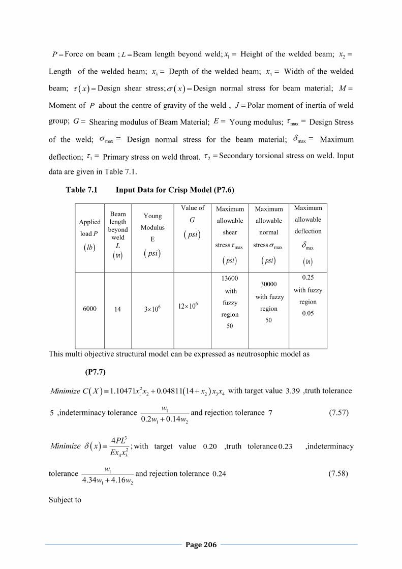
Page 206






of the weld; max Design normal stress for the beam material; max Maximum

deflection; 1 Primary stress on weld throat. 2 Secondary torsional stress on weld. Input

data are given in Table 7.1.


Applied

load P

lb

Beam length beyond

weld L

in

Young

Modulus

E

psi

Value of

G

psi

Maximum

allowable

shear

stress max

psi

Maximum

allowable

normal

stress max

psi

Maximum

allowable

deflection

max

in

6000 14 63 10

612 10

13600

with

fuzzy

region

50

30000

with fuzzy

region

50

0.25

with fuzzy

region

0.05

This multi objective structural model can be expressed as neutrosophic model as

(P7.7)

21 2 2 3 41.10471 0.04811 14Minimize C X x x x x x with target value 3.39 ,truth tolerance

5 ,indeterminacy tolerance 1

1 20.2 0.14w

w wand rejection tolerance 7 (7.57)

3

24 3

4 ;PLMinimize xEx x

with target value 0.20 ,truth tolerance 0.23 ,indeterminacy

tolerance 1

1 24.34 4.16w

w wand rejection tolerance 0.24 (7.58)

Subject to

Page 207

1 max 0;g x x

(7.59)

2 max 0;g x x

(7.60)

3 1 4 0;g x x x

(7.61)

24 1 2 3 4 20.10471 0.04811 14 5 0;g x x x x x x

(7.62)

5 10.125 0;g x x

(7.63)

6 max 0;g x x

(7.64)

7 0;Cg x P P x

(7.65)

1 4 2 30.1 , , , 2.0x x x x

(7.66)

where 2 221 1 2 22

2xxR

; (7.67)

11 22

Px x

; (7.68)

2MRJ

; (7.69)

2

2xM P L

; (7.70)

221 32

4 2x xxR

; (7.71)

221 31 2 2 ;

12 22x xx x xJ

(7.72)

24 3

6 ;PLxx x

(7.73)

3

24 3

4 ;PLxEx x

(7.74)

6 63 4 3

2

4.013 / 361 ;

2 4C

EGx x x EP xL L G

(7.75)

According to GNGP technique using truth, indeterminacy and falsity membership function,

MOWBP (P7.7) can be formulated as

(P7.8)

Model -I

Page 208

,Maximize ,Maximize Minimize (7.76)

21 2 2 3 4

1

1.10471 0.04811 14 3.39 5 1 ,x x x x xw

(7.77)

2 11 2 2 3 4

2 1 2

1.10471 0.04811 14 3.39 ,0.2 0.14

wx x x x xw w w

(7.78)

2 11 2 2 3 4

2 1 2

1.10471 0.04811 14 3.39 5 2 ,0.2 0.14

wx x x x xw w w

(7.79)

21 2 2 3 4

3

71.10471 0.04811 14 3.39 ,x x x x xw

(7.80)

21 2 2 3 41.10471 0.04811 14 3.39,x x x x x

(7.81)

3

24 3 1

4 0.20 0.23 1 ,PLEx x w

(7.82)

31

24 3 2 1 2

4 0.20 ,4.3 4.1

wPLEx x w w w

(7.83)

31

24 3 2 1 2

4 0.20 0.23 0.23 ,4.3 4.1

wPLEx x w w w

(7.84)

3

24 3 3

4 0.240.20 ,PLEx x w

(7.85)

3

24 3

4 0.20,PLEx x

(7.86)

1 2 30 ;w w w

(7.87)

1 2 30, , 0, , 0, ;w w w

(7.88)

1 2 30,1 , 0,1 , 0,1 ;w w w

(7.89)

1 2 30 3;w w w

(7.90)

1 max 0;g x x

(7.91)

2 max 0;g x x

(7.92)

3 1 4 0;g x x x

(7.93)

24 1 2 3 4 20.10471 0.04811 14 5 0;g x x x x x x

(7.94)

Page 209

5 10.125 0;g x x

(7.95)

6 max 0;g x x

(7.96)

7 0;Cg x P P x

(7.97)

1 4 2 30.1 , , , 2.0x x x x

(7.98)

where 2 221 1 2 22

2xxR

; (7.99)

11 22

Px x

; (7.100)

2MRJ

; (7.101)

2

2xM P L

; (7.102)

221 32

4 2x xxR

; (7.103)

221 31 2 2 ;

12 22x xx x xJ

(7.104)

24 3

6 ;PLxx x

(7.105)

3

24 3

4 ;PLxEx x

(7.106)

6 63 4 3

2

4.013 / 361 ;

2 4C

EGx x x EP xL L G

(7.107)


problem (P7.7)based on arithmetic aggregation operator can be formulated as

(P7.9)

Model -II

1 13

Minimize

(7.108)


Page 210


problem (P7.7) based on geometric aggregation operator can be formulated as

(P7.10)

Model -III

3 1 1Minimize

(7.109)


Now these non-linear programming problem Model-I,II,III can be easily solved by an

appropriate mathematical programming to give solution of multi-objective non-linear

programming problem (P7.7) by GNGP approach and the results are shown in Table 7.2.

Table 7.2 Comparison of GNGP Solution of MOWBP (P8.12) based on

Different Aggregation

Methods 1x in 2x in 3x in 4x in

C X

X

Generalized Fuzzy Goal programming(GFGP)

1 0.15w 1.297612

0.9717430

1.693082

1.297612

3.39 0.20

Generalized Intuitionistic

Fuzzy Goal programming(GIFGP)

1 0.15w 3 0.8w 1.297612 0.9717430 1.693082

1.297612

3.39 0.20

Generalized Neutrosophic Goal programming

(GNGP) 1 2 30.4, 0.3, 0.7w w w

1.347503 0.7374240 2

1.347503

3.39 2

Generalized Intuitionistic Fuzzy optimization (GIFGP) based on

Arithmetic Aggregation 1 30.15, 0.8w w

1.297612 0.9717430 1.693082

1.297612

3.39

0.20

Generalized Neutosophic

optimization (GNGP) based on Arithmetic

Aggregation 1 2 30.4, 0.3, 0.7w w w

1.347503 0.7374240 2

1.347503

3.39 0.20

Generalized Intuitionistic Fuzzy optimization (GIFGP) based on

Geometric Aggregation 1 30.15, 0.8w w

1.372 0.697176 2

1.37200

3.39 0.2


optimization (GNGP) based on Geometric

1.372 0.6971 2

1.372

3.39 0.2

Page 211

Aggregation 1 2 30.4, 0.3, 0.7w w w

Here we have got almost same solutions for the different value of 1 2 3, ,w w w in different

aggregation method for objective functions. From Table7.2 it is clear that the cost of welding

and deflection are almost same in fuzzy and intuitionistic fuzzy as well as NSO technique.

Moreover it has been seen that desired value obtained in different aggregation method have

not affected by variation of methods in perspective of welded beam design optimization.

7.4 Conclusion

The research study investigates that NGP can be utilized to optimize a nonlinear welded

beam design problem. The results obtained for different aggregation method of the

undertaken problem show that the best result is achieved using geometric aggregation

method. The concept of NSO technique allows one to define a degree of truth membership,

which is not a complement of degree of falsity; rather, they are independent with degree of

indeterminacy. As we have considered a non-linear welded beam design problem and find out

minimum cost of welding of the structure as well as minimum deflection, the results of this

study may lead to the development of effective neutrosophic technique for solving other

model of nonlinear programming problem in different field.

Page 212

CHAPTER 8

Truss Design Optimization with Imprecise Load and Stress in

Neutrosophic Environment Optimization techniques for structural optimal design, consisting of deterministic optimization and

non-deterministic optimization methods, have been widely used in practice. The former i.e

deterministic optimization aims to search the optimum solution under given constraints without

consideration of uncertainties. However, in so many engineering structures, deterministic optimization

approaches are unable to handle structural performances exhibit variations such as the fluctuation of

external loads, the variation of material properties, e.t.c due to the presence of uncertainties, the so-

called optimum solution obtained may lie in the infeasible region. Thus, so many realistic design-

approaches must be able to deal with the imprecise nature of structures. This type of optimum solution

has been obtained under given reliability constraints, while the later one aims to minimize the

variation of the objective function. Such several non-deterministic structural design optimization

approaches which are reliability-based design optimization (RBDO), solved by D.M Frangopol

et.al[47]and M. Papadrakakis [83], considering structural impreciseness, have been reported in the

literature. Moreover in the practical optimization problems usually more than one objective is

required to be optimized. Generally they are minimum cost, maximum stiffness, minimum

displacement at specific structural nodes, maximum natural frequency of free vibration and optimum

structural strain energy e.t.c. These make it necessary to formulate a multi-objective optimization

problem. The applications of different optimization techniques to structural design have attracted

interest of many researchers. For example Ray Optimization (Kaveh. Et.al [60]), artificial bee colony

algorithm (Sonmez, M.[108]),Particle Swarm Optimization (Perez et. al [84],Kaveh et.al [61] and

Luh,et.al.[70]),genetic Algorithm (Kaveh,et.al[62],Ali.et.al[7],Dede,et.al[42]), meta heuristic

algorithm (Kaveh,A. Motie ,S.Mohammed ,A.,Moslehi,M.[63]),others (Shih, C.j. and

Chang,C.J.[109],Hajela,P. and Shih,C.J.[54]Wang ,D.,Zhang,W.H.and Jiang,J.S.[126],Wang

,D.,Zhang,W.H. and Jiang ,J.S.[127];Kripakaran,P.,Gupta,A. and Baugh Jr,J.W.[64]).Fuzzy as well as

intuitionistic fuzzy optimization, not only help the engineers, especially in structural engineering, to

design and to analyse the systems but also leads to discover fuzzy optimization theory and techniques.

This Fuzzy Set(FS) theory was first introduced by Zadeh[133]. As an extension Intuitionistic Fuzzy

Set(IFS) theory was first introduced by Atanassov[1] .When an imprecise information can not be

expressed by means of conventional FS, IFS plays an important role. In IFS we usually consider

degree of acceptance, and degree of rejection where as we consider only membership function in FS.

A few research work has been done on Intuitionistic Fuzzy Optimization(IFO) in the field of

Page 213

structural optimization. Dey and Roy [35] used IF technique to optimize single objective two bar truss

structural model. A Multi-Objective Intuitionistic Fuzzy Optimization(MOIFO) technique is applied

to optimize three bar truss structural model by Dey and Roy [36] in their paper. When an ill-known

information are represented by IF number which is generalization of fuzzy number expresses the

available information in flexible way considering non-membership functions. Shu [110] applied

Triangular Intuitionistic Fuzzy Number(TIFN) to fault tree analysis on printed board circuit

assembly.P.Grzegorzewski et.al [48], H.B.Mitchell et.al [75],G.Nayagam et.al [78],H.M.Nehi et.al

[79],S.Rezvani et.al [92] used concept of Intuitionistic Fuzzy Number(IFN) in multi-attribute decision

making(MADM) problem. Li[69] proposed a ranking method for TIFN with definition of ratio of

value index to ambiguity index of TIFN in MADM problem as an application. In IFN indeterminate

information is partially lost, as hesitant information is taken in consideration by default. So

indeterminate information should be considered in decision making process. Smarandache

[94]defined Neutrosophic Set(NS) that could handle indeterminate and inconsistent information. In

NS indeterminacy is quantified explicitly with truth membership, indeterminacy membership and

falsity membership function which are independent .Wang et.al [120] define single valued NS which

represents imprecise, incomplete, indeterminate, inconsistent information. Thus taking the universe as

a real line we can develop the concept of single valued neutrosophic number as special case of NS.

These numbers are able to express ill-known quantity with uncertain numerical value in decision

making problem. In this present study, we define generalized single valued triangular neutrosophic

number and total integral value of this number and using a ranking method of single valued

generalized triangular neutrosophic number we solve a multi-objective structural design problem in

neutrosophic environment. In this chapter we have considered three-bar planer truss subjected to a

single load condition .Here the objective functions are weight of the truss and deflection of loaded

joint in test problem and the design variables are the cross-sections of bars with the constraints as

stresses in members. In this chapter we have developed an approach to solve multi-objective structural

design using probabilistic operator in neutrosophic environment. Here total integral values of

Generalized Single Valued Triangular Neutrosophic Numbers(GSVTNN) have been considered for

applied load and stress.

8.1 Multi-Objective Structural Design Formulation

A structural design problem may be considered as a minimization type Multi-Objective Nonlinear

Programming Problem(MONLPP) where weight and deflection of the loaded joint are to be

minimized as objectives and subject to a specified set of stress constraints. The design variables are

cross sectional area of bars. The target of optimization is the identification of the optimum cross-

sectional area of bar so that the structure can achieve its smallest total weight with minimum nodal

displacement, in a given load conditions.

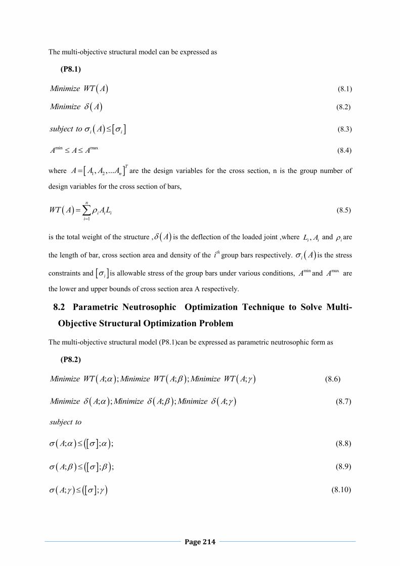
Page 214


(P8.1)

Minimize WT A (8.1)

Minimize A

(8.2)

i isubject to A

(8.3)

min maxA A A (8.4)

where 1 2, ,... TnA A A A are the design variables for the cross section, n is the group number of

design variables for the cross section of bars,

1

n

i i ii

WT A A L

(8.5)

is the total weight of the structure , A is the deflection of the loaded joint ,where ,i iL A and i are

the length of bar, cross section area and density of the thi group bars respectively. i A is the stress

constraints and i is allowable stress of the group bars under various conditions, minA and maxA are

the lower and upper bounds of cross section area A respectively.

8.2 Parametric Neutrosophic Optimization Technique to Solve Multi-

Objective Structural Optimization Problem

The multi-objective structural model (P8.1)can be expressed as parametric neutrosophic form as

(P8.2)

; ; ; ; ;Minimize WT A Minimize WT A Minimize WT A (8.6)

; ; ; ; ;Minimize A Minimize A Minimize A

(8.7)

subject to

; ; ;A

(8.8)

; ; ;A (8.9)

; ;A (8.10)

Page 215

min maxA A A , , 0,1

(8.11)

Where 1 2, ,...., TnA A A A

To solve the MOSOP (P8.1) step 1 of 1.39is used. After that according to step 2 pay-off matrix is

formulated

1 * 1 * 1 * 1 * 1 * 1 * 1

2* 2 * 2 * 2 * 2 * 2 * 2

3* 3 * 3 * 3 * 3 * 3 * 3

* 6 * 6 * 6 * 6 * 66

; ; ; ; ; ;

; ; ; ; ; ;

; ; ; ; ; ;

; ; ; ; ;.... ... ... ... ....

; ; ; ; ;

WT A WT A WT A A A A

A WT A WT A WT A A A AA WT A WT A WT A A A AA

WT A WT A WT A A A A

WT A WT A WT A A AA

* 6

;

...

;A

Here 1 2 6, ,......,A A A are the ideal solution of the objectives

; , ; , ; , ; , ; , ;WT A WT A WT A A A A respectively.

For each objective ; , ; , ; , ; , ; , ;WT A WT A WT A A A A find lower

bound TkL and the upper bound T

kU as

**

;max ; 0 6; , ,

r

TrWT A p

U WT A p r p

(8.12)

**

;min ; 0 6; , ,

r

TrWT A p

L WT A p r p (8.13)

for truth membership of weight functions and

**

;max ; 0 6; , ,

r

TrA p

U A p r p

(8.14)

*

*;

min ; 0 6; , ,r

TrA p

L A p r p

(8.15)

for truth membership of deflection functions

Similarly the upper and lower bounds for indeterminacy and falsity membership of weight objective

function as

* *; ;;

r r

F TWT A p WT A p

U U

(8.16)

* * * *; ; ; ;

;r r r r

F T T TWT A p WT A p WT A p WT A p

L L t U L

(8.17)

* *; ;

;r r

I TWT A p WT A p

L L (8.18)

* * * *; ; ; ;;0 6; , ,

r r r r

I T T TWT A p WT A p WT A p WT A p

U L s U L r p

(8.19)

Page 216

And deflection objective function as

* *; ;,

r r

F TA p A p

U U

(8.20)

* * * *; ; ; ;

;r r r r

F T T TA p A p A p A p

L L t U L

(8.21)

* *; ;,

r r

I TA p A p

L L

(8.22)

* * * *; ; ; ;;0 6; , ,

r r r r

I T T TA p A p A p A p

U L s U L r p

(8.23)


Define truth membership, indeterminacy membership and falsity membership functions for weight

and deflection as follows

*

*

* *

* *

*

;

;

; ; ;; ;

;

1 ;

;; 1 exp ;

0 ;

r

r

r r

r r

r

TWT A p

TWT A p T T

WT A p T T WT A p WT A pWT A p WT A p

TWT A p

if WT A p L

U WT A pT WT A p if L WT A p U

U L

if WT A p U

(8.24)

*

*

* *

* *

*

;

;

; ; ;; ;

;

1 ;

;; exp ;

0 ;

r

r

r r

r r

r

IWT A p

IWT A p I I

WT A p I I WT A p WT A pWT A p WT A p

IWT A p

if WT A p L

U WT A pI WT A p if L WT A p U

U L

if WT A p U

(8.25)

*

* *

*

* *

*

;

; ;

;;

; ;

;

0 ;

1 1 tanh ;2 2 2;

;

1 ;

r

r r

r

r r

r

FWT A p

F FWT A p WT A p

WT A pWT A p

F FWT A p WT A p

FWT A p

if WT A p L

U LWT A p

F WT A p

if L WT A p U

if WT A p U

(8.26)

*

*

* *

* *

*

;

;

; ; ;; ;

;

1 ;

;; 1 exp ;

0 ;

r

r

r r

r r

r

TA p

TA p T T

A p T T A p A pA p A p

TA p

if A p L

U A pT A p if L A p U

U L

if A p U

(8.27)

Page 217

*

*

* *

* *

*

;

;

; ; ;; ;

;

1 ;

;; exp ;

0 ;

r

r

r r

r r

r

IA p

IA p I I

A p I I A p A pA p A p

IA p

if A p L

U A pI A p if L A p U

U L

if A p U

(8.28)

*

* *

*

* *

*

;

; ;

;;

; ;

;

0 ;

1 1 tanh ;2 2 2;

;

1 ;

r

r r

r

r r

r

FA p

F FA p A p

A pA p

F FA p A p

FA p

if A p L

U LA p

F A p

if L A p U

if A p U

(8.29)

Where

*

* *;

; ;

6 ;r

r r

F FWT A pWT A p WT A p

U L

(8.30)

*

* *;

; ;

6 ;r

r r

F FA pA p A p

U L

(8.31)

4 0 6; , ,r p (8.32)

Now NSO method for MONLP problem with probabilistic operator gives a equivalent nonlinear

programming problem as

(P8.3)

; ; ; ;

; ;

; ; ; ;

; ;WT A WT A WT A A

A A

T WT A T WT A T WT A T AMaximize

T A T A

(8.33)

; ; ;

; ; ;

1 ; 1 ; 1 ;

1 ; 1 ; 1 ;

WT A WT A WT A

A A A

I WT A I WT A I WT AMiniimize

I A I A I A

(8.34)

; ; ;

; ; ;

1 ; 1 ; 1 ;

1 ; 1 ; 1 ;

WT A WT A WT A

A A A

F WT A F WT A F WT AMiniimize

F A F A F A

(8.35)

subject to

Page 218

; ; ;0 ; ; ; 3;WT A p WT A p WT A pT WT A p I WT A p F WT A p

(8.36)

; ; ;0 ; ; ; 3;A p A p A pT A p I A p F A p

(8.37)

;A

(8.38)

min maxA A A 0 6; , , ;r p , , 0,1

(8.39)

This crisp nonlinear programming problem can be solved by appropriate mathematical algorithm.

8.3 Numerical Solution of Three Bar Truss Design using Parametric

Neutrosophic Optimization Technique

A well known three bar planer truss( Fig. -8.1) is considered to minimize weight of the



members

Fig.-8.1 Design of the Three-Bar Planar Truss(Shenzhen Stock

Exchange, https://www.e-architect.co.uk,accessed on 18 June 2017)

The multi-objective optimization problem can be stated as follows (P8.4)


1 21

,uLPMinimize A AEA

(8.41)

1 21 2

,2

vLPMinimize A A

E A A

(8.42)

such that

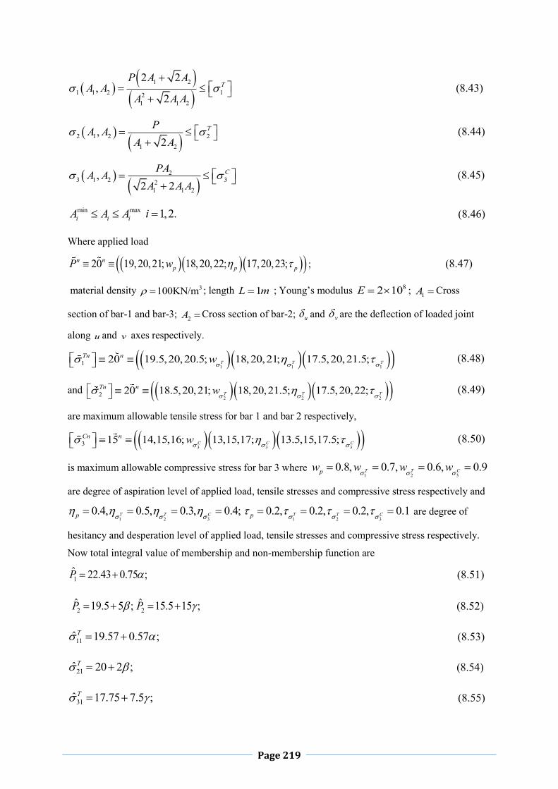
https://www.e-architect.co.uk,accessed/

Page 219

1 2

1 1 2 121 1 2

2 2,

2T

P A AA A

A A A

(8.43)

2 1 2 21 2

,2

TPA AA A

(8.44)

23 1 2 32

1 1 2

,2 2

CPAA AA A A

(8.45)

min max 1,2.i i iA A A i

(8.46)

Where applied load

20 19,20,21; 18,20,22; 17,20,23;n np p pP w ; (8.47)

material density 3100KN/m ; length 1L m ; Young’s modulus 82 10E ; 1A Cross

section of bar-1 and bar-3; 2A Cross section of bar-2; u and v are the deflection of loaded joint

along u and v axes respectively.

1 1 1

1 20 19.5,20,20.5; 18,20,21; 17.5,20,21.5;T T TTn n w

(8.48)

and

2 2 2

2 20 18.5,20,21; 18,20,21.5; 17.5,20,22;T T TTn n w

(8.49)

are maximum allowable tensile stress for bar 1 and bar 2 respectively,

3 3 3

3 15 14,15,16; 13,15,17; 13.5,15,17.5;C C CCn n w

(8.50)

is maximum allowable compressive stress for bar 3 where 1 2 3

0.8, 0.7, 0.6, 0.9T T Cpw w w w

are degree of aspiration level of applied load, tensile stresses and compressive stress respectively and

1 2 30.4, 0.5, 0.3, 0.4;T T Cp

1 2 3

0.2, 0.2, 0.2, 0.1T T Cp are degree of

hesitancy and desperation level of applied load, tensile stresses and compressive stress respectively.

Now total integral value of membership and non-membership function are

1̂ 22.43 0.75 ;P

(8.51)

2̂ 19.5 5 ;P 2̂ 15.5 15 ;P

(8.52)

11ˆ 19.57 0.57 ;T

(8.53)

21ˆ 20 2 ;T

(8.54)

31ˆ 17.75 7.5 ;T

(8.55)

Page 220

12ˆ 19.75 .42 ;T

(8.56)

22ˆ 20.25 3.75 ;T

(8.57)

32ˆ 17 10 ;T

(8.58)

13ˆ 14.55 0.89 ;C

(8.59)

23ˆ 14.5 5 ;C

(8.60)

33ˆ 5 25 ;C

(8.61)

Using total integral values of coefficients, problem (P8.4) can be transformed into

(P8.5)

1 2 1 2, 100 2 2Minimize WT A A A A (8.62)

1 2 81

22.43 0.75, ;

2 10uMinimize A AA

(8.63)

1 2 81

19.5 5, ;

2 10uMinimize A AA

(8.64)

1 2 81

15.5 15, ;

2 10uMinimize A AA

(8.65)

1 2 8

1 2

22.43 0.75, ;

2 10 2vMinimize A A

A A

(8.66)

1 2 8

1 2

19.5 5, ;

2 10 2vMinimize A A

A A

(8.67)

1 2 8

1 2

15.5 15, ;

2 10 2vMinimize A A

A A

(8.68)

such that

1 2

11 1 2 21 1 2

22.43 0.75 2 2, ; 19.57 0.57 ;

2

A AA A

A A A

(8.69)

1 2

21 1 2 21 1 2

19.5 5 2 2, ; 20 2 ;

2

A AA A

A A A

(8.70)

Page 221

1 2

31 1 2 21 1 2

15.5 15 2 2, ; 15.5 15 ;

2

A AA A

A A A

(8.71)

12 1 2

1 2

22.43 0.75, ; 19.75 0.42 ;

2A A

A A

(8.72)

22 1 2

1 2

19.5 5, ; 20.25 3.75 ;

2A A

A A

(8.73)

32 1 2

1 2

15.5 15, ; 17 10 ;

2A A

A A

(8.74)

2

13 1 2 21 1 2

22.43 0.75, ; 19.57 0.57 ;

2 2

AA A

A A A

(8.75)

2

23 1 2 21 1 2

19.5 5, ; 20 2 ;

2 2

AA A

A A A

(8.76)

2

33 1 2 21 1 2

15.5 15, ; 15.5 15 ;

2 2

AA A

A A A

(8.77)

min max 1,2.i i iA A A i , , 0,1

(8.88)

According to step 2 pay-off matrix can be formulated as follows

1 2 1 2 1 2 1 2 1 2 1 2 1 2

1

2

3

4

5

6

7

, , ; , ; , ; , ; , ; , ;

5.994110 12.52100 12.23464 12.15401 7.229002 7.063671 7.0712117.16237 4.486000 4.128718 4.051560 2.419306 2.226623 2.18501215.95051 4.5192

u u u v v vWT A A A A A A A A A A A A A A

AAAAAAA

18 3.90 4.051560 3.048520 2.580241 2.68051319.14214 4.519218 4.135986 3.10 1.908612 1.71318219.14214 4.48600 4.128718 4.051560 1.858162 1.7101719.14214 4.519218 3.90 4.051560 1.90861219.14214 4.519218 4.135986 3.10 1.908612

1.2840621 1.678211

1.615433 1.6782111.713182 1.284062

Here 1 2 1 2 1 2 1 2 1 2 1 2, , , , , ,19.14214, 5.994110 ;F T F T

WT A A WT A A WT A A WT A A WT A A WT A AU U L L

1 2 1 2 1 2 1 2 1 2 1 2, , , , , ,5.994110, 5.994110I T I TWT A A WT A A WT A A WT A A WT A A WT A AL L U L

such that 1 2 1 2, ,0 , 19.14214 5.994110WT A A WT A A ;

1 2 1 2

1 2 1 2 1 2 1 2

, ,, , , ,

6 64, ,WT A A WT A AF F F FWT A A WT A A WT A A WT A AU L U L

Page 222

1 2 1 2 1 2 1 2 1 2 1 2, ; , ; , ; , ; , ; , ;12.52100, 4.486000 ;u u u u u u

F T F TA A A A A A A A A A A AU U L L

1 2 1 2 1 2 1 2 1 2 1 2, ; , ; , ; , ; , ; , ;4.486000, 4.486000u u u u u u

I T I TA A A A A A A A A A A AL L U L

such that

1 2 1 2, ; , ;0 , 12.52100 4.48600u uA A A A

1 2 1 2

1 2 1 2 1 2 1 2

, ; , ;, ; , ; , ; , ;

6 64, ,u u

u u u u

A A A AF F F FA A A A A A A AU L U L

1 2 1 2 1 2 1 2 1 2 1 2, ; , ; , ; , ; , ; , ;12.23464, 3.90 ;u u u u u u


1 2 1 2 1 2 1 2 1 2 1 2, ; , ; , ; , ; , ; , ;3.90, 3.90u u u u u u


such that

1 2 1 2, ; , ;0 , 12.23464 3.90u uA A A A

1 2 1 2

1 2 1 2 1 2 1 2

, ; , ;, ; , ; , ; , ;

6 64, ,u u

u u u u


1 2 1 2 1 2 1 2 1 2 1 2, ; , ; , ; , ; , ; , ;12.15401, 3.1 ;u u u u u u


1 2 1 2 1 2 1 2 1 2 1 2, ; , ; , ; , ; , ; , ;3.10, 3.10u u u u u u


such that

1 2 1 2, ; , ;0 , 12.15401 3.10u uA A A A

1 2 1 2

1 2 1 2 1 2 1 2

, ; , ;, ; , ; , ; , ;

6 64, ,u u

u u u u


1 2 1 2 1 2 1 2 1 2 1 2, ; , ; , ; , ; , ; , ;7.229002, 1.858162 ;v v v v v v


1 2 1 2 1 2 1 2 1 2 1 2, ; , ; , ; , ; , ; , ;1.858162, 1.858162v v v v v v


such that

1 2 1 2, ; , ;0 , 7.229002 1.858162v vA A A A

1 2 1 2

1 2 1 2 1 2 1 2

, ; , ;, ; , ; , ; , ;

6 64, ,v v

v v v v


1 2 1 2 1 2 1 2 1 2 1 2, ; , ; , ; , ; , ; , ;7.063671, 1.615433 ;v v v v v v


1 2 1 2 1 2 1 2 1 2 1 2, ; , ; , ; , ; , ; , ;1.615433, 1.615433v v v v v v


such that

1 2 1 2, ; , ;0 , 7.063671 1.615433v vA A A A

1 2 1 2

1 2 1 2 1 2 1 2

, ; , ;, ; , ; , ; , ;

6 64, ,v v

v v v v


Page 223

1 2 1 2 1 2 1 2 1 2 1 2, ; , ; , ; , ; , ; , ;7.07121, 1.284062 ;v v v v v v


1 2 1 2 1 2 1 2 1 2 1 2, ; , ; , ; , ; , ; , ;1.284062, 1.284062v v v v v v


such that

1 2 1 2, ; , ;0 , 7.07121 1.284062v vA A A A

1 2 1 2

1 2 1 2 1 2 1 2

, ; , ;, ; , ; , ; , ;

6 64, ,v v

v v v v


Here nonlinear truth, indeterminacy and falsity membership function of objectives 1 2, ;WT A A

1 2, ; ;u A A 1 2, ; ;u A A 1 2, ;u A A and 1 2, ; ;v A A 1 2, ; ;v A A 1 2, ;v A A are

defined for 2T as follows

1 2

1 2

1 21 2 1 2,

1 2

1 , 5.994110

19.14214 ,, 1 exp 4 5.994110 , 19.14214

19.14214 5.994110

0 , 19.14214

WT A A

if WT A A

WT A AT WT A A if WT A A

if WT A A

(8.89)

1 2

1 2 1 2

1 2

1 2 ,

1 2

1 2, ,

1 2,

1 2

1 , 5.994110

19.14214 ,exp

, 19.14214 5.994110

5.994110 , 19.14214

0 , 19.14214

WT A A

WT A A WT A A

WT A A

if WT A A

WT A A

I WT A A

if WT A A

if WT A A

(8.90)

1 2

1 2

1 2

1 2

1 2

1 2 ,

,1 2 ,

1 2,

1 2,

1 2

0 , 5.994110

19.14214 5.9941101 1 tanh ,2 2 2,

5.994110 , 19.14214

1 , 19.14214

WT A A

WT A AWT A A

WT A A

WT A A

if WT A A

WT A AF WT A A

if WT A A

if WT A A

(8.91)

1 2

1 2

1 21 2 1 2, ;

1 2

1 , ; 4.48600

12.52100 , ;, ; 1 exp 4 4.48600 , ; 12.52100

12.52100 4.48600

0 , ; 12.52100

u

u

uu uA A

u

if A A

A AT A A if A A

if A A

(8.92)

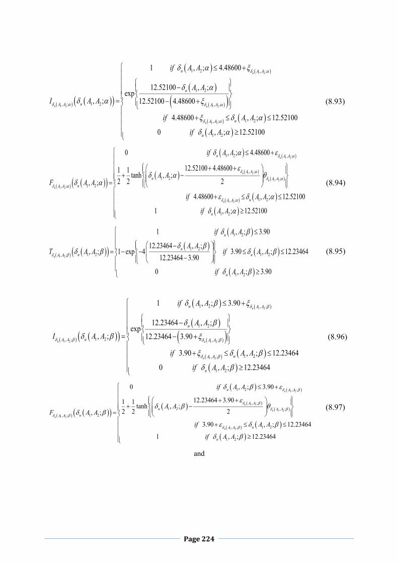
Page 224

1 2

1 2 1 2

1 2

1 2 , ;

1 2

1 2, ; , ;

1 2, ;

1 2

1 , ; 4.48600

12.52100 , ;exp

, ; 12.52100 4.48600

4.48600 , ; 12.52100

0 , ; 12.52100

u

u u

u

u A A

u

uA A A A

uA A

u

if A A

A A

I A A

if A A

if A A

(8.93)

1 2

1 2

1 2

1 2

1 2

1 2 , ;

, ;1 2 , ;

1 2, ;

1 2, ;

1 2

0 , ; 4.48600

12.52100 4.486001 1 tanh , ;2 2 2, ;

4.48600 , ; 12.52100

1 , ; 12.52100

u

u

u

u

u

u A A

A Au A A

uA A

uA A

u

if A A

A AF A A

if A A

if A A

(8.94)

1 2

1 2

1 21 2 1 2, ;

1 2

1 , ; 3.90

12.23464 , ;, ; 1 exp 4 3.90 , ; 12.23464

12.23464 3.90

0 , ; 3.90

u

u

uu uA A

u

if A A

A AT A A if A A

if A A

(8.95)

1 2

1 2 1 2

1 2

1 2 , ;

1 2

1 2, ; , ;

1 2, ;

1 2

1 , ; 3.90

12.23464 , ;exp

, ; 12.23464 3.90

3.90 , ; 12.23464

0 , ; 12.23464

u

u u

u

u A A

u

uA A A A

uA A

u

if A A

A A

I A A

if A A

if A A

(8.96)

1 2

1 2

1 2

1 2

1 2

1 2 , ;

, ;1 2 , ;

1 2, ;

1 2, ;

1 2

0 , ; 3.90

12.23464 3.901 1 tanh , ;2 2 2, ;

3.90 , ; 12.23464

1 , ; 12.23464

u

u

u

u

u

u A A

A Au A A

uA A

uA A

u

if A A

A AF A A

if A A

if A A

(8.97)

and

Page 225

1 2

1 2

1 21 2 1 2, ;

1 2

1 , ; 3.10

12.15401 , ;, ; 1 exp 4 3.10 , ; 12.15401

12.15401 3.10

0 , ; 3.10

u

u

uu uA A

u

if A A

A AT A A if A A

if A A

(8.98)

1 2

1 2 1 2

1 2

1 2 , ;

1 2

1 2, ; , ;

1 2, ;

1 2

1 , ; 3.10

12.15401 , ;exp

, ; 12.15401 3.10

3.10 , ; 12.15401

0 , ; 12.15401

u

u u

u

u A A

u

uA A A A

uA A

u

if A A

A A

I A A

if A A

if A A

(8.99)

1 2

1 2

1 2

1 2

1 2

1 2 , ;

, ;1 2 , ;

1 2, ;

1 2, ;

1 2

0 , ; 3.10

12.15401 3.101 1 tanh , ;2 2 2, ;

3.10 , ; 12.15401

1 , ; 12.15401

u

u

u

u

u

u A A

A Au A A

uA A

uA A

u

if A A

A AF A A

if A A

if A A

(8.100)

1 2

1 2

1 21 2 1 2, ;

1 2

1 , ; 1.858162

7.229002 , ;, ; 1 exp 4 1.858162 , ; 7.229002

7.229002 1.858162

0 , ; 1.858162

v

v

vv vA A

v

if A A

A AT A A if A A

if A A

(8.101)

1 2

1 2 1 2

1 2

1 2 , ;

1 2

1 2, ; , ;

1 2, ;

1 2

1 , ; 1.858162

7.229002 , ;exp

, ; 7.229002 1.858162

1.858162 , ; 7.229002

0 , ; 7.229002

v

v v

v

v A A

v

vA A A A

vA A

v

if A A

A A

I A A

if A A

if A A

(8.102)

1 2

1 2

1 2

1 2

1 2

1 2 , ;

, ;1 2 , ;

1 2, ;

1 2, ;

1 2

0 , ; 1.858162

7.229002 1.8581621 1 tanh , ;2 2 2, ;

1.858162 , ; 7.229002

1 , ; 7.229002

v

v

v

v

v

v A A

A Av A A

vA A

vA A

v

if A A

A AF A A

if A A

if A A

(8.103)

Page 226

1 2

1 2

1 21 2 1 2, ;

1 2

1 , ; 1.615433

7.063671 , ;, ; 1 exp 4 1.615433 , ; 7.063671

7.063671 1.615433

0 , ; 1.615433

v

v

vv vA A

v

if A A

A AT A A if A A

if A A

(8.104)

1 2

1 2 1 2

1 2

1 2 , ;

1 2

1 2, ; , ;

1 2, ;

1 2

1 , ; 1.615433

7.063671 , ;exp

, ; 7.063671 1.615433

1.615433 , ; 7.063671

0 , ; 7.063671

v

v v

v

v A A

v

vA A A A

vA A

v

if A A

A A

I A A

if A A

if A A

(8.105)

1 2

1 2

1 2

1 2

1 2

1 2 , ;

, ;1 2 , ;

1 2, ;

1 2, ;

1 2

0 , ; 1.615433

7.063671 1.6154331 1 tanh , ;2 2 2, ;

1.615433 , ; 7.063671

1 , ; 7.063671

v

v

v

v

v

v A A

A Av A A

vA A

vA A

v

if A A

A AF A A

if A A

if A A

(8.106)

1 2

1 2

1 21 2 1 2, ;

1 2

1 , ; 1.284062

7.07121 , ;, ; 1 exp 4 1.284062 , ; 7.07121

7.07121 1.284062

0 , ; 1.284062

v

v

vv vA A

v

if A A

A AT A A if A A

if A A

(8.107)

1 2

1 2 1 2

1 2

1 2 , ;

1 2

1 2, ; , ;

1 2, ;

1 2

1 , ; 1.284062

7.07121 , ;exp

, ; 7.07121 1.284062

1.284062 , ; 7.07121

0 , ; 7.07121

v

v v

v

v A A

v

vA A A A

vA A

v

if A A

A A

I A A

if A A

if A A

(8.108)

1 2

1 2

1 2

1 2

1 2

1 2 , ;

, ;1 2 , ;

1 2, ;

1 2, ;

1 2

0 , ; 1.284062

7.07121 1.2840621 1 tanh , ;2 2 2, ;

1.284062 , ; 7.07121

1 , ; 7.07121

v

v

v

v

v

v A A

A Av A A

vA A

vA A

v

if A A

A AF A A

if A A

if A A

(8.109)

Page 227

Using fuzzy, Intuitionistic, Neutrosophic Probabilistic Operator for truth; truth, falsity and truth,

indeterminacy , falsity membership function respectively the optimal results of model (P8.5) can be

obtained and is given in Table 8.1.

Table 8.1 Optimal weight and deflection for 1 2 1 2, ,, 1.3;WT A A WT A A

1 2 1 2, ; , ;, 0.8;u uA A A A

1 2 1 2, ; , ;, 0.83;u uA A A A

1 2 1 2, ; , ;, 0.9;u uA A A A

1 2 1 2, ; , ;, 0.53;v vA A A A

1 2 1 2, ; , ;, 0.54;v vA A A A

1 2 1 2, ; , ;, 0.57;v vA A A A

Method * 4 21 10A m * 4 2

2 10A m * 210WT KN * 710u m * 710v m

Fuzzy Max-

Min Operator

2.425445

1.568392

8.428587 0.5830738

0.3045585

Fuzzy

Probabilistic

operator

2.299305

4.006269 10.50968 8.698282 2.510978

Intuitionistic

Probabilistic

Operator

1.495007 2.604875 6.833394 13.37785 3.861852

Neutrosophic

Probabilistic

Operator

4.903401 4.807390 18.67630 4.078801 1.709098

From the Table 8.1.we may arrive to the conclusion that the weight is minimized when we have

solved the model in intuitionistic optimization technique. As an explanation we can say in IFO we

usually minimize non membership functions and maximize membership functions simultaneously. So

it gives better result compare to FO where we only consider membership function for minimization.

But as degree of acceptance is partially included in hesitancy and we minimize it in NSO it has given

higher value than the result obtained in intuitionistic optimization.

8.4 Conclusion

In this chapter we have proposed a method to solve multi-objective structural model in neutrosophic

environment. Here generalized neutrosophic number has been considered for applied load and stress

parameter. The said model is solved by neutrosophic probabilistic operator and result is compared

with fuzzy as well as intuitionistic probabilistic operator. The weight of the truss is more optimized by

intuitionistic optimization technique. The main advantage of the described method is that it allows us

Page 228

to overcome the actual limitations in a problem where impreciseness of supplied data are involved

during the specification of the objectives. This approximation method can be applied to optimize

different models in various fields of engineering and sciences.

Page 229

CHAPTER 9

Optimization of Welded Beam with Imprecise Load and Stress by Parameterized Neutrosophic Optimization Technique

Welding is a process of joining metallic parts by heating to a suitable temperature with or

without the application of pressure. In this chapter we have investigated a problem which is a

simplified example of many complex design issues arising in structural engineering. The

problem is dealing with designing the form of steel beams and with connecting them to form

complex structure like bridges, buildings etc. The problem of designing an optimum welded

beam consists of dimensioning a welded steel beam and the welding length so as to minimize

its cost subject to constraints on sheer stress, bending stress in the beam, buckling load on the

bar, the end the deflection on the beam and the side constraints. Most importantly the design

of welded beam should preferably be economical and durable one. Since decades,

deterministic optimization has been widely used in practice for optimizing welded connection

design. These include mathematical traditional optimization algorithms (Ragsdell & Phillips

[90]) ,GA-based methods (Deb [40], Deb [37], Coello [14], Coello [25]), particle swarm

optimization (Reddy [59]), harmony search method (Lee & Geem [67]), and Big-Bang Big-

Crunch (BB-BC) algorithm (O. Hasançebi, [65]), subset simulation (Li [73]), improved

harmony search algorithm (Mahadavi [72]), as methods used to solve this problem. All these

deterministic optimizations aim to search the optimum solution under given constraints

without consideration of uncertainties. So, while a deterministic optimization approach is

unable to handle structural performances such as imprecise stresses and deflection etc. due to

the presence of impreciseness, to get rid of such problem Fuzzy Set(FS)(Zadeh, [133]),

Intuitionistic Fuzzy Set(IFS) (Atanassov,[1]) Neutrosophic Set(NS)(Smarandache [99]) play

great roles. In IFS theory we usually consider degree of acceptance, and degree of rejection

where as we consider only membership function in FS. Sarkar [104] optimize two bar truss

design with imprecise load and stress in Intuitionistic Fuzzy(IF) environment calculating total

integral values of Triangular Intuitionistic Fuzzy Number(TIFN). Shu [108] applied TIFN to

fault tree analysis on printed board circuit assembly .P.Grzegorzewski et.al [48],H.B.Mitchell

et.al [75],G.Nayagam et.al [78],H.M.Nehi et.al [79],S.Rezvani et.al [92] have been employed

concept of

Page 230

Intuitionistic Fuzzy Number (IFN) in Multi-Attribute Decision Making (MADM) problem

.So indeterminate information should be considered in decision making process. A few

research work has been done on Neutrosophic Optimization (NSO) in the field of structural

optimization. So to deal with different impreciseness on load, stresses and deflection, we

have been motivated to incorporate the concept of Neutrosophic Number(NN) in this

problem, and have developed NSO algorithm to optimize the optimum design in imprecise

environment. In IFN indeterminate information is partially lost, as hesitant information is

taken in consideration by default. So indeterminate information should be considered in

decision making process. Smarandache [94] defined neutrosophic set that could handle

indeterminate and inconsistent information. In neutrosophic sets indeterminacy is quantified

explicitly with truth membership, indeterminacy membership and falsity membership

function which are independent. Wang et.al [120] define Single Valued Neutrosophic

Set(SVNS) which represents imprecise, incomplete, indeterminate, inconsistent information.

Thus taking the universe as a real line we can develop the concept of single valued

neutrosophic number as special case of neutrosophic sets. These numbers are able to express

ill-known quantity with uncertain numerical value in decision making problem.We define

generalized triangular neutrosophic number and nearest interval approximation of this

number. Then using parametric interval valued function for approximated interval number of

NN we solve WBD problem in neutrosophic environment .This paper develops optimization

algorithm using max-min operator in neutrosophic environment to optimize the cost of

welding, while the maximum shear stress in the weld group, maximum bending stress in the

beam, and buckling load of the beam and deflection at the tip of a welded steel beam have

been considered as constraints. Here parametric interval valued function of Generalized

Triangular Neutrosophic Number(GTNN) have been considered for applied load , stress and

deflection .The present study investigates computational algorithm for solving single-

objective nonlinear programming problem by parametric NSO approach.

9.1 General Formulation of Single-Objective Welded Beam Design

In sizing optimization problems, the aim is to minimize single objective function, usually the

cost of the structure under certain behavioural constraints which are displacement or stresses.

The design variables are most frequently chosen to be dimensions of the height, length, depth

and width of the structures. Due to fabrications limitations the design variables are not

Page 231

continuous but discrete for belongingness of cross-sections to a certain set. A discrete


(P9.1)


, 1,2,...,i isubject to X i m

(9.2)

, 1,2,...,djX R j n

(9.3)

where ( )C X represents cost function, i X is the behavioural constraints and i X

denotes the maximum allowable value , ‘m’ and ‘n’ are the number of constraints and design

variables respectively. A given set of discrete value is expressed by dR and in this chapter

objective function is taken as

1 1

mTtn

t nt n

C X c x

(9.4)


i iX with allowable tolerance 0i for 1,2,....,i m (9.5)

The deflection of the structure as follows

maxX with allowable tolerance 0max (9.6)


the number of structural element, i and 0i 0

max are the thi stress , allowable stress and

allowable deflection respectively.

9.2 NSO Technique to Optimize Parametric Single-Objective Welded

Beam Design(SOWBD)

The parametric WBD problem can be formulated as

(P9.2)

( ; )Minimize C X s (9.7)

; , 1,2,..,i isubject to X s s i m (9.8)

Page 232

, 1,2,.....,djX R j n

(9.9)

0; 0,1X s

(9.10)

where ( ; )C X s represents cost function, ;i X s is the behavioural constraints and

;i X s denotes the maximum allowable value , ‘m’ and ‘n’ are the number of constraints

and design variables respectively. A given set of discrete value is expressed by dR and in this

chapter objective function is taken as

1 1

;mT

tnt n

t nC X s c s x

(9.11)


; ni iX s s with allowable tolerance 0

i s for 1,2,....,i m (9.12)

The deflection of the structure as follows

max; nX s s with allowable tolerance 0max s (9.13)


the number of structural element, i and 0i s 0

max s are the thi stress , allowable stress and

allowable deflection respectively.

To solve the SOWBP (P9.2), step 1 of 1.40 is used and let ; ; ;, ,T I F

C X s C X s C X sU U U be the

upper bounds of truth, indeterminacy , falsity function for the objective respectively and

; ; ;, ,T I FC X s C X s C X sL L L be the lower bound of truth, indeterminacy, falsity membership

functions of objective respectively then

1 2; max ; , ; ,T

C X sU C X s C X s

(9.14)

1 2; min ; , ; ,T

f x sL C X s C X s (9.15)

; ; ,F TC X s C X sU U

(9.16)

; ; ; ; ; ;0F T T TC X s C X s C X s C X s C X s C X sL L where U L (9.17)

; ; ,I TC X s C X sL L

(9.18)

; ; ; ; ; ;0I T T TC X s C X s C X s C X s C X s C X sU L where U L (9.19)

Page 233

Let the linear membership function for objective be

;

;; ; ;

; ;

;

1 ;

;; ;

0 ;

TC X s

TC X s T T

C X s C X s C X sT TC X s C X s

TC X s

if C X s L

U C X sT C X s if L C X s U

U L

if C X s U

(9.20)

;

;; ; ;

; ;

;

1 ;

;; ;

0 ;

IC X s

IC X s I I

C X s C X s C X sI IC X s C X s

IC X s

if C X s L

U C X sI C X s if L C X s U

U L

if C X s U

(9.21)

;

;; ; ;

; ;

;

0 ;

;; ;

1 ;

FC X s

FC X s F F

C X s C X s C X sF FC X s C X s

FC X s

if C X s L

C X s LF C X s if L C X s U

U L

if C X s U

(9.22)

and constraints be

00

; 0

0

1 ;

;; ;

0 ;

j

j j

j j jj j j j jg x s

j

j j

if g x s b s

b s b s g x sT g x s if b s g x s b s b s

b s

if g x s b s

(9.23)

;

; ;;

;

1 ;

;; ;

0 ;

j

j j

j

j

j j

j jg x sj j j jg x s g x s

g x s

j j g x s

if g x s b s

b s g x sI g x s if b s g x s b s

if g x s b s

(9.24)

;

; 0; ;0

;

0

0 ;

;; ;

1 ;

j

j

j j

j

j j g x s

j j g x sj j j j jg x s g x s

j g x s

j j j

if g x s b s

g x s b sF g x s if b s g x s b s b s

b s

if g x s b s b s

(9.25)

Page 234

where and for

0; ;1,2,....., 0 ,

j j jg x s g x sj m b

where and for 0;; ; ; ; ,0

jj j j j jg X sg X s X s or X s or X s b s

then parametric NSO problem can be formulated as [107],i.e

(P9.3)

Maximize (9.26)

; ; ;; . ;T T TC X s C X s C X ssuch that C X s U L U

(9.27)

; ; ;; . ;I I IC X s C X s C X sC X s U L U

(9.28)

; ; ;; . ;F F FC X s C X s C X sC X s U L L

(9.29)

; ; ;; . ;j j j

T T Tj g x s g x s g x sg x s U L U

(9.30)

; ; ;; . ;j j j

I I Ij g x s g x s g x sg x s U L U

(9.31)

; ; ;; . ;j j j

F F Fj g x s g x s g x sg x s U L L

(9.32)

3; ; ; , , 0,1 ; (9.33)

0, 0,1x s

(9.34)

where 0;; ; ; ; ,0

jj j j j jg X sg X s X s or X s or X s b s

All these crisp nonlinear programming problems (P9.3) can be solved by appropriate

mathematical algorithm.

9.3 Numerical Solution of Parametric Welded Beam Design Problem by

NSO Technique

A welded beam (Ragsdell and Philips 1976,Fig.-9.1) has to be designed at minimum cost

whose constraints are shear stress in weld ,bending stress in the beam ,buckling

load on the bar P ,and deflection of the beam .The design variables are

1

2

3

4

x hx lx tx b

where

Page 235

h is the weld size, l is the length of the weld , t is the depth of the welded beam, b is the

width of the welded beam.

Fig.-9.1 Design of the Welded Beam(http://www.spantec.com.au,accessed

on 20June 2017)


(P9.4)


Such that

1 max 0;g x x

(9.36)

2 max 0;g x x

(9.37)

3 1 4 0;g x x x

(9.38)

2

4 1 2 3 4 20.10471 0.04811 14 5 0;g x x x x x x

(9.39)

5 10.125 0;g x x

(9.40)

6 max 0;g x x

(9.41)

7 0;Cg x P P x

(9.42)

1 4 2 30.1 , , , 2.0x x x x

where 2 221 1 2 22

2xxR

; (9.43)

11 22

Px x

; (9.44)

http://www.spantec.com.au,accessed/

Page 236

2MRJ

; (9.45)

2

2xM P L

; (9.46)

221 32

4 2x xxR

; (9.47)

221 31 2 2 ;

12 22x xx x xJ

(9.48)

24 3

6 ;PLxx x

(9.49)

3

24 3

4 ;PLxEx x

(9.50)

6 63 4 3

2

4.013 / 361 ;

2 4C

EGx x x EP xL L G

(9.51)







1 Primary stress on weld throat. 2 Secondary torsional stress on weld. Input data are

given in Table 10.1and Table 10.2.


Applied load P lb

Beam length beyond weld

L in

Young

Modulus

E psi

Value

of

G psi

Page 237

6000

5580,6000,6100;

5575,5590,6110;

5570,5585,6120;

p

p

p

w

14 63 10

612 10

Table 9.2 Input Data For Crisp Model (P9.4)

Maximum allowable

shear

stress max psi

Maximum allowable

deflection max in

Maximum allowable

normal stress max psi

13550

13520,13550,13580;

13510,13540,13570;

13500,13530,13560;

w

Maximum allowable

value

1

1

1

13600

13580,13600,13610;

13575,13590,13615;

13570,13585,136120;

w

0.25

0.22,0.25,0.26;

0.21,0.24,0.27;

0.20,0.23,0.28;

w

Maximum allowable

value

1

1

1

0.26

0.23,0.26,0.27;

0.22,0.25,0.28;

0.21,0.26,0.29;

w

3000

2980,3000,3030;

2975,2990,3020;

2970,2985,3010;

w

Maximum allowable

value

1

1

1

3100

3070,3100,3130;

3060,3090,3120;

3050,3080,3110;

w

where , , ,pw w w w and 1 1 1, , ,pw w w w are degree of truth membership or aspiration level

and maximum degree of truth membership or aspiration level; , , ,p ; 1 1 1, , ,p are

degree of indeterminacy and maximum degree of indeterminacy and , , ,p and

1 1 1, , ,p are degree of falsity and maximum degree of falsity or desperation level of

applied load, normal stress ,deflection and allowable shear stress respectively .

Now parameterized value of interval valued function can be calculated as 1

70 2.5 2.5 16.67 86.67 89.17ˆ 5575 6110 ;s s

a a a a a a

Pw w

(9.52)

Page 238

1max 5 5 5 1.67 5 5ˆ 13510 13570 ;

s s

a a a a a aw w

(9.53)

Allowable value of max̂

1max1

3.33 2.5 2.5 1.67 4.17 5.83ˆ 13575 13615 ;s s

a a a a a aw w

(9.54)

1max 0.005 0.005 0.005 0.001 0.005 0.008ˆ 0.21 0.27 ;

s s

a a a a a aw w

(9.55)


1max

10.005 0.005 0.005 0.001 0.005 0.008ˆ 0.22 0.28 ;

s s

a a a a a aw w

(9.56)

1max 3.33 2.5 2.5 1.67 5 7.5ˆ 2975 3020 ;

s s

a a a a a aw w

(9.57)


1max1

5 5 5 1.67 5 8.83ˆ 3060 3120 ;s s

a a a a a aw w

(9.58)

Table 9.3 The Upper and Lower Value of Objective(P9.4) for Different Values of

w Pessimistic Value of s

The pessimistic value of s=0.2

Aspiration level ,uncertainty level and

desperation level

1 1 1

p

p

w w w w

w w w w w

1 1 1

p

1 1 1

p

0.3w

0.5w

0.7w

Page 239

Upper and lower value of

objective

0.1419847,TC XL

0.1425069T

C XU

0.1387723,T

C XL

0.1393634T

C XU

0.1374016,TC XL

0.1380209T

C XU

Table 9.4 The Upper and Lower Value of Objective (P9.4)for Different Values of

w ,Moderate Value of s



desperation level

1 1 1

p

p

w w w w

w w w w w

1 1 1

p

1 1 1

p

0.3w

0.5w

0.7w


objective

0.1485833,TC XL

0.1491453T

C XU

0.1444032,T

C XL

0.1450005T

C XU

0.1426218,TC XL

0.1432331T

C XU

Table 9.5 The Upper and Lower Value of Objective(P9.4) for Different

Values of w Optimistic Value of s



desperation level

1 1 1

p

p

w w w w

w w w w w

1 1 1

p

0.3w

0.5w

0.7w

Page 240

1 1 1

p


objective

0.1555725TC XL

0.1561771T

C XU

0.1503266T

C XL

0.1509290T

C XU

0.1480966TC XL

0.1486975T

C XU

Now using truth, indeterminacy and falsity membership function as mentioned in section 10.4

neutrosophic optimization problem can be formulated as similar as (P9.4) and solving this

optimal for different values of , , ,s w ,design variables and objective functions can be

obtained as follows.

Table 9.6 The Optimum Values of Design Variables(P9.4) for Different Values of

, ,w and 0.2s

Value of ,i i .Aspiration level

,uncertainty level and desperation level

1 1 1

p

p

w w w w

w w w w w

1 1 1

p

1 1 1

p

0.3w

0.1i

T Ti iU L

0.1i

T Ti iU L

0.5w

0.1i

T Ti iU L

0.1i

T Ti iU L

0.7w

0.1i

T Ti iU L

0.1i

T Ti iU L

1( )x in 0.3415895 0.3389869 0.3378618

2 ( )x in 0.9535080 0.9463785 0.9433100

3( )x in 2 2 2

4 ( )x in 1.089426 1.080890 1.077210

$C X 0.1420369 0.1388314 0.1374635

Where i iU and L are upper and lower bound of respective objective and The Optimum

constraints.

Page 241

Table 9.7 The Optimum Values of Design Variables(P9.4) for Different

Values of , ,w and 0.5s

Value of ,i i . Aspiration level

uncertainty level and desperation level

1 1 1

p

p

w w w w

w w w w w

1 1 1

p

1 1 1

p

0.3w

0.1i

T Ti iU L

0.1i

T Ti iU L

0.5w

0.1i

T Ti iU L

0.1i

T Ti iU L

0.7w

0.1i

T Ti iU L

0.1i

T Ti iU L

1( )x in 0.3422657 0.3396719 0.3385506

2 ( )x in 0.9552806 0.9481638 0.9451009

3( )x in 2 2 2

4 ( )x in 1.091979 1.083465 1.079794

$C X 0.1486395 0.1444629 0.1426829

Where i iU and L are upper and lower bound of respective objective and constraints.

Table 9.8 The Optimum Values of Design Variables(P9.4) for Different Values of

, ,w and 0.8s

Value of ,i i . Aspiration level

,uncertainty level and desperation level

1 1 1

p

p

w w w w

w w w w w

1 1 1

p

0.3w

0.1i

T Ti iU L

0.1i

T Ti iU L

0.5w

0.1i

T Ti iU L

0.1i

T Ti iU L

0.7w

0.1i

T Ti iU L

0.1i

T Ti iU L

Page 242

1 1 1

p

1( )x in 0.3429429 0.3403578 0.3392404

2 ( )x in 0.9570581 0.9499542 0.9468969

3( )x in 2 2 2

4 ( )x in 1.094538 1.086046 1.082384

$C X 0.1556330 0.1503868 0.1503868

Where i iU and L are upper and lower bound of respective objective and constraints

From the above results it is clear that whenever we chose 0.7w and 0.2s ,

the of cost welding is minimum most. Also it has been observed that cost of welding is

decreased by higher value of aspiration level, uncertainty level and desperation level for a

particular value of parameter ‘s’.

9.4 Conclusion

In this chapter we have proposed a method to solve WBD in fully neutrosophic

environment. Here GNN has been considered for deflection and stress parameter. The said

model is solved by Single Objective Parametric Neutrosophic Optimization (SOPNSO)

technique and result is calculated for different parameter. The main advantage of the

described method is that it allows us to overcome the actual limitations in a problem where

impreciseness of supplied data is involved during the specification of the objectives. This

approximation method can be applied to optimize different models in various fields of

engineering and sciences.

Page 243

CHAPTER 10

Optimization of Thickness of Jointed Plain Concrete Pavement

Using Neutrosophic Optimization Technique

Highway construction agencies throughout the globe chasing accelerating demands on

durable undowelled Jointed Plain Concrete Pavement (JPCP) due to scanty of rehabilitation

of the same . Since decades, different design methods had been developed by various

organizations which suit their locale and fix the depth criteria of the JPCP along with other

parameters by satisfying the standard code of practice but none of them tries to optimize the

design thickness of the same (Hadi and Arfiadi, [53]). However a few approaches designed

such thickness of cited pavement by considering traffic overloading condition, its fatigue life

and the fluctuation of ambient temperature effect individually (Maser et al., [74];Ramsamooj

[91];Levenberg, [68]). But during service life of such pavement, the traffic loads and adverse

environmental effect would deteriorate its joints and ultimately its foundation. Therefore

optimization of such rigid pavement is become essential considering multiple decision

making criteria as stated above to make it more durable.

Several design methods e.g. AASHTO, PCA, Crop of Engineers of the US army iteration

method etc. are available to determine the thickness of JPCP. However all such methods

follow numerous monographs, tables and charts to do the same and abiding by certain loop of

algorithm in the cited iteration process to find an effective thickness of such pavement. But

most of the time, designers stop the cited procedure even after two or three trials which yields

safe but unnecessarily less economical thick rigid pavement (Hadi and Arfiadi, [53]).

However lots of efforts had been made to get rid of from such problem but optimization on

the same subject has rarely found. Moreover, finite element method (Davids, [40]) and

genetic Algorithm (Hadi and Arfiadi, [53]) type of crisp optimization method had been

applied on the cited subject, where the values of the input parameters were obtained from

experimental data in laboratory scale. While the above cited standards has already ranged the

magnitude of those parameters in between maximum to the minimum value. Therefore,

designer get confused to select those input parameters from such ranges which yield three key

governing factors i.e. degree of acceptance, rejection and hesitancy that attributes the

Page 244

necessity of neutrosophic fuzzy set (Das et al., [39]; Sarkar et al., [107]). Meanwhile, Wang

et.al [120] presented such set as Single Valued Neutrosophic Set (SVNS) as it comprised of

generalized classic set, Fuzzy set, interval valued fuzzy set, Intuitionistic Fuzzy Set and para

consistent set respectively.

As application of SVNS optimization method is rare in rigid pavement design; hence it is

used to minimize the thickness of the pavement by considering cumulative fatigue life and

deflection as constraints respectively. However the factors governing of former constraints

are axel loads, pavement thickness, modulus of elasticity of cement concrete, subgrade

modulus, poisson’s ratio, load contact area, annual rate of growth of commercial traffic,

number of axel per day, radius of relative stiffness and design period respectively. While, the

later constraint includes radius of load contact area, subgrade modulus, radius of relative

stiffness and single as well as tandem axel loads respectively. Besides that, in this effort

flexibility has been given in number of axel per day in fatigue life constraint only; hence

cumulative vehicle per day (CVPD) becomes imprecise in nature so that it can be considered

as neutrosophic set to from truth, indeterminacy and falsity membership functions. Ultimately

neutrosophic optimization technique can be applied on the basis of cited membership

functions and outcome of such Nonlinear Optimum Pavement Design (NLOPD) tries to

provide the minimum thickness for varying subgrade modulus of soil.

10.1 Formulation for Optimum JPCP Design

The first step of formulation of JPCP is to formulate the pavement optimization problem by

defining objective function (minimum thickness) and the constraints (fatigue life consumed,

deflection and corner stress due to single and tandem axle) that control the solution.

Fig.-10.1 Construction and Fatigue Failure of JPCP(http://www.escsi.org,

Page 245

http://c3sinc.com,accessed on 20 June 2017)

10.1.1 Design input parameters

The input parameters that influence the design are Poisson ratio , Load due to single axle

1P , Load due to tandem axle 2P , Modulus of elasticity of concrete E , Modulus of

subgrade reaction k , Radius of load contact areas assumed circular a , Initial number of

axles per day in the year A , Design period in year n , Annual rate of growth of commercial

traffic r , Limiting value of deflection due to single axle 1d , Limiting value of deflection

due to tandem axle 2d , Flexural strength of concrete fS ,

10.1.2 Design method

For determining optimum thickness of JPCP ,a crisp mathematical model has been

formulated. Here Thickness of Slab (TS) has been minimized subjected to a specified set of

constraints (P11.1) .Here the optimum design is

(P10.1)


subject to

2 3.268 2 6.536 2


(10.2)

2

1 22 1 2 1 2

365 1 1 0.25, , , , 2 23.47

0.25 0.0828


r

(10.3)

112

0.431, 1 0.82SALP aD k l d

kl l

(10.4)

222

0.431, 1 0.82TALP aD k l d

kl l

(10.5)

1.2

12

3 21CSAL f

P aS h Sh l

(10.6)

http://c3sinc.com,accessed/

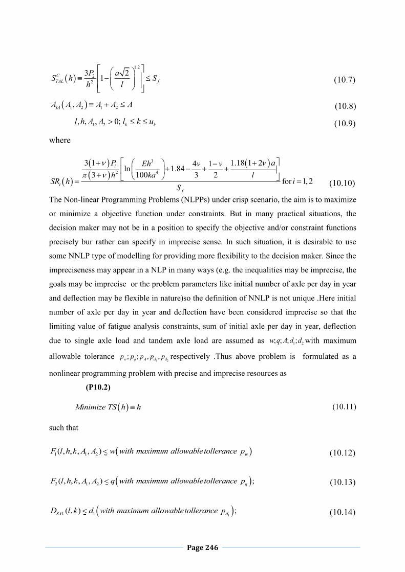
Page 246

1.2

22

3 21CTAL f

P aS h Sh l

(10.7)

1 2 1 2,IAA A A A A A (10.8)

1 2, , , 0;l h A A k kl k u (10.9)

where

3

2 4

3 1 1.18 1 24 1ln 1.843 100 3 2

i

if

P aEh v vh ka l

SR hS

for 1,2i (10.10)

The Non-linear Programming Problems (NLPPs) under crisp scenario, the aim is to maximize

or minimize a objective function under constraints. But in many practical situations, the

decision maker may not be in a position to specify the objective and/or constraint functions

precisely bur rather can specify in imprecise sense. In such situation, it is desirable to use

some NNLP type of modelling for providing more flexibility to the decision maker. Since the

impreciseness may appear in a NLP in many ways (e.g. the inequalities may be imprecise, the

goals may be imprecise or the problem parameters like initial number of axle per day in year

and deflection may be flexible in nature)so the definition of NNLP is not unique .Here initial

number of axle per day in year and deflection have been considered imprecise so that the

limiting value of fatigue analysis constraints, sum of initial axle per day in year, deflection

due to single axle load and tandem axle load are assumed as 1 2; ; ; ;w q A d d with maximum

allowable tolerance 1 2

; ; , ,w q A d dp p p p p respectively .Thus above problem is formulated as a

nonlinear programming problem with precise and imprecise resources as

(P10.2)


such that

1 1 2( , , , , ) wF l h k A A w with maximum allowabletollerance p (10.12)

2 1 2( , , , , ) ;qF l h k A A q with maximum allowabletollerance p (10.13)

11( , ) ;SAL dD l k d with maximum allowabletollerance p

(10.14)

Page 247

22( , ) ;TAL dD l k d with maximum allowabletollerance p

(10.15)

;CSAL fS h S

(10.16)

CTAL fS h S

(10.17)

1 2,IAA A A A ( )Awith maximum allowable tollerance p (10.18)

1 2, , , , 0, k kl h t A A l k u (10.19)

Where kl and ku are the lower and upper limit of k respectively

2 3.2682

1 1 2 1 2, , , , 365 1 1 0.25 0.4325 0.4325F l h k A A r SR SR (10.20)

2 6.536 2

1 2

0.5 4.2577 rw

A A

(10.21)

2

1 22 1 2

365 1 1 0.25, , , , 2 23.47;

0.5 0.0828

r SR SRF l h k A A Logr

(10.22)

1 2q Log A A (10.23)

12

0.431, 1 0.82SALP aD k l

kl l

(10.24)

22

0.431, 1 0.82TALP aD k l

kl l

(10.25)

1 2 1 2,IAA A A A A (10.26)

3

2 4

3 1 1.18 1 24 1ln 1.843 100 3 2

i

if

v P v aEh v vv h ka l

SR hS

Page 248

for i=1,2 (10.27)

To solve above nonlinear programming problem (P10.2) we have used Neutrosophic

Optimization Technique

10.2 Neutrosophic Optimization

In conventional optimization problems, it is assumed that the decision maker is sure about the

precise values of data involved in the model. But in real world applications all the parameters

and goals (objective goals ,constraint goals etc.) of the optimization problems may not be

known precisely due to uncontrollable factors. Such type of imprecise parameters and goals

are represented by fuzzy set theory (Zadeh [133])

Actually, a decision maker may assume that an object belongs to a set to a certain degree, but

it is possible that he is not sure about it. In other words, there may be uncertainty about the

membership degree. The main premise is that the parameters’ demands across the problem

are uncertain. So, they are known to fall within a prescribed uncertainty set with some

attributed degree. In fuzzy set theory, there is no means to incorporate this hesitation in the

membership degree. To incorporate the uncertainty in the membership degree, intuitionistic

fuzzy sets (IFSs) proposed by Atanassov [1] is an extension of fuzzy set theory.In

intuitionistic fuzzy set theory along with degree of membership a degree of non-menbership

is usually considered to express ill-know quantity. This degree of membership and non-

memship functions are so defined as they are independent to each other and sum of them is

less or equal to one. So IFS is playing an important role in decision making under uncertainty

and has gained popularity in recent years. However an application of the IFSs to optimization

problems introduced by Angelov [4] His technique is based on maximizing the degree of

membership, minimizing the degree of non-membership and the crisp model is formulated

using the IF aggregation operator.

Now the fact is that in IFS indeterminate information is partially lost ,as hesitant information

is taken in consideration by default. So indeterminate information should be considered in

decision making process. Smarandache [94] defined NS that could handle indeterminate and

inconsistent information. In neutrosophic sets indeterminacy is quantified explicitly with

truth membership, indeterminacy membership and falsity membership function which are

independent .Wang et.al [120] define SVNS which represents imprecise, incomplete,

indeterminate, inconsistent information. Thus taking the universe as a real line we can

develop the concept of single valued NS as special case of NS. These set is able to express

Page 249

ill-known quantity with uncertain numerical value in decision making problem. It help more

adequately to represent situations where decision makers abstain from expressing their

assessments. In this way NS provide a richer tool to grasp impression and ambiguity than the

conventional fuzzy as well as IFS. These characteristics of neutrosophic set led to the

extension of optimization methods in Neutrosophic Environment (NSE).

Besides It has been seen that the current research on fuzzy mathematical programming is

limited to the range of linear programming introduced by Ziemmermann[136] . He showed

that the solutions of Fuzzy Linear Programming Problems (FLPPs) are always efficient. The

most common approach for solving fuzzy linear programming problem is to change it into

corresponding crisp linear programming problem. But practically there exist many fuzzy and

intuitionistic fuzzy nonlinear structural , pavement design problems in the field of civil

engineering. These problems cannot be modelled as a linear form and solved by traditional

techniques due to presence of imprecise information.

So, the research on modelling and optimization for nonlinear programming under fuzzy

intuitionistic fuzzy and neutrosophic environment are not only necessary in the fuzzy

optimization theory but also has great and wide value in application to structural engineering

problems of conflicting and imprecise nature. So following nonlinear neutrosophic

optimization technique ( Sarkar et.al.[100]) the proposed nonlinear JPCP (P10.1) for the first

time ever being solved with LINGO 11.0 in neutrosophic environment in this chapter and

literature. LINGO 11.0 is a comprehensive tool designed to make building and solving

mathematical optimization models easier and more efficient. LINGO provides a completely

integrated package that includes a powerful language for expressing optimization models,

a full-featured environment for building and editing problems, and a set of fast built-in

solvers capable of efficiently solving most classes of optimization models. However the

outcome of this investigation has been furnished in the following flowchart by incorporating

all the essential parameters associated with the pavement design. In this regard it can be cited

that fuzzy, IF and neutrosophic NLP are rarely involved in literature and Das et.al [25]

developed neutrosophic NLP with numerical example and application of real life problem

recently.

Page 250

Fig.-10.2 Flow Chart for Work Plan of The JPCP Design Study

Minimization of thickness of Slab subject to

Minimization of thickness of Slab subject

to

Model Formulation in Imprecise Environment

Solve using NSO Technique (Sarkar et.al [105])

Solve the problem by LINGO-11 Solver

Output: Thickness of the slab, radius of relative stiffness, initial number of axle due to single axle and initial number of axle due

to tandem axle according to modulus of subgrade reaction.

Crisp Model Formulation

Page 251

10.3 Numerical Illustration of Optimum JPCP Design based on IRC:58-

2002

For designing the thickness of rigid pavement, Indian Roads Congress (IRC: 58-2002)

[17]recommends a guideline for incorporating the input data e.g. Poisson ratio v as 0.15,

legal single axle load 1P and legal tandem axle load 2P as 10200 kg and 19000 kg

respectively, Modulus of elasticity of concrete E as 3×105 kg/cm2, Modulus of subgrade

reaction k ranging from 6 to 22 kg/cm3, design period as 20 years, Annual rate of growth

of commercial traffic (r) as 7.5%, Limiting value of deflection due to single axle (d1) as well

as to tandem axle (d2) as 0.1with maximum allowable tolerance 0.025, Flexural Strength of

Concrete (Sf) as 45 kg/cm2 and Radius of load contact areas (a) assumed as circular. By

flowing such guidelines, a sample calculation was made for National Highway (NH)

considering the trial thickness as 32 cm for subgrade modulus of considering peak

vehicular load passing through it. Flexibility to the axles per day in the year with the range of

its value greater than equal to 3000 having 250 tolerance in the unit of Commercial Vehicle

Per Day (CVPD) was considered as per standard guidelines (IRC-58-2002)[14]. Further 25 %

of the total CVPD in the direction of predominant traffic was also taken into consideration

but that trial became unsafe. However by considering thickness of the said pavement as 33

cm become safe.

Now following Neutrosophic Optimization Method (Sarkar et.al [105]) imprecise model

(P10.2) can be reduced to following crisp linear programming problem as

(P10.3)

Maximize (10.28)

such that

32.48638 31.97258

32.48638;TS h

(10.29)

.5138 32.48638;TS h (10.20)

32.48638 31.97258 0.05138 ;

2h

TS h

(10.21)

1 2

250( , ) 3250;IAA A A

(10.22)

Page 252

1 2( , )

6250 25( , ) ;2

TAL

IAD l k

A A A

(10.23)

1 2( , ) 25 3250;IAA A A (10.24)

0.125 0.1( , ) 0.125;SALD l k

(10.25)

( , )

0.125 0.1 .0025( , ) ;2

SAL

SALD l k

D l k

(10.26)

( , ) .0025 0.125;SALD l k (10.27)

0.125 0.1( , ) 0.125;TALD l k

(10.28)

( , )

0.125 0.1 .0025( , ) ;2

TAL

TALD l k

D l k

(10.29)

( , ) .0025 0.125;TALD l k (10.30)

3; ; ; (10.31)

, , 0,1 ; 1 2, , , 0, k kl h A A l k u

(10.32)

Where

1 2 1 2, ;IAA A A A A

(10.33)

ln 1 ; (10.34)

4; (10.35)

6 ;

32.48638 31.97258 0.05138h

(10.36)

( )6 ;

0.025 .0025SALD l

(10.37)

( , )6 ;

.025 .0025TALD l k

(10.38)

1 2( , )6 ;

250 25IAA A A

(10.39)

Page 253

ln ; (10.40)

1tanh 2 1 . (10.41)

3; (10.42)

, , 0,1 (10.43)

Here impreciseness on flexible constraints is taken as single valued neutrosophic set with

nonlinear truth, indeterminacy and falsity membership functions. It is noted that if proper

nonlinear membership functions are chosen based on past experience, we may get better

results. For example we have chosen exponential and hyperbolic membership functions. The

result have been calculated for 6 22k .For example the numerical expression has been

shown for 8k .The optimum value of Thickness of the slab, radius of relative stiffness,

optimum value of initial number axle per day in year due to single axle load and due to

tandem axle load according to modulus of subgrade reaction have been shown in the

Table.10.1.

Table 10.1 Optimum Thickness of JPCP using NSO Technique

Modulus of subgrade reaction (k kg/cm3)

Thickness of

slab (h* cm)

Radius of relative stiffness. (l* cm)

Initial number of axle due to single axle load ( *

1A )

Initial number of axle due to tandem axle load ( *

2A )

6 32.84625 102.7743 .0025 2999.997

7 32.51866 95.10986 169.0116 2884.639

8 32.25517 95.10986 1568.750 1568.750

9 31.95554 83.10438 .00258 2999.997

10 31.69637 77.85755 .003095 3053.647

11 31.39012 74.32656 .04876 3053.602

12 31.15804 73.85598 1568.750 1568.750

13 30.89417 67.26979 1568.750 1568.750

14 30.63287 64.51202 1568.750 1568.750

Page 254

15 30.37357 62.03011 .0258 2999.997

16 30.11578 59.78019 1568.750 1568.750

17 29.85905 57.72759 1568.750 1568.750

18 29.60300 55.84443 0.258 2999.997

19 29.34726 54.10806 1568.750 1568.750

20 29.09102 53.18488 856.2631 2143.737

21 28.83046 51.63307 .0258 2999.997

22 28.57874 49.60825 .0025 2999.997

In Table.10.1 the optimum thickness of slab ,radius of relative stiffness, initial number of

axle per day in year due to single axle load and tandem axle load are calculated according to

modulus of subgrade reaction. However as expected ,the thickness (h) ,and radius of relative

stiffness (l)of JPCP has tent to decrease with the increment of modulus of subgrade reaction

(k)and at the value of k=8 the optimum thickness is 32.25517 which supports a safe PCA

experimental value (IRC:58-2002).The optimum thickness obtained by neutrosophic

optimization technique has shown 2.26% lesser value compared to the calculated value as

shown in IRC:58-2002. There is no significant change of optimum thickness with change of

modulus of subgrade reaction and as a whole the model formulation become cost effective. In

the present study the optimum radius of relative stiffness has been calculated as 87.98206 for

k=8 which is 14.99%less value supported by IRC:58-2002 .

10.4 Conclusion This work investigates how NSO technique can be utilized to solve a JPCP problem. The

concept of NSO technique allows one to define a degree of truth membership, which is not a

complement of degree of falsity; rather, they are independent with degree of indeterminacy.

In this problem actually we investigate the effect of nonlinear truth, indeterminacy and

falsity membership function of NS in perspective of single objective nonlinear JPCP problem

Here we have formulated a non-linear JPCP design .In this test problem, we find out

minimum thickness ,radius of relative stiffness ,initial number of axle due to single and

tandem axle per day in year according to modulus of subgrade reaction. The comparisons of

results obtained for the undertaken problem clearly show the superiority of neutrosophic

Page 255

optimization over PCA. The results of this study may lead to the development of effective

neutrosophic technique for solving other model of nonlinear programming problem in

different field.

Page 256

CHAPTER 11

Multi-Objective Structural Design Optimization Based on

Neutrosophic Goal Programming Technique

The research area of optimal structural design has been receiving increasing attention from

both academia and industry over the past four decades in order to improve structural

performance and to reduce design costs. In the real world, uncertainty or vagueness is

prevalent in the Engineering Computations. In the context of structural design the uncertainty

is connected with lack of accurate data of design factors. This tendency has been changing

due to the increase in the use of fuzzy mathematical algorithm for dealing with such kind of

problems.

Fuzzy set (FS) theory has long been introduced to deal with inexact and imprecise data by

Zadeh [1], Later on the fuzzy set theory was used by Bellman and Zadeh [58] to the decision

making problem. A few work has been done as an application of fuzzy set theory on

structural design. Several researchers like Wang et al. [119] first applied α-cut method to

structural designs where various design levels α were used to solve the non-linear problems.

In this regard ,a generalized fuzzy number has been used Dey et al. [32] in context of a non-

linear structural design optimization. Dey et al.[34]used basic t-norm based fuzzy

optimization technique for optimization of structure and Dey et al. [33] developed

parameterized t-norm based fuzzy optimization method for optimum structural design.

In such extension, Intuitionistic fuzzy set which is one of the generalizations of fuzzy set

theory and was characterized by a membership, a non- membership and a hesitancy function

was first introduced by Atanassov [1] (IFS). In fuzzy set theory the degree of acceptance is

only considered but in case of IFS it is characterized by degree of membership and non-

membership in such a way that their sum is less or equal to one. Dey et al. [35]solved two

bar truss non-linear problem by using intuitionistic fuzzy optimization problem.Again Dey et

al. [36] used intuitionistic fuzzy optimization technique to solve multi objective structural

design. R-x Liang et al[66] applied interdependent inputs of single valued trapezoidal

neutrosophic information on Multi-criteria group decision making problem. P Ji et al. [10],S

Yu et al. [132] did so many research study on application based neutosophic sets and

intuitionistic linguistic number . Z-p Tian et al.[115]Simplified neutrosophic linguistic multi-

Page 257

criteria group decision-making approach to green product development. Again J-j Peng et

al.[85] introduced multi-valued neutrosophic qualitative flexible approach based on

likelihood for multi-criteria decision-making problems.Also H Zhang et. al [58]investigates a

case study on a novel decision support model for satisfactory restaurants utilizing social

information. P Ji et al. [135] developed a projection-based TODIM method under multi-valued

neutrosophic environments and its application in personnel selection.

Intuitionistic fuzzy sets consider both truth and falsity membership and can only handle

incomplete information but not the information which is connected with indeterminacy or

inconsistency.

In neutrosophic sets indeterminacy or inconsistency is quantified explicitly by indeterminacy

membership function. Neutrosophic Set (NS), introduced by Smarandache [94] was

characterized by truth, falsity and indeterminacy membership so that in case of single valued

NS set their sum is less or equal to three. In early [24] Charnes and Cooper first introduced

Goal programming problem for a linear model. Usually conflicting goal are presented in a

multi-objective goal programming problem. Dey et al[41] used intuitionistic goal

programming on nonlinear structural model. This is the first time NSGO technique is in

application to multi-objective structural design. Usually objective goals of existing structural

model are considered to be deterministic and a fixed quantity.In a situation ,the decision

maker can be doubtful with regard to accomplishment of the goal .The DM may include the

idea of truth,indeterminacy and falsity bound on objectives goal.The goal may have a target

value with degree of truth,indeterminacy as well as degree of falsity.Precisely ,we can say a

human being that express degree of truth membership of a given element in a fuzzy set,truth

and falsity membership in a intuitionistic fuzzy set,very often does not express the

corresponding degree of falsity membership as complement to 3.This fact seems to take the

objective goal as a neutrosophic set. The present study investigates computational algorithm

for solving multi-objective structural problem by single valued generalized NSGO technique.

The results are compared numerically for different aggregation method of NSGO technique.

From our numerical result, it has been seen that the best result obtained for geometric

aggregation method for NSGO technique in the perspective of structural optimization

technique.

11.1 Multi-objective Structural Model

In the design problem of the structure i.e. lightest weight of the structure and minimum

deflection of the loaded joint that satisfies all stress constraints in members of the structure.

Page 258

In truss structure system ,the basic parameters (including allowable stress,etc.) are known

and the optimization’s target is that identify the optimal bar truss cross-section area so that

the structure is of the smallest total weight with minimum nodes displacement in a given load

conditions .


(P11.1)

Minimize WT A (11.1)

minimize A (11.2)

subject to A

(11.3)

min maxA A A (11.4)

where 1 2, ,..., TnA A A A are the design variables for the cross section, n is the group number

of design variables for the cross section bar , 1

n

i i ii

WT A A L

is the total weight of the

structure , A is the deflection of the loaded joint ,where ,i iL A and i are the bar length,

cross section area and density of the thi group bars respectively. A is the stress constraint

and is allowable stress of the group bars under various conditions, minA and maxA are the

lower and upper bounds of cross section area A respectively.

11.2 Solution of Multi-objective Structural Optimization Problem (MOSOP) by

Generalized Neutrosophic Goal Optimization Technique

The multi-objective neutrosophic fuzzy structural model can be expressed as

(P11.2)

Minimize WT A with target value 0WT ,truth tolerance WTa ,indeterminacy tolerance WTd

and rejection tolerance WTc (11.5)

Minimize A with target value 0 ,truth tolerance 0

a ,indeterminacy tolerance

0d

and

rejection tolerance 0

c (11.6)

subject to A

(11.7)

Page 259

min maxA A A (11.8)

where 1 2, ,...., TnA A A A are the design variables for the cross section, n is the group

number of design variables for the cross section bar.

To solve this problem we first calculate truth ,indeterminacy and falsity membership function

of objective as follows

1

1 0

01 0 0

00

WTwWT WT

WT

WT

w if WT A WT

WT a WT AT WT A w if WT WT A WT a

aif WT A WT a

(11.9)

2

0

02 0 0

02 0 0

0

0

0

WTWTw

WT AWT

WT WTWT WT

WT

if WT A WT

WT A WTw if WT WT A WT a

dI WT A

WT a WT Aw if WT d WT A WT a

a dif WT A WT a

(11.10)

where 1

1 2WT

WT WT

wd w wa c

3

0

03 0 0

3 0

0

wWTWT A

WT

WT

if WT A WT

WT A WTF WT A w if WT WT A WT c

cw if WT A WT c

(11.11)

And

01

0

0

0

1 0

01 0 0

00

wA

w if A

a AT A w if A a

a

if A a

(11.12)

Page 260

2

0

02 0 0

02 0 0

0

0

0

wA

if A

Aw if A a

dI A

a WT Aw if d A a

a dif A a

(11.13)

1

1 2

wd w wa c

(11.14)

3

0

03 0 0

3 0

0

wA

if A

AF A w if A c

cw if A c

(11.15)

According to generalized neutrosophic goal optimization technique using truth,


(P11.3)

Model -I


01

1 ,WTWT A WT aw

(11.17)

02

,WTdWT A WTw

(11.18)

02

,WT WT WTWT A WT a a dw

(11.19)

03

,WTcWT A WTw

(11.20)

0 ,WT A WT

(11.21)

01

1 ,A aw

(11.22)

02

,dAw

(11.23)

Page 261

02

,A a a dw

(11.24)

03

,cAw

(11.25)

0 ,A

(11.26)

1 2 30 ;w w w

(11.27)

1 2 30, , 0, , 0, ;w w w

1 2 30,1 , 0,1 , 0,1 ;w w w

1 2 30 3;w w w

(11.28)

, 1,2,.....,j jg x b j m

(11.29)

0, 1,2,....,jx j n

(11.30)

With the help of generalized truth, indeterminacy, falsity membership function the

generalized neutrosophic goal programming based on arithmetic aggregation operator can be

formulated as

(P11.4)

Model -II

1 13

Minimize

(11.31)

Subjected to the same constraint as (P11.3)


generalized neutrosophic goal programming based on geometric aggregation operator can be

formulated as

(P11.5)

Model -III

3 1 1Minimize (11.32)


Now these non-linear programming Model-I,II,III can be easily solved through an


programming problem (P11.1) by generalized neutrosophic goal optimization approach.

11.3 Numerical Illustration

Page 262

A well-known three bar planer truss is considered in Fig.-11.1 to minimize weight of the



members

Fig.-11.1 Design of the Three-Bar Planar Truss(Pratt Truss Bridge,

http://www.atlaso.com,accessed on 17 June 2017)


(P11.6)


1 21 2

,2

PLMinimize A AE A A

(11.34)

Subject to

1 2

1 1 2 121 1 2

2, ;

2 2T

P A AA A

A A A

(11.35)

2 1 2 21 2

, ;2

TPA AA A

(11.37)

23 1 2 32

1 1 2

, ;2 2

CPAA AA A A

(11.38)


http://www.atlaso.com,accessed/

Page 263

where P applied load ; material density ; L length ; E Young’s modulus ; 1A

Cross section of bar-1 and bar-3; 2A Cross section of bar-2; is deflection of loaded joint.

1T and 2

T are maximum allowable tensile stress for bar 1 and bar 2 respectively, 3C is

maximum allowable compressive stress for bar 3.The input data is given in table1.

Table 11.1 Input data for crisp model (P11.6)

Applied load P KN

Volume density

3/KN m

Length L m

Maximum allowable

tensile stress

T

2/KN m

Maximum allowable

compressive stress C

2/KN m

Young’s modulus

E 2/KN m

miniA

and maxiA

of cross section of bars 4 210 m

20 100 1 20 15 72 10

min1 0.1A

max1 5A min2 0.1A

max2 5A

This multi objective structural model can be expressed as neutrosophic fuzzy model as

(P11.7)

1 2 1 2, 2 2Minimize WT A A L A A with target value 24 10 KN ,truth tolerance

22 10 KN ,indeterminacy tolerance 21

1 2

100.5 0.22

w KNw w

and rejection tolerance

24.5 10 KN (11.39)

1 21 2

,2

PLMinimize A AE A A

with target value 72.5 10 m ,truth tolerance

72.5 10 m ,indeterminacy tolerance 71

1 2

100.4 0.22

w mw w

and rejection tolerance

74.5 10 m (11.40)

Subject to

1 2

1 1 2 121 1 2

2, ;

2 2T

P A AA A

A A A

(11.41)

Page 264

2 1 2 21 2

, ;2

TPA AA A

(11.42)

23 1 2 32

1 1 2

, ;2 2

CPAA AA A A

(11.43)


(11.44)

According to generalized neutrosophic goal optimization technique using truth,


(P11.8)

Model -I


1 21

2 2 4 2 1 ,A Aw

(11.46)

11 2

2 1 2

2 2 4 ,0.5 0.22

wA Aw w w

(11.47)

11 2

2 1 2

2 2 4 2 2 ,0.5 0.22

wA Aw w w

(11.48)

1 23

4.52 2 4 ,A Aw

(11.49)

1 22 2 4,A A

(11.50)

11 2

20 2.5 2.5 1 ,2 wA A

(11.51)

1

2 1 21 2

20 2.5 ,0.4 0.222

ww w wA A

(11.52)

1

2 1 21 2

20 2.5 2.5 2.5 ,0.4 0.222

ww w wA A

(11.53)

31 2

20 4.52.5 ,2 wA A

(11.54)

Page 265

1 2

20 2.5,2A A

(11.55)

1 2 30 ;w w w

(11.56)

1 2 30, , 0, , 0, ;w w w

1 2 30,1 , 0,1 , 0,1 ;w w w

1 2 30 3;w w w

(11.57)

1 2

21 1 2

20 220;

2 2

A A

A A A

(11.58)

1 2

20 20;2A A

(11.59)

2

21 1 2

20 15;2 2

AA A A

(11.60)

0.1 5 1,2iA i

(11.61)


generalized neutrosophic goal programming problem (P11.6)based on arithmetic aggregation

operator can be formulated as

(P11.9)

Model -II

1 13

Minimize

(11.62)



generalized neutrosophic goal programming problem (P11.6) based on geometric aggregation

operator can be formulated as

(P11.10)

Model -III

3 1 1Minimize (11.63)


Page 266

The above problem can be formulated using Model-I,II,III and can be easily solved by an


programming problem (P11.6) by generalized neutrosophic goal optimization approach and

the results are shown in the table 11.2.Again value of membership function in GNGP

technique for MOSOP (P11.6) based on different Aggregation is given in Table 11.3.

Table 11.2 Comparison of GNGP solution of MOSOP (P11.6) based on different

Aggregation

Methods 14 210

Am

2

4 210A

m

1 2

2

,

10

WT A A

KN 1 2

7

,

10

A A

m

Generalized Fuzzy Goal programming(GFGP) 1 0.15w 0.5392616

4.474738

6

2.912270

Generalized Intuitionistic

Fuzzy Goal programming(GIFGP) 1 0.15w

3 0.8w

0.5392619 4.474737 6 2.912270

Generalized Neutrosophic Goal programming (GNGP)

1 2 30.4, 0.3, 0.7w w w 5 0.4321463 4.904282 3.564332

Generalized Intuitionistic Fuzzy optimization (GIFGP)

based on Arithmetic Aggregation 1 30.15, 0.8w w

0.5392619 4.474737 6 2.912270


optimization (GNGP) based on Arithmetic Aggregation

1 2 30.4, 0.3, 0.7w w w

5 0.4321468 4.904282 3.564333

Generalized Intuitionistic Fuzzy optimization (GIFGP)

based on Geometric Aggregation 1 30.15, 0.8w w

0.5727008 2.380158 4 5.077751


optimization (GNGP) based on Geometric Aggregation

1 2 30.4, 0.3, 0.7w w w

5 1.109954 4.462428 3.044273

Here we get best solutions for the different value of 1 2 3, ,w w w in geometric aggregation method

for objective functions. From Table 11.2 it is clear that Neutrosophic Optimization technique

is more fruitful in optimization of weight compare to fuzzy and intuitionistic fuzzy

optimization technique. Moreover it has been seen that more desired value is obtain in

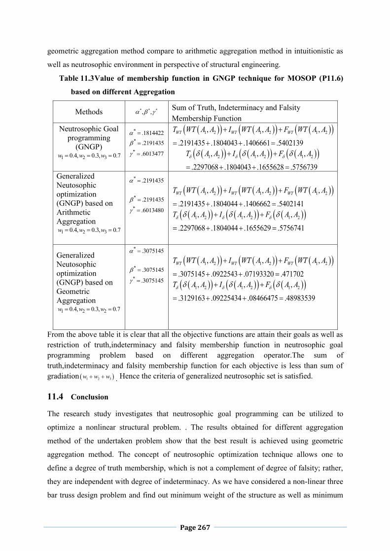
Page 267

geometric aggregation method compare to arithmetic aggregation method in intuitionistic as

well as neutrosophic environment in perspective of structural engineering.

Table 11.3 Value of membership function in GNGP technique for MOSOP (P11.6)

based on different Aggregation

Methods * * *, , Sum of Truth, Indeterminacy and Falsity Membership Function

Neutrosophic Goal programming

(GNGP) 1 2 30.4, 0.3, 0.7w w w

* .1814422

* .2191435

* .6013477

1 2 1 2 1 2, , ,

.2191435 .1804043 .1406661 .5402139WT WT WTT WT A A I WT A A F WT A A

1 2 1 2 1 2, , ,

.2297068 .1804043 .1655628 .5756739

T A A I A A F A A

Generalized Neutosophic optimization (GNGP) based on Arithmetic Aggregation

1 2 30.4, 0.3, 0.7w w w

* .2191435

* .2191435

* .6013480

1 2 1 2 1 2, , ,


1 2 1 2 1 2, , ,

.2297068 .1804044 .1655629 .5756741

T A A I A A F A A

Generalized Neutosophic optimization (GNGP) based on Geometric Aggregation

1 2 20.4, 0.3, 0.7w w w

* .3075145

* .3075145

* .3075145

1 2 1 2 1 2, , ,


1 2 1 2 1 2, , ,

.3129163 .09225434 .08466475 .48983539

T A A I A A F A A

From the above table it is clear that all the objective functions are attain their goals as well as restriction of truth,indeterminacy and falsity membership function in neutrosophic goal programming problem based on different aggregation operator.The sum of truth,indeterminacy and falsity membership function for each objective is less than sum of gradiation 1 2 3w w w . Hence the criteria of generalized neutrosophic set is satisfied.

11.4 Conclusion

The research study investigates that neutrosophic goal programming can be utilized to

optimize a nonlinear structural problem. . The results obtained for different aggregation

method of the undertaken problem show that the best result is achieved using geometric

aggregation method. The concept of neutrosophic optimization technique allows one to

define a degree of truth membership, which is not a complement of degree of falsity; rather,

they are independent with degree of indeterminacy. As we have considered a non-linear three

bar truss design problem and find out minimum weight of the structure as well as minimum

Page 268

deflection of loaded joint, the results of this study may lead to the development of effective

neutrosophic technique for solving other model of nonlinear programming problem in

different field.

Page 269

CHAPTER 12 Multi-objective Cylindrical Skin Plate Design Optimization based on

Neutrosophic Optimization Technique Structural optimization is an important notion in civil engineering. Traditionally structural optimization is a well known concept and in many situations it is treated as single objective form, where the objective is known the weight function. The extension of this is the optimization where one or more constraints are simultaneously satisfied next to the minimization of the weight function. This does not always hold good in real world problems where multiple and conflicting objectives frequently exist. In this consequence a methodology known as multi-objective structural optimization (MOSO) is introduced.In structural engineering design problems, the input data and parameters are often fuzzy/imprecise with nonlinear characteristics that necessitate the development of fuzzy optimum structural design method. Fuzzy set (FS) theory has long been introduced to handle inexact and imprecise data by Zadeh[133]. Later on Bellman and Zadeh [10] used the fuzzy set theory to the decision making problem. The fuzzy set theory also found application in structural design. Several researchers like Wang et al. [119] first applied α-cut method to structural designs where the non-linear problems were solved with various design levels α, and then a sequence of solutions were obtained by setting different level-cut value of α. Rao [89] applied the same α-cut method to design a four–bar mechanism for function generating problem. Structural optimization with fuzzy parameters was developed by Yeh et al. [132] Xu [13] used two-phase method for fuzzy optimization of structures. Shih et al. [95] used level-cut approach of the first and second kind for structural design optimization problems with fuzzy resources. Shih et al [96] developed an alternative α-level-cuts methods for optimum structural design with fuzzy resources. Dey et al. [32] used generalized fuzzy number in context of a structural design. Dey et al. [33] developed parameterized t-norm based fuzzy optimization method for optimum structural design. Also, Dey et.al[34] Optimized shape design of structural model with imprecise coefficient by parametric geometric programming. In such extension, Atanassov [1] introduced Intuitionistic fuzzy set (IFS) which is one of the generalizations of fuzzy set theory and is characterized by a membership function, a non membership function and a hesitancy function. In fuzzy sets the degree of acceptance is only considered but IFS is characterized by a membership function and a non-membership function so that the sum of both values is less than one. A transportation model was solved by Jana et al[57] using multi-objective intuitionistic fuzzy linear programming. Dey et al. [35] solved two bar truss non linear problem by using intuitionistic fuzzy optimization problem. Dey et al. [31] used intuitionistic fuzzy optimization technique for multi objective optimum structural design. Intuitionistic fuzzy sets consider both truth membership and falsity membership. Intuitionistic fuzzy sets can only handle incomplete information not the indeterminate information and inconsistent information.In neutrosophic sets indeterminacy is quantified explicitly and truth membership, indeterminacy membership and falsity membership which are independent. Neutrosophic theory was introduced by Smarandache [94] .The motivation of the present study is to give computational algorithm for solving multi-objective structural problem by single valued neutrosophic optimization approach. Neutrosophic optimization technique is very rare in application to structural optimization. We also aim to study the impact of truth membership,

Page 270

indeterminacy membership and falsity membership function in such optimization process. The results are compared numerically both in fuzzy optimization technique, intuitionistic fuzzy optimization technique and neutrosophic optimization technique. From our numerical result, it is clear that neutrosophic optimization technique provides better results than fuzzy optimization and intuitionistic fuzzy optimization.

12.1 Multi-objective Structural Model Formulation

In the design problem of the structure i.e. lightest thickness of the structure and minimum sag that satisfies all stress and deflection constraints in members of the structure. In vertical lift gate structural system ,the basic parameters (including allowable stress ,deflection etc) are known and the optimization’s target is that identify the optimal thickness and sag so that the structure is of the smallest total weight with minimum stress and deflection in a given load conditions . The multi-objective structural model can be expressed as

(P12.1) Minimize G (12.1) Minimize S (12.2)

subject to (12.3) (12.4)

min maxG G G (12.5) min maxS S S (12.6)

where G and S are the design variables for the structural design, is the deflection of the vertical lift gate of skin plate due to hydraulic load. is the stress constraint and , are allowable stress of the vertical lift gate of skin plate under various conditions. minG and minS ,

maxG and maxS are the lower and upper bounds of design variables respectively.

12.2 Solution of Multi-objective Structural Optimization Problem (MOSOP) by Neutrosophic Optimization Technique

To solve the MOSOP (P12.1), step 1 of 1.30 is used .After that according to step to pay off matrix is formulated.

1 1 1

2 2 2

G S

G G SS T S

According to step-2 the bound of weight objective , ;T TG GU L ,I I

G GU L and ,F FG GU L for truth,

indeterminacy and falsity membership function respectively. Then

;T TG GL G U ;F F

G GL G U I IG GL G U . Similarly the bound of deflection objective are , ;T T

S SU L

,F FS SU L and ,I I

S SU L are respectively for truth, indeterminacy and falsity membership function. Then ;T T

S SL S U ;F FS SL S U I I

S SL S U .Where ;F TG GU U ;F T

G G GL L ,I T I TG G G G GL L U L

and ;F TS SU U ;F T

S S SL L ;I TS SL L I T

S S SU L such that

0 T TG G GU L and 0 T T

S S SU L .

Page 271

According to neutrosophic optimization technique considering truth, indeterminacy and falsity membership function for MOSOP (P12.1), crisp non-linear programming problem can be formulated as

(P12.2) Maximize

subject to

;GT ;ST ;GF ;GF

;GI ;SI ; ;

3; ; ;

, , 0,1 , min maxG G G min maxS S S

Solving the above crisp model (6) by an appropriate mathematical programming algorithm we get optimal solution and hence objective functions i.e structural weight and deflection of the loaded joint will attain Pareto optimal solution.

12.3 Numerical Illustration

A cylindrical skin plate of vertical lift gate (Guha A.L et al [49]) in Fig-12.1 has been considered. The weight of the skin plate is about 40% of the weight of the vertical lift gate, thus the minimum weight of the vertical lift gate can be achieved by using minimum thickness of a skin plate with same number of horizontal girders for the particular hydraulic load. It is proposed to replace stiffened flat skin plate by unstiffened cylindrical skin plate. The stress developed in skin plate and its distribution mainly depends on water head, skin plate thickness, and sag and position of Horizontal girders. Stress and deflection are expressed in terms of water head, skin plate thickness, and sag based on finite element analysis.

Fig.-12.1 Vertical lift gate with cylindrical shell type skin plate

The proposed expressions are furnished as stress 31 21, , nn nG S H K G S H

where, stress in Kg/cm2; H water Head in ‘m’ G Thickness in ‘mm’ S Sag in ‘mm’

1K constant of variation and 1;n 2n and 3n constants depend on the properties of material Similarly,deflection 5 64

2, , n nnG S H K G S H where, 2K constant of variation and

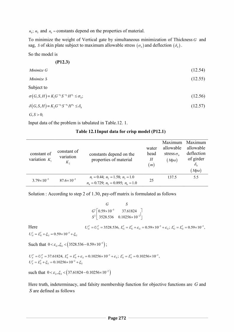
Page 272

4 ;n 5n and 6n constants depend on the properties of material.

To minimize the weight of Vertical gate by simultaneous minimization of Thickness G and sag, S of skin plate subject to maximum allowable stress 0 and deflection 0 .

So the model is (P12.3)

Minimize G (12.54)

Minimize S (12.55)

Subject to

31 21 0, , ;nn nG S H K G S H

(12.56)

5 642 0, , n nnG S H K G S H

(12.57)

, 0;G S

Input data of the problem is tabulated in Table.12. 1.

Table 12.1 Input data for crisp model (P12.1)

constant of variation 1K

constant of variation

2K constants depend on the properties of material

water head

H m

Maximum allowable stress 0 Mpa

Maximum allowable deflection of girder

0 Mpa

33.79 10 587.6 10 1 0.44;n 2 1.58;n 3 1.0n 4 0.729;n 5 0.895;n 6 1.0n 25

137.5 5.5

Solution : According to step 2 of 1.30, pay-off matrix is formulated as follows

1 5

2 2

0.59 10 37.618243528.536 0.10256 10

G S

GS

Here 3528.536,F TG GU U 50.59 10 ;F T

G G G GL L 50.59 10 ,I TG GL L

50.59 10I TG G G GU L

Such that 50 , 3528.536 0.59 10G G ;

37.61824,F TS SU U 20.10256 10 ;F T

S S S SL L 20.10256 10 ,I TS SL L

20.10256 10I TS S S SU L

such that 20 , 37.61824 0.10256 10S S

Here truth, indeterminacy, and falsity membership function for objective functions are G and S are defined as follows

Page 273

5

55

1 0.59 103528.536 0.59 10 3528.536

3528.536 0.59 100 3528.536

G

if GGT if G

if G

(12.58)

5

55

5

0 0.59 10

0.59 100.59 10 3528.536;

3528.536 0.59 101 3528.536

G

GG G

G

if G

GF if G

if G

(12.59)

5

55 5

5

1 0.59 10

0.59 100.59 10 0.59 10

0 0.59 10

GG G

G

G

if G

GI if G

if G

(12.60)

2

22

1 0.10256 1037.61824 0.10256 10 37.61824;

37.61824 0.10256 100 37.61824

S

if SST if S

if S

(12.61)

2

22

2

0 0.10256 10

0.10256 100.10256 10 37.61824;

37.61824 0.10256 101 37.61824

S

SS S

S

if S

SF if S

if S

(12.62)

2

22 2

2

1 0.10256 10

0.10256 100.10256 10 0.10256 10

0 0.10256 10

SS S

S

S

if S

SI if S

if S

(12.63)

Now using neutrosophic optimization technique with truth, indeterminacy and falsity membership functions we get

(P12.4) Maximize (12.64)

53528.536 0.59 10 3528.536;subject to G (12.65)

237.61824 0.10256 10 37.61824;S (12.66)

51 0.59 10 3528.536 ;GG (12.67)

21 0.10256 10 37.61824 ;SS (12.68)

Page 274

50.59 10 ;G GG (12.69)

20.10256 10 ;S SS (12.70)

3 0.44 1.583.79 10 25 137.5;G S (12.71)

5 0.729 0.89587.6 10 25 5.5;G S (12.72)

; (12.73)

; (12.74)

3; (12.75)

, , 0,1 (12.76)

Table 12.2 Comparison of Optimal solution of MOSOP (P12.1) based on different method

Methods G

mm

T

mm

Fuzzy multi-objective nonlinear programming (FMONLP) 52.88329 0.5648067

Intuitionistic fuzzy multi-objective nonlinear programming (IFMONLP)

1764.268, 2.57033G S 52.88329 0.5648065

Neutosophic optimization (NSO) 1764.268, 22.57033G G S S 44.28802 0.5676034

Here we get best solutions for the different tolerance ,G S for indeterminacy membership function of objective functions. From the Table 12.2, it shows that NSO technique gives better Pareto optimal result in the perspective of Structural Optimization.

12.4 Conclusion

The main objective of this work is to illustrate how much neutrosophic optimization technique reduce thickness and sag of nonlinear vertical lift gate in comparison of fuzzy and intuitionistic fuzzy optimization technique. The concept of neutrosophic optimization technique allows one to define a degree of truth membership, which is not a complement of degree of falsity; rather, they are independent with degree of indeterminacy. Here we have considered a non-linear skin plate of vertical lift gate problem .In this problem, we find out minimum thickness of the structure as well as minimum sag of cylindrical skin plate. The comparisons of results obtained for the undertaken problem clearly show the superiority of neutrosophic optimization over fuzzy optimization and intuitionistic fuzzy optimization. The results of this study may lead to the development of effective neutrosophic technique for solving other model of nonlinear programming problem in different field.

Page 275

APPENDIX-A

13.1 Crisp Set A set (crisp set) can be defined as the collection of well-defined distinct objects. For example

if the set of odd positive real numbers in between 0 20and be denoted by ,then in

tabular form it will be : 2 ,0 10x x n n and in set builder form it will be

2,4,6,8,10,12,14,16,18

13.2 Fuzzy Set A fuzzy set is an extension of the notion of crisp set such that their elements are

characterized by their grade of membership and non-membership.

Fuzzy Sets are Introduced by Zadeh [133] as means of modelling problems and

manipulating data that are not precise, in which the source of imprecisions is the absence of

sharply defined criteria of class membership. Fuzzy set is an extension of crisp set i.e a

classical set. Specially a fuzzy set on a classical set X is defined as follows

, :AA x x x X

(13.1)

where A x is termed as the grade of membership of x in A and the function

: 0,1A x X while assign the value 0 ,the member is not included in the given set and

while it assign 1 ,the member is fully included. The value strictly lies between 0 1and

characterized by the fuzzy numbers.

Fig.-13.1 Rough Sketch of Crisp Set and Membership Function of Fuzzy Set

In case of crisp set members are in the set with membership value 1 or out of the set the

membership value 0 .Thus crisp set fuzzy set. In other word crisp set is the special case of

Page 276

fuzzy set. For example if “tall women” is considered as a member in fuzzy set then it will be

considered as a member in crisp set when it ranged with 6 ft . Similarly a point near 10

in fuzzy while be ranged with 9.8,10.3 then it will be considered as an member in crisp set.

13.3 Height of a Fuzzy Set

The height of a fuzzy set A on X ,denoted by hgt A is the least upper bound of A x i.e

sup Ax X

hgt A x

(13.2)

13.4 Normal Fuzzy Set

A fuzzy set A is said to be normal if there exist at least one x X attaining the maximum

membership grade 1 (i.e 1hgt A ),otherwise it is subnormal .For optimized fuzzy set A

1Ax XMax x

(13.3)

13.5 Cut of Fuzzy Set

The cut of the fuzzy set A on X is crisp set that contains all the element of X that

have membership values in A greater than or equal to . i.e

: , , 0,1AA x x x X

(13.4)

13.6 Union of Two Fuzzy Sets

The union of two fuzzy sets A and B is a fuzzy set of X ,denoted by A B and is defined

by the membership function

BA B Ax x x for each x X (13.5)

so that , : max , ,BA B A B AA B x x x x x x X

(13.6)

or max , /BAx X

A B x x X

(13.7)

for any continuous fuzzy set ,A B .

13.7 Intersection of Two Fuzzy Sets

The intersection of two fuzzy sets A and B is a fuzzy set of X ,denoted by A B and is

defined by the membership function

BA B Ax x x for each x X (13.8)

so that

Page 277

, : min , ,BA B A B AA B x x x x x x X

(13.9)

min , /BAx X

A B x x X

(13.10)

for any continuous fuzzy set ,A B . 13.8 Convex Fuzzy Set

A fuzzy set A of universe of X is convex if and only if for all 1 2,x x in X

1 2 1 21 min ,A A Ax x x x when 0 1 (13.11)

13.9 Interval Number Interval analysis is a new and growing branch of applied mathematics. It provides necessary

calculus called interval arithmetic for interval numbers. An interval number can be thought as

an extension of the concept of a real number and also as a subset of real numbers. An interval

number A is defined by an ordered pair of real numbers as follows

, : ,L R L RA a a x a x a x R (13.12)

where La and Ra the left and right bounds of interval A respectively The interval A is also

defined by centre ca and half width wa as follows

, : ,c w c w c wA a a x a a x a a x (13.14)

where 2R L

ca aa

is the centre and 2R L

wa aa

is the half width of A .

The addition of two interval numbers ,L RA a a and ,L RB b b is defined as

, , ,L R L R L L R RA B a a b b a b a b (13.15)

,c w c w c c w wor A B a a b b a b a b (13.16)

Similarly the multiplication of an interval number by a scalar can be defined by

, 0

, 0L R

R R

kA ka ka if k

ka ka if k

(13.17)

or , ,c w c wkA k a a ka k a

(13.18)

13.10 Fuzzy Number A fuzzy number is a special case of a fuzzy set. Different definitions and properties of fuzzy

Page 278

numbers are encountered in the literature but they all agree on that fuzzy numbers represents

the conception of a set of „real numbers choose to a‟ ,where „a‟ is the number of fuzzy field.A

fuzzy number is a fuzzy set in the universe of discourse X i.e both convex and normal.

A Fuzzy number A is a fuzzy set defined on real line whose membership function A x

has the following characteristic with 1 2 3 4a a a a

1 2

2 3

3 4

1

0

L

AR

x for a x afor a x a

xx for a x a

for otherwise

(13.19)

where 1 2: , 0,1L x a a is continuous and strictly increasing; 3 4: , 0,1R a a is

continuous and strictly decreasing. The general shape of fuzzy number following the above

definition is shown below.

Fig.-13.2 Fuzzy Number

Fig.-13.2 Triangular Fuzzy number(TFN)

Let F be a set of all triangular fuzzy number in real line . A triangular fuzzy number

A F is fuzzy number with membership function : 0,1A parameterized by a

triplet 1 2 3, ,TFN

a a a and defined by

11 2

2 1

2

32 3

3 2

1

0

A

x a for a x aa a

for x ax

a x for a x aa a

otherwise

(13.20)

where 1a and 3a denote the lower and upper limits of support of a fuzzy number A

Page 279

Fig.-13.3 Triangular Fuzzy Number

2.10.1 Trapezoidal Fuzzy Number(TrFN)

Let F be a set of all trapezoidal fuzzy number in real line . A trapezoidal fuzzy

number A F is fuzzy number with membership function : 0,1A parameterized

by a quadruple 1 2 3 4, , ,TrFN

a a a a and defined by

11 2

2 1

2 3

43 4

4 3

1

0

A

x a for a x aa a

for a x ax

a x for a x aa a

otherwise

(13.21)

where 1a and 4a denote the lower and upper limits of support of a fuzzy number A

Fig.-13.4 Trapezoidal Fuzzy Number

13.11 Cut of Fuzzy Number

The level of a fuzzy number A is defined as a crisp set

: , , 0,1AA x x x X

(13.22)

. A is nonempty bounded closed interval contained in X and it can be denoted by

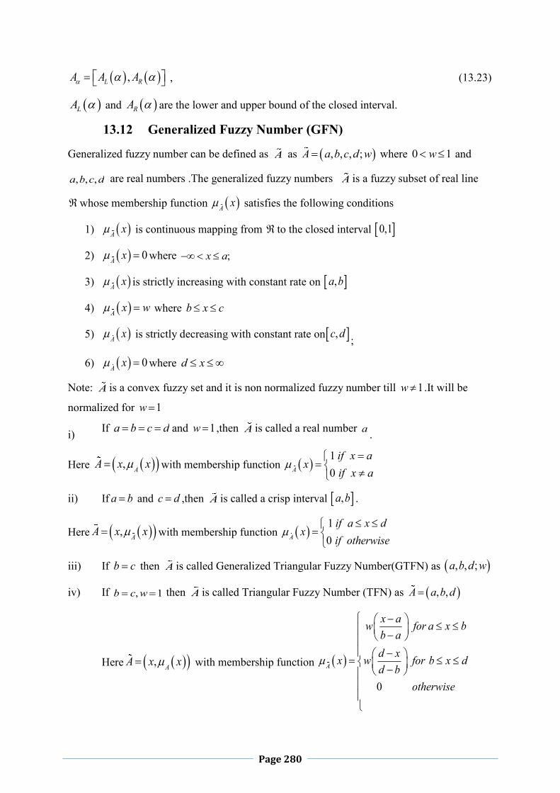
Page 280

,L RA A A , (13.23)

LA and RA are the lower and upper bound of the closed interval.

13.12 Generalized Fuzzy Number (GFN)

Generalized fuzzy number can be defined as A as , , , ;A a b c d w where 0 1w and

, , ,a b c d are real numbers .The generalized fuzzy numbers A is a fuzzy subset of real line

whose membership function A x satisfies the following conditions

1) A x is continuous mapping from to the closed interval 0,1

2) 0A x where ;x a

3) A x is strictly increasing with constant rate on ,a b

4) A x w where b x c

5) A x is strictly decreasing with constant rate on ,c d ;

6) 0A x where d x

Note: A is a convex fuzzy set and it is non normalized fuzzy number till 1w .It will be

normalized for 1w

i) If a b c d and 1w ,then A is called a real number a .

Here , AA x x with membership function 10A

if x ax

if x a

ii) If a b and c d ,then A is called a crisp interval ,a b .

Here , AA x x with membership function 10A

if a x dx

if otherwise

iii) If b c then A is called Generalized Triangular Fuzzy Number(GTFN) as , , ;a b d w

iv) If , 1b c w then A is called Triangular Fuzzy Number (TFN) as , ,A a b d

Here , AA x x with membership function

0

A

x aw for a x bb ad xx w for b x dd b

otherwise

Page 281

v) If b c then A is called Generalized Trapezoidal Fuzzy Number (GTrFN) and

denoted by , , , ;A a b c d w

vi) If , 1b c w then A is called Trapezoidal Fuzzy Number(TrFN) as , , ,A a b c d

Here , AA x x with membership function

0

A

x aw for a x bb aw for b x c

xd xw for c x dd c

otherwise

(13.24)

Traditional fuzzy arithmetic operations can deal with only normalized fuzzy numbers and

the type of membership function of fuzzy number are not changeable after arithmetic

operations. Thus Chen [31] proposed the function principle by which these fuzzy arithmetic

operations on fuzzy numbers does not only change the type of membership function after

arithmetic operation ,but they can also reduce the troublesomeness and tediousness of

arithmetical operations. Thus in this chapter ,we have introduced Chen‟s[31] fuzzy number

arithmetical operators to deal with the fuzzy number arithmetical operation of generalized

fuzzy numbers.The difference between the arithmetic operations on generalized fuzzy

numbers and the traditional fuzzy numbers is that the later can deal with only normalized

fuzzy number.

13.13 Nearest Interval Approximation of Fuzzy Number Here we want to approximate an fuzzy number 1 2 3, , ;A a a a w by a crisp model.

Let A and B be two fuzzy number with cuts ,L UA A and ,L UB B

respectively. Then the distance between them can be measured according to Euclidean matric

as 1 1

2 22

0 0E L L U Ud A B d A B d

(13.25)

Now we find a closed interval ,Ed L UC A C C which is nearest to A with respect to the

matric Ed .Again it is obvious that each real interval can also be considered as an fuzzy

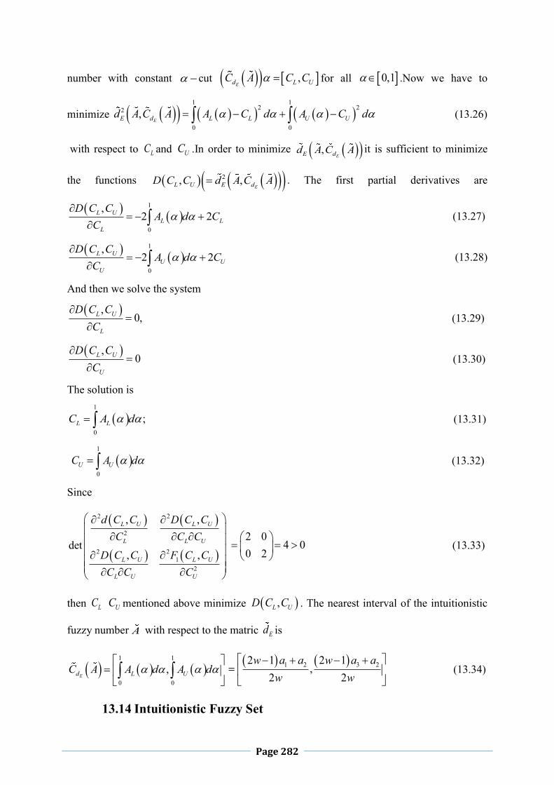
Page 282

number with constant cut ,Ed L UC A C C for all 0,1 .Now we have to

minimize 1 1

2 22

0 0

,EE d L L U Ud A C A A C d A C d

(13.26)

with respect to LC and UC .In order to minimize ,EE dd A C A it is sufficient to minimize

the functions 2, ,EL U E dD C C d A C A . The first partial derivatives are

1

0

,2 2L U

L LL

D C CA d C

C

(13.27)

1

0

,2 2L U

U UU

D C CA d C

C

(13.28)

And then we solve the system

,0,L U

L

D C CC

(13.29)

,0L U

U

D C CC

(13.30)

The solution is

1

0

;L LC A d

(13.31)

1

0U UC A d (13.32)

Since

2 2

2

2 21

2

, ,

det, ,

L U L U

L L U

L U L U

L U U

d C C D C CC C C

D C C F C CC C C

2 0

4 00 2

(13.33)

then LC UC mentioned above minimize ,L UD C C . The nearest interval of the intuitionistic

fuzzy number A with respect to the matric Ed is

1 1

0 0

,Ed L UC A A d A d

1 2 3 22 1 2 1,

2 2w a a w a a

w w

(13.34)

13.14 Intuitionistic Fuzzy Set

Page 283

Fuzzy set theory was first introduced by L.A.Zadeh [134] in 1965.Let X be the universe of

discourse defined by 1 2, ,..., nX x x x .The grade of membership of an element ix X in a

fuzzy set is represented by real value in 0,1 .It does indicate the evidence of ix X but does

not indicate the evidence against ix X .Attanassov [1] presented the concept of IFS.An IFS

iA in X is characterized by a membership function iAx and a nonmembership function

iAx .Here iA

x and iAx are associated with each point in X ,a real number in 0,1

with the values of iAx and iA

x at X representing the grade of membership and non-

membership of x in iA .When iA is an ordinary (crisp) set its membership function (non-

membership functions) can only take two values zero and one.An IFS becomes a fuzzy set

A when 0iAx but 0,1i

iA

x x A .Let a set X be fixed .An intuitionistic fuzzy

set iA in X is and object having the form

, , :i ii

A AA x x x x X

where : 0,1iAx X and : 0,1iA

x X define the degree of membership and

degree of nonmembership respectively of the element x X to the set iA ,which is a subset

of X ,for every element of x X , 0 1.i iA Ax x

(13.35)

13.15 , Level Or , Cuts

A set of , cut, generated by an IFS iA where , 0,1 are fixed number such that

1 is defined as

,

, , /, , , 0,1

i i

i i

i A A

A A

x x x x XA

x x

(13.36)

.We define , level or , cut ,denoted by ,iA

,as the crisp set of elements x

which belong to iA at least to the degree and which belong to iA at most to the degree .

13.16 Convex Intuitionistic Fuzzy Set An intuitionistic fuzzy set

, , :i ii

A AA x x x x X

(13.37)

is convex intuitionistic fuzzy set if

1 2 1 21 max ,i i iA A Ax x x x

(13.38)

Page 284

and 1 2 1 21 min ,i i iA A Ax x x x 1 2,x x X and 0 1 . (13.39)

13.17 Union Of Two Intuitionistic Fuzzy Sets

Let , , :i ii

A AA x x x x X and , , :i i

iB B

B x x x x X be two

intuitionistic fuzzy sets, then union of two intuitionistic fuzzy set will be defined by

,max , ,min , :i i i ii i

A B A BA B x x x x x x X

(13.40)

13.18 Intersection of Two Intuitionistic Fuzzy Sets

Let , , :i ii

A AA x x x x X and , , :i i

iB B

B x x x x X be two

intuitionistic fuzzy sets, then intersection of two intuitionistic fuzzy sets will be defined by

,min , ,max , :i i i ii i

A B A BA B x x x x x x X

(13.41)

13.19 Generalized Intuitionistic Fuzzy Number(GIFN)

A generalised intuitionistic fuzzy number iA can be defined with the following properties

i)It is an intuitionistic fuzzy subset of real line.

ii)It is normal i.e there exists 0x R such that 0iAx w R and 0iA

x R for

1;w

iii)It is a convex set for membership function iAx i.e

1 2 1 21 min ,i i iA A Ax x x x for all 1 2, , 0,x x R w .

iv) It is a concave set for non membership function iAx i.e

1 2 1 21 max ,i i iA A Ax x x x for all 1 2, , ,1x x R .

v) iA is continuous mapping from R to the closed interval 0, w and iA

is continuous

mapping from R to the closed interval ,1 and for 0x R the relation 1i iA A holds

13.20 Generalized Triangular Intuitionistic Fuzzy Number(GTIFN)

A generalized triangular intuitionistic fuzzy number 1 2 3 1 2 3, , ; , , ;ia aA a a a w a a a is a

intuitionistic fuzzy number in and can be defined with the following membership function

and non-membership function as follows

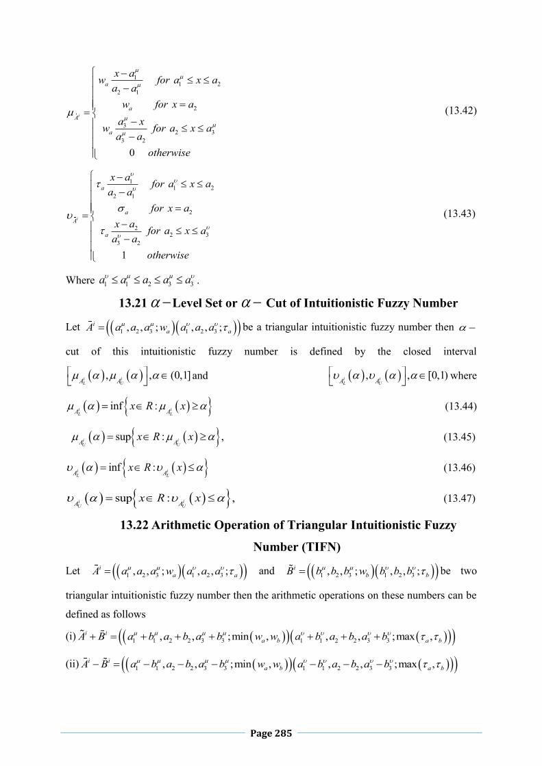
Page 285

11 2

2 1

2

32 3

3 2

0

i

a

aA

a

x aw for a x aa a

w for x aa xw for a x aa a

otherwise

(13.42)

11 2

2 1

2

22 3

3 2

1

i

a

aA

a

x a for a x aa a

for x ax a for a x a

a aotherwise

(13.43)

Where 1 1 2 3 3a a a a a .

13.21 Level Set or Cut of Intuitionistic Fuzzy Number

Let 1 2 3 1 2 3, , ; , , ;ia aA a a a w a a a be a triangular intuitionistic fuzzy number then

cut of this intuitionistic fuzzy number is defined by the closed interval

, , (0,1]i iL UA A

and , , [0,1)i iL UA A

where

inf :i iL LA A

x R x

(13.44)

sup : ,i i

U UA Ax R x

(13.45)

inf :i iL LA A

x R x

(13.46)

sup : ,i iU UA A

x R x

(13.47)

13.22 Arithmetic Operation of Triangular Intuitionistic Fuzzy

Number (TIFN)

Let 1 2 3 1 2 3, , ; , , ;ia aA a a a w a a a and 1 2 3 1 2 3, , ; , , ;i

b bB b b b w b b b be two

triangular intuitionistic fuzzy number then the arithmetic operations on these numbers can be

defined as follows

(i) 1 1 2 2 3 3 1 1 2 2 3 3, , ;min , , , ;max ,i ia b a bA B a b a b a b w w a b a b a b

(ii) 1 1 2 2 3 3 1 1 2 2 3 3, , ;min , , , ;max ,i ia b a bA B a b a b a b w w a b a b a b

Page 286

(iii)

1 2 3 1 2 3

3 2 1 3 2 1

, , ; , , ; 0

, , ; , , ; 0

a ai

a a

ka ka ka w ka ka ka for kkA

ka ka ka w ka ka ka for k

(iv)

1 1 2 2 3 3 1 1 2 2 3 3

1 3 2 2 3 1 1 3 2 2 3 1

3 3 2 2 1 1 3 3 2 2 1 1

, , ;min , , , ;max , 0, 0

. , , ;min , , , ;max , 0, 0

, , ;min , , , ;max ,

i ia b a b

i i i ia b a b

a b a b

a b a b a b w w a b a b a b for A B

A B a b a b a b w w a b a b a b for A B

a b a b a b w w a b a b a b fo

0, 0i ir A B

(v)

1 3 2 2 3 1 1 3 2 2 3 1

3 3 2 2 1 1 3 3 2 2 1 1

3 1 2 2 1 3 3 1 2 2

/ , / , / ;min , / , / , / ;max , 0, 0

/ / , / , / ;min , / , / , / ;max , 0, 0

/ , / , / ;min , / , / ,

i ia b a b

i i i ia b a b

a b

a b a b a b w w a b a b a b for A B

A B a b a b a b w w a b a b a b for A B

a b a b a b w w a b a b

1 3/ ;max , 0, 0i ia ba b for A B

13.23 Nearest Interval Approximation for Intuitionistic Fuzzy

Number Here we want to approximate an intuitionistic fuzzy number

1 2 3 1 2 3, , ; , , ;ia aA a a a w a a a by a crisp model.

Let iA and iB be two intuitionistic fuzzy number.Then the distance between them can be

measured according to Euclidean matric as

1 1 222

0 0

1 12 2L L U UE A B A Bd d d

1 1 22

0 0

1 12 2L L U UA B A Bd d (13.48)

Now we find a closed interval ,E

id L UC A C C which is nearest to iA with respect to the

matric Ed .Again it is obvious that each real interval can also be considered as an intuitionistic

fuzzy number with constant cut ,L UC C for all 0,1 .Now we have to minimize

,E

i iE dd A C A with respect to LC and UC ,that is to minimize

1 1 22

10 0

,L UL U A L A UF C C C d C d

1 1 22

0 0L UA L A UC d C d (13.49)

With respect to LC and UC . We define partial derivatives

Page 287

11

0

,2 4

L L

L UA A L

L

F C Cd C

C

(13.50)

11

0

,2 4

U U

L UA A U

U

F C Cd C

C

(13.51)

and then we solve the system

1 ,0,L U

L

F C CC

(13.52)

1 ,0L U

U

F C CC

(13.53)

The solution is

1

0

;2

L LA ALC d

(13.54)

1

0 2U UA A

UC d

(13.55)

Since

2 21 1

2

2 21 1

2

, ,4 0

det 4 00 4, ,

L U L U

L L U

L U L U

U L U

F C C F C CC C C

F C C F C CC C C

(13.56)

then LC UC mentioned above minimize 1 ,L UF C C . The nearest interval of the intuitionistic

fuzzy number iA with respect to the matric Ed is

1 1

0 0

,2 2

U UL L

E

A AA AidC A d d

(13.57)

2 3 3 2 3 21 2 2 1 2 1 ,2 4 4 2 4 4

a a a a a aa a a a a aw w

13.24 Parametric Interval Valued Function

If ,m n be an interval with , 0m n we can express an interval number by a function. The

parametric interval-valued function for the interval ,m n can be taken as

1 s sg s m n for 0,1s (13.58)

Page 288

which is strictly monotone continuous function and its inverse exists .Let be the inverse of

g s then log loglog log

msn m

. (13.59)

13.25 Ranking of Triangular Intuitionistic Fuzzy Number

A triangular intuitionistic fuzzy number 1 2 3 1 2 3, , ; , , ;ia aA a a a w a a a is completely

defined by

11 2

2 1a

x aL x w for a x aa a

(13.60)

and

32 3

3 2

;aa xR x w for a x aa a

(13.61)

21 2

2 1a

a xL x for a x aa a

(13.62)

and

22 3

3 2a

x aR x for a x aa a

. (13.63)

The inverse functions can be analytically express as

11 2 1 ;

a

hL h a a aw

(13.64)

13 3 2 ;

a

hR h a a aw

(13.65)

12 2 1 ;

a

hL h a a a

(13.66)

12 3 2 ;

a

hR h a a a

(13.67)

Now left integral value of membership and non-membership functions of iA are

1

1 21

0

2 12

aiL

a

w a aI A L h

w

(13.68)

and

1

1 21

0

2 12

aiL

a

a aI A L h

(13.69)

respectively

Page 289

and right integral value of membership and non-membership functions are

13 21

0

2 12

aiR

a

w a aI A L h

w

(13.40)

and

1

3 21

0

2 12

aiR

a

a aI A L h

(13.41)

respectively.

The total integral value of the membership functions is

2 3 13 2 1 2 2 1 12 1 2 1

12 2 2

aa aiT

a a a

a w a aw a a w a aI A

w w w

(13.42)

The total integral value of the non membership functions is

2 3 13 2 1 2 2 1 12 1 2 1

12 2 2

aa aiT

a a a

a a aa a a aI A

(13.43)

Now if 1 2 3 1 2 3, , ; , , ;ia aA a a a w a a a and 1 2 3 1 2 3, , ; , , ;i

b bB b b b w b b b be two

triangular intuitionistic fuzzy number then the following relations hold good

i) If i iT TI A I B and i i

T TI A I B for , 0,1 then i iA B

ii) If i iT TI A I B and i i


iii) If i iT TI A I B and i i


Page 290

APPENDIX-B

14.1 Geometric Programming(GP) Method

A Geometric Programming (GP) is a type of mathematical optimization problem

characterized by objective and constraint functions that have a special form. GP is a

methodology for solving algebraic non-linear optimization problems. Also linear

programming is a subset of a GP .The theory of GP was initially developed about three

decades ago and culminated in the publication of the seminal text in this area by Duffin,

Peterson, and Zener [134]

The general constrained Primal GP problem can be stated as follows

(P14.1) 0

00 0

1 1

( ) tj

T na

t jt j

Minimize f x c x

(14.1)

subject to

1 1

( ) ; 1,2,3,...,m

itj

T na

i it j it j

f x c x b i m

(14.2)

0, 1,2,..., .jx j n (14.3)

Here 0 0tc and 0tja be any real number. The objective function contains 0T terms and

inequality constraints contain iT terms. Here the coefficient of each term is positive. So it is a

constrained posynomial GP problem. Let 0 1 ......... iT T T T be the total number of

terms in the primal programme. The degree of difficulty (DD) is defined as DD = Total no. of

terms – (Total no. of variables -1) = ( 1)T n .The dual problem (with the objective function

( )d w ,where ( ), 0,1,2......, ; 1,2,.....it iw w w i m t T is the decision vector) of the GP

problem (P14.1) for the general posynomial case is as follows

(P14.2) 0

00

1 1 10

( )itt

iwwT Tm

it itt

t i tt i it

c wcMaximize d ww b w

(14.4)

subject to

0

01

1T

tt

w

, (Normality condition) (14.5)

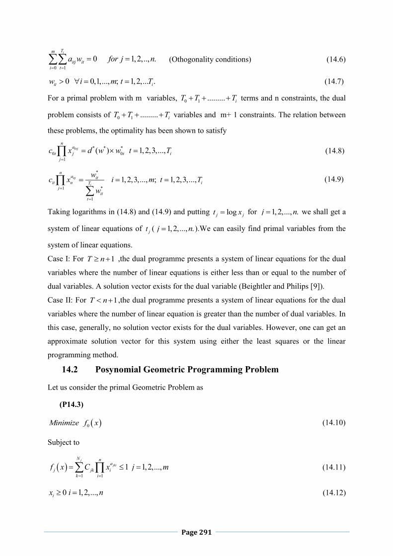
Page 291

0 10 1,2,.., .

iTm

itj iti t

a w for j n

(Othogonality conditions) (14.6)

0 0,1,..., ; 1,2,... .it iw i m t T (14.7)

For a primal problem with m variables, 0 1 ......... iT T T terms and n constraints, the dual

problem consists of 0 1 ......... iT T T variables and m+ 1 constraints. The relation between

these problems, the optimality has been shown to satisfy

0 * * *0 0

1

( ) 1,2,3,...,tjn

at j t i

j

c x d w w t T

(14.8)

*

*1

1

1,2,3,..., ; 1,2,3,...,itj

i

na it

it n iTj

itt

wc x i m t Tw

(14.9)

Taking logarithms in (14.8) and (14.9) and putting logj jt x for 1,2,..., .j n we shall get a

system of linear equations of jt ( 1,2,..., .j n ).We can easily find primal variables from the

system of linear equations.

Case I: For 1T n ,the dual programme presents a system of linear equations for the dual

variables where the number of linear equations is either less than or equal to the number of

dual variables. A solution vector exists for the dual variable (Beightler and Philips [9]).

Case II: For 1T n ,the dual programme presents a system of linear equations for the dual

variables where the number of linear equation is greater than the number of dual variables. In

this case, generally, no solution vector exists for the dual variables. However, one can get an

approximate solution vector for this system using either the least squares or the linear

programming method.

14.2 Posynomial Geometric Programming Problem

Let us consider the primal Geometric Problem as

(P14.3)

0Minimize f x (14.10)

Subject to

1 1

1j

jki

N na

j jk ik i

f x C x

1,2,...,j m (14.11)

0ix 1,2,...,i n (14.12)

Page 292


The dual problem of (P14.3) can be written as

0

0 1

jkj

wNmjk j

j k jk

C wMaximize d w

w

(14.13)

Subject to

01

1jN

kk

w

(Normality Condition) (14.14)

0 10

jNm

jki jkj k

a w

(Orthogonality Condition) (14.15)

01

0,jN

j jkk

w w

(14.16)

0,jkw

(14.17)

1,2,.., ;i n 1,2,.. ;jk N

00 1w . (14.18)

14.3 Signomial Geometric Programming Problem

Let us consider the primal Geometric Problem as

(P14.4)

0Minimize f x (14.19)

Subject to

1 1

jjki

N na

j jk jk i jk i

f x C x

1,2,...,j m (14.20)

0ix 1,2,...,i n (14.21)

Where 1, 0,1,2,.., ; 1,2,...,jk jj m k N and 1j jkia are all real numbers.

1 2, ,..., Tnx x x x

The dual problem of (P14.4) can be written as

Page 293

0

00

0 1

jk jkj

wNmjk j

j k jk

C wMaximize d w

w

(14.22)

Subject to

0 0 01

jN

k kk

w

(Normality Condition) (14.23)

0 10

jNm

jk jki jkj k

a w

(Orthogonality Condition) (14.24)

Where 1, 0,1,2,.., ; 1,2,...,jk jj m k N and 1j jkia are all real numbers.

1 2, ,..., Tnx x x x

01

0,jN

j j jk jkk

w w

(14.25)

0,jk

(14.26)

1,2,.., ;j m 1,2,.. ;jk N

00 1w . (14.27)

14.4 Fuzzy Geometric Programming(FGP)

A fuzzy geometric programming problem can be defined as

(P14.5) 0Minimize f x (14.28)

Subject to

j jf x b 1,2,...,j m (14.29)

0ix 1,2,...,i n

Here the symbol " "Minimize denotes a relaxed version of “Minimize”.Similarly the symbol “ ”denotes a fuzzy version of “ ”.These fuzy requrements may be quantified by taking

membership function , 0,1,2,....,j jf x j m from the decision maker for all functions

, 0,1,2,....,jf x j m by taking account of the rate of increased membership functions .It is

in general strictly monotone decreasing linear or non-linear function with respect to , 0,1,2,....,jf x j m .Here for simplicity linear membership functions are considered. The

linear membership function can be represented by

Page 294

0

'0 '

' 0

'

1

0

j j

j jj j j j j

j j

j j

if f x ff f x

f x if f f x ff f

if f x f

(14.30)

0,1,2,...,j m

The problem (P14.5) reduces to the FGP when 0f t and jf x are signomial and

posignomial functions.Based on fuzzy decision making of Bellmann and Zadeh(1972),we may write

i) * max minD j jx f x (Max-Min Operator)(14.31)

Subject to

0

'0 '

' 0

'

1

0

j j

j jj j j j j

j j

j j

if f x ff f x

f x if f f x ff f

if f x f

(14.32)

0,1,2,...,j m 1 2, ,..., Tnx x x x 0x

ii)

*

0max

m

D j j jj

x f x

(Max-Additive Operator) (14.33)

Subject to

0

'0 '

' 0

'

1

0

j j

j jj j j j j

j j

j j

if f x ff f x

f x if f f x ff f

if f x f

(14.34)

0,1,2,...,j m 1 2, ,..., Tnx x x x 0x

iii)

*

0

maxj

m

D j jj

x f x

(Max-Product Operator) (14.35)

Subject to

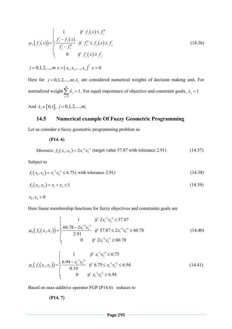
Page 295

0

'0 '

' 0

'

1

0

j j

j jj j j j j

j j

j j

if f x ff f x

f x if f f x ff f

if f x f

(14.36)

0,1,2,...,j m 1 2, ,..., Tnx x x x 0x

Here for 0,1,2,..., ; jj m are considered numerical weights of decision making unit. For

normalized weight0

1.m

jj

For equal importance of objective and constraint goals, 1j

And 0,1 ,j 0,1,2,..., ;j m

14.5 Numerical example Of Fuzzy Geometric Programming

Let us consider a fuzzy geometric programming problem as

(P14. 6)

2 30 1 2 1 2, 2Minimize f x x x x (target value 57.87 with tolerance 2.91) (14.37)

Subject to


2 1 2 1 2, 1f x x x x (14.39)

1 2, 0x x

Here linear membership functions for fuzzy objectives and constraints goals are

2 31 2

2 32 31 2

0 0 1 2 1 2

2 31 2

1 2 57.8760.78 2, 57.87 2 60.78

2.910 2 60.78


if x x

(14.40)

1 21 2

1 21 21 2

1 1 1 2 1 2

1 21 2

1 6.756.94, 6.75 6.94

0.190 6.94


if x x

(14.41)

Based on max-additive operator FGP (P14.6) reduces to

(P14. 7)

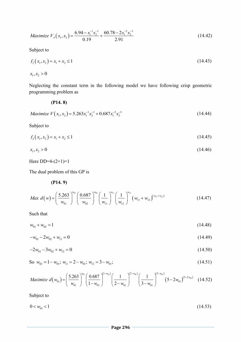
Page 296

1 1 2 3

1 2 1 21 2

6.94 60.78 2,0.19 2.91A

x x x xMaximize V x x

(14.42)

Subject to

2 1 2 1 2, 1f x x x x (14.43)

1 2, 0x x


(P14. 8)


(14.44)

Subject to

2 1 2 1 2, 1f x x x x (14.45)

1 2, 0x x (14.46)

Here DD=4-(2+1)=1


(P14. 9)

01 02 11 12

11 12

11 1201 02 11 12

5.263 0.687 1 1w w w w


(14.47)

Such that

01 02 1w w (14.48)

01 02 112 0w w w (14.49)

01 02 122 3 0w w w (14.50)

So 02 011 ;w w 11 012 ;w w 12 013 ;w w (14.51)

01 01 01 01

01

1 2 35 2

01 0101 01 01 01

5.263 0.687 1 1 5 21 2 3


w w w w

(14.52)

Subject to

010 1w (14.53)

Page 297

For optimality, 01

01

0d d w

dw (14.54)

2

01 01 01 01 015.263 1 2 3 0.687 5 2w w w w w (14.55)

*01 0.7035507,w *

02 0.2964493,w *11 1.296449,w *

12 2.296449,w (14.56)

*1 0.360836,x *

2 0.6391634,x (14.57)

* * *0 1 2, 58.82652,f x x * * *

1 1 2, 6.783684,f x x

14.6 Intuitionistic Fuzzy Geometric Programming

Consider an Intuitionistic Fuzzy Geometric Programming Problem as

(P14.10)

0

iMin f x (14.58)

Subject to

ij jf x b 1,2,..,j m (14.59)

0x

(14.60)

Here the symbol “ i ” denotes the intuitionistic fuzzy version of “ ”.Now for intuitionistic fuzzy geometric programming linear membership and non-membership can be represented as follows

0

'0 '

' 0

'

1

0

j j

j jj j j j j

j j

j j

if f x ff f x

f x if f f x ff f

if f x f

(14.61)

0,1,2,...,j m

' ''

' ''' '' '

''

'

1

0

j j j

j j jj j j j j j

j

j j

if f x f f

f x f ff x if f f f x f

fif f x f

(14.62)

0,1,2,...,j m

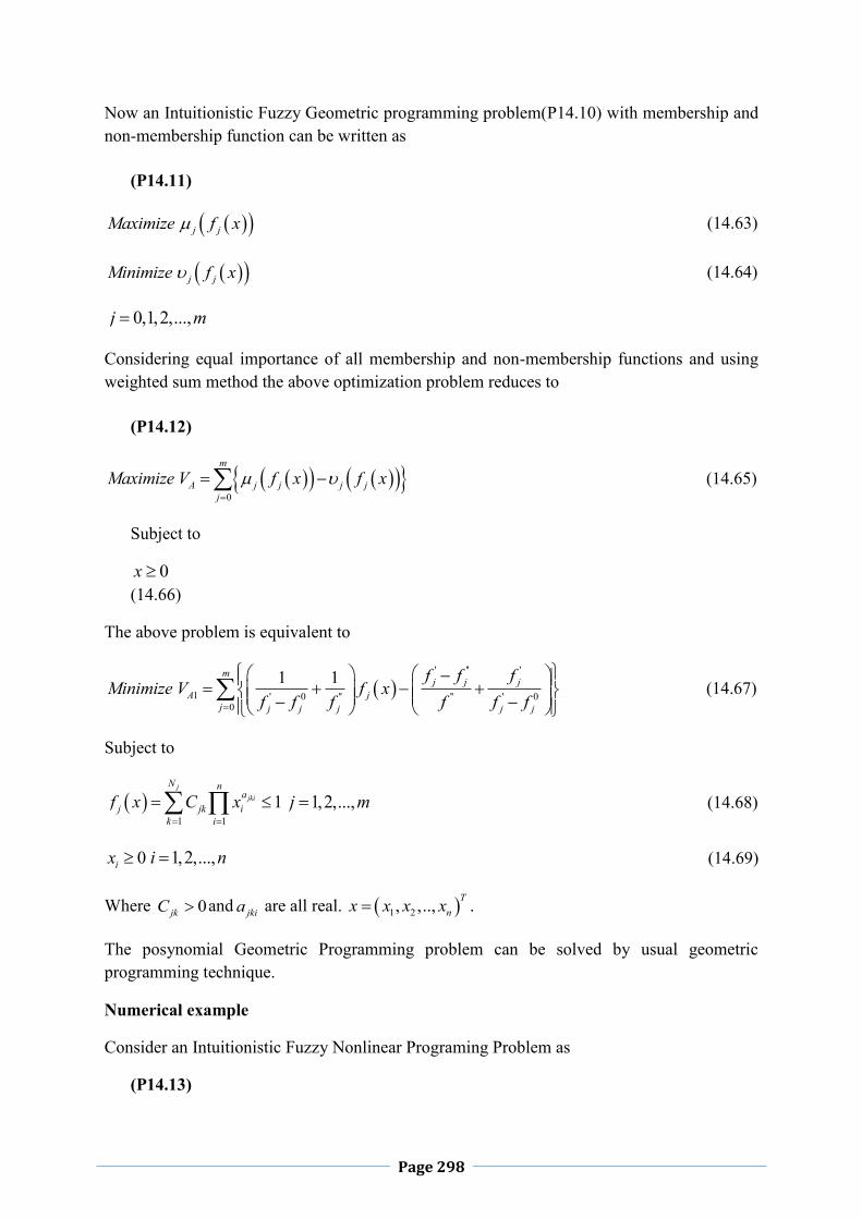
Page 298

Now an Intuitionistic Fuzzy Geometric programming problem(P14.10) with membership and non-membership function can be written as

(P14.11)


j jMinimize f x (14.64)

0,1,2,...,j m

Considering equal importance of all membership and non-membership functions and using weighted sum method the above optimization problem reduces to

(P14.12)

0

m

A j j j jj

Maximize V f x f x

(14.65)

Subject to

0x

(14.66)

The above problem is equivalent to

' '' '

1 ' 0 '' '' ' 00

1 1mj j j

A jj j j j j j

f f fMinimize V f x

f f f f f f

(14.67)

Subject to

1 1

1j

jki

N na

j jk ik i

f x C x

1,2,...,j m (14.68)

0ix 1,2,...,i n (14.69)


The posynomial Geometric Programming problem can be solved by usual geometric programming technique.

Numerical example

Consider an Intuitionistic Fuzzy Nonlinear Programing Problem as

(P14.13)

Page 299

2 30 1 2 1 2, 2

iMinimize f x x x x (target value 57.87 with tolerance 2.91) (14.70)

Subject to


2 1 2 1 2, 1f x x x x (14.72)

1 2, 0x x

Here linear membership and non-membership functions for fuzzy objectives and constraints goals are

2 31 2

2 32 31 2

0 0 1 2 1 2

2 31 2

1 2 57.8760.78 2, 57.87 2 60.78

2.910 2 60.78


if x x

(14.73)

1 21 2

1 21 21 2

1 1 1 2 1 2

1 21 2

1 6.756.94, 6.75 6.94

0.190 6.94


if x x

(14.74)

2 31 2

2 32 31 2

0 0 1 2 1 2

2 31 2

1 2 59.032 59.03, 59.03 2 60.78

1.750 2 60.78


if x x

(14.75)

1 21 2

1 21 21 2

1 1 1 2 1 2

1 21 2

1 6.836.83, 6.83 6.94

0.110 6.94


if x x

(14.76)

Based on max-additive operator FGP (14.13) reduces to

(P14.14)

1 1 2 31 2 1 2 1 2

1 1 1 1, 20.19 0.11 2.91 1.75AMaximize V x x x x x x

(14.77)

Subject to

2 1 2 1 2, 1f x x x x (14.78)

Page 300

1 2, 0x x


(P14.15)


(14.79)

Subject to

2 1 2 1 2, 1f x x x x (14.80)

1 2, 0x x (14.81)

Here DD=4-(2+1)=1


01 02 11 12

11 12

11 1201 02 11 12

14.354 1.828 1 1w w w w


(14.82)

Such that

01 02 1w w (14.83)

01 02 112 0w w w (14.84)

01 02 122 3 0w w w (14.85)

So 02 011 ;w w 11 012 ;w w 12 013 ;w w (14.86)

01 01 01 01

01

1 2 35 2

01 0101 01 01 01

14.354 1.828 1 1 5 21 2 3


w w w w

(14.87)

Subject to

010 1w (14.88)

For optimality, 01

01

0d d w

dw (14.89)

2

01 01 01 01 0114.354 1 2 3 1.828 5 2w w w w w (14.90)

*01 0.6454384,w *

02 0.3545616,w *11 1.3545616,w *

12 2.3545616,w (14.91)

Page 301

*1 0.365197,x *

2 0.63348027,x (14.92)

* * *0 1 2, 58.62182,f x x * * *

1 1 2, 6.795091,f x x

14.7 Fuzzy Decision Making

In this real world ,most of the decision making problems take place in a fuzzy environment.

The objective goal, constraints and consequences of possible actions are not known precisely.

Under this observation, Bellman et al. [10] introduced three basic concepts. They are fuzzy

objective goal, fuzzy constraint and fuzzy decision based on fuzzy goal and constraint. We

introduce the conceptual framework for decision making in a fuzzy environment .Let X be a

given set of possible alternatives which contains the solution of a decision making problem in

fuzzy environment. The problem based on fuzzy decision making may be considered as

follows

Optimize fuzzy goal G

Subject to constraint C

A Fuzzy goal , GG x x x X and a fuzzy constraint , CC x x x X is a

fuzzy set characterised by its membership function : 0,1G x X and : 0,1C x X

respectively. Both the fuzzy goal and fuzzy constraints are desired to be satisfied

simultaneously, So Bellman et al. [10] defined fuzzy decision through fuzzy goal and fuzzy

constraint.

14.8 Additive Fuzzy Decision

Fuzzy decision based on additive operator is a fuzzy set

,a DD x x x X

(14.93)

such that

a G CD x x for all x X . (14.94)

14.9 Intuitionistic Fuzzy Optimization(IFO) Technique to solve

Minimization Type Single Objective Non-linear Programming

(SONLP) Problem

Let us consider a SONLP problem as

(P14.16)

Page 302


1,2,......,j jg x b j m (14.96)

0x (14.97)

Usually constraints goals are considered as fixed quantity .But in real life problem,the


type constraints at least jb and it may possible to extend to 0j jb b .This fact seems to take the

constraint goal as a IFS and which will be more realistic descriptions than others. Then the

NLP becomes IFO problem with intuitionistic resources, which can be described as follows

(P14.17)


1,2,....,ij jg x b j m (14.99)

0x (14.100)

To solve the IFO (P14.16), following warner’s [118] and Angelov [3] we are presenting a

solution procedure for Single Objective Intuitionistic Fuzzy Optimization (SOIFO) problem

as follows

Step-1: Following Werner’s approach solve the single objective non-linear programming

problem without tolerance in constraints (i.e j jg x b ),with tolerance of acceptance in

constraints (i.e 0j j jg x b b ) by appropriate non-linear programming technique

Here they are

(P14.18)

Sub-problem-1


1,2,....,j jg x b j m (14.102)

0x (14.103) (P14.19)

Sub-problem-2


0 , 1,2,....,j j jg x b b j m (14.105)

Page 303

0x (14.106)

we may get optimal solutions * 1 * 1,x x f x f x and * 2 * 2,x x f x f x for sub-

problem 1 and 2 respectively.


functions. If

,f x f xU U be the upper bounds of membership and non-membership functions

for the objective respectively and

,f x f xL L be the lower bound of membership and non-

membership functions of objective respectively then

1 2max ,f xU f x f x (14.107)

1 2min , ,f xL f x f x

(14.108)

, 0f x f x f x f x f x f x f x f xU U L L where U L

(14.109)

Step-3: In this step we calculate linear membership for membership and non -membership

functions of objective as follows

1

0

f x

f xf x f x f x

f x f x

f x

if f x L

U f xf x if L f x U

U L

if f x U

(14.110)

0

1

f x

f xf x f x f x

f x f x

f x

if f x L

f x Lf x if L f x U

U L

if f x U

(14.111)

and exponential and hyperbolic membership for membership and non-membership functions

as follows

1

1 exp

0

f x

f xf x f x f x

f x f x

f x

if f x L

U f xf x if L f x U

U L

if f x U

(14.112)

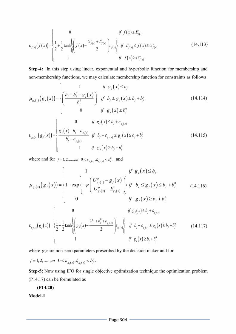
Page 304

0

1 1 tanh2 2 2

1

f x

f x f xf x f x f x f x

f x

if f x L

U Lf x f x if L f x U

if f x U

(14.113)

Step-4: In this step using linear, exponential and hyperbolic function for membership and

non-membership functions, we may calculate membership function for constraints as follows

00

0

0

1

0

j

j j

j j jj j j j jg x

j

j j

if g x b

b b g xg x if b g x b b

b

if g x b

(14.114)

00

0

0

1

j

j

j j

j

j j g x


j g x

j j j

if g x b

g x bg x if b g x b b

b

if g x b b

(14.115)

where and for

01,2,....., 0 ,j j jg x g xj m b . and

0

0

1

1 exp

0

j

j

j j

j j

jg xj j j j jg x

g x g x

j j j

if g x b

U g xg x if b g x b b

U L

if g x b b

(14.116)

00

0

0

21 1 tanh2 2 2

1

j

j

j j j

j j g x

j j g xj j j j j jg x g x g x

j j j

if g x b

b bg x g x if b g x b b

if g x b b

(14.117)


01,2,....., 0 ,

j j jg x g xj m b .

Step-5: Now using IFO for single objective optimization technique the optimization problem

(P14.17) can be formulated as

(P14.20)

Model-I

Page 305

Maximize (14.118)

such that

;f x x ;jg x

(14.119)

;f x x ;jg x

(14.120)

1; (14.121)

, 0,1 (14.122)

Now the above problem (P14.20)can be simplified to following crisp linear programming


(P14.21)

Maximize (14.123)

such that

. ;f x U L U

(14.124)

. ;f x f x f xf x U L L

(14.125)

1; ; , 0,1 ; (14.126)

0,j jg x b x

(14.127)

and for non linear membership function as

(P14.22)

Maximize (14.128)

such that

;

f x f x

f x

U Lf x U

(14.129)

;2

f x f x f x

f x

U Lf x

(14.130)

0

0;jj j j

bg x b b

(14.131)

Page 306

02

;2

jj j g xj

g x

b bg x

(14.132)

1; ; , 0,1 (14.133)

where ln 1 ; (14.134) 4; (14.135)

6 ;f x

f x f xU L

(14.136)

0

6 , 1,2,...,jg x

j j

for j mb

(14.137)

1tanh 2 1 . (14.138)

All these crisp nonlinear programming problems i.e (P14.21),(P14.22) can be solved by

appropriate mathematical algorithm.

14.10 Fuzzy Non-linear Programming (FNLP) Technique to Solve

Multi-Objective Non-Linear Programming (MONLP)problem

A Multi-Objective Non-Linear Programming (MONLP)problem may be considered in the

following form

(P14.23)

1 2, ,.....,T

pMinimize f x f x f x (14.139)

Subject to 1,2,...,j jg x b j m

(14.140)

0x (14.141)

Following Zimmermann [136] ,we have presented a solution algorithm to solve the MONLP

Problem by fuzzy optimization technique.

Step-1: Solve the MONLP (P14.23) as a single objective non-linear programming problem

p times by taking one of the objectives at a time and ignoring the others .These solutions are

known as ideal solutions. Let ix be the respective optimal solution for the thi different

objectives with same constraints and evaluate each objective values for all these thi optimal

solutions.

Page 307

Step-2: From the result of step -1 determine the corresponding values for every objective for

each derived solutions. With the values of all objectives at each ideal solutions ,pay-off

matrix can be formulated as follows

1 2

* 1 * 1 * 11 1 2

* 2 * 2 * 221 2

* * *1 2

....

......

......

...... ........ ...... .......

.....

p

p

p

pp p p

p

f x f x f x

f x f x f xxf x f x f xx

x f x f x f x

Here 1 2, ,.., px x x are the ideal solutions of the objectives 1 2, ,..., pf x f x f x

respectively.

Step-3: From the result of step-2,now we find lower bound (minimum) iL and upper bound

(maximum) iU by using the following rules

max ,i i pU f x (14.142)

mini i pL f x

(14.143)

where 1 i p .It is obvious * , 1ii iL f x i p .

Step-4: Using aspiration level of each objective, the MONLP (P14.23) may be written as

follows

(P14.24)

Find x so as to satisfy (14.144)

1,2,...,i if x L i p

(14.145)

1,2,...,j jg x b j m (14.146)

0x (14.147)

Here objective function of (P14.23) are consider as fuzzy constraints. This type of fuzzy

constraint can be quantified by eliciting a corresponding membership function

, 1,2,.....,i if x i p

Page 308

1

10

ACCi iACC ACCi i

ACCi i

f x Lw

U L wACC ACC

i i i i iw

ACCi i

if f x L

e ef x if L f x Ue

if f x U

(14.148)

Under the concept of mean operator , the feasible solution set is defined by intersection of

the fuzzy objective set .The feasible set is then characterized by its membership D x which

is 1 1 2 2min , ,...,D p px f x f x f x (14.149)

The decision solution can be obtained by solving the problem of

Dmaximize minimize x subject to the given constraints i.e

(P14.25)

0 i

Maximize Minimizex

x i

(14.150)

,j jsuch that g x b

(14.151)

0, 1,2,..., , 1,2,...,x j m i p (14.152)

Now if suppose iMinimize x be the overall satisfactory level of compromise, then we

obtain the following equivalent model

(P14.26)

Maximize (14.153)

, 1,2,...,isuch that x i p

(14.154)

, 1,2,....,j jg x b j m

(14.155)

0, 0,1x

(14.156)

Step-5: Solve (P14.26) to get optimal solution.

14.11 An Intuitionistic Fuzzy(IF) Approach for Solving Multi-

Objective Non-Linear Programming(MONLP) Problem with Non-

linear membership and Non-linear Non-membership Function

Following Zimmermann [140] and Angelov [3],we have presented a solution algorithm to

solve MONLP (P14.23) by Intuitionistic fuzzy optimization (IFO). Here Step 1 and Step 2

are same as shown in 14.10

Page 309

Step-3: From the result of step 2 now we find lower bound (minimum) ACCiL

and upper bound (maximum) ACCiU by using following rules

max ,ACC pi iU f x (14.157)

minACC pi iL f x where 1 i p . (14.158)

But in IFO the degree of non-membership (rejection) and the degree of membership

(acceptance) are considered so that the sum of both value is less than one. To define the non -

membership of NLP problem let Re jiU and Re j

iL be the upper bound and lower bound of

objective function if x where Re ReACC j j ACCi i i iL L U U .For objective function of

minimization problem ,the upper bound for non-membership function (rejection) is always

equals to that the upper bound of membership function (acceptance).One can take lower

bound for non-membership function as follows Re j Acci i iL L (14.159)

where 0 Acc Acci i iU L

based on the decision maker choice.

The initial IF model with aspiration level of objectives becomes , 1,2,....,iFind x i p

so as to satisfy

i Acci if x L with tolerance Acc Acc Acc

i i iP U L for the degree of acceptance for

1,2,....,i p (14.160)

Rei ji if x U with tolerance Acc Acc Acc

i i iP U L for degree of rejection for 1,2,....,i p

(14.161)

Define the membership (acceptance) and non-membership (rejection) functions of above

uncertain objectives as follows. For the , 1,2,....,thi i p objectives functions the linear

membership function i if x and linear non-membership i if x is defined as follows

Page 310

1

10

Acci i

Acc Acci i

Acci i

f x Lw

U L wAcc Acc

i i i i iw

Acci i

if f x L

e ef x if L f x Ue

if f U

(14.162)

Re

2ReRe Re

Re Re

Re

0

1

ji i

ji i j j

i i i i ij ji i

ji i

if f x L

f x Lf x if L f x U

U L

if f x U

(14.163)

Step-4: Now an IFO problem for above problem with membership and non-membership

functions can be written as

(P14.27)

i i

Maximizef x

i

(14.164)

i i

Minimizef x

i

(14.165)

1i i i isubject to f x f x

(14.166)

;i i i if x f x

(14.167)

0;i if x

(14.168)

0;jg x

(14.169)

0x (14.170)

1,2,...., ; 1,2,...,i p j m

Find an equivalent crisp model by using membership and non-membership functions of

objectives by IF decision making as follows

(P14.28)

1 2 1 2, ,.., , ,...,p pMax Min Min Max (14.171)

1i i i isubject to f x f x

(14.172)

;i i i if x f x

(14.173)

0;i if x

(14.174)

Page 311

0;jg x

0x (14.175)

1,2,.., ; 1,2,...,i p j m

If we consider

1 2, ,...., ;pMinimize

(14.176)

1 2, ,...., pMaximize

(14.177)

accordingly the Angelov [4], the above can be written as

(P14.29)

Maximize (14.178)

;i isubject to f x

(14.179)

0;jg x

(14.180)

0, 1x (14.181)

0,1 , 0,1 ; 1,2,...,i p

(14.182)

1,2,...,j m (14.183)

which on substitution of 1,2,....,i i i if x and f x for i p becomes

(P14.30)

( )Maximize (14.184)

subject to

ln 1 ;Acc Acc

w w Acci ii i

U Lf x e e Lw

(14.185)

Re Re Re ;j j ji i i if x U L L

(14.186)

0;jg x

(14.187)

1; (14.188)

0,1 , 0,1

(14.189)

1,2,.., ; 1,2,..,i p j m (14.190)

Step-5: Solve the above crisp model (P14.30) by using appropriate mathematical

programming algorithm to get optimal solution of objective function.

Step-6: Stop.

Page 312

14.12 Intuitionistic Fuzzy Non-linear Programming (IFNLP)

Optimization to solve Parametric Multi-Objective Non-linear

Programming Problem (PMONLP)

A multi-objective IFNLP problem with imprecise co-efficient can be formulated as

(P14.31)

0

0

0 0 01 1

kk tj

T na

k k t k t jt j

Minimize f x c x

for 0 1,2,....,k p (14.191)

Such that 1 1

iitj

T na

i it it j i it j

f x c x b

for 1,2,....,i m (14.192)

0jx 1,2,....,j n (14.193)

Here 0

,k t ,it i are the signum function used to indicate sign of term in the equation.

00,k tc 0itc .

0,k tja itja are real numbers for all 0, , , .i t k j

Here 0 0 0 0 0 0 0 0 0

1 2 3 1 2 3, , ; , , ; ;k t k t k t k t k t k t k t k t k tc c c c w c c c

(14.194)

1 2 3 1 2 3, , ; , , ; ;it it it it it it it it itc c c c w c c c

(14.195)

1 2 3 1 2 3, , ; , , ;i i i i i i i i ib b b b w b b b

(14.196)

Using total integral value of membership and non-membership functions, we transform above

multi-objective intuitionistic programming with imprecise parameter as

(P14.32)

0

0

0 0 01 11 1

ˆ ˆ;k

k tj

T na

k k t k t jt j

Minimize f x c x

for 0 1,2,...,k p (14.197)

0

0

0 0 02 21 1

ˆ ˆ;k

k tj

T na

k k t k t jt j

Minimize f x c x

for 0 1,2,...,k p (14.198)

Such that 1 1 11 1

ˆ ˆˆ;i

itj

T na

i it it j i it j

f x c x b

for 1,2,...,i m (14.199)

2 2 21 1

ˆ ˆˆ;i

itj

T na

i it it j i it j

f x c x b

for 1,2,....,i m (14.200)

0; , 0,1jx 1,2,....,j n (14.201)

Page 313

Here 0

,k t ,it i are the signum functions used to indicate sign of term in the equation.

01̂ 0,k tc 1̂ 0;itc 1̂ 0ib denote the total integral value of membership function i.e

0 0 0 0

0

0

2 3 1

1

2 1 1ˆ ,

2k t k t k t k t

k tk t

c w c cc

w

(14.202)

2 3 1

1

2 1 1ˆ

2it it it it

itit

c w c cc

w

(14.203)

and 2 3 1

1

2 1 1ˆ2

i i i ii

i

b w b bb

w

(14.204)

and 01̂ 0,k tc 1̂ 0;itc 1̂ 0ib denote the total integral value of non-membership function ie

0 0 0 0

0

0

2 3 1

2

2 1 1ˆ ,

2k t k t k t k t

k tk t

c c cc

(14.205)

2 3 1

2

2 1 1ˆ

2it it it it

itit

c c cc

(14.206)

and

2 3 1

2

2 1 1ˆ2

i i i ii

i

b b bb

(14.207)

A Parametric Multi-Objective Intuitionistic Fuzzy Non-Linear Programming

(PMOIFNLP)Problem can be formulated as

(P14.33)

1 2 1 2; , ; ,...., ; , ; , ; ,...., ;

T

p pMinimize f x f x f x f x f x f x

(14.208)

Subject to ; ; 1,2,...,j jg x b j m (14.209)

; ; 1,2,...,j jg x b j m (14.210)

0x , 0,1 (14.211)

Following Zimmermann [140]we have presented a solution algorithm to solve the

PMOIFNLP Problem by fuzzy optimization technique.

Step-1: Solve the PMOIFNLP (P14.33) as a SONLPP p times by taking one of the objectives

at a time and ignoring the others .These solutions are known as ideal solutions. Let ix be the

respective optimal solution for the thi different objectives with same constraints and evaluate

each objective values for all these thi optimal solutions.

Page 314

Step-2: From the result of step -1 determine the corresponding values for every objective for

each derived solutions. With the values of all objectives at each ideal solutions ,pay-off

matrix can be formulated as follows

1 1

* 1 * 1 * 1 * 11 1 1

* 2 * 2 * 2 * 221 1

2* 2 * 2 * 2 * 2

1 1

; ... ; ; ... ;

; ... ; ; ... ;

; ... ; ; ... ;

... ... ... ... ... ...

; ... ; ; ... ;

p p

p p

p p

pp p p p

p p

f x f x f x f x

f x f x f x f xxf x f x f x f xx

x f x f x f x f x

Here 1 2, ,......, px x x is the ideal solutions of the objectives

1 2 1 2; , ; ,...., ; , ; , ; ,...., ;p pf x f x f x f x f x f x respectively.

Step-3: From the result of step 2 now we find lower bound (minimum) ACCiL

and upper bound (maximum) ACCiU by using following rules

max ; , ; ,ACC p pi i iU f x f x (14.212)

min ; , ;ACC p pi i iL f x f x

(14.213)

where 1 i p .But in IFO The degree of non-membership (rejection) and the degree of

membership (acceptance) are considered so that the sum of both value is less than one. To

define the non -membership of NLP problem let Re jiU and Re j

iL be the upper bound and lower

bound of objective function , , ,i if x f x where Re ReACC j j ACCi i i iL L U U .For

objective function of minimization problem ,the upper bound for non-membership function

(rejection) is always equal to that the upper bound of membership function (acceptance).One

can take lower bound for non-membership function as follows Re j Acci i iL L (14.214)

where 0 Acc Acci i iU L based on the decision maker choice.

The initial IF model with aspiration level of objectives becomes

Find

, 1,2,..,ix i p (14.215)

so as to satisfy i Acci if x L with tolerance Acc Acc Acc

i i iP U L for the degree of acceptance

for 1,2,...,i p . (14.216)

Page 315

Re; i ji if x s U with tolerance Acc Acc Acc

i i iP U L for degree of rejection for 1,2,...,i p

(14.217)

Define the membership (acceptance) and non-membership (rejection) functions of above

uncertain objectives as follows. For the , 1,2,....,thi i p objective functions the linear

membership functions ;i if x and ;i if x and linear non-membership functions

;i if x and ;i if x are defined as follows

;

1 ;

; ;10 ;

Acci i

Acc Acci i

Acci i

f x LT

U L TAcc Acc

i i i i iT

Acci i

if f x L

e ef x if L f x Ue

if f x U

(14.218)

;

1 ;

; ;10 ;

Acci i

Acc Acci i

Acci i

f x LT

U L TAcc Acc

i i i i iT

Acci i

if f x L

e ef x if L f x Ue

if f x U

(14.219)

Re

2ReRe Re

Re Re

Re

0 ;

;; ;

1 ;

ji i

ji i j j

i i i i ij ji i

ji i

if f x L

f x Lf x if L f x U

U L

if f x U

(14.220)

Re

2ReRe Re

Re Re

Re

0 ;

;; ;

1 ;

ji i

ji i j j

i i i i ij ji i

ji i

if f x L

f x Lf x if L f x U

U L

if f x U

(14.221)

Step-4: Now using IF probabilistic operator above problem can be written as

(P14.34)

1

; ;p

i i i ii

Maximize f x f x

(14.222)

Page 316

1

1 ; 1 ;p

i i i ii

Maximize f x f x

(14.223)

subject to

0 ; 1;i if x

(14.224)

0 ; 1;i if x

(14.225)

0 ; ; 1;i i i if x f x (14.226)

0 ; 1;i if x

(14.227)

0 ; 1;i if x (14.228)

0 ; ; 1;i i i if x f x (14.229)

; ;j jg x b (14.230)

; ;j jg x b (14.231)

0x , 0,1 (14.232)

1,2,.., ; 1,2,...,i p j m (14.233)

Step-5: Solve the above crisp model (P14.34) by using appropriate mathematical

programming algorithm to get optimal solution of objective function.

Step-6: Stop.

14.13 Fuzzy and Intuitionistic Fuzzy Non-linear Programming

(IFNLP) Optimization to solve Parametric Single-Objective Non-

linear Programming (PSONLP) Problem

A multi-objective IFNLP with imprecise co-efficient can be formulated as

(P14.35)

1 1

tjnT

at t j

t j

Minimize f x c x

(14.234)

Such that 1 1

iitj

T na n

i it it j i it j

f x c x b

for 1,2,....,i m (14.235)

0jx 1,2,....,j n (14.236)

Here ,t ,it i are the signum functions used to indicate sign of term in the equation. 0,tc

0itc . ,tja itja are real numbers for all , , .i t j

Page 317

Here 1 2 3, , ; ;t t t t tc c c c w

(14.237)

1 2 3, , ; ;it it it it itc c c c w

(14.238)

1 2 3, , ;i i i i ib b b b w

(14.239)

for fuzzy number as coefficients and

1 2 3 1 2 3, , ; , , ; ;t t t t t t t t tc c c c w c c c

(14.240)

1 2 3 1 2 3, , ; , , ; ;it it it it it it it it itc c c c w c c c

(14.241)

1 2 3 1 2 3, , ; , , ;i i i i i i i i ib b b b w b b b (14.242)

for IF coefficient.

Using nearest interval approximation method for both fuzzy and IFN ,we transform all the

TIFN into interval number i.e , ,L Ut tc c , ,L U

it itc c and ,L Ui ib b

Now the MOIFNLP with imprecise parameter is of the following form

(P14.36)

0

1 1

ˆ ˆ tjnT

ak t t j

t j

Minimize f x c x

(14.243)

Such that 1 1

ˆ ˆˆi

itj

T na

i it it j i it j

f x c x b

for 1,2,....,i m (14.244)

0jx 1,2,....,j n (14.245)

Here ,t ,it i are the signum functions used to indicate sign of term in the equation. ˆ 0,tc

ˆ 0;itc ˆ 0ib denote the interval component i.e

ˆ , ,L Ut t tc c c

(14.246)

ˆ , ,L Uit it itc c c

(14.247)

and ˆ ,L Ui i ib b b

(14.248)

and

,tja itja are real numbers for all , , .i t j

Using parametric interval valued function the above problem transforms into

(P14.37)

1

1 1

; tjnT s s aL U

t t t jt j

Minimize f x s c c x

(14.249)

Page 318

such that 1 1

1 1

;i

itj

T ns s s saL U L Ui it it it j i i i

t j

f x s c c x b b

for 1,2,...,i m (14.250)

0jx 1,2,...,j n 0,1s

(14.251)

Here ,t ,it i are the signum functions used to indicate sign of term in the equation.

This is a parametric single objective non-linear programming problem and can be solved by

IFO technique.

Let us consider a Single-Objective Parametric Nonlinear Programming Problem(SOPNLPP)

as

(P14.38)

;Minimize f x s (14.252)

; 1,2,..,j jg x s b s j m

(14.253)

0; 0,1x s

(14.254)

Usually constraint goals are considered as fixed quantity .But in real life problem ,the


type constraints at least jb s and it may possible to extend to 0jb s so that the maximum

allowable tolerance is 1jb s with 0 1

j j jb s b s b s .This fact seems to take the constraint

goal as a IFS and which will be more realistic descriptions than others. Then the NLP

becomes IFO problem with IF resources, which can be described as follows

(P14.39)


; 1,2,....,ij jg x s b s j m (14.256)

0; 0,1x s (14.257)

To solve the IFO (P14.39) following Werner’s [118] and Angelov [3] we are presenting a

solution procedure for Single Objective Neutrosophic Optimization (SONSO) problem as

follows

Step-1: Following Warner’s approach solve the SONLP without tolerance in constraints (i.e

;j jg x s b s ),with tolerance of acceptance in constraints (i.e 0;j jg x s b s ) by

appropriate non-linear programming technique.

Here they are

(P14.40)

Page 319

Sub-problem-1


; 1,2,...,j jg x s b s j m

(14.259)

0; 0,1x s

(14.260)

(P14.41)

Sub-problem-2


0; , 1,2,....,j jg x s b s j m

(14.262)

0; 0,1x s

(14.263)

we may get optimal solutions * 1 * 1, ; ;x x f x s f x s and * 2 * 2, ; ;x x f x s f x s for sub-

problem 1 and 2 respectively.


functions. If ; ;,f x s f x sU U be the upper bounds membership and non-membership functions

for the objective respectively and ; ;,f x s f x sL L be the lower bounds of membership and non-

membership functions of objective respectively then

1 2; max ; , ; ,f x sU f x s f x s (14.264)

1 2; min ; , ; ,f x sL f x s f x s

(14.265)

; ; ; ; ; ; ; ;, 0f x s f x s f x s f x s f x s f x s f x s f x sU U L L where U L (14.266)

Step-3: In this step we calculate linear membership for membership and non-membership

functions of objective as follows

;

;; ; ;

; ;

;

1 ;

;; ;

0 ;

f x s

f x sf x s f x s f x s

f x s f x s

f x s

if f x s L

U f x sf x s if L f x s U

U L

if f x s U

(14.267)

Page 320

;

;; ; ;

; ;

;

0 ;

;; ;

1 ;

f x s

f x sf x s f x s f x s

f x s f x s

f x s

if f x s L

f x s Lf x s if L f x s U

U L

if f x s U

(14.268)

Step-4: In this step using linear function for membership and non-membership functions, we

may calculate membership and non-membership function for constraints as follows

00

; 1

0

1 ;

;; ;

0 ;

j

j j

j jj j j jg x s

j

j j

if g x s b s

b s g x sg x s if b s g x s b s

b s

if g x s b s

(14.269)

;

; 0; ;1

;

0

0 ;

;; ;

1 ;

j

j

j j

j

j j g x s

j j g x sj j j jg x s g x s

j g x s

j j

if g x s b s

g x s b sg x s if b s g x s b s

b s

if g x s b s

(14.270)

where and for 1;1,2,....., 0

j jg x sj m b s .

0; 0,1x s

(14.271)

Step-5: Now using Fuzzy and IFO for single objective optimization technique(Singh .et.al

[93]) the optimization problem (P14.39) can be formulated as

(P14.42)

Maximize (14.272)

Such that

; ; ;f x s x s ; ;jg x s

(14.273)

0,1 0; 0,1x s

(14.274)

and

(P14.43)

Maximize

(14.275) Such that

;f x x ; ;jg x s

(14.276)

Page 321

;f x x ; ;jg x s

(14.277)

1; (14.278)

, 0,1 0; 0,1x s

(14.279)

In fuzzy and IF environment respectively. Now the above problem (P14.42),(P14.43) can be

Solved by appropriate mathematical programming

Page 322

Bibliography [1] Atanassov, K. T. (1986). Intuitionistic fuzzy sets. Fuzzy sets and Systems, 20(1), 87-

96.

[2] Atanassov, K. T. (1989). More on intuitionistic fuzzy sets. Fuzzy sets and

systems, 33(1), 37-45.

[3] Angelov, P.P.( 1995). Intuitionistic fuzzy optimization. Notes on Intutionistic Fuzzy

Sets 1 (2), 123-129.

[4] Angelov, P. P. (1997). Optimization in an intuitionistic fuzzy environment. Fuzzy

sets and Systems, 86(3), 299-306.

[5] Aguirre,A.H.,Zavala,A.M.,Diharce,E.V.,Rionda ,S.B.:COPSO:Constrained

Optimization via PSO Algorithm.Centre for Research in

Mathematics(CIMAT).(2007).Technical report No.I-07-04/22-02-2007.

[6] Alsina, C., Trillas, E., & Valverde, L. (1983). On some logical connectives for fuzzy

sets theory. Journal of Mathematical Analysis and Applications, 93(1), 15-26.

[7] Ali,Nicholas., Behdinan, Kumaran and Fawaz,Zouheir.(2003). Applicability and

Viability of a GA based Finite Element Analysis Architecture for Structural Design

Optimization. Computers and Structures, 81,2259-2271.

[8] Abdel-Baset, M., Hezam, I. M., & Smarandache, F. (2016). Neutrosophic goal

programming. Neutrosophic Sets Syst, 11, 112-118.

[9] Beightler,C.S.&Phillips,D.T.(1976).Applied Geometric Programming. Wiley, New

York.

[10] Bellman, R. E., &Zadeh, L. A. (1970).Decision-making in a fuzzy

environment. Management science, 17(4), B-141.

[11] Bharti, S.K., & Singh , S. R. Solving Multi-objective Linear Programming

Problems using Intuitionistic Fuzzy Optimization Method :A Comparative

Study. International Journal of Modelling and applications, Vol.4,Issue.1, (2014).

,10-16.

[12] Beightler,C.S. ,Philips,D.T. & Wilde, D.J :Foundation of

optimization,Prentice hall,New Jersy ,1979.

[13] Changwen, X. (1989). Fuzzy optimization of structures by the two-phase

method. Computers & Structures, 31(4), 575-580.

Page 323

[14] Coello, C. A. C. (2000). Use of a self-adaptive penalty approach for

engineering optimization problems. Computers in Industry, 41(2), 113-127.

[15] Coello Coello,C.A.,Montes,E.M.(2002).Contraint-handling techniques in

genetic algorithms through dominance based tournament selection.Advanced

Engineering Informatics,16,193-203.

[16] Coello Coello, C. A., & Becerra, R. L. (2004). Efficient evolutionary

optimization through the use of a cultural algorithm. Engineering

Optimization, 36(2), 219-236.

[17] Congress, I. R. (2002). Guidelines for the design of plain jointed rigid

pavements for highways. IRC.

[18] Cao, B.Y. (1987). Solution and theory of question for a kind of fuzzy positive

geometric program. Proceeding of the second IFSA Congress, Tokyo, 1, 205-208.

[19] Charia,T., Roy.A.,(2008).Anew Measure using Intuitionistic Fuzzy Set Theory

and Its Application to Edge Detection. Applied Soft Computing ,8(2),917-927.

[20] Chen,S.H.(1985).Operations in Fuzzy Numbers with Functin

Principal,Tamkang Journal of Management Science,6(1),13-25.

[21] Chibani, L. (2012). Optimum design of structures: with special reference to

alternative loads using geometric programming (Vol. 50). Springer Science &

Business Media.

[22] Coello Coello,C.A.,Montes,E.M.(2002).Contraint-handling techniques in

genetic algorithms through dominance based tournament selection.Advanced

Engineering Informatics,16,193-203.

[23] Coello Coello, C. A., & Becerra, R. L. (2004). Efficient evolutionary

optimization through the use of a cultural algorithm. Engineering

Optimization, 36(2), 219-236.

[24] Charns, A., & Cooper, R. (1961). Management Models and Industrial

Application of Linear Programming.

[25] Cagnina, L. C., Esquivel, S. C., & Coello, C. A. C. (2008). Solving

engineering optimization problems with the simple constrained particle swarm

optimizer. Informatica, 32(3).

[26] Chvorinov, N. (1939). Control of the Solidification of Castings by

Calculation. Foundry Trade Journal, 70(8), 95-98.

[27] Creese, R. C. (1971). Optimal riser design by geometric programming. AFS

cast metals research journal, 7(2), 118-121.

Page 324

[28] Creese, R. C. (1971). Dimensioning of riser for long freezing range alloys by

geometric programming. AFS cast metals research journal, 7(4), 182-185.

[29] Cao,B.Y. (1993).Fuzzy geometric programming.Fuzzy Sets and Systems,

53,135-153,.

[30] Cao,B.Y. Fuzzy geometric programming.Kluwar Academic

Publishers,Netherland 2002.

[31] Dey,S.,Roy,T.K.(2015).Multi-Objective Structural using Fuzzy and

Intuitionistic Fuzzy Optimization Technique ,International Journal of Intelligent

Systems and Applications.5,57-65.

[32] Dey, S., & Roy, T. K. (2014). A Fuzzy programming Technique for Solving

Multi-objective Structural Problem. International Journal of Engineering and

Manufacturing, 4(5), 24.

[33] Dey,S.,Roy,T.K.(2016).Multi-Objective Structural Design Problem

Optimization using Parameterized t-norm Based on Fuzzy Optimization

Programming Technique,Journal of Intelligence and Fuzzy Systems.30(2),971-982.

[34] Dey,S.,Roy,T.K.(2015).Optimum Shape Design of Structural Model with

Imprecise Coefficient by Parametric Geometric Programming.Decision Science

Letters,4,407-418.

[35] Dey,S.,Roy,T.K.(2014).Optimized Solution of Two Bar Truss Design using

Intuitionistic Fuzzy Optimization Technique.International Journal of Information

Engineering and Electric Business ,6(4),45-51.

[36] Dey, S., & Roy, T. K. (2015). Multi-objective structural optimization using

fuzzy and intuitionistic fuzzy optimization technique. International Journal of

Intelligent systems and applications, 7(5), 57.

[37] Deb, K., Pratap, A., & Moitra, S. (2000, September). Mechanical component

design for multiple ojectives using elitist non-dominated sorting ga. In International

Conference on Parallel Problem Solving from Nature (pp. 859-868). Springer Berlin

Heidelberg.

[38] David,D.C.N,Stephen,S.E.A,Ajoy.J.A. (2016).Cost minimization of welded

beam design problem using PSO,SA,PS,GOLDLIKE,CUCKOO,FF,FP,ALO,GSA

and MVO.International Journal of Applied Mathematics.5,1-14.

[39] Das,P.,Roy,T.K.,(2015).Multi-Objective Non-linear Programming Problem

Based on Neutrosophic Optimization Technique and Application in Riser Design

Problem.9,88-95.

Page 325

[40] Deb, K. (1991). Optimal design of a welded beam via genetic

algorithms. AIAA journal, 29(11), 2013-2015.

[41] Dey, S., & Roy, T. K. (2015). Intuitionistic Fuzzy Goal Programming

Technique for Solving Non-Linear Multi-objective Structural Problem. Journal of

Fuzzy Set Valued Analysis, 3, 179-193.

[42] Dede, T.,Bekirog .lu S,Ayvaz Y.(2011).Weight minimization of trusses with

genetic algorithm.Appl Soft Comput ,11(2),2565-2575.

[43] Duffin,R.J., Peterson,E.L. and Zener,C.M.,Geometric Programming Theory

and Application,Wiley,New York,1967.

[44] Eatman, J. L., & Sealey Jr, C. W. (1979). A multiobjective linear

programming model for commercial bank balance sheet management. Journal of

Bank Research, 9(4), 227-236.

[45] El-Wahed, W. F. A., & Lee, S. M. (2006). Interactive fuzzy goal programming

for multi-objective transportation problems. Omega, 34(2), 158-166.

[46] E.L.Hanan,On Fuzzy Goal Programming,Decision Science,12,522-531,1981.

[47] Frangopol, D. M., & Corotis, R. B. (1996, April). Reliability-based structural

system optimization: state-of-the-art versus state-of-the-practice. In Analysis and

Computation: (pp. 67-78). ASCE.

[48] Grzegorzewski, P. (2003, September). Distances and orderings in a family of

intuitionistic fuzzy numbers. In EUSFLAT Conf. (pp. 223-227).

[49] Guha AL,RoyTK , Debnath M.Optimization of weight of skin plate of vertical

lift gate based on fuzzy geometric programming technique.Dam Engineering

Journal.2013:XXIII(3):103-113.

[50] Huang, H.Y, (2004).Pavement Analysis and Design. Second Edition, Pearson

Prentice Hall, New Jersey.

[51] He, Q., & Wang, L. (2007). An effective co-evolutionary particle swarm

optimization for constrained engineering design problems. Engineering Applications

of Artificial Intelligence, 20(1), 89-99.

[52] He, Q., & Wang, L. (2007). A hybrid particle swarm optimization with a

feasibility-based rule for constrained optimization. Applied mathematics and

computation, 186(2), 1407-1422.

[53] Hadi, M. N. S., & Arfiadi, Y. (2001). Optimum rigid pavement design by

genetic algorithms. Computers & Structures, 79(17), 1617-1624.

Page 326

[54] Hajela, P., & Shih, C. J. (1990). Multiobjective optimum design in mixed

integer and discrete design variable problems. AIAA journal, 28(4), 670-675.

[55] Hasançebi, O. and Azad ,S.K.( 2012). An efficient metaheuristic algorithm

for engineering optimization: SOPT,Int. j. optim. civil eng.,2(4),479-487.

[56] Hemaida, R. S., & Kwak, N. K. (1994). A linear goal programming model for

trans-shipment problems with flexible supply and demand constraints. Journal of the

Operational Research Society, 45(2), 215-224.

[57] Jana, B.&Roy, T.K.(2007) .Multi-objective intuitionistic fuzzy linear

programming and its application in transportation model. Notes on Intuitionistic

Fuzzy Sets, 13 (1), 34-51.

[58] Ji, P., Wang, J. Q., & Zhang, H. Y. (2016). Frank prioritized Bonferroni mean

operator with single-valued neutrosophic sets and its application in selecting third-

party logistics providers. Neural Computing and Applications, 1-25.

[59] Janga Reddy, M., & Nagesh Kumar, D. (2007). An efficient multi-objective

optimization algorithm based on swarm intelligence for engineering

design. Engineering Optimization, 39(1), 49-68.

[60] Kaveh, A., & Khayatazad, M. (2013). Ray optimization for size and shape

optimization of truss structures. Computers & Structures, 117, 82-94.

[61] Kaveh, A., & Talatahari, S. (2009). Particle swarm optimizer, ant colony

strategy and harmony search scheme hybridized for optimization of truss

structures. Computers & Structures, 87(5), 267-283.

[62] Kaveh, A., & Rahami, H. (2006). Nonlinear analysis and optimal design of

structures via force method and genetic algorithm. Computers & structures, 84(12),

770-778.

[63] Kaveh, A., Motie, S., Mohammad, A., Moslehi, M.(2013). Magnetic charged

system search: a new meta-heuristic algorithm for optimization. Acta Mech , 224,85-

107.

[64] Kripakaran, P.,Gupta, A.and Baugh Jr, J.W.(2007).A novel optimization

approach for minimumcost design of trusses. Computers and Structures, 85,1782-

179.

[65] Kazemzadeh Azad, S., Hasançebi, O., & Erol, O. K. (2011). Evaluating

efficiency of big-bang big-crunch algorithm in benchmark engineering optimization

problems. Iran University of Science & Technology, 1(3), 495-505.

Page 327

[66] Liang, R. X., Wang, J. Q., & Li, L. (2016). Multi-criteria group decision-

making method based on interdependent inputs of single-valued trapezoidal

neutrosophic information. Neural Computing and Applications, 1-20.

[67] Lee, K. S., & Geem, Z. W. (2005). A new meta-heuristic algorithm for

continuous engineering optimization: harmony search theory and practice. Computer

methods in applied mechanics and engineering, 194(36), 3902-3933.

[68] Levenberg, E. (2013). Analysis of pavement response to subsurface

deformations. Computers and Geotechnics, 50, 79-88.

[69] Li, D. F. (2010). A ratio ranking method of triangular intuitionistic fuzzy

numbers and its application to MADM problems. Computers & Mathematics with

Applications, 60(6), 1557-1570.

[70] Luh, G.C., Lin, C.Y.(2011). Optimal design of truss-structures using particle

swarm optimization. Computers and Structures, 89(2324)2221-2232.

[71] Liu ,G.P., Yang, J.B. and Whidborne, J.F.,UK:Multi-objective optimization

and control.

[72] Mahdavi, M., Fesanghary, M., & Damangir, E. (2007). An improved harmony

search algorithm for solving optimization problems. Applied mathematics and

computation, 188(2), 1567-1579.

[73] Mezura-Montes, E., & Coello, C. A. C. (2005, November). Useful infeasible

solutions in engineering optimization with evolutionary algorithms. In Mexican

International Conference on Artificial Intelligence (pp. 652-662). Springer Berlin

Heidelberg.

[74] Maser, K. R., Holland, T. J., Roberts, R., & Popovics, J. (2006). NDE methods

for quality assurance of new pavement thickness. The International Journal of

Pavement Engineering, 7(1), 1-10.

[75] Mitchell, H. B. (2004). Ranking-intuitionistic fuzzy numbers. International

Journal of Uncertainty, Fuzziness and Knowledge-Based Systems, 12(03), 377-386.

[76] Mahapatra, G. S., Mitra, M., & Roy, T. K. (2010). Intuitionistic fuzzy multi-

objective mathematical programming on reliability optimization model. International

journal of fuzzy systems, 12(3), 259-266.

[77] Mohamed, R. H. (1997). The relationship between goal programming and

fuzzy programming. Fuzzy sets and systems, 89(2), 215-222.

[78] Nayagam, V. L. G., Venkateshwari, G., & Sivaraman, G. (2008, June).

Ranking of intuitionistic fuzzy numbers. In Fuzzy Systems, 2008. FUZZ-IEEE

Page 328

2008.(IEEE World Congress on Computational Intelligence). IEEE International

Conference on (pp. 1971-1974). IEEE.

[79] Nehi, H. M. (2010). A new ranking method for intuitionistic fuzzy

numbers. International Journal of Fuzzy Systems, 12(1), 80-86.

[80] Ojha, A. K., & Das, A. K. (2010). Multi-Objective Geometric Programming

Problem Being Cost Coefficients as Continous Function with Weighted Mean

Method. arXiv preprint arXiv:1002.4002.

[81] Perez, R. E., & Behdinan, K. (2007). Particle swarm approach for structural

design optimization. Computers & Structures, 85(19), 1579-1588.

[82] Parvathi, R., & Malathi , C. ,Intuitionistic Fuzzy Linear Programming

Problems. World Applied Science Journal, Vol.17,Issue.2, (2012), 1802-1807.

[83] Papadrakakis, M., & Lagaros, N. D. (2002). Reliability-based structural

optimization using neural networks and Monte Carlo simulation. Computer methods

in applied mechanics and engineering, 191(32), 3491-3507.

[84] Perez, R. E., & Behdinan, K. (2007). Particle swarm approach for structural

design optimization. Computers & Structures, 85(19), 1579-1588.

[85] Peng ,J-j., Wang ,J-q., Yang ,W.-E., A multi-valued neutrosophic qualitative

flexible approach based on likelihood for multi-criteria decision-making problems,

International Journal of Systems Science, 48(2):425-435, (2017).

[86] Pal ,B.B., Moitra ,B.N. and Maulik ,U. (2003),A Goal Programing procedure

for multi-objective linear programming problem,Fuzzy Sets and Systems,139,395-

405.

[87] Pascual, L. D., & Ben-Israel, A. (1971). Vector-valued criteria in geometric

programming. Operations Research, 19(1), 98-104.

[88] Report 1-26 (NCHRP, 1990) (From Hung book , chapter 2 rigid pavement)

[89] Rao, S.S.(1987).Description and optimum Design of Fuzzy Mathematical

Systems. Journal of Mechanisms, Transmissions, and Automation in Design,

109,126-132.

[90] Ragsdell, K. M., & Phillips, D. T. (1976). Optimal design of a class of welded

structures using geometric programming. Journal of Engineering for Industry, 98(3),

1021-1025.

[91] Ramsamooj, D. V. (2000). Rational Thickness Design of an Airport Runway

for Boeing 777 Aircraft Loading. International Journal of Pavement

Engineering, 1(3), 219-231.

Page 329

[92] Rezvani, S. (2013). Ranking method of trapezoidal intuitionistic fuzzy

numbers. Annals of Fuzzy Mathematics and Informatics, 5(3), 515-523.

[93] Singh.B.,Sarkar M. ,Roy ,T.K., Intuitionistic Fuzzy Optimization Of Truss

Design: A Comparative Study. International Journal of Computer and Organization

Trends, 37(1), 2016, 25-33.

[94] Smarandache, F.,(1998).Neutrosophy,Neutrosophic Probability,Set and

Logic,Amer Res.Press,Rehoboth,USA,105.

[95] Shih, C. J., & Lee, H. W. (2004). Level-cut approaches of first and second

kind for unique solution design in fuzzy engineering optimization problems.

Tamkang Journal of Science and Engineering 7(3),189-198.

[96] Shih,C.J., Chi ,C.C.,Hsiao,J.H.(2003).Alternative level Cuts Methods for

Optimum Structural Design with Fuzzy Resources. Computers and

Structures,81,2579-2587.

[97] Singh.B.,Sarkar M. ,Roy ,T.K., Intuitionistic Fuzzy Optimization Of Truss

Design: A Comparative Study. International Journal of Computer and Organization

Trends, 37(1), 2016, 25-33.

[98] Sarkar,M. , Roy ,T. K.(2016) .Intuitionistic Fuzzy Optimization on Structural

Design:A Comparative Study.International Journal of Innovative Research in

Science,Engineering and Technology.5,18471-18482.

[99] Sarkar, M.& Roy, T.K.(2017).Truss Design Optimization with Imprecise Load

and Stress in Intuitionistic Fuzzy Environment. Journal of Ultra Scientist of Physical

Sciences, 29(2) ,12-23.

[100] Sarkar,M. Dey, S. ,Roy ,T. K. (2016).Truss Design Optimization using

Neutrosophic Optimization Technique.Neutrosphic Sets and Systems.13,62-69.

[101] Sarkar,M. , Roy ,T. K. (2017).Truss Design Optimization with Imprecise Load

and Stress in Neutrosophic Environment. Advances in Fuzzy Mathematics,12,439-

474.

[102] Sarkar,M. , Roy ,T. K. (2017).Optimization of Welded Beam with Imprecise

Load and Stress by Parameterized Intuitionistic Fuzzy Optimization Technique.

Advances in Fuzzy Mathematics.12,577-608.

[103] Sarkar,M. , Roy ,T. K. (2017).Truss Design Optimization using Neutrosophic

Optimization Technique:A Comparative Study.Advances in Fuzzy

Mathematics.12,411-438.

Page 330

[104] Sarkar,M.; Dey, S.,Roy ,T. K. (2016).Neutrosophic optimization technique

and its application on structural design.Journal of Ultra Scientist of Physical

Sciences.28,309-321.

[105] Sarkar,M. ,Roy ,T. K.(2017).Multi-Objective Welded Beam Optimization

using Neutrosophic Goal Programming Technique. Advances in Fuzzy

Mathematics.12,515-538.

[106] Sarkar,M., Roy ,T. K. (2017).Multi-Objective Welded Beam Design

Optimization using T-Norm and T-Conorm based Intuitionistic Fuzzy Optimization

Technique.Advances in Fuzzy Mathematics.12,549-575.

[107] Sarkar, M., Dey, S., & Roy, T. K. (2016). Multi-Objective Neutrosophic

Optimization Technique and its Application to Structural Design. International

Journal of Computer Applications, 148(12)

[108] Shu, M. H., Cheng, C. H., & Chang, J. R. (2006). Using intuitionistic fuzzy

sets for fault-tree analysis on printed circuit board assembly. Microelectronics

Reliability, 46(12), 2139-2148.

[109] Shih, C., & Chang, C. (1994, April). Mixed-discrete nonlinear fuzzy

optimization for multiobjective engineering design. In 35th Structures, Structural

Dynamics, and Materials Conference (p. 1598).

[110] Sonmez, M. (2011).Discrete optimum design of truss structures using artificial

bee colony algorithm. Struct Multidiscip Optimiz, 43(1),85-97.

[111] Smarandache,F.,Unifying Field in Logics Neutrosophy:Neutrosphic

Probability,Set and Logic,Rehoboth,American Research Press.

[112] Smarandache, F. (2005). Neutrosophic set-a generalization of the intuitionistic

fuzzy set. International Journal of Pure and Applied Mathematics, 24(3), 287.

[113] Sakawa, M. (1984). Interactive fuzzy goal programming for multiobjective

nonlinear programming problems and its application to water quality

management. Control and Cybernetics, 13, 217-228.

[114] Sinha, S. B., Biswas, A., & Biswal, M. P. (1987). Geometric programming

problems with negative degrees of difficulty. European journal of operational

research, 28(1), 101-103.

[115] Tian, Z. P., Wang, J., Wang, J. Q., & Zhang, H. Y. (2017). Simplified

neutrosophic linguistic multi-criteria group decision-making approach to green

product development. Group Decision and Negotiation, 26(3), 597-627

Page 331

[116] Turksen, I. B. (1986). Interval valued fuzzy sets based on normal forms. Fuzzy

sets and systems, 20(2), 191-210.

[117] Verma, R.K. (1990).Fuzzy Geometric Programming with several objective

functions,Fuzzy Sets and Systems,35,115-120.

[118] Werner,B.(1987) Interactive Fuzzy Programming Systems.Fuzzy Sets and

Systems.23,133-178.

[119] Wang,G.Y.,Wang,W.Q.,(1985).Fuzzy optimum design of structure.

Engineering Optimization,8,291-300.

[120] Wang,H.,Smarandache,Y.Q. Zhang and Sunderraman,R.,(2010).Single Valued

Neutrosophic Sets,Multispace and Multistructure,4,410-413.

[121] Wei, Y., Qiu, J., Karimi, H. R., & Wang, M. (2014). Model reduction for

continuous-time Markovian jump systems with incomplete statistics of mode

information. International Journal of Systems Science, 45(7), 1496-1507.

[122] Wei, Y., Qiu, J., Karimi, H. R., & Wang, M. (2014). New results on H∞

dynamic output feedback control for Markovian jump systems with time‐varying

delay and defective mode information. Optimal Control Applications and

Methods, 35(6), 656-675.

[123] Wei, Y., Qiu, J., Karimi, H. R., & Wang, M. (2014). Filtering design for two-

dimensional Markovian jump systems with state-delays and deficient mode

information. Information Sciences, 269, 316-331.

[124] Wei, Y., Qiu, J., & Karimi, H. R. (2017). Reliable output feedback control of

discrete-time fuzzy affine systems with actuator faults. IEEE Transactions on

Circuits and Systems I: Regular Papers, 64(1), 170-181.

[125] Wei, Y., Qiu, J., Lam, H. K., & Wu, L. (2016). Approaches to TS fuzzy-

affine-model-based reliable output feedback control for nonlinear Itô stochastic

systems. IEEE Transactions on Fuzzy Systems.

[126] Wang,D.,Zhang,W. H.and Jiang,J. S.(2004).Truss Optimization on Shape and

Sizing with Frequency Constraints. AIAA JOURNAL , 42(3).

[127] Wang,D.,Zhang,W. H.and Jiang,J. S.(2002).Truss shape optimization with

multiple displacement constraints. Computer Methods in Applied Mechanics and

Engineering. 191, 3597-3612.

[128] Wei, Y., Qiu, J., & Karimi, H. R. (2017). Reliable output feedback control of

discrete-time fuzzy affine systems with actuator faults. IEEE Transactions on

Circuits and Systems I: Regular Papers, 64(1), 170-181.

Page 332

[129] Wei, Y., Qiu, J., Lam, H. K., & Wu, L. (2016). Approaches to TS fuzzy-

affine-model-based reliable output feedback control for nonlinear Itô stochastic

systems. IEEE Transactions on Fuzzy Systems.

[130] Wang, H., Smarandache, F., Zhang, Y., & Sunderraman, R. (2010). Single

valued neutrosophic sets. Review of the Air Force Academy, (1), 10.

[131] Yeh, Y.C, and Hsu, D.S. (1990). Structural optimization with fuzzy

parameter.Computer and Structure, 37(6) , 917–924.

[132] Yu, S. M., Wang, J., & Wang, J. Q. (2016). An extended TODIM approach

with intuitionistic linguistic numbers. International Transactions in Operational

Research.

[133] Zadeh ,L. A. (1965).Fuzzy set, Information and Control,.8(3),338-353.

[134] Zener, C. (1971). Engineering design by geometric programming. John Wiley

& Sons.

[135] Zhang, H. Y., Ji, P., Wang, J. Q., & Chen, X. H. (2017). A novel decision

support model for satisfactory restaurants utilizing social information: a case study of

TripAdvisor. com. Tourism Management, 59, 281-297.

[136] Zimmermann, H. J. (1978). Fuzzy programming and linear programming with

several objective functions. Fuzzy sets and systems, 1(1), 45-55

[137] Zahara,E.,Kao,Y.T. (2009).Hybrid Nelder-mead simplex search and particle

swarm optimization for constrained engineering design problems.Expert System with

Applications.36,3880-3886.

[138] Zangiabadi, M., & Maleki, H. R. (2007). Fuzzy goal programming for

multiobjective transportation problems. Journal of applied mathematics and

Computing, 24(1), 449-460.

Documents

Neutrosophic Optimization - University of New Mexicofs.unm.edu/NeutrosophicOptimizationStructuralDesigns.pdf · 2019-10-23 · Mridula Sarkar Tapan Kumar Roy [email protected] [email protected]