Neutron resonance parameters of 238U

Annals of Nuclear Enerffy, Vol. 7, pp. 25 to 40 Pergamon Press Ltd 1980. Printed in Great Britain

NEUTRON RESONANCE PARAMETERS OF 23au

Y. NAKAJ1MA

Japan Atomic Energy Research Institute, Tokai-mura, Ibaraki-ken, Japan

(Received 2 July 1979)

Abstract--Neutron transmission measurements on natural uranium samples were performed in the energy region from 20eV up to 4.7 keV on a 190 m flight path of the JAERI 120 MeV linac neutron time-of-flight spectrometer. Samples were all metallic slabs with three thicknesses of 0.00725, 0.0144 and 0.0236 atoms/barn, respectively. One of them was cooled down to 77 K to reduce Doppler broadening effect. The best nominal resolution of the measurements was 0.3 ns/m. Special attention has been paid to background determination, because its shape was found to depend on the thickness of the sample in the beam. Resonance parameters F ~ are obtained for 180 resonances in the energy region up to 4.7 keV with the Atta-Harvey area-analysis programme. Excluding p-wave resonances assigned by Corvi et al., the average level spacing, the average reduced neutron width and the strength function were determined to be D = 21.9 eV, F~, = 2.47 ___ 0.33 meV and So = (1.13 + 0.13) x 10-*, respectively. The statistics of the level spacings are in agreement with those predicted by the theory of Dyson and Mehta and are inconsistent with an uncorrelated Wigner distribution. Results are compared with currently available experimental data.

l. I N T R O D U C ' F 1 O N

In the field of slow neutron spectroscopy, a great deal of work has been done to provide a basis for the understanding of the statistical properties of the com- pound nucleus near the neutron binding energy and to obtain data required for the nuclear fission reactor designs and the reactor technology. A test of the applicability of the distribution laws of resonance parameters gives a basis for understanding the aspects of neutron resonance reactions. Such a test requires a set of a large number of resonance parameters belonging to a single population, and 23aU is one of the suitable nuclei for this purpose because of the following two reasons. The resonances which are excited by s-wave (1 = 0) neutrons have the spins J = I + 1/2, where I and 1/2 are the spins of the target nucleus and the neutron, respectively. In the case of 23aU the spin value of the ground state is 0, and therefore the s-wave neutron resonances of this nucleus have a unique quantum number (J = 1/2 +). Advantageously, the average spacing between the s-wave resonances of 2 3 a U is fairly large (about 20eV) and the several hundred separate resonances can be measured up to about 5 keV. 2 3 a U is one of the most important nuc- lides in nuclear fission reactors. Its resonance parameters and their average quantities are used in the calculation of important reactor parameters, such as the effective multiplication factor, the breeding ratio and the Doppler effect.

25

There have been a large number of measurements made on neutron resonance cross-sections of 23su. However, most of them are limited to relatively low energy regions, and at higher energies, say up to 4 or 5 keV, there are only a few good resolution data sets available. Garg et al. (1964) measured the total cross- section of 23su with high resolution in the region up to 4keV. Carraro and Kolar (1970, 1971) of Geel made similar measurements, but they obtained sur- prisingly larger neutron widths than those of Garg et al; hence Rahn et al. (1972) of Columbia University performed an extensive experiment in which the total and capture cross-sections were measured with samples of several different thicknesses. The results showed that their parameters were much closer to Geel's values. However, there still remain appreciable systematic differences between these two sets of the parameters, and the present experiment was under- taken to help to resolve the discrepancies.

Neutron transmission measurements were made in the energy region from 20eV to 4.7 keV with the JAERI 120MeV linac neutron time-of-flight spectrometer with a 190m flight path. One of the samples used in the measurements was cooled down to liquid nitrogen temperature to reduce Doppler broadening of resonances. The background was found to depend on the sample thicknesses used for the measurement, so that a special technique was devised to determine it.

26 Y. NAKA~mMA

190m

' lOOm F-,~.I! "- -=--~ ~L,UI~K. ,~) I~ . , N , ~ . , . . ~ ~COLLMATOR/SAMPLE CHANGER VACUUM PUMP B4C \ ]

i ~ ' i ~ r - . ~ ~ .~ ~ ~ \

- . . . . . . I h '---~T-~. . . . . . . . NEUTRON

_ F S . C

,J v I - - l [GATE 1 1 - l r

DD2 : Double Delay Line Amp

TSC : Timing Single Channel Analyser

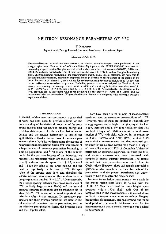
Fig. 1. Experimental arrangement of the target and detector system and the circuit block diagram.

2. EXPERIMENTAL DETAILS

JAERI 120 MeV electron linear accelerator (Take- koshi et al., 1975) is used as a pulsed neutron source. The neutron producing target is a stack of tantalum plates cooled with circulating water. The total thickness of the tantalum is 40mm, which is about 10.5 radiation length and is enough to dissipate most of the electron energy. The target was associated with a moderator which enhances the low energy part of the neutron spectrum. The moderator, covering the target, consists of 200mm diameter × 10mm thick water canned with aluminium and a 40 mm thick polyethylene containing 6.5 wt~ boric acid. The boric acid was added to reduce the number of 2.2 MeV neutron capture ~-rays produced by a neutron capture in hydrogen. For a very thick moderator the neutron spectrum in the low energy region has a neutron energy dependence close to 1/E, while it is E-°"74 for the present moderator (Ohkubo, 1976). The transmission measurements were carried out with a detector at the 190 m flight path station. Experimental geometry is shown in Fig. 1 along with the block diagram of electronic circuits employed. The neutron flight tube was made of aluminium and was filled with helium at 1 atm to reduce the attenuation of neutrons. Seven collimators, made of equal weight paraffin and boric acid, were placed in the tube. A boral plate was located 6.4 m from the neutron producing target to

prevent overlap of low energy neutrons from one linac burst to the next.

The neutron detector consists of 7 sets of 6Li- loaded glass scintillators (NE908, 4 3/4" diameter x 1/2" thick) mounted on photomultipliers (EM19579B). Its detection efficiency is about 10~o for a 1 keV neutron, and the timing uncertainty for the detection of a neutron is several ns, which is negligibly small compared to other time uncertainties. Sig- nals from the photomultipliers were mixed and sent via an emitter follower to a main amplifier in the computer room through a double shielded balloon type coaxial cable 250 m long. The amplitudes of the signals were adjusted by a potentiometer through which a high voltage was supplied to each phototube. The detector was surrounded by a neutron shield of paraffin and boric acid, and the inner surface of the shield was lined with B4C 2 cm thick. The neutron flux was monitored with a 6Li-glass scintillator (NE 905, 1/2" diameter x 1/8" thick) located at about 9 m from the neutron producing target along the 190 m flight tube, about 1 m upstream from a sample changer. Signals from the neutron monitor were fed to a scaler through a time-gate circuit and were sent to a computer. The gate width was adjusted so that the signals of the neutrons with the energies covered by the measurement passed through it.

The signals from the main detector are fed to a time

Neutron resonance parameters of 238U 27

L~..I UNE PRIN'IER L _ , linII/IecPRINTER IICONTROL Jl

64 K words, 154 KHz

MAGNETIC TAPE t , [ 9 trackl. 800BPI t MAGN£TI(~ ' L

MAGNETIC 8001[IPI r s r ~ , , , TAPE L ITA~ CON mOU, I'

-

TOF UNIT t1__ 16 g oh. (Toehlbo)

oh. l( J'AERI )

CORE MB4ORY UNIT 16 K words

~O+pori~ +lXOtect )bit=/word menory cycle = t . 2 ~ o

CRT DISPI_AY~*--~IO~JTANA~ CONTROL[

DIRECT ACCESS CONTROL Data acquisition speed including add-one = 1 .SH, sec

CPU F ~-D Clock : 5 MHz programme interrupt: 4 levels

k- z 8

US(; INTERFACE I I DIGITAL 4PHA-ADC's and 4 TOF UNIT's are I reedlly acceptable _ = ]IO UNIT [evlmt- recording mode including )

I 2 TO | LEVEL INTERRUPT

CONTROL CONTROL

I/O TYPEWRITER

I CONSOLE : I: I ~ P E R r A ~ I -J ,,o h L ,=R I

-I PERFORATOR 1

CARD READER] • -]CONTROL L ICARD READER

J - l~ ' ° °¢ards/min

INCREMENTAL PLOTTER I

, I_.z__..--.._;---~(DIGITAL SIGNALS) I~1 b =u~._ l / u pOVoltoge inputs

I UNtT l=OVoltoge outputs

' 9 Contact inputs

~ C o n t a c t outputs

( l NTERRUPTION ) oContoct inputs

"-----~Voltoge inputs

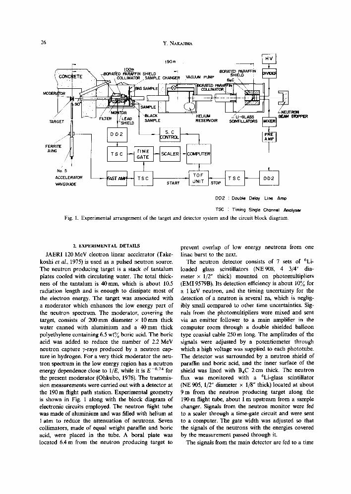
Fig. 2. Schematic diagram of data acquisition and storage system.

anatyser interfaced to a computer (Toshiba ICD-507) which has a core memory of 16 k words of 20 bits/ word, and a cycle time of 1.2Fs (3.0#s with add- one function included). The schematic diagram of a data acquisition and storage system is shown in Fig. 2. Two time analysers are used in this experiment. One of them was made by Toshiba Electric Company Limited. A 10 MHz free-running oscillator is used to derive scaler circuits and provides a minimum channel width of 100 ns, and each of the timing channel widths is a 2 N (N = 0, 1, 2, - - - ,7) multiple of 100 ns. The time analyser can be operated in a so-called accordion mode. The digitized information is fed to the computer through a fast (100 ns) 4-word derando- mizing buffer. The other time analyser was built by the Electronics Shop of JAERI (Kinbara and Tawa, 1974). It has a 80 MHz free-running oscillator which is scaled down to 40 MHz, providing a minimum channel width of 25 ns. The 80 MHz free-running oscillator signal is split into three signals differing by steps of 120 ° in phase. The start pulse, which is random with respect to the oscillator signal, opens gates of flip-flop circuits, of which the 40 MHz output signals are added and fed to the clock scaling circuit. The time jitter relative to the start pulse is reduced to only 4.5 ns. It also possesses a fast (25 ns) 4-word de- randomizing buffer and is operated in the accordion mode.

The energy E (in eV) of a neutron, which takes t/~s

to pass through L m, is given by

(# E = 5226.7 ,

from which the energy resolution is calculated as

A E / E = 2((,St~t) 2 + (AL/L)2) 1/2

= 2L/t((At) 2 + (AL/v)2)I/2/L

= O.028E1/2R,

where At is the full width at half maximum of the total time uncertainty, AL the uncertainty in the flight path length, v the neutron velocity and R = ((At) 2 + (AL/v)2)~/2/L. The time uncertainties are composed of the following factors:

(a) The electron burst width, (b) The time spread due to the moderation process

of the fast photoneutrons, (c) The thickness of the scintillator, (d) The time jitter of the signals in the electronic

circuits, and (e) The channel width of the time analyser.

The time uncertainty introduced by the moderation process in a thick slab of hydrogeneous materials depends on the geometrical shape of the moderator and the initial and final energy of the neutrons. It is proportional to I /E or 1/v, and can be expressed as an uncertainty in the flight path length, of which the full

28 Y. NAKAJIMA

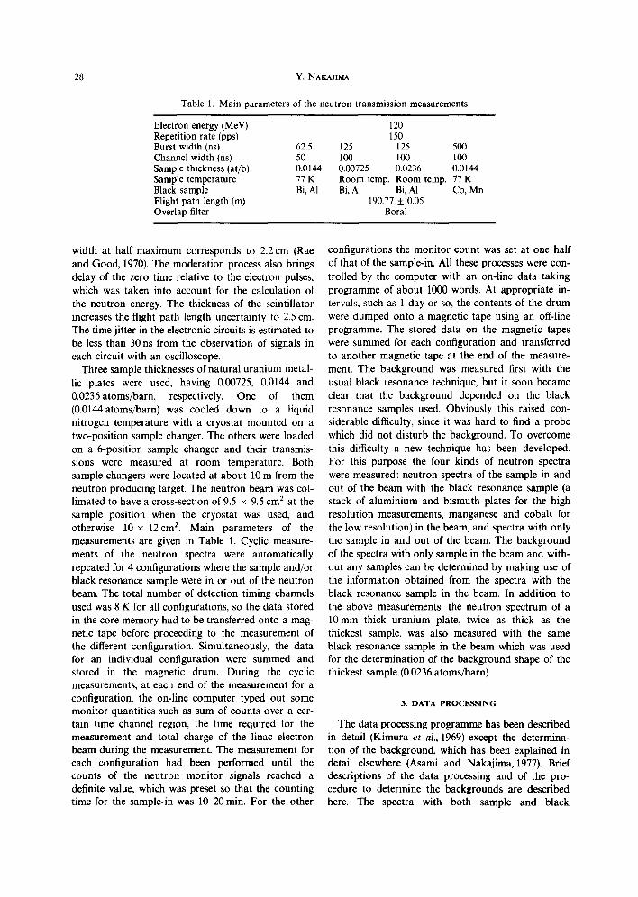
Table 1. Main parameters of the neutron transmission measurements

Electron energy (MeV) 120 Repetition rate (pps) 150 Burst width (ns) 62.5 125 125 500 Channel width (ns) 50 100 100 100 Sample thickness (at/b) 0.0144 0.00725 0.0236 0.0144 Sample temperature 77 K Room temp. Room temp. 77 K Black sample Bi, AI Bi, AI Bi, A1 Co, Mn Flight path length (m) 190.77 _+ 0.05 Overlap filter Boral

width at half maximum corresponds to 2.2 cm (Rae and Good, 1970). The moderation process also brings delay of the zero time relative to the electron pulses, which was taken into account for the calculation of the neutron energy. The thickness of the scintillator increases the flight path length uncertainty to 2.5 cm. The time jitter in the electronic circuits is estimated to be less than 30 ns from the observation of signals in each circuit with an oscilloscope.

Three sample thicknesses of natural uranium metallic plates were used, having 0.00725, 0.0144 and 0.0236 atoms/barn, respectively. One of them (0.0144atoms/barn) was cooled down to a liquid nitrogen temperature with a cryostat mounted on a two-position sample changer. The others were loaded on a 6-position sample changer and their transmissions were measured at room temperature. Both sample changers were located at about 10 m from the neutron producing target. The neutron beam was col- limated to have a cross-section of 9.5 x 9.5 cm 2 at the sample position when the cryostat was used, and otherwise 10 x 12cm 2. Main parameters of the measurements are given in Table 1. Cyclic measurements of the neutron spectra were automatically repeated for 4 configurations where the sample and/or black resonance sample were in or out of the neutron beam. The total number of detection timing channels used was 8 K for all configurations, so the data stored in the core memory had to be transferred onto a magnetic tape before proceeding to the measurement of the different configuration. Simultaneously, the data for an individual configuration were summed and stored in the magnetic drum. During the cyclic measurements, at each end of the measurement for a configuration, the on-line computer typed out some monitor quantities such as sum of counts over a cer- tain time channel region, the time required for the measurement and total charge of the linac electron beam during the measurement. The measurement for each configuration had been performed until the counts of the neutron monitor signals reached a definite value, which was preset so that the counting time for the sample-in was 10-20 min. For the other

configurations the monitor count was set at one half of that of the sample-in. All these processes were con- trolled by the computer with an on-line data taking programme of about 1000 words. At appropriate intervals, such as 1 day or so, the contents of the drum were dumped onto a magnetic tape using an off-line programme. The stored data on the magnetic tapes were summed for each configuration and transferred to another magnetic tape at the end of the measurement. The background was measured first with the usual black resonance technique, but it soon became clear that the background depended on the black resonance samples used. Obviously this raised con- siderable difficulty, since it was hard to find a probe which did not disturb the background. To overcome this difficulty a new technique has been developed. For this purpose the four kinds of neutron spectra were measured: neutron spectra of the sample in and out of the beam with the black resonance sample (a stack of aluminium and bismuth plates for the high resolution measurements, manganese and cobalt for the low resolution) in the beam, and spectra with only the sample in and out of the beam. The background of the spectra with only sample in the beam and without any samples can be determined by making use of the information obtained from the spectra with the black resonance sample in the beam. In addition to the above measurements, the neutron spectrum of a 10mm thick uranium plate, twice as thick as the thickest sample, was also measured with the same black resonance sample in the beam which was used for the determination of the background shape of the thickest sample (0.0236 atoms/barn).

3. DATA PROCESSING

The data processing programme has been described in detail (Kimura et al., 1969) except the determination of the background, which has been explained in detail elsewhere (Asami and Nakajima, 1977). Brief descriptions of the data processing and of the pro- cedure to determine the backgrounds are described here. The spectra with both sample and black


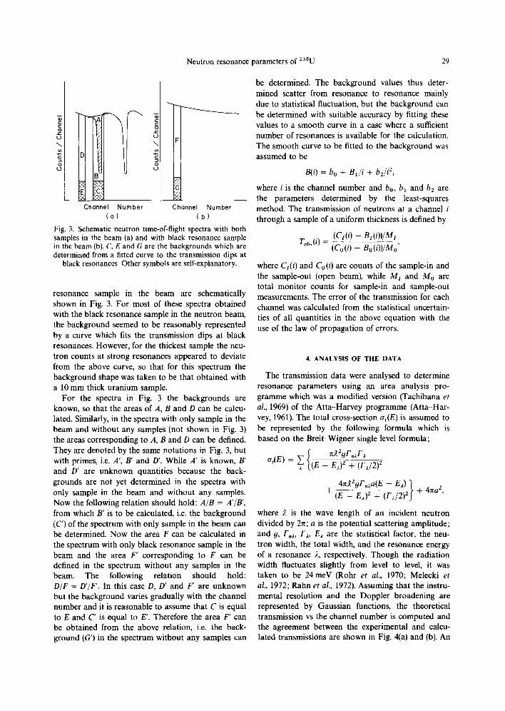
F \

c

0 (..)

E G

Channel Number Channel Number ( a ) ( b )

Fig. 3. Schematic neutron time-of-flight spectra with both samples in the beam (a) and with black resonance sample in the beam (b). C, E and G are the backgrounds which are determined from a fitted curve to the transmission dips at

black resonances. Other symbols are self-explanatory.

resonance sample in the beam are schematically shown in Fig. 3. For most of these spectra obtained with the black resonance sample in the neutron beam, the background seemed to be reasonably represented by a curve which fits the transmission dips at black resonances. However, for the thickest sample the neutron counts at strong resonances appeared to deviate from the above curve, so that for this spectrum the background shape was taken to be that obtained with a 10 mm thick uranium sample.

For the spectra in Fig. 3 the backgrounds are known, so that the areas of A, B and D can be calculated. Similarly, in the spectra with only sample in the beam and without any samples (not shown in Fig. 3) the areas corresponding to A, B and D can be defined. They are denoted by the same notations in Fig. 3, but with primes, i.e. A', B' and D'. While A' is known, B' and D' are unknown quantities because the backgrounds are not yet determined in the spectra with only sample in the beam and without any samples. Now the following relation should hold: A/B = A'/B', from which B' is to be calculated, i.e. the background (C') of the spectrum with only sample in the beam can be determined. Now the area F can be calculated in the spectrum with only black resonance sample in the beam and the area F' corresponding to F can be defined in the spectrum without any samples in the beam. The following relation should hold: D/F = D'/F'. In this case D, D' and F' are unknown but the background varies gradually with the channel number and it is reasonable to assume that C is equal to E and C' is equal to E!. Therefore the area F' can be obtained from the above relation, i.e. the background (G') in the spectrum without any samples can

be determined. The background values thus determined scatter from resonance to resonance mainly due to statistical fluctuation, but the background can be determined with suitable accuracy by fitting these values to a smooth curve in a case where a sufficient number of resonances is available for the calculation. The smooth curve to be fitted to the background was assumed to be

B(i) = bo + B1/i + b2/i 2,

where i is the channel number and bo, bl and b2 are the parameters determined by the least-squares method. The transmission of neutrons at a channel i through a sample of a uniform thickness is defined by

(CI(i) - B1(i))/Mt Tob~ (i) =

(Co (i) - B o (i))/Mo'

where Ct(i) and Co(i) are counts of the sample-in and the sample-out (open beam), while Mx and Mo are total monitor counts for sample-in and sample-out measurements. The error of the transmission for each channel was calculated from the statistical uncertainties of all quantities in the above equation with the use of the law of propagation of errors.

4. ANALYSIS OF THE DATA

The transmission data were analysed to determine resonance parameters using an area analysis programme which was a modified version (Tachibana et al., 1969) of the Atta-Harvey programme (Atta-Har- vey, 1961). The total cross-section af(E) is assumed to be represented by the following formula which is based on the Breit-Wigner single level formula;

n~2gF..~Fa fit(E)

~ (E - Ea) 2 + (ra/2) 2

41t~2gF,~a(E -_ Ea) ~ + (E - E.~) 2 + (F~/2)2J + 47ta2'

where ;~ is the wave length of an incident neutron divided by 2n; a is the potential scattering amplitude; and g, F.a, Fx, Ea are the statistical factor, the neutron width, the total width, and the resonance energy of a resonance ~., respectively. Though the radiation width fluctuates slightly from level to level, it was taken to be 24meV (Rohr et al., 1970; Melecki et al., 1972; Rahn et al., 1972). Assuming that the instru- mental resolution and the Doppler broadening are represented by Gaussian functions, the theoretical transmission vs the channel number is computed and the agreement between the experimental and calculated transmissions are shown in Fig. 4(a) and (b). An

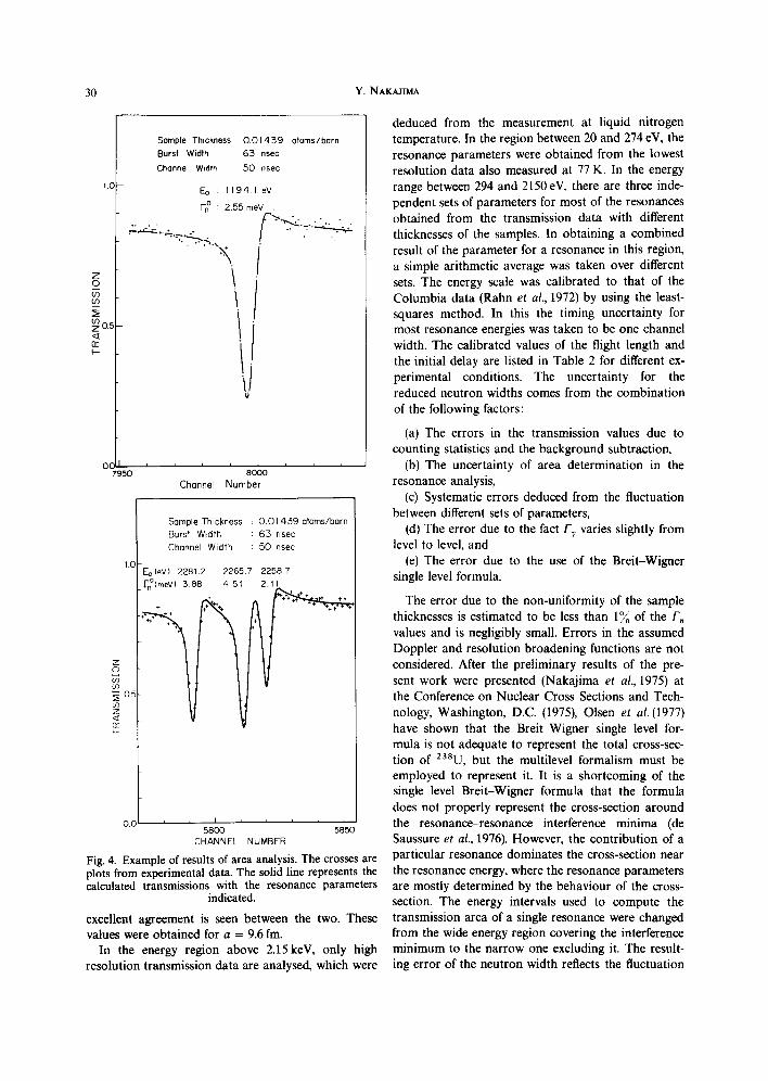
30 Y. NAKAJIMA

I.C

O.C 7950

Sample Thickness : 0 . 0 1 4 3 9 atoms/born

Burst Width : 63 nsec

Channel Width : 50 nsec

Eo : I I 9 4 . 1 eV

I-n ° : 2.55meV .

÷+ ÷ ~ ++ + , -"\ [

/ -i ,j

Z 0

O3

~ 0 . 5

Or" I'-

z o

0.5 (/3 Z

Oz

i i i [ i i i

8 O O O

Channel Number

Sample Thickness : 0 . 0 1 4 3 9 atoms/barn [ Burst Width : 63 nsec

Channel Width : 50 nsec

I'O[-E o (eV) 2281.2 2265.7 2258.7

LF.°I meVl 388 451 2.11

5800 CHANNEL NUMBER

5 8 5 0

Fig. 4. Example of results of area analysis. The crosses are plots from experimental data. The solid line represents the calculated transmissions with the resonance parameters

indicated.

excellent agreement is seen between the two. These values were obtained for a = 9.6 fm.

In the energy region above 2.15keV, only high resolution transmission data are analysed, which were

deduced from the measurement at liquid nitrogen temperature. In the region between 20 and 274 eV, the resonance parameters were obtained from the lowest resolution data also measured at 77 K. In the energy range between 294 and 2150 eV, there are three inde- pendent sets of parameters for most of the resonances obtained from the transmission data with different thicknesses of the samples. In obtaining a combined result of the parameter for a resonance in this region, a simple arithmetic average was taken over different sets. The energy scale was calibrated to that of the Columbia data (Rahn et al., 1972) by using the least- squares method. In this the timing uncertainty for most resonance energies was taken to be one channel width. The calibrated values of the flight length and the initial delay are listed in Table 2 for different experimental conditions. The uncertainty for the reduced neutron widths comes from the combination of the following factors:

(a) The errors in the transmission values due to counting statistics and the background subtraction,

(b) The uncertainty of area determination in the resonance analysis,

(c) Systematic errors deduced from the fluctuation between different sets of parameters,

(d) The error due to the fact Fr varies slightly from level to level, and

(e) The error due to the use of the Breit-Wigner single level formula.

The error due to the non-uniformity of the sample thicknesses is estimated to be less than 1% of the F, values and is negligibly small. Errors in the assumed Doppler and resolution broadening functions are not considered. After the preliminary results of the present work were presented (Nakajima et al., 1975) at the Conference on Nuclear Cross Sections and Tech- nology, Washington, D.C. (1975), Olsen et al. (1977) have shown that the Breit-Wigner single level formula is not adequate to represent the total cross-section of 2~8U, but the multilevel formalism must be employed to represent it. It is a shortcoming of the single level Breit-Wigner formula that the formula does not properly represent the cross-section around the resonance-resonance interference minima (de Saussure et al., 1976). However, the contribution of a particular resonance dominates the cross-section near the resonance energy, where the resonance parameters are mostly determined by the behaviour of the cross- section. The energy intervals used to compute the transmission area of a single resonance were changed from the wide energy region covering the interference minimum to the narrow one excluding it. The result- ing error of the neutron width reflects the fluctuation

Neutron resonance parameters of 23sU

Table 2. Flight path length and initial delay obtained by the least-squares method

Sample thickness Initial delay Flight path length Channel width (at/b) (/as) (m) (ns)

0.0144 -0.835 190.701 400 0.00725 and 0.236 -0.702 190.738 100

0.0144 -0.832 190.922 50

31

of the value due to the above mentioned analysis. Therefore the multilevel effects are considered to be within the quoted error.

5. RESULTS AND DISCUSSION

The resonance parameters of 180s-wave levels in 23su were obtained using the area analysis of the transmission data up to 4.7 keV. The results of these analyses are given in Table 3. Below 1.6 keV neutron energy some resonances, which were assigned to be p-wave resonances by the previous experiment (Corvi et al., 1975), were excluded from the Table.

5.1. Statistical properties

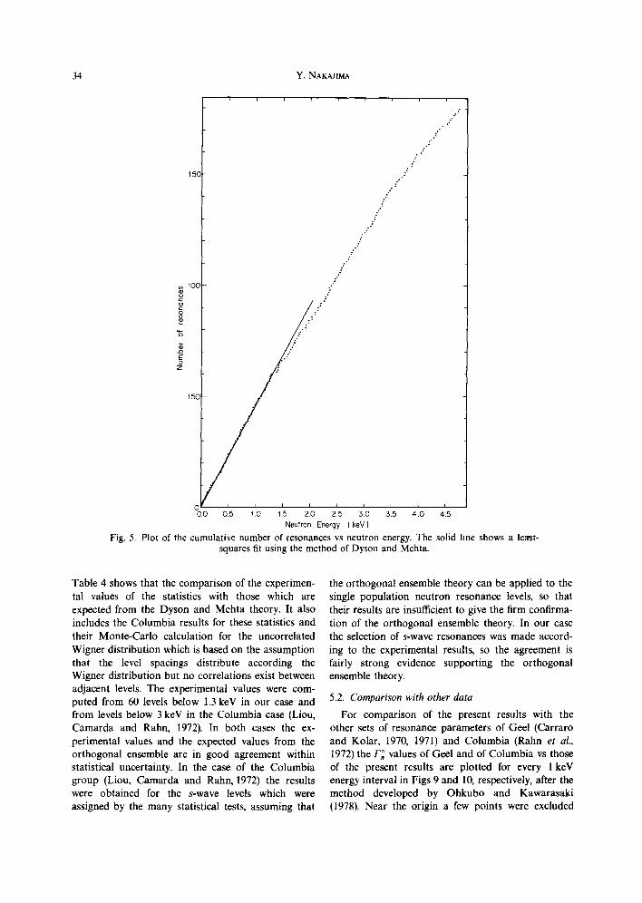
A plot of the cumulative number of resonances vs neutron energy is shown in Fig. 5. The slope of the plot in Fig. 5 is nearly constant up to 1.3 keV, which means that the number of the missed s-wave resonances and the inclusion of the p-wave resonances, or the spurious levels, is small. In this energy range the observed s-wave average level spacing is obtained from the mean slope of the plot in Fig. 5 to be

= 21.9 _+ 1.5 eV.

The departure of the cumulative curve N(E) from the straight line above 1.3 keV indicates that a number of resonances were missed due to the finite resolution of the spectrometer.

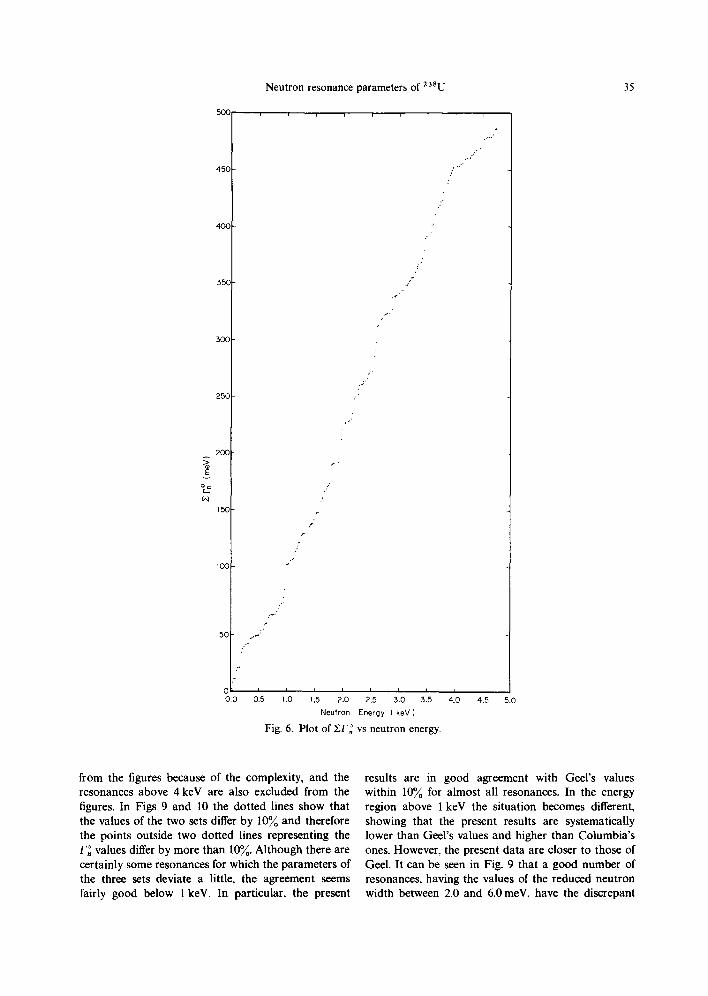
Figure 6 shows the plot of 5~F, ~ vs neutron energy. The mean slope of the plot gives the s-wave strength function as

So = (1.13 +_ 0.13) x 10 -4

up to 4 keV neutron energy. The s-wave strength function thus determined is insensitive to inclusion of p-wave resonances. The average reduced neutron width can be calculated as

F ° = 2.47 _+ 0.33 meV

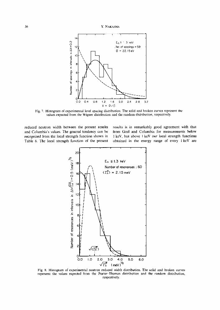
from the s-wave strength function and the average level spacing. Figure 7 shows histograms of experimental level spacings up to 1.3 keV, in comparison

with the curve expected from the Wigner distribution;

Pw(x) = nx/2 exp( - nx2/4),

where x = D/D. It can be seen that the Wigner distribution is in better agreement with the experimental one than the random distribution, and the difference between the experimental histograms and the Wigner distribution can be explained by statistical fluctuation.

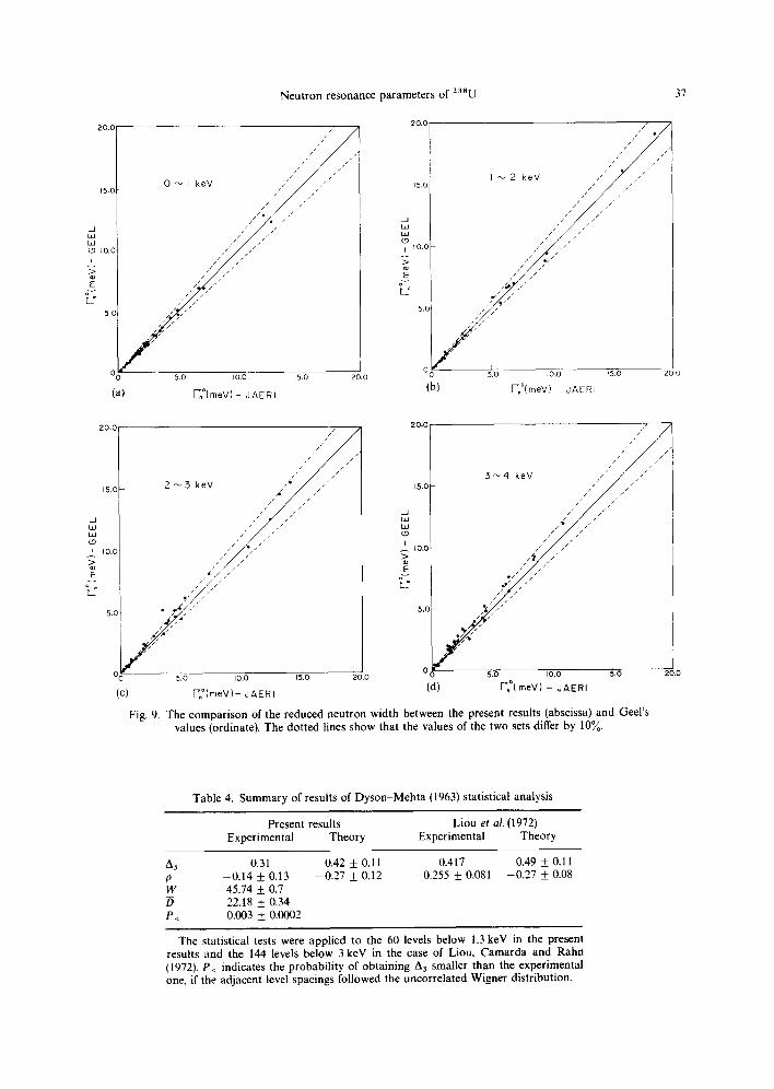
In Fig. 8 is shown histograms of experimental values of the neutron reduced width up to 1.3 keV in comparison with the Porter-Thomas distribution:

Pp_ T(X) = (27tX) 1/2 exp(--x/2)

and the random distribution (v = 2)

PR(x) = e x p ( - x )

where x = F°/F~,. The Porter-Thomas distribution is in better agreement with the experimental histograms, while the difference between the histograms of the experimental values and the Porter-Thomas distribution may most likely be due to statistical fluctuation. The maximum likelihood method (Porter and Thomas, 1956) was applied to the distribution of the neutron reduced width below 1.3 keV to determine the number of degrees of freedom of the chi-squared distribution which gives the best fit to the data, along with an estimate of the error. Though the result v = 1.25 + 0.17 is not inconsistent with the Porter- Thomas distribution, it indicates the lack of the small resonances or the statistical fluctuation if the Porter- Thomas distribution (v = 1) is a good representation of the neutron reduced width distributions.

The Wigner distribution was proved to be very close to the results of the accurate analytical and nu- merical calculations (Blumberg and Porter, 1958; Rosenzweig, 1958; Porter and Rosenzweig, 1960; Mehta, 1960; Gaudin, 1961) using a Gaussian ensemble where the matrix elements are independently distributed according to Gaussian laws with zero mean, the variance of the distribution of the diagonal elements being twice that for the non-diagonal elements. The validity of the Wigner distribution has been confirmed experimentally many times, Dyson and Mehta proposed an orthogonal ensemble

32 Y. NAKAJIMA

(Dyson, 1962a; Dyson, 1962b; Dyson, 1962c; Dyson and Mehta, 1963) where the nuclear levels are eigen- values of a random symmetric unitary matrix. The orthogonal ensemble was introduced on the basis of a more natural assumption of the matrix elements than the Gauss±an ensemble. The statistical analysis of Dyson and Mehta (1963) has been applied to our data

in an attempt to test the validity of the orthogonal ensemble. The first statistic is the mean square devi- ation of the staircase plots of cumulative number of levels as a function of energy from the straight line

and is defined for a sequence of observed resonance

where 2L indicates the range of the observed energy interval with the origin of the energy in the centre, N ( E ) is the number of levels having energy between 0 and E, and, for negative E, minus the number of levels between E and 0, and A and B are chosen so that the straight line y = A E + B gives the minimum value of Aa. The statistic A3 is a measure of the long range correlation of the level spacings. For the orthogonal ensemble, Dyson and Mehta have shown that

A 3 = (1/~ 2) (In n - 0.0687) and var ( A 3 ) = (0.11) 2.

The second one is the correlation coefficient for adjacent nearest neighbour level spacings, which is

energies by

{; } A3 = Min ( N ( E ) - A E - B) 2 d E , A,B -L

defined by

p(Di , Di + 1) =

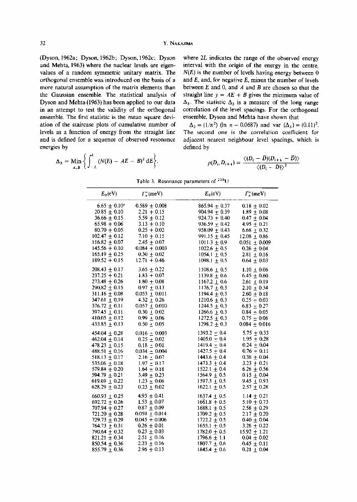
Table 3. Resonance parameters of 238U

<(D~ - D)(Di+ 1 - 13)>

Eo(eV) r~(meV) Eo(eV) F~(meV)

___ 0.10 a 0.589 _ 0.008 865.94 + 0.37 0.18 ___ 0.02 ___ 0.10 2.21 + 0.15 904.94 + 0.39 1.89 + 0.08 + 0.15 5.59 ___ 0.12 924.73 + 0.40 0.47 + 0.04 + 0.06 3.13 + 0.10 936.59 + 0.42 4.95 + 0.21 + 0.05 0.25 + 0.02 958.09 + 0.43 6.68 + 0.32 ___ 0.12 7.10 ± 0.15 991.15 ± 0.45 12.08 ± 0.86 ± 0.07 2.45 ± 0.07 1011.3 ± 0.9 0.051 ± 0.009 ± 0.10 0.084 ± 0.003 1022.6 + 0.5 0.26 ± 0.04 ± 0.25 0.30 ___ 0.02 1054.1 ± 0.5 2.81 ± 0.16 ± 0.15 12.71 ± 0.46 1098.1 ± 0.5 0.64 ± 0.03

± 0.17 3.65 + 0.22 1108.6 + 0.5 1.10 ± 0.06 ± 0.21 1.83 ± 0.07 1139.8 ± 0.6 6.45 ± 0.60 ± 0.26 1.80 ± 0.08 1167.2 ± 0.6 2.61 ___ 0.19 ± 0.15 0.97 ± 0.13 1176.7 ± 0.3 2.10 ± 0.34 ± 0.08 0.053 ± 0.011 1194.4 ± 0.3 2.60 ± 0.18 _ 0.19 4.32 + 0.26 1210.6 ± 0.3 0.25 ± 0.03 ± 0.11 0.057 ± 0.010 1244.5 ± 0.3 6.83 ± 0.27 ± 0.11 0.30 ± 0.02 1266.6 ± 0.3 0.84 ± 0.05 _ 0.12 0.99 ___ 0.06 1272.5 ± 0.3 0.75 + 0.06 ± 0.13 0.50 ± 0.05 1298.2 ± 0.3 0.084 ± 0.016

± 0.28 0.016 ± 0.003 1393.2 ± 0.4 5.75 + 0.33 ± 0.14 0.25 + 0.02 1405.0 ± 0.4 1.95 ± 0.28 ± 0.15 0.18 + 0.01 1419.4 ± 0.4 0.24 ± 0.04 ± 0.16 0.034 ± 0.004 1427.5 ± 0.4 0.76 ± 0.11 ± 0.17 2.16 ± 0.07 1443.6 ± 0.4 0.38 ± 0.04 ± 0.18 1.97 + 0.17 1473.3 ± 0.4 3.23 ± 0.21 ± 0.20 1.64 ± 0.18 1522.1 ± 0.4 6.26 + 0.56 _ 0.21 3.49 ± 0.23 1564.9 __+ 0.5 0.15 _ 0.04 + 0.22 1.23 ± 0.06 1597.3 + 0.5 9.45 ± 0.93 + 0.23 0.23 + 0.02 1622.1 ± 0.5 2.57 ± 0.28

± 0.25 4.93 ± 0.41 1637.4 ___ 0.5 1.14 + 0.21 ± 0.26 1.53 ± 0.07 1661.8 ± 0.5 5.10 ± 0.73 ± 0.27 0.87 ± 0.09 1688.1 ± 0.5 2.58 + 0.29 _ 0.28 0.059 ± 0.014 1709.2 ± 0.5 2.17 ± 0.20 ± 0.29 0.045 ± 0.006 1722.2 ± 0.5 0.40 ± 0.04 ± 0.31 0.26 ± 0.01 1655.1 ± 0.5 3.26 ± 0.22 ± 0.32 0.23 + 0.03 1782.0 ± 0.5 15.92 ± 1.21 ± 0.34 2.51 ± 0.16 1796.6 ± 1.1 0.04 ± 0.02 ± 0.36 2.23 + 0.16 1807.7 + 0.6 0.45 + 0.11 ± 0.36 2.96 ± 0.13 1845.4 ± 0.6 0.21 + 0.04

6.65 20.85 36.66 65.98 80.70

102.47 116.82 145.56 165.19 189.52

208.43 237.25 273.48 290.82 311.16 347.61 376.72 397.45 410.05 433.85

454.04 462.04 478.23 488.51 518.13 535.06 579.84 594.79 619.69 628.29

660.93 692.72 707.94 721.20 729.73 764.73 790.64 821.21 850.54 855.79

<(Di - / 3 ) > 2

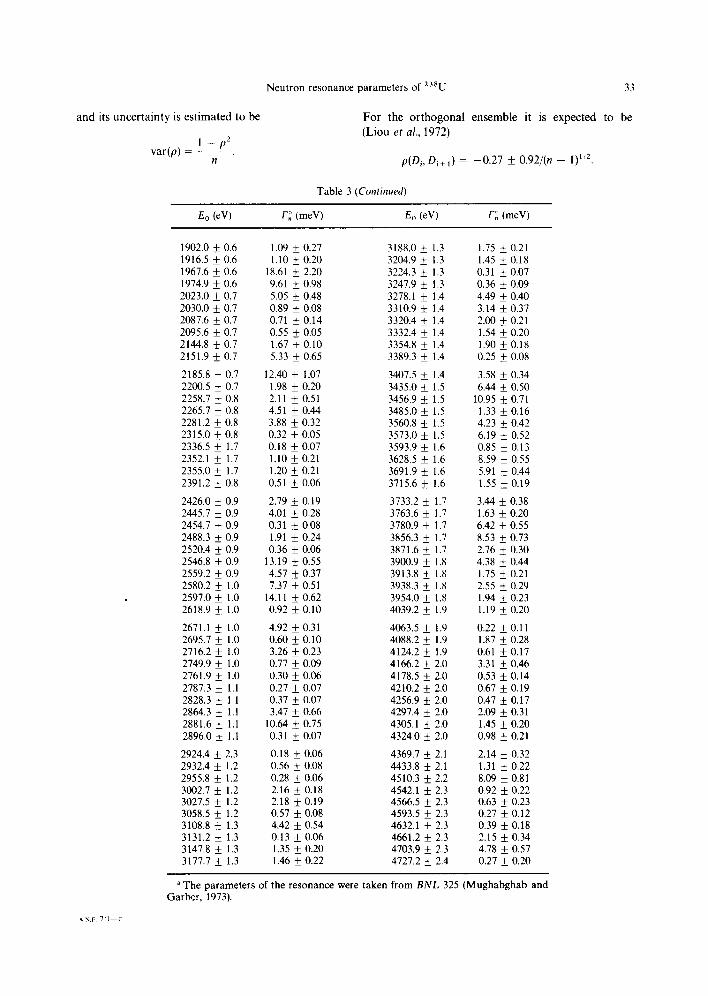
Neutron resonance parameters of 23su 33

a n d its u n c e r t a i n t y is e s t ima ted to be

1 - - p 2 var(p) =

n

Fo r the o r t h o g o n a l e n s e m b l e it is expec ted to be

(Liou et al., 1972)

p(Di, Di+ 1) = - 0 . 2 7 + 0.92/(n - 1) 1/2.

Table 3 (Continued)

Eo (eV) F~ (meV) Eo (eV) f ' , ' (meV)

1902.0 ± 0.6 1.09 ± 0.27 3188.0 _ 1.3 1.75 ± 0.21 1916.5 + 0.6 1.10 + 0.20 3204.9 ± 1.3 1.45 ± 0.18 1967.6 + 0.6 18.61 ± 2.20 3224.3 + 1.3 0.31 + 0.07 1974.9 + 0.6 9.61 ± 0.98 3247.9 + 1.3 0.36 ± 0.09 2023.0 ± 0.7 5.05 ± 0.48 3278.1 ± 1.4 4.49 ± 0.40 2030.0 ± 0.7 0.89 ± 0.08 3310.9 ± 1.4 3.14 + 0.37 2087.6 ± 0.7 0.71 ± 0.14 3320.4 ± 1.4 2.00 ± 0.21 2095.6 ± 0.7 0.55 ± 0.05 3332.4 ± 1.4 1.54 ± 0.20 2144.8 ± 0.7 1.67 ± 0.10 3354.8 ± 1.4 1.90 ± 0.18 2151.9 ± 0.7 5.33 ± 0.65 3389.3 + 1.4 0.25 ± 0.08

2185.8 ± 0.7 12.40 ± 1.07 3407.5 ± 1.4 3.58 ± 0.34 2200.5 ± 0.7 1.98 + 0.20 3435.0 ± 1.5 6.44 ± 0.50 2258.7 ± 0.8 2.11 ± 0.51 3456.9 ± 1.5 10.95 ± 0.71 2265.7 ± 0.8 4.51 ± 0.44 3485.0 ± 1.5 1.33 ± 0.16 2281.2 ± 0.8 3.88 ± 0.32 3560.8 ± 1.5 4.23 ± 0.42 2315.0 ± 0.8 0.32 ± 0.05 3573.0 ± 1.5 6.19 ± 0.52 2336.5 ± 1.7 0.18 ± 0.07 3593.9 ± 1.6 0.85 ± 0.13 2352.1 ± 1.7 1.10 ± 0.21 3628.5 ± 1.6 8.59 ± 0.55 2355.0 ± 1.7 1.20 ± 0.21 3691.9 ± 1.6 5.91 ± 0.44 2391.2 ± 0.8 0.51 ± 0.06 3715.6 ± 1.6 1.55 ± 0.19

2426.0 ± 0.9 2.79 ± 0.19 3733.2 ± 1.7 3.44 ± 0.38 2445.7 +__ 0.9 4.01 ± 0.28 3763.6 ± 1.7 1.63 ± 0.20 2454.7 ± 0.9 0.31 ± 0.08 3780.9 + 1.7 6.42 ± 0.55 2488.3 ± 0.9 1.91 ± 0.24 3856.3 ± 1.7 8.53 _+ 0.73 2520.4 ± 0.9 0.36 ± 0.06 3871.6 ± 1.7 2.76 ± 0.30 2546.8 ± 0.9 13.19 ± 0.55 3900.9 ± 1.8 4.38 ± 0.44 2559.2 ± 0.9 4.57 ± 0.37 3913.8 ± 1.8 1.75 ± 0.21 2580.2 ± 1.0 7.37 ± 0.51 3938.3 ± 1.8 2.55 ± 0.29 2597.0 ± 1.0 14.11 ± 0.62 3954.0 ± 1.8 1.94 ± 0.23 2618.9 ± 1.0 0.92 ± 0.10 4039.2 ± 1.9 1.19 ± 0.20

2671.1 + 1.0 4.92 ± 0.31 4063.5 ± 1.9 0.22 ± 0.11 2695.7 + 1.0 0.60 + 0.10 4088.2 ± 1.9 1.87 ± 0.28 2716.2 ± 1.0 3.26 ± 0.23 4124.2 ± 1.9 0.61 ± 0.17 2749.9 ± 1.0 0.77 ± 0.09 4166.2 ± 2.0 3.31 ± 0.46 2761.9 + 1.0 0.30 ± 0.06 4178.5 ± 2.0 0.53 ± 0.14 2787.3 ± 1.1 0.27 ± 0.07 4210.2 ± 2.0 0.67 ± 0.19 2828.3 ± 1.1 0.37 ± 0.07 4256.9 ± 2.0 0.47 ± 0.17 2864.3 + 1.1 3.47 ± 0.66 4297.4 ± 2.0 2.09 ___ 0.31 2881.6 ± 1.1 10.64 ± 0.75 4305.1 + 2.0 1.45 ± 0.20 2896.0 ± 1.1 0.31 ± 0.07 4324.0 ± 2.0 0.98 ± 0.21

2924.4 ± 2.3 0.18 ± 0.06 4369.7 ± 2.1 2.14 ± 0.32 2932.4 ± 1.2 0.56 ± 0.08 4433.8 ± 2.l 1.31 + 0.22 2955.8 ± 1.2 0.28 ± 0.06 4510.3 + 2.2 8.09 ± 0.81 3002.7 ± 1.2 2.16 ± 0.18 4542.1 + 2.3 0.92 ± 0.22 3027.5 ± 1.2 2.18 ± 0.19 4566.5 ± 2.3 0.63 + 0.23 3058.5 ___ 1.2 0.57 ± 0.08 4593.5 ± 2.3 0.27 ± 0.12 3108.8 ± 1.3 4.42 ± 0.54 4632.1 ± 2.3 0.39 ± 0.18 3131.2 ± 1.3 0.13 ± 0.06 4661.2 ± 2.3 2.15 ± 0.34 3147.8 ± 1.3 1.35 ± 0.20 4703.9 ± 2.3 4.78 + 0.57 3177.7 ± 1.3 1.46 +_ 0.22 4727.2 ± 2.4 0.27 ± 0.20

a The parameters of the Garber, 1973).

resonance were taken from BNL 325 (Mughabghab and

~,.rq.E. 7/1 t"

34 Y. NAKAJIMA

150

100i

=o 8

z

15C

. t "

I O o °?5 ,o ,!5

••°

°.•

l'

_

zJ5 3o 315 41o 4~.5 Neutron Energy (keV)

Fig. 5. Plot of the cumulative number of resonances vs neutron energy. The solid line shows a least- squares fit using the method of Dyson and Mehta.

Table 4 shows that the comparison of the experimental values of the statistics with those which are expected from the Dyson and Mehta theory. It also includes the Columbia results for these statistics and their Monte-Carlo calculation for the uncorrelated Wigner distribution which is based on the assumption that the level spacings distribute according the Wigner distribution but no correlations exist between adjacent levels. The experimental values were computed from 60 levels below 1.3 keV in our case and from levels below 3 keV in the Columbia case (Liou, Camarda and Rahn, 1972). In both cases the experimental values and the expected values from the orthogonal ensemble are in good agreement within statistical uncertainty. In the case of the Columbia group (Liou, Camarda and Rahn, 1972) the results were obtained for the s-wave levels which were assigned by the many statistical tests, assuming that

the orthogonal ensemble theory can be applied to the single population neutron resonance levels, so that their results are insufficient to give the firm confirma- tion of the orthogonal ensemble theory• In our case the selection of s-wave resonances was made according to the experimental results, so the agreement is fairly strong evidence supporting the orthogonal ensemble theory.

5.2. Comparison with other data

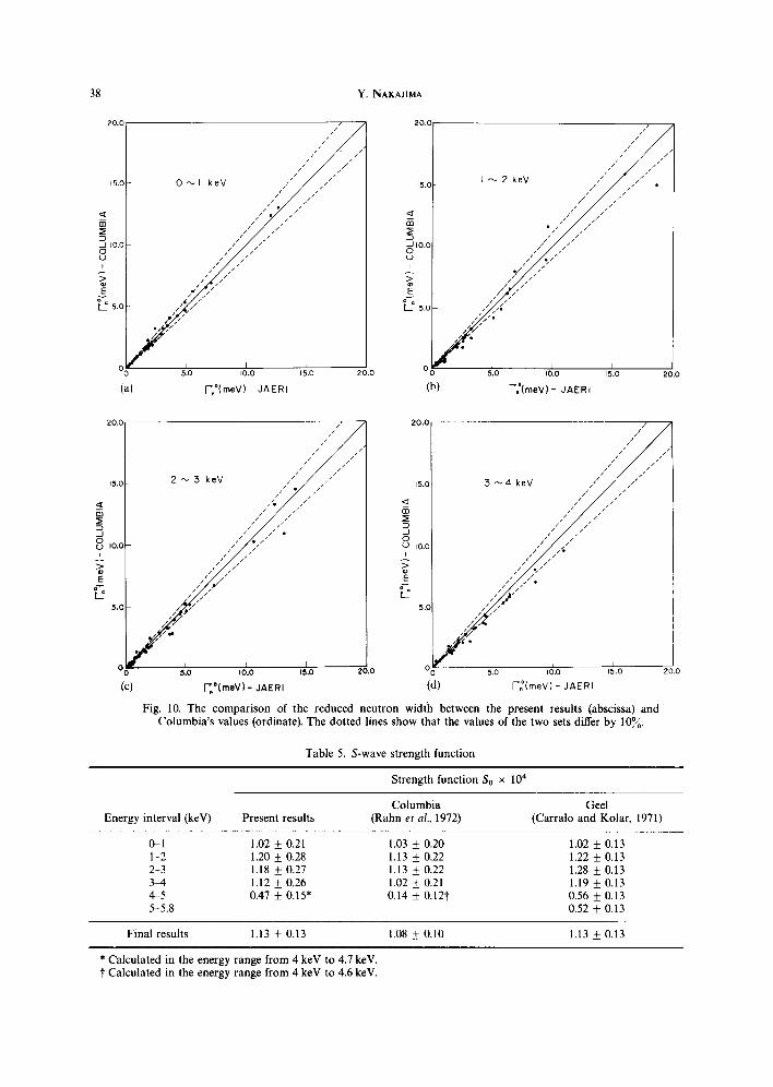
For comparison of the present results with the other sets of resonance parameters of Geel (Carraro and Kolar, 1970, 1971) and Columbia (Rahn et al., 1972) the F~ values of Geel and of Columbia vs those of the present results are plotted for every 1 keV energy interval in Figs 9 and 10, respectively, after the method developed by Ohkubo and Kawarasaki (1978). Near the origin a few points were excluded

Neutron resonance parameters of 2 3 s u 35

500

450

400

55C

300

250

200

150

100

50

0 0.0

f

J

f"

..."

.....'"

. , J

i i 0.5 T.O 1,5 Z.O 2.5 3 0 3 5

Neutron Energy ( k e V )

Fig. 6. Plot of EF~ vs neutron energy.

...."

4.0 4.5 5.0

from the figures because of the complexity, and the resonances above 4 keV are also excluded from the figures. In Figs 9 and 10 the dotted lines show that the values of the two sets differ by 10~o and therefore the points outside two dotted lines representing the F~, values differ by more than 10~o. Although there are certainly some resonances for which the parameters of the three sets deviate a little, the agreement seems fairly good below 1 keV. In particular, the present

results are in good agreement with Geel's values within 10~o for almost all resonances. In the energy region above 1 keV the situation becomes different, showing that the present results are systematically lower than Geel's values and higher than Columbia's ones. However, the present data are closer to those of Geel. It can be seen in Fig. 9 that a good number of resonances, having the values of the reduced neutron width between 2.0 and 6.0 meV, have the discrepant

36 Y. NAKAJIMA

f ? ..... E n <- 1.3 keV

12 No. of spacings = 59 <3 \ D = 2 2 1 1 5 e V

~ ', ~ 8

~ 61- A ",

01 I i I

0.0 0.4 0 8 , 2 ~.6 2.0 2.4 2.8 ~.2

X = D / D

Fig. 7. Histogram of experimental level spacing distribution. The solid and broken curves represent the values expected from the Wigner distribution and the random distribution, respectively.

reduced neutron width between the present results and Columbia's values. The general tendency can be recognized from the local strength function shown in Table 6. The local strength function of the present

results is in remarkably good agreement with that from Geel and Columbia for measurements below 1 keV, but above 1 keV our local strength functions obtained in the energy range of every 1 keV are

2O

> 18

E

~ 16 ~ o II

@ 14 .

<3

~ ~o

.E 8 -I

~ s

g t

\ l l l

En -< 1.3 keY

Number of resononces ; 6 0

<Fn°) = 2 . 1 5 meV

l l l l l l l l

2 V~n> ,..,.

0 0.0 1.0 2.0 3.0 4.0 5.0 6.0

( meV )V2 Fig. 8. Histogram of experimental neutron reduced width distribution. The solid and broken curves represent the values expected from the Porter-Thomas distribution and the random distribution,

respectively.

Neutron resonance parameters of 2 3 8 U 37

20.0

0 ~ I k e V 15.0

w (D IO.C

i / / / / / i / J / / /

E / J

L ~

5.(

o~' 5'o ,o.o

( a ) r.°(meV)- JAERI

j ~ / / . / /

j / , /~

15.0 2 0 . 0

20.0

15.0

g Ld C9

I lO.C

L o

5.0

o o-

I ~ 2 k e V / / / / / "

/ " , zt

1~ j~

I 5'.o ~o.o ,Lo 2, 20.0

(b) r.°(meV)- JAERI

20.0

15.0

LLI (.9

l I 0 . 0

L o

5.C

o~

///

2 ~ 3 keY ,,/6 " ~ /'// ," z ,/

J ~,/ J

j j / i / / j / • / i z

(c) 5.0 I0.0 15.0

F',° ( m e V ) - JAERI

20.0

20,C

15.C

J b.l laJ

I I 0 . 0 >

L o

5.0

0

(d)

3 ~ 4 keV

///// / / / J

//// . / / /I/

,// /~

/i i /

f i I

5.0 io.o 15.0

J'-'.*( m e V ) - JAERI

j

Fig. 9. The comparison of the reduced neutron width between the present results (abscissa) and Geel's values (ordinate). The dotted lines show that the values of the two sets differ by 10%.

20.0

Table 4. Summary of results of Dyson-Mehta (1963) statistical analysis

Present results Liou et al. (1972) Experimental Theory Experimental Theory

A 3 0.31 0.42 + 0.11 0.417 0.49 _+ 0.11 p --0.14 + 0.13 --0.27 -k 0.12 --0.255 + 0.081 --0.27 __+ 0.08 W 45.74 _+ 0.7

22.18 _+ 0.34 P< 0.003 +_ 0.0002

The statistical tests were applied to the 60 levels below 1.3 keV in the present results and the 144 levels below 3 keV in the case of Liou, Camarda and Rahn (1972). P< indicates the probability of obtaining A 3 smaller than the experimental one, if the adjacent level spacings followed the uncorrelated Wigner distribution.

38 Y. NAKAJIMA

20.0

15.o

_1 LO.O 0 0 i

E g.., L ~ 5.0

0(

(a) F'.*( meV ) - JAERI

/ / t

/ / / / / /

0 ~ 1 keY / ' / / / / z

/ / . / / / / / / • / /

/ , / z / / / , / / J

; / / / /

/ /z

7 / j / , 4 , /

/," v / ,#' i /

I 51.0 I0.0 t 5.0 20.0

20.0

15.0

<

(~IO.C (.9 I

E

~_~ 5.C

o~

(b)

. /

L ~ 2 k e Y / / / /

/ / / /

, / j / J • / / / /

/I/ j / , / J

/ / J , / / g

/ , / . z z j /

s.o ,o.o ~s.o 20.0

F' [ (meV) - JAERI

20.0 // //////////~// 15.0 2 ~ 5 keY /,,

/ J j /

_10 / ' • J / • (..) 10.0 / /

E j , / j / "

L © / / / 5 , c ,, / / 7P

, / / /

I I I o~, 5.0 ,oo ,5.0 20.0

(c) ~ * ( r n e V l - JAERI

20.0

15.0

I0.0 i

L o

5.£

o~

/ i J

/ •

J /

J J

5 ~ 4 keV / / J / / J j /

J . / /" / J

z /z /" , / / /

/ oJ / J

/ / , / •

j J ~ / , / /

L 5.0 I0.0 15,0 20.0

(d) I - '~ (meV)- JAERI

Fig. 10. The comparison of the reduced neutron width between the present results (abscissa) and Columbia's values (ordinate). The dotted lines show that the values of the two sets differ by 10%.

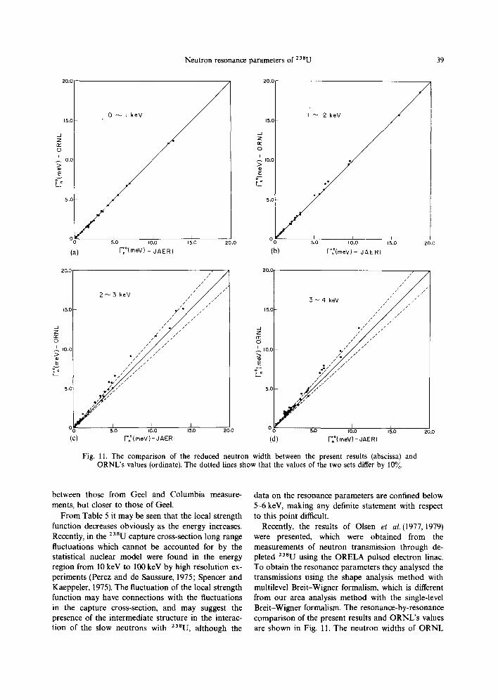
Table 5. S-wave strength function

Strength function So x 104

Columbia Geel Energy interval (keV) Present results (Rahn et al., 1972) (Carralo and Kolar, 1971)

0-1 1.02 + 0.21 1.03 + 0.20 1.02 ___+ 0.13 1-2 1.20 + 0.28 1.13 + 0.22 1.22 -t- 0.13 2 -3 1.18 4- 0.27 1.13 _____ 0.22 1.28 + 0.13 3 4 1.12 + 0.26 1.02 _____ 0.21 1.19 + 0.13 4 - 5 0.47 + 0 .15" 0.14 + 0.121" 0.56 4- 0.13 5-5.8 0.52 _____ 0.13

Final results 1.13 4- 0.13 1.08 + 0.10 1.13 + 0.13

* Calculated in the energy range from 4 keV to 4.7 keV. 1" Calculated in the energy range from 4 keV to 4.6 keV.


20.0

15,0

J z

0 I

I0,0

E g~ L ~

5.0

20.0

15.0

0

10.0 >

t 2

5.0

..... 20.0

I I O~ O~ 51.0 I0.0 15.0 20.0

(a) 7 . ° (meV) - JAERI (b)

15 .0

--I Z

0 I

I0.0 >

b

5.0 ̧

I I I 5.0 io.o ,5.o zo.o

F'."(meV)- J A E R I

/ / / " 2 ~ 5 k e V Y " / , " "

/ J / / / /

/ , / / /

e/~, / j ,4 .,/

20.0

15.0

.d Z tic 0 I I 0 . 0

E L ~

5.0

o~ so ,0.0 ,5.0 20.0 o j (c) ["*(meV ) - JAERI (d)

/ /

5 ~ 4 k e V

e~ ~ / / /

I 5.0 io.o 15.o ~.o

I".*( meV ) - J A E R I

Fig. 11. The comparison of the reduced neutron width between the present results (abscissa) and ORNL's values (ordinate). The dotted lines show that the values of the two sets differ by 10%.

between those from Geel and Columbia measurements, but closer to those of Geel.

From Table 5 it may be seen that the local strength function decreases obviously as the energy increases. Recently, in the 23aU capture cross-section long range fluctuations which cannot be accounted for by the statistical nuclear model were found in the energy region from 10 keV to 100 keV by high resolution ex- periments (Perez and de Saussure, 1975; Spencer and Kaeppeler, 1975). The fluctuation of the local strength function may have connections with the fluctuations in the capture cross-section, and may suggest the presence of the intermediate structure in the interac- tion of the slow neutrons with 238U, although the

data on the resonance parameters are confined below 5-6 keV, making any definite statement with respect to this point difficult.

Recently, the results of Olsen et al.(1977, 1979) were presented, which were obtained from the measurements of neutron transmission through de- pleted 238U using the ORELA pulsed electron linac. To obtain the resonance parameters they analysed the transmissions using the shape analysis method with multilevel Breit-Wigner formalism, which is different from our area analysis method with the single-level Breit-Wigner formalism. The resonance-by-resonance comparison of the present results and ORNL's values are shown in Fig. 11. The neutron widths of ORNL

40 Y. NAKAJIMA

are in good agreement with our results below 2 keV, but above 2keV are systematically larger than our results by about 10~o on average. The reasons for these discrepancies cannot be given easily, but it is not likely that the discrepancies are due to the difference of the resonance formalisms because the magni- tude of the level-level interference term is not proportional to the neutron width (de Saussure et al., 1976).

Acknowledgement~The authors wish to thank Drs A. Asami, M. Mizumoto, T. Fuketa, and H. Takekoshi for their participation in the experiment and useful discussions.

We are grateful to Professor T. Terasawa (University of Tokyo) for useful discussions and comments. We also thank the operating group of the JAERI linac for the stable operation of the accelerator for a long period.

REFERENCES

Asami S. and Nakajima Y. (1977) Nucl. Instrum. Meth. 147, 577.

Atta A. E. and Harvey J. A. (1961) ORNL-3205. Blumberg S. and Porter C. E. (1958) Phys. Rev. 110, 786. Carraro G. and Kolar W. (1970) Proc. 2nd Int. Conf. Nucl.

Data for Reactors, Helsinki, Vol. I, p. 403. Carraro G. and Kolar W. (1971) Proc. 3rd Conj'. Neutron

Cross Sections and Technol. Knoxville, Vol. 2, p. 701. Corvi F., Rohr G. and Weigman H. (1975) Proc. Conj'.

Nucl. Cross Sections and Technology, Washington, D.C., Vol. II, p. 733.

de Saussure G. et al. (1976) Nucl. Sci. Engng 61,496. Dyson F. J. (1962a) d. Math. Phys. 3, 140. Dyson F. J. (1962b) J. Math. Phys. 3, 157. Dyson F. J. (1962c) d. Math. Phys. 3, 166.

Dyson F. J. and Mehta M. L. (1963) J. Math. Phys. 4, 701. Garg J. B. et al. (1964) Phys. Rev. 134, B985. Gaudin M. (1961) Nucl. Phys. 25, 447. Kimura E. et al. (1969) J A E R l - - m e m o 3398. Kimbara S. and Tawa F. (1974) JAERI -M 5835. In

Japanese. Liou H. I. et al. (1972) Phys. Rev. C5, 974. Liou H. I., Camarda H. S. and Rahn F. (1972) Phys. Rev.

C5, 1002. Malecki H. et al. (1972) Atom Energy 32, 49. Mehta M. L. (1960) Nucl. Phys. 18, 385. Mughabghab S. F. and Garber D. I. (1973) Neutron Cross-

Sections, Vol. I. Resonance Parameters, BNL-325, 3rd Edn.

Nakajima Y. et al. (1975) Proc. Conf. Nucl. Cross Sections and Technol., Washington, D.C., Vol. II, p. 738.

Ohkubo M. (1976) JAERI -M 6630. In Japanese. Ohkubo M. and Kawarasaki Y. (1978) JAERI 7545. Olsen D. K. et al. (1977) Nucl. Sci. Engng 62, 479. Olsen D. K. et al. (1979) NucL Sci. Enono 69, 202. Perez R. B. and de Saussure G. (1975) Proc. Conf. Nucl.

Cross Sections and Technol. Washington, D.C., Vol. II, p. 623.

Porter C. E. and Thomas R. G. (1956) Phys. Rev. 104, 483. Porter C. E. and Rosenzweig N. (1960) Suomalaisen Tie-

deakatemian Tomituksia (Ann. Acad. Sci. Fennicae) A IV, (441.

Rae E. R. and Good W. M. (1970) Experimental Neutron Resonance Spectroscopy (edited by Harvey J. A.), Aca- demic Press, New York, p. 2.

Rahn F. et al. (1972) Phys. Rev. C6, 1854. Rosenzweig N. (1958) Phys. Rev. Lett. 1, 24. Rohr G., Weigman H. and Winter J. (1970) Proc. 2nd Int.

Conf. Nucl. Data for Reactors, Helsinki, Vol. I, p. 413. Spencer R. R. and Kaeppeler F. (1975) Proc. Conf. Nucl.

Cross Sections and Technol., Washington, D.C., Vol. II, p. 620.

Tachibana A. et al. (1969) JAERl-memo 3728. Takekoshi H. et al. (1975) JAERI 1238. In Japanese.

Documents

Neutron resonance parameters of 238U