Neutrinos from STORed Muons

Letter of Intent

P. Kyberd and D.R. Smith

Brunel University

L. Coney

University of California, Riverside

S. Pascoli

Institute for Particle Physics Phenomenology, Durham University

C. Ankenbrandt, S.J. Brice, A.D. Brossa, H. Cease, J. Kopp, N. Mokhov,

J. Morfin, D. Neuffer, M. Popovic, P. Rubinov, and S. Striganov

Fermi National Accelerator Laboratory

A. Blondel, A. Bravar, and E. Noah

University of Geneva

R. Bayes and F.J.P. Soler

University of Glasgow

A. Dobbs, K. Long, J. Pasternak, E. Santos, and M.O. Wascko

Imperial College London

S.K. Agarwalla

Instituto de Fisica Corpuscular, CSIC and Universidad de Valencia

a Corresponding author: bross@fnal.gov

S.A. Bogacz

Thomas Jefferson National Accelerator Facility

Y. Mori and J.B. Lagrange

Kyoto University

A. de Gouvea

Northwestern University

Y. Kuno and A. Sato

Osaka University

V. Blackmore, J. Cobb, and C. D. Tunnell

Oxford University, Subdepartment of Particle Physics

J.M. Link

Center for Neutrino Physics, Virginia Polytechnic Institute and State University

W. Winter

Institut fur theoretische Physik und Astrophysik, Universitat Wurzburg

(Dated: May 29, 2012)

i

CONTENTS

I. Overview 2

II. Theoretical and Experimental Motivations 3

A. Sterile neutrinos in extensions of the Standard Model 3

B. Experimental hints for light sterile neutrinos 5

C. Constraints and global fit 6

D. Measurement of neutrino-nucleon scattering cross sections 8

III. Facility 10

A. Targeting and capture 11

B. Injection options 12

C. Muon decay ring 14

1. Separate element FODO racetrack 14

2. Advanced scaling FFAG 18

IV. Far Detector - SuperBIND 28

A. Iron Plates 29

B. Magnetization 29

C. Detector planes 30

1. Scintillator 30

2. Scintillator extrusions 30

D. Photo-detector 30

1. SiPM Overview 31

2. Readout Electronics 32

V. Near Detectors 35

A. For short-baseline oscillation physics 35

B. HIRESMNU: A High-Resolution Detector for ν interaction studies 36

VI. Performance 37

ii

A. Event rates 37

B. Monte Carlo and analysis 38

1. Neutrino event generation and detector simulation 38

2. Event reconstruction 40

C. Data Analysis 41

D. Sensitivities 44

1. Appearance channels 44

2. Disappearance channels 48

VII. Outlook and conclusions 51

A. Proceeding toward a full Proposal 51

A. Magnetized Totally Active Detector 53

1. Conventional Room Temperature Magnets 54

2. Conventional Superconducting Coils 54

3. Low Temperature Non-Conventional Superconducting Coils 56

4. Superconducting Transmission Line 56

5. Conclusions 58

References 59

1

I. OVERVIEW

The idea of using a muon storage ring to produce a high-energy ( 50 GeV) neutrino beam

for experiments was first discussed by Koshkarev [1] in 1974. A detailed description of a

muon storage ring for neutrino oscillation experiments was first produced by Neuffer [2] in

1980. In his paper, Neuffer studied muon decay rings with Eµ of 8, 4.5 and 1.5 GeV. With

his 4.5 GeV ring design, he achieved a figure of merit of 6 × 109 useful neutrinos per

3× 1013 protons on target. The facility we describe here (νSTORM) is essentially the same

facility proposed in 1980 and would utilize a 3-4 GeV/c muon storage ring to study eV-scale

oscillation physics and, in addition, could add significantly to our understanding of νe and

νµ cross sections. In particular the facility can:

1. address the large ∆m2 oscillation regime and make a major contribution to the study

of sterile neutrinos,

2. make precision νe and νe cross-section measurements,

3. provide a technology (µ decay ring) test demonstration and µ beam diagnostics test

bed,

4. provide a precisely understood ν beam for detector studies.

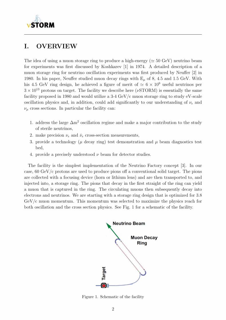
The facility is the simplest implementation of the Neutrino Factory concept [3]. In our

case, 60 GeV/c protons are used to produce pions off a conventional solid target. The pions

are collected with a focusing device (horn or lithium lens) and are then transported to, and

injected into, a storage ring. The pions that decay in the first straight of the ring can yield

a muon that is captured in the ring. The circulating muons then subsequently decay into

electrons and neutrinos. We are starting with a storage ring design that is optimized for 3.8

GeV/c muon momentum. This momentum was selected to maximize the physics reach for

both oscillation and the cross section physics. See Fig. 1 for a schematic of the facility.

Figure 1. Schematic of the facility

2

It would also be possible to create a π → µ decay channel and inject the muons into the

decay ring with a kicker magnet. This scheme would have the advantage that the transport

channel could be longer than the straight in the decay ring and thus allow for more π decays

to result in a useful µ. This does complicate the facility design, however, due to the need

for the kicker magnet and the desire to use single-turn extraction from the Main Injector.

Muon decay yields a neutrino beam of precisely known flavor content and energy. For

example for positive muons: µ+ → e+ + νµ + νe. In addition, if the circulating muon

flux in the ring is measured accurately (with beam-current transformers, for example), then

the neutrino beam flux is also accurately known. Near and far detectors are placed along

the line of one of the straight sections of the racetrack decay ring. The near detector can

be placed at 20-50 meters from the end of the straight. A near detector for disappearance

measurements will be identical to the far detector, but only about one tenth the fiducial

mass. It will require a µ catcher, however. Additional purpose-specific near detectors can

also be located in the near hall and will measure neutrino-nucleon cross sections. νSTORM

can provide the first precision measurements of νe and νe cross sections which are important

for future long-baseline experiments. A far detector at ≃ 2000 m would study neutrino

oscillation physics and would be capable of performing searches in both appearance and

disappearance channels. The experiment will take advantage of the “golden channel” of

oscillation appearance νe → νµ, where the resulting final state has a muon of the wrong-sign

from interactions of the νµ in the beam. In the case of µ+s stored in the ring, this would mean

the observation of an event with a µ−. This detector would need to be magnetized for the

wrong-sign muon appearance channel, as is the case for the current baseline Neutrino Factory

detector [4]. A number of possibilities for the far detector exist. However, a magnetized iron

detector similar to that used in MINOS is likely to be the most straight forward approach for

the far detector design. We believe that it will meet the performance requirements needed

to reach our physics goals. For the purposes of the νSTORM oscillation physics, a detector

inspired by MINOS, but with thinner plates and much larger excitation current (larger B

field) is assumed.

II. THEORETICAL AND EXPERIMENTAL MOTI-

VATIONS

A. Sterile neutrinos in extensions of the Standard Model

Sterile neutrinos, fermions that are uncharged under the SU(3)×SU(2)×U(1) gauge group,

arise naturally in many extensions to the Standard Model. Even where they are not an

integral part of a model, they can usually be easily accommodated. A detailed overview of

the phenomenology of sterile neutrinos and of related model building considerations is given

in [5].

For instance, in Grand Unified Theories (GUTs), fermions are grouped into multiplets of

3

a large gauge group, of which SU(3) × SU(2) × U(1) is a subgroup. If these multiplets

contain not only the known quarks and leptons, but also additional fermions, these new

fermions will, after the breaking of the GUT symmetry, often behave like gauge singlets (see

for instance [6–9] for GUT models with sterile neutrinos).

Models attempting to explain the smallness of neutrino masses through a seesaw mech-

anism generically contain sterile neutrinos. While in the most generic seesaw scenarios,

these sterile neutrinos are extremely heavy (∼ 1014 GeV) and have very small mixing angles

(∼ 10−12) with the active neutrinos, slightly non-minimal seesaw models can easily feature

sterile neutrinos with eV-scale masses and with percent level mixing with the active neutri-

nos. Examples for non-minimal seesaw models with relatively light sterile neutrinos include

the split seesaw scenario [10], seesaw models with additional flavor symmetries (see e.g. [11]),

models with a Froggatt-Nielsen mechanism [12, 13], and extended seesaw models that aug-

ment the mechanism by introducing more than three singlet fermions, as well as additional

symmetries [14–16].

Furthermore, sterile neutrinos arise naturally in “mirror models”, in which the existence

of an extended “dark sector”, with nontrivial dynamics of its own, is postulated. If the dark

sector is similar to the visible sector, as is the case, for instance, in string-inspired E8 × E8

models, it is natural to assume that it also contains neutrinos [17–19].

Finally, sterile neutrinos also have an impact in cosmology on the evolution of the Early

Universe and on astrophysical objects such as supernovae (for a review see [5] and references

therein). By mixing with active neutrinos, they can be produced in the Early Universe by

oscillations before neutrino decoupling. They could constitute the dark matter (DM) of

the Universe, if they have masses in the keV range, or part of it in the case of lighter

masses in the eV range, in which case they contribute to hot DM. A thermal population

of a light sterile neutrino acts as an additional relativistic degree of freedom at sufficiently

high temperatures. If present, they affect Big Bang Nucleosynthesis, the Cosmic Microwave

Background (CMB) and the formation of large scale structures such as galaxies and clusters

of galaxies. Their effect on the CMB anisotropies is due mainly to the change of the matter

radiation equality redshift and the sound horizon at the time of CMB decoupling and to their

anisotropic stress which suppresses the amplitude of higher harmonics in the temperature

anisotropy spectrum. Interestingly, recent observations of the CMB by WMAP and of the

CMB damping tail by ACT and SPT indicate a value of the effective number of relativistic

degrees of freedom higher than 3 at a significant confidence level, suggesting the existence

of sterile neutrinos or of a thermal population of other light particles, in addition to 3 active

neutrinos. If future observations, and in particular Planck, confirm this result, testing the

mixing angles required for a thermal distribution of sterile neutrinos to be produced in the

Early Universe will be of paramount importance in order to establish the identity of the

additional relativistic degrees of freedom in the Universe. νSTORM could test a large part

of the required parameter space, having sensitivity to the relevant masses and mixing angles

with different flavors.

4

B. Experimental hints for light sterile neutrinos

While the theoretical motivation for the existence of sterile neutrinos is certainly strong,

what has mostly prompted the interest of the scientific community in this topic are several

experimental results that show significant deviations from the Standard Model predictions.

These results can be interpreted as hints for oscillations involving sterile neutrinos.

The first of these hints was obtained by the LSND collaboration, who carried out a search

for νµ → νe oscillations over a baseline of ∼ 30 m [20]. Neutrinos were produced in a

stopped pion source in the decay π+ → µ+ + νµ and the subsequent decay µ+ → e+νµνe.

Electron antineutrinos are detected through the inverse beta decay reaction νep → e+n

in a liquid scintillator detector. Backgrounds to this search arise from the decay chain

π− → νµ + (µ− → νµνee−) if negative pions produced in the target decay before they are

captured by a nucleus, and from the reaction νµp → µ+n, which is only allowed for the small

fraction of muon antineutrinos produced by pion decay in flight rather than stopped pion

decay. The LSND collaboration finds an excess of νe candidate events above this background

with a significance of more than 3σ. When interpreted as νµ → νe oscillations through an

intermediate sterile state νs, this result is best explained by sterile neutrinos with an effective

mass squared splitting ∆m2 & 0.2 eV2 relative to the active neutrinos, and with an effective

sterile-induced νµ–νe mixing angle sin2 2θeµ,eff & 2× 10−3, depending on ∆m2.

The MiniBooNE experiment [21, 22] was designed to test the neutrino oscillation interpre-

tation of the LSND result using a different technique, namely neutrinos from a horn-focused

pion beam. While a MiniBooNE search for νµ → νe oscillations indeed disfavors most (but

not all) of the parameter region preferred by LSND in the simplest model with only one

sterile neutrino [21], the experiment obtains results consistent with LSND when running in

antineutrino mode and searching for νµ → νe. Due to low statistics, however, the antineu-

trino data favors LSND-like oscillations over the null hypothesis only at the 90% confidence

level. Moreover, MiniBooNE observes a yet unexplained 3.0σ excess of νe-like events (and,

with smaller significance also of νe events) at low energies, 200 MeV . Eν . 475 MeV,

outside the energy range where LSND-like oscillations would be expected.

A third hint for the possible existence of sterile neutrinos is provided by the so-called reac-

tor antineutrino anomaly. In 2011, Mueller et al. published a new ab initio computation of

the expected neutrino fluxes from nuclear reactors [23]. Their results improve upon a 1985

calculation by Schreckenbach [24] by using up-to-date nuclear databases, a careful treatment

of systematic uncertainties and various other corrections and improvements that were ne-

glected in the earlier calculation. Mueller et al. find that the predicted antineutrino flux

from a nuclear reactor is about 3% higher than previously thought. This result, which was

later confirmed by Huber [25], implies that short baseline reactor experiments have observed

a 3σ deficit of antineutrinos compared to the prediction [5, 26]. It needs to be emphasized

that the significance of the deficit depends crucially on the systematic uncertainties asso-

ciated with the theoretical prediction, some of which are difficult to estimate reliably. If

the reactor antineutrino deficit is interpreted as νe → νs disappearance via oscillation, the

required 2-flavor oscillation parameters are ∆m2 & 1 eV2 and sin2 2θee,eff ∼ 0.1.

5

Such short-baseline oscillations could also explain another experimental result: the Gallium

anomaly. The GALLEX and SAGE solar neutrino experiments used electron neutrinos

from intense artificial radioactive sources to test their radiochemical detection principle [27–

31]. Both experiments observed fewer νe from the source than expected. The statistical

significance of the deficit is above 99% and can be interpreted in terms of short-baseline

νe → νs disappearance with ∆m2 & 1 eV2 and sin2 2θee,eff ∼ 0.1–0.8. [32–34].

C. Constraints and global fit

While the previous section shows that there is an intriguing accumulation of hints for the

existence of new oscillation effects—possibly related to sterile neutrinos—in short-baseline

experiments, these hints are not undisputed. Several short-baseline oscillation experiments

did not confirm the observations from LSND, MiniBooNE, reactor experiments, and Gallium

experiments, and place very strong limits on the relevant regions of parameter space in sterile

neutrino models. To assess the viability of these models it is necessary to carry out a global

fit to all relevant experimental data sets, and several groups have endeavored to do so [5, 35–

39]. In Fig. 2 [5, 35], we show the current constraints on the parameter space of a 3 + 1

model (a model with three active neutrinos and one sterile neutrino). We have projected

the parameter space onto a plane spanned by the mass squared difference ∆m2 between the

heavy, mostly sterile mass eigenstate and the light, most active ones and by the effective

amplitude sin2 2θeµ,eff for νµ → νe 2-flavor oscillations to which LSND and MiniBooNE are

sensitive.

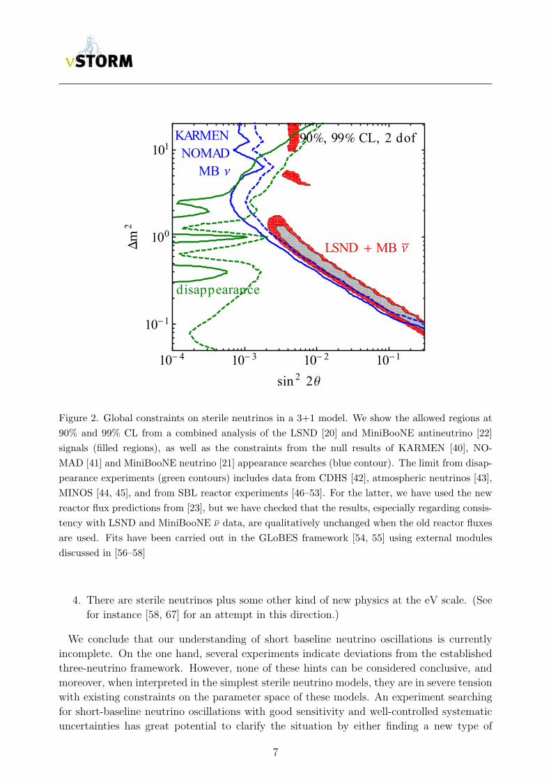
We see that there is severe tension in the global data set: the parameter region favored by

LSND and MiniBooNE antineutrino data is disfavored at more than 99% confidence level

by searches for νe (νe) and νµ disappearance. Using a parameter goodness-of-fit test [59] to

quantify this tension, p-values on the order of few× 10−6 are found for the compatibility of

LSND and MiniBooNe ν data with the rest of the global data set, and p-values smaller than

10−3 are found for the compatibility of appearance data and disappearance data [5]. The

global fit improves somewhat in models with more than one sterile neutrino, but significant

tension remains [5, 35].

One can imagine several possible resolutions to this puzzle:

1. One or several of the apparent deviations from the standard three neutrino oscillation

framework discussed in section II B have explanations not related to sterile neutrinos.

2. One or several of the null results that favor the no-oscillation hypothesis are in error.

3. There are more than two sterile neutrino flavors. Note that scenarios with one sterile

neutrino with an eV scale mass are already in some tension with cosmology, even

though the existence of one sterile neutrino with a mass well below 1 eV is actually

preferred by cosmological fits [60–63]. Cosmological bounds on sterile neutrinos can

be avoided in non-standard cosmologies [64] or by invoking mechanisms that suppress

sterile neutrino production in the early universe [65, 66].

6

10 4 10 3 10 2 101

101

100

101

sin 2 2Θ

m

2KARMENNOMAD

MB Ν

disappearance

LSND MB Ν

90, 99 CL, 2 dof

Figure 2. Global constraints on sterile neutrinos in a 3+1 model. We show the allowed regions at

90% and 99% CL from a combined analysis of the LSND [20] and MiniBooNE antineutrino [22]

signals (filled regions), as well as the constraints from the null results of KARMEN [40], NO-

MAD [41] and MiniBooNE neutrino [21] appearance searches (blue contour). The limit from disap-

pearance experiments (green contours) includes data from CDHS [42], atmospheric neutrinos [43],

MINOS [44, 45], and from SBL reactor experiments [46–53]. For the latter, we have used the new

reactor flux predictions from [23], but we have checked that the results, especially regarding consis-

tency with LSND and MiniBooNE ν data, are qualitatively unchanged when the old reactor fluxes

are used. Fits have been carried out in the GLoBES framework [54, 55] using external modules

discussed in [56–58]

4. There are sterile neutrinos plus some other kind of new physics at the eV scale. (See

for instance [58, 67] for an attempt in this direction.)

We conclude that our understanding of short baseline neutrino oscillations is currently

incomplete. On the one hand, several experiments indicate deviations from the established

three-neutrino framework. However, none of these hints can be considered conclusive, and

moreover, when interpreted in the simplest sterile neutrino models, they are in severe tension

with existing constraints on the parameter space of these models. An experiment searching

for short-baseline neutrino oscillations with good sensitivity and well-controlled systematic

uncertainties has great potential to clarify the situation by either finding a new type of

7

neutrino oscillation or by deriving a strong and robust constraint on any such oscillation.

The requirements for this proposed experiment are as follows:

• Direct test of the LSND and MiniBooNE anomalies.

• Provide stringent constraints for both νe and νµ disappearance to overconstrain 3+N

oscillation models and to test the Gallium and reactor anomalies directly.

• Test the CP- and T-conjugated channels as well, in order to obtain the relevant clues

for the underlying physics model, such as CP violation in 3 + 2 models.

Neutrino production with a muon storage ring is the only option which can fulfill these re-

quirements simultaneously, since both νe (νe) and νµ (νµ) are in the beam in equal quantities.

D. Measurement of neutrino-nucleon scattering cross sections

A number of recent articles have presented detailed reviews of the status of neutrino-nucleon

scattering cross section measurements in the context of the oscillation-physics program (see

for example [68] and references therein). The effect of uncertainties in the neutrino scattering

cross sections is to reduce the sensitivity of the present and future short- and long-baseline

experiments. The impact of the uncertainties on the cross sections is particularly pernicious

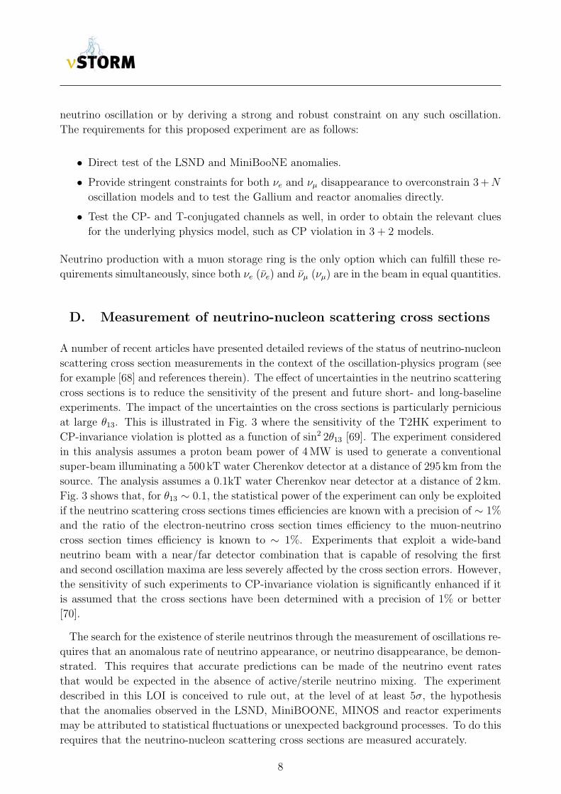
at large θ13. This is illustrated in Fig. 3 where the sensitivity of the T2HK experiment to

CP-invariance violation is plotted as a function of sin2 2θ13 [69]. The experiment considered

in this analysis assumes a proton beam power of 4MW is used to generate a conventional

super-beam illuminating a 500 kT water Cherenkov detector at a distance of 295 km from the

source. The analysis assumes a 0.1kT water Cherenkov near detector at a distance of 2 km.

Fig. 3 shows that, for θ13 ∼ 0.1, the statistical power of the experiment can only be exploited

if the neutrino scattering cross sections times efficiencies are known with a precision of ∼ 1%

and the ratio of the electron-neutrino cross section times efficiency to the muon-neutrino

cross section times efficiency is known to ∼ 1%. Experiments that exploit a wide-band

neutrino beam with a near/far detector combination that is capable of resolving the first

and second oscillation maxima are less severely affected by the cross section errors. However,

the sensitivity of such experiments to CP-invariance violation is significantly enhanced if it

is assumed that the cross sections have been determined with a precision of 1% or better

[70].

The search for the existence of sterile neutrinos through the measurement of oscillations re-

quires that an anomalous rate of neutrino appearance, or neutrino disappearance, be demon-

strated. This requires that accurate predictions can be made of the neutrino event rates

that would be expected in the absence of active/sterile neutrino mixing. The experiment

described in this LOI is conceived to rule out, at the level of at least 5σ, the hypothesis

that the anomalies observed in the LSND, MiniBOONE, MINOS and reactor experiments

may be attributed to statistical fluctuations or unexpected background processes. To do this

requires that the neutrino-nucleon scattering cross sections are measured accurately.

8

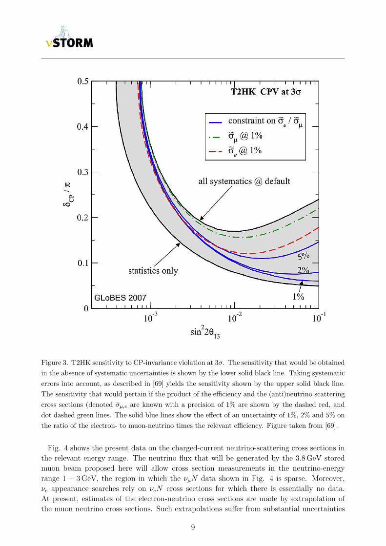
Figure 3. T2HK sensitivity to CP-invariance violation at 3σ. The sensitivity that would be obtained

in the absence of systematic uncertainties is shown by the lower solid black line. Taking systematic

errors into account, as described in [69] yields the sensitivity shown by the upper solid black line.

The sensitivity that would pertain if the product of the efficiency and the (anti)neutrino scattering

cross sections (denoted σµ,e are known with a precision of 1% are shown by the dashed red, and

dot dashed green lines. The solid blue lines show the effect of an uncertainty of 1%, 2% and 5% on

the ratio of the electron- to muon-neutrino times the relevant efficiency. Figure taken from [69].

Fig. 4 shows the present data on the charged-current neutrino-scattering cross sections in

the relevant energy range. The neutrino flux that will be generated by the 3.8GeV stored

muon beam proposed here will allow cross section measurements in the neutrino-energy

range 1 − 3GeV, the region in which the νµN data shown in Fig. 4 is sparse. Moreover,

νe appearance searches rely on νeN cross sections for which there is essentially no data.

At present, estimates of the electron-neutrino cross sections are made by extrapolation of

the muon neutrino cross sections. Such extrapolations suffer from substantial uncertainties

9

Figure 4. The neutrino-nucleon (left panel) and antineutrino-nucleon (right panel) cross sections

plotted as a function of (anti)neutrino energy [71]. The data are compared to the expectations of

the models described in [72]. The processes that contribute to the total cross section (shown by the

black lines) are: quasi-elastic (QE, red lines) scattering; resonance production (RES, blue lines);

and deep inelastic scattering (DIS, green lines). The uncertainties in the energy range of interest

are typically 10− 40%. Figure taken from [68].

arising from non-perturbative hadronic corrections and it is therefore essential that detailed

measurements of the νeN and νµN scattering cross sections and hadron-production rates

are performed. The νSTORM facility, therefore, has a unique opportunity. The flavor

composition of the beam and the neutrino energy spectrum are both known precisely. In

addition, the storage ring instrumentation combined with measurements at the near detector

will allow the neutrino flux to be measured with a precision of 1%. Substantial event rates

may be obtained in a fine-grained detector placed between 20m and 50m from the storage

ring. Therefore, the objective is to measure the νeN and νµN scattering cross sections for

neutrino energies in the range 1 − 3GeV with a precision approaching 1%. This will be a

critical contribution to the search for sterile neutrinos and will be of fundamental importance

to the present and next generation of long-baseline neutrino oscillation experiments.

III. FACILITY

The basic concept for the facility is presented in Fig. 1. A high-intensity proton source places

beam on a target, producing a large spectrum of secondary pions. Forward pions are focused

by a collection element into a transport channel. Pions decay within the first straight of the

decay ring and a fraction of the resulting muons are stored in the ring. Muon decay within

the straight sections will produce ν beams of known flux and flavor via: µ+ → e+ + νµ +

νe or µ− → e− + νµ + νe. For the implementation which is described here, we choose a 3.8

GeV/c storage ring to obtain the desired spectrum of ≃ 2 GeV neutrinos (see Fig. 42). This

means that we must capture pions at a momentum of approximately 5 GeV/c.

10

momentum (GeV/c)

π+/POT

70 cm Be32.2 cm C(diamond)

21 cm Au

27 cm inconel21.3 cm Ta

momentum (GeV/c)

π-/POT

0.0020.0040.0060.0080.01

0.0120.0140.0160.0180.02

2 3 4 5 6 7 8 9 10

0.0020.0040.0060.0080.01

0.0120.0140.0160.0180.02

2 3 4 5 6 7 8 9 10

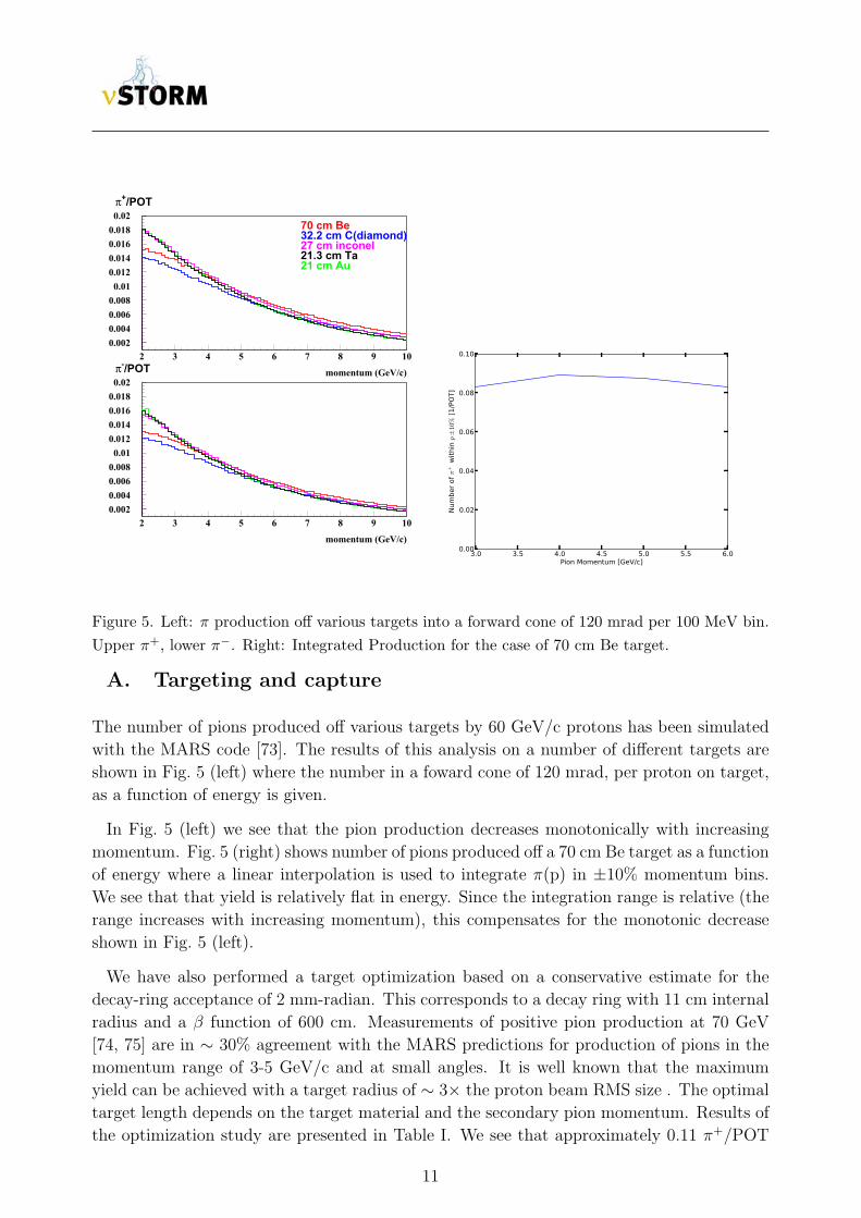
Figure 5. Left: π production off various targets into a forward cone of 120 mrad per 100 MeV bin.

Upper π+, lower π−. Right: Integrated Production for the case of 70 cm Be target.

A. Targeting and capture

The number of pions produced off various targets by 60 GeV/c protons has been simulated

with the MARS code [73]. The results of this analysis on a number of different targets are

shown in Fig. 5 (left) where the number in a foward cone of 120 mrad, per proton on target,

as a function of energy is given.

In Fig. 5 (left) we see that the pion production decreases monotonically with increasing

momentum. Fig. 5 (right) shows number of pions produced off a 70 cm Be target as a function

of energy where a linear interpolation is used to integrate π(p) in ±10% momentum bins.

We see that that yield is relatively flat in energy. Since the integration range is relative (the

range increases with increasing momentum), this compensates for the monotonic decrease

shown in Fig. 5 (left).

We have also performed a target optimization based on a conservative estimate for the

decay-ring acceptance of 2 mm-radian. This corresponds to a decay ring with 11 cm internal

radius and a β function of 600 cm. Measurements of positive pion production at 70 GeV

[74, 75] are in ∼ 30% agreement with the MARS predictions for production of pions in the

momentum range of 3-5 GeV/c and at small angles. It is well known that the maximum

yield can be achieved with a target radius of ∼ 3× the proton beam RMS size . The optimal

target length depends on the target material and the secondary pion momentum. Results of

the optimization study are presented in Table I. We see that approximately 0.11 π+/POT

11

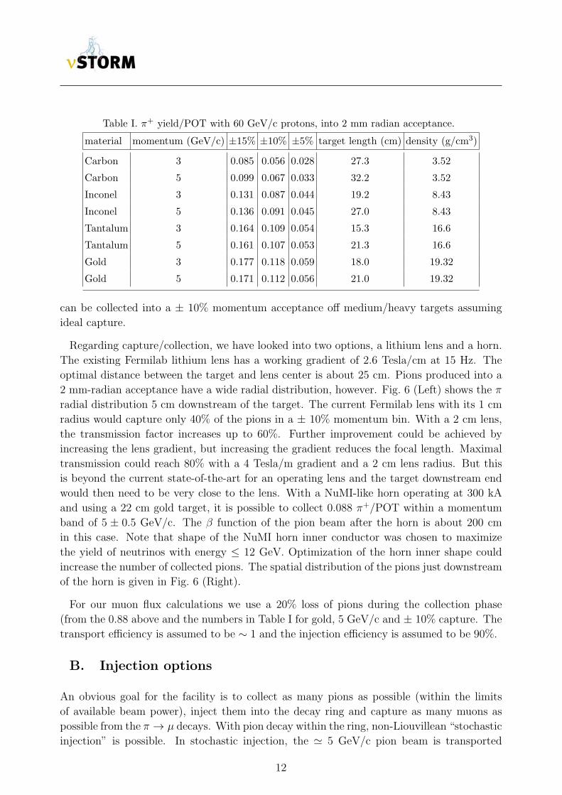
Table I. π+ yield/POT with 60 GeV/c protons, into 2 mm radian acceptance.

material momentum (GeV/c) ±15% ±10% ±5% target length (cm) density (g/cm3)

Carbon 3 0.085 0.056 0.028 27.3 3.52

Carbon 5 0.099 0.067 0.033 32.2 3.52

Inconel 3 0.131 0.087 0.044 19.2 8.43

Inconel 5 0.136 0.091 0.045 27.0 8.43

Tantalum 3 0.164 0.109 0.054 15.3 16.6

Tantalum 5 0.161 0.107 0.053 21.3 16.6

Gold 3 0.177 0.118 0.059 18.0 19.32

Gold 5 0.171 0.112 0.056 21.0 19.32

can be collected into a ± 10% momentum acceptance off medium/heavy targets assuming

ideal capture.

Regarding capture/collection, we have looked into two options, a lithium lens and a horn.

The existing Fermilab lithium lens has a working gradient of 2.6 Tesla/cm at 15 Hz. The

optimal distance between the target and lens center is about 25 cm. Pions produced into a

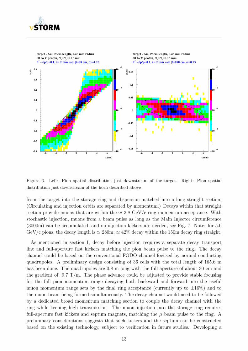
2 mm-radian acceptance have a wide radial distribution, however. Fig. 6 (Left) shows the π

radial distribution 5 cm downstream of the target. The current Fermilab lens with its 1 cm

radius would capture only 40% of the pions in a ± 10% momentum bin. With a 2 cm lens,

the transmission factor increases up to 60%. Further improvement could be achieved by

increasing the lens gradient, but increasing the gradient reduces the focal length. Maximal

transmission could reach 80% with a 4 Tesla/m gradient and a 2 cm lens radius. But this

is beyond the current state-of-the-art for an operating lens and the target downstream end

would then need to be very close to the lens. With a NuMI-like horn operating at 300 kA

and using a 22 cm gold target, it is possible to collect 0.088 π+/POT within a momentum

band of 5 ± 0.5 GeV/c. The β function of the pion beam after the horn is about 200 cm

in this case. Note that shape of the NuMI horn inner conductor was chosen to maximize

the yield of neutrinos with energy ≤ 12 GeV. Optimization of the horn inner shape could

increase the number of collected pions. The spatial distribution of the pions just downstream

of the horn is given in Fig. 6 (Right).

For our muon flux calculations we use a 20% loss of pions during the collection phase

(from the 0.88 above and the numbers in Table I for gold, 5 GeV/c and ± 10% capture. The

transport efficiency is assumed to be ∼ 1 and the injection efficiency is assumed to be 90%.

B. Injection options

An obvious goal for the facility is to collect as many pions as possible (within the limits

of available beam power), inject them into the decay ring and capture as many muons as

possible from the π → µ decays. With pion decay within the ring, non-Liouvillean “stochastic

injection” is possible. In stochastic injection, the ≃ 5 GeV/c pion beam is transported

12

10-6

10-5

10-4

10-3

10-2

x (cm)

dx/d

s

target - Au, 19 cm length, 0.45 mm radius60 GeV proton, σx=σy=0.15 mmπ+ - δp/p=0.1, ε= 2 mm rad, β=88 cm, α=-4.25

-0.4

-0.3

-0.2

-0.1

0

0.1

0.2

0.3

0.4

-6 -4 -2 0 2 4 610

-6

10-5

10-4

10-3

10-2

x (cm)

dx/d

s

target - Au, 19 cm length, 0.45 mm radius60 GeV proton, σx=σy=0.15 mmπ+ - δp/p=0.1, ε= 2 mm rad, β=180 cm, α=0.75

-0.15

-0.1

-0.05

0

0.05

0.1

0.15

-6 -4 -2 0 2 4 6

Figure 6. Left: Pion spatial distribution just downstream of the target. Right: Pion spatial

distribution just downstream of the horn described above

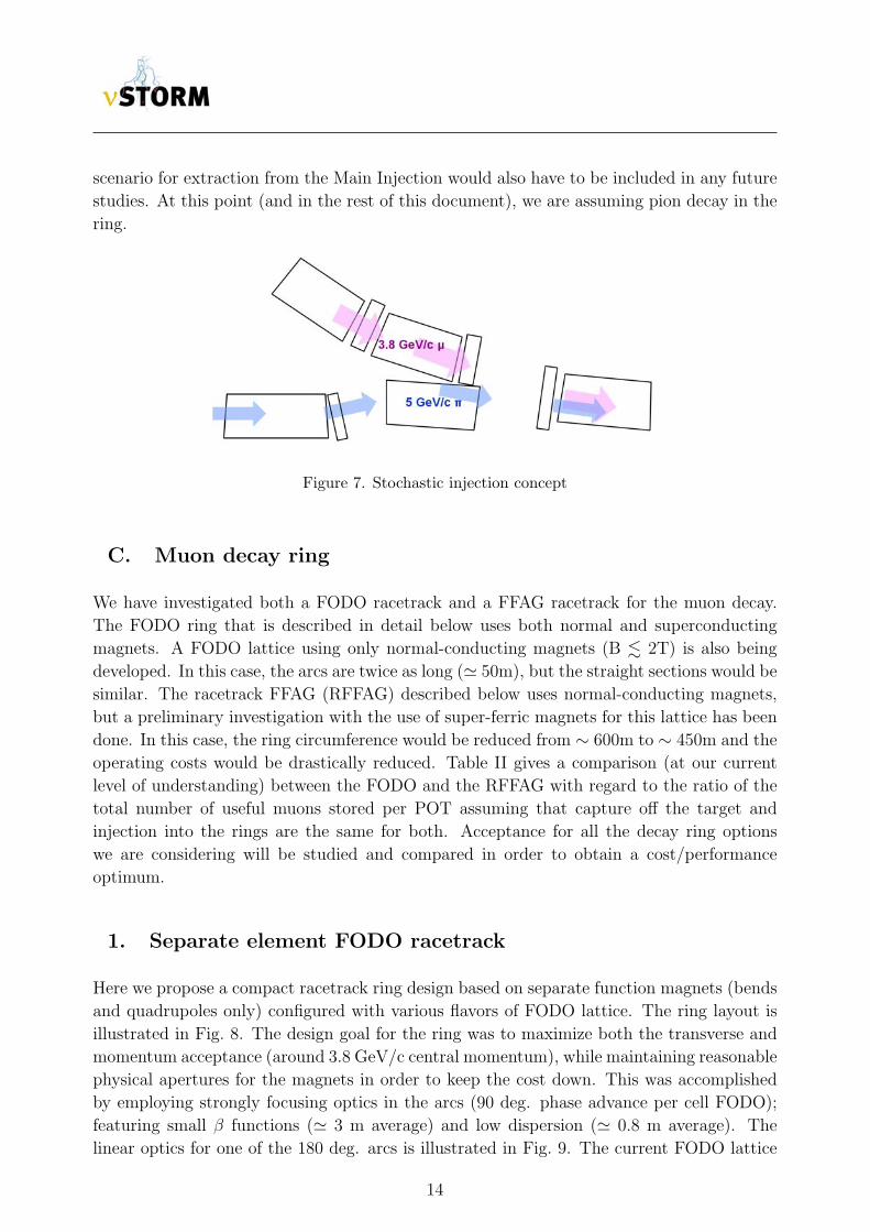
from the target into the storage ring and dispersion-matched into a long straight section.

(Circulating and injection orbits are separated by momentum.) Decays within that straight

section provide muons that are within the 3.8 GeV/c ring momentum acceptance. With

stochastic injection, muons from a beam pulse as long as the Main Injector circumference

(3000m) can be accumulated, and no injection kickers are needed, see Fig. 7. Note: for 5.0

GeV/c pions, the decay length is 280m; 42% decay within the 150m decay ring straight.

As mentioned in section I, decay before injection requires a separate decay transport

line and full-aperture fast kickers matching the pion beam pulse to the ring. The decay

channel could be based on the conventional FODO channel focused by normal conducting

quadrupoles. A preliminary design consisting of 36 cells with the total length of 165.6 m

has been done. The quadrupoles are 0.8 m long with the full aperture of about 30 cm and

the gradient of 9.7 T/m. The phase advance could be adjusted to provide stable focusing

for the full pion momentum range decaying both backward and forward into the useful

muon momentum range sets by the final ring acceptance (currently up to ±16%) and to

the muon beam being formed simultaneously. The decay channel would need to be followed

by a dedicated broad momentum matching section to couple the decay channel with the

ring while keeping high transmission. The muon injection into the storage ring requires

full-aperture fast kickers and septum magnets, matching the µ beam pulse to the ring. A

preliminary considerations suggests that such kickers and the septum can be constructed

based on the existing technology, subject to verification in future studies. Developing a

13

scenario for extraction from the Main Injection would also have to be included in any future

studies. At this point (and in the rest of this document), we are assuming pion decay in the

ring.

Figure 7. Stochastic injection concept

C. Muon decay ring

We have investigated both a FODO racetrack and a FFAG racetrack for the muon decay.

The FODO ring that is described in detail below uses both normal and superconducting

magnets. A FODO lattice using only normal-conducting magnets (B 2T) is also being

developed. In this case, the arcs are twice as long ( 50m), but the straight sections would be

similar. The racetrack FFAG (RFFAG) described below uses normal-conducting magnets,

but a preliminary investigation with the use of super-ferric magnets for this lattice has been

done. In this case, the ring circumference would be reduced from ∼ 600m to ∼ 450m and the

operating costs would be drastically reduced. Table II gives a comparison (at our current

level of understanding) between the FODO and the RFFAG with regard to the ratio of the

total number of useful muons stored per POT assuming that capture off the target and

injection into the rings are the same for both. Acceptance for all the decay ring options

we are considering will be studied and compared in order to obtain a cost/performance

optimum.

1. Separate element FODO racetrack

Here we propose a compact racetrack ring design based on separate function magnets (bends

and quadrupoles only) configured with various flavors of FODO lattice. The ring layout is

illustrated in Fig. 8. The design goal for the ring was to maximize both the transverse and

momentum acceptance (around 3.8 GeV/c central momentum), while maintaining reasonable

physical apertures for the magnets in order to keep the cost down. This was accomplished

by employing strongly focusing optics in the arcs (90 deg. phase advance per cell FODO);

featuring small β functions ( 3 m average) and low dispersion ( 0.8 m average). The

linear optics for one of the 180 deg. arcs is illustrated in Fig. 9. The current FODO lattice

14

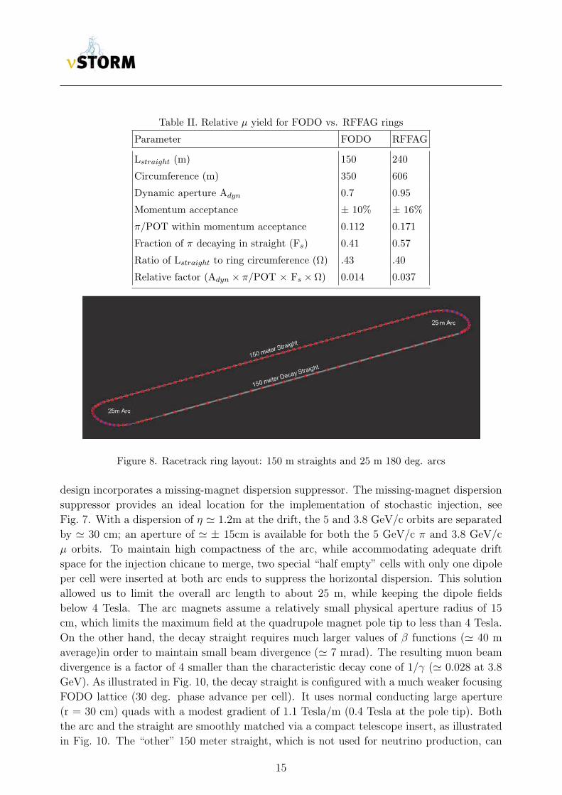
Table II. Relative µ yield for FODO vs. RFFAG rings

Parameter FODO RFFAG

Lstraight (m) 150 240

Circumference (m) 350 606

Dynamic aperture Adyn 0.7 0.95

Momentum acceptance ± 10% ± 16%

π/POT within momentum acceptance 0.112 0.171

Fraction of π decaying in straight (Fs) 0.41 0.57

Ratio of Lstraight to ring circumference (Ω) .43 .40

Relative factor (Adyn × π/POT × Fs × Ω) 0.014 0.037

Figure 8. Racetrack ring layout: 150 m straights and 25 m 180 deg. arcs

design incorporates a missing-magnet dispersion suppressor. The missing-magnet dispersion

suppressor provides an ideal location for the implementation of stochastic injection, see

Fig. 7. With a dispersion of η 1.2m at the drift, the 5 and 3.8 GeV/c orbits are separated

by 30 cm; an aperture of ± 15cm is available for both the 5 GeV/c π and 3.8 GeV/c

µ orbits. To maintain high compactness of the arc, while accommodating adequate drift

space for the injection chicane to merge, two special “half empty” cells with only one dipole

per cell were inserted at both arc ends to suppress the horizontal dispersion. This solution

allowed us to limit the overall arc length to about 25 m, while keeping the dipole fields

below 4 Tesla. The arc magnets assume a relatively small physical aperture radius of 15

cm, which limits the maximum field at the quadrupole magnet pole tip to less than 4 Tesla.

On the other hand, the decay straight requires much larger values of β functions ( 40 m

average)in order to maintain small beam divergence ( 7 mrad). The resulting muon beam

divergence is a factor of 4 smaller than the characteristic decay cone of 1/γ ( 0.028 at 3.8

GeV). As illustrated in Fig. 10, the decay straight is configured with a much weaker focusing

FODO lattice (30 deg. phase advance per cell). It uses normal conducting large aperture

(r = 30 cm) quads with a modest gradient of 1.1 Tesla/m (0.4 Tesla at the pole tip). Both

the arc and the straight are smoothly matched via a compact telescope insert, as illustrated

in Fig. 10. The “other” 150 meter straight, which is not used for neutrino production, can

15

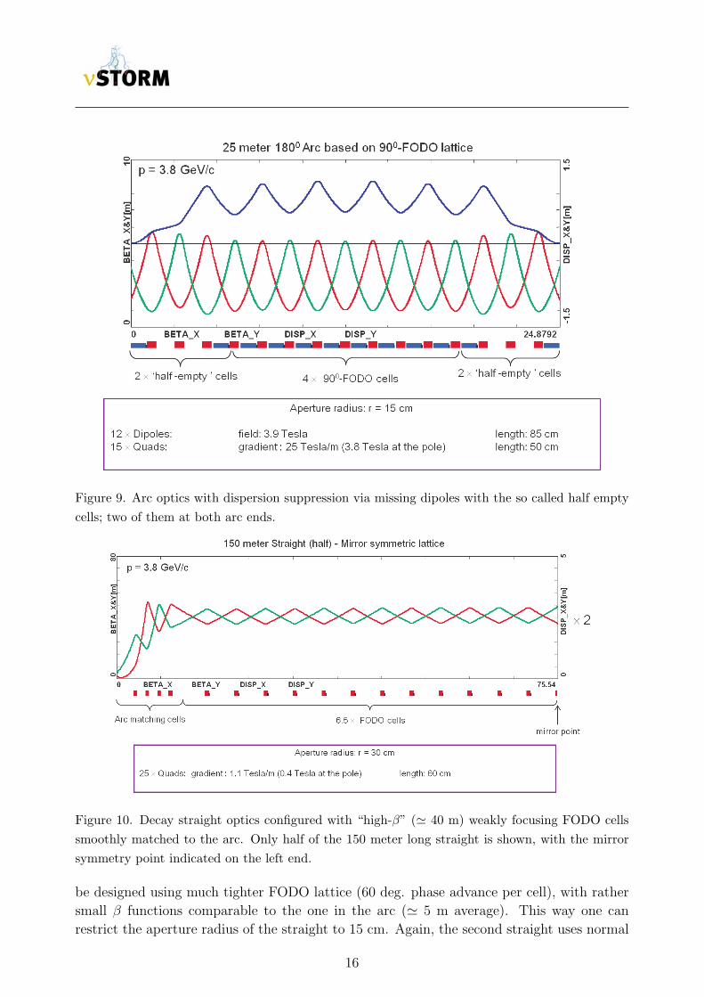
Figure 9. Arc optics with dispersion suppression via missing dipoles with the so called half empty

cells; two of them at both arc ends.

Figure 10. Decay straight optics configured with “high-β” ( 40 m) weakly focusing FODO cells

smoothly matched to the arc. Only half of the 150 meter long straight is shown, with the mirror

symmetry point indicated on the left end.

be designed using much tighter FODO lattice (60 deg. phase advance per cell), with rather

small β functions comparable to the one in the arc ( 5 m average). This way one can

restrict the aperture radius of the straight to 15 cm. Again, the second straight uses normal

16

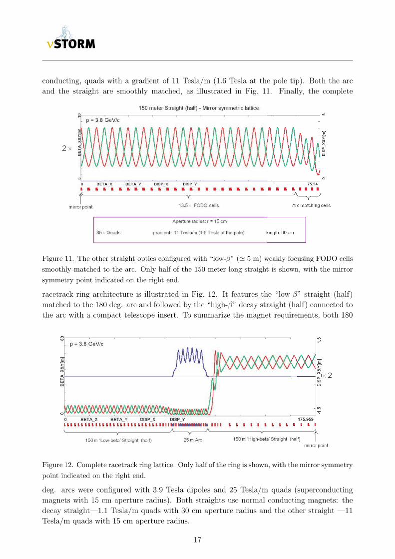
conducting, quads with a gradient of 11 Tesla/m (1.6 Tesla at the pole tip). Both the arc

and the straight are smoothly matched, as illustrated in Fig. 11. Finally, the complete

Figure 11. The other straight optics configured with “low-β” ( 5 m) weakly focusing FODO cells

smoothly matched to the arc. Only half of the 150 meter long straight is shown, with the mirror

symmetry point indicated on the right end.

racetrack ring architecture is illustrated in Fig. 12. It features the “low-β” straight (half)

matched to the 180 deg. arc and followed by the “high-β” decay straight (half) connected to

the arc with a compact telescope insert. To summarize the magnet requirements, both 180

Figure 12. Complete racetrack ring lattice. Only half of the ring is shown, with the mirror symmetry

point indicated on the right end.

deg. arcs were configured with 3.9 Tesla dipoles and 25 Tesla/m quads (superconducting

magnets with 15 cm aperture radius). Both straights use normal conducting magnets: the

decay straight—1.1 Tesla/m quads with 30 cm aperture radius and the other straight —11

Tesla/m quads with 15 cm aperture radius.

17

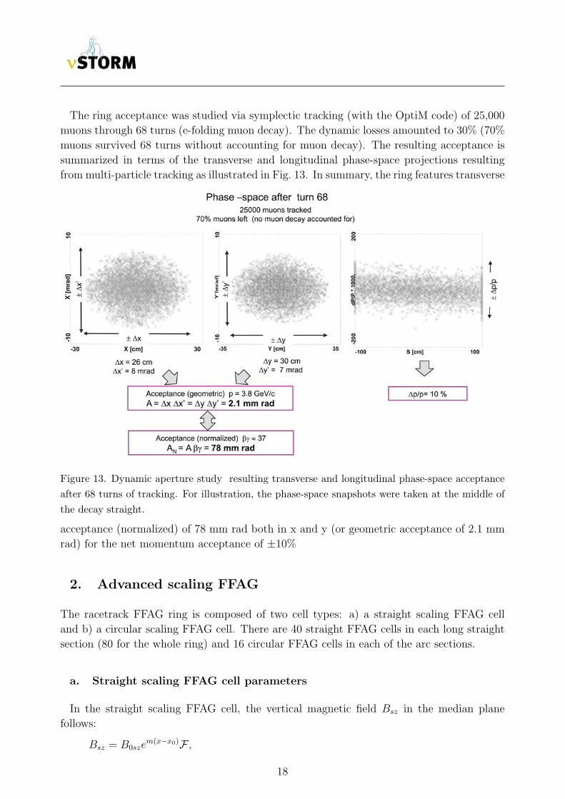
The ring acceptance was studied via symplectic tracking (with the OptiM code) of 25,000

muons through 68 turns (e-folding muon decay). The dynamic losses amounted to 30% (70%

muons survived 68 turns without accounting for muon decay). The resulting acceptance is

summarized in terms of the transverse and longitudinal phase-space projections resulting

from multi-particle tracking as illustrated in Fig. 13. In summary, the ring features transverse

Figure 13. Dynamic aperture study resulting transverse and longitudinal phase-space acceptance

after 68 turns of tracking. For illustration, the phase-space snapshots were taken at the middle of

the decay straight.

acceptance (normalized) of 78 mm rad both in x and y (or geometric acceptance of 2.1 mm

rad) for the net momentum acceptance of ±10%

2. Advanced scaling FFAG

The racetrack FFAG ring is composed of two cell types: a) a straight scaling FFAG cell

and b) a circular scaling FFAG cell. There are 40 straight FFAG cells in each long straight

section (80 for the whole ring) and 16 circular FFAG cells in each of the arc sections.

a. Straight scaling FFAG cell parameters

In the straight scaling FFAG cell, the vertical magnetic field Bsz in the median plane

follows:

Bsz = B0szem(x−x0)F ,

18

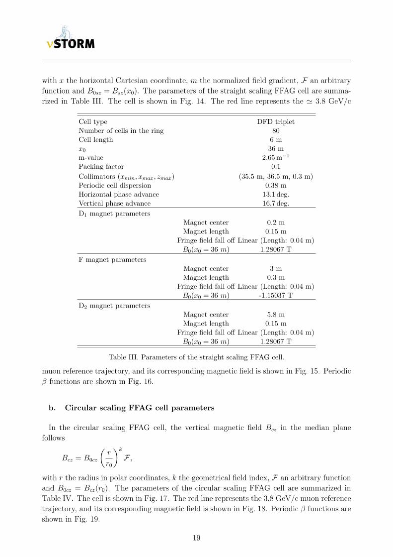
with x the horizontal Cartesian coordinate, m the normalized field gradient, F an arbitrary

function and B0sz = Bsz(x0). The parameters of the straight scaling FFAG cell are summa-

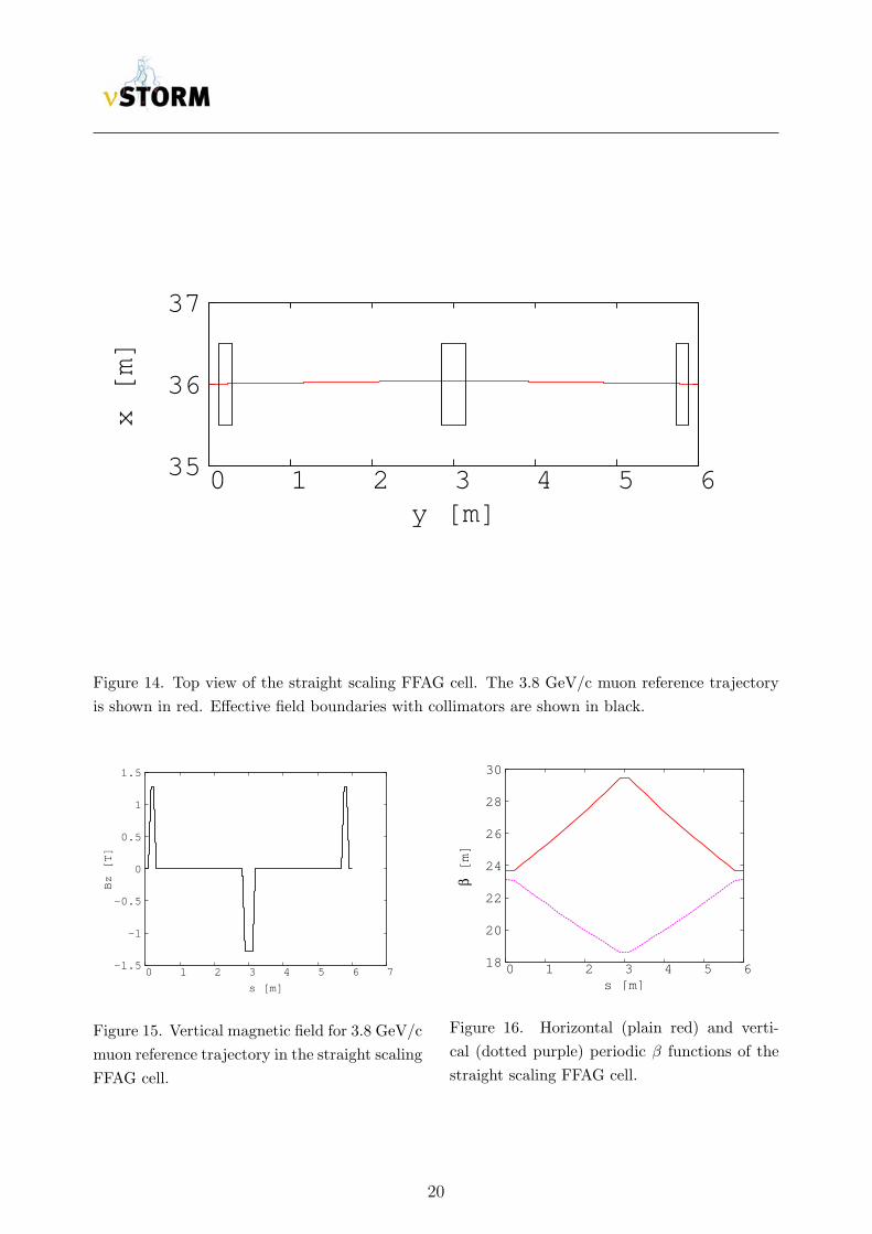
rized in Table III. The cell is shown in Fig. 14. The red line represents the ≃ 3.8 GeV/c

Cell type DFD tripletNumber of cells in the ring 80Cell length 6 mx0 36 mm-value 2.65m−1

Packing factor 0.1

Collimators (xmin, xmax, zmax) (35.5 m, 36.5 m, 0.3 m)Periodic cell dispersion 0.38 mHorizontal phase advance 13.1 deg.Vertical phase advance 16.7 deg.

D1 magnet parametersMagnet center 0.2 mMagnet length 0.15 m

Fringe field fall off Linear (Length: 0.04 m)B0(x0 = 36 m) 1.28067 T

F magnet parametersMagnet center 3 mMagnet length 0.3 m

Fringe field fall off Linear (Length: 0.04 m)B0(x0 = 36 m) -1.15037 T

D2 magnet parametersMagnet center 5.8 mMagnet length 0.15 m

Fringe field fall off Linear (Length: 0.04 m)B0(x0 = 36 m) 1.28067 T

Table III. Parameters of the straight scaling FFAG cell.

muon reference trajectory, and its corresponding magnetic field is shown in Fig. 15. Periodic

β functions are shown in Fig. 16.

b. Circular scaling FFAG cell parameters

In the circular scaling FFAG cell, the vertical magnetic field Bcz in the median plane

follows

Bcz = B0cz

(r

r0

)k

F ,

with r the radius in polar coordinates, k the geometrical field index, F an arbitrary function

and B0cz = Bcz(r0). The parameters of the circular scaling FFAG cell are summarized in

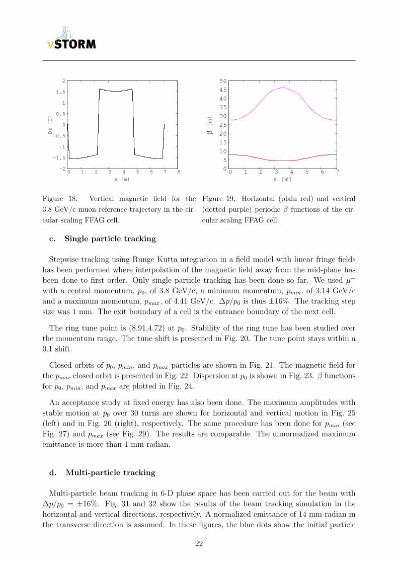
Table IV. The cell is shown in Fig. 17. The red line represents the 3.8 GeV/c muon reference

trajectory, and its corresponding magnetic field is shown in Fig. 18. Periodic β functions are

shown in Fig. 19.

19

35

36

37

0 1 2 3 4 5 6

x [m]

y [m]

Figure 14. Top view of the straight scaling FFAG cell. The 3.8 GeV/c muon reference trajectory

is shown in red. Effective field boundaries with collimators are shown in black.

-1.5

-1

-0.5

0

0.5

1

1.5

0 1 2 3 4 5 6 7

Bz [T]

s [m]

Figure 15. Vertical magnetic field for 3.8 GeV/c

muon reference trajectory in the straight scaling

FFAG cell.

18

20

22

24

26

28

30

0 1 2 3 4 5 6

β [m]

s [m]

Figure 16. Horizontal (plain red) and verti-

cal (dotted purple) periodic β functions of the

straight scaling FFAG cell.

20

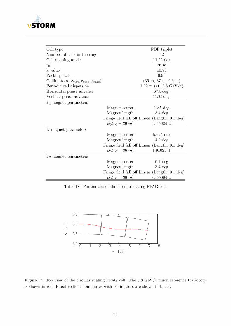
Cell type FDF tripletNumber of cells in the ring 32Cell opening angle 11.25 degr0 36 mk-value 10.85Packing factor 0.96Collimators (rmin, rmax, zmax) (35 m, 37 m, 0.3 m)Periodic cell dispersion 1.39 m (at 3.8 GeV/c)Horizontal phase advance 67.5 deg.Vertical phase advance 11.25 deg.

F1 magnet parametersMagnet center 1.85 degMagnet length 3.4 deg

Fringe field fall off Linear (Length: 0.1 deg)B0(r0 = 36 m) -1.55684 T

D magnet parametersMagnet center 5.625 degMagnet length 4.0 deg

Fringe field fall off Linear (Length: 0.1 deg)B0(r0 = 36 m) 1.91025 T

F2 magnet parametersMagnet center 9.4 degMagnet length 3.4 deg

Fringe field fall off Linear (Length: 0.1 deg)B0(r0 = 36 m) -1.55684 T

Table IV. Parameters of the circular scaling FFAG cell.

34

35

36

37

0 1 2 3 4 5 6 7 8

x [m]

y [m]

Figure 17. Top view of the circular scaling FFAG cell. The 3.8 GeV/c muon reference trajectory

is shown in red. Effective field boundaries with collimators are shown in black.

21

-2

-1.5

-1

-0.5

0

0.5

1

1.5

2

0 1 2 3 4 5 6 7 8

Bz [T]

s [m]

Figure 18. Vertical magnetic field for the

3.8 GeV/c muon reference trajectory in the cir-

cular scaling FFAG cell.

0

5

10

15

20

25

30

35

40

45

50

0 1 2 3 4 5 6 7

β [m]

s [m]

Figure 19. Horizontal (plain red) and vertical

(dotted purple) periodic β functions of the cir-

cular scaling FFAG cell.

c. Single particle tracking

Stepwise tracking using Runge Kutta integration in a field model with linear fringe fields

has been performed where interpolation of the magnetic field away from the mid-plane has

been done to first order. Only single particle tracking has been done so far. We used µ+

with a central momentum, p0, of 3.8 GeV/c, a minimum momentum, pmin, of 3.14 GeV/c

and a maximum momentum, pmax, of 4.41 GeV/c. ∆p/p0 is thus ±16%. The tracking step

size was 1 mm. The exit boundary of a cell is the entrance boundary of the next cell.

The ring tune point is (8.91,4.72) at p0. Stability of the ring tune has been studied over

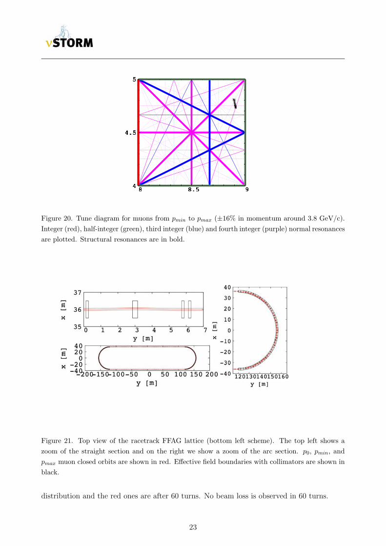
the momentum range. The tune shift is presented in Fig. 20. The tune point stays within a

0.1 shift.

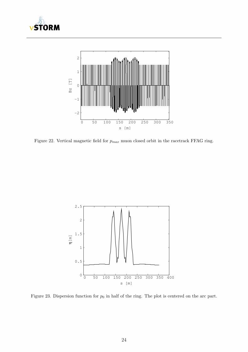
Closed orbits of p0, pmin, and pmax particles are shown in Fig. 21. The magnetic field for

the pmax closed orbit is presented in Fig. 22. Dispersion at p0 is shown in Fig. 23. β functions

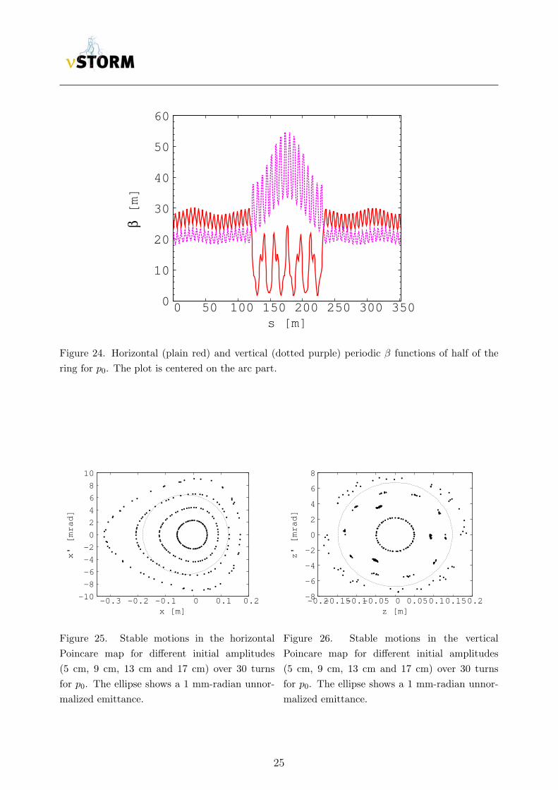
for p0, pmin, and pmax are plotted in Fig. 24.

An acceptance study at fixed energy has also been done. The maximum amplitudes with

stable motion at p0 over 30 turns are shown for horizontal and vertical motion in Fig. 25

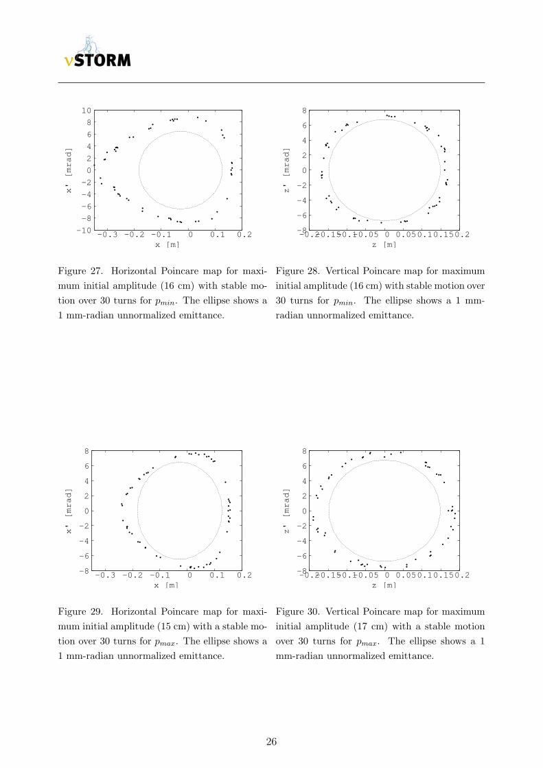
(left) and in Fig. 26 (right), respectively. The same procedure has been done for pmin (see

Fig. 27) and pmax (see Fig. 29). The results are comparable. The unnormalized maximum

emittance is more than 1 mm-radian.

d. Multi-particle tracking

Multi-particle beam tracking in 6-D phase space has been carried out for the beam with

∆p/p0 = ±16%. Fig. 31 and 32 show the results of the beam tracking simulation in the

horizontal and vertical directions, respectively. A normalized emittance of 14 mm-radian in

the transverse direction is assumed. In these figures, the blue dots show the initial particle

22

4

4.5

5

8 8.5 9 4

4.5

5

8 8.5 9 4

4.5

5

8 8.5 9 4

4.5

5

8 8.5 9 4

4.5

5

8 8.5 9 4

4.5

5

8 8.5 9 4

4.5

5

8 8.5 9 4

4.5

5

8 8.5 9 4

4.5

5

8 8.5 9 4

4.5

5

8 8.5 9 4

4.5

5

8 8.5 9

Figure 20. Tune diagram for muons from pmin to pmax (±16% in momentum around 3.8 GeV/c).

Integer (red), half-integer (green), third integer (blue) and fourth integer (purple) normal resonances

are plotted. Structural resonances are in bold.

Figure 21. Top view of the racetrack FFAG lattice (bottom left scheme). The top left shows a

zoom of the straight section and on the right we show a zoom of the arc section. p0, pmin, and

pmax muon closed orbits are shown in red. Effective field boundaries with collimators are shown in

black.

distribution and the red ones are after 60 turns. No beam loss is observed in 60 turns.

23

-2

-1

0

1

2

0 50 100 150 200 250 300 350

Bz [T]

s [m]

Figure 22. Vertical magnetic field for pmax muon closed orbit in the racetrack FFAG ring.

0

0.5

1

1.5

2

2.5

0 50 100 150 200 250 300 350 400

η[

m]

s [m]

Figure 23. Dispersion function for p0 in half of the ring. The plot is centered on the arc part.

24

0

10

20

30

40

50

60

0 50 100 150 200 250 300 350

β [m]

s [m]

Figure 24. Horizontal (plain red) and vertical (dotted purple) periodic β functions of half of the

ring for p0. The plot is centered on the arc part.

-10

-8

-6

-4

-2

0

2

4

6

8

10

-0.3 -0.2 -0.1 0 0.1 0.2

x' [mrad]

x [m]

Figure 25. Stable motions in the horizontal

Poincare map for different initial amplitudes

(5 cm, 9 cm, 13 cm and 17 cm) over 30 turns

for p0. The ellipse shows a 1 mm-radian unnor-

malized emittance.

-8

-6

-4

-2

0

2

4

6

8

-0.2-0.15-0.1-0.05 0 0.05 0.1 0.15 0.2

z' [mrad]

z [m]

Figure 26. Stable motions in the vertical

Poincare map for different initial amplitudes

(5 cm, 9 cm, 13 cm and 17 cm) over 30 turns

for p0. The ellipse shows a 1 mm-radian unnor-

malized emittance.

25

-10

-8

-6

-4

-2

0

2

4

6

8

10

-0.3 -0.2 -0.1 0 0.1 0.2

x' [mrad]

x [m]

Figure 27. Horizontal Poincare map for maxi-

mum initial amplitude (16 cm) with stable mo-

tion over 30 turns for pmin. The ellipse shows a

1 mm-radian unnormalized emittance.

-8

-6

-4

-2

0

2

4

6

8

-0.2-0.15-0.1-0.05 0 0.05 0.1 0.15 0.2

z' [mrad]

z [m]

Figure 28. Vertical Poincare map for maximum

initial amplitude (16 cm) with stable motion over

30 turns for pmin. The ellipse shows a 1 mm-

radian unnormalized emittance.

-8

-6

-4

-2

0

2

4

6

8

-0.3 -0.2 -0.1 0 0.1 0.2

x' [mrad]

x [m]

Figure 29. Horizontal Poincare map for maxi-

mum initial amplitude (15 cm) with a stable mo-

tion over 30 turns for pmax. The ellipse shows a

1 mm-radian unnormalized emittance.

-8

-6

-4

-2

0

2

4

6

8

-0.2-0.15-0.1-0.05 0 0.05 0.1 0.15 0.2

z' [mrad]

z [m]

Figure 30. Vertical Poincare map for maximum

initial amplitude (17 cm) with a stable motion

over 30 turns for pmax. The ellipse shows a 1

mm-radian unnormalized emittance.

26

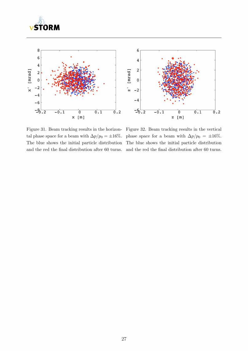
Figure 31. Beam tracking results in the horizon-

tal phase space for a beam with ∆p/p0 = ±16%.

The blue shows the initial particle distribution

and the red the final distribution after 60 turns.

Figure 32. Beam tracking results in the vertical

phase space for a beam with ∆p/p0 = ±16%.

The blue shows the initial particle distribution

and the red the final distribution after 60 turns.

27

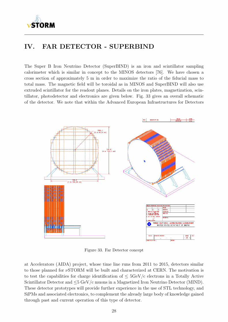
IV. FAR DETECTOR - SUPERBIND

The Super B Iron Neutrino Detector (SuperBIND) is an iron and scintillator sampling

calorimeter which is similar in concept to the MINOS detectors [76]. We have chosen a

cross section of approximately 5 m in order to maximize the ratio of the fiducial mass to

total mass. The magnetic field will be toroidal as in MINOS and SuperBIND will also use

extruded scintillator for the readout planes. Details on the iron plates, magnetization, scin-

tillator, photodetector and electronics are given below. Fig. 33 gives an overall schematic

of the detector. We note that within the Advanced European Infrastructures for Detectors

Figure 33. Far Detector concept

at Accelerators (AIDA) project, whose time line runs from 2011 to 2015, detectors similar

to those planned for νSTORM will be built and characterized at CERN. The motivation is

to test the capabilities for charge identification of ≤ 5GeV/c electrons in a Totally Active

Scintillator Detector and ≤5 GeV/c muons in a Magnetized Iron Neutrino Detector (MIND).

These detector prototypes will provide further experience in the use of STL technology, and

SiPMs and associated electronics, to complement the already large body of knowledge gained

through past and current operation of this type of detector.

28

A. Iron Plates

For the Iron plates in SuperBIND, we are pursuing the following design strategy. The

plates are cylinders with an overall diameter of 5 m and and depth of 1-2 cm. Our original

engineering design uses 1 cm plates, but we have simulated the detector performance for

both 1 cm and 2 cm thick plates. They are fabricated from two semicircles that are skip

welded together. Instead of hanging the plates on ears (as was done in MINOS), we plan

to stack in a cradle using a strong-back when starting the stacking. We envision that no

R&D on the iron plates will be needed. Final specification of the plate structure would be

determined once a plate fabricator is chosen.

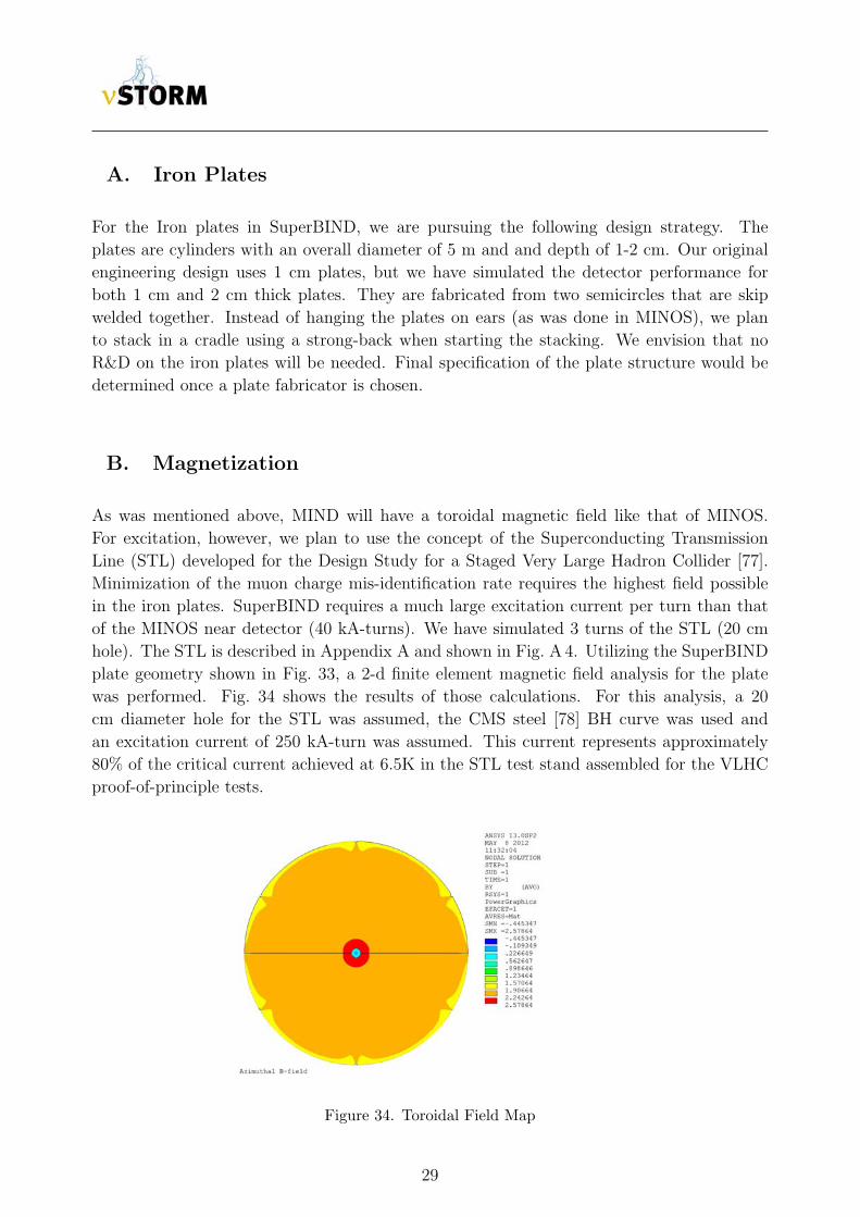
B. Magnetization

As was mentioned above, MIND will have a toroidal magnetic field like that of MINOS.

For excitation, however, we plan to use the concept of the Superconducting Transmission

Line (STL) developed for the Design Study for a Staged Very Large Hadron Collider [77].

Minimization of the muon charge mis-identification rate requires the highest field possible

in the iron plates. SuperBIND requires a much large excitation current per turn than that

of the MINOS near detector (40 kA-turns). We have simulated 3 turns of the STL (20 cm

hole). The STL is described in Appendix A and shown in Fig. A 4. Utilizing the SuperBIND

plate geometry shown in Fig. 33, a 2-d finite element magnetic field analysis for the plate

was performed. Fig. 34 shows the results of those calculations. For this analysis, a 20

cm diameter hole for the STL was assumed, the CMS steel [78] BH curve was used and

an excitation current of 250 kA-turn was assumed. This current represents approximately

80% of the critical current achieved at 6.5K in the STL test stand assembled for the VLHC

proof-of-principle tests.

Figure 34. Toroidal Field Map

29

C. Detector planes

1. Scintillator

Particle detection using extruded scintillator and optical fibers is a mature technology. MI-

NOS has shown that co-extruded solid scintillator with embedded wavelength shifting (WLS)

fibers and PMT readout produces adequate light for MIP tracking and that it can be manu-

factured with excellent quality control and uniformity in an industrial setting. Many exper-

iments use this same technology for the active elements of their detectors, such as the K2K

Scibar [79], the T2K INGRID, P0D, and ECAL [80] and the Double-Chooz cosmic-ray veto

detectors [81].

Our initial concept for the readout planes for SuperBIND is to have both an x and a y

view between each plate. The simulations done to date have assumed a scintillator extrusion

profile that is 1.0 × 1.0 cm2. This gives both the required point resolution and light yield.

2. Scintillator extrusions

The existing SuperBIND simulations have assumed that the readout planes will use an

extrusion that is 1.0 × 1.0 cm2. A 1 mm hole down the centre of the extrusion is provided

for insertion of the wavelength shifting fiber. This is a relatively simple part to manufacture

and has already been fabricated in a similar form for a number of small-scale applications.

The scintillator strips will consist of an extruded polystyrene core doped with blue-emitting

fluorescent compounds, a co-extruded TiO2 outer layer for reflectivity, and a hole in the

middle for a WLS fiber. Dow Styron 665 W polystyrene pellets are doped with PPO (1%

by weight) and POPOP (0.03% by weight). The strips have a white, co-extruded, 0.25

mm thick TiO2 reflective coating. This layer is introduced in a single step as part of a co-

extrusion process. The composition of this coating is 15% TiO2 in polystyrene. In addition

to its reflectivity properties, the layer facilitates the assembly of the scintillator strips into

modules. The ruggedness of this coating enables the direct gluing of the strips to each other

and to the module skins which results in labour and time savings. This process has now

been used in a number of experiments.

D. Photo-detector

Given the rapid development in recent years of solid-state photodetectors based on Geiger

mode operation of silicon avalanche photodiodes, we have chosen this technology for Su-

perBIND. Although various names are used for this technology, we will use silicon photo-

multiplier or SiPM.

30

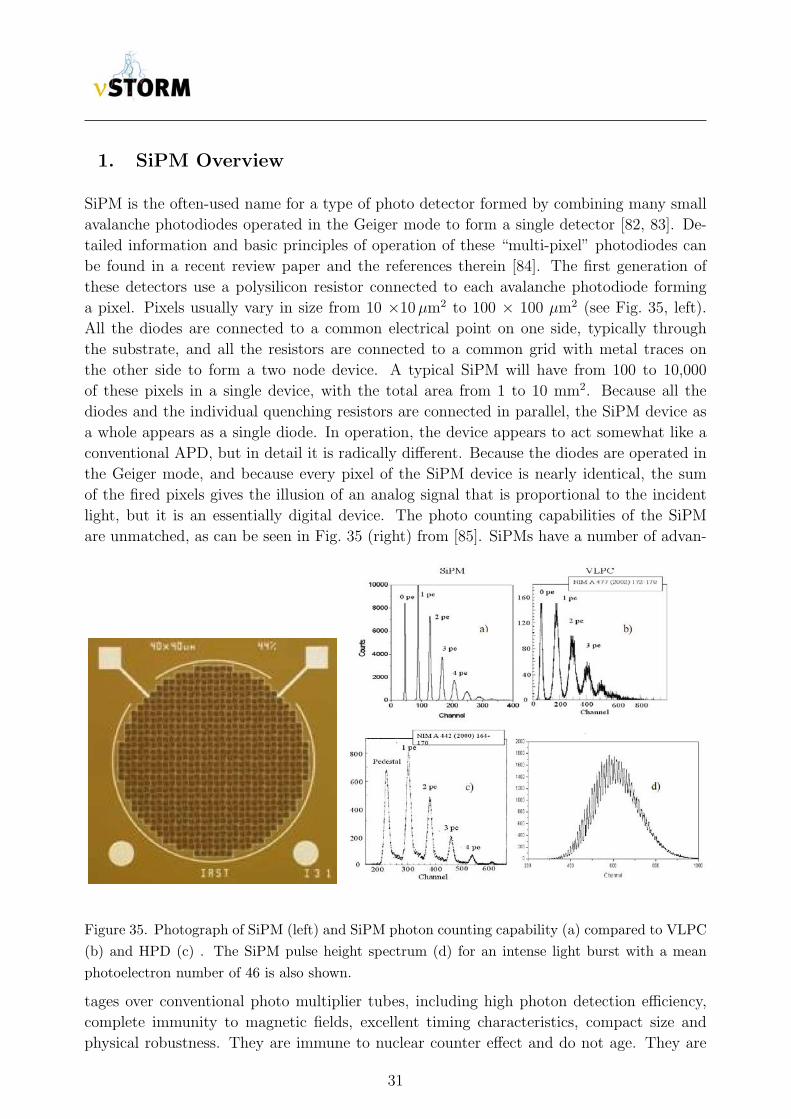
1. SiPM Overview

SiPM is the often-used name for a type of photo detector formed by combining many small

avalanche photodiodes operated in the Geiger mode to form a single detector [82, 83]. De-

tailed information and basic principles of operation of these “multi-pixel” photodiodes can

be found in a recent review paper and the references therein [84]. The first generation of

these detectors use a polysilicon resistor connected to each avalanche photodiode forming

a pixel. Pixels usually vary in size from 10 ×10µm2 to 100 × 100 µm2 (see Fig. 35, left).

All the diodes are connected to a common electrical point on one side, typically through

the substrate, and all the resistors are connected to a common grid with metal traces on

the other side to form a two node device. A typical SiPM will have from 100 to 10,000

of these pixels in a single device, with the total area from 1 to 10 mm2. Because all the

diodes and the individual quenching resistors are connected in parallel, the SiPM device as

a whole appears as a single diode. In operation, the device appears to act somewhat like a

conventional APD, but in detail it is radically different. Because the diodes are operated in

the Geiger mode, and because every pixel of the SiPM device is nearly identical, the sum

of the fired pixels gives the illusion of an analog signal that is proportional to the incident

light, but it is an essentially digital device. The photo counting capabilities of the SiPM

are unmatched, as can be seen in Fig. 35 (right) from [85]. SiPMs have a number of advan-

Figure 35. Photograph of SiPM (left) and SiPM photon counting capability (a) compared to VLPC

(b) and HPD (c) . The SiPM pulse height spectrum (d) for an intense light burst with a mean

photoelectron number of 46 is also shown.

tages over conventional photo multiplier tubes, including high photon detection efficiency,

complete immunity to magnetic fields, excellent timing characteristics, compact size and

physical robustness. They are immune to nuclear counter effect and do not age. They are

31

particularly well suited to applications where optical fibers are used, as the natural size of

the SiPM is comparable to that of fibers. But the most important single feature of the SiPM

is that it can be manufactured in standard microelectronics facilities using well established

processing. This means that huge numbers of devices can be produced without any manual

labor, making the SiPMs very economical as the number of devices grows. Furthermore, it

is possible to integrate the electronics into the SiPM itself, which reduces cost and improves

performance. Initial steps have been taken in this direction, though most current SiPMs do

not have integrated electronics. But it is widely recognized that this is the approach that

makes sense in the long run for many applications. It improves performance and reduces

cost, and can be tailored to a specific application. As the use of SiPMs spreads, so will the

use of custom SiPM with integrated electronics, just as ASICs have superseded standard

logic in micro electronics.

The photon detection efficiency (PDE) of a SiPM is the product of 3 factors:

PDE = QE · εGeiger · εpixel, (1)

where QE is the wavelength-dependent quantum efficiency, εGeiger is the probability to initi-

ate the Geiger discharge by a photoelectron, and εpixel is the fraction of the total photodiode

area occupied by sensitive pixels. The bias voltage affects one parameter in the expres-

sion (1), εGeiger. The geometrical factor εpixel is completely determined by the photodiode

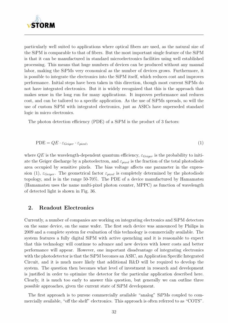
topology, and is in the range 50-70%. The PDE of a device manufactured by Hamamatsu

(Hamamatsu uses the name multi-pixel photon counter, MPPC) as function of wavelength

of detected light is shown in Fig. 36.

2. Readout Electronics

Currently, a number of companies are working on integrating electronics and SiPM detectors

on the same device, on the same wafer. The first such device was announced by Philips in

2009 and a complete system for evaluation of this technology is commercially available. The

system features a fully digital SiPM with active quenching and it is reasonable to expect

that this technology will continue to advance and new devices with lower costs and better

performance will appear. However, one important disadvantage of integrating electronics

with the photodetector is that the SiPM becomes an ASIC, an Application Specific Integrated

Circuit, and it is much more likely that additional R&D will be required to develop the

system. The question then becomes what level of investment in research and development

is justified in order to optimize the detector for the particular application described here.

Clearly, it is much too early to answer this question, but generally we can outline three

possible approaches, given the current state of SiPM development.

The first approach is to pursue commercially available “analog” SiPMs coupled to com-

mercially available, “off the shelf” electronics. This approach is often referred to as “COTS”.

32

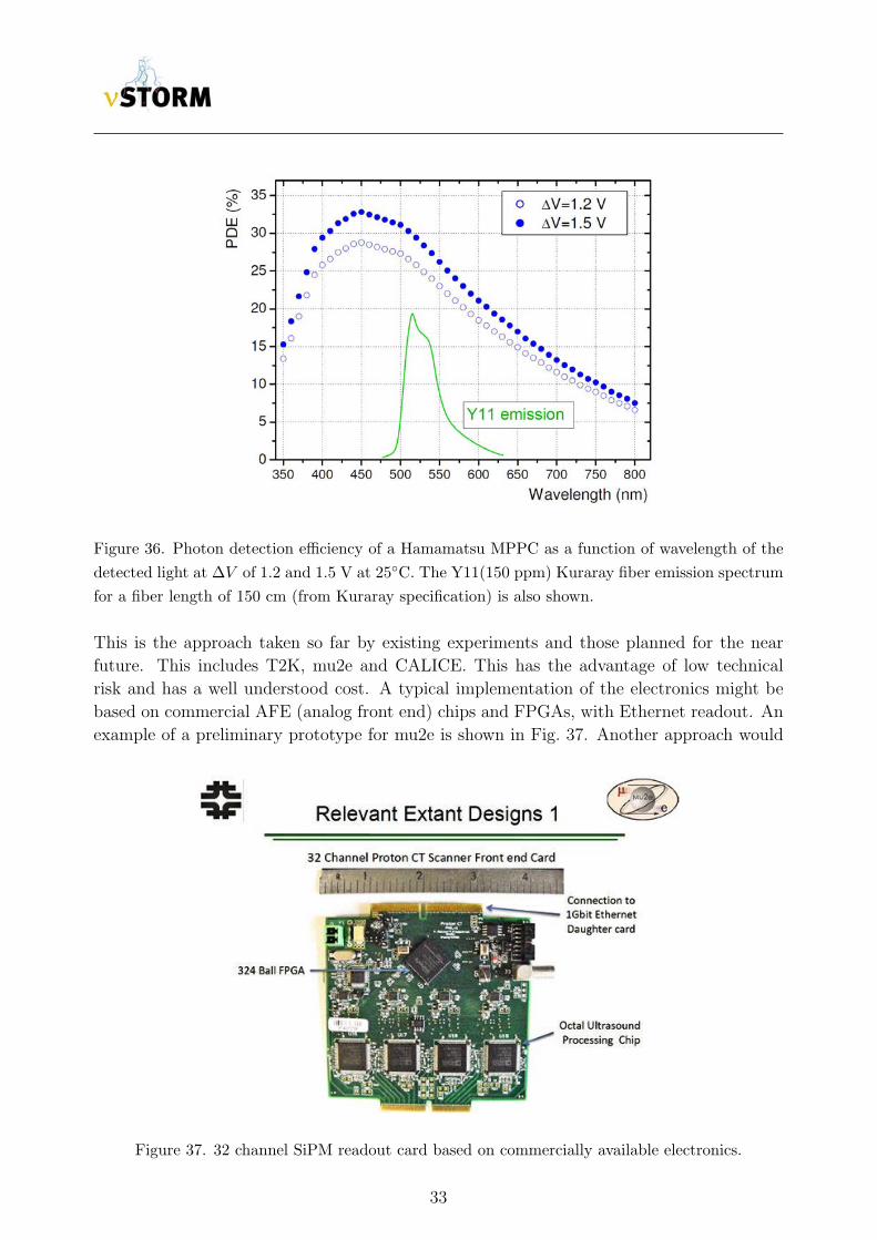
Figure 36. Photon detection efficiency of a Hamamatsu MPPC as a function of wavelength of the

detected light at ∆V of 1.2 and 1.5 V at 25C. The Y11(150 ppm) Kuraray fiber emission spectrum

for a fiber length of 150 cm (from Kuraray specification) is also shown.

This is the approach taken so far by existing experiments and those planned for the near

future. This includes T2K, mu2e and CALICE. This has the advantage of low technical

risk and has a well understood cost. A typical implementation of the electronics might be

based on commercial AFE (analog front end) chips and FPGAs, with Ethernet readout. An

example of a preliminary prototype for mu2e is shown in Fig. 37. Another approach would

Figure 37. 32 channel SiPM readout card based on commercially available electronics.

33

be to adopt existing SiPMs to an existing ASIC designed specifically for SiPMs. This is not

the same as developing a custom ASIC, as these devices already exist for some other experi-

ments. There are many similarities between different experiments in high energy physics and

the popularity and interest in SiPMs is driving development for various applications. Some

examples of ASICs that have been used (or are being developed for use) with SiPMs are the

TriP-t (developed at Fermilab for Dzero, now used by T2K for SiPM readout), TARGET

(developed for Cherenkov Telescope Array) [86] as well as the EASIROC, the SPIROC and

their derivative chips that were developed by the Omega group at IN2P3 in Orsay. The

third approach is to develop a custom solution, using either analog or digital SiPMs. This

approach could potentially significantly reduce the per channel cost of both the photodetec-

tor and electronics, but involves higher technical risk and requires larger initial investment.

This is clearly the best approach for a sufficiently large detector system, but more resources

would need to be devoted to make a specific proposal for a custom SiPM development. One

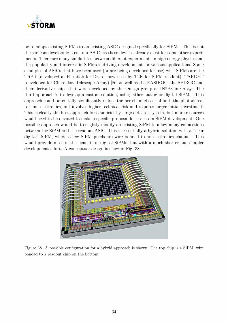
possible approach would be to slightly modify an existing SiPM to allow many connections

between the SiPM and the readout ASIC. This is essentially a hybrid solution with a “near

digital” SiPM, where a few SiPM pixels are wire bonded to an electronics channel. This

would provide most of the benefits of digital SiPMs, but with a much shorter and simpler

development effort. A conceptual design is show in Fig. 38

Figure 38. A possible configuration for a hybrid approach is shown. The top chip is a SiPM, wire

bonded to a readout chip on the bottom.

34

V. NEAR DETECTORS

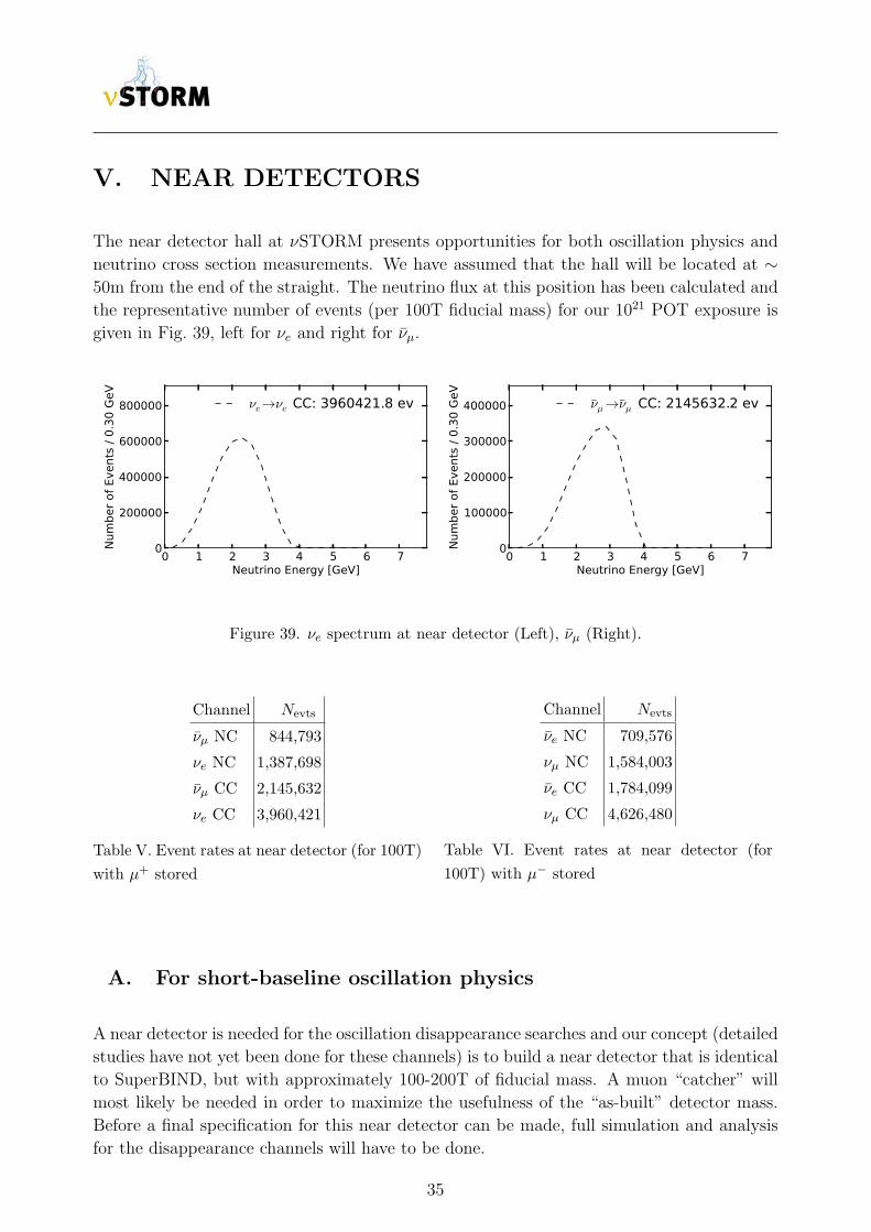
The near detector hall at νSTORM presents opportunities for both oscillation physics and

neutrino cross section measurements. We have assumed that the hall will be located at ∼50m from the end of the straight. The neutrino flux at this position has been calculated and

the representative number of events (per 100T fiducial mass) for our 1021 POT exposure is

given in Fig. 39, left for νe and right for νµ.

Figure 39. νe spectrum at near detector (Left), νµ (Right).

Channel Nevts

νµ NC 844,793

νe NC 1,387,698

νµ CC 2,145,632

νe CC 3,960,421

Table V. Event rates at near detector (for 100T)

with µ+ stored

Channel Nevts

νe NC 709,576

νµ NC 1,584,003

νe CC 1,784,099

νµ CC 4,626,480

Table VI. Event rates at near detector (for

100T) with µ− stored

A. For short-baseline oscillation physics

A near detector is needed for the oscillation disappearance searches and our concept (detailed

studies have not yet been done for these channels) is to build a near detector that is identical

to SuperBIND, but with approximately 100-200T of fiducial mass. A muon “catcher” will

most likely be needed in order to maximize the usefulness of the “as-built” detector mass.

Before a final specification for this near detector can be made, full simulation and analysis

for the disappearance channels will have to be done.

35

B. HIRESMNU: A High-Resolution Detector for ν interaction

studies

Precision measurements of neutrino-interactions at the near-detector (ND) are necessary to

ensure the highest possible sensitivity for neutrino oscillation studies (both for νSTORM

and for any future long-baseline neutrino oscillation experiment). Regardless of the process

under study — νµ → νe appearance or νµ → νe disappearance — the systematic error should

be less than the corresponding statistical error. A near detector concept which will well suit

this purpose is the high resolution detector, HIRESMNU, proposed for the LBNE project

[87]. It can fulfill four principal goals:

1. Measurement of the absolute and the relative abundance of the four species of neu-

trinos, νµ, νµ, νe, νe as a function of energy (Eν). Accurate determination of the angle

and the momentum of the electron in neutrino-electron neutral current interaction will

provide the absolute flux.

2. Determination of the absolute Eν-scale, a factor which determines value of the

oscillation-parameter ∆m2.

3. Determination of π’s and π+/π−’s produced in the NC and CC interactions. The

pions are the predominant source of background for any oscillation study.

4. Measurement of ν-Nucleus cross-section where the nuclear target will be that of the

far-detector. The cross-section measurements of exclusive and inclusive CC and NC

processes will furnish a rich panoply of physics relevant for most neutrino research.

Knowing the cross sections at the Eν typical of the νSTORM beam is essential for

predicting both the signal and the background.

Figure 40 shows a schematic of this the HIRESMNU design. The architecture [87] derives

from the experience of NOMAD [88]. It embeds a 4× 4× 7 m3 STT and a surrounding 4π

electromagnetic calorimeter (ECAL) in a dipole magnet with B ≃ 0.4 T. Downstream of the

magnet and additionally within the magnet yoke are detectors for muon identification. The

STT will have a low average density similar to liquid hydrogen, about 0.1 gm/cm3, which

is essential for the momentum determination and ID of electrons, protons, and pions. The

foil layers interleaved with the straw tubes contribute most of the 7 ton fiducial mass. The

foil layers serve both as the mass on which the neutrinos will interact and as generators of

transition radiation (TR), which aids in electron identification. Its depth in radiation lengths

is sufficient for 50% of the photons from π decay to be observed as e+e− pairs, which delivers

superior resolution compared with conversions in the ECAL. Layers of nuclear-targets will

be deployed at the upstream end of the STT for the determination of cross sections on these

materials. The HIRESMNU delivers the most sensitive systematic constraints as studied

within the context of future long-baseline ν experiments. The systematic studies include

ν-electron scattering, quasi-elastic interactions, νe/νe-CC, neutral-current identification, π

detection, etc. The quoted dimensions, mass, and segmentation of HIRESMNU will be

further optimized for νSTORM as the proposal evolves.

36

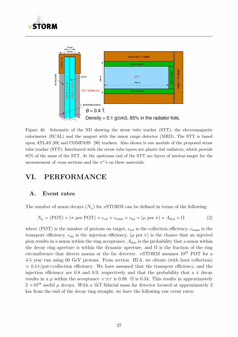
Figure 40. Schematic of the ND showing the straw tube tracker (STT), the electromagnetic

calorimeter (ECAL) and the magnet with the muon range detector (MRD). The STT is based

upon ATLAS [89] and COMPASS [90] trackers. Also shown is one module of the proposed straw

tube tracker (STT). Interleaved with the straw tube layers are plastic foil radiators, which provide

85% of the mass of the STT. At the upstream end of the STT are layers of nuclear-target for the

measurement of cross sections and the π’s on these materials.

VI. PERFORMANCE

A. Event rates

The number of muon decays (Nµ) for νSTORM can be defined in terms of the following:

Nµ = (POT)× (π per POT)× ϵcol × ϵtrans × ϵinj × (µ per π)× Adyn × Ω (2)

where (POT) is the number of protons on target, ϵcol is the collection efficiency, ϵtrans is the

transport efficiency, ϵinj is the injection efficiency, (µ per π) is the chance that an injected

pion results in a muon within the ring acceptance, Adyn is the probability that a muon within

the decay ring aperture is within the dynamic aperture, and Ω is the fraction of the ring

circumference that directs muons at the far detector. νSTORM assumes 1021 POT for a

4-5 year run using 60 GeV protons. From section IIIA, we obtain (with horn collection)

≃ 0.1π/pot×collection efficiency. We have assumed that the transport efficiency, and the

injection efficiency are 0.8 and 0.9, respectively and that the probability that a π decay

results in a µ within the acceptance ×γcτ is 0.08. Ω is 0.34. This results in approximately

2 ×1018 useful µ decays. With a 1kT fiducial mass far detector located at approximately 2

km from the end of the decay ring straight, we have the following raw event rates:

37

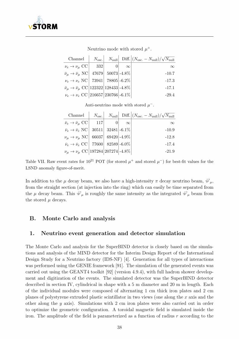
Neutrino mode with stored µ+.

Channel Nosc. Nnull Diff. (Nosc. −Nnull)/√Nnull

νe → νµ CC 332 0 ∞ ∞νµ → νµ NC 47679 50073 -4.8% -10.7

νe → νe NC 73941 78805 -6.2% -17.3

νµ → νµ CC 122322 128433 -4.8% -17.1

νe → νe CC 216657 230766 -6.1% -29.4

Anti-neutrino mode with stored µ−.

Channel Nosc. Nnull Diff. (Nosc. −Nnull)/√Nnull

νe → νµ CC 117 0 ∞ ∞νe → νe NC 30511 32481 -6.1% -10.9

νµ → νµ NC 66037 69420 -4.9% -12.8

νe → νe CC 77600 82589 -6.0% -17.4

νµ → νµ CC 197284 207274 -4.8% -21.9

Table VII. Raw event rates for 1021 POT (for stored µ+ and stored µ−) for best-fit values for the

LSND anomaly figure-of-merit.

In addition to the µ decay beam, we also have a high-intensity π decay neutrino beam, ν µ,

from the straight section (at injection into the ring) which can easily be time separated from

the µ decay beam. This ν µ is roughly the same intensity as the integrated ν µ beam from

the stored µ decays.

B. Monte Carlo and analysis

1. Neutrino event generation and detector simulation

The Monte Carlo and analysis for the SuperBIND detector is closely based on the simula-

tions and analysis of the MIND detector for the Interim Design Report of the International

Design Study for a Neutrino factory (IDS-NF) [4]. Generation for all types of interactions

was performed using the GENIE framework [91]. The simulation of the generated events was

carried out using the GEANT4 toolkit [92] (version 4.9.4), with full hadron shower develop-

ment and digitization of the events. The simulated detector was the SuperBIND detector

described in section IV, cylindrical in shape with a 5 m diameter and 20 m in length. Each

of the individual modules were composed of alternating 1 cm thick iron plates and 2 cm

planes of polystyrene extruded plastic scintillator in two views (one along the x axis and the

other along the y axis). Simulations with 2 cm iron plates were also carried out in order

to optimize the geometric configuration. A toroidal magnetic field is simulated inside the

iron. The amplitude of the field is parameterized as a function of radius r according to the

38

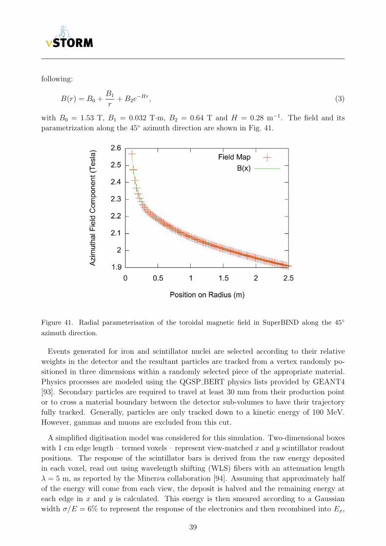
following:

B(r) = B0 +B1

r+ B2e

−Hr, (3)

with B0 = 1.53 T, B1 = 0.032 T·m, B2 = 0.64 T and H = 0.28 m−1. The field and its

parametrization along the 45 azimuth direction are shown in Fig. 41.

Figure 41. Radial parameterisation of the toroidal magnetic field in SuperBIND along the 45

azimuth direction.

Events generated for iron and scintillator nuclei are selected according to their relative

weights in the detector and the resultant particles are tracked from a vertex randomly po-

sitioned in three dimensions within a randomly selected piece of the appropriate material.

Physics processes are modeled using the QGSP BERT physics lists provided by GEANT4

[93]. Secondary particles are required to travel at least 30 mm from their production point

or to cross a material boundary between the detector sub-volumes to have their trajectory

fully tracked. Generally, particles are only tracked down to a kinetic energy of 100 MeV.

However, gammas and muons are excluded from this cut.

A simplified digitisation model was considered for this simulation. Two-dimensional boxes

with 1 cm edge length – termed voxels – represent view-matched x and y scintillator readout

positions. The response of the scintillator bars is derived from the raw energy deposited

in each voxel, read out using wavelength shifting (WLS) fibers with an attenuation length

λ = 5 m, as reported by the Minerνa collaboration [94]. Assuming that approximately half

of the energy will come from each view, the deposit is halved and the remaining energy at

each edge in x and y is calculated. This energy is then smeared according to a Gaussian

width σ/E = 6% to represent the response of the electronics and then recombined into Ex,

39

Ey and total energy = Ex+Ey energy deposited per voxel. An output wavelength of 525 nm,

a photo-detector quantum efficiency of ∼30% and a threshold of 4.7 photo electrons (pe) per

view (as in MINOS [76]) were assumed. Any voxel view that is not above the threshold is

cut.

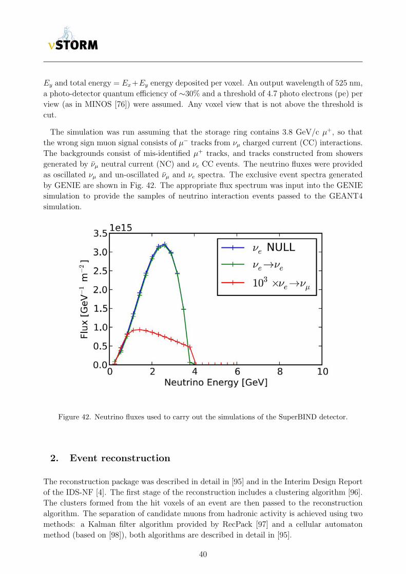
The simulation was run assuming that the storage ring contains 3.8 GeV/c µ+, so that

the wrong sign muon signal consists of µ− tracks from νµ charged current (CC) interactions.

The backgrounds consist of mis-identified µ+ tracks, and tracks constructed from showers

generated by νµ neutral current (NC) and νe CC events. The neutrino fluxes were provided

as oscillated νµ and un-oscillated νµ and νe spectra. The exclusive event spectra generated

by GENIE are shown in Fig. 42. The appropriate flux spectrum was input into the GENIE

simulation to provide the samples of neutrino interaction events passed to the GEANT4

simulation.

Figure 42. Neutrino fluxes used to carry out the simulations of the SuperBIND detector.

2. Event reconstruction

The reconstruction package was described in detail in [95] and in the Interim Design Report

of the IDS-NF [4]. The first stage of the reconstruction includes a clustering algorithm [96].

The clusters formed from the hit voxels of an event are then passed to the reconstruction

algorithm. The separation of candidate muons from hadronic activity is achieved using two

methods: a Kalman filter algorithm provided by RecPack [97] and a cellular automaton

method (based on [98]), both algorithms are described in detail in [95].

40

Fitting of the muon candidates proceeds using a Kalman filter to fit a helix to the can-

didate, using an initial seed estimated from the path length of the muon track, using the

Continuous Slowing Down Approximation (CSDA [99]), and then refitting any successes.

Neutrino energy is generally reconstructed as the sum of the muon and hadronic energies,

with hadronic reconstruction currently performed using a smear on the true quantities as

described in reference [95]. The reconstruction of the hadronic energy Ehad (in GeV) assumes

a resolution δEhad from the MINOS CalDet testbeam [76, 100] (although we believe that

SuperBIND will do better):

δEhad

Ehad

=0.55√Ehad

⊕ 0.03. (4)

The hadronic shower direction vector is also smeared according to the angular resolution

found by the Monolith test-beam [101]:

δθhad =10.4√Ehad

⊕ 10.1

Ehad

. (5)

In the case of QE interactions, where there is no hadronic jet, the neutrino energy recon-

struction was carried out using the formula:

Eν =mNEµ +

12

(m2

N ′ −m2µ −m2

N

)mN − Eµ + |pµ| cosϑ

; (6)

where ϑ is the angle between the muon momentum vector and the beam direction, mN is

the mass of the initial state nucleon, and mN ′ is the mass of the outgoing nucleon for the

interactions νµ + n → µ− + p and νµ + p → µ+ + n (see for example [102]).

The iron plate thickness of the detector was studied from the point of view of muon charge

identification efficiency. The charge selection efficiency was studied using 1 cm iron plates

and 2 cm iron plates. By doubling the thickness of the iron plate, we effectively increase the

effective magnetic field between measurements by 50% so the net charge selection efficiency

increases, at the expense of a small increase in the threshold. Both of these effects were

studied in detail in the following data analysis section.

C. Data Analysis

The basis for the νe → νµ analysis closely follows the one for the MIND detector at a

Neutrino Factory [4], but was adapted for the lower muon energy of 3.8 GeV. The cuts to

reject charged current (CC) and neutral current (NC) backgrounds are organized as follows:

• Successful reconstruction.

• Fiducial volume cut.

• Maximum momentum cut.

• Fitted proportion of hits allocated to the muon track.

41

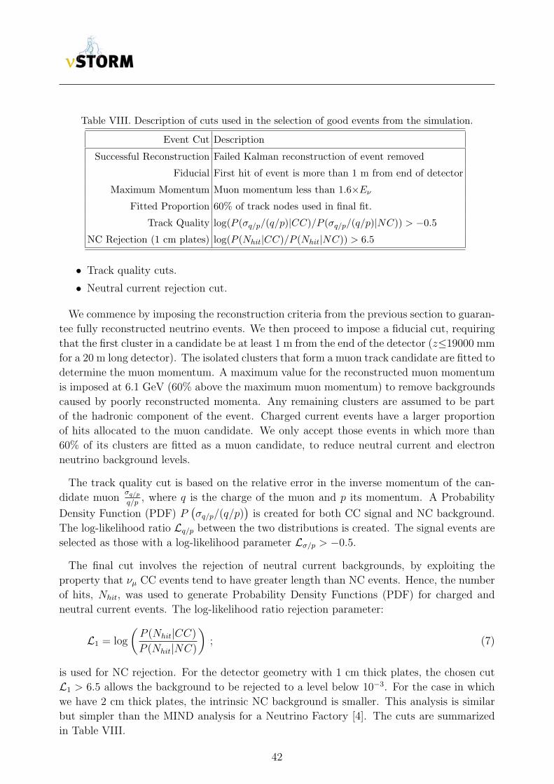
Table VIII. Description of cuts used in the selection of good events from the simulation.

Event Cut Description

Successful Reconstruction Failed Kalman reconstruction of event removed

Fiducial First hit of event is more than 1 m from end of detector

Maximum Momentum Muon momentum less than 1.6×Eν

Fitted Proportion 60% of track nodes used in final fit.

Track Quality log(P (σq/p/(q/p)|CC)/P (σq/p/(q/p)|NC)) > −0.5

NC Rejection (1 cm plates) log(P (Nhit|CC)/P (Nhit|NC)) > 6.5

• Track quality cuts.

• Neutral current rejection cut.

We commence by imposing the reconstruction criteria from the previous section to guaran-

tee fully reconstructed neutrino events. We then proceed to impose a fiducial cut, requiring

that the first cluster in a candidate be at least 1 m from the end of the detector (z≤19000 mm

for a 20 m long detector). The isolated clusters that form a muon track candidate are fitted to

determine the muon momentum. A maximum value for the reconstructed muon momentum

is imposed at 6.1 GeV (60% above the maximum muon momentum) to remove backgrounds

caused by poorly reconstructed momenta. Any remaining clusters are assumed to be part

of the hadronic component of the event. Charged current events have a larger proportion

of hits allocated to the muon candidate. We only accept those events in which more than

60% of its clusters are fitted as a muon candidate, to reduce neutral current and electron

neutrino background levels.

The track quality cut is based on the relative error in the inverse momentum of the can-

didate muonσq/p

q/p, where q is the charge of the muon and p its momentum. A Probability

Density Function (PDF) P(σq/p/(q/p)

)is created for both CC signal and NC background.

The log-likelihood ratio Lq/p between the two distributions is created. The signal events are

selected as those with a log-likelihood parameter Lσ/p > −0.5.

The final cut involves the rejection of neutral current backgrounds, by exploiting the

property that νµ CC events tend to have greater length than NC events. Hence, the number

of hits, Nhit, was used to generate Probability Density Functions (PDF) for charged and

neutral current events. The log-likelihood ratio rejection parameter:

L1 = log

(P (Nhit|CC)

P (Nhit|NC)

); (7)

is used for NC rejection. For the detector geometry with 1 cm thick plates, the chosen cut

L1 > 6.5 allows the background to be rejected to a level below 10−3. For the case in which

we have 2 cm thick plates, the intrinsic NC background is smaller. This analysis is similar

but simpler than the MIND analysis for a Neutrino Factory [4]. The cuts are summarized

in Table VIII.

42

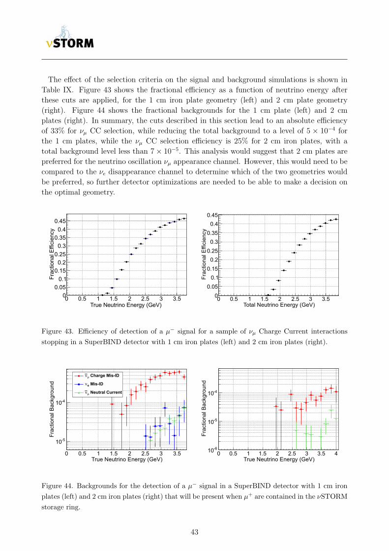
The effect of the selection criteria on the signal and background simulations is shown in

Table IX. Figure 43 shows the fractional efficiency as a function of neutrino energy after

these cuts are applied, for the 1 cm iron plate geometry (left) and 2 cm plate geometry

(right). Figure 44 shows the fractional backgrounds for the 1 cm plate (left) and 2 cm

plates (right). In summary, the cuts described in this section lead to an absolute efficiency

of 33% for νµ CC selection, while reducing the total background to a level of 5 × 10−4 for

the 1 cm plates, while the νµ CC selection efficiency is 25% for 2 cm iron plates, with a

total background level less than 7× 10−5. This analysis would suggest that 2 cm plates are

preferred for the neutrino oscillation νµ appearance channel. However, this would need to be

compared to the νe disappearance channel to determine which of the two geometries would

be preferred, so further detector optimizations are needed to be able to make a decision on

the optimal geometry.

True Neutrino Energy (GeV)0 0.5 1 1.5 2 2.5 3 3.5

Fra

ctio

nal E

ffici

ency

00.05

0.10.15

0.20.25

0.30.35

0.40.45

Total Neutrino Energy (GeV)0 0.5 1 1.5 2 2.5 3 3.5

Frac

tiona

l Effi

cien

cy

00.05

0.10.15

0.20.25

0.30.35

0.40.45

Figure 43. Efficiency of detection of a µ− signal for a sample of νµ Charge Current interactions

stopping in a SuperBIND detector with 1 cm iron plates (left) and 2 cm iron plates (right).

True Neutrino Energy (GeV)0 0.5 1 1.5 2 2.5 3 3.5

Frac

tiona

l Bac

kgro

und

-510

-410

Charge Mis-IDµν

Mis-IDeν

Neutral Currentµν

True Neutrino Energy (GeV)0 0.5 1 1.5 2 2.5 3 3.5 4

Fra

ctio

nal B

ackg

roun

d

-610

-510

-410

Figure 44. Backgrounds for the detection of a µ− signal in a SuperBIND detector with 1 cm iron

plates (left) and 2 cm iron plates (right) that will be present when µ+ are contained in the νSTORM

storage ring.

43

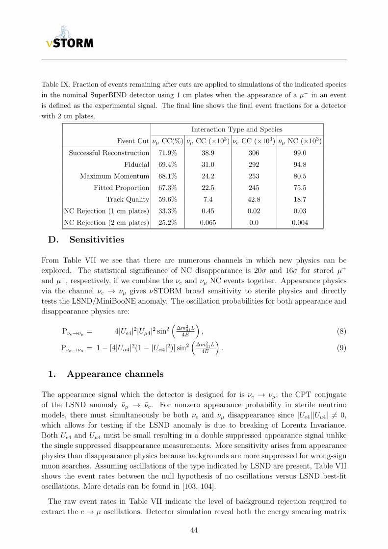
Table IX. Fraction of events remaining after cuts are applied to simulations of the indicated species

in the nominal SuperBIND detector using 1 cm plates when the appearance of a µ− in an event

is defined as the experimental signal. The final line shows the final event fractions for a detector

with 2 cm plates.

Interaction Type and Species

Event Cut νµ CC(%) νµ CC (×103) νe CC (×103) νµ NC (×103)

Successful Reconstruction 71.9% 38.9 306 99.0

Fiducial 69.4% 31.0 292 94.8

Maximum Momentum 68.1% 24.2 253 80.5

Fitted Proportion 67.3% 22.5 245 75.5

Track Quality 59.6% 7.4 42.8 18.7

NC Rejection (1 cm plates) 33.3% 0.45 0.02 0.03

NC Rejection (2 cm plates) 25.2% 0.065 0.0 0.004

D. Sensitivities

From Table VII we see that there are numerous channels in which new physics can be

explored. The statistical significance of NC disappearance is 20σ and 16σ for stored µ+

and µ−, respectively, if we combine the νe and νµ NC events together. Appearance physics

via the channel νe → νµ gives νSTORM broad sensitivity to sterile physics and directly

tests the LSND/MiniBooNE anomaly. The oscillation probabilities for both appearance and

disappearance physics are:

Pνe→νµ = 4|Ue4|2|Uµ4|2 sin2(

∆m241L

4E

), (8)

Pνα→να = 1− [4|Uα4|2(1− |Uα4|2)] sin2(

∆m241L

4E

). (9)

1. Appearance channels

The appearance signal which the detector is designed for is νe → νµ; the CPT conjugate

of the LSND anomaly νµ → νe. For nonzero appearance probability in sterile neutrino

models, there must simultaneously be both νe and νµ disappearance since |Ue4||Uµ4| = 0,

which allows for testing if the LSND anomaly is due to breaking of Lorentz Invariance.

Both Ue4 and Uµ4 must be small resulting in a double suppressed appearance signal unlike

the single suppressed disappearance measurements. More sensitivity arises from appearance

physics than disappearance physics because backgrounds are more suppressed for wrong-sign

muon searches. Assuming oscillations of the type indicated by LSND are present, Table VII

shows the event rates between the null hypothesis of no oscillations versus LSND best-fit

oscillations. More details can be found in [103, 104].

The raw event rates in Table VII indicate the level of background rejection required to

extract the e → µ oscillations. Detector simulation reveal both the energy smearing matrix

44

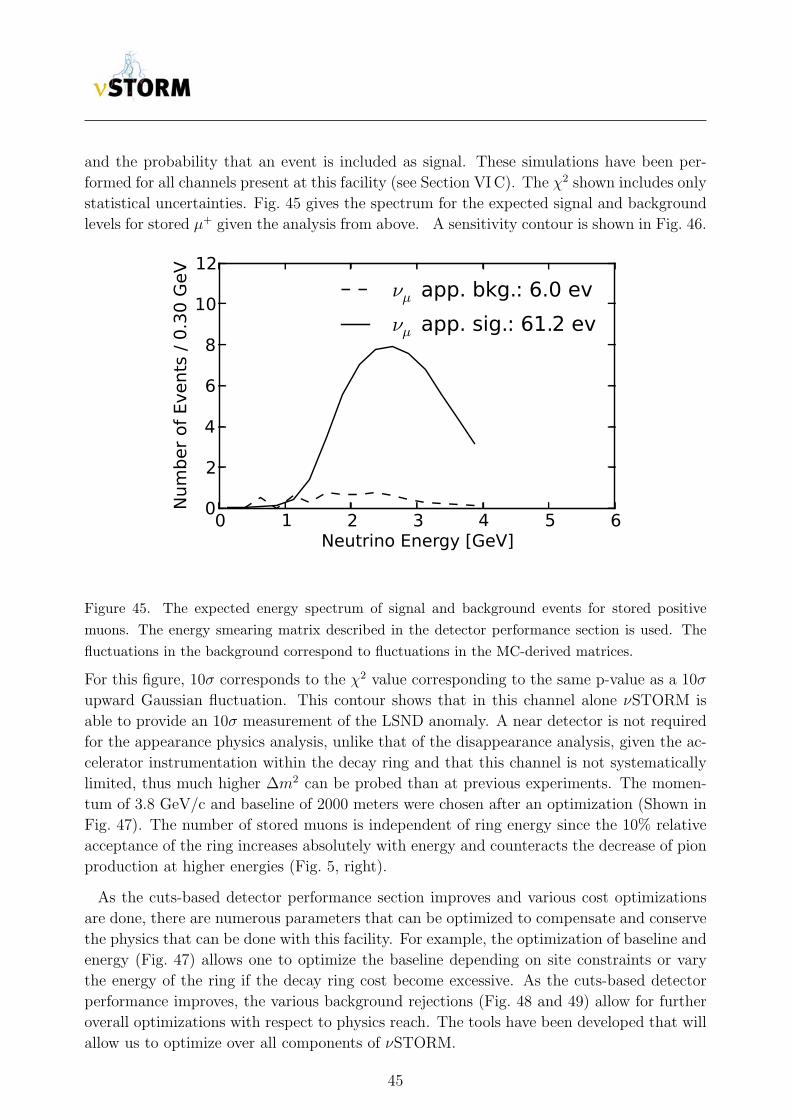
and the probability that an event is included as signal. These simulations have been per-

formed for all channels present at this facility (see Section VIC). The χ2 shown includes only

statistical uncertainties. Fig. 45 gives the spectrum for the expected signal and background

levels for stored µ+ given the analysis from above. A sensitivity contour is shown in Fig. 46.

Figure 45. The expected energy spectrum of signal and background events for stored positive

muons. The energy smearing matrix described in the detector performance section is used. The

fluctuations in the background correspond to fluctuations in the MC-derived matrices.

For this figure, 10σ corresponds to the χ2 value corresponding to the same p-value as a 10σ

upward Gaussian fluctuation. This contour shows that in this channel alone νSTORM is

able to provide an 10σ measurement of the LSND anomaly. A near detector is not required

for the appearance physics analysis, unlike that of the disappearance analysis, given the ac-

celerator instrumentation within the decay ring and that this channel is not systematically

limited, thus much higher ∆m2 can be probed than at previous experiments. The momen-

tum of 3.8 GeV/c and baseline of 2000 meters were chosen after an optimization (Shown in

Fig. 47). The number of stored muons is independent of ring energy since the 10% relative

acceptance of the ring increases absolutely with energy and counteracts the decrease of pion

production at higher energies (Fig. 5, right).

As the cuts-based detector performance section improves and various cost optimizations

are done, there are numerous parameters that can be optimized to compensate and conserve

the physics that can be done with this facility. For example, the optimization of baseline and

energy (Fig. 47) allows one to optimize the baseline depending on site constraints or vary

the energy of the ring if the decay ring cost become excessive. As the cuts-based detector

performance improves, the various background rejections (Fig. 48 and 49) allow for further

overall optimizations with respect to physics reach. The tools have been developed that will

allow us to optimize over all components of νSTORM.

45

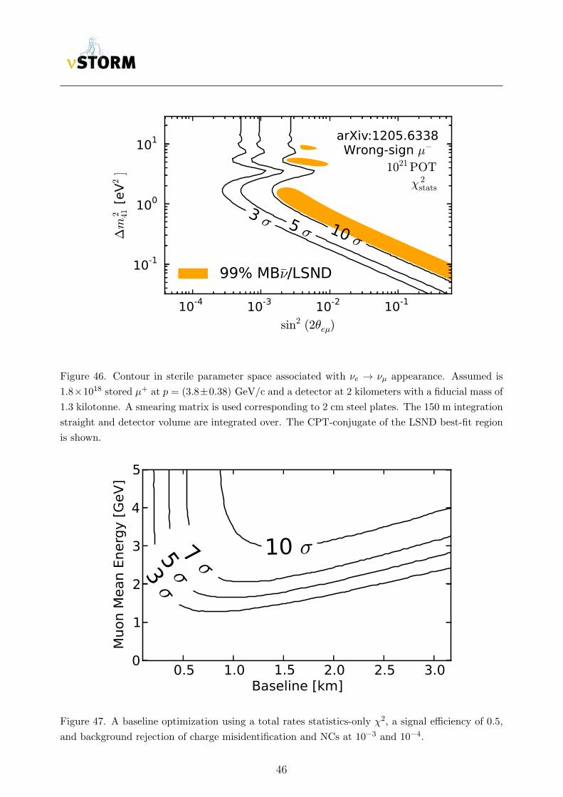
Figure 46. Contour in sterile parameter space associated with νe → νµ appearance. Assumed is

1.8×1018 stored µ+ at p = (3.8±0.38) GeV/c and a detector at 2 kilometers with a fiducial mass of

1.3 kilotonne. A smearing matrix is used corresponding to 2 cm steel plates. The 150 m integration

straight and detector volume are integrated over. The CPT-conjugate of the LSND best-fit region

is shown.

Figure 47. A baseline optimization using a total rates statistics-only χ2, a signal efficiency of 0.5,

and background rejection of charge misidentification and NCs at 10−3 and 10−4.

46

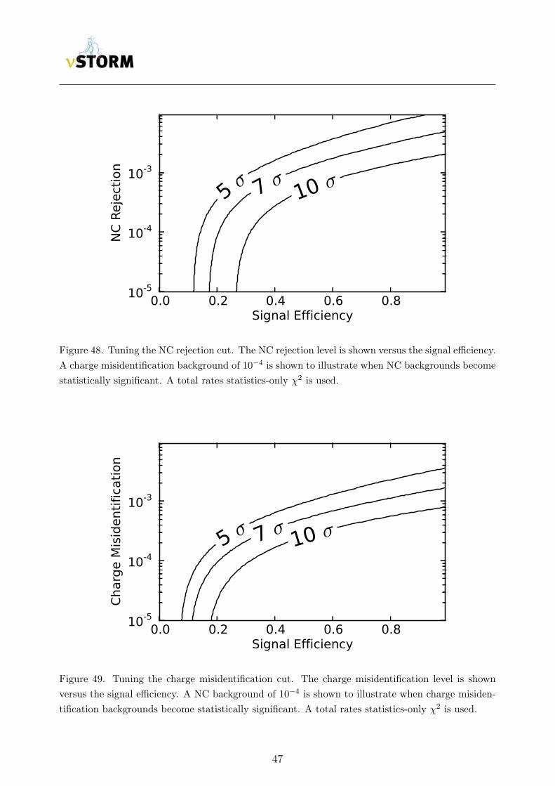
Figure 48. Tuning the NC rejection cut. The NC rejection level is shown versus the signal efficiency.

A charge misidentification background of 10−4 is shown to illustrate when NC backgrounds become

statistically significant. A total rates statistics-only χ2 is used.

Figure 49. Tuning the charge misidentification cut. The charge misidentification level is shown

versus the signal efficiency. A NC background of 10−4 is shown to illustrate when charge misiden-

tification backgrounds become statistically significant. A total rates statistics-only χ2 is used.

47

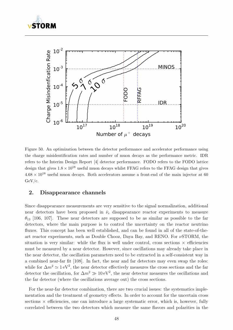
Figure 50. An optimization between the detector performance and accelerator performance using

the charge misidentification rates and number of muon decays as the performance metric. IDR

refers to the Interim Design Report [4] detector performance. FODO refers to the FODO lattice

design that gives 1.8× 1018 useful muon decays whilst FFAG refers to the FFAG design that gives

4.68 × 1018 useful muon decays. Both accelerators assume a front-end of the main injector at 60

GeV/c.

2. Disappearance channels

Since disappearance measurements are very sensitive to the signal normalization, additional

near detectors have been proposed in νe disappearance reactor experiments to measure

θ13 [106, 107]. These near detectors are supposed to be as similar as possible to the far

detectors, where the main purpose is to control the uncertainty on the reactor neutrino

fluxes. This concept has been well established, and can be found in all of the state-of-the-

art reactor experiments, such as Double Chooz, Daya Bay, and RENO. For νSTORM, the

situation is very similar: while the flux is well under control, cross sections × efficiencies

must be measured by a near detector. However, since oscillations may already take place in

the near detector, the oscillation parameters need to be extracted in a self-consistent way in

a combined near-far fit [108]. In fact, the near and far detectors may even swap the roles:

while for ∆m2 1 eV2, the near detector effectively measures the cross sections and the far

detector the oscillation, for ∆m2 10 eV2, the near detector measures the oscillations and

the far detector (where the oscillations average out) the cross sections.

For the near-far detector combination, there are two crucial issues: the systematics imple-

mentation and the treatment of geometry effects. In order to account for the uncertain cross

sections × efficiencies, one can introduce a large systematic error, which is, however, fully

correlated between the two detectors which measure the same flavors and polarities in the

48

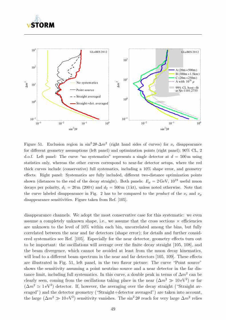
103 102 101 100101

100

101

102

103

sin22Θ

m

2

GLoBES 2012

No systematics

Point source

Straight averaged

Straightdet. averaged

102 101 100101

100

101

102

sin22Θ

m

2

GLoBES 2012

A 20m500m B 300m1.5km C 20m250m Awith 1018 Μ

99 CL bestfitarXiv:1101.2755

Figure 51. Exclusion region in sin2 2θ-∆m2 (right hand sides of curves) for νe disappearance

for different geometry assumptions (left panel) and optimization points (right panel); 90% CL, 2

d.o.f. Left panel: The curve “no systematics” represents a single detector at d = 500m using

statistics only, whereas the other curves correspond to near-far detector setups, where the red

thick curves include (conservative) full systematics, including a 10% shape error, and geometry

effects. Right panel: Systematics are fully included, different two-distance optimization points

shown (distances to the end of the decay straight). Both panels: Eµ = 2GeV, 1019 useful muon

decays per polarity, d1 = 20m (200 t) and d2 = 500m (1 kt), unless noted otherwise. Note that

the curve labeled disappearance in Fig. 2 has to be compared to the product of the νe and νµ

disappearance sensitivities. Figure taken from Ref. [105].

disappearance channels. We adopt the most conservative case for this systematic: we even

assume a completely unknown shape, i.e., we assume that the cross sections × efficiencies

are unknown to the level of 10% within each bin, uncorrelated among the bins, but fully

correlated between the near and far detectors (shape error); for details and further consid-

ered systematics see Ref. [105]. Especially for the near detector, geometry effects turn out

to be important: the oscillations will average over the finite decay straight [105, 108], and

the beam divergence, which cannot be avoided at least from the muon decay kinematics,

will lead to a different beam spectrum in the near and far detectors [105, 109]. These effects

are illustrated in Fig. 51, left panel, in the two flavor picture: The curve “Point source”

shows the sensitivity assuming a point neutrino source and a near detector in the far dis-

tance limit, including full systematics. In this curve, a double peak in terms of ∆m2 can be

clearly seen, coming from the oscillations taking place in the near (∆m2 10 eV2) or far

(∆m2 1 eV2) detector. If, however, the averaging over the decay straight (“Straight av-

eraged”) and the detector geometry (“Straight+detector averaged”) are taken into account,

the large (∆m2 10 eV2) sensitivity vanishes. The sin2 2θ reach for very large ∆m2 relies

49

on the external knowledge of systematics, in this case it is limited by the 10% shape error

As far as the two-baseline optimization is concerned [105], the optimal choice depends

somewhat on the value of ∆m2. This is illustrated in the right panel of Fig. 51, where the

sensitivities for several optimization points are shown. While all of these options perform

equally well for ∆m2 ≃ 1 eV2, larger values of ∆m2 ≃ 1 eV2 prefer shorter distances (from the

end of the decay straight) for the far detector. The optimization point A (20 m+500 m) seems

to be a good compromise between the small and large ∆m2 sensitivities for Eµ = 2GeV.

This is consistent with the optimization for appearance, but somewhat on the lower end of

the optimal baseline range for that. For larger Eµ, slightly longer far detector distances are

preferred, which means that 500m to 800m seems a reasonable distance range. For the near

detector, we find that, in spite of the geometry effects, as short as possible distances are

preferred if the far detector is in that baseline range.

As for the absolute performance, we show in Fig. 51 (right panel) the 99% CL best-fit from

one of the global (anomaly) fits in the literature for comparison. It is clear that νSTORM

can exclude this region for all of the optimization points for ∆m2 . 10 eV2. However, note

that either significantly more than 1018 useful muon decays per polarity (dashed curve) are

needed for that purpose, or muon energies slightly higher than 2 GeV, as it the case in this

document as the central momentum under consideration is 3.8 GeV/c. It can be shown that

the proposed setup then has excellent sensitivity to both νe and νµ disappearance, both for

neutrinos and antineutrinos [105], where the details somewhat depend on the final exposure,

detection efficiency, and systematics treatment.

50

VII. OUTLOOK AND CONCLUSIONS

The physics case for experiments that search for sterile neutrinos is compelling. Beyond

the hints from LSND, MiniBooNE and the reactor νe flux anomaly, sterile neutrinos arise

naturally in many extensions of the Standard Model. They appear in GUT models, in the

seesaw mechanism and may also have an impact in cosmology as they are a possible candidate

for DM or hot DM. Of the 30 or so ideas to search for sterile neutrinos that have recently

been discussed in the literature, νSTORM is the only one that can do all of the following:

• Make a direct test of the LSND and MiniBooNE anomalies.

• Provide stringent constraints for both νe and νµ disappearance to over constrain 3+N

oscillation models and to test the Gallium and reactor anomalies directly.

• Test the CP- and T-conjugated channels as well, in order to obtain the relevant clues

for the underlying physics model, such as CP violation in 3 + 2 models.

We have demonstrated the wide range of science that νSTORM can deliver, ranging from

probing the existence (or non-existence) of sterile neutrinos to neutrino interaction physics in

support of future programs, to the demonstration of and test-bed for novel accelerator tech-

nology. The 10 oscillation channels which νSTORM can probe allows for the study, in depth

and in detail, of the various sterile oscillation scenarios that are theoretically motivated,

while simultaneously being the only proposal that can directly test the LSND anomaly at 10

σ. A source of both electron and muon neutrinos allow for detailed cross section measure-

ments where the electron neutrino cross section will be particularly important for future long

baseline programs. Experimental R&D could also be done using this precisely understood

neutrino source. The program that has been proposed is able to do relevant physics on both

the short term and long term.

A. Proceeding toward a full Proposal

In order to present a full proposal to the laboratory (with a defensible cost estimate), ad-

ditional scientific and engineering effort will be required. We have estimated this effort and

itemize it in Table X.

51

Table X. Estimated effort to produce full proposal

Task ΣFTE

Target Station 0.75

Capture & transport 1.25

Injection 0.25

Decay ring 2

Far Detector (Engineering) 1

Far Detector (Sim & Analysis) 2

Near Detector (Engineering) 1

Near Detector (Sim & Analysis)a 3.5

Costing 1

Total 12.75

aNote: Much of this effort is in complete synergy with the work on-going for the LBNE near detectors. And

what is given here is likely an overestimate for what will be needed for the νSTORM proposal.

52

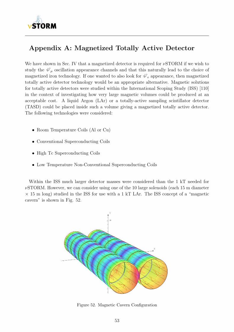
Appendix A: Magnetized Totally Active Detector

We have shown in Sec. IV that a magnetized detector is required for νSTORM if we wish to

study the ν µ oscillation appearance channels and that this naturally lead to the choice of

magnetized iron technology. If one wanted to also look for ν e appearance, then magnetized

totally active detector technology would be an appropriate alternative. Magnetic solutions

for totally active detectors were studied within the International Scoping Study (ISS) [110]

in the context of investigating how very large magnetic volumes could be produced at an

acceptable cost. A liquid Argon (LAr) or a totally-active sampling scintillator detector

(TASD) could be placed inside such a volume giving a magnetized totally active detector.

The following technologies were considered:

• Room Temperature Coils (Al or Cu)

• Conventional Superconducting Coils

• High Tc Superconducting Coils

• Low Temperature Non-Conventional Superconducting Coils

Within the ISS much larger detector masses were considered than the 1 kT needed for

νSTORM. However, we can consider using one of the 10 large solenoids (each 15 m diameter

× 15 m long) studied in the ISS for use with a 1 kT LAr. The ISS concept of a “magnetic

cavern” is shown in Fig. 52.

Figure 52. Magnetic Cavern Configuration

53

1. Conventional Room Temperature Magnets

In order to get adequate field strength with tolerable power dissipation, conventional room-

temperature coils would have to be relatively thick. We first considered Al conductor operat-

ing at 150K. We then determined the amount of conductor necessary to produce a reference

field of only 0.1T. In order to keep the current density at approximately 100A/cm2, 10 lay-

ers of 1 cm2 Al conductor would be required for our 15 m diameter × 15 m long reference

solenoid. Using a $20/kg cost for convention magnets [111], the estimated cost for 1 solenoid

is $5M. The power dissipation (assuming R=1 × 10−8 Ohm-m) is approximately 1 MW.

The operating costs for 1 MW of power would be $1.5M/year (based on typical US power

costs). The cost of the magnet system including 10 years of operation is then $20M. If one

includes the cost of cooling the coils to 150K, the costs increase substantially. Studies have

shown [111] that there is little cost benefit to operating non-superconducting (Al or Cu)

coils at low temperature vs. room temperature. If we consider that the power dissipation

at room temperature for Al coils triples (vs. 150K operation), then the total magnet cost

increases to $50M.

2. Conventional Superconducting Coils

Conventional superconducting solenoids are certainly an option for providing the large mag-

netic volumes that are needed. Indeed coils of the size we are considering were engineered

(but never built) for the proposed GEM experiment at the SSC. A cylindrical geometry

(solenoid) does imply that a fraction of the magnetic volume will not be outside the volume

of the active detector which will likely be rectangular in cross section. This is certainly a

disadvantage in terms in the terms of efficient use of the magnetic volume, but would provide

personnel access paths to detector components inside the magnetic cavern. It is certainly

possible to consider solenoids of rectangular cross section and thus make more efficient use

the magnetic volume, but the engineering and manufacturing implications of this type of

design have not been evaluated.

Technically, superconducting magnets of this size could be built, but at what cost? There

have been a number of approaches to estimating the cost of a superconducting magnet and

we will mention two of those there. The first comes from Green and St. Lorant [112]. They

looked at all the magnets that had been built at the time of their study (1993) and developed

two formulas for extrapolating the cost of a superconducting magnet: one scaling by stored

energy and one scaling by magnetic volume times field. They are given below:

C = 0.5(Es)0.662 (A1)

and

C = 0.4(BV )0.635 (A2)

54

where Es is the stored energy in MJ, B in the field in Tesla, V is the volume in m3 and C is

the cost in M$. The formulas given above give a cost for each 15 m diameter × 15 m long,

0.5T magnet of approximately $20M (based on Es) and $38M (based on magnetic volume).

As another reference point, we used the CMS coil [113] (B=4T, V=340 m3, Stored energy =

2.7 GJ, Cost = $55M). The Green and St. Lorant formulas give costs for the CMS magnet of

$93M and $41M based on stored energy and magnetic volume respectively. From these data

we can make ”Most Optimistic” and ”Most Pessimistic” extrapolations for our baseline NF

solenoid. The most optimistic cost comes from using the formula, based on stored energy

and assume that it over-estimates by a factor of 1.7 (93/55) based on the CMS as built cost.

This gives a cost of $14M for each of our NF detector solenoids. The most pessimistic cost

extrapolation comes from using the formula based on magnetic volume and conclude that it

under-estimates the cost by a factor of 1.3 (55/41), based on the CMS as built cost. This

then gives a cost of $60M for each of our NF detector solenoids. There is obviously a large

uncertainty represented here.

Another extrapolation model was used by Balbekov et al. [114] based on a model developed

by A. Herve. The extrapolation formulae are given below:

P0 = 0.33S0.8 (A3)

PE = 0.17E0.7 (A4)

and

P = P0 + PE (A5)

where P0 is the price of the equivalent zero-energy magnet in MCHF, PE is the price of

magnetization, and P is the total price. S is the surface area (m2) of the cryostat and E

(MJ) is the stored energy. This model includes the cost of power supplies, cryogenics and

vacuum plant. From the above equations you can see that the model does take into account

the difficulties in dealing with size separately from magnetic field issues. Balbekov et. al.

used three ”as-builts” to derive the coefficients in the above equations:

• ALEPH (R=2.65m, L=7m, B=1.5T, E=138MJ, P=$14M)

• CMS (R-3.2m, L=14.5m, B=4T, E=3GJ, P=$55M)

• GEM (R=9m, L=27m, B=0.8T, E=2GJ, P=$98M)

The GEMmagnet cost was an estimate based on a detailed design and engineering analysis.

Using this estimating model we have for one of the NF detector solenoids: P0 = 0.33(707)0.8

= 63MCHF, PE = 0.17(265)0.7 = 8.5MCHF. The magnet cost is thus approximately $57M

(which is close to our most pessimistic extrapolation given above). One thing that stands

out is that the magnetization costs are small compared to the total cost. The mechanical

costs involved with dealing with the large vacuum loading forces on the vacuum cryostat

assumed to be used for this magnet are by far the dominant cost.

55

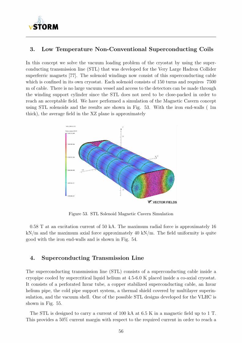
3. Low Temperature Non-Conventional Superconducting Coils

In this concept we solve the vacuum loading problem of the cryostat by using the super-

conducting transmission line (STL) that was developed for the Very Large Hadron Collider

superferric magnets [77]. The solenoid windings now consist of this superconducting cable

which is confined in its own cryostat. Each solenoid consists of 150 turns and requires 7500

m of cable. There is no large vacuum vessel and access to the detectors can be made through

the winding support cylinder since the STL does not need to be close-packed in order to

reach an acceptable field. We have performed a simulation of the Magnetic Cavern concept

using STL solenoids and the results are shown in Fig. 53. With the iron end-walls ( 1m

thick), the average field in the XZ plane is approximately

Figure 53. STL Solenoid Magnetic Cavern Simulation

0.58 T at an excitation current of 50 kA. The maximum radial force is approximately 16

kN/m and the maximum axial force approximately 40 kN/m. The field uniformity is quite

good with the iron end-walls and is shown in Fig. 54.

4. Superconducting Transmission Line

The superconducting transmission line (STL) consists of a superconducting cable inside a

cryopipe cooled by supercritical liquid helium at 4.5-6.0 K placed inside a co-axial cryostat.

It consists of a perforated Invar tube, a copper stabilized superconducting cable, an Invar

helium pipe, the cold pipe support system, a thermal shield covered by multilayer superin-

sulation, and the vacuum shell. One of the possible STL designs developed for the VLHC is

shown in Fig. 55.

The STL is designed to carry a current of 100 kA at 6.5 K in a magnetic field up to 1 T.

This provides a 50% current margin with respect to the required current in order to reach a

56

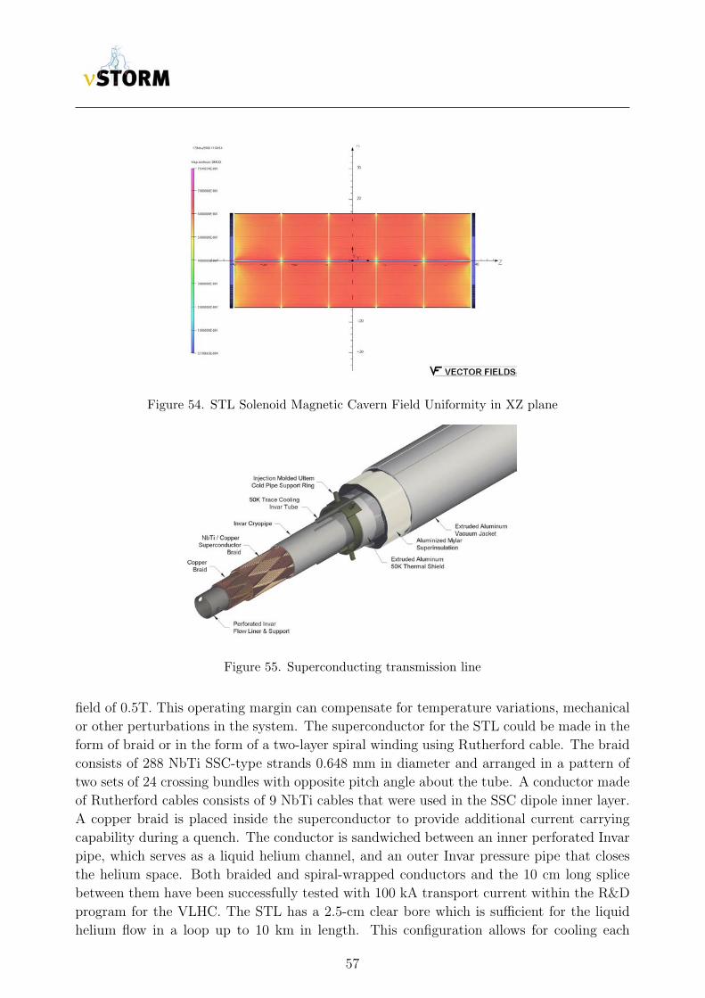
Figure 54. STL Solenoid Magnetic Cavern Field Uniformity in XZ plane

Figure 55. Superconducting transmission line

field of 0.5T. This operating margin can compensate for temperature variations, mechanical

or other perturbations in the system. The superconductor for the STL could be made in the

form of braid or in the form of a two-layer spiral winding using Rutherford cable. The braid

consists of 288 NbTi SSC-type strands 0.648 mm in diameter and arranged in a pattern of

two sets of 24 crossing bundles with opposite pitch angle about the tube. A conductor made

of Rutherford cables consists of 9 NbTi cables that were used in the SSC dipole inner layer.

A copper braid is placed inside the superconductor to provide additional current carrying

capability during a quench. The conductor is sandwiched between an inner perforated Invar

pipe, which serves as a liquid helium channel, and an outer Invar pressure pipe that closes

the helium space. Both braided and spiral-wrapped conductors and the 10 cm long splice

between them have been successfully tested with 100 kA transport current within the R&D

program for the VLHC. The STL has a 2.5-cm clear bore which is sufficient for the liquid

helium flow in a loop up to 10 km in length. This configuration allows for cooling each

57

solenoid with continuous helium flow coming from a helium distribution box.

The thermal shield is made of extruded aluminum pipe segments, which slide over opposite

ends of each support spider. The 6.4-mm diameter Invar pipe is used for 50 K pressurized

helium. It is placed in the cavities at the top and the bottom of both the shield and the

supports. The shield is wrapped with 40 layers of a dimpled super insulation. The vacuum

shell is made of extruded aluminum or stainless steel. Heat load estimates for the described

STL are:

• Support system: 53 mW/m at 4.5 K and 670 mW/m at 40 K

• Super insulation: 15 mW/m at 4.5 K and 864 mW/m at 40K

The estimated cost of the described STL is approximately $500/m. Further STL design

optimization will be required to adjust the structure to the fabrication and operating condi-

tions of the desired detector solenoids and to optimize its fabrication and operational cost.

5. Conclusions

Magnetizing volumes large enough to contain upwards of 1kT of LAr or totally active scin-

tillator at fields up to 0.5T with the use of the STL concept would appear to be possible, but

would require dedicated R&D to extend the STL developed for the VLHC to this applica-

tion. It eliminates the cost driver of large conventional superconducting coils, the vacuum-

insulated cryostat, and has already been prototyped, tested, and costed during the R&D for

the VLHC. A full engineering design would still need to be done, but this technique has the

potential to deliver the large magnetic volume required with a field as high as 1T, with very

uniform field quality and at an acceptable cost.

58

[1] D. G. Koshkarev, “Proposal for a Decay Ring to Produce Intense Secondary Particle Beams

at the SPS,” (1974), CERN/ISR-DI/74-62.

[2] D. Neuffer, “Design Considerations for a Muon Storage Ring,” (1980), Telmark Conference

on Neutrino Mass, Barger and Cline eds., Telmark, Wisconsin.

[3] S. Geer, Phys.Rev. D57, 6989 (1998), arXiv:hep-ph/9712290 [hep-ph].

[4] S. Choubey et al. (The IDS-NF collaboration), (2011), arXiv:1112.2853 [hep-ex].

[5] K. Abazajian, M. Acero, S. Agarwalla, A. Aguilar-Arevalo, C. Albright, et al., (2012),

arXiv:1204.5379 [hep-ph].

[6] M. Bando and K. Yoshioka, Prog.Theor.Phys. 100, 1239 (1998), arXiv:hep-ph/9806400 [hep-

ph].

[7] E. Ma, Phys.Lett. B380, 286 (1996), arXiv:hep-ph/9507348 [hep-ph].

[8] Q. Shafi and Z. Tavartkiladze, Phys.Lett. B451, 129 (1999), arXiv:hep-ph/9901243 [hep-ph].

[9] K. Babu and G. Seidl, Phys.Rev. D70, 113014 (2004), arXiv:hep-ph/0405197 [hep-ph].

[10] A. Kusenko, F. Takahashi, and T. T. Yanagida, Phys.Lett. B693, 144 (2010),

arXiv:1006.1731 [hep-ph].

[11] R. Mohapatra, Phys.Rev. D64, 091301 (2001), arXiv:hep-ph/0107264 [hep-ph].

[12] C. Froggatt and H. B. Nielsen, Nucl.Phys. B147, 277 (1979).

[13] J. Barry, W. Rodejohann, and H. Zhang, JCAP 1201, 052 (2012), arXiv:1110.6382 [hep-ph].

[14] R. Mohapatra, S. Nasri, and H.-B. Yu, Phys.Rev.D72, 033007 (2005), arXiv:hep-ph/0505021

[hep-ph].

[15] C. S. Fong, R. N. Mohapatra, and I. Sung, Phys.Lett. B704, 171 (2011), arXiv:1107.4086

[hep-ph].

[16] H. Zhang, (2011), arXiv:1110.6838 [hep-ph].

[17] Z. G. Berezhiani and R. N. Mohapatra, Phys.Rev. D52, 6607 (1995), arXiv:hep-ph/9505385

[hep-ph].

[18] R. Foot and R. Volkas, Phys.Rev. D52, 6595 (1995), arXiv:hep-ph/9505359 [hep-ph].

[19] V. Berezinsky, M. Narayan, and F. Vissani, Nucl.Phys. B658, 254 (2003), arXiv:hep-

ph/0210204 [hep-ph].

[20] A. Aguilar et al. (LSND), Phys. Rev. D64, 112007 (2001), arXiv:hep-ex/0104049.

[21] A. Aguilar-Arevalo et al. (The MiniBooNE Collaboration), Phys.Rev.Lett. 98, 231801 (2007),

arXiv:0704.1500 [hep-ex].

[22] A. Aguilar-Arevalo et al. (The MiniBooNE Collaboration), Phys.Rev.Lett. 105, 181801

(2010), arXiv:1007.1150 [hep-ex].

[23] T. Mueller, D. Lhuillier, M. Fallot, A. Letourneau, S. Cormon, et al., Phys.Rev. C83, 054615

(2011), arXiv:1101.2663 [hep-ex].

[24] K. Schreckenbach, G. Colvin, W. Gelletly, and F. Von Feilitzsch, Phys.Lett. B160, 325

(1985).

[25] P. Huber, Phys.Rev. C84, 024617 (2011), arXiv:1106.0687 [hep-ph].

59

[26] G. Mention, M. Fechner, T. Lasserre, T. Mueller, D. Lhuillier, et al., Phys.Rev. D83, 073006

(2011), arXiv:1101.2755 [hep-ex].

[27] P. Anselmann et al. (GALLEX Collaboration.), Phys.Lett. B342, 440 (1995).

[28] W. Hampel et al. (GALLEX Collaboration), Phys.Lett. B420, 114 (1998).

[29] J. Abdurashitov, V. Gavrin, S. Girin, V. Gorbachev, T. V. Ibragimova, et al., Phys.Rev.Lett.

77, 4708 (1996).

[30] J. Abdurashitov et al. (SAGE Collaboration), Phys.Rev. C59, 2246 (1999), arXiv:hep-

ph/9803418 [hep-ph].

[31] J. Abdurashitov, V. Gavrin, S. Girin, V. Gorbachev, P. Gurkina, et al., .

[32] M. A. Acero, C. Giunti, and M. Laveder, Phys.Rev. D78, 073009 (2008), arXiv:0711.4222

[hep-ph].

[33] C. Giunti and M. Laveder, Phys.Rev. D82, 053005 (2010), arXiv:1005.4599 [hep-ph].

[34] C. Giunti and M. Laveder, Phys.Rev. C83, 065504 (2011), arXiv:1006.3244 [hep-ph].

[35] J. Kopp, M. Maltoni, and T. Schwetz, Phys.Rev.Lett. 107, 091801 (2011), arXiv:1103.4570

[hep-ph].

[36] C. Giunti and M. Laveder, Phys.Lett. B706, 200 (2011), arXiv:1111.1069 [hep-ph].

[37] G. Karagiorgi, (2011), arXiv:1110.3735 [hep-ph].

[38] C. Giunti and M. Laveder, Phys.Rev. D84, 093006 (2011), arXiv:1109.4033 [hep-ph].

[39] C. Giunti and M. Laveder, Phys.Rev. D84, 073008 (2011), arXiv:1107.1452 [hep-ph].

[40] B. Armbruster et al. (KARMEN), Phys. Rev. D65, 112001 (2002), arXiv:hep-ex/0203021.

[41] P. Astier et al. (NOMAD), Nucl. Phys. B611, 3 (2001), arXiv:hep-ex/0106102.

[42] F. Dydak, G. Feldman, C. Guyot, J. Merlo, H. Meyer, et al., Phys.Lett. B134, 281 (1984).

[43] Y. Ashie et al. (Super-Kamiokande), Phys. Rev. D71, 112005 (2005), hep-ex/0501064.

[44] P. Adamson et al. (The MINOS Collaboration), Phys.Rev. D81, 052004 (2010),

arXiv:1001.0336 [hep-ex].

[45] P. Adamson et al. (MINOS Collaboration), Phys.Rev.Lett. 107, 011892 (2011),

arXiv:1104.3922 [hep-ex].

[46] Y. Declais, J. Favier, A. Metref, H. Pessard, B. Achkar, et al., Nucl.Phys. B434, 503 (1995).

[47] Y. Declais, H. de Kerret, B. Lefievre, M. Obolensky, A. Etenko, et al., Phys.Lett. B338, 383

(1994).

[48] A. Kuvshinnikov, L. Mikaelyan, S. Nikolaev, M. Skorokhvatov, and A. Etenko, JETP Lett.

54, 253 (1991).

[49] G. Vidyakin, V. Vyrodov, I. Gurevich, Y. Kozlov, V. Martemyanov, et al., Sov.Phys.JETP

66, 243 (1987).

[50] H. Kwon, F. Boehm, A. Hahn, H. Henrikson, J. Vuilleumier, et al., Phys.Rev. D24, 1097

(1981).

[51] G. Zacek et al. (CALTECH-SIN-TUM), Phys. Rev. D34, 2621 (1986).

[52] M. Apollonio et al. (CHOOZ), Eur. Phys. J. C27, 331 (2003), arXiv:hep-ex/0301017.

[53] F. Boehm, J. Busenitz, B. Cook, G. Gratta, H. Henrikson, et al., Phys.Rev. D64, 112001

(2001), arXiv:hep-ex/0107009 [hep-ex].

60

[54] P. Huber, M. Lindner, and W. Winter, Comput. Phys. Commun. 167, 195 (2005), arXiv:hep-

ph/0407333.

[55] P. Huber, J. Kopp, M. Lindner, M. Rolinec, and W. Winter, Comput. Phys. Commun. 177,

432 (2007), hep-ph/0701187.

[56] M. C. Gonzalez-Garcia and M. Maltoni, Phys. Rept. 460, 1 (2008), arXiv:0704.1800 [hep-ph].

[57] M. Maltoni and T. Schwetz, Phys. Rev. D76, 093005 (2007), arXiv:0705.0107 [hep-ph].

[58] E. Akhmedov and T. Schwetz, JHEP 10, 115 (2010), arXiv:1007.4171 [hep-ph].

[59] M. Maltoni and T. Schwetz, Phys. Rev. D68, 033020 (2003), arXiv:hep-ph/0304176.

[60] M. Gonzalez-Garcia, M. Maltoni, and J. Salvado, JHEP 08, 117 (2010), arXiv:1006.3795

[hep-ph].

[61] J. Hamann, S. Hannestad, G. G. Raffelt, I. Tamborra, and Y. Y. Wong, Phys.Rev.Lett. 105,

181301 (2010), arXiv:1006.5276 [hep-ph].

[62] E. Giusarma, M. Corsi, M. Archidiacono, R. de Putter, A. Melchiorri, et al., Phys.Rev. D83,

115023 (2011), arXiv:1102.4774 [astro-ph.CO].

[63] G. Mangano and P. D. Serpico, Phys.Lett. B701, 296 (2011), arXiv:1103.1261 [astro-ph.CO].

[64] J. Hamann, S. Hannestad, G. G. Raffelt, and Y. Y. Wong, JCAP 1109, 034 (2011),

arXiv:1108.4136 [astro-ph.CO].

[65] L. Bento and Z. Berezhiani, Phys.Rev. D64, 115015 (2001), arXiv:hep-ph/0108064 [hep-ph].

[66] A. Dolgov and F. Takahashi, Nucl.Phys. B688, 189 (2004), arXiv:hep-ph/0402066 [hep-ph].

[67] G. Karagiorgi, M. Shaevitz, and J. Conrad, (2012), arXiv:1202.1024 [hep-ph].

[68] J. Hewett, H. Weerts, R. Brock, J. Butler, B. Casey, et al., (2012), arXiv:1205.2671 [hep-ex].

[69] P. Huber, M. Mezzetto, and T. Schwetz, JHEP 0803, 021 (2008), arXiv:0711.2950 [hep-ph].

[70] P. Coloma, A. Donini, E. Fernandez-Martinez, and P. Hernandez, (2012), 30 pages, 9 figures,

arXiv:1203.5651 [hep-ph].

[71] J. Formaggio and G. Zeller, “From eV to EeV: Neutrino Cross Sections Across Energy Scales,”

(2012), to be published in Rev. Mod. Phys.

[72] D. Casper, Nucl.Phys.Proc.Suppl. 112, 161 (2002), to be published in Proceedings of the

First International Workshop on Neutrino-Nucleus Interactions in the Few-GeV Region

(NUINT’01), arXiv:hep-ph/0208030 [hep-ph].

[73] N. Mokhov, J.Nucl.Sci.Tech. S1, 167 (2000).

[74] N. Bozhko et al., Yad. Fiz 31, 1494.

[75] L. Barkov et al., Sov. J. Nucl. Phys. 35(5), 694.

[76] D. G. Michael et al. (MINOS), Nucl. Instrum. Meth. A596, 190 (2008), arXiv:0805.3170

[physics.ins-det].

[77] G. Ambrosio et al. (VLHC Design Study Group), (2001).

[78] R. Smith et al. (USCMS Collaboration), IEEE Trans.Appl.Supercond. 14, 1830 (2004).

[79] H. Maesaka (K2K SciBar Collaboration), , 185 (2003).

[80] Y. Kudenko (T2K), Nucl. Instrum. Meth. A598, 289 (2009), arXiv:0805.0411 [physics.ins-

det].

[81] D. Greiner, T. Lachenmaier, J. Jochum, and A. Cabrera, Nucl. Instrum. Meth. A581, 139

(2007).

61

[82] Z. Sadygov, (1996), russian patent No. 2102820.

[83] N. Bacchetta et al., Nucl. Instrum. Meth. A383, 263 (1996).

[84] D. Renker, Nucl.Instrum.Meth. A598, 207 (2009).

[85] B. Dolgoshein (SIPM Collaboration), , 442 (2003).

[86] K. Bechtol, S. Funk, A. Okumura, L. Ruckman, A. Simons, et al., submitted to Nuclear

Instrumentation and Methods (NIM) (2011), arXiv:1105.1832 [astro-ph.IM].

[87] S. R. Mishra, Prog.Part.Nucl.Phys. 64, 202 (2010).

[88] J. Altegoer et al. (NOMAD Collaboration), Nucl.Instrum.Meth. A404, 96 (1998).

[89] T. Akesson et al. (ATLAS TRT Collaboration), Nucl.Instrum.Meth. A522, 131 (2004).

[90] V. Bychkov, M. Faessler, R. Geyer, N. Gorbacheva, Y. Gusakov, et al., Part.Nucl.Lett. 111,

64 (2002).

[91] C. Andreopoulos et al., Nucl. Instrum. Meth. A614, 87 (2010), arXiv:0905.2517 [hep-ph].

[92] J. Apostolakis and D. H. Wright (Geant4), AIP Conf. Proc. 896, 1 (2007).

[93] “Geant4 Physics Reference Manual,” http://geant4.cern.ch/geant4/UserDocumentation/UsersGuides/

PhysicsReferenceManual/html/.

[94] A. Pla-Dalmau, A. D. Bross, V. V. Rykalin, and B. M. Wood (MINERvA), “Extruded plastic

scintillator for MINERvA,” (2005), proceedings of 2005 IEEE Nuclear Science Symposium

and Medical Imaging Conference, El Conquistador Resort, Puerto Rico, 23-29 Oct 2005.

[95] A. Cervera, A. Laing, J. Martin-Albo, and F. J. P. Soler, Nucl. Instrum. Meth. A624, 601

(2010), arXiv:1004.0358 [hep-ex].

[96] A. Laing, PhD thesis, University of Glasgow (2010).

[97] A. Cervera-Villanueva, J. J. Gomez-Cadenas, and J. A. Hernando, Nucl. Instrum. Meth.

A534, 180 (2004).

[98] D. Emeliyanov, I. Gorbounov, and I. Kisel, “OTR/ITR-CATS: Tracking Based on Cellular

Automaton and Kalman Filter,” (2001), HERA-B note 01-137.

[99] D. Groom, N. Mokhov, and S. Striganov, Atomic Data and Nuclear Data Tables 78, 183

(2001).

[100] P. Adamson et al., Nucl. Instrum. Meth. A556, 119 (2006).

[101] G. Bari et al., Nucl. Instrum. Meth. A508, 170 (2003).

[102] A. Blondel, M. Campanelli, and M. Fechner, Nucl. Instrum. Meth. A535, 665 (2004).

[103] C. D. Tunnell, J. H. Cobb, and A. D. Bross, (2011), arXiv:1111.6550 [hep-ph].

[104] C. Tunnell, (2012), arXiv:1205.6338 [hep-ph].

[105] W. Winter, (2012), arXiv:1204.2671 [hep-ph].

[106] H. Minakata, H. Sugiyama, O. Yasuda, K. Inoue, and F. Suekane, Phys.Rev. D70, 059901

(2004), arXiv:hep-ph/0211111 [hep-ph].

[107] P. Huber, M. Lindner, T. Schwetz, and W. Winter, Nucl.Phys. B665, 487 (2003), arXiv:hep-

ph/0303232 [hep-ph].

[108] C. Giunti, M. Laveder, and W. Winter, Phys.Rev. D80, 073005 (2009), arXiv:0907.5487

[hep-ph].

[109] J. Tang and W. Winter, Phys.Rev. D80, 053001 (2009), arXiv:0903.3039 [hep-ph].

62

[110] T. Abe et al. (ISS Detector Working Group), JINST 4, T05001 (2009), detector report of the

International Scoping Study of a future Neutrino Factory and Super-Beam facility, 86 pages,

49 figures, arXiv:0712.4129 [physics.ins-det].

[111] M. Green, “Private communication,”.

[112] M. Green and S. St. Lorant, Adv.Cryog.Eng. 39A, 271 (1994).

[113] A. Herve, G. Acquistapace, D. Campi, P. Cannarsa, P. Fabbricatore, et al., IEEE

Trans.Appl.Supercond. 12, 385 (2002).

[114] V. Balbekov, “MuCool Note 216,” (2001).

63