Seminar, 4. year

Neutrinoless double beta decay

Author: Blaz LebanFaculty of Mathematics and Physics, University of Ljubljana

Advisor: doc. dr. Miha NemevsekJozef Stefan Institute, Ljubljana

Ljubljana, February 2017

Abstract

Firstly, we focus on some basic properties of spinor manipulation and derive two Lagrangiansin different representations. We also present the role of neutrinos in three different kinds of betadecays, the most important of them being neutrinoless double beta decay. We briefly calculate itsamplitude and in the end, we describe an experimental collaboration GERDA which is in searchfor Neutrinoless double beta decay and is currently lowering the upper neutrino mass limit.

Contents

1 Introduction 1

2 Lorentz Invariance 12.1 Chiral (Weyl) representation . . . . . . . . . . . . . . . . . . . . . . . . . . . . . . . . 2

3 Dirac spinors 2

4 Majorana spinors 34.1 Particles and antiparticles . . . . . . . . . . . . . . . . . . . . . . . . . . . . . . . . . . 4

5 Neutrinos and beta decay 55.1 Double beta decay (2ν2β) . . . . . . . . . . . . . . . . . . . . . . . . . . . . . . . . . . 55.2 Neutrinoless double beta decay (0ν2β) . . . . . . . . . . . . . . . . . . . . . . . . . . . 55.3 Where do neutrino masses come from? . . . . . . . . . . . . . . . . . . . . . . . . . . . 75.4 Amplitude for neutrinoless double beta decay . . . . . . . . . . . . . . . . . . . . . . . 7

6 GERDA experiment 86.1 Results . . . . . . . . . . . . . . . . . . . . . . . . . . . . . . . . . . . . . . . . . . . . . 8

7 Conclusions 9

1 Introduction

Standard Model by itself does not allow neutrinos to have mass, but from the latest experimental datawe know, that they are in fact not massless. Thus, Standard Model must not be considered as thedefinite and final theory and some corrections have to be made. It was in 1937, when E. Majoranapublished a paper, in which he proposed a theory, where a particle (Majorana type) can be identicalto its own antiparticle. If the neutrino is a Majorana particle and at least one type of neutrino hasnon-zero mass, then it is possible for Neutrinoless Double Beta Decay (0ν2β) to occur. Observing thiskind of process, in addition to confirming the Majorana neutrino nature, would give information onthe absolute neutrino mass scale, potentially the neutrino mass hierarchy and Majorana phases in thePMNS matrix. Due to all these important not yet known informations about neutrino physics, manyexperiments are trying to detect 0ν2β process in large and very sensitive detectors.

2 Lorentz Invariance

When we say that an equation is Lorentz invariant, we actually mean, that it holds in any referenceframe. So, if one function (e.g. scalar field φ) satisfies a certain equation in one frame and thenwe perform any boost or rotation to another frame of reference, the function must satisfy the sameequation in this new frame. We can write an arbitrary Lorentz transformation as

xµ → x′µ = Λµν xν and for the field Φ(x)→ Φ′(x) = Φ(Λ−1x), (2.1)

where Λ is some 4× 4 matrix. In turns out that most general non-linear transformations can be builtfrom linear transformations, so the Lorentz invariance law can simply be written as

Φ→M(Λ)Φ, (2.2)

where matrices M form a n-dimensional Lorentz group. General representation of M matrices is then

M = exp

(− i

2

∑µν

ωµνJµν

), (2.3)

where J-s are generators of this Lorentz group and depend on spin (J = J(s)) and ωµν depend ondesired transformation Λ, which is the same for all spins.

1

Lorentz invariance is especially simple to prove, if we start from the Lagrangian formulation of thefield theory. It turns out, that any equation of motion, which is derived from the Lagrangian, whichis a Lorentz scalar 1, is automatically Lorentz invariant [1].

2.1 Chiral (Weyl) representation

It is convenient for us now to choose the chiral representation of gamma matrices, so that we can formtwo 2-dimensional representations and write

ψ =

(ψLψR

). (2.4)

The two component objects ψL and ψR are called left-handed and right-handed Weyl spinors. Thegamma matrices are then

γµ =

(0 σµ

σµ 0

), (2.5)

where σµ = (1, σi) and σµ = (1,−σi) [1].Rotation and boost generators can be in general constructed by Σµν matrices, where

Σµν =1

2σµν =

i

4[γµ, γν ]. (2.6)

In general the boost and rotation transformation can be then written as

ψ → Λψ = exp(iΣµνθµν

)ψ = ei

~θ2(~σ+i~ϕ)ψ, (2.7)

where θ0i = ~ϕ represent boosts and ~θi = εijkθjk rotations.

3 Dirac spinors

Let us denote a four component Dirac spinor by ψD. The Dirac Lagrangian density is then

LDIRAC = ψD(i/∂ −m

)ψD, (3.1)

where we used natural units ~ = c = 1. From this we can easily get the Dirac equation from Euler -Lagrange equation:

∂LD∂(∂µψD)

− ∂LD∂ψD

= 0 =⇒ (i/∂ −m)ψD = 0. (3.2)

Let us check if this Dirac Lagrangian LD is Lorentz invariant. We will transform it term by term:

Kinetic: iψD /∂ψD → iψDΛ−1γµΛ∂µψD = iψDΛµνγν∂µψD = iψDγ

µ∂µψD,

Mass: mψDψD → mψD Λ−1Λ︸ ︷︷ ︸I

ψD. (3.3)

We can see that the equation stays the same, so the Dirac Lagrangian is Lorentz invariant.It is often useful to work with Weyl spinors χ instead of this Dirac 4-component representation. Wedefine some useful relations:

PR,L =1

2(1± γ5), so ψL = PLψD =

(χL0

), and ψR = PRψD =

(0χR

). (3.4)

Lorentz transformation stays the same as in Eq.(2.7), so:

χL,R −→ exp

[i~σ

2(~θ ± i~ϕ)

]χL,R. (3.5)

1A Lorentz scalar is a scalar which is invariant under a Lorentz transformation. It can be generated from multiplicationof vectors or tensors, even if the components of these are not Lorentz invariant.

2

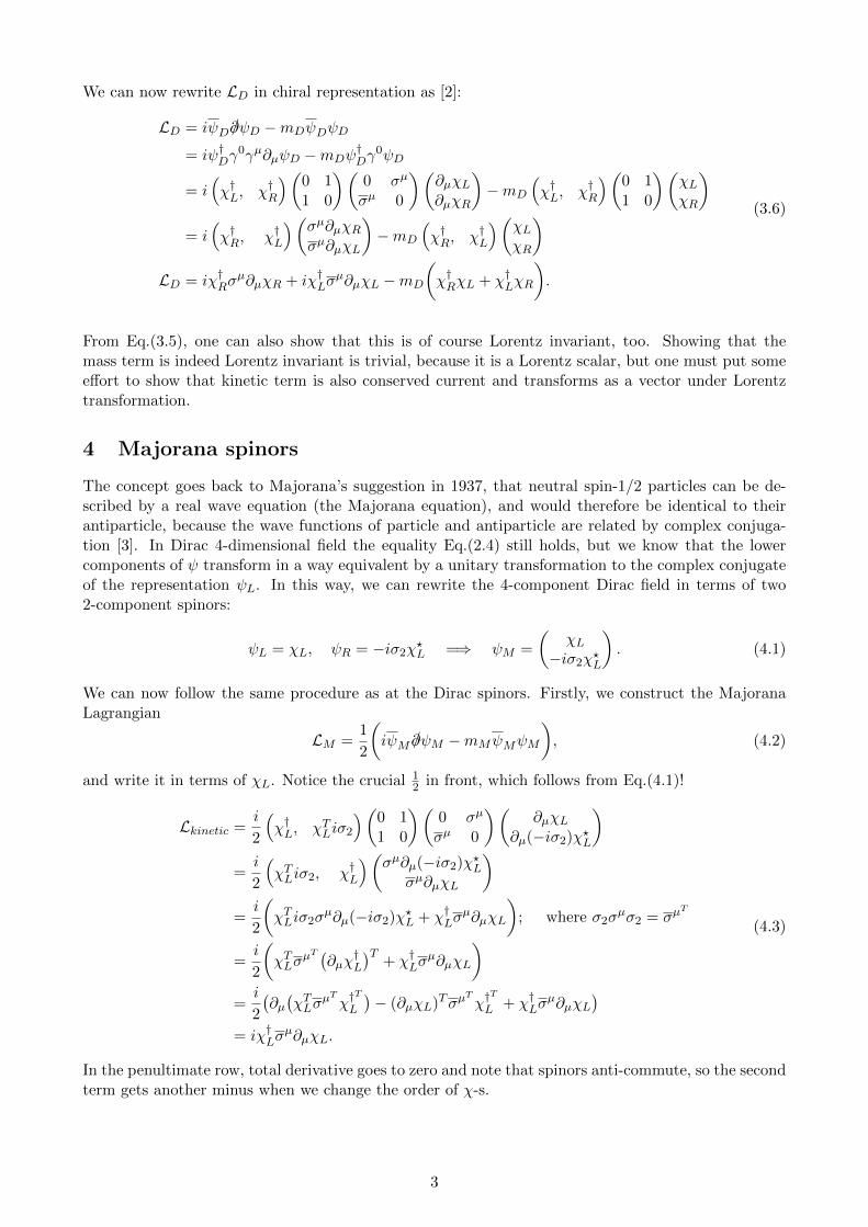
We can now rewrite LD in chiral representation as [2]:

LD = iψD /∂ψD −mDψDψD

= iψ†Dγ0γµ∂µψD −mDψ

†Dγ

0ψD

= i(χ†L, χ†R

)(0 11 0

)(0 σµ

σµ 0

)(∂µχL∂µχR

)−mD

(χ†L, χ†R

)(0 11 0

)(χLχR

)= i(χ†R, χ†L

)(σµ∂µχRσµ∂µχL

)−mD

(χ†R, χ†L

)(χLχR

)LD = iχ†Rσ

µ∂µχR + iχ†Lσµ∂µχL −mD

(χ†RχL + χ†LχR

).

(3.6)

From Eq.(3.5), one can also show that this is of course Lorentz invariant, too. Showing that themass term is indeed Lorentz invariant is trivial, because it is a Lorentz scalar, but one must put someeffort to show that kinetic term is also conserved current and transforms as a vector under Lorentztransformation.

4 Majorana spinors

The concept goes back to Majorana’s suggestion in 1937, that neutral spin-1/2 particles can be de-scribed by a real wave equation (the Majorana equation), and would therefore be identical to theirantiparticle, because the wave functions of particle and antiparticle are related by complex conjuga-tion [3]. In Dirac 4-dimensional field the equality Eq.(2.4) still holds, but we know that the lowercomponents of ψ transform in a way equivalent by a unitary transformation to the complex conjugateof the representation ψL. In this way, we can rewrite the 4-component Dirac field in terms of two2-component spinors:

ψL = χL, ψR = −iσ2χ?L =⇒ ψM =

(χL

−iσ2χ?L

). (4.1)

We can now follow the same procedure as at the Dirac spinors. Firstly, we construct the MajoranaLagrangian

LM =1

2

(iψM /∂ψM −mMψMψM

), (4.2)

and write it in terms of χL. Notice the crucial 12 in front, which follows from Eq.(4.1)!

Lkinetic =i

2

(χ†L, χTLiσ2

)(0 11 0

)(0 σµ

σµ 0

)(∂µχL

∂µ(−iσ2)χ?L

)=i

2

(χTLiσ2, χ†L

)(σµ∂µ(−iσ2)χ?Lσµ∂µχL

)=i

2

(χTLiσ2σ

µ∂µ(−iσ2)χ?L + χ†Lσµ∂µχL

); where σ2σ

µσ2 = σµT

=i

2

(χTLσ

µT(∂µχ

†L

)T+ χ†Lσ

µ∂µχL

)=i

2

(∂µ(χTLσ

µTχ†T

L

)− (∂µχL)Tσµ

Tχ†

T

L + χ†Lσµ∂µχL

)= iχ†Lσ

µ∂µχL.

(4.3)

In the penultimate row, total derivative goes to zero and note that spinors anti-commute, so the secondterm gets another minus when we change the order of χ-s.

3

Lmass = −m2

(χ†L, χTLiσ2

)(0 11 0

)(χL

−iσ2χ?L

)= −m

2

(χ†L, χTLiσ2

)(−iσ2χ?LχL

)= −m

2

(− χ†Liσ2χ

?L + χTLiσ2χL

).

(4.4)

When we put this two terms together, we get the full Majorana Lagrangian density, which is slightlydifferent from the Dirac one, but it is still Lorentz invariant [2].

LM = iχ†L/∂χL −1

2m

(χTLiσ2χL + h.c.

). (4.5)

4.1 Particles and antiparticles

In quantum electrodynamics the Dirac Lagrangian is

LQED = −1

4FµνFµν + ψD

(i /D −m

)ψD, (4.6)

from where we get conserved current jµ = ψDγµψD. Charge is defined as the integral of the zeroth

component of this current as

Q = e0

∫VψDγ

0ψD dV. (4.7)

Let us now define a charge conjugation operator

C = iγ2γ0, CT = −C, C2 = 1, (4.8)

and see how it affects Dirac and Majorana spinors.

ψCD = CψT

= iγ2γ0(ψ†γ0)

T = iγ2ψ? =

(0 iσ2−iσ2 0

)(χ?Lχ?R

)=

(iσ2χ

?R

−iσ2χ?L

). (4.9)

Since there is a conjugation of the spinor on the very right hand side, one can show that Q(ψD) =−Q(ψCD). This means that the antiparticles have the opposite charge from particles. Furthermore, wecan show the following relation:

ψM = PLψD + PRψCD =

(χL0

)+

(0

−iσ2χ?L

)=

(χL

−iσ2χ?L

). (4.10)

The Majorana spinor is therefore composed of a left-handed particle and right-handed antiparticle.And what happens with the Majorana spinor under the charge conjugation?

ψCM = iγ2ψ?M =

(0 iσ2−iσ2 0

)(χ?L

iσ?2χL

)=

(χL

−iσ2χ?L

)= ψM . (4.11)

The charge conjugated Majorana spinor is equal to itself, so the particles and antiparticles have equalcharge (and equal mass) and they are identical in Majorana picture as we have already mentioned.Since there is a mass term in the Majorana Lagrangian we can not define any U(1) charge to theMajorana spinor, because the associated current is explicitly equal to zero.

4

5 Neutrinos and beta decay

It is because of neutrinos, that the electron spectrum of beta decay is continuous. But since we knowthat neutrinos are not massless, few experiments are searching for distortion in the close to end-pointspectrum of beta decay, because if neutrinos have mass, the maximal electron energy is Q − mν .This fact is depicted in Fig. (1a) for a massless (dotted) and two different massive (continuous line)neutrinos.

Figure 1: Beta decay spectrum. Reproduced from [4].

(a) β-decay spectrum close to end-point. (b) 2ν2β and 0ν2β spectrum.

5.1 Double beta decay (2ν2β)

Some nuclei can only decay trough double beta decay, which was proposed by Maria Goeppert Mayerin 1935. This means that two neutrons simultaneously change into two protons, two electrons andtwo anti-neutrinos

n→ p e− νe. (5.1)

This is due to the fact, that some even-even nuclei (A,Z) can not β-decay into another nuclei with(A,Z + 1), because the latter is heavier. So the only possible channel is to decay into

(A,Z) −→ (A,Z + 2) + 2e− + 2 νe. (5.2)

Figure 2: Single beta decay isforbidden [5].

One example is 7632Ge that can not decay into 76

33As. It can only jumpinto 76

34Se:

7632Ge −→ 76

34Se + 2 e− + 2 νe, (Q = 2038, 6 keV). (5.3)

Since this process involves the weak force twice, the process is veryrare, but still observable. With a half-life on the order of 10 billiontimes the age of the Universe (which is 14 billion years old), it hasbeen seen in a number of even-even nuclei. We can see the doublebeta decay spectrum in Fig. (1b) and its Feynman diagram in Fig.(3a).

5.2 Neutrinoless double beta decay (0ν2β)

If neutrinos are Majorana particles, another process would be possible. It is called NeutrinolessDouble Beta Decay and was proposed by G. Racah and W. H. Furry in 1937 [6, 7]. The only quantumnumber that can be used to distinguish between neutrino and anti-neutrino states is lepton numberL. However, there is no gauge symmetry associated with lepton number and there is no fundamentalreason this quantity should be conserved. If lepton number is violated, the distinction between νand ν is unclear and it becomes possible that neutrinos can be their own anti-particles or so calledMajorana fermions. Determining the nature of neutrinos is difficult, but a promising approach is tosearch for the 0ν2β of an atomic nucleus [8]. In Germanium case it looks like:

7632Ge −→ 76

34Se + e− + e−. (5.4)

5

(a) 2ν2β process. (b) 0ν2β process.

Figure 3: Feynman diagrams for double beta decay. On the right hand side (0ν2β) the two neutrinosannihilate and the lepton number is not conserved.

This process violates the lepton number conservation by two units (∆L = 2), but its observation issufficient to show that the neutrino is a Majorana fermion. Since neutrinos annihilate, the total energyof the two outcoming electrons is equal to Q, so the expected spectrum is a delta function at Q, asseen in Fig. (1b). Feynman diagram for this process is seen on Fig. (3b).We know that neutrinos oscillate, but this process depends only on the difference between squaresof neutrino masses, so from the experimental data, we can only get, e.g. ∆m2

ij = m2j − m2

i , wherei, j ∈ 1, 2, 3 but not the individual masses that will parametrize the decay rate of the process. Wehave already determined the ∆m2

12 = (7.5±0.2)×105 eV2 and |∆m223| = (2.5±0.2)×10−3 eV2 (taken

from [9]), but we do not know the sign of the latter, so we must consider two different situations calledNormal hierarchy (m2

1 < m22 < m2

3) and Inverted hierarchy (m23 < m2

1 < m22), seen on Fig. (4a).

On the other hand, neutrinoless double beta decay experiments measure the 0ν2β decay rate Γ0ν2β

which is actually proportional to the absolute value squared of the last column of UPMNS (neutrinomixing matrix):

|mee| = |∑i

U2eiνi| = | cos2 θ13(ν1e

2iβ cos2 θ12 + ν2e2iα sin2 θ12) + ν3 sin2 θ13|. (5.5)

Now, we can plot a graph and see the dependence of |mee| on lightest neutrino mass.

Figure 4

(a) Normal hierarchy: ∆m223 > 0 and inverted one

∆m223 < 0. Adapted from [10].

(b) Expected ranges as function of the lightest neu-trino mass. Figure was made by my Python script.

6

5.3 Where do neutrino masses come from?

In the Standard Model, the SU(2)L × U(1)Y gauge symmetry prevents us from simply writing downthe Majorana mass term. We can either consider non-renormalizable terms or add new particles,which may contribute to the 0ν2β rate as well. For simplicity, we introduce a non-renormalizableLagrangian called dimension 5 Weinberg operator:

Ld=5 = −yM (LT iτ2H)iσ2(HT iτ2L)

M+ h.c., where L =

(νe

), (5.6)

and iτ2 makes the (LT iτ2H) term gauge invariant (τi are just Pauli matrices) and iσ2 Lorentz invariant.L is the left-handed lepton doublet [11]. When the Higgs doublet gets a non vanishing vacuumexpectation value (vev),

〈H〉 =

(0v√2

), v = 246 GeV, (5.7)

neutrino gets the Majorana mass. If we further compute Weinberg operator using L and 〈H〉, we get

Ld=5 = yMv2

2MνT iσ2ν + h.c.

Comparing this result with Eq.(4.5), we can compute neutrino mass as

mν := yMv2

M. (5.8)

We can also recognize this masses as the components of the UPMNS . From here on, we only need the

ratio of yM

M , where the new scale M signifies some new physics. We do not know neither yM nor M ,but fortunately, we can connect it with the 0ν2β. We will do this in next section.

5.4 Amplitude for neutrinoless double beta decay

For neutrinoless double beta decay we write the ordinary weak interaction Lagrangian [11]

Lint =g

2√

2

(ueγ

µ 1

2(1− γ5)uνM − uνMγ

µ 1

2(1 + γ5)uce

)W−µ + h.c. (5.9)

Notice that we used PL in the left part and PR in the right. If we then write the amplitude for theprocess from this Lagrangian, we multiply both these parts.

M∝(ueγ

µPLuνM)(uνMγ

µPRuce

)(5.10)

From Wick contraction of uνM and uνM , we get the Majorana propagator, which is the same as Diracone, so

i

/k −mee=i(/k +mee)

k2 −m2ee

. (5.11)

If we pass PL over the propagator, so over /k on one hand and over mee on the other, and then alsoover γµ of the second term of Eq.(5.10), we get PR × PL for /k term and this simply vanishes. On theother hand, we get P 2

R for a mee term, which gives us an amplitude directly proportional to neutrinomass. Now, two electrons are created and we get the amplitude

M∝ 1

M4W

mee

p2. (5.12)

This result is very important, since the amplitude is zero if neutrinos are of the Dirac type and somevalue if they are Majorana particles. This gives the neutrinoless double beta decay an advantage indetermining whether neutrinos are Dirac or Majorana type.

Further on we can write the decay rate of this process as

Γ0ν2β = G

∣∣∣∣Mmee

me

∣∣∣∣2, (5.13)

where G is the known phase space factor and M is the nuclear matrix element for given process.Unfortunately, different calculations give different results for M.

7

6 GERDA experiment

Figure 5: A labeled view of the GERDA in-stallation at the LNGS, Italy [12].

Collider experiments, such as the LHC, are able to probelepton number violating processes that could contributeto 0ν2β, but direct searches for the decay are the onlyway to probe the Majorana nature of the neutrino in amodel-independent manner. The GERmanium DetectorArray (or GERDA) is such an experiment. It is located atLaboratori Nazionali del Gran Sasso (LNGS) in Italy, ly-ing deep under the Apennines. The Germanium detectorsare submerged there directly in the cryogen, which is inthis case liquid argon (LAr). The LAr provides cryogeniccooling and shielding against external gamma-rays. Thecryostat that contains the LAr and the high purity ger-manium detectors is submerged in a large water tank thatserves as an additional active shield. Detectors have twofunctions. They provide the 76Ge atoms for the search forneutrinoless double beta decay as well as measuring the energy of these decays. Occasionally a 76Genucleus could decay through neutrinoless double beta decay, leaving behind traces in the detector.Neutrinoless double beta decay is expected to be so rare process, that the collaboration predicts lessthan one event each year per kilogram of active material. The process would be seen appearing as anarrow spike around the Q value in the observed electron energy spectrum (as seen in Fig.(1b).The number of 0ν2β events can be described by following equation

Nsig = T Γ0ν2β f N ε, (6.1)

where T is observation life-time, f is isotopic fraction of 76Ge (in GERDA f ∼ 7%), ε is efficiency ofdetecting electrons (less than 1) and N is the total number of nuclei. Naively, one might think thatNsig increases linearly with observation time and detector mass, but we must take into account alsothe background signal. Unfortunately, it turns out that if we want to get 10 times better sensitivityto mee, we need 104 bigger experiment.

6.1 Results

Phase I: With an exposure of 21.6 kg yr and a background index of 10−3 counts/(keV kg yr),GERDA Phase I, which collected data from November 2011 to May 2013 established a limit on 0ν2βdecay half-life corresponding to

T 0ν2β1/2 =

ln2

Γ0ν2β> 2.1× 1025 yr, (6.2)

with 90% confidence level. This limit can be combined with previous results, increasing it to 3× 1025

yr. A bound on the effective neutrino mass was also reported as mν < 400 meV. The double betadecay half-life was measured as T 2ν2β = 1.84× 1021 yr.

Phase II: It was deployed in December 2015 with total of 35.8 kg of enriched germanium detectors.The background reduction by an order of magnitude and the increase of the active mass by about afactor two is allowing GERDA Phase II to improve its sensitivity on T 0ν2β

1/2 by one order of magnitude,thus covering a great portion of the degenerate neutrino mass region. The achieved resolution atenergy Q is now 3-4 keV. First results came out in summer 2016 and the combined sensitivity fromPhase I and Phase II together was

T 0ν2β1/2 > 4.0× 1025 yr at 90% C.L. (6.3)

From all this results we can get the upper bound of mee, which is said to be

|mee| < 160.26 meV, (6.4)

as seen in Fig.(4b) as 0ν2β excluded region [12].

8

7 Conclusions

In this paper some basic neutrino calculations are shown in expanding the Standard model in orderto account for neutrino masses. The SM is in fact not accomplished theory and neutrino physics isone of the main fields where corrections have to be made in order that the theory would agree withcurrent experimental data. Neutrinoless double beta decay is the only process known so far able totest the neutrino intrinsic nature. Its experimental observation would imply that the lepton numberis violated by two units and prove that neutrinos have a Majorana mass components, being their ownanti-particle. These facts put 0ν2β search at the top of the list of many experiments designed, whichhave to use highest technology ever made to exclude as much background as it is possible. I am surethat this experiments will give us some interesting results in a decade to come.

Acknowledgements

I have to thank my advisor dr. Miha Nemevsek for introducing me the basics of Standard model andneutrino physics and from whom I learned all the topics included here. His office door was alwaysopen whenever I ran into a trouble spot or had a question about my writing.

References

[1] Michael E. Peskin and Schroeder, An introduction to Quantum Field Theory, Addison-Wesley PublishingCompany, 1995.

[2] M. Nemevsek, Lectures on Neutrino Mass, Vipava Summer School, 2016.

[3] Majorana, Ettore, Teoria simmetrica dell’elettrone e del positrone, 1937.

[4] A. Strumia and F. Vissani, Neutrino Masses and Mixings And..,http://www.arXiv.org/abs/hep-ph/0606054 , (December 2016).

[5] B. Schwingenheuer, First data release GERDA Phase II: Search for 0ν2β of 76Gehttps://www.mpi-hd.mpg.de/gerda/phase2_lngs_june2016.pdf, (January 2017).

[6] G. Racah, Nuovo Cimento 14 (1937) 322.

[7] W. H. Furry, Phys. Rev. 54 (1938) 56; ibid 56 (1939) 1184.

[8] R. Henning, Current status of neutrinoless double-beta decay searches,http://dx.doi.org/10.1016/j.revip.2016.03.001, (February 2017).

[9] I. Esteban, Updated fit to three neutrino mixing: exploring the accelerator–reactor complementarityhttps://arxiv.org/pdf/1611.01514v1.pdf, (January 2017).

[10] https://commons.wikimedia.org/wiki/File:NeutrinoHierarchy.svg#file, (January 2017).

[11] B. Bajc, ν PHYSICS AND GUTshttp://www-f1.ijs.si/~bajc/nugut.pdf, (December 2016).

[12] https://www.mpi-hd.mpg.de/gerda/home.html (January 2017).

9