Embed Size (px)
Citation preview
1
NEUTRAL AND ADAPTIVE GENETIC STRUCTURE OF THE SOUTH AMERICAN SPECIES OF NOTHOFAGUS SUBGENUS LOPHOZONIA. NATURAL HISTORY,
CONSERVATION, AND TREE IMPROVEMENT IMPLICATIONS
By
RODRIGO VERGARA
A DISSERTATION PRESENTED TO THE GRADUATE SCHOOL OF THE UNIVERSITY OF FLORIDA IN PARTIAL FULFILLMENT
OF THE REQUIREMENTS FOR THE DEGREE OF DOCTOR OF PHILOSOPHY
UNIVERSITY OF FLORIDA
2011

2
© 2011 Rodrigo Vergara

3
To my wife Tracy for her constant support and my kids Sofia and Nico for their unconditional smiles and love.

4
ACKNOWLEDGMENTS
I would like to offer my most sincere gratitude to the people and institutions that
have made this project possible. First, I thank my advisor Pam Soltis for her guidance,
encouragement, and endless belief that one day I would finish this endeavor. I also
thank my committee members Matt Gitzendanner, Dudley Huber, Doug Soltis, and Tim
White for their advice throughout the development of my project and dissertation.
Especial acknowledgment to my sources of funding including the Organization of
American States (OAS/LASPAU) grant, the Florida Museum of Natural History
fellowship, the Department of Biology scholarships, and the financial support from the
Soltis Lab for laboratory supplies and sequencing.
Thanks to my fellow students from the Soltis Lab for their friendship, willingness to
share ideas and knowledge. Thanks to many members of the Instituto de Silvicultura at
Universidad Austral de Chile for their valuable support in identifying sample sites in the
field and providing the means for sampling processing. Thanks go to the genetics crew
at the Instituto Forestal in Concepcion for offering me the progeny-provenance trials
information and contacts, to Corporacion Nacional Forestal for granting me permission
to collect samples in protected areas and for assisting me in the field, to Agricola y
Forestal Taquihue for allowing me access to the trials planted in their land and providing
me with shelter and field assistance, and to the people from the Genomics Core Facility
in the Department of Biology at East Carolina University, for their kindness in providing
me with hardward and softwere support in the last stages of my research.
I also thank many people and friends that helped in different stages of this
research: Diego Alarcon, Cesar Sepulveda, and Aristides Leiva helped in site

5
identification and accessibility; Felipe Schultz, Alvaro Aguilar, Oscar Reyes, Hector
Reyes, and Victor Vera assisted in the field; Emilio Cuq, Ivo Cuq, Linsay Fernandez
Salvador, and Claudia Paez, helped in sample processing and laboratory
measurements.
Special thanks go to my wife Tracy Van Holt for her unconditional support, love,
and invaluable help with general logistics, field assistance, and in the elaboration of
maps.
6
TABLE OF CONTENTS
page
ACKNOWLEDGMENTS .................................................................................................. 4
LIST OF TABLES ............................................................................................................ 9
LIST OF FIGURES ........................................................................................................ 11
LIST OF ABBREVIATIONS ........................................................................................... 13
ABSTRACT ................................................................................................................... 16
CHAPTER
1 INTRODUCTION .................................................................................................... 18
2 POPULATION GENETIC STRUCTURE AND GENETIC DIVERSITY OF THE SOUTH AMERICAN SPECIES OF NOTHOFAGUS SUBGENUS LOPHOZONIA. NATURAL HISTORY INFERRED FROM MULTI-LOCUS NUCLEAR MICROSATELLITE DATA .................................................................... 22
Introductory Remarks.............................................................................................. 22
Materials and Methods............................................................................................ 27 Study Site, Sample Collection, and Storage ..................................................... 27
DNA Extraction ................................................................................................. 28 PCR Amplifications and Genotyping ................................................................ 29 Data Analysis ................................................................................................... 29
Detection of scoring errors ......................................................................... 29 Linkage disequilibrium analysis .................................................................. 30
Genetic diversity within populations ........................................................... 30 Genetic structure ........................................................................................ 31 Hybridization analysis ................................................................................ 33
Results .................................................................................................................... 33 Detection of Scoring Errors and Linkage Disequilibrium .................................. 33 Genetic Diversity within Populations ................................................................ 34 Genetic Structure Inferred from Bayesian Clustering ....................................... 36
Genetic Structure Inferred from AMOVA and Pairwise Genetic Distances ....... 37 Hybridization Analysis ...................................................................................... 39
Discussion .............................................................................................................. 40 Genetic Variation within Populations at Nuclear Microsatellite Loci ................. 40 Differences in within-Species Genetic Variation ............................................... 42
Outcrossing and Inbreeding ............................................................................. 43 Structure and Isolation by Distance (IBD)......................................................... 44
Structure in Nothofagus obliqua ................................................................. 45
Structure in Nothofagus alpina ................................................................... 46
7
Structure in Nothofagus glauca .................................................................. 47
Contribution to Genetic Variation from Hybridization ........................................ 48 Natural History and the Glacial Refugia Hypotheses ........................................ 50
Concluding Remarks ........................................................................................ 53
3 MORPHOLOGICAL GENETIC VARIATION WITHIN AND AMONG PROVENANCES OF NOTHOFAGUS OBLIQUA AND N. ALPINA GROWING IN CHILE. ADAPTIVE DIFFERENCES INFERRED FROM A PROVENANCE-PROGENY TRIAL ................................................................................................... 66
Introductory Remarks.............................................................................................. 66 Materials and Methods............................................................................................ 72
Study Area, Seed Collection, and Trials General Description .......................... 72 Experimental Design, Measurements, and Data Editing .................................. 73
Analysis of Variance ......................................................................................... 74 Analysis of variables from all five blocks .................................................... 75
Analysis of variables from block one .......................................................... 76 Genetic Parameter Estimation .......................................................................... 77
Estimates for variables from all five blocks ................................................ 77 Estimates for variables from block one ...................................................... 79
Among-Provenance Differentiation ................................................................... 79
Canonical Correlation, Discriminant, and Cluster Analysis ............................... 80 Analysis at the provenance level ................................................................ 80
Analysis at the family level ......................................................................... 81 Results .................................................................................................................... 81
Best Models for the Analysis of Variance ......................................................... 81
Genetic Parameter Estimates ........................................................................... 83 Among-Provenance Differentiation ................................................................... 84
Patterns of Variation Related to Single Environmental Variables ..................... 85 Multivariate Analysis ......................................................................................... 86
Multivariate association between morphological and environmental traits ........................................................................................................ 86
Group membership of provenances ........................................................... 87
Genetic similarities among provenances through morphological traits ...... 87 Provenance membership of families .......................................................... 88
Discussion .............................................................................................................. 89 Within-Provenance Heritabilities ....................................................................... 89 Genetic Correlations among Traits ................................................................... 90
Among-Provenance Differentiation ................................................................... 92
Growth traits ............................................................................................... 92 Other adaptive traits ................................................................................... 94 Non-adaptive traits ..................................................................................... 94
Geographic and Environmental Patterns of Variation ....................................... 95 Single-trait analysis for N. obliqua .............................................................. 95 Single-trait analysis for N. alpina .............................................................. 100 Multi-trait analysis for N. obliqua .............................................................. 100 Multi-trait analysis for N. alpina ................................................................ 102
8
Concluding Remarks ...................................................................................... 103
4 SYSTEMATICS, CONSERVATION GENETICS, AND BREEDING ZONES DEFINITION BASED ON NEUTRAL AND ADAPTIVE PATTERNS OF GENETIC VARIATION IN NOTHOFAGUS OBLIQUA, N. ALPINA, AND N. GLAUCA ............................................................................................................... 124
Introductory Remarks............................................................................................ 124 Material and Methods ........................................................................................... 127
Sources of Data Used for the Analyses .......................................................... 127
Analysis of Genetic Similarities among Species ............................................. 127 Bayesian analysis .................................................................................... 127 Pairwise genetic distances ....................................................................... 128
Methods of Ranking Populations for Conservation ......................................... 129
Rankings based on allelic richness .......................................................... 129 Rankings based on dendrograms ............................................................ 129
Results .................................................................................................................. 130 Among-Species Genetic Similarity Inferred from Bayesian Clustering ........... 130
Among-Species Genetic Similarities Inferred from Pairwise Genetic Distances .................................................................................................... 131
Ranking for Conservation Using Population‟s Contribution to Total Allelic Richness ..................................................................................................... 132
Ranking for Conservation Using Population Genetic Distinctness ................. 132
Discussion ............................................................................................................ 133 Genetic Similarities among Species ............................................................... 133 Identification of Conservation Priorities .......................................................... 136
Evolutionarily significant units .................................................................. 136 Conservation priorities based on population conservation values............ 137
Methodological considerations ................................................................. 139 General recommendations ....................................................................... 139
Definition of Breeding Zones for Tree Improvement Strategies ...................... 142
5 CONCLUSIONS ................................................................................................... 154
LIST OF REFERENCES ............................................................................................. 157
BIOGRAPHICAL SKETCH .......................................................................................... 169
9
LIST OF TABLES
Table page 2-1 Genetic variability and differentiation assessed with nuclear genetic markers
in other similar studies ........................................................................................ 54
2-2 List of sampled populations of Nothofagus obliqua, N. alpina, and N. glauca. ... 55
2-3 Selected microsatellite loci used in Nothofagus obliqua, N. alpina, and N. glauca ................................................................................................................. 56
2-4 Within-population diversity indices for Nothofagus obliqua, N. alpina, and N. glauca ................................................................................................................. 57
2-5 Global AMOVA showing the partition of genetic variation among and within populations for Nothofagus obliqua, N. alpina, and N. glauca ............................ 59
2-6 Membership proportions averaged over all populations of Nothofagus obliqua, N. alpina, and N. glauca individuals in the inferred clusters .................. 59
3-1 Provenances of Nothofagus obliqua and N. alpina analyzed in my study. I made all measurements in the progeny-provenance trials (PPT). .................... 105
3-2 Genetic parameters for Nothofagus obliqua and N. alpina obtained from measurements in all five blocks of four-year-old progeny-provenance trials. ... 107
3-3 Genetic parameters for Nothofagus obliqua and N. alpina obtained from measurements in block one of four-year-old progeny-provenance trials. ......... 107
3-4 Narrow-sense genetic correlations (rA) among morphological traits in Nothofagus obliqua and N. alpina obtained from measurements ..................... 107
3-5 Provenance least square means (LSM) for all morphological traits in Nothofagus obliqua and N. alpina. .................................................................... 108
3-6 Among-provenance significant differences obtained using provenances least square means and treating the effect of provenance as fixed in the models .... 110
3-7 Standardized canonical coefficients for the two canonical variables morpho1 and morpho2 and for env1 and env2 in Nothofagus obliqua. ........................... 110
3-8 Standardized canonical coefficients for the two canonical variables morpho1 and morpho2 and for env1 and env2 in Nothofagus alpina. ............................. 111
3-9 Stepwise discriminant analysis of environmentally homogeneous groups of provenances using provenance LSM from nine morphological variables ......... 111

10
3-10 Posterior probability of group membership from misclassified provenances of the canonical discriminant analysis of environmentally homogeneous groups. 112
3-11 Cross-validation summary and error rate estimates of the canonical discriminant function of environmentally homogeneous groups in N. obliqua .. 112
3-12 Cross-validation summary and error rate estimates of the canonical discriminant function of environmentally homogeneous groups in N. alpina .... 113
4-1 Rankings for conservation value in populations of N. obliqua, N. alpina, and N. glauca analyzed in my study using data from three different data sets ........ 145
4-2 Top ranked populations in conservation value for Nothofagus obliqua, N. alpina, and N. glauca. ....................................................................................... 147
11
LIST OF FIGURES
Figure page 2-1 Range of distribution for a) Nothofagus obliqua, b) N. alpina, and c) N. glauca
in grey, showing the location of the sampled populations used in my study. ...... 60
2-2 Pearson Correlations (r) between latitude and mean squared allele size differences (MSD) for Nothofagus obliqua and N. alpina. ................................... 61
2-3 Log posterior probabilities (LnP[D]) and ΔK values (Evanno et al., 2005) against K (number of population clusters) .......................................................... 62
2-4 Results of STRUCTURE 2.3.2 analysis (Pritchard et al., 2000) showing from K=2 to the most likely K in a) N. obliqua, b) N. alpina, and c) N. glauca. ............ 63
2-5 Correlations between pairwise Slatkin linerized RST and pairwise geographic distances (Mantel tests) to evaluate isolation by distance (IBD) ......................... 64
2-6 Unrooted neighbor-joining trees obtained in PHYLIP 3.69 using RST values for all pairs of sampled populations ......................................................................... 65
3-1 Range of distribution for a) Nothofagus obliqua and b) N. alpina in grey, showing the location of the sampled provenances used in my study ............... 114
3-2 Grouping of provenances of a) Nothofagus obliqua and b) N. alpina, according to a non-hierarchical cluster analysis done using MAT and MAP ... 115
3-3 Significant differences among geographic origins of Nothofagus obliqua provenances obtained using contrasts ............................................................. 116
3-4 Significant differences among groups of provenances of similar environmental characteristics in N. obliqua obtained using contrasts. .............. 117
3-5 Significant differences among geographic origins of Nothofagus alpina provenances obtained using contrasts. ............................................................ 118
3-6 Pearson correlations (r) among morphological and environmental variables for Nothofagus obliqua.. ................................................................................... 119
3-7 Pearson correlations (r) among morphological and environmental variables for Nothofagus alpina. ...................................................................................... 120
3-8 Canonical correlations (r) of a) the first canonical variables morpho1 vs. env1 and b) the second canonical variables morpho2 vs. env2 for N. obliqua. ......... 121
3-9 Canonical correlations (r) of a) the first canonical variables morpho1 vs. env1 and b) the second canonical variables morpho2 vs. env2 for N. alpina. ........... 122
12
3-10 Ward‟s minimum-variance dendrograms indicating closeness in adaptive traits among provenances in a) Nothofagus obliqua and b) N.alpina ............... 123
4-1 Range of distribution for a) Nothofagus obliqua, b) N. alpina, and c) N. glauca in grey showing the location of populations sampled ........................................ 148
4-2 Log posterior probabilities (LnP[D]) and ΔK values against K (number of population clusters) obtain using STRUCTURE. .................................................. 149
4-3 Results of STRUCTURE 2.3.2 analysis combining nMSAT data from 20 populations of Nothofagus obliqua, 12 of N. alpina, and eight of N. glauca ...... 150
4-4 Dendrograms showing the genetic similarities among Nothofagus obliqua, N.alpina, and N.glauca inferred from nMSAT data. .......................................... 151
4-5 Percentage contribution to total diversity (PT) obtained from dendrograms, contribution to the total allelic richness (CT), and the respective rankings ........ 152
4-6 Percentage contribution to the total diversity (PT) based on population‟s distinctness obtained from dendrograms and its respective ranking ................ 153
13
LIST OF ABBREVIATIONS
θ proportion of genetic variance contained among populations relative to the total genetic variance (for quantitative data)
ρIS allele size-based inbreeding coefficient
A average number of alleles per locus
ADAP morphological data from daptive traits measured in common gardens
AMOVA Analysis of Molecular Variance
BIC Bayesian Information Criterion
bp base pair
CCC cubic clustering criterion
CGp coefficient for provenance genetic gain
cpDNA maternally inherited chloroplast DNA
CT contribution of a population to the total allelic richness
DA discriminant analysis
DENS leaf density (g/dm2)
DIAM stem diameter at the root collar (mm)
DMAT absolute differences in mean annual temperature between the trial site and the provenance origin
ER error rate
ESU evolutionarily significant unit
FIS inbreeding coefficient
FORK stem forking (%)
FST proportion of genetic variance contained among populations relative to the total genetic variance (based on the infinite allele model)
14
G-W Garza–Williamson index to detect evidence of recent bottlenecks
h2 within-provenance individual narrow-sense heritability
h2f family narrow-sense heritability
HE expected heterozygosity
HO observed heterozygosity
HT total height (cm)
HVAB heterogeneous variance among blocks
HWE Hardy–Weinberg equilibrium
IAM infinite allele model
IBD isolation by distance
K number of assumed clusters
LAREA leaf area (cm2)
LD linkage disequilibrium
LGM last glacial maximum
LnP(D) log posterior probability
LSM least square means
LVEIN number of lateral veins on the leaf blade
MAP mean annual precipitation
MAT mean annual temperature
MC Markov chain
MCMC Markov chain Monte Carlo
MSD mean squared allele size difference among individuals within populations
Nem effective rate of migration (number of individuals per generation)
NJ neighbor-joining. Refering to a technique to build similarity trees
nMSAT nuclear microsatellite
15
PCR polymerase chain reaction
PPT progeny-provenance trial
PT percentage contribution of a population to the total diversity measured in a dendrogram
R2H volume index (L)
rA narrow-sense genetic correlations among traits
RCBD randomized complete block design
REML restricted maximum likelihood analysis
RST proportion of genetic variance contained among populations relative to the total genetic variance (based on the stepwise mutation model)
SD stomatal density (stomata/mm2)
SI shape complexity index
SL stomatal length (µm)
SMM stepwise mutation model
STP single-tree plot
STR stem straightness
SURV survival (%)
16
Abstract of Dissertation Presented to the Graduate School of the University of Florida in Partial Fulfillment of the Requirements for the Degree of Doctor of Philosophy
NEUTRAL AND ADAPTIVE GENETIC STRUCTURE OF THE SOUTH AMERICAN SPECIES OF NOTHOFAGUS SUBGENUS LOPHOZONIA. NATURAL HISTORY,
CONSERVATION, AND TREE IMPROVEMENT IMPLICATIONS
By
Rodrigo Vergara
December 2011
Chair: Pamela S. Soltis Major: Botany
The combined analysis of neutral and adaptive genetic variability is important to
evaluate the genetic structure of forest trees and to help developing strategies of
conservation and tree genetic improvement. I investigate the genetic diversity of the
South American species of Nothofagus subgenus Lophosonia–N. obliqua, N. alpina,
and N. glauca–emphasizing their intra- and interpopulational variability. I analyzed their
genetic diversity by 1) measuring neutral variability at nuclear microsatellite DNA loci,
and 2) measuring morphological traits on progeny-provenance trials (i.e. common
gardens). For neutral markers I found relatively high genetic diversity levels (HE=0.50,
0.62, and 0.66 for N. glauca, N. alpina, and N. obliqua, respectively) and low but
significant genetic structure (RST=9, 11, and 15% for N. glauca, N. obliqua, and N.
alpina, respectively). In N. obliqua, this limited structure was spatially organized in three
latitudinal groups. I also detected what appears to be introgression of N. alpina genes
into N. obliqua in the northern populations. For growth traits (morphological) I found
higher genetic structure ( =0.57-0.89) than for neutral markers, and in N. obliqua these
estimates were substantially higher ( =0.85-0.89) than in N. alpina ( =0.57-0.63).
17
Heritabilities in growth traits were higher for N. obliqua (h2=0.14-0.30) than for N. alpina
(h2=0.06-0.14). There was a trend of faster growth in N. obliqua populations adapted to
warmer and rainier environments and a tendency of presenting less dense stomata in
populations adapted to colder environments. My neutral nuclear marker results support
the multiple refugia hypothesis, suggesting several centers of genetic diversity.
Moreover, these results indicate that N. obliqua and N. alpina are more genetically
similar to each other than to N. glauca, and N. obliqua does not have sufficiently
differentiated subgroups that could represent new taxa. The morphological traits
demonstrate that natural selection plays an important role in generating adaptive
variation in N. obliqua, indicating that this species may have a better chance to adapt to
future climatic changes and should respond better to artificial selection than N. alpina.
Finally, combining both data types, I propose conservation priorities among and within
species, and breeding zones within species for tree improvement strategies.
18
CHAPTER 1 INTRODUCTION
The genus Nothofagus (Nothofagaceae; southern beeches) is an important
element of the Southern Hemisphere temperate flora. Approximately 35 species are
disjunctly distributed among South America, Australia, New Zealand, New Caledonia,
and New Guinea (Manos, 1997). Of these species, nine grow in the temperate forest of
Chile and Argentina between Santiago de Chile (33°00'S) and Tierra del Fuego
(56°00'S).
The Chilean forest is one of the few temperate forests in the world that harbors a
high proportion of endemic tree species (Armesto et al., 1995). Nothofagus is the
backbone of these forest ecosystems where most forest types are dominated by at least
one of these species, making the genus ecologically important. The natural history of
these forests (i.e. centers of origin, colonization routes, and current distributional
patterns) has been mainly driven by repeated glaciations during the Pleistocene,
particularly during the last glacial event, which occurred between 22,000 and 10,000
years ago (Villagran et al., 1995). Nevertheless, in the Holocene, after the last ice age,
anthropogenic influences became considerable in modifying the landscape for the
species of Nothofagus.
The species of subgenus Lophosonia, roble (Nothofagus obliqua (Mirb.) Oerst.),
rauli (N. alpina (Poepp. et Endl.) Oerst.), and hualo (N. glauca (Phil.) Krasser.), are
significant because of their high-quality wood, and there is evidence that their
populations have steadily degraded because of their commercial value. Recently, and
after the most desirable phenotypes were exterminated, harvesting for firewood, clear
19
cutting, and subsequent plantations of exotic pine and eucalyptus species have
systematically diminished the already degraded forests (Vergara and Bohle, 2000).
In the last 30 years, Chilean policies have subsidized plantations, and as a result
more information is available about exotic species than about native Chilean species,
preventing native forestry programs from prospering. A new era in forestry now
promotes a sustainable harvest of native species, yet relatively little is known about the
genetic diversity of populations--an essential component of sustainable forest
management. Genetic diversity is important in the forests because it, in theory, helps
the species to be resilient from disturbances such as fire, pests, and climate change
(Zobel and Talbert, 1984). Genetic diversity is one measure of biodiversity that allows a
detailed description of the health of the population--distinct from traditional measures of
biodiversity that measure the health of the ecosystem. Genetic diversity can be divided
into two major components: 1) neutral variability, which is influenced by mutations, gene
flow, and genetic drift, but not by selection and therefore does not have adaptive
significance for the populations; and 2) adaptive variability, which is influenced by
mutations, gene flow, genetic drift, and selection (McKay and Latta, 2002).
In conservation genetics, genetic variation within and between species is usually
analyzed using neutral, typically molecular, markers such as various DNA markers (or
historically, isozymes). The use of these techniques is relatively inexpensive and fast
(McKay and Latta, 2002; van Tienderen et al., 2002). Unfortunately, variability obtained
from the analysis of neutral markers has been shown to be uncorrelated with adaptive
variability obtained from the analysis of morphological markers (Reed and Frankham,
2001; McKay and Latta, 2002). Adaptive genetic variation is a very important
20
component for conservation, because whereas neutral variation determines the
underlying potential for longer-term evolutionary changes, adaptive variation determines
the evolutionary potential to respond to more immediate changes (McKay and Latta,
2002).
The combined analysis of both measures of genetic variability is a very powerful
approach to understand breeding systems, gene flow, selection, genetic drift, and their
interactions. Thus, the combined analysis of neutral and adaptive markers is a reliable
way to analyze the natural history and genetic structure of a species, and the genetic
similarities with other related species. This information, in turn, is useful for developing
strategies of conservation and genetic improvement of forest trees.
For two of the three South American species belonging to Nothofagus subgenus
Lophozonia (N. obliqua and N. alpina), there are several studies in genecological
variation among populations (Donoso, 1987), population genetics using isozymes and
molecular markers (Marchelli et al., 1998; Pineda, 2000; Marchelli and Gallo, 2001), and
common garden experiments under greenhouse conditions (Ipinza et al., 2000). These
studies are a valuable starting point for conservation genetics in these species.
Nevertheless, we needed an integrated analysis of the subgenus that would include N.
glauca, possible interspecific hybridization processes, a more intensive sampling in
natural populations, and the analysis of morphological traits measured in common
garden experiments.
This research examines both the neutral and adaptive patterns of genetic variation
of the species of subgenus Lophozonia across the temperate forests of southern Chile
21
clarifying their natural history and genetic similarity among them, prioritizing sites for
conservation of the gene pool, and providing guidelines for breeding strategies.
My specific objectives are to: 1) analyze the genetic variability and genetic
structure of populations, including inter- and intrapopulational variation using molecular
markers (Chapter 2), 2) clarify the natural history of the species in relation to their
centers of origin, glacial refugia, and genetic bottlenecks (Chapter 2), 3) evaluate the
patterns of adaptive genetic variability, including inter- and intrapopulation variation
using morphological markers (Chapter 3), 4) identify the underlying environmental
factors that influence the patterns of adaptive genetic variation (Chapter 3), 5) analyze
the genetic similarity among the species (Chapter 4), 6) identify conservation priorities
for the species, ranking the populations to be protected (Chapter 4), and 7) propose
breeding zones for the species‟ tree improvement strategies from the point of view of
their genetic structure (Chapter 4).
22
CHAPTER 2 POPULATION GENETIC STRUCTURE AND GENETIC DIVERSITY OF THE SOUTH
AMERICAN SPECIES OF NOTHOFAGUS SUBGENUS LOPHOZONIA. NATURAL HISTORY INFERRED FROM MULTI-LOCUS NUCLEAR MICROSATELLITE DATA
Introductory Remarks
The current genetic structure and diversity of natural plant populations can be
seen as the resulting product of the interaction of biology, geography and climatic
change (Hewitt, 2000). Important biological factors are the breeding system, life form,
seed dispersal, and pollination mechanism of the species (Hamrick, 1982; Hamrick and
Godt, 1996), which together with the geographical range influence the level of isolation
by distance (Wright, 1943) and the effectiveness of geographical barriers against
colonization and pollen flow. In addition, the dramatic climatic changes that occurred
during the ice ages in the Quaternary had major effects on the distribution of plant
genetic diversity especially in the boreal and temperate regions of the Northern
Hemisphere (Soltis et al., 1997; Hewitt, 2000), but also in austral and temperate regions
in the Southern Hemisphere (Ogden, 1989; Premoli et al., 2003; Marchelli and Gallo,
2004; Azpilicueta et al., 2009; Worth et al., 2009; Mathiasen and Premoli, 2010).
The west coast of southern South America in Chile and western Argentina
between 33°00'S and 41°30'S is crossed longitudinally by two mountain ranges
separated by the Central Valley. The Coastal Range has altitudes between 2,000 to 500
m a.s.l., and the Andes, altitudes between 6,000 to 3,000 m a.s.l., both becoming
overall lower from north to south. This area is the habitat of the Mediterranean Forests
between 33°00'S and 36°30'S, and the Temperate Rainforests south of 37°30'S, with an
ecotonal zone in between: the Transitional Forests (Donoso, 1982; Veblen and
Schlegel, 1982).
23
Nothofagus obliqua (Mirb.) Oerst., N. alpina (Poepp. et Endl.) Oerst. (= N.
nervosa), and N. glauca (Phil.) Krasser. are sympatric South American endemics. They
belong to subgenus Lophozonia along with two species from Australia (N. cunninghamii
(Hook.) Oerst. and N. moorei (Muell.) Krasser.), and one from New Zealand (N.
menziessii (Hook.) Oerst.) (Manos, 1997). This group of deciduous species grows in
both Mediterranean and Temperate Rainforest regions in Chile and adjacent areas in
Argentina occupying different elevations from the Central Valley to the Coastal and
Andean mountain ranges (Ormazabal and Benoit, 1987). Of the three species, N.
obliqua has the most extended geographical distribution covering nearly 1,000 km in
longitude, N. alpina has an intermediate extension with 700 km, and N. glauca has a
narrower distribution covering approximately 400 km (Figure 2-1).
These species are tall long-lived trees easily reaching 30 m in height and 300
years of age. These monoecious species have anemophilous pollination and an
outcrossing, highly self-incompatible breeding system (Riveros et al., 1995, Gallo et al.,
1997, Ipinza and Espejo, 2000). An important difference in reproductive biology among
them is seed dispersal, which is predominantly carried by gravity in N. glauca, and by a
combination of wind and gravity in N. obliqua and N. alpina (Donoso, 1993).
The current habitat of these species was largely affected by repeated glaciations
during the Quaternary, influencing the distributional pattern of forests. During the last
glacial maximum (LGM 20,000 yr B.P.), a large proportion of the current forestland
was covered by glaciers (Villagran et al., 1995). Additionally, periglacial effects in the
surrounding areas in the central valley changed climatic patterns and vegetation
24
composition that have been studied mainly through palynological research (Villagran et
al., 1995).
In the Central Valley of central Chile (33°00‟-36°00‟S), the current climate is
characterized by warm and dry summers, and consequently, sclerophyllous forests.
However, with more precipitation at higher elevations, it is possible to find populations of
Nothofagus spp. that form relict forests in the northern limit of its distributions, such as
the N. obliqua island forests in the highlands of the Coastal Range between 33°00‟ and
34°00‟S (Donoso, 1993; Villagran, 2001). During the LGM, glaciers reached altitudes as
low as 1,200–3,000 m lower than today, creating climatic conditions that favored the
colonization of valleys by Nothofagus (Heusser, 1990), and probably, eradicated
Nothofagus from the mountains. The central valley then could have been one large
panmitic glacial refugium or several isolated ones. The end of the ice age (10,000 yr
B.P.) gradually brought drier and warmer conditions to the area, pushing Nothofagus
forests to their current distributions in the mountains.
Something similar occurred in the middle portion of the ranges (36°00‟-39°00‟S).
Currently, on the top of the Nahuelbuta Mountains (Coastal Range), there are isolated
forests, which have their main distribution in the Andes (e.g. N. alpina). This distribution
can be interpreted as the remains of glacial populations that were growing in the central
valley during the ice age (Villagran, 2001), taking advantage of a colder and wetter
climate than today. At present, this area, however, is wet enough to allow other
Nothofagus species (e.g. N. obliqua) to live in the central valley. According to pollen
records, re-colonization of Nahuelbuta by Nothofagus spp. started about 6,000 yr B.P.
in the Holocene (Villagran, 2001).
25
Finally, the area south of 40°00‟S underwent different periglacial effects. The
proximity of the glaciers during the last ice age allowed only the most cold-resistant and
hygrophilous forest elements to survive in discontinuous populations in lowland sites in
the Central Valley and in the Coastal Range (Villagran, 2001). Vegetation was
dominated by non-arboreal taxa mixed with these cold-resistant and hygrophilous forest
elements resembling a parkland with varying degrees of openness (Villagran et al.,
1995, Moreno et al., 1999). Gradually, after 14,200 B.P., more mesic taxa started
arriving in the area. Thermophyllous forest taxa (e.g. N. obliqua, N. alpina) might have
expanded slowly to this area in the Holocene (after 10,000 yr B.P.) when climatic
conditions started to be warm and moist enough to support that vegetation (Moreno et
al., 1999), which suggests that the refugia for those taxa were probably localized north
of 40°00‟S, in the Coastal Range and the Central Valley.
The hypothesis of glacial refugia for N. obliqua and N. alpina localized north of
40°00‟S in places including the valleys near Nahuelbuta (Villagran, 2001), or
Rucañancu (39°30‟S) in the Andes piedmont (Villagran, 1991) are supported by the
extant pollen records. However, there is the possibility that these species survived in
low numbers in multiple scattered refugia associated with favorable microclimates at
higher altitudes and latitudes, without leaving any trace in the pollen record (Markgraf et
al., 1996). This last idea is directly supported by genetic studies in N. obliqua
(Azpilicueta et al., 2009) and N. alpina (Marchelli et al., 1998; Carrasco et al., 2002;
Marchelli and Gallo, 2006), and indirectly supported by genetic studies in other tree
species in the area (Allnutt et al., 1999; Bekessy et al., 2002; Premoli et al., 2003;
26
Nunez-Avila and Armesto, 2006) and southward (Pastorino et al., 2009; Mathiasen and
Premoli, 2010).
In accordance with Nothofagus anemophilous pollination, genecological studies in
N. obliqua (Donoso, 1979a) and N. alpina (Donoso, 1987), and population genetics
studies conducted using nuclear markers in N. alpina (Pineda, 2000; Carrasco and
Eaton, 2002; Carrasco et al., 2009), show a north-to-south clinal pattern of variation
produced by large-scale pollen flow and a climatic cline between the northern and
southern populations. This pollen flow also facilitates interbreeding within the subgenus,
generating natural hybrids in specific environmental conditions (i.e. N. alpina x N.
obliqua (Donoso et al., 1990; Gallo et al., 1997; Marchelli and Gallo, 2001) and N.
obliqua x N. glauca (= N. leonii Espinosa) (Donoso, 1979b)). Thus, anywhere these
species grow in sympatry, there is a potential for hybridization and introgression among
them. Likewise, this extensive pollen flow has been shown to maintain relatively high
levels of genetic variability and low population differentiation in N. alpina and in most
Nothofagus species (Table 2-1).
The goal of my study is to evaluate, through nuclear microsatellite markers, the
levels of genetic diversity and structure of the three South American species of
subgenus Lophozonia (Nothofagus) in order to infer how these genetic parameters are
influenced by climatic change, geography and the species biology. Nuclear
microsatellites are a powerful tool widely used to estimate neutral genetic variation.
They are single-locus, co-dominant, highly variable molecular markers, allowing for fine-
scale analysis of local and regional patterns of genetic diversity (Selkoe and Toonen,
2006). Nuclear markers are biparentally inherited, tracing both pollen flow and seed
27
dispersal. Thus, in this paper I will compare results with studies using other biparentally
inherited markers in N. alpina: allozymes (Pineda, 2000; Carrasco and Eaton, 2002),
and RAPDs (Carrasco et al., 2009). My microsatellite data will also complement recent
studies in N. obliqua (Azpilicueta et al., 2009) and N. alpina (Marchelli and Gallo, 2006)
based on chloroplast DNA, which is maternally inherited and traces exclusively
colonization by seed dispersal.
I used seven microsatellite loci to obtain within- and among-population parameters
of selectively neutral genetic variation in these species growing in Chile. I expect to
observe, in general, relatively high levels of genetic diversity and low structure among
the populations of the species. However, I hypothesize that populations of the three
species growing among the Mediterranean Forests between 33°00'S and 36°30'S would
have reduced genetic diversity and higher levels of differentiation due to their isolation
since the end of the last glacial period (Heusser, 1990; Villagran, 2001). Also, I expect
to see lower genetic diversity in the narrow-range N. glauca than in the somewhat more
widespread N. obliqua and N. alpina. Finally, I do not expect to see a north-to-south
pattern of diminishing variation due to founder effects in the colonization after the LGM
as in the patterns often seen in plants in the Northern Hemisphere (Soltis et al., 1997;
Taberlet et al., 1998; Hewitt, 2000; Petit et al., 2003; Soltis et al., 2006). Instead, I
expect different centers of variation along the current distribution of the species in line
with the multiple refugia hypothesis in South America (Markgraf et al., 1996).
Materials and Methods
Study Site, Sample Collection, and Storage
I sampled populations across most of the species range of distribution in Chile,
including the latitudinal and altitudinal observed variation (Figure 2-1). I collected
28
samples of fresh tissue from 16 individuals in each of 20 populations of Nothofagus
obliqua, 12 populations of N. alpina, and 8 populations of N. glauca (Table 2-2). Within
this sample, I included two newly described populations that were outside the known
range of distribution before 2001, one for N. alpina (Sepulveda and Stoll, 2003) and one
for N. glauca (Le-Quesne and Sandoval, 2001), and regarded the populations described
as N. macrocarpa by Vazquez and Rodriguez (1999) (Table 2-2) as N. obliqua,
following Donoso (1979a). I did not sample populations from Argentina. For N. obliqua
and N. alpina, I obtained samples mostly from progeny-provenance trials, where I
collected approximately 5g of fresh leaf tissue for each tree in January 2004. These
trials were established in the spring of 2000 by the FONDEF D96/1052 UACH-INFOR
project in Fundo Arquilhue, Valdivia province, Los Rios Region, Chile (40°14'S,
72°03'W, 304 m a.s.l.), consisting of 31 and 14 N. obliqua and N. alpina populations
respectively. I sampled populations where there were typically 10 mother trees (i.e.
open-pollinated families) represented with five planted individuals per family, therefore
six out of 16 individuals are expected to be half-siblings to another individual in each
sample. For N. glauca, and some populations of N. obliqua and N. alpina, I collected
dormant buds in July 2003 from randomly selected trees separated, when possible, by
at least 20 meters in natural populations (Table 2-2). All samples were dried and stored
in silica gel, and transported to the Laboratory of Molecular Systematics and
Evolutionary Genetics at the Florida Museum of Natural History, University of Florida,
USA, for DNA extraction and genotyping.
DNA Extraction
After pulverizing buds and leaf tissue in a bead mill, I extracted total genomic DNA
using a modified CTAB protocol for silica-dried tissue (Doyle and Doyle, 1987). I re-
29
suspended the DNA pellets in 100 µL TE buffer, quantified DNA concentration using a
NanoDrop® ND-1000 Spectrophotometer, diluted samples to have concentrations in a
range of 50 to 200 ng/µL, and stored samples at -20°C until use.
PCR Amplifications and Genotyping
After DNA extraction I used high-resolution microsatellite markers to assess
genetic variability. I screened a total of 22 microsatellite loci: a set of 14 loci developed
by Jones et al. (2004) for N. cunninghamii, three developed for N. glauca and N. obliqua
(Azpilicueta et al., 2004), and five for N. alpina (Marchelli et al., 2008). I prepared and
ran the polymerase chain reactions (PCR) following Jones et al. (2004) and adding a
labeled M13-tail primer, using 384-well plates and a Bio-Rad Thermo Cycler. After
preliminary amplifications, I selected seven loci that were polymorphic and amplified
consistently across species and populations at a standardized annealing temperature of
52°C and 2.0 mM MgCl2 (Table 2-3).
I genotyped the samples for all selected primers using the automated sequencer
ABI 3730xl DNA Analyzer (Applied Biosystems, Inc.) at the ICBR facility, University of
Florida. I used four different fluorescent dyes to label the M13 primer to combine four
loci in each run by pooling them together in each well of a 96-well plate. After the runs, I
performed fragment analysis and scoring of alleles using GeneMapper® 4.0 (Applied
Biosystems, Inc.), repeating unsuccessful amplifications once and treating second-
round failures as missing data.
Data Analysis
Detection of scoring errors
Three types of errors –stuttering, large-allele dropouts, and null alleles– are
common in microsatellite data and can create scoring bias (Dewoody et al., 2006). I
30
attempted to mitigate the effects of scoring errors by identifying and correcting them
using MICRO-CHECKER 2.2.3 (van Oosterhout et al., 2004). I analyzed each
locus/population combination using the Bonferroni (Dunn-Sidak) adjusted 95%
confidence interval in the Monte Carlo simulations to detect deviations from expected
allele distributions. In the cases in which there was evidence of null alleles, I adjusted
the allele and genotype frequencies following the procedure suggested in MICRO-
CHECKER. I used this adjusted database for all further analyses.
Linkage disequilibrium analysis
I based my population genetics analyses assuming that microsatellite loci are
randomly distributed and independent of each other. I employed GENEPOP 4.0
(Rousset, 2008) to perform a linkage disequilibrium (LD) analysis using the log
likelihood ratio statistic (G-test) and a Markov chain algorithm with 20 batches and
5,000 iterations per batch on each population to detect linkage between pairs of loci.
Also, I double-checked the results in ARLEQUIN 3.11 (Excoffier et al., 2005) with their
likelihood-ratio LD procedure (1,000 permutations) and applied the standard Bonferroni
technique to obtain the proper significance for multiple comparisons (Rice, 1989).
Genetic diversity within populations
For each species, I calculated intra-population diversity indices using ARLEQUIN
3.11 (Excoffier et al., 2005) and GENEPOP 4.0 (Rousset, 2008), including number of
alleles per locus (A), observed (HO) and expected (HE) heterozygosity, inbreeding
coefficient (FIS), the Garza–Williamson (G–W) index to detect evidence of recent
bottlenecks, mean squared allele size difference among individuals within populations
(MSD), and allele size-based inbreeding coefficient ( IS). I looked for deviations from
Hardy–Weinberg equilibrium (HWE) with HWE exact tests, using the Markov chain (MC)
31
algorithm (chain length: 1,000,000, dememorization steps: 100,000) in ARLEQUIN 3.11
(Excoffier et al., 2005), and applied the standard Bonferroni technique (Rice, 1989) to
correct for multiple loci. Finally, I used SAS software 9.2 (SAS, 2008) to test if there
were differences in diversity indices (i.e. A, HE, MSD, and G–W) across latitude and
elevation obtaining Pearson correlation coefficients (r), and among species, locations
(i.e. Coast, Andes), latitudinal groups (i.e. North, South), glacial refugia hypothesis (i.e.
37º30‟S to 40º00‟S, south of 40º00‟S) and sources of plant material (i.e. natural
population, provenance trial), running non-parametric Kruskal-Wallis tests. Additionally,
I tested for differences in inbreeding coefficients (FIS and IS) between sources of plant
material. I also applied the standard Bonferroni technique (Rice, 1989) in all these
analyses.
Genetic structure
To investigate the patterns of within-species genetic structure, I first carried out an
individual-based approach assuming no specific mutation model using Bayesian
clustering in the program STRUCTURE 2.3.2 (Pritchard et al., 2000). Following Falush et
al. (2003), I used the admixture model with correlated allele frequencies. I analyzed the
three species separately with 320, 192, 128 individuals and 20, 12, 8 sampled
populations for N. obliqua, N. alpina, and N. glauca, respectively, without including
population information in the analyses. I ran STRUCTURE at multiple K values (K=number
of assumed clusters in the data); for N. obliqua, K=1 to 22, N. alpina, K=1 to 14, and N.
glauca, K=1 to 10. For each species I performed 10 separated runs at each K. I used a
burn-in period of 100,000 and 200,000 Markov chain Monte Carlo (MCMC) iterations for
each run obtaining posterior probabilities (LnP[D]) to detect the most likely K. I chose K
32
at the highest LnP[D] and using Evanno‟s ΔK (Evanno et al., 2005); a criteria used to
facilitate the selection of K when LnP[D] turns asymptotic. Finally, I employed DISTRUCT
1.1 (Rosenberg, 2004) to visualize and edit the STRUCTURE outputs.
After I had a better understanding about defined population clusters in each
species, I employed locus-by-locus analysis of molecular variance (AMOVA) in
ARLEQUIN 3.11 (Excoffier et al., 2005) to obtain the partition of genetic variation within
and among populations and, when applicable, within and among clusters of populations
as obtained in STRUCTURE. I performed AMOVA assuming both the stepwise mutation
model (SMM) obtaining RST (Slatkin, 1995) and the infinite allele model (IAM) obtaining
Wright‟s F-statistics (Wright, 1965) as comparison. I tested the significance of the
AMOVA outputs with 1,000 permutations. From the RST values I estimated the effective
migration rate (Nem) following the infinite island population model (Wright, 1931). I also
obtained pairwise RST and pairwise FST matrices as measures of genetic differentiation
among populations with 100 permutations to obtain significance using standard
Bonferroni corrections on all pairwise differences (Rice, 1989). Also, I utilized Mantel
tests (1,000 permutations) to compare pairwise RST and FST values to evaluate the
influence of the chosen mutation model, and to compare Slatkin linearized RST and
geographic distances as an isolation by distance (IBD) analysis, following Frantz et al.
(2009) recommendation to measure IBD when interpreting STRUCTURE outputs.
Finally, I inputted the pairwise RST matrices into PHYLIP 3.69 (Felsenstein, 1989) to
obtain unrooted neighbor-joining (NJ) trees using NEIGHBOR to infer population
similarities within species. I visualized the resulting trees with TREEVIEW 1.6.6 (Page,
1996). Before obtaining the pairwise RST matrices, I performed statistical tests for
33
unequal contribution of loci using ANIMALFARM 1.0 (Landry et al., 2002) in each species,
to exclude from the analysis any locus with too much contribution to the SMM-based
distance coefficients (Landry et al., 2002).
Hybridization analysis
To try to determine the extent of hybridization among the three studied species, I
looked for evidence of admixture using STRUCTURE 2.3.2 (Pritchard et al., 2000). I
followed the same procedures described above, but in this case I analyzed the
populations of all three species together, totaling 640 individuals and 40 populations.
After finding the optimal K (number of clusters in the sample), I evaluated the
correspondence between the clusters and the morphological identity of the species to
examine the admixture proportions found among species.
Results
Detection of Scoring Errors and Linkage Disequilibrium
Out of all locus/population combinations, I identified 35% of the homozygote
excesses to be due to null alleles in Nothofagus obliqua, 8% in N. alpina, and 9% in N.
glauca. I was able to correct approximately half of the cases in MICRO-CHECKER (van
Oosterhout et al., 2004). I regarded the uncorrectable cases as missing values.
Remarkably, locus NnBIO111 in N. obliqua had putative null alleles in all 20
populations, and most of them could not be corrected using MICRO-CHECKER. Therefore,
I excluded locus NnBIO111 from all further analyses in this species (Table 2-3).
Combining N. obliqua, N. alpina, and N. glauca, I found a total of 16 cases of
significant linkage disequilibrium (LD, =0.05) over 487 possible combinations (3.3%),
and none of them was consistent across populations. The most consistent event was
the LD between ncutas06 and ncutas13, but it was only significant in three out of 40
34
populations indicating that it was probably a relationship due to chance alone. All the
other cases of LD were significant in only one or two populations.
Genetic Diversity within Populations
While I did not measure polymorphism in my study because it is usually close to
100% when using microsatellite loci selected specifically for their polymorphism, there
was one monomorphic locus (ncutas04) in all N. obliqua and N. alpina populations, but
not in N. glauca (Table 2-3). In contrast, other measures of genetic diversity, i.e. A, HE,
and MSD, were always lower in N. glauca than in N. alpina, and lower in N. alpina than
in N. obliqua (Table 2-4). Pairwise non-parametric comparisons among the species
yielded highly significant results between N. obliqua and N. glauca for the three
parameters (p<0.01), significant results between N. obliqua and N. alpina for A and
MSD (p<0.05), and between N. alpina and N. glauca for HE (p<0.05).
Even though only populations La Campana (1) and Hueyusca (32) in N. obliqua
and N. alpina, respectively, showed significant deviations from HWE ( =0.05)
consistently across all loci, there is a general tendency in N. obliqua and N. glauca to
have positive inbreeding coefficients, FIS and IS, across populations, in clear contrast
with N. alpina (Table 2-4). Finally, the Garza-Williamson index (G–W) was very similar
across species and across populations within species, ranging overall from 0.494 to
0.847 (Table 2-4).
There was a general trend in measures of diversity for N. alpina to increase with
latitude. However, the only statistically significant correlations were latitude vs. MSD in
N. obliqua (r=0.630, p=0.011) and latitude vs. MSD in N. alpina (r=0.689, p=0.076), but
only when population Nahuelbuta (25) of N. alpina was excluded as an outlier (Figure 2-
35
2). In contrast, there was no significant correlation or general trend between diversity
measures and elevation. Also, in comparisons between Coast and Andes there was a
general trend of higher levels of genetic variation in the Coast for all species, but when I
tested the differences using non-parametric comparisons, I did not find any statistically
significant relationships.
I hypothesized that samples obtained from provenance trials would show
inbreeding and lower levels of genetic diversity in comparison with samples from natural
populations because in the trials, six out of the16 sampled individuals were half-siblings.
However, non-parametric Kruskal-Wallis tests did not show any significance or trends
showing higher inbreeding or lower genetic diversity in samples obtained from the trials
either in N. obliqua or in N. alpina (all p-values > 0.5).
To avoid the confounding effect that source of plant material could have in
comparing north and south groups of populations, I combined N. obliqua and N. alpina
to contrast the levels of genetic diversity between these two latitudinal groups; north,
including all populations from the Mediterranean Forests, north of the parallel 36°30'S,
and south, including all the rest (Figure 2-1, Table 2-2). I did not take into account N.
glauca populations in this analysis because seven of eight populations are from the
Mediterranean Forests, and inclusion would have confounded the latitude and species
effects. In this analysis, there was a general trend of less genetic diversity in the North,
but only MSD was significantly lower there (p=0.048). Finally, and also combining N.
obliqua and N. alpina populations, the tests to compare glacial refugia hypotheses were
all not significant and without trends, favoring the multiple refugia hypothesis.
36
Genetic Structure Inferred from Bayesian Clustering
The Bayesian analysis performed in each species separately yielded log posterior
probabilities (LnP[D]) for each K (number of assumed clusters). The maximum
LnP[D]was at K=3 for N. obliqua, at K=7 for N. alpina, and at K=2 for N. glauca (Figure
2-3). While all three LnP[D] curves had clear peaks and none of them turned asymptotic
with the increase of K, I still plotted Evanno‟s ΔK (Evanno et al., 2005) to compare both
criteria and obtain an idea of the signal strength at the optimal K. In N. obliqua and N.
glauca the higher ΔK agrees with the optimal K found by LnP[D], but in N. obliqua the
signal is relatively stronger in comparison with a weak signal in N. glauca. In N. alpina,
the signal is also weak and ΔK does not agree with the K found by LnP[D]. Here, the
optimal K is 2 instead of 7 (Figure 2-3b).
For N. obliqua (Figure 2-4a) with optimal K=3, there is a clear differentiation
between the northern populations (1 to 5) that coincides with the Mediterranean
Forests, and everything else. Among the rest I found a transition group (7 to 12)
appearing different from the southern populations (13 to 20) that fall on the Temperate
Rainforests. Only Ninhue (6), which belongs geographically to the northern group, is
clustering with the south. It is also evident that there is significant gene flow among
groups inferred from the levels of admixture seen in the STRUCTURE diagram (Figure 2-
4a).
For N. alpina (Figure 2-4b) with optimal K=2 or K=7 depending on the criteria,
there is no geographic differentiation into groups. Moreover, the membership charts
from K=2 to K=7 show a lack of identity in the populations. The only two populations
that stay together regardless of the number of clusters are Siete Tazas (21) and Bullileo
Alto (23). Both populations are located in the Andes, in the northern tip of N. alpina
37
distribution, relatively close together and isolated from other populations (Figure 2-1).
Other populations that individually show an identity (membership to a cluster greater
than 50%) are Tregualemu (22), Santa Barbara (26), Jauja (27), and Pichipillahuen
(28).
For N. glauca (Figure 2-4c) with optimal K=2, the clusters‟ membership is gradual
from north to south. Most of the populations are a relatively even combination of the two
clusters, except the northernmost population, Loncha (33), and the southernmost
population, Quilleco (40), which have a clear and opposite membership. These two
populations are also very isolated from other populations of the species (Figure 2-1).
In the three species, the number of optimal clusters K was far from reaching the
total number of sampled populations, indicating extensive gene flow, either historically
or ongoing, among them.
Genetic Structure Inferred from AMOVA and Pairwise Genetic Distances
My within-species SMM-based AMOVA analyses indicated that the genetic
variation within populations was always greater than 80%. The RST values were 0.11,
0.16, and 0.087 for N. obliqua, N. alpina and N. glauca, respectively, representing low to
moderate but statistically highly significant (p<0.00001) levels of genetic differentiation
among populations (Table 2-5). Using the RST values, I estimated the effective rates of
migration (Nem) in 2.0, 1.3, and 2.6 individuals per generation respectively. For
comparison, I also ran an IAM-based AMOVA and obtained very similar among-
population variation values for N. obliqua (FST=0.12), N. alpina (FST=0.14), and N.
glauca (FST=0.074). In N. obliqua, STRUCTURE also found that the species could be
divided into three spatially-defined and homogeneous groups of populations. As a
result, I ran an SMM-based AMOVA including that extra group level. In this analysis, the
38
variation among groups (RCT) was 0.114 (p<0.00001) and the variation among
populations within groups (RSC) was only 0.037 (p<0.00001), also indicating
homogeneity within groups with substantially more intra-group (Nem=6.5) than inter-
group migration (Nem=1.9). Consequently, the total variation among populations (RST)
was 0.146 (p<0.00001), higher than the value obtained in the previous AMOVA for N.
obliqua (RST=0.11), because I excluded Ninhue (6), which did not have a well-defined
membership to any group.
In a Mantel test, the pairwise RST matrices obtained separately for each species
correlated moderately to the pairwise FST matrices, indicating a connection between the
two values, but also important differences. The Pearson‟s correlation coefficients (r)
obtained in the Mantel tests were 0.69, 0.49, and 0.64 for N. obliqua, N. alpina, and N.
glauca, respectively. For each species, I also conducted another set of Mantel tests
between the pairwise Slatkin linearized RST (Slatkin, 1995) and geographic distance
matrices to test for IBD. In N. obliqua (r=0.73) I found a strong and highly significant
(p=<0.0001) relationship (Figure 2-5a), in N. alpina (r=-0.06, p=0.604) I found no
relationship (Figure 2-5b), and in N. glauca (r=0.33, p=0.096) I found a positive but
weak relationship between genetic and geographic distances (Figure 2-5c).
After confirming that there were not significant inequalities in the contribution of
loci to the SMM-based distance coefficients, I obtained unrooted NJ trees from the
pairwise RST matrices for each species (Figure 2-6). In N. obliqua (Figure 2-6a), there
are two defined branches in the NJ tree: one composed only of populations from the
Temperate Rainforests in the south, including Llancacura (19) and Purranque (20), and
another composed of populations from the central and transitional part of the
39
distribution, including Reserva Ñuble (8) and Ralco (10). All the populations from the
Mediterranean Forest in the north from La Campana (1) to Ninhue (6) except Bullileo
Alto (5) did not cluster closely together with any other population. They are genetically
closer to the central and south branches according to the geographic distances.
Interestingly, two populations from the south, Galletue (13) and Choshuenco (18), are
also part of this group of somewhat isolated populations.
For N. alpina (Figure 2-6b) there are not defined branches in the tree and the
genetic similarities among populations do not agree in general with their geographic
distributions. However, similarly to N. obliqua, the two populations from the Andes in the
northern area of the species distribution appear genetically isolated from the rest and
from each other.
Nothofagus glauca (Figure 2-6c) exhibits a greater association between the
geographic and genetic distances, with three main groups of populations in the NJ tree.
The extreme populations Loncha (33) in the north and Quilleco (40) in the south are
genetically separated from each other and from the rest, and geographically isolated,
forming one branch each. The rest of the populations fall in a third branch with variable
levels of isolation.
Hybridization Analysis
By running STRUCTURE and including all populations from the three species
together, I obtained the optimal number of clusters, K=3, with a high correspondence
(>90%) to the morphological identity of the species on all N. alpina and N. glauca
populations, and on populations (6) to (20) in N. obliqua. Northern populations (1) to (5)
in N. obliqua had higher admixture proportions, but their identity to the right cluster was
still greater than 50% (data not shown). Under this scenario, in N. obliqua there was an
40
average admixture proportion of 10.3% coming from N. alpina, and 1.9% coming from
N. glauca, far higher than the admixture going to N. alpina or N. glauca (Table 2-6).
It is clear, however, that the admixture in N. obliqua is not distributed evenly
among all populations, and most of it is in the northern populations. Due to this uneven
distribution in admixture proportions, I also inspected data using K=4, which I knew
placed these northern populations in a different cluster, allowing me to have a separate
estimation of admixture in it. Surprisingly, most of the interspecies admixture in N.
obliqua went away in this new analysis, reducing the overall admixture proportion in N.
obliqua to 3.4% coming from N. alpina, and 1.4% coming from N. glauca, without
changing much the values going to N. alpina and N. glauca (Table 2-6). In addition, the
distribution of the admixture in N. obliqua is more even, with identities always greater
that 90% except in La Campana (1) and Loncha (2) with 86% each.
Discussion
Genetic Variation within Populations at Nuclear Microsatellite Loci
The high levels of nuclear microsatellite genetic variation I obtained in my study
were not surprising and agreed in general with other studies of related, large-sized,
long-lived, outcrossing, wind-pollinated trees. For nuclear microsatellite loci, I found one
report of genetic diversity (HE=0.474) and number of alleles per locus (A=3.8 and 4.3)
from Nothofagus alpina in Argentina (Milleron et al., 2010) and several from related
genera like Fagus and Quercus from the Northern Hemisphere that ranged from 0.597
to 0.864 for HE, and from 4.9 to 14.9 for A (Table 2-1). The values found in my study
(HE=0.50-0.66, A=4.5-6.2) are within these ranges. However, they are higher than the
values reported by Milleron et al. (2010) for N. alpina and fall in the lower end of the
range known for Fagus and Quercus. I attribute this to the span of the geographical
41
distributions of the species in my study, which are more narrowly distributed than those
species from the Northern Hemisphere.
Nothofagus alpina from Chile has lower RAPD diversity than other long-lived forest
species, a result attributed to intense exploitation and substitution during the last
century (Carrasco et al., 2009). Also, Taylor et al. (2005) found in Australian N. moorei
values of ISSR diversity similar to the ones found by Carrasco et al. (2009); however, N.
moorei is an isolated species with a very narrow distribution. Interestingly, several
reports studying allozyme variation in N. alpina found levels of variation similar to
(Marchelli and Gallo, 2001; 2004) and even higher than (Pineda, 2000; Carrasco and
Eaton, 2002) other related genera like Castanea, Quercus and Fagus.
The evidence obtained from my study indicates that despite a century of
exploitation and substitution, the dramatically reduced fragments of forest probably still
contain an important fraction of their neutral genetic variability, agreeing with the
findings of Craft and Ashley (2007) in Quercus macrocarpa, but not with what Carrasco
et al. (2009) hypothesize for N. alpina, or Torres-Diaz et al. (2007) for N. alessandrii.
Also, according to these relatively high levels of variation found in my study, populations
from these three species appear to have overcome the severe climatic changes that
occurred during the last 20,000 years. Hamrick (2004) explains the resilience of forest
trees to climatic change and habitat fragmentation, indicating that characteristics such
as individual longevity, high neutral within-population genetic variation, and extensive
pollen flow may make them especially resistant to the loss of genetic diversity and
further extinction in changing environments.
42
Differences in within-Species Genetic Variation
Nothifagus obliqua, N. alpina, and N. glauca have relatively high levels of genetic
variation, as shown by A, HE, and MSD. Yet, there are statistically significant differences
among these species, and those differences correspond with their geographic ranges.
Nothofagus glauca, with a narrow distribution, has the lowest values of genetic diversity
in all three parameters, followed by N. alpina with a regional distribution. Finally, N.
obliqua, also with a regional distribution but somewhat larger than that of N. alpina, is
the most genetically diverse species. These findings agree with Hamrick and Godt
(1996), who found that geographic range is one of the predictors of genetic diversity. In
this case, it appears that having a wider distribution helps to create and maintain
genetic variability, or conversely, having genetic variability helps to improve the chances
to colonize heterogeneous environments.
Even though it may be misleading to compare this range-influenced trend of
genetic variation obtained for the Chilean species of subgenus Lophozonia with other
genera (Gitzendanner and Soltis, 2000), the trends in levels of genetic diversity (HE) in
relation to geographic range are remarkable. Using the studies with nuclear
microsatellite markers for Fagus and Quercus listed in Table 2-1, I can find larger
genetic diversity values (HE=0.68-0.87) for widespread species such as F. sylvatica, and
intermediate values (HE=0.60-0.66) for regional species like Q. garryana, similar to
values for N. alpina (HE=0.62) and N. obliqua (HE=0.66). Finally, narrowly distributed N.
glauca appears in my study with a lower HE=0.50.
It is obvious that these few examples from Fagaceae are far from showing a
generalized trend in the group, and that I would need nuclear microsatellite data for
many more species of Nothofagus to confirm the trends.
43
Outcrossing and Inbreeding
Nothofagus species have an outcrossing, highly self-incompatible breeding system
(Riveros et al., 1995; Gallo et al., 1997; Ipinza and Espejo, 2000). However, the
incidence of at least some inbreeding in natural populations of Nothofagus (e.g.
Premoli, 1997; Pineda, 2000; Carrasco and Eaton, 2002) and other Fagaceae (e.g. Muir
et al., 2004; Lee et al., 2006; Buiteveld et al., 2007; Marsico et al., 2009) is the rule. This
is probably because forest stands are composed of groups of related trees that allow
breeding between cousins, parents and offspring, half-sibs, and even full-sibs. This may
explain why samples obtained from provenance trials (some of them half-sibs) had
neither lower genetic variation nor higher inbreeding coefficients than the natural
populations.
In my study, after correcting for null alleles, I found only two statistically significant
departures from Hardy-Weinberg equilibrium (HWE): for populations La Campana (1) in
N. obliqua and Hueyusca (32) in N. alpina (Table 2-4). But here, it is important to keep
in mind that the algorithm used to detect and correct null alleles could have masked
some of the true inbreeding.
Despite the lack of significance in inbreeding coefficients, FIS and IS, on most of
the populations, the tendency to consistently have FIS and IS greater than zero still
holds for N. obliqua and N. glauca. This consistency suggests that with a larger sample
size a moderate and statistically significant amount of inbreeding could be detected in
the two species. In N. alpina, there is no trend among populations, thus without counting
Hueyusca (32), the FIS and IS values are probably due to chance alone. The general
compliance of N. alpina to HWE could mean that this species has a more efficient way
44
to avoid inbreeding, but so far all the evidence in the literature states the opposite
(Pineda, 2000; Carrasco and Eaton, 2002; Marchelly and Gallo, 2004).
With regard to the inbred populations, it is reasonable that La Campana (1) at the
northern limit of N. obliqua and Hueyusca (32) at the southern limit of N. alpina (Figure
2-1) showed evidence of inbreeding, because of their isolation and relatively small
population sizes. However, it is not apparent why only those populations would have
inbreeding and not other similar, small populations in the area like Loncha (2) and
Bellavista (3) in the north or Llancacura (31) in the south. Further research will be
necessary to examine these issues.
Structure and Isolation by Distance (IBD)
According to simulations by Frantz et al. (2009), it appears that strong IBD would
have an effect on the clustering algorithm in STRUCTURE, mainly by making the posterior
probability of the data become asymptotic, thus overestimating the number of “real”
clusters. Fortunately, even though I have strong evidence of IBD in N. obliqua and some
evidence in N. glauca, when running STRUCTURE my posterior probabilities were not
asymptotic and had a peak that was also coincident with the optimal number of clusters
given by K. In addition, Frantz et al. (2009) claim that clusters obtained by STRUCTURE
in these conditions of strong IBD have too much overlap. In my case, particularly with N.
glauca, this is true. However, I believe that overlap is precisely a product of what is
really going on in the distribution of variation, and I prefer not to consider possible
clusters where the variation is actually clinal.
Another consideration about the methodology employed to infer among-population
structure is the difference in using SMM-based or IAM-based approaches. In my case,
45
RST and FST values obtained from AMOVA were very similar, but when comparing
population pairwise RST with pairwise FST values in each species, the Mantel tests
delivered only moderate correlations (0.5 to 0.7), indicating that the choice of the
mutation model has a large influence on the results and further conclusions from the
analysis, and they cannot be used interchangeably.
Structure in Nothofagus obliqua
The percentage of among-population neutral variation found for N. obliqua (11%)
is moderate in comparison to N. alpina and N. glauca in my study, and to other
Nothofagus and Fagaceae (Table 2-1). This indicates that gene flow (Nem=2.0) is able
to maintain the genetic homogeneity of the species quite well. Additionally, IBD plays an
important role (Figure 2-5a), suggesting that a good part of the inter-population
variability is clinal and not due to abrupt differences between populations. I did,
however, find a relatively clear subdivision into three homogeneous groups of
populations (Figure 2-4a). There is gene flow among these groups (Nem=1.9), but it is
more restricted than the gene flow among populations within groups (Nem=6.5). These
groups are distributed latitudinally, each with members from very different environments
(Table 2-2), indicating a constant gene interchange among elevations and locations that
apparently do not challenge local adaptation.
The subdivision into three groups also agrees in general with the divide in two
forest types and an ecotonal zone proposed by Donoso (1982) and Veblen and
Schlegel (1982) (Figure 2-1), suggesting that around the southern limit of the
Mediterranean Forests at latitude 36°30'S, there is a geographic barrier –probably the
Ñuble River valley, slowing colonization and pollen flow and creating a divide between
the northern and transitional groups. The divide between the transitional and southern
46
groups approximately at latitude 38°30'S does not match any apparent geographic
barrier to gene flow, but it coincides surprisingly well with a major change in climate
(Fuenzalida, 1965). The NJ tree (Figure 2-6a) agrees fairly well with the two divides, but
suggests that populations in the northern group have a higher level of genetic isolation
from each other than the populations in the other groups. This makes sense because
the northern populations are more geographically isolated from each other than those
from the rest of the country.
All this implies that the organization of the among-population genetic variability in
N. obliqua follows a clinal pattern of variation similar to that described by Donoso
(1979a), but with two recognizable “jumps” in the cline. The study by Azpilicueta et al.
(2009) of N. obliqua using chloroplast DNA (cpDNA) haplotypes recognized a different
pattern of variation showing that populations in the Coastal Range are very distinctive
from each other and also different than those from the Central Valley or the Andes.
However, the pattern of variation in the Central Valley and in the Andes in Chile is
similar to that found in my study, following a north to south line, and finding a divide
approximately at the same latitude as my south-transition boundary (38°30'S).
Azpilicueta et al. (2009) did not find a divide at the Ñuble River valley at latitude
36°30'S, but did at 35°00'S, with the isolated populations on the highlands of the north
of the distribution forming their own cluster.
Structure in Nothofagus alpina
Among-population neutral variation in N. alpina was the highest in my study (16%,
Nem=1.3), and it is among the highest values reported for Nothofagus and Fagaceae
(Table 2-1). This value might be larger than in N. obliqua because the N. alpina coastal
populations are more isolated from each other and from the Andean populations.
47
Furthermore, the level of among-population variation combined with the absence of IBD
in this species (Figure 2-5b) indicates the presence of selective barriers to gene flow,
and the absence of apparent geographical groups (Figure 2-4b) supports this idea. The
clinal pattern found in N. obliqua is not repeated for N. alpina. Figure 2-6b also shows a
lack of spatial structure, with high genetic similarities between very distant populations
like Nahuelbuta (25) and Curarrehue (29) or between Tregualemu (22), Jauja (27) and
Llancacura (31).
My findings do not agree in general with the genetic clusters obtained for the
Chilean populations of N. alpina using allozymes (Pineda, 2000; Carrasco and Eaton,
2002) and RAPDs (Carrasco et al., 2009). These studies show an overall
correspondence between genetic and spatial patterns of variation, although in all of
them there are cases of populations clustering with geographic distant groups. Marchelli
and Gallo (2006) used cpDNA haplotypes to describe the patterns of variation in N.
alpina, finding no divides among populations on the Chilean side of the Andes and
isolated haplotypes in two populations sampled in the Coastal Range, agreeing with a
spatially undefined structure.
Structure in Nothofagus glauca
In the narrowly distributed N. glauca, among-population neutral variation (8.7%) is
lower than those for N. obliqua and N. alpina but still moderate in comparison to other
Nothofagus and Fagaceae (Table 2-1) indicating moderate to high levels of gene flow
among populations (Nem=2.6). There is a weak tendency for the populations to be
isolated by distance (Figure 2-5c), but the two populations driving this tendency–the
northernmost population Loncha (33) and the southernmost population Quilleco (40)–
are also very isolated from the N. glauca core range (Figure 2-1). Within the six
48
populations making this core there is no IBD and there is apparent east/west gene flow
as suggested by the genetic similarity between Coastal Tregualemu (37) and Andean
Alico (39) and the genetic dissimilarity between Bullileo (38) and Alico (39), two Andean
populations geographically close but on different sides of a group of mountains (Figures
2-1 and 2-6c).
The results of the STRUCTURE analysis also support extensive gene flow among
populations and the greater isolation of Loncha (33) and Quilleco (40), with no apparent
geographical groups (Figure 2-4c). Unfortunately, there is virtually nothing in the
literature about the patterns of genetic or morphological variation in this species to
support or dispute my results.
Contribution to Genetic Variation from Hybridization
A potential source of genetic variation and structure in the studied populations is
hybridization within the subgenus. Natural F1 hybrids have been found in specific
environmental conditions, i.e. N. alpina x N. obliqua (Donoso et al., 1990; Gallo et al.,
1997; Marchelli and Gallo, 2001), N. obliqua x N. glauca (= N. leonii Espinosa) (Donoso,
1979b), and populations with different levels of introgression mainly towards N. obliqua.
The level and sources of admixture I obtained in STRUCTURE (Table 2-6) agree
with the hybridization and introgression patterns proposed previously within the
subgenus, suggesting that they reflect the real events involving the sampled
populations. Given that I sampled only populations with an unequivocal morphological
identity for each species, evidence of admixture indicates that some hybridization and
introgression must have occurred long ago. However, the signs of admixture between
N. alpina and N. glauca are probably an artifact because they appear in low frequency
49
(less than 1%), many cases occur in populations that never were in sympatry, and there
are no reports of hybridization between these two species.
I examined two different outcomes from the STRUCTURE analysis to discuss
admixture among the three species. When using the optimal number of clusters (K=3),
with each species belonging to its own cluster, I found high levels of admixture going
from N. alpina towards N. obliqua in the highlands of the northern part of the distribution
in the Mediterranean Forests between 33°00'S and 36°30'S. This result was very
surprising because currently in this area the species do not seem to interbreed and the
populations with more admixture, i.e. La Campana (1), Loncha (2), and Bellavista (3),
are isolated from any N. alpina populations. Interestingly, according to Vazquez and
Rodriguez (1999), the N. obliqua populations from this area, that they believe should be
regarded as N. macrocarpa, are morphologically more similar to N. alpina than to N.
obliqua from the south. If these results are real, they will be strong evidence of past
hybridization between N. obliqua and N. alpina with marked introgression towards N.
obliqua that probably occurred around 10,000 years B.P. in the glacial refugia located in
the valleys between 33°00'S and 36°00'S (Heusser, 1990). Thus, the role of past
hybridization between N. obliqua and N. alpina would be a major force in shaping the
patterns of genetic structure in N. obliqua.
However, I also examined the suboptimal K=4. With it, STRUCTURE splits the N.
obliqua populations precisely into one cluster composed of the northern populations and
the other cluster containing the rest. This removes most of the admixture coming from
N. alpina to N. obliqua (Table 2-6), in conflict with the ancient hybridization/introgression
hypothesis described above. Even though K=3 is undoubtedly the optimal number of
50
clusters under Evanno‟s ΔK (Evanno et al., 2005) and could be giving us important
clues to infer LGM hybridization events responsible for shaping the genetic diversity in
these species, assuming K=4 better explains the hybridization processes from the last
couple of thousand years.
Natural History and the Glacial Refugia Hypotheses
The effects of the last glacial maximum (LGM) on the distribution patterns and
genetic variation of N. obliqua and N. alpina have been revealed by palynological and
cpDNA studies. Pollen profiles obtained at different latitudes and elevations in Chile
support the glacial refugia hypothesis localizing refugia in low elevations north of
40°00‟S, and agree with the general tendency seen in the Northern Hemisphere of
lower-latitude refugia (Soltis et al., 1997; 2006; Hewitt, 2000). On the other hand, the
distributions of haplotypes obtained through cpDNA analysis in both species agree with
the multiple glacial refugia hypothesis suggested for virtually all tree species in southern
South America (Allnutt et al., 1999; Azpilicueta et al., 2009; Bekessy et al., 2002;
Carrasco et al., 2002; Nunez-Avila and Armesto, 2006; Marchelli and Gallo, 2006;
Marchelli et al., 1998; Mathiasen and Premoli, 2010; Pastorino et al., 2009; Premoli et
al., 2003). The multiple refugia hypothesis including high-latitude refugia is also
postulated as an alternative hypothesis for some species in North America (Soltis et al.,
1997; 2006) and remarkably proposed by Magri et al. (2006) in Europe for Fagus
sylvatica, a species that was formerly described as an example for the low-latitude
hypothesis (Demesure et al., 1996).
My results agree with the multiple refugia hypothesis and, therefore, with the
existence of several centers of genetic diversity across the geographical ranges of the
species. Also, the lack of consistent signs in my data showing bottlenecks or repeated
51
founder events indicates that these refugia harbored enough amounts of variation and
pollen flow has been an important agent in keeping populations genetically diverse and
connected from the time of the first re-colonization events after the LGM.
Nothofagus obliqua (Azpilicueta et al., 2009) and N. alpina (Marchelli and Gallo,
2006) show evidence of several refugia in the Coastal Range and north of 35º00‟S that
do not seem to have participated in the postglacial migrations and remained confined
within their areas of origin. My results indicate that genes did move from the Andes to
the Coastal Range refugia and vice versa through pollen flow, generating great among-
population admixture in N. obliqua and a somewhat more restricted admixture in N.
alpina. Nevertheless, there is a slight but statistically nonsignificant tendency for
populations in the coastal area to be more genetically diverse than those in the Andes
based on my microsatellite data.
In the work of Azpilicueta et al. (2009) the Chilean populations of N. obliqua had
two relatively widespread haplotypes currently present in the Central Valley and the
Andes from 35º00‟ to 41º00‟S. They seem to have been generated in two different
glacial refugia: one in the valleys or Andean western piedmont around 39º30‟S, and the
other either in the Central Valley near Nahuelbuta mountains (37º30‟S), in agreement
with palynological records (Villagran, 1991), or further north in the Mediterranean
Forests from 34º00 to 35º00‟S. My microsatellite analysis matches the division between
populations south and north of around 38º30‟S, indicating in addition that populations
south of 38º30‟S are more genetically diverse than those immediately north of 38º30‟S,
also suggesting the existence of one or more glacial refugia in this area. Farther north,
my data do not seem to support the results of Azpilicueta et al. (2009). First, I found that
52
according to the levels of genetic variability (Table 2-4), a more probable area as a
glacial refugium is in the Andean piedmont between 36º30‟ and 37º30‟S, just south of
the Mediterranean Forests and north of the Nahuelbuta mountains. Second, I
differentiated another group of populations north of 36º30‟S in the Mediterranean
Forests that according to my microsatellite data is slightly less genetically diverse than
the populations southward. This group of currently isolated populations probably derived
from different glacial refugia located in the Central Valley, Coastal Range, and Andean
valleys.
In N. alpina, Marchelli and Gallo (2006) did not find clear cpDNA haplotypic divides
in Chilean populations, and their data suggest a northward postglacial colonization of
the Andes from only a single refugium located around 39º45‟S in the Andes, or
according to Carrasco et al. (2002), in the Coastal Range south of 40º00‟S. My results
partially support this trend with slight evidence for a diminishing diversity to the north
(Table 2-4, Figure 2-2), and lack of spatially explicit groups of populations (Figure 2-4).
However, there is a marked increase in genetic diversity in populations Recinto (24) and
Nahuelbuta (25), in the same area where I proposed the refugium for N. obliqua, thus
making this area a potential refugium for N. alpina as well.
The population genetics of N. glauca, which mostly occurrs in intermediate
elevations in both mountain ranges, were probably only mildly influenced by the climatic
changes since the last glaciation. My data indicate that the limited genetic structure of
this species is due to two very isolated populations (Figure 2-1): the northernmost
population Loncha (33), from the highlands of the Coastal Range, and the southernmost
population Quilleco (40), from 100 km south of the main geographical range of the
53
species (Le-Quesne and Sandoval, 2001). The large and heavy N. glauca seeds make
it difficult to believe that Quilleco (40) is a 100-km dispersal event. More probably, there
were small N. glauca stands in the Andean foothills and Central Valley connecting all
the populations of the species during the LGM about 20,000 yr BP when moist
conditions at low elevations were ideal to maintain Nothofagus forest. Current drier
conditions could have made most of the populations gradually disappear in the area,
except Quilleco (40). Moreover, this population has been isolated from other
hypothetical N. glauca populations in the area by the great alluvial cone of Lake Laja
deposited in the Laja valley about 10,000 yr BP (Thiele et al., 1998).
Concluding Remarks
My results indicate that the levels of neutral genetic variation exhibited by N.
obliqua, N. alpina, and N. glauca are high and correspond to values of other tree
species with similar natural history and range of distribution. There is little but significant
genetic structure explained by isolation by distance within population continuums,
geographic isolation of certain populations and some hypothesized geographic barriers
to gene flow. Also, the tendency of these species to form stands with different levels of
kinship did not reflect on significant inbreeding indicating in general a tendency to avoid
selfing. On the other hand, the evidence of ancient and current hybridization as an
important contributor to the intra-specific genetic diversity within the subgenus indicates
that it may be a major source of variability and differentiation for the northern
populations of N. obliqua. Finally, I observed that the patterns of genetic variation in
these three species support the multiple refugia hypothesis for N. obliqua and N. alpina,
and suggest several centers of genetic diversity across the areas of distribution for N.
obliqua, N. alpina, and N. glauca.
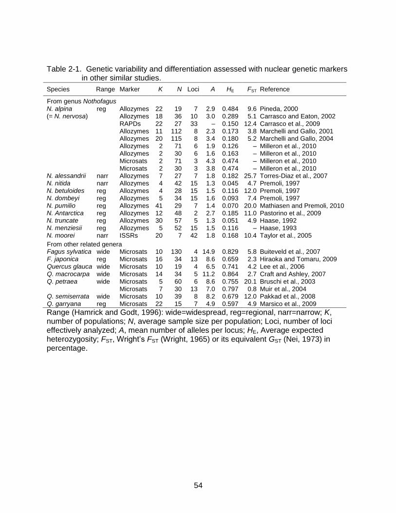
54
Table 2-1. Genetic variability and differentiation assessed with nuclear genetic markers in other similar studies.
Species Range Marker K N Loci A HE FST Reference
From genus Nothofagus N. alpina reg Allozymes 22 19 7 2.9 0.484 9.6 Pineda, 2000 (= N. nervosa) Allozymes 18 36 10 3.0 0.289 5.1 Carrasco and Eaton, 2002 RAPDs 22 27 33 – 0.150 12.4 Carrasco et al., 2009 Allozymes 11 112 8 2.3 0.173 3.8 Marchelli and Gallo, 2001 Allozymes 20 115 8 3.4 0.180 5.2 Marchelli and Gallo, 2004 Allozymes 2 71 6 1.9 0.126 – Milleron et al., 2010 Allozymes 2 30 6 1.6 0.163 – Milleron et al., 2010 Microsats 2 71 3 4.3 0.474 – Milleron et al., 2010 Microsats 2 30 3 3.8 0.474 – Milleron et al., 2010 N. alessandrii narr Allozymes 7 27 7 1.8 0.182 25.7 Torres-Diaz et al., 2007 N. nitida narr Allozymes 4 42 15 1.3 0.045 4.7 Premoli, 1997 N. betuloides reg Allozymes 4 28 15 1.5 0.116 12.0 Premoli, 1997 N. dombeyi reg Allozymes 5 34 15 1.6 0.093 7.4 Premoli, 1997 N. pumilio reg Allozymes 41 29 7 1.4 0.070 20.0 Mathiasen and Premoli, 2010 N. Antarctica reg Allozymes 12 48 2 2.7 0.185 11.0 Pastorino et al., 2009 N. truncate reg Allozymes 30 57 5 1.3 0.051 4.9 Haase, 1992 N. menziesii reg Allozymes 5 52 15 1.5 0.116 – Haase, 1993 N. moorei narr ISSRs 20 7 42 1.8 0.168 10.4 Taylor et al., 2005
From other related genera Fagus sylvatica wide Microsats 10 130 4 14.9 0.829 5.8 Buiteveld et al., 2007 F. japonica reg Microsats 16 34 13 8.6 0.659 2.3 Hiraoka and Tomaru, 2009 Quercus glauca wide Microsats 10 19 4 6.5 0.741 4.2 Lee et al., 2006 Q. macrocarpa wide Microsats 14 34 5 11.2 0.864 2.7 Craft and Ashley, 2007 Q. petraea wide Microsats 5 60 6 8.6 0.755 20.1 Bruschi et al., 2003 Microsats 7 30 13 7.0 0.797 0.8 Muir et al., 2004 Q. semiserrata wide Microsats 10 39 8 8.2 0.679 12.0 Pakkad et al., 2008 Q. garryana reg Microsats 22 15 7 4.9 0.597 4.9 Marsico et al., 2009
Range (Hamrick and Godt, 1996): wide=widespread, reg=regional, narr=narrow; K, number of populations; N, average sample size per population; Loci, number of loci effectively analyzed; A, mean number of alleles per locus; HE, Average expected heterozygosity; FST, Wright‟s FST (Wright, 1965) or its equivalent GST (Nei, 1973) in percentage.
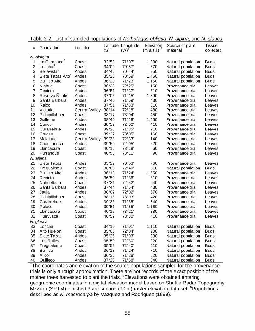
55
Table 2-2. List of sampled populations of Nothofagus obliqua, N. alpina, and N. glauca.
# Population Location Latitude (S)
†
Longitude (W)
†
Elevation (m a.s.l.)
†§
Source of plant material
Tissue collected
N. obliqua 1 La Campana
¢ Coast 32°58' 71°07' 1,380 Natural population Buds
2 Loncha¢ Coast 34°09' 70°57' 870 Natural population Buds
3 Bellavista¢ Andes 34°46' 70°44' 950 Natural population Buds
4 Siete Tazas Alto¢ Andes 35°28' 70°59' 1,460 Natural population Buds
5 Bullileo Alto Andes 36°20' 71°23' 1,150 Natural population Buds 6 Ninhue Coast 36°23' 72°25' 150 Provenance trial Leaves 7 Recinto Andes 36°51' 71°37' 710 Provenance trial Leaves 8 Reserva Ñuble Andes 37°06' 71°15' 1,890 Provenance trial Leaves 9 Santa Barbara Andes 37°40' 71°59' 430 Provenance trial Leaves
10 Ralco Andes 37°51' 71°33' 810 Provenance trial Leaves 11 Victoria Central Valley 38°14' 72°18' 480 Provenance trial Leaves 12 Pichipillahuen Coast 38°17' 73°04' 450 Provenance trial Leaves 13 Galletue Andes 38°40' 71°18' 1,450 Provenance trial Leaves 14 Cunco Andes 38°52' 72°00' 410 Provenance trial Leaves 15 Curarrehue Andes 39°25' 71°35' 910 Provenance trial Leaves 16 Cruces Coast 39°32' 73°05' 160 Provenance trial Leaves 17 Malalhue Central Valley 39°33' 72°33' 140 Provenance trial Leaves 18 Choshuenco Andes 39°50' 72°05' 220 Provenance trial Leaves 19 Llancacura Coast 40°16' 73°18' 60 Provenance trial Leaves 20 Purranque Coast 40°55' 73°11' 90 Provenance trial Leaves
N. alpina 21 Siete Tazas Andes 35°29' 70°53' 760 Provenance trial Leaves 22 Tregualemu Coast 36°03' 72°40' 510 Natural population Buds 23 Bullileo Alto Andes 36°18' 71°24' 1,650 Provenance trial Leaves 24 Recinto Andes 36°50' 71°36' 810 Provenance trial Leaves 25 Nahuelbuta Coast 37°31' 72°52' 940 Provenance trial Leaves 26 Santa Barbara Andes 37°44' 71°54' 430 Provenance trial Leaves 27 Jauja Andes 38°02' 72°02' 670 Provenance trial Leaves 28 Pichipillahuen Coast 38°18' 73°03' 420 Provenance trial Leaves 29 Curarrehue Andes 39°26' 71°35' 840 Provenance trial Leaves 30 Releco Andes 39°51' 71°55' 1,160 Provenance trial Leaves 31 Llancacura Coast 40°17' 73°21' 380 Provenance trial Leaves 32 Hueyusca Coast 40°59' 73°30' 410 Provenance trial Leaves
N. glauca 33 Loncha Coast 34°10' 71°01' 1,110 Natural population Buds 34 Alto Huelon Coast 35°06' 72°04' 200 Natural population Buds 35 Siete Tazas Andes 35°26' 71°03' 830 Natural population Buds 36 Los Ruiles Coast 35°50' 72°30' 220 Natural population Buds 37 Tregualemu Coast 35°59' 72°40' 510 Natural population Buds 38 Bullileo Andes 36°18' 71°24' 710 Natural population Buds 39 Alico Andes 36°35' 71°28' 620 Natural population Buds 40 Quilleco Andes 37°28' 71°58' 340 Natural population Buds †The coordinates and elevation of the source populations sampled for the provenance trials is only a rough approximation. There are not records of the exact position of the mother trees harvested to plant the trials. §Elevations were obtained entering geographic coordinates in a digital elevation model based on Shuttle Radar Topography Mission (SRTM) Finished 3 arc-second (90 m) raster elevation data set. ¢Populations described as N. macrocarpa by Vazquez and Rodriguez (1999).
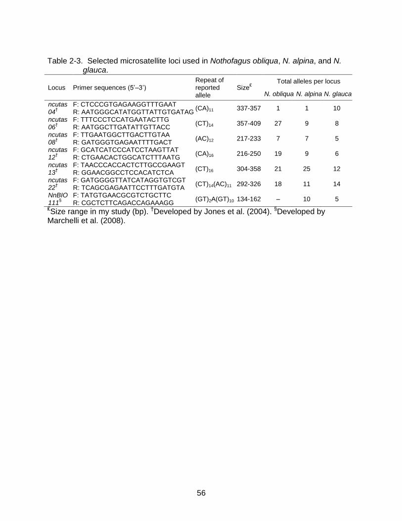
56
Table 2-3. Selected microsatellite loci used in Nothofagus obliqua, N. alpina, and N.
glauca.
Locus Primer sequences (5‟–3‟) Repeat of reported allele
Size₤
Total alleles per locus
N. obliqua N. alpina N. glauca
ncutas04
†
F: CTCCCGTGAGAAGGTTTGAAT R: AATGGGCATATGGTTATTGTGATAG
(CA)11 337-357 1 1 10
ncutas06
†
F: TTTCCCTCCATGAATACTTG R: AATGGCTTGATATTGTTACC
(CT)14 357-409 27 9 8
ncutas08
†
F: TTGAATGGCTTGACTTGTAA R: GATGGGTGAGAATTTTGACT
(AC)12 217-233 7 7 5
ncutas12
†
F: GCATCATCCCATCCTAAGTTAT R: CTGAACACTGGCATCTTTAATG
(CA)16 216-250 19 9 6
ncutas13
†
F: TAACCCACCACTCTTGCCGAAGT R: GGAACGGCCTCCACATCTCA
(CT)16 304-358 21 25 12
ncutas22
†
F: GATGGGGTTATCATAGGTGTCGT R: TCAGCGAGAATTCCTTTGATGTA
(CT)14(AC)11 292-326 18 11 14
NnBIO111
§
F: TATGTGAACGCGTCTGCTTC R: CGCTCTTCAGACCAGAAAGG
(GT)2A(GT)10 134-162 – 10 5
₤Size range in my study (bp). †Developed by Jones et al. (2004). §Developed by Marchelli et al. (2008).
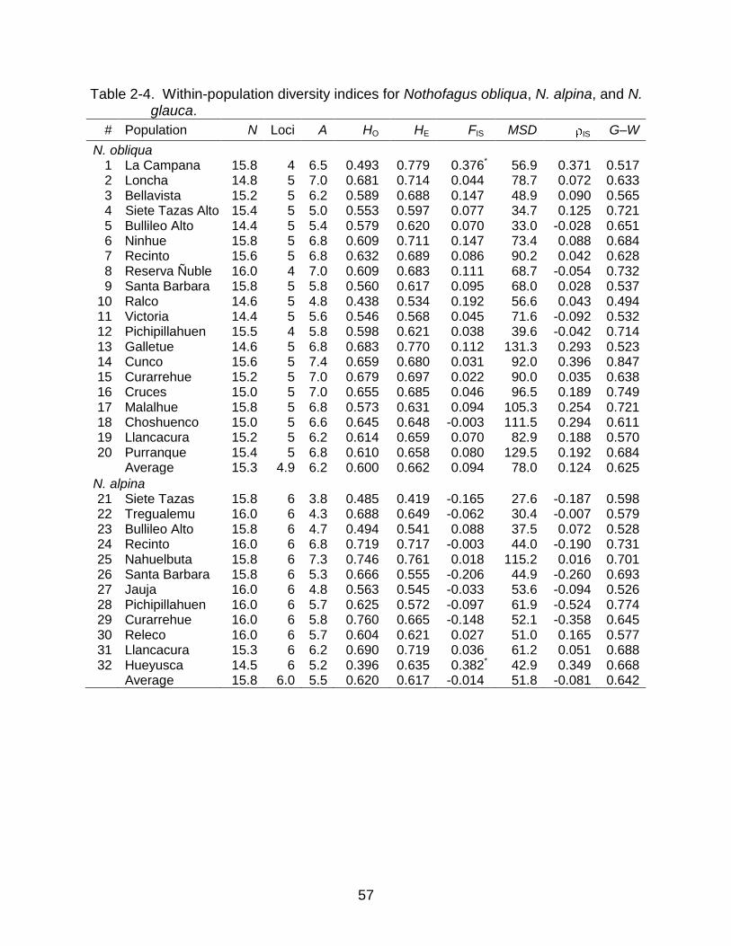
57
Table 2-4. Within-population diversity indices for Nothofagus obliqua, N. alpina, and N. glauca.
# Population N Loci A HO HE FIS MSD IS G–W
N. obliqua 1 La Campana 15.8 4 6.5 0.493 0.779 0.376* 56.9 0.371 0.517 2 Loncha 14.8 5 7.0 0.681 0.714 0.044 78.7 0.072 0.633 3 Bellavista 15.2 5 6.2 0.589 0.688 0.147 48.9 0.090 0.565 4 Siete Tazas Alto 15.4 5 5.0 0.553 0.597 0.077 34.7 0.125 0.721 5 Bullileo Alto 14.4 5 5.4 0.579 0.620 0.070 33.0 -0.028 0.651 6 Ninhue 15.8 5 6.8 0.609 0.711 0.147 73.4 0.088 0.684 7 Recinto 15.6 5 6.8 0.632 0.689 0.086 90.2 0.042 0.628 8 Reserva Ñuble 16.0 4 7.0 0.609 0.683 0.111 68.7 -0.054 0.732 9 Santa Barbara 15.8 5 5.8 0.560 0.617 0.095 68.0 0.028 0.537
10 Ralco 14.6 5 4.8 0.438 0.534 0.192 56.6 0.043 0.494 11 Victoria 14.4 5 5.6 0.546 0.568 0.045 71.6 -0.092 0.532 12 Pichipillahuen 15.5 4 5.8 0.598 0.621 0.038 39.6 -0.042 0.714 13 Galletue 14.6 5 6.8 0.683 0.770 0.112 131.3 0.293 0.523 14 Cunco 15.6 5 7.4 0.659 0.680 0.031 92.0 0.396 0.847 15 Curarrehue 15.2 5 7.0 0.679 0.697 0.022 90.0 0.035 0.638 16 Cruces 15.0 5 7.0 0.655 0.685 0.046 96.5 0.189 0.749 17 Malalhue 15.8 5 6.8 0.573 0.631 0.094 105.3 0.254 0.721 18 Choshuenco 15.0 5 6.6 0.645 0.648 -0.003 111.5 0.294 0.611 19 Llancacura 15.2 5 6.2 0.614 0.659 0.070 82.9 0.188 0.570 20 Purranque 15.4 5 6.8 0.610 0.658 0.080 129.5 0.192 0.684
Average 15.3 4.9 6.2 0.600 0.662 0.094 78.0 0.124 0.625
N. alpina 21 Siete Tazas 15.8 6 3.8 0.485 0.419 -0.165 27.6 -0.187 0.598 22 Tregualemu 16.0 6 4.3 0.688 0.649 -0.062 30.4 -0.007 0.579 23 Bullileo Alto 15.8 6 4.7 0.494 0.541 0.088 37.5 0.072 0.528 24 Recinto 16.0 6 6.8 0.719 0.717 -0.003 44.0 -0.190 0.731 25 Nahuelbuta 15.8 6 7.3 0.746 0.761 0.018 115.2 0.016 0.701 26 Santa Barbara 15.8 6 5.3 0.666 0.555 -0.206 44.9 -0.260 0.693 27 Jauja 16.0 6 4.8 0.563 0.545 -0.033 53.6 -0.094 0.526 28 Pichipillahuen 16.0 6 5.7 0.625 0.572 -0.097 61.9 -0.524 0.774 29 Curarrehue 16.0 6 5.8 0.760 0.665 -0.148 52.1 -0.358 0.645 30 Releco 16.0 6 5.7 0.604 0.621 0.027 51.0 0.165 0.577 31 Llancacura 15.3 6 6.2 0.690 0.719 0.036 61.2 0.051 0.688 32 Hueyusca 14.5 6 5.2 0.396 0.635 0.382* 42.9 0.349 0.668
Average 15.8 6.0 5.5 0.620 0.617 -0.014 51.8 -0.081 0.642
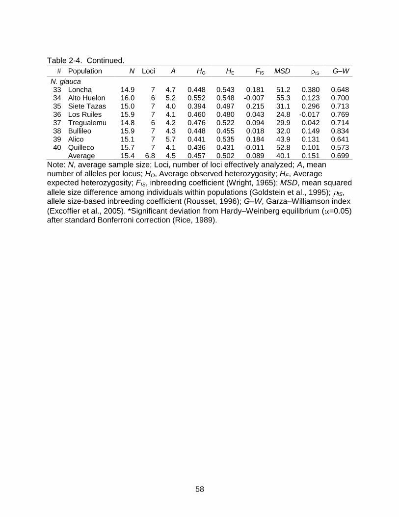
58
Table 2-4. Continued.
# Population N Loci A HO HE FIS MSD IS G–W
N. glauca 33 Loncha 14.9 7 4.7 0.448 0.543 0.181 51.2 0.380 0.648 34 Alto Huelon 16.0 6 5.2 0.552 0.548 -0.007 55.3 0.123 0.700 35 Siete Tazas 15.0 7 4.0 0.394 0.497 0.215 31.1 0.296 0.713 36 Los Ruiles 15.9 7 4.1 0.460 0.480 0.043 24.8 -0.017 0.769 37 Tregualemu 14.8 6 4.2 0.476 0.522 0.094 29.9 0.042 0.714 38 Bullileo 15.9 7 4.3 0.448 0.455 0.018 32.0 0.149 0.834 39 Alico 15.1 7 5.7 0.441 0.535 0.184 43.9 0.131 0.641 40 Quilleco 15.7 7 4.1 0.436 0.431 -0.011 52.8 0.101 0.573
Average 15.4 6.8 4.5 0.457 0.502 0.089 40.1 0.151 0.699
Note: N, average sample size; Loci, number of loci effectively analyzed; A, mean number of alleles per locus; HO, Average observed heterozygosity; HE, Average expected heterozygosity; FIS, inbreeding coefficient (Wright, 1965); MSD, mean squared
allele size difference among individuals within populations (Goldstein et al., 1995); IS, allele size-based inbreeding coefficient (Rousset, 1996); G–W, Garza–Williamson index
(Excoffier et al., 2005). *Significant deviation from Hardy–Weinberg equilibrium ( =0.05) after standard Bonferroni correction (Rice, 1989).
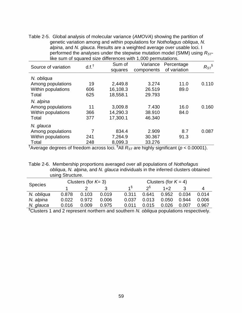
59
Table 2-5. Global analysis of molecular variance (AMOVA) showing the partition of
genetic variation among and within populations for Nothofagus obliqua, N. alpina, and N. glauca. Results are a weighted average over usable loci. I performed the analyses under the stepwise mutation model (SMM) using RST-like sum of squared size differences with 1,000 permutations.
Source of variation d.f.† Sum of
squares Variance
components Percentage of variation
RST§
N. obliqua Among populations 19 2,449.8 3.274 11.0 0.110 Within populations 606 16,108.3 26.519 89.0 Total 625 18,558.1 29.793
N. alpina
Among populations 11 3,009.8 7.430 16.0 0.160 Within populations 366 14,290.3 38.910 84.0 Total 377 17,300.1 46.340
N. glauca
Among populations 7 834.4 2.909 8.7 0.087 Within populations 241 7,264.9 30.367 91.3 Total 248 8,099.3 33.276
†Average degrees of freedom across loci. §All RST are highly significant (p < 0.00001). Table 2-6. Membership proportions averaged over all populations of Nothofagus
obliqua, N. alpina, and N. glauca individuals in the inferred clusters obtained using Structure.
Species Clusters (for K= 3)
Clusters (for K = 4)
1 2 3 1§ 2§ 1+2 3 4
N. obliqua 0.878 0.103 0.019 0.311 0.641 0.952 0.034 0.014 N. alpina 0.022 0.972 0.006 0.037 0.013 0.050 0.944 0.006 N. glauca 0.016 0.009 0.975 0.011 0.015 0.026 0.007 0.967 §Clusters 1 and 2 represent northern and southern N. obliqua populations respectively.
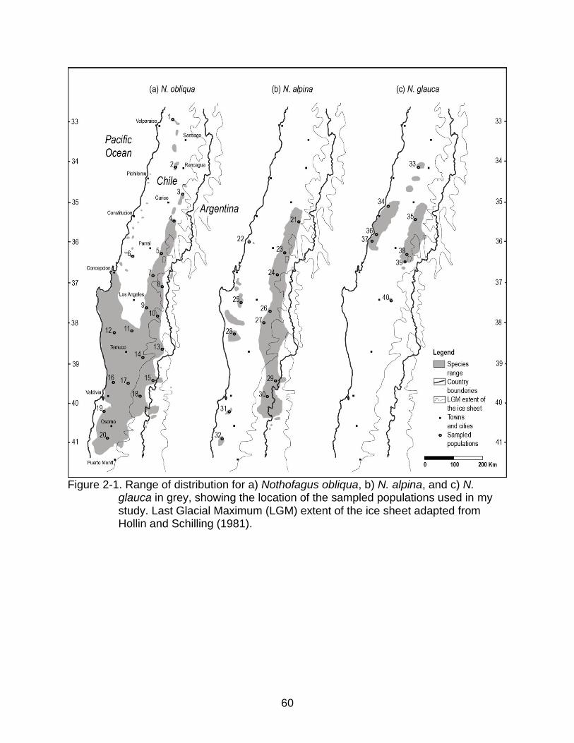
60
Figure 2-1. Range of distribution for a) Nothofagus obliqua, b) N. alpina, and c) N.
glauca in grey, showing the location of the sampled populations used in my study. Last Glacial Maximum (LGM) extent of the ice sheet adapted from Hollin and Schilling (1981).
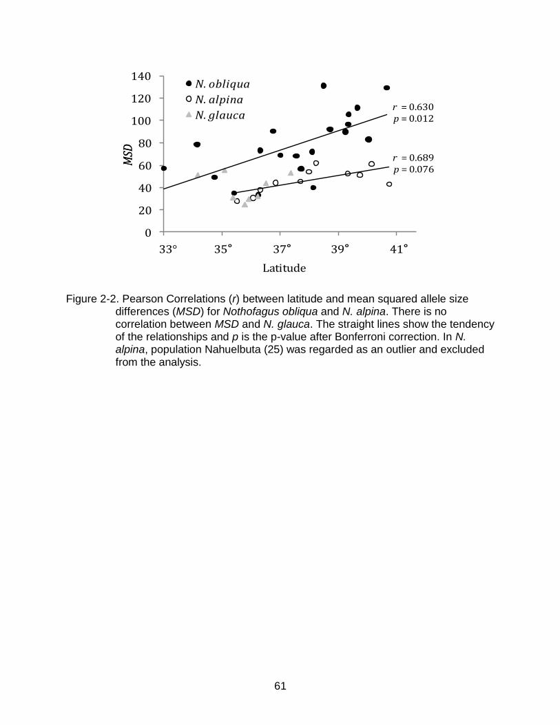
61
r = 0.630 p = 0.012
r = 0.689p = 0.076
0
20
40
60
80
100
120
140
0 230 460 690 920
N. obliqua
N. alpina
N. glauca
Latitude
MSD
MSD
33° 35° 37° 39° 41°
Figure 2-2. Pearson Correlations (r) between latitude and mean squared allele size differences (MSD) for Nothofagus obliqua and N. alpina. There is no correlation between MSD and N. glauca. The straight lines show the tendency of the relationships and p is the p-value after Bonferroni correction. In N. alpina, population Nahuelbuta (25) was regarded as an outlier and excluded from the analysis.
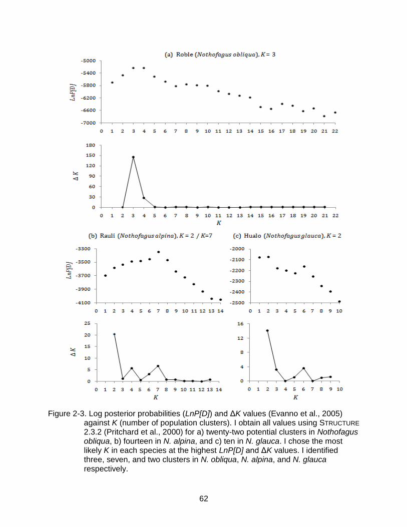
62
Figure 2-3. Log posterior probabilities (LnP[D]) and ΔK values (Evanno et al., 2005)
against K (number of population clusters). I obtain all values using STRUCTURE 2.3.2 (Pritchard et al., 2000) for a) twenty-two potential clusters in Nothofagus obliqua, b) fourteen in N. alpina, and c) ten in N. glauca. I chose the most likely K in each species at the highest LnP[D] and ΔK values. I identified three, seven, and two clusters in N. obliqua, N. alpina, and N. glauca respectively.
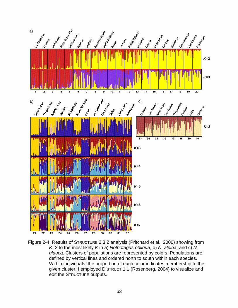
63
Figure 2-4. Results of STRUCTURE 2.3.2 analysis (Pritchard et al., 2000) showing from K=2 to the most likely K in a) Nothofagus obliqua, b) N. alpina, and c) N. glauca. Clusters of populations are represented by colors. Populations are defined by vertical lines and ordered north to south within each species. Within individuals, the proportion of each color indicates membership to the given cluster. I employed DISTRUCT 1.1 (Rosenberg, 2004) to visualize and edit the STRUCTURE outputs.
K=2
K=3
c)
a)
b)
K=3
K=4 K=5
K=6
K=7
K=2
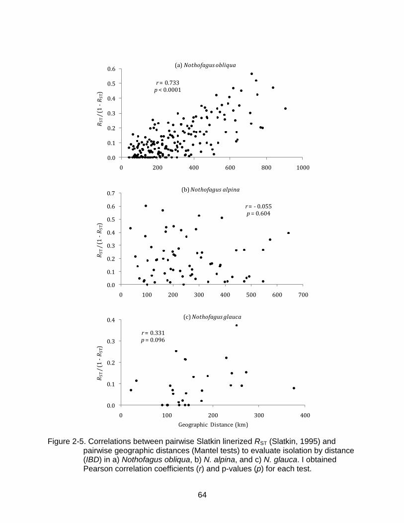
64
0.0
0.1
0.2
0.3
0.4
0.5
0.6
0 200 400 600 800 1000
RS
T /
(1
-R
ST)
r = 0.733p < 0.0001
0.0
0.1
0.2
0.3
0.4
0.5
0.6
0.7
0 100 200 300 400 500 600 700
RS
T /
(1
-R
ST)
r = - 0.055p = 0.604
(b) Nothofagus alpina
0.0
0.1
0.2
0.3
0.4
0 100 200 300 400
RS
T /
(1
-R
ST)
Geographic Distance (km)
r = 0.331p = 0.096
(c) Nothofagus glauca
(a) Nothofagus obliqua
Figure 2-5. Correlations between pairwise Slatkin linerized RST (Slatkin, 1995) and pairwise geographic distances (Mantel tests) to evaluate isolation by distance (IBD) in a) Nothofagus obliqua, b) N. alpina, and c) N. glauca. I obtained Pearson correlation coefficients (r) and p-values (p) for each test.
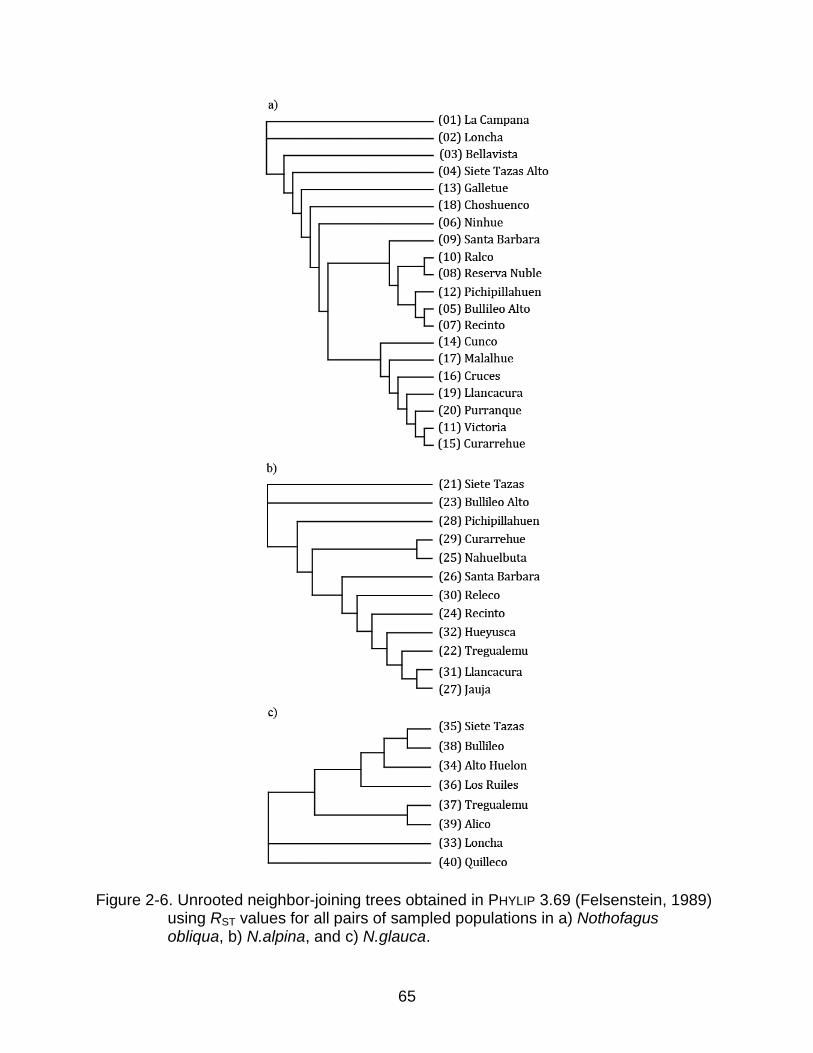
65
Figure 2-6. Unrooted neighbor-joining trees obtained in PHYLIP 3.69 (Felsenstein, 1989) using RST values for all pairs of sampled populations in a) Nothofagus obliqua, b) N.alpina, and c) N.glauca.
66
CHAPTER 3 MORPHOLOGICAL GENETIC VARIATION WITHIN AND AMONG PROVENANCES
OF NOTHOFAGUS OBLIQUA AND N. ALPINA GROWING IN CHILE. ADAPTIVE DIFFERENCES INFERRED FROM A PROVENANCE-PROGENY TRIAL
Introductory Remarks
Nothofagus obliqua (Mirb.) Oerst. and N. alpina (Poepp. et Endl.) Oerst. (= N.
nervosa) are two sympatric South American endemics belonging to subgenus
Lophozonia (Manos, 1997). These deciduous hardwood tree species are of remarkable
ecological and economic importance in Chile because of their role as habitat for many
plant and animal species, fast growth, and high-quality wood (Donoso, 1993).
Nothofagus obliqua and N. alpina forests cover as a whole about 1,000 km from north to
south between Valparaiso (33°00'S) and Puerto Montt (41°30'S) in Chile and adjacent
areas in Argentina (Figure 3-1), growing at different altitudes from the Central Valley to
the mountains (Ormazabal and Benoit, 1987).
These species grow in a range of climatic conditions depending on latitude and
elevation. In the northern part of their distribution in central Chile, habitat of the
Mediterranean Forests (33°00‟-36°30‟S), the climate is characterized by warm, dry, and
long summers. In these conditions, N. obliqua and N. alpina grow typically in the
mountains at elevations between 400 and 2,000 m a.s.l., and between 500 and 1,500 m
a.s.l. respectively, where there is enough precipitation for the species to survive
(Donoso, 1982). Conversely, in the southern part of their distribution, corresponding to
the Temperate Rainforests (south of 37°30'S), the climate becomes, in general, colder
and rainier with precipitations distributed year around and only a couple of months
relatively dry over the summer. Here, N. obliqua grows predominately from sea level to
400 m a.s.l., and N. alpina generally from 700 to 900 m a.s.l. (Veblen and Schlegel,
67
1982). Despite the two distinctive environmental conditions described above
corresponding to the main northern and southern forest types, the variation in
temperature and precipitations follow both latitudinal and altitudinal clines. According to
Di Castri and Hajek (1976), in this area the mean annual temperature at sea level
diminishes gradually north to south from 15°C to 10°C, and the mean annual
precipitation ranges from 300 to 1,500 mm depending on elevation in the north
increasing progressively southward where it ranges from 1,000 mm in the valleys to
3,000 mm or more in the west slopes of the mountains.
These climatic gradients are the most conspicuous reason why it is possible to
observe the phenotypic differences among provenances found in N. obliqua (Donoso,
1979; Ipinza et al., 2000) and N. alpina (Donoso, 1987; Medina, 2001), which show
clinal variation following those climatic gradients. Although the traits studied by these
authors (Donoso, 1979; 1987; Ipinza et al., 2000; Medina, 2001) are related to flowers
and fruits and therefore less likely to be affected by the environment (Clausen et al.,
1940), these patterns of variation could correspond to either plasticity or genetic
adaptation, because the experimental design of those studies does not allow separation
between the patterns of phenotypic diversity from those of genetic diversity.
Genetic diversity is one measure of biodiversity that allows a detailed description
of a populations‟ health. Genetic diversity is important in the forests because, in theory,
it helps the species to be resilient to disturbances such as fire, pests, and climate
change (White et al., 2007; Zobel and Talbert, 1984). Genetic diversity can be divided in
two major components: 1) Neutral variability, which is influenced by mutations, gene
flow, and genetic drift, but not affected by selection and therefore does not have
68
adaptive significance for the populations; and 2) Adaptive variability, which is
additionally and most importantly influenced by selection (McKay and Latta, 2002; White
et al., 2007).
Genetic variation within and between species is often analyzed using neutral
markers such as isozymes or molecular markers. The use of these techniques is
relatively inexpensive and fast (van Tienderen et al., 2002). Unfortunately, variability
obtained from the analysis of neutral markers has been shown to be uncorrelated with
adaptive variability obtained from the analysis of morphological traits (Reed and
Frankham, 2001; McKay and Latta, 2002). Adaptive genetic variation is a very important
component in populations, because whereas neutral variation determines the underlying
potential for longer-term evolutionary changes, adaptive variation determines the
evolutionary potential to respond to more immediate changes (McKay and Latta, 2002).
The main goal of my study is to evaluate the patterns of adaptive genetic variation
in N. obliqua and N. alpina, using quantitative traits related to adaptability to specific
environmental conditions, growth, and other morphological variables. I focus on
identifying the underlying factors that make up the adaptive genetic structure in these
two species.
I could not find any other study that examined the partitioning of genetic variances
among provenances versus the variance among families within provenances in
Nothofagus. However, this has been done in several other forest tree species. A review
examining some provenance-progeny tests in Castanea sativa (Tchatchoua and
Aravanopoulos, 2010a; 2010b), Swietenia macrophylla (Wightman et al., 2008), Pinus
palustris, Taxus brevifolia, and Populus trichocarpa (White et al., 2007), Gmelina
69
arborea (Hodge and Dvorak, 2004), Araucaria angustifolia (Sebbenn et al., 2003), Pinus
taeda (Sierra-Lucero et al., 2002), and Picea glauca (Li et al., 1993), shows that for
growth traits such as growth in height, stem diameter, and volume, the proportion of
among-provenance variance, as compared to the variance among families within
provenances, is considerable usually ranging between 40% and 80%. In other traits like
stem straightness, stem forking, and disease resistance, the proportion of among-
provenance variance is usually much lower than for growth traits, ranging from 0% to
50% indicating that for these variables in many cases almost all of the variation can be
found among families within a single provenance.
The amount of among-provenance adaptive genetic variation found in tree species
also depends on the ecological range where provenances grow. There is a tendency of
finding less among-provenance variation in species or groups of provenances growing
in regions that are ecologically homogeneous. For example, Xie (2008) reported the
among-provenance variation in growth traits for Alnus rubra finding that there was not a
statistically significant difference among provenances growing within each of two
ecologically homogeneous regions in the north and south of British Columbia, Canada,
indicating that virtually all the adaptive genetic variation within both regions was
allocated among families within provenances.
Despite the fact there is virtually no progeny-provenance studies analyzing the
partitioning of genetic variances in Nothofagus, there are several common garden
studies that analyze the significance of among-provenance variation and environmental
trends in morphological traits. In common garden studies there seems to be a tendency
to find more among-provenance variation in species with wider ecological ranges. In the
70
genus Nothofagus, those ranges are more or less associated to the different subgenera.
Thus, the species of subgenus Nothofagus have the wider ecological range, the species
of subgenus Fuscospora the narrower ecological range, and the species of subgenus
Lophozonia, which is the subgenus of N. obliqua and N. alpina, are somewhere in the
middle.
Among the species of subgenus Nothofagus, research in N. pumilio showed highly
significant among-provenance genetic differences between two elevations in shoot
length, leaf area, and leaf phenology (Premoli et al., 2007), as well as in stomatal
density (Premoli and Brewer, 2007), with the higher elevation having shorter shoots,
smaller leaves, late phenology, and less stomatal density. In subgenus Lophozonia, a
series of three papers in N. cunninghamii indicate that genetic differences in leaf area
among elevations were never significant, and that differences were significant in leaf
thickness and stomatal density with thicker leaves and less stomata per unit area at
higher elevations, but only when the range in elevation was wide enough (Hovenden,
2001; Hovenden and Vander Schoor, 2003; 2006). In N. menziesii, Sun and Sweet
(1996) found that provenances growing at higher elevations were genetically more frost
tolerant; Ledgard and Norton (1988) found that the growth period was significantly
shorter, ending sooner, and therefore plants were growing slower in provenances
exposed to lower temperatures; and Wilcox and Ledgard (1983) found significant
genetic variation among provenances in growth rate and leaf size. In N. obliqua, Puntieri
et al. (2006) found no significant among-provenance differences in growth rate, however
the ecological range of the analyzed provenances was very narrow. Finally, in species
of subgenus Fuscospora, there are fewer significant among-provenance differences
71
detected in adaptive traits. In N. alessandrii Santelices et al. (2009) found no significant
differences in growth rate. In N. fusca Wilcox and Ledgard (1983) found no significant
differences in growth rate or leaf size, and Ledgard and Norton (1988) found the same
for growth period, but some differences in growth rate. Finally, N. solandri, has among-
provenance differences in frost tolerance (Sun and Sweet, 1996), growth, and leaf size
(Ledgard and Norton, 1988; Wilcox and Ledgard, 1983), but not in growth period
(Ledgard and Norton, 1988).
My study is an attempt to genetically evaluate the patterns of variation in several
morphological traits for N. obliqua and N. alpina. The specific objectives of the study
are: a) to partition the species‟ morphological genetic variation among provenances and
among families within provenances, b) to find relationships between spatial patterns of
adaptive and climatic variability across the study area, c) to estimate the level of genetic
control or heritability on the variables measured in the trials, and d) to evaluate the
relative performance of provenances in growth traits.
I hypothesize that there will be higher levels of among-provenance variation in N.
obliqua than in N. alpina because of the wider ecological range in N. obliqua, and in
growth traits more than in form traits, the latter of which seem to have little adaptive
value. Also, I hypothesize that the patterns of among-provenance variation will follow a
latitudinal cline related to the climatic variation patterns in the study area and found by
other authors (Donoso, 1979; 1987; Ipinza et al., 2000; Medina, 2001). Finally, I expect
to find faster growth rates in provenances that originate in milder climates similar to the
conditions of the progeny-provenance trials.
72
In the summer of 2004 I measured one N. obliqua and one N. alpina progeny-
provenance trial, both established in the spring of 2000 by the FONDEF D96/1052
UACH-INFOR project in Fundo Arquilhue, Valdivia Province, Los Rios Region, Chile.
The trials contain one to 11 open-pollinated families from each of 31 and 14
provenances for N. obliqua and N. alpina respectively (Table 3-1). I measured survival,
total height, diameter, stem straightness, and stem forking on every four-year-old tree in
the trials. In a sub-sample, I measured leaf morphometrics related to leaf size, leaf
shape, and stomatal features.
Materials and Methods
Study Area, Seed Collection, and Trials General Description
I measured the offspring of open-pollinated mother trees belonging to
provenances systematically sampled by the project FONDEF D96/1052 (Universidad
Austral de Chile-Instituto Forestal) across most of the species range of distribution in
Chile (Figure 3-1) including the populations described as Nothofagus macrocarpa by
Vazquez and Rodriguez (1999) (Table 3-1), following Donoso (1979). In the summer of
1999, at each provenance, seeds from 10 mother trees were harvested. Trees were
selected maintaining a minimum distance of 100 m between them to maximize genetic
variation. After a pre-germination treatment, seeds were planted and grown in 80-mL
containers under greenhouse conditions for approximately seven months (Medina,
2001; Rodriguez and Medina, 2000). In the spring of 2000, the project simultaneously
planted one N. obliqua and one N. alpina progeny-provenance trial in Fundo Arquilhue,
property of the company “Agricola and Forestal Taquihue Ltda.”, located in the Valdivia
Province, Los Rios Region, Chile (40°14'S, 72°03'W, 304 m a.s.l.). The trials were
planted in a 4x2 m grid (i.e. density of 1,250 trees / ha), on a site with deep fertile
73
volcanic soils, a mean annual temperature of 9.8°C, and 3,500 mm in mean annual
precipitation. Due to restrictions in plant availability, the trials finally included between
one and 11 open-pollinated families from 31 N. obliqua and 14 N. alpina provenances
(Table 3-1).
Experimental Design, Measurements, and Data Editing
At the field location, both trials were planted in a randomized complete block
design (RCBD) using five complete blocks. Families from all provenances were placed
at random in each block using single-tree plots (STPs). The block sizes were 1 984 and
1,008 m2 for N. obliqua and N. alpina respectively, and there were two rows of plants
surrounding the trials to avoid uneven competition due to border effects.
In the summer of 2004, when trees were four years of age, I measured survival
(SURV), total height (HT in cm), stem diameter at the root collar (DIAM in mm), the
presence (1) or absence (0) of stem forking (FORK), and stem straightness using a
relative scale from very contorted (0) to very straight (4) (STR) on every tree in the
trials. I used HT and DIAM to calculate a volume index assuming a cone (R2H in L):
R2H = ((DIAM / 20)2 x HT) / 1000 (3-1)
Simultaneously, I obtained a sub-sample of five preformed and well-exposed
leaves from each tree on block one at each trial. I harvested, transported, and stored
the samples in a 4°C refrigerator in the Instituto de Silvicultura, Universidad Austral de
Chile. I first took surface impressions using clear nail polish from the abaxial leaf
surface between veins of one leaf from each tree. I mounted the impressions on
microscopy slides to measure stomatal length (SL in µm) in 10 stomata and stomatal
density (SD in stomata/mm2) in three microscopy fields using x400 and x160
magnification respectively (modified from Steubing et al. (2002)). Right after taking the
74
surface impressions, I scanned all the leaves creating digital images to later measure
leaf perimeter (LPER in cm) and leaf area (LAREA in cm2) using the PATCH ANALYST 3.1
extension for ARCGIS® 9.1 (Rempel and Carr, 2003), and number of lateral veins on the
leaf blade (LVEIN) counted by eye. Employing PATCH ANALYST I also calculated a shape
complexity index (SI) using LPER and LAREA:
SI = LPER / (2*π½*LAREA½) (3-2)
where SI=1 in a circle and is progressively larger than one when the shapes are more
irregular. Finally, and right after scanning, I dried all the leaves samples in an oven at
80°C overnight, and obtained dry weight (DW in g) for each 5-leaf sample (modified
from Steubing et al. (2002)). With this, I calculated leaf density (DENS in g/dm2) using:
DENS = (DW / LAREA)*100 (3-3)
I built two data sets with the variables subject to analysis. Data set 1 included
SURV, growth traits (HT, DIAM, and R2H), and form traits (FORK, and STR) from the
five blocks, and data set 2 included variables LAREA, LVEIN, DENS, SI, SL, and SD
from block one alone. Using SAS software 9.2 (SAS, 2008) I ran PROC UNIVARIATE to
detect suspected outliers by flagging observations that were at least three standard
deviations away from the variable mean. Also, I plotted the relationship between the
highly correlated HT and DIAM, to detect out-of-range data pairs. I re-measured the
suspicious observations or eliminated them in the cases where re-measurement was
not possible.
Analysis of Variance
Trials designed using RCBD with STPs are optimal in obtaining genetic structure
and parameter estimates (White et al., 2007). However, the variation in micro-site
conditions within a field test becomes a problem when the block size is too large and
75
the number of replicated blocks is small. In my STP-RCBD trials, the block sizes were
around 0.2 and 0.1 ha for N. obliqua and N. alpina respectively, and there were only five
replicates in each of them. In general, in standard forest sites the general rule is that the
block size should be less than 0.1 ha (Matheson, 1989), indicating that the block size for
N. obliqua was too large, and for N. alpina was at the limit. To solve this problem I
added the position of each tree in the trials using rows and columns as random effects
nested within blocks in the models as a way to account for the within-block spatial
variation (White et al., 2007).
Analysis of variables from all five blocks
For each species/variable combination, I compared nine different models using
restricted maximum likelihood analysis (REML) in PROC MIXED in SAS 9.2 (SAS, 2008). I
used the Bayesian Information Criterion (BIC) (Schwarz, 1978) to find the optimal model
maximizing likelihood and accounting for overfitting. I started with the simplest model
with no effects, and then progressively I added the fixed effect of the provenance, and
the random effects of block, provenance by block interaction, family nested within
provenance, row nested within blocks, and column nested within blocks. I additionally
ran all the models that included the block effect allowing heterogeneous variance
among blocks. Here I show the full model including all the effects:
yijklm = + i + j + ( )ij + (i)k + (j)l + (j)m + ijklm (3-4)
where
yijklm = phenotype of the kth family from the ith provenance in the lth row and mth column
within the jth block,
= overall mean,

76
i = fixed effect of the ith provenance,
j = random effect of the jth block,
( )ij = random interaction of the ith provenance and the jth block,
(i)k = random effect of the kth family within the ith provenance,
(j)l = random effect of the lth row within the jth block,
(j)m = random effect of the mth column within the jth block, and
ijklm = random residual error.
After finding the best model for each variable, I ran the analyses treating all effects
but provenance as random to estimate the provenances least square means (LSM) and
to obtain significance of the among-provenances differences. I also ran the models
treating provenance as a random effect to obtain the partition of variation among
provenance and among families within provenances. In PROC MIXED I used the
Kenward-Roger method to test the significance of fixed effects, and asymptotic t tests to
evaluate random effects.
Analysis of variables from block one
I used the same approach as above to analyze these variables, but eliminating the
family and block effects from the models. Thus, for each species/variable combination, I
compared five different models. I started with the simplest model with no effects, and
then progressively I added the fixed effect of the provenance, and the random effects of
row and column. Here, the full model is:
yijkl = + i + j + k + ijkl (3-5)
where
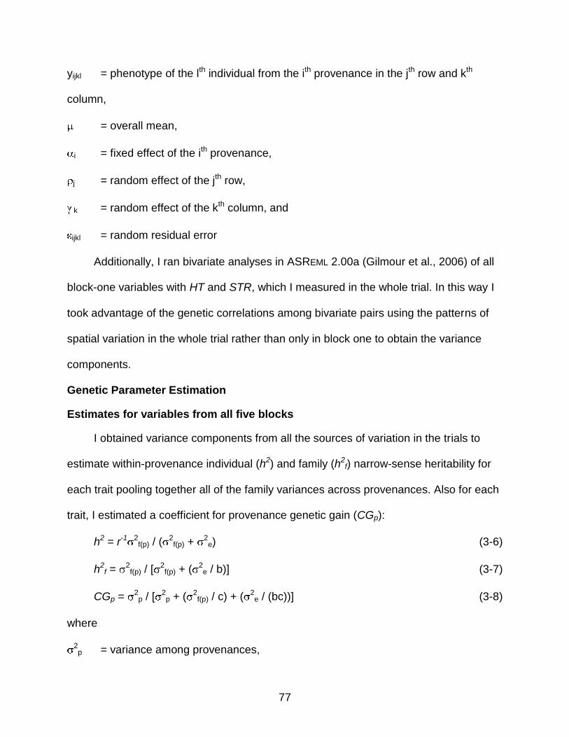
77
yijkl = phenotype of the lth individual from the ith provenance in the jth row and kth
column,
= overall mean,
i = fixed effect of the ith provenance,
j = random effect of the jth row,
k = random effect of the kth column, and
ijkl = random residual error
Additionally, I ran bivariate analyses in ASREML 2.00a (Gilmour et al., 2006) of all
block-one variables with HT and STR, which I measured in the whole trial. In this way I
took advantage of the genetic correlations among bivariate pairs using the patterns of
spatial variation in the whole trial rather than only in block one to obtain the variance
components.
Genetic Parameter Estimation
Estimates for variables from all five blocks
I obtained variance components from all the sources of variation in the trials to
estimate within-provenance individual (h2) and family (h2f) narrow-sense heritability for
each trait pooling together all of the family variances across provenances. Also for each
trait, I estimated a coefficient for provenance genetic gain (CGp):
h2 = r-1 2f(p) / (
2f(p) + 2
e) (3-6)
h2f = 2
f(p) / [2f(p) + ( 2
e / b)] (3-7)
CGp = 2p / [
2p + ( 2
f(p) / c) + ( 2e / (bc))] (3-8)
where
2p = variance among provenances,

78
2f(p) = variance among families within provenance,
2e = error variance,
r = coefficient of relationship,
b = harmonic mean of the number of individuals per family, and
c = harmonic mean of the number of families per provenance.
I adjusted the coefficient of relationship for half-sib families (r = 0.25) following Squillace
(1974). The selfing rate estimates for Nothofagus varied from 2% to 6% in a controlled
pollination study (Riveros et al., 1995) and in an allozyme study (Gallo et al., 1997).
Therefore, considering a selfing rate of 5%, and assuming about 10 local unrelated
pollen donors, and less than 10 non-local pollen donors, the adjusted r was 0.29,
significantly smaller than the conservative r = 0.35 used for Nothofagus by Ipinza et al.
(2000). In my analysis I used r = 0.29 to obtain additive variances and calculate h2, and
compared these values with the ones obtained using r = 0.35.
To obtain the partition of variation within and among provenances, I estimated the
proportion of the total morphological genetic variation that is due to differences among
provenances using:
= 2p / (
2p + 2
f(p)) (3-9)
where
= proportion of among-provenance variation,
2p = variance among provenances, and
2f(p) = variance among families within provenance.
79
Estimates for variables from block one
For this analysis, I only obtained variance components to estimate the coefficient
for provenance genetic gain (CGp). Here, I could not obtain the partition of variation
among provenance and among families within provenances. I compared results
obtained from both the univariate analysis ran on SAS and the bivariate analysis ran on
ASREML.
Among-Provenance Differentiation
When I treated the effects of provenance as fixed effects, I could estimate least
square means (LSM) for each variable / provenance combination and obtain the
significance of the differences among provenances. Using LSM, I ran multiple
comparison tests among groups of provenances applying the standard Bonferroni
correction for multiple comparisons (Rice, 1989) at each variable. I grouped the
provenances in two ways. First, according to their geographic origin I found three
groups; provenances from the Mediterranean Forests (33°00‟-36°30‟S), from the
Transitional Forests (36°30‟-38°00‟S), and from the Temperate Rainforests (38°00'-
41°30‟S). And second, according to a non-hierarchical cluster analysis performed using
the provenances mean annual temperature (MAT) and mean annual precipitation (MAP)
(Table 3-1).
I also obtained correlations among family and provenance LSM for single
morphological variables and MAT, MAP, and the absolute differences in MAT between
the trial site and the provenance origin (DMAT). Due to the low sample size to test the
significance of the correlations using provenance LSM (n=31 and n=14 for N. obliqua
and N. alpina respectively) I only tested the dependent variables HT, DENS, SL, and
SD, which were non-multicolinear and most adaptively meaningful.
80
Canonical Correlation, Discriminant, and Cluster Analysis
All multivariate analysis procedures used in this Section: PROC CANCOR, PROC
STEPDISC, PROC DISCRIM, PROC VARCLUS, PROC FASTCLUS, and PROC CLUSTER are part of
SAS 9.2 (SAS, 2008) and were chosen following McGarigal et al., (2000).
Analysis at the provenance level
I first employed canonical correlation in PROC CANCOR to see how the combination
of the environmental variables MAT and MAP were correlated to the morphological
variables using squared canonical correlations and significance values. In addition, the
standardized canonical coefficients identified which morphological and environmental
variables contributed the most to each canonical variable.
Also, as a way to define groups of provenances integrating the environmental
variables MAT and MAP I performed cluster analyses using standardized values (z-
scores) of both of these variables. I used PROC FASTCLUS to run non-hierarchical cluster
analyses to obtain a stable solution for the number of clusters or groups. I compared the
pseudo-F statistic (Pseudo-F) and the cubic clustering criterion (CCC) simultaneously
among solutions to choose the optimal number of groups. After finding the optimal
number of provenance groups, I ran stepwise discriminant analysis (DA) in PROC
STEPDISC to correlate group membership of provenances with the provenance LSM of
the non-multicolinear morphological variables allowing variables to enter and to stay in
the model if p-value ≤ 0.15. To separate multicolinear variables before the DA, I
conducted a hierarchical cluster analysis on the morphological variables using
correlation matrices in PROC VARCLUS. I input the significant variables identified with
PROC STEPDISC in PROC DISCRIM to obtain the posterior probability of membership in
groups and to run a cross-validation assessing the homogeneity of group dispersions.
81
Finally, to obtain dendrograms indicating closeness in adaptive traits among
provenances I first performed non-hierarchical cluster analyses in PROC FASTCLUS
combining all non-multicolinear morphological traits to obtain a stable solution for the
membership in main clusters. I compared the pseudo-F statistic (Pseudo-F) and the
cubic clustering criterion (CCC) simultaneously among solutions to choose the optimal
number of groups using standardized values of the provenance LSM (z-scores). Then, I
performed hierarchical cluster analyses in PROC CLUSTER testing several clustering
methods (i.e. average linkage, centroid, complete linkage, single linkage, and Ward‟s
minimum-variance). I chose the dendrogram from the method that had the best match in
main clusters with the grouping obtained from the more stable non-hierarchical cluster
analyses.
Analysis at the family level
Similar to the analysis at the provenance level, I ran stepwise DA in PROC
STEPDISC to correlate provenance membership of families with the family LSM of the
non-multicolinear morphological variables and then I used PROC DISCRIM to obtain the
posterior probability of membership in provenances and to run a cross-validation
assessing the homogeneity of provenance dispersions.
Results
Best Models for the Analysis of Variance
Using the Bayesian Information Criterion (BIC) (Schwarz, 1978), I chose the best
of nine models for each species/variable combination. For the variables measured in all
five blocks, I choose three models. For STR in Nothofagus obliqua and HT, DIAM, and
R2H in N. obliqua and N. alpina the optimal model was:
yijklm = + i + j + (i)k + (j)l + (j)m + ijklm (allowing HVAB) (3-10)

82
For FORK in N. obliqua and STR in N. alpina:
yijk = + i + j + (i)k + ijk (allowing HVAB) (3-11)
Finally, for FORK in N. alpina:
yij = + i + j + ij (3-12)
where
yijklm = phenotype of the kth family from the ith provenance in the lth row and mth column
within the jth block,
= overall mean,
i = fixed effect of the ith provenance,
j = random effect of the jth block,
(i)k = random effect of the kth family within the ith provenance,
(j)l = random effect of the lth row within the jth block,
(j)m = random effect of the mth column within the jth block,
ijklm = random residual error, and
HVAB = heterogeneous variance among blocks.
Likewise, for the variables measured only in block one, I choose three models. For
LVEIN, SI, SL, and SD in N. obliqua and LVEIN, DENS, and SD in N. alpina the optimal
model was:
yikl = + i + k + ikl (3-13)
For LAREA in N. obliqua and SL in N. alpina:
yijl = + i + j + ijl (3-14)
Finally, for DENS in N. obliqua and LAREA and SI in N. alpina:
83
yil = + i + il (3-15)
where
yijkl = phenotype of the lth individual from the ith provenance in the jth row and kth
column,
= overall mean,
i = fixed effect of the ith provenance,
j = random effect of the jth row,
k = random effect of the kth column, and
ijkl = random residual error
Genetic Parameter Estimates
With the variance components obtained from the analysis of the chosen models I
obtained the genetic parameter values shown in Tables 3-2 and 3-3. Within-provenance
individual (h2) and family (h2f) narrow-sense heritabilities were substantial for all
variables in N. obliqua and for HT and STR in N. alpina. In N. alpina the heritabilities for
DIAM and R2H were low and FORK had no heritability. Also, values were consistently
higher in N. obliqua than in N. alpina for all variables (Table 3-2). The values of the
coefficient for provenance genetic gain (CGp) were in general much higher than the
values for heritabilities and higher in N. obliqua than in N. alpina, except for FORK,
STR, LAREA, and SI (Tables 3-2 and 3-3). The values were all greater than 0.5
except for FORK in N. obliqua ( =0) indicating that the proportion of the among-
provenance variation was usually greater than the proportion of the among-family
variation (Table 3-2).
84
The narrow-sense genetic correlations among traits (rA) are shown in Table 3-4.
There was a wide range of rA values among variables, but the correlations of trait pairs
HT/SL, STR/SI, STR/SL in N. obliqua and HT/SL, STR/SL, STR/SD in N. alpina were
greater than 0.75 and are regarded as strong.
Among-Provenance Differentiation
Using the provenance LSM for all traits (Table 3-5) I tested the statistical
significance of the differences among provenances. Differentiation among provenances
in N. obliqua was not significant ( >0.05) for FORK and SL, significant ( <0.05) for SI,
and SD, and highly significant ( <0.01) for all other variables including the growth traits
(HT, DIAM, R2H). Conversely, in N. alpina the differences among provenances were
highly significant only for HT and STR, significant for DIAM, R2H, LAREA, and SI, and
not significant for all other variables (Table 3-6).
These significant differences imply that at least one provenance was different than
the average value of all provenances. To avoid performing too many multiple
comparisons among all provenances in each species, which would seriously hinder the
power of the tests, I used contrast analysis to compare groups of provenances defined
by latitudinal differences in type of forests (Mediterranean Forests, Transitional Forests,
and Temperate Rainforests) and defined by a non-hierarchical cluster analysis based
on environmental variables (MAT and MAP) that found three groups of provenances for
N. obliqua and two for N. alpina (Figure 3-2). Results in Figure 3-3 show that for N.
obliqua HT, DIAM, and R2H were significantly lower (p<0.0006) in the Mediterranean
Forests than in the other two zones. Also SL had the same pattern, but the values were
higher in the Mediterranean Forests (p=0.045). The variables STR and LAREA and SI
85
did not follow the same tendency, however the values were still lower in the
Mediterranean Forests than in the Temperate Rainforests (p<0.0006, p=0.018, and
p=0.003 respectively).
I also found for N. obliqua that HT, DIAM, and R2H were significantly higher
(p<0.0006) in Warm and Rainy provenances than in the other two groups (Figure 3-4).
In the case of SL, the Warm and Rainy provenances were only significantly lower in
value than the Warm and Dry group (p=0.026), and in SD the values were only
significantly lower than the Cold and Rainy group (p=0.006).
For N. alpina I did not find any geographic or environmental pattern of variation in
any of the putatively adaptive traits like the growth traits, LAREA, DENS, SL, or SD. The
only significant differences were found between the Mediterranean Forests and the
Temperate Rainforests in SI (Figure 3-5). The values of SI were lower in the Temperate
Rainforests (p=0.013).
Patterns of Variation Related to Single Environmental Variables
I obtained Pearson correlations (r) and their significance using Bonferroni
corrections of provenance and family least square means (LSM) for HT, DENS, SL, and
SD with MAT, MAP, and DMAT to detect possible trends of adaptation to the
environmental variables. In N. obliqua I found a trend of increased HT with an increment
in MAP using the provenance LSM (Figure 3-6a, r=0.45, p=0.132, n=31). Although r
was not significant at this level, the correlation using family LSM was consistent with
that result becoming highly significant due to the increase in the number of observations
(Fig, 6b, r=0.26, p<0.0001, n=247). Something similar occurred with the correlation
between SD and MAT (Figure 3-6c and d) but in this case the increase in the number of
observation (from n=31 to n=247) did not improve the significance of the correlation
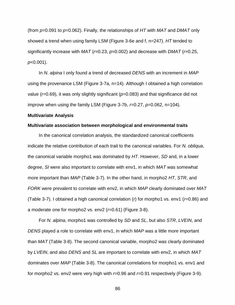
86
(from p=0.091 to p=0.062). Finally, the relationships of HT with MAT and DMAT only
showed a trend when using family LSM (Figure 3-6e and f, n=247). HT tended to
significantly increase with MAT (r=0.23, p=0.002) and decrease with DMAT (r=0.25,
p<0.001).
In N. alpina I only found a trend of decreased DENS with an increment in MAP
using the provenance LSM (Figure 3-7a, n=14). Although I obtained a high correlation
value (r=0.69), it was only slightly significant (p=0.083) and that significance did not
improve when using the family LSM (Figure 3-7b, r=0.27, p=0.062, n=104).
Multivariate Analysis
Multivariate association between morphological and environmental traits
In the canonical correlation analysis, the standardized canonical coefficients
indicate the relative contribution of each trait to the canonical variables. For N. obliqua,
the canonical variable morpho1 was dominated by HT. However, SD and, in a lower
degree, SI were also important to correlate with env1, in which MAT was somewhat
more important than MAP (Table 3-7). In the other hand, in morpho2 HT, STR, and
FORK were prevalent to correlate with env2, in which MAP clearly dominated over MAT
(Table 3-7). I obtained a high canonical correlation (r) for morpho1 vs. env1 (r=0.86) and
a moderate one for morpho2 vs. env2 (r=0.61) (Figure 3-8).
For N. alpina, morpho1 was controlled by SD and SL, but also STR, LVEIN, and
DENS played a role to correlate with env1, in which MAP was a little more important
than MAT (Table 3-8). The second canonical variable, morpho2 was clearly dominated
by LVEIN, and also DENS and SL are important to correlate with env2, in which MAT
dominates over MAP (Table 3-8). The canonical correlations for morpho1 vs. env1 and
for morpho2 vs. env2 were very high with r=0.96 and r=0.91 respectively (Figure 3-9).
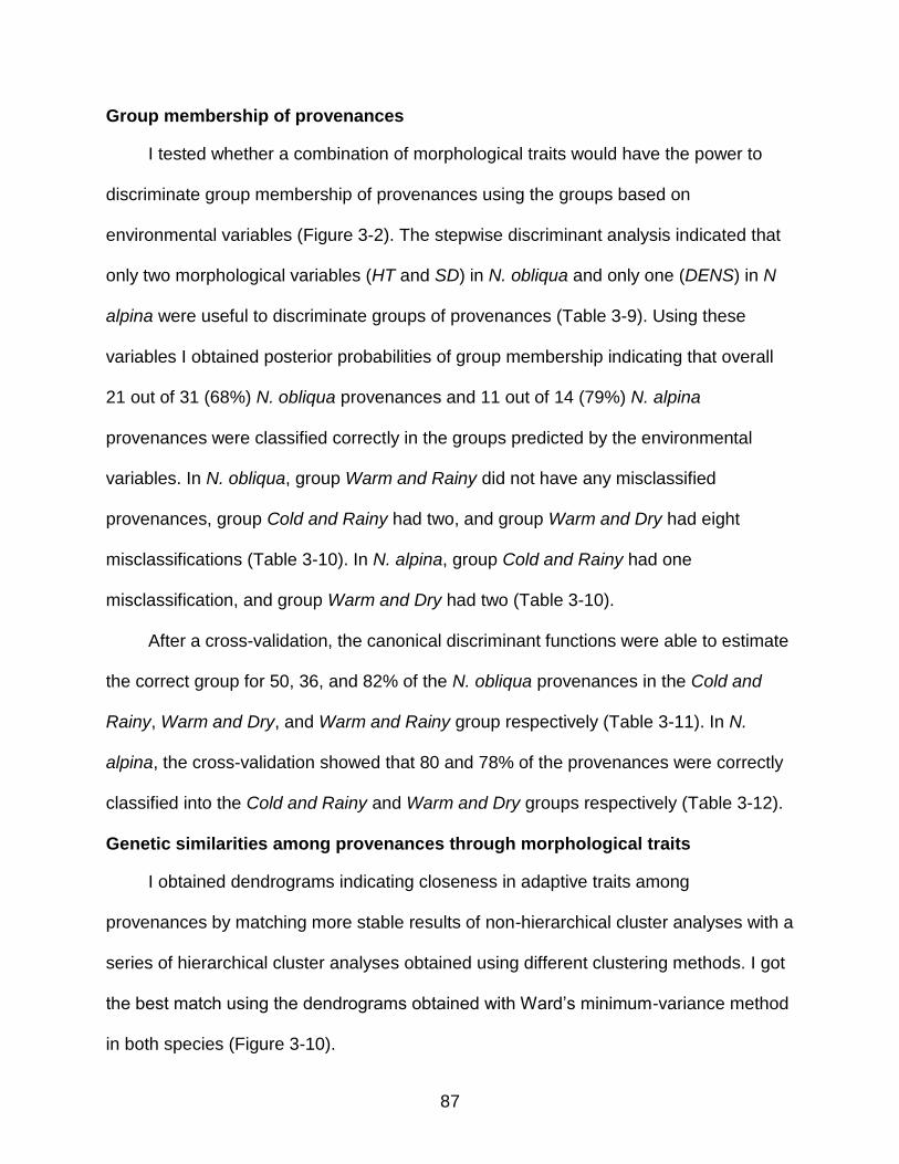
87
Group membership of provenances
I tested whether a combination of morphological traits would have the power to
discriminate group membership of provenances using the groups based on
environmental variables (Figure 3-2). The stepwise discriminant analysis indicated that
only two morphological variables (HT and SD) in N. obliqua and only one (DENS) in N
alpina were useful to discriminate groups of provenances (Table 3-9). Using these
variables I obtained posterior probabilities of group membership indicating that overall
21 out of 31 (68%) N. obliqua provenances and 11 out of 14 (79%) N. alpina
provenances were classified correctly in the groups predicted by the environmental
variables. In N. obliqua, group Warm and Rainy did not have any misclassified
provenances, group Cold and Rainy had two, and group Warm and Dry had eight
misclassifications (Table 3-10). In N. alpina, group Cold and Rainy had one
misclassification, and group Warm and Dry had two (Table 3-10).
After a cross-validation, the canonical discriminant functions were able to estimate
the correct group for 50, 36, and 82% of the N. obliqua provenances in the Cold and
Rainy, Warm and Dry, and Warm and Rainy group respectively (Table 3-11). In N.
alpina, the cross-validation showed that 80 and 78% of the provenances were correctly
classified into the Cold and Rainy and Warm and Dry groups respectively (Table 3-12).
Genetic similarities among provenances through morphological traits
I obtained dendrograms indicating closeness in adaptive traits among
provenances by matching more stable results of non-hierarchical cluster analyses with a
series of hierarchical cluster analyses obtained using different clustering methods. I got
the best match using the dendrograms obtained with Ward‟s minimum-variance method
in both species (Figure 3-10).
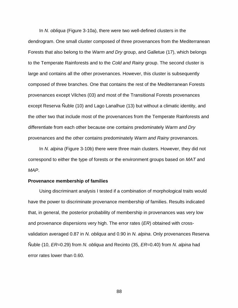
88
In N. obliqua (Figure 3-10a), there were two well-defined clusters in the
dendrogram. One small cluster composed of three provenances from the Mediterranean
Forests that also belong to the Warm and Dry group, and Galletue (17), which belongs
to the Temperate Rainforests and to the Cold and Rainy group. The second cluster is
large and contains all the other provenances. However, this cluster is subsequently
composed of three branches. One that contains the rest of the Mediterranean Forests
provenances except Vilches (03) and most of the Transitional Forests provenances
except Reserva Ñuble (10) and Lago Lanalhue (13) but without a climatic identity, and
the other two that include most of the provenances from the Temperate Rainforests and
differentiate from each other because one contains predominately Warm and Dry
provenances and the other contains predominately Warm and Rainy provenances.
In N. alpina (Figure 3-10b) there were three main clusters. However, they did not
correspond to either the type of forests or the environment groups based on MAT and
MAP.
Provenance membership of families
Using discriminant analysis I tested if a combination of morphological traits would
have the power to discriminate provenance membership of families. Results indicated
that, in general, the posterior probability of membership in provenances was very low
and provenance dispersions very high. The error rates (ER) obtained with cross-
validation averaged 0.87 in N. obliqua and 0.90 in N. alpina. Only provenances Reserva
Ñuble (10, ER=0.29) from N. obliqua and Recinto (35, ER=0.40) from N. alpina had
error rates lower than 0.60.
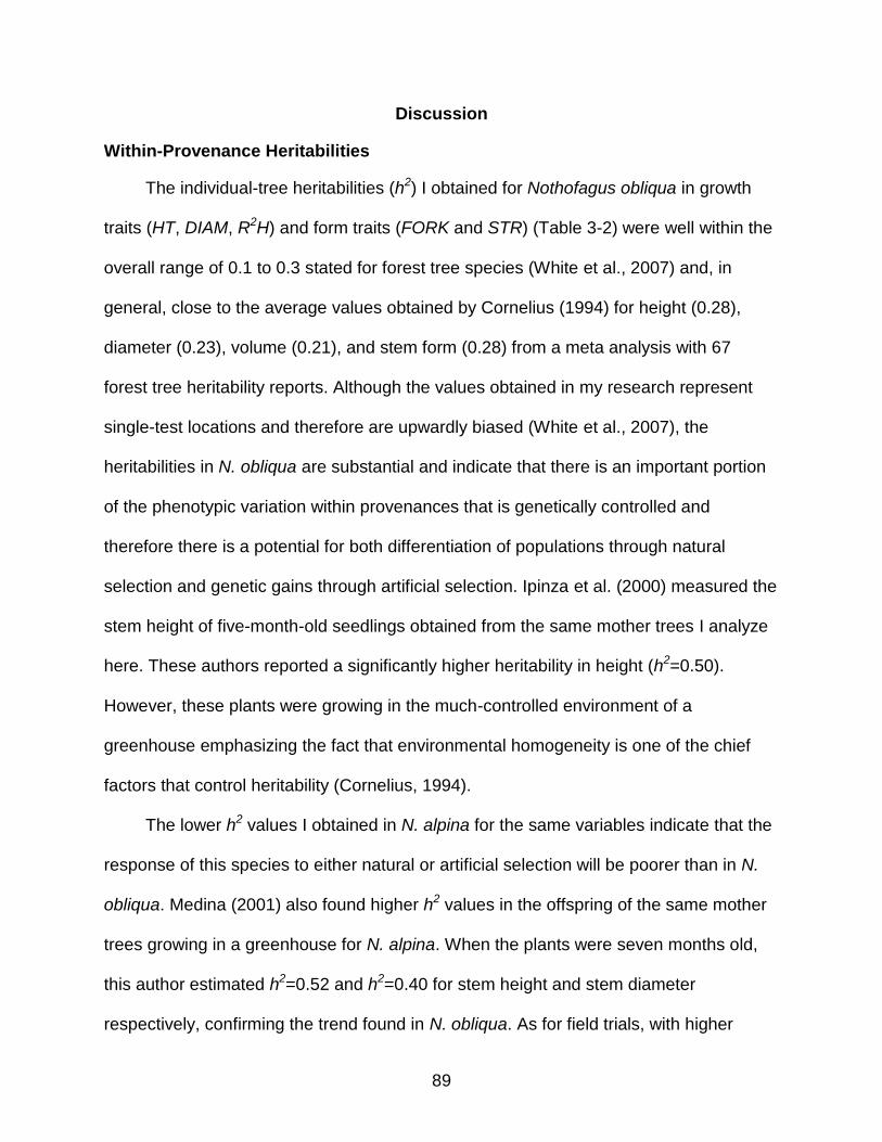
89
Discussion
Within-Provenance Heritabilities
The individual-tree heritabilities (h2) I obtained for Nothofagus obliqua in growth
traits (HT, DIAM, R2H) and form traits (FORK and STR) (Table 3-2) were well within the
overall range of 0.1 to 0.3 stated for forest tree species (White et al., 2007) and, in
general, close to the average values obtained by Cornelius (1994) for height (0.28),
diameter (0.23), volume (0.21), and stem form (0.28) from a meta analysis with 67
forest tree heritability reports. Although the values obtained in my research represent
single-test locations and therefore are upwardly biased (White et al., 2007), the
heritabilities in N. obliqua are substantial and indicate that there is an important portion
of the phenotypic variation within provenances that is genetically controlled and
therefore there is a potential for both differentiation of populations through natural
selection and genetic gains through artificial selection. Ipinza et al. (2000) measured the
stem height of five-month-old seedlings obtained from the same mother trees I analyze
here. These authors reported a significantly higher heritability in height (h2=0.50).
However, these plants were growing in the much-controlled environment of a
greenhouse emphasizing the fact that environmental homogeneity is one of the chief
factors that control heritability (Cornelius, 1994).
The lower h2 values I obtained in N. alpina for the same variables indicate that the
response of this species to either natural or artificial selection will be poorer than in N.
obliqua. Medina (2001) also found higher h2 values in the offspring of the same mother
trees growing in a greenhouse for N. alpina. When the plants were seven months old,
this author estimated h2=0.52 and h2=0.40 for stem height and stem diameter
respectively, confirming the trend found in N. obliqua. As for field trials, with higher
90
environmental variation, there are estimates of h2=0.07 for stem diameter and stem
height in a 1-year-old progeny test of N. alpina (Gutiérrez and Ipinza, 2000), which are
comparable with the values obtained in the current study.
Comparing h2 estimates among traits, there is a general trend for height and form
to have higher values than for diameter and volume (Cornelius, 1994; White et al.,
2007), probably because growth in diameter and, consequently, in volume have an
extra environmental source of variation when the trial density is uneven. I observed this
trend in N. alpina but not in N. obliqua where the h2 estimates were considerably higher
in DIAM and R2H than in HT. I do not have an explanation for these unexpected results
provided that the N. obliqua and N. alpina trails were planted at the same density and
overall survival was only slightly better in N. obliqua (97%) than in N. alpina (94%).
The h2 estimates obtained using the coefficients of relationship r=0.29 defined in
my study are slightly higher than the estimates obtained using the more conservative
r=0.35 defined by Ipinza et al. (2000), but do not change the trends of my results.
However, it would be wise to use the conservative estimates when projecting future
genetic gains of individual selections in a genetic improvement program. For that
matter, the family heritability (h2f) is also important for its use in selection indices
because it is typically larger than h2 and therefore can improve selection efficiency. The
h2f estimates in N. obliqua and N. alpina are larger than the h2 estimates however, the
differences are not that significant to take advantage of them in a selection index. The
reason for this is that the trials have only five replicates to obtain h2f.
Genetic Correlations among Traits
Obtaining genetic correlations among traits (rA) was not a goal in my study but as I
ran the bivariate analysis in ASREML (Gilmour et al., 2006) to obtain better estimates of
91
the variance components in the block-one variables, I obtained values for rA (Table 3-4).
Genetic correlations are a measure of pleiotropy. Thus, traits with a strong rA are
influenced by a similar set of genes and therefore changes in the allelic frequency of
those genes will influence both traits (White et al. 2007).
For example, the strong rA estimates I obtained between HT and SL would imply
that any time there is a selective pressure to increase height growth in N. obliqua or N.
alpina there would be a decrease or an increase in stomatal length respectively. Having
strong trait-trait genetic correlations like these could have interesting ecological and
economical implications. In my example, assuming that measures of SL do not vary with
age, I could potentially use SL for early selection of HT in one-year old N. obliqua or N.
alpina seedlings growing in a greenhouse with increased environment control. Likewise,
I could use SI for early selection of STR in N. obliqua, or SL for early selection of STR in
N. alpina.
However, we have to keep in mind that genetic correlations are very difficult to
estimate with precision. Precise rA estimates come from large progeny tests with lots of
families and repeated in many locations. In my case, even though I analyzed many
families, I did not analyze multiple locations. Therefore, these results must be taken with
caution and genetic correlations must be confirmed in further analyses. Moreover, in
some cases genetic correlations are very incongruent between N. obliqua and N. alpina.
It is not clear to me why the underlying genetic mechanisms to determine, for example,
stomatal length or stomatal density would be so different in two sympatric and closely
related species.
92
Among-Provenance Differentiation
Growth traits
In my study I found important levels of among-provenance differentiation (i.e.
structure) in N. obliqua for growth traits (HT, DIAM, and R2H). Growth traits in N. obliqua
present estimates that are larger than the typical values obtained for forest trees,
which range from =0.4 to =0.8 (Hodge and Dvorak, 2004; Li et al., 1993; Sebbenn et
al., 2003; Sierra-Lucero et al., 2002; Tchatchoua and Aravanopoulos, 2010a; 2010b;
White et al., 2007; Wightman et al., 2008), indicating adaptation to specific
environments in this species. Additionally, the large CGp values I obtained in N. obliqua
indicate that a large fraction of the among-provenance phenotypic variability is
genetically controlled. CGp is equivalent to h2 in the sense that it is a measure for
evaluating the potential of a species trait to respond to natural or artificial selection at
the provenance level. If we consider growth as a measure of adaptation, the large CGp
estimates (>0.8) indicate that the potential for future adaptation is high and that this
species would be, in theory, well prepared to withstand ongoing climatic changes. Also,
for breeding programs, growth traits are obviously important and my data make it clear
that the genetic gain due to selection of specific provenances is highly probable. A
limitation of my study is that I obtained data from only one site without the possibility of
testing provenance x environment interactions. Therefore, results are only applicable to
sites similar to the one the progeny-provenance trials were planted. Keeping this in
mind, the ranking of the 25% best provenances in growth traits are Lago Lanalhue (13),
Curanilahue (11), Curarrehue (22), Malalhue (24), Llifen (27), Lastarria (21),
Choshuenco (25), and Futrono (26).
93
In N. alpina the estimates for growth traits are lower than in N. obliqua, but they
are within the typical values for forest trees indicating moderately structured
populations. Also, the differences among provenances are significant, but p-values are
not as impressive (p<0.02). Thus, the potential for future adaptation is lower in N. alpina
and the chances to withstand climatic changes might be also lower.
It is important to keep in mind that when analyzing progenies it is impossible to
separate within-family from environmental variation and therefore the estimates are
upwardly biased (White et al., 2007), and unfortunately, the extent of this bias is
unknown. Nevertheless, because all the estimates in my study and in most of the
literature are obtained from provenance-progeny tests, values are comparable among
species and traits.
In my study, the between-species differences in structure make sense because N.
obliqua has a wider ecological range than N. alpina (Donoso, 1982; Veblen and
Schlegel, 19982) and there is a tendency to find less structure is species growing in
ecologically homogeneous regions (Xie, 2008). The lower CGp values in N. alpina are
an indication that the phenotypic variance among provenances in this species is, in a
greater way, due to plasticity and therefore the expected genetic gain due to selection of
specific provenances would be less promising. Thus, using a provenance ranking with
this species may not be useful. Still, just to show the best provenances, the ranking with
the 25% best provenances in growth traits includes Santa Barbara (37), Pichipillahuen
(39), Nahuelbuta (36), and Releco (43).
94
Other adaptive traits
For other putative adaptive traits like LAREA, DENS, SL, and SD I could not obtain
values of structure. However, the statistical significance of the differences among
provenances gives us a general idea of variation. In N. obliqua, there is highly
significant among-provenance variation for LAREA and DENS (p<0.005), and significant
for SD (p=0.039). This variation appears to be adaptively important in the two former
traits given that their genetic control at the provenance level was moderately high (CGp
> 0.4). On the contrary, CGp was low for SD and for the non-significant SL.
In N. alpina LAREA was also significantly different among provenances (p=0.021)
and CGp was moderately high. However, DENS, SL, and SD were all nonsignificant and
had low genetic control at the provenance level confirming that N. alpina has lower
potential for future adaptation than N. obliqua.
Non-adaptive traits
For form traits like stem straightness and forking, which do not have a known
adaptive value, the estimates in the literature are logically low and range from 0 to 0.4.
However, I obtained inconsistent estimates in my study. In N. obliqua, the lack of
structure, genetic control at the provenance level, and significance of FORK agree with
the literature. However, N. obliqua had moderate structure for STR, with relatively high
CGp and highly significant differences among provenances. Also in N. alpina, the high
estimates in both FORK and STR had different meaning because while FORK was not
significant and had low CGp, STR was highly significant and had relatively high CGp.
Ruling adaptation out, these estimates for STR in both species might be due to
random genetic drift in chloroplast genes that cannot be easily equilibrated by
95
chloroplast gene flow from seeds is these species (Azpilicueta et al., 2009; Marchelli
and Gallo, 2006). Another plausible reason is that this differentiation is a by-product of
selective pressure in other genetically correlated traits with putative adaptive value like
LAREA and SL in N. obliqua or DENS, SL, and SD in N. alpina. Regardless of the
reason, my data indicate that STR has a good potential for obtaining genetic gain due to
selection of specific provenances in both species. The case of FORK in N. alpina is
different since all of its genetic variation is allocated among provenances with a
complete lack of among-family variability, so this value is probably a matter of chance
alone.
Other apparently non-adaptive traits like LVEIN in N. obliqua and SI in N. alpina
had moderately high CGp values. The same reasons as apply for STR may explain
these estimates.
Geographic and Environmental Patterns of Variation
Single-trait analysis for N. obliqua
Growth traits (HT, DIAM, and R2H) in N. obliqua present a clear and significant
geographic pattern that is somewhat related also to environmental variation. The better
performance in growth traits observed, in average, for provenances from the Temperate
Rainforests (colder and rainier) and the Transitional Forest in comparison with
provenances from the Mediterranean Forests (warmer and dryer) indicates that the
latter may have an adaptive disadvantage growing in the Temperate Rainforest
environment where the trial was planted. Nevertheless, these geographic areas that
coincide with the north, central and south parts of the species distribution have within-
area climatic variation in temperature and precipitations mainly related to elevation. This
is why I also grouped populations according to the climatic parameters MAT and MAP.
96
The highly and significantly better performance in growth traits observed, in average, for
provenances from the Warm and Rainy group in comparison to the Warm and Dry and
Cold and Rainy groups also show that provenances adapted to environments similar to
the one where the trial was planted had an advantage.
Interestingly, the ranking with the 25% best provenances show that for this
species, six out of the top eight are from the Temperate Rainforest and grow
geographically very close to the study site. And the other two (Lago Lanalhue (13) and
Curanilahue (11)), remarkably top one and top two, are coastal provenances from the
Transitional Forests that grow very close to each other. Now, regarding environmental
conditions, the latter two share the Warm and Rainy group with most of the top eight.
Only Curarrehue (22) and Futrono (26) are from the Cold and Rainy group, but are very
rainy and not too cold. Conversely, the bottom eight provenances tend to grow far from
the study site, mostly in the Mediterranean Forest, and also tend to belong to the Warm
and Dry group confirming the climatic tendency. In the bottom eight, Reserva Ñuble (10)
and Galletue (17) are two interesting exceptions belonging to the Cold and Rainy group,
but they differ from top eight provenances 22 and 26 in that the former grow in
environments much colder than the study site.
In general, there are two possible reasons for this pattern of variation. The first is
genetic adaptation to slow growth to withstand adverse conditions in their site of origin
like extremely cold or dry environments, restrictive soil characteristics, or wind. The
second is maladaptation to new conditions that are not necessarily extreme, but that
would prevent the development of the full potential of a plant. Unfortunately, I could not
test this because of the lack of reciprocal gardens in my study. Nevertheless, there is a
97
study that measured in situ growth rates showing that N. obliqua provenances
belonging to the bottom eight in my study do not necessarily have poor growth rates
when growing in their sites of origin (Donoso et al., 1993), indicating that at least in
some cases the reason for slow growth in provenances is mal adaptation to the new
site. Still, adaptation to grow slowly could be playing a role in, for example, very cold
provenances as it has been reported in N. pumilio (Premoli et al., 2007), N. menziesii
(Ledgard and Norton, 1988), and N. solandry (Ledgard and Norton, 1988; Wilcox and
Ledgard, 1983).
The significant increase in HT due to the increase in MAP on the provenance
confirms the importance of genetic adaptation to the environment to increase the
chances of a superior performance. I can say this because the trial‟s site has almost the
highest MAP value, so the relationship between HT and MAP also represents a
significant increase in HT when MAP from the provenance is more similar to that of the
trial‟s site. Similarly, low values in DMAT (the difference in MAT between the trial‟s site
and the provenance) have a significant and positive influence in HT. Because of the
clinal nature of the variation in MAP and MAT throughout the study site, it is not
surprising that the performance in growth traits also follows a general north-to-south
cline. To attempt reducing the noise due to elevation and physiography I selected a set
of provenances located in the Andes and at average elevation for the latitude. The
provenances were Bellavista (2), Vilches (3), Recinto (9), Santa Barbara (12), Cunco
(19) and Llifen (27). For this set of provenances, the clinal variation in growth traits was
very clear agreeing with the general clinal trends in other traits like seed or flower size in
98
N. obliqua (Donoso, 1979; Ipinza et al., 2000), N. alpina (Donoso, 1987; Medina, 2001),
and N. dombeyi (Chultz, 2005) in Chile.
Despite being apparently non-adaptive traits, STR and SI showed highly
significant geographic patterns similar to growth traits with better STR in provenances
from the Temperate Rainforests than from the other zones, and higher SI (more shape
complexity) in the Temperate Rainforest than in the Mediterranean Forests. However,
these patterns are not significantly related to environmental variation. The ranking in
STR with the top-eight provenances show that all of them are from the Temperate
Rainforests but do not grow very close to the study site. On the other hand, six of the
bottom eight provenances grow in the Mediterranean Forests, and the other two in the
Transitional Forests. To compare the latitudinal cline in STR and SI with the one
obtained in HT, I selected the same six provenances located in the Andes on average
elevations at each latitude. I obtained a clear latitudinal cline in STR but not in SI. These
patterns of variation rules out the random drift explanation for the among-provenance
variation of these traits and suggest that genetic correlations between these and other
traits with adaptive value could be the reason. Indeed, my findings show high rA values
between STR and SI, between STR and SL, and a moderate rA value between STR and
LAREA.
LAREA, DENS, SD, and SL are all putative adaptive traits with known variation
patterns in some Nothofagus species. In general, when the elevation range is wide
enough genotypes in high-elevation provenances exposed to very cold environments
may have smaller leaves (Premoli et al., 2007), thicker leaves (Hovenden and Vander
Schoor, 2003; 2006), less dense stomata (Hovenden and Vander Schoor, 2003; 2006;
99
Premoli and Brewer, 2007), and possibly smaller stomata. In my study, results show a
clear and highly significant lower SD in the Cold and Rainy provenances compared with
the other two groups and a slightly significant positive correlation between SD and MAT
suggesting that N. obliqua genotypes growing in colder environments are genetically
adapted to cope with hydric stress due to low temperatures reducing the stomatal
density. Interestingly, hydric stress due to drought seems not to have any impact on
stomatal density in this species. The stomatal size measured as SL was significantly
larger in the Mediterranean Forest and also in the Warm and Dry provenances, but this
trend goes against the expectations and seems to be driven by only three provenances
from the northern most area of distribution (Tiltil (1), Bellavista (2), and Los Ruiles (4)).
Besides, the correlation between SL and MAP is very low and not significant. All of this
suggests that this trait is probably not an adaptation to drought and may be the product
of the high genetic correlation between SL and HT or it may be related to random
genetic drift in chloroplast genes. As Premoli et al. (2007) stated for N. pumilio,
genotypes in very cold environments had reduced leaf size. Instead, my findings
indicate that the average LAREA was significantly larger in the overall colder Temperate
Rainforests, and that in addition, there was a not significant difference among
environmental groups or correlation with MAT. Finally, I had the notion that denser
leaves could be an adaptation to resist drought or extreme cold, but DENS appeared to
be non-adaptive in N. obliqua. Even though it had highly significant among-provenance
variation, it did not follow any trend related to spatial distributions, temperature, or
rainfall.
100
Single-trait analysis for N. alpina
In addition to its lower among-provenance differentiation and structure, I obtained
very little evidence that the traits I measured in my study had adaptive significance for
N. alpina. There was no evidence of a pattern of variation related to spatial distribution
or environmental variability in any but two traits. For SI, as in N. obliqua, I am not sure
of the reason why shape complexity would vary geographically. Even more, given that
the trend is the opposite in both species and is not significantly related to environmental
conditions. Therefore, this variation pattern might be also due to random genetic drift in
chloroplast genes. The only adaptively meaningful relationship in this species was the
slightly significant correlation between DENS and MAP indicating that, unlike N. obliqua,
leaf density could have a role in controlling water losses within N. alpina plants. This
correlation, however, was not enough to be detected as a significant difference between
Cold and Rainy and Warm and Dry groups of provenances.
Multi-trait analysis for N. obliqua
The high canonical correlations relating morphological and environmental
variables in N. obliqua indicates that there is a strong effect of MAT and MAP on the
morphology of the provenances and the most important variables for the canonical
models agree in general with the single-trait analyses. The results here stress the
importance of the environmental conditions where genotypes are adapted, and suggest
that those adaptations influence the characteristics in growth and anatomy that those
same genotypes would have when growing in a different environment. The canonical
correlations confirm important positive effects of warmer and rainier environments on
growth and stomatal density (env1 vs. morpho1), but also highlight negative effects of
101
precipitation on stem characteristics (env2 vs. morpho2), which were not seen in other
analysis.
The discriminant analysis on group membership emphasized also the importance
of HT and SD as traits discriminating group of provenances predicted by environmental
variables. However, error rates obtained in the cross-validation analysis are very high
indicating that there must be other environmental variables that correlate better with the
morphological traits I studied. Six out of 10 misclassified provenances were originally
assigned to the Warm and Dry group and grow at low elevations in the coast or the
Central Valley of the Temperate Rainforests with precipitations ranging between 1,300
and 1,700 mm. I think that probably the cluster analysis used to create the groups used
a threshold in precipitations that was too high. Also, the amount of precipitations in the
dry season could have being a better predictor considering that in the Temperate
Rainforests summers are considerably shorter than in the Mediterranean Forests and
somewhat shorter than in the Transitional Forests. Unfortunately, summer precipitation
data was not available for the provenance sites at the moment of my study.
In the case of the discriminant analysis on provenance membership, results
indicate that it is not possible to predict by any means the membership of single families
on provenances. This indeed makes sense because of the large family variance in
every trait, and because the sample points defined as provenances are arbitrary and in
many cases two or more of them could be part of a morphologically homogeneous
population. The only exception to this was provenance Reserva Ñuble (10) that grows
at the highest elevation among the sites of my study. The families on this provenance
have a unique combination of low growth, low fork percentage, and high leaf density.
102
Finally, when I tried grouping provenances using only morphology, the resulting
dendrogram related very well with a combination of geography and environmental
characteristics confirming structure and the influence of adaptation on at least some
traits in this species. The provenances that looked more misplaced within the
dendrogram were Galletue (17) placed in a Mediterranean/Warn and Dry branch, and
Reserva Ñuble (10) placed in a Rainforest branch. Interestingly, these are the two
provenances growing in extreme environments at high elevations that make them to
have unique adaptive characteristics difficult to assign to any particular cluster.
Multi-trait analysis for N. alpina
The high canonical correlations relating morphological and environmental
variables in N. alpina are very surprising because I found little evidence of relationships
among the species single traits and MAT and MAP. Therefore, the high values obtained
here are probably due to overfitting considering that the sample size was only n=14 and
I combined eight variables in the models. Still, the canonical correlations suggest
positive effects of warmer and rainier environments on stomatal density and stomatal
size (env1 vs. morpho1), and contradictorily suggest negative effects of temperature on
stomatal size (env2 vs. morpho2). Even though these effects were not seen in other
analysis, the relationship between warmer and rainier environments and stomatal
density matches the one found in N. obliqua and strengthen this idea.
The discriminant analysis on group membership highlighted the importance of
DENS as the only trait discriminating group of provenances predicted by environmental
variables. DENS also was the only variable in the single-trait analyses that had any
significant relationship with the environment and here it did a good job discriminating
groups. Error rates obtained in the cross-validation analysis were low and only three out
103
of 14 provenances were misclassified. Like in N. obliqua, two out of the three
misclassified provenances were originally assigned to the Warm and Dry group and
grow with precipitations around 2,000 mm. This confirms my thoughts discussed for N.
obliqua about the problem with finding the correct threshold in precipitations and the
possibility that the amount of precipitations in the dry season could have being a better
predictor.
In the case of the discriminant analysis on provenance membership, results are
also similar to the ones found in N. obliqua. I cannot predict membership of single
families on provenances. The exception here was provenance Recinto (35) that, unlike
Reserva Ñuble (10), does not grow under any particular conditions respect to the other
provenances. The families from this provenance have a unique combination of low
growth, high leaf area, and high leaf shape complexity.
Finally, when I tried grouping provenances using only morphology, the resulting
dendrogram did not relate at all with any geographic or environmental characteristics
confirming in general the low influence of adaptation on most of the traits in this species.
Concluding Remarks
My study shows very dissimilar characteristics between N. obliqua and N. alpina
regarding the patterns of adaptive genetic variation and the effect of environmental
factors on those patterns. On one hand, N obliqua is a species that presents substantial
individual heritabilities in growth and form traits, large proportion of genetic variation due
to among-provenance differentiation in growth traits, large coefficients for provenance
genetic gains in growth and other adaptive traits, and several significant associations
between morphological and geographic and environmental patterns of variation.
Conversely, N. alpina has lower individual heritabilities in all traits, only moderate
104
proportion of genetic variation due to among-provenance differentiation in growth traits,
lower coefficients for provenance genetic gains, and little association between
morphological and geographic and environmental patterns of variation. These
differences between the two species are in agreement with N. obliqua‟s wider ecological
range and imply that in this species there is a higher potential for selection of
provenances and individual trees than in N. alpina. It seems likely that N. obliqua would
have a better chance to adapt to rapid climatic changes through natural selection, and
that breeders would obtain larger genetic gains by selecting the provenances and
individuals with desirable traits in N. obliqua than in N. alpina.
In N. obliqua, the association of morphological features like growth, stem form, leaf
shape, and stomatal density with geographic and environmental variation indicates that
provenances are adapted to particular conditions of temperature and precipitations. For
example, trees of this species tend to grow faster when they come from provenances
that had similar environmental conditions, i.e. warm and rainy, in relation to the place
they were planted. This probably happens because provenances growing in very cold or
very dry environments may be genetically adapted to slow growth to endure harsh
conditions, or because they are maladapted to the new conditions perhaps due to,
among others, new diseases or the lack of a specific mycorrhizal association. We would
only have a more complete picture by testing a similar set of genotypes in colder and
also in drier environments.
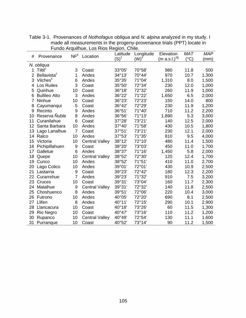
105
Table 3-1. Provenances of Nothofagus obliqua and N. alpina analyzed in my study. I
made all measurements in the progeny-provenance trials (PPT) locate in Fundo Arquilhue, Los Rios Region, Chile.
# Provenance NF£ Location Latitude (S)†
Longitude (W)†
Elevation (m a.s.l.)†§
MAT (°C)
MAP (mm)
N. obliqua
1 Tiltil¢ 3 Coast 33°05' 70°58' 980 11.8 500 2 Bellavista¢ 1 Andes 34°13' 70°44' 970 10.7 1,300 3 Vilches¢ 6 Andes 35°35' 71°04' 1,310 8.0 1,500 4 Los Ruiles 3 Coast 35°50' 72°34' 230 12.0 1,000 5 Quirihue 10 Coast 36°18' 72°32' 260 11.9 1,000 6 Bullileo Alto 3 Andes 36°22' 71°22' 1,650 6.5 2,000 7 Ninhue 10 Coast 36°23' 72°23' 150 14.0 800 8 Cayumanqui 5 Coast 36°42' 72°29' 230 11.9 1,200 9 Recinto 9 Andes 36°51' 71°40' 710 11.2 2,200
10 Reserva Ñuble 8 Andes 36°56' 71°13' 1,890 5.3 3,000 11 Curanilahue 6 Coast 37°28' 73°21' 140 12.5 2,000 12 Santa Barbara 10 Andes 37°40' 71°58' 430 10.5 1,800 13 Lago Lanalhue 7 Coast 37°51' 73°21' 230 12.1 2,000 14 Ralco 10 Andes 37°53' 71°35' 810 9.5 4,000 15 Victoria 10 Central Valley 38°12' 72°10' 480 11.4 1,500 16 Pichipillahuen 9 Coast 38°20' 73°03' 450 11.0 1,700 17 Galletue 6 Andes 38°37' 71°16' 1,450 5.8 2,000 18 Quepe 10 Central Valley 38°52' 72°30' 120 12.4 1,700 19 Cunco 10 Andes 38°52' 71°51' 410 11.0 2,700 20 Lago Colico 10 Andes 39°01' 72°01' 430 10.9 2,500 21 Lastarria 9 Coast 39°23' 72°42' 180 12.3 2,200 22 Curarrehue 7 Andes 39°23' 71°32' 910 7.5 3,200 23 Cruces 10 Coast 39°31' 73°04' 160 11.7 2,300 24 Malalhue 9 Central Valley 39°31' 72°32' 140 11.8 2,500 25 Choshuenco 8 Andes 39°51' 72°06' 220 10.4 3,000 26 Futrono 10 Andes 40°05' 72°20' 690 8.1 2,500 27 Llifen 8 Andes 40°11' 72°15' 290 10.1 2,900 28 Llancacura 10 Coast 40°18' 73°26' 60 11.5 1,300 29 Rio Negro 10 Coast 40°47' 73°16' 110 11.2 1,200 30 Rupanco 10 Central Valley 40°49' 72°54' 130 11.1 1,600 31 Purranque 10 Coast 40°52' 73°14' 90 11.2 1,500
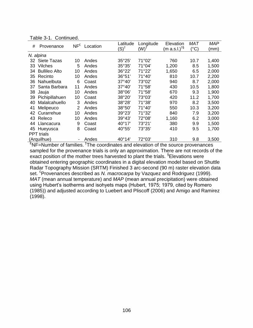
106
Table 3-1. Continued.
# Provenance NF£ Location Latitude (S)†
Longitude (W)†
Elevation (m a.s.l.)†§
MAT (°C)
MAP (mm)
N. alpina
32 Siete Tazas 10 Andes 35°25' 71°02' 760 10.7 1,400 33 Vilches 5 Andes 35°35' 71°04' 1,200 8.5 1,500 34 Bullileo Alto 10 Andes 36°22' 71°22' 1,650 6.5 2,000 35 Recinto 10 Andes 36°51' 71°40' 810 10.7 2,200 36 Nahuelbuta 6 Coast 37°40' 73°02' 940 8.7 2,000 37 Santa Barbara 11 Andes 37°40' 71°58' 430 10.5 1,800 38 Jauja 10 Andes 38°06' 71°58' 670 9.3 1,900 39 Pichipillahuen 10 Coast 38°20' 73°03' 420 11.2 1,700 40 Malalcahuello 3 Andes 38°28' 71°38' 970 8.2 3,500 41 Melipeuco 2 Andes 38°50' 71°40' 550 10.3 3,200 42 Curarrehue 10 Andes 39°23' 71°32' 840 7.9 3,200 43 Releco 10 Andes 39°43' 72°08' 1,160 6.2 3,000 44 Llancacura 9 Coast 40°17' 73°21' 380 9.9 1,500 45 Hueyusca 8 Coast 40°55' 73°35' 410 9.5 1,700 PPT trials (Arquilhue) - Andes 40°14' 72°03' 310 9.8 3,500 £NF=Number of families. †The coordinates and elevation of the source provenances sampled for the provenance trials is only an approximation. There are not records of the exact position of the mother trees harvested to plant the trials. §Elevations were obtained entering geographic coordinates in a digital elevation model based on Shuttle Radar Topography Mission (SRTM) Finished 3 arc-second (90 m) raster elevation data set. ¢Provenances described as N. macrocarpa by Vazquez and Rodriguez (1999). MAT (mean annual temperature) and MAP (mean annual precipitation) were obtained using Hubert‟s isotherms and isohyets maps (Hubert, 1975; 1979, cited by Romero (1985)) and adjusted according to Luebert and Pliscoff (2006) and Amigo and Ramirez (1998).
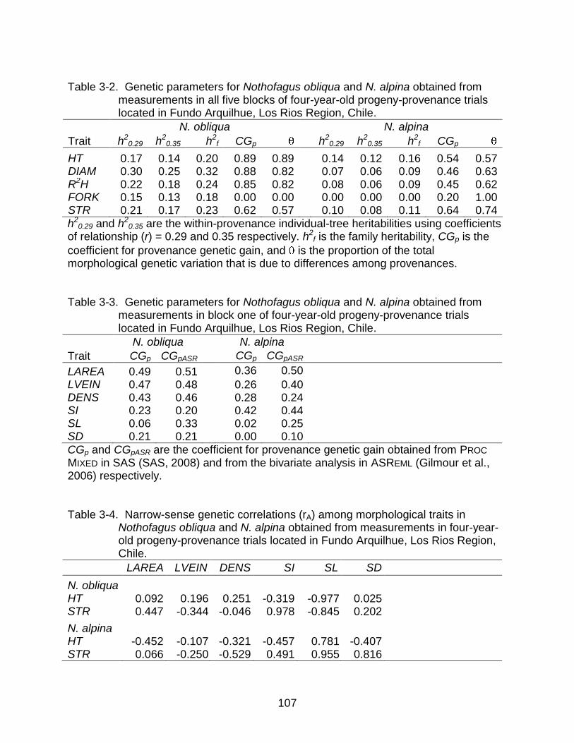
107
Table 3-2. Genetic parameters for Nothofagus obliqua and N. alpina obtained from
measurements in all five blocks of four-year-old progeny-provenance trials located in Fundo Arquilhue, Los Rios Region, Chile.
Trait
N. obliqua N. alpina
h20.29 h2
0.35 h2f CGp h2
0.29 h20.35 h2
f CGp
HT 0.17 0.14 0.20 0.89 0.89 0.14 0.12 0.16 0.54 0.57 DIAM 0.30 0.25 0.32 0.88 0.82 0.07 0.06 0.09 0.46 0.63 R2H 0.22 0.18 0.24 0.85 0.82 0.08 0.06 0.09 0.45 0.62 FORK 0.15 0.13 0.18 0.00 0.00 0.00 0.00 0.00 0.20 1.00 STR 0.21 0.17 0.23 0.62 0.57 0.10 0.08 0.11 0.64 0.74
h20.29 and h2
0.35 are the within-provenance individual-tree heritabilities using coefficients of relationship (r) = 0.29 and 0.35 respectively. h2
f is the family heritability, CGp is the
coefficient for provenance genetic gain, and is the proportion of the total morphological genetic variation that is due to differences among provenances. Table 3-3. Genetic parameters for Nothofagus obliqua and N. alpina obtained from
measurements in block one of four-year-old progeny-provenance trials located in Fundo Arquilhue, Los Rios Region, Chile.
Trait
N. obliqua N. alpina
CGp CGpASR CGp CGpASR
LAREA 0.49 0.51 0.36 0.50
LVEIN 0.47 0.48 0.26 0.40 DENS 0.43 0.46 0.28 0.24 SI 0.23 0.20 0.42 0.44 SL 0.06 0.33 0.02 0.25 SD 0.21 0.21 0.00 0.10
CGp and CGpASR are the coefficient for provenance genetic gain obtained from PROC
MIXED in SAS (SAS, 2008) and from the bivariate analysis in ASREML (Gilmour et al., 2006) respectively. Table 3-4. Narrow-sense genetic correlations (rA) among morphological traits in
Nothofagus obliqua and N. alpina obtained from measurements in four-year-old progeny-provenance trials located in Fundo Arquilhue, Los Rios Region, Chile.
LAREA LVEIN DENS SI SL SD
N. obliqua
HT 0.092 0.196 0.251 -0.319 -0.977 0.025 STR 0.447 -0.344 -0.046 0.978 -0.845 0.202
N. alpina
HT -0.452 -0.107 -0.321 -0.457 0.781 -0.407 STR 0.066 -0.250 -0.529 0.491 0.955 0.816
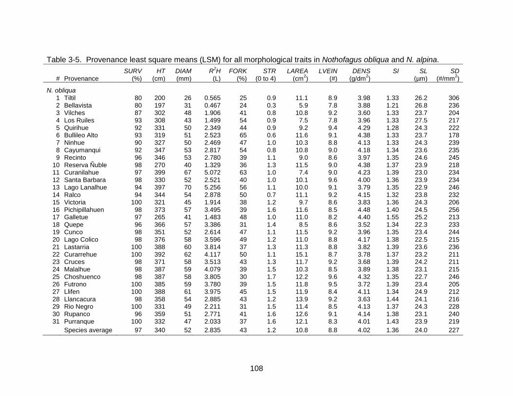
108
Table 3-5. Provenance least square means (LSM) for all morphological traits in Nothofagus obliqua and N. alpina.
# Provenance SURV
(%) HT
(cm) DIAM (mm)
R2H
(L) FORK
(%) STR
(0 to 4) LAREA
(cm2)
LVEIN (#)
DENS (g/dm
2)
SI
SL (µm)
SD (#/mm
2)
N. obliqua 1 Tiltil 80 200 26 0.565 25 0.9 11.1 8.9 3.98 1.33 26.2 306 2 Bellavista 80 197 31 0.467 24 0.3 5.9 7.8 3.88 1.21 26.8 236 3 Vilches 87 302 48 1.906 41 0.8 10.8 9.2 3.60 1.33 23.7 204 4 Los Ruiles 93 308 43 1.499 54 0.9 7.5 7.8 3.96 1.33 27.5 217 5 Quirihue 92 331 50 2.349 44 0.9 9.2 9.4 4.29 1.28 24.3 222 6 Bullileo Alto 93 319 51 2.523 65 0.6 11.6 9.1 4.38 1.33 23.7 178 7 Ninhue 90 327 50 2.469 47 1.0 10.3 8.8 4.13 1.33 24.3 239 8 Cayumanqui 92 347 53 2.817 54 0.8 10.8 9.0 4.18 1.34 23.6 235 9 Recinto 96 346 53 2.780 39 1.1 9.0 8.6 3.97 1.35 24.6 245
10 Reserva Ñuble 98 270 40 1.329 36 1.3 11.5 9.0 4.38 1.37 23.9 218 11 Curanilahue 97 399 67 5.072 63 1.0 7.4 9.0 4.23 1.39 23.0 234 12 Santa Barbara 98 330 52 2.521 40 1.0 10.1 9.6 4.00 1.36 23.9 234 13 Lago Lanalhue 94 397 70 5.256 56 1.1 10.0 9.1 3.79 1.35 22.9 246 14 Ralco 94 344 54 2.878 50 0.7 11.1 9.2 4.15 1.32 23.8 232 15 Victoria 100 321 45 1.914 38 1.2 9.7 8.6 3.83 1.36 24.3 206 16 Pichipillahuen 98 373 57 3.495 39 1.6 11.6 8.5 4.48 1.40 24.5 256 17 Galletue 97 265 41 1.483 48 1.0 11.0 8.2 4.40 1.55 25.2 213 18 Quepe 96 366 57 3.386 31 1.4 8.5 8.6 3.52 1.34 22.3 233 19 Cunco 98 351 52 2.614 47 1.1 11.5 9.2 3.96 1.35 23.4 244 20 Lago Colico 98 376 58 3.596 49 1.2 11.0 8.8 4.17 1.38 22.5 215 21 Lastarria 100 388 60 3.814 37 1.3 11.3 8.8 3.82 1.39 23.6 236 22 Curarrehue 100 392 62 4.117 50 1.1 15.1 8.7 3.78 1.37 23.2 211 23 Cruces 98 371 58 3.513 43 1.3 11.7 9.2 3.68 1.39 24.2 211 24 Malalhue 98 387 59 4.079 39 1.5 10.3 8.5 3.89 1.38 23.1 215 25 Choshuenco 98 387 58 3.805 30 1.7 12.2 9.6 4.32 1.35 22.7 246 26 Futrono 100 385 59 3.780 39 1.5 11.8 9.5 3.72 1.39 23.4 205 27 Llifen 100 388 61 3.975 45 1.5 11.9 8.4 4.11 1.34 24.9 212 28 Llancacura 98 358 54 2.885 43 1.2 13.9 9.2 3.63 1.44 24.1 216 29 Rio Negro 100 331 49 2.211 31 1.5 11.4 8.5 4.13 1.37 24.3 228 30 Rupanco 96 359 51 2.771 41 1.6 12.6 9.1 4.14 1.38 23.1 240 31 Purranque 100 332 47 2.033 37 1.6 12.1 8.3 4.01 1.43 23.9 219
Species average 97 340 52 2.835 43 1.2 10.8 8.8 4.02 1.36 24.0 227
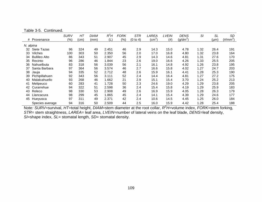
109
Table 3-5. Continued.
# Provenance SURV
(%) HT
(cm) DIAM (mm)
R2H
(L) FORK
(%) STR
(0 to 4) LAREA
(cm2)
LVEIN (#)
DENS (g/dm
2)
SI
SL (µm)
SD (#/mm
2)
N. alpina
32 Siete Tazas 96 324 49 2.451 46 2.9 14.3 15.0 4.78 1.32 26.4 191 33 Vilches 100 303 50 2.350 56 2.0 17.0 16.8 4.80 1.32 23.8 164 34 Bullileo Alto 86 343 51 2.907 45 2.9 14.3 14.6 4.81 1.31 27.6 170 35 Recinto 96 286 46 1.844 23 2.6 19.0 16.6 4.26 1.33 25.5 205 36 Nahuelbuta 83 318 56 3.039 56 2.1 16.1 14.8 4.92 1.26 23.8 195 37 Santa Barbara 97 364 56 3.574 46 2.7 16.6 15.8 4.02 1.27 24.7 203 38 Jauja 94 335 52 2.712 48 2.6 15.9 16.1 4.41 1.28 25.3 190 39 Pichipillahuen 92 343 56 3.111 52 2.4 14.4 16.4 4.81 1.27 27.2 175 40 Malalcahuello 93 268 46 1.662 21 2.9 15.1 15.4 3.70 1.24 25.2 213 41 Melipeuco 60 283 41 1.728 50 2.3 24.6 19.0 4.29 1.29 23.8 205 42 Curarrehue 94 322 51 2.598 36 2.4 15.4 15.8 4.19 1.29 25.9 183 43 Releco 98 330 53 2.908 49 2.6 16.9 15.9 4.05 1.28 26.3 179 44 Llancacura 98 299 45 1.865 45 2.4 14.1 15.4 4.39 1.29 24.6 177 45 Hueyusca 97 311 49 2.371 42 2.4 10.6 14.5 4.45 1.25 26.0 184
Species average 94 316 50 2.509 44 2.5 16.0 15.9 4.42 1.28 25.4 188
Note: SURV=survival, HT=total height, DIAM=stem diameter at the root collar, R2H=volume index, FORK=stem forking, STR= stem straightness, LAREA= leaf area, LVEIN=number of lateral veins on the leaf blade, DENS=leaf density, SI=shape index, SL= stomatal length, SD= stomatal density.
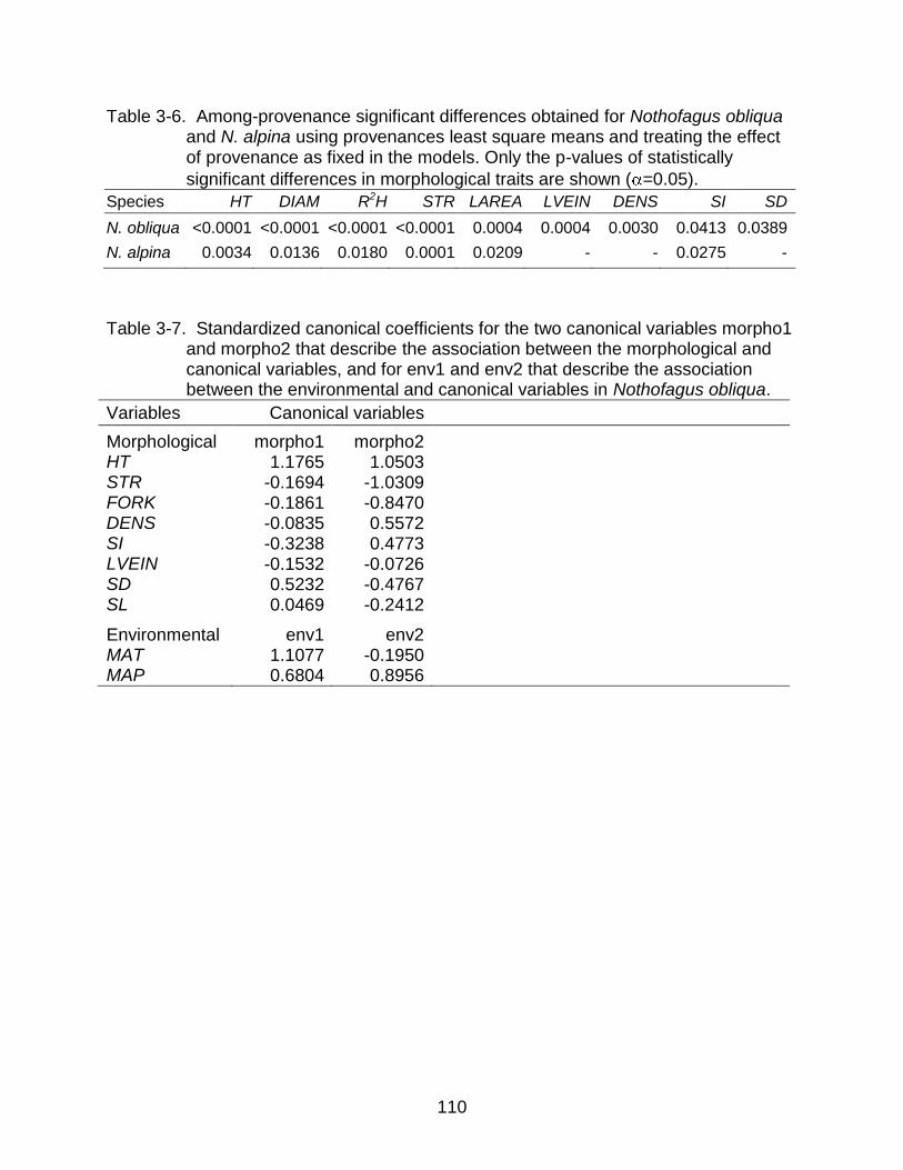
110
Table 3-6. Among-provenance significant differences obtained for Nothofagus obliqua and N. alpina using provenances least square means and treating the effect of provenance as fixed in the models. Only the p-values of statistically
significant differences in morphological traits are shown ( =0.05).
Species HT DIAM R2H STR LAREA LVEIN DENS SI SD
N. obliqua <0.0001 <0.0001 <0.0001 <0.0001 0.0004 0.0004 0.0030 0.0413 0.0389
N. alpina 0.0034 0.0136 0.0180 0.0001 0.0209 - - 0.0275 -
Table 3-7. Standardized canonical coefficients for the two canonical variables morpho1 and morpho2 that describe the association between the morphological and canonical variables, and for env1 and env2 that describe the association between the environmental and canonical variables in Nothofagus obliqua.
Variables Canonical variables
Morphological morpho1 morpho2
HT 1.1765 1.0503 STR -0.1694 -1.0309 FORK -0.1861 -0.8470 DENS -0.0835 0.5572 SI -0.3238 0.4773 LVEIN -0.1532 -0.0726 SD 0.5232 -0.4767 SL 0.0469 -0.2412
Environmental env1 env2 MAT 1.1077 -0.1950 MAP 0.6804 0.8956
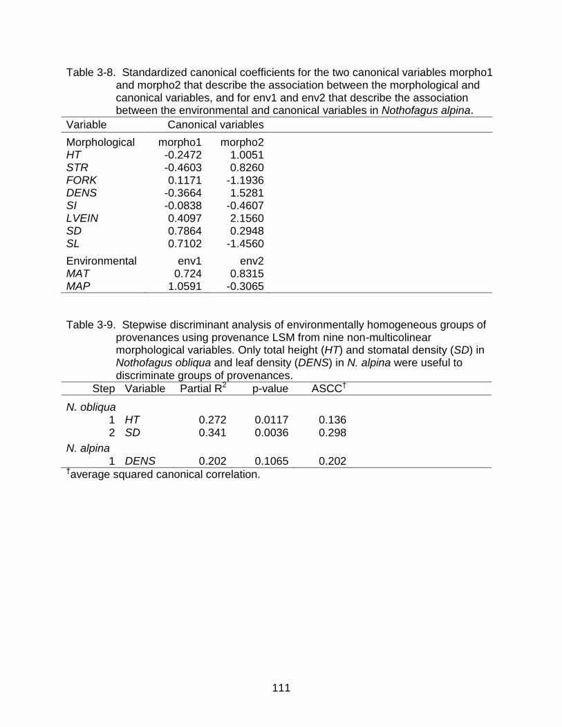
111
Table 3-8. Standardized canonical coefficients for the two canonical variables morpho1 and morpho2 that describe the association between the morphological and canonical variables, and for env1 and env2 that describe the association between the environmental and canonical variables in Nothofagus alpina.
Variable Canonical variables
Morphological morpho1 morpho2
HT -0.2472 1.0051 STR -0.4603 0.8260 FORK 0.1171 -1.1936 DENS -0.3664 1.5281 SI -0.0838 -0.4607 LVEIN 0.4097 2.1560 SD 0.7864 0.2948 SL 0.7102 -1.4560
Environmental env1 env2
MAT 0.724 0.8315 MAP 1.0591 -0.3065
Table 3-9. Stepwise discriminant analysis of environmentally homogeneous groups of
provenances using provenance LSM from nine non-multicolinear morphological variables. Only total height (HT) and stomatal density (SD) in Nothofagus obliqua and leaf density (DENS) in N. alpina were useful to discriminate groups of provenances.
Step Variable Partial R2 p-value ASCC†
N. obliqua 1 HT 0.272 0.0117 0.136 2 SD 0.341 0.0036 0.298
N. alpina
1 DENS 0.202 0.1065 0.202 †average squared canonical correlation.
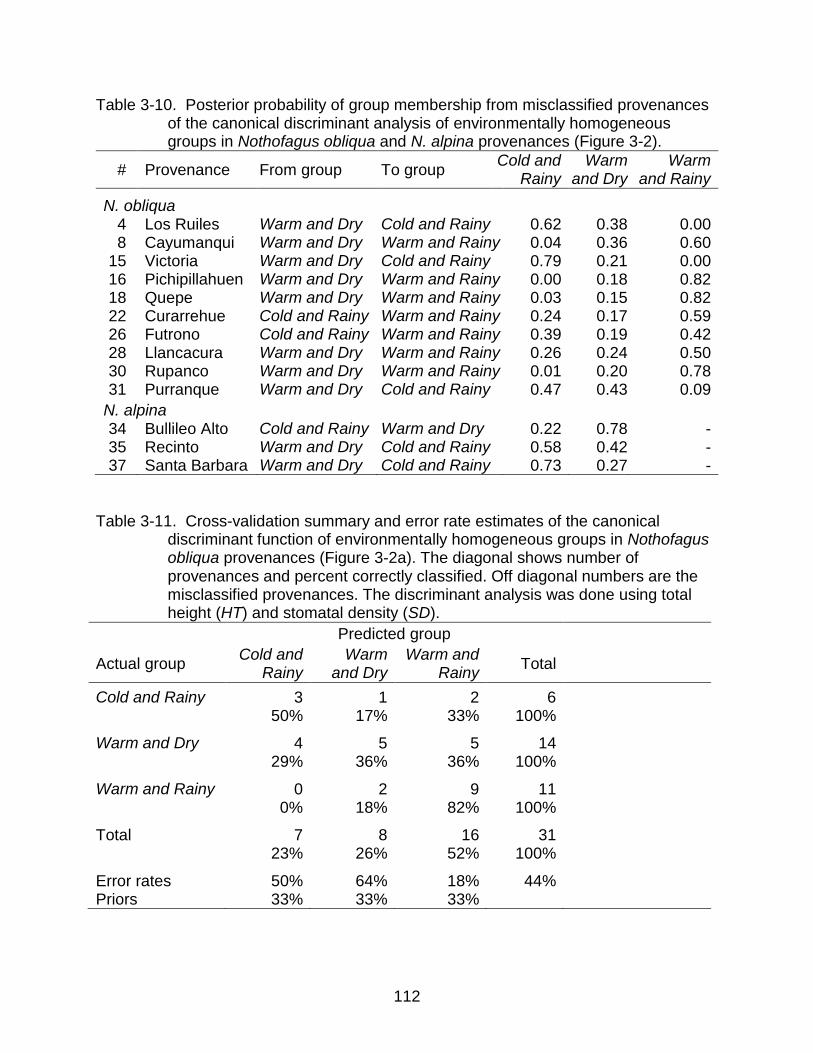
112
Table 3-10. Posterior probability of group membership from misclassified provenances of the canonical discriminant analysis of environmentally homogeneous groups in Nothofagus obliqua and N. alpina provenances (Figure 3-2).
# Provenance From group To group Cold and
Rainy Warm
and Dry Warm
and Rainy
N. obliqua 4 Los Ruiles Warm and Dry Cold and Rainy 0.62 0.38 0.00 8 Cayumanqui Warm and Dry Warm and Rainy 0.04 0.36 0.60
15 Victoria Warm and Dry Cold and Rainy 0.79 0.21 0.00 16 Pichipillahuen Warm and Dry Warm and Rainy 0.00 0.18 0.82 18 Quepe Warm and Dry Warm and Rainy 0.03 0.15 0.82 22 Curarrehue Cold and Rainy Warm and Rainy 0.24 0.17 0.59 26 Futrono Cold and Rainy Warm and Rainy 0.39 0.19 0.42 28 Llancacura Warm and Dry Warm and Rainy 0.26 0.24 0.50 30 Rupanco Warm and Dry Warm and Rainy 0.01 0.20 0.78 31 Purranque Warm and Dry Cold and Rainy 0.47 0.43 0.09
N. alpina
34 Bullileo Alto Cold and Rainy Warm and Dry 0.22 0.78 - 35 Recinto Warm and Dry Cold and Rainy 0.58 0.42 - 37 Santa Barbara Warm and Dry Cold and Rainy 0.73 0.27 -
Table 3-11. Cross-validation summary and error rate estimates of the canonical
discriminant function of environmentally homogeneous groups in Nothofagus obliqua provenances (Figure 3-2a). The diagonal shows number of provenances and percent correctly classified. Off diagonal numbers are the misclassified provenances. The discriminant analysis was done using total height (HT) and stomatal density (SD).
Predicted group
Actual group Cold and
Rainy Warm
and Dry Warm and
Rainy Total
Cold and Rainy 3 1 2 6
50% 17% 33% 100%
Warm and Dry 4 5 5 14 29% 36% 36% 100%
Warm and Rainy 0 2 9 11 0% 18% 82% 100%
Total 7 8 16 31 23% 26% 52% 100%
Error rates 50% 64% 18% 44% Priors 33% 33% 33%
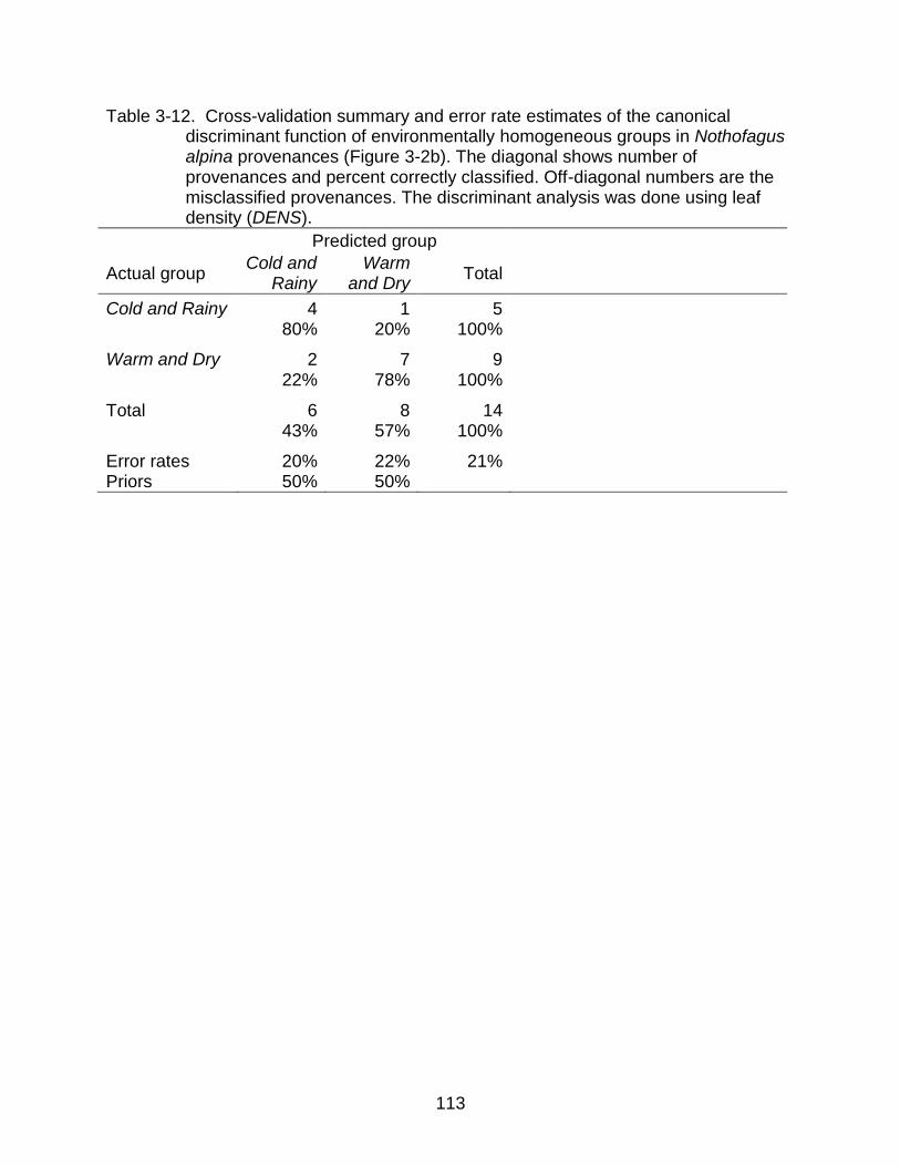
113
Table 3-12. Cross-validation summary and error rate estimates of the canonical discriminant function of environmentally homogeneous groups in Nothofagus alpina provenances (Figure 3-2b). The diagonal shows number of provenances and percent correctly classified. Off-diagonal numbers are the misclassified provenances. The discriminant analysis was done using leaf density (DENS).
Predicted group
Actual group Cold and
Rainy Warm
and Dry Total
Cold and Rainy 4 1 5
80% 20% 100%
Warm and Dry 2 7 9 22% 78% 100%
Total 6 8 14 43% 57% 100%
Error rates 20% 22% 21% Priors 50% 50%
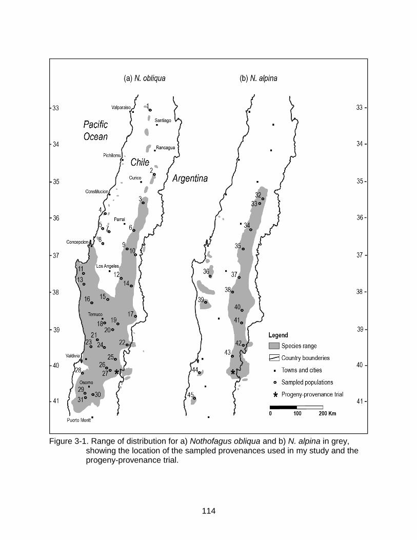
114
Figure 3-1. Range of distribution for a) Nothofagus obliqua and b) N. alpina in grey, showing the location of the sampled provenances used in my study and the progeny-provenance trial.
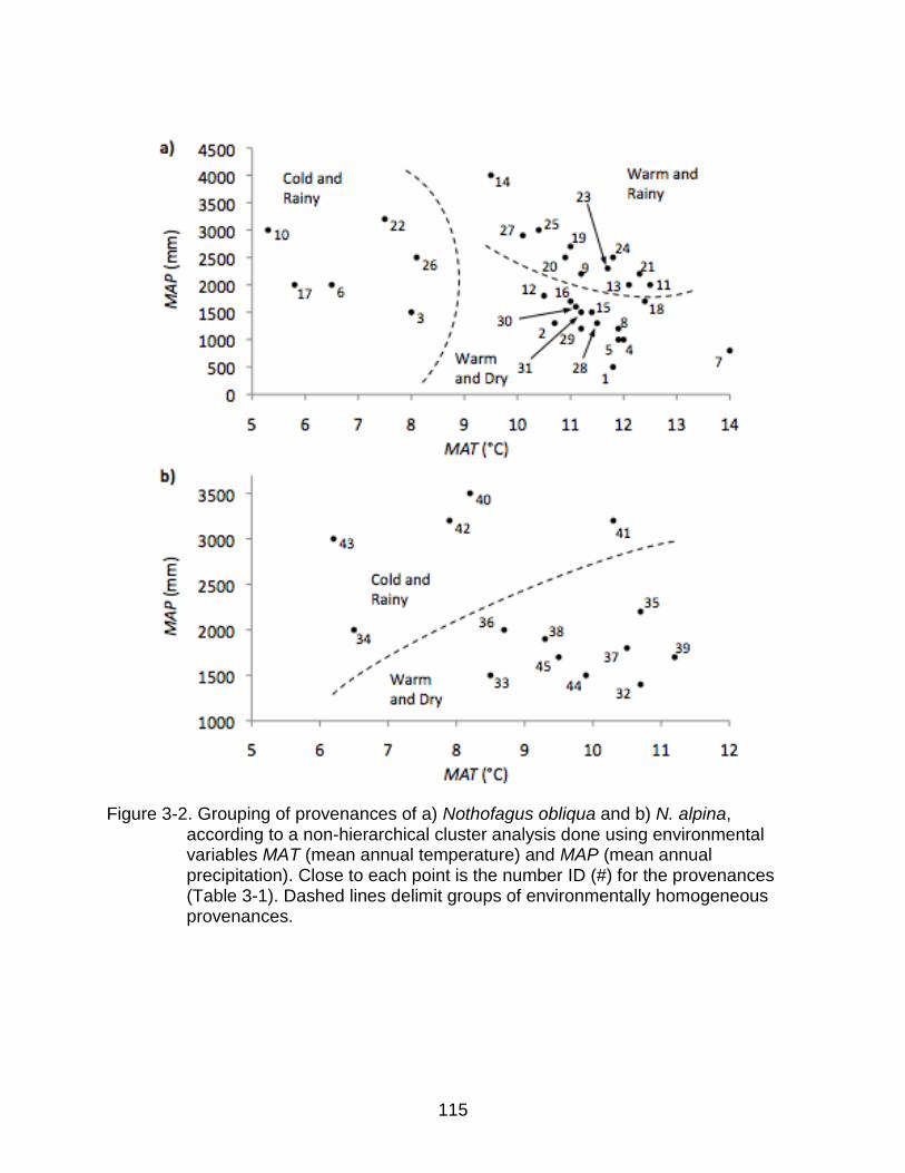
115
Figure 3-2. Grouping of provenances of a) Nothofagus obliqua and b) N. alpina, according to a non-hierarchical cluster analysis done using environmental variables MAT (mean annual temperature) and MAP (mean annual precipitation). Close to each point is the number ID (#) for the provenances (Table 3-1). Dashed lines delimit groups of environmentally homogeneous provenances.
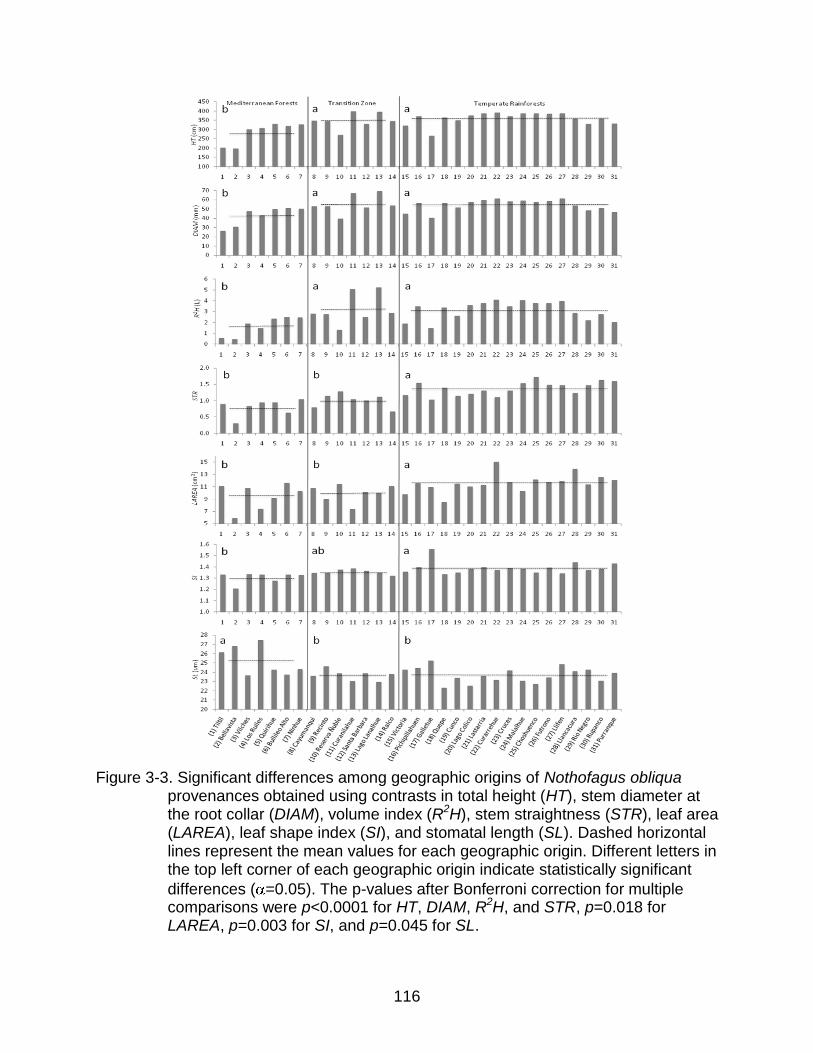
116
Figure 3-3. Significant differences among geographic origins of Nothofagus obliqua
provenances obtained using contrasts in total height (HT), stem diameter at the root collar (DIAM), volume index (R2H), stem straightness (STR), leaf area (LAREA), leaf shape index (SI), and stomatal length (SL). Dashed horizontal lines represent the mean values for each geographic origin. Different letters in the top left corner of each geographic origin indicate statistically significant
differences ( =0.05). The p-values after Bonferroni correction for multiple comparisons were p<0.0001 for HT, DIAM, R2H, and STR, p=0.018 for LAREA, p=0.003 for SI, and p=0.045 for SL.
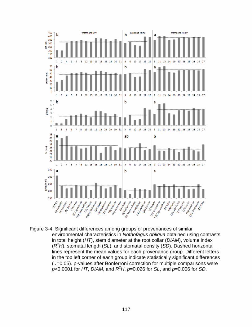
117
Figure 3-4. Significant differences among groups of provenances of similar environmental characteristics in Nothofagus obliqua obtained using contrasts in total height (HT), stem diameter at the root collar (DIAM), volume index (R2H), stomatal length (SL), and stomatal density (SD). Dashed horizontal lines represent the mean values for each provenance group. Different letters in the top left corner of each group indicate statistically significant differences
( =0.05). p-values after Bonferroni correction for multiple comparisons were p<0.0001 for HT, DIAM, and R2H, p=0.026 for SL, and p=0.006 for SD.
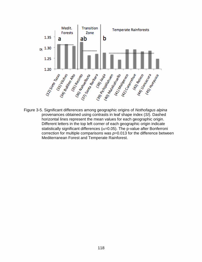
118
Figure 3-5. Significant differences among geographic origins of Nothofagus alpina
provenances obtained using contrasts in leaf shape index (SI). Dashed horizontal lines represent the mean values for each geographic origin. Different letters in the top left corner of each geographic origin indicate
statistically significant differences ( =0.05). The p-value after Bonferroni correction for multiple comparisons was p=0.013 for the difference between Mediterranean Forest and Temperate Rainforest.
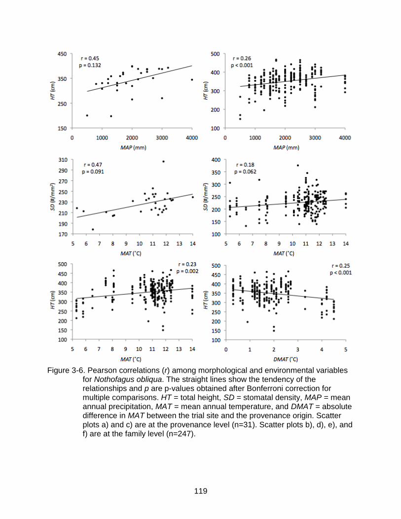
119
Figure 3-6. Pearson correlations (r) among morphological and environmental variables
for Nothofagus obliqua. The straight lines show the tendency of the relationships and p are p-values obtained after Bonferroni correction for multiple comparisons. HT = total height, SD = stomatal density, MAP = mean annual precipitation, MAT = mean annual temperature, and DMAT = absolute difference in MAT between the trial site and the provenance origin. Scatter plots a) and c) are at the provenance level (n=31). Scatter plots b), d), e), and f) are at the family level (n=247).
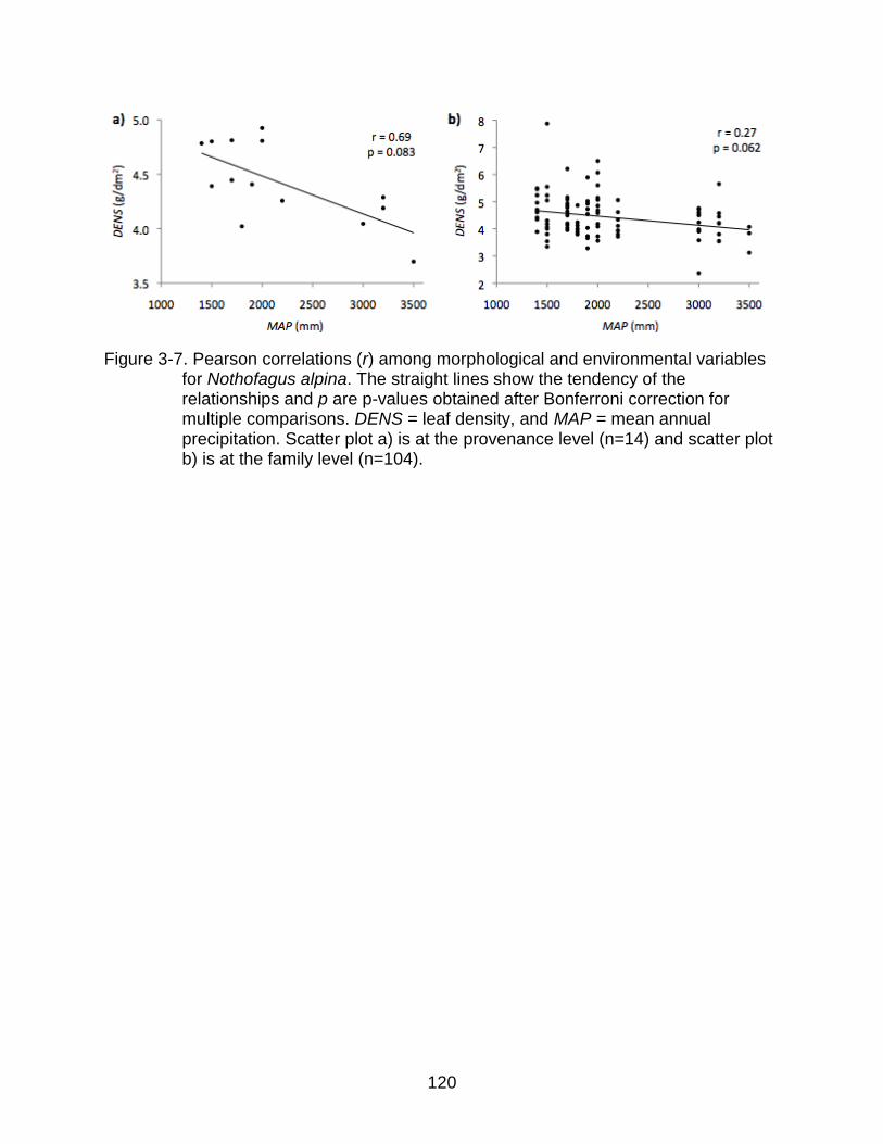
120
Figure 3-7. Pearson correlations (r) among morphological and environmental variables for Nothofagus alpina. The straight lines show the tendency of the relationships and p are p-values obtained after Bonferroni correction for multiple comparisons. DENS = leaf density, and MAP = mean annual precipitation. Scatter plot a) is at the provenance level (n=14) and scatter plot b) is at the family level (n=104).
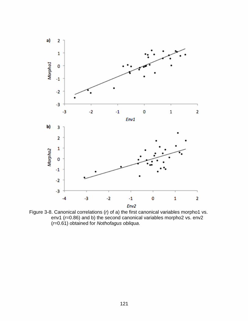
121
Figure 3-8. Canonical correlations (r) of a) the first canonical variables morpho1 vs.
env1 (r=0.86) and b) the second canonical variables morpho2 vs. env2 (r=0.61) obtained for Nothofagus obliqua.
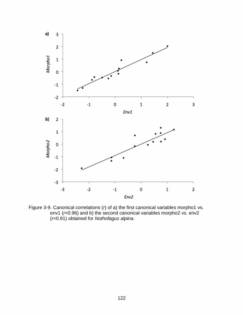
122
Figure 3-9. Canonical correlations (r) of a) the first canonical variables morpho1 vs. env1 (r=0.96) and b) the second canonical variables morpho2 vs. env2 (r=0.91) obtained for Nothofagus alpina.
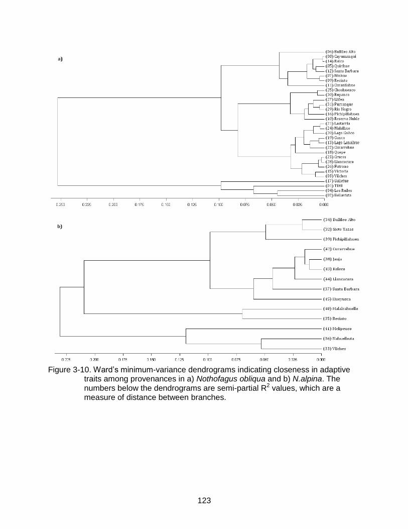
123
Figure 3-10. Ward‟s minimum-variance dendrograms indicating closeness in adaptive
traits among provenances in a) Nothofagus obliqua and b) N.alpina. The numbers below the dendrograms are semi-partial R2 values, which are a measure of distance between branches.
124
CHAPTER 4 SYSTEMATICS, CONSERVATION GENETICS, AND BREEDING ZONES DEFINITION
BASED ON NEUTRAL AND ADAPTIVE PATTERNS OF GENETIC VARIATION IN NOTHOFAGUS OBLIQUA, N. ALPINA, AND N. GLAUCA
Introductory Remarks
A sound approach to making decisions about the conservation and sustainable
use of a group of closely related species should include resolving the systematic
relationship among those species, assessing the potential and extent of hybridization,
and estimating their within-species variation structure considering both neutral and
adaptive genetic variation.
The genetic variation within and among species is often analyzed using neutral
molecular markers such as isozymes or an assortment of DNA markers. The use of
these techniques is relatively inexpensive and fast (McKay and Latta, 2002; van
Tienderen et al., 2002). Unfortunately, variability obtained from the analysis of neutral
markers has been shown to be uncorrelated with adaptive variability obtained from the
analysis of morphological markers (Reed and Frankham, 2001; McKay and Latta,
2002). Adaptive genetic variation is a very important component for conservation,
because whereas neutral variation determines the underlying potential for longer-term
evolutionary changes, adaptive variation determines the evolutionary potential to
respond to more immediate changes (McKay and Latta, 2002). Thus, the combined
analysis of neutral and adaptive markers is important for the development of
conservation and genetic improvement strategies of forest trees.
Nothofagus obliqua (Mirb.) Oerst., N. alpina (Poepp. et Endl.) Oerst. (= N.
nervosa), and N. glauca (Phil.) Krasser. make up the South American clade of
subgenus Lophozonia (Manos, 1997). These three species are sympatric, endemic, and
125
closely related, but the systematic relationships within the clade are not clear. There is a
combined consensus tree recovered by Manos (1997) showing a closer relationship
between N. alpina and N. glauca, leaving N. obliqua as the sister to their branch.
However, the moderate support for that topology (bootstrap=77%), the current
geographic range of the species (Figure 4-1), and the evidence that hybridization occurs
between N. obliqua and both N. alpina and N. glauca but not between the latter two
(Donoso, 1979; Donoso et al., 1990), suggests that N. alpina and N. glauca might not
be the most genetically similar species within the clade. In addition, Vazquez and
Rodriguez (1999) proposed a new species for the subgenus (N. macrocarpa (A.DC.)
F.M. Vazquez & R.A. Rodr., formerly N. obliqua var. macrocarpa A.DC.) and recognized
three subspecies of N. obliqua (ssp. obliqua (Mirb.) Oerst., spp. valdiviana (Phil.) F.M.
Vazquez & R.A. Rodr., and ssp. andina F.M. Vazquez & R.A. Rodr.), adding a new
element to the discussion.
The conservation status of these species overall is not critical. Nothofagus obliqua
and N. alpina have been classified as out of danger or near threatened and N. glauca
as vulnerable by Benoit (1989) and Gonzalez (1998a; 1998b). However, threats to
particular populations mainly in the northern area of distribution (33°00‟-36°30‟S), but
also in other localities across their range, are serious and may potentially lead to local
extinction. Besides, the populations of these species are poorly represented in the
Chilean National Wild Lands System (SNASPE). Overall, less than 6%, 8%, and 2% of
N. obliqua, N. alpina, and N. glauca, respectively, are within protected areas
(Ormazabal and Benoit, 1987).
126
The species of Lophozonia in South America are greatly valued because of their
high-quality wood and fast growth. Therefore, it is important to incorporate the use of
their wood in the conservation equation. There is evidence that their populations have
steadily degraded because of their commercial value, and the most desirable
phenotypes are gone (Vergara and Bohle, 2000). Thus, breeding programs leading to
genetic improvement of these tree species are needed to attempt the recovering of
genotypes that would maximize growth and wood quality and also general fitness to the
current and future environments. A tree improvement strategy should take into account,
among many elements, the genetic structure and variability of populations to assure the
conservation of within-population variability as well as regional genetic identities. The
tree improvement strategy proposed for the populations of N. obliqua and N. alpina
growing in Chile (Ipinza and Gutierrez, 2000) uses, as general guidance, regions of
provenance defined by Vergara (2000). However, this strategy only uses the regions of
provenance to prioritize the regions where the selection and genetic tests should be
done. It does not explicitly use the regions of provenance to organize the genetic
material in breeding zones mainly because of the lack, at the time, of neutral or adaptive
genetic information needed to characterize such regions.
The objectives of my study are to: 1) elucidate the systematics of the South
American clade of subgenus Lophozonia including their inter- and infraspecific genetic
similarities by using high-resolution nuclear microsatellite data for populations of the
three species (Chapter 2); 2) identify conservation priorities among the studied
populations and generate rankings that will take into account uniqueness and
complementarity of populations within each species by combining nuclear microsatellite
127
data (Chapter 2), morphological data obtained from common gardens (Chapter 3), and
maternally inherited chloroplast DNA data (Azpilicueta et al., 2009; Marchelli and Gallo,
2006); and 3) using the latter three sets of information, evaluate the relevance of
defining breeding zones in the tree improvement strategy for the species belonging to
Nothofagus subgenus Lophozonia.
Material and Methods
Sources of Data Used for the Analyses
The data I used in these analyses came from three sources that obtained genetic
information from the same seed lots in most of the populations (Table 4-1) and in some
cases, the same individuals. The first source included data from seven high-resolution
nuclear microsatellite loci (the nMSAT data set) obtained for 20 populations of
Nothofagus obliqua, 12 populations of N. alpina, and 8 populations of N. glauca
(Chapter 2). The second source consisted of morphological data from 14 adaptive traits
measured in common gardens (the ADAP data set) with a randomized complete block
design, representing open-pollinated families from 31 N. obliqua and 14 N. alpina
populations (Chapter 3). The third source comprised PCR-RFLP fragment data from
maternally inherited chloroplast DNA regions (the cpDNA data set) obtained from 27 N.
obliqua (Azpilicueta et al., 2009) and 26 N. alpina (Marchelli and Gallo, 2006)
populations. All three data sources covered most of the species ranges of distribution in
Chile (Figure 4-1).
Analysis of Genetic Similarities among Species
Bayesian analysis
To examine the genetic similarities among species, I used an individual-based
approach assuming no specific mutation model using Bayesian clustering in STRUCTURE
128
2.3.2 (Pritchard et al., 2000). Using the nMSAT data set, I analyzed all the populations
of the three species together with a total of 640 individuals from 40 populations. I used
the admixture model with correlated allele frequencies and without including population
information in the analyses as recommended by Falush et al. (2003). I ran STRUCTURE
at multiple K values (K=number of assumed clusters in the data) from K=1 to K=8. At
each K, I carried out 10 separate runs of 200,000 generations each with a burn-in of
100,000. I obtained posterior probabilities (LnP[D]) and computed Evanno‟s ΔK (Evanno
et al., 2005) to select the optimal K when LnP[D] turns asymptotic. I analyzed this data
set with the seven original nMSAT loci and also by eliminating locus ncutas04 because
it was only polymorphic in N. glauca (Chapter 2) and could bias the results. I employed
DISTRUCT 1.1 (Rosenberg, 2004) to visualize and edit the STRUCTURE outputs.
Pairwise genetic distances
Another way to examine the genetic similarity among species is by obtaining
pairwise genetic distances among the populations of all three species simultaneously.
Again, using the nMSAT data set and assuming a stepwise mutation model (SMM,
Slatkin, 1995), I ran ARLEQUIN 3.11 (Excoffier et al., 2005) to obtain a pairwise RST
matrix with 100 permutations to obtain significance, using standard Bonferroni
corrections on all pairwise differences (Rice, 1989). As in the Bayesian analysis, I ran
ARLEQUIN with and without locus ncutas04 to compare results. Pairwise RST are
measures of genetic differentiation among populations and were used to obtain
unrooted neighbor-joining (NJ) trees in PHYLIP 3.69 (Felsenstein, 1989), employing the
component NEIGHBOR to infer species similarities within the clade. I visualized the
resulting trees with TREEVIEW 1.6.6 (Page, 1996). Additionally, STRUCTURE 2.3.2
(Pritchard et al., 2000) also delivers NEIGHBOR/PHYLIP unrooted neighbor-joining trees
129
from allele-frequency divergence values assuming an infinite allele model (IAM) for K
pairs of STRUCTURE clusters. I used these trees to compare results among all methods.
Methods of Ranking Populations for Conservation
Rankings based on allelic richness
Allelic richness is a diversity parameter of high priority in conservation genetics
and is most useful when applied to highly variable markers like microsatellite DNA (Petit
et al., 1998). I used the approach of Petit et al. (1998) to obtain the relative conservation
value for each population within each species based on the marginal allelic richness
contributed by the populations to the total allelic richness of the species. Thus, the
populations were ranked according to their contribution to the total allelic richness (CT)
using:
CT (k) = (rT – rT\k) / (rT – 1) (4-1)
where
CT (k) = contribution of the kth population to the total allelic richness,
rT = estimator of the total allelic richness, and
rT\k = estimator of the total allelic richness when the kth population is excluded.
I obtained allelic richness estimations from the nMSAT and cpDNA data sets. To
input allelic richness values in the equation, I standardized them using rarefaction to
correct for uneven sample size (Kalinowski, 2004) using HP-RARE 1.1 (Kalinowski,
2005).
Rankings based on dendrograms
Other ranking options based on conservation value are given by systematics with
the assessment of taxonomic distinctness (Vane-Wright et al., 1991; Faith, 1994). The
various systematics approaches developed to obtain conservation values are intended
130
to give greater conservation weight to taxa that are unique and although they were
designed to define conservation priorities among different species and groups of
species, I applied them to rank populations within species based on the nMSAT and
ADAP dendrograms obtained in Chapter 2 and Chapter 3, respectively.
I utilized the root weighting procedure developed by Vane-Wright et al. (1991)
including May‟s modifications (May, 1990) to prioritize populations for conservation
based on topology and without directly considering genetic distances among
populations. For each population in a dendrogram I traced all the nodes to the “base” of
the dendrogram counting all the branches at each node. The populations were then
ranked obtaining the percentage contribution for each population to the total diversity
(PT) with:
PT (k) = 100[(bT / bk) / ∑ (bT / bk)] (4-2)
where
PT (k) = percentage contribution of the kth population to the total diversity,
bT = total branch count adding all populations, and
bk = total branch count for the kth population.
Results
Among-Species Genetic Similarity Inferred from Bayesian Clustering
The analysis in STRUCTURE grouping all forty populations from the three species
together produced log posterior probabilities (LnP[D]) for K=1 to K=8. Figure 4-2 shows
the curves of LnP[D] and Evanno‟s ΔK (Evanno et al., 2005) defining a peak to find the
optimal number of clusters (K). The higher ΔK values in K=3 obtained for both
analyses–that with all seven loci and that with the six polymorphic loci–indicated a
131
strong signal to identify three clusters coinciding with the species boundaries defined in
my study (Figure 4-3a and b).
I also show the results for K=2 and K=4 because, although suboptimal, they give
an idea of the among-species similarities (K=2) and of putative within-species
differentiation (K=4) in this South American clade. In this case, results are quite different
between the two analyses. For K=2 and using the seven loci (Figure 4-3a), Nothofagus
obliqua clearly clustered with N. alpina leaving N. glauca in its own cluster. However,
using only the six polymorphic loci (Figure 4-3b), N. obliqua clustered with N. glauca
instead. Also, for K=4 and using the seven loci (Figure 4-3a), N. obliqua was subdivided
into two groups, with populations from the Mediterranean Forest (33°00‟-36°20‟S)
separated from the Transitional Forests and Termperate Rainforests populations south
of 36°20‟S (Figure 4-1). When using only the six polymorphic loci (Figure 4-3b), the limit
between the two groups in N. obliqua changed and now most of the populations from
the Mediterranean and Transitional Forests (33°00‟-38°20‟S) cluster together and apart
from the Temperate Rainforests populations (Figure 4-1).
Among-Species Genetic Similarities Inferred from Pairwise Genetic Distances
I obtained two unrooted NJ trees using pairwise RST matrices for all pairs of
populations combined, one using all seven available loci (Figure 4-4a) and another
using the six polymorphic loci (Figure 4-4b). Both trees show three clearly defined
groups matching the three species analyzed. Almost all populations fell well within each
group with the sole exception of Loncha (5) from N. obliqua, which seems to be apart
from every population with a slight tendency to the N. glauca branch. These two trees
do not show a trend of similarity among species or of geographic within-species
differentiation. Coastal populations Pichipillahuen (26) and Cruces (36) from N. obliqua
132
cluster very close to each other and apart from all the other populations in the species.
However, this similarity does not make sense geographically (Figure 4-1).
As another way to observe among-species similarities and possible geographic
within-species differentiation, I obtained four unrooted NJ trees assuming the infinite
allele model (IAM) among K=3 and K=4 pairs of population clusters from the STRUCTURE
analyses. For each K, I obtained one tree using all seven available loci (Figure 4-4c)
and another using the six polymorphic loci (Figure 4-4d). Results show a greater
similatiry of N. obliqua with N. alpina rather than with N. glauca and little evidence of
within-species differentiation in N. obliqua across all four dendrograms.
Ranking for Conservation Using Population’s Contribution to Total Allelic Richness
I obtained the contribution to total allelic richness (CT) for nuclear markers (nMSAT
data set) in 20 N. obliqua, 12 N. alpina, and 8 N. glauca populations (Figure 4-5), and
for chloroplast markers (cpDNA data set) in 27 N. obliqua and 26 N. alpina populations.
Of these, 11 N. obliqua and 8 N. alpina populations are common to both data sets or
are different samples of the same population (Table 4-1). Table 4-1 shows the within-
species conservation rankings (rnk CT) for the contribution to CT in both data sets and
highlights approximately the top 25% populations for each species/marker combination.
Of the 19 populations common to both data sets, eight belonged to the top 25% in just
one marker and only Nahuelbuta (54) and Pichipillahuen (57) in N. alpina were ranked
top 25% for both sets of markers.
Ranking for Conservation Using Population Genetic Distinctness
Using dendrograms based on among-population genetic similarities, I calculated
the percentage contribution to total diversity (PT) of each population based on
133
population distinctness for nuclear markers (nMSAT data set) in 20 N. obliqua, 12 N.
alpina, and 8 N. glauca populations (Figure 4-5), and for adaptive markers (ADAP data
set) in 31 N. obliqua and 14 N. alpina populations (Figure 4-6). In this case, 18 N.
obliqua and 11 N. alpina populations are common for both data sets or are different
samples of the same population (Table 4-1). Figures 4-5 and 4-6 show the PT values
and their respective within-species conservation rankings in which it is important to note
that the approximately top 25% ranked populations account for about 50 to 60% of the
total diversity in each species/marker combination. Also Table 4-1 shows the within-
species conservation rankings (rnk PT) based on PT values in both data sets and
highlights approximately the top 25% populations for each species/marker combination.
Of the 29 populations common to both markers, eight belonged to the top 25% in just
one marker, and only La Campana/Tiltil (1/2), Sierras de Bellavista/Bellavista (7/8), and
Galletue (27) in N. obliqua were ranked top 25% for both markers.
Discussion
Genetic Similarities among Species
The two major questions about the systematic relationships in the South American
clade of subgenus Lophozonia relate to the topology among the three species and to
the subdivision of Nothofagus obliqua in two sister species and other subspecies.
Manos (1997), with his combined consensus tree obtained analyzing ITS
sequences, plastid sequences, and morphology, placed N. alpina and N. glauca in a
clade and N. obliqua as their sister species. My results analyzing seven highly variable
nuclear microsatellite loci did not agree with this topology and favored greater similarity
between N. obliqua and N. alpina, with N. glauca more genetically distant in both the
STRUCTURE analysis (Figure 4-3a) and the neighbor-joining (NJ) trees obtained
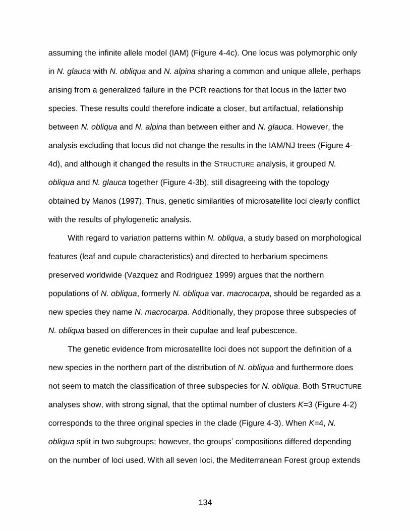
134
assuming the infinite allele model (IAM) (Figure 4-4c). One locus was polymorphic only
in N. glauca with N. obliqua and N. alpina sharing a common and unique allele, perhaps
arising from a generalized failure in the PCR reactions for that locus in the latter two
species. These results could therefore indicate a closer, but artifactual, relationship
between N. obliqua and N. alpina than between either and N. glauca. However, the
analysis excluding that locus did not change the results in the IAM/NJ trees (Figure 4-
4d), and although it changed the results in the STRUCTURE analysis, it grouped N.
obliqua and N. glauca together (Figure 4-3b), still disagreeing with the topology
obtained by Manos (1997). Thus, genetic similarities of microsatellite loci clearly conflict
with the results of phylogenetic analysis.
With regard to variation patterns within N. obliqua, a study based on morphological
features (leaf and cupule characteristics) and directed to herbarium specimens
preserved worldwide (Vazquez and Rodriguez 1999) argues that the northern
populations of N. obliqua, formerly N. obliqua var. macrocarpa, should be regarded as a
new species they name N. macrocarpa. Additionally, they propose three subspecies of
N. obliqua based on differences in their cupulae and leaf pubescence.
The genetic evidence from microsatellite loci does not support the definition of a
new species in the northern part of the distribution of N. obliqua and furthermore does
not seem to match the classification of three subspecies for N. obliqua. Both STRUCTURE
analyses show, with strong signal, that the optimal number of clusters K=3 (Figure 4-2)
corresponds to the three original species in the clade (Figure 4-3). When K=4, N.
obliqua split in two subgroups; however, the groups‟ compositions differed depending
on the number of loci used. With all seven loci, the Mediterranean Forest group extends
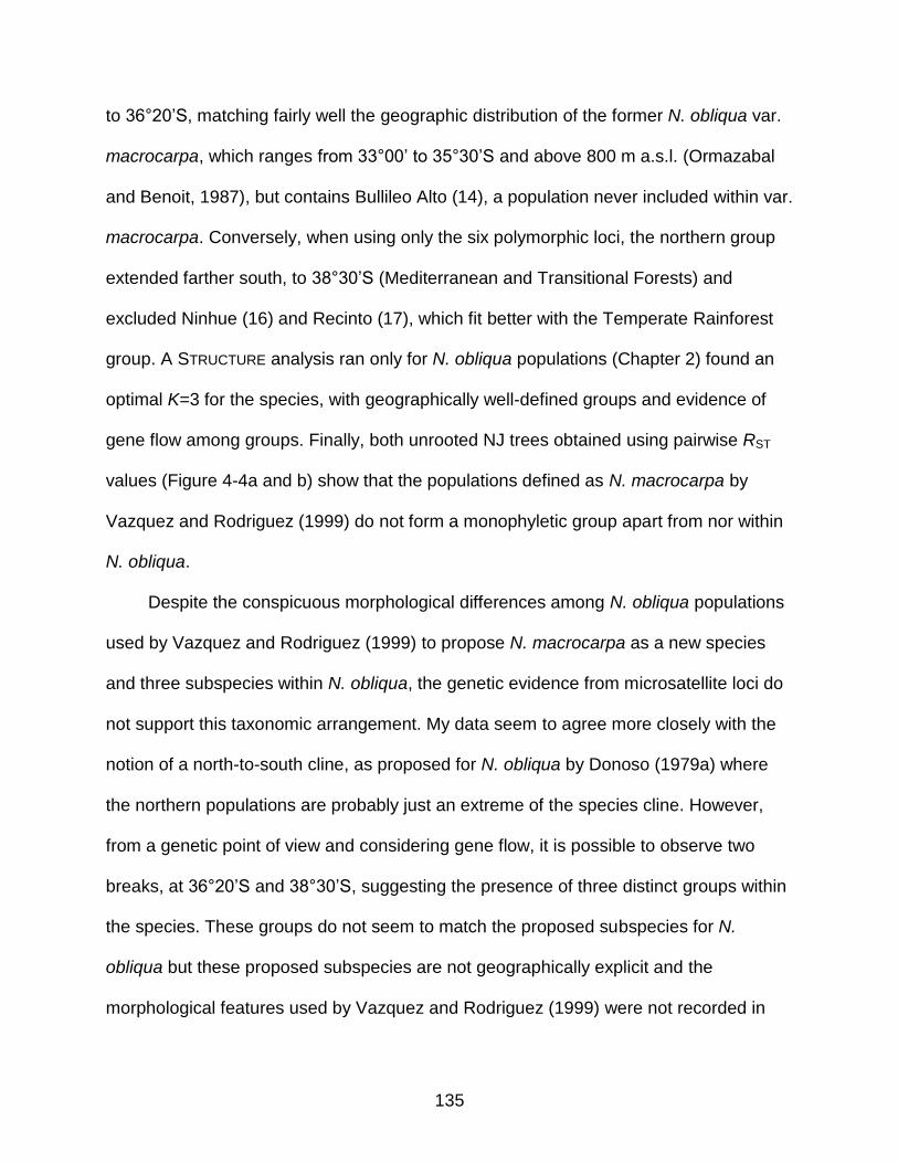
135
to 36°20‟S, matching fairly well the geographic distribution of the former N. obliqua var.
macrocarpa, which ranges from 33°00‟ to 35°30‟S and above 800 m a.s.l. (Ormazabal
and Benoit, 1987), but contains Bullileo Alto (14), a population never included within var.
macrocarpa. Conversely, when using only the six polymorphic loci, the northern group
extended farther south, to 38°30‟S (Mediterranean and Transitional Forests) and
excluded Ninhue (16) and Recinto (17), which fit better with the Temperate Rainforest
group. A STRUCTURE analysis ran only for N. obliqua populations (Chapter 2) found an
optimal K=3 for the species, with geographically well-defined groups and evidence of
gene flow among groups. Finally, both unrooted NJ trees obtained using pairwise RST
values (Figure 4-4a and b) show that the populations defined as N. macrocarpa by
Vazquez and Rodriguez (1999) do not form a monophyletic group apart from nor within
N. obliqua.
Despite the conspicuous morphological differences among N. obliqua populations
used by Vazquez and Rodriguez (1999) to propose N. macrocarpa as a new species
and three subspecies within N. obliqua, the genetic evidence from microsatellite loci do
not support this taxonomic arrangement. My data seem to agree more closely with the
notion of a north-to-south cline, as proposed for N. obliqua by Donoso (1979a) where
the northern populations are probably just an extreme of the species cline. However,
from a genetic point of view and considering gene flow, it is possible to observe two
breaks, at 36°20‟S and 38°30‟S, suggesting the presence of three distinct groups within
the species. These groups do not seem to match the proposed subspecies for N.
obliqua but these proposed subspecies are not geographically explicit and the
morphological features used by Vazquez and Rodriguez (1999) were not recorded in
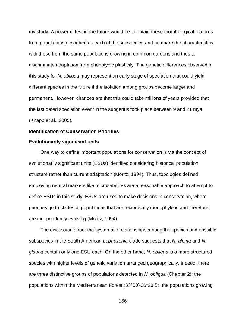
136
my study. A powerful test in the future would be to obtain these morphological features
from populations described as each of the subspecies and compare the characteristics
with those from the same populations growing in common gardens and thus to
discriminate adaptation from phenotypic plasticity. The genetic differences observed in
this study for N. obliqua may represent an early stage of speciation that could yield
different species in the future if the isolation among groups become larger and
permanent. However, chances are that this could take millions of years provided that
the last dated speciation event in the subgenus took place between 9 and 21 mya
(Knapp et al., 2005).
Identification of Conservation Priorities
Evolutionarily significant units
One way to define important populations for conservation is via the concept of
evolutionarily significant units (ESUs) identified considering historical population
structure rather than current adaptation (Moritz, 1994). Thus, topologies defined
employing neutral markers like microsatellites are a reasonable approach to attempt to
define ESUs in this study. ESUs are used to make decisions in conservation, where
priorities go to clades of populations that are reciprocally monophyletic and therefore
are independently evolving (Moritz, 1994).
The discussion about the systematic relationships among the species and possible
subspecies in the South American Lophozonia clade suggests that N. alpina and N.
glauca contain only one ESU each. On the other hand, N. obliqua is a more structured
species with higher levels of genetic variation arranged geographically. Indeed, there
are three distinctive groups of populations detected in N. obliqua (Chapter 2): the
populations within the Mediterranean Forest (33°00‟-36°20‟S), the populations growing
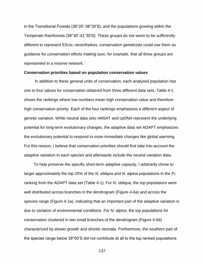
137
in the Transitional Forests (36°20‟-38°30‟S), and the populations growing within the
Temperate Rainforests (38°30‟-41°30‟S). These groups do not seem to be sufficiently
different to represent ESUs; nevertheless, conservation geneticists could use them as
guidance for conservation efforts making sure, for example, that all three groups are
represented in a reserve network.
Conservation priorities based on population conservation values
In addition to these general units of conservation, each analyzed population has
one to four values for conservation obtained from three different data sets. Table 4-1
shows the rankings where low numbers mean high conservation value and therefore
high conservation priority. Each of the four rankings emphasizes a different aspect of
genetic variation. While neutral data sets nMSAT and cpDNA represent the underlying
potential for long-term evolutionary changes, the adaptive data set ADAPT emphasizes
the evolutionary potential to respond to more immediate changes like global warming.
For this reason, I believe that conservation priorities should first take into account the
adaptive variation in each species and afterwards include the neutral variation data.
To help preserve the specific short-term adaptive capacity, I arbitrarily chose to
target approximately the top 25% of the N. obliqua and N. alpina populations in the PT
ranking from the ADAPT data set (Table 4-1). For N. obliqua, the top populations were
well distributed across branches in the dendrogram (Figure 4-6a) and across the
species range (Figure 4-1a), indicating that an important part of the adaptive variation is
due to variation of environmental conditions. For N. alpina, the top populations for
conservation clustered in two small branches of the dendrogram (Figure 4-6b)
characterized by slower growth and shorter stomata. Forthermore, the southern part of
the species range below 39°00‟S did not contribute at all to the top ranked populations
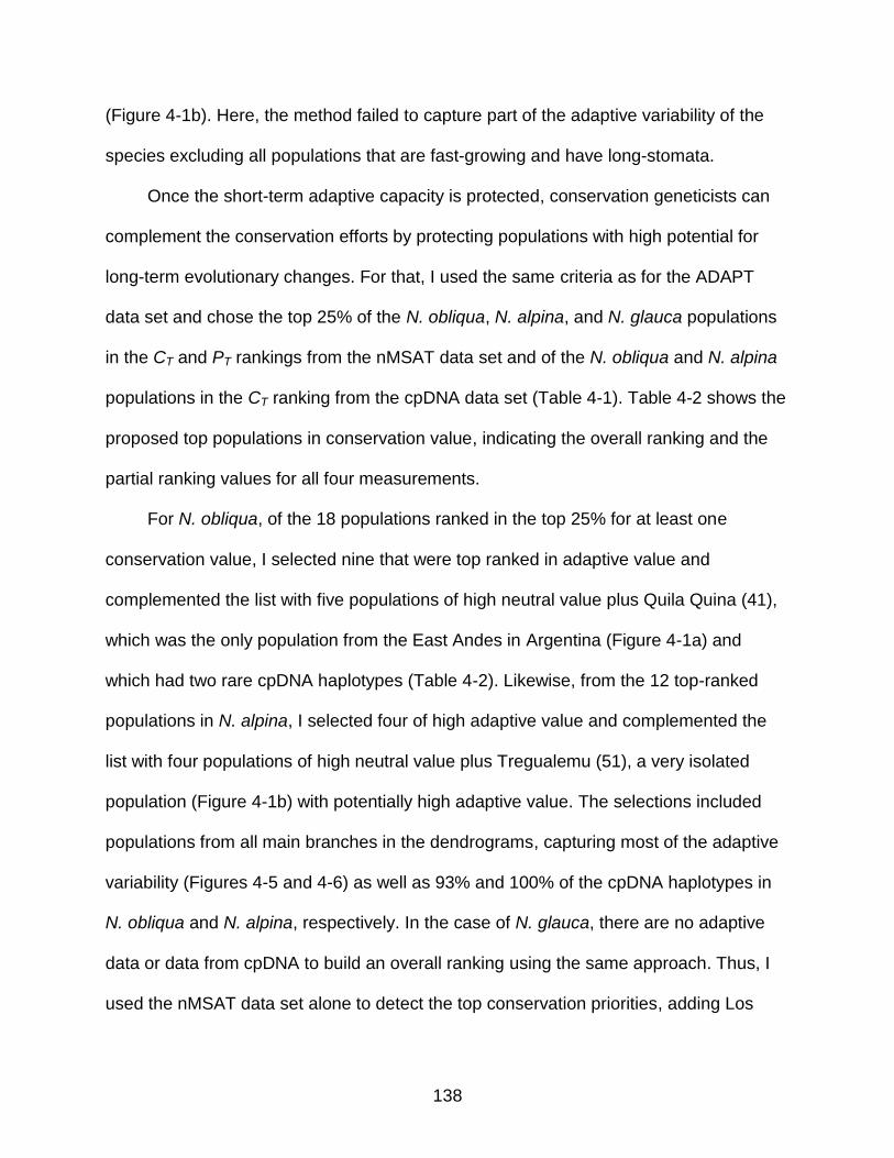
138
(Figure 4-1b). Here, the method failed to capture part of the adaptive variability of the
species excluding all populations that are fast-growing and have long-stomata.
Once the short-term adaptive capacity is protected, conservation geneticists can
complement the conservation efforts by protecting populations with high potential for
long-term evolutionary changes. For that, I used the same criteria as for the ADAPT
data set and chose the top 25% of the N. obliqua, N. alpina, and N. glauca populations
in the CT and PT rankings from the nMSAT data set and of the N. obliqua and N. alpina
populations in the CT ranking from the cpDNA data set (Table 4-1). Table 4-2 shows the
proposed top populations in conservation value, indicating the overall ranking and the
partial ranking values for all four measurements.
For N. obliqua, of the 18 populations ranked in the top 25% for at least one
conservation value, I selected nine that were top ranked in adaptive value and
complemented the list with five populations of high neutral value plus Quila Quina (41),
which was the only population from the East Andes in Argentina (Figure 4-1a) and
which had two rare cpDNA haplotypes (Table 4-2). Likewise, from the 12 top-ranked
populations in N. alpina, I selected four of high adaptive value and complemented the
list with four populations of high neutral value plus Tregualemu (51), a very isolated
population (Figure 4-1b) with potentially high adaptive value. The selections included
populations from all main branches in the dendrograms, capturing most of the adaptive
variability (Figures 4-5 and 4-6) as well as 93% and 100% of the cpDNA haplotypes in
N. obliqua and N. alpina, respectively. In the case of N. glauca, there are no adaptive
data or data from cpDNA to build an overall ranking using the same approach. Thus, I
used the nMSAT data set alone to detect the top conservation priorities, adding Los
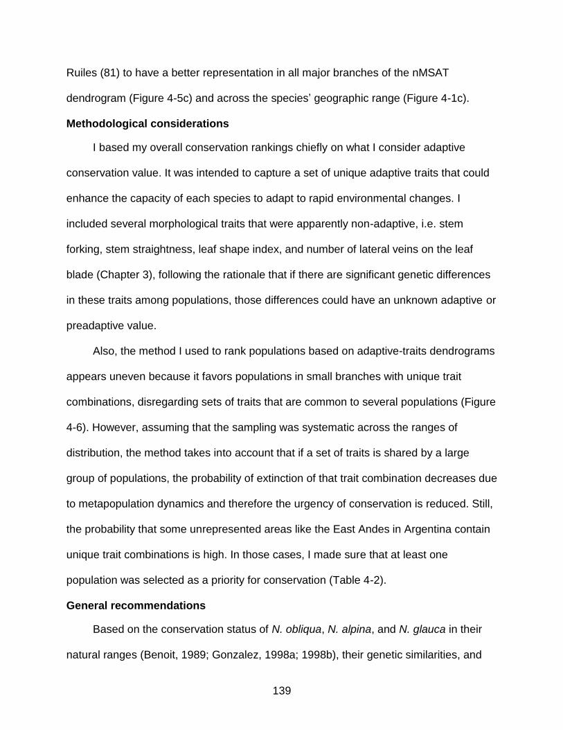
139
Ruiles (81) to have a better representation in all major branches of the nMSAT
dendrogram (Figure 4-5c) and across the species‟ geographic range (Figure 4-1c).
Methodological considerations
I based my overall conservation rankings chiefly on what I consider adaptive
conservation value. It was intended to capture a set of unique adaptive traits that could
enhance the capacity of each species to adapt to rapid environmental changes. I
included several morphological traits that were apparently non-adaptive, i.e. stem
forking, stem straightness, leaf shape index, and number of lateral veins on the leaf
blade (Chapter 3), following the rationale that if there are significant genetic differences
in these traits among populations, those differences could have an unknown adaptive or
preadaptive value.
Also, the method I used to rank populations based on adaptive-traits dendrograms
appears uneven because it favors populations in small branches with unique trait
combinations, disregarding sets of traits that are common to several populations (Figure
4-6). However, assuming that the sampling was systematic across the ranges of
distribution, the method takes into account that if a set of traits is shared by a large
group of populations, the probability of extinction of that trait combination decreases due
to metapopulation dynamics and therefore the urgency of conservation is reduced. Still,
the probability that some unrepresented areas like the East Andes in Argentina contain
unique trait combinations is high. In those cases, I made sure that at least one
population was selected as a priority for conservation (Table 4-2).
General recommendations
Based on the conservation status of N. obliqua, N. alpina, and N. glauca in their
natural ranges (Benoit, 1989; Gonzalez, 1998a; 1998b), their genetic similarities, and
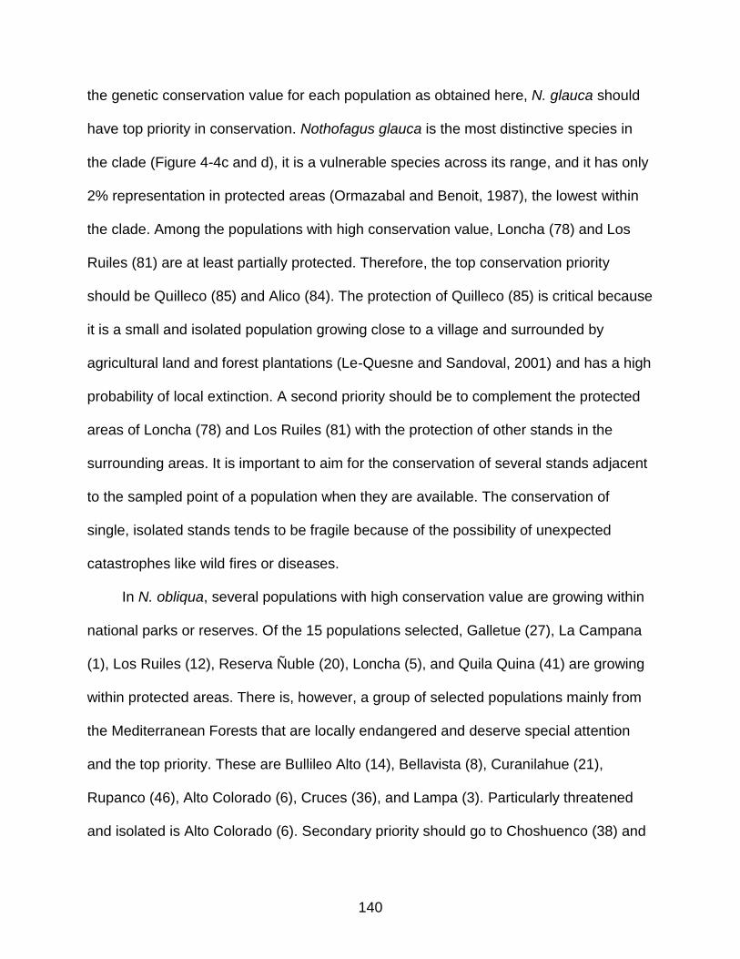
140
the genetic conservation value for each population as obtained here, N. glauca should
have top priority in conservation. Nothofagus glauca is the most distinctive species in
the clade (Figure 4-4c and d), it is a vulnerable species across its range, and it has only
2% representation in protected areas (Ormazabal and Benoit, 1987), the lowest within
the clade. Among the populations with high conservation value, Loncha (78) and Los
Ruiles (81) are at least partially protected. Therefore, the top conservation priority
should be Quilleco (85) and Alico (84). The protection of Quilleco (85) is critical because
it is a small and isolated population growing close to a village and surrounded by
agricultural land and forest plantations (Le-Quesne and Sandoval, 2001) and has a high
probability of local extinction. A second priority should be to complement the protected
areas of Loncha (78) and Los Ruiles (81) with the protection of other stands in the
surrounding areas. It is important to aim for the conservation of several stands adjacent
to the sampled point of a population when they are available. The conservation of
single, isolated stands tends to be fragile because of the possibility of unexpected
catastrophes like wild fires or diseases.
In N. obliqua, several populations with high conservation value are growing within
national parks or reserves. Of the 15 populations selected, Galletue (27), La Campana
(1), Los Ruiles (12), Reserva Ñuble (20), Loncha (5), and Quila Quina (41) are growing
within protected areas. There is, however, a group of selected populations mainly from
the Mediterranean Forests that are locally endangered and deserve special attention
and the top priority. These are Bullileo Alto (14), Bellavista (8), Curanilahue (21),
Rupanco (46), Alto Colorado (6), Cruces (36), and Lampa (3). Particularly threatened
and isolated is Alto Colorado (6). Secondary priority should go to Choshuenco (38) and
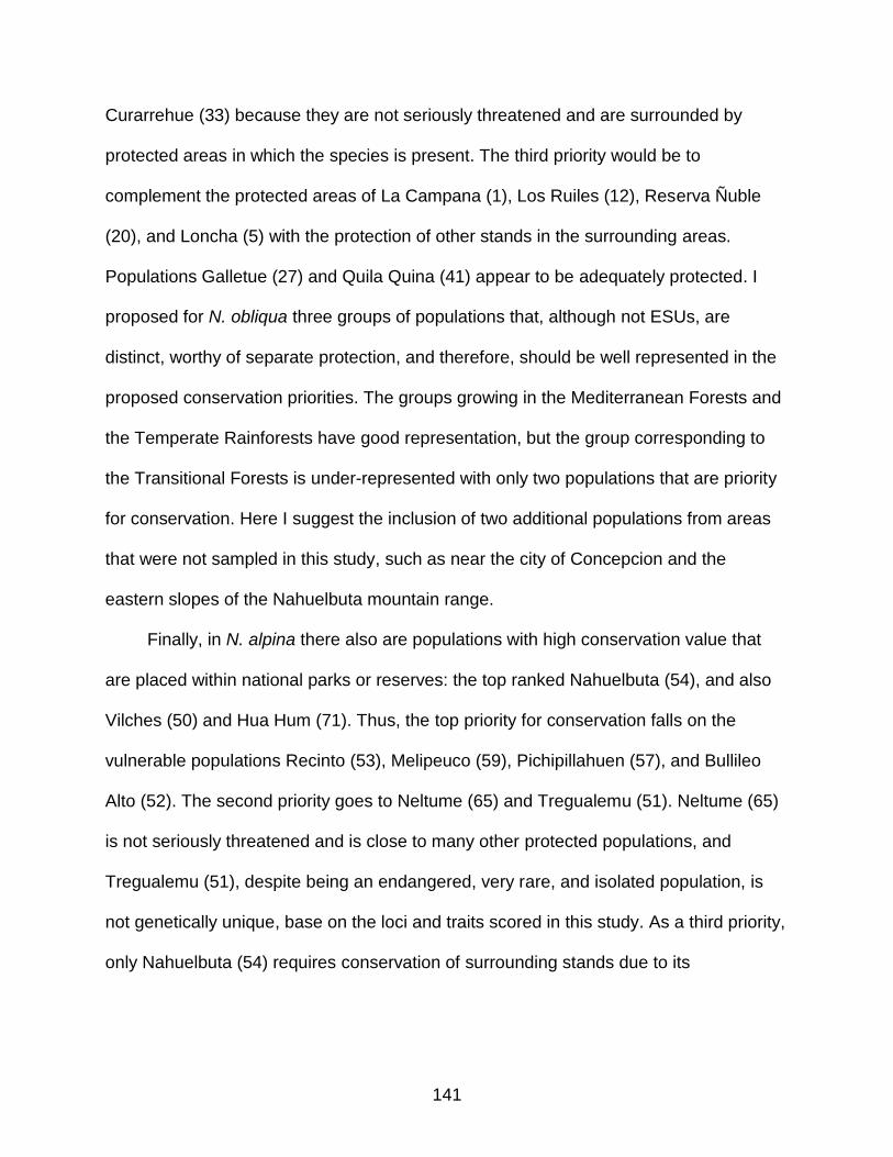
141
Curarrehue (33) because they are not seriously threatened and are surrounded by
protected areas in which the species is present. The third priority would be to
complement the protected areas of La Campana (1), Los Ruiles (12), Reserva Ñuble
(20), and Loncha (5) with the protection of other stands in the surrounding areas.
Populations Galletue (27) and Quila Quina (41) appear to be adequately protected. I
proposed for N. obliqua three groups of populations that, although not ESUs, are
distinct, worthy of separate protection, and therefore, should be well represented in the
proposed conservation priorities. The groups growing in the Mediterranean Forests and
the Temperate Rainforests have good representation, but the group corresponding to
the Transitional Forests is under-represented with only two populations that are priority
for conservation. Here I suggest the inclusion of two additional populations from areas
that were not sampled in this study, such as near the city of Concepcion and the
eastern slopes of the Nahuelbuta mountain range.
Finally, in N. alpina there also are populations with high conservation value that
are placed within national parks or reserves: the top ranked Nahuelbuta (54), and also
Vilches (50) and Hua Hum (71). Thus, the top priority for conservation falls on the
vulnerable populations Recinto (53), Melipeuco (59), Pichipillahuen (57), and Bullileo
Alto (52). The second priority goes to Neltume (65) and Tregualemu (51). Neltume (65)
is not seriously threatened and is close to many other protected populations, and
Tregualemu (51), despite being an endangered, very rare, and isolated population, is
not genetically unique, base on the loci and traits scored in this study. As a third priority,
only Nahuelbuta (54) requires conservation of surrounding stands due to its
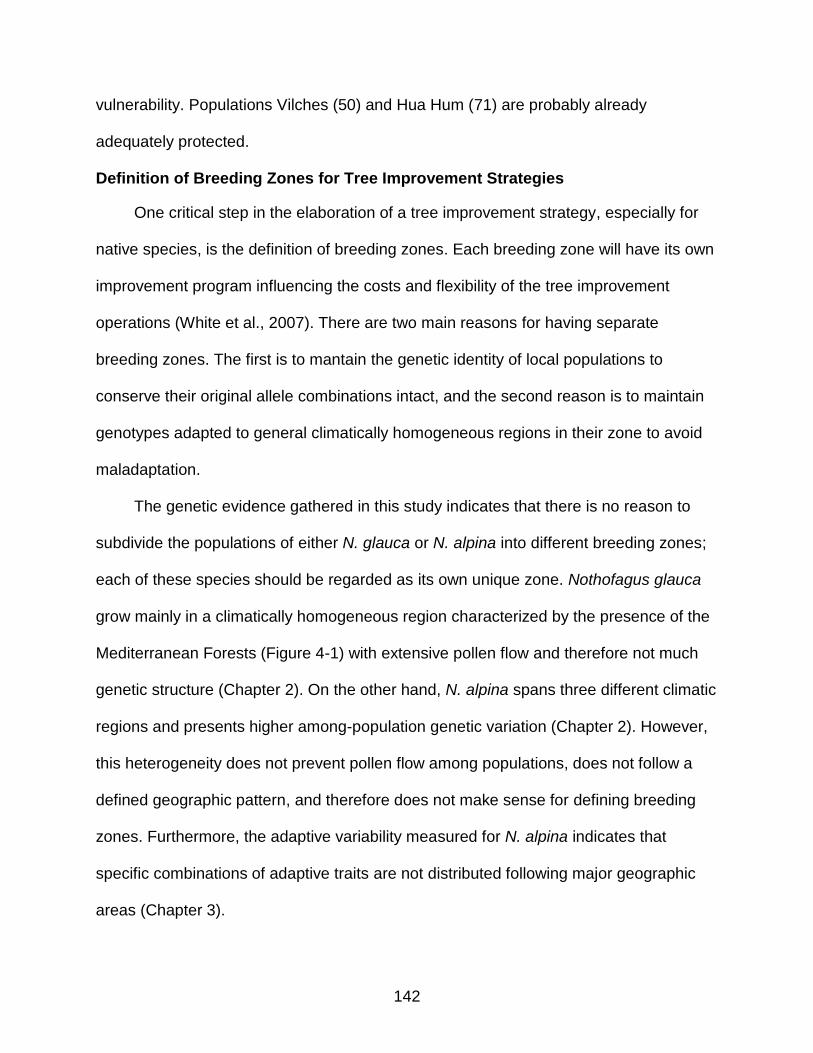
142
vulnerability. Populations Vilches (50) and Hua Hum (71) are probably already
adequately protected.
Definition of Breeding Zones for Tree Improvement Strategies
One critical step in the elaboration of a tree improvement strategy, especially for
native species, is the definition of breeding zones. Each breeding zone will have its own
improvement program influencing the costs and flexibility of the tree improvement
operations (White et al., 2007). There are two main reasons for having separate
breeding zones. The first is to mantain the genetic identity of local populations to
conserve their original allele combinations intact, and the second reason is to maintain
genotypes adapted to general climatically homogeneous regions in their zone to avoid
maladaptation.
The genetic evidence gathered in this study indicates that there is no reason to
subdivide the populations of either N. glauca or N. alpina into different breeding zones;
each of these species should be regarded as its own unique zone. Nothofagus glauca
grow mainly in a climatically homogeneous region characterized by the presence of the
Mediterranean Forests (Figure 4-1) with extensive pollen flow and therefore not much
genetic structure (Chapter 2). On the other hand, N. alpina spans three different climatic
regions and presents higher among-population genetic variation (Chapter 2). However,
this heterogeneity does not prevent pollen flow among populations, does not follow a
defined geographic pattern, and therefore does not make sense for defining breeding
zones. Furthermore, the adaptive variability measured for N. alpina indicates that
specific combinations of adaptive traits are not distributed following major geographic
areas (Chapter 3).
143
The case of N. obliqua is different because the genetic evidence indicates that
there are three groups of populations that could be regarded as different breeding
zones. Like N. alpina, N. obliqua spans three different climatic regions and presents
among-population levels of genetic variation in between those of N. alpina and N.
glauca (Chapter 2). The distinction is that this differentiation shows a geographic pattern
that matches fairly well the north-to-south climatic variation and follows the general
definition of Mediterranean Forests, Transitional Forest, and Temperate Rainforests.
Also, the AMOVA in Chapter 2 reveals that the extensive gene flow among populations
is not the rule when measured among groups, supporting the idea of using three
different breeding zones in a tree improvement strategy.
Nevertheless, defining two breeding zones may be more appropriate for N.
obliqua. Observing the among-group differences in adaptive traits, the Transitional
Forests group always grouped with either the Mediterranean Forests or the Temperate
Rainforests and was never significantly different from both of them at the same time. In
all growth traits and in stomatal length, the Transitional Forests group is similar to the
Temperate Rainforest group, indicating similar overall adaptation to southern climates
(Chapter 3). Thus, my recommendation is to define two breeding zones with separate
tree improvement programs in N. obliqua: breeding zone “North” for the populations
growing within the Mediterranean Forests boundaries (33°00‟-36°20‟S), and breeding
zone “South” for the populations growing southward (36°20‟-41°30‟S).
The current tree improvement strategy developed for N. obliqua and N. alpina
(Ipinza and Gutierrez, 2000) do not propose within-species breeding zones. However,
the priorities stated in the strategy and the implementation of the breeding program for

144
N. obliqua do not include selections outside the Temperate Rainforests and therefore do
not conflict with the zoning stated in my study. The breeding zones definition in N.
obliqua does not coincide with the major macroclimates identified for central Chile
(Fuenzalida, 1965) but coincides well with the boundaries of the regions of provenance
proposed by Vergara (2000). Thus, breeding zone North is comprised of regions of
provenance 1-C, 2-C, and 8-A, while breeding zone South contains all other regions of
provenance.
The translocation of seeds among provenances and among regions of
provenances within each breeding zone should be done with caution. Pollen flow from
translocated trees into a new population should not be a problem because it would be
similar to the extensive pollen flow that seems to occur naturally within each breeding
zone, and therefore the effects on genetic identity should be limited. However, seed
production from the translocated trees will certainly alter the chloroplast composition in
populations of unique haplotypes like those found for N. obliqua (Azpilicueta et al.,
2009) and N. alpina (Marchelli and Gallo, 2006) in certain coastal populations. Gene
flow via seeds in Nothofagus is much slower than pollen flow and in isolated populations
is an extremely rare event. As a result, the effects of translocating plants with a different
haplotype composition will result in a serious long-term threat to genetic identity and
eventually to genetic variability. For this reason, it is important to widen the chloroplast
haplotype characterization in this group to include other isolated populations and more
individuals per population in N. obliqua and N. alpina, and also to include N. glauca.
Once there is information about the chloroplast composition of enough populations, it
will be necessary to limit translocations only to individuals with matching haplotypes.
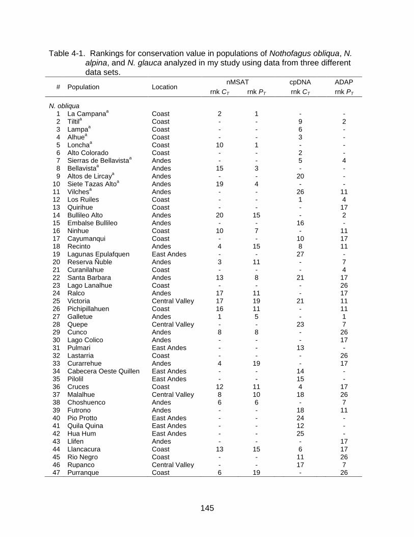
145
Table 4-1. Rankings for conservation value in populations of Nothofagus obliqua, N. alpina, and N. glauca analyzed in my study using data from three different data sets.
# Population Location nMSAT cpDNA ADAP
rnk CT rnk PT rnk CT rnk PT
N. obliqua
1 La Campana
a Coast 2 1 - -
2 Tiltila Coast - - 9 2
3 Lampaa Coast - - 6 -
4 Alhuea Coast - - 3 -
5 Lonchaa Coast 10 1 - -
6 Alto Colorado Coast - - 2 - 7 Sierras de Bellavista
a Andes - - 5 4
8 Bellavistaa Andes 15 3 - -
9 Altos de Lircaya Andes - - 20 -
10 Siete Tazas Altoa Andes 19 4 - -
11 Vilchesa Andes - - 26 11
12 Los Ruiles Coast - - 1 4 13 Quirihue Coast - - - 17 14 Bullileo Alto Andes 20 15 - 2 15 Embalse Bullileo Andes - - 16 - 16 Ninhue Coast 10 7 - 11 17 Cayumanqui Coast - - 10 17 18 Recinto Andes 4 15 8 11 19 Lagunas Epulafquen East Andes - - 27 - 20 Reserva Ñuble Andes 3 11 - 7 21 Curanilahue Coast - - - 4 22 Santa Barbara Andes 13 8 21 17 23 Lago Lanalhue Coast - - - 26 24 Ralco Andes 17 11 - 17 25 Victoria Central Valley 17 19 21 11 26 Pichipillahuen Coast 16 11 - 11 27 Galletue Andes 1 5 - 1 28 Quepe Central Valley - - 23 7 29 Cunco Andes 8 8 - 26 30 Lago Colico Andes - - - 17 31 Pulmari East Andes - - 13 - 32 Lastarria Coast - - - 26 33 Curarrehue Andes 4 19 - 17 34 Cabecera Oeste Quillen East Andes - - 14 - 35 Pilolil East Andes - - 15 - 36 Cruces Coast 12 11 4 17 37 Malalhue Central Valley 8 10 18 26 38 Choshuenco Andes 6 6 - 7 39 Futrono Andes - - 18 11 40 Pio Protto East Andes - - 24 - 41 Quila Quina East Andes - - 12 - 42 Hua Hum East Andes - - 25 - 43 Llifen Andes - - - 17 44 Llancacura Coast 13 15 6 17 45 Rio Negro Coast - - 11 26 46 Rupanco Central Valley - - 17 7 47 Purranque Coast 6 19 - 26
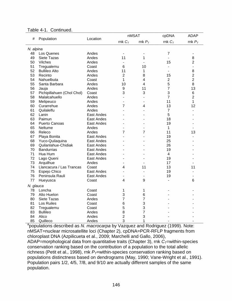
146
Table 4-1. Continued.
# Population Location nMSAT cpDNA
ADAP
rnk CT rnk PT rnk CT
rnk PT
N. alpina
48 Los Quenes Andes - - 7 - 49 Siete Tazas Andes 11 1 - 8 50 Vilches Andes - - 15 2 51 Tregualemu Coast 6 10 - - 52 Bullileo Alto Andes 11 1 - 8 53 Recinto Andes 2 8 15 2 54 Nahuelbuta Coast 1 4 2 2 55 Santa Barbara Andes 10 4 5 8 56 Jauja Andes 9 11 7 13 57 Pichipillahuen (Chol Chol) Coast 3 3 3 6 58 Malalcahuello Andes - - 7 2 59 Melipeuco Andes - - 11 1 60 Curarrehue Andes 7 4 13 12 61 Quilalelfu Andes - - 7 - 62 Lanin East Andes - - 5 - 63 Paimun East Andes - - 18 - 64 Puerto Canoas East Andes - - 19 - 65 Neltume Andes - - 1 - 66 Releco Andes 7 7 11 13 67 Playa Bonita East Andes - - 19 - 68 Yuco-Quilaquina East Andes - - 25 - 69 Quilanlahue-Chidiak East Andes - - 26 - 70 Bandurrias East Andes - - 19 - 71 Hua Hum East Andes - - 4 - 72 Lago Queni East Andes - - 19 - 73 Arquilhue Andes - - 17 - 74 Llancacura / Las Trancas Coast 4 11 13 11 75 Espejo Chico East Andes - - 19 - 76 Peninsula Rauli East Andes - - 19 - 77 Hueyusca Coast 4 9 - 6
N. glauca
78 Loncha Coast 1 1 - - 79 Alto Huelon Coast 3 6 - - 80 Siete Tazas Andes 7 7 - - 81 Los Ruiles Coast 6 3 - - 82 Tregualemu Coast 5 3 - - 83 Bullileo Andes 8 7 - - 84 Alico Andes 2 3 - - 85 Quilleco Andes 3 1 - -
apopulations described as N. macrocarpa by Vazquez and Rodriguez (1999). Note: nMSAT=nuclear microsatellite loci (Chapter 2), cpDNA=PCR-RFLP fragments from chloroplast DNA (Azpilicueta et al., 2009; Marchelli and Gallo, 2006), ADAP=morphological data from quantitative traits (Chapter 3), rnk CT=within-species conservation ranking based on the contribution of a population to the total allelic richness (Petit et al., 1998), rnk PT=within-species conservation ranking based on populations distinctness based on dendrograms (May, 1990; Vane-Wright et al., 1991). Population pairs 1/2, 4/5, 7/8, and 9/10 are actually different samples of the same population.
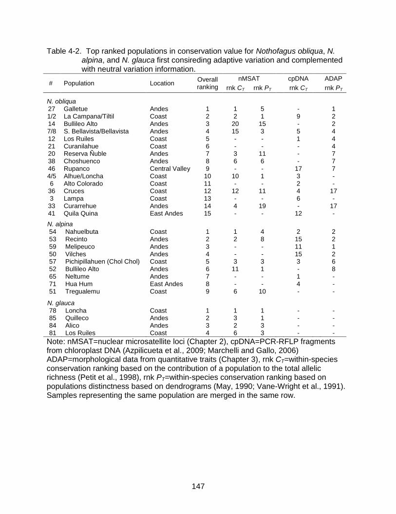
147
Table 4-2. Top ranked populations in conservation value for Nothofagus obliqua, N. alpina, and N. glauca first consireding adaptive variation and complemented with neutral variation information.
# Population Location Overall ranking
nMSAT cpDNA ADAP
rnk CT rnk PT rnk CT rnk PT
N. obliqua
27 Galletue Andes 1 1 5 - 1 1/2 La Campana/Tiltil Coast 2 2 1 9 2 14 Bullileo Alto Andes 3 20 15 - 2 7/8 S. Bellavista/Bellavista Andes 4 15 3 5 4 12 Los Ruiles Coast 5 - - 1 4 21 Curanilahue Coast 6 - - - 4 20 Reserva Ñuble Andes 7 3 11 - 7 38 Choshuenco Andes 8 6 6 - 7 46 Rupanco Central Valley 9 - - 17 7 4/5 Alhue/Loncha Coast 10 10 1 3 - 6 Alto Colorado Coast 11 - - 2 -
36 Cruces Coast 12 12 11 4 17 3 Lampa Coast 13 - - 6 -
33 Curarrehue Andes 14 4 19 - 17 41 Quila Quina East Andes 15 - - 12 -
N. alpina
54 Nahuelbuta Coast 1 1 4 2 2 53 Recinto Andes 2 2 8 15 2 59 Melipeuco Andes 3 - - 11 1 50 Vilches Andes 4 - - 15 2 57 Pichipillahuen (Chol Chol) Coast 5 3 3 3 6 52 Bullileo Alto Andes 6 11 1 - 8 65 Neltume Andes 7 - - 1 - 71 Hua Hum East Andes 8 - - 4 - 51 Tregualemu Coast 9 6 10 - -
N. glauca
78 Loncha Coast 1 1 1 - - 85 Quilleco Andes 2 3 1 - - 84 Alico Andes 3 2 3 - - 81 Los Ruiles Coast 4 6 3 - -
Note: nMSAT=nuclear microsatellite loci (Chapter 2), cpDNA=PCR-RFLP fragments from chloroplast DNA (Azpilicueta et al., 2009; Marchelli and Gallo, 2006) ADAP=morphological data from quantitative traits (Chapter 3), rnk CT=within-species conservation ranking based on the contribution of a population to the total allelic richness (Petit et al., 1998), rnk PT=within-species conservation ranking based on populations distinctness based on dendrograms (May, 1990; Vane-Wright et al., 1991). Samples representing the same population are merged in the same row.
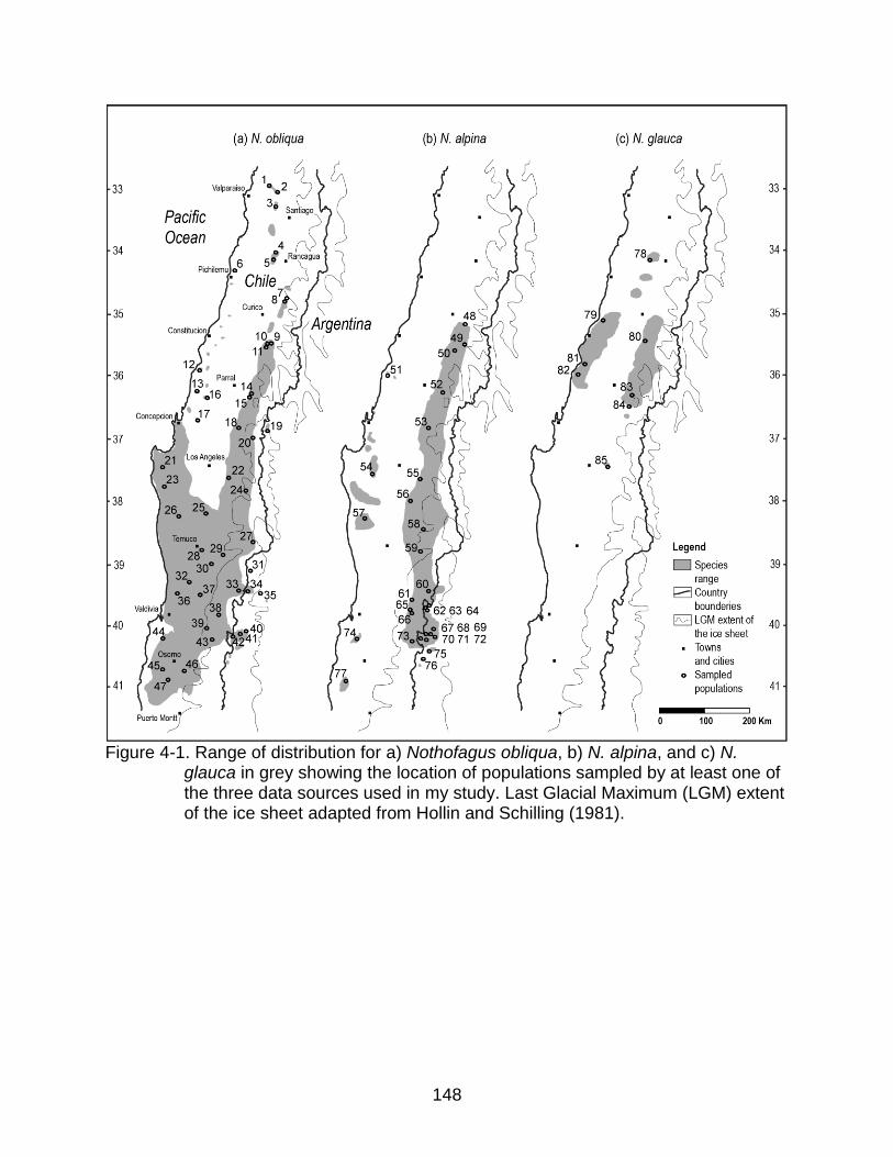
148
Figure 4-1. Range of distribution for a) Nothofagus obliqua, b) N. alpina, and c) N.
glauca in grey showing the location of populations sampled by at least one of the three data sources used in my study. Last Glacial Maximum (LGM) extent of the ice sheet adapted from Hollin and Schilling (1981).
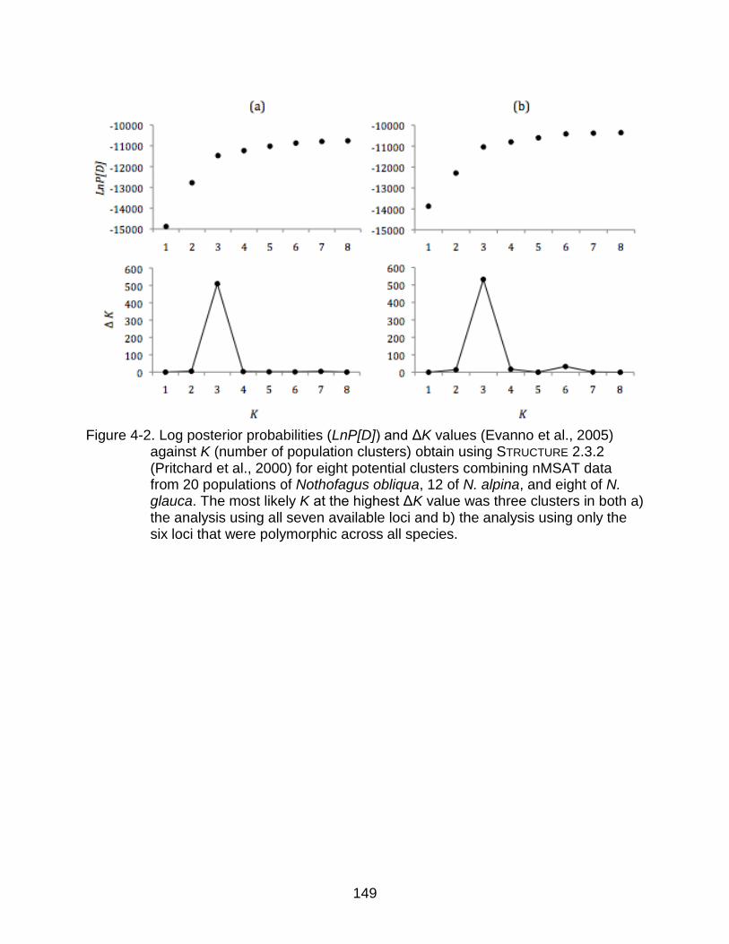
149
Figure 4-2. Log posterior probabilities (LnP[D]) and ΔK values (Evanno et al., 2005)
against K (number of population clusters) obtain using STRUCTURE 2.3.2 (Pritchard et al., 2000) for eight potential clusters combining nMSAT data from 20 populations of Nothofagus obliqua, 12 of N. alpina, and eight of N. glauca. The most likely K at the highest ΔK value was three clusters in both a) the analysis using all seven available loci and b) the analysis using only the six loci that were polymorphic across all species.
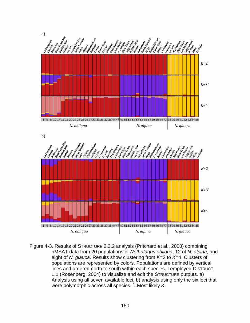
150
Figure 4-3. Results of STRUCTURE 2.3.2 analysis (Pritchard et al., 2000) combining nMSAT data from 20 populations of Nothofagus obliqua, 12 of N. alpina, and eight of N. glauca. Results show clustering from K=2 to K=4. Clusters of populations are represented by colors. Populations are defined by vertical lines and ordered north to south within each species. I employed DISTRUCT 1.1 (Rosenberg, 2004) to visualize and edit the STRUCTURE outputs. a) Analysis using all seven available loci, b) analysis using only the six loci that were polymorphic across all species. *=Most likely K.
N. obliqua N. alpina N. glauca
b)
K=2
K=4
K=3*
. 1 5 8 10 14 16 18 20 22 24 25 26 27 29 33 36 37 38 44 47 .
49 51 52 53 54 55 56 57 60 66 74 77 .
. 78 79 80 81 82 83 84 85
. 1 5 8 10 14 16 18 20 22 24 25 26 27 29 33 36 37 38 44 47 …
49 51 52 53 54 55 56 57 60 66 74 77 .
. 78 79 80 81 82 83 84 85
N. obliqua N. alpina N. glauca
K=2
K=4
K=3*
a)
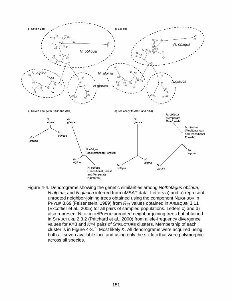
151
Figure 4-4. Dendrograms showing the genetic similarities among Nothofagus obliqua, N.alpina, and N.glauca inferred from nMSAT data. Letters a) and b) represent unrooted neighbor-joining trees obtained using the component NEIGHBOR in PHYLIP 3.69 (Felsenstein, 1989) from RST values obtained in ARLEQUIN 3.11 (Excoffier et al., 2005) for all pairs of sampled populations. Letters c) and d) also represent NEIGHBOR/PHYLIP unrooted neighbor-joining trees but obtained in STRUCTURE 2.3.2 (Pritchard et al., 2000) from allele-frequency divergence values for K=3 and K=4 pairs of STRUCTURE clusters. Membership of each cluster is in Figure 4-3. *=Most likely K. All dendrograms were acquired using both all seven available loci, and using only the six loci that were polymorphic across all species.
N. obliqua
N. alpina
N.glauca
N. obliqua
N. alpina
N.glauca
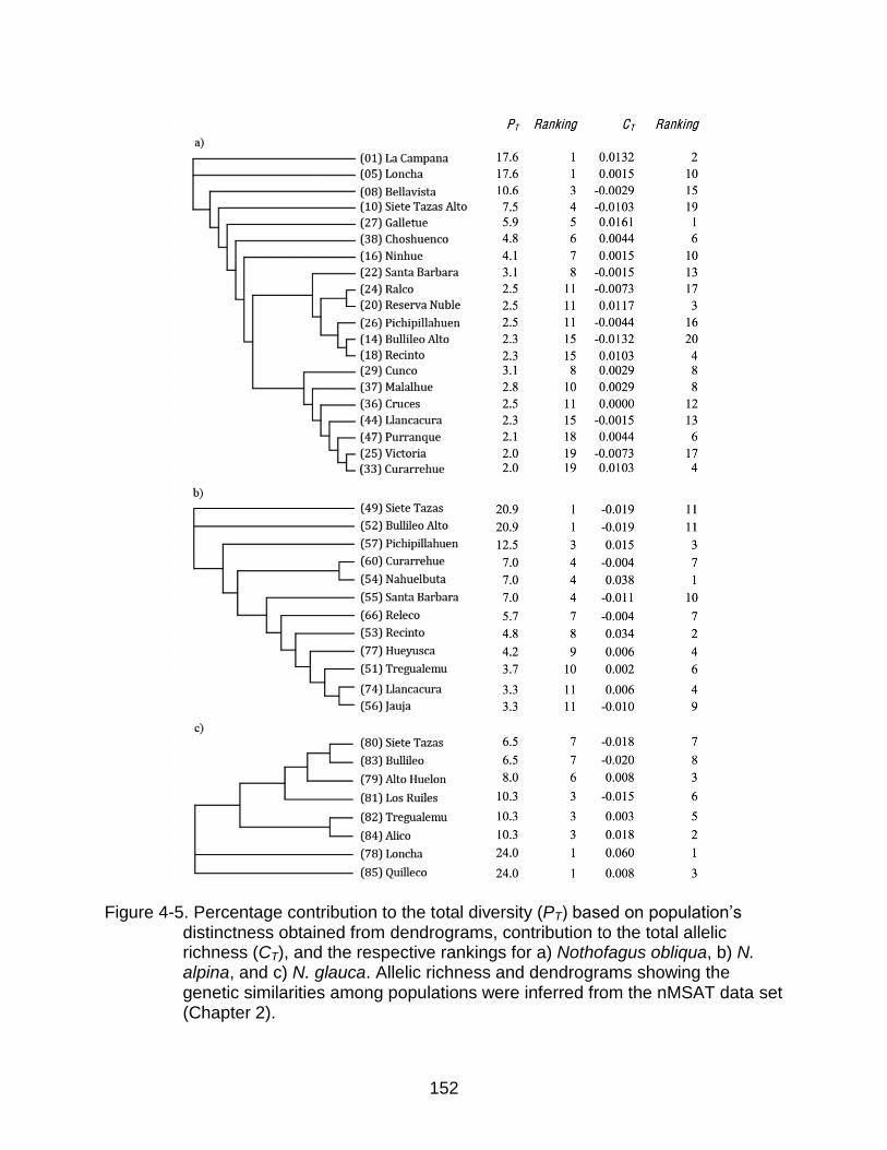
152
Figure 4-5. Percentage contribution to the total diversity (PT) based on population‟s
distinctness obtained from dendrograms, contribution to the total allelic richness (CT), and the respective rankings for a) Nothofagus obliqua, b) N. alpina, and c) N. glauca. Allelic richness and dendrograms showing the genetic similarities among populations were inferred from the nMSAT data set (Chapter 2).
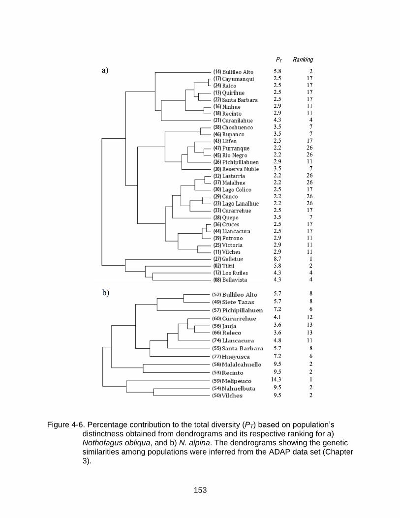
153
Figure 4-6. Percentage contribution to the total diversity (PT) based on population‟s distinctness obtained from dendrograms and its respective ranking for a) Nothofagus obliqua, and b) N. alpina. The dendrograms showing the genetic similarities among populations were inferred from the ADAP data set (Chapter 3).
154
CHAPTER 5 CONCLUSIONS
This study highlights the relatively high levels of neutral genetic variation of the
South American species of Nothofagus subgenus Lophozonia that are in concert with
values of other tree species of similar biology. The genetic structure obtained by neutral
markers was relatively low due to extensive gene flow. However, for growth traits, there
was more structure with moderate values in Nothofagus alpina and high values in N.
obliqua revealing that natural selection is playing an important role in creating adaptive
variation at least in the latter species, which also has a wider ecological range than N.
alpina.
For adaptive traits in general, N. obliqua also has higher levels of individual
heritability, higher coefficients for provenance genetic gains, and more significant
associations of traits with geographic and environmental patterns of variation than N.
alpina. This indicates that N. obliqua may have a better chance to adapt to future
climatic changes through natural selection, and breeders would obtain larger genetic
gains by selecting the correct provenances and best individuals in this species relative
to N. alpina. In N. obliqua, the association of growth, stem straightness, leaf shape, and
stomatal density values with geographic and environmental variation indicates genetic
adaptation to different temperatures and precipitations including the tendency of trees
growing faster when they are from provenances that have similar environmental
conditions than the place where they are planted.
The patterns of neutral genetic variation among and within species obtained in my
study also support: 1) the multiple refugia hypothesis for N. obliqua and N. alpina,
suggesting several centers of genetic diversity across their areas of distribution, 2) a
155
topology within the clade, base on overall genetic similarity, that places N. obliqua and
N. alpina together in a branch and N. glauca as their sister species, 3) the lack of
sufficient genetic structure in N. obliqua to support the placement of its northern
populations in a separate species (i.e. N. macrocarpa) or designations of subspecies
within the remaining populations, and 4) the occurrence of ancient and current
hybridization as a contributor to the intraspecific genetic diversity within the subgenus
and as a major source of variability and differentiation for the northern populations of N.
obliqua.
Finally, combining neutral and adaptive genetic variation in this study allowed me
to propose conservation priorities among and within species and to define breeding
zones within species useful for tree improvement strategies. According to my combined
analysis and also based on the general conservation status of the three species in their
natural ranges, it appears that at the species level N. glauca should have the top priority
for conservation, and then as a second priority, N. obliqua and N. alpina. The choice of
priorities within species and among populations should always go to populations with
outstanding uniqueness in their adaptive characteristics. This list of populations should
then be complemented with other populations with unique alleles and genotypes
obtained from neutral markers. Within these selected populations the top priority is
unprotected, small, isolated populations. The second priority is populations insufficiently
protected, larger in size, or with higher connectivity. In this study I proposed to give high
conservation priority to four, fifteen, and seven areas for N. glauca, N. obliqua, and N.
alpina, respectively.
156
Regarding the definition of breeding zones, my integrated analysis indicates that
there is no reason to subdivide the populations of N. glauca or N. alpina into different
breeding zones; each of these species should be regarded as its own unique zone. For
N. obliqua the genetic evidence using neutral markers indicates that there are three
groups of populations that could be regarded as different breeding zones. Nevertheless,
observing the among-group differences in adaptive traits suggests that defining two
breeding zones may be more appropriate for this species: breeding zone “North” for the
populations growing within the Mediterranean Forests boundaries (33°00‟-36°20‟S), and
breeding zone “South” for the populations growing southward (36°20‟-41°30‟S).
As a final recommendation, the translocation of seeds among populations within
each breeding zone should be done with caution. While pollen flow from trees
translocated into a new population should not be a problem because extensive pollen
flow occurs naturally within breeding zones, seed production from the translocated trees
will certainly alter the chloroplast composition in populations of unique haplotypes
because immigration from seed dispersal is an extremely rare event in isolated
populations. Therefore, translocations may results in the loss of genetic identity and
variability in the long term. For this reason, after a more complete chloroplast haplotype
characterization, it would be desirable to limit translocations only to individuals with
matching haplotypes.
157
LIST OF REFERENCES
Allnutt, T.R., Newton, A.C., Lara, A., Premoli, A.C., Armesto, J.J., Vergara, R., Gardner, M., 1999. Genetic variation in Fitzroya cupressoides (alerce), a threatened South American conifer. Mol. Ecol. 8, 975–987.
Amigo, J., Ramírez, C., 1998. A bioclimatic classification of Chile: woodland communities in the temperate zone. Plant Ecol. 136, 9–26.
Armesto, J.J., Leon-Lobos, P., Arroyo, M.K., 1995. Los bosques templados del sur de Chile y Argentina: Una isla biogeografica. In: Armesto, J.J., Villagran, C., Arroyo, M.K. (Eds.), Ecologia de los bosques natives de Chile. Ed. Universitaria, Santiago, Chile, pp. 23–28.
Azpilicueta, M.M., Caron, H., Gallo, L.A., 2004. SSR markers for analyzing South American Nothofagus species. Silvae Genet. 53, 240–243.
Azpilicueta, M.M., Marchelli, P., Gallo, L.A. 2009. The effects of Quaternary glaciations in Patagonia as evidenced by chloroplast DNA phylogeography of Southern beech Nothofagus obliqua. Tree Genet. Genomes 5, 561–571.
Bekessy, S.A., Allnutt, T.R., Premoli, A.C., Lara, A., Ennos, R.A., Burgman, M.A., Cortes, M., Newton, A.C., 2002. Genetic variation in the vulnerable and endemic Monkey Puzzle tree, detected using RAPDs. Heredity 88, 243–249.
Benoit, I.L. (Ed.), 1989. Red List of Chilean Terrestrial Flora (Part One). CONAF, Santiago, Chile.
Bruschi, P., Vendramin, G.G., Bussotti, F., Grossoni, P., 2003. Morphological and molecular diversity among Italian populations of Quercus petraea (Fagaceae). Ann. Bot. 91, 707–716.
Buiteveld, J., Vendramin, G.G., Leonardi, S., Kamer, K., Geburek, T., 2007. Genetic diversity and differentiation in European beech (Fagus sylvatica L.) stands varying in management history. For. Ecol. Manage. 247, 98–106.
Carrasco, B., Eaton, L., 2002. Natural history and genetic structure of raulí (Nothofagus nervosa (Phil.) Dim. et Mil.). For. Genet. 9, 275–284.
Carrasco, B., Garnier, M., Eaton, L., Guevara, R., Carú, M., 2009. Proximal causes of genetic variation between and within populations of raulí (Nothofagus nervosa). Cien. Inv. Agr. 36, 229–238.
Chultz, F.A., 2003. Evaluacion del comportamiento geografico en parametros seminales y de crecimiento inicial de las plantas, en procedencias de Nothofagus dombeyi (Mirb.) Oerst. B.S. Thesis. Universidad Austral de Chile, Valdivia, Chile.
158
Clausen, J., Keck, D.D., Hiesey, W.M., 1940. Experimental Studies on the Nature of Species. I.Effect of Varied Environments on Western North American Plants. Publication #520. Carnegie Institution of Washington. Washington, DC, US.
Cornelius, J., 1994. Heritabilities and additive genetic coefficients of variation in forest trees. Can. J. For. Res. 24, 372–379.
Craft, K.J., Ashley, M.V., 2007. Landscape genetic structure of bur oak (Quercus macrocarpa) savannas in Illinois. For. Ecol. Manage. 239, 13–20.
Demesure, B., Comps, B., Petit, J., 1996. Chloroplast DNA phylogeography of the common beech (Fagus sylvatica L.) in Europe. Evolution 50, 2515–2520.
Dewoody, J., Nason, J.D., Hipkins, V.D., 2006. Mitigating scoring errors in microsatellite data from wild populations. Mol. Ecol. Notes 6, 951–957.
Di Castri, F., Hajek, E., 1976. Bioclimatología de Chile. Vicerrectoría Académica, U. Católica de Chile, Santiago, Chile.
Donoso, C., 1979a. Genecological differentiation in Nothofagus obliqua (Mirb.) Oerst. in Chile. For. Ecol. Manage. 2, 53–66.
Donoso, C., 1979b. Nothofagus leonii Espinosa, a natural hybrid between Nothofagus obliqua (Mirb.) Orest. and Nothofagus glauca (Phil.) Krasser. New Zeal. J. Bot. 17, 353–360.
Donoso, C., 1982. Resena ecologica de los bosques mediterraneos de Chile. Bosque 4, 117–146.
Donoso, C., 1987. Variacion natural en especies de Nothofagus en Chile. Bosque 8, 85–95.
Donoso, C., 1993. Bosques templados de Chile y Argentina. Variacion, estructura y dinamica, first ed. Editorial Universitaria, Santiago, Chile.
Donoso, C., Morales, J., Romero, M., 1990. Natural hybridization between Nothofagus obliqua (Mirb.) Oerst. and N. alpina (Poepp. and Endl.) Oerst. in forests of southern Chile. Rev. Chil. Hist. Nat. 63, 49–60.
Donoso, P., Donoso, C., Sandoval, V., 1993. Proposición de zonas de crecimiento de renovales de roble (Nothofagus obliqua) y raulí (Nothofagus alpina) en su rango de distribución natural. Bosque 14, 37–55.
Doyle, J.J., Doyle, J.L., 1987. A rapid isolation procedure for small quantities of fresh tissue. Phytochem. Bull. 19, 11–15.
159
Evanno, G., Regnaut, S., Goudet, J., 2005. Detecting the number of clusters of individuals using the software Structure: a simulation study. Mol. Ecol. 14, 2611–2620.
Excoffier, L., Estoup, A., Cornuet, J-M., 2005. Bayesian analysis of an admixture model with mutations and arbitrarily linked markers. Genetics 169, 1727–1738.
Excoffier, L., Laval, G., Schneider, S., 2005. Arlequin ver. 3.0: An integrated software package for population genetics data analysis. Evol. Bioinform. Online 1, 47–50.
Faith, D.P., 1992. Conservation evaluation and phylogenetic diversity. Biol. Conserv. 61, 1–10.
Faith, D.P., 1994. Genetic diversity and taxonomic priorities for conservation. Biol. Conserv. 68, 69–74.
Falush, D., Stephens, M., Pritchard, J.K., 2003. Inference of population structure using multilocus genotype data: linked loci and correlated allele frequencies. Genetics 164, 1567–1587.
Felsenstein, J., 1989. PHYLIP - Phylogeny Inference Package (Version 3.2). Cladistics 5, 164–166.
Frantz, A.C., Cellina, S., Krier, A., Schley, L., Burke, T., 2009. Using spatial Bayesian methods to determine the genetic structure of a continuously distributed population: clusters or isolation by distance? J. Appl. Ecol. 46, 493–505.
Fuenzalida, H., 1965. Clima. In: Geografia economica de Chile. Texto refundido. Corporacion de Fomento de la Produccion (CORFO), Santiago, Chile, pp. 99–152.
Gallo, L.A., Marchelli, P., Breitembucher, A., 1997. Morphological and allozymic evidence of natural hybridization between two southern beeches (Nothofagus spp.) and its relation to heterozygosity and height growth. For. Genet. 4, 15–23.
Gilmour, A.R., Gogel, B.J., Cullis, B.R., Thompson, R., 2006. ASReml User Guide Release 2.0. VSN International Ltd, Hemel Hempstead.
Gitzendanner, M.A., Soltis, P.S., 2000. Patterns of genetic variation in rare and widespread plant congeners. Am. J. Bot. 87, 783–792.
Goldstein, D.B., Ruiz Linares, A., Cavalli-Sforza, L.L., Feldman, M.W., 1995. An evaluation of genetic distances for use with microsatellite loci. Genetics 139, 463–471.
Gonzalez, M., 1998a. Nothofagus alpina. In: IUCN 2010. IUCN Red List of Threatened Species. Version 2010.4. <www.iucnredlist.org>. Downloaded on 20 May 2011.
160
Gonzalez, M., 1998b. Nothofagus glauca. In: IUCN 2010. IUCN Red List of Threatened Species. Version 2010.4. <www.iucnredlist.org>. Downloaded on 20 May 2011.
Gutiérrez, B., Ipinza, R., 2000. Evaluación de parámetros genéticos en Nothofagus. In: Ipinza, R., Gutiérrez, B., Emhart, V. (Eds.), Domesticación y Mejora Genética de Roble y Raulí. Universidad Austral de Chile / Instituto Forestal, Valdivia, Chile, pp. 371–390.
Haase, P., 1992. Isozyme variability and biogeography of Nothofagus truncata (Fagaceae). New Zeal. J. Bot. 30, 315–328.
Haase, P., 1993. Genetic variation, gene flow, and the 'founder effect' in pioneer populations of Nothofagus menziesii (Fagaceae), South Island, New Zealand. J. Biogeogr. 20, 79–85.
Hamrick, J.L., 1982. Plant population genetics and evolution. Am. J. Bot. 69, 1685–1693.
Hamrick, J.L., 2004. Response of forest trees to global environmental changes. For. Ecol. Manage. 197, 323–335.
Hamrick, J.L., Godt, M.J.W., 1996. Effects of life history traits on genetic diversity in plant species. Philos. T. R. Soc. B 351, 1291–1298.
Heusser, C.J., 1990. Ice-age vegetation and climate of subtropical Chile. Palaeogeogr., Palaeoclimatol., Palaeoecol. 80, 107–127.
Hewitt, G., 2000. The genetic legacy of the Quaternary ice ages. Nature 405, 907–913.
Hiraoka, K., Tomaru, N., 2009. Population genetic structure of Fagus japonica revealed by nuclear microsatellite markers. Int. J. Plant Sci. 170, 748–758.
Hodge, G.R., Dvorak, W.S., 2004. The CAMCORE international provenance-progeny trials of Gmelina arborea: genetic parameters and potential gain. New For. 28, 147–166.
Hollin, J.T., Schilling, D.H., 1981. Late Wisconsin-Weichselian mountain glaciers and small ice caps. In: Denton, G.H., Hughes, T.J. (Eds.), The Last Great Ice Sheets. Wiley, New York, USA, pp. 179–206.
Hovenden, M.J., 2001. The influence of temperature and genotype on growth and stomatal morphology of southern beech, Nothofagus cunninghamii (Nothofagaceae). Aust. J. Bot. 49, 427–434.
Hovenden, M.J., Vander Schoor, J.K., 2003. Nature vs nurture in the leaf morphology of Southern beech, Nothofagus cunninghamii (Nothofagaceae). New Phytol. 161, 585–594.
161
Hovenden, M.J., Vander Schoor, J.K., 2006. The response of leaf morphology to irradiance depends on altitude of origin in Nothofagus cunninghamii. New Phytol. 169, 291–297.
Ipinza, R., Espejo, J., 2000. Biologia reproductiva en Nothofagus. In: Ipinza, R., Gutierrez, B., Emhart, V. (Eds.), Domesticacion y mejora genetica de rauli y roble. Universidad Austral de Chile / Instituto Forestal, Valdivia, Chile, pp. 75–93.
Ipinza R., Gutierrez, B., 2000. Estrategia de mejora genetica para N. alpina and N. obliqua. In: Ipinza, R., Gutierrez, B., Emhart, V. (Eds.), Domesticacion y mejora genetica de rauli y roble. Universidad Austral de Chile / Instituto Forestal, Valdivia, Chile, pp. 403–417.
Ipinza, R., Gutiérrez, B., Medina, A., 2000. Variación genética del peso y forma de la semilla y crecimiento inicial de procedencias naturales de N. alpina y N. obliqua en Chile. In: Ipinza, R., Gutierrez, B., Emhart, V. (Eds.), Domesticacion y mejora genetica de rauli y roble. Universidad Austral de Chile / Instituto Forestal, Valdivia, Chile, pp. 323–347.
Jones, R.C., Vaillancourt, R.E., Jordan, G.J., 2004. Microsatellites for use in Nothofagus cunninghamii (Nothofagaceae) and related species. Mol. Ecol. Notes 4, 14–16.
Kalinowski, S.T., 2004. Counting alleles with rarefaction: Private alleles and hierarchical sampling designs. Conserv. Genet. 5, 539–543.
Kalinowski, S.T., 2005. HP-RARE 1.0: a computer program for performing rarefaction on measures of allelic richness. Mol. Ecol. Notes 5, 187–189.
Knapp, M., Stockler, K., Havell, D., Delsuc, F., Sebastiani, F., Lockhart, P.J., 2005. Relaxed molecular clock provides evidence for long-distance dispersal of Nothofagus (southern beech). Plos Biol. 3, 38–43.
Landry, P.A., Koskinen, M.T., Primmer, C.R., 2002. Deriving evolutionary relationships
among populations using microsatellites and ( μ)2: all loci are equal, but some are more equal than others ... Genetics 161, 1339–1347.
Ledgard, N.J., Norton, D.A., 1988. Shoot growth in 2-3 year old Nothofagus seedlings. New Zeal. J. Ecol. 11, 105–108.
Lee, Y.J., Hwang, S.Y., Ho, K.C., Lin, T.P., 2006. Source populations of Quercus glauca in the last glacial age in Taiwan revealed by nuclear microsatellite markers. J. Hered. 97, 261–269.
Le-Quesne, C., Sandoval, L., 2001. New southern limit for Nothofagus glauca (Phil.) Krasser. Gayana, 58, 139–142.
162
Li, P., Beaulieu, J., Corriveau, A., Bousquet, J., 1993. Genetic variation in juvenile growth and phenology of white spruce provenance-progeny test. Silvae Genet. 42, 52–60.
Luebert, F., Pliscoff, P., 2006. Sinopsis bioclimática y vegetacional de Chile. Editorial Universitaria, Santiago, Chile.
Magri, D., Vendramin, G.G., Comps, B., Dupanloup, I., Geburek, T., Gomory, D., Latatowa, M., Litt, T., Paule, L., Roure, J.M., Tantau, I., van der Knaap, W.O., Petit, R.J., de Beaulieu, J-L., 2006. A new scenario for the Quaternary history of European beech populations: palaeobotanical evidence and genetic consequences. New Phytol. 171, 199–221.
Manos, P.S., 1997. Systematics of Nothofagus (Nothofagaceae) based on rDNA spacer sequences (ITS): Taxonomic congruence with morphology and plastid sequences. Am. J. Bot. 84, 1137–1155.
Moritz, C., 1994. Defining „Evolutionary Significant Units‟ for conservation. Trends Ecol. Evol. 9, 373–375.
Marchelli, P., Caron, H., Azpilicueta, M.M., Gallo, L.A., 2008. Primer note: A new set of highly polymorphic nuclear microsatellite markers for Nothofagus nervosa and related South American species. Silvae Genet. 57, 82–85.
Marchelli, P., Gallo, L., Scholz, F., Ziegenhagen, B., 1998. Chloroplast DNA markers reveal a geographical divide across Argentinean southern beech Nothofagus nervosa (Phil.) Dim. et Mil. distribution area. Theor. Appl. Genet. 97, 642–646.
Marchelli, P., Gallo, L.A., 2001. Genetic diversity and differentiation in a southern beech subjected to introgressive hybridization. Heredity 87, 284–293.
Marchelli, P., Gallo, L.A., 2004. The combined role of glaciation and hybridization in shaping the distribution of genetic variation in a Patagonian southern beech. J. Biogeogr. 31, 451–460.
Marchelli, P., Gallo, L.A., 2006. Multiple ice-age refugia in a southern beech of South America as evidenced by chloroplast DNA markers. Conserv. Genet. 7, 591–603.
Markgraf, V., Romero, E.J., Villagran, C., 1996. History and Paleoecology of South American Nothofagus forests. In: Veblen, T.T., Hill, R.S., Read, J. (Eds.), The ecology and biogeography of Nothofagus forests. Yale University Press, New Haven & London, pp. 354–386.
Marsico TD, Hellmann JJ, Romero-Severson J (2009) Patterns of seed dispersal and pollen flow in Quercus garryana (Fagaceae) following post-glacial climatic changes. J. Biogeogr. 36, 929–941.
163
Matheson, A.C., 1989. Statistical methods and problems in testing large numbers of genotypes across sites. In: Gibson, G.L., Griffin, A.R., Matheson, A.C. (Eds.), Breeding Tropical Trees: Population Structure and Genetic Improvement Strategies in Clonal and Seedling Forestry. Proceedings IUFRO meeting, 28 November–3 December 1988, Pattaya, Thailand. Oxford Forestry Institute, Oxford, UK, pp. 93-105.
Mathiasen, P., Premoli, A.C., 2010. Out in the cold: genetic variation of Nothofagus pumilio (Nothofagaceae) provides evidence for latitudinally distinct evolutionary histories in austral South America. Mol. Ecol. 19, 371–385.
May, R. M., 1990. Taxonomy as destiny. Nature 347, 129–130.
McGarigal, K., Cushman, S., Stafford, S., 2000. Multivariate statistics for wildlife and ecology research. Springer-Verlag New York, Inc.
McKay, J.K., Latta, R.G., 2002. Adaptive population divergence: markers, QTL and traits. Trends Ecol. Evol. 17, 285–291.
Medina, A.M., 2001. Evaluacion del comportamiento genetico y geografico en parametros seminales y de crecimiento inicial de las plantas, en procedencias de Nothofagus alpina (Poep. et Endl.) Oerst.). B.S. Thesis. Universidad Austral de Chile, Valdivia, Chile.
Millerón, M., Gallo, L., Marchelli, P., 2008. The effect of volcanism on postglacial migration and seed dispersal. A case study in southern South America. Tree Genet. Genomes 4, 435–443.
Moreno, P.I., Lowell, T.V., Jacobson, G.L., Denton, G.H., 1999. Abrupt vegetation and climate changes during the last glacial maximum and last termination in the Chilean Lake District: A case study from Canal de la Puntilla (41°S). Geogr. Ann. A 81, 285–311.
Muir, G., Lowe, A.J., Fleming, C.C., Vogl, C., 2004. High nuclear genetic diversity, high levels of outcrossing and low differentiation among remnant populations of Quercus petraea at the margin of its range in Ireland. Ann. Bot. 93, 691–697.
Nei, M., 1973. Analysis of gene diversity in subdivided populations. P. Natl. Acad. Sci. USA 70, 3321–3323.
Nunez-Avila, M.C., Armesto, J.J., 2006. Relict islands of the temperate rainforest tree Aextoxicon punctatum (Aextoxicaceae) in semi-arid Chile: genetic diversity and biogeographic history. Aust. J. Bot. 54, 733–743.
Ogden, J., 1989. On the coenospecies concept and tree migrations during the oscillations of the Pleistocene climate. J. Roy. Soc. New Zeal. 19, 249–262.
164
Ormazabal, C., Benoit, I., 1987. El estado de conservacion del genero Nothofagus en Chile. Bosque 8, 109–120.
Page, R.D.M., 1996. TreeView: An application to display phylogenetic trees on personal computers. Comput. Appl. Biosci. 12, 357–358.
Pakkad, G., Ueno, S., Yoshimaru, H., 2008. Genetic diversity and differentiation of Quercus semiserrata Roxb. in northern Thailand revealed by nuclear and chloroplast microsatellite markers. For. Ecol. Manage. 255, 1067–1077.
Pastorino, M.J., Marchelli, P., Milleron, M., Soliani, C., Gallo, L.A., 2009. The effect of different glaciation patterns over the current genetic structure of the southern beech Nothofagus antarctica. Genetica 136, 79–88.
Petit, R.J., Aguinagalde, I., de Beaulieu, J.L., Bittkau, C., Brewer, S., Cheddadi, R., Ennos, R., Fineschi, S., Grivet, D., Lascoux, M., Mohanty, A., Müller-Starck, G., Demesure-Musch, B., Palmé, A., Martín, J.P., Rendell, S., Vendramin, G.G., 2003. Glacial refugia: hotspots but not melting pots of genetic diversity. Science 300, 1563–1565.
Petit, R.J., El Mousadik, A., Pons, O., 1998. Identifying populations for conservation on the basis of genetic markers. Conserv. Biol. 12, 844–855.
Pineda, G., 2000. Variabilidad aloenzimatica de N. alpina en Chile. In: Ipinza, R., Gutierrez, B., Emhart, V. (Eds.), Domesticacion y mejora genetica de rauli y roble. Universidad Austral de Chile / Instituto Forestal, Valdivia, Chile, pp. 95–119.
Premoli, A.C., 1997. Genetic variation in a geographically restricted and two widespread species of South American Nothofagus. J. Biogeogr. 24, 883–892.
Premoli, A.C., Vergara, R., Souto, C.P., Lara, A., Newton, A.C., 2003. Lowland valleys shelter the ancient conifer Fitzroya cupressoides in the Central Depression of southern Chile. J. Roy. Soc. New Zeal. 33, 623–631.
Premoli, A.C., Brewer, C.A., 2007. Environmental v. genetically driven variation in ecophysiological traits of Nothofagus pumilio from contrasting elevations. Aust. J. Bot. 55, 585–591.
Premoli, A.C., Raffaele, E., Mathiasen, P., 2007. Morphological and phenological differences in Nothofagus pumilio from contrasting elevations: Evidence from a common garden. Austral Ecol. 32, 515–523.
Pritchard, J.K., Stephens, M., Donnelly, P., 2000. Inference of population structure using multilocus genotype data. Genetics 155, 945–959.
Puntieri, J.G., Grosfeld, J.E., Stecconi, M., Brion, C., Azpilicueta, M.M., Gallo, L., 2006. Desarrollo temprano del roble (Nothofagus obliqua): un analisis arquitectural de procedencias de Argentina. Bosque 27, 44–51.
165
Reed, D.H., Frankham, R., 2001. How closely correlated are molecular and quantitative measures of genetic variation? A meta-analysis. Evolution 55, 1095–1103.
Rempel, R.S., Carr, A.P. 2003. Patch Analyst 3.1 Extension for ARCGIS® 9.1. Available
from http://flash.lakeheadu.ca/~rrempel/patch/index.html. Accessed March 2008.
Rice, W.R., 1989. Analyzing tables of statistical tests. Evolution 43, 223–225.
Riveros, M., Parades, M.A., Rosas, M.T., Cardenas, E., Armesto, J., Arroyo, M.K., Palma, B., 1995. Reproductive biology in species of the genus Nothofagus. Environ. Exp. Bot. 35, 519–524.
Rodriguez, J., Medina, A. 2000. Viverización de procedencias de N. alpina y N. obliqua en contenedores. In: Ipinza, R., Gutiérrez, B., Emhart, V. (Eds.), Domesticación y Mejora Genética de Roble y Raulí. Universidad Austral de Chile / Instituto Forestal, Valdivia, Chile, pp. 307-322.
Romero, H., 1985. Geografía de los climas. Tomo XI. Colección de geografía de Chile. Editorial IGM, Santiago, Chile.
Rosenberg, N.A., 2004. Distruct: a program for the graphical display of population structure. Mol. Ecol. Notes 4, 137–138.
Rousset, F., 1996. Equilibrium values of measures of population subdivision for stepwise mutation processes. Genetics 142, 1357–1362.
Rousset, F., 2008. Genepop'007: a complete reimplementation of the Genepop software for Windows and Linux. Mol. Ecol. Res. 8, 103–106.
Santelices, R., Navarro, R.M., Drake, F., 2009. Caracterizacion del material forestal de reproduccion de cinco procedencias de Nothofagus alessandrii Espinosa, una especie en peligro de extincion. Interciencia 34, 113–120.
SAS, 2008. SAS/STAT , software release 9.2, SAS Institute Inc. Cary, NC.
Schwarz, G.E., 1978. Estimating the dimension of a model. Ann. Stat. 6, 461–464.
Sebbenn, A.M., Pontinha, A.A.S., Giannotti, E., Kageyama, P.Y., 2003. Genetic variation in provenance-progeny test of Araucaria angustifolia (bert.) O. Ktze. in Sao Paulo, Brazil. Silvae Genet. 52, 181–184.
Selkoe, K.A., Toonen, R.J., 2006. Microsatellites for ecologists: a practical guide to using and evaluating microsatellite markers. Ecol. Lett. 9, 615–629.
Sepulveda, C.A., Stoll, A., 2003. Nothofagus alpina (Poepp. et Endl.) Oerst. (Fagaceae) in the coastal area of the Maule Region, central Chile. Gayana Bot. 60, 132–133.
166
Sierra-Lucero, V., McKeand, S.E., Huber, D.A., Rockwood, D.L., White, T.L., 2002. Performance differences and genetic parameters for four coastal provenances of loblolly pine in the Southeastern United States. For. Sci. 48, 732–742.
Slatkin, M., 1995. A measure of population subdivision based on microsatellite allele frequencies. Genetics 139, 457–462.
Soltis, D.E., Gitzendanner, M.A., Strenge, D.D., Soltis, P.S., 1997. Chloroplast DNA intraspecific phylogeography of plants from the Pacific Northwest of North America. Plant Syst. Evol. 206, 353–373.
Soltis, D.E., Morris, A.B., McLachlan, J.S., Manos, P.S., Soltis, P.S., 2006. Comparative phylogeography of unglaciated eastern North America. Mol. Ecol. 15, 4261–4293.
Squillace, A. E., 1974. Average genetic correlations among offspring from open-pollinated forest trees. Silvae Genet. 23, 149–156.
Steubing, L., Godoy, R., Alberdi, M., 2002. Metodos de ecologia vegetal. Editorial Universitaria, Santiago, Chile.
Sun, O.J., Sweet, G.B., 1996. Comparison of frost tolerance of Nothofagus solandri var. cliffortioides (Hook. f.) Poole and Nothofagus menziesii (Hook. f.) Oerst. New Zeal. J. Bot. 34, 273–278.
Taberlet, P., Fumagalli, L., Wust-Saucy, A-G., Cosson, J-F., 1998. Comparative phylogeography and postglacial colonization routes in Europe. Mol. Ecol. 7, 453–464.
Taylor, K.J., Lowe, A.J., Hunter, R.J., Ridgway, T., Gresshoff, P.M., Rossetto, M., 2005. Genetic diversity and regional identity in the Australian remnant Nothofagus moorei. Aust. J. Bot. 53, 437–444.
Tchatchoua, D. T., Aravanopoulos, F. A. 2010a. Evaluation of selected European chestnut (Castanea sativa) provenances - I: Inter-provenance genetic variation. Acta Hort. 866, 203–213.
Tchatchoua, D. T., Aravanopoulos, F. A. 2010b. Evaluation of selected European chestnut (Castanea sativa) provenances - II: Intra-provenance family variation. Acta Hort. 866, 215–224.
Thiele, R., Moreno, H., Elgueta, S., Lahsen, A., Rebolledo, S., Petit-Breuilh, M., 1998. Evolucion geologico-geomorfologica cuaternaria del tramo superior del valle del rio Laja. Rev. Geol. Chile 25, 229–253.
Torres-Diaz, C., Ruiz, E., Gonzalez, F., Fuentes, G., Cavieres, L.A., 2007. Genetic diversity in Nothofagus alessandrii (Fagaceae), an endangered endemic tree species of the coastal maulino forest of central Chile. Ann. Bot. 100, 75–82.
167
van Oosterhout, C., Hutchinson, W.F., Wills, D.P.M., Shipley, P., 2004. Micro-Checker: software for identifying and correcting genotyping errors in microsatellite data. Mol. Ecol. Notes 4, 535–538.
van Tienderen, P.H., de Haan, A.A., van der Linden, C.G., Vosman B., 2002. Biodiversity assessment using markers for ecologically important traits. Trends Ecol. Evol. 17, 577–582.
Vane-Wright, R.I., Humphries, C.J., Williams, P.H., 1991. What to protect? Systematics and the agony of choice. Biol. Conserv. 55, 235–254.
Vazquez, F.M., Rodriguez, R.A., 1999. A new subspecies and two new combinations of Nothofagus Blume (Nothofagaceae) from Chile. Bot. J. Linn. Soc., 129, 75–83.
Veblen, T., Schlegel, F., 1982. Resena ecologica de los bosques del sur de Chile. Bosque 4, 73–115.
Vergara, R., 2000. Regiones de procedencia de N. alpina y N. obliqua. In: Ipinza, R., Gutierrez, B., Emhart, V. (Eds.), Domesticacion y mejora genetica de rauli y roble. Universidad Austral de Chile / Instituto Forestal, Valdivia, Chile, pp. 121–132.
Vergara, R., Bohle, K., 2000. Estado actual del recurso forestal de N. alpina y N. obliqua. In: : Ipinza, R., Gutierrez, B., Emhart, V. (Eds.), Domesticacion y mejora genetica de rauli y roble. Universidad Austral de Chile / Instituto Forestal, Valdivia, Chile, pp. 40–52.
Villagran, C., 1991. Historia de los bosques templados del sur de Chile durante el Tardiglacial y Postglacial. Rev. Chil. Hist. Nat. 64, 447–460.
Villagran, C., 2001. A model for the history of vegetation of the Coastal Range of central-southern Chile: Darwin's glacial hypothesis. Rev. Chil. Hist. Nat. 74, 793–803.
Villagran, C., Moreno, P., Villa, R., 1995. Antecedentes palinologicos acerca de la historia cuaternaria de los bosques chilenos. In: Armesto, J.J., Villagran, C., Arroyo, M.K. (Eds.), Ecologia de los bosques nativos de Chile. Editorial Universitaria, Santiago, Chile, pp. 51–70.
White, T.L., Adams, W.T., Neale, D.B., 2007. Forest genetics. Wallingford, Oxfordshire, UK, CABI Pub.
Wightman, K.E., Ward, S.E., Haggar, J.P., Santiago, B.R., Cornelius, J.P., 2008. Performance and genetic variation of big-leaf mahogany (Swietenia macrophylla King) in provenance and progeny trials in the Yucatan Peninsula of Mexico. For. Ecol. Manage. 255, 346–355.
Wilcox, M.D., Ledgard, N.J., 1983. Provenance variation in the New Zealand species of Nothofagus. New Zeal. J. Ecol. 6, 19–31.
168
Worth, J.R.P., Jordan, G.J., McKinnon, G.E., Vaillancourt, R.E., 2009. The major Australian cool temperate rainforest tree Nothofagus cunninghamii withstood Pleistocene glacial aridity within multiple regions: evidence from the chloroplast. New Phytol. 182, 519–532.
Wright, S., 1931. Evolution in Mendelian populations. Genetics 16, 97–159.
Wright, S., 1943. Isolation by distance. Genetics 28, 114–138.
Wright, S., 1965. The interpretation of population structure by F-statistics with special regard to systems of mating. Evolution 19, 395–420.
Xie, C.Y., 2008. Ten-year results from red alder (Alnus rubra Bong.) provenance-progeny testing and their implications for genetic improvement. New For. 36, 273–284.
Zobel, B., Talbert, J., 1984. Applied Forest Tree Improvement. John Wiley and Sons, Inc., NY, USA.
169
BIOGRAPHICAL SKETCH
Rodrigo Vergara was born in Santiago, Chile in 1969, and was raised in Chillan
about 400 km south of Santiago, where he went to school in Colegio Padre A. Hurtado.
After high school he moved south to Valdivia roughly 450 km south of Chillan, to study
Forest Engineering at Universidad Austral de Chile where he graduated on 1995 with
his undergraduate thesis “Grafting methods in raulí (Nothofagus alpina (Poepp. et.
Endl.) Oerst)”. Right after he graduated, Rodrigo started his career as an Instructor in
Forest Genetics in the Department of Silviculture at Universidad Austral de Chile where
he participated on several projects related to tree breeding and conservation genetics.
In 2000 he returned to school to pursue his Masters of Science in Forest Genetics in the
School of Forest Resources and Conservation at the University of Florida where he
graduated in 2003 with his thesis, “Estimation of realized genetic gains and validation of
predicted breeding values using field trials with large rectangular plots of slash pine
(Pinus elliottii var. elliottii)”. To complete his PhD, Rodrigo moved to the Department of
Botany, currently Department of Biology, under the advisement of Dr. Pamela S. Soltis
and graduated in 2011.