REVIEW ARTICLE

Neuroevolution: from architectures to learning

Dario Floreano Æ Peter Durr Æ Claudio Mattiussi

Received: 5 October 2007 / Accepted: 17 October 2007 / Published online: 10 January 2008

� Springer-Verlag 2008

Abstract Artificial neural networks (ANNs) are applied

to many real-world problems, ranging from pattern clas-

sification to robot control. In order to design a neural

network for a particular task, the choice of an architecture

(including the choice of a neuron model), and the choice of

a learning algorithm have to be addressed. Evolutionary

search methods can provide an automatic solution to these

problems. New insights in both neuroscience and evolu-

tionary biology have led to the development of increasingly

powerful neuroevolution techniques over the last decade.

This paper gives an overview of the most prominent

methods for evolving ANNs with a special focus on recent

advances in the synthesis of learning architectures.

Keywords Neural networks � Evolution � Learning

1 Introduction

Over the last 50 years, researchers from a variety of fields

have used models of biological neural networks not only to

better understand the workings of biological nervous sys-

tems, but also to devise powerful tools for engineering

applications.

Artificial neural networks (ANNs) are computational

models implemented in software or specialized hardware

devices that attempt to capture the behavioral and adaptive

features of biological nervous systems. They are typically

composed of several interconnected processing units, or

‘neurons’ (see Fig. 1) which can have a number of inputs

and outputs. In mathematical terms, an ANN can be seen as

a directed graph where each node implements a neuron

model. In the simplest case, the neuron model is just a

weighted sum of the incoming signals transformed by a

(typically nonlinear) static transfer function. More sophis-

ticated neuron models involve discrete-time or continuous-

time dynamics (see Sect. 3). The connection strengths

associated with the edges of the graph connecting two

neurons are referred to as synaptic weights, the neurons

with connections to the external environment are often

called input or output neurons, respectively. The number

and type of neurons and the set of possible interconnections

between them define the architecture or topology of the

neural network.

In order to solve computational or engineering problems

with neural networks, learning algorithms are used to find

suitable network parameters. Evolutionary algorithms

provide an interesting alternative, or complement, to the

commonly used learning algorithms, such as back-propa-

gation [68, 69]. Evolutionary algorithms are a class of

population-based, stochastic search methods inspired by

the principles of Darwinian evolution. Instead of using a

conventional learning algorithm, the characteristics of

neural networks can be encoded in artificial genomes and

evolved according to a performance criterion. The advan-

tages of using an evolutionary algorithm instead of another

learning method are that several defining features of the

neural network can be genetically encoded and co-evolved

at the same time and that the definition of a performance

D. Floreano � P. Durr (&) � C. Mattiussi

Ecole Polytechnique Federale de Lausanne Laboratory

of Intelligent Systems, Station 11, 1015 Lausanne, Switzerland

e-mail: peter.duerr@epfl.ch

URL: http://lis.epfl.ch

D. Floreano

e-mail: dario.floreano@epfl.ch

C. Mattiussi

e-mail: claudio.mattiussi@epfl.ch

123

Evol. Intel. (2008) 1:47–62

DOI 10.1007/s12065-007-0002-4

criterion is more flexible than the definition of an energy or

error function. Furthermore, evolution can be coupled with

a learning algorithm such as Hebbian learning [32], or even

used to generate new learning algorithms. In the following

we give an overview of the recent methods for evolving

ANNs. Since to our knowledge there is no systematic

large-scale comparison of the different approaches we

focus on the most-widely used canonical methods and

some of the most promising recent developments. We first

review approaches that evolve the network architecture and

its parameters. Then we give a short overview of the most

prominent dynamic neuron models used in neuroevolution

experiments. We then move on to describe different

methods for combining evolution and learning, including

the evolutionary synthesis of novel learning algorithms.

Finally we point to recent work aiming at evolving archi-

tectures capable of controlling learning events.

2 Evolution of neural architectures

The evolutionary synthesis of a neural network leads to

several design choices. Besides the choice of an appro-

priate fitness function and the setting of appropriate

evolutionary parameters, e.g., population size or mutation

rates, the key problem is the choice of suitable genetic

representations that recombination and mutation operators

can manipulate to discover high-fitness networks with high

probability. We can classify current representations into

three classes: direct, developmental and implicit. Although

all three representations can be used to evolve both the

network topology and its parameters, developmental and

implicit representations offer more flexibility for evolving

neural topologies whereas direct representations have been

used mainly for evolving the parameter values of fixed-size

networks.

2.1 Direct Representations

In a direct representation, there is a one-to-one mapping

between the parameter values of the neural network and the

genes that compose the genetic string. In the simplest case,

synaptic weights and other parameters (e.g., bias weights or

time-constants) of a fixed network topology are directly

encoded in the genotype either as a string of real values or

as a string of characters, which are then interpreted as real-

values with a given precision. This can be done by inter-

preting the string of characters as a binary or Gray-coded

number. However, this strategy requires the knowledge of

the suitable intervals and precision of the encoded param-

eters. In order to make the mapping more adaptive,

Schraudolph and Belew [73] suggested a dynamic encod-

ing, where the bits allocated for each weight are used to

encode the most significant part of the binary representa-

tion until the population has converged to a satisfactory

solution. At that point, those same bits are used to encode

the less significant part of the binary representation in order

to narrow the search and refine the performance of the

evolutionary network. Another possibility is to use a self-

adaptive encoding such as the Center of Mass Encoding

suggested by Mattiussi et al. [45], where the characters of

the string are interpreted as a system of particles whose

center of mass determines the encoded value. The advan-

tage of this method is that it automatically adapts the

granularity of the representation to the requirements of the

task.

Recent benchmark experiments with Evolution Strate-

gies [62], which use a floating-point representation of the

synaptic weights, have reported excellent performance with

direct encoding of a small, fixed architecture [38]. In these

experiments, Igel used an evolution strategy called

covariance matrix adaptation (CMA-ES). CMA-ES is an

evolutionary algorithm that generates new candidate solu-

tions by sampling from a multivariate normal distribution

over the search space and changes this mutation distribu-

tion by adapting its covariance matrix [30].

In a classic study, Montana and Davis [51] compared the

performance of synaptic weight evolution with a discrete

direct representation with that of the back-propagation

Fig. 1 A generic neural network architecture. It consists of Inputunits and Output units which are connected to the external environ-

ment and Hidden units which connect to other neurons but are not

directly connected to the environment

48 Evol. Intel. (2008) 1:47–62

123

algorithm on a problem of sonar data classification. The

results indicate that evolution finds much better networks

and in significantly less computational cycles than back-

propagation of error (the evaluation of one evolutionary

individual on the data set is equivalent to one set of training

cycles on the data set). These results have been confirmed

for a different classification task by other authors [88].

Evolved neural networks with direct encoding have also

been applied to a variety of other problems such as game

playing [13], data classification [12] or the control of robot

swarms [85].

It has been argued [72, 61] that evolving neural net-

works may not be trivial because the population may

include individuals with competing conventions (see

Fig. 2). This refers to the situation where very different

genotypes (conventions) correspond to neural networks

with similar behavior. For example, two networks with

inverted hidden nodes may have very different genotypes,

but will produce exactly the same behavior. Since the two

genotypes correspond to quite different areas of the genetic

space, crossover among competing conventions may pro-

duce offspring with duplicated structures and low fitness.

Another problem that evolutionary algorithms for ANNs

face is premature convergence. Difficult fitness landscapes

with local optima can cause a rapid decrease of the popu-

lation diversity and thus render the search inefficient.

To overcome these problems, Moriarty and Miikkulai-

nen [52] suggested to evolve individual neurons to

cooperate in networks. This has the advantage that popu-

lation diversity is automatically maintained and competing

conventions can be avoided. The authors developed an

algorithm called symbiotic, adaptive neuro-evolution

(SANE). They encoded the neurons in binary chromo-

somes which contained a series of connection definitions

(see Fig. 3). The neurons connected only to the input and

the output layer. During the evaluation stage, random

neurons were selected to form a neural network of fixed

size. The fitness of each neuron was defined as the average

fitness of all the networks it had participated in. Gomez and

Miikkulainen [27] extended this approach by segregating

the neurons in subpopulations with a method they called

enforced subpopulations (ESP). SANE could not evolve

recurrent neural networks as the neurons were selected

randomly from the population and thus could not rely on

being combined with similar neurons in different trials. The

subpopulations of ESP resolved this problem and addi-

tionally allowed for a higher amount of specialization

through constrained mating. ESP has been applied to var-

ious benchmark tasks, for example several different pole

balancing setups, however, more recent methods such as

Neuro-Evolution of Augmenting Topologies (see below)

and Analog Genetic Encoding (see Sect. 2.3) outper-

formed ESP on these benchmarks [16, 79].

The topology of a neural network can significantly affect

its ability to solve a problem. As mentioned above, direct

encoding is typically applied to fixed network topologies,

however, it can also be used to evolve the architecture of an

ANN. One of the main challenges of evolving the topology

along with the weights and parameters of a neural network

is that changes in the topology usually lead to decreased

A B C D E F1 2 3

B A E F C D1 23

1

32

A B

C

D EF

1

3 2

AB

C

DE

F

fitness

genotype space

CONVENTION 1 CONVENTION 2

a

b

c

Fig. 2 Competing conventions. Two different genotypes (a) may

encode networks that are behaviorally equivalent, but have inverted

hidden units (b). The two genotypes define two separate hills on the

fitness landscape (c) and thus may make evolutionary search more

difficult. Adapted from Schaffer et al. [72]

Fig. 3 The symbiotic, adaptive neuroevolution (SANE) encoding.

Each individual of the population encodes a neuron with a series of

connection definitions. The value of the label defines to which input

or output the neuron connects. The weight field encodes the respective

connection weight. The final neural network is formed by combining

randomly chosen neurons from the population. Redrawn from

Moriarty and Miikkulainen [52]

Evol. Intel. (2008) 1:47–62 49

123

fitness even if they have the potential to further increase the

fitness later in evolution [79].

Neuro-evolution of augmenting topologies (NEAT) is a

method for genetically encoding and evolving the archi-

tecture and the weights of neural networks [79]. The

approach makes use of genetic operators that can introduce

new genes and disable old ones. NEAT was designed to

avoid the problem of competing conventions, allowing

meaningful crossover between individuals with different

genetic length, produce networks of increasing complexity

starting from simple ones, and protect topological inno-

vations that may initially display lower fitness but later

develop into powerful solutions.

The main insight of NEAT is that genes sharing the

same evolutionary origin are more likely to encode a

similar function. In order to keep a genetic historical

record, whenever a new gene is created, it is assigned a

marker that corresponds to its chronological order of

appearance in the evolving population (see Fig. 4). When

genes are reproduced and transmitted to offspring, they

retain their original markers. The marker number is used

to find homologous genes that correspond to alignment

points between genotypes of different length, to prevent

crossover on competing conventions, and to detect the

genetic similarity of individuals in order to create sub-

populations of similar individuals. Selective reproduction

operates on individuals within the same sub-population

and the fitness of an individual is divided by a number

proportional to the number of individuals that are genet-

ically similar.

This last feature is useful for preventing the competition

for reproduction between old individuals, which have a

relatively high fitness, and newer individuals with topo-

logical innovations (genes with high innovation numbers),

which may display relatively low fitness. Since the two

types of individuals will be genetically different, they will

compete separately for reproduction. NEAT starts with an

initial population where genotypes correspond to neural

networks of minimal size. The genetic operators can

modify the genotypes by inserting new genes that corre-

spond to larger networks. If those larger networks provide a

competitive advantage, they are retained and compete with

networks of different size.

Neuro-evolution of augmenting topologies (NEAT) has

been applied to many problems such as pole balancing

[79], robot control [80], computer games [66, 82] or an

automobile crash warning system [81].

Direct representations have been used with excellent

results for networks of relatively small size. However, they

may not work well for larger networks because the length

of the genetic string and its evolvability do not always scale

well with network size.

2.2 Developmental representations

In order to evolve large networks, some researchers sug-

gested to genetically encode the specification of a

developmental process which in turn constructs the neural

network. In a seminal paper, [40] suggested a develop-

mental encoding based on a set of rewriting rules encoded

in the genotype (see Fig. 5). He employed a genome

divided into blocks of five elements. Each block of five is

interpreted as a rewriting rule that determines how the first

symbol is developed into a matrix containing the other four

symbols of the block. There are two types of symbols:

terminals and non-terminals. A terminal symbol develops

into a predetermined 2 9 2 matrix of 0 s and 1 s. A non-

terminal symbol develops into a 2 9 2 matrix of symbols.

The first block of the genotype builds the initial 2 9 2

matrix of symbols, each of which recursively develops

using the rules encoded in the genotype until a matrix of 0s

and 1s is built. This matrix represents the architecture and

connection pattern of the network. Kitano’s experiments

indicated that such a developmental encoding led to better

results than a direct encoding when used to evolve the

connectivity pattern of a neural network that was subse-

quently trained with back-propagation. However, Siddiqi

and Lucas [76] showed that the inferior performance of the

direct representation in Kitano’s work did not result from

the difference in the network representations but from

different initial populations.

Among others, (see Yao [91] for more examples), Gruau

[28] proposed a genetic encoding scheme for neural net-

works based on a cellular duplication and differentiation

process, i.e., a cellular encoding (CE). The genotype-to-

phenotype mapping starts with a single cell that undergoes

a number of duplication and transformation processes

resulting in a complete neural network. In this scheme the

Fig. 4 Genetic encoding of a network topology within NEAT.

Genetic operators can insert new genes or disable old genes. When a

new gene is inserted, it receives an innovation number that marks its

inception. Redrawn from Stanley and Miikkulainen [79]

50 Evol. Intel. (2008) 1:47–62

123

genotype is a collection of rules governing the process of

cell divisions (a single cell is replaced by two ‘‘daughter’’

cells) and transformations (new connections can be added

and the weights of the connections departing from a cell

can be modified).

In Gruau’s model, connection links are established

during the cellular duplication process. For this reason,

there are different forms of duplication, each determining

the way in which the connections of the mother cells are

inherited by the daughter cells. Additional operations

include the possibility to add or remove connections and to

modify the connection weights. The instructions contained

in the genotype are represented with a binary tree structure

and evolved using genetic programming [4]. During the

genotype-to-phenotype mapping process, the genotype tree

is scanned starting from the top node of the tree and then

following each ramification. Inspired by Koza’s work on

automatic discovery of reusable programs [42], Gruau also

considered the case of genotypes formed by many trees

where the terminal nodes of a tree may point to other trees.

This mechanism allows the genotype-to-phenotype process

to produce repeated phenotypical structures (e.g., repeated

neural sub-networks) by re-using the same genetic

information. Trees that are pointed to more than once will

be executed more often. This encoding method has two

advantages: (a) compact genotypes can produce complex

phenotypical networks, and (b) evolution may exploit

phenotypes where repeated substructures are encoded in a

single part of the genotype. Since the identification of

substructures that are read more than once is an emergent

result of the evolutionary process, Gruau called this cellular

encoding automatic definition of neural subnetworks

(ADNS). Cellular encodings have been applied to different

control problems such as pole balancing [29] or the control

of a hexapod robot [28].

In the cellular encoding, development occurs instanta-

neously before evaluating the fully formed phenotype.

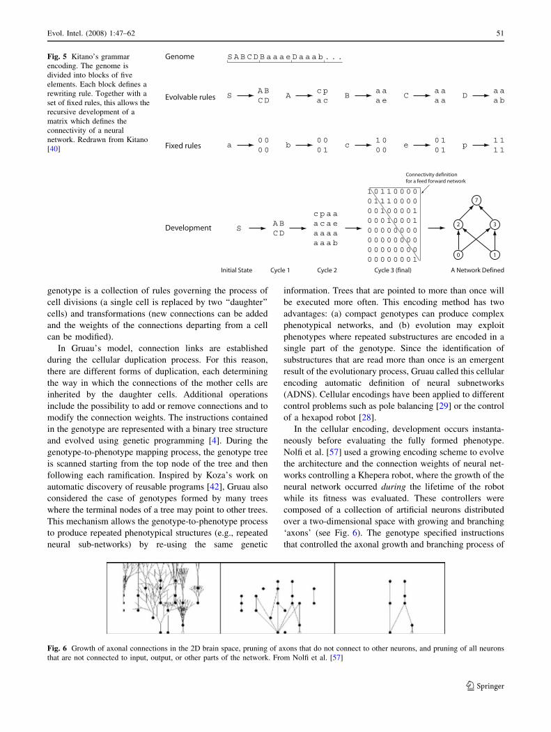
Nolfi et al. [57] used a growing encoding scheme to evolve

the architecture and the connection weights of neural net-

works controlling a Khepera robot, where the growth of the

neural network occurred during the lifetime of the robot

while its fitness was evaluated. These controllers were

composed of a collection of artificial neurons distributed

over a two-dimensional space with growing and branching

‘axons’ (see Fig. 6). The genotype specified instructions

that controlled the axonal growth and branching process of

Fig. 5 Kitano’s grammar

encoding. The genome is

divided into blocks of five

elements. Each block defines a

rewriting rule. Together with a

set of fixed rules, this allows the

recursive development of a

matrix which defines the

connectivity of a neural

network. Redrawn from Kitano

[40]

Fig. 6 Growth of axonal connections in the 2D brain space, pruning of axons that do not connect to other neurons, and pruning of all neurons

that are not connected to input, output, or other parts of the network. From Nolfi et al. [57]

Evol. Intel. (2008) 1:47–62 51

123

a set of neurons. When the axon growing from one neuron

reached another neuron, a connection between the two

neurons was established. Axons grew and branched only if

the neurons displayed an activation variability above a

genetically specified threshold. Axons that did not connect

to other neurons and neurons that remained unconnected

were pruned.

This activity-dependent growth was based on the idea

that the sensory information coming from the environment

plays a critical role in the maturation of the connectivity of

the biological nervous system. Indeed, it has been shown

that the maturation process is affected by the activity pat-

terns of single neurons [59, 60]. The developmental process

of these individuals was therefore determined both by

genetic and by environmental factors.

Husbands et al. [36] proposed a similar method where

the connections grew according to a set of differential

equations. The genotype encoded the properties of each

neuron (the type of neuron, the relative position with respect

to the neuron created previously, the initial direction of

growth of the dendrites and the parameters of the equations

governing the growth process). During the genotype-to-

phenotype process, the genetic string was scanned from left

to right until a particular marker was found. When a special

marker indicating the beginning of the description of a

neuron was encountered, the following bits were read and

interpreted as parameters for a new neuron. The presence of

an additional marker, however, could indicate that the

parameters of the current neuron were specified in a pre-

vious portion of the string. This mechanism could

potentially allow the emergence of phenotypes with repe-

ated structures formed by re-expression of the same genetic

instructions, similarly to the approach described by Gruau.

Despite the ability of developmental approaches to

generate large networks from compact genetic representa-

tions, it is not clear to what extent the network size

contributes to solve a problem. Developmental represen-

tations tend to generate regular and modular architectures,

which can be very suitable for problems that require them,

such as the control of a multi-legged robot. However, these

methods require additional mechanisms to cope with

asymmetric architectures and fine-tuning of specific

parameters.

2.3 Implicit encoding

A recent approach to representing neural networks is

inspired from the mechanisms of biological gene regula-

tory networks (GRNs). The so-called implicit encoding is

frequently used as a representation for GRN models [10]

and has also been considered as a representation for other

types of networks, such as neural networks.

In biological gene networks, the interaction between the

genes is not explicitly encoded in the genome, but follows

implicitly from the physical and chemical environment in

which the genome is immersed. The activation of a gene

results from interactions of proteins in the environment of

the gene with the so-called regulatory regions (see Fig. 7a).

These are sequences of nucleotides to which the proteins

can bind to promote or hinder the working of specialized

molecular machinery that is in charge of expressing the

gene. The expression of the gene corresponds to the syn-

thesis of proteins specified in another sequence of genetic

characters, the so-called coding region of the gene. The

start and end of the coding region of a gene are marked by

special motifs (i.e., nucleotide patters), called promoter

and terminator regions. The proteins produced by a gene

can in turn interact with the regulatory regions of other

genes and influence their expression. This process can

be interpreted as a network of interactions between the

different genes.

...XOVJWPGNBMJHDBTEOODFODDPWXXTEKCMRSIZZKJUWPOXCGNJJYXXVISTEVUBYCPTESSOOXI...

a

b

Fig. 7 a In biological gene

networks, the link between

genes is realized by molecules

that are synthesized from the

coding region of one gene and

interact with the regulatory

region of another gene.

b Analog genetic encoding

abstracts this mechanism with

an interaction map that

transforms the coding and

regulatory regions into a

numerical value that represents

the strength of the link. From

Mattiussi et al. [46]

52 Evol. Intel. (2008) 1:47–62

123

Reil [63, 64] studied the structural properties of such

gene networks with a simple computational model. He

used a sequence of characters from a finite alphabet as a

genome. The presence of a gene in the genome is sig-

naled by the presence of a promoter, that is, a predefined

sequence of fixed length. A gene is constituted by a fixed,

predefined number of characters following a promoter. In

Reil [63], an activated gene produces another sequence of

characters which is a transliterated version of the gene.

The new sequence is interpreted as a regulatory protein. If

a regulatory protein matches exactly a sequence of char-

acters in the genome, it regulates the expression of the

gene that immediately follows the matched genome

sequence (see Fig. 8). The regulation can be positive or

negative, and is of the on-off type, with repression pre-

vailing over activation. Geard and Wiles [25] refined this

model by complexifying the map that transforms a gene

into a regulator protein, adding a further level of regu-

lation which mimics the action of small RNA regulation

in real genomes and defining regulation in terms of a

weighted sum of regulator proteins effects. The simula-

tion of such artificial GRNs produced behaviors featuring

many properties observed in real GRNs. Although these

early computational GRN models were not directly aimed

at the exploitation of the evolutionary properties of such a

system, they inspired other researchers such as Bongard

[10] to use GRN models to evolve autonomous agents.

Bongard used a GRN model that relied on the diffusion of

chemicals, so-called transcription factors, which could

either directly influence the phenotype of the agent or

regulate the expression of genes. The results of his

computational experiments showed that his simple model

allowed for the evolution of complex morphologies

capable of simple locomotion behaviors and indicated that

the evolution of modular GRNs was beneficial for the

success of the agents.

This type of abstraction of the biochemical process of

gene regulation can be extended to a genetic representation

for any kind of analog network.1 Analog genetic encoding

(AGE) is such a representation which has been applied to

the evolution of ANNs [15, 44, 46]. AGE is based on a

discrete genome composed of sequences of characters from

a finite alphabet (e.g., the ASCII uppercase alphabet) which

is decoded into a network of interconnected devices (see

Fig. 7b). In the case of an artificial neural network, the

different types of neurons of the network are encoded by

sequences of genome which are separated by predefined

delimiter sequences. These artificial coding and regulatory

regions play a role analogous to the corresponding

sequences in biological genomes.

The biochemical process which determines the interac-

tion between the proteins encoded by one gene and the

regulatory region of another gene is abstracted by the so-

called interaction map. The interaction map is a mathe-

matical function that takes two sequences of characters as

argument and outputs a numerical value representing the

synaptic weight between two neurons. The neural network

can be decoded from the genome by scanning it for the

sequences of characters which represent a neuron. Subse-

quently, the interaction map can be used to compute the

interaction strengths between these neurons (see Fig. 9).

The size and topology of the decoded network hence

depends on the number of neurons encoded in the genome

and the interaction strengths between them (which can be

zero, thus leading to no connection between the corre-

sponding neurons).

In AGE, the sequences that define the interaction

between devices can have variable length, and the inter-

action map that is used to establish the connection between

the neurons is defined so as to apply to sequences of

arbitrary length. The assemblies of sequences of characters

that represent a neuron can be located anywhere in the

genome and can be spaced by stretches of non-coding

genetic characters. In this way the structure of the genome

Fig. 8 A simple model of gene expression and regulation in artificial

genomes. The genes which are marked by promoter regions in the

genome, are translated into transcription factors. These transcription

factors are then used to regulate the expression of the following genes.

Redrawn from Reil [64]

1 Analog networks are collections of dynamical devices intercon-

nected by links of varying strength. For example, genetic regulatory

networks, metabolic networks, neural networks, or electronic circuits

can be seen as analog networks.

Evol. Intel. (2008) 1:47–62 53

123

is not unduly constrained and tolerates a large class of

genetic operators, which can alter both the topology and

the sizing of the encoded network. In particular, the AGE

genome permits the insertion, deletion and substitution of

single characters, and the insertion, deletion, duplication,

and transposition of whole genome fragments. All these

genetic mutations are known to occur in biological gen-

omes and to be instrumental to their evolution. In

particular, gene duplication and the insertion of fragments

of genome of foreign organisms are deemed to be crucial

mechanism for the evolutionary increase of complexity of

GRNs [75]. Finally, the interaction map is defined so as to

be highly redundant, so that many different pairs of char-

acter sequences produce the same numeric value. Thus,

many mutations have no effect, resulting potentially in a

high neutrality in the search space.

When compared to NEAT, AGE reported equal per-

formance on a non-Markovian double-pole balancing

problem [16], while both algorithms performed better than

a developmental encoding (CE) and a coevolution method

(ESP). However, both AGE and NEAT performed worse

than an evolution strategy with direct encoding of a fixed

topology ANN [38]. This indicates that if a suitable

topology is known in advance, it is better to use simpler

representations. Reisinger and Miikkulainen [65] showed

that an implicit encoding very similar to AGE outperforms

NEAT on a complex board-game task.

3 Neuroevolution with dynamic neuron models

Some applications, for example the detection or generation

of time sequences, require a dynamic behavior of the

neural networks. Feedback connections in ANNs with

static transfer functions can provide such dynamics.

Another possibility is the integration of dynamic neuron

models. Dynamic neural networks are more difficult to

train with learning algorithms that use gradient descent,

correlation, and reinforcement learning. Artificial evolution

instead has been used with success on a variety of appli-

cations because it can discover suitable architectures, time

constants and even learning algorithms.

3.1 Continuous-time recurrent neural networks

One of the most widely-used dynamic neuron models is

called continuous-time recurrent neural network, or

CTRNN [7]. In this model, the neural network can be seen

as a set of differential equations

dxiðtÞdt¼ 1

si�xiðtÞ þ

XN

j¼1

wijr xjðtÞ þ hj

� �þ Ii

!

i ¼ 1; 2; :::;N

ð1Þ

where xi(t) is the activation of neuron i at the time t, N is

the number of neurons in the network, si is a time constant

whose magnitude (for si [ 0) is inversely proportional to

the decay rate of the activation, wij is the connection weight

between neuron i and neuron j, r(x) = 1/(1 + e-x) is the

standard logistic activation function, hj is a bias term and Ii

represents an external input. CTRNNs display rich

dynamics and represent a first approximation of the time-

dependent processes that occur at the membrane of bio-

logical neurons. Sometimes these models are also called

leaky integrators, with reference to electrical circuits,

Fig. 9 A simple artificial neural

network represented with

analog genetic encoding. The

interaction strengths are

computed by the interaction

map I which takes sequences of

characters of arbitrary length as

arguments

54 Evol. Intel. (2008) 1:47–62

123

because the equation describing the neuron activation is

equivalent to that describing the voltage difference of a

capacitor, where the time constant of the exponential and

synaptic weights can be approximated by a set of resistors

[31]. While being one of the simplest nonlinear, continuous

dynamic network models, CTRNNs are universal dynamic

approximators [24]. This means that they can approximate

the trajectories of any smooth dynamical system arbitrarily

well for any finite interval of time.

Evolution of CTRNNs has been applied to difficult

problems such as robot control [86]. An interesting prop-

erty of CTRNNs is that they can display learning behavior

without synaptic plasticity because they can store inter-

mediate states in the activation function of internal

neurons. For example, Yamauchi and Beer [90] evolved

CTRNNs capable of generating and learning short

sequences without synaptic plasticity. Blynel and Floreano

[9] evolved a recurrent neural architecture capable of

reinforcement learning-like behaviors for a robot required

to navigate a T-maze.

3.2 Spiking neuron models

Most biological neurons communicate through action

potentials, or spikes, which are punctual events that result

from a process taking place at the output of the neuron.

In spiking neurons the activation state, which corre-

sponds to an analog value, can be approximated by the

firing rate of the neuron. That is, a larger number of spikes

within a given time window would be an indicator of

higher activation of the neuron. However, if that is the

case, it means that spiking neurons require relatively longer

time to communicate information to post-synaptic neurons.

This hints at the fact that spiking neurons may use other

ways to efficiently encode information, such as the firing

time of single spikes or the temporal coincidence of spikes

coming from multiple sources [77, 67]. It may therefore be

advantageous for engineering purposes to use models of

spiking neurons that exploit firing time in order to encode

spatial and temporal structure of the input patterns with less

computational resources.

There are several models of spiking neurons that

describe in detail the electrochemical processes that pro-

duce spiking events by means of differential equations

[34]. A simple way of implementing a spiking neuron is to

take the dynamic model of a CTRNN neuron and substitute

the output function with an element that compares the

neuron activation with its threshold followed by a pulse

generator that takes the form of a Dirac function (see

Fig. 10). In other words, if the neuron activation is larger

than the threshold, a spike is emitted. In order to prevent

continuous spike emission, one must also add a strong

negative feedback so that the neuron activation goes below

threshold immediately after spike emission. This model is

known as an Integrate and Fire neuron.

Korkin et al. [41] evolved spiking neural networks

which could produce time-dependent waveforms, such as

sinusoids. Floreano and Mattiussi [19] evolved networks of

spiking neurons for solving a non-trivial vision-based

navigation task. They compared a neural network using the

spike response model [26] with a conventional sigmoid

network which could not solve the problem. The authors

suggest that the intrinsic dynamics of the spiking neural

networks might provide more degrees of freedom that can

be exploited by evolution to create viable controllers.

Saggie et al. [70] compared spiking neural networks with

conventional static ANNs in a simple setup where an agent

had to search food and avoid poison in a simulated grid

world. Their results indicate that for tasks with memory

dependent dynamics, spiking neural networks can provide

less complex solutions. Federici [17] combined an integrate

and fire neuron model with a correlation-based synaptic

plasticity model and a developmental encoding. His results

from experiments with a simple robot navigation task

indicate that such a system may allow for the efficient

evolution of large networks.

4 Evolution and learning

One of the main advantages of using evolutionary algo-

rithms for the design and tuning of neural networks is that

evolution can be combined with learning,2 as shown in this

section.

The combination of evolution and supervised learning

provides a powerful synergy between complementary

search algorithms [8]. For example, gradient-based learn-

ing algorithms such as back-propagation [68, 69] are

sensitive to the initial weight values, which may

Fig. 10 The integrate and fire neuron is a simple extension of the

CTRNN neuron. The weighted sum of the inputs is fed to an

integrator which is followed by a threshold function and a pulse

generator. If the neuron activation is larger than a threshold, a spike is

emitted

2 Algorithms which combine evolutionary search with some kinds of

local search are sometimes called memetic algorithms [53].

Evol. Intel. (2008) 1:47–62 55

123

significantly affect the quality of the trained network. In

this case, evolutionary algorithms can be used to find the

initial weight values of networks to be trained with back-

propagation. The fitness function is computed using the

residual error of the network after training with back-

propagation on a given task (notice that the final weights

after supervised training are not coded back into the

genotype, i.e., evolution is Darwinian, not Lamarckian).

Experimental results consistently indicate that networks

with evolved initial weights can be trained significantly

faster and better (by two orders of magnitude) than net-

works with random initial weights. The genetic string can

also encode the values of the learning rate and of other

learning parameters, such as the momentum in the case of

back-propagation. In this case, Belew et al. [8] found that

the best evolved networks employed learning rates ten

times higher than values suggested before (i.e., much less

than 1.0), but this result may depend on several factors,

such as the order of presentation of the patterns, the

number of learning cycles allowed before computing the

fitness, and the initial weight values.

Evolutionary algorithms have been employed also to

evolve learning rules. In its general form, a learning rule can

be described as a function U of few variables, such as pre-

synaptic activity xi, postsynaptic activity yj, the current value

of the synaptic connection wij, and the learning signal tj

Dwij ¼ U xj; yi;wij; ti� �

ð2Þ

Chalmers [11] suggested to describe this function as a

linear combination of the products between the variables

weighted by constants. These constants are encoded in a

genetic string and evolved. The neural network is trained

on a set of tasks using the decoded learning rule and its

performance is used to compute the fitness of the corre-

sponding learning rule. The initial synaptic weights are

always set to small random values centered around zero.

Chalmers employed a fitness function based on the mean

square error. A neural network with a single layer of

connections was trained on eight linearly separable clas-

sification tasks. The genetic algorithm evolved a learning

rule similar to the delta rule by Widrow and Hoff [89].

Similar results were obtained by Fontanari and Meir [23].

Dasdan and Oflazer [14] employed a similar encoding

strategy as Chalmers to evolve unsupervised learning

rules for classification tasks. The authors reported that

evolved rules were more powerful than comparable,

human-designed rules. Baxter [6] encoded both the

architecture and whether a synapse could be modified by

a simple Hebb rule (the rule was predetermined). Flor-

eano and Mondada [20] allowed evolution to choose

among four Hebbian learning rules for each synaptic

connection and evaluated the approach for a mobile robot

requested to solve a sequential task involving multiple

sensory modalities and environmental landmarks. The

results indicated that the evolved robots had the ability to

adapt on-the-fly to changed environmental conditions

(including spatial reorganization, textures and even robot

morphologies) without incremental evolution [87]. On the

contrary, evolved neural networks with fixed weights

could not adapt to those changed conditions. Floreano

and Urzelai [22] also showed that a morphogenetic

approach can greatly benefit from co-evolution of syn-

aptic plasticity because the strengths of the growing

connections are developed by learning rules that are co-

evolved with the developmental rules. Finally, Floreano

and Urzelai [21] showed that dynamic environments

favor the genetic expression of plastic connections over

static connections.

DiPaolo [15] evolved spiking neural controllers mod-

eled using the Spike Response Model and heterosynaptic

variants of a learning rule called spike-timing dependent

plasticity (STDP) for a robot. The learning rule was

described as a polynomial expression of the STDP rule

where the components of the rule were weighted by indi-

vidual constants that were genetically encoded and evolved

(similar to the encoding proposed by Chalmers). The

author showed that evolved robots were capable of learning

suitable associations between environmental stimuli and

behavior.

Nolfi and Parisi [56] evolved a neural controller for a

mobile robot whose output layer included two ‘‘teaching

neurons’’ that were used to modify the connection weights

from the sensory neurons to the motor neurons with back-

propagation learning during the robot’s lifetime. This

special architecture allows for using the sensory informa-

tion not only to generate behavior but also to generate

teaching signals that can modify the behavior. Analysis of

the evolved robots revealed that they developed two dif-

ferent behaviors that were adapted to the particular

environment where they happened to be ‘‘born’’. The

evolved networks did not inherit an effective control

strategy, but rather a predisposition to learn to control. This

predisposition to learn involved several aspects such as a

tendency to move so as to experience useful learning

experiences and a tendency to acquire useful adaptive

characters through learning [56].

It has been known for a long time that learning may

affect natural evolution [3]. Empirical evidence shows that

this is the case also for artificial evolution when combined

with some form of learning [55]. Hinton and Nowlan [33]

proposed a simple computational model that shows how

learning might facilitate and guide evolution. They con-

sidered the case where a neural network confers added

reproductive fitness on an organism only if it is connected

in exactly the right way. In this worst case, there is no

reasonable path toward the good network and a pure

56 Evol. Intel. (2008) 1:47–62

123

evolutionary search can only discover which of the

potential connections should be present by trying possi-

bilities at random. In the words of the authors, the good

network is ‘‘like a needle in a haystack’’. Hinton and

Nowlan’s results suggest that the addition of learning

produces a smoothing of the fitness surface area around the

good combination of genes (weights), which can be dis-

covered and easily climbed by the genetic algorithm (see

Fig. 11).

One of the main limitations of Hinton and Nowlan’s

model is that the learning space and the evolutionary space

are completely correlated.3 By systematically varying the

cost of learning and the correlation between the learning

space and the evolutionary space, Mayley [47] showed

that: (1) the adaptive advantage of learning is proportional

to the correlation between the two search spaces; (2) the

assimilation of characters first acquired through learning is

proportional to the correlation between the two search

spaces and to the cost of learning (i.e., to the fitness lost

during the first part of the lifetime in which individuals

have suboptimal performance); (3) in certain situations

learning costs may exceed learning benefits.

In the computational literature, it is sometimes debated

whether Lamarckian evolution (i.e., an evolutionary pro-

cess where characters acquired through learning are

directly coded back into the genotype and transmitted to

offspring) could be more effective than Darwinian evolu-

tion (i.e., an evolutionary process in which characters

acquired through learning are not coded back into the

genotype). Ackley and Littman [1] for instance claimed

that in artificial evolution, where inherited characters can

easily be coded into the genotype given that the mapping

between genotype and phenotype is generally quite simple,

it is preferable to use Lamarckian evolution. Indeed the

authors showed that Lamarckian evolution is far more

effective than Darwinian evolution in a stationary envi-

ronment (where the input-output mapping does not

change). However, Sasaki and Tokoro [71] showed that

Darwinian evolution largely outperforms Lamarckian

evolution when the environment is not stationary or when

different individuals are exposed to different learning

experiences.

5 Evolution of learning architectures

Experimental data suggests that mammalian brains employ

learning mechanisms that result in behaviors similar to

those produced by Reinforcement learning [50, 74].

Reinforcement learning is a class of learning algorithms

that attempts to estimate explicitly or implicitly the value

of the states experienced by the agents in order to favor the

choice of those actions that maximize the amount of

positive reinforcement received by the agent over time

[84]. The exact mechanism that implements this kind of

learning in biological neural system is the subject of

ongoing research and is not yet completely understood. The

existing evidence points to the combined action of evolved

value systems [58] and neuromodulatory effects [2, 18].

The value system has the task of discriminating the

behaviors according to their reinforcing, punishing, or

negligible consequences. This leads to the production of

neuromodulatory signals that can activate or inhibit syn-

aptic learning mechanisms.

Algorithms inspired by this approach have been devel-

oped by the machine learning community. The actor-critic

model [5, 83] for example, is a simple neural architecture

that implements reinforcement learning with two modules,

the Actor and the Critic shown in Fig. 12. Both modules

receive information on the current sensory state. In addi-

tion, the Critic receives information on the current

reinforcement value (external reinforcement) from the

environment. The output of the Critic generates an estimate

of the weighted sum of future rewards. The output of the

Actor instead is a probability of executing a certain set of

actions. This allows the system to perform an exploration

of the state-action space.

Typically such models are implemented in ANNs with a

fixed architecture where separate modules realize the

sensory preprocessing, the value system and the action-

Fig. 11 Fitness landscape with and without learning. In absence of

learning, the fitness landscape is flat, with a thin spike in correspon-

dence of the good combinations of genes (thick line). When learning

is enabled (dotted line), the fitness surface displays a smooth hill

around the spike corresponding to the gene combination which have

in part correct fixed values and in part unspecified (learnable) values.

Redrawn from Hinton and Nowlan [33]

3 The two spaces are correlated if genotypes which are close in the

evolutionary space correspond to phenotypes which are also close in

the phenotype space.

Evol. Intel. (2008) 1:47–62 57

123

selection mechanism.4 This puts the load of finding the

optimal structure of the value and the action-selection

system on the human designer. The integration of neuro-

modulation into a neuroevolution framework, as described

in the next section, allows for the evolution of reinforce-

ment learning-like architectures without any human

intervention.

5.1 Evolution of neuromodulatory architectures

In biological organisms, specialized neuromodulatory

neurons control the amount of activity-dependent plasticity

in the connection strength of other neurons. This effect is

mediated by special neurotransmitters called neuromodu-

lators [39]. Well known neuromodulators are e.g.,

dopamine, serotonine, noradrenaline and acetylcholine. A

simple model of neuromodulation can easily be integrated

into a conventional neuroevolution framework by intro-

ducing a second type of neuron. These modulatory neurons

affect the learning events at the postsynaptic site (see

Fig. 13). However, the implementation of such an

approach requires a genetic representation that allows for

the evolution of neural architectures consisting of several

different types of neurons. In Soltoggio et al. [78] this has

been realized using Analog Genetic Encoding (see

Sect. 2.3) and a parameterized, activity dependent Hebbian

learning model [54]. The authors show how reinforcement-

learning like behavior can evolve in a simulated foraging

experiment. A simulated bee has to collect nectar on a field

that contains two types of flowers (see Fig. 14). As the

amount of nectar associated with each of the flowers

changes stochastically, the behavioral strategy to maximize

the amount of collected nectar has to be adapted. The

evolved networks (see Fig. 15) implemented a value-based

learning strategy which was found to generalize to sce-

narios different from those used to assess the quality of the

solution during evolution, outperforming the results

obtained with hand-designed value-based learning archi-

tectures [78].

Another approach to evolving neuromodulatory archi-

tectures was suggested by Husbands et al. [37]. They

developed and evolved a class of neural networks called

GasNets, inspired by the modulatory effects of freely dif-

fusing gases, such as nitric oxide, which affect the response

profile of neurons in biological neural networks. In Gas-

Nets, some of the neurons, which are spatially distributed

over a 2D surface, emit ‘gases’ that diffuse through the

network and modulate the profile of the activation function

of other neurons in their vicinity. The spatial distance

between the neurons determines both the gas concentration

(as a result of the diffusion dynamics) and, in combination

with additional genetic parameters, the network

connectivity.

The authors showed that the modulation caused by gas

diffusion introduces a form of plasticity in the network

without synaptic modification. A comparison with con-

ventional neural networks in a robot control task indicated

better evolvability of the GasNets [37]. In another set of

experiments, McHale and Husbands [48] compared Gas-

Nets to CTRNNs and conventional ANNs with Hebbian

learning in a robot locomotion control tasks. From all

Fig. 12 The Actor–Critic architecture for reinforcement learning.

Redrawn from Mizutani and Dreyfus [49]

mod

n1 n2

Fig. 13 Neuromodulatory neurons permit the implementation of a

value-based learning mechanism in artificial neural networks. The

basic learning mechanism changes the weight of the link between the

two neurons n1 and n2 according to their activity. The neuromodu-

latory neuron mod modulates (i.e., strengthens or suppresses) the

basic learning mechanism and permits the synthesis of networks

where the learning is activated only in particular circumstances. From

Mattiussi et al. [46]

4 An alternative approach to this are neural learning classifiersystems. For example, Hurst and Bull [35] addressed the control of a

simulated robot in a maze task. They used a population of neural

networks acting as ‘rules’ controlling the robot. As evolution favored

rules that led to succesful behavior, the set of rules adapted to the

requirements of the task.

58 Evol. Intel. (2008) 1:47–62

123

tested networks, only the GasNets achieved a cyclic loco-

motion, but the CTRNNs achieved a higher average fitness.

This is in line with Magg and Philippides [43] whose

results indicate that GasNets perform extremely well on

tasks that require some kind of neural pattern generator or

timer, while performing worse on tasks which do not

require different time scales in the network.

6 Closing remarks

The methods for evolving neural networks have greatly

advanced over the years. In particular, we have witnessed a

significant progress in the ability to evolve architectures

and learning for dynamic neural networks, which are very

powerful systems for real-world problems such as robot

control.

From a practical point of view, artificial evolution turns

out to be extremely efficient, or even unique, when it is

used to explore both the topology and the adaptive prop-

erties of neural networks because other training algorithms

usually require stronger assumptions and constraints on the

choice of architecture, training data distribution, and opti-

mization function. Although there are no rigorous

comparisons between alternative methods, this claim is

supported by the fact that most experiments reported in the

literature with neural robots in real environments resort to

some sort of evolutionary procedure rather than to other

types of training algorithms.

From a scientific point of view, artificial evolution can

be used to test hypothesis of brain development and

dynamics because it can encompass multiple temporal and

spatial scales along which an organism evolves, such as

genetic, developmental, learning, and behavioral phenom-

ena. The possibility to co-evolve both the neural system

and the morphological properties of agents (although this

latter aspect is not reviewed in this paper) adds an addi-

tional valuable perspective to the evolutionary approach

that cannot be matched by any other approach.

We think that neuroevolution will continue to provide

efficient solutions to hard problems as well as new insights

into how biological brains became what they are in phys-

ical bodies interacting with dynamic environments. Within

this context, we believe that the evolution of neural

architectures with elements that gate or modulate learning

will generate novel understanding of reinforcement-learn-

ing like structures that are so important for biological and

robotic life.

Acknowledgements This work was supported by the Swiss

National Science Foundation, grant no. 200021-112060. Thanks to

Daniel Marbach for the illustrations and the two anonymous

reviewers for their helpful comments.

References

1. Ackley DH, Littman ML (1992) Interactions between learning

and evolution. In: Langton C, Farmer J, Rasmussen S, Taylor C

(eds) Artificial Life II: Proceedings volume of Santa Fe confer-

ence, vol XI. Addison Wesley, Redwood City, pp 487–510

2. Bailey CH, Giustetto M, Huang Y.-Y, Hawkins RD, Kandel ER

(2000) Is heterosynaptic modulation essential for stabilizing

Hebbian plasticity and memory? Nat Rev Neurosci 1(1):11–20

Fig. 14 A simulated bee with a simple vision system flies over a field

containing patches of blue and yellow flowers, represented here as

dark and light squares. The quality of the behavior of the simulated

bee is judged from the amount of nectar that the bee is able to collect

in a series of landings. From Soltoggio et al. [78]

Fig. 15 An example of a neuromodulatory network evolved with

analog genetic encoding, which solves the foraging task of Fig. 14.

The G, B, and Y squares represent the color inputs of the visual

system. The R square represents the reward input that gives the

amount of nectar found on the flower on which the simulated bee has

landed. The landing is signaled by the activation of the input L. The

square denoted by 1 represents a fixed value input (bias), and the dG,

dB, dY inputs represent the memory of the color observed just before

landing. The dG, dB, and dY input signals were defined because they

were used in experiments with hand-designed neural architectures for

the same scenario [54]. The figure shows that these inputs were found

by the algorithm to be not necessary to solve the task and were thus

left unconnected at the end of the evolutionary search. In the network

shown here, the neuromodulatory mod neuron modulates the learning

of all the connections between the inputs and the output neuron. From

Soltoggio et al. [78]

Evol. Intel. (2008) 1:47–62 59

123

3. Baldwin JM (1896) A new factor in evolution. Am Nat 30:441–

451

4. Banzhaf W, Nordin P, Keller RE, Francone FD (1998) Genetic

programming—an introduction. In: On the automatic evolution of

computer programs and its applications. Morgan Kaufmann, San

Francisco

5. Barto AG (1995) Adaptive critic and the basal ganglia. In: Houk

JC, Davis JL, Beiser DG (eds) Models of information processing

in the basal ganglia. MIT Press, Cambridge, pp 215–232

6. Baxter J (1992) The evolution of learning algorithms for artificial

neural networks. In: Green D, Bossomaier T (eds) Complex

Systems. IOS Press

7. Beer RD, Gallagher JC (1992) Evolving dynamical neural net-

works for adaptive behavior. Adapt Behav 1:91–122

8. Belew RK, McInerney J, Schraudolph NN (1992) Evolving net-

works: using the genetic algorithm with connectionistic learning.

In: Langton CG, Taylor C, Farmer JD, Rasmussen S (eds) Pro-

ceedings of the 2nd Conference on Artificial Life. Addison-

Wesley, Reading, pp 511–548

9. Blynel J, Floreano D (2003) Exploring the T-maze: evolving

learning-like robot behaviors using CTRNNs. In: Raidl Ge AE

(ed) 2nd European workshop on evolutionary robotics

(EvoRob’2003)

10. Bongard J (2002) Evolving modular genetic regulatory networks.

In: Proceedings of the 2002 congress on evolutionary computa-

tion 2002, CEC ’02, vol 2, pp 1872–1877

11. Chalmers DJ (1990) The evolution of learning: an experiment in

genetic connectionism. In: Touretzky DS, Elman JL, Sejnowski

T, Hinton GE (eds) Proceedings of the 1990 connectionist models

summer school. Morgan Kaufmann, San Mateo, pp 81–90

12. Chandra A, Yao X (2006) Ensemble learning using multi-

objective evolutionary algorithms. J Math Model Algorithms

5(4):417–445

13. Chellapilla K, Fogel D (2001) Evolving an expert checkers

playing program without using humanexpertise. IEEE Trans Evol

Comput 5(4):422–428

14. Dasdan A, Oflazer K (1993) Genetic synthesis of unsupervised

learning algorithms. In: Proceedings of the 2nd Turkish sympo-

sium on artificial intelligence and ANNs. Department of

Computer Engineering and Information Science, Bilkent Uni-

versity, Ankara

15. DiPaolo E (2003) Evolving spike-timing-dependent plasticity for

single-trial learning in robots. Phil Trans R Soc Lond A

361:2299–2319

16. Durr P, Mattiussi C, Floreano D (2006) Neuroevolution with

Analog Genetic Encoding. In: Parallel problem solving from

nature—PPSN iX, vol 9. Springer, Berlin, pp 671–680

17. Federici D (2005) Evolving developing spiking neural networks.

In: Proceedings of CEC 2005 IEEE congress on evolutionary

computation

18. Fellous J-M, Linster C (1998) Computational models of neuro-

modulation. Neural Comput 10(4):771–805

19. Floreano D, Mattiussi C (2001) Evolution of spiking neural

controllers for autonomous vision-based robots. In: Gomi T (ed)

Evolutionary robotics. From intelligent robotics to artificial life.

Springer, Tokyo

20. Floreano D, Mondada F (1996) Evolution of plastic neurocon-

trollers for situated agents. In: Maes P, Mataric M, Meyer J,

Pollack J, Roitblat H, Wilson S (eds) From animals to animats

IV: proceedings of the 4th international conference on simulation

of adaptive behavior. MIT Press-Bradford Books, Cambridge, pp

402–410

21. Floreano D, Urzelai J (2000) Evolutionary robots with online

self-organization and behavioral fitness. Neural Netw 13:431–443

22. Floreano D, Urzelai J (2001) Evolution of plastic control net-

works. Autonom Robots 11(3):311–317

23. Fontanari JF, Meir R (1991) Evolving a learning algorithm for the

binary perceptron. Network 2:353–359

24. Funahashi K, Nakamura Y (1993) Approximation of dynamical

systems by continuous time recurrent neural networks. Neural

Netw 6(6):801–806

25. Geard NL, Wiles J (2003) Structure and dynamics of a gene

network model incorporating small RNAs. In: Proceedings of

2003 congress on evolutionary computation, pp 199–206

26. Gerstner W (1999) Spiking neurons. In: Maass W, Bishop CM

(eds) Pulsed neural networks. MIT Press-Bradford Books,

Cambridge

27. Gomez F, Miikkulainen R (1997) Incremental evolution of

complex general behavior. Adapt Behav 5(3–4):317–342

28. Gruau F (1995) Automatic definition of modular neural networks.

Adapt Behav 3(2):151–183

29. Gruau, F, Whitley, D, and Pyeatt, L (1996) A comparison

between cellular encoding and direct encoding for genetic neural

networks. In: Koza JR, Goldberg DE, Fogel DB, Riolo RL (eds)

Genetic programming 1996: proceedings of the first annual

conference. MIT Press, Stanford University, pp 81–89

30. Hansen N, Ostermeier A (2001) Completely derandomized self-

adaptation in evolution strategies. Evol Comput 9(2):159–195

31. Haykin, S (1999) Neural networks. a comprehensive foundation,

2nd edn. Prentice Hall, Upper Saddle River

32. Hebb DO (1949) The organisation of behavior. Wiley, New York

33. Hinton GE, Nowlan SJ (1987) How learning can guide evolution.

Complex Syst 1:495–502

34. Hodgkin AL, Huxley AF (1952) A quantitative description of

membrane current and its application to conduction and excita-

tion in nerve. J Physiol (Lond) 108:500–544

35. Hurst J, Bull L (2006) A neural learning classifier system with

self-adaptive constructivism for mobile robot control. Artif Life

12 (3):353–380

36. Husbands P, Harvey I, Cliff D, Miller G (1994) The use of

genetic algorithms for the development of sensorimotor control

systems. In: Gaussier P, Nicoud J-D (eds) From perceptin to

action. IEEE Press, Los Alamitos

37. Husbands P, Smith T, Jakobi N, O’Shea M (1998) Better living

through chemistry: evolving gasnets for robot control. Connect

Sci 10:185–210

38. Igel, C (2003) Neuroevolution for reinforcement learning using

evolution strategies. In: Sarker R, et al (eds) Congress on evo-

lutionary computation, vol 4. IEEE Press, New York, pp 2588–

2595

39. Katz PS (1999) What are we talking about? Modes of neuronal

communication. In: Katz P (eds) Beyond neurotransmission:

neuromodulation and its importance for information processing,

chap 1. Oxford University Press, Oxford, pp 1–28

40. Kitano H (1990) Designing neural networks by genetic algo-rithms using graph generation system. Complex Syst J 4:461–

476

41. Korkin M, Nawa NE, de Garis H (1998) A ’spike interval

information coding’ representation for ATR’s CAM-brain

machine (CBM) In: Proceedings of the 2nd international con-

ference on evolvable systems: from biology to hardware

(ICES’98). Springer, Heidelberg

42. Koza JR (1994) Genetic programming II: automatic discovery of

reusable programs. MIT Press, Cambridge

43. Magg S, Philippides A (2006) Gasnets and CTRNNs : a com-

parison in terms of evolvability. In: From animals to animats 9:

proceedings of the 9th international conference on simulation of

adaptive behavior. Springer, Heidelberg, pp 461–472

44. Mattiussi C, Floreano D (2004) Evolution of analog networks

using local string alignment on highly reorganizable genomes. In:

Zebulum RS et al (eds) NASA/DoD conference on evolvable

hardware (EH’2004), pp 30–37

60 Evol. Intel. (2008) 1:47–62

123

45. Mattiussi C, Durr P, Floreano D (2007a) Center of mass encod-

ing: a self-adaptive representation with adjustable redundancy for

real-valued parameters. In: GECCO 2007. ACM Press, New

York, pp 1304–1311

46. Mattiussi C, Marbach D, Durr P, Floreano D (2007b) The age of

analog networks. AI Magazine (in press)

47. Mayley G (1996) Landscapes, learning costs and genetic assim-

ilation. Evol Comput 4(3):213–234

48. McHale G, Husbands P (2004) Gasnets and other evolvable

neural networks applied to bipedal locomotion. In: Schaal S (ed)

Proceedings from animals to animats 8: proceedings of the 8th

international conference on simulation of adaptive behaviour

(SAB’2004). MIT Press, Cambridge, pp 163–172

49. Mizutani E, Dreyfus SE (1998) Totally model-free reinforcement

learning by actor-critic elman networks in non-markovian

domains. In: Proceedings of the IEEE world congress on com-

putational intelligence. IEEE Press, New York

50. Montague P, Dayan P, Sejnowski T (1996) A framework for

mesencephalic dopamine systems based on predictive Hebbian

learning. J Neurosci 16(5):1936–1947

51. Montana D, Davis L (1989) Training feed forward neural net-

works using genetic algorithms. In: Proceedings of the 11th

international joint conference on artificial intelligence. Morgan

Kaufmann, San Mateo, pp 529–538

52. Moriarty DE, Miikkulainen R (1996) Efficient reinforcement

learning through symbiotic evolution. Machine Learn 22:11–32

53. Moscato P (1989) On evolution, search, optimization, genetic

algorithms and martial arts: towards memetic algorithms. In:

Technical report C3P 826, Pasadena

54. Niv Y, Joel D, Meilijson I, Ruppin E (2002) Evolution of rein-

forcement learning in uncertain environments: A simple

explanation for complex foraging behaviors. Adapt Behav

10(1):5–24

55. Nolfi S, Floreano D (1999) Learning and evolution. Auton Robots

7(1):89–113

56. Nolfi S, Parisi D (1996) Learning to adapt to changing environ-

ments in evolving neural networks. Adapt Behav 5(1):75–98

57. Nolfi S, Miglino O, Parisi D (1994) Phenotypic plasticity in

evolving neural networks. In: Gaussier P, Nicoud J-D (eds) From

perception to action. IEEE Press, Los Alamitos

58. Pfeifer R, Scheier C (1999) Understanding Intelligence. MIT

Press, Cambridge

59. Purves D (1994) Neural activity in the growth of the brain.

Cambridge University Press, Cambridge

60. Quartz S, Sejnowski TJ (1997) The neural basis of cognitive

development: a constructivist manifesto. Behav Brain Sci 4:537–

555

61. Radcliffe NJ (1991) Form an analysis and random respectful

recombination. In: Belew RK, Booker LB (eds) Proceedings of

the 4th international conference on genetic algorithms. Morgan

Kaufmann, San Mateo

62. Rechenberg I (1973) Evolutionsstrategie—Optimierung techni-

scher Systeme nach Prinzipien der biologischen Evolution.

Fommann-Holzboog, Stuttgart

63. Reil T (1999) Dynamics of gene expression in an artificial gen-

ome—implications for biological and artificial ontogeny. In:

Proceedings of the 5th European conference on artificial life, pp

457–466

64. Reil T (2003) On growth, form and computers. In: Artificial

genomes as models of gene regulation. Academic Press, London,

pp 256–277

65. Reisinger J, Miikkulainen R (2007) Acquiring evolvability

through adaptive representations. In: Proceedings of genetic and

evolutionary computation conference (GECCO 2007)

66. Reisinger J, Bahceci E, Karpov I, Miikkulainen R (2007) Coe-

volving strategies for general game playing. In: Proceedings of

the IEEE symposium on computational intelligence and games

(CIG-2007)

67. Rieke F, Warland D, van Steveninck R, Bialek W (1997) Spikes.

Exploring the neural code. MIT Press, Cambridge

68. Rumelhart DE, Hinton GE, Williams RJ (1986a) Learning rep-

resentations by back-propagation of errors. Nature 323:533–536

69. Rumelhart DE, McClelland J, the PDP Research Group (1986b)

Parallel distributed processing: explorations in the microstructure

of cognition. Foundations, vol 1. MIT Press-Bradford Books,

Cambridge

70. Saggie K, Keinan A, Ruppin E (2004) Spikes that count:

rethinking spikiness in neurally embedded systems. Neurocom-

puting 58-60:303–311

71. Sasaki T, Tokoro M (1997) Adaptation toward changing envi-

ronments: Why Darwinian in nature?. In: Husbands P, Harvey I

(eds) Proceedings of the 4th European conference on artificial

life. MIT Press, Cambridge

72. Schaffer JD, Whitley D, Eshelman LJ (1992) Combinations of

genetic algorithms and neural networks: a survey of the state of

the art. In: Whitley D, Schaffer JD (eds) Proceedings of an

international workshop on the combinations of genetic algorithms

and neural networks (COGANN-92). IEEE Press, New York

73. Schraudolph NN, Belew RK (1992) Dynamic parameter encoding

for genetic algorithms. Machine Learn 9:9–21

74. Schultz W, Dayan P, Montague PR (1997) A neural substrate of

prediction and reward. Science 275(5306):1593–1599

75. Shapiro J (2005) A 21st century view of evolution: genome

system architecture, repetitive DNA, and natural genetic engi-

neering. Gene 345(1):91–100

76. Siddiqi A, Lucas S (1998) A comparison of matrix rewriting

versus direct encoding for evolving neural networks. In: Pro-

ceedings of the 1998 IEEE international conference on

evolutionary computation. Piscataway, NJ, pp 392–397

77. Singer W, Gray CM (1995) Visual feature integration and the

temporal correlation hypothesis. Annu Rev Neurosci 18:555–

586

78. Soltoggio A, Duerr P, Mattiussi C, Floreano D (2007) Evolving

neuromodulatory topologies for reinforcement learning-like

problems. In: Angeline P, Michaelewicz M, Schonauer G, Yao X,

Zalzala Z (eds) Proceedings of the 2007 congress on evolutionary

computation. IEEE Press, New York

79. Stanley K, Miikkulainen R (2002) Evolving neural networks

through augmenting topologies. Evol Comput 10(2):99–127

80. Stanley KO, Miikkulainen R (2004) Competitive coevolution

through evolutionary complexification. J Artif Intell Res 21:63–

100

81. Stanley K, Kohl N, Sherony R, Miikkulainen R (2005a) Neuro-

evolution of an automobile crash warning system. In:

Proceedings of genetic and evolutionary computation conference

(GECCO 2005)

82. Stanley KO, Cornelius R, Miikkulainen R, D’Silva T, Gold A

(2005b) Real-time learning in the nero video game. In: Pro-

ceedings of the artificial intelligence and interactive digital

entertainment conference (AIIDE 2005) demo papers

83. Sutton RS (1988) Learning to predict by the method of temporal

difference. Machine Learn 3:9–44

84. Sutton RS, Barto AG (1998) Reinforcement learning. an intro-

duction. MIT Press, Cambridge

85. Trianni V, Ampatzis C, Christensen A, Tuci E, Dorigo M, Nolfi S

(2007) From solitary to collective behaviours: decision making

and cooperation. In: Advances in artificial life, proceedings of

ECAL 2007. Lecture Notes in Artificial Intelligence, vol LNAI

4648. Springer, Berlin, pp 575–584

86. Tuci E, Quinn M, Harvey I (2002) An evolutionary ecological

approach to the study of learning behavior using a robot-based

model. Adapt Behav 10(3–4):201–221

Evol. Intel. (2008) 1:47–62 61

123

87. Urzelai J, Floreano D (2001) Evolution of adaptive synapses:

robots with fast adaptive behavior in new environments. Evol

Comput 9:495–524

88. Whitley D, Starkweather T, Bogart C (1990) Genetic algorithms

and neural networks: optimizing connections and connectivity.

Parallel Comput 14:347–361

89. Widrow B, Hoff ME (1960) Adaptive switching circuits. In:

Proceedings of the 1960 IRE WESCON convention, vol IV, New

York. IRE. Reprinted in Anderson and Rosenfeld, 1988, pp 96–

104

90. Yamauchi BM, Beer RD (1994) Sequential behavior and learning

in evolved dynamical neural networks. Adapt Behav 2(3):219–

246

91. Yao X (1999) Evolving artificial neural networks. Proc IEEE

87(9):1423–1447

62 Evol. Intel. (2008) 1:47–62

123