HAL Id: hal-03090994https://hal.archives-ouvertes.fr/hal-03090994

Preprint submitted on 7 Jan 2021

HAL is a multi-disciplinary open accessarchive for the deposit and dissemination of sci-entific research documents, whether they are pub-lished or not. The documents may come fromteaching and research institutions in France orabroad, or from public or private research centers.

L’archive ouverte pluridisciplinaire HAL, estdestinée au dépôt et à la diffusion de documentsscientifiques de niveau recherche, publiés ou non,émanant des établissements d’enseignement et derecherche français ou étrangers, des laboratoirespublics ou privés.

Neuro-Steered Hearing Devices: Decoding AuditoryAttention From the Brain

Simon Geirnaert, Servaas Vandecappelle, Emina Alickovic, Alain deCheveigné, Edmund Lalor, Bernd T. Meyer, Sina Miran, Tom Francart,

Alexander Bertrand

To cite this version:Simon Geirnaert, Servaas Vandecappelle, Emina Alickovic, Alain de Cheveigné, Edmund Lalor, et al..Neuro-Steered Hearing Devices: Decoding Auditory Attention From the Brain. 2021. �hal-03090994�

1

Neuro-Steered Hearing DevicesDecoding Auditory Attention From the Brain

Simon Geirnaert, Servaas Vandecappelle, Emina Alickovic, Alain de Cheveigne,

Edmund Lalor, Bernd T. Meyer, Sina Miran, Tom Francart, and Alexander Bertrand

Abstract

People suffering from hearing impairment often have difficulties participating in conver-

sations in so-called ‘cocktail party’ scenarios with multiple people talking simultaneously.

Although advanced algorithms exist to suppress background noise in these situations, a hearing

device also needs information on which of these speakers the user actually aims to attend to.

Recent neuroscientific advances have shown that it is possible to determine the focus of auditory

attention from non-invasive neurorecording techniques, such as electroencephalography (EEG).

Based on these new insights, a multitude of auditory attention decoding (AAD) algorithms have

been proposed, which could, in combination with the appropriate speaker separation algorithms

and miniaturized EEG sensor devices, lead to a new generation of so-called neuro-steered hearing

devices. In this paper, we address the main signal processing challenges in this field and provide

a review and comparative study of state-of-the-art AAD algorithms.

I. INTRODUCTION

Current state-of-the-art hearing devices, such as hearing aids or cochlear implants, contain ad-

vanced signal processing algorithms to suppress acoustic background noise and as such assist the

constantly expanding group of people suffering from hearing impairment. However, situations

where multiple competing speakers are active at the same time (dubbed the ‘cocktail party

problem’) still cause major difficulties for the hearing device user, often leading to social isolation

and decreased quality of life. Beamforming algorithms that use microphone array signals to

This research is funded by an Aspirant Grant from the Research Foundation - Flanders (FWO) (for S. Geirnaert), the

KU Leuven Special Research Fund C14/16/057, FWO project nr. G0A4918N, the European Research Council (ERC)

under the European Unions Horizon 2020 research and innovation programme (grant agreement No 802895 and grant

agreement No 637424), and the Flemish Government under the Onderzoeksprogramma Artificile Intelligentie (AI)

Vlaanderen programme. The scientific responsibility is assumed by its authors.

The first two authors have implemented all the algorithms of the comparative study to ensure uniformity. All

implementations have been checked and approved by at least one of the authors of the original paper in which the

method was presented.

arX

iv:2

008.

0456

9v1

[ee

ss.S

P] 1

1 A

ug 2

020

2

suppress acoustic background noise and extract a single speaker from a mixture lack a fundamental

piece of information to assist the hearing device user in cocktail party scenarios: which speaker

should be treated as the attended speaker and which other speaker(s) should be treated as the

interfering noise sources? This issue is often addressed by using simple heuristics, such as look

direction or speaker intensity, which often fail in practice.

Recent neuroscientific insights on how the brain synchronizes with the speech envelope [1],

[2], have laid the groundwork for a new strategy to tackle this problem: extracting attention-

related information directly from the origin, i.e., the brain. This is generally referred to as the

auditory attention decoding (AAD) problem. In the last ten years, following these groundbreaking

advances in the field of auditory neuroscience and neural engineering, the topic of AAD has gained

traction in the biomedical signal processing community. In [3], a first successful AAD algorithm

was proposed based on electroencephalography (EEG), which is a non-invasive, wearable, and

relatively cheap neurorecording technique. The main idea is to decode the attended speech

envelope from a multi-channel EEG recording using a neural decoder and to correlate the decoder

output with the speech envelope of each speaker. Following this first AAD algorithm, a multitude

of new AAD algorithms have been proposed [4]–[10]. These advances could, in combination with

the appropriate blind speaker separation algorithms [11]–[15] and relying on rapidly evolving

improvements in miniaturization and wearability of EEG sensors [16]–[19], lead to a new assistive

solution for the hearing impaired: a neuro-steered hearing device.

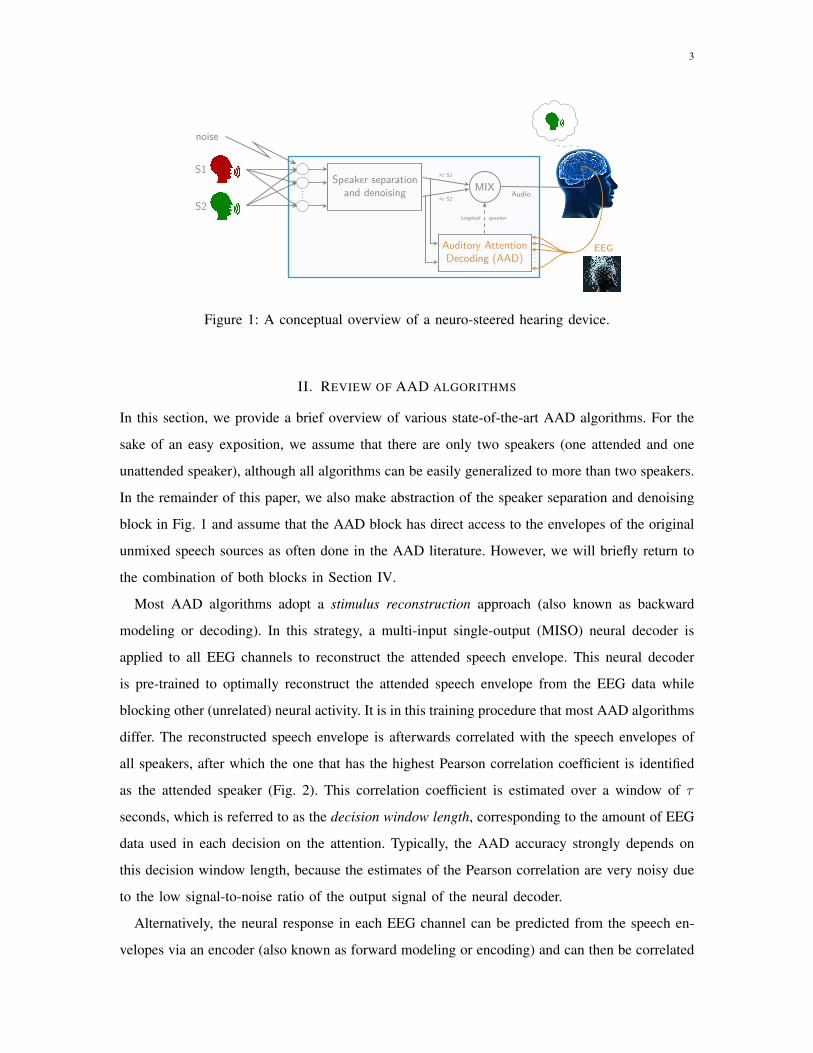
Fig. 1 shows a conceptual overview of a neuro-steered hearing device. The AAD block

contains an algorithm that determines the attended speaker by integrating the demixed speech

envelopes and the EEG. Despite the large variety in AAD algorithms, an objective and transparent

comparative study has not been performed to date, making it hard to identify which strategies are

most successful. In this paper, we will briefly review various state-of-the-art AAD algorithms and

provide an objective and quantitative comparative study using two independent publicly available

datasets [20], [21]. To ensure fairness and correctness, this comparative study has been reviewed

and endorsed by the author(s) of the original papers in which these algorithms were proposed.

While the main focus of this paper is on this AAD block, we also provide an outlook on other

practical challenges on the road ahead, such as the interaction of AAD with speech demixing or

beamforming algorithms and challenges related to EEG sensor miniaturization.

3

S1

S2

Speaker separationand denoising MIX

Auditory AttentionDecoding (AAD)

≈ S1

≈ S2

targeted speaker

EEG...

Audio

noise

Figure 1: A conceptual overview of a neuro-steered hearing device.

II. REVIEW OF AAD ALGORITHMS

In this section, we provide a brief overview of various state-of-the-art AAD algorithms. For the

sake of an easy exposition, we assume that there are only two speakers (one attended and one

unattended speaker), although all algorithms can be easily generalized to more than two speakers.

In the remainder of this paper, we also make abstraction of the speaker separation and denoising

block in Fig. 1 and assume that the AAD block has direct access to the envelopes of the original

unmixed speech sources as often done in the AAD literature. However, we will briefly return to

the combination of both blocks in Section IV.

Most AAD algorithms adopt a stimulus reconstruction approach (also known as backward

modeling or decoding). In this strategy, a multi-input single-output (MISO) neural decoder is

applied to all EEG channels to reconstruct the attended speech envelope. This neural decoder

is pre-trained to optimally reconstruct the attended speech envelope from the EEG data while

blocking other (unrelated) neural activity. It is in this training procedure that most AAD algorithms

differ. The reconstructed speech envelope is afterwards correlated with the speech envelopes of

all speakers, after which the one that has the highest Pearson correlation coefficient is identified

as the attended speaker (Fig. 2). This correlation coefficient is estimated over a window of τ

seconds, which is referred to as the decision window length, corresponding to the amount of EEG

data used in each decision on the attention. Typically, the AAD accuracy strongly depends on

this decision window length, because the estimates of the Pearson correlation are very noisy due

to the low signal-to-noise ratio of the output signal of the neural decoder.

Alternatively, the neural response in each EEG channel can be predicted from the speech en-

velopes via an encoder (also known as forward modeling or encoding) and can then be correlated

4

EEG decoder

envelope extraction

correlate over τ seconds ρ1

envelope extraction

correlate over τ seconds ρ2

max attendedspeaker

Figure 2: In the stimulus reconstruction approach, a decoder reconstructs the attended speech

envelope, which is correlated with the different speech envelopes to identify the attended speaker.

with the measured EEG [5], [22]. When the encoder is linear, this corresponds to estimating

impulse responses (aka temporal response functions) between the speech envelope(s) and the

recorded EEG signals. For AAD, backward MISO decoding models have been demonstrated to

outperform forward encoding models [5], [22], as the former can exploit the spatial coherence

across the different EEG channels at its input. In this comparative study, we thus only focus

on backward AAD algorithms, except for the canonical correlation analysis (CCA) algorithm

(Section II-A2), which combines both a forward and backward approach.

Due to the emergence of deep learning methods, a third approach has become popular: direct

classification [9], [10]. In this approach, the attention is directly predicted in an end-to-end

fashion, without explicitly reconstructing the speech envelope.

The decoder models are typically trained in a supervised fashion, which means that the attended

speaker has to be known for each data point in the training set. This requires the collection of

‘ground-truth’ EEG data during a dedicated experiment in which the subject is asked to pay

attention to a predefined speaker in a speech mixture. The models can be trained either in a

subject-specific fashion (based on EEG data from the actual subject under test) or in a subject-

independent fashion (based on EEG data from other subjects than the subject under test). The

latter leads to a universal (subject-independent) decoder, which has the advantage that it can be

applied to new subjects without the need to go through such a tedious ground-truth EEG data

collection for every new subject. However, since the brain responses of each person are different,

the accuracy achieved by such universal decoders is typically lower [3]. In this paper, we only

consider subject-specific decoders, which allows to achieve better accuracies, as they are tailored

to the EEG of the specific end-user.

5

AAD

algorithms

Nonlinear

Direct

classification

CNN-loc [10]

CNN-sim [9]

Stimulus

reconstructionNN-SR [8]

Linear

Direct

classificationNo algorithms yet

Stimulus

reconstruction

Training-free MMSE-adap-lasso [6]

Supervised

training

Forward

and backwardCCA [7]

Backward

Averaging

decoders

MMSE-avgdec-ridge [3]

MMSE-avgdec-lasso [5]

Averaging

autocorrelation

matrices

MMSE-avgcorr-ridge [4]

MMSE-avgcorr-lasso [5]

Contrast I (*)

Contrast II (*)

Contrast III (*)

Contrast IV (n.s.)

Contrast V (n.s.)

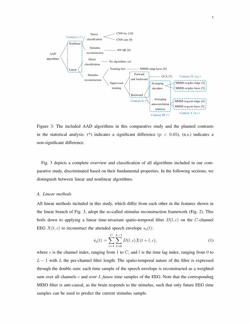
Figure 3: The included AAD algorithms in this comparative study and the planned contrasts

in the statistical analysis. (*) indicates a significant difference (p < 0.05), (n.s.) indicates a

non-significant difference.

Fig. 3 depicts a complete overview and classification of all algorithms included in our com-

parative study, discriminated based on their fundamental properties. In the following sections, we

distinguish between linear and nonlinear algorithms.

A. Linear methods

All linear methods included in this study, which differ from each other in the features shown in

the linear branch of Fig. 3, adopt the so-called stimulus reconstruction framework (Fig. 2). This

boils down to applying a linear time-invariant spatio-temporal filter D(l, c) on the C-channel

EEG X(t, c) to reconstruct the attended speech envelope sa(t):

sa(t) =

C∑c=1

L−1∑l=0

D(l, c)X(t+ l, c), (1)

where c is the channel index, ranging from 1 to C, and l is the time lag index, ranging from 0 to

L − 1 with L the per-channel filter length. The spatio-temporal nature of the filter is expressed

through the double sum: each time sample of the speech envelope is reconstructed as a weighted

sum over all channels c and over L future time samples of the EEG. Note that the corresponding

MISO filter is anti-causal, as the brain responds to the stimulus, such that only future EEG time

samples can be used to predict the current stimulus sample.

6

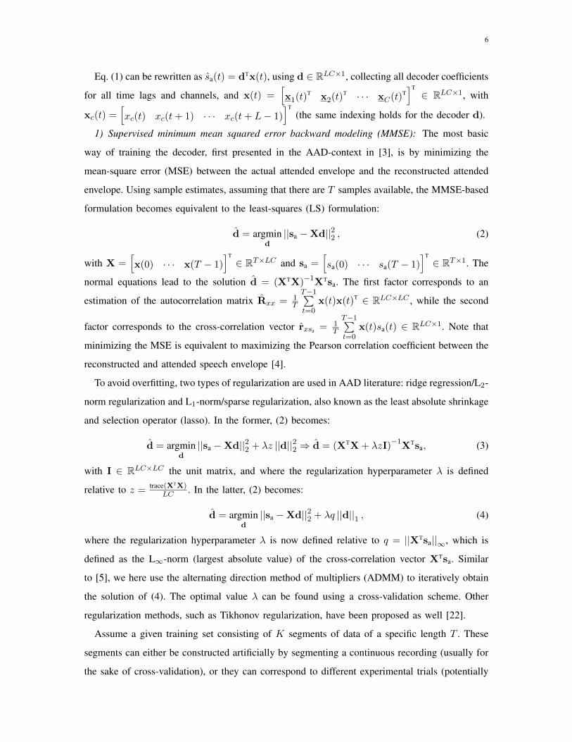
Eq. (1) can be rewritten as sa(t) = dTx(t), using d ∈ RLC×1, collecting all decoder coefficients

for all time lags and channels, and x(t) =[x1(t)

T x2(t)T · · · xC(t)

T]T

∈ RLC×1, with

xc(t) =[xc(t) xc(t+ 1) · · · xc(t+ L− 1)

]T

(the same indexing holds for the decoder d).

1) Supervised minimum mean squared error backward modeling (MMSE): The most basic

way of training the decoder, first presented in the AAD-context in [3], is by minimizing the

mean-square error (MSE) between the actual attended envelope and the reconstructed attended

envelope. Using sample estimates, assuming that there are T samples available, the MMSE-based

formulation becomes equivalent to the least-squares (LS) formulation:

d = argmind||sa −Xd||22 , (2)

with X =[x(0) · · · x(T − 1)

]T

∈ RT×LC and sa =[sa(0) · · · sa(T − 1)

]T

∈ RT×1. The

normal equations lead to the solution d = (XTX)−1XTsa. The first factor corresponds to an

estimation of the autocorrelation matrix Rxx = 1T

T−1∑t=0

x(t)x(t)T ∈ RLC×LC , while the second

factor corresponds to the cross-correlation vector rxsa = 1T

T−1∑t=0

x(t)sa(t) ∈ RLC×1. Note that

minimizing the MSE is equivalent to maximizing the Pearson correlation coefficient between the

reconstructed and attended speech envelope [4].

To avoid overfitting, two types of regularization are used in AAD literature: ridge regression/L2-

norm regularization and L1-norm/sparse regularization, also known as the least absolute shrinkage

and selection operator (lasso). In the former, (2) becomes:

d = argmind||sa −Xd||22 + λz ||d||22 ⇒ d = (XTX+ λzI)−1XTsa, (3)

with I ∈ RLC×LC the unit matrix, and where the regularization hyperparameter λ is defined

relative to z = trace(XTX)LC . In the latter, (2) becomes:

d = argmind||sa −Xd||22 + λq ||d||1 , (4)

where the regularization hyperparameter λ is now defined relative to q = ||XTsa||∞, which is

defined as the L∞-norm (largest absolute value) of the cross-correlation vector XTsa. Similar

to [5], we here use the alternating direction method of multipliers (ADMM) to iteratively obtain

the solution of (4). The optimal value λ can be found using a cross-validation scheme. Other

regularization methods, such as Tikhonov regularization, have been proposed as well [22].

Assume a given training set consisting of K segments of data of a specific length T . These

segments can either be constructed artificially by segmenting a continuous recording (usually for

the sake of cross-validation), or they can correspond to different experimental trials (potentially

7

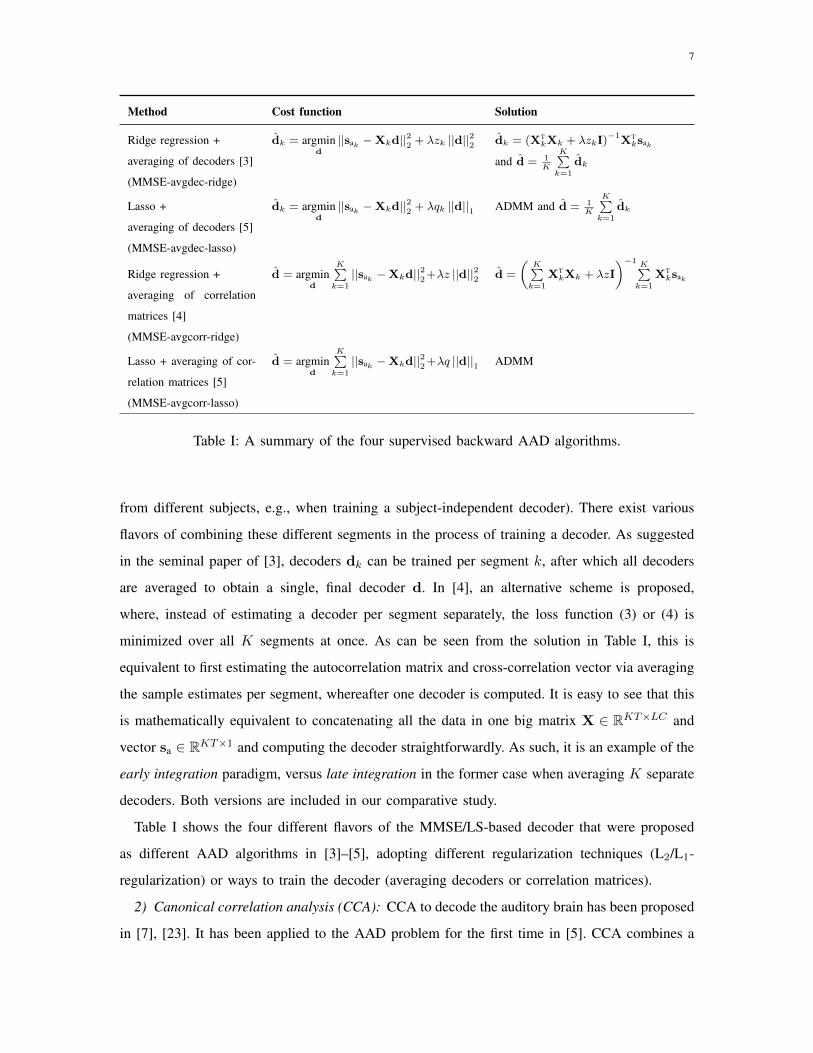
Method Cost function Solution

Ridge regression +

averaging of decoders [3]

(MMSE-avgdec-ridge)

dk = argmind

||sak −Xkd||22 + λzk ||d||22 dk = (XTkXk + λzkI)

−1XT

ksak

and d = 1K

K∑k=1

dk

Lasso +

averaging of decoders [5]

(MMSE-avgdec-lasso)

dk = argmind

||sak −Xkd||22 + λqk ||d||1 ADMM and d = 1K

K∑k=1

dk

Ridge regression +

averaging of correlation

matrices [4]

(MMSE-avgcorr-ridge)

d = argmind

K∑k=1

||sak −Xkd||22+λz ||d||22 d =

(K∑

k=1

XTkXk + λzI

)−1 K∑k=1

XTksak

Lasso + averaging of cor-

relation matrices [5]

(MMSE-avgcorr-lasso)

d = argmind

K∑k=1

||sak −Xkd||22+λq ||d||1 ADMM

Table I: A summary of the four supervised backward AAD algorithms.

from different subjects, e.g., when training a subject-independent decoder). There exist various

flavors of combining these different segments in the process of training a decoder. As suggested

in the seminal paper of [3], decoders dk can be trained per segment k, after which all decoders

are averaged to obtain a single, final decoder d. In [4], an alternative scheme is proposed,

where, instead of estimating a decoder per segment separately, the loss function (3) or (4) is

minimized over all K segments at once. As can be seen from the solution in Table I, this is

equivalent to first estimating the autocorrelation matrix and cross-correlation vector via averaging

the sample estimates per segment, whereafter one decoder is computed. It is easy to see that this

is mathematically equivalent to concatenating all the data in one big matrix X ∈ RKT×LC and

vector sa ∈ RKT×1 and computing the decoder straightforwardly. As such, it is an example of the

early integration paradigm, versus late integration in the former case when averaging K separate

decoders. Both versions are included in our comparative study.

Table I shows the four different flavors of the MMSE/LS-based decoder that were proposed

as different AAD algorithms in [3]–[5], adopting different regularization techniques (L2/L1-

regularization) or ways to train the decoder (averaging decoders or correlation matrices).

2) Canonical correlation analysis (CCA): CCA to decode the auditory brain has been proposed

in [7], [23]. It has been applied to the AAD problem for the first time in [5]. CCA combines a

8

spatio-temporal backward (decoding) model wx ∈ RLC×1 on the EEG and a temporal forward

(encoding) model wsa ∈ RLa×1 on the speech envelope, with La the number of filter taps of the

encoding filter. In this sense, CCA differs from the previous approaches, which were all different

flavors of the same MMSE/LS-based decoder. In CCA, both the forward and backward model

are estimated jointly such that their outputs are maximally correlated:

maxwx,wsa

E{(wT

xx(t))(wT

sasa(t)

)}√E{(wT

xx(t))2}√

E{(

wTsasa(t)

)2} = maxwx,wsa

wTxRxsawsa√

wTxRxxwx

√wT

saRsasawsa

, (5)

where sa(t) =[sa(t) sa(t− 1) · · · sa(t− La + 1)

]T

∈ RLa×1. Note that the audio filter wsa

is a causal filter (as opposed to the EEG filter wx), as the stimulus precedes the brain response.

The solution of the optimization problem in (5) can be easily retrieved by solving a generalized

eigenvalue decomposition (details in [4], [5]).

In CCA, the backward model wx and forward model wsa are extended to a set of J filters

Wx ∈ RLC×J and Wsa ∈ RLa×J for which the outputs are maximally correlated, but mutually

uncorrelated (the J outputs of WTxx(t) are uncorrelated to each other and the J outputs of

WTsasa(t) are uncorrelated to each other). There are now thus J Pearson correlation coefficients

between the outputs of the J backward and forward filters (aka canonical correlation coefficients),

which are collected in the vector ρi ∈ RJ×1 for speaker i, whereas before, there was only one

per speaker. Furthermore, because of the way CCA constructs the filters, it can be expected

that the first components are more important than the later ones. To find the optimal way of

combining the canonical correlation coefficients, a linear discriminant analysis (LDA) classifier

can be trained, as proposed in [7]. To generalize the maximization of the correlation coefficients

of the previous AAD algorithms (which is equivalent to taking the sign of the difference of

the correlation coefficients of both speakers), we propose here to construct a feature vector

f ∈ RJ×1 by subtracting the canonical correlation vectors: f = ρ1 − ρ2, and classify f with an

LDA classifier. As proposed in [7], PCA is being used as a preprocessing step on the EEG, to

reduce the number of parameters. In fact, this is a way of regularizing CCA and can as such be

viewed as an alternative to the regularization techniques proposed in other methods.

3) Training-free MMSE-based with lasso (MMSE-adap-lasso): In [6], a fundamentally dif-

ferent AAD algorithm is proposed. All other AAD algorithms in this comparative study are

supervised, batch-trained algorithms, which have a separate training and testing stage. First, the

decoders need to be trained in a supervised manner using a large amount of ground-truth data,

after which they can be applied to new test data. In practice, this necessitates a (potentially

9

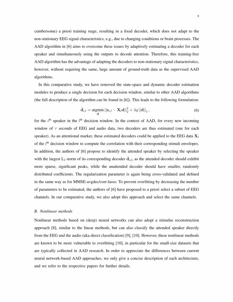
cumbersome) a priori training stage, resulting in a fixed decoder, which does not adapt to the

non-stationary EEG signal characteristics, e.g., due to changing conditions or brain processes. The

AAD algorithm in [6] aims to overcome these issues by adaptively estimating a decoder for each

speaker and simultaneously using the outputs to decode attention. Therefore, this training-free

AAD algorithm has the advantage of adapting the decoders to non-stationary signal characteristics,

however, without requiring the same, large amount of ground-truth data as the supervised AAD

algorithms.

In this comparative study, we have removed the state-space and dynamic decoder estimation

modules to produce a single decision for each decision window, similar to other AAD algorithms

(the full description of the algorithm can be found in [6]). This leads to the following formulation:

di,l = argmind||si,l −Xld||22 + λq ||d||1 , (6)

for the ith speaker in the lth decision window. In the context of AAD, for every new incoming

window of τ seconds of EEG and audio data, two decoders are thus estimated (one for each

speaker). As an attentional marker, these estimated decoders could be applied to the EEG data Xl

of the lth decision window to compute the correlation with their corresponding stimuli envelopes.

In addition, the authors of [6] propose to identify the attended speaker by selecting the speaker

with the largest L1-norm of its corresponding decoder di,l, as the attended decoder should exhibit

more sparse, significant peaks, while the unattended decoder should have smaller, randomly

distributed coefficients. The regularization parameter is again being cross-validated and defined

in the same way as for MMSE-avgdec/corr-lasso. To prevent overfitting by decreasing the number

of parameters to be estimated, the authors of [6] have proposed to a priori select a subset of EEG

channels. In our comparative study, we also adopt this approach and select the same channels.

B. Nonlinear methods

Nonlinear methods based on (deep) neural networks can also adopt a stimulus reconstruction

approach [8], similar to the linear methods, but can also classify the attended speaker directly

from the EEG and the audio (aka direct classification) [9], [10]. However, these nonlinear methods

are known to be more vulnerable to overfitting [10], in particular for the small-size datasets that

are typically collected in AAD research. In order to appreciate the differences between current

neural network-based AAD approaches, we only give a concise description of each architecture,

and we refer to the respective papers for further details.

10

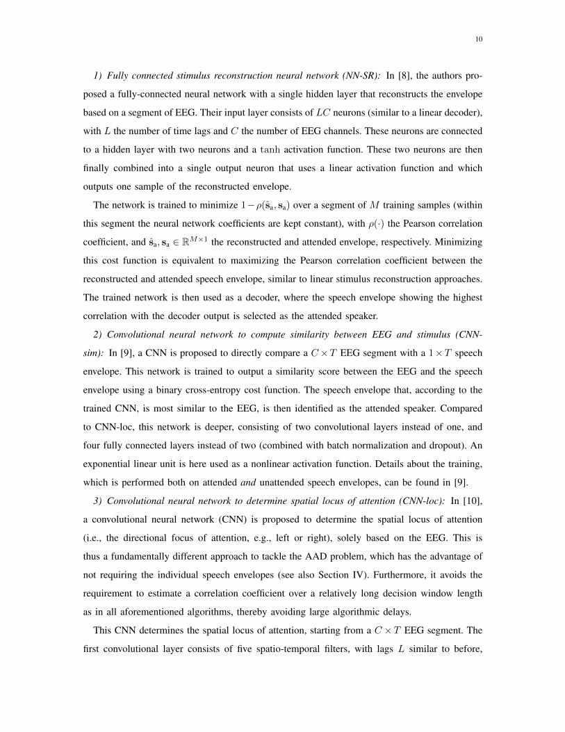
1) Fully connected stimulus reconstruction neural network (NN-SR): In [8], the authors pro-

posed a fully-connected neural network with a single hidden layer that reconstructs the envelope

based on a segment of EEG. Their input layer consists of LC neurons (similar to a linear decoder),

with L the number of time lags and C the number of EEG channels. These neurons are connected

to a hidden layer with two neurons and a tanh activation function. These two neurons are then

finally combined into a single output neuron that uses a linear activation function and which

outputs one sample of the reconstructed envelope.

The network is trained to minimize 1−ρ(sa, sa) over a segment of M training samples (within

this segment the neural network coefficients are kept constant), with ρ(·) the Pearson correlation

coefficient, and sa, sa ∈ RM×1 the reconstructed and attended envelope, respectively. Minimizing

this cost function is equivalent to maximizing the Pearson correlation coefficient between the

reconstructed and attended speech envelope, similar to linear stimulus reconstruction approaches.

The trained network is then used as a decoder, where the speech envelope showing the highest

correlation with the decoder output is selected as the attended speaker.

2) Convolutional neural network to compute similarity between EEG and stimulus (CNN-

sim): In [9], a CNN is proposed to directly compare a C×T EEG segment with a 1×T speech

envelope. This network is trained to output a similarity score between the EEG and the speech

envelope using a binary cross-entropy cost function. The speech envelope that, according to the

trained CNN, is most similar to the EEG, is then identified as the attended speaker. Compared

to CNN-loc, this network is deeper, consisting of two convolutional layers instead of one, and

four fully connected layers instead of two (combined with batch normalization and dropout). An

exponential linear unit is here used as a nonlinear activation function. Details about the training,

which is performed both on attended and unattended speech envelopes, can be found in [9].

3) Convolutional neural network to determine spatial locus of attention (CNN-loc): In [10],

a convolutional neural network (CNN) is proposed to determine the spatial locus of attention

(i.e., the directional focus of attention, e.g., left or right), solely based on the EEG. This is

thus a fundamentally different approach to tackle the AAD problem, which has the advantage of

not requiring the individual speech envelopes (see also Section IV). Furthermore, it avoids the

requirement to estimate a correlation coefficient over a relatively long decision window length

as in all aforementioned algorithms, thereby avoiding large algorithmic delays.

This CNN determines the spatial locus of attention, starting from a C ×T EEG segment. The

first convolutional layer consists of five spatio-temporal filters, with lags L similar to before,

11

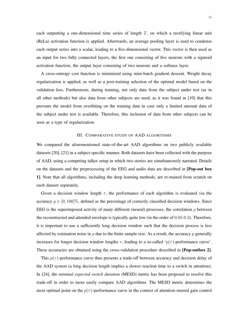
each outputting a one-dimensional time series of length T , on which a rectifying linear unit

(ReLu) activation function is applied. Afterwards, an average pooling layer is used to condense

each output series into a scalar, leading to a five-dimensional vector. This vector is then used as

an input for two fully connected layers, the first one consisting of five neurons with a sigmoid

activation function, the output layer consisting of two neurons and a softmax layer.

A cross-entropy cost function is minimized using mini-batch gradient descent. Weight decay

regularization is applied, as well as a post-training selection of the optimal model based on the

validation loss. Furthermore, during training, not only data from the subject under test (as in

all other methods) but also data from other subjects are used, as it was found in [10] that this

prevents the model from overfitting on the training data in case only a limited amount data of

the subject under test is available. Therefore, this inclusion of data from other subjects can be

seen as a type of regularization.

III. COMPARATIVE STUDY OF AAD ALGORITHMS

We compared the aforementioned state-of-the-art AAD algorithms on two publicly available

datasets [20], [21] in a subject-specific manner. Both datasets have been collected with the purpose

of AAD, using a competing talker setup in which two stories are simultaneously narrated. Details

on the datasets and the preprocessing of the EEG and audio data are described in [Pop-out box

1]. Note that all algorithms, including the deep learning methods, are re-trained from scratch on

each dataset separately.

Given a decision window length τ , the performance of each algorithm is evaluated via the

accuracy p ∈ [0, 100]%, defined as the percentage of correctly classified decision windows. Since

EEG is the superimposed activity of many different (neural) processes, the correlation ρ between

the reconstructed and attended envelope is typically quite low (in the order of 0.05-0.2). Therefore,

it is important to use a sufficiently long decision window such that the decision process is less

affected by estimation noise in ρ due to the finite sample size. As a result, the accuracy p generally

increases for longer decision window lengths τ , leading to a so-called ‘p(τ)-performance curve’.

These accuracies are obtained using the cross-validation procedure described in [Pop-outbox 2].

This p(τ)-performance curve thus presents a trade-off between accuracy and decision delay of

the AAD system (a long decision length implies a slower reaction time to a switch in attention).

In [24], the minimal expected switch duration (MESD) metric has been proposed to resolve this

trade-off in order to more easily compare AAD algorithms. The MESD metric determines the

most optimal point on the p(τ)-performance curve in the context of attention-steered gain control

12

by minimizing the expected time it takes to switch the gain between two speakers in an optimized

robust gain control system. As such, it outputs a single-number time metric (the MESD [s]) for a

p(τ)-performance curve and thus removes the loss of statistical power due to multiple-comparison

corrections in statistical hypothesis testing (due to testing for multiple decision window lengths).

Furthermore, the MESD ensures that the statistical comparison is automatically focused on the

most practically relevant points on the p(τ)-performance curve, which typically turn out to be the

ones corresponding to short decision window lengths τ < 10 s [24]. Note that a higher MESD

corresponds to a worse AAD performance and vice versa.

A. Statistical analysis

To statistically compare the included AAD algorithms, we adopt a linear mixed-effects model

(LMM) on the MESD values with the AAD algorithm as a fixed effect and with subjects as

a repeated-measure random effect. Five contrasts of interest were set a priori according to the

binary tree structure in Fig. 3. Algorithms that did not perform significantly better than chance

are excluded from the statistical analysis, which is why some algorithms are not included in the

contrasts (see Section III-B1). The planned contrasts reflect the most important different features

between AAD algorithms, as shown in Fig. 3, motivating the way they are set. The significance

level is set at α = 0.05.

B. Results

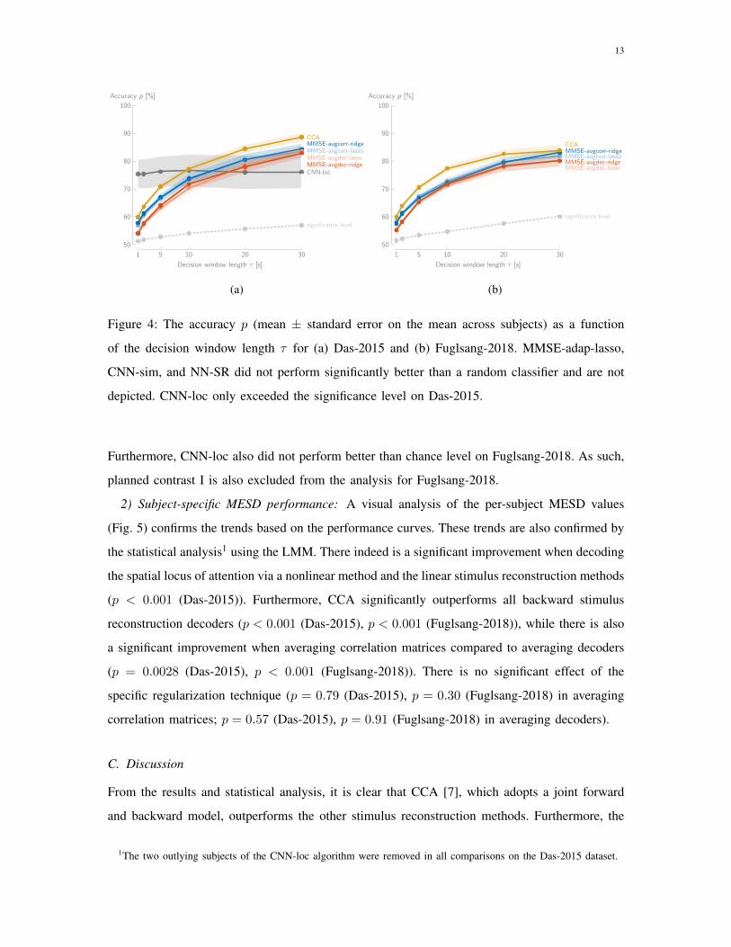
1) Performance curves: Fig. 4 shows the p(τ)-performance curves of the different AAD

algorithms on both datasets. For the MMSE-based decoders, it is observed that there barely is

an effect of the type of regularization, and that averaging correlation matrices (early integration)

consistently outperforms averaging decoders (late integration). Furthermore, CCA outperforms

all other linear algorithms. Lastly, on Das-2015, it is clear that decoding the spatial locus of

attention using CNN-loc substantially outperforms the stimulus reconstruction methods for short

decision windows (< 10 s), where CNN-loc appears to be less affected by the decision window

length. However, the standard error on the mean is much higher for the CNN-loc algorithm than

for the other methods, indicating a higher inter-subject variability.

The performances of MMSE-adap-lasso, CNN-sim, and NN-SR are not shown in Fig. 4 as

they did not exceed the significance level on either of the two datasets. As these algorithms did

not significantly outperform a random classifier, they were excluded from the statistical analysis.

13

1 5 10 20 3050

60

70

80

90

100

significance level

CNN-loc

MMSE-avgcorr-lassoMMSE-avgcorr-ridge

MMSE-avgdec-lassoMMSE-avgdec-ridge

CCA

Decision window length τ [s]

Accuracy p [%]

(a)

1 5 10 20 3050

60

70

80

90

100

significance level

MMSE-avgcorr-lassoMMSE-avgcorr-ridge

MMSE-avgdec-lassoMMSE-avgdec-ridge

CCA

Decision window length τ [s]

Accuracy p [%]

(b)

Figure 4: The accuracy p (mean ± standard error on the mean across subjects) as a function

of the decision window length τ for (a) Das-2015 and (b) Fuglsang-2018. MMSE-adap-lasso,

CNN-sim, and NN-SR did not perform significantly better than a random classifier and are not

depicted. CNN-loc only exceeded the significance level on Das-2015.

Furthermore, CNN-loc also did not perform better than chance level on Fuglsang-2018. As such,

planned contrast I is also excluded from the analysis for Fuglsang-2018.

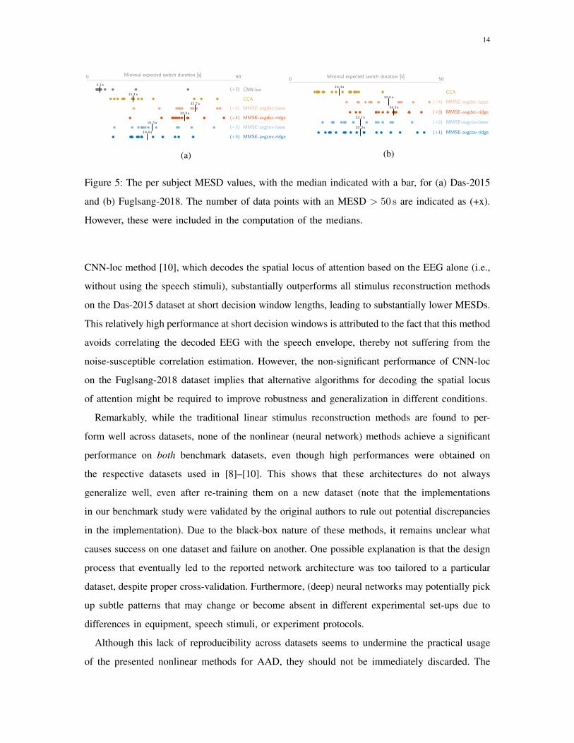
2) Subject-specific MESD performance: A visual analysis of the per-subject MESD values

(Fig. 5) confirms the trends based on the performance curves. These trends are also confirmed by

the statistical analysis1 using the LMM. There indeed is a significant improvement when decoding

the spatial locus of attention via a nonlinear method and the linear stimulus reconstruction methods

(p < 0.001 (Das-2015)). Furthermore, CCA significantly outperforms all backward stimulus

reconstruction decoders (p < 0.001 (Das-2015), p < 0.001 (Fuglsang-2018)), while there is also

a significant improvement when averaging correlation matrices compared to averaging decoders

(p = 0.0028 (Das-2015), p < 0.001 (Fuglsang-2018)). There is no significant effect of the

specific regularization technique (p = 0.79 (Das-2015), p = 0.30 (Fuglsang-2018) in averaging

correlation matrices; p = 0.57 (Das-2015), p = 0.91 (Fuglsang-2018) in averaging decoders).

C. Discussion

From the results and statistical analysis, it is clear that CCA [7], which adopts a joint forward

and backward model, outperforms the other stimulus reconstruction methods. Furthermore, the

1The two outlying subjects of the CNN-loc algorithm were removed in all comparisons on the Das-2015 dataset.

14

0 50

19.8 sMMSE-avgcov-ridge(+3)

32.2 sMMSE-avgdec-ridge(+4)

35.7 sMMSE-avgdec-lasso(+5)

21.5 sMMSE-avgcov-lasso(+3)

15.1 sCCA

4.1 sCNN-loc(+2)

Minimal expected switch duration [s]

(a)

0 50

23.2 sMMSE-avgcov-ridge(+1)

34.3 sMMSE-avgdec-ridge(+3)

23.1 sMMSE-avgcov-lasso(+2)

32.6 sMMSE-avgdec-lasso(+4)

16.3 sCCA

Minimal expected switch duration [s]

(b)

Figure 5: The per subject MESD values, with the median indicated with a bar, for (a) Das-2015

and (b) Fuglsang-2018. The number of data points with an MESD > 50 s are indicated as (+x).

However, these were included in the computation of the medians.

CNN-loc method [10], which decodes the spatial locus of attention based on the EEG alone (i.e.,

without using the speech stimuli), substantially outperforms all stimulus reconstruction methods

on the Das-2015 dataset at short decision window lengths, leading to substantially lower MESDs.

This relatively high performance at short decision windows is attributed to the fact that this method

avoids correlating the decoded EEG with the speech envelope, thereby not suffering from the

noise-susceptible correlation estimation. However, the non-significant performance of CNN-loc

on the Fuglsang-2018 dataset implies that alternative algorithms for decoding the spatial locus

of attention might be required to improve robustness and generalization in different conditions.

Remarkably, while the traditional linear stimulus reconstruction methods are found to per-

form well across datasets, none of the nonlinear (neural network) methods achieve a significant

performance on both benchmark datasets, even though high performances were obtained on

the respective datasets used in [8]–[10]. This shows that these architectures do not always

generalize well, even after re-training them on a new dataset (note that the implementations

in our benchmark study were validated by the original authors to rule out potential discrepancies

in the implementation). Due to the black-box nature of these methods, it remains unclear what

causes success on one dataset and failure on another. One possible explanation is that the design

process that eventually led to the reported network architecture was too tailored to a particular

dataset, despite proper cross-validation. Furthermore, (deep) neural networks may potentially pick

up subtle patterns that may change or become absent in different experimental set-ups due to

differences in equipment, speech stimuli, or experiment protocols.

Although this lack of reproducibility across datasets seems to undermine the practical usage

of the presented nonlinear methods for AAD, they should not be immediately discarded. The

15

current benchmark datasets are possibly too small for these methods to draw firm conclusions.

AAD based on (deep) neural networks may become more robust when larger datasets become

available, containing more subjects, more EEG data per subject, and more variation in experimen-

tal conditions. Nevertheless, the results of this comparative study point out the risks of overfitting

and overdesigning these architectures, thereby emphasizing the importance of extensive validation

with multiple datasets.

IV. OPEN CHALLENGES AND OUTLOOK

A. Effects of speaker separation and denoising algorithms

As explained in Section II, most AAD algorithms require access to the speech envelopes of the

individual speakers. However, in the context of neuro-steered hearing devices, this would require

the extraction of these per-speaker envelopes from the hearing aid’s microphone recordings. It is

expected that the performed speaker separation is not perfect, affecting the quality of the speech

envelopes, and thus also affecting the AAD algorithms that use these envelopes. Correspondingly,

AAD algorithms that do not rely on this speaker separation step, such as decoding the spatial locus

of attention [10], have an inherent major advantage. In any case, a speech enhancement algorithm

is required to eventually extract the attended speaker, for which advanced and well-performing

signal processing algorithms exist (e.g., [25]–[27]).

A few studies have already combined AAD with speaker separation and denoising algorithms,

both using traditional beamforming approaches [11], [15], [28], and deep neural networks for

speaker separation [12], [13], [28]. Remarkably, many of these studies show only minor or hardly

any effects on the AAD performance when using the demixed speech signals, even in challenging

noisy conditions [15], [28], and despite significant distortions on the envelopes. These positive

results are paramount for the practical applicability of neuro-steered hearing devices.

Finally, instead of treating the speaker extraction and AAD as two separate problems (as is the

case in all aforementioned studies), one could also aim to solve both problems simultaneously.

In [14], the speaker extraction and AAD problem are coupled together in a joint optimization

problem, where the beamformer is enforced to generate an output signal that is correlated to the

output of a backward MMSE neural decoder.

B. EEG miniaturization and wearability effects

The data used in this paper are recorded using expensive, heavy, and bulky EEG recording

systems. The realization of neuro-steered hearing devices requires a wearable, concealable EEG

16

monitoring system. The research towards such concealable EEG systems is very active, resulting

in novel devices that acquire the EEG for example in the ear (e.g., [17]) or around the ear

(e.g., [16]). Such wearable, concealable EEG systems, however, provide only a limited amount

of EEG channels, which only record brain activity within a small area. A first analysis using such

an around-the-ear EEG system in the context of AAD showed potential, albeit with a significant

decrease in performance [18].

In another (top-down) approach, the optimal number and location of miniaturized EEG sensors

(combined in nodes) are determined in the context of AAD [19]. It was shown that using a data-

driven selection of the best 10 EEG channels of a standard 64-channel EEG cap does not reduce

the AAD performance. Moreover, in the same work, it was also demonstrated that using EEG

measured by mini-EEG devices with electrodes separated by short distances, results in similar

performances to EEG measured using long-distance EEG montages, when these mini-EEG devices

are positioned strategically on the scalp.

C. Outlook

Several studies have demonstrated that it is possible to decode the auditory attention from a non-

invasive neurorecording technique such as EEG. In our comparative study, we have shown that

most of these results are reproducible on different data sets. However, even for the best linear

(stimulus reconstruction) method (CCA), the accuracy at short decision windows is still too low,

potentially leading to too slow reactions of the system to shifts in auditory attention, as indicated

by a median MESD of 15 s. The results of this study have demonstrated that an alternative

strategy, such as decoding the spatial locus of attention, could significantly improve on these

short decision window lengths. Although nonlinear (deep learning) methods are believed to be

able to substantially improve AAD performances, our study has demonstrated that the reported

results obtained by these methods are hard to replicate on multiple independent AAD datasets. A

major future challenge for AAD research is the design of an algorithm or strategy that reliably

improves on short decision windows, and which is reproducible on different independent datasets.

Furthermore, most of the presented AAD algorithms require supervised training and are fixed

during operation. To avoid cumbersome a priori training sessions for each individual user, as

well as to adapt to the time-varying statistics of the EEG (e.g., in different listening scenarios),

training-free or unsupervised adaptive AAD algorithms should be developed. While several steps

have been made in that direction [6], the results of this study show that we are still far away

from a practical solution.

17

Furthermore, these AAD algorithms need to be further evaluated in real-life situations, taking

various realistic listening scenarios into account, as well as on potential hearing device users [29].

The individual building blocks of a neuro-steered hearing device (Fig. 1) need to be integrated,

in which an AAD algorithm is combined with a reliable and low-latency speaker separation

algorithm, a miniaturized EEG sensor system, and a smart gain control system.

Despite the many challenges ahead, the application of neuro-steered hearing devices as a neu-

rorehabilitative assistive device has shown to be within reach, having the potential to substantially

improve the functionality and user-acceptance of future generations of hearing devices.

POP-OUT BOXES

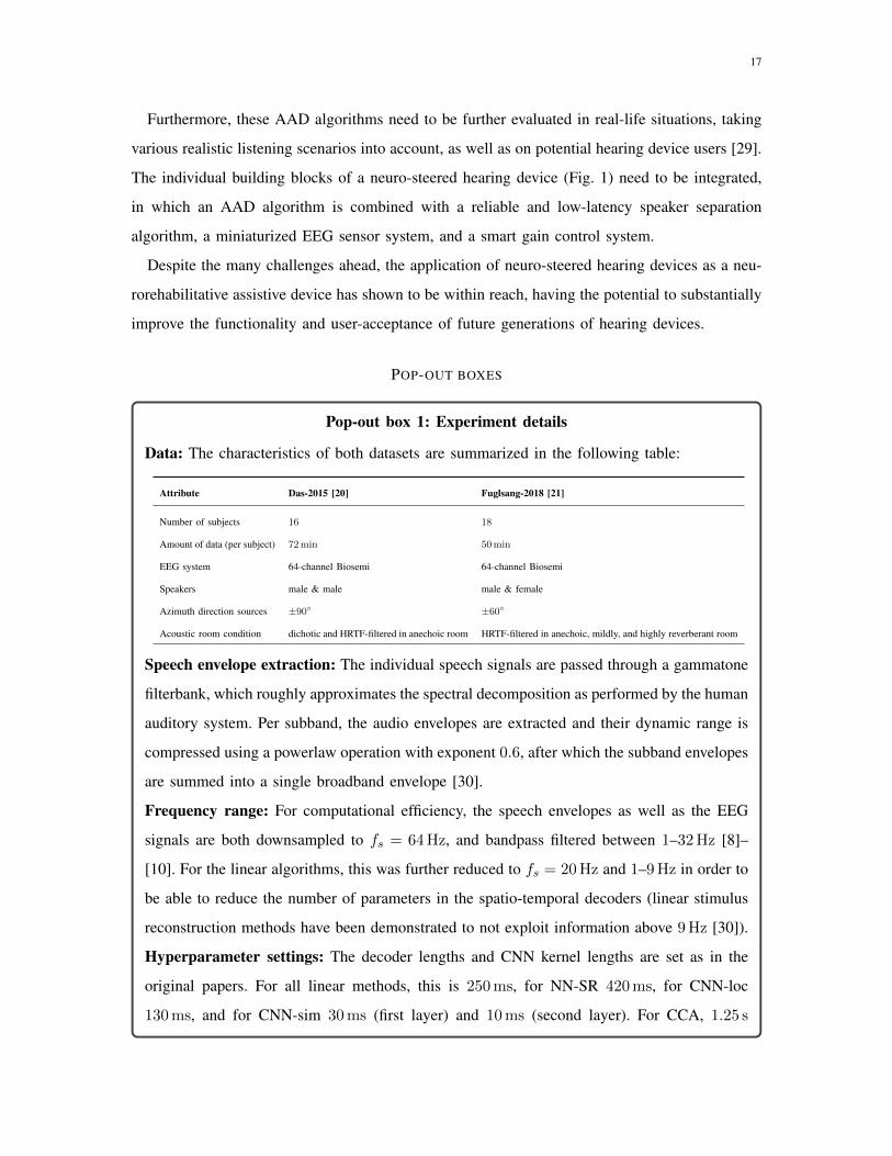
Pop-out box 1: Experiment details

Data: The characteristics of both datasets are summarized in the following table:

Attribute Das-2015 [20] Fuglsang-2018 [21]

Number of subjects 16 18

Amount of data (per subject) 72min 50min

EEG system 64-channel Biosemi 64-channel Biosemi

Speakers male & male male & female

Azimuth direction sources ±90◦ ±60◦

Acoustic room condition dichotic and HRTF-filtered in anechoic room HRTF-filtered in anechoic, mildly, and highly reverberant room

Speech envelope extraction: The individual speech signals are passed through a gammatone

filterbank, which roughly approximates the spectral decomposition as performed by the human

auditory system. Per subband, the audio envelopes are extracted and their dynamic range is

compressed using a powerlaw operation with exponent 0.6, after which the subband envelopes

are summed into a single broadband envelope [30].

Frequency range: For computational efficiency, the speech envelopes as well as the EEG

signals are both downsampled to fs = 64Hz, and bandpass filtered between 1–32Hz [8]–

[10]. For the linear algorithms, this was further reduced to fs = 20Hz and 1–9Hz in order to

be able to reduce the number of parameters in the spatio-temporal decoders (linear stimulus

reconstruction methods have been demonstrated to not exploit information above 9Hz [30]).

Hyperparameter settings: The decoder lengths and CNN kernel lengths are set as in the

original papers. For all linear methods, this is 250ms, for NN-SR 420ms, for CNN-loc

130ms, and for CNN-sim 30ms (first layer) and 10ms (second layer). For CCA, 1.25 s

18

is chosen as the encoder length. The full set of 64 channels are used in all algorithms,

except for MMSE-adap-lasso, where the same 28 channels as in [6] are chosen to reduce the

number of parameters (since the decoder is estimated on much less data). The regularization

parameters are cross-validated using 10 values in the range [10−6, 0]. For CCA, it turned out

that retaining all PCA components for both datasets is optimal.

Pop-out box 2: Details on cross-validation procedure

Two-stage cross-validation: The different algorithms are evaluated via a two-stage cross-

validation (CV) procedure applied per subject and decision window length. The AAD accuracy

is determined via an outer leave-one-segment-out CV (LOSO-CV) loop. Per outer fold, the

optimal hyperparameter is determined via an inner ten-fold CV loop on the training set of

the outer loop. The length of each left-out segment in the outer loop is chosen equal to 60 s,

which is split into smaller disjoint decision windows. For example, for a decision window

length of 30 s, each left-out segment results in two decisions. Additional details per AAD

algorithm are provided in the following table (standard CV corresponds to training on all but

one segment, testing on the left-out segment):

Method Outer LOSO-CV loop Inner 10-CV loop

MMSE-avgcorr-

ridge/lasso

standard optimization of λ (independent of τ , tuned based on

largest value of τ )

MMSE-avgdec-

ridge/lasso

training data of each fold is split into windows of the

same size as τ . A different decoder is estimated in each of

these subwindows and the decoders are averaged across

all training folds (similar to [3])

optimization of λ (re-optimized for τ due to the depen-

dency of the training procedure on τ )

CCA standard, additional LOSO-CV loop to train and test LDA

classifier

optimization of the number of canonical correlation co-

efficients J as input for LDA (re-optimized for each τ )

MMSE-adap-lasso optimization of λ per τ and fold by taking hyperparam-

eter with highest accuracy on training fold

/

NN-SR standard /

CNN-loc LOSpO-CV instead of LOSO-CV, training and testing

redone for τ

/

CNN-sim standard, training and testing redone for τ /

Overfitting to speakers: The CNN-loc algorithm has been shown to be prone to overfitting

to speakers in the training set, thus showing overoptimistic performance when using the

LOSO-CV method, where the test set always contains a speaker that is also present in the

19

training set [10]. Instead, we use the leave-one-speaker-out CV (LOSpO-CV) method for this

algorithm, as explained in [10]. For the linear methods we use the standard LOSO-CV as these

do not exhibit such overfitting. The latter is validated by performing 100 runs per subject, with

in each run another random CV split (using the same amount of folds as for LOSpO-CV).

We then tested whether the LOSpO-CV performance significantly differs from the median

of this empirical distribution (i.e., the median over all random splits) over all subjects. For

the CCA method, which has most degrees of freedom to overfit, the difference between the

LOSpO-CV and median random-CV accuracy is less than 1% on 20s decision windows, and

a paired Wilcoxon signed-rank test (over subjects) shows no significant difference (W =

85, n = 16, p = 0.38), indicating that there is no significant overfitting effect.

REFERENCES

[1] N. Mesgarani and E. F. Chang, “Selective cortical representation of attended speaker in multi-talker speech

perception,” Nature, vol. 485, no. 7397, pp. 233–236, 2012.

[2] N. Ding and J. Z. Simon, “Emergence of neural encoding of auditory objects while listening to competing

speakers,” Proc. Natl. Acad. Sci., vol. 109, no. 29, pp. 11 854–11 859, 2012.

[3] J. A. O’Sullivan et al., “Attentional Selection in a Cocktail Party Environment Can Be Decoded from Single-Trial

EEG,” Cereb. Cortex, vol. 25, no. 7, pp. 1697–1706, 2014.

[4] W. Biesmans et al., “Auditory-inspired speech envelope extraction methods for improved EEG-based auditory

attention detection in a cocktail party scenario,” IEEE Trans. Neural Syst. Rehabil. Eng., vol. 25, no. 5, pp.

402–412, 2017.

[5] E. Alickovic et al., “A Tutorial on Auditory Attention Identification Methods,” Front. Neurosci., vol. 13, p. 153,

2019.

[6] S. Miran et al., “Real-Time Tracking of Selective Auditory Attention from M/EEG: A Bayesian Filtering

Approach,” Front. Neurosci., vol. 12, p. 262, 2018.

[7] A. de Cheveigne et al., “Decoding the auditory brain with canonical component analysis,” NeuroImage, vol. 172,

pp. 206–216, 2018.

[8] T. de Taillez et al., “Machine learning for decoding listeners attention from electroencephalography evoked by

continuous speech,” Eur. J. Neurosci., 2017.

[9] G. Ciccarelli et al., “Comparison of Two-Talker Attention Decoding from EEG with Nonlinear Neural Networks

and Linear Methods,” Sci Rep, vol. 9, no. 1, p. 11538, 2019.

[10] S. Vandecappelle et al., “EEG-based detection of the locus of auditory attention with convolutional neural

networks,” bioRxiv, 2020. [Online]. Available: https://www.biorxiv.org/content/early/2020/02/27/475673

[11] S. Van Eyndhoven et al., “EEG-Informed Attended Speaker Extraction From Recorded Speech Mixtures With

Application in Neuro-Steered Hearing Prostheses,” IEEE Trans. Biomed. Eng., vol. 64, no. 5, pp. 1045–1056,

2017.

20

[12] J. OSullivan et al., “Neural decoding of attentional selection in multi-speaker environments without access to

clean sources,” J. Neural Eng., vol. 14, no. 5, p. 056001, 2017.

[13] C. Han et al., “Speaker-independent auditory attention decoding without access to clean speech sources,” Sci.

Adv., vol. 5, no. 5, pp. 1–12, 2019.

[14] W. Pu et al., “A Joint Auditory Attention Decoding and Adaptive Binaural Beamforming Algorithm for Hearing

Devices,” in Proc. IEEE Int. Conf. Acoust. Speech and Signal Process., 2019, pp. 311–315.

[15] A. Aroudi and S. Doclo, “Cognitive-driven binaural beamforming using EEG-based auditory attention decoding,”

IEEE/ACM Trans. Audio, Speech, Language Process., vol. 28, pp. 862–875, 2020.

[16] S. Debener et al., “Unobtrusive ambulatory EEG using a smartphone and flexible printed electrodes around the

ear,” Sci Rep, vol. 5, p. 16743, 2015.

[17] S. L. Kappel et al., “Dry-Contact Electrode Ear-EEG,” IEEE Trans. Biomed. Eng., vol. 66, no. 1, pp. 150–158,

2019.

[18] B. Mirkovic et al., “Target Speaker Detection with Concealed EEG Around the Ear,” Front. Neurosci., vol. 10,

p. 349, 2016.

[19] A. M. Narayanan and A. Bertrand, “Analysis of miniaturization effects and channel selection strategies for EEG

sensor networks with application to auditory attention detection,” IEEE Trans. Biomed. Eng., vol. 67, no. 1, pp.

234–244, 2020.

[20] N. Das et al., “Auditory Attention Detection Dataset KULeuven,” Zenodo, 2019. [Online]. Available:

https://doi.org/10.5281/zenodo.3377911

[21] S. A. Fuglsang et al., “EEG and audio dataset for auditory attention decoding,” Zenodo, 2018. [Online].

Available: https://doi.org/10.5281/zenodo.1199011

[22] D. D. E. Wong et al., “A Comparison of Regularization Methods in Forward and Backward Models for Auditory

Attention Decoding,” Front. Neurosci., vol. 12, p. 531, 2018.

[23] J. P. Dmochowski et al., “Extracting multidimensional stimulus-response correlations using hybrid encoding-

decoding of neural activity,” NeuroImage, vol. 180, pp. 134–146, 2018.

[24] S. Geirnaert et al., “An Interpretable Performance Metric for Auditory Attention Decoding Algorithms in a

Context of Neuro-Steered Gain Control,” IEEE Trans. Neural Syst. Rehabil. Eng., vol. 28, no. 1, pp. 307–317,

2020.

[25] T. Gerkmann et al., “Phase processing for single-channel speech enhancement: History and recent advances,”

IEEE Signal Process. Mag., vol. 32, no. 2, pp. 55–66, 2015.

[26] S. Gannot et al., “A Consolidated Perspective on Multimicrophone Speech Enhancement and Source Separation,”

IEEE/ACM Trans. Audio, Speech, Language Process., vol. 25, no. 4, pp. 692–730, 2017.

[27] Y. Luo and N. Mesgarani, “Conv-TasNet: Surpassing Ideal Time-Frequency Magnitude Masking for Speech

Separation,” IEEE/ACM Trans. Audio, Speech, Language Process., vol. 27, no. 8, pp. 1256–1266, 2019.

[28] N. Das et al., “Linear versus deep learning methods for noisy speech separation for EEG-informed attention

decoding,” J. Neural Eng., 2020.

[29] S. A. Fuglsang et al., “Effects of Sensorineural Hearing Loss on Cortical Synchronization to Competing Speech

during Selective Attention,” J. Neurosci., vol. 40, no. 12, pp. 2562–2572, 2020.

[30] N. Das et al., “The effect of head-related filtering and ear-specific decoding bias on auditory attention detection,”

J. Neural Eng., vol. 13, no. 5, p. 056014, 2016.