Embed Size (px)
Citation preview

Neural Systems for Control1
Omid M. Omidvar and David L. Elliott, Editors
February, 1997
1This the complete book (but with different pagination) Neural Systemsfor Control, O. M. Omidvar and D. L. Elliott, editors, Copyright 1997 byAcademic Press, ISBN: 0125264305 and is posted with permission from Elsevier.http://www.isr.umd.edu/∼delliott/NeuralSystemsForControl.pdf

ii

Contents
Contributors vii
Preface xi
1 Introduction: Neural Networks and Automatic Control 11 Control Systems . . . . . . . . . . . . . . . . . . . . . . . . 12 What is a Neural Network? . . . . . . . . . . . . . . . . . . 3
2 Reinforcement Learning 71 Introduction . . . . . . . . . . . . . . . . . . . . . . . . . . . 72 Non-Associative Reinforcement Learning . . . . . . . . . . . 83 Associative Reinforcement Learning . . . . . . . . . . . . . 124 Sequential Reinforcement Learning . . . . . . . . . . . . . . 205 Conclusion . . . . . . . . . . . . . . . . . . . . . . . . . . . 266 References . . . . . . . . . . . . . . . . . . . . . . . . . . . . 27
3 Neurocontrol in Sequence Recognition 311 Introduction . . . . . . . . . . . . . . . . . . . . . . . . . . . 312 HMM Source Models . . . . . . . . . . . . . . . . . . . . . . 323 Recognition: Finding the Best Hidden Sequence . . . . . . . 334 Controlled Sequence Recognition . . . . . . . . . . . . . . . 345 A Sequential Event Dynamic Neural Network . . . . . . . . 426 Neurocontrol in sequence recognition . . . . . . . . . . . . . 497 Observations and Speculations . . . . . . . . . . . . . . . . 528 References . . . . . . . . . . . . . . . . . . . . . . . . . . . . 56
4 A Learning Sensorimotor Map of Arm Movements: a StepToward Biological Arm Control 611 Introduction . . . . . . . . . . . . . . . . . . . . . . . . . . . 612 Methods . . . . . . . . . . . . . . . . . . . . . . . . . . . . . 633 Simulation Results . . . . . . . . . . . . . . . . . . . . . . . 714 Discussion . . . . . . . . . . . . . . . . . . . . . . . . . . . . 855 References . . . . . . . . . . . . . . . . . . . . . . . . . . . . 86
5 Neuronal Modeling of the Baroreceptor Reflex with Appli-cations in Process Modeling and Control 891 Motivation . . . . . . . . . . . . . . . . . . . . . . . . . . . 892 The Baroreceptor Vagal Reflex . . . . . . . . . . . . . . . . 90

iv
3 A Neuronal Model of the Baroreflex . . . . . . . . . . . . . 954 Parallel Control Structures in the Baroreflex . . . . . . . . . 1035 Neural Computational Mechanisms for Process Modeling . . 1166 Conclusions and Future Work . . . . . . . . . . . . . . . . . 1207 References . . . . . . . . . . . . . . . . . . . . . . . . . . . . 123
6 Identification of Nonlinear Dynamical Systems Using Neu-ral Networks 1271 Introduction . . . . . . . . . . . . . . . . . . . . . . . . . . . 1272 Mathematical Preliminaries . . . . . . . . . . . . . . . . . . 1293 State space models for identification . . . . . . . . . . . . . 1364 Identification using Input-Output Models . . . . . . . . . . 1395 Conclusion . . . . . . . . . . . . . . . . . . . . . . . . . . . 1506 References . . . . . . . . . . . . . . . . . . . . . . . . . . . . 153
7 Neural Network Control of Robot Arms and NonlinearSystems 1571 Introduction . . . . . . . . . . . . . . . . . . . . . . . . . . . 1572 Background in Neural Networks, Stability, and Passivity . . 1593 Dynamics of Rigid Robot Arms . . . . . . . . . . . . . . . . 1624 NN Controller for Robot Arms . . . . . . . . . . . . . . . . 1645 Passivity and Structure Properties of the NN . . . . . . . . 1776 Neural Networks for Control of Nonlinear Systems . . . . . 1837 Neural Network Control with Discrete-Time Tuning . . . . 1888 Conclusion . . . . . . . . . . . . . . . . . . . . . . . . . . . 2039 References . . . . . . . . . . . . . . . . . . . . . . . . . . . . 203
8 Neural Networks for Intelligent Sensors and Control —Practical Issues and Some Solutions 2071 Introduction . . . . . . . . . . . . . . . . . . . . . . . . . . . 2072 Characteristics of Process Data . . . . . . . . . . . . . . . . 2093 Data Pre-processing . . . . . . . . . . . . . . . . . . . . . . 2114 Variable Selection . . . . . . . . . . . . . . . . . . . . . . . 2135 Effect of Collinearity on Neural Network Training . . . . . . 2156 Integrating Neural Nets with Statistical Approaches . . . . 2187 Application to a Refinery Process . . . . . . . . . . . . . . . 2218 Conclusions and Recommendations . . . . . . . . . . . . . . 2229 References . . . . . . . . . . . . . . . . . . . . . . . . . . . . 223
9 Approximation of Time–Optimal Control for an IndustrialProduction Plant with General Regression Neural Net-work 2271 Introduction . . . . . . . . . . . . . . . . . . . . . . . . . . . 2272 Description of the Plant . . . . . . . . . . . . . . . . . . . . 2283 Model of the Induction Motor Drive . . . . . . . . . . . . . 230

v
4 General Regression Neural Network . . . . . . . . . . . . . . 2315 Control Concept . . . . . . . . . . . . . . . . . . . . . . . . 2346 Conclusion . . . . . . . . . . . . . . . . . . . . . . . . . . . 2417 References . . . . . . . . . . . . . . . . . . . . . . . . . . . . 242
10 Neuro-Control Design: Optimization Aspects 2511 Introduction . . . . . . . . . . . . . . . . . . . . . . . . . . . 2512 Neuro-Control Systems . . . . . . . . . . . . . . . . . . . . . 2523 Optimization Aspects . . . . . . . . . . . . . . . . . . . . . 2644 PNC Design and Evolutionary Algorithm . . . . . . . . . . 2685 Conclusions . . . . . . . . . . . . . . . . . . . . . . . . . . . 2706 References . . . . . . . . . . . . . . . . . . . . . . . . . . . . 272
11 Reconfigurable Neural Control in Precision Space Struc-tural Platforms 2791 Connectionist Learning System . . . . . . . . . . . . . . . . 2792 Reconfigurable Control . . . . . . . . . . . . . . . . . . . . . 2823 Adaptive Time-Delay Radial Basis Function Network . . . . 2844 Eigenstructure Bidirectional Associative Memory . . . . . . 2875 Fault Detection and Identification . . . . . . . . . . . . . . 2916 Simulation Studies . . . . . . . . . . . . . . . . . . . . . . . 2937 Conclusion . . . . . . . . . . . . . . . . . . . . . . . . . . . 2978 References . . . . . . . . . . . . . . . . . . . . . . . . . . . . 297
12 Neural Approximations for Finite- and Infinite-Horizon Op-timal Control 3071 Introduction . . . . . . . . . . . . . . . . . . . . . . . . . . . 3072 Statement of the finite–horizon optimal control problem . . 3093 Reduction of the functional optimization Problem 1 to a
nonlinear programming problem . . . . . . . . . . . . . . . 3104 Approximating properties of the neural control law . . . . . 3135 Solution of the nonlinear programming problem by the gra-
dient method . . . . . . . . . . . . . . . . . . . . . . . . . . 3166 Simulation results . . . . . . . . . . . . . . . . . . . . . . . 3197 Statements of the infinite-horizon optimal control problem
and of its receding-horizon approximation . . . . . . . . . . 3248 Stabilizing properties of the receding–horizon regulator . . . 3279 The neural approximation for the receding–horizon regulator 33010 A gradient algorithm for deriving the RH neural regulator
and simulation results . . . . . . . . . . . . . . . . . . . . . 33311 Conclusions . . . . . . . . . . . . . . . . . . . . . . . . . . . 33512 References . . . . . . . . . . . . . . . . . . . . . . . . . . . . 337
Index 341

vi

Contributors to this volume
• Andrew G. Barto *Department of Computer ScienceUniversity of MassachusettsAmherst MA 01003, USAE-mail: [email protected]
• William J. Byrne *Center for Language and Speech Processing, Barton HallJohns Hopkins UniversityBaltimore MD 21218, USAE-mail: [email protected]
• Sungzoon ChoDepartment of Computer Science and Engineering *POSTECH Information Research LaboratoriesPohang University of Science and TechnologySan 31 HyojadongPohang, Kyungbook 790-784, South KoreaE-mail: [email protected]
• Francis J. Doyle III *School of Chemical EngineeringPurdue UniversityWest Lafayette, IN 47907-1283, USAE-mail: [email protected]
• David L. ElliottInstitute for Systems ResearchUniversity of MarylandCollege Park, MD 20742, USAE-mail: [email protected]
• Michael A. HensonDepartment of Chemical EngineeringLouisiana State UniversityBaton Rouge, LA 70803-7303, USAE-mail: [email protected]
• S. JagannathanControls Research, Caterpillar, Inc.

viii
Tech. Ctr. Bldg. “E“, M/S 85514009 Old Galena Rd.Mossville, IL 61552, USAE-mail: [email protected]
• Min Jang *Department of Computer Science and EngineeringPOSTECH Information Research LaboratoriesPohang University of Science and TechnologySan 31 HyojadongPohang, Kyungbook 790-784, South KoreaE-mail: [email protected]
• Asriel U. Levin *Wells Fargo Nikko Investment Advisors, Advanced Strategies andResearch Group45 Fremont StreetSan Francisco, CA 94105, USAE-mail: [email protected]
• Kumpati S. NarendraCenter for Systems ScienceDepartment of Electrical EngineeringYale UniversityNew Haven, CT 06520, USAE-mail: [email protected]
• Babatunde A. OgunnaikeNeural Computation Program, Strategic Process Technology GroupE. I. Dupont de Nemours and CompanyWilmington, DE 19880-0101, USAE-mail: [email protected]
• Omid M. OmidvarComputer Science DepartmentUniversity of the District of ColumbiaWashington, DC 20008, USAE-mail: [email protected]
• Thomas Parisini *Department of Electrical, Electronic and Computer EngineeringDEEI–University of Trieste, Via Valerio 10, 34175 Trieste, ItalyE-mail: [email protected]
• S. Joe Qin *Department of Chemical Engineering, Campus Mail Code C0400University of Texas

0. Contributors ix
Austin, TX 78712, USAE-mail: [email protected]
• James A. ReggiaDepartment of Computer Science, Department of Neurology, andInstitute for Advanced Computer StudiesUniversity of MarylandCollege Park, MD 20742, USAE-mail: [email protected]
• Ilya RybakNeural Computation Program, Strategic Process Technology GroupE. I. Dupont de Nemours and CompanyWilmington, DE 19880-0101, USAE-mail: [email protected]
• Tariq SamadHoneywell Technology CenterHoneywell Inc.3660 Technology Drive, MN65-2600Minneapolis, MN 55418, USAE-mail: [email protected]
• Clemens Schaffner *Siemens AGCorporate Research and Development, ZFE T SN 4Otto–Hahn–Ring 6D – 81730 Munich, GermanyE-mail: [email protected]
• Dierk SchroderInstitute for Electrical DrivesTechnical University of MunichArcisstrasse 21, D – 80333 Munich, GermanyE-mail: eat@e–technik.tu–muenchen.de
• James A. SchwaberNeural Computation Program, Strategic Process Technology GroupE. I. Dupont de Nemours and CompanyWilmington, DE 19880-0101, USAE-mail: [email protected]
• Shihab A. ShammaElectrical Engineering Department and the Institute for Systems Re-searchUniversity of MarylandCollege Park, MD 20742, USAE-mail: [email protected]

x
• H. Ted Su *Honeywell Technology CenterHoneywell Inc.3660 Technology Drive, MN65-2600Minneapolis, MN 55418, USAE-mail: [email protected]
• Gary G. Yen *USAF Phillips Laboratory, Structures and Controls Division3550 Aberdeen Avenue, S.E.Kirtland AFB, NM 8711, USA7E-mail: [email protected]
• Aydin YesildirekMeasurement and Control Engineering Research CenterCollege of EngineeringIdaho State UniversityPocatello, ID 83209-806, USA0E-mail: [email protected]
• Riccardo ZoppoliDepartment of Communications, Computer and System SciencesUniversity of Genoa, Via Opera Pia 11A16145 Genova, ItalyE-mail: [email protected]
* Corresponding Author

Preface
If you are acquainted with neural networks, automatic control problemsare good industrial applications and have a dynamic or evolutionary naturelacking in static pattern-recognition; control ideas are also prevalent in thestudy of the natural neural networks found in animals and human beings.
If you are interested in the practice and theory of control, artificial neu-ral networks offer a way to synthesize nonlinear controllers, filters, stateobservers and system identifiers using a parallel method of computation.
The purpose of this book is to acquaint those in either field with currentresearch involving both. The book project originated with O. Omidvar.Chapters were obtained by an open call for papers on the InterNet and byinvitation. The topics requested included mathematical foundations; bio-logical control architectures; applications of neural network control meth-ods (neurocontrol) in high technology, process control, and manufacturing;reinforcement learning; and neural network approximations to optimal con-trol. The responses included leading edge research, exciting applications,surveys and tutorials to guide the reader who needs pointers for researchor application. The authors’ addresses are given in the Contributors list;their work represents both academic and industrial thinking.
This book is intended for a wide audience— those professionally involvedin neural network research, such as lecturers and primary investigators inneural computing, neural modeling, neural learning, neural memory, andneurocomputers. Neural Networks in Control focusses on researchin natural and artificial neural systems directly applicable to control ormaking use of modern control theory.
The papers herein were refereed; we are grateful to those anonymousreferees for their patient help.
Omid M. Omidvar, University ofthe District of Columbia
David L. Elliott, University ofMaryland, College Park
July 1996

xii

1
Introduction: Neural Networksand Automatic Control
David L. Elliott
1 Control Systems
Through the years artificial neural networks (Frank Rosenblatt’s Percep-trons, Bernard Widrow’s Adalines, Albus’ CMAC) have been invented withboth biological ideas and control applications in mind, and the theories ofthe brain and nervous system have used ideas from control system theory(such as Norbert Wiener’s Cybernetics). This book attempts to show howthe control system and neural network researchers of the present day arecooperating. Since members of both communities like signal flow charts, Iwill use a few of these schematic diagrams to introduce some basic ideas.
Figure 1 is a stereotypical control system. (The dashed lines with arrowsindicate the flow of signals.)
One box in the diagram is usually called the plant, or the object ofcontrol. It might be a manufactured object like the engine in your automo-bile, or it might be your heart-lung system. The arrow labeled commandthen might be the accelerator pedal of the car, or a chemical message fromyour brain to your glands when you perceive danger— in either case thecommand being to increase the speed of some chemical and mechanicalprocesses. The output is the controlled quantity. It could be the en-gine revolutions-per-minute, which shows on the tachometer; or it couldbe the blood flow to your tissues. The measurements of the internal stateof the plant might include the output plus other engine variables (mani-fold pressure for instance) or physiological variables (blood pressure, heartrate, blood carbon dioxide). As the plant responds, somewhere under thecar’s hood or in your body’s neurochemistry a feedback control uses thesemeasurements to modify the effect of the command.
Automobile design engineers may try, perhaps using electronic fuel in-jection, to give you fuel economy and keep the emissions of unburnt fuellow at the same time; such a design uses modern control principles, andthe automobile industry is beginning to implement these ideas with neuralnetworks.
To be able to use mathematical or computational methods to improvethe control system’s response to its input command, mathematically theplant and the feedback controller are modeled by differential equations,

2 D.L. Elliott
PlantΣCommand Output
FeedbackControl
Measurement
+
−
FIGURE 1. Control System
difference equations, or, as will be seen, by a neural network with internaltime lags as in Chapter 5.
Some of the models in this book are industrial rolling mills (Chapter 8),a small space robot (Chapter 11), robot arms (Chapter 6) and in Chapter10 aerospace vehicles which must adapt or reconfigure the controls afterthe system has changed, perhaps from damage. Industrial control is oftena matter of adjusting one or more simple controllers capable of supplyingfeedback proportional to error, accumulated error (“integral”) and rate ofchange of error (“derivative”)— a so-called PID controller. Methods ofreplacing these familiar controllers with a neural network-based device areshown in Chapter 9.
The motivation for control system design is often to optimize a cost, suchas the energy used or the time taken for a control action. Control designedfor minimum cost is called optimal control.
The problem of approximating optimal control in a practical way can beattacked with neural network methods, as in Chapter 11; its authors, well-known control theorists, use the “receding-horizon” approach of Mayne andMichalska and use a simple space robot as an example. Chapter 6 also isconcerned with control optimization by neural network methods. One typeof optimization (achieving a goal as fast as possible under constraints) isapplied by such methods to the real industrial problem of Chapter 8.
Some biologists think that our biological evolution has to some extent op-timized the controls of our pulmonary and circulatory systems well enoughto keep us alive and running in a dangerous world long enough to perpet-uate our species.
Control aspects of the human nervous system are addressed in Chapters2, 3 and 4. Chapter 2 is from a team using neural networks in signal pro-cessing; it shows some ways that speech processing may be simulated andsequences of phonemes recognized, using Hidden Markov methods. Chap-ter 3, whose authors are versed in neurology and computer science, usesa neural network with inputs from a model of the human arm to see howthe arm’s motions may map to the cerebral cortex in a computational way.Chapter 4, which was written by a team representing control engineer-ing, chemical engineering and human physiology, examines the workings of

1. Introduction 3
blood pressure control (the vagal baroreceptor reflex) and shows how tomimic this control system for chemical process applications.
2 What is a Neural Network?
The “neural networks” referred to in this book are a artificial neural net-works, which are a way of using physical hardware or computer softwareto model computational properties analogous to some that have been pos-tulated for real networks of nerves, such as the ability to learn and storerelationships. A neural network can smoothly approximate and interpo-late multivariable data, that might otherwise require huge databases, in acompact way; the techniques of neural networks are now well accepted fornonlinear statistical fitting and prediction (statisticians’ ridge regressionand projection pursuit are similar in many respects).
A commonly used artificial neuron shown in Figure 2 is a simple struc-ture, having just one nonlinear function of a weighted sum of several datainputs x1, . . . , xn; this version, often called a perceptron, computes whatstatisticians call a ridge function (as in “ridge regression”)
y = σ(w0 +n∑
i=1
wixi),
and for the discussion below assume that the function σ is a smooth, in-creasing, bounded function.
Examples of sigmoids in common use are:
σ1(u) = tanh(u),σ2(u) = 1/(1 + exp(−u)), orσ3(u) = u/(1 + |u|),
generically called “sigmoid functions” from their S-shape. The weight-adjustement algorithm will use the derivatives of these sigmoid functions,which are easily evaluated for the examples we have listed by using thedifferential equations they satisfy:
σ′1 = 1 − (σ1)2
σ′2 = σ2(1 − σ2)
σ′3 = (1 − |σ3|)2
Statisticians use many other such functions, including sinusoids. Inproofs of the adequacy of neural networks to represent quite general smoothfunctions of many variables, the sinusoids are an important tool.

4 D.L. Elliott
Σ
sigmoid function
w
w
1
2x
2
x1
y = σ Σ w x i i1
n
wn
xn
σ
w0 ( )
FIGURE 2. Feedforward neuron
The weights wi are to be selected or adjusted to make this ridge functionapproximate some known relation which may or may not be known in ad-vance. The basic principles of weight adjustment were originally motivatedby ideas from the psychology of learning (see Chapter 1).
In order to to learn functions more complex than ridge functions, onemust use networks of perceptrons. The simple example of Figure 3 showsa feedforward perceptron network, the kind you will find most oftenin the following chapters 1.
Thus the general idea of feedforward networks is that they allow us torealize functions of many variables by adjusting the network weights. Hereis a typical scenario corresponding to Figure 2:
• From experiment we obtain many numerical data samples of eachof three different “input” variables which we arrange as an arrayarray X = (x1, x2, x3), and another variable Y which has a functionalrelation to the inputs, Y = F (X).
• X is used as input to two perceptrons, with adjustable weight arrays[w1 j , w2 j : j = 1, 2, 3]; their outputs are y1, y2.
• This network’s single output is Y = a1y1 +a2y2 where a1, a2 can alsobe adjusted; the set of all the adjustable weights is
W = w1 0, w1 1, · · · , w2 3, a1, a2.
• The network’s input-output relationship is now
Y∆= F (X;W ) =
2∑i=1
aiσ(w0 i +
3∑j=1
wi jxj)
1There are several other kinds of neural network in the book, such as CMAC and
Radial Basis Function networks.

1. Introduction 5
a3
2
1
x
w
x
x
Σ
a1
2
neuron 1
neuron 2
input layer hidden layer
output layer
y
y
1
2
Y= a y +a y ^
1 1 2 2
Y^
FIGURE 3. A small feedforward network
• We systematically search for values of the numbers in W which giveus the best approximation for Y by minimizing a suitable cost suchas the sum of the squared errors taken over all available inputs; thatis, the weights should achieve
minW
∑X
(F (X) − F (X;W ))2.
The purpose of doing this is that now we can rapidly estimate Y using theoptimized network, with good interpolation properties (called generaliza-tion in the neural network literature). In the technique just described,supervised training, the functional relationship Y = F (X) is availableto us from many experiments, and the weights are adjusted to make thesquared error (over all data) between the network’s output Y and the de-sired output Y as small as possible. Control engineers will find this notionnatural, and to some extent neural adaptation as an organism learns mayresemble weight adjustment. In biology the method by which the adjust-ment occurs is not yet understood; but in artificial neural networks of thekind just described, and for the quadratic cost described above, one mayuse a convenient method with many parallels in engineering and science,based on the “Chain Rule” from Advanced Calculus, called backpropaga-tion.
The kind of weight adjustment (learning) that has been discussed so faris called supervised learning, because at each step of adjustment targetvalues are available. In building model-free control systems one may alsoconsider more general frameworks in which a control is evolved by mini-mizing a cost, such as the time-to-target or energy-to-target. Chapter 1 isa scholarly survey of a type of unsupervised learning known as reinforce-ment learning, a concept that originated in psychology and has been ofgreat interest in applications to robotics, dynamic games, and the processindustries. Stabilizing certain control systems, such as the robot arms andsimilar nonlinear systems considered in Chapter 6, can be achieved withon-line learning.
One of the most promising current applications of neural network tech-

6 D.L. Elliott
nology is to “intelligent sensors,” or “virtual instruments” as described inChapter 7 by a chemical process control specialist; the important variablesin an industrial process may not be available during the production run,but with some nonlinear statistics it may be possible to associate them withthe available measurements, such as time-temperature histories. (Plasma-etching of silicon wafers is one such application.) This chapter considerspractical statistical issues including the effects of missing data, outliers,and data which is highly correlated. Other techniques of intelligent con-trol, such as fuzzy logic, can be combined with neural networks as in thereconfigurable control of Chapter 10.
If the input variables xt are samples of a time-series and a future valueY is to be predicted, the neural network becomes dynamic. The samplesx1, . . . , xn can be stored in a delay-line, which serves as the input layerto a feedforward network of the type illustrated in Figure 3. (Electricalengineers know the linear version of this computational architecture as anadaptive filter). Chapter 5 uses fundamental ideas of nonlinear dynamicalsystems and control system theory to show how dynamic neural networkscan identify (replicate the behavior of) nonlinear systems. The techniquesused are similar to those introduced by F. Takens in studying turbulenceand chaos.
Most control applications of neural networks currently use high-speed mi-crocomputers, often with coprocessor boards that provide single-instructionmultiple-data parallel computing well-suited to the rapid functional eval-uations needed to provide control action. The weight adjustment is oftenperformed off-line, with historical data; provision for online adjustmentor even for online learning, as some of the chapters describe, can permitthe controller to adapt to a changing plant and environment. As cheaperand faster neural hardware develops, it becomes important for the controlengineer to anticipate where it may be intelligently applied.
Acknowledgments: I am grateful to the contributors, who made job as easyas possible: they prepared final revisions of the Chapters shortly beforepublication, providing LATEXand PostScriptTM files where it was possibleand other media when it was not; errors introduced during translation,scanning and redrawing may be laid at my door.
The Institute for Systems Research at the University of Maryland haskindly provided an academic home during this work; employer NeuroDyne,Inc. has provided practical applications of neural networks, and collabora-tion with experts; and wife Pauline Tang has my thanks for her constantencouragement and help in this project.

2
Reinforcement Learning
Andrew G. Barto
ABSTRACT Reinforcement learning refers to ways of improving perfor-mance through trial-and-error experience. Despite recent progress in de-veloping artificial learning systems, including new learning methods for ar-tificial neural networks, most of these systems learn under the tutelage of aknowledgeable ‘teacher’ able to tell them how to respond to a set of trainingstimuli. But systems restricted to learning under these conditions are notadequate when it is costly, or even impossible, to obtain the required train-ing examples. Reinforcement learning allows autonomous systems to learnfrom their experiences instead of exclusively from knowledgeable teachers.Although its roots are in experimental psychology, this chapter provides anoverview of modern reinforcement learning research directed toward devel-oping capable artificial learning systems.
1 Introduction
The term reinforcement comes from studies of animal learning in exper-imental psychology, where it refers to the occurrence of an event, in theproper relation to a response, that tends to increase the probability thatthe response will occur again in the same situation [Kim61]. Although thespecific term “reinforcement learning” is not used by psychologists, it hasbeen widely adopted by theorists in engineering and artificial intelligenceto refer to a class of learning tasks and algorithms based on this princi-ple of reinforcement. Mendel and McLaren, for example, used the term“reinforcement learning control” in their 1970 paper describing how thisprinciple can be applied to control problems [MM70]. The simplest rein-forcement learning methods are based on the common-sense idea that if anaction is followed by a satisfactory state of affairs, or an improvement in thestate of affairs, then the tendency to produce that action is strengthened,i.e., reinforced. This basic idea follows Thorndike’s [Tho11] classical 1911“Law of Effect”:
Of several responses made to the same situation, those whichare accompanied or closely followed by satisfaction to the an-imal will, other things being equal, be more firmly connectedwith the situation, so that, when it recurs, they will be morelikely to recur; those which are accompanied or closely followed

8 Andrew G. Barto
by discomfort to the animal will, other things being equal, havetheir connections with that situation weakened, so that, when itrecurs, they will be less likely to occur. The greater the satisfac-tion or discomfort, the greater the strengthening or weakeningof the bond.
Although this principle has generated controversy over the years, it re-mains influential because its general idea is supported by many experimentsand it makes such good intuitive sense.
Reinforcement learning is usually formulated mathematically as an opti-mization problem with the objective of finding an action, or a strategy forproducing actions, that is optimal in some well-defined way. Although inpractice it is more important that a reinforcement learning system continueto improve than it is for it to actually achieve optimal behavior, optimal-ity objectives provide a useful categorization of reinforcement learning intothree basic types, in order of increasing complexity: non-associative, as-sociative, and sequential. Non-associative reinforcement learning involvesdetermining which of a set of actions is best in bringing about a satisfactorystate of affairs. In associative reinforcement learning, different actions arebest in different situations. The objective is to form an optimal associativemapping between a set of stimuli and the actions having the best immedi-ate consequences when executed in the situations signaled by those stimuli.Thorndike’s Law of Effect refers to this kind of reinforcement learning. Se-quential reinforcement learning retains the objective of forming an optimalassociative mapping but is concerned with more complex problems in whichthe relevant consequences of an action are not available immediately afterthe action is taken. In these cases, the associative mapping represents astrategy, or policy, for acting over time. All of these types of reinforcementlearning differ from the more commonly studied paradigm of supervisedlearning, or “learning with a teacher”, in significant ways that I discuss inthe course of this article.
This chapter is organized into three main sections, each addressing oneof these three categories of reinforcement learning. For more detailedtreatments, the reader should consult refs. [Bar92, BBS95, Sut92, Wer92,Kae96].
2 Non-Associative Reinforcement Learning
Figure 1 shows the basic components of a non-associative reinforcementlearning problem. The learning system’s actions influence the behaviorof some process, which might also be influenced by random or unknownfactors (labeled “disturbances” in Figure 1). A critic sends the learningsystem a reinforcement signal whose value at any time is a measure ofthe “goodness” of the current process behavior. Using this information,

2. Reinforcement Learning 9
Critic
LearningSystem
actions
Process
disturbances
reinforcement signal
FIGURE 1. Non-Associative Reinforcement Learning. The learning system’sactions influence the behavior of a process, which might also be influenced byrandom or unknown “disturbances”. The critic evaluates the actions’ immediateconsequences on the process and sends the learning system a reinforcement signal.
the learning system updates its action-generation rule, generates anotheraction, and the process repeats.
An example of this type of problem has been extensively studied bytheorists studying learning automata.[NT89] Suppose the learning systemhas m actions a1, a2, . . ., am, and that the reinforcement signal simplyindicates “success” or “failure”. Further, assume that the influence of thelearning system’s actions on the reinforcement signal can be modeled asa collection of success probabilities d1,d2, . . ., dm, where di is the proba-bility of success given that the learning system has generated ai (so that1 − di is the probability that the critic signals failure). Each di can beany number between 0 and 1 (the di’s do not have to sum to one), andthe learning system has no initial knowledge of these values. The learningsystem’s objective is to asymptotically maximize the probability of receiv-ing “success”, which is accomplished when it always performs the actionaj such that dj = maxdi|i = 1, . . . ,m. There are many variants of thistask, some of which are better known as m-armed bandit problems [BF85].
One class of learning systems for this problem consists of stochastic learn-ing automata. [NT89] Suppose that on each trial, or time step, t, thelearning system selects an action a(t) from its set of m actions accordingto a probability vector (p1(t), . . . , pn(t)), where pi(t) = Pra(t) = ai. Astochastic learning automaton implements a common-sense notion of rein-forcement learning: if action ai is chosen on trial t and the critic’s feedbackis “success”, then pi(t) is increased and the probabilities of the other ac-
10 Andrew G. Barto
tions are decreased; whereas if the critic indicates “failure”, then pi(t) isdecreased and the probabilities of the other actions are appropriately ad-justed. Many methods that have been studied are similar to the followinglinear reward-penalty (LR−P ) method:
If a(t) = ai and the critic says “success”, then
pi(t + 1) = pi(t) + α(1 − pi(t))pj(t + 1) = (1 − α)pj(t), j = i.
If a(t) = ai and the critic says “failure”, then
pi(t + 1) = (1 − β)pi(t)
pj(t + 1) =β
m − 1+ (1 − β)pj(t), j = i,
where 0 < α < 1, 0 ≤ β < 1.
The performance of a stochastic learning automaton is measured in termsof how the critic’s signal tends to change over trials. The probability thatthe critic signals success on trial t is M(t) =
∑mi=1 pi(t)di. An algorithm is
optimal if for all sets of success probabilities di,
limt→∞E[M(t)] = dj ,
where dj = maxdi|i = 1, . . . ,m and E is the expectation over all possiblesequences of trials. An algorithm is said to be ε-optimal , ε > 0, if for allsets of success probabilities and any ε > 0, there exist algorithm parameterssuch that
limt→∞E[M(t)] = dj − ε.
Although no stochastic learning automaton algorithm has been proved tobe optimal, the LR−P algorithm given above with β = 0 is ε-optimal,where α has to decrease as ε decreases. Additional results exist aboutthe behavior of groups of stochastic learning automata forming teams (asingle critic broadcasts its signal to all the team members) or playing games(there is a different critic for each automaton) [NT89].
Following are key observations about non-associative reinforcement learn-ing:
1. Uncertainty plays a key role in non-associative reinforcement learn-ing, as it does in reinforcement learning in general. For example, ifthe critic in the example above evaluated actions deterministically(i.e., di = 1 or 0 for each i), then the problem would be a muchsimpler optimization problem.

2. Reinforcement Learning 11
2. The critic is an abstract model of any process that evaluates the learn-ing system’s actions. The critic does not need to have direct access tothe actions or have any knowledge about the interior workings of theprocess influenced by those actions. In motor control, for example,judging the success of a reach or a grasp does not require access to theactions of all the internal components of the motor control system.
3. The reinforcement signal can be any signal evaluating the learningsystem’s actions, and not just the success/failure signal describedabove. Often it takes on real values, and the objective of learning isto maximize its expected value. Moreover, the critic can use a vari-ety of criteria in evaluating actions, which it can combine in variousways to form the reinforcement signal. Any value taken on by thereinforcement signal is often simply called a reinforcement (althoughthis is at variance with traditional use of the term in psychology).
4. The critic’s signal does not directly tell the learning system what ac-tion is best; it only evaluates the action taken. The critic also does notdirectly tell the learning system how to change its actions. These arekey features distinguishing reinforcement learning from supervisedlearning, and we discuss them further below. Although the critic’ssignal is less informative than a training signal in supervised learn-ing, reinforcement learning is not the same as the learning paradigmcalled unsupervised learning because, unlike that form of learning, itis guided by external feedback.
5. Reinforcement learning algorithms are selectional processes. Theremust be variety in the action-generation process so that the conse-quences of alternative actions can be compared to select the best.Behavioral variety is called exploration; it is often generated throughrandomness (as in stochastic learning automata), but it need not be.Because it involves selection, non-associative reinforcement learningis similar to natural selection in evolution. In fact, reinforcementlearning in general has much in common with genetic approaches tosearch and problem solving [Gol89, Hol75].
6. Due to this selectional aspect, reinforcement learning is traditionallydescribed as learning through “trial-and-error”. However, one musttake care to distinguish this meaning of “error” from the type oferror signal used in supervised learning. The latter, usually a vec-tor, tells the learning system the direction in which it should changeeach of its action components. A reinforcement signal is less informa-tive. It would be better to describe reinforcement learning as learningthrough “trial-and-evaluation”.
7. Non-associative reinforcement learning is the simplest form of learn-ing which involves the conflict between exploitation and exploration.

12 Andrew G. Barto
In deciding which action to take, the learning system has to bal-ance two conflicting objectives: it has to use what it has alreadylearned to obtain success (or, more generally, to obtain high evalu-ations), and it has to behave in new ways to learn more. The firstis the need to exploit current knowledge; the second is the need toto explore to acquire more knowledge. Because these needs ordinar-ily conflict, reinforcement learning systems have to somehow balancethem. In control engineering, this is known as the conflict betweencontrol and identification. This conflict is absent from supervised andunsupervised learning, unless the learning system is also engaged ininfluencing which training examples it sees.
3 Associative Reinforcement Learning
Because its only input is the reinforcement signal, the learning system inFigure 1 cannot discriminate between different situations, such as differentstates of the process influenced by its actions. In an associative reinforce-ment learning problem, in contrast, the learning system receives stimuluspatterns as input in addition to the reinforcement signal (Figure 2). Theoptimal action on any trial depends on the stimulus pattern present onthat trial. To give a specific example, consider this generalization of thenon-associative task described above. Suppose that on trial t the learn-ing system senses stimulus pattern x(t) and selects an action a(t) = ai
through a process that can depend on x(t). After this action is executed,the critic signals success with probability di(x(t)) and failure with probabil-ity 1−di(x(t)). The objective of learning is to maximize success probability,achieved when on each trial t the learning system executes the action a(t) =aj where aj is the action such that dj(x(t)) = maxdi(x(t))|i = 1, . . . , m.
The learning system’s objective is thus to learn an optimal associativemapping from stimulus patterns to actions. Unlike supervised learning, ex-amples of optimal actions are not provided during training; they have to bediscovered through exploration by the learning system. Learning tasks likethis are related to instrumental, or cued operant, tasks studied by animallearning theorists, and the stimulus patterns correspond to discriminativestimuli.
Several associative reinforcement learning rules for neuron-like units havebeen studied. Figure 3 shows a neuron-like unit receiving a stimulus patternas input in addition to the critic’s reinforcement signal. Let x(t), w(t), a(t),and r(t) respectively denote the stimulus vector, weight vector, action, andthe resultant value of the reinforcement signal for trial t. Let s(t) denote

2. Reinforcement Learning 13
Critic
Learner
actions
Process
disturbances
reinforcementsignal stimulus
patterns
FIGURE 2. Associative Reinforcement Learning. The learning system receivesstimulus patterns in addition to a reinforcement signal. Different actions can beoptimal depending on the stimulus patterns.
the weighted sum of the stimulus components at trial t:
s(t) =n∑
i=1
wi(t)xi(t),
where wi(t) and xi(t) are respectively the i-th components of the weightand stimulus vectors.Associative Search Unit—One simple associative reinforcement learningrule is an extension of the Hebbian correlation learning rule. This rule wascalled the associative search rule by Barto, Sutton, and Brouwer [BSB81,BS81, BAS82] and was motivated by Klopf’s [Klo72, Klo82] theory of theself-interested neuron. To exhibit variety in its behavior, the unit’s outputis a random variable depending on the activation level. One way to do thisis as follows:
a(t) =
1 with probability p(t)0 with probability 1 − p(t), (1)
where p(t), which must be between 0 and 1, is an increasing function (suchas the logistic function) of s(t). Thus, as the weighted sum increases (de-creases), the unit becomes more (less) likely to fire (i.e., to produce anoutput of 1). The weights are updated according to the following rule:
∆w(t) = η r(t)a(t)x(t),

14 Andrew G. Barto
x
x
r
aAdaptiveUnit
reinforcement signal
outputstimulus pattern
weightvector
w1
1
w2x2
n
wn
FIGURE 3. A Neuron-Like Adaptive Unit. Input pathways labeled x1 throughxn carry non-reinforcing input signals, each of which has an associated weightwi, 1 ≤ i ≤ n; the pathway labelled r is a specialized input for delivering rein-forcement; the unit’s output pathway is labelled a.
where r(t) is +1 (success) or −1 (failure).This is just the Hebbian correlation rule with the reinforcement signal
acting as an additional modulatory factor. It is understood that r(t) isthe critic’s evaluation of the action a(t). In a more real-time version ofthe learning rule, there must necessarily be a time delay between an actionand the resulting reinforcement. In this case, if the critic takes time τ toevaluate an action, the rule appears as follows, with t now acting as a timeindex instead of a trial number:
∆w(t) = η r(t)a(t − τ)x(t − τ), (2)
where η > 0 is the learning rate parameter. Thus, if the unit fires in thepresence of an input x, possibly just by chance, and this is followed by “suc-cess”, the weights change so that the unit will be more likely to fire in thepresence of x, and inputs similar to x, in the future. A failure signal makesit less likely to fire under these conditions. This rule, which implementsthe Law of Effect at the neuronal level, makes clear the three factors mini-mally required for associative reinforcement learning: a stimulus signal, x;the action produced in its presence, a; and the consequent evaluation, r.
Selective Bootstrap and Associative Reward-Penalty Units—Widrow, Gupta, and Maitra [WGM73] extended the Widrow/Hoff, or LMS,learning rule [WS85] so that it could be used in associative reinforcementlearning problems. Since the LMS rule is a well-known rule for super-vised learning, its extension to reinforcement learning helps illuminate oneof the differences between supervised learning and associative reinforce-ment learning, which Widrow et al.[WGM73] called “learning with a critic”.They called their extension of LMS the selective bootstrap rule. Unlike the

2. Reinforcement Learning 15
associative search unit described above, a selective bootstrap unit’s outputis the usual deterministic threshold of the weighted sum:
a(t) =
1 if s(t) > 00 otherwise.
In supervised learning, an LMS unit receives a training signal, z(t), thatdirectly specifies the desired action at trial t and updates its weights asfollows:
∆w(t) = η[z(t) − s(t)]x(t). (3)
In contrast, a selective bootstrap unit receives a reinforcement signal, r(t),and updates its weights according to this rule:
∆w(t) =
η[a(t) − s(t)]x(t) if r(t) = “success′′
η[1 − a(t) − s(t)]x(t) if r(t) = “failure′′,
where it is understood that r(t) evaluates a(t). Thus, if a(t) produces“success”, the LMS rule is applied with a(t) playing the role of the desiredaction. Widrow et al. [WGM73] called this “positive bootstrap adapta-tion”: weights are updated as if the output actually produced was in factthe desired action. On the other hand, if a(t) leads to “failure”, the desiredaction is 1− a(t), i.e., the action that was not produced. This is “negativebootstrap adaptation”. The reinforcement signal switches the unit betweenpositive and negative bootstrap adaptation, motivating the term “selectivebootstrap adaptation”. Widrow et al. [WGM73] showed how this unit wascapable of learning a strategy for playing blackjack, where wins were suc-cesses and losses were failures. However, the learning ability of this unit islimited because it lacks variety in its behavior.
A closely related unit is the associative reward-penalty (AR−P ) unit ofBarto and Anandan [BA85]. It differs from the selective bootstrap algo-rithm in two ways. First, the unit’s output is a random variable like thatof the associative search unit (Equation 1). Second, its weight-update ruleis an asymmetric version of the selective bootstrap rule:
∆w(t) =
η[a(t) − s(t)]x(t) if r(t) = “success′′
λη[1 − a(t) − s(t)]x(t) if r(t) = “failure′′,
where 0 ≤ λ ≤ 1 and η > 0. This is a special case of a class of AR−P rulesfor which Barto and Anandan [BA85] proved a convergence theorem givingconditions under which it asymptotically maximizes the probability of suc-cess in associative reinforcement learning tasks like those described above.The rule’s asymmetry is important because its asymptotic performanceimproves as λ approaches zero.
One can see from the selective bootstrap and AR−P units that a rein-forcement signal is less informative than a signal specifying a desired action.

16 Andrew G. Barto
It is also less informative than the error z(t) − a(t) used by the LMS rule.Because this error is a signed quantity, it tells the unit how , i.e., in whatdirection, it should change its action. A reinforcement signal—by itself—does not convey this information. If the learner has only two actions, as ina selective bootstrap unit, it is easy to deduce, or at least estimate, the de-sired action from the reinforcement signal and the actual action. However,if there are more than two actions the situation is more difficult becausethe the reinforcement signal does not provide information about actionsthat were not taken.
Stochastic Real-Valued Unit—One approach to associative reinforce-ment learning when there are more than two actions is illustrated by theStochastic Real-Valued (SRV) unit of Gullapalli [Gul90]. On any trial t, anSRV unit’s output is a real number, a(t), produced by applying a functionf , such as the logistic function, to the weighted sum, s(t), plus a randomnumber noise(t):
a(t) = f [s(t) + noise(t)].
The random number noise(t) is selected according to a mean-zero Gaussiandistribution with standard deviation σ(t). Thus, f [s(t)] gives the expectedoutput on trial t, and the actual output varies about this value, with σ(t)determining the amount of exploration the unit exhibits on trial t.
Before describing how the SRV unit determines σ(t), we describe howit updates the weight vector w(t). The weight-update rule requires anestimate of the amount of reinforcement expected for acting in the presenceof stimulus x(t). This is provided by a supervised-learning process thatuses the LMS rule to adjust another weight vector, v, used to determinethe reinforcement estimate r:
r(t) =m∑
i=1
vi(t)xi(t),
with∆v(t) = η[r(t) − r(t)]x(t).
Given this r(t), w(t) is updated as follows:
∆w(t) = η[r(t) − r(t)][noise(t)
σ(t)
]x(t),
where η > 0 is a learning rate parameter. Thus, if noise(t) is positive,meaning that the unit’s output is larger than expected, and the unit re-ceives more than the expected reinforcement, the weights change to increasethe expected output in the presence of x(t); if it receives less than the ex-pected reinforcement, the weights change to decrease the expected output.The reverse happens if noise(t) is negative. Dividing by σ(t) normalizes

2. Reinforcement Learning 17
the weight change. Changing σ during learning changes the amount ofexploratory behavior the unit exhibits.
Gullapalli [Gul90] suggests computing σ(t) as a monotonically decreas-ing function of r(t). This implies that the amount of exploration for anystimulus vector decreases as the amount of reinforcement expected for act-ing in the presence of that stimulus vector increases. As learning proceeds,the SRV unit tends to act with increasing determinism in the presence ofstimulus vectors for which it has learned to achieve large reinforcementsignals. This is somewhat like simulated annealing [KGV83] except that itis stimulus-dependent and is controlled by the progress of learning. SRVunits have been used as output units of reinforcement learning networks ina number of applications (e.g.,refs. [GGB92, GBG94]).
Weight Perturbation—For the units described above (except the selec-tive bootstrap unit), behavioral variability is achieved by including randomvariation in the unit’s output. Another approach is to randomly vary theweights. Following Alspector et. al [AMY+93], let δw be a vector of smallperturbations, one for each weight, which are independently selected fromsome probability distribution. Letting J denote the function evaluating thesystem’s behavior, the weights are updated as follows:
∆w = −η
[J(w + δw) − J(w)
δw
], (4)
where η > 0 is a learning rate parameter. This is a gradient descentlearning rule that changes weights according to an estimate of the gradientof E with respect to the weights. Alspector et. al [AMY+93] say that themethod measures the gradient instead of calculates it as the LMS anderror backpropagation [RHW86] algorithms do. This approach has beenproposed by several researchers for updating the weights of a unit, or ofa network, during supervised learning, where J gives the error over thetraining examples. However, J can be any function evaluating the unit’sbehavior, including a reinforcement function (in which case, the sign of thelearning rule would be changed to make it a gradient ascent rule).
Another weight perturbation method for neuron-like units is providedby Unnikrishnan and Venugopal’s [KPU94] use of the Alopex algorithm,originally proposed by Harth and Tzanakou [HT74], for adjusting a unit’s(or a network’s) weights. A somewhat simplified version of the weight-update rule is the following:
∆w(t) = ηd(t), (5)
where η is the learning rate parameter and d(t) is a vector whose compo-nents, di(t), are equal to either +1 or −1. After the first two iterations inwhich they are assigned randomly, successive values are determined by:
di(t) =
di(t − 1) with probability p(t)−di(t − 1) with probability 1 − p(t).

18 Andrew G. Barto
Thus, p(t) is the probability that the direction of the change in weightwi from iteration t to iteration t + 1 will be the same as the direction itchanged from iteration t−2 to t−1, whereas 1−p(t) is the probability thatthe weight will move in the opposite direction. The probability p(t) is afunction of the change in the value of the objective function from iterationt−1 to t; specifically, p(t) is a positive increasing function of J(t)−J(t−1)where J(t) and J(t−1) are respectively the values of the function evaluatingthe behavior of the unit at iteration t and t−1. Consequently, if the unit’sbehavior has moved uphill by a large amount, as measured by J , fromiteration t− 1 to iteration t, then p(t) will be large so that the probabilityof the next step in weight space being in the same direction as the precedingstep will be high. On the other hand, if the unit’s behavior moved downhill,then the probability will be high that some of the weights will move in theopposite direction, i.e., that the step in weight space will be in some newdirection.
Although weight perturbation methods are of interest as alternatives toerror backpropagation for adjusting network weights in supervised learn-ing problems, they utilize reinforcement learning principles by estimatingperformance through active exploration, in this case, achieved by addingrandom perturbations to the weights. In contrast, the other methods de-scribed above—at least to a first approximation—use active exploration toestimate the gradient of the reinforcement function with respect to a unit’soutput instead of its weights. The gradient with respect to the weightscan then be estimated by differentiating the known function by which theweights influence the unit’s output. Both approaches—weight perturba-tion and unit-output perturbation—lead to learning methods for networksto which we now turn our attention.
Reinforcement Learning Networks—The neuron-like units describedabove can be readily used to form networks. The weight perturbation ap-proach carries over directly to networks by simply letting w in Equations 4and 5 be the vector consisting all the network’s weights. A number of re-searchers have achieved success using this approach in supervised learningproblems. In these cases, one can think of each weight as facing a rein-forcement learning task (which is in fact non-associative), even though thenetwork as a whole faces a supervised learning task. A significant advantageof this approach is that it applies to networks with arbitrary connectionpatterns, not just to feedforward networks.
Networks of AR−P units have been used successfully in both supervisedand associative reinforcement learning tasks ([Bar85, BJ87]), although onlywith feedforward connection patterns. For supervised learning, the outputunits learn just as they do in error backpropagation, but the hidden unitslearn according to the AR−P rule. The reinforcement signal, which is de-fined to increase as the output error decreases, is simply broadcast to all thehidden units, which learn simultaneously. If the network as a whole faces

2. Reinforcement Learning 19
Critic
actions
Process
disturbances
reinforcementsignal
stimuluspatterns
Network
FIGURE 4. A Network of Associative Reinforcement Units. The reinforcementsignal is broadcast to the all the units.
an associative reinforcement learning task, all the units are AR−P units, towhich the reinforcement signal is uniformly broadcast (Figure 4). The unitsexhibit a kind of statistical cooperation in trying to increase their commonreinforcement signal (or the probability of success if it is a success/failuresignal) [Bar85]. Networks of associative search units and SRV units can besimilarly trained, but these units do not perform well as hidden units inmultilayer networks.
Methods for updating network weights fall on a spectrum of possibili-ties ranging from weight perturbation methods that do not take advantageof any of a network’s structure, to algorithms like error backpropagation,which take full advantage of network structure to compute gradients. Unit-output perturbation methods fall between these extremes by taking advan-tage of the structure of individual units but not of the network as a whole.Computational studies provide ample evidence that all of these methodscan be effective, and each method has its own advantages, with pertur-bation methods usually sacrificing learning speed for generality and easeof implementation. Perturbation methods are also of interest due to theirrelative biological plausibility compared to error backpropagation.
Another way to use reinforcement learning units in networks is to usethem only as output units, with hidden units being trained via error back-propagation. Weight changes of the output units determine the quantitiesthat are backpropagated. This approach allows the function approximation

20 Andrew G. Barto
success of the error backpropagation algorithm to be enlisted in associativereinforcement learning tasks (e.g., ref. [GGB92]).
The error backpropagation algorithm can be used in another way inassociative reinforcement learning problems. It is possible to train a multi-layer network to form a model of the process by which the critic evaluatesactions. The network’s input consists of the stimulus pattern x(t) as wellas the current action vector a(t), which is generated by another componentof the system. The desired output is the critic’s reinforcement signal, andtraining is accomplished by backpropagating the error
r(t) − r(t),
where r(t) is network’s output at time t. After this model is trained suf-ficiently, it is possible to estimate the gradient of the reinforcement signalwith respect to each component of the action vector by analytically differ-entiating the model’s output with respect to its action inputs (which can bedone efficiently by backpropagation). This gradient estimate is then usedto update the parameters of the action-generation component. Jordan andJacobs [JJ90] illustrate this approach. Note that the exploration requiredin reinforcement learning is conducted in the model-learning phase of thisapproach instead in the action-learning phase.
It should be clear from this discussion of reinforcement learning networksthat there are many different approaches to solving reinforcement learn-ing problems. Furthermore, although reinforcement learning tasks can beclearly distinguished from supervised and unsupervised learning tasks, itis more difficult to precisely define a class of reinforcement learning algo-rithms.
4 Sequential Reinforcement Learning
Sequential reinforcement requires improving the long-term consequences ofan action, or of a strategy for performing actions, in addition to short-termconsequences. In these problems, it can make sense to forego short-termperformance in order to achieve better performance over the long-term.Tasks having these properties are examples of optimal control problems,sometimes called sequential decision problems when formulated in discretetime.
Figure 2, which shows the components of an associative reinforcementlearning system, also applies to sequential reinforcement learning, wherethe box labeled “process” is a system being controlled. A sequential re-inforcement learning system tries to influence the behavior of the processin order to maximize a measure of the total amount of reinforcement thatwill be received over time. In the simplest case, this measure is the sum ofthe future reinforcement values, and the objective is to learn an associative

2. Reinforcement Learning 21
mapping that at time step t selects, as function of the stimulus patternx(t), an action a(t) that maximizes
∞∑k=0
r(t + k),
where r(t+k) is the reinforcement signal at step t+k. Such an associativemapping is called a policy.
Because this sum might be infinite in some problems, and because thelearning system usually has control only over its expected value, researchersoften consider the following discounted sum instead:
Er(t) + γr(t + 1) + γ2r(t + 2) + · · · = E∞∑
k=0
γkr(t + k), (6)
where E is the expectation over all possible future behavior patterns ofthe process. The discount factor determines the present value of futurereinforcement: a reinforcement value received k time steps in the future isworth γk times what it would be worth if it were received now. If 0 ≤ γ < 1,this infinite discounted sum is finite as long as the reinforcement values arebounded. If γ = 0, the robot is “myopic” in being only concerned withmaximizing immediate reinforcement; this is the associative reinforcementlearning problem discussed above. As γ approaches one, the objectiveexplicitly takes future reinforcement into account: the robot becomes morefar-sighted.
An important special case of this problem occurs when there is no imme-diate reinforcement until a goal state is reached. This is a delayed rewardproblem in which the learning system has to learn how to make the pro-cess enter a goal state. Sometimes the objective is to make it enter a goalstate as quickly as possible. A key difficulty in these problems has beencalled the temporal credit-assignment problem: When a goal state is finallyreached, which of the decisions made earlier deserve credit for the resultingreinforcement? A widely-studied approach to this problem is to learn aninternal evaluation function that is more informative than the evaluationfunction implemented by the external critic. An adaptive critic is a systemthat learns such an internal evaluation function.
Samuel’s Checker Player—Samuel’s [Sam59] checkers playing programhas been a major influence on adaptive critic methods. The checkers playerselects moves by using an evaluation function to compare the board con-figurations expected to result from various moves. The evaluation functionassigns a score to each board configuration, and the system make the moveexpected to lead to the configuration with the highest score. Samuel useda method to improve the evaluation function through a process that com-pared the score of the current board position with the score of a boardposition likely to arise later in the game:

22 Andrew G. Barto
. . . we are attempting to make the score, calculated for thecurrent board position, look like that calculated for the terminalboard position of the chain of moves which most probably occurduring actual play. (Samuel [Sam59])
As a result of this process of “backing up” board evaluations, the eval-uation function should improve in its ability to evaluate long-term con-sequences of moves. In one version of Samuel’s system, the evaluationfunction was represented as a weighted sum of numerical features, and theweights were adjusted based on an error derived by comparing evaluationsof current and predicted board positions.
If the evaluation function can be made to score each board configurationaccording to its true promise of eventually leading to a win, then the beststrategy for playing is to myopically select each move so that the nextboard configuration is the most highly scored. If the evaluation functionis optimal in this sense, then it already takes into account all the possiblefuture courses of play. Methods such as Samuel’s that attempt to adjustthe evaluation function toward this ideal optimal evaluation function areof great utility.
Adaptive Critic Unit and Temporal Difference Methods—An adap-tive critic unit is a neuron-like unit that implements a method similar toSamuel’s. The unit is as in Figure 3 except that its output at time stept is P (t) =
∑ni=1 wi(t)xi(t), so denoted because it is a prediction of the
discounted sum of future reinforcement given in Expression 6. The adap-tive critic learning rule rests on noting that correct predictions must satisfya consistency condition, which is a special case of the Bellman optimalityequation, relating predictions at adjacent time steps. Suppose that the pre-dictions at any two successive time steps, say steps t and t+1, are correct.This means that
P (t) = Er(t) + γr(t + 1) + γ2r(t + 2) + · · ·P (t + 1) = Er(t + 1) + γr(t + 2) + γ2r(t + 3) + · · ·.
Now notice that we can rewrite P (t) as follows:
P (t) = Er(t) + γ[r(t + 1) + γr(t + 2) + · · ·].But this is exactly the same as
P (t) = Er(t) + γP (t + 1).
An estimate of the error by which any two adjacent predictions fail tosatisfy this consistency condition is called the temporal difference (TD)error (Sutton [Sut88]):
r(t) + γP (t + 1) − P (t), (7)

2. Reinforcement Learning 23
where r(t) is an used as an unbiased estimate of Er(t). The term tem-poral difference comes from the fact that this error essentially depends onthe difference between the critic’s predictions at successive time steps.
The adaptive critic unit adjusts its weights according to the followinglearning rule:
∆w(t) = η[r(t) + γP (t + 1) − P (t)]x(t). (8)
A subtlety here is that P (t+1) should be computed using the weight vectorw(t), not w(t+1). This rule changes the weights to decrease the magnitudeof the TD error. Note that if γ = 0, it is equal to LMS learning rule(Equation 3). In analogy with the LMS rule, we can think of r(t)+γP (t+1)as the prediction target: it is the quantity that each P (t) should match.The adaptive critic is therefore trying to predict the next reinforcement,r(t), plus its own next prediction (discounted), γP (t + 1). It is similar toSamuel’s learning method in adjusting weights to make current predictionscloser to later predictions.
Although this method is very simple computationally, it actually con-verges to the correct predictions of discounted sum of future reinforcementif these correct predictions can be computed by a linear unit. This is shownby Sutton [Sut88], who discusses a more general class of methods, calledTD methods, that include Equation 8 as a special case. It is also possible tolearn nonlinear predictions using, for example, multi-layer networks trainedby back propagating the TD error. Using this approach, Tesauro [Tes92]produced a system that learned how to play expert-level backgammon.
Actor-Critic Architectures—In an actor-critic architecture, the predic-tions formed by an adaptive critic act as reinforcement for an associativereinforcement learning component, called the actor (Figure 5). To distin-guish the adaptive critic’s signal from the reinforcement signal suppliedby the original, non-adaptive critic, we call it the internal reinforcementsignal. The actor tries to maximize the immediate internal reinforcementsignal while the adaptive tries to predict total future reinforcement. To theextent that the adaptive critic’s predictions of total future reinforcementare correct given the actor’s current policy, the actor actually learns to in-crease the total amount of future reinforcement (as measured, for example,by expression 6).
Barto, Sutton, and Anderson [BSA83] used this architecture for learningto balance a simulated pole mounted on a cart. The actor had two actions:application of a force of a fixed magnitude to the cart in the plus or minusdirections. The non-adaptive critic only provided a signal of failure whenthe pole fell past a certain angle or the cart hit the end of the track.The stimulus patterns were vectors representing the state of the cart-polesystem. The actor was an associative search unit as described above except

24 Andrew G. Barto
Critic
Actor
actions
Process
disturbances
reinforcementsignal stimulus
patternsAdaptiveCritic
internalreinforcement signal
FIGURE 5. Actor-Critic Architecture. An adaptive critic provides an internalreinforcement signal to an actor which learns a policy for controlling the process.
that it used an eligibility trace [Klo82] in its weight-update rule:
∆w(t) = η r(t)a(t)x(t),
where r(t) is the internal reinforcement signal and x(t) is an exponentially-decaying trace of past input patterns. When a component of this traceis non-zero, the corresponding synapse is eligible for modification. This isused instead of the delayed stimulus pattern in Equation 2 to improve therate of learning. It is assumed that r(t) evaluates the action a(t). Theinternal reinforcement is the TD error used by the adaptive critic:
r(t) = r(t) + γP (t + 1) − P (t).
This makes the original reinforcement signal, r(t), available to the actor, aswell as changes in the adaptive critic’s predictions of future reinforcement,γP (t + 1) − P (t).
Action-Dependent Adaptive Critics—Another approach to sequentialreinforcement learning combines the actor and adaptive critic into a sin-gle component that learns separate predictions for each action. At eachtime step the action with the largest prediction is selected, except for arandom exploration factor that causes other actions to be selected occa-sionally. An algorithm for learning action-dependent predictions of futurereinforcement, called the Q-learning algorithm, was proposed by Watkins

2. Reinforcement Learning 25
in 1989, who proved that it converges to the correct predictions under cer-tain conditions [WD92]. The term action-dependent adaptive critic wasfirst used by Lukes, Thompson, and Werbos [LTW90], who presented asimilar idea. A little-known forerunner of this approach was presented byBozinovski [Boz82].
For each pair (x, a) consisting of a process state, x, and and a possibleaction, a, let Q(x, a) denote the total amount of reinforcement that willbe produced over the future if action a is executed when the process is instate x and optimal actions are selected thereafter. Q-learning is a simpleon-line algorithm for estimating this function Q of state-action pairs. LetQt denote the estimate of Q at time step t. This is stored in a lookuptable with an entry for each state-action pair. Suppose the learning sys-tem observes the process state x(t), executes action a(t), and receives theresulting immediate reinforcement r(t). Then
∆Qt(x, a) =η(t)[r(t) + γP (t + 1) − Qt(x, a)] if x = x(t) and a = a(t)0 otherwise,
where η(t) is a positive learning rate parameter that depends on t, and
P (t + 1) = maxa∈A(t+1)
Qt(x(t + 1), a),
with A(t + 1) denoting the set of all actions available at t + 1. If this setconsists of a single action for all t, Q-learning reduces to a lookup-tableversion of the adaptive critic learning rule (Equation 8). Although the Q-learning convergence theorem requires lookup-table storage (and thereforefinite state and action sets), many researchers have heuristically adaptedQ-learning to more general forms of storage, including multi-layer neuralnetworks trained by back propagation of the Q-learning error.
Dynamic Programming—Sequential reinforcement learning problems(in fact, all reinforcement learning problems) are examples of stochasticoptimal control problems. Among the traditional methods for solving theseproblems are dynamic programming (DP) algorithms. As applied to opti-mal control, DP consists of methods for successively approximating optimalevaluation functions and optimal decision rules for both deterministic andstochastic problems. Bertsekas[Ber87] provides a good treatment of thesemethods. A basic operation in all DP algorithms is “backing up” evalua-tions in a manner similar to the operation used in Samuel’s method and inthe adaptive critic and Q-learning algorithms.
Recent reinforcement learning theory exploits connections with DP algo-rithms while emphasizing important differences. For an overview and guideto the literature, see [Bar92, BBS95, Sut92, Wer92, Kae96]. Following is asummary of key observations.

26 Andrew G. Barto
1. Because conventional dynamic programming algorithms require mul-tiple exhaustive “sweeps” of the process state set (or a discretizedapproximation of it), they are not practical for problems with verylarge finite state sets or high-dimensional continuous state spaces.Sequential reinforcement learning algorithms approximate DP algo-rithms in ways designed to reduce this computational complexity.
2. Instead of requiring exhaustive sweeps, sequential reinforcement learn-ing algorithms operate on states as they occur in actual or simulatedexperiences in controlling the process. It is appropriate to view themas Monte Carlo DP algorithms.
3. Whereas conventional DP algorithms require a complete and accu-rate model of the process to be controlled, sequential reinforcementlearning algorithms do not require such a model. Instead of comput-ing the required quantities (such as state evaluations) from a model,they estimate these quantities from experience. However, reinforce-ment learning methods can also take advantage of models to improvetheir efficiency.
4. Conventional DP algorithms require lookup-table storage of evalua-tions or actions for all states, which is impractical for large problems.Although this is also required to guarantee convergence of reinforce-ment learning algorithms, such as Q-learning, these algorithms canbe adapted for use with more compact storage means, such as neuralnetworks.
It is therefore accurate to view sequential reinforcement learning as a col-lection of heuristic methods providing computationally feasible approxima-tions of DP solutions to stochastic optimal control problems. Emphasizingthis view, Werbos [Wer92] uses the term heuristic dynamic programmingfor this class of methods.
5 Conclusion
The increasing interest in reinforcement learning is due to its applicabilityto learning by autonomous robotic agents. Although both supervised andunsupervised learning can play essential roles in reinforcement learning sys-tems, these paradigms by themselves are not general enough for learningwhile acting in a dynamic and uncertain environment. Among the topicsbeing addressed by current reinforcement learning research are: extend-ing the theory of sequential reinforcement learning to include generalizingfunction approximation methods; understanding how exploratory behavioris best introduced and controlled; sequential reinforcement learning whenthe process state cannot be observed; how problem-specific knowledge can

2. Reinforcement Learning 27
be effectively incorporated into reinforcement learning systems; the designof modular and hierarchical architectures; and the relationship to brainreward mechanisms.
Acknowledgments: This chapter is an expanded version of an article whichappeared in the Handbook of Brain Theory and Neural Networks, M. A. Ar-bib, Editor, MIT Press: Cambridge, MA,1995, pp. 804-809.
6 References
[AMY+93] J. Alspector, R. Meir, B. Yuhas, A. Jayakumar, and D. Lippe.A parallel gradient descent method for learning in analog VLSIneural networks. In S. J. Hanson, J. D. Cohen, and C. L. Giles,editors, Advances in Neural Information Processing Systems 5,pages 836–844, San Mateo, CA, 1993. Morgan Kaufmann.
[BA85] A. G. Barto and P. Anandan. Pattern recognizing stochasticlearning automata. IEEE Transactions on Systems, Man, andCybernetics, 15:360–375, 1985.
[Bar85] A. G. Barto. Learning by statistical cooperation of self-interested neuron-like computing elements. Human Neurobi-ology, 4:229–256, 1985.
[Bar92] A.G. Barto. Reinforcement learning and adaptive critic meth-ods. In D. A. White and D. A. Sofge, editors, Handbook ofIntelligent Control: Neural, Fuzzy, and Adaptive Approaches,pages 469–491. Van Nostrand Reinhold, New York, 1992.
[BAS82] A. G. Barto, C. W. Anderson, and R. S. Sutton. Synthesisof nonlinear control surfaces by a layered associative searchnetwork. Biological Cybernetics, 43:175–185, 1982.
[BBS95] A. G. Barto, S. J. Bradtke, and S. P. Singh. Learning to actusing real-time dynamic programming. Artificial Intelligence,72:81–138, 1995.
[Ber87] D. P. Bertsekas. Dynamic Programming: Deterministic andStochastic Models. Prentice-Hall, Englewood Cliffs, NJ, 1987.
[BF85] D. A. Berry and B. Fristedt. Bandit Problems. Chapman andHall, London, 1985.
[BJ87] A. G. Barto and M. I. Jordan. Gradient following without back-propagation in layered networks. In M. Caudill and C. Butler,editors, Proceedings of the IEEE First Annual Conference onNeural Networks, pages II629–II636, San Diego, CA, 1987.

28 Andrew G. Barto
[Boz82] S. Bozinovski. A self-learning system using secondary reinforce-ment. In R. Trappl, editor, Cybernetics and Systems. NorthHolland, 1982.
[BS81] A. G. Barto and R. S. Sutton. Landmark learning: An illus-tration of associative search. Biological Cybernetics, 42:1–8,1981.
[BSA83] A. G. Barto, R. S. Sutton, and C. W. Anderson. Neuronlike el-ements that can solve difficult learning control problems. IEEETransactions on Systems, Man, and Cybernetics, 13:835–846,1983. Reprinted in J. A. Anderson and E. Rosenfeld, Neuro-computing: Foundations of Research, MIT Press, Cambridge,MA, 1988.
[BSB81] A. G. Barto, R. S. Sutton, and P. S. Brouwer. Associativesearch network: A reinforcement learning associative memory.IEEE Transactions on Systems, Man, and Cybernetics, 40:201–211, 1981.
[GBG94] V. Gullapalli, A. G. Barto, and R. A. Grupen. Learning ad-mittance mappings for force-guided assembly. In Proceedingsof the 1994 International Conference on Robotics and Automa-tion, pages 2633–2638, 1994.
[GGB92] V. Gullapalli, R. A. Grupen, and A. G. Barto. Learning reac-tive admittance control. In Proceedings of the 1992 IEEE Con-ference on Robotics and Automation, pages 1475–1480, 1992.
[Gol89] D. E. Goldberg. Genetic Algorithms in Search, Optimization,and Machine Learning. Addison-Wesley, Reading, MA, 1989.
[Gul90] V. Gullapalli. A stochastic reinforcement algorithm for learningreal-valued functions. Neural Networks, 3:671–692, 1990.
[Hol75] J. H. Holland. Adaptation in Natural and Artificial Systems.University of Michigan Press, Ann Arbor, 1975.
[HT74] E. Harth and E. Tzanakou. Alopex: A stochastic method fordetermining visual receptive fields. Vision Research, 14:1475–1482, 1974.
[JJ90] M. I. Jordan and R. A. Jacobs. Learning to control an unstablesystem with forward modeling. In D. S. Touretzky, editor, Ad-vances in Neural Information Processing Systems 2, San Mateo,CA, 1990. Morgan Kaufmann.
[Kae96] L. P. Kaelbling, editor. Special Issue on Reinforcement Learn-ing, volume 22. Machine Learning, 1996.

2. Reinforcement Learning 29
[KGV83] S. Kirkpatrick, C. D. Gelatt, and M. P. Vecchi. Optimizationby simulated annealing. Science, 220:671–680, 1983.
[Kim61] G. A. Kimble. Hilgard and Marquis’ Conditioning and Learn-ing. Appleton-Century-Crofts, Inc., New York, 1961.
[Klo72] A. H. Klopf. Brain function and adaptive systems—A het-erostatic theory. Technical Report AFCRL-72-0164, Air ForceCambridge Research Laboratories, Bedford, MA, 1972. A sum-mary appears in Proceedings of the International Conferenceon Systems, Man, and Cybernetics, 1974, IEEE Systems, Man,and Cybernetics Society, Dallas, TX.
[Klo82] A. H. Klopf. The Hedonistic Neuron: A Theory of Memory,Learning, and Intelligence. Hemisphere, Washington, D.C.,1982.
[KPU94] K. P. Venugopal K. P. Unnikrishnan. Alopex: A correlation-based learning algorithm for feed-forward and recurrent neuralnetworks. Neural Computation, 6:469–490, 1994.
[LTW90] G. Lukes, B. Thompson, and P. Werbos. Expectation drivenlearning with an associative memory. In Proceedings of theInternational Joint Conference on Neural Networks, Hillsdale,NJ, 1990. Erlbaum.
[MM70] J. M. Mendel and R. W. McLaren. Reinforcement learningcontrol and pattern recognition systems. In J. M. Mendel andK. S. Fu, editors, Adaptive, Learning and Pattern RecognitionSystems: Theory and Applications, pages 287–318. AcademicPress, New York, 1970.
[NT89] K. Narendra and M. A. L. Thathachar. Learning Automata:An Introduction. Prentice Hall, Englewood Cliffs, NJ, 1989.
[RHW86] D. E. Rumelhart, G. E. Hinton, and R. J. Williams. Learn-ing internal representations by error propagation. In D. E.Rumelhart and J. L. McClelland, editors, Parallel DistributedProcessing: Explorations in the Microstructure of Cognition,vol.1: Foundations. Bradford Books/MIT Press, Cambridge,MA, 1986.
[Sam59] A. L. Samuel. Some studies in machine learning using thegame of checkers. IBM Journal on Research and Development,pages 210–229, 1959. Reprinted in E. A. Feigenbaum and J.Feldman, editors, Computers and Thought, McGraw-Hill, NewYork, 1963.
30 Andrew G. Barto
[Sut88] R. S. Sutton. Learning to predict by the method of temporaldifferences. Machine Learning, 3:9–44, 1988.
[Sut92] R. S. Sutton, editor. A Special Issue of Machine Learning onReinforcement Learning, volume 8. Machine Learning, 1992.Also published as Reinforcement Learning, Kluwer AcademicPress, Boston, MA 1992.
[Tes92] G. J. Tesauro. Practical issues in temporal difference learning.Machine Learning, 8:257–277, 1992.
[Tho11] E. L. Thorndike. Animal Intelligence. Hafner, Darien, Conn.,1911.
[WD92] C. J. C. H. Watkins and P. Dayan. Q-learning. Machine Learn-ing, 8:279–292, 1992.
[Wer92] P.J. Werbos. Approximate dynamic programming for real-timecontrol and neural modeling. In D. A. White and D. A. Sofge,editors, Handbook of Intelligent Control: Neural, Fuzzy, andAdaptive Approaches, pages 493–525. Van Nostrand Reinhold,New York, 1992.
[WGM73] B. Widrow, N. K. Gupta, and S. Maitra. Punish/reward:Learning with a critic in adaptive threshold systems. IEEETransactions on Systems, Man, and Cybernetics, 5:455–465,1973.
[WS85] B. Widrow and S. D. Stearns. Adaptive Signal Processing.Prentice-Hall, Inc., Englewood Cliffs, N.J., 1985.

3
Neurocontrol in SequenceRecognition
William J. ByrneShihab A. Shamma
ABSTRACT An artificial neural network intended for sequence modelingand recognition is described. The network is based on a lateral inhibitorynetwork with controlled, oscillatory behavior so that it naturally modelssequence generation. Dynamic programming algorithms can be used totransform the network into a sequence recognizer (e.g., for speech recogni-tion). Markov decision theory is used to propose alternative, more neuralrecognition control strategies as alternatives to dynamic programming.
1 Introduction
Central to many formulations of sequence recognition are problems insequential decision making. Typically, a sequence of events is observedthrough a transformation which introduces uncertainty into the observa-tions and, based on these observations, the recognition process produces ahypothesis of the underlying events. The events in the underlying processare constrained to follow a certain loose order, for example by a grammar,so that decisions made early in the recognition process restrict or narrowthe choices which can be made later. This problem is well known and leadsto the use of Dynamic Programming (DP) algorithms [Bel57] so that un-alterable decisions can be avoided until all available information has beenprocessed.
DP strategies are central to Hidden Markov Model (HMM) recogniz-ers [SLM84, S.L85, Rab89, RBH86] and have also been widely used insystems based on Neural Networks (e.g. [SIY+89, Bur88, BW89, SL92,BM90, FLW90]) to transform static pattern classifiers into sequence recog-nizers. The similarities between HMMs and neural network recognizers area topic of current interest [NS90, WHH+89]. The neural network recog-nizers considered here will be those which fit within an HMM formulation.This covers many networks which incorporate sequential decisions aboutthe observations, although some architectures of interest are not coveredby this formulation (e.g. [TH87, UHT91, Elm90]).
The use of dynamic programming in neural network based recognition

32 William J. Byrne, Shihab A. Shamma
systems is somewhat contradictory to the motivating principles of neuro-computing. DP algorithms first require precise propagation of probabilities,which can be implemented in a neural fashion [Bri90]. However, the com-ponent events which make up the recognition hypothesis are then found byback-tracking, which requires processing a linked list in a very non-neuralfashion.
The root of this anomaly is that the recognition process is not restrictedto be local in time. In the same way that neural computing emphasizesthat the behavior of processing units should depend only on physicallyneighboring units, the sequential decision process used in recognition ide-ally should use only temporally local information. Dynamic programmingalgorithms which employ backtracking to determine a sequence of eventsare clearly not temporally local.
This problem has also been addressed in HMMs. In many applications,it is undesirable to wait until an entire sequence of observations is availablebefore beginning the recognition process. A related problem is that thestate space required by the DP algorithms becomes unmanageably large inprocessing long observation sequences. As solutions to these problems, ap-proximations to the globally optimal DP algorithms are used. For example,the growth of the state space is restricted through pruning and real-timesequence hypotheses are generated through partial-traceback algorithms.
Suboptimal approximations to the globally optimal DP search strate-gies are therefore of interest in both HMM and neural network sequencerecognition. One approach to describing these suboptimal strategies is toconsider them as Markov Decision Problems (MDPs) [Ros83].
In this work the theoretical framework for such a description is presented.The observation sequence is assumed to be generated by an HMM sourcemodel, which allows the observation and recognition process to be describedjointly as a first order controlled Markov process. Using this joint formu-lation the recognition problem can formulated as an MDP and recognitionstrategies can be found using stochastic dynamic programming.
The relationship of this formulation to neural network based sequencerecognition will be discussed. A stochastic neural network architecture willbe presented which is particularly suited to use in both sequence generationand recognition. This novel architecture will be employed to illustrate thisMDP description of sequence recognition. The intended application is tospeech recognition.
2 HMM Source Models
Computational models which describe temporal sequences must necessar-ily balance accuracy against computational complexity. This problem isaddressed in HMMs by assuming that there is an underlying process which

3. Neurocontrol in Sequence Recognition 33
controls the production of the observed process. The underlying, or hid-den, process is assumed to be Markov and the observations are generatedindependently as a function of the current hidden state. The hidden stateprocess models event order and duration. Observation variability or uncer-tainty is described by the state dependent observation distributions. Thevalue of this formulation is that statistics required for training and recogni-tion can be computed efficiently. Brief definitions of the HMMs consideredin this paper are presented here.
The observation sequences are assumed to be generated by a discretetime, discrete observation HMM source with hidden process S and obser-vations I. The source is assumed to have N states and the model param-eters are Λ = (a, b), with transition probabilities a and state-dependentobservation probabilities b.
The hidden process is a first-order Markov process which produces a statesequence S = StT
t=1 where the process state takes values in 1, . . . , N,and T is random. For convenience, it will be assumed that this process is“left-to-right” so that that the sequence begins with the value 1, ends withthe value N , and intermediate values satisfy St ≤ St+1.
The state transition probabilities are
Pr(St+1 | St) =
1 − an St+1 = n St = nan St+1 = n + 1 St = n0 otherwise
where an is the probability of a transition from state n to state n + 1.Pr(St+1 | St) is denoted aSt,St+1 .
At each time instant, the source generates an observation It accordingto the distribution
Pr(It|St) = bSt(It). (1)
Given a hidden state sequence the observations are independently gener-ated. When the process leaves state N , the sequence ends; an end-of-stringsymbol is generated to indicate this. The joint source likelihood can beexpressed as
Q(I, S) =T∏
t=1
bSt(It) aSt+1,St
.
3 Recognition: Finding the Best Hidden Sequence
In one formulation of HMM sequence recognition, a model is constructedfor each observation class and each of these models is used to score anunknown sequence. The unknown sequence is then identified according towhich model gave it the maximum likelihood. For example, models Qiwould be trained for a set of words W i. An observation I would then

34 William J. Byrne, Shihab A. Shamma
be classified as an instance of a particular word W j if LQj (I) ≥ LQi(I) ∀iaccording to some model-based likelihood criterion LQ.
The scoring criterion considered here is the maximum likelihood Viterbiscore maxR Q(I,R), so-called because of the DP-based algorithm used inits computation [For67]. R is used to denote estimates of the hidden statesequence, S, to emphasize the distinction between the unobserved sourcehidden process which generated the observation and any estimate of it bythe recognizer. For an observed sequence I, the most likely state sequence(MLSS) RI is found. The joint likelihood Q(I,RI) = maxR Q(I,R) is usedto score the observation.
The Viterbi algorithm is a dynamic programming technique which solvesmaxR Q(I,R). For an observation sequence I, it directly produces the like-lihood score maxR Q(I,R). Backtracking can then be used to find theMLSS RI . If only the Viterbi score maxR Q(I,R) is desired, neural archi-tectures are available which can compute this quantity [LG87].
This formulation is typical of Maximum Likelihood HMM based recog-nizers. While it does not describe all neural network sequence recognitionsystems, it can be used to describe systems which use a DP algorithm totransform static pattern classifiers (i.e. feed-forward neural networks) intosequence recognizers. Such systems have been widely experimented withand have been termed Hidden Control Neural Networks [Lev93]. Neuralnetworks have also been used in HMM hybrid systems which also employthe Viterbi algorithm [MB90, FLW90].
4 Controlled Sequence Recognition
If HMMs are considered as source models and inherently as models ofsequence generation, they are easily understood as systems in which thehidden state process controls the production of the observation sequence.In recognition, however, control flows in the opposite direction: observedsequences control the formation of symbol sequences which are estimatesof the source hidden state sequence. An architecture which models bothsequence production and recognition should include mechanisms by whichthe observable and underlying events can control each other. The role ofcontrol processes in these two systems is presented in Figure 1. A complexcontrol framework of this nature can be described using Controlled MarkovModels [Ros83]. The value of formulating both sequence productionand recognition in terms of CMMs will be shown by using the same basicarchitecture in both problems. This differs from the usual HMM formalismin which a model is first trained in “source mode” and its parameters arethen embedded in a recognition system of a different architecture.

3. Neurocontrol in Sequence Recognition 35
ProductionControlProcess
ProductionControlProcess
Con
trol
UnderlyingProcess
ObservationProcess
Underlying Representation
Observed Sequence
StateIdentity
StateProgression
Control
StateIdentity
StateProgression
Control
or StateDependentObservationLikelihood
Observations
UnderlyingProcess
ObservationProcess
Recognition ModelSource Model
Con
trol
Underlying Representation
Observed Sequence
FIGURE 1. Aspects of Control in Sequence Generation and Recognition.
4.1 Controlled Markov Models
A Controlled Markov Model (CMM) is a Markov process whose state tran-sition probabilities can be modified by an applied control. The control isusually a function of the current model state and is applied to improve sys-tem performance as the process evolves. The CMM formalism can be usedto describe both sequence generation and MLSS recognition by HiddenMarkov Models.
Suppose a homogeneous Markov process Xt has the following transitionprobability
P (Xt+1 = x′ |Xt) = ax,x′ Xt = x.
A CMM has a modified transition probability which depends upon an ap-plied control process U
P (Xt+1 = x′ |Xt;Ut) = ax,x′(u) Xt = x, Ut = u.
Ut is called a stationary Markov control if it is a function of the processstate Xt, but depends only on the state identity and is not a function oftime.
The choice of which control to apply when the system is in a given stateis determined according to a control policy. If a policy is based uponstationary, Markov controls, the resulting CMM will also yield a stationaryMarkov process [Mak91]. If such a policy, π, is chosen, the probabilitydistribution it defines is denoted Pπ. It will later be necessary to takeexpectations with respect to this distribution. Given that the process startsfrom a state x, expectation with respect to the distribution which arisesfrom the control policy is denoted Eπ
x .

36 William J. Byrne, Shihab A. Shamma
Source Models: A CMM Description
The HMM source model describes jointly the observed process I and thehidden process S involved in sequence production. The production of Iand S in a left-to-right HMM will be described here as a CMM.
It is assumed that the progression of the hidden process is completelydetermined by a binary control signal Ut. Applying Ut = 0 forces St+1 toequal St, i.e. there is no change in the hidden state from time t to timet+1. Conversely, applying Ut = 1 forces a change of state so that if St = n,then St+1 = n + 1.
The control Ut is a random process defined as
Pr(Ut = u | St) =
aSt,Stu = 0
aSt,St+1 u = 1 .
The original hidden process is effectively embedded in the control law.While the effect of an applied control is exact, the choice of control israndom, and the choice is made in a way which duplicates the originalhidden process. This describes how the hidden Markov process can bedescribed as a CMM. The observations It are then generated as a functionof St according to Equation 1.
While this may seem somewhat contrived, its value will be shown in thenext section, in which this same CMM formalism will be used to describesequence recognition.
MLSS Recognition: A CMM Description
As described earlier, the MLSS is obtained using the Viterbi Algorithm.The observed sequence I is assumed to be generated by an HMM jointlywith an unobserved sequence S. The log-likelihood of the observed se-quence is computed as maxR log Q(I,R). R is used to distinguish therecognizer state sequence from the source hidden state sequence S whichwas generated, but not observed, with I.
For any recognition strategy, including but not necessarily the Viterbialgorithm, the joint log-likelihood of the observed sequence and hiddenstate sequence estimated by the recognizer is
log Q(I,R) =T∑
t=1
log bRt(It) aRt,Rt+1 .
This sum can be accumulated by the recognizer while the sequence isobserved and it is possible to describe this as a controlled process. Supposethat at time t, the recognizer is in state Rt = n and the symbol It isobserved. The control ut = 0 can be applied so that Rt+1 = n, or ut = 1can be applied so that Rt+1 = n + 1. The action of the applied control issummarized as
f(R;u) =
R u = 0R + 1 u = 1 . (2)
3. Neurocontrol in Sequence Recognition 37
The function f indicates the new recognizer state that results from applyingthe control.
At each time, the recognizer receives a reward which depends upon theobserved symbol, the current recognizer state and the chosen control. If attime t the recognizer state is Rt = n and It = i is observed, the rewardreceived is
v(i, n;ut) =
log bn(i) an,n ut = 0log bn(i) an,n+1 ut = 1 . (3)
The observations are scored under the state observation distribution thatcorresponds to the current recognizer state. Before the observation isscored, the observer chooses whether or not to advance the recognizer stateat the next time instant. The contribution of the hidden state sequencelikelihood is added accordingly. The accumulated reward is then the joint,log-likelihood of the recognizer state sequence and the observation sequence
∑t
v(It, Rt;Ut) = log Q(I,R).
This is the cumulative score which the recognizer obtains by applying con-trols Ut to produce the hidden state sequence estimate R in response tothe observations I.
Any control law could be used in recognition. While it would be un-necessarily complicated to formulate the Viterbi algorithm in this way,the recognition controls could be applied to obtain the Viterbi score andthe corresponding Viterbi sequence if the entire observation sequence wereknown beforehand. However this is not possible if the recognizer is notprovided information from arbitrarily far into the future. In the next sec-tion, suboptimal but causal recognition strategies will be described whichare based on providing limited, future information to the recognizer.
As a technical note, the source emits an end-of-string symbol when thesequence ends. When this symbol is observed, the recognizer is driveninto the final state N , and the recognition process terminates. If somefuture information is available, the sequence termination can be anticipatedgracefully.
The Viterbi score has been described as a decision-reward process whichoccurs incrementally as estimates of the hidden state sequence are pro-duced. In the next section, the choice of recognition control rules will beinvestigated.
4.2 Source-Driven Recognizers
When the recognizer is not provided complete information about the futureit is necessary to guess what the correct recognizer behavior should be. Itis possible to describe this as a Markov Decision Problem [Ros83]. In thisformulation the optimal DP search is approximated by a gambling strategy

38 William J. Byrne, Shihab A. Shamma
which uses estimates of the future based on the stochastic source model.To use Markov decision theory in finding a recognition control law, theentire process - which includes both the source and the recognizer - mustbe described as a Markov process.
The Joint Source-Recognizer Model
While the source process (It, St) is Markov, during recognition the pro-cess St is not available. It is not true in general that It is Markov, i.e.Pr(It+1|It
1) = Pr(It+1|It) (where It+ht denotes It, . . . , It+h), however it
is possible to accumulate a statistic
αt(n) = Pr(St = n | It1)
so that the joint process (It, αt) is Markov. This state occupancy statis-tic is found by the forward part of the scaled Forward-Backward algo-rithm [S.L85] and is also well-known in the literature on the control ofpartially observed Markov processes [Mon82].
More generally, it is also possible to compute state occupancy statis-tics which maintain some limited “future” information. Define a vector ofconditional probabilities
αht (n) = Pr(St = n | It+h
1 ) n = 1, . . . , N
which maintains a current source state probability based on informationwhich extends h observations into the future. It is not difficult to show(as in [KM93]) that αh
t satisfies a recursion in It+ht and αh
t−1. This recur-sion is denoted αh
t = Th(It+ht , αh
t−1). It is also straightforward to deter-mine that, because the hidden process is Markov, αh
t is sufficient to deter-mine Pr(It+1+h
t+1 |It+h1 ). This computation is denoted Pr(It+1+h
t+1 | It+h1 ) =
Ψh(It+1+ht+1 , αh
t ). It will be shown that by maintaining these statistics it ispossible to describe a recognition decision processes which at time t usesinformation from the future up to time t + h.
The first step in summarizing the joint source-recognizer process asMarkov uses the following property of the source model:
Property 1 (It+ht , αh
t ) is a time-homogeneous Markov Process.
Proof
Pr(It+1+ht+1 = i, αh
t+1 = a | It+h1 , αh
t , . . . , αh1
)= Pr
(αh
t+1 = a | It+1+h1 , αh
t , . . . , αh1
)Pr
(It+1+ht+1 = i | It+h
1 , αht , . . . , αh
1
)= Pr
(T (i, αh
t ) = a | It+1+h1 , αt
1
)Ψh(i, αt)
= δa(T (i, αht ))Ψh(i, αh
t )
The process (It+ht , αh
t ) → (It+1+ht+1 , αh
t+1) is therefore first-order Markov.The accumulated source statistics are fairly complex, however, consisting of

3. Neurocontrol in Sequence Recognition 39
the (h+1)-element observation vector It+ht and the N -element probability
vector αht .
The recognizer state Rt, and the observed and accumulated source statis-tics (It+h
t , αht ) can be combined into a state (Rt, I
t+ht , αh
t ) and treatedjointly as a single process. This is termed the source-recognizer process.In a sense, the recognizer is modeled as a CMM driven by the observa-tion process. Because the observations and the recognizer are Markov, thesource-recognizer process is also Markov.
The source-recognizer process has the following CMM transition proba-bility
Pr( (Rt+1, It+1+ht+1 , αh
t+1) = (n, i, a) | Rt, It+ht , αh
t ;u) =
Pr(Rt+1 = n | Rt;u) Pr((It+1+ht+1 , αh
t+1) = (i, a) | It+ht , αh
t ).
If u is a stationary Markov control, this defines a valid, stationary Markovprocess [Mak91].
Note that while the control may be a function of the complete source-recognizer state (Rt, I
t+ht , αh
t ), it appears only in the recognizer state tran-sition probability. This reflects the separation between the source and therecognizer: the recognizer can be controlled, while the source statistics canonly be accumulated.
For simplicity, Pr((Rt+1, It+1+ht+1 , αt+1) = (n, i, α) | Rt, I
t+ht , αt;u) is de-
noted ph(n, i, α | Rt, It+ht , αt;u). Some portion of the state process is de-
terministic, so this probability simplifies to
ph(n, i, α | Rt, It+ht , αt;u) = Ψh(i, αh
t ) δn(f(Rt;u)) δα(Th(i, αht )). (4)
To completely specify the source-recognizer process, the initial source-recognizer state probability must also be defined. It must be consistentwith the knowledge that the source starts in state S1 = 1. This requiresthat αh
1 assign probability 1 to state 1. The initial state probability is
P1((R1, I1+h1 , αh
1 ) = (n, i, α)) =
Q(I1+h1 = i) n = 1, α(n) = δ1(n)
0 otherwise.
Recognition as a Markov Decision Problem
When a reward is associated with the observations and control policy ina CMM, maximizing the expected reward is termed a Markov DecisionProblem. It will be shown here how MLSS recognition can be formulatedas an MDP.
It is first necessary to specify the allowable control policies. The set ofadmissible recognition control laws will be determined by fixing h ≥ 0. Fix-ing h specifies the amount of future information provided to the recognitiondecision process. For a fixed h, Uh will be the 0/1-valued control laws mea-surable with respect to the source-recognizer state process (It+h
t , αht , Rt).
Policies which are restricted to using control laws from Uh are denoted πh.

40 William J. Byrne, Shihab A. Shamma
Using the incremental reward given in Equation 3 for the sequentialrecognition problem, the expected, discounted cost resulting from a policycan be given as
Jπ(x) = Eπx
∑t
βtv(It+ht , αh
t , Rt;Ut) .
where β (0 ≤ β ≤ 1) is a discounting parameter. This is the expectedreward which can follow from a source-recognizer state x under the policyπ.
The goal is to find the optimum policy which maximizes the expecteddiscounted reward. This optimum expected reward is termed the valuefunction and is defined as
V h(x) = maxπ∈πh
Jπ(x).
This is the maximum reward which can be expected given a CMM state x.The value function satisfies [Ros83]
V h(r, i, α) = maxu=0,1
v(r, i, α;u)+β∑
r′,i′,α′ph(r′, i′, α′ | r, i, α;u)V h(r′, i′, α′).
Using the simplified expression of the transition probability, Equation 4,this reduces to
V h(r, i, α) = maxu=0,1
v(r, i, α;u) + β∑i′
Ψh(i′, α) V h(f(r;u), i′, T (i′, α))(5)
where f describes the action of the control law as defined in Equation 2.The corresponding optimum control for each state is [Ros83]
uh(r, i, α) = arg maxu=0,1
v(r, i, α;u) + β∑i′
Ψh(i′, α)V h(f(r;u), i′, T (i′, α))
This is a complete, exact description of the combined source-recognizerprocesses and the optimum control rules which the maximize the expectedreward following from any source-recognizer state.
As a technical note, β may equal 1 if the final state can be reached withprobability 1 from any state in a finite number of transitions, regardlessof the controls. This is called the terminating assumption ( [MO70], page42), which is satisfied here. All observation sequences are finite lengthwith probability 1 and the recognizer is forced to its final state when theend-of-string symbol is observed.
Any technical assumptions required for the MDP formulation are as-sumed to be met by placing restrictions on the source model. For example,the observation distributions b are assumed to be bounded away from 0 for

3. Neurocontrol in Sequence Recognition 41
all possible observations so that B ≤ log bn(i) ≤ 0. However, B can bearbitrarily small, so imposing this constraint is not restrictive.
There are several problems with this formulation, however. Althoughthe state space is countable, α can take an extremely large number of val-ues - almost as many values as sequences which could be observed. Thedimensionality of the value function and control laws therefore grows un-manageably large. If it is necessary to maintain the control law explicitlyfor each state, the computational advantages obtained by assuming thatthe source processes are Markov are lost.
Further, these optimal rewards and their associated decision rules aredifficult to obtain from these equations. The equations are contractions,so they can be solved numerically. However a different approach will bedescribed here which is based on neural computation and control.
Relationship to the Viterbi Algorithm
While basing a recognizer on the optimum expected reward may be anunusual formulation, it is possible to compare it to the usual Viterbi score.When the amount of future information is unrestricted, choosing the controlwhich optimizes this criterion leads to scoring all observation sequencesaccording to the Viterbi algorithm. This will be shown here.
Consider the expected reward resulting from any of the valid initial,t = 1, source-recognizer states. For β = 1 the expected reward can berestated as
Jπ(x) = Eπx log Q(I,Rπ)
where Rπ denotes the recognizer sequence produced by recognition controlpolicy π in response to the observation sequence I. In this version of theexpected reward, which is “pointwise” in I, the α are not required becausethey are functions of I.
When h is unrestricted, the maximization is performed over policies al-lowed to employ all possible controls U = ∪hUh so that the optimum rewardbecomes
maxπ
E log Q(I,Rπ).
Property 2
maxπ
E log Q(I,Rπ) = E maxR
log Q(I,R).
A sketch of a proof of this property is given for models which assign proba-bility zero to infinite length sequences, i.e. for which Q(I : T = ∞) = 0.
ProofUh ⊂ Uh+1 implies
maxπ
E log Q(I,Rπ) = limh→∞
maxπ∈πh
E log Q(I,Rπ).

42 William J. Byrne, Shihab A. Shamma
For a fixed h, the Viterbi algorithm is an allowable policy for all obser-vations I with length T ≤ h, so for such I, maxπ∈πh log Q(I,Rπ) =maxR log Q(I,R). Therefore
maxπ∈πh
E log Q(I,Rπ) =∑
I:T≤h
Q(I)maxR
log Q(I,R)
+ maxπ∈πh
∑I:T>h
Q(I) log Q(I,Rπ).
and
limh→∞
maxπ∈πh
E log Q(I,Rπ) =∑
I:T<∞Q(I)max
Rlog Q(I,R)
+maxπ
∑I:T=∞
Q(I) log Q(I,Rπ).
Loosely, since Q(I : T = ∞) = 0, the sum over infinite length sequencesis negligible so that
limh→∞
maxπ∈πh
E log Q(I,Rπ) = E maxR
log Q(I,R)
In summary, for every possible observation sequence it is possible to picka value of h which provides complete information about the future. Givenunrestricted future information, the Viterbi algorithm is an admissible and,by design, optimum strategy for all possible sequences. This gives an in-tuitive motivation for the expected likelihood criterion. As the restrictionson the temporal locality of the decision making process are removed, theViterbi algorithm is recovered as the best recognition strategy.
Before investigating the application of the MDP sequence recognitionformulation, a neural architecture which is particularly well suited for useas a source model or recognizer will be presented.
5 A Sequential Event Dynamic Neural Network
A neural network architecture is presented here which can be used to gen-erate and recognize simple sequences of events. After the network is de-scribed it will be shown that it can be embedded into the MDP recognitionframework presented above.
The network is based on a single layer of units n = 1, . . . , N which inhibiteach other with strength wn (wn > 0). The network operates in discretetime: each unit updates its potential x(n) according to
xt(n) =N∑
j =n
j=1
[−wj yt−1(j) + c]

3. Neurocontrol in Sequence Recognition 43
1-k
inhibition
excitation
bias
output
activation function
unit delay
FIGURE 2. Dynamical Network Architecture: (top) Lateral Inhibitory Networkwith Directed Excitation; (bottom) Network Unit Schematic.
The unit output values y(n) are 0, 1 valued with
yt(n) = o(xt(n))
where o is the unit activation function. When y(n) = 1 unit n is on, oractive. c is a bias term included so that uninhibited units will activate.The inhibition exceeds the bias: wn > c.
As presented, this is a stable, lateral inhibitory network [MY72]. Inparticular, if the network reaches a state in which a single unit is active,that unit will remain active and prevent any other unit from activating.
The units can be made to activate sequentially by adding excitatoryconnections between units. While a unit n is active, it exhibits a slowlyincreasing, weak excitatory effect upon its neighbor, unit n+1, so that thisunit becomes less inhibited. The excitation of unit n by unit n− 1 is givenas
et(n) = (1 − k) et−1(n) + g yt(n − 1).This directed excitation channel is modeled as a connection of strength gfollowed by a leaky integrator with a decay factor of 1 − k. The resultis that the excitation saturates at the value g/k. The lateral inhibitorynetwork architecture with the directed excitation channels and the unitactivity functions are presented in Figure 2.
The unit states must be modified to include this excitation, so the net-work state vector is (xt, et). The update equations for each unit are
xt(n) =N∑
j =n
j=1
[−wj yt−1(j) + et−1(n) + c]
et(n) = (1 − k) et−1(n) + g yt(n − 1).

44 William J. Byrne, Shihab A. Shamma
Suppose k ≈ 0, i.e. the directed excitation grows linearly. If unit n − 1has been active for a period τ , the excitation of unit n is et(n) = g τ andall other excitations are zero. The unit states are then
xt(n′) =
c n′ = n − 1−wn−1 + g τ + c n′ = n−wn−1 + c otherwise
. (6)
If the activation function o is the unit-step function, unit n activates whenxn becomes non-negative. When this happens, unit n shuts off unit n− 1.After unit n−1 first activates, the time required for the directed excitationto overcome the inhibition of unit n is
τn−1 =wn−1 − c
g.
This determines the duration of unit n−1’s activity and leads to sequentialbehavior in that unit n activates only after unit n − 1 has been active fora fixed duration.
A network can be constructed to represent events which occur sequen-tially for fixed durations. The parameters g, c, k, and w can be chosento satisfy the above relationship so that each unit is active for a specifiedduration.
Under this updating rule the network activity sequence is fixed. Givenan initial network state, each unit activates at a known time and remainsactive for a fixed period. The activity sequence of the network is denotedSt, where St = n if yt(n) = 1.
Such a network is not well suited to model sequences in which the eventdurations may vary. A simple way to model variable duration events is torandomize the unit activation function. Rather than mapping the unit acti-vation to the unit output deterministically, suppose the activation functiono is such that each unit activates randomly according to
Pr( yt(n) = 1 | xt(n) ) =1
1 + e−xt(n).
The connectivities are chosen to satisfy wn c 0, so that an inhibitedunit will not activate, while a unit which is uninhibited will always activate.This is equivalent to activating the next unit in the sequence by flipping abiased coin whose bias towards activation increases with time.
Again consider the case when k ≈ 0. If at time t unit n−1 has been activefor a period τ , the unit states will be as in Equation 6. While unit n − 1is active and until unit n activates, under the assumption wn−1 c 0,the unit activation functions behave according to
Pr(y(n′) = 1 |x(n′)) ≈
1 n′ = n − 11
1+e−[−wn−1+g τ+c] n′ = n
0 otherwise.

3. Neurocontrol in Sequence Recognition 45
The probability that unit n + 1 activates given that unit n has been activefor a period τ is denoted
an(τ) =1
1 + e−[−wn+g τ+c].
Each unit remains active for a duration τn according to the distributionPr(τn = τ) = dn(τ) where
dn(τ) =τ−1∏t=1
(1 − an(t)) an(τ). (7)
Without further modification, the network can be used to model se-quences of the form
St : 1 ≤ St ≤ St+1 ≤ N,that is, ordered events of varying duration. The probability of a sequenceS is found through the probabilities of its component events
Pr(S) =N∏
n=1
dn(τn) (8)
where τn is the duration of the nth event in sequence S.The hidden state process is not a simple first-order Markov process. Be-
cause the transition probabilities depend upon the state duration, durationmust be included in the process state. If duration information is retained,the state transition mechanism is described by a first order Markov process(n, τ). If the process has value (n, τ), unit n has been active for a periodτ . The process transition probability is
Pr( (n, τ)t+1 = (n′, τ ′) | (n, τ)t ) =
ant(τt) n′ = nt + 1, τ ′ = 1
1 − ant(τt) n′ = nt, τ ′ = τ + 1 .
(9)This is illustrated in Figure 3.
More general sequences can be modeled by adding another group of unitsto the network. The original, sequential event units now form a hidden layerand these new units are the visible network units. The visible units arealso stochastic and their behavior depends on the unit activity sequence inthe hidden layer. These visible units are meant to represent observationsof labels, such as vector quantized acoustic features or phoneme identities.
At each time an observation It is generated by the visible units accordingto distribution bSt
, which depends upon transitions in the hidden layer. Theprobability of an observation sequence I given the underlying sequence Sis
Pr(I|S) =T∏
t=1
bSt(It).
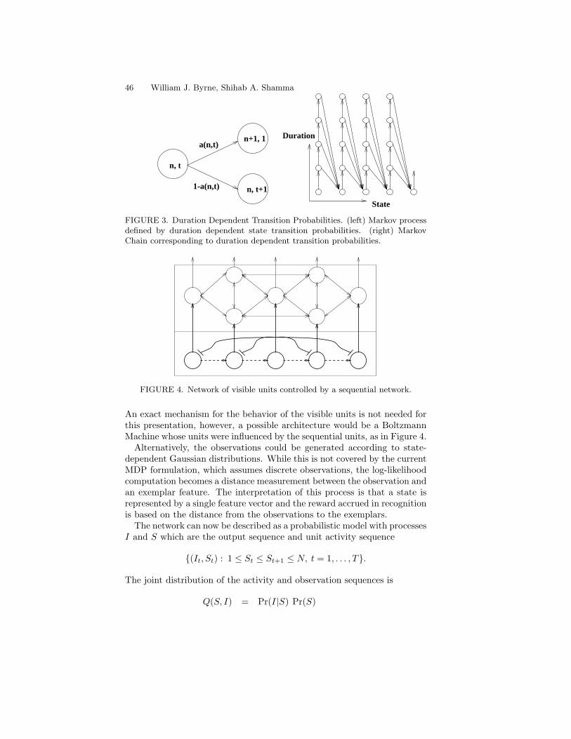
46 William J. Byrne, Shihab A. Shamma
n, t
n+1, 1
n, t+1
a(n,t)
1-a(n,t)
Duration
State
FIGURE 3. Duration Dependent Transition Probabilities. (left) Markov processdefined by duration dependent state transition probabilities. (right) MarkovChain corresponding to duration dependent transition probabilities.
FIGURE 4. Network of visible units controlled by a sequential network.
An exact mechanism for the behavior of the visible units is not needed forthis presentation, however, a possible architecture would be a BoltzmannMachine whose units were influenced by the sequential units, as in Figure 4.
Alternatively, the observations could be generated according to state-dependent Gaussian distributions. While this is not covered by the currentMDP formulation, which assumes discrete observations, the log-likelihoodcomputation becomes a distance measurement between the observation andan exemplar feature. The interpretation of this process is that a state isrepresented by a single feature vector and the reward accrued in recognitionis based on the distance from the observations to the exemplars.
The network can now be described as a probabilistic model with processesI and S which are the output sequence and unit activity sequence
(It, St) : 1 ≤ St ≤ St+1 ≤ N, t = 1, . . . , T.
The joint distribution of the activity and observation sequences is
Q(S, I) = Pr(I|S) Pr(S)

3. Neurocontrol in Sequence Recognition 47
=T∏
t=1
bSt(It)
N−1∏n=1
dn(τn).
The distribution has the form of a Hidden Markov Model, specifically, avariable duration Hidden Markov Model (VDHMM) [Lev86], where theprobability of leaving a state depends on how long the system has been inthat state.
The duration distribution dn determined by the network parameters hassome attractive properties. When k ≈ 0, it has a peak at τn ≈ wn
g , whichspecifies the most likely duration. Additionally, for wn
g fixed, the varianceof the unit activity duration decreases as g increases. This can be used toincorporate uncertainty about event duration in the network model.
In a non-variable duration HMM, the state duration probability has theform (1− a)τ−1a, where a is the probability of remaining in a state. It hasbeen argued that other distributions, such as Gaussian and Gamma dis-tributions, provide better temporal modeling. The distribution that ariseshere enjoys the two main features of the previously used distributions,namely the non-zero maximum likelihood duration and an adjustable vari-ance. The difference between this model and other VDHMMs is that theduration distribution is not chosen beforehand - dn(τ) doesn’t have a closedform expression - but arises from the state transition mechanism.
When k is not negligible, the potential of unit n+1 when excited by unitn eventually approaches
xt(n + 1) = −wn + c + g/k
so that an(τ), the probability of unit n + 1 activating, approaches
K =1
1 + e−−wn+c+g/k .
Since an(τ) approaches K for large τ , the distribution dn falls off as(1−K)τ (Equation 7). This shows the importance of the excitation channeldecay parameter k. It can be used to control the tail of the state durationdistribution.
Two examples of model density durations are presented in Figure 5. Thedurations of 7500 instances of the phonemes /iy/ and /n/ were obtainedfrom the TIMIT database. Model fits are plotted along with the sampledensities. The parameter k is particularly valuable in fitting the exponen-tial decay often described in phoneme duration histograms.
Training this network is discussed in Chapter 3 of [Byr93]. The EMalgorithm is used to train it as a VDHMM [Lev86] under a maximumlikelihood criterion. This training problem is developed in an informationgeometric framework similar to that used to describe Boltzmann Machinelearning in [Byr92]. Other neural training schemes based on sequentialapproximations to the EM algorithm are also possible [WFO90]. In general,

48 William J. Byrne, Shihab A. Shamma
0 20 40 60 80 100 120 140 1600
0.5
1
1.5
2
2.5
3
3.5
4x 10⁻²
Frame - 2msec step, 20msec window. 16Khz sampling
Model Duration Density and /iy/ Duration Histogram
k = 0.1, w = 11.0, g = 0.85, c = 3.0
0 10 20 30 40 50 60 70 800
1
2
3
4
5
6x 10 -2
Frame - 2msec step, 20msec window. 16Hkz sampling
Model Duration Distribution and /n/ Duration Histogram
k = 0.18, w = 12.0, g = 1.25, c = 3.0
FIGURE 5. Modeling sample duration histograms computed from phoneme du-rations found in the TIMIT database: 6950 instances of /iy/ (top); 7068 instancesof /n/ (bottom).

3. Neurocontrol in Sequence Recognition 49
Dynamical State Network
Observation Process
I(t)
RecognitionControl
andScoringProcess
FIGURE 6. Dynamical Network Architecture Embedded in a Sequence Recog-nizer
modeling duration dependent transition probabilities is difficult, howeverthere has been previous work using neural architectures to address thisproblem [GS89].
Similar networks have been presented elsewhere [RT91, BT91], and ingeneral, dynamic neural networks intended for sequence recognition andproduction have been widely studied [DCN87, Kle86, SK86, BK91]. Thenetwork presented here has the benefit that individual parameters can beassociated with desirable aspects of the network behavior. The gain param-eter g determines the variance of the duration distribution, for example,the inhibition profile determines the relative duration of each units activ-ity, and the decay factor k in the directed excitation channel is used inmodeling the duration distribution tail, as described above.
In source mode, the gain function g is fixed and the state progressionis a random function of the state (n, τ). In use as a recognizer, the gainfunction g is used to control the state progression. To force a change instate from (n, τ) to (n + 1, 1), g is set to a very large value, so that thedirected excitation immediately activates the next unit in the sequence.Otherwise g is kept small so that the current unit remains active. Thisarchitecture is illustrated in Figure 6.
6 Neurocontrol in sequence recognition
Thus far, two topics have been discussed. MLSS sequence recognition withlimited future information has been formulated as a Markov Decision Prob-lem and a stochastic neural architecture intended for modeling observationsequences has been introduced. In this section, a controlled sequence rec-ognizer built on this network architecture will be described.

50 William J. Byrne, Shihab A. Shamma
As described in the previous section, the hidden process of the dynamicalnetwork is a first order Markov process with state St = (n, τ)t. While thisis more complicated than the formulation of section 4.2 which is based ona simple Markov process, the recognizer and control rule are formulatedidentically.
The following conditional probability can be computed recursively
α(n, τ)ht = Pr(St = (n, τ)t | It+h
1 )
which is denoted αht = Th(It+h
t , αht−1), as before. The statistics (It+h
t , αht )
again form a first order Markov process. The joint source-recognizer de-scription is as in Equation 4.
The specification of the optimum recognition control is as presented ear-lier (Equation 5). While the MDP formulation proves the existence of anoptimum rule and provides methods to construct it, it is impractical tosolve explicitly for the control rules. However, the MDP formulation de-scribes the input to the control rule, i.e. how the observations should betransformed before presentation to the controller. According to this for-mulation, the optimum control Ut should be a function of (αh
t , It+ht , Rt).
The control rule which is produced as a function of the source-recognizerstate is unknown, however the MDP formulation specifies that it does exist.Here, a neural network can be trained in an attempt to approximate it.
A set of training sequences is assumed to be available for the model. Forexample, if a network is to be trained to model the digit “nine”, utter-ances of “nine” form the training set. After the network has been trained,the Viterbi algorithm is used to find the best hidden state sequence foreach training sequence. The training sequences and their correspondingMLSSs form a training set which can be used to build a neural networkto implement the recognizer control rule. The source-recognizer statisticsare accumulated recursively, and the recognizer control rule neural networkis trained to implement the control which generates the Viterbi sequence.This is illustrated in Figure 7.
Experimental Results
A small, speaker independent, isolated digit speech recognition experimentwas performed. The observations used were vector quantized features ob-tained from the cochlear model as described in [BRS89]. The features werecomputed at a frame rate of 20 msec and a step size of 2 msec and quan-tized using a 32 codeword vector quantizer. The speech taken from the TIConnected Digits database, and networks were trained for each of the tendigits using ten utterances from ten different male speakers (10 utterancesfrom 10 speakers). The recognition score testing on ten utterances from tenother speakers using the Viterbi algorithm was approximately 95% correct.
From the Viterbi segmentation, a recurrent neural network was trained

3. Neurocontrol in Sequence Recognition 51
Observations
Sequential Network
State DependentScoring Process
LikelihoodScore
RecognitionControlNet
AlphaRecurrent
NeuralNetwork
Observations
Sequential Network
State DependentScoring Process
LikelihoodScore
RecognitionControl
NetAlpha
RecurrentNeural
Network
Viterbi Algorithm
I
I (I,a)
(I,a)
FIGURE 7. Viterbi algorithm supplying recognizer control law as training target(top); neurocontrol implementation of recognition control law (bottom).

52 William J. Byrne, Shihab A. Shamma
to implement the recognition control law. The network consisted of twohidden layers with four units in the first hidden layer and 2 units in thesecond layer. Five frames (h = 5, 10.0 msec) of future information wasprovided to the recognizer and a discounting parameter β = 0.9 was cho-sen. Using this neurally implemented recognition control law, recognitionperformance of approximately 93% correct was obtained.
This experiment is presented as an example of an application of the MDPformulation of MLSS sequence recognition and is far from conclusive. Whilepromising, as currently implemented in software on conventional comput-ers, the computational burden in training and testing prohibits evaluatingthe performance on large problems. However, it is hoped that this for-mulation might prove valuable both in investigations into the behavior ofsuboptimal approximations to the Viterbi algorithm and to prompt furtherinvestigation into applications of neurocontrol in sequence recognition.
7 Observations and Speculations
As MDP sequence recognition has been formulated, it has been assumedthat the observations are produced by the source HMM Q which is alsoused to define the likelihood criterion LQ. A more general formulation ispossible. A more complex source could be used, for example, such as amixture of HMM sources. The only restriction is that it must be possibleto accumulate statistics so that the recognizer can be described as drivenby a Markov process.
Model training and training of the neural network which implements thecontrol law were presented as separate procedures. In many applicationsof neurocontrol estimation of model parameters and the control law areperformed simultaneously [BSS90]. Such a formulation is possible here, andcould be based upon sequential versions of the EM algorithm [WFO90].
7.1 The Good Recognizer Assumption
An interesting simplification which follows from the MDP formulation ofMLSS sequence recognition problem arises from the following assumption.If the recognizer state Rt is assumed to be a very good estimate of thesource hidden state St, the problem is greatly simplified. The assumptionis
Pr(St = n | It+h1 , Rt) =
1 Rt = n0 otherwise .
This assumption leads to a drastic reduction in the source-recognizer statedimension and to an interesting relationship between the source and recog-nition controls.

3. Neurocontrol in Sequence Recognition 53
The first simplification due to the assumption is the elimination of thestatistic αt. Becauseαh
t (n) = Pr(St = n|It+h1 ), and Rt is a function of It+h
1 , αht (n) = δn(Rt).
Therefore αt is constant for fixed Rt . As a result, the optimum valuefunction V (r, i, α) is a function of r and i alone.
Similarly, the recursive computation of the likelihood term involving It+ht
is also simplified. Note that Rt+1 is a function of It+ht and Rt, since the
control is applied at time t to determine the next recognizer state, so that
Pr( It+1+ht+1 = ih+1
1 | It+h1 = ih1 ) = Pr( It+h+1 = ih+1 | It+h
1 = ih1 )
=∑
n
Pr(It+1+h = ih+1 |St+1, It+h1 ) Pr(St+1 = n | It+h
1 = ih1 )
=∑
n
Pr(It+1+h = ih+1 |St+1, It+ht+2 = ih2 ) Pr(St+1 = n |Rt+1, It+h
1 )
Using φh(i|St+1) to denote the probabilityPr(It+1+h = ih+1 |St+1, It+h
t+2 = ih2 ), the above reduces to
Pr( It+1+ht+1 = i | It+h
1 = ih1 ) = φh(i |Rt+1).
The accumulated statistics αht are no longer used in computing
Pr( It+1+ht+1 = i | It+h
1 ). Instead, this term is approximated byPr( It+1+h
t+1 = i | It+ht+2 , St+1), where the recognizer state Rt+1 is used as an
estimate of the source state St+1.Modifying the optimum value equations to include this simplification
yields
V h(r, i) = maxu
v(r, i1;u) + β∑i′
V h(f(r;u), i′) φh( i′ | f(r;u) ) .
This assumption leads to interesting interpretations of the control rules.Because the recognition control u appears directly in the source observationstatistics, the recognizer acts as if it directly controls the source sequenceproduction. This suggests a close link between the production and recog-nition processes. When the recognition process is accurate, the recognitioncontrol law recovers the source control law best suited to produce the ob-servation sequence. This suggests that this formulation of sequence recog-nition may provide an avenue for the use of speech production mechanisms,or articulatory models, in speech recognition.
Control Rules
The value functions which result from the simplifying assumption can besolved fairly easily. The Good Recognizer assumption removes the de-pendence upon the accumulated statistics α so that the dimensionality ofthe value functions is greatly reduced. It is possible to solve them in a

54 William J. Byrne, Shihab A. Shamma
left-to-right manner: V (r, i) depends upon itself and V (r + 1, i). This ismade particularly easy when the recognizer state r is expanded to includethe state-duration τ . In this case, the Markov chain allows only the twotransitions (r, τ) → (r, τ + 1), (r + 1, 1). In this case, V (r, τ, i) dependssolely upon V (r, τ + 1, i) and V (r + 1, 1, i). V (N, τ, i) is solved first andthen V (r, τ, i) is solved for decreasing r. In practice, this requires pickinga maximum value of τ . The V (N, τ, i) can be then be solved directly; anapproximation is to pick V (N, τmax, i) at random and solve backwards fordecreasing τ .
Consider the h = 1 case. Here, i = (i1, i2) andφ1(i|St+1) = Pr(It+2 = i2|St+1). The value functions are presented herewith the reward expressed in likelihood form
V (N, τ, i) = log(1 − aN (τ))bN (i1) +
β∑i3
φ1((i2, i3)|N)V (N, τ + 1, (i2, i3))
V (r, τ, i) = maxlog(1 − ar(τ))br(i1) +
β∑i3
φ1( (i2, i3) | r)V (r, τ + 1, (i2, i3)) ,
log ar(τ) br(i1) +
β∑i3
φ1( (i2, i3) | r + 1 )V (r + 1, 1, (i2, i3)) .
Denoting∑
i2φ1( (i1, i2) | r)V (r, τ, (i1, i2)) as V (r, τ, i1), the decision rule
can be simplified. Suppose that at time t, the recognizer is in state (r, τ)and the observation symbol It+1 becomes available. The recognition controllaw is chosen according to
V (r, τ + 1, It+1) − V (r + 1, 1, It+1)u = 0≥
<u = 1
1β
log1 − ar(τ)
ar(τ).
The recognition control law becomes a fairly simple table lookup which,using the next available observation, is based upon comparing expectedrewards against a duration-dependent threshold. This could easily be im-plemented in a neuro-control architecture.
Experiments have been carried out using recognition control rules basedupon this simplification. However, the results were unsatisfactory. Forwhatever reasons, but most likely due to overly optimistic nature of theassumption, the recognizers behaved poorly. Typical behavior was to eitherremain in the initial state or move to the final state as quickly as possible.This assumption may yet prove valuable however, as it suggests methodsby which the dimensionality of the value functions and control rules may

3. Neurocontrol in Sequence Recognition 55
be reduced. A topic of future interest might be the investigation of other,not so drastic, approximating assumptions which might yield reductions incomputational cost without too much loss in performance.
7.2 Fully Dynamic Sequential Behavior
As presented in Section 5, the dynamical network is suitable for recogniz-ing single, individual sequences, such as words spoken in isolation. Whiledetermining the underlying event sequence in such applications is not ofcrucial importance, it has been given as a demonstration of the MDP recog-nition formulation in which local decisions can be made that avoid the useof non-causal dynamic programming algorithms.
The ultimate desired application of the dynamical network is in iden-tifying subsequences in continuous observation streams as necessary forconnected or continuous speech recognition. To be useful in such appli-cations, the network architecture must be modified. By allowing the finalnetwork unit N to excite the first network unit, the network can be madeto oscillate. After the N th unit has been active, the first unit activates andthe network repeats its pattern sequence. In this way the network behavesas a controlled oscillator.
Oscillatory networks have been used as models of central pattern gener-ation in simple neural systems [Mat87, Mat85, SK86, Kle86]. Such oscil-latory behavior has been investigated in the network presented here andhas been described elsewhere [BRS89]. As in the isolated sequence case,it is desirable to use the dynamical behavior of the network in these morecomplex sequence recognition problems.
In problems in which higher level context must be modeled, such as whensequences can appear as substrings in other sequences, it is hopeful thatlarge networks with cyclic behavior might be built which would capture thecomplexity of the task. Ideally, a “grammar” which describes the problemwould control the cyclic behavior of the network in much the same way thatlanguage models are currently used in HMM speech recognition systems toconstrain the acoustic search.
In such an application, the dynamical network operates in either phase-locked or free-cycling mode. A recognition controller is used to vary theexcitation gain g to induce either of these modes, as described earlier inSection 5. In free-cycling mode, the excitation gain is set to a high value sothat the network progresses quickly through its state sequence. In phase-locked mode, the network progresses through its state sequence at a ratematched to the observed sequence. This is an indication that the observa-tions agree with the network model. Because this behavior is indicated bythe control law itself, the value of g serves as an indication of the matchbetween the observations and the model.
An example of early experiments into this phase-locking behavior is de-scribed here. The dynamical network is intended to synchronize with the

56 William J. Byrne, Shihab A. Shamma
Speech
Control SignalsDynamical State
State-Phoneme
Network
Mapping
Comparator Classification PhonemicError
Signal Extraction
CochlearModel
Feature
Network
FIGURE 8. Dynamical network embedded in a simple phone classifier architec-ture: (top) System architecture; (bottom) Synchronization of a network trainedto recognize “four” to the utterance “nine four two”.
output of phoneme classifiers when the correct word is in the input stream.When incorrect words are in the input, the network should lose synchro-nization and free-cycle.
Feed-forward networks were trained to classify hand-labeled segmentsof spoken digits. The classifier outputs were thresholded to make a bi-nary decision about the identity of the observation, so that the networkis presented with a binary vector of classifier signals. The Hamming dis-tance between the network activity vector and the classifier output is usedas a measure of instantaneous agreement between the observations and therecognizer. The network gain is obtained directly from this agreement mea-surement by simple low-pass filtering. If the network and classifier vectorsare in agreement, the gain will decay, and the network state progressionwill slow. Conversely, if the agreement is poor, the error will drive up thegain, and the network will speed up. Ideally, the network will synchronizeits progression to the rate of the input signal. This network architectureis presented in Figure 8 and preliminary experiments with this system aredescribed in [Byr93]. While the example presented here is simple, it cap-tures the formulation of the intended application of the dynamical networkin sequence recognition.
Constructing a recognition control law to implement the desired controlis a non-trivial task. A topic of future research is to extend the MDPformulation to describe recurrent behavior by multiple networks so that arigorous framework for sequential decisions in connected and continuousspeech recognition can be developed.
8 References
[Bel57] R. Bellman. Dynamic Programming. Princeton UniversityPress, Princeton, N.J., 1957.
[BK91] W. Banzhaf and K. Kyuma. The time-into-intensity-mappingnetwork. Biological Cybernetics, 66:115–121, 1991.
3. Neurocontrol in Sequence Recognition 57
[BM90] H. Bourlard and N. Morgan. A continuous speech recognitionsystem embedding MLP into HMM. In D. Touretzky, editor,Advances in Neural Information Processing 2, pages 186–193,San Mateo, CA, 1990. Morgan-Kaufmann.
[Bri90] J. Bridle. Alpha-nets: a recurrent neural network architecturewith a Hidden Markov Model interpretation. Speech Commu-nication, 9:83–92, 1990.
[BRS89] W. Byrne, J. Robinson, and S. Shamma. The auditory process-ing and recognition of speech. In Proceedings of the Speech andNatural Language Workshop, pages 325–331, October 1989.
[BSS90] A. Barto, R. Sutton, and C. Sutton. Learning and sequentialdecision making. In M. Gabriel and J .Moore, editors, Learn-ing and Computational Neuroscience: Foundations of AdaptiveNetworks, chapter 13, pages 539–602. Bradford, Boston, 1990.
[BT91] P. Bressloff and J. Taylor. Discrete time leaky integrator net-work with synaptic noise. Neural Networks, 4:789–801, 1991.
[Bur88] D. Burr. Experiments on neural nets recognition of spokenand written text. IEEE Transactions on Acoustics, Speech andSignal Processing, 36:1162–1168, 1988.
[BW89] H. Bourlard and C. Wellekens. Speech pattern discriminationand multilayer perceptrons. Computer Speech and Language,3:1–19, 1989.
[Byr92] W. Byrne. Alternating Minimization and Boltzmann Machinelearning. I.E.E.E. Transactions on Neural Networks, 3(4):612–620, 1992.
[Byr93] W. Byrne. Encoding and representing phonemic sequences us-ing nonlinear networks. Ph.D. thesis, University of Maryland,College Park, 1993.
[DCN87] S. Dehaene, J.-P. Changeux, and J.-P. Nadal. Neural Networksthat learn sequences by selection. Proceedings of the NationalAcademy of Science, U.S.A., 84:2727–2731, May 1987.
[Elm90] J. Elman. Finding structure in time. Cognitive Science,14:179–211, 1990.
[FLW90] M. Franzini, K.F. Lee, and A. Waibel. Connectionist Viterbitraining: a new hybrid method for continuous speech recogni-tion. In Proc. ICASSP, April 1990.

58 William J. Byrne, Shihab A. Shamma
[For67] G. Forney. The Viterbi algorithm. IEEE Transactions on In-formation Theory, IT-13:260–269, April 1967.
[GS89] S. Grossberg and N. Schmajuk. Neural dynamics of adaptivetiming and temporal discrimination during associative learn-ing. Neural Networks, 2(2):79–102, 1989.
[Kle86] D. Kleinfeld. Sequential state generation by neural networks.Proceedings of the National Academy of Science, U.S.A.,83:9469–9473, December 1986.
[KM93] V. Krishnamurthy and J. Moore. On-line estimation of Hid-den Markov Models based on the Kullback-Leibler informationmeasure. IEEE Transactions on Signal Processing, 41(8):2557–2573, August 1993.
[Lev86] S. Levinson. Continuously variable duration Hidden MarkovModels for automatic speech recognition. Computer Speechand Language, 1(1):29–46, March 1986.
[Lev93] E. Levin. Hidden Control neural architecture modeling of non-linear time varying systems and its applications. IEEE Trans-actions on Neural Networks, 4(1):109–116, January 1993.
[LG87] R. Lippmann and B. Gold. Neural network classifiers useful forspeech recognition. In Proc. IEEE First International Confer-ence on Neural Networks, pages 417–425, San Diego, CA, June1987.
[Mak91] A. Makowski. ENEE 726. Stochastic Control Class Notes,Dept. Electrical Engineering, University of Maryland, Fall1991.
[Mat85] K. Matsuoka. Sustained oscillations generated by mutuallyinhibiting neurons with adaptation. Biological Cybernetics,52:367–376, 1985.
[Mat87] K. Matsuoka. Mechanisms of frequency and pattern control inthe neural rhythm generators. Biological Cybernetics, 56:345–353, 1987.
[MB90] N. Morgan and H. Bourlard. Continuous speech recognitionusing multilayer perceptrons and Hidden Markov Models. InProc. ICASSP, pages 413–416, Albuquerque, NM, April 1990.
[MO70] H. Mine and S. Osaki. Markov Decision Processes. AmericanElsevier, New York, 1970.

3. Neurocontrol in Sequence Recognition 59
[Mon82] G. Monaham. A survey of partially observable Markov deci-sion processes: theory, models and applications. ManagementScience, 28(1):1–16, January 1982.
[MY72] I. Morishita and A. Yajima. Analysis and simulation of net-works of mutually inhibiting neurons. Kybernetic, 11, 1972.
[NS90] L. Niles and H. Silverman. Combining Hidden Markov Modelsand neural network classifiers. In Proc. ICASSP, pages 417–420, 1990.
[Rab89] L. Rabiner. A tutorial on Hidden Markov Models and selectedapplications in speech recognition. Proceedings of the IEEE,77(2):257–286, February 1989.
[RBH86] L. Rabiner and B.-H.Juang. An introduction to HiddenMarkov Models. IEEE ASSP Magazine, pages 4–16, January1986.
[Ros83] S. Ross. Introduction to Stochastic Dynamic Programming.Academic Press, New York, 1983.
[RT91] M. Reiss and J. Taylor. Storing temporal sequences. NeuralNetworks, 4:773–787, 1991.
[SIY+89] H. Sakoe, R. Isotani, K. Yoshida, K. Iso, and T. Watanabe.Speaker independent word recognition using dynamic program-ming neural networks. In Proc. ICASSP, pages 29–32, Glas-gow, Scotland, May 1989.
[SK86] H. Sompolinsky and I. Kanter. Temporal association in asym-metric neural networks. Physical Review Letters, 57(22):2861–2864, December 1986.
[S.L85] S.Levinson. Structural methods in automatic speech recogni-tion. Proceedings of the IEEE, 73(11):1625–1650, November1985.
[SL92] E. Singer and R. Lippmann. A speech recognizer using radialbasis function neural networks in an HMM framework. In Proc.ICASSP, 1992.
[SLM84] S.Levinson, L.Rabiner, and M.Sondhi. An introduction to theapplication of the theory of probabilistic functions of a Markovprocess to automatic speech recognition. The Bell SystemTechnical Journal, 64(4):1035–1074, April 1984.
[TH87] D. Tank and J. Hopfield. Neural computation by concentratinginformation in time. Proceedings of the National Academy ofScience, U.S.A.: Biophysics, 84:1896–1900, April 1987.

60 William J. Byrne, Shihab A. Shamma
[UHT91] K.P. Unnikrishnan, J. Hopfield, and D. Tank. Connected-digitspeaker-dependent speech recognition using a neural networkwith time-delayed connections. IEEE Transactions on SignalProcessing, 39(3):698–713, March 1991.
[WFO90] E. Weinstein, M. Feder, and A. Oppenheim. Sequential al-gorithms for parameter estimation based on the Kullback-Leibler information measure. I.E.E.E. Transactions on Acous-tics, Speech, and Signal Processing, 38(9):1652–1654, Septem-ber 1990.
[WHH+89] A. Waibel, T. Hanazawa, G. Hinton, K. Shikano, and K. Lang.Phoneme recognition using time-delay neural networks. IEEETransactions on Acoustics, Speech and Signal Processing,37(3):328–339, March 1989.

4
A Learning Sensorimotor Mapof Arm Movements: a StepToward Biological Arm Control
Sungzoon ChoJames A. ReggiaMin Jang
ABSTRACT Proprioception refers to sensory inputs that principally reg-ulate motor control, such as inputs that signal muscle stretch and tension.Proprioceptive cortex includes part of SI cortex (area3a) as well as partof primary motor cortex. We propose a computational model of neocortexreceiving proprioceptive input, a detailed map of which has not yet beenclearly defined experimentally. Our model makes a number of testable pre-dictions that can help guide future experimental studies of proprioceptivecortex. They are, in particular, first, overlapping maps of both individualmuscles and of spatial locations, second, multiple, redundant representa-tions of individual muscles where antagonist muscle length representationsare widely separated and third, neurons tuned to plausible combinationsof muscle lengths and tensions, and finally proprioceptive “hypercolumns”,i.e., compact regions in which all possible muscle lengths and tensions andspatial regions are represented.
1 Introduction
It has long been known that there are multiple feature maps occurring insensory and motor regions of the cerebral cortex. The term feature maprefers to the fact that there is a systematic, two-dimensional representationof sensory or motor features identifiable over the cortical surface. Generally,neurons close to one another in such maps respond to or represent featuresthat are similar. In most cases, neurons or other supraneuronal processingunits (“columns”) have broadly tuned responses, and thus the receptivefields of neighboring units overlap.
Feature maps are conveniently classified as being either topographic orcomputational. A feature map is called topographic when the stimulusparameter being mapped represents a spatial location in a peripheral space,for instance, the location of a point stimulus on the retina or the location ofa tactual stimulus on the skin. A feature map is called computational when
62 Sungzoon Cho, James A. Reggia, Min Jang
the stimulus parameter represents an attribute value in a feature space, forinstance, the orientation of a line segment stimulus or the spatial locationof a sound stimulus [KdLE87, UF88].
Several computational models have been developed to simulate the self-organization and plasticity of these cortical maps, including topographicmaps in somatosensory (SI) cortex [GM90, PFE87, Skl90, Sut92] and com-putational maps in visual cortex [BCM82, Lin88, MKS89, vdM73]. Whilenot without their limitations, these and related models have shown thatfairly simple assumptions, such as a Mexican Hat pattern of lateral corti-cal interactions and Hebbian learning, can qualitatively account for severalfundamental facts about cortical map organization.
To our knowledge, the goal of all past computational models of corticalmaps has been to explain previously established experimental data concern-ing relatively well-defined maps. In contrast, in this paper we develop acomputational model of neocortex receiving proprioceptive input (hereaftercalled “proprioceptive cortex”), a detailed map of which has not yet beenclearly defined experimentally. Proprioception refers to sensory inputs thatprincipally regulate motor control, such as inputs that signal muscle stretchand tension. Proprioceptive cortex includes part of SI cortex (area3a) aswell as part of primary motor cortex [Asa89]. Our model makes a num-ber of testable predictions that can help guide future experimental studiesof proprioceptive cortex. In addition, the results of our simulations mayhelp clarify recent experimental results obtained from studies of primarymotor cortex, a cortical region that is heavily influenced by proprioceptiveinputs [Asa89]. To our knowledge, this is the first computational model ofmap formation in proprioceptive cortex that has been developed.
The overall concern in this paper is with what sensory feature mapscould emerge in cortex related to the control of arm movements. Insightinto this issue is not only of interest in a biological context, but also tothose concerned with control of robotic arms or other engineering controlapplications [WS92]. There have been several previous models of map for-mation with model arms [BG88, BGO+92, Kup88, Mel88, RMS92]. Theseprevious models are different from that described here in that they are usu-ally concerned with visuomotor transformation process of a 3-D reachingarm movement taking place in motor cortex. Thus, they typically use spa-tial location such as xyz-coordinates of an arm’s endpoint as input ratherthan only muscle length and tension as was done here.
Thus, these past models have not been concerned with proprioceptivemap formation.
The role of primary motor (MI) cortex in motor control has been anarea of intense research during the last several years [Asa89]. Recentstudies have discovered a great deal about the encoding of movements inMI [CJU90, DLS92, GTL93, LG94, SSLD88], although many aspects ofthe organization of the MI feature map remain incompletely understoodor controversial (see [SSLD88] for a cogent review). For example, exper-

4. A learning sensorimotor map of arm movements 63
imental maps of MI muscle representations have revealed that upper ex-tremity muscles are activated from multiple, spatially separated regions ofcortex [DLS92]. It has been suggested that this organization may providefor local cortical interactions among territories representing various musclesynergies. While this may be true, the model proprioceptive cortex de-veloped here offers another explanation: that such an organization may besecondary to multiple, spatially separated muscle representation in proprio-ceptive cortex. Proprioceptive input exerts a significant influence on motorcortex [Asa89]. Thus, this model of proprioceptive cortex may help clarifythese and other organizational issues concerning primary motor cortex.
In our work, a model arm provides proprioceptive input to cortex. Ourmodel arm is a substantial simplification of reality: there are only sixmuscles (or muscle groups), there are no digits, there is no rotation at joints,gravity is ignored, and only information about position is considered. Twopairs of shoulder muscles (flexor and extensor, abductor and adductor) andone pair of elbow muscles (flexor and extensor) control and move the modelarm which we study in a three dimensional (3-D) space. Nevertheless,as will be seen, this simplified arm provides sufficient constraints for asurprisingly rich feature map in the cortex.
The resultant feature map consists of regularly spaced clusters of corti-cal columns representing individual muscle lengths and tensions. Corticalunits become tuned to plausible combinations of tension and length, andmultiple representations of each muscle group are present. The map is or-ganized such that compact regions within which all muscle group lengthsand tensions are represented could be identified. Most striking was theobservation that, although not explicitly present in the input, the corticalmap developed a representation of the three-dimensional space in whichthe arm moved.
2 Methods
We first present a neural network model of proprioceptive cortex, its acti-vation mechanism and learning rule. Secondly, the structure of the modelarm and the constraints it imposes on input patterns are given. The modelarm is not a neural model; it is a simple simulation of the physical con-straints imposed by arm positioning. Finally, we describe how we generatethe proprioceptive input patterns from the model arm.
2.1 Neural Network
The model network has two separate layers of units, the arm input layerand proprioceptive cortex layer (or simply “cortical layer” from now on)(see Fig. 1). Each unit in the arm layer competitively distributes its ac-

64 Sungzoon Cho, James A. Reggia, Min Jang
k
l
j
muscle length muscle tension
fully connected
(20x20)
(6) (6)
kjw ljw
Input layer
Cortical layer
FIGURE 1. Neural network. The arm input layer contains six muscle lengthunits and six muscle tension units, whose activation values represent the propri-oceptive inputs of muscle length and tension values. The cortical layer consistsof a grid of 20 × 20 units which represents proprioceptive cortex. Each unitis connected to its six immediate neighboring units (a hexagonal tessellation isused). To remove edge effects, units on the edges are connected with units onthe opposite edges, so the cortical layer effectively forms a torus. The connectionweights from input layer to cortical layer are initially randomly generated froma uniform distribution, then updated through training. The lateral connectionweights between cortical units are constant.

4. A learning sensorimotor map of arm movements 65
tivation to every unit in the cortical layer. Each unit in the cortical layeralso competitively distributes its activation to its neighbors through lateralconnections. Competitive activation mechanisms have been shown to bequite effective in many different applications [RDSW92, RSC91]. With therecent development of learning algorithms for use with competitive activa-tion mechanisms, these activation mechanisms can now be used in a widevariety of applications [CR92, CR93, RSC91]. One distinct feature of acompetitive activation mechanism is its ability to induce lateral inhibitionamong units, and thus to support map formation, without using explicit in-hibitory connections [CR92, RDSW92, Sut92, UF88]. Even with constantweight values for all cortico-cortical connections, a Mexican Hat pattern ofactivation appears in the cortex [RDSW92]. It is this feature that we tryto exploit in map formation at the cortical layer.
The activation level of unit k at time t, ak(t) is determined by 1
dak(t)dt
= csak(t) + (max − ak(t))ink(t) (1)
where
ink(t) =∑
j
okj(t) =∑
j
cp(ap
k(t) + q)wkj∑l(a
pl (t) + q)wlj
aj(t). (2)
This activation rule is same as the rule used in [RDSW92]. The weight onthe connection from unit j to unit k is denoted by wkj , which is assumedto be zero when there is no connection between the two units. Althoughthe weight variable is also a function of time due to learning, it is consid-ered constant in the activation mechanism because activation levels changemuch faster than weights. The constant parameters cs and cp representdecay at unit k (with negative value) and excitatory output-gain at unitj, respectively. The value of cs controls how fast activation decays whilethat of cp determines how much output a unit sends in terms of its activa-tion level. The exponent parameter p determines how much competitionexists among the units. The larger the value of p, the more competitivethe model’s behavior, and thus the greater peristimulus inhibition. Theparameter q (a small constant such as 0.0001) is added to ak(t) for allk, to prevent division by zero (denominator term in Eq. 2) and to influ-ence the intensity of lateral inhibition. The parameter max representsthe maximum activation level. The output okj(t) from unit j to unit kis proportional not only to the sender’s activation level, aj(t), but also tothe receiver’s activation level, ak(t). Therefore, a stronger unit receivesmore activation. Another unit l which also gets input from unit j can beseen as competing against unit k for the output from unit j because thenormalizing factor
∑l∈N (al(t) + q)wlj in the denominator constrains the
1Arm layer units are clamped to the length and tension values computed from random
cortical signals to six muscles, thus the equation applies only to the cortical layer units.

66 Sungzoon Cho, James A. Reggia, Min Jang
sum of the outputs from unit j to be equal to its activation level, aj(t),when cp = 1. The activation sent to unit k, therefore, depends not only onthe activation values of the units from which it receives activation such asunit j, but also on the activation values of its competitors to which unitk has no explicit connections. Since competitive distribution of activationimplicitly assumes that activation values are nonnegative, we used a hardlower bound of zero when we update activation values in Eq. 1 in orderto prevent the activation values from ever going negative. The equationis approximated by a difference equation with ∆t = 0.1. Other parametervalues were determined empirically as follows. For cortical layer units, de-cay constant cs and ceiling max values in Eq. 1 were set to −4.0 and 5.0respectively. Their q and output gain parameter cp values in Eq. 2 were setto 0.001 and 0.9, respectively. For arm layer units, q and cp values in Eq. 2were set to 0.1 and 0.8, respectively. Since arm layer units were clamped,their cs and max values were not relevant. Further details of the activationmechanism can be found in [RDSW92].
2.2 Learning
Connection weights are modified according to competitive learning, a vari-ant of Hebbian Learning that tends to change the incoming weight vectorsof the output units (cortical layer units here) into prototypes of the inputpatterns [RZ86]. The particular learning rule used here is adapted from[Sut92] and [vdM73]:
∆wkj = η[aj − wkj ]a∗k (3)
where
a∗k =
ak − θ if ak > θ0 otherwise (4)
and where parameters η and θ are empirically set to 0.1 and 0.32. Only theweights from the arm layer to the cortical layer are changed by Eq. 3; thecortico-cortical connections are constant. Before training, weights were ran-domly selected initially from a uniform distribution in the range of [0.1,1.0].Updated weights were also normalized such that the 1-norm of the incom-ing weight vector of each cortical unit is equal to that of input patterns (theaverage size of input pattern was empirically found to be 7.45). Insteadof checking at each iteration whether the network reached equilibrium weran the network for fixed number of iterations, 32, which was found toapproximate equilibrium empirically and at this point one step of learningwas done according to Eq. 3.
2.3 Model Arm
Basically, the model arm consists of two segments we call the upper armand lower arm, connected at the elbow. The model arm is fixed at the

4. A learning sensorimotor map of arm movements 67
TABLE 1. Proprioceptive input values for the network. The value inM denotesthe randomly generated neuronal input to muscle M . The values lM and TM
respectively represent the length and tension input values of muscle M .
Joint Angle Muscle (M) Length (lM ) Tension (TM )α π
2 (inB − inD) Abductor sin (12 (π
2 − α)) inB + 0.1 · lBAdductor cos ( 1
2 (π2 − α)) inD + 0.1 · lD
β π2 (inE − inF ) Extensor sin (1
2 (π2 − β)) inE + 0.1 · lE
Flexor cos ( 12 (π
2 − β)) inF + 0.1 · lFγ π
2 (inO − inC) Opener sin (12 (π
2 − γ)) inO + 0.1 · lOCloser cos ( 1
2 (π2 − γ)) inC + 0.1 · lC
shoulder and has only six generic muscles or muscle groups. We assumethat there are four muscles that control the upper arm and two muscles thatcontrol the lower arm. These “muscles” correspond to multiple muscles ina real arm. Abductor and adductor muscles move the upper arm up anddown through 180, respectively, while flexor and extensor muscles move itforward and backward through 180, respectively. These four muscles areattached at points equidistant from the shoulder. The lower arm is movedup to 180 in a plane, controlled by closer (lower arm flexor) and opener(extensor) muscles as described in Fig. 2.
This model arm is a great simplification of biological reality, and is in-tended as only a first effort for modeling feature map formation in theproprioceptive cortex. Neither the dynamics of the arm movement nor theeffects of gravity on the arm are considered. Also the arm is assumed not torotate around the elbow or shoulder joints. Only the positional informationabout the arm is part of the model.
2.4 Proprioceptive Input
Since there is no motor cortex in our model, input activation to musclesmust somehow be generated. We first generate six random numbers whichrepresent input activation to the six muscles that control the model arm.Given this input activation, we compute the expected proprioceptive infor-mation from muscles, i.e., muscle length and tension values. This informa-tion consisting of twelve values is used as input to the proprioceptive cortexin the model. The activation values of arm layer units are clamped to thesevalues. Table 1 shows the formulae from which we compute proprioceptiveinput to the cortical layer.
Fig. 3 shows a generic joint. First, we define the joint angle as a functionof difference between the input activation level of agonist and antagonistmuscles.

68 Sungzoon Cho, James A. Reggia, Min Jang
b
c
γ
x
y
z
B
C(-l/2,0,0)
(0,0,l/2)
(l/2,0,0)
(0,0,-l/2)
α
β
Upper Arm
Lower Arm
Shoulder
Elbow
Hand
adductor
extensor
flexorabductorcloser opener
FIGURE 2. Schematic view of model arm. The model arm is considered as theright arm of a human facing the negative side of the x-axis. The pair of abductorand adductor muscles control the upper arm’s vertical movement around thex-axis through contraction and stretch, with their joint angle denoted as α. Thepair of flexor and extensor muscles control the arm’s horizontal movement aroundthe z-axis, with their angle denoted as β. All four muscles are attached to themidpoint of the upper arm and to imaginary points on either the x-axis or thez-axis. The upper arm can move up to 180 around the two axes, x and z, thus thepossible positions of elbow E define a hemisphere. The pair of opener and closermuscles moves the lower arm up to 180 around only one axis, a time-varyingline perpendicular to the “hand plane” (plane which is generated by the x-axisand elbow) and that passes through the elbow. Thus, the lower arm swings froma position collinear with the upper arm to a “folded” position where hand meetsshoulder. Both muscles are attached to the midpoint of the lower arm and toimaginary points on the extended line of upper arm, both length l/2 apart fromthe elbow. Their joint angle is denoted γ(= HEB) where H and E representhand and elbow positions, respectively and B is the projection of H onto theline segment which is perpendicular to upper arm and on the hand plane. Thepossible positions of hand H define a semicircle with center E and radius l onthe hand plane.
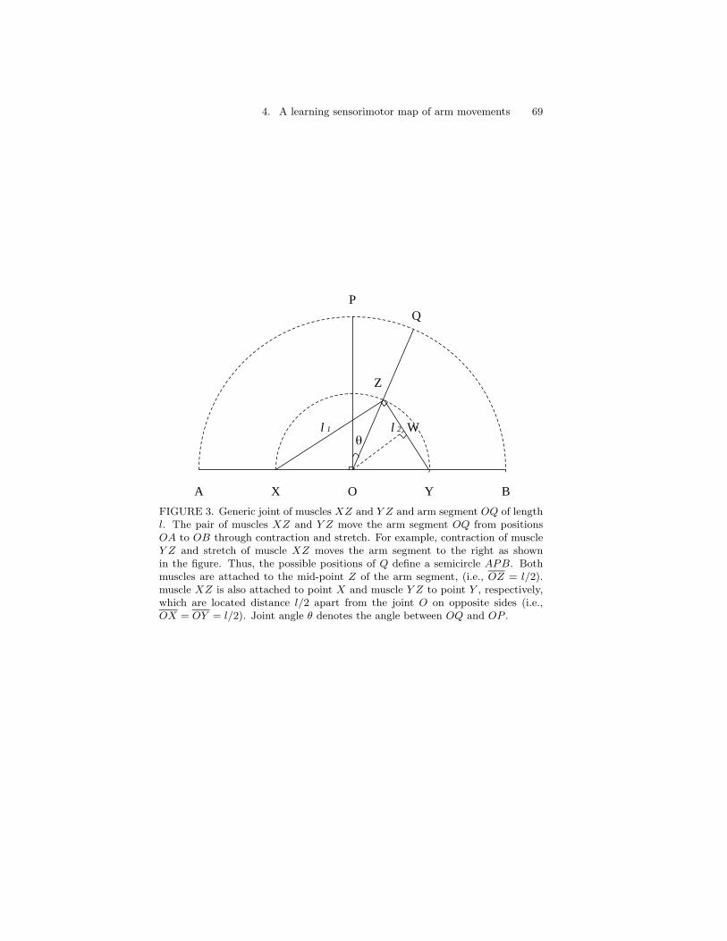
4. A learning sensorimotor map of arm movements 69
21 llθ
W
Z
QP
BYOXA
FIGURE 3. Generic joint of muscles XZ and Y Z and arm segment OQ of lengthl. The pair of muscles XZ and Y Z move the arm segment OQ from positionsOA to OB through contraction and stretch. For example, contraction of muscleY Z and stretch of muscle XZ moves the arm segment to the right as shownin the figure. Thus, the possible positions of Q define a semicircle APB. Bothmuscles are attached to the mid-point Z of the arm segment, (i.e., OZ = l/2).muscle XZ is also attached to point X and muscle Y Z to point Y , respectively,which are located distance l/2 apart from the joint O on opposite sides (i.e.,OX = OY = l/2). Joint angle θ denotes the angle between OQ and OP .

70 Sungzoon Cho, James A. Reggia, Min Jang
Joint angle: Let us denote as inag and inant the input activation levelof agonist and antagonist muscles. Then, the joint angle θ is defined asθ = π
2 (inag − inant).Note that value θ ranges from −π/2 to π/2, exclusive of the end points. Insimulations, values of in are randomly generated from a uniform distribu-tion in [0,1].
Muscle length units in the network model muscle spindle, or stretch re-ceptor inputs, which fire strongly when the muscle is mechanically stretched.We can derive the lengths of the muscles, l1 (=XZ) and l2 (=Y Z) fromthe joint model shown in Fig. 3.
Muscle length: Given joint angle θ and appendage length l as in Fig. 3,muscle lengths l1 and l2 are
l1 = l cos12(π
2− θ) (5)
l2 = l sin12(π
2− θ). (6)
To see this, consider OY Z, an isosceles triangle with OY = OZ = l/2.Let W be on Y Z such that OW ⊥ Y Z, so OWY is a right triangle with
Y OW =12(π
2− θ) (7)
andY W =
l22
. (8)
From Eqs. 7 and 8, we get
sin12(π
2− θ) =
Y W
OY=
l2/2l/2
= l2/l,
thus, we have Eq. 6.Now consider XZY . Point Z is on a semi-circle with center O and
diameter l, so XZY = π2 . Thus, we have
XZ2
+ Y Z2
= XY2
l21 + l22 = l2
l1 =√
l2 − l22.
Substituting Eq. 6 for l2, we have Eq. 5 since 12 (π
2 − θ) ∈ [0, π2 ].
Because of their location serial to muscle fibers, Golgi tendon organsstrongly respond when the muscle actively contracts. Passive stretching ofthe muscle also activates the Golgi tendon organ but not as much [CG85].These observations lead to the following.

4. A learning sensorimotor map of arm movements 71
Muscle Tension: Let ini denote the input activation to muscle i. Then,the muscle tension Ti is defined as
Ti = ini + T · li (9)
where T is a small constant.The first term ini at unit i represents the active portion of the total
tension generated by the muscle. The second term, T li, represents thesecondary sensitivity of the Golgi tendon organ to passive muscle stretch-ing.
Input values to muscles in are uniform random variables whose valuesrange from 0 to 1. However, actual input values to the neural network suchas joint angle, length, and tension are not uniform random variables. Thisis because any arbitrary transformation of uniform random variables doesnot usually result in another uniform random variable. This leads us tothe observation that certain combinations of length and tension values arepresented disproportionally more often during training. For instance, jointangle values near zero will be presented more often than other values.
3 Simulation Results
We present three types of results from this study of map formation in theproprioceptive sensory cortex. First, we show that both length and ten-sion maps formed during training. Second, we characterize these maps bydescribing various redundancies and relationships that appear. Third, wedescribe the map of hand position in three dimensional space that formedeven though there was no explicit input of hand position.
3.1 Formation of length and tension maps
To examine whether maps of muscle length and tension formed duringtraining, we measured which muscle’s length or tension each cortical unitresponded to most strongly. Consider an input pattern where only onemuscle length or tension unit (arm unit) is activated. There are 12 suchinput patterns, because we have six muscle length and six tension units.Since the arm units represent the length and tension of six muscles of themodel arm (flexor and extensor, abductor and adductor in upper arm, andflexor and extensor in lower arm), each of these input patterns correspondsto the unphysiological situation where either length or tension of only onemuscle is activated. For instance, an input pattern of (P, 0, 0, ..., 0) rep-resents the case where the upper arm extensor’s length unit is activated

72 Sungzoon Cho, James A. Reggia, Min Jang
while all other units are not 2These input patterns were not used duringtraining. Nevertheless, they provide an unambiguous and simple methodfor measuring map formation. A cortical unit is taken here to be “tuned”to an arm input unit if the sole excitation of the input unit produced acti-vation larger than a threshold of 0.5 at that cortical unit. A cortical unitis “maximally tuned” to an arm input unit if it is tuned to that input unitand the activation corresponding to that input unit is largest. We deter-mined to which of the six muscles each cortical unit was tuned maximally.This was done with respect to both the length and tension of each muscleindependently.
Fig. 4 shows the maximal tuning of cortical units, before (on the top) andafter (at the bottom) training. Consider, for example, the unit displayed inthe upper left corner of the cortical layer. After training (bottom figures),it was maximally tuned to ‘O’ in the length tuning figure and ‘c’ in thetension tuning figure. This translates into: this unit responded maximallyto the opener with respect to the muscle length, but to the closer withrespect to the muscle tension 3cortical units marked with a “-” characterwere found to be not tuned to the length or tension of any muscle.
The number of untuned cortical units decreased 16% (length) and 30%(tension) with training. The number of cortical units tuned to multiplemuscle lengths and multiple tension lengths after training were 46 and 27,respectively. The number of those units multiply tuned to either length ortension was 230.
Now compare the figures regarding length tuning before and after train-ing (those on the left of Fig. 4). Clusters of units responsive to the samemuscle became more uniform in size after training. The size of clustersranged from 2 to 10 before training, but ranged from 3 to 4 after training,and their shape became more regular. Clusters of units tuned to antagonistmuscles were usually pushed maximally apart from each other during train-ing. Many of these changes are more obvious visually if one considers a mapof just two antagonist muscles. For instance, consider the clusters shown inFig. 5, where only those units in Fig. 4 tuned to upper arm extensor (‘E’)and flexor (‘F’) muscles are displayed. After training, clusters of ‘E”s and‘F”s are pushed maximally away from each other, evenly spaced, and moreuniform in size. The network captures the mechanical constraint imposedby the model arm that two antagonist muscles cannot be stretched at thesame time. This result is representative: clusters of antagonist muscles arepushed apart for other pairs, such as upper arm abductor and adductormuscles (‘B’ and ‘D’) and opener and closer muscles (‘O’ and ’C’).
In the case of tension tuning figures, the results are similar. The size of
2A positive constant P is introduced to make the magnitude of a test input patternsimilar to that of a normalized training pattern whose size was 7.45.
3Implications of this type of ‘multiple tuning to antagonists’ will be explored in thenext section.
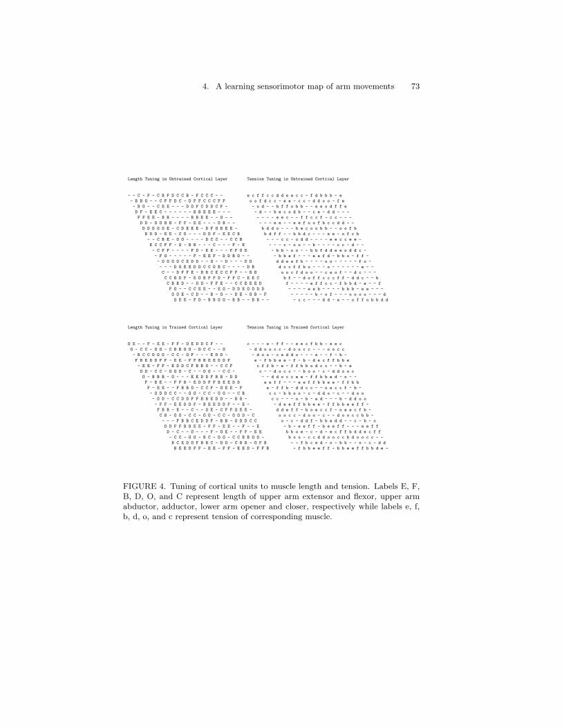
4. A learning sensorimotor map of arm movements 73
Length Tuning in Untrained Cortical Layer Tension Tuning in Untrained Cortical Layer
- - C - F - C B F D C C B - F C C C - - e c f f c c d d e e c c - f d b b b - e
- B B O - - C F F D C - D F F C C C F F o o f d c c - e e - c c - d d o o - f e
- B O - - C E E - - - D O F C D D C F - - o d - - b f f o b b - - e e o d f f e
D F - E E C - - - - - - B B E E E - - - - d - - b e c o d b - - c e - d d - - -
F F E E - B B - - - - B B E E - - O - - - - - - e e c - - f f c c f - c c - - -
D D - D O B B - F F - E E - - - O B - - - - - e e - - e e f o o f b c c d d - -
D D D O O E - C D E E E - D F O B E E - b d d o - - - b e c o o b b - - o o f b
B D D - E E - C D - - - D D F - E E C B b d f f - - b b d c - - - e e - o f c b
- - C B E - O O - - - - D C C - - C C B - - - c c - o d d - - - - e e c c e e -
E C C F F - O - B B - - - C - - - F - E - - - c - o o - - b - - - - c c - d - -
- C F F - - - - F O - E E - - - F F O E - b b - o o - - b b f d d e e o d d c -
- F O - - - - - F - E E F - D D B O - - - b b e f - - - e e f d - b b o - f f -
- O O O O C E D D - - O - - D - - - D D d d e e f b - - - - o o - - - - - f o -
- - - D O E E D D C C O E C - - - - D B d o c f f b o - - - o - - - - - - e - -
C - - D F F E - B B C E C C F F - - B B o o c f d o o - - c e o f - - d c - - -
C C B D F - E O B F F D - F F C - E E C b f - - d o f f c c c f f - d d c - - b
C B B D - - O O - F F E - - C C E E E D f - - - - e f f c c - f b b d - e - - f
F O - - C C E E - - E O - D D E O O D D - - - - e e b - - - - b b b - e e - - -
O O E - C D - - B - O - - D E - O B - F - - - - - b - o f - - - o o o o - - - d
O E E - F D - B B O O - B B - - B B - - - c c - - - d d - e - - o f f o b b d d
Length Tuning in Trained Cortical Layer Tension Tuning in Trained Cortical Layer
O E - - F - E E - F F - O E D D C F - - c - - - e - f f - - e e c f b b - e e c
O - C C - O O - C B B O O - D C C - - O - d d o o c c - d o o c c - - - o o c c
- B C C D O O - C C - O F - - - E D D - - d o o - c e d d o - - - e - - f - b -
F B E D D F F - E E - F F B B E E D D F e - f b b e e - f - b - d e c f f b b e
- E E - F F - E D D C F B B O - - C C F c f f b - e - f f b b o d c c - - b - e
O O - C C - O O D - C - - O O - - C C - c - - d o c c - - b o o - c - d d o o c
O - B B B - O - - - E E D D F B B - D D - - d d o c c e e - f f b b e d - o - -
F - B E - - F F B - E D D F F B E E D D e e f f - - - e e f f b b e e - f f b b
F - E E - - F B B O - C C F - O E E - F e - f f b - d d c c - - o e c c f - b -
- O D D C C - - O O - C C - O O - - C B c c - b b o o - c - d d o - c - - d o o
- O D - C C D D F F B B E D D - - B B - c c - - - o - b - e d - - - b - d d o o
- F F - E E D D F - B E E D D F - - E - - d e e f f b b e e - f f b b e e f f -
F B B - E - - C - - O E - C F F O E E - d d e f f - b o e c c f - o e e c f b -
C B - O O - C C - O O - C C - O O D - C o o c c - d o o - c - - d o o c c b b -
- - - F B B C E D D F - B B - O D D C C o - c - d d f - b b e d d - - c - b - o
D D F F B B E E - F F - E E - - F - - E - b - e e f f - b e e f f - - - e e f f
D - C - - O - - - F - O E - - F F - E E b b o e - c - d - e c f f b d d e c f f
- C C - O O - B C - O O - C C B B O O - b o o - c c d d o o c c b d o o c c - -
B C E D O F B B C - D D - C B B - O F B - - f b c e d - o - b b - - o - c - d d
B E E D F F - E E - F F - E E D - F F B - f b b e e f f - b b e e f f b b d e -
FIGURE 4. Tuning of cortical units to muscle length and tension. Labels E, F,B, D, O, and C represent length of upper arm extensor and flexor, upper armabductor, adductor, lower arm opener and closer, respectively while labels e, f,b, d, o, and c represent tension of corresponding muscle.

74 Sungzoon Cho, James A. Reggia, Min Jang
Extensor/Flexor Length Tuning Extensor/Flexor Tension Tuning
in Untrained Cortical Layer in Untrained Cortical Layer
- - - - F - - - F - - - - - F - - - - - e - f f - - - - e e - - - f - - - - - e
- - - - - - - F F - - - - F F - - - F F - - f - - - - e e - - - - - - - - - f e
- - - - - - E E - - - - - F - - - - F - - - - - - - f f - - - - - e e - - f f e
- F - E E - - - - - - - - - E E E - - - - - - - - e - - - - - - - e - - - - - -
F F E E - - - - - - - - - E E - - - - - - - - - e e - - - f f - - f - - - - - -
- - - - - - - - F F - E E - - - - - - - - - - e e - - e e f - - f - - - - - - -
- - - - - E - - - E E E - - F - - E E - - - - - - - - - e - - - - - - - - - f -
- - - - E E - - - - - - - - F - E E - - - - f f - - - - - - - - - e e - - f - -
- - - - E - - - - - - - - - - - - - - - - - - - - - - - - - - - - e e - - e e -
E - - F F - - - - - - - - - - - - F - E - - - - - - - - - - - - - - - - - - - -
- - F F - - - - F - - E E - - - F F - E - - - - - - - - - - f - - e e - - - - -
- F - - - - - - F - E E F - - - - - - - - - - e f - - - e e f - - - - - - f f -
- - - - - - E - - - - - - - - - - - - - - - e e f - - - - - - - - - - - - f - -
- - - - - E E - - - - - E - - - - - - - - - - f f - - - - - - - - - - - - e - -
- - - - F F E - - - - E - - F F - - - - - - - f - - - - - - e - f - - - - - - -
- - - - F - E - - F F - - F F - - E E - - f - - - - f f - - - f f - - - - - - -
- - - - - - - - - F F E - - - - E E E - f - - - - e f f - - - f - - - - e - - f
F - - - - - E E - - E - - - - E - - - - - - - - e e - - - - - - - - - e e - - -
- - E - - - - - - - - - - - E - - - - F - - - - - - - - f - - - - - - - - - - -
- E E - F - - - - - - - - - - - - - - - - - - - - - - - - e - - - f f - - - - -
Extensor/Flexor Length Tuning Extensor/Flexor Tension Tuning
in Trained Cortical Layer in Trained Cortical Layer
- E - - F - E E - F F - - E - - - F - - - - - - e - f f - - e e - f - - - e e -
- - - - - - - - - - - - - - - - - - - - - - - - - - - - - - - - - - - - - - - -
- - - - - - - - - - - - F - - - E - - - - - - - - - e - - - - - - e - - f - - -
F - E - - F F - E E - F F - - E E - - F e - f - - e e - f - - - - e - f f - - e
- E E - F F - E - - - F - - - - - - - F - f f - - e - f f - - - - - - - - - - e
- - - - - - - - - - - - - - - - - - - - - - - - - - - - - - - - - - - - - - - -
- - - - - - - - - - E E - - F - - - - - - - - - - - - e e - f f - - e - - - - -
F - - E - - F F - - E - - F F - E E - - e e f f - - - e e f f - - e e - f f - -
F - E E - - F - - - - - - F - - E E - F e - f f - - - - - - - - - e - - f - - -
- - - - - - - - - - - - - - - - - - - - - - - - - - - - - - - - - - - - - - - -
- - - - - - - - F F - - E - - - - - - - - - - - - - - - - e - - - - - - - - - -
- F F - E E - - F - - E E - - F - - E - - - e e f f - - e e - f f - - e e f f -
F - - - E - - - - - - E - - F F - E E - - - e f f - - - e - - f - - e e - f - -
- - - - - - - - - - - - - - - - - - - - - - - - - - - - - - - - - - - - - - - -
- - - F - - - E - - F - - - - - - - - - - - - - - - f - - - e - - - - - - - - -
- - F F - - E E - F F - E E - - F - - E - - - e e f f - - e e f f - - - e e f f
- - - - - - - - - F - - E - - F F - E E - - - e - - - - - e - f f - - - e - f f
- - - - - - - - - - - - - - - - - - - - - - - - - - - - - - - - - - - - - - - -
- - E - - F - - - - - - - - - - - - F - - - f - - e - - - - - - - - - - - - - -
- E E - F F - E E - F F - E E - - F F - - f - - e e f f - - - e e f f - - - e -
FIGURE 5. Tuning of cortical units to length and tension of upper arm extensorand flexor muscles only. The same set of labels defined in Fig. 4 are used.

4. A learning sensorimotor map of arm movements 75
clusters became more uniform. However, the clusters of antagonistic mus-cles were not separated maximally apart. In fact, some antagonist clusterswere located adjacent to each other. This is due to the fact that unlikewith muscle lengths, there are no constraints preventing two antagonistmuscles from contracting at the same time. Co-contraction of antagonistmuscles is employed when a stiffer joint is necessary, for instance, to ensurethe desired position when unexpected external forces are present [CG85].
3.2 Relationships
Additional evidence of the trained network’s capturing of the mechanicalconstraints imposed by the arm is found among those cortical units whichare tuned to multiple proprioceptive inputs (i.e., activation over 0.5 formultiple test patterns, each of which corresponds to an input unit). Suchmultiple tuning could potentially not be compatible with physiological con-straints. For instance, it seems unlikely that a cortical unit would be tunedto both a muscle’s length and to its tension together since a muscle tendsnot to contract (high tension) and lengthen simultaneously. Another im-plausible case would be when a cortical unit is tuned to lengths of twoantagonist muscles since they cannot be stretched at the same time.
Table 2 shows the number of implausible multiple tuning cases found inthe network before and after training. For instance, pair (E,F) representsthe number of cortical units which are tuned to both ‘E’ (length of upperarm extensor) and ‘F’ (length of upper arm flexor), and pair (B,b) rep-resents the number of cortical units which are tuned to both length andtension of the upper arm abductor muscle. Each entry represents the num-ber of cortical layer units which were tuned to a physiologically implausiblepair of arm layer units. Entries in the top row show the number of unitsbefore training and those at the bottom row after training. Before training,a total of 69 cortical units were tuned to implausible pairs. After trainingnone of the cortical units had implausible tuning. This clearly shows thatthe trained network captured the physiological constraints imposed by themechanics of the arm by eliminating implausible multiple tuning effectsintroduced by random initial weights.
Tuning of units to some multiple proprioceptive inputs, on the otherhand, could be compatible with the constraints imposed by the mechanicsof the model arm. For instance, in Section 3.1, we considered the unitshown on the left upper corner in Fig. 4 c and 4 d, which is tuned to boththe length of the opener and to the tension of the closer. This unit is, inthat sense, tuned to the contraction of a single muscle, the closer. Con-traction of this muscle increases its arm tension (c) and also increases thelength of its antagonist muscle, the opener (O). Table 3 shows the numberof the cortical units tuned to specific plausible tuning pairs, with the toprow being before training and the bottom row being after training. Thetuning pairs follow the same convention used in Table 2. The pair (E, f),

76 Sungzoon Cho, James A. Reggia, Min Jang
TABLE 2. Numbers of implausibly tuned cortical layer units. Uppercase lettersrepresent muscle length while lowercase letters represent muscle tension.
TuningPairs
E,F B,D O,C E,e F,f B,b D,d O,o C,c total
Beforetraining
7 5 6 6 10 7 9 9 10 69
Aftertraining
0 0 0 0 0 0 0 0 0 0
TABLE 3. Numbers of plausibly tuned cortical units
TuningPairs
E,f F,e B,d D,b O,c C,o total
Aftertraining
12 13 8 6 2 6 47
Aftertraining
42 37 18 35 35 33 200

4. A learning sensorimotor map of arm movements 77
for instance, represents the extensor’s length and flexor’s tension, thus con-traction of the upper arm flexor. Those cortical units which were also tunedto implausible pairs were not counted here even though they might also betuned to contraction of a plausible pair. The data ‘before training’ showsthe effect of randomness of initial weights. Training increased the numberof such cortical units by more than four times. This effect is clearly illus-trated in Fig. 5 c. and d.(compare left (c.) illustration with correspondingright (d.) illustration).
After training, the map can be viewed as being organized into fairlycompact contiguous regions where all possible features are represented ineach region. For instance, the region of about 30 units in the lower leftcorner of the upper right quadrant (Fig. 4 c. and d.) illustrates thisespecially clearly: it has units tuned to every possible muscle length andtension. Such an organization is reminiscent of hypercolumns in visualcortex and quite different from that seen with past cortical maps of touchsensation [GM90, PFE87, Sut92].
3.3 Formation of hand position map
Recall that the sole input information to the model cortex is length andtension information from each of the six muscle groups that control armposition. In other words, there is no explicit input information about the“hand” position in the three dimensional space in which it moves. To assesswhat, if any, kind of map of three dimensional hand position develops incortex, we divided up the hand position space into 27 cubicles (three seg-ments for each axis), computed an ‘average’ hand position for each cubicle,presented the input patterns corresponding to the average hand positions,and determined to which of these 27 test input patterns each cortical unitis maximally tuned. We considered also for each cortical unit to which ofthe three segments of x, y, and z axes it is tuned. In this scheme, the x, y,and z axes are divided into three equal-length segments (Fig. 6). We chosethis particular division of space based on the facts that a large number ofthe training patterns were covered by the resulting 27 cubicles (86%) andthat every cubicle contains at least one training pattern 4
A cubicle is identified as a triplet (i, j, k) where values of i, j, and kdenote the location of the cubicle as
i =
1 if Hx ∈ [−2,−1.2]2 if Hx ∈ [−1.2,−0.4]3 if Hx ∈ [−0.4, 0.4]
j =
1 if Hy ∈ [−0.4, 0.4]2 if Hy ∈ [0.4, 1.2]3 if Hy ∈ [1.2, 2.0]
4The training patterns were not evenly spaced.

78 Sungzoon Cho, James A. Reggia, Min Jang
x = 0.4
x = -0.4
x = -1.2
x = -2.0
y = -0.4 y = 0.4 y = 0.8 y = 1.2
z = -1.2
z = -0.4
z = 0.4
z = 1.2
FIGURE 6. Division of hand position space into 27 cubicles. The x axis wassegmented into three sections X1, X2, and X3 of [−2,−1.2], [−1.2,−0.4], and[−0.4, 0.4], respectively. The y axis was segmented into three sections Y1, Y2, andY3 of [−0.4, 0.4], [0.4, 1.2], and [1.2, 2.0], respectively. The z axis was segmentedinto three sections Z1, Z2, and Z3 of [−1.2,−0.4], [−0.4, 0.4], and [0.4, 1.2], re-spectively.

4. A learning sensorimotor map of arm movements 79
k =
1 if Hz ∈ [−1.2,−0.4]2 if Hz ∈ [−0.4, 0.4]3 if Hz ∈ [0.4, 1.2]
where hand position is (Hx,Hy,Hz). For each cubicle (i, j, k), the averagehand position was calculated from the training samples whose resultanthand positions were within the boundaries of the cubicle, and the corre-sponding muscle lengths and tensions were computed. Note, however, thatonly muscle lengths are determined uniquely, given hand positions: muscletensions are not unique. For simplicity, we chose the tension values suchthat the total tension at each joint was either maximal or minimal. Weran the 27 resulting testing patterns with the already trained network andobserved each cortical unit’s activation. Since we get similar results frommaximal tension and minimal tension patterns, we present the results frommaximal tension patterns only from now on.
Figs. 7 and 8 show the cortical units’ spatial tuning to arm locationbefore and after training, respectively. Tuning after training clearly showmap formation.
There are also clear relationships between spatial position and specificproprioceptive inputs in the map. To understand this, recall that musclelength and hand positions are jointly involved in a set of mechanical con-straints imposed by the model arm. For example, the contraction of theadductor muscle, and thus the stretch of its antagonist abductor muscle,positions the elbow and hand below the shoulder. This translates into thehand position’s z-coordinate being negative (namely segment Z1 in Fig. 6).In other words, a stretched abductor muscle is very likely to correlate withhand position being in Z1
5 Stretching of the adductor muscle, on theother hand, is very unlikely to place the hand in Z1, but is very likely tobe correlated with the hand position in Z3 (i.e., a positive z-coordinate).Another similar constraint is that the contraction of the upper arm flexormuscle, and thus the stretching of its antagonist upper arm extensor mus-cle, tends to position the elbow in front of the body, resulting in the handbeing placed very far in front of the body. This translates to the hand posi-tion’s x-coordinate being very negative (i.e., in segment X1, also defined inSec. 3.3). Therefore, the stretch of the upper arm extensor is very likely toposition the hand in X1. In short, the mechanics of the model arm imposesconstraints on the relations between muscle length and hand positions suchthat there are certain pairs of muscle and hand positions which are verylikely to happen simultaneously and that there are some other pairs whichare not likely to happen simultaneously.
To see if the network learned these types of constraints, we calculatedthe number of cortical units which were tuned both to stretch of a muscleand to various segments of the hand positions of all three axes, both be-
5Recall that the model arm segments do not rotate.

80 Sungzoon Cho, James A. Reggia, Min Jang
X-direction Tuning in Untrained Cortical Layer
2 1 1 3 3 3 3 1 3 3 3 - - 3 2 1 1 1 - 3
1 1 3 1 1 1 1 1 1 2 2 - - 2 3 3 1 2 2 3
3 2 1 1 1 1 2 2 1 2 3 3 3 3 3 1 1 1 - 2
3 3 1 - 2 2 3 3 1 3 3 3 2 - 1 1 1 1 2 3
2 1 - 2 2 3 3 1 1 3 2 2 2 1 1 2 2 2 3 2
1 3 - 3 3 3 2 - 1 2 1 1 1 1 3 2 2 - 1 2
3 3 2 3 1 2 2 1 1 1 1 2 2 3 3 2 2 1 1 3
2 3 1 1 1 1 2 - - 1 1 2 2 2 1 1 1 2 2 3
3 2 1 2 1 2 1 1 1 1 3 2 3 1 1 2 1 1 2 2
1 2 2 2 3 1 1 2 3 3 3 2 1 1 2 2 2 2 3 2
2 3 3 2 2 3 3 2 2 2 2 1 1 2 1 1 3 3 3 1
3 3 3 2 1 1 2 2 2 2 1 1 2 1 1 1 3 3 2 1
3 3 2 3 1 1 1 2 3 - 1 - - 2 1 1 3 2 1 1
3 3 2 2 2 2 3 3 1 1 1 1 1 1 1 3 2 2 2 2
- 3 3 2 3 3 3 1 3 3 1 1 1 - 3 3 2 2 2 2
1 3 3 3 3 3 2 1 3 3 3 2 2 3 3 3 3 3 2 1
2 3 3 - 3 1 1 2 2 3 3 2 1 3 3 2 3 3 2 1
2 3 - - 2 1 2 1 1 3 1 1 1 1 2 2 2 2 2 2
3 3 2 1 2 3 1 1 1 1 3 1 1 1 2 2 2 3 2 2
3 1 1 1 3 3 3 1 1 3 3 - - 2 2 2 1 - - 3
Y-direction Tuning in Untrained Cortical Layer
2 1 2 3 2 1 1 3 1 1 2 - - 1 2 1 1 1 - 3
2 3 2 2 1 2 3 2 1 2 1 - - 1 3 3 1 3 3 3
2 3 2 2 1 2 3 2 1 1 2 2 1 2 1 3 3 2 - 3
3 3 1 - 2 3 2 1 2 1 2 1 1 - 2 3 2 1 1 1
3 1 - 1 1 2 1 3 3 3 1 1 1 2 2 1 1 1 1 2
1 1 - 2 1 1 2 - 3 3 3 1 1 1 2 2 2 - 3 2
1 1 1 2 2 1 1 1 1 3 1 1 1 1 3 3 3 2 2 2
1 3 2 1 1 2 2 - - 1 1 1 1 3 3 3 2 3 3 2
3 3 1 1 3 2 2 1 1 2 3 2 1 3 3 1 2 2 2 2
2 2 1 1 2 3 1 1 1 2 3 3 3 2 1 1 2 2 1 2
3 3 2 1 3 3 3 2 1 3 3 3 1 2 1 1 3 2 1 3
3 3 1 1 2 2 3 2 1 3 1 1 1 1 1 3 3 1 1 3
3 3 2 3 1 2 3 1 1 - 3 - - 3 3 1 3 2 1 3
3 3 1 2 3 3 3 3 2 3 3 2 2 2 1 3 2 3 3 3
- 3 2 2 2 3 3 3 3 1 2 1 1 - 3 1 2 3 3 3
2 3 2 1 1 1 1 2 2 1 2 2 2 3 2 2 3 3 3 1
3 1 2 - 1 3 2 3 3 1 1 1 1 3 1 2 1 2 2 1
2 1 - - 3 3 1 2 2 1 1 2 3 3 1 2 2 1 1 2
2 2 1 2 2 3 1 3 3 1 2 1 3 1 3 2 1 1 1 1
2 1 1 1 2 3 1 3 3 1 2 - - 2 3 3 1 - - 1
Z-direction Tuning in Untrained Cortical Layer
2 2 1 1 2 2 2 2 1 1 2 - - 2 1 1 3 3 - 2
3 1 1 1 2 2 2 1 1 3 3 - - 1 1 3 3 1 1 3
2 1 1 1 3 3 1 2 1 3 2 1 1 1 3 3 1 1 - 3
1 1 1 - 3 1 2 2 1 3 2 1 1 - 3 3 1 1 2 2
2 1 - 3 3 2 2 1 2 1 2 1 1 3 3 2 1 1 2 2
2 2 - 3 3 2 1 - 3 2 1 1 3 3 2 2 1 - 3 3
2 2 1 3 1 1 1 3 3 2 2 3 3 3 3 1 1 1 3 3
2 2 2 1 2 2 3 - - 1 2 3 3 3 2 1 1 1 2 3
1 2 3 3 3 2 1 1 1 2 2 1 1 2 1 2 1 2 2 1
2 3 3 2 2 1 1 1 2 1 1 1 3 3 1 2 2 2 1 1
2 3 3 2 3 1 1 1 2 2 3 2 2 3 3 2 2 1 2 1
3 2 1 3 3 1 1 3 3 3 1 2 2 3 3 2 2 3 2 3
1 1 1 2 1 2 2 3 3 - 1 - - 1 1 2 3 1 3 3
1 1 1 1 2 2 2 3 3 1 1 1 1 1 2 1 1 2 3 1
- 1 1 2 2 1 2 3 2 1 1 1 1 - 1 1 2 3 1 1
1 2 3 2 1 1 1 2 2 1 1 1 1 1 1 2 3 1 1 1
1 3 3 - 1 1 1 3 3 3 3 2 2 1 2 3 3 1 2 1
1 3 - - 3 1 3 3 3 3 2 2 2 1 3 3 1 1 2 2
1 2 3 3 3 3 3 3 3 2 1 1 1 3 3 1 1 2 1 1
2 1 2 2 3 3 2 3 3 1 2 - - 2 2 1 1 - - 1
FIGURE 7. Tuning of untrained cortical units to hand position in each direction,x, y, and z. Each unit is labeled such that the corresponding element of cubicle(i, j, k) is displayed when the unit is maximally tuned to the hand position fromthe cubicle.

4. A learning sensorimotor map of arm movements 81
X-direction Tuning in Trained Cortical Layer
2 - 2 3 3 2 2 - - 3 3 2 2 2 1 1 3 3 2 2
3 - 2 2 2 2 2 - 2 2 2 2 2 2 2 1 2 - 2 2
3 2 1 1 1 2 2 2 1 1 2 2 2 2 2 1 1 1 2 2
3 1 1 1 2 2 2 2 1 1 2 3 3 2 1 1 1 1 3 3
2 2 - 2 3 3 2 2 1 1 2 3 2 2 2 2 1 1 3 3
2 2 - 2 3 2 2 2 2 2 1 2 - 2 3 2 1 2 2 2
2 2 1 1 1 - 3 2 2 1 1 1 2 2 3 3 1 1 1 2
3 2 2 1 1 - 3 2 2 1 1 1 2 3 3 2 1 1 1 3
2 2 1 1 - 3 3 2 2 2 - 1 2 3 3 2 2 1 1 3
2 2 2 2 2 2 2 - 3 3 - 2 1 - 2 2 2 1 2 3
2 3 2 2 1 1 1 2 2 2 2 1 1 1 2 2 - 1 1 1
3 3 2 2 1 1 1 2 3 3 2 1 1 1 3 3 2 1 1 1
3 3 2 2 2 - - 3 3 - 2 - 1 2 3 2 2 1 1 1
2 2 2 2 3 - 2 1 1 2 3 - 1 2 2 2 2 2 1 2
1 2 3 2 3 1 1 1 2 2 2 2 1 1 - 2 2 2 2 1
1 2 3 3 2 1 1 - 2 3 3 2 1 1 - 3 3 2 1 1
1 3 3 3 - 2 2 - 3 3 2 2 1 1 1 3 2 2 2 1
2 2 2 2 2 2 - 2 2 2 2 2 1 1 2 2 2 2 2 -
1 1 1 2 3 2 2 1 1 1 2 2 - 1 1 - 2 2 2 3
1 1 1 3 3 3 2 1 1 - 3 2 - 1 1 1 2 3 3 2
Y-direction Tuning in Trained Cortical Layer
1 - 3 3 3 2 1 - - 3 2 1 1 1 2 2 3 3 2 1
1 - 3 3 2 2 1 - 3 3 1 2 1 1 2 3 3 - 1 1
2 2 2 2 1 1 2 1 2 2 2 2 2 2 2 2 1 1 2 2
2 1 1 2 2 2 1 1 1 1 2 3 2 2 1 1 1 2 2 3
1 1 - 3 3 2 1 1 1 2 3 3 2 1 1 1 2 3 3 3
1 1 - 3 3 2 1 1 2 3 3 3 - 1 1 2 3 3 3 2
2 2 3 2 1 - 1 2 2 1 2 1 2 1 2 1 2 2 1 1
2 2 3 1 1 - 2 2 1 1 1 2 3 3 2 1 1 1 1 1
2 1 1 1 - 3 3 2 1 1 - 3 3 3 2 1 1 2 3 3
1 2 1 1 2 3 3 - 1 1 - 3 3 - 1 1 1 3 3 3
2 1 2 1 1 2 1 1 2 2 2 2 1 1 1 2 - 3 1 1
1 2 2 1 1 1 1 2 3 2 1 1 1 2 2 2 1 2 1 1
3 2 1 1 1 - - 3 3 - 1 - 2 3 3 2 1 1 2 3
3 2 1 1 1 - 3 2 1 1 1 - 3 3 2 1 1 1 3 3
1 2 1 2 1 2 2 1 1 1 2 1 2 1 - 1 2 2 3 2
1 3 2 2 2 1 1 - 2 2 1 1 1 1 - 2 2 2 1 1
2 3 3 3 - 1 1 - 3 3 2 1 1 2 3 3 2 1 1 1
3 3 3 2 1 1 - 3 3 3 1 1 2 3 3 2 1 1 1 -
2 2 1 2 1 2 1 2 2 1 1 2 - 3 1 - 1 1 2 1
1 1 2 1 2 2 2 1 2 - 2 2 - 1 1 1 1 2 2 1
Z-direction Tuning in Trained Cortical Layer
2 - 3 2 2 1 2 - - 2 1 1 2 2 3 3 3 1 1 1
2 - 2 3 3 3 2 - 2 2 1 3 2 3 3 2 1 - 3 2
2 1 1 2 3 3 2 1 1 2 3 3 2 2 1 1 2 3 3 2
1 1 2 3 3 2 1 1 2 2 3 3 2 1 1 1 2 3 3 2
1 2 - 3 3 1 1 2 3 3 3 1 1 1 2 2 2 2 2 1
2 2 - 2 1 1 2 2 3 3 2 1 - 3 2 2 2 2 3 3
2 2 2 1 1 - 2 2 2 1 1 2 3 3 2 1 1 1 3 3
2 2 3 2 2 - 3 2 1 1 2 3 3 2 1 1 1 2 3 3
1 1 3 3 - 3 1 1 1 2 - 3 2 1 1 2 2 2 3 2
1 3 3 3 3 1 1 - 2 2 - 1 1 - 2 2 2 2 2 1
3 3 2 3 1 2 3 3 3 2 1 1 2 3 3 2 - 1 1 1
3 2 2 3 1 2 3 3 2 1 1 2 2 3 3 2 1 1 2 2
3 1 1 3 2 - - 3 1 - 2 - 3 3 1 1 1 3 3 3
1 1 3 2 2 - 1 3 3 2 2 - 2 1 1 1 2 2 3 2
1 3 3 2 1 1 1 2 3 3 2 1 1 1 - 3 3 2 3 1
3 3 3 1 1 1 2 - 3 3 1 1 1 2 - 3 2 2 1 2
2 3 2 1 - 2 2 - 1 2 1 2 3 3 3 2 1 1 2 2
2 2 3 3 3 2 - 1 2 3 3 2 3 3 1 1 1 2 2 -
1 1 3 3 3 2 1 1 2 3 3 2 - 1 1 - 3 3 2 1
1 2 3 3 3 1 1 2 3 - 3 2 - 1 2 2 3 3 1 1
FIGURE 8. Tuning of trained cortical units to hand position in each direction,x, y, and z. Each unit is labeled such that the corresponding element of cubicle(i, j, k) is displayed when the unit is maximally tuned to the hand position fromthe cubicle. In the x-axis tuning, stripes of 1’s, 2’s and 3’s in the orientation ofnorthwest to southeast appear. Also in the y-axis and z-axis tuning shown aresimilar stripes of 1’s, 2’s and 3’s in the orientation of northeast to southwest.There were no such tuning stripes found in the untrained cortical layer (Fig. 7).A careful examination of the spatial location of stripes formed reveals that theirorientation does not match the hexagonal tessellation of the underlying network,and thus it is not an artifact of the particular tessellation used in the model.

82 Sungzoon Cho, James A. Reggia, Min Jang
TABLE 4. Number of cortical units maximally tuned to length and hand position(before training)
X1 X2 X3 Y1 Y2 Y3 Z1 Z2 Z3 total
Extensor (E) 28 17 5 19 17 14 17 17 16 150Flexor (F) 5 13 24 15 13 14 21 13 8 126
Abductor (B) 6 13 15 12 10 12 15 11 8 102Adductor (D) 14 12 15 19 9 13 11 11 19 123
Opener (O) 11 10 15 13 17 6 22 9 5 108Closer (C) 23 11 8 13 15 14 15 11 16 126
total 87 76 82 91 81 73 101 72 72
TABLE 5. Number of cortical units maximally tuned to length and hand position(after training)
X1 X2 X3 Y1 Y2 Y3 Z1 Z2 Z3 total
Extensor (E) 37 7 0 39 5 0 6 30 8 132Flexor (F) 0 15 37 2 33 17 18 24 10 156
Abductor (B) 17 21 5 21 16 6 40 2 1 129Adductor (D) 18 23 4 22 21 2 0 6 39 135
Opener (O) 0 38 9 41 6 0 2 33 12 141Closer (C) 19 23 5 1 11 35 16 19 12 141
total 91 127 60 126 92 60 82 114 82

4. A learning sensorimotor map of arm movements 83
fore and after training. Tables 4 and 5 show the number of cortical unitswhich are maximally tuned both to length (stretch) of a certain muscleand to a certain segment of hand positions before and after training, re-spectively. For instance, the entry 28 in the upper left corner of Table 4represents the number of cortical units which were tuned to the stretch ofthe upper arm extensor muscle and to the hand position in segment X1,before training. The entry 37 in the upper left corner of Table 5 representsthe same thing after training. After training, the number of the corticalunits tuned to plausible pairs of muscle stretch and hand position valuesincreased significantly while the number of cortical units tuned to implau-sible pairs decreased. For example, as discussed above, the number of unitstuned to abductor-Z1 pair and to adductor-Z3 pair (i.e., likely pairs) hasincreased from 15 to 40 and 19 to 39, respectively, while the number ofunits tuned to adductor-Z1 pair and abductor-Z3 pair (i.e., unlikely pairs)has decreased from 11 to 0 and 8 to 1, respectively. Fig. 9 illustrate thatcortical units representing a stretched, longer abductor muscle are over-whelmingly embedded in the stripes representing hand position Z1. Theother constraints we discussed above also seemed to be learned, as shownin the significant change between before and after training of the entries inthe left upper box and the middle lower box of Tables 4 and 5 6 In addi-tion, these tables show more instances of interesting tuning such as in theupper middle box where the entries in upper arm extensor-Y1 and upperarm flexor-Y2 greatly increased while those in upper arm extensor-Y2, up-per arm extensor-Y3, and upper arm flexor-Y1 significantly decreased. Thisis due to the fact that the stretch of the upper arm extensor and stretch ofthe upper arm flexor tends to place the hand toward the negative side ofthe y-axis (i.e., Y1) and toward the positive side of the y-axis (i.e.,Y2 andY3), respectively. Comparison of the two tables shows that the networklearned the constraint that the contraction/stretch of certain muscles po-sitions the hand in certain locations in space. Since the hand position wasnot explicitly provided as input, the network seems to learn to encode the“interrelationship” among the muscle lengths. The spatial map of handposition that the model developed can be considered as a higher order mapthan muscle length or tension maps.
Finally, the cortical units inside a compact contiguous region, mentionedin the last paragraph of Sec. 3.2, also contained the cortical units tuned toall three segments of three axes. This particular region of about 30 unitslocated in the lower left corner of the upper right quadrant, for instance,contains those cortical units tuned to hand positions from 24 out of allpossible 27 cubicles 7
66. Entries in the tables are divided up into nine boxes excluding the ‘total’ columnand row. Each box is associated with one set of antagonist muscles and one axis of handpositions.
7Very few training samples were picked from the three cubicles which were not repre-
sented in the particular region, but were represented in other area of the cortical layer.

84 Sungzoon Cho, James A. Reggia, Min Jang
Units tuned to the abductor Units tuned to Z_1
- - - - - - - - - - - - - - - - - - - - - - - - - 1 - - - - 1 1 - - - - - 1 1 1
- - - - - - - - - 1 1 - - - - - - - - - - - - - - - - - - - 1 - - - - - 1 - - -
- 1 - - - - - - - - - - - - - - - - - - - 1 1 - - - - 1 1 - - - - - 1 1 - - - -
- 1 - - - - - - - - - - - 1 1 - - - - - 1 1 - - - - 1 1 - - - - - 1 1 1 - - - -
- - - - - - - - - - - - 1 1 - - - - - - 1 - - - - 1 1 - - - - 1 1 1 - - - - - 1
- - - - - - - - - - - - - - - - - - - - - - - - 1 1 - - - - - 1 - - - - - - - -
- - 1 1 1 - - - - - - - - - - 1 1 - - - - - - 1 1 - - - - 1 1 - - - - 1 1 1 - -
- - 1 - - - - - 1 - - - - - - 1 - - - - - - - - - - - - 1 1 - - - - 1 1 1 - - -
- - - - - - - 1 1 - - - - - - - - - - - 1 1 - - - - 1 1 1 - - - - 1 1 - - - - -
- - - - - - - - - - - - - - - - - - - 1 1 - - - - 1 1 - - - - 1 1 - - - - - - 1
- - - - - - - - - - 1 1 - - - - - 1 1 - - - - - 1 - - - - - 1 1 - - - - - 1 1 1
- - - - - - - - - - 1 - - - - - - - - - - - - - 1 - - - - 1 1 - - - - - 1 1 - -
- 1 1 - - - - - - - - - - - - - - - - - - 1 1 - - - - - 1 - - - - - 1 1 1 - - -
- 1 - - - - - - - - - - - - - - - - - - 1 1 - - - - 1 - - - - - - 1 1 1 - - - -
- - - - 1 1 - - - - - - 1 1 - - - - - - 1 - - - 1 1 1 - - - - 1 1 1 - - - - - 1
- - - - 1 1 - - - - - - - - - - - - - - - - - 1 1 1 - - - - 1 1 1 - - - - - 1 -
- - - - - - - - - - - - - - - - - - - - - - - 1 - - - - 1 - 1 - - - - - 1 1 - -
- - - - - - - 1 - - - - - - - 1 1 - - - - - - - - - - 1 - - - - - - 1 1 1 - - -
1 - - - - - 1 1 - - - - - - 1 1 - - - 1 1 1 - - - - 1 1 - - - - - 1 1 - - - - 1
1 - - - - - - - - - - - - - - - - - - 1 1 - - - - 1 1 - - - - - - 1 - - - - 1 1
Units tuned to both the abductor and Z_1 Units tuned to either the abductor or Z_1
- - - - - - - - - - - - - - - - - - - - - - - - - 1 - - - - 1 1 - - - - - 1 1 1
- - - - - - - - - - 1 - - - - - - - - - - - - - - - - - - 1 1 - - - - - 1 - - -
- 1 - - - - - - - - - - - - - - - - - - - 1 1 - - - - 1 1 - - - - - 1 1 - - - -
- 1 - - - - - - - - - - - 1 1 - - - - - 1 1 - - - - 1 1 - - - - - 1 1 1 - - - -
- - - - - - - - - - - - 1 1 - - - - - - 1 - - - - 1 1 - - - - 1 1 1 - - - - - 1
- - - - - - - - - - - - - - - - - - - - - - - - 1 1 - - - - - 1 - - - - - - - -
- - - 1 1 - - - - - - - - - - 1 1 - - - - - 1 1 1 - - - - 1 1 - - - - 1 1 1 - -
- - - - - - - - 1 - - - - - - 1 - - - - - - 1 - - - - - 1 1 - - - - 1 1 1 - - -
- - - - - - - 1 1 - - - - - - - - - - - 1 1 - - - - 1 1 1 - - - - 1 1 - - - - -
- - - - - - - - - - - - - - - - - - - 1 1 - - - - 1 1 - - - - 1 1 - - - - - - 1
- - - - - - - - - - 1 1 - - - - - 1 1 - - - - - 1 - - - - - 1 1 - - - - - 1 1 1
- - - - - - - - - - 1 - - - - - - - - - - - - - 1 - - - - 1 1 - - - - - 1 1 - -
- 1 1 - - - - - - - - - - - - - - - - - - 1 1 - - - - - 1 - - - - - 1 1 1 - - -
- 1 - - - - - - - - - - - - - - - - - - 1 1 - - - - 1 - - - - - - 1 1 1 - - - -
- - - - 1 1 - - - - - - 1 1 - - - - - - 1 - - - 1 1 1 - - - - 1 1 1 - - - - - 1
- - - - 1 1 - - - - - - - - - - - - - - - - - 1 1 1 - - - - 1 1 1 - - - - - 1 -
- - - - - - - - - - - - - - - - - - - - - - - 1 - - - - 1 - 1 - - - - - 1 1 - -
- - - - - - - 1 - - - - - - - 1 1 - - - - - - - - - - 1 - - - - - - 1 1 1 - - -
1 - - - - - 1 1 - - - - - - 1 - - - - 1 1 1 - - - - 1 1 - - - - - 1 1 1 - - - 1
1 - - - - - - - - - - - - - - - - - - 1 1 - - - - 1 1 - - - - - - 1 - - - - 1 1
FIGURE 9. Relation between the tuning to abductor length and tuning to handposition Z1. Units tuned to abductor length comprise a subset of units tuned tohand position Z1.

4. A learning sensorimotor map of arm movements 85
3.4 Variation of Model Details
The results reported above are from the network trained with arbitrarymodel arm positions. Quantitatively identical results were also obtainedwhen the network was trained with equilibrium model arm positions [JC93].The model arm is in equilibrium if, at each joint, the total tension (activeand passive) of the agonistic and antagonistic muscles is the same. Giventwo different neuronal input values, the two muscles generate the same totaltension as the muscle with less neuronal input, therefore with less activetension, becomes stretched, thus generating passive tension. The networktrained with equilibrium model arm positions produced almost identicalmaps as in the case of arbitrary model arm positions. Both length andtension maps were qualitatively identical. So were the spatial hand positionmaps. Also the mechanical constraints of the model arm were learned.
In addition, we have done simulations to identify the possible role of somemodel parameters in shaping the computational maps. In particular, thelateral connection radius (LCR), cortical layer size, and competition pa-rameter value were altered and the resulting maps examined [CJR]. First,the average size of the length clusters grew proportional to the square of theLCR value while the number of clusters remained the same. Second, as thecortical layer size increased the number of clusters increased while the sizeof clusters stayed almost constant. Finally, a small change in the competi-tion parameter value made an enormous change in the qualitative behaviorof length maps, ranging from total inactivity of units to full saturation.
4 Discussion
To the authors’ knowledge, this is the first attempt to develop a computa-tional model of primary proprioceptive cortex. Input to our model cortexconsists of length and tension signals from each of six muscle groups thatcontrol arm position. Although this model arm is greatly simplified fromreality, it still leads to formation of a remarkably rich feature map with anunexpected representation of external three dimensional spatial positions.
Our results can be summarized as follows. First, cortical units becametuned to length or tension of a particular muscle during map formation.The units tuned to the same muscle, be it length or tension, tended togroup together as clusters, and the size of these clusters became more uni-form with training. In particular, the clusters of cortical units tuned toantagonistic muscle lengths were pushed far apart from each other, thusimplying learning by the network of the constraints imposed by the me-chanics of arm movement (antagonistic muscles do not become stretchedtogether, usually only one tends to be highly activated, etc.).
Second, many cortical units were tuned to multiple muscles. Amongthe cortical units which were initially tuned to more than one arm layerunit, some did not follow the constraints of the arm movement mechanics(implausible tuning) while some did (plausible tuning). It was found thattraining eliminated the implausibly tuned cortical units while it increasedthe number of the cortical units which were tuned to plausible pairs ofarm layer units. The map self-organized such that redundant length andtension clusters exist. These regularly spaced clusters are reminiscent ofclusters of orientation sensitive cells in primary visual cortex.
A spatial map of hand positions was also found in the cortical layer. Units

86 Sungzoon Cho, James A. Reggia, Min Jang
tuned to one area of hand position were located in the cortical layer nearthose units tuned to adjacent areas of hand location. The units tuned tocertain segments of axes formed stripes which ran in different orientationsfrom the hexagonal tessellation. To the authors’ knowledge, there has beenno report of finding a spatial map of hand position in the somatosensorycortex, so this represents a testable prediction of our model. Further, thephysical constraints involving muscle length and hand position were alsolearned by the network. The number of cortical units tuned to plausiblepairs of muscle stretch and hand position values increased while that ofcortical units tuned to less plausible pairs decreased significantly. Anothercharacteristic is that when multiple parameters are mapped onto the same2-D surface, they tended to organize such that there is maximum overlapbetween the parameters (muscle vs. spatial in our case). Thus muscle tun-ing forms a fine-grain map within a coarse-grain map of spatial segments.Many of these results from the computational model can be viewed astestable predictions about the organization of primary proprioceptive cor-tex. Our model predicts that experimental study of proprioceptive regionsof cortex should find the following: 1) overlapping maps of both individualmuscles and of spatial locations; 2) multiple, redundant representationsof individual muscles where antagonist muscle length representations arewidely separated; 3) neurons tuned to plausible combinations of musclelengths and tensions; and 4) proprioceptive “hypercolumns”, i.e., compactregions in which all possible muscle lengths and tensions and spatial regionsare represented.
Acknowledgments: This work was supported by POSTECH grant P93013to S. Cho and NIH awards NS-29414 and NS-16332 to J. Reggia.
5 References[Asa89] H. Asanuma. The Motor Cortex. Raven Press, 1989.
[BCM82] E. Bienenstock, L. Cooper, and P. Munro. Theory for thedevelopment of neuron selectivity: orientation specificity andbinocular interaction in visual cortex. Journal of Neuroscience,pages 32–48, 1982.
[BG88] D. Bullock and S. Grossberg. Neural dynamics of planned armmovements: emergent invariants and speed-accuracy propertiesduring trajectory formation. Psychological Review, 95:49–90,1988.
[BGO+92] Y. Burnod, P. Grandguillaume, I. Otto, S. Ferraina, P. John-son, and R. Caminiti. Visuomotor transformations underly-ing arm movements toward visual targets: a neural networkmodel of cerebral cortical operation. Journal of Neuroscience,12:1435–1453, 1992.
[CG85] T. Carew and C. Ghez. Muscles and muscle receptors. InE. Kandel and J. Schwartz, editors, Principles of Neural Sci-ence, pages 443–456. Elsevier, New York, NY, 1985.

4. A learning sensorimotor map of arm movements 87
[CJR] S. Cho, M. Jang, and J. Reggia. Effects of parameter variationson feature maps. in preparation.
[CJU90] R. Caminiti, P. Johnson, and A. Urbano. Making arm move-ments within different parts of space: dynamic aspects of theprimate motor cortex. Journal of Neuroscience, 10:2039–2058,1990.
[CR92] S. Cho and J. Reggia. Learning visual coordinate transforma-tions with competition. In Proceedings of International JointConference on Neural Networks, Vol. IV, pages 49–54, 1992.
[CR93] S. Cho and J. Reggia. Learning competition and cooperation.Neural Computation, 5(2):242–259, 1993.
[DLS92] J. Donoghue, S. Leibovic, and J. Sanes. Organization of theforelimb area in primate motor cortex: Representation of in-dividual digit, wrist, and elbow muscles. Experimental BrainResearch, 89:1–19, 1992.
[GM90] K. Grajski and M. Merzenich. Hebb-type dynamics is suffi-cient to account for the inverse magnification rule in corticalsomatotopy. Neural Computation, 2:71–84, 1990.
[GTL93] A. Georgeopoulos, M. Taira, and A. Lukashin. Cognitive neu-rophysiology of the motor cortex. Science, 260:47–51, 1993.
[JC93] M. Jang and S. Cho. Modeling map formation in proprioceptivecortex using equilibrium states of model arm. In Proceedings ofthe 20th Korean Information Science Society Conference, pages365–368, 1993.
[KdLE87] E. Knudsen, S. du Lac, and S. Esterly. Computational mapsin the brain. Annual Review of Neuroscience, 10:41–65, 1987.
[Kup88] M. Kuperstein. Neural model of adaptive hand-eye coordina-tion for single postures. Science, 239:1308–1311, 1988.
[LG94] A. Lukashin and A. Georgeopoulos. A neural network for cod-ing of trajectories by time series of neuronal population vectors.Neural Computation, 6:19–28, 1994.
[Lin88] R. Linsker. Self-organization in a perceptual network. Com-puter, pages 105–117, 1988.
[Mel88] B. Mel. MURPHY: A robot that learns by doing. In Neu-ral Information processing systems, pages 544–553. AmericanInstitute of Physics, New York, NY, 1988.
[MKS89] K. Miller, J. Keller, and M. Stryker. Ocular dominance columndevelopment: Analysis and simulation. Science, 245:605–615,1989.
[PFE87] J. Pearson, L. Finkel, and G. Edelman. Plasticity in the organi-zation of adult cerebral cortical maps: a computer simulationbased on neuronal group selection. Journal of Neuroscience,7:4209–4223, 1987.
88 Sungzoon Cho, James A. Reggia, Min Jang
[RDSW92] J. Reggia, C. L. D’Autrechy, G. Sutton, and M. Weinrich. Acompetitive distribution theory of neocortical dynamics. Neu-ral Computation, 4(3):287–317, 1992.
[RMS92] H. Ritter, T. Martinez, and K. Schulten. Neural Computationand Self-organizing Maps. Addison-Wesley Pub. Co., Reading,MA, 1992.
[RSC91] J. Reggia, G. Sutton, and S. Cho. Competitive activationmechanisms in connectionist models. In M. Fraser, editor,Advances in Control Networks and Large Scale Parallel Dis-tributed Processing Models. Ablex Pub. Co., Norwood, NJ,1991.
[RZ86] D. Rumelhart and D. Zipser. Feature discovery by competi-tive learning. In D. Rumelhart, J. McClelland, and the PDPResearch Group, editors, Parallel Distributed Processing, Vol1 : Foundations, pages 151–193. MIT Press, Cambridge, MA,1986.
[Skl90] E. Sklar. A simulation of cortical map plasticity. In Proceedingsof International Joint Conference on Neural Networks, Vol. III,pages 727–732, 1990.
[SSLD88] J. Sanes, S. Suner, J. Lando, and J. Donoghue. Rapid reor-ganization of adult rat motor cortex somatic representationpatterns after motor nerve injury. Proceedings of NationalAcademy of Science, USA, 85:2003–2007, 1988.
[Sut92] G. Sutton. Competitive Learning and map formation in artifi-cial neural networks using competitive activation mechanisms.Ph.D. thesis, University of Maryland, 1992.
[UF88] S. Udin and J. Fawcett. Formation of topographic maps. An-nual Review of Neuroscience, 11:289–327, 1988.
[vdM73] C. von der Malsburg. Self-organization of orientation sensitivecells in the striate cortex. Kybernetic, pages 85–100, 1973.
[WS92] D. White and D. Sofge. Handbook of Intelligent Control. VanNostrand Reinhold, 1992.

5
Neuronal Modeling of theBaroreceptor Reflex withApplications in ProcessModeling and Control
Francis J. Doyle IIIMichael A. HensonBabatunde A. OgunnaikeJames S. SchwaberIlya Rybak
ABSTRACT Biological control systems exhibit high performance, robustcontrol of highly complex underlying systems; on the other hand, engi-neering approaches to robust control are still under development. Thismotivates neuromorphic engineering: the reverse engineering of biologicalcontrol structures for applications in control systems engineering. In thiswork, several strategies are outlined which exploit fundamental descrip-tions of the neuronal architectures which underly the baroreceptor vagalreflex (responsible for short term blood pressure control). These applica-tions include process controller scheduling, non-square controller design,and dynamic process modeling. A simplified neuronal model of the baro-reflex is presented, which provides a framework for the development of theprocess tools.
1 Motivation
The biological term homeostasis refers to the coordinated actions whichmaintain the equilibrium states in a living organism. A control engineercan readily associate this term with the systems engineering concept of“regulation.” In each case, a variety of tasks is performed which include:the collection, storage, retrieval, processing, and transmission of data, aswell as the generation and implementation of appropriate control action.In the engineering context, these tasks are accomplished by “hardwired”networks of devices whose tasks are typically coordinated by distributedcomputer controllers. In the biology context, there are analogous devicesand architectures, the most important of which is the brain. Comprisedof a vast network of “microprocessors” (neurons), this “central controller”simultaneously coordinates many complex functions.
Consider the regulation of arterial blood pressure. The mean blood pres-

90 F.J. Doyle III, M.A. Henson, B.A. Ogunnaike, J.S. Schwaber, I. Rybak
sure is controlled around a setpoint dictated by cardiovascular system de-mands. The pressure is a function of the cardiac output and the resistanceof the blood vessels. However, the blood volume is an order of magnitudeless than that of the blood vessels. Thus, in order to optimize circulatingblood weight and pumping requirements, the distribution of blood to spe-cific vascular beds varies as a function of: (i) demand (e.g. eating, exercise);(ii) external influence (e.g. cold weather); (iii) emotional state (e.g. joy,anger); and (iv) anticipated action (e.g. postural adjustment). Becausethe major objective in maintaining blood pressure (and thus blood flow)is the exchange of gases in the tissues, the respiratory and cardiovascularsystems are intimately linked. Consequently, blood gas composition andrespiratory action modulate cardiovascular function.
The regulation of blood pressure in response to changing requirementsand external disturbances is accomplished by a complex network of process-ing elements in the central nervous system. This control system performsa wide variety of tasks which include:
1. integration of multiple inputs from pressure sensors, chemo-sensors,and other brain systems;
2. noise filtering of the sensory inputs;
3. provision of control which is robust to sensor drift and loss;
4. compensation for nonlinear, interacting features of cardiovascularfunction.
Clearly, these functions have direct parallels in engineering applications.Our long term objectives are therefore to understand the mechanisms be-hind the control of blood pressure and cardiovascular function, and to “re-verse engineer” the relevant attributes of the baroreceptor reflex for processengineering applications.
This chapter contains a summary of some preliminary results; it is orga-nized as follows. In Section 2, we provide an overview of the baroreceptorreflex, including a description of its key processing elements. In Section3, simplified neuron models are used as the basis for constructing a net-work model of the overall reflex. A potential application of this structureto scheduled process control is then described. In Section 4, blood pres-sure control architectures are examined from a systems perspective, andapplications to the control of “non-square” process systems are discussed.In Section 5, a simplified, “biologically-inspired” dynamic processing ele-ment is presented for process modeling using network architectures. Thesemodels are used to develop a model-based control strategy for a simplereactor problem. Finally, some conclusions and directions for future workare discussed in Section 6.
2 The Baroreceptor Vagal Reflex
2.1 Background
The baroreceptor reflex (baroreflex) performs adaptive, nonlinear controlof arterial blood pressure. Its components consist of pressure transduc-ers in major blood vessels, a central processing network in the brain, and

5. Modeling of the Baroreceptor Reflex with Applications 91
C S
A A
I X X
petrosal nodose
X
post-gangparasymp
N T SD M V
N A
X I I
pre-gangparasymp
FIGURE 1. Schematic diagram of the baroreceptor reflex.
actuators in the heart and vessels. A schematic diagram of the barorecep-tor reflex circuit is shown in Figure 1. Arterial pressure is transduced bystretch receptors (baroreceptors) located in the major blood vessels. These“first-order” neurons project their input onto “second-order” neurons ina specific “cardio-respiratory” subdivision of the nucleus tractus solitarii(crNTS), where they are integrated with other sensory signals which re-flect demands on cardio-respiratory performance [Sch87], [Spy90]. Con-trol signals are sent to the heart to regulate its rate, rhythm and force ofcontraction. Other limbs of the baroreflex send signals to the individualvascular beds to determine flow and resistance. For example, if the bloodpressure rises above its desired setpoint, the heart rate is slowed, therebyreducing cardiac output and increasing total peripheral resistance, with aconsequent reduction in blood pressure.

92 F.J. Doyle III, M.A. Henson, B.A. Ogunnaike, J.S. Schwaber, I. Rybak
The underlying signal processing mechanism appears to be more complexthen mere linear filtering of input signals. For instance, following the elim-ination of the baroreceptor inputs, rhythmic output activity and stabilityin the heart rate and blood pressure are observed, although “reflex” ad-justments to pressure perturbations are lost. In addition, there is a centralprocessing delay (typically in the 100 ms range) that is an order of magni-tude larger than would be anticipated for a straight-through transmissionof input signals. Finally, the activity in the reflex oscillates at the cardiacfrequency, and it is plausible that this behavior is due to reflex computa-tion. In short, the processing of inputs by second-order NTS neurons is aremarkably complex operation.
We are interested in the baroreflex not only because it exhibits interestingbehavior, but also because it offers important advantages for analysis: (i)the input and output are nerves, and are therefore easily accessible formorphological and physiological study; (ii) the circuit (in its simplest form)may be restricted to a single level of the brainstem, and thus may be studied(at least partially) in vitro using transverse slices of the brainstem; (iii) inprinciple, it is possible to delineate the complete reflex connectional circuitat the cellular level; (iv) the total number of neurons is small enough toallow system simulations which incorporate neuronal dynamics; and (v)the location of the NTS is highly advantageous for whole cell patch studiesin vivo.
2.2 Experimental Results
In an effort to develop accurate network models of the baroreflex, we haveperformed a variety of experiments to understand the computational mech-anisms carried out by its individual elements. The work discussed here willfocus on the processing of inputs from the baroreceptors by second-orderneurons in the NTS. By focusing on the interactions taking place withinthe NTS at the initial stage of the processing, we aim to determine thecircuit architectures and the basis for the nonlinear, dynamical, adaptivesignal processing it performs.
The first-order baroreceptors are highly sensitive, rapidly adapting neu-rons which encode each pressure pulse with a train of spikes on the ris-ing phase of pressure, with activity that is sensitive to dP/dt [AC88],[SvBD+90]. A typical response of the baroreceptor to rhythmic changesof blood pressure is shown in Figure 2. There are approximately 100baroreceptor afferent fibers per nerve. Variations in the pressure thresh-olds of these fibers are considerably more than a scattering around themean pressure, but rather cover a range from well below (approximately35 mmHg) to well above (approximately 170 mmHg) resting pressure. Wehave studied the connections between the first- and second-order neurons inneuroanatomical experiments using a virus that crosses synapses [SES94].The results of this work suggest the possibility of a topographic organiza-tion of the crNTS, such that there is a spatial arrangement of the first-orderinputs by their pressure thresholds [BDM+89], [MRSS89]
The second-order neurons are of interest not only because this is wherethe first synaptic processing of pressure information in the NTS
takes place, but also because this processing creates an activity patternwhich is not well understood but appears important. In order to analyzethe processing characteristics, we have conducted single neuron recording

5. Modeling of the Baroreceptor Reflex with Applications 93
FIGURE 2. Recording of natural waveform pulses into the isolated carotid sinus(top trace) and associated activity of a single baroreceptor sensory neuron in thecarotid sinus nerve (bottom trace). [Data provided courtesy of M. Chapleau andF. Abboud, personal communication]
FIGURE 3. Typical response of an NTS neuron to an arterial pressure stepchange.
experiments in the NTS of anesthetized rats. In initial experiments we haverecorded from second-order neurons and characterized their responses tonaturalistic changes in arterial pressure. Although the first-order neuronshave ongoing bursting activity patterns at the cardiac rhythm (Figure 2),this pattern is not observed in the relatively low-rate, irregular spikingactivity of second-order neurons (Figure 3). In addition, our results showthat second-order neurons exhibit nonlinear responses to changes in bloodpressure, and seem to encode both mean arterial blood pressure and therate of pressure change. Figure 3 shows a typical second-order neuron whichinitiates its response as pressure rises but decreases its firing frequency athigher pressures. This is difficult to interpret because the sign and strengthof the synaptic connection from first to second-order neurons is strong andpositive.
In order to develop conductance-based Hodgkin-Huxley neuron models[HH52] for the second-order neurons, we have performed in vitro experi-
94 F.J. Doyle III, M.A. Henson, B.A. Ogunnaike, J.S. Schwaber, I. Rybak
ments [FPSU93], [FUS93], [PFS93], [SGP93]. These experiments aimed:(1) to characterize the voltage dynamics of the NTS neuronal population;and (2) to determine whether (and in what approximate amount) candidateconductances which might contribute to the voltage dynamics are presentin various neuron types. The in vitro work showed that NTS neuronalresponses to current steps fall into three broad classes which depend onthe relative abundance of conductance channels: (i) single spike response;(ii) rapidly adapting, delayed response; and (iii) adapting but repetitiveresponse. It is not known at this time whether baroreceptor inputs landhaphazardly on neurons of each of these response types, or whether thesedifferent neural types represent the front ends of different information chan-nels for NTS processing.
2.3 Nonlinear dynamical processing
The role of nonlinear neuronal mechanisms is highlighted by our in vitro ob-servations of dynamical behavior of baroreceptive NTS neurons arising fromtheir active membrane properties, in particular the large potassium con-ductances and the calcium dependent potassium channels. This presentsthe interesting possibility that neuronal dynamics play an important rolein the signal processing performed by the network of first-order inputsto second-order neurons. Thus, one of our strong interests is to explorewhether or not nonlinearities in cellular input-output functions play an im-portant signal processing role in baroreceptive NTS neurons, and to extendthis work to explore the interaction of cell properties with synaptic inputsfor network processing and parallel processing in this system.
We use computational models to explore the contribution of neuron dy-namics and specific baroreceptor circuitry to the function of the barore-ceptor vagal reflex [GSP+91]. The model circuitry is composed of specificclasses of neurons, each class having unique cellular-computational proper-ties. Focusing on the interactions taking place within the NTS at the inputsynaptic stage of the processor, we aim to determine the circuit architec-tures and single-neuron functionality that contribute to the complex signalprocessing in the reflex. Our work suggests that biological neural networkscompute by virtue of their nonlinear dynamical properties. Individual neu-rons are intrinsically highly nonlinear due to active processes inherent intheir membrane biophysics. Collectively, there is even more opportunityfor nonlinearity due to the connectivity patterns between neurons.
Characterizing the behavior of this sort of system is a difficult challenge,as a neuronal system constantly receives many parallel inputs, executessome dynamic computation, and continuously generates a set of paralleloutputs. The relationship between inputs and outputs is often complex,and the first task in emulating biological networks is to find this relation-ship, and then to understand the dynamical computational mechanismsunderlying it. If this functionality can be captured mathematically in amodel, one has a powerful tool for investigating mechanisms and principlesof computation which cannot be explored in physiological experiments. Thework presented in this chapter represents a preliminary step in this process.
5. Modeling of the Baroreceptor Reflex with Applications 95
3 A Neuronal Model of the Baroreflex
In this section, a simple closed-loop model of the baroreflex is presented.This network model serves a dual purpose: (i) it provides informationabout the network-level computation which underlie the control functionsof the baroreflex; and (ii) it provides the basis for “reverse engineering”the scheduled transitions in neuron activity which occur in response toblood pressure changes for applications in scheduling the action of a processcontroller.
3.1 Background
In the previous section, we described some of the relevant experimentalresults on the dynamics of the second-order NTS neurons (Figure 3) whichwere used as a basis for the development of a neural network model of thebaroreceptor reflex. An analysis of these results (see Figure 3) reveals thefollowing dynamic properties of the second-order neurons:
1. The second-order NTS neurons respond to a change in mean bloodpressure with a burst of activity whose frequency is much lower thanthe frequency of the cardiac cycle;
2. The responses suggest that NTS neurons are inhibited immediatelybefore and immediately after the bursts;
3. It is reasonable to assume that this bursting activity is the source ofregulatory signals which are relayed to, and cause the compensatorychanges at, the heart;
4. It is plausible that each NTS neuron responds to pressure changesand provides this regulation in a definite static and dynamic range ofpressure.
These observations, combined with other physiological data and generalprinciples of sensory system organization, suggest the following hypotheseswhich have been used to construct a simple baroreflex model:
1. The first hypothesis, barotopical organization, as explained previouslyin [SPRG93], [SPR+93], proposes that: (a) the thresholds of thebaroreceptors are topographically distributed in pressure space; andthat (b) each second-order neuron receives inputs from barorecep-tors with thresholds belonging to a narrow pressure range. Thereare anatomical [BDM+89], [DGJS82] and physiological [RPS93] datawhich support these suppositions.
2. The second hypothesis proposes that projections of the first-orderneurons onto the second-order neurons are organized like “ON–center–OFF–surround” receptive fields in the visual sensory system [HW62].Each group of second-order neurons receives “lateral” inhibition fromneighboring neuron groups which respond to lower and higher levelsof blood pressure (compared to the center group). This suppositionresults from the second experimental observation listed above andcorresponds to a general organizational principle of sensory systems.

96 F.J. Doyle III, M.A. Henson, B.A. Ogunnaike, J.S. Schwaber, I. Rybak
Intermediate System
Cardiovascular System
ExternalDisturbances
Second-Order Neurons
First-Order Neurons
+-
-
Pressure
FIGURE 4. Schematic of the simplified baroreflex model.
3.2 Model Development
Structure of the ModelA diagram of the proposed network model for the closed-loop baroreflex isshown in Figure 4. The first-order neurons, which are arranged in increas-ing order of pressure threshold, receive an excitatory input signal that isproportional to the mean blood pressure. The second-order neurons receiveboth synaptic excitation and inhibition from the first-order neurons as de-picted in Figure 4. The lateral inhibition of the second-order neurons isachieved by direct synaptic inhibition from the neighboring, off-center first-order neurons (i.e., the periphery of the receptive field [HW62]). A morebiologically accurate mechanism would employ inhibitory interneurons andreciprocal inhibition between the second-order neurons. An investigationof these more complex inhibition mechanisms is left for future work; herewe only consider the simple mechanism shown in Figure 4. The outputsof the second-order neurons are summed and, via an intermediate dynamicsubsystem, are used as an input to a model of the the heart. This modelreceives inputs from both the neural feedback subsystem and an externaldisturbance signal. The output of this model is fed back to the neuralcontrol system as the blood pressure signal.
Model of a Single Neuron
Detailed conductance-based neuron models of first- and second-order bar-oreflex neurons show ([SPRG93], [SPR+93]) close correspondence to ex-perimental observations. However, the complexity of these models posesa difficult problem for efficient network-level simulations. In this case, asimplified model of a spiking neuron is preferred. A summary of the singleneuron model used in the baroreflex network (based on previously describedneuron models [Get89], [Hil36], [Mac87]) is given below.
Following the Hodgkin-Huxley formalism, the dynamics of a neuron’s

5. Modeling of the Baroreceptor Reflex with Applications 97
membrane potential can be described by the following differential equation:
cV =∑
i
giabs(Ei − V ) + I
where c is the membrane capacitance, V is the membrane potential, giabsis the conductance of the ith ionic channel, Ei is the reversal potential ofthe ith ionic channel, and I is the input current.
Following a long period which is devoid of excitatory and inhibitorysignals (I = 0), the neuron will cease to generate action potentials and thevariables will attain the following “resting” or steady-state values: V =Vr and giabs = gir. The conductances can be represented as “deviationvariables” by defining:
gi = gabs − gir
so that gi is the relative change of the ith conductance. The deviation formof the membrane potential equation is:
cV = g0(Vr − V ) +∑
i
gi(Ei − V ) + I
where the resting membrane potential, Vr, and generalized conductance,g0, are defined by the following expressions:
Vr =∑
i girEi∑i gir
; g0 =∑
i
gir
Three types of conductances (gi) are used in the current model. Theyinclude conductances for excitatory and inhibitory synaptic currents (gesyn
and gisyn) which are opened by action potentials (AP) coming from otherneurons, and a gAHP conductance for the potassium current which isopened by AP generation in the neuron itself. There are, in fact, sev-eral potassium channel types [CWM77] and the AHP notation identifiesthe specific class considered here.
With this assumption, the membrane potential can be represented in thefollowing form:
cV = g0(Vr − V ) + gesyn(Esyn − V ) + gisyn(Eisyn − V ) +gAHP (EK − V ) + I (1)
Because the first-order baroreflex neurons do not receive synaptic inputs,they can be described by the following simplified expression:
cV = g0(Vr − V ) + gAHP (EK − V ) + I (2)
where the input signal I is proportional to the blood pressure. The mem-brane potential of second-order neurons is described as in Equation (1)without the input I.
In models of this type [Get89], [Hil36], [Mac87], it is generally assumedthat g0 is constant and that gesyn, gisyn and gAHP depend on time, but not

98 F.J. Doyle III, M.A. Henson, B.A. Ogunnaike, J.S. Schwaber, I. Rybak
on the membrane potential. It is also assumed that the neuron generatesan action potential at the moment of time when its membrane potentialreaches, or exceeds, a threshold value. The dynamic behavior of the thresh-old value (H) is described as:
τHoHo = −Ho + Hr + Ad (V − Vr) (3)
H = Ho + (Hm − Ho) exp(− t − t0
τH
)(4)
Equation (4) describes the fast changes of the threshold immediately fol-lowing an AP which is generated in the neuron at time t0. The threshold(H) jumps from the current level to the higher level Hm at t0, and thendecays exponentially to H0 with time constant τH . Equation (3) describesthe slow adaptive dynamics of the current threshold level (H0). The degreeof adaptation is determined by the coefficient Ad. Hr is the resting levelof the threshold, and τH0 is the time constant of adaptation.
The dynamics of the gAHP conductance are described as follows:
gAHP = gmAHP
∑ti≤t
exp(− t − ti
τAHP
)(5)
The conductance increases from the current level by the constant valuegmAHP at each time ti when an AP is generated in the neuron and thendecays back to zero with time constant τAHP . These changes in gAHPcause the short-time hyperpolarization which occurs after each AP. Equa-tions (3)–(5) define slow and fast interspike dynamics of the neuron ex-citability. A more realistic description of neuron dynamics can be obtainedby considering the dynamics of Ca++, as well as the voltage and Ca++
dependencies of the conductances. Nevertheless, our results have shownthat the simplified model describes the behavior of the baroreflex neuronswith sufficient accuracy for the purpose of network modeling.
The connections between neurons are captured in the model by thechanges of synaptic conductances in target neurons caused by each APcoming from source neurons. The transmittance of the action potential iscaptured in the output activity of a neuron (Y ):
Y = V + (Am − V ) f1(t − t0)
where Am is the amplitude of the action potential, and f1=1 if t = t0, and 0otherwise. Synaptic potentials in a target neuron, which cause its excitationor inhibition, result from changes of gesyn and gisyn conductances in thatneuron. These changes are modeled using the output variable of the sourceneuron (y) which causes the inhibition or excitation:
y = ym
∑ti≤t
exp(− t − ti
τy
)
where ti is the time at which an action potential is generated, and ym and τy
are the parameters which define the normalized amplitude and decay timeconstant, respectively. The synaptic conductances in the target neuron are

5. Modeling of the Baroreceptor Reflex with Applications 99
generated by the weighted sum of the respective output signals from thesource neurons:
gesyn = ke
∑j
aejyj
gisyn = ki
∑j
aijyj
where aej and aij are weights associated with the excitatory and inhibitorysynapses, respectively, from the neuron j, and ke and ki are tuning param-eters.
A Simplified Model of the Baroreflex Control System
Let us now consider how the single neuron model is used in the baroreflexcontrol model depicted in Figure 4. The first-order neurons are arrangedin increasing order of threshold rest levels (Hr) using a constant thresholddifference of ∆Hr. The input signal to the first-order neurons depends onthe pressure P via the amount of stretch in the blood vessels, modeled sim-ply here as: I = fP (P ). As a first approximation, a linear relationship isassumed: fP (P ) = kP P , where kP is a “tuning” coefficient. The synapticinputs from the first-order neurons to the second-order neurons are sketchedin Figure 4. The weighted sum of the outputs from the second-order neu-rons form the input for an intermediate subsystem which is modeled as asimple linear filter:
τintIint = −Iint + kint
∑j
yj
This dynamical system captures the effects of the interneurons and mo-tor neurons which lie between the second-order baroreflex neurons and theheart. (Note: in this model we have focused on the vagal motor neuronswhich affect the cardiac output, and have ignored the effects of the sym-pathetic system on the peripheral resistance in the vascular bed.)
A first-order approximation of the blood pressure dynamics is describedbelow. The pressure decays exponentially from a current level to the levelP0 with the time constant τP . At selected time points, denoted t1, thepressure responds with a “jump” to the level Pm in response to the pumpingaction of the heart:
P = P0 + (Pm − P0) exp(− t − t1
τP
)
This pressure jump occurs at the moment when Pmin exceeds P0, wherePmin is modeled by a first-order differential equation with time constantTP and rest level Pmin0 (in the absence of inputs):
TP Pmin = −Pmin + Pmin0 + Pi − kfbIint
One of the driving forces in this equation is the disturbance Pi which rep-resents the the effects of an external agent (e.g. drug infusion). The secondinput is the feedback signal from the neural mechanism (Iint) multipliedby a constant feedback gain (kfb).

100 F.J. Doyle III, M.A. Henson, B.A. Ogunnaike, J.S. Schwaber, I. Rybak
1800 2000 2200 2400 2600 2800 3000 3200 3400-50
0
50
Y
1800 2000 2200 2400 2600 2800 3000 3200 3400-50
0
50
Y
1800 2000 2200 2400 2600 2800 3000 3200 3400-50
0
50
Y
1800 2000 2200 2400 2600 2800 3000 3200 3400-50
0
50
Y
1800 2000 2200 2400 2600 2800 3000 3200 3400150
200
250
time (ms)
BP
FIGURE 5. Responses of four first-order neurons (rows 1-4) with different bloodpressure thresholds to increasing mean blood pressure (row 5).
Computer Simulation Results
The responses of four first-order neurons (the four upper rows) with dis-tributed blood pressure thresholds (increasing from the bottom to the top)to increasing mean blood pressure (the bottom row) are shown in Figure 5.The neurons exhibit a spiking response to each pressure pulse and the neu-rons with lower thresholds exhibit increased activity. The values of themodel parameters are shown in Table 1. These values are consistent withthe physiological results described in the previous section.
Figures 6 and 7 show the responses of the four first-order neurons (the2nd-5th rows) and one second-order neuron (the upper row) to a fluctuatingpressure signal (the bottom row). Due to the barotopical distribution ofthresholds, the first-order neurons respond sequentially to increasing meanblood pressure. Hence, the neuron with the lowest threshold (2nd row)displays the greatest amount of activity. The middle pair of first-orderneurons (3rd and 4th rows) excite the second-order neuron, while the othertwo first-order neurons (2nd and 5th rows) are inhibitory.
In Figure 6, the feedback loop is disabled (kfb = 0), and mean pressureincreases in response to a persistent external signal Pi. It is clear that thefirst-order neurons respond sequentially with increasing activity in directproportion to the pressure signal, while the second-order neuron is onlyactive in a narrow pressure range.
In Figure 7, the feedback loop is closed, and the second-order neuronparticipates in pressure control. As the pressure enters the sensitive range

5. Modeling of the Baroreceptor Reflex with Applications 101
0 1000 2000 3000 4000 5000 6000 7000 8000-100
0
100
Y
0 1000 2000 3000 4000 5000 6000 7000 8000-100
0
100Y
0 1000 2000 3000 4000 5000 6000 7000 8000-100
0
100
Y
0 1000 2000 3000 4000 5000 6000 7000 8000-100
0
100
Y
0 1000 2000 3000 4000 5000 6000 7000 8000-100
0
100
Y
0 1000 2000 3000 4000 5000 6000 7000 8000100
200
300
time (ms)
BP
FIGURE 6. Open-loop responses of four first-order neurons (rows 2-5) and onesecond-order neuron (row 1) to a blood pressure signal (row 6).
of the second-order neuron, a signal burst is sent to the intermediate block.This block drives the heart with a negative feedback signal, leading to atemporary decrease in the pressure level. The persistent external signaldrives the pressure up again, and the trend is repeated. Note that thesecond-order neuron exhibits low frequency bursts in a similar manner toits real counterpart (Figure 3).
Observe therefore that the network behavior of the proposed barore-flex model is a reasonable approximation of the experimentally recordedneuronal behavior. Refinements to the current model will be the subjectof future work; in particular, the structural organization of the first- andsecond-order network will be modified to match the experimental data. Asthe sophistication of the model increases, we anticipate a commensurateincrease in our understanding of the role of the second-order neurons inblood pressure control.
3.3 Application to Scheduled Process Control
From a control perspective, an interesting feature of the proposed modelis that individual second-order neurons are active in a narrow static anddynamic range of pressure changes. In effect, second-order neurons regulatethe pressure through a sequence of adaptive control actions in response tothe dynamics of pressure change. Thus, the second-order neurons may beconsidered as a set of interacting controllers which are active in a specificrange of the controlled variable.

102 F.J. Doyle III, M.A. Henson, B.A. Ogunnaike, J.S. Schwaber, I. Rybak
0 1000 2000 3000 4000 5000 6000 7000 8000-100
0
100
Y
0 1000 2000 3000 4000 5000 6000 7000 8000-100
0
100Y
0 1000 2000 3000 4000 5000 6000 7000 8000-100
0
100
Y
0 1000 2000 3000 4000 5000 6000 7000 8000-100
0
100
Y
0 1000 2000 3000 4000 5000 6000 7000 8000-100
0
100
Y
0 1000 2000 3000 4000 5000 6000 7000 8000100
200
300
time (ms)
BP
FIGURE 7. Closed-loop responses of four first-order neurons (rows 2-5) and onesecond-order neuron (row 1) to a blood pressure signal (row 6).
This behavior can be exploited in the formulation of scheduling algo-rithms for controller design [DKRS94]. Just as competition between second-order neurons leads to a selective dynamic response, a selectively schedulednonlinear controller can be designed for a process system. Two paradigmsfor achieving this functionality are proposed:
1. In the implicit formulation, a control architecture consisting of a num-ber of individual dynamic elements is designed to provide effectivecompensation over a wide operating regime. The second-order net-work structure is employed to provide the scheduling between thesedynamic components. The individual entities do not represent dis-tinct control laws; they represent basis elements of a larger dynamicstructure. In this case, the network must be “trained” to learn theproper control strategies over the operating regime.
2. An explicit control formulation can be achieved by using the second-order network to model the open-loop response of a nonlinear system.Individual components of the second layer are trained to emulatethe open-loop system behavior over a limited operating regime. Inthis case, the biological scheduling mechanism is used for transitionsbetween different open-loop dynamic behaviors. A control law can besynthesized using traditional model-based control techniques [MZ89](e.g. model predictive control (MPC), internal model control (IMC)).
Additional details of the control algorithm and simulations with chemicalprocess examples are presented in [DKRS94].

5. Modeling of the Baroreceptor Reflex with Applications 103
Controller #1
Controller #2
ysp
u1
u2
Systemy
(a)
Controller #1
Controller #2
yspSystem
u
y1
y2
(b)
u1
u2
FIGURE 8. (a) Multiple-input, single-output control system and (b) single-input,multiple-output control system.
4 Parallel Control Structures in the Baroreflex
In this section, two parallel control architectures in the baroreceptor reflexare described. Also discussed are two novel process control strategies whichhave been abstracted from these biological control architectures. Simpli-fied block diagrammatic representations of the reflex control structures areshown in Figure 8. In each case, the system is regulated by two controllerswhich operate in parallel. The two control systems, which differ accord-ing to the number of manipulated inputs and measured outputs, can beinterpreted as duals.
1. Multiple-Input, Single-Output (MISO) Control System The controlsystem consists of two manipulated inputs (u1, u2) and a single mea-sured output (y). The objective is to make y track the setpoint ysp.The ith parallel controller (i = 1, 2) receives y and ysp and computes

104 F.J. Doyle III, M.A. Henson, B.A. Ogunnaike, J.S. Schwaber, I. Rybak
SympatheticMotor Neurons
Vagal Motor Neurons
Actuator
Actuator
Sympathetic System
ArterialBloodPressureSetpoint
Parasympathetic(Vagal) System
Central Nervous System
Controller #1
Controller #2
Control System
Sympathetic Discharges
VagalDischarges
Arterial BloodPressure
Baroreceptor Neurons
Baroreceptor Discharges
Baroreceptor Discharges
Sensor
Cardiovascular System
Plant
Heart
Blood Vessels and Organs
Total Peripheral Resistance
CardiacOutput
FIGURE 9. Simplified representation of a MISO control structure in the barore-flex.
the manipulated input ui.
2. Single-Input, Multiple-Output (SIMO) Control System The controlsystem consists of a single manipulated input (u) and two measuredoutputs (y1, y2). The objective is to make y1 track ysp. The ithparallel controller receives yi and ysp and computes the value ui.The manipulated input u is the sum of the u1 and u2 values.
4.1 MISO Control Structure
Baroreceptor Reflex
A simplified block diagrammatic representation of a MISO control archi-tecture employed in the baroreceptor reflex is shown in Figure 9. Thebaroreceptor discharges are processed by two parallel controllers in the cen-tral nervous system: the sympathetic and parasympathetic systems. Thecontrollers compare the baroreceptor discharges to a desired blood pressuresignal which is determined by a variety of factors which affect cardiorespira-tory performance [Spy90]. The sympathetic and parasympathetic systemsaffect the cardiovascular system via sympathetic and vagal postganglionicmotor neurons, respectively. For simplicity, the effects of the sympatheticsystem on the heart have been neglected. Hence, the only couplings con-sidered are those between the parasympathetic system and cardiac output,and between the sympathetic system and total peripheral resistance.
The effect of the parasympathetic system on arterial pressure is quiterapid, while that of the sympathetic system is comparatively slow. In mod-

5. Modeling of the Baroreceptor Reflex with Applications 105
eling the closed-loop response of each control system to a step disturbancein the carotid sinus pressure of the dog, Kumada et al. [KTK90] reportedthe following results. Using a first-order-plus-deadtime model structure,the time constant and time delay for the sympathetic system response wereestimated respectively as: 10 ≤ τ1 ≤ 80 s, 2 ≤ θ1 ≤ 4.5 s; for the parasym-pathetic response, the corresponding estimates (7 ≤ τ2 ≤ 25 s, 0.6 ≤ θ2 ≤1.2 s) are comparatively small. Although the parasympathetic system isable to affect the arterial pressure quite rapidly, sustained variations in thecardiac output are undesirably “expensive” whereas long-term variationsin the peripheral resistance are more acceptable [SKS71].
Cardiac output is therefore an expensive manipulated variable as com-pared to the peripheral resistance. The brain coordinates the use of thesympathetic and parasympathetic systems in order to provide effectiveblood pressure control while minimizing the long-term cost of the con-trol actions. For instance, consider a blood pressure decrease caused byan external disturbance (e.g. standing up). The parasympathetic systeminduces a rapid increase in blood pressure by enhancing cardiac output,while a significantly slower increase in blood pressure is caused by the sym-pathetic system raising peripheral resistance. As the effects of increasedperipheral resistance on the blood pressure become more pronounced, theparasympathetic controller habituates by returning cardiac output to itsinitial steady-state value.
Process Control Applications
The baroreceptor reflex provides an excellent biological paradigm for thedevelopment of control strategies for multiple-input, single-output (MISO)processes. As indicated in italics in Figure 9, the components of the sys-tem have well defined control analogs: the central nervous system is the“controller”, the sympathetic and vagal postganglionic motor neurons arethe “actuators”, the cardiovascular system is the “plant”, and the barore-ceptors are the “sensors”. More importantly, many processes have manip-ulated inputs which differ in terms of their dynamic effects on the outputsand relative costs.
For example, consider the polymerization process depicted in Figure 10.The process consists of a continuous stirred tank polymerization reactorand an overhead condenser. The feed to the reactor consists of monomer,initiator, and solvent. The condenser is used to condense solvent and mon-omer vapors, and a cooling water jacket is available to cool the reactorcontents. The process also includes a vent line for condensibles and a ni-trogen admission line which can be used to regulate the reactor pressure P .One of the control objectives is to control the reactor temperature (T ); thecooling water flow rate (Fj) and P (which can be changed almost instan-taneously via nitrogen admission) are the potential manipulated variables.The reactor pressure P has a much more rapid and direct effect on T thandoes Fj . However, because significant and/or extended pressure fluctua-tions affect the reaction kinetics adversely, it is desirable to maintain Pnear its setpoint. It is therefore desirable to develop a control strategy inwhich P (the secondary input) is used track setpoint changes and rejectdisturbances rapidly. As Fj (the primary input) begins to effect T , P can“habituate” by returning to its previous steady-state value.
Henson et al. [HOS95] have developed a habituating controller designmethodology for two-input, single-output systems such as the polymeriza-

106 F.J. Doyle III, M.A. Henson, B.A. Ogunnaike, J.S. Schwaber, I. Rybak
ProductT
Fj
FeedVapor Liquid
CondenserCoolingWater
Reactor
Condenser
JacketCoolingWater
P
Vapor
N2
Vent
FIGURE 10. Polymerization process.
tion process by reverse engineering the parallel control structure of thebaroreceptor reflex. The approach is beneficial for processes with the fol-lowing characteristics: (i) control system performance is limited by thenature of the dynamic effect exerted on the output by the primary manip-ulated input; (ii) a secondary input is available whose effect on the outputis characterized by superior dynamics; and (iii) the long-term cost asso-ciated with the secondary input is greater than that associated with theprimary input. There are several techniques which are similar to the ha-bituating control strategy, including valve position control [Luy90, Shi78],coordinated control [CB91, PMB86], parallel control [BM88], and variantsof H∞ control [Med93, WHD+92]. These control strategies also employmore manipulated inputs than controlled outputs. However, there are sev-eral important differences between the habituating control strategy andthese related control schemes.
1. Our primary objective is to understand, and then to mimic, the func-tions of a biological system for process control applications. The ha-

5. Modeling of the Baroreceptor Reflex with Applications 107
bituating control strategy therefore is a translation of a biologicalcontrol solution to a particular process control problem. By con-trast, these other techniques are direct control solutions to controlproblems.
2. The habituating control strategy is formulated to exploit specific char-acteristics and operating objectives of processes with two differenttypes of manipulated variables: (i) a slow, cheap type; and (ii) afast, expensive type. By contrast, H∞ control techniques were devel-oped for a considerably more general class of systems, and thereforefundamental differences in the dynamic effects and costs of the ma-nipulated inputs are not easily exploited. This point is illustratedquite clearly in Williams et al. [WHD+92]. In order to obtain anacceptable H∞ controller for a system with one slow, cheap inputand one fast, expensive input, significant design effort is required toselect appropriate frequency domain weighting functions used in theH∞ cost function.
3. The habituating control architectures are generalizations of the series[Luy90] and the parallel [BM88, CB91, PMB86] control structuresemployed in other techniques.
4. The habituating control strategy is supported by a systematic con-troller synthesis methodology. By contrast, the design proceduresproposed for the valve position, coordinated, and parallel controltechniques are largely ad-hoc, especially for non-minimum phase sys-tems.
5. The effects of controller saturation and actuator failure on the habitu-ating control strategy are considered explicitly, while these importantissues are neglected in most other studies.
Habituating Controller Design
The following is a controller design methodology for habituating controllersbased on the direct synthesis approach. An alternative technique basedon model predictive control is discussed by Henson et al. [HOS95]. Thediscussion is restricted to transfer function models of the form,
y(s) = g1(s)u1(s) + g2(s)u2(s) + g3(s)d(s)
where y is the controlled output, u1 and u2 are the primary and secondaryinputs, respectively, and d is an unmeasured disturbance. Because u2 ischosen as a result of its favorable dynamic effects on y, the transfer functiong2 is assumed to be stable and minimum phase. By contrast, the transferfunction g1 may be unstable and/or non-minimum phase.
Because there are two manipulated inputs and one controlled output,the combination of control actions which produce the desired output ysp
at steady-state is non-unique. An additional objective is therefore requiredto obtain a well-defined control problem. In habituating control problemssuch as the polymerization process, the secondary input u2 should alsotrack a desired value u2sp
. The desired control objectives are therefore asfollows:
1. Obtain the transfer function gyd(s) between ysp and y.

108 F.J. Doyle III, M.A. Henson, B.A. Ogunnaike, J.S. Schwaber, I. Rybak
u2sp
ysp +
–
+
+ u1
u2sp
+
+
u2
d
y++
+
g3
g1
g2
gc11
gc12
gc21
gc22
FIGURE 11. Parallel control architecture for habituating control.
2. Obtain the transfer function gud(s) between u2sp
and u2.
3. Obtain a decoupled response between u2spand y.
4. Ensure nominal closed-loop stability.
5. Achieve asymptotic tracking of ysp and u2spin the presence of plant-
model mismatch.
The closed-loop transfer function matrix should therefore have the form, y
u1
u2
=
gyd
0 ∗∗ ∗ ∗∗ gud
∗
ysp
u2sp
d
where gyd and gud have the property that gyd(0) = gud(0) = 1 and eachasterisk (*) denotes a stable transfer function.
A parallel architecture for habituating control is shown in Figure 11. Theterm “parallel” is used because the input to both controllers is the errorbetween y and ysp, and each controller responds to setpoint changes anddisturbances independently of the other controller. Note that this controlstructure is analogous to parallel architecture employed in the baroreceptorreflex (Figure 9). The parallel controllers have the form:
u1(s) = gc11(s) [ysp(s) − y(s)] + gc12(s)u2sp(s)
u2(s) = gc21(s) [ysp(s) − y(s)] + gc22(s)u2sp(s)

5. Modeling of the Baroreceptor Reflex with Applications 109
If the transfer function g1 associated with the primary input is minimumphase, the control objectives can be satisfied by designing the primary andsecondary controllers as [HOS95]:
gc11 =gyd
− (1 − gyd)g2gc21
(1 − gyd)g1; gc12 = −g2
g1gc22
gc22 = gud
where the Laplace variable s has been omitted for convenience. The freetransfer function gc21 can be used to tune the responses of the two manipu-lated inputs. The transfer function gyd
is tuned according to the dynamicsof the secondary transfer function g2, while gud
is chosen according to thedynamics of g1. If the manipulated inputs are constrained, the habituatingcontrol approach offers the possibility of significantly improved performanceas compared to conventional SISO control schemes which only employ theprimary input [HOS95].
If g1 is non-minimum phase, the primary and secondary controllers arechosen as [HOS95],
gc11 =gud
gyd
(1 − gyd)g∗1
gc12 = − g2
g∗1gud
gc21 =(g∗1 − g1gud
)(1 − gyd
)g∗1g2gc22 =
g1
g∗1gud
where g∗1 is the minimum phase approximation of g1 [MZ89]. In the non-minimum phase case, a free controller transfer function is not available andthe u2 tracking objective is only approximately satisfied:
u2
u2sp
=g1
g∗1gud
However, the undesirable effects of the non-minimum phase transfer func-tion g1 have been “transferred” from the output to the secondary input u2.This property clearly demonstrates the advantage of habituating control ascompared to conventional SISO control techniques. The transfer functionsgyd
and gudcan be tuned as in the minimum phase case.
Simulation Example
Consider the following process model:
y(s) =−2s + 1(2s + 1)2
u1(s) +1
2s + 1u2(s) +
1s + 1
d(s)
The transfer function g1 contains a right-half-plane zero that limits theperformance achievable with u1 alone. An IMC controller [MZ89] and ahabituating controller based on direct synthesis have been compared forthis example [HOS95]. The IMC controller employs only the primary in-put u1, while the habituating controller coordinates the use of the twoavailable inputs. Therefore, this comparison demonstrates the performanceenhancements that can be achieved by manipulating both the primary and

110 F.J. Doyle III, M.A. Henson, B.A. Ogunnaike, J.S. Schwaber, I. Rybak
0.5
3
1
Time
Time Time
u2u1y
0 1
0
0
0
00
11
2 4 5 6 7 8 9 10
0.5
-0.5
0.5
55 1010
1.5
FIGURE 12. Direct synthesis and IMC control for an output setpoint change.
secondary inputs. As discussed above, the habituating control strategy alsooffers important advantages over alternative control schemes which employmore manipulated inputs than controlled outputs. In the IMC design, afirst-order filter with time constant λ = 1 and an additional setpoint filterwith the same time constant are employed. The habituating controller isdesigned as,
gyd(s) =
1εys + 1
; gud(s) =
1εus + 1
with εy = εu = 1. An additional setpoint filter with the same time constantis also used.
Setpoint responses for IMC (dashed line) and habituating control (solidline) are shown in Figure 12. By using the secondary input u2, habitu-ating control yields excellent performance without an inverse response inthe output. The secondary control returns to its setpoint (u2sp
= 0) oncethe setpoint change is accomplished. By contrast, IMC produces very slug-gish setpoint tracking with a significant inverse response. In Figure 13, theclosed-loop responses of the two controllers for a unit step change in theunmeasured disturbance d are shown. Habituating control provides excel-lent performance, while the response of the IMC controller is very sluggish.The performance of the habituating controller for a setpoint change in the

5. Modeling of the Baroreceptor Reflex with Applications 111
-1
0.5
1
0 1 32 4 5 6 87 9 10
0
0
0
0 0 55 1010
-0.5
-1
-0.5
Time
Time Time
u1 u2
y
-1.5
FIGURE 13. Direct synthesis and IMC control for an unmeasured disturbance.
secondary input is shown in Figure 14. Note that the deleterious effectsof the non-minimum phase element have been transferred to the u2sp
/u2
response, which is less important than the ysp/y response. Moreover, theoutput is not affected by the u2sp
change. Additional simulation studiesare presented by Henson et al. [HOS95].
4.2 SIMO Control Structure
Baroreceptor Reflex
Carotid sinus baroreceptors have been classified as Type I or Type II recep-tors according to their firing patterns in response to slow ramp increases inpressure [SvBD+90]. Type I receptors exhibit the following characteristics:hyperbolic response patterns with sudden onset of firing at a threshold pres-sure; high sensitivities; and small operating ranges. By contrast, Type IIreceptors exhibit sigmoidal response patterns with spontaneous firing belowa threshold pressure, low sensitivities, and large operating ranges. Type Iand Type II baroreceptors also exhibit significant differences in acute reset-ting behavior [SGHD92], which is defined as a short-term (5-30 minutes)shift of the activity response curve in the direction of the prevailing pres-

112 F.J. Doyle III, M.A. Henson, B.A. Ogunnaike, J.S. Schwaber, I. Rybak
Time
0 1 2 3 4 5 6 87 9 10
y
50 5 10
0
0
-0.5
-0.5 0.5
10 0
0
1
u1 u2
Time Time
FIGURE 14. Direct synthesis control for an input setpoint change.
sure. Type I receptors acutely reset in response to mean pressure changes,while Type II receptors do not exhibit acute resetting. These firing charac-teristics indicate that Type I and Type II baroreceptors primarily measurerate of change of pressure and mean pressure, respectively [SGHD92].Type I receptors generally have large myelinated fibers with high conduc-tion velocities (2−40 m/s), while Type II baroreceptors have unmyelinatedand small myelinated fibers with comparatively low conduction velocities(0.5− 2 m/s). These physiological data suggest a differential role for TypeI and Type II baroreceptors in dynamic and steady-state control of arterialblood pressure. Due to their high conduction velocities and measurementproperties, Type I receptors may contribute primarily to dynamic controlof blood pressure.
By contrast, Type II receptors may be effectively used for steady-statepressure control because they provide accurate, but slow, measurementsof mean blood pressure. Seagard and co-workers [SHDW93] have verifiedthis hypothesis by selectively blocking Type I and Type II receptors andexamining the effects on dynamic and steady-state pressure control.
Coleman [Col80] has conducted an analogous investigation on the dif-ferential roles of the parasympathetic and sympathetic nervous systems inheart rate control. By selectively blocking the parasympathetic and sympa-thetic heart rate responses, Coleman has demonstrated that the parasym-pathetic and sympathetic systems are primarily responsible for dynamicand steady-state control of heart rate, respectively. Neglecting reflex ma-nipulation of stroke volume and peripheral resistance, the results of Sea-

5. Modeling of the Baroreceptor Reflex with Applications 113
Sympathetic System
Parasympathetic System
Heart
PeripheralResistance
PressureSetpoint
HeartRate
Carotid Sinus Pressure
Type I IBaroreceptors
Type IBaroreceptors
Cardiovascular System
StrokeVolume
FIGURE 15. Simplified representation of a SIMO control structure in the baro-reflex.
gard [SHDW93] and Coleman [Col80] suggest a differential central nervoussystem pathway in which Type I and Type II baroreceptors preferentiallyaffect the parasympathetic and sympathetic systems, respectively. Underthis hypothesis depicted in Figure 15, the heart rate is determined by twoparallel controllers which selectively process input from Type I and TypeII baroreceptors.
Process Control Applications
Many chemical processes contain output measurements which are analo-gous to the Type I and Type II baroreceptors. For example, consider thedistillation column shown in Figure 16. Suppose that the objective is tocontrol the composition of the product leaving the top of the column, andmeasurements of the top composition and an upper tray temperature areavailable. The top composition is the output variable to be controlled, butthe inherent dynamics of typical on-line composition analyzers are suchthat such measurements are only available after a significant delay. Bycontrast, the tray temperature, measured by a thermocouple, is availablewithout delay; it is however not always an accurate indication of the topcomposition. Observe that in this example, the composition analyzer isanalogous to the Type II receptor, while the thermocouple is analogous tothe Type I receptor.
Hence, it is desirable to use the tray temperature for dynamic controland the top composition for steady-state control.
Pottmann et al. [PHOS96] have proposed a controller design methodol-ogy for single-input, two-output processes (such as this distillation columnexample) by reverse engineering the contributions of Type I and II recep-tors to blood pressure control. The approach is beneficial for processeswhich have two output measurements:
1. Primary measurement – a measurement of the process output to becontrolled which has unfavorable dynamic (e.g. delayed) responsesto changes in manipulated input and disturbance variables.
2. Secondary measurement – a measurement of a different process output

114 F.J. Doyle III, M.A. Henson, B.A. Ogunnaike, J.S. Schwaber, I. Rybak
Feed
Tray 1
Tray 2
Tray 3
Feed Tray
Tray n–2
Tray n–1
Tray n
Vapor Liquid
Vapor Liquid
ReboilerBottomProduct
TopProduct
Condenser
TopComposition
Tray 1Temperature
FIGURE 16. A distillation column.
which has more favorable dynamic responses to changes in manipu-lated input and disturbance variables.
Several related control schemes, including cascade control [Luy73, MZ89,SEM89, Yu88] have been proposed. In the most general sense the so-called“inferential control” schemes as well as feedback control schemes incor-porating state-estimation may also be considered as related. In these in-stances, available “secondary” measurements are used to “infer” the statusof the “primary” measurement. The novel feature of the strategy proposedby Pottmann et al. [PHOS96] is its control architecture in which the con-trollers act in parallel; this offers the potential of superior performance andsignificantly improved robustness to controller and sensor failure as com-pared to cascade control approaches in which the controllers are in series.

5. Modeling of the Baroreceptor Reflex with Applications 115
y1(s)
y2(s)
g11(s)
g12(s) g22(s)
y1sp(s)gc1(s)
gc2(s) g21(s)y2sp(s)
u1(s)
u2(s)
u(s)
d(s)
+
+
+
+
+
–
+
–
+
+
FIGURE 17. Parallel control architecture for SIMO control
Parallel Control ArchitectureThe process model is assumed to have the following parallel form,
y1(s) = g11(s)u(s) + g12(s)d(s)y2(s) = g21(s)u(s) + g22(s)d(s)
where y1 and y2 are the primary and secondary measurements, respectively,u is the manipulated input, and d is an unmeasured disturbance. It iseasy to show that the parallel structure is more general than the cascadeprocess structure used in most cascade control schemes [PHOS96]. Becausethe secondary output is assumed to exhibit favorable dynamic responsesto input changes, the transfer functions g21 and g22 are assumed to bestable and minimum phase. By contrast, the transfer functions g11 and g12associated with the primary measurement may be non-minimum phase.
The control objective is to make the primary output y1 track its setpointy1sp
. In analogy to the baroreceptor reflex depicted in Figure 15, the par-allel control architecture in Figure 17 is proposed. The controller has theform,
u(s) = gc1(s)[y1sp(s) − y1(s)] + gc2(s)[y2sp
(s) − y2(s)]
where y2spis the setpoint for y2. Because y2 is not a controlled output,
the secondary setpoint is chosen as: y2sp(s) = gsp(s)y1sp
(s). The controllerdesign problem is to select the transfer functions gc1, gc2, and gsp.
For process control applications, the proposed architecture has two dis-advantages: (i) it does not provide a convenient parameterization for con-troller design; and (ii) it is difficult to reconfigure the control system inthe event of a measurement failure. In order to overcome these shortcom-ings, the parallel controllers are reparameterized and the resulting parallelcontrol architecture is employed for controller design and implementation.Pottmann et al. [PHOS96] demonstrate that the parallel control strategycan yield superior performance and robustness as compared to a conven-tional cascade control scheme.

116 F.J. Doyle III, M.A. Henson, B.A. Ogunnaike, J.S. Schwaber, I. Rybak
5 Neural Computational Mechanisms for ProcessModeling
In this section, the neural computational mechanisms in the baroreflex areshown to have direct applications in the nonlinear modeling of chemicalprocess systems. A brief description of a simplified conductance model willbe presented, with special emphasis on the autoregulatory role played bythe calcium channel. A novel processing element abstracted from the non-linear dynamic nature of the neuron is then described, prior to discussinga chemical process modeling example. Finally, we outline a model-basedcontrol technique which employs the proposed dynamic processing elementas a key component.
5.1 Neuron-level Computation
As discussed earlier, the neurons in the cardiovascular NTS exhibit a widerange of complex nonlinear dynamic behavior. NTS neuron responses canbe a function of time, voltage, and Ca++ concentration; and neurons indifferent regions of the baroreflex architecture display widely varying dy-namic characteristics. These dynamic features are represented in Hodgkin-Huxley models by specific ion channels. For instance, accommodation (thelengthening of interspike intervals) is captured by the calcium channel.From a process modeling perspective, this suggests that neuronal elementsused for computational modeling may be “tailored” to exhibit particulardynamic characteristics (e.g. asymmetric responses, oscillatory behavior,large deadtime, etc.), and incorporated in a suitable network architectureto yield desired input-output behavior.
As part of our research program, we seek to exploit these dynamic neu-ronal characteristics to develop tools for nonlinear process modeling. Theapproach discussed makes use of the biologically inspired neuron models(i.e., based on biologically plausible constitutive relations) for process ap-plications. However, these detailed models will be reduced to a simplerform to facilitate network computation.
Role of Calcium in Autoregulation
The simplified model presented in Section 3 omitted the effect of calciumin modifying neuronal behavior. However, calcium plays an integral rolein conductance-based neuron models, as it contributes to interspike inter-val modulation and accommodating responses [SGP93]. The intracellularcalcium concentration has been proposed as an agent which regulates themaximal conductances [AL93]. This mechanism is described by modelingthe maximal conductances of the membrane channels (gi) as a function ofthe calcium concentration:
τi([Ca])dgi
dt= Fi([Ca]) − gi (6)
where [Ca] is the intracellular calcium concentration and Fi is the limitingvalue of the conductance. The function Fi is taken to be a rising or fallingsigmoidal function in the original work [AL93]. In the context of dynamic

5. Modeling of the Baroreceptor Reflex with Applications 117
chemical process models, Equation (6) may be recognized as a first-ordersystem with variable time constant and steady state gain; the process inputis the calcium concentration, the process output is the maximal conduc-tance. The incorporation of the simple mechanism in Equation (6) intoa conductance model can lead to a broad range of dynamic behavior in-cluding: bursting activity, tonic firing, silent behavior, or “locked-up” (e.g.permanently depolarized) responses. Consequently, this mechanism waschosen as the basis for the development of a canonical element for dynamicprocess modeling.
A Canonical Dynamic Element
Calcium autoregulation suggests a simple computational element for pro-cess modeling: a first-order dynamic operator with a nonlinear time con-stant and an independent, nonlinear gain (cf. the Hopfield neuron model[Hop90] where the gain and time constant share the same nonlinear de-pendence on the state). It should be noted that a fixed time constant anda sigmoidal gain function were used in [AL93]. In this work, we choose amore general formulation and employ Taylor series approximations of thenonlinear gain and time constant. Furthermore, the functional dependenceof the time constant and gain are restricted to the operator output (y)to facilitate the numeric computations. By introducing first-order Taylorseries approximations for the gain and time constant, one obtains:
Ni : (τ0 + τ1y)dy
dt= (K0 + K1y)u − y (7)
Previous approaches for empirical nonlinear process modeling have em-ployed similar mathematical forms to Equation (7) in an effort to capturethe nonlinear dynamics of such chemical processes as distillation [CO93].The present work differs from these earlier results by considering networkarrangements of these processing elements.
Although the interconnection of these processing elements can take avariety of forms, we examine a fully recurrent Hopfield network [Hop90] inthis work. The range of dynamic behavior of a Hopfield network composedof the biologically inspired neurons may be demonstrated by a simple in-terconnection of linear first-order systems. If the elements are connectedin a feedback configuration with one system in the forward path and onesystem in the feedback path, a second-order transfer function is obtained.The coefficients of the first-order elements can be chosen to give generalsecond-order responses between the input and output variables of the over-all system.
This cannot be accomplished with many of the time series neural net-work techniques proposed for process modeling. For example, consider theapproach in [MWD+91] where a first-order dynamic element is introducedat the output of a feedforward network. Such an architecture falls into thegeneral class of Hammerstein dynamic systems (i.e. a static nonlinearityfollowed by a linear dynamic system). It is straightforward to show [SDS96]that such structures lead to nonlinear dynamic systems with relative de-gree one, underdamped responses, and (possibly) input multiplicity. Bycontrast, the architecture we propose yields dynamic systems which canhave the following properties:

118 F.J. Doyle III, M.A. Henson, B.A. Ogunnaike, J.S. Schwaber, I. Rybak
++ N 1
N 2
CoolantTemperature
ReactorTemperature
FIGURE 18. Dynamic Model Architecture.
• arbitrary relative degree;
• arbitrary placement of the eigenvalues of the Jacobian matrix in theleft-half (stable) complex plane;
• output and input multiplicity.
Clearly, the range of dynamic behavior which can be produced with thestructure we propose is rather broad. In both [MWD+91] and the presentcase, an arbitrary system order can be achieved by employing an appropri-ate number of hidden layers.
Simulation Example
To demonstrate the effectiveness of the proposed structure, we now ex-amine the problem of modeling a nonlinear continuous stirred-tank reactor(CSTR). The system considered is a stirred-tank jacketed reactor in whicha simple first-order irreversible reaction occurs. This is a realistic exampleof practical significance, and will serve as a preliminary testbed for theproposed modeling strategy. The dimensionless mass and energy balancesfor this system are given by [URP74]:
x1 = −x1 + Da(1 − x1)ex2
1+x2/γ
x2 = −x2 + BDa(1 − x1)ex2
1+x2/γ + β(u − x2)
The physical parameters chosen for this study are identical to those consid-ered in [HS93]. The identification problem is to model the effect of coolanttemperature (u) on the reactor temperature (x2).
In Figure 18, the construction of a network model consisting of two fullyinterconnected dynamic processing elements is presented.
Additional dynamic elements can be added at the lower summation junc-tion. Using a first-order Taylor series approximation for the nonlinear el-ements (i.e. gain, time constant), a model structure with 8 parameters isobtained. The parameters of the network model were identified using arandom search procedure [SGF90] because of the presence of multiple localminima in the solution space. The responses of the network model, an ap-proximate linear model, and the actual CSTR to symmetric step changes inthe input (±4 degrees) are shown in Figure 19. As can be seen in the figure,the system behavior is extremely nonlinear. While the linear model fails

5. Modeling of the Baroreceptor Reflex with Applications 119
0 1 2 3 4 5 6 7 8 9 10376
378
380
382
384
386
388
390
392
Time (min)
Rea
ctor
Tem
pera
ture
(K
)
FIGURE 19. Process Model Dynamic Response.
to track the reactor temperature accurately, the proposed network modelexhibits excellent tracking over the range of these simulations. Additionaldetails on the simulation results are contained in [SDS96].
5.2 Model-based Control Application
The biologically motivated dynamic network (BDN) model derived in theprevious section can be directly incorporated in control schemes whichdepend explicitly upon a process model (e.g. Internal Model Control (IMC)or Model Predictive Control (MPC) [MZ89]). In this section, a directsynthesis approach to controller design will be presented which utilizes theBDN model as a key component. Such schemes typically rely on a modelinverse for control move computations. However, recent results presentedfor Volterra-series-based models [DOP95] reveal a straightforward methodfor constructing a nonlinear model inverse which only requires linear modelinversion. The details of this approach are omitted here; the interestedreader is referred to the original reference. The resultant control structure isdisplayed in Figure 20, where it can be seen that the controller is composedof two components:
1. the proposed dynamic model (BDN) which contributes to a feedbacksignal representing the difference between the true process outputand the modeled output; and

120 F.J. Doyle III, M.A. Henson, B.A. Ogunnaike, J.S. Schwaber, I. Rybak
CSTR
Linear Model
Filter Inverse
BDN
BDN
IMC Controller
SetpointCoolant
TemperatureReactor
Temperature
+-
- -
-
+
+
+
FIGURE 20. Closed-loop Control Structure.
2. a model inverse loop which contains the BDN model, a linear approx-imation to the BDN model, and a linear IMC controller.
Simulation ResultsThe reactor example from the previous section is considered where thecontrol objective is the regulation of the reactor temperature using thecoolant temperature. Simulations were carried out for two control schemes:(i) a standard linear IMC controller which utilizes a linear model and itsinverse; and (ii) the nonlinear controller depicted in Figure 20. In bothcases, the desired closed-loop time constant was chosen to be 0.5 minutes.The closed-loop responses to a sequence of step changes in the temperaturesetpoint are shown in Figure 21. The setpoint is raised from 385K to400K at t = 0 and back down to 380K at t = 25. The dashed linerepresents the response of the linear controller, the dotted line representsthe response of the nonlinear controller, and the solid line represents theideal reference trajectory that would be achieved with perfect control. Thenonlinear controller achieves vastly superior trajectory following. In fact,the linear controller response is unstable for the lower setpoint change.This demonstrates the improved performance that can be attained with amore accurate nonlinear model (such as the BDN) in a model-based controlscheme.
6 Conclusions and Future Work
The neural circuitry in the baroreceptor reflex— the control system respon-sible for short-term regulation of arterial blood pressure— is a rich sourceof inspiration for process modeling and control techniques. Neuronal mod-eling has revealed some of the underlying principles which are responsiblefor the robust, nonlinear, adaptive, multivariable control functions whichare utilized by the reflex. Preliminary results “reverse engineered” fromthis biological control system have been presented for scheduled control,parallel control, and nonlinear modeling strategies. Future work will fo-cus on further development and industrial applications of the approachesdescribed in this chapter.

5. Modeling of the Baroreceptor Reflex with Applications 121
0 5 10 15 20 25 30 35 40 45 50375
380
385
390
395
400
405
Time (min)
Rea
ctor
Tem
pera
ture
FIGURE 21. Closed-loop Response to Setpoint Changes.
Acknowledgments: FJD would like to acknowledge funding from an NSFNYI award (CTS-9257059) and from an NSF grant (BCS-9315738). JSSacknowledges support from the following organizations: ONR (N00014-90-C-0224), NIH (NIH-MH-43787), NSF (IBN93-11388, BIR-9315303), andAFOSR (F49620-93-1-0285).

122 F.J. Doyle III, M.A. Henson, B.A. Ogunnaike, J.S. Schwaber, I. Rybak
Parameter Valuec 1.0 µFg0 0.5 mS (1.0 for second-order neurons)Vr −60 mVEk −70 mV
Eesyn 20 mVEisyn −70 mVHr −48 to −56 mV
∆Hr 1 mVHm −10 mVAd 0.6
gmAHP 0.12 mSAm 45 mVym 0.5 mVτH0 30 msτH 10 ms
τAHP 10 msτy 60 mske 1.0ki 20.0aej 3.6 mS
mV
aij 1.6 mSmV
kP 0.038 mAmmHg
kint 1.0 1mV
τint 700 msP0 50 mmHg
Pmin0 120 mmHgPm 30 mmHgτP 400 msTP 3000 mskfb 600 mmHg
TABLE 1. Baroreflex Model Parameter Values

5. Modeling of the Baroreceptor Reflex with Applications 123
7 References[AC88] F.M. Abboud and M.W. Chapleau. Effects of pulse frequency
on single-unit baroreceptor activity during single-wave andnatural pulses in dogs. J. Physiol., 401:295–308, 1988.
[AL93] L.F. Abbott and G. LeMasson. Analysis of neuron modelswith dynamically regulated conductances. Neural Computa-tion, 5:823–842, 1993.
[BDM+89] J. Bradd, J. Dubin, B. Dueand R.R. Miselis, S. Monitor, W.T.Rogers, K.M. Spyer, and J.S. Schwaber. Mapping of carotidsinus inputs and vagal cardiac outputs in the rat. Neurosci.Abstr., 15:593, 1989.
[BM88] J.G. Balchen and K.I. Mumme. Process Control: Structuresand Applications. Van Nostrand Reinhold, New York, 1988.
[CB91] T. L. Chia and C. B. Brosilow. Modular multivariable controlof a fractionator. Hydrocarbon Processing, pages 61–66, June1991.
[CO93] I-L. Chien and B.A. Ogunnaike. Modeling and control of high-purity distillation columns. In AIChE Annual Meeting, 1993.
[Col80] T.G. Coleman. Arterial baroreflex control of heart rate inthe conscious rat. Am. J. Physiol. (Heart Circ. Physiol.),238:H515–H520, 1980.
[CWM77] J.A. Conner, D. Walter, and R. McKown. Neural repetitivefiring: modifications of the Hodgkin-Huxley axon suggestedby experimental results from crustacean axons. J. Biophys.,18:81–102, 1977.
[DGJS82] S. Donoghue, M. Garcia, D. Jordan, and K.M. Spyer. Identifi-cation and brainstem projections of aortic baroreceptor affer-ent neurons in nodose ganglia of cats and rabbits. J. Physiol.Lond., 322:337–352, 1982.
[DKRS94] F.J. Doyle III, H. Kwatra, I. Rybak, and J.S. Schwaber.A biologically-motivated dynamic nonlinear scheduling algo-rithm for control. In Proc. American Control Conference,pages 92–96, 1994.
[DOP95] F.J. Doyle III, B.A. Ogunnaike, and R.K. Pearson. Nonlin-ear model-based control using second-order volterra models.Automatica, 31:697–714, 1995.
[FPSU93] W.R. Foster, J.F.R. Paton, J.S. Schwaber, and L.H. Ungar.Matching neural models to experiment. In F. Eeckman andJ.M. Bower, editors, Computation in Neural Systems, pages81–88. Kluwer Academic Press, Boston, MA, 1993.
[FUS93] W.R. Foster, L.H. Ungar, and J.S. Schwaber. Significance ofconductances in Hodgkin-Huxley models. J. Neurophysiol.,70:2502–2518, 1993.
124 F.J. Doyle III, M.A. Henson, B.A. Ogunnaike, J.S. Schwaber, I. Rybak
[Get89] P.A. Getting. Reconstruction of small neural networks. InC. Koch and I. Segev, editors, Methods in Neuronal Modeling,pages 171–194. MIT Press, 1989.
[GSP+91] E.B. Graves, J.S. Schwaber, J.F.R. Paton, K.M. Spyer, andW.T. Rogers. Modeling reveals mechanisms of central compu-tation in the baroreceptor vagal reflex. Soc. Neurosci. Abstrc.,17:993, 1991.
[HH52] A.L. Hodgkin and A.F. Huxley. A quantitative descriptionof membrane current and its application to conduction andexcitation in nerve. Journal of Physiology, 117:500–544, 1952.
[Hil36] A.V. Hill. Excitation and accommodation in nerve. Proc. R.Soc. London, B119:305–355, 1936.
[Hop90] J.J. Hopfield. Dynamics and neural network computation. In-ternational Journal of Quantum Chemistry: Quantum Chem-istry Symposium 24, pages 633–644, 1990.
[HOS95] M. A. Henson, B. A. Ogunnaike, and J. S. Schwaber. Habitu-ating control strategies for process control. AIChE J., 41:604–618, 1995.
[HS93] M.A. Henson and D.E. Seborg. Theoretical analysis of uncon-strained nonlinear model predictive control. Int. J. Control,58(5):1053–1080, 1993.
[HW62] D.H. Hubel and T.N. Wiesel. Receptive fields, binocular inte-gration and functional architecture in the cat’s visual cortex.J. Physiol., 160:106–154, 1962.
[KTK90] M. Kumada, N. Terui, and T. Kuwaki. Arterial baroreceptorreflex: Its central and peripheral neural mechanisms. Prog.Neurobiol., 35:331–361, 1990.
[Luy73] W. L. Luyben. Parallel cascade control. Ind. Eng. Chem.Fundam., 12:463–467, 1973.
[Luy90] W. L. Luyben. Process Modeling, Simulation, and Control forChemical Engineers. McGraw-Hill, New York, 1990.
[Mac87] R.J. MacGregor. Neural and Brain Modeling. Academic Press,New York, London, 1987.
[Med93] J. V. Medanic. Design of reliable controllers using redundantcontrol elements. In Proc. American Control Conf., pages3130–3134, San Diego, CA, 1993.
[MRSS89] R.R. Miselis, W.T. Rogers, J.S. Schwaber, and K.M. Spyer.Localization of cardiomotor neurones in the anaesthetized rat;cholera-toxin HRP conjugate and pseudorabies labeling. J.Physiol., 416:63P, 1989.

5. Modeling of the Baroreceptor Reflex with Applications 125
[MWD+91] G.A. Montague, M.J. Willis, C. DiMassimo, J. Morris, andM.T. Tham. Dynamic modeling of industrial processes withartificial neural networks. In Proc. Intl. Symp. on Neural Net-works and Eng. Appls., 1991.
[MZ89] M. Morari and E. Zafiriou. Robust Process Control. Prentice-Hall, Englewood Cliffs, NJ, 1989.
[PFS93] J.F.R. Paton, W.R. Foster, and J.S. Schwaber. Characteristicfiring behavior of cells in the cardiorespiratory region of thenucleus tractus solitarii of the rat. Brain Res., 604:112–125,1993.
[PHOS96] M. Pottmann, M. A. Henson, B. A. Ogunnaike, and J. S.Schwaber. A parallel control strategy abstracted from thebaroreceptor reflex. Chem. Eng. Sci., 51:931–945, 1996.
[PMB86] L. Popiel, T. Matsko, and C. Brosilow. Coordinated control.In M. Morari and T.J. McAvoy, editors, Proc. 3rd Interna-tional Conference of Chemical Process Control, pages 295–319,New York, 1986. Elsevier Science Pub.
[RPS93] R.F. Rogers, J.F.R. Paton, and J.S. Schwaber. NTS neuronalresponses to arterial pressure and pressure changes in the rat.Am. J. Physiol., 265:R1355–R1368, 1993.
[Sch87] J.S. Schwaber. Neuroanatomical substrates of cardiovascularand emotional-autonomic regulation. In A. Magro, W. Oss-wald, D. Reis, and P. Vanhoutte, editors, Central and Periph-eral Mechanisms in Cardiovascular Regulation, pages 353–384.Plenum Press, 1987.
[SDS96] A.M. Shaw, F.J. Doyle III, and J.S. Schwaber. A dynamic neu-ral network approach to nonlinear process modeling. Comput.Chem. Eng., in press, 1996.
[SEM89] D. E. Seborg, T. F. Edgar, and D. A. Mellichamp. ProcessDynamics and Control. John Wiley and Sons, Inc., New York,1989.
[SES94] A. Standish, L.W. Enquist, and J.S. Schwaber. Innervationof the heart and its central medullary origin defined by viraltracing. Science, 263:232–234, 1994.
[SGF90] R. Salcedo, M.J. Goncalves, and S. Feyo de Azevedo. An im-proved random-search algorithm for non-linear optimization.Comput. Chem. Eng., 14(10):1111–1126, 1990.
[SGHD92] J. L. Seagard, L. A. Gallenburg, F. A. Hopp, and C. Dean.Acute resetting in two functionally different types of carotidbaroreceptors. Circ. Res., 70:559–565, 1992.
[SGP93] J.S. Schwaber, E.B. Graves, and J.F.R. Paton. Computationalmodeling of neuronal dynamics for systems analysis: applica-tion to neurons of the cardiorespiratory NTS in the rat. BrainResearch, 604:126–141, 1993.

126 F.J. Doyle III, M.A. Henson, B.A. Ogunnaike, J.S. Schwaber, I. Rybak
[SHDW93] J. L. Seagard, F. A. Hopp, H. A. Drummond, and D. M. VanWynsberghe. Selective contribution of two types of carotidsinus baroreceptors to the control of blood pressure. Circ.Res., 72:1011–1022, 1993.
[Shi78] F.G. Shinskey. Control systems can save energy. Chem. Eng.Prog., pages 43–46, May 1978.
[SKS71] R. M. Schmidt, M. Kumada, and K. Sagawa. Cardiac outputand total peripheral resistance in carotid sinus reflex. Am. J.Physiol., 221:480–487, 1971.
[SPR+93] J.S. Schwaber, J.F.R. Paton, R.F. Rogers, K.M. Spyer, andE.B. Graves. Neuronal model dynamics predicts responses inthe rat baroreflex. In F. Eeckman and J.M. Bower, editors,Computation in Neural Systems, pages 89–96. Kluwer Aca-demic Press, Boston, MA, 1993.
[SPRG93] J.S. Schwaber, J.F.R. Paton, R.F. Rogers, and E.B. Graves.Modeling neuronal dynamics predicts responses in the rat bar-oreflex. In F. Eeckman and J.M. Bower, editors, Computationin Neural Systems, pages 307–312. Kluwer Academic Press,Boston, MA, 1993.
[Spy90] K. M. Spyer. The central nervous organization of reflex cir-culatory control. In A. D. Loewy and K. M. Spyer, editors,Central Regulation of Autonomic Functions, pages 168–188.Oxford University Press, New York, 1990.
[SvBD+90] J. L. Seagard, J. F. M. van Brederode, C. Dean, F. A. Hopp,L. A. Gallenburg, and J. P. Kampine. Firing characteristics ofsingle-fiber carotid sinus baroreceptors. Circ. Res., 66:1499–1509, 1990.
[URP74] A. Uppal, W.H. Ray, and A.B. Poore. On the dynamic behav-ior of continuous stirred tanks. Chem. Eng. Sci., 29:967–985,1974.
[WHD+92] S. J. Williams, D. Hrovat, C. Davey, D. Maclay, J.W.V. Crevel,and L. F. Chen. Idle speed control design using an H-Infinityapproach. In Proc. American Control Conference, pages 1950–1956, Chicago, 1992.
[Yu88] C.-C. Yu. Design of parallel cascade control for disturbancerejection. AIChE J., 34:1833–1838, 1988.

6
Identification of NonlinearDynamical Systems UsingNeural Networks
A. U. LevinK. S. Narendra
ABSTRACT This paper is concerned with the identification of a finitedimensional discrete-time deterministic nonlinear dynamical system usingneural networks. The main objective of the paper is to propose specificneural network architectures that can be used for effective identification ofa nonlinear system using only input-output data. Both recurrent and feed-forward models are considered and analyzed theoretically and practically.The main result of the paper is the establishment of input-output modelsusing feedforward networks. Throughout the paper, simulation results areincluded to complement the theoretical discussions.
1 Introduction
System theory provides a mathematical framework for the analysis anddesign of dynamical systems of various types, regardless of their specialphysical natures and functions. In this framework a system may be repre-sented as an operator σ which belongs to a class Σ of operators that mapan input space U into an output space Y. The inputs u ∈ U are the setof all external signals that influence the behavior of the system and theoutputs y ∈ Y are the set of dependent variables which are of interest andwhich can be observed by an external observer. To analyze any systemσ we need to select a model σ which approximates σ in some sense. Themodel σ is an element of a parameterized family of operators Σ ⊂ Σ. Tobe able to find a model which approximates any σ ∈ Σ as closely as de-sired, Σ must be dense in Σ. For example, in the celebrated Weierstrasstheorem, Σ is the class of continuous functions on a compact set while Σis the class of polynomial functions. In this paper Σ represents a class offinite dimensional discrete-time nonlinear systems while Σ is the class ofdiscrete dynamical systems generated by neural networks.
An extensive literature exists on linear system identification (a compre-hensive list of references is given in [L.L91]). For such systems, transferfunctions, linear differential equations and state equations have been usedas models. In some cases, the class of systems Σ may itself be the class ofnth order transfer functions or n-dimensional state equations and in such

128 A. U. Levin , K. S. Narendra
cases the model Σ is also chosen to have the same form. We shall assumein this paper that the class of interest, Σ, is the class of discrete-time finitedimensional system of the form
Σ :x(k + 1) = f [x(k), u(k)]
y(k) = h[x(k)] (1)
where x(k) ∈ X ⊂ n is the state of the system, u(k) ∈ U ⊂ r is the inputto the system, and y(k) ∈ Y ⊂ m is the output of the system respectivelyand f and h are smooth functions1. Based on some prior informationconcerning the system (1) our objective is to identify it using neural networkbased models. In particular the following class of identification models willbe considered:
(i) state space (recurrent) models
(ii) input-output (feedforward) models
The structure of the neural networks used to identify the system is justifiedusing results from analysis and differential topology. The relative meritsof the models are compared and simulation results are presented wherevernecessary to complement the theoretical developments.
Notation
The space of input and output sequences of length l will be denoted by Uland Yl, respectively.An input and output sequences of length l starting at time k will be denotedrespectively by
Ul(k)= [u(k), u(k + 1), . . . u(k + l − 1)]
andYl(k)
= [y(k), y(k + 1), . . . y(k + l − 1)].
By definition of the state, it follows that x(k + l) can be represented as
x(k + l)= Fl[x(k), Ul(k)]
where Fl : X ×Ul → X . Similarly, the output at time k+l can be expressedas
y(k + l) = h[Fl(x(k), Ul(k)), u(k)]= hl[x(k), Ul−1(k)]
where hl : X × Ul → Y and Yl(k) can be expressed as
Yl(k)= Hl[x(k), Ul−1(k)]
1For clarity of exposition, we will state all results for SISO systems. Extension ofthese to MIMO systems is quite straightforward. Also without loss of generality, anequilibrium point x0, u0, y0, will always be assumed to be (0, 0, 0).

6. Identification of Nonlinear Dynamical Systems 129
where Hl : X × Ul−1 → Yl. When no confusion can arise, the index k will
be omitted, e.g Ul= Ul(k).
Following the notation introduced in [NP90], an L-layer neural networkwith nl neurons at the lth-layer will be denoted by
NLn0,n1,n2,...nL
For example a network with 2 inputs, 3 neurons in the first hidden layer,5 in the second, and 1 output unit will be described by N 3
2,3,5,1. The set ofweights of a network NN will be denoted by Θ(NN) and a generic weight(or parameter) will be commonly denoted by θ.
Organization of Paper
The paper is organized as follows: Section 2 presents mathematical prelim-inaries and is devoted to concepts and definitions as well as mathematicaltheorems which will be used throughout the paper. Section 3 deals withidentification using state space models. Using the dynamic backpropa-gation algorithm, it is shown how a recurrent structure can be used toidentify a system. In Section 4 the problem of identification using input-output models is considered. First, the simpler problem of constructinga local input-output model around an equilibrium state is considered andthen conditions for the existence of a global model are derived. In all casesthe theoretical basis is stated for the architectures chosen, and simulationresults are presented to complement the theoretical discussions.
2 Mathematical Preliminaries
This section is intended to serve as a concise introduction to some of thenotions that this paper relies upon. First in section 2.1 we give a brief sum-mary of neural networks as will be used in the paper. The establishmentof input-output models will rely on the concept of observability which ispresented in section 2.2. Finally, in section 2.3 some definitions and re-sults from differential topology, which will be used to establish the globalexistence of input-output realizations of nonlinear systems, are introduced.
2.1 Neural NetworksIn the current work, neural networks are treated merely as convenientlyparameterized nonlinear maps, capable of approximating arbitrary contin-uous functions over compact domains. Specifically, we make use of sig-moidal feedforward networks as components of dynamical systems. Thealgorithms presented rely on supervised learning. Since the main objectiveof this work is to propose a general methodology by which identificationbased on neural networks can be made more rigorous, no particular effortis made to optimize the computation time, and training relies on the stan-dard backpropagation and dynamic backpropagation algorithms. Thesecould be easily replaced by any other supervised learning method. Also,

130 A. U. Levin , K. S. Narendra
all results are presented in such a way that they can be implemented byany feedforward architecture capable of universal approximation.
In the following, the term neuron will refer to an operator which mapsn → and is explicitly described by the equation:
y = Γ(n∑
j=1
wjuj + w0) (2)
where UT = [u1, u2, . . . un] is the input vector, WT = [w1, w2, . . . wn] isreferred to as the weight vector of the neuron and w0 is termed its bias.Γ(·) is a monotone continuous function Γ : → (−1, 1) (commonly referredto as a “sigmoidal function” e.g. tanh(·)). The neurons are organized ina feedforward layered architecture (l = 0, 1 . . . L) and a neuron at layer lreceives its inputs only from neurons in the layer l − 1.
A neural network, as defined above, represents a specific family of pa-rameterized maps. If there are n0 input elements and nL output elements,the network defines a continuous mapping NN : n0 → nL . To enablethis map to be surjective (onto), we will choose the output layer to belinear.
Two facts make the networks defined above powerful tools for approxi-mating functions.
Multilayer feedforward neural networks are universal approximators:
It was proved by Cybenko [Cyb89] and Hornik et. al. [HSW89] thatany continuous mapping over a compact domain can be approximated asaccurately as necessary by a feedforward neural network with one hiddenlayer. This implies that given any ε > 0 a neural network with sufficientlylarge number of nodes can be determined such that
‖f(u) − NN(u)‖ < ε for all u ∈ Dwhere f is the function to be approximated and D is a compact domain ofa finite dimensional normed vector space.
The backpropagation algorithm:
This algorithm, [MRtPRG86], which performs stochastic gradient descent,provides an effective method to train a feedforward neural network to ap-proximate a given continuous function over a compact domain D.
Let u ∈ D be a given input. The network approximation error for thisinput is given by
e(u) = f(u) − NN(u)
Training NN(·) to closely approximate f over D is equivalent to minimizing
I =∫D‖e(u)‖du
The training procedure for the network is carried out as follows: The net-work is presented with a sequence of training data (input-output pairs).Let θ denote a generic parameter (or weight) of the network. Following
6. Identification of Nonlinear Dynamical Systems 131
each training example, the weights of the network are adjusted accordingto
θ(k + 1) = θ(k) − η(k)∂I
∂θ|θ=θ(k)
Stochastic approximation theory [Lju77] guarantees that, if the step sizeη(k) satisfies certain conditions, I will converge to a local minimum w.p.1.If the performance hypersurface is unimodal, this implies that the globalminimum is achieved.
Recurrent networksBy interconnecting several such feedforward blocks using feedback connec-tions into a recurrent structure, the network’s behavior can no longer bedescribed in terms of a static mapping from the input to the output space.Rather, its output will exhibit complex temporal behavior that depends onthe current states of the neurons as well as the inputs.
In the same manner that a feedforward layered network can be trainedto emulate a static mapping, a training algorithm named dynamic back-propagation 2 [WZ89, NP90, NP91] has been proposed to train a recurrentnetwork to follow a temporal sequence. The Dynamic Back PropagationAlgorithm is based on the fact that the dependence of the output of a dy-namical system on a parameter is itself described by a recursive equation.The latter in turn contains terms which depend both explicitly and im-plicitly on the parameter [NP91], and hence the gradient of the error withrespect to a parameter can be described as an output of a linear system.
The Dynamic Backpropagation Algorithm:
A natural performance criterion for the recurrent network would be thesummation of the square of the error between the sequence we want thenetwork to follow, denoted by the vector process y(k), and the outputs ofthe network denoted by y(k):
I(k) =∑
k
‖y(k) − y(k)‖2 =∑
k
‖e(k)‖2
By its definition, a recurrent network can refer to its inputs u(k), statesx(k), and outputs y(k). The algorithm presented will make use of thesenotions.
Let θ denote a generic parameter of the network. The gradient of I withrespect to θ is computed as follows:
dI(k)dθ
= −2∑
k
[y(k) − y(k)]Tdy(k)
dθ(3)
dy(k)dθ
=∑
j
∂y(k)∂xj(k)
dxj(k)dθ
(4)
dxj(k)dθ
=∑
l
∂xj(k)∂xl(k − 1)
dxl(k − 1)dθ
+∂xj(k)
∂θ(5)
2In this paper we use the name coined by Narendra and Parthasarathy.

132 A. U. Levin , K. S. Narendra
Thus the gradient of the output with respect to θ is given by the output ofthe linear system:
dx(k + 1)dθ
= Adx(k)
dθ+ b
∂x(k)∂θ
dy(k)dθ
= cT dx(k)dθ
(6)
where dx(k)
dθis the state vector, ∂x(k)
∂θ is the input and A, b, c are time varying
parameters defined by aij= ∂xi(k+1)
∂xj(k) , bi= 1 and ci
= ∂y(k)
∂xi(k) . Initialconditions for the states are set to zero. This linear system is referred toin the control literature as the sensitivity network for θ ([JC73, NP90]).
2.2 Observability.
One of the fundamental concepts of systems theory, which concerns theability to determine the states of a dynamical system from the observationsof its inputs and outputs, is observability.
Definition 1 A dynamical system is said to be observable if for any twostates x1 and x2 there exist an input sequence of finite length l Ul =(u(0), u(1), . . . , u(l − 1)) such that Yl(x1, Ul) = Yl(x2, Ul) where Yl is theoutput sequence.
The ability to effectively estimate the state of a system, or to identifyit based on input-output observations, is determined by the observabil-ity properties of the system. However, the definition of observability asgiven above is too broad to guarantee the existence of efficient methodsto perform these tasks. Thus, in the following we will present two specificobservability notions: strong observability and generic observability, basedon which practical algorithms can be derived.
Linear Systems
Observability has been extensively studied in the context of linear systemsand is now part of the standard control literature. A general linear timeinvariant system is described by the set of equations
x(k + 1) = Ax(k) + Bu(k)y(k) = Cx(k) (7)
where x(k) ∈ n, u(k) ∈ r, y(k) ∈ m and A,B and C are respectivelyn× n, n× r and m× n matrices. If r = m = 1 the system is referred to assingle-input/single-output (SISO). If r,m > 1 it is called multi-input/multi-output (MIMO).
Definition 2 (Observability - Linear Systems) A linear time invari-ant system of order n is said to be observable if the state at any instantcan be determined by observing the output y over a finite interval of time.

6. Identification of Nonlinear Dynamical Systems 133
A basic result in linear control theory states that the system (7) will beobservable if and only if the (nr × n) matrix
Mo =
CCA. . .
CAn−1
is of rank n. For a SISO system this implies that Mo is nonsingular. Mo iscalled the observability matrix.
Observability of a linear system is a system theoretic property and re-mains unchanged even when inputs are present, provided they are known.For a linear observable system of order n, any input sequence of length nwill distinguish any state from any other state. If two states are not dis-tinguishable by this randomly chosen input, they cannot be distinguishedby any other input sequence. In that case, the input-output behavior ofthe system can be realized by an observable system of lower dimension,where each state in the new system represents an equivalent class whichcorresponds to a set of states that could not be distinguished in the originalone.
Whereas a single definition (2) is found to be adequate for linear time-invariant systems, the concept of observability is considerably more in-volved for nonlinear systems [Fit72] (a detailed discussion on different no-tions of observability is given in [Son79a]). As defined, observability guar-antees the existence of an input sequence that can distinguish between anytwo states. This input sequence may, however, depend on those states.Further, in some cases, the determination of the state of a system, mayrequire the resetting of the system and re-exploring it with different inputsas shown in Example 1:
Example 1 Given the second order system
x1(k + 1) = x2(k)x2(k + 1) = sin[x1(k)u(k)]
y(k) = x2(k)
if U = (c, u(1), u(2) . . .) all states of the form (2πc , x2(0)) cannot be dis-
tinguished from (0, x2(0)). However, if the system is reset to the initialstate and run with U ′ = (c′, u(1), u(2) . . .) (c = c′) the initial state can beuniquely determined.
For observable systems, to assure that a state can be determined by asingle input sequence of finite length (single experiment observability), wewill require that the system be state invertible:
Definition 3 We will call the system (1) state invertible if for a given u,f defines a diffeomorphism on x.
State invertible systems arise naturally when continuous-time systems aresampled or when an Euler approximation is used to discretize a differentialequation [JS90]. For a given input sequence, the invertibility of a sys-tem guarantees that the future as well as the past of a state are unique.
134 A. U. Levin , K. S. Narendra
Whenever necessary, we shall make the assumption that the system is stateinvertible.
While single experiment observability concerns the existence of an inputsuch that the state can be determined by applying this input to the system,the input required may still depend upon the state. Hence, to be able todetermine the state in a practical context, a stronger form of observabilityis needed. A desirable situation would be if any input sequence of length lwill suffice to determine the state uniquely for some integer l. This form ofobservability will be referred to as strong observability. It readily followsfrom definition (2) that any observable linear system is strongly observablewith l = n, n being the order of the linear system.
As will be shown in Section 4.1, conditions for strong observability canbe derived locally around an equilibrium point. Unfortunately, unlike thelinear case, global strong observability is too stringent a requirement andmay not hold for most nonlinear systems of the form (1). However, practicaldetermination of the state can still be achieved if there exists an integer lsuch that almost any input sequence (generic) of length greater or equal to l,will uniquely determine the state. This will be termed generic observability.
Example 2 (Generic Observability) Let
x(k + 1) = x(k) + u(k)y(k) = x2(k)
The outputs are given by
y(k) = x2(k)y(k + 1) = x2(k) + u2(k) + 2x(k)u(k)
= y(k) + u2(k) + 2x(k)u(k)
From the above two equations we have
x(k) =y(k + 1) − y(k) − u2(k)
2u(k)
and if u(k) = 0, x(k) can be uniquely determined. Hence, the system isgenerically observable.
In the rest of the paper, only strongly or generically observable systemswill be discussed. The notion of generic observability is considered in de-tail in Section 4.2. That discussion should also help clarify the differencebetween these two concepts.
2.3 Transversality
The discussion on generic observability will rely on some concepts andresults from differential topology - most notably Transversality. It willbe shown how observability can be described as a transversal intersectionbetween maps. Based on this, the genericity of transversal intersectionswill be used to prove the genericity of generically observable systems. Ouraim in this section is to present these results for the sake of easy reference.

6. Identification of Nonlinear Dynamical Systems 135
The reader may, if he wishes, skip this section on first reading and returnto it later, after going through section 4.2. For an excellent and extensiveintroduction, the reader is referred to [GP74].
Transversality is a notion which classifies the manner in which smoothmanifolds intersect:Definition 4 Let X and Y be smooth manifolds and f : X → Y be asmooth mapping. Let W be a submanifold of Y and x a point in X . Thenf intersects W transversally at x (denoted by f∩W at x) if either one ofthe following hold:
1. f(x) ∈ W2. f(x) ∈ W and Tf(x)Y = Tf(x)W + (df)x(TxX )
(TaB denoting the tangent space to B at a).
If V is a subset of X then f intersects W transversally on V (denoted byf∩W on V) if f∩W at x for all x ∈ V. Finally f intersects W transversally(denoted by f∩W) if f∩W on XExample 3 Let W be a plane in 3. Let f : → 3 be a linear functioni.e. f defines a line in 3. Now f∩W unless f(x) lies inside W.
An important consequence of the property that a mapping is transversal isgiven by the following proposition [GG73]:
Proposition 1 Let X and Y be smooth manifolds and W be a submanifoldof Y. Suppose dimW + dimX < dimY. Let f : X → Y be a smoothmapping and suppose that f∩W. Then f(X )
⋂W = ∅Thus, in the last example, if W represented a line in 3, transversalityimplies that f(x) and W do not intersect i.e. if two lines are picked atrandom in a three dimensional space, they will not intersect (which agreeswell with our intuition).
The key to transversality is families of mappings. Suppose fs : X → Yis a family of smooth maps, indexed by a parameter s that ranges over aset S. Consider the map F : X × S → Y defined by F (x, s) = fs(x). Werequire that the mapping vary smoothly by assuming S to be a manifoldand F to be smooth. The central theorem is:Theorem 1 (Transversality Theorem) Suppose F : X × S → Y is asmooth map of manifolds and let W be a submanifold of Y. If F∩W thenfor almost every s ∈ S (i.e. generic s) fs is transversal to W.
From the Transversality Theorem it follows that transversality is a genericproperty of maps:
Theorem 2 Let X and Y be smooth manifolds and W be a closed subman-ifold of Y. Then the set of smooth mappings f : X → Y which intersectsW transversally is open and dense in C∞.
Another typical behavior of functions, which we will make use of is thethe Morse property:
Definition 5 A function h will be called a Morse function if it has onlynondegenerate (isolated) critical points.

136 A. U. Levin , K. S. Narendra
The set of Morse functions is open and dense in Cr [GG73]. Hence, we mayconfidently assume that h in (1), is such a function.
3 State space models for identification
Since, by our assumption, the system is described by a state equation(1), the natural identification model for the system using neural networksalso has the same forms. Relying on the approximation capabilities offeedforward neural networks [Cyb89, HSW89], each of these functions canbe approximated by a multilayered neural network with appropriate inputand output dimensions. The efficiency of the identification procedure thendepends upon the prior information that is assumed.
If the state of the system is assumed to be directly measurable the iden-tification model can be chosen as
Σ :x(k + 1) = NNf [x(k), u(k)]
y(k) = NNh[x(k)] (8)
where NNh and NNf are maps realized by feedforward neural networks(for ease of exposition they will be referred to as neural networks). In thiscase, the states of the plant to be identified are assumed to be directlyaccessible, and each of the networks NNf and NNh can be independentlytrained using static learning [LN93]. Once constructed, the states of themodel provide an approximation to the states of the system.
When the state x(k) of the system is not accessible, the problem ofidentification is substantially more difficult. In such a case, one cannotobtain an estimate x(k) of the x(k) and the identification model has theform
z(k + 1) = NNf [z(k), u(k)]y(k) = NNh[z(k)] (9)
where again NNh and NNf denote feedforward neural networks (Figure1). This model provides an equivalent representation of the system (1) and
its state z(k)= [z1(k), z2(k), . . . , zn(k)] is related by a diffeomorphism to
x(k), the state of the system.A natural performance criterion for the model would be the sum of the
squares of the errors between the system and the model outputs:
I(K) =K∑
k=0
‖y(k) − y(k)‖2 =∑
k
‖e(k)‖2
Since x(k) is not accessible and the error can be measured only at the out-put, the networks cannot be trained separately. Since the model containsa feedback loop, the gradient of the performance criterion with respect tothe weights of NNf varies with time, and thus dynamic back propagationneeds to be used [NP91].

6. Identification of Nonlinear Dynamical Systems 137
Σ e(k)
+
-
Z-1NNf NNh
u(k)
Z-1 x(k)
f h y(k)
y(k)^z(k)
FIGURE 1. State Space Model for Identification
Let θ ∈ Θ(NNf ) denote a parameter of NNf . The gradient of I withrespect to θ is derived as follows:
dI(K)dθ
= −2K∑
k=0
[y(k) − y(k)]dy(k)
dθ(10)
dy(k)dθ
=n∑
j=1
∂y(k)∂zj(k)
dzj(k)dθ
(11)
dzj(k)dθ
=n∑
l=1
∂zj(k)∂zl(k − 1)
dzl(k − 1)dθ
+∂zj(k)
∂θ(12)
Thus the gradient of the output with respect to θ is given by the output ofthe linear system:
dz(k + 1)dθ
= Adz(k)
dθ+ b
∂z(k)∂θ
dy(k)dθ
= cT dz(k)dθ
(13)
where dz(k)
dθis the state vector, ∂z(k)
∂θ is the input and A, b, c are defined by
aij= ∂zi(k+1)
∂zj(k) , bi= 1 and ci
= ∂y(k)
∂zi(k) . The initial conditions of the statesare set to zero.
Since NNh is directly connected to the output, with no feedback loops,the gradients of the error with respect to its parameters are calculated using
138 A. U. Levin , K. S. Narendra
static back propagation. This can be done either on-line or in a batch modein which the error over a finite number of steps is summed before updatingthe weights3.
As constructed, the model is not unique and thus the state of the model(after identification is achieved) is given by z = φ(x) and the neural net-works converge to a transform of the system’s functions:
NNh(·) h(·) φ−1
NNf (·, ·) φ f(φ−1(·), ·)where φ : n → n is continuous and invertible.
If the system can be reset at the discretion of the designer to a fixedinitial state (which without loss of generality can be assumed to be theorigin), the training procedure will be more tractable. The correspondingstate for the model can, also without loss of generality, be set to zero, sothat each training sequence can start with both the system and the modelat the initial state. Thus, in such a framework, the functional relation φbetween the states of the system and the model will emerge naturally.
On the other hand, if resetting is not possible, the initial state of themodel must be treated as an independent parameter. The gradient of theerror at time k with respect to the model’s initial conditions is given by
dI(K)dz(0)
= −2K∑
k=0
[e(k)]dy(k)dz(0)
(14)
dy(k)dz(0)
=n∑
j=1
∂y(k)∂zj(k)
dzj(k)dz(0)
dzj(k)dz(0)
=n∑
l=1
∂zj(k)∂zl(k − 1)
dzl(k − 1)dz(0)
(15)
This can be described as the output of a homogeneous time varying linearsystem
dz(k + 1)dz(0)
= Adz(k)dz(0)
dy(k)dz(0)
= cT dz(k)dz(0)
(16)
This is a system of order n2 where dz(k)
dz(0)is the state vector at time k and
A, c are defined by aij= ∂zi(k+1)
∂zj(k) and ci= ∂y(k)
∂zi(k) . Initial conditions for thestates are set to In×n, the n dimensional identity matrix.
3In many cases, the output is known to be a subset of the state, i.e., h is merely aprojection matrix. For such systems, the complexity of the algorithm is greatly reduced,since the gradient of the output with respect to the state is known a priori and the errorcan be calculated at the state level.

6. Identification of Nonlinear Dynamical Systems 139
Simulation 1 (Identification: State Model) 4 5 The system is givenby
x1(k + 1) = x2(k)[1 + 0.2u(k)]x2(k + 1) = −0.2x1(k) + 0.5x2 + u(k)
y(k) = 0.3[x1(k) + 2x2(k)]2
The neural network based model used to identify the system is given by:
x1(k + 1) = NNf1[x1(k), x2(k), u(k)]x2(k + 1) = NNf2[x1(k), x2(k), u(k)]
y(k) = NNh[x1(k), x2(k)] (17)
A separate network was used for the estimation of each of the nonlinearfunctions f1, f2 and h. All three networks were of the class N 3
1,10,5,1.For the training of the networks, it is assumed that the system can be
initiated at the discretion of the experimenter. Training was done witha random input uniformly distributed in [−1, 1]. Training sequences weregradually increased, starting with k = 10, and after successful learning wasachieved, the length of the sequence was gradually increased by units of tenuntil k = 100 was reached. Parameter adjustment was carried out at theend of each sequence using the summed error square as indicated earlier.
Adaptation was halted after 80,000 steps, (with time between consecu-tive weight adjustments varying between 10 and 100 steps) and the identi-fication model was tested with sinusoidal inputs. A particular example isshown in Figure 2.
4 Identification using Input-Output Models
It is clear from section 3 that choosing state space models for identificationrequires the use of dynamic back propagation, which is computationallya very intensive procedure. At the same time, to avoid instabilities whiletraining, one needs to use small gains to adjust the parameters, and thisin turn results in long convergence times.
4The use of gradients with respect to initial conditions requires reinitializing themodel with its corrected initial conditions and running it forward to the current timestep. Such a process is very tedious and practically infeasible in real time. In thesimulations given below, it is assumed that the system can be reset periodically at thediscretion of the designer.
5When running the dynamic backpropagation algorithm, the following procedurewas adopted: The network was run for a predetermined number of steps Kmax and theweights adjusted so that I(Kmax) was minimized. Our experience showed that betterresults are achieved if training sequences were gradually increased. Thus, starting thetraining with short sequences of length k1, the network was trained on longer sequencesof length k2, k3, . . . etc. until Kmax is reached. For each sequence, the total error at the
end of the sequence was used to determine the weight adjustment.

140 A. U. Levin , K. S. Narendra
FIGURE 2. Testing of the state space model with sinusoidal input.
If, instead, it is possible to determine the future outputs of the systemas a function of past observations of the inputs and outputs, i.e., if thereexists a number l and a continuous function h : Yl ×Ul → Y such that therecursive model
y(k + 1) = h[Yl(k − l + 1), Ul(k − l + 1)] (18)
has the same input-output behavior as the original system (1), then theidentification model can be realized by a feedforward neural network with2l inputs and one output. Since both inputs and outputs to the networkare directly observable at each instant of time, static back propagation canbe used to train the network (Figure 3).
For linear systems such a model always exists. More specifically, theinput-output behavior of any linear system can be realized by a recursiverelation of the form
y(k) =n∑
i=1
aiy(k − i) +n∑
i=1
biu(k − i) (19)
Although the use of input-output models for the identification of nonlin-ear dynamical systems has been suggested in the connectionist literature[Jor86, NP90], it is not at all obvious that such models exist for general sys-tems of the form (1). Actually, the only global results concerning the use ofinput-output models for the identification of nonlinear dynamical systemsare due to Sontag [Son79b] who studied the existence of such realizationsfor the restricted class of polynomial systems (i.e., systems in which f andh are described by polynomials of finite degree). For this class of systems,

6. Identification of Nonlinear Dynamical Systems 141
u(k)
y(k+1)^NN
hΣ
e(k)
+
y(k+1)h
Z-1
x(k) fx(k+1)
TDLTDL
~
Y (k-l)l
U (k-l)l
FIGURE 3. Input-Output Model for Identification (TDL represents a tappeddelay line)
he has shown that the input-output realization can be described as a ra-tional function (a ratio of two finite degree polynomials). In the followingwe will determine sufficient conditions for the existence of such models fornonlinear systems given by (1). These will be based on the observabilityproperties of a system.
4.1 Local Input-Output Models
We first consider the simpler problem of establishing a local input-outputmodel around an equilibrium state of the system (to be referred to as theorigin). Intuitively, the problem is stated as follows: given that the originis an equilibrium state, does there exist a region Ωx around the origin, suchthat as long as x(k) ∈ Ωx the output of the system at time k is uniquelydetermined as a function of a finite number of previous input and outputobservations. As will be shown here, this can be achieved if the system islocally strongly observable over Ωx.
Formal DerivationSufficient conditions for strong local observability of a system Σ around theorigin can be derived from the observability properties of its linearizationat the origin:
δx(k + 1) = fx|0,0δx(k) + fu|0,0δu(k) = Aδx(k) + bδu(k)
δy(k) = hx|0δx(k) = cT δx(k) (20)
where A= fx|0,0, b
= fu|0,0 cT
= hx|0
142 A. U. Levin , K. S. Narendra
This is summarized by the following theorem:
Theorem 3 Let Σ be the nonlinear system (1) and ΣL its linearizationaround the equilibrium (as given in (20)). If ΣL is observable then Σ islocally strongly observable. Furthermore, locally Σ can be realized by aninput-output model.
Proof: The outputs of Σ given by Yn(k) = (y(k), y(k+1), . . . , y(k+n−1))can also be expressed as a function of the initial state and inputs:
Yn(k) = Hn[x(k), Un−1(k)] (21)
The Jacobian of Yn(k) with respect to x(k) (= DxYn(k)) at the origin is
the observability matrix of Σl given by
Mo = [cT |cT A| . . . |cT An−1]T .
Let H : Un−1 ×X → Un−1 × Yn be defined by
(Un−1(k), Yn(k))= H[Un−1(k), x(k)]
The Jacobian matrix of H(·, ·) at (0, 0) is given by
DH|(0,0) =[
I 0DUn−1Yn(k) DxYn(k)
]
Because of its special form, the determinant of the Jacobian equalsdet[DxYn(k)|(0,0)] (= Mo). Thus if Mo is full rank (i.e. Σl is observ-able), D0,0H is of full rank. Now using the inverse mapping theorem, ifMo is full rank, there exists a neighborhood V ⊂ X × Un−1 of (0, 0) onwhich H is invertible. Let Φ : Yn × Un−1 → X × Un−1 denote the inverseof H and let Φ be the projection on the first n components of Φ. Thenlocally we have
x(k) = Φ[Un−1(k), Yn(k)] (22)
The second part follows readily since y(k+n) can be written as a functionof x(k), u(k), . . . , u(k + n − 1) and thus after rearranging indices we get
y(k + 1) = h[Yn(k − n + 1), Un(k − n + 1)] (23)
The essence of the above result is that the existence of a local input-output model for the nonlinear system can be determined by simply testingthe observability properties of the underlying linearized system. This isdemonstrated by the following example:
Example 4 Let
x(k + 1) = x(k) + u(k)y(k) = x(k) + x2(k)
6. Identification of Nonlinear Dynamical Systems 143
∂y(k)∂x(k)
= 2x + 1 and∂y(k)∂x(k)
|(0,0) = 1
Hence the linearized system at the origin (x = 0, u = 0) is observable andaround the origin there is an input output representation for the aboveequation given by
y(k + 1) = x(k + 1) + x2(k + 1)= x(k) + u(k) + x2(k) + u2(k) + 2x(k)u(k)
= y(k) + u2(k) + 2u(k)√
1 + 4y(k)
Sufficient conditions concerning the existence of local input-output re-alizations have also been established in [LB85]. The derivation there wasbased on calculating the Hankel matrix of a system. The above result, re-lying on the properties of the underlying linearized system is much simplerto derive.
Neural Network Implementation
If strong observability conditions are known (or assumed) to be satisfiedin the system’s region of operation, then the identification procedure usinga feedforward neural network is quite straightforward. At each instant oftime, the inputs to the network (not to be confused with the inputs to thesystem) consisting of the system’s past n input values and past n outputvalues (altogether 2n), are fed into the neural network.6 The network’soutput is compared with the next observation of the system’s output, toyield the error
e(k + 1) = y(k + 1) − NN [Yn(k − n + 1), Un(k − n + 1)]
The weights of the network are then adjusted using static back propagationto minimize the sum of the squared error.
Once identification is achieved, two modes of operation are possible:
• Series Parallel mode: In this mode, the outputs of the actualsystem are used as inputs to the model. This scheme can be usedonly in conjunction with the system and it can generate only onestep ahead prediction. The architecture is identical to the one usedfor identification (Figure 3).
• parallel Mode: If more then one-step-ahead prediction are required,the independent mode must be used. In this scheme, the output ofthe network is fed back into the network (as shown in Figure 4),i.e., the outputs of the network itself are used to generate futurepredictions. While one cannot expect the identification model to beperfect, this mode of operation provides a viable way to make short
6It is assumed that the order n of the system is known. If, however, only an upperbound n on the order, is known, all algorithms have to be modified accordingly, using n
in place of n.

144 A. U. Levin , K. S. Narendra
u(k)
TDL
TDL
y(k+1)^NN
h~
lU (k-l)
lY (k-l)
FIGURE 4. Independently Running Model
term prediction (> 1). Further, in many cases the objective is notto make specific predictions concerning a system but rather to trainthe network to generate complex temporal trajectories. In this case,if identification is accurate, the model will exhibit the same type ofbehavior (in the topological sense) as the original system.
Simulation 2 (Local Identification: An Input-Output Model) Thesystem to be identified is given by
x1(k + 1) = 0.5x2(k) + 0.2x1(k)x2(k)x2(k + 1) = −0.3x1(k) + 0.8x2 + u(k)
y(k) = x1(k) + [x2(k)]2
The linearized system around the equilibrium is
δx1(k + 1) = 0.5δx2(kδx2(k + 1) = −0.3δx1(k) + 0.8δx2 + δu(k)
δy(k) = δx1(k)
and its observability matrix
Mo = [c|cA] =[
1 00 0.5
]
is full rank. Thus the system can be realized by an input-output modelof order 2. A neural network NNh ∈ N 3
4,12,6,1 was trained to implementthe model. The system was driven with random input u(k) ∈ [−1, 1].The inputs to the network at each instant of time consisted of y(k), y(k −1), u(k), u(k − 1) and the output of the network y(k + 1) was compared tothe output of the system y(k +1). The error e(k +1) = y(k +1)− y(k +1)was used as the performance criterion for the network and the weights wereadjusted using static back propagation along the negative gradient.
Figure 5 shows the performance of the network after 20,000 trainingsteps. The system is driven with a random input and prediction of thenetwork at the next step is compared to the actual output.

6. Identification of Nonlinear Dynamical Systems 145
FIGURE 5. Local Identification with Input-Output Model
4.2 Global Input - Output Models
The input-output results presented so far are local in nature, and one can-not be certain that the conditions upon which these results rest are actuallysatisfied in the system’s domain of operation. While strong global observ-ability which it can be achieved are too restrictive to be satisfied by mostsystems. Also, even though the existence of a region over which the systemis strongly observable can be determined by examining the observabilityproperties of the linearized system, determining the actual size of thatregion can be extremely cumbersome [Fit72]. Hence, practical use of theresult assumes that the conditions for strong observability are satisfied overthe system’s domain of operation.
Once we relax the observability requirement to generic observability (i.e.,almost any input of sufficient length will make the states observable), globalresults can be attained. As will be shown, almost all observable systemsare globally generically observable. Hence, with no need for further testing,one can assume that the particular system under consideration is generi-cally observable. This in turn can be used to derive a global input-outputidentification model for the system.
In addition to the knowledge of the order of the system, the ensuingdevelopment will rely on the following two assumptions:
Assumption 1 f and h are smooth functions.
Assumption 2 the system is state invertible (as defined in Section 2.2).

146 A. U. Levin , K. S. Narendra
Formal DerivationThe central idea of this section is to show how observability can be de-scribed as a transversal intersection between maps. Through that, thegenericity of transversal intersections will be used to prove the genericityof generically observable systems. On the other hand, we prove that agenerically observable system can be realized by an input-output model.Bringing the two together we conclude that generic systems of the form (1)can be identified using a recursive model of the form (18).
For continuous time homogeneous dynamical systems described by
x = f(x), y = h(x) (24)
the question of the genericity of observability has been investigated byAeyels [Aey81]. By expressing the observability property in terms of trans-versality conditions, he has shown that almost any such system will beobservable if at least 2n + 1 measurements of the output are taken.
Following similar reasoning we first wish to extend this result to nonho-mogeneous systems of the form (1). In order to express the observability ofΣ in terms of transversality conditions we need the notion of the diagonal:
Definition 6 Let X be a smooth manifold and let x ∈ X . The diagonal∆(X × X ) is the set of points of the form (x, x).
Recalling the definition of observability, a system is observable if for agiven input the mapping from the state space to the output is injective,i.e., Y (x1, U) = Y (x2, U) if and only if x1 = x2. This is equivalent tosaying that for any x1 = x2, Yl(x1, Ul), Yl(x2, Ul) ∈ ∆(Yl ×Yl). Now, fromProposition 1, transversality implies empty intersection if dim ∆(Yl×Yl)+2 dimX < 2 dimYl, and since dim ∆(Yl ×Yl) = dimYl ≥ l and dimX = n,observability can be expressed in terms of transversality condition if
l ≥ 2n + 1
With this in mind, the following result which is the equivalent of Aeyels’sresult for discrete systems can be stated:
Lemma 1 Let h : X → Y be a Morse function with distinct critical points.Let U∗
2n+1 ∈ U2n+1 be a given input sequence. Then the set of smoothfunctions f ∈ C∞ for which the system
x(k + 1) = f [x(k), u∗(k)]y(k) = h[x(k)]
is observable, is open and dense in C∞.
The proof is long and since it is not pertinent to the ensuing development,it is given in the appendix.
Using Lemma 1 we can deduce that (2n+1)-step generic observability isa natural assumption for nonhomogeneous discrete time systems describedby (1), i.e., it holds for almost all systems. More precisely we have thefollowing theorem:
Theorem 4 Let h : X → Y be a Morse function. Then the set of functionsf ∈ C∞, for which the system (1) is 2n + 1-step generically observable, isopen and dense in C∞.

6. Identification of Nonlinear Dynamical Systems 147
Proof: Let F ⊂ C∞ and V ⊂ U2n+1 be compact and let A = F × V.open: Assume for a given v∗ ∈ V and a given f∗ ∈ F the system (1)is observable. Observability means that the map H∗
l (v∗) : X → Y2n+1 isinjective (the definition of Hl was given in Section 1). Injectiveness is astable property, thus there exists a neighborhood B ⊂ A such that for all(v, f) ∈ B the system is observable.dense: For any neighborhood B of a given v∗ and a given f∗ there existsW ⊂ V and G ⊂ F such that W × G ⊂ B. From Lemma 1, for a givenv∗ there exists f ∈ G for which the triplet f , h, v∗ is observable. Thus(f , v∗) ∈ B.
To understand the importance of the result, the following short discussionmay prove useful. In the real world of perceptions and measurements, nocontinuous quantity or functional relationship is ever perfectly determined.The only physically meaningful properties of a mapping, consequently, arethose that remain valid when the map is slightly deformed. Such propertiesare stable properties and the collection of maps that possesses a particularstable property may be referred to as a stable class of maps. A property isgeneric if it is stable and dense, that is if any function may be deformedby an arbitrary small amount into a map that possesses that property.Physically, only stable maps can be observed, but if a property is genericall observed maps will possess it. Hence, the above theorem states that inpractice only generically observable systems will ever be observed.
For a generically observable system 7 we wish to show that an observercan be realized by a neural network, that for almost all values of u willgive the state as a function of the observed inputs and outputs. The abovetheorem suggests that this set is generic. To build an input-output modelwe will also need to assume that the complement of this set (i.e. the setof input sequences for which the system is not observable ) is of measurezero. More formally:
Assumption 3 In the systems under consideration, the complement of thegeneric input set for which the system is observable, is of measure zero.
With this preamble, the following result can be stated:
Theorem 5 Let Σ be a generically observable system(1). Let K ⊂ X andC ⊂ U2n+1 be compact. Let As ⊂ C denote the set of input sequences forwhich the system is not observable. If Assumption 3 holds, then for allε > 0 there exists an open set Aε ⊃ As such that:
1. µ(Aε) < ε (µ denoting the measure).
2. there exists a continuous function Φ : 2(2n+1) → n such that forall x(k) ∈ K and all U2n+1(k) ∈ A1−ε (denoting the complement ofAε in C) we have:
x(k) = Φ[Y2n+1(k), U2n+1(k)] (25)
7Since generic observability requires 2n + 1 measurements, from now on by generic
observability we will mean 2n + 1-step generic observability.

148 A. U. Levin , K. S. Narendra
3. there exists a feedforward neural network, NNΦ such that for allx(k) ∈ K and all U2n+1(k) ∈ A1−ε we have
‖x(k) − NNΦ[Y2n+1(k), U2n+1(k)]‖ < ε (26)
Proof: Since As is of measure zero, for any ε there exists an open set Aε
such that As ⊂ Aε and µ(Aε) < ε.To prove part 2, consider the mapping H : K×A1−ε → B×A1−ε defined
by(Y2n+1(k), U2n+1(k)) = H[x(k), U2n+1(k)]
where B denotes the image of this map in the Y2n+1 space. H is continuousand bijective on the compact set K ×A1−ε, hence B is compact and thereexists a continuous inverse Φ : B ×A1−ε → K×A1−ε such that
[x(k), U2n+1(k)] = Φ[Y2n+1(k), U2n+1(k)]
Since this map is continuous on the compact set B × A1−ε, by the TietzeExtension Theorem [RS80], it can be extended to all of Y2n+1 × C, and ifwe denote its first n components by Φ we get (25).
The last part follows immediately from the approximation properties[Cyb89, HSW89] of feedforward neural networks.
Finally, combining theorems 4 and 5 the existence of an input-outputmodel can be established:Theorem 6 Let Σ be defined by (1). Then for generic f and h and forevery ε > 0, there exists a set (Aε|µ(Aε) < ε, a continuous function h :2n+1 × 2n+1 → and a multilayer feedforward neural network NNhsuch that:
1. for all input sequences U2n+1(k − 2n) ∈ Aε
y(k + 1) = h[Y2n−1(k − 2n), U2n+1(k − 2n)] (27)
2. for all input sequences U2n+1(k − 2n)
‖h[Y2n−1(k−2n), U2n+1(k−2n)]−NNh[Y2n−1(k−2n), U2n+1(k−2n)]‖ < ε(28)
Proof: From Theorem 4 we have that for generic f and h, Σ is genericallyobservable. Hence, from Theorem 5, for any ε > 0, for all input sequencesnot contained in a set (Aε|µ(Aε) < ε, x(k−2n) can be written as a functionof Y2n+1(k − 2n), U2n+1(k − 2n) (n denoting the order of the system).Now, y(k + 1) can be written as a continuous function of x(k − 2n), u(k −2n), . . . , u(k) and thus there exists a continuous function h such that
y(k + 1) = h[y(k), . . . , y(k − 2n), u(k), . . . , u(k − 2n)]
= h[Y2n+1(k − 2n), U2n+1(k − 2n)] (29)

6. Identification of Nonlinear Dynamical Systems 149
for all U2n+1(k − 2n) ∈ Aε. The second part follows immediately from theapproximation properties of feedforward neural networks [Cyb89, HSW89].
Hence, generically, input-output models can be used to identify systemswhose underlying behavior is given by (1). Thus the result implies thatpractically all systems, can be identified using input-output models. Fur-ther, even though the algorithm presented relied on the knowledge of thesystem’s order (which may not be available), we are guaranteed that evenwithout this information a finite number of past observations suffices topredict the future (as opposed to the Volterra or Wiener series [Rug81]).
Neural Network Implementation
The input-output model based on the assumption of generic observabilityis similar to the one introduced for the local input-output model with afew modifications. First, a minimum of 2n+1 observations of the system’sinputs and outputs need to be fed into the network at each time instant.Further, for a generic 2n + 1 sequence of inputs, for any x1 = x2 we have
Y2n+1(x1, U2n+1) = Y2n+1(x2, U2n+1)
but there is no lower bound on the distance between the two values. Thismay cause the inverse map (25), upon which the recursive model is based, tobe very steep. In theory, a neural network should be able to approximateany continuous function. However, the more rugged the function to beapproximated, the more difficult is the task. Thus, practically, it mightprove advantageous to use even longer sequences as inputs to the neuralnetwork which can only increase the distance between the image of any twopoints thus resulting in a smoother inverse map to be approximated andthus easier to identify.
Simulation 3 (Identification: A Generically Observable System)The system to be identified is given by
x1(k + 1) = −0.7x2(k) + x3(k)x2(k + 1) = tanh[0.3x1(k) + x3(k) + (1 + 0.3x2(k))u(k)]x3(k + 1) = tanh[−0.8x1(k) + 0.6x2(k) + 0.2x2(k)x3(k)]
y(k) = [x1(k)]2
Since c = ∂y∂x |0 = 0, the linearized system is unobservable. From the above
result we have that a third order system can be realized by an input-outputmodel of order 7 = (2 · 3 + 1). i.e, the prediction relies on 7 past obser-vations of the inputs and outputs (a total of 14). To test the relevance ofthis number, we tried to identify the system different input-output modelswith the recursion varying between l = 1 and l = 10. The models wereimplemented using a feedforward network of size NNh ∈ N 3
2l,12,6,1. Thus,for a given l the input-output model is given by
y(k + 1) = NNh[y(k), . . . y(k − l + 1), u(k), . . . u(k − l + 1)]
Training was done by driving the system and the model using a randominput signal u(k) uniformly distributed in the interval [−1, 1]. At each

150 A. U. Levin , K. S. Narendra
instant of time, the prediction error is given by e(k) = y(k)−y(k) and usingthe backpropagation algorithm, the weights of NNh are adjusted along thenegative gradient of the squared error. The comparative performance ofthe different models after 50,000 training iterations is shown in Figure 6.As a figure of merit for the identification error we chose the ratio betweenthe variance of the error and the variance of the output of the system.It is seen that the initially the error drops rapidly and reaches a plateauapproximately around
l = 7. To have an intuitive appreciation as to what this error means,Figure 7 compares the next step prediction of the system and the modelwith l = 7, when both are driven with a random input signal. As canbe seen, the model approximates the input-output behavior of the systemquite accurately.
0 1 2 3 4 5 6 7 8 9 100
.1
.2
.3
.4
.5
.6
.7
.8
.9
1
Recursion
Variance Ratio
X
X
X
X
X
XX
X X
FIGURE 6. Identification error as a function of the number of past observationsused for the identification model.
5 Conclusion
The identification of nonlinear dynamical systems by neural networks istreated in this paper for both state space and input-output models. Itis shown how prior assumptions concerning the properties of the systeminfluence the type of architectures that can be used.
The state space model offers a more compact representation. However,learning such a model involves the use of dynamic backpropagation, whichis a very slow and computationally intensive algorithm. Furthermore, prac-tical use of such models requires the ability to reset the system periodically.Both these disadvantages are overcome when input-output models are used.Thus the latter offers a much more viable solution to the identification ofreal world systems.
The most important result presented in this paper is the demonstrationof the existence of a global input-output model based on generic observ-ability. The fact that generic observability is a generic property of systems
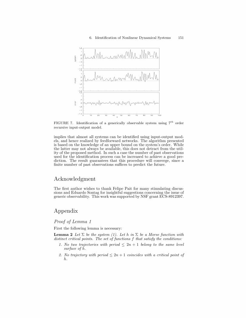
6. Identification of Nonlinear Dynamical Systems 151
FIGURE 7. Identification of a generically observable system using 7th orderrecursive input-output model.
implies that almost all systems can be identified using input-output mod-els, and hence realized by feedforward networks. The algorithm presentedis based on the knowledge of an upper bound on the system’s order. Whilethe latter may not always be available, this does not detract from the util-ity of the proposed method. In such a case the number of past observationsused for the identification process can be increased to achieve a good pre-diction. The result guarantees that this procedure will converge, since afinite number of past observations suffices to predict the future.
Acknowledgment
The first author wishes to thank Felipe Pait for many stimulating discus-sions and Eduardo Sontag for insightful suggestions concerning the issue ofgeneric observability. This work was supported by NSF grant ECS-8912397.
Appendix
Proof of Lemma 1
First the following lemma is necessary:
Lemma 2 Let Σ be the system (1). Let h in Σ be a Morse function withdistinct critical points. The set of functions f that satisfy the conditions:
1. No two trajectories with period ≤ 2n + 1 belong to the same levelsurface of h.
2. No trajectory with period ≤ 2n + 1 coincides with a critical point ofh.

152 A. U. Levin , K. S. Narendra
3. No integral trajectory contains two or more critical points of h.
4. No integral trajectory (except equilibrium points) belongs to a singlelevel surface of h.
is open and dense in C∞.
Proof: The proof of the lemma is an immediate consequence of transversal-ity theory. Violation of any of the above conditions involves the intersectionof manifolds whose sum of dimensions is less then n, i.e., manifolds whichdo not intersect transversally. Since transversal intersections are genericthe conditions follow.
Proof of Lemma 1: Let fi(x)= f(x, ui), where ui denotes the input at
time i. For a given f , Σ will be observable if the mapping φ : ∆(F ×F)×X × X → 2n+1 ×2n+1 defined by
φ(f, f, x, z, u∗) =
h f1(x)h f2 f1(x)...h f2n+1 . . . f1(x)
,
h f1(z)h f2 f1(z)...h f2n+1 . . . f1(z)
(30)
is transversal to W = ∆(2n+1 ×2n+1).To prove that this is true for a generic f , we will consider the fam-
ily of maps F (x, s) = f(x) + sg(x) where s is a parameter and g is asmooth function. In the same manner that φ was defined, we can defineΦ(f, f, x, z, u∗, s) by replacing fi(x) in (30) with Fi(x, s).
Now, from the Transversality Theorem, if Φ∩W then for a generic f ,φ∩W, i.e., the system is observable. By definition, Φ∩W if, for each x = z,either φ(f, f, x, z) ∈ W or ∂Φ
∂s |s=0 spans Wc (the complement of W).Since all elements of W are of the form (w,w), then if we can find g such
that, whenever φ(f, f, x, z) ∈ W, ∂Φ∂s |s=0 is of the form
a1 0 . . . 0∗ a2 . . . 0
...∗ ∗ . . . a2n+1
∣∣∣∣∣∣∣∣∣
b1 0 . . . 0∗ b2 . . . 0
...∗ ∗ . . . b2n+1
(31)
where ai = bi for all i, ∂Φ∂s |s=0 will span Wc and thus φ∩W.
Four possible cases need to be considered:
Case I: Neither x nor z is periodic with period ≤ 2n + 1.
The trajectories of both x and z consist of at least 2n + 1 distinct points.If φ(f, f, x, z) ∈ W, the mapping is transversal, else we need to show that∂Φ∂s |s=0 spans Wc. For 2n + 1, write N .
∂Φ∂s |s=0 = (32)
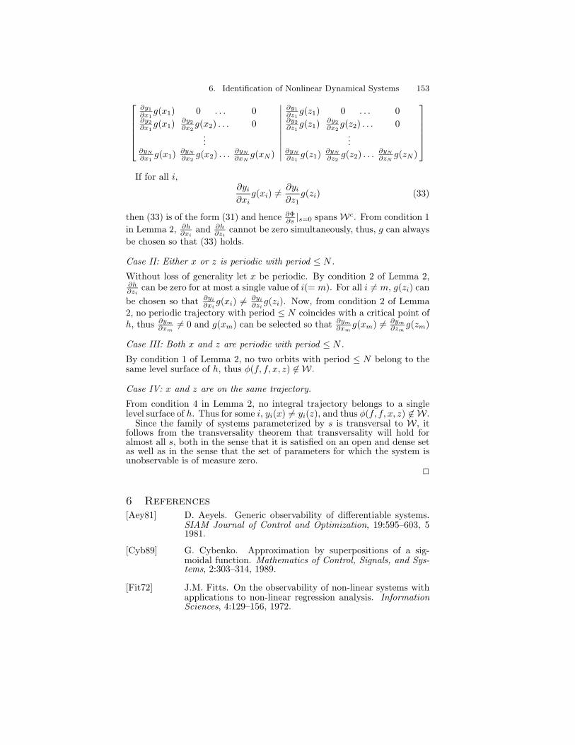
6. Identification of Nonlinear Dynamical Systems 153
∂y1∂x1
g(x1) 0 . . . 0∂y2∂x1
g(x1) ∂y2∂x2
g(x2) . . . 0...
∂yN
∂x1g(x1) ∂yN
∂x2g(x2) . . . ∂yN
∂xNg(xN )
∣∣∣∣∣∣∣∣∣∣
∂y1∂z1
g(z1) 0 . . . 0∂y2∂z1
g(z1) ∂y2∂x2
g(z2) . . . 0...
∂yN
∂z1g(z1) ∂yN
∂z2g(z2) . . . ∂yN
∂zNg(zN )
If for all i,∂yi
∂xig(xi) = ∂yi
∂z1g(zi) (33)
then (33) is of the form (31) and hence ∂Φ∂s |s=0 spans Wc. From condition 1
in Lemma 2, ∂h∂xi
and ∂h∂zi
cannot be zero simultaneously, thus, g can alwaysbe chosen so that (33) holds.
Case II: Either x or z is periodic with period ≤ N .
Without loss of generality let x be periodic. By condition 2 of Lemma 2,∂h∂zi
can be zero for at most a single value of i(= m). For all i = m, g(zi) canbe chosen so that ∂yi
∂xig(xi) = ∂yi
∂zig(zi). Now, from condition 2 of Lemma
2, no periodic trajectory with period ≤ N coincides with a critical point ofh, thus ∂ym
∂xm= 0 and g(xm) can be selected so that ∂ym
∂xmg(xm) = ∂ym
∂zmg(zm)
Case III: Both x and z are periodic with period ≤ N .
By condition 1 of Lemma 2, no two orbits with period ≤ N belong to thesame level surface of h, thus φ(f, f, x, z) ∈ W.
Case IV: x and z are on the same trajectory.
From condition 4 in Lemma 2, no integral trajectory belongs to a singlelevel surface of h. Thus for some i, yi(x) = yi(z), and thus φ(f, f, x, z) ∈ W.
Since the family of systems parameterized by s is transversal to W, itfollows from the transversality theorem that transversality will hold foralmost all s, both in the sense that it is satisfied on an open and dense setas well as in the sense that the set of parameters for which the system isunobservable is of measure zero.
6 References[Aey81] D. Aeyels. Generic observability of differentiable systems.
SIAM Journal of Control and Optimization, 19:595–603, 51981.
[Cyb89] G. Cybenko. Approximation by superpositions of a sig-moidal function. Mathematics of Control, Signals, and Sys-tems, 2:303–314, 1989.
[Fit72] J.M. Fitts. On the observability of non-linear systems withapplications to non-linear regression analysis. InformationSciences, 4:129–156, 1972.

154 A. U. Levin , K. S. Narendra
[GG73] M. Golubitsky and V. Guillemin. Stable Mappings and TheirSingularities. Springer-Verlag, 1973.
[GP74] V. Guillemin and A. Pollack. Differential Topology.Prentice-Hall, 1974.
[HSW89] K. Hornik, M. Stinchcombe, and H. White. Multilayer feed-forward networks are universal approximators. Neural Net-works, 2:359–366, 1989.
[JC73] J.B. Cruz, Jr., editor. System Sensitivity Analysis. Dowsen,Hutchinson and Ross Inc., 1973.
[Jor86] M.I. Jordan. Attractor dynamics and parallelism in a con-nectionist sequential machine. In Proceedings of the EighthAnnual Conference of the Cognitive Science Society, pages531–546, Amherst 1986, 1986. Lawrence Erlbaum, Hillsdale.
[JS90] B. Jakubczyk and E.D. Sontag. Controllability of nonlin-ear discrete-time systems: A lie algebraic approach. SIAMJournal of Control and Optimization, 28:1–33, January 1990.
[LB85] I.J. Leontaritis and S.A. Billings. Input-output parametricmodels for non-linear systems, part i: Deterministic nonlin-ear systems. International Journal of Control, 41:303–328,1985.
[Lev92] A.U. Levin. Neural Networks in Dynamical Systems: a Sys-tem Theoretic Approach. Ph.D. thesis, Yale University, NewHaven, CT, November 1992.
[Lju77] L. Ljung. Analysis of recursive stochastic algorithms. IEEETransactions on Automatic Control, 22:551–575, 1977.
[L.L91] L.Ljung. Issues in system identification. IEEE Control Sys-tems Magazine, 11:25–29, 1991.
[LN93] A.U. Levin and K.S. Narendra. Control of non-linear dynam-ical systems using neural networks. controllability and stabi-lization. IEEE Transactions on Neural Networks, 4:192–206,March 1993.
[LN96] A.U. Levin and K.S. Narendra. Control of non-linear dy-namical systems using neural networks – part ii: Observabil-ity, identification and control. IEEE Transactions on NeuralNetworks, 7:30–42, January 1996.
[MRtPRG86] J.L. McClelland, D.E. Rumelhart, and the PDP Re-search Group. Parallel Distributed Processing: Explorationsin the Microstructure of Cognition, volume 2. MIT Press,Cambridge, 1986.
[NP90] K.S. Narendra and K. Parthasarathy. Identification andcontrol of dynamical systems using neural networks. IEEETransactions on Neural Networks, 1:4–27, March 1990.
6. Identification of Nonlinear Dynamical Systems 155
[NP91] K.S. Narendra and K. Parthasarathy. Gradient methods forthe optimization of dynamical systems containing neural net-works. IEEE Transactions on Neural Networks, 2:252–261,March 1991.
[RS80] M. Reed and B. Simon. Methods of Modern MathematicalPhysics I: Functional Analysis. Academic Press, 1980.
[Rug81] W.J. Rugh. Nonlinear System Theory: the Volterra/WienerApproach. The John Hopkins University Press, 1981.
[Son79a] E.D. Sontag. On the observability of polynomial systems, i:Finite time problems. SIAM Journal of Control and Opti-mization, 17:139–150, 1979.
[Son79b] E.D. Sontag. Polynomial Response Maps. Springer-Verlag,1979.
[WZ89] R.J. Williams and D. Zipser. A learning algorithm for con-tinually running fully recurrent neural networks. NeuralComputation, 1:270–280, 1989.

156 A. U. Levin , K. S. Narendra

7
Neural Network Control ofRobot Arms and NonlinearSystems
F.L. LewisS. JagannathanA. Yesildirek
ABSTRACT Neural network (NN) controllers are designed that give guar-anteed closed-loop performance in terms of small tracking errors and bound-ed controls. Applications are given to rigid-link robot arms and a class ofnonlinear systems. Both continuous-time and discrete-time NN tuning al-gorithms are given. New NN properties such as strict passivity avoid theneed for persistence of excitation. New NN controller structures avoid theneed for preliminary off-line learning, so that the NN weights are easilyinitialized and the NN learns on-line in real-time. No regression matrixneed be found, in contrast to adaptive control. No certainty equivalenceassumption is needed, as Lyapunov proofs guarantee simultaneously thatboth tracking errors and weight estimation errors are bounded.
1 Introduction
Neural networks (NN) can be used for classification and decision-making,or for controls applications. Some background on NN is given in [MSW91,MB92, Pao89, PG89, RHW86, Wer74, Wer89]. In classification and decis-ion-making NN have by now achieved common usage and are very effectivein solving certain types of problems, so that their use is commonplace inimage and signal processing and elsewhere. A major reason for this isthe existence of a mathematical framework for selecting the NN weightsusing proofs based on the notion of energy function, or of algorithms thateffectively tune the weights on line.
1.1 Neural Networks for Control
In controls there have been many applications of NN, but few rigorousjustifications or guarantees of performance. The use of ad hoc controllerstructures and tuning strategies has resulted in uncertainty on how to se-lect the initial NN weights, so that a so-called ’learning phase’ is oftenneeded that can last up to 50,000 iterations. Although preliminary NN off-

158 F.L. Lewis, S. Jagannathan, A. Yesildirek
line training may appear to have a mystique due to its anthropomorphicconnotations, it is not a suitable strategy for controls purposes.
There are two sorts of controls applications for NN: identification andcontrol. Some background on robotics and controls applications of NNis given in [CS92, CS93, HHA92, IST91, MSW91, Nar91, NA87, NP90,YY92]. In identification the problems associated with implementation areeasier to solve and there has been good success (see references). Since thesystem being identified is usually stable, it is only necessary to guaranteethat the weights remain bounded. This can generally be accomplishedusing standard tuning techniques such as the delta rule with, for instance,backpropagation of error. In identification, it is generally not a problem tohave a learning phase.
Unfortunately, in closed-loop control using NN the issues are very muchmore complicated, so that approaches that are suitable for NN classifica-tion applications are of questionable use. A long learning phase is detri-mental to closed-loop applications. Uncertainty on how to initialize theNN weights to give initial stability means that during the learning phasethe NN controller cannot be switched on line. Most importantly, in closed-loop control applications one must guarantee two things— boundednessof the NN weights and boundedness of the regulation or tracking errors,with the latter being the prime concern of the engineer. This is diffi-cult using approaches to NN that are suitable for classification applica-tions. Some work that successfully uses NN rigorously for control appearsin [CK92, LC93, PI91, PI92, RC95, Sad91, SS91], though most of thesepapers that contain proofs are for 2-layer (linear-in-the-parameters) NN.
The background work for this chapter appears in [JL96, LLY95, LYL96,YL95]. To guarantee performance and stability in closed-loop control ap-plications using multilayer (nonlinear) NN, it is found herein that the stan-dard delta rule does not suffice. Indeed, we see that the tuning rules mustbe modified with extra terms. In this chapter we give new controller struc-tures that make it easy to initialize the NN weights and still guaranteestability. No off-line learning phase is needed, and tuning to small errorsoccurs in real-time in fractions of a second. New NN properties such as pas-sivity and robustness make the controller robust to unmodeled dynamicsand bounded disturbances.
Our primary application is NN for control of rigid robot manipulators,though a section on nonlinear system control shows how the technique canbe generalized to other classes of systems in a straightforward manner. Ourwork provides continuous-time update algorithms for the NN weights; a sec-tion is added to show how to use the same approach to derive discrete-timeweight tuning algorithms, which are directly applicable in digital control.
1.2 Relation to Adaptive Control
One will notice, of course, the close connection between NN control andadaptive control [Cra88, Goo91, KC91, SB89]; in fact, from this chapterone may infer that NN comprise a special class of nonlinear adaptive con-trollers with very important properties. Thus, this chapter considerablyextends the capabilities of linear-in-the-parameters adaptive control. Inindirect adaptive control, especially in discrete time, one makes a certaintyequivalence assumption that allows one to decouple the controller designfrom the adaptive identification phase. This is akin to current approaches

7. Neural Network Control of Robot Arms 159
to NN control. This chapter shows how to perform direct NN control, evenin the discrete-time case, so that the certainty equivalence assumption isnot needed. The importance of this is that closed-loop performance interms of small tracking errors and bounded controls is guaranteed.
In adaptive control it is often necessary to make assumptions, like those ofErzberger or the model-matching conditions, on approximation capabilitiesof the system, which may not hold. By contrast the NN approximationcapabilities employed in this chapter always hold. In the NN controllersof this chapter, no persistence of excitation condition is needed. Finally, amajor debility of adaptive control is the need to find a ’regression matrix’,which often entails determining the full dynamics of the system. In NNcontrol, no regression matrix is needed; the NN learns in real time thedynamical structure of the unknown system.
2 Background in Neural Networks, Stability, andPassivity
Some fairly standard notation is needed prior to beginning. Let IR denotethe real numbers, IRn denote the real n-vectors, IRm×n the real m × nmatrices. Let S be a compact simply connected set of IRn. With mapf : S → IRm, define Cm(S) as the space such that f is continuous. Wedenote by ‖.‖ any suitable vector norm; when it is required to be specificwe denote the p-norm by ‖.‖p. The supremum norm of f(x) (over S) isdefined as [Bar64]
supx∈S
‖f(x)‖, f : S → IRm.
Given A = [aij ], B ∈ IRm×n the Frobenius norm is defined by
‖A‖2F = tr(AT A) =
∑i,j
a2ij
with tr() the trace. The associated inner product is < A,B >F = tr(AT B).The Frobenius norm is nothing but the vector 2-norm over the space definedby stacking the matrix columns into a vector. As such, it cannot be definedas the induced matrix norm for any vector norm, but is compatible withthe 2-norm so that ‖Ax‖2 ≤ ‖A‖F ‖x‖2, with A ∈ IRm×n and x ∈ IRn.
When x(t) ∈ IRn is a function of time we may refer to the standard Lp
norms [LAD93] denoted ‖x(.)‖p. We say vector x(t) is bounded if the L∞norm is bounded. We say matrix A(t) ∈ IRm×n is bounded if its inducedmatrix ∞-norm is bounded.
2.1 Neural Networks
Given x= [x1 x2 ...xN1]T ∈ IRN1 , a three-layer neural net (NN) (Figure 1)has a net output given by
yi =N2∑j=1
wijσ[N1∑k=1
vjkxk + θvj ] + θwi]; i = 1, .., N3 (1)
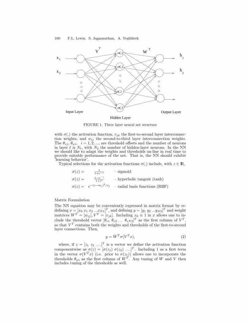
160 F.L. Lewis, S. Jagannathan, A. Yesildirek
h
Output Layer
V W
Hidden Layer
Input Layer
σ(.)
σ(.)
σ(.)
σ(.)
T T
x
x
1
2 2
1h
FIGURE 1. Three layer neural net structure
with σ(.) the activation function, vjk the first-to-second layer interconnec-tion weights, and wij the second-to-third layer interconnection weights.The θvj , θwi, i = 1, 2, ..., are threshold offsets and the number of neuronsin layer is N, with N2 the number of hidden-layer neurons. In the NNwe should like to adapt the weights and thresholds on-line in real time toprovide suitable performance of the net. That is, the NN should exhibit’learning behavior’.
Typical selections for the activation functions σ(.) include, with z ∈ IR,
σ(z) = 11+e−z – sigmoid
σ(z) = 1−e−z
1+ez – hyperbolic tangent (tanh)
σ(z) = e−(z−mj)2/sj – radial basis functions (RBF)
Matrix FormulationThe NN equation may be conveniently expressed in matrix format by re-defining x = [x0 x1 x2 ...xN1]T , and defining y = [y1 y2 ...yN3]T and weightmatrices WT = [wij ], V T = [vjk]. Including x0 ≡ 1 in x allows one to in-clude the threshold vector [θv1 θv2 . . . θvN2]T as the first column of V T ,so that V T contains both the weights and thresholds of the first-to-secondlayer connections. Then,
y = WT σ(V T x), (2)
where, if z = [z1 z2 . . .]T is a vector we define the activation functioncomponentwise as σ(z) = [σ(z1) σ(z2) . . .]T . Including 1 as a first termin the vector σ(V T x) (i.e. prior to σ(z1)) allows one to incorporate thethresholds θwi as the first column of WT . Any tuning of W and V thenincludes tuning of the thresholds as well.

7. Neural Network Control of Robot Arms 161
Although, to account for nonzero thresholds, the vector x may be aug-mented by x0 = 1 and the vector σ(V T x) by the constant first entry of 1,we loosely say that x ∈ IRN1 and σ : IRN2 → IRN2.
Approximation Property of NN
With x ∈ IRn, A general function f(x) ∈ Cm(S) can be written as
f(x) = WT σ(V T x) + ε(x), (3)
with N1 = n, N3 = m, and ε(x) a NN functional reconstruction errorvector. If there exist N2 and constant ’ideal’ weights W and V so thatε = 0 for all x ∈ S, we say f(x) is in the functional range of the NN. Ingeneral, given a real number εN > 0, we say f(x) is within εN of the NNrange if there exist N2 and constant weights so that for all x ∈ IRn, (3)holds with ‖ε‖ < εN . Unless the net is “minimal“, the weights minimizingmay not be unique [AS92, Sus92].
Various well-known results for various activation functions σ(.), based,e.g. on the Stone-Weierstrass theorem, say that any sufficiently smoothfunction can be approximated by a suitably large net [Cyb89, HSW89,PS91, SS91]. The functional range of NN 2 is said to be dense in Cm(S) iffor any f ∈ Cm(S) and εN > 0 there exist finite N2, and W and V suchthat (3) holds with ε < εN , N1 = n,N3 = m. Typical results are likethe following, for the case of σ(.) any “squashing function” (a bounded,measurable, nondecreasing function from the real numbers onto (0, 1)), forinstance the sigmoid function.
Theorem 2.6 Set N1 = n, N3 = m and let σ(.) be any squashing function.Then the functional range of NN (2) is dense in Cm(S).
In this result, the metric defining denseness is the supremum norm.Moreover, the last layer thresholds θwi are not needed for this result. Theengineering design issues of selecting σ(.), and of choosing N2 for a specifiedS ⊂ IRn and εN are current topics of research (see e.g. [PS91]).
2.2 Stability and Passivity of Dynamical Systems
Some stability notions are needed to proceed [LAD93]. Consider the non-linear system
x = f(x, u, t), y = h(x, t).(2.4) (4)
We say the solution is uniformly ultimately bounded (UUB) if there existsa compact set U ⊂ IRn such that for all x(t0) = x0 ∈ U, there exists anε > 0 and a number T (ε, x0) such that x(t) < ε for all t ≥ t0 + T . UUBis a notion of stability in a practical sense that is good enough for suitabletracking performance of robot manipulators if, of course, the bound is smallenough.
Passive systems are important in robust control, where bounded distur-bances or unmodeled dynamics are present. Since we intend to define somenew passivity properties of NN, some aspects of passivity will subsequentlybe important [GS84, Lan79, LAD93, SL91]. A system with input u(t) and

162 F.L. Lewis, S. Jagannathan, A. Yesildirek
output y(t) is said to be passive if it verifies an equality of the so-called’power form’
L(t) = yT u − g(t) (5)
with L(t) lower bounded and g(t) ≥ 0. That is,
∫ T
0
yT (τ)u(t) dτ ≥∫ T
0
g(t) dt − γ2 (6)
for all T ≥ 0 and some γ ≥ 0.We say the system is dissipative if it is passive and in addition∫ ∞
o
yT (τ)u(τ) dt = 0 implies∫ ∞
o
g(τ) dτ > 0 (7)
A special sort of dissipativity occurs if g(t) is a monic quadratic functionof x with bounded coefficients, where x(t) is the internal state of the system.We call this state strict passivity, and are not aware of its use previouslyin the literature (although cf. [GS84]). Then the L2 norm of the stateis bounded above in terms of the L2 inner product of output and input(i.e. the power delivered to the system). This we use to advantage toconclude some internal boundedness properties of the system without theusual assumptions of observability (e.g. persistence of excitation), stability,etc.
3 Dynamics of Rigid Robot Arms
In some sense the application of NN controllers to rigid robot arms turns outto be very natural. A main reason is that the robot dynamics satisfy someimportant properties, including passivity, that are very easy to preserve inclosed loop by considering the corresponding properties on the NN. Thus,one is motivated in robotics applications to discover new properties of NN.The dynamics of robot manipulators and some of their properties are nowdiscussed.
3.1 Robot Dynamics and Properties
The dynamics of an n-link rigid (i.e. no flexible links or joints) robotmanipulator may be expressed in the Lagrange form [Cra88, LAD93]
M(q)q + Vm(q, q)q + G(q) + F (q) + td = t (8)
with q(t) ∈ IRn the joint variable vector, M(q) the inertia matrix, Vm(q, q)the Coriolis/centripetal matrix, G(q) the gravity vector, andF (q) the fric-tion. Bounded unknown disturbances (including e.g. unstructured unmod-eled dynamics) are denoted by td, and the control input torque is τ(t).
The following standard properties of the robot dynamics are required[LAD93].
Property 1: M(q) is a positive definite symmetric matrix bounded bym1I ≤ M(q) ≤ m2I with m1, m2 known positive constants.
Property 2: Vm(q, q) is bounded by vb(q)‖q‖, with vb(q) ∈ C1(S).

7. Neural Network Control of Robot Arms 163
Property 3: The matrix M − 2Vm is skew-symmetric.Property 4: The unknown disturbance satisfies ‖τd‖ < bd, with bd a
known positive constant.
3.2 Tracking a Desired Trajectory and the Error Dynamics
An important application in robot arm control is for the manipulator tofollow a prescribed trajectory.
Error Dynamics
Given a desired arm trajectory qd(t)IRn the tracking error is
e(t) = qd(t) − q(t). (9)
It is typical in robotics to define a so-called filtered tracking error as
r = e + Λe (10)
where Λ = ΛT > 0 is a design parameter matrix, usually selected diagonal.Differentiating r(t) and using (8), the arm dynamics may be written interms of the filtered tracking error as
Mr = −Vmr − τ + f + τd (11)
where the important nonlinear robot function is
f(x) = M(q)(qd + e) + Vm(q, q)(qd + e) + G(q) + F (q.) (12)
and we may define, for instance,
x ≡ [eT eT qTd qT
d qTd ]T . (13)
A suitable control input for trajectory following is given by
τo = f + Kvr (14)
Kv = KTv > 0 a gain matrix and f(x) an estimate of f(x) found by
some means not yet discussed. Using this control, the closed-loop systembecomes
Mr = −(Kv + Vm)r + f + τd ≡ −(Kv + Vm)r + ζo (15)
where the functional estimation error is given by
f = f − f (16)
This is an error system wherein the filtered tracking error is driven by thefunctional estimation error. The control τ0 incorporates a proportional-plus-derivative (PD) term in Kvr = Kv(e + Λe).

164 F.L. Lewis, S. Jagannathan, A. Yesildirek
The Control ProblemIn the remainder of the chapter we shall use (15) to focus on selecting NNtuning algorithms that guarantee the stability of the filtered tracking errorr(t). Then, since (10),with the input considered as r(t) and the output ase(t) describes a stable system, standard techniques [LL92, SL91] guaranteethat e(t) exhibits stable behavior. In fact, one may show using the notionof ’operator gain’ that ‖e‖2 ≤ ‖r‖2/σmin(Λ), ‖e‖2 ≤ ‖r‖2, with σmin(Λ)the minimum singular value of Λ. Generally Λ is diagonal, so that σmin(Λ)is the smallest element of Λ.
Therefore, the control design problem is to complete the definition of thecontroller so that both the error r(t) and the control signals are bounded.It is important to note that the latter conclusion hinges on showing thatthe estimate f(x) is bounded. Moreover, for good performance, the boundson r(t) should be in some sense ’small enough’.
Passivity Property
The next property is important in the design of robust NN controllers.Property 5: The dynamics (15) from ζo(t) to r(t) are a state strict
passive system.Proof of Property 5:
Take the nonnegative function
L =12rT Mr
so that, using (15)
L = rT Mr + 12rT Mr = −rT Kvr + rT (M − 2Vm)r + rT ζo
whence skew-symmetry yields the power form
L = rT ζo − rT Kvr.
4 NN Controller for Robot Arms
In this section we derive a NN controller for the robot dynamics in Section 3.This controller consists of the control strategy ( developed in that section,where the robot function estimate f(x) is now provided by a NN. Since wemust demonstrate boundedness of both the NN weights and the trackingerror, it will be found that the standard delta rule does not suffice in tuningthis NN, but extra terms must be added.
4.1 Some Assumptions and Facts
Some required mild assumptions are now stated. The assumptions will betrue in every practical situation, and are standard in the existing literature.

7. Neural Network Control of Robot Arms 165
Assumption 1 The nonlinear robot function (12) is given by a neuralnet as in (3)for some constant ’target’ NN weights W and V , where thenet reconstruction error ε(x) is bounded by a known constant εN .
Unless the net is “minimal“, suitable target weights may not be unique[AS92, Sus92]. The ’best’ weights may then be defined as those which mini-mize the supremum norm over S of ε(x). This issue is not of major concernhere, as we only need to know that such target weights exist; their actualvalues are not required. According to the discussion in Section 2, results onthe approximation properties of NN guarantee that this assumption doesin fact hold. This is in direct contrast to the situation often arising inadaptive control, where assumptions (e.g. Erzberger, model-matching) onthe plant structure often do not hold in practical applications.
For notational convenience define the matrix of all the weights as
Z =[
W 00 V
](17)
Assumption 2The target weights are bounded by known positive values so that ‖V ‖F ≤
VM , ‖W‖F ≤ WM , or‖Z‖F ≤ ZM (18)
with ZM known.Assumption 3The desired trajectory is bounded in the sense, for instance, that∥∥∥∥∥∥
qd
qd
q
∥∥∥∥∥∥ ≤ Qd, (19)
where Qd ∈ IR is a known constant.The next fact follows directly from the assumptions and previous defini-
tions.Fact 4For each time t, x(t) in (13) is bounded by
‖x‖ ≤ c1Qd + c2‖r‖ (20)
for computable positive constants ci (c2 decreases as Λ increases.)
4.2 A Property of the Hidden-Layer Output Error
The next discussion is of major importance in this paper (cf. [PI92]). Itshows a key structural property of the hidden-layer output error that playsa major role in the upcoming closed-loop stability proof. It is in effect thestep that allows one to progress to nonlinear adaptive control as opposed tolinear-in-the-parameters control. The analysis introduces some novel termsthat will appear directly in the NN weight tuning algorithms, effectivelyadding additional terms to the standard delta rule weight updates.
With V , W some estimates of the target weight values, define the weightdeviations or weight estimation errors as
V = V − V , W = W − W , Z = Z − Z. (21)

166 F.L. Lewis, S. Jagannathan, A. Yesildirek
In applications, the weight estimates are provided by the NN weighttuning rules. Define the hidden-layer output error for a given x as
σ = σ − σ ≡ σ(V T x) − σ(V T x). (22)
The Taylor series expansion for a given x may be written as
σ(V T x) = σ(V T x) + σ′(V T x)V T x + O(V T x)2 (23)
with
σ′(z) ≡ dσ(z)dz
|z=z,
and O(z)2 denoting terms of order two. Denoting σ′ = σ′(V T x), we have
σ = σ′(V T x)V T x + O(V T x)2 = σ′V T x + O(V T x)2. (24)
Different bounds may be put on the Taylor series higher-order termsdepending on the choice for σ(.). Noting that
O(V T x)2 = [σ(V T x) − σ(V T x)] − σ′(V T x)V T x
we take the following.Fact 5For sigmoid, RBF, and tanh activation functions, the higher-order termsin the Taylor series are bounded by
‖O(V T x)2‖ ≤ c3 + c4Qd‖V ‖F + c5‖V ‖F ‖r‖where ci are computable positive constants.
Fact 5 is direct to show using (20),some standard norm inequalities, andthe fact that σ(.) and its derivative are bounded by constants for RBF,sigmoid, and tanh.
The extension of these ideas to nets with greater than three layers is notdifficult, and leads to composite function terms in the Taylor series (givingrise to backpropagation filtered error terms for the multilayer net case– SeeTheorem4.6.
4.3 Controller Structure and Error System Dynamics
The NN controller structure will now be defined; it appears in Figure 2,where q ≡ [qT qT ]T , , e ≡ [eT eT ]T . It is important that the NN controllerstructure is not ad hoc, but follows directly from a proper treatment of therobot error dynamics and its properties; it is not open to question.
NN ControllerDefine the NN functional estimate of (12) by
f(x) = WT σ(V T x), (25)
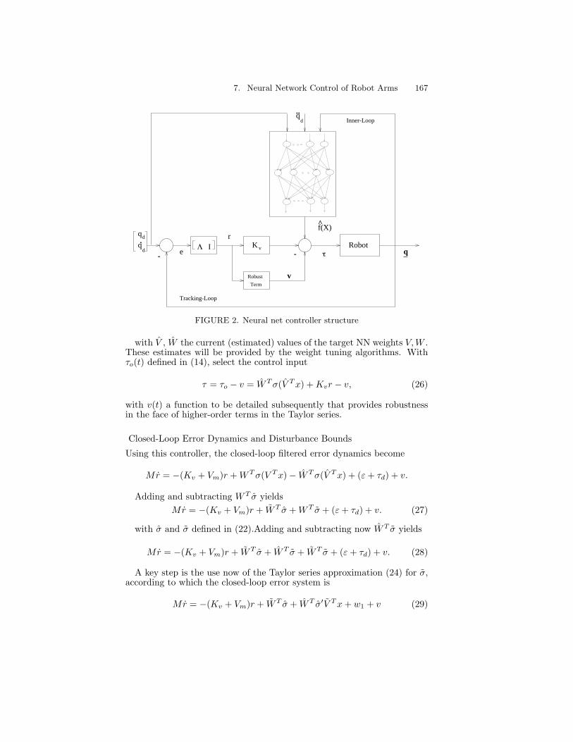
7. Neural Network Control of Robot Arms 167
Iqr
K Robot
f(X)
q
Inner-Loop
Tracking-Loop
q
d
d
v
Robust
Term
e τ
..
.
^
--
v
d
q
_Λ
FIGURE 2. Neural net controller structure
with V , W the current (estimated) values of the target NN weights V,W .These estimates will be provided by the weight tuning algorithms. Withτo(t) defined in (14), select the control input
τ = τo − v = WT σ(V T x) + Kvr − v, (26)
with v(t) a function to be detailed subsequently that provides robustnessin the face of higher-order terms in the Taylor series.
Closed-Loop Error Dynamics and Disturbance Bounds
Using this controller, the closed-loop filtered error dynamics become
Mr = −(Kv + Vm)r + WT σ(V T x) − WT σ(V T x) + (ε + τd) + v.
Adding and subtracting WT σ yieldsMr = −(Kv + Vm)r + WT σ + WT σ + (ε + τd) + v. (27)
with σ and σ defined in (22).Adding and subtracting now WT σ yields
Mr = −(Kv + Vm)r + WT σ + WT σ + WT σ + (ε + τd) + v. (28)
A key step is the use now of the Taylor series approximation (24) for σ,according to which the closed-loop error system is
Mr = −(Kv + Vm)r + WT σ + WT σ′V T x + w1 + v (29)

168 F.L. Lewis, S. Jagannathan, A. Yesildirek
where the disturbance terms are
w1(t) = WT σ′V T x + WT O(V T x)2 + (ε + τd). (30)
Unfortunately, using this error system does not yield a compact set outsidewhich a certain Lyapunov function derivative is negative; this makes theupcoming stability proof extremely difficult. Therefore, write finally theerror system
Mr = −(Kv + Vm)r + WT (σ − σ′V T x) + WT σ′V T x + w + v
≡ −(Kv + Vm)r + ζ1. (31)
where the disturbance terms arew(t) = WT σ′V T x + WT O(V T x)2 + (ε + τd). (32)
It is important to note that the NN reconstruction error ε(x), the robotdisturbances τd, and the higher-order terms in the Taylor series expansionof f(x) all have exactly the same influence as disturbances in the error sys-tem. The next key bound is required. Its importance is in allowing one tobound the unknown disturbance w(t) at each time by a known computablefunction; it follows from Fact 5 and some standard norm inequalities.
Fact 6The disturbance term (32) is bounded according to
‖w(t)‖ ≤ (εN + bd + c3ZM ) + c6ZM‖Z‖F + c7ZM‖Z‖F ror
w(t) ≤ C0 + C1‖Z‖F + C2‖Z‖F ‖r‖ (33)
with Ci known positive constants.
4.4 NN Weight Updates for Guaranteed TrackingPerformance
We give here a NN weight tuning algorithm that guarantees the perfor-mance of the closed-loop system. To confront the stability and trackingperformance of the closed-loop NN robot arm controller we require: (1)the modification of the delta rule weight tuning algorithm, and (2) the ad-dition of a robustifying term v(t). The problem in the closed-loop controlcase is that, though it is not difficult to conclude that the error r(t) isbounded, it is very hard without these modifications to show that the NNweights are bounded in general. Boundedness of the weights is needed toverify that the control input τ(t) remains bounded.
The next main theorem relies on an extension to Lyapunov theory. Thedisturbance τd, the NN reconstruction error ε , and the nonlinearity of f(x)make it impossible to show that the Lyapunov derivative L is nonpositivefor all r(t) and weight values. In fact, it is only possible to show that L isnegative outside a compact set in the state space. This, however, allows oneto conclude boundedness of the tracking error and the neural net weights.In fact, explicit bounds are discovered during the proof.
7. Neural Network Control of Robot Arms 169
Theorem 4.6 Let the desired trajectory be bounded by (19). Take thecontrol input for the robot (8) as (26) with robustifying term
v(t) = −KZ(‖Z‖F + ZM )r (34)
and gainKZ > C2 (35)
with C2 the known constant in (33). Let NN weight tuning be provided by
˙W = F σrT − F σ′V T xrT − κF‖r‖W (36)˙V = Gx(σ′T W r)T − κG‖r‖V (37)
with any constant matrices F = FT > 0, G = GT > 0, and scalar designparameter κ > 0 . Then, for large enough control gain Kv, the filteredtracking error r(t) and NN weight estimates V , W are UUB, with practicalbounds given specifically by the right-hand sides of (39) and (40). Moreover,the tracking error may be kept as small as desired by increasing the gainsKv in (26).
Proof: Let the approximation property (3) hold for f(x) in (12) with agiven accuracy εN for all x in the compact set Ux ≡ x|‖x‖ ≤ bx withbx > c1Qd in (20). Define Ur = r|‖r‖ ≤ (bx − c1Qd)/c2. Let r(0) ∈ Ur.Then the approximation property holds.
Define the Lyapunov function candidate
L = rT Mr + tr(WT F−1W ) + tr(V T G−1V ). (38)
Differentiating yields
L =12rT Mr + rT Mr + tr(WT F−1 ˙W ) + tr(V T G−1 ˙V ).
Substituting now from the error system (31) yields
L = −rT Kvr +12rT (M − 2Vm)r + trWT (F−1 ˙W + σrT − σ′V T xrT )
+trV T (G−1 ˙V + xrT WT σ′) + rT (w + v).
The tuning rules give
L = −rT Kvr + κ‖r‖trWT (W − W ) + κ‖r‖trV T (V − V ) + rT (w + v)
= −rT Kvr + κ‖r‖trZT (Z − Z) + rT (w + v).
Since
trZT (Z − Z) =< Z, Z >F −‖Z‖2F ≤ ‖Z‖F ‖Z‖F − ‖Z‖2
F ,

170 F.L. Lewis, S. Jagannathan, A. Yesildirek
there results
L ≤ −Kvmin‖r‖2 + κ‖r‖‖Z‖F (ZM − ‖Z‖F ) − KZ(‖Z‖F + ZM )‖r‖2
+‖r‖ ‖w‖≤ −Kvmin‖r‖2 + κ‖r‖‖Z‖F (ZM − ‖Z‖F ) − KZ(‖Z‖F + ZM )‖r‖2
+‖r‖[C0 + C1‖Z‖F + C2‖Z‖F ‖r‖]≤ −‖r‖[Kvmin‖r‖ + κ‖Z‖F (‖Z‖F − ZM ) − C0 − C1‖Z‖F ],
where Kvmin is the minimum singular value of Kv and the last inequalityholds due to (35). Thus, L is negative as long as the term in braces ispositive. We show next that this occurs outside a compact set in the(‖r‖, ‖Z‖F ) plane.
Defining C3 = ZM + C1/κ and completing the square yields
Kvmin‖r‖ + κ‖Z‖F (‖Z‖F − C3) − C0
= κ(‖Z‖F − C3/2)2 − κC23/4 + Kvmin‖r‖ − C0,
which is guaranteed positive as long as either
‖r‖ >κC2
3/4 + C0
Kvmin≡ br (39)
or‖Z‖F > C3/2 +
√C2
3/4 + C0/κ ≡ bZ , (40)
whereC3 = ZM + C1/κ. (41)
Thus, L is negative outside a compact set. The form of the right-handside of (39) shows that the control gain Kv can be selected large enoughso that br < (bx − c1Qd)/c2. Then, any trajectory r(t) beginning in Ur
evolves completely within Ur. According to a standard Lyapunov theoremextension [LAD93, NA87], this demonstrates the UUB of both ‖r‖ and‖Z‖F .
The complete NN controller is given in Table 1 and illustrated in Figure 2.It is important to note that this is a novel control structure with an innerNN loop and an outer robust tracking loop that has important ramificationsas delineated below. Some discussion of these results is now given.
Bounded Errors and ControlsThe dynamical behavior induced by this controller is as follows. Due tothe presence of the disturbance terms, it is not possible to use Lyapunov’stheorem directly as it cannot be demonstrated that L is always negative;instead an extension to Lyapunov’s theorem is used (cf. [NA87] and The-orem 1.5-6 in [LAD93]). In this extension, it is shown that L is negativeif either ‖r‖ or ‖Z‖ are above some specific bounds. Therefore, if eithernorm increases too much, L decreases so that both norms decrease as well.

7. Neural Network Control of Robot Arms 171
If both norms are small, nothing may be said about L except that it isprobably positive, so that L increases. This has the effect of making theboundary of a compact set an attractive region for the closed-loop system.Thus the errors are guaranteed bounded, but in all probability nonzero.
In applications, therefore, the right-hand sides of (39) and (40) may betaken as practical bounds on the norms of the error r(t) and the weighterrors Z(t). Since the target weights Z are bounded, it follows that theNN weights W (t) and V (t) provided by the tuning algorithms are bounded;hence the control input is bounded.
In fact, it is important to note that according to (39), arbitrarily smalltracking error bounds may be achieved by selecting large control gains Kv.(If Kv is taken as a diagonal matrix, Kvmin is simply the smallest gainelement.) On the other hand, (40) reveals that the NN weight errors arefundamentally bounded by ZM (through C3). The parameter κ offers adesign tradeoff between the relative eventual magnitudes of ‖r‖ and ‖Z‖.
An alternative to guaranteeing the boundedness of the NN weights forthe 2-layer case V = I (i.e. linear in the parameters) is presented in[PI91, RC95] where a projection algorithm is used for tuning W .
Initializing the NN Weights and Real-Time Learning
Note that the problem of net weight initialization occurring in other ap-proaches in the literature does not arise. In fact, selecting the initial weightsW (0), V (0) as zero takes the NN out of the circuit and leaves only the outertracking loop in Figure 2. It is well known that the PD term Kvr in (44)can then stabilize the robot arm on an interim basis until the NN beginsto learn. A formal proof reveals that Kv should be large enough and theinitial filtered error r(0) small enough. The exact value of Kv needed forinitial stabilization is given in [DQLD90], though for practical purposes itis only necessary to select Kv large.
This means that there is no off-line learning phase for this NN controller.Results in a simulation example soon to be presented show that convergenceof the tracking error occurs in real time in a fraction of a second.
Extension of Delta Rule with Error Backpropagation
The first terms of (46), (47) are nothing but continuous-time versions ofthe standard backpropagation algorithm. In fact, the first terms are
˙W = F σrT (42)
V = Gx(σ′T W r)T (43)
In the scalar sigmoid case, for instance
σ′(z) = σ(z)(1 − σ(z)).
so thatσ′T W r = diagσ(V T x)[I − diagσ(V T x)]W r,
which is the filtered error weighted by the current estimate W and mul-tiplied by the usual product involving the hidden-layer outputs.

172 F.L. Lewis, S. Jagannathan, A. Yesildirek
l
q1
1
2
q1
1
2
q2
l
FIGURE 3. 2-link planar elbow arm
The last terms in (46), (47) correspond to the e-modification [NA87]in standard use in adaptive control to guarantee bounded parameter esti-mates. They are needed due to the presence of the NN reconstruction errorε and the robot unmodeled disturbances τd(t).
The second term in (46) is a novel one and bears discussion. The standardbackprop terms can be thought of as backward propagating signals in anonlinear ’backprop’ network [NP90] that contains multipliers. The secondterm in (46) corresponds to a forward traveling wave in the backprop netthat provides a second-order correction to the weight tuning for W . Thisterm is needed to bound certain of the higher-order terms in the Taylorseries expansion of σ, and arises from the extension of adaptive controlfrom the linear-in-the-parameters case to the nonlinear case.
Design Freedom in NN Complexity
Note that there is design freedom in the degree of complexity (e.g. size) ofthe NN. For a more complex NN (e.g. more hidden units), the boundingconstants will decrease, resulting in smaller tracking
errors. On the other hand, a simplified NN with fewer hidden units willresult in larger error bounds; this degradation can be compensated for,as long as bound εN is known, by selecting a larger value for Kz in therobustifying signal v(t), or for Λ in (49).
Example 4.1: NN Control of 2-Link Robot Arm
A planar 2-link arm used extensively in the literature for illustration pur-poses appears in Figure 3. The dynamics are given in, for instance, [LAD93];no friction term was used in this example. The joint variable is q = [q1 q2]T .We should like to illustrate the NN control scheme derived herein, whichwill require no knowledge of the dynamics, not even their structure whichis needed for adaptive control.

7. Neural Network Control of Robot Arms 173
TABLE 1. Neural Net Robot Controller
NN Controller:τ = WT σ(V T x) + Kvr − v, (44)
Robustifying Term:
v(t) = −KZ(‖Z‖F + ZM )r (45)
NN weight tuning:
˙W = F σrT − F σ′V T xrT − κF‖r‖W (46)
˙V = Gx(σ′T W r)T − κG‖r‖V (47)
Signals:
e = q(t) − qd(t), tracking error (48)
r(t) = e(t) + Λe(t),filtered tracking error (49)
with a Λ a symmetric positive definite matrix
x ≡ [eT eT qTd qT
d qTd ]T , NN Input signal vector (50)
Design Parameters:GainsKv, KZ symmetric and positive definite.ZM a bound on the unknown target weight norms.Tuning matrices F, G symmetric and positive definite.Scalar κ > 0.

174 F.L. Lewis, S. Jagannathan, A. Yesildirek
Adaptive Controller: Baseline Design
For comparison, a standard adaptive controller is given by [SL88]
τ = Y ψ + Kvr (51)˙ψ = FY T r (52)
with F = FT > 0 a design parameter matrix and Y (e, e, qd, qd, qd) theregression matrix, a fairly complicated matrix of robot functions that mustbe explicitly derived from the dynamics for each arm. The is the vector ofunknown parameters, in this case simply the link masses m1,m2.
We took the arm parameters as 1 = 2 = 1 meter, m1 = 0.8 kg, m2 =2.3 kg, and selected q1d(t) = sin(t), q2d(t) = cos(t), Kv = diag20, 20,F = diag10, 10, Λ = diag5, 5. The response with this controller whenq(0) = 0, q(0) = 0, m1(0) = 0, m2(0) = 0 is shown in Figure 4. Note thegood behavior, which obtains since there are only two unknown parameters,so that the single mode (e.g. 2 poles) of qd(t) guarantees persistence ofexcitation [GS84].
The (1,1) entry of the robot function matrix Y is 21(qd1 + λ1e1) +1g cos(q1) (with Λ = diagλ1, λ2). To demonstrate the deleterious effectsof unmodeled dynamics in adaptive control, the term 1g cos(q1) was nowdropped in the controller. The result appears in Figure 5 and is unsatisfac-tory. This demonstrates conclusively the fact that the adaptive controllercannot deal with unmodeled dynamics. It is now emphasized that in theNN controller all the dynamics are unmodeled.
NN ControllerSome preprocessing of signals yields a more advantageous choice for x(t)than (12), one that already contains some of the nonlinearities inherentto robot arm dynamics. Since the only occurrences of the revolute jointvariables are as sines and cosines, the vector x can be taken for a generaln-link revolute robot arm as (componentwise)
x = [ ζT1 ζT
2 cos(q)T sin(q)T qT sgn(q)T ]T (53)
where ζ1 = qd + e, ζ2 = qd + Λe and the signum function is needed in thefriction terms (not used in this example). The NN controller appears inFigure 2.
The sigmoid activation functions were used, and 10 hidden-layer neurons.The values for qd(t), Λ, F , Kv were the same as before, and we selectedG = diag10, 10. The response of the controller ( with the weight tuningin Theorem 4.6 appears in Figure 6, where we took κ = 0.1. The compar-ison with the performance of the standard adaptive controller in Figure 4is impressive, even though the dynamics of the arm were not required toimplement the NN controller. That is, no regression matrix was needed.
No initial NN training or learning phase was needed. The NN weightswere simply initialized at zero in this figure.
To study the contribution of the NN, Figure 7 shows the response withthe controller τ = Kvr, that is, with no neural net. Standard results in therobotics literature indicate that such a PD controller should give boundederrors ifKv is large enough. This is observed in the figure. However, it is

7. Neural Network Control of Robot Arms 175
-1
-0.8
-0.6
-0.4
-0.2
0
0.2
0.4
0.6
0.8
1
0 1 2 3 4 5 6 7 8 9 10
Actual and Desired Positions
time[sec]
Posi
tions
[ra
d]
-20
-10
0
10
20
30
40
0 1 2 3 4 5 6 7 8 9 10
time[sec]
Mas
ses
[Kg]
Parameters
mass 1
mass 2
FIGURE 4. Response of adaptive controller. (a) Actual and desired joint angles.(b) Parameter estimates.

176 F.L. Lewis, S. Jagannathan, A. Yesildirek
-2
-1.5
-1
-0.5
0
0.5
1
1.5
0 1 2 3 4 5 6 7 8 9 10
time [sec]
Unmodeled Dynamics CaseA
ctua
l and
Des
ired
Sta
tes
X1
X2
X2_d X1_d
-20
-15
-10
-5
0
5
10
15
20
25
0 1 2 3 4 5 6 7 8 9 10
time [sec]
Unmodeled Dynamics Case
Mas
s E
stim
ates
[K
g]
m1
m2
FIGURE 5. Response of adaptive controller with unmodeled dynamics. (a)Actual and desired joint angles. (b) Representative weight estimates.
7. Neural Network Control of Robot Arms 177
very clear that the addition of the NN makes a very significant improvementin the tracking performance.
5 Passivity and Structure Properties of the NN
A major advantage of the NN controller is that it has some importantpassivity properties that result in robust closed-loop performance, as wellas some structure properties that make it easier to design and implement.
5.1 Neural Network Passivity and Robustness
The closed-loop error system appears in Figure 8, with the signal ζ2 definedas
ζ2(t) = −WT (σ − σ′V T x) (54)
Note the role of the NN, which is decomposed into two effective blocksappearing in a typical feedback configuration, in contrast to the role of theNN in the controller in Figure 2.
Passivity is important in a closed-loop system as it guarantees the bound-edness of signals, and hence suitable performance, even in the presence ofadditional unforeseen disturbances as long as they are bounded. In generala NN cannot be guaranteed to be passive. The next results show, however,that the weight tuning algorithm given here does in fact guarantee desirablepassivity properties of the NN, and hence of the closed-loop system.
Theorem 5.6 The weight tuning algorithms (46), (47) make the map fromr(t) to −WT (σ−σ′V T x), and the map from r(t) to −WT σ′V T x, both statestrict passive (SSP) maps.
Proof:The dynamics relative to W , V are given by
˙W = −F σrT + F σ′V T xrT + κF‖r‖W (55)˙V = −Gx(σ′T W r)T + κGrV . (56)
1. Selecting the nonnegative function
L =12tr(WT F−1W )
and evaluating L yields
L = tr(WT F−1W ) = tr[−WT (σ − σ′V T x)]rT + κ‖r‖WT WSince
tr(WT (W − W )) =< W ,W >F −‖W‖2F ≤ ‖W‖F ‖‖W‖F − ‖W‖2
F ,
there results
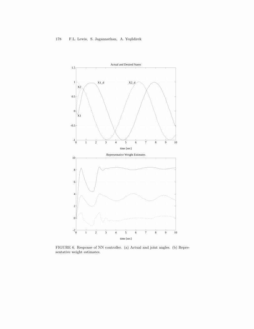
178 F.L. Lewis, S. Jagannathan, A. Yesildirek
-1
-0.5
0
0.5
1
1.5
0 1 2 3 4 5 6 7 8 9 10
time [sec]
X1
X2
X2_dX1_d
Actual and Desired States
-2
0
2
4
6
8
10
0 1 2 3 4 5 6 7 8 9 10
time [sec]
Representative Weight Estimates
FIGURE 6. Response of NN controller. (a) Actual and joint angles. (b) Repre-sentative weight estimates.

7. Neural Network Control of Robot Arms 179
-1.5
-1
-0.5
0
0.5
1
0 1 2 3 4 5 6 7 8 9 10
time [sec]
X1
X2
X2_dX1_d
FIGURE 7. Response of controller in Fig. 2 without NN. Actual and desiredjoint angles.

180 F.L. Lewis, S. Jagannathan, A. Yesildirek
rζ
Robust Term
-v(t)
’-w~ T
Tune V
Tune Wζ
σ V xT~^
2
1
^
^
.M r + ( K + V ) rmv
ω(τ) Error Dynamics
FIGURE 8. Neural net closed-loop error system

7. Neural Network Control of Robot Arms 181
L ≤ rT [−WT (σ − σ′V T x)] − κ‖r‖(‖W‖2F − ‖W‖F ‖‖W‖F )
≤ rT [−WT (σ − σ′V T x)] − κ‖r‖(‖W‖2F − WM‖W‖F ) (57)
which is in power form with the last function quadratic in WF .2. Selecting the nonnegative function
L =12tr(V T G−1V )
and evaluating L yields
L = tr(V T G−1 ˙V ) (58)
= rT (−WT σ′V T x) − κ‖r‖(‖V ‖2F− < V , V >F ) (59)
≤ rT (−WT σ′V T x) − κ‖r‖(‖V ‖2F − VM VF ) (60)
which is in power form with the last function quadratic in ‖VF ‖.Thus, the robot error system in Figure 8 is state strict passive (SSP) and
the weight error blocks are SSP; this guarantees the SSP of the closed-loopsystem (cf. [SL91]). Using the passivity theorem one may now concludethat the input/output signals of each block are bounded as long as theexternal inputs are bounded. Now, the state-strictness of the passivityguarantees that all signals internal to the blocks are bounded as well. Thismeans specifically that the tracking error r(t) and the weight estimatesW (t), V (t) are bounded (since W ,W, V , V are all bounded).
We define a NN as robust if, in the error formulation, it guarantees theSSP of the weight tuning subsystems. Then, the weights are bounded ifthe power into the system is bounded. Note that: (1) SSP of the open-loopplant error system is needed in addition for tracking stability, and (2) theNN passivity properties are dependent on the weight tuning algorithm used.It can be shown, for instance, that using only the first (backprop) terms inweight tuning as in (42), (43), the weight tuning blocks are only passive, sothat no bounds on the weights can be concluded without extra (persistenceof excitation) conditions.
5.2 Partitioned Neural Nets and Preprocessing of Inputs
A major advantage of the NN approach is that it allows one to partition thecontroller in terms of partitioned NN or neural subnets. This (1) simplifiesthe design, (2) gives added controller structure, and (3) makes for fasterweight tuning algorithms.
Partitioned Neural NetsIn [OSF+91] a NN scheme was presented for robot arms that used separateNNs for the inertia and Coriolis terms in (12). We now give a rigorousapproach to this simplified NN structure.

182 F.L. Lewis, S. Jagannathan, A. Yesildirek
The nonlinear robot function (12) is
f(x) = M(q)ζ1(t) + Vm(q, q)ζ2(t) + G(q) + F (q), (61)
where for controls purposes, ζ1(t) = qd + Λe, ζ2(t) = qd + Λe.Let q ∈ IRn. Taking the four terms in f(x) one at a time, use separate
NN to reconstruct each one so that
M(q)ζ1(t) = WTMσM (V T
MxM )
Vm(q, q)ζ2(t) = WTV σV (V T
V xV ) (62)
G(q) = WTG σG(V T
G xG)
F (q) = WTF σF (V T
F xF ). (63)(64)
Now, write f(x) as
f(x) = [WTM WT
V WTG WT
F ]
σM
σV
σG
σF
(65)
so that σ(.) is a diagonal function composed of the activation functionvectors σM , σV , σG, σF of the separate partitioned NNs. Formulation 65reveals that the theory developed herein for stability analysis applies whenindividual NNs are designed for each of the terms in f(x).
This procedure results in four neural subnets, which we term a structuredNN, as shown in Figure 9.. It is direct to show that the individual par-titioned NNs can be separately tuned, making for a faster weight updateprocedure. That is, each of the NN in (63) can be tuned individually usingthe rules in Theorem 4.6.
Preprocessing of Neural Net Inputs
The selection of a suitable x(t) for computation remains to be addressed;some preprocessing of signals, as used in Example 4.1, yields a more advan-tageous choice than (50) since it already contains some of the nonlineari-ties inherent to robot arm dynamics. Let an n-link robot have nr revolutejoints with joint variables qr, and np prismatic joints with joint variablesqp. Define n = nr + np. Since the only occurrences of the revolute jointvariables are as sines and cosines, transform q = [qT
r qTp ]T by preprocessing
to [cos(qr)T sin(qr)T qTp ]T to be used as arguments for the basis functions.
Then the vector x can be taken as
x = [ζT1 ζT
2 cos(qr)T sin(qr)T qTp qT sgn(q)T ]T ,
(where the signum function is needed in the friction terms).

7. Neural Network Control of Robot Arms 183
.
..
..
..
..
.
.
.
.
fe
e
q
q
q
q
q
q
q, q
G(q)
F(q)
M(q) ζ1
d
d
d
mV (q,q)ζ
2
..
.
..
..
^
ζ
ζ
ζ
ζ
Σ
FIGURE 9. Structured neural net.
6 Neural Networks for Control of NonlinearSystems
In this section, for a class of continuous-time systems, we will give a designprocedure for multilayer NN controller. That is, a stable NN adaptationrules and feedback structures will be derived so that systems of interestperform a desired behavior while all the generated signals remain bounded.
6.1 The Class of Nonlinear Systems
When the input/output representation of a plant is in “affine form,” theproblem of control is significantly simplified. Consequently, there has beenconsiderable interest in studying those systems. Consider a single-inputsingle-output (SISO) system having a state space representation in theBrunovsky canonical form
x1 = x2
x2 = x3
...xn = f(x) + u + dy = x1
(66)
with a state vector x = [x1, x2, . . . , xn]T , bounded unknown disturbancesd(t), which is bounded by a known constant bd, and an unknown smoothfunction f : IRn → IR.

184 F.L. Lewis, S. Jagannathan, A. Yesildirek
6.2 Tracking Problem
Control action will be used for output tracking, which can be described as,given a desired output, yd(t), find a bounded control action, u(t), so thatthe plant follows the desired trajectory with an acceptable accuracy (i.e.bounded-error tracking), while all the states remain bounded.
For this purpose we will make some mild assumptions which are widelyused. First define a vector
xd(t) =
yd
yd
...y(n−1)d
.
The desired trajectory, xd(t) is assumed to be continuous, available formeasurement and have a bounded norm,
‖xd(t)‖ ≤ Q, (67)
with Q a known bound.
6.3 Error Dynamics
Define a state error vector as
e = x − xd (68)
and a filtered error asr = ΛT e (69)
where Λ = [Λ 1]T with Λ = [λ1, λ2, · · · , λn−1] is an appropriately chosencoefficient vector so that the state error vector e(t) exponentially goes to 0as the filtered error r(t) tends to 0, i.e. sn−1 +λn−1s
n−2 + · · ·+λ2s+λ1 isHurwitz. Then, the time derivative of the filtered error can be written as
r = f(x) + u + Yd + d (70)
with
Yd = −x(n)d +
n−1∑i=1
λiei+1.
Next we will construct a NN controller to regulate the error systemdynamics (70) which guarantees that the desired tracking performance isachieved.
6.4 Neural Network Controller
If we knew the exact form of the nonlinear function f(x), then the controlaction
u = −f(x) − Kvr − Yd

7. Neural Network Control of Robot Arms 185
would bring the r(t) to zero exponentially for any Kv > 0 when there wasno disturbance d(t). Since, in general, f(x) is not exactly known to us wewill choose a control signal as
uc = −f(x) − Kvr − Yd + v (71)
where the estimate of f(x) is f(x) and the auxiliary robustifying term v(t)will be revealed later that provides robustness. Hence, the filtered errordynamics (70) becomes
r = −Kvr + f + d + v (72)
As shown in Theorem 2.1, multilayer neural networks which have linearactivation in the input and output layers and nonlinear activation functionin the hidden layer can approximate any continuous function uniformly ona compact set arbitrarily well provided that enough neurons are used. Letf(x) be a continuous function, then there exists best set of weights W andV such that the equation
f(x) = WT σ(V T x) + ε (73)
holds for any ε > 0. Therefore, f(x) may be constructed by a multilayerneural network as
f(x) = WT σ(V T x), (74)
Using the steps similar to Section 4.3, we can write the functional approx-imation error by using Taylor series expansion of σ(V T x) as
f(x) = WT (σ − σ′V T x) + WT σ′V T x + w (75)
with, (cf. (33)),
|w(t)| ≤ C0 + C1‖Z‖F + C2|r|‖Z‖F (76)
where Cis are some computable constants and the generalized weight ma-trix Z is defined in (18). In the sequel, ‖ · ‖ will indicate Frobenius norm,unless otherwise mentioned. Also recall that the Frobenius norm of a vectoris equivalent to its 2-norm, i.e. these norms are compatible.
6.5 Stable NN Control System
In order to give theoretical justification for the proposed controller struc-ture which is shown in Fig. 10, we will choose NN weight update rulesas
˙W = M(σ − σ′V T x)r − κ|r|MW˙V = NrxWT σ′ − κ|r|NV.
(77)
Now, we can reveal the stability properties of the system (66) by the fol-lowing theorem.

186 F.L. Lewis, S. Jagannathan, A. Yesildirek
rK v
T
- --
f(X)^
Plantxx
|| Z ||^
d
ΛT -
xd
(n)
e
u
Tracking-Loop
Inner-Loop
0 Λ_
FIGURE 10. Neural network controller.
Theorem 6.6 Assume that the system has a representation in the reach-ability form as in (66) and the control input is given by (71) with theauxiliary control signal
v = −Kz(‖Z‖ + Zm) (78)
with Kz ≥ C2 > 0. Let the neural net weight update law be provided by(77). Then the filtered tracking error r(t), neural net weight error Z areUUB with specific bounds giving by (82).
Proof: Since f(x) is continuous in x, then the NN approximation propertyholds in any compact subset of IRn. Given xd(t) ∈ Ud define a bound bx
so that U = x | ‖x‖ ≤ bx and Ud ⊂ U . Let |r(0)| ≤ br with br defined in(82).
Substitution of the functional approximation error as shown in (75) intothe error system dynamics for f yields
r = −Kvr + WT (σ − σ′V T x) + WT σ′V T x + d + w. (79)
Let the Lyapunov function candidate be
L =12r2 +
12tr
WT M−1W
+12tr
V T N−1V
(80)
Now substitute (79) into the time derivative of (80) and perform a simplemanipulation, (i.e. using the equality
xT y = trxT y
= tr
yxT
,

7. Neural Network Control of Robot Arms 187
one can place weight matrices inside a trace operator) to obtain
L = −Kvr2 + tr
WT (σ − σ′V T x)r + M−1 ˙W
+tr
V T (xrWT σ′ + N−1 ˙V )
+ r(d + w).
With the update rules given in (77) one has
L = −Kvr2 + r(d + w + v) + κ|r|trZT ZFrom the inequality
tr
ZT Z
=< ZT , Z > −tr
ZT Z≤ ‖Z‖(Zm − ‖Z‖),
it follows that
L ≤ − Kvr2 + r(d + w + v) + κ|r|‖Z‖(Zm − ‖Z‖).Substitute the upper bound of w according to (76), bd for disturbances andv from (78) to yield
L ≤ −Kvr2 − Kz(‖Z‖ + Zm)r2 + κ|r|‖Z‖(Zm − ‖Z‖)+[C2‖Z‖|r| + C1‖Z‖ + (bd + C0)
]|r|
Picking Kz > C2 and completing the squares yields
L ≤ −|r|
Kv|r| + κ(‖Z‖ − C3/2)2 − D1
(81)
whereD1 = bd + C0 +
κ
4C2
3 ,
andC3 = Z
m+ C1/κ.
Observe that the terms in braces in (81) defines a compact set aroundthe origin of the error space (|r|, ‖Z‖) outside of which L ≤ 0. We can,therefore, deduce from (81) that, if either |r| > br or ‖Z‖ > bf then L ≤ 0where
br =D1
Kv, bf =
C3
2+
√D1
κ. (82)
Note that br can be kept small by adjusting the design parameter Kv
which ensures that x(t) stays in the compact set U . Thus, NN approxima-tion property remains valid. According to a standard Lyapunov theoremextension, (cf. Theorem 4.6), this demonstrates the UUB of both |r| and‖Z‖. This concludes the proof.
The NN functional construction error ε, the bounded disturbances, thenorm of the desired performance and the neural network size are all con-tained in the constants Cj , and increase the bounds on error signals. Nev-ertheless, the bound on the tracking error may be kept arbitrarily small byincreasing the gain Kv. Therefore, for the class of systems, stability of theclosed-loop system is shown in the sense of Lyapunov without making anyassumptions on the initial weight values. We may simply select Z(0) = 0.

188 F.L. Lewis, S. Jagannathan, A. Yesildirek
-2
-1.5
-1
-0.5
0
0.5
1
1.5
2
2.5
-3 -2 -1 0 1 2 3
X 2
X 1
FIGURE 11. State trajectory of the van der Pol’s system.
Example 6.1
Let us illustrate the stable NN controller design on a Van der Pol’s system
x1 = x2
x2 = (1 − x21)x2 − x1 + u
(83)
which is in the Brunovsky canonical form. Note that (83) has an unstableequilibrium point at the origin x = (0, 0) and a stable limit cycle. A typicaltrajectory for this system is illustrated in Figure 11.
The neural net which is used for estimation of f(x1, x2) = (1−x21)x2−x1
consists of 10 neurons. Design parameters are set to Kv = 20, Λ = 5,Kz = 10, Zm = 1, M = N = 20, and κ = 1. Initial conditions are Z(0) = 0and x1 = x2 = 1. The desired trajectory is defined as yd(t) = sin t.Actual and desired outputs are shown in Figures 12 and 13. Recall thatthe dynamic model (83) has not been used to implement the NN-basedcontrol of Theorem 6.6. The control input is illustrated in Figure 14.
7 Neural Network Control with Discrete-TimeTuning
In Section 4 we designed a robot arm Neural Net Controller and in Section6 a NN controller for a fairly general class of nonlinear systems. We gavealgorithms for tuning the NN weights in continuous-time; the algorithmsin those sections are virtually identical. Hover, it is often more convenient

7. Neural Network Control of Robot Arms 189
-1
-0.8
-0.6
-0.4
-0.2
0
0.2
0.4
0.6
0.8
1
0 2 4 6 8 10 12 14 16 18 20
time [sec]
Actual and Desired X1
FIGURE 12. Actual and desired state x1.
-3.5
-3
-2.5
-2
-1.5
-1
-0.5
0
0.5
1
0 2 4 6 8 10 12 14 16 18 20
time [sec]
Actual and Desired X2
FIGURE 13. Actual and desired state x2
to implement control systems in discrete-time. Therefore, in this sectionwe present discrete-time NN weight tuning algorithms for digital controlpurposes. This will also provide a connection to the usual form of tuningalgorithms based on the delta rule as used by the NN community.

190 F.L. Lewis, S. Jagannathan, A. Yesildirek
-2
-1.5
-1
-0.5
0
0.5
1
1.5
2
0 2 4 6 8 10 12 14 16 18 20
time [sec]
Con
trol
FIGURE 14. Control Input.
The notation is similar to that in previous sections, but variables arenow functions of the time index k. Though the development follows thatin section 6, the derivation and proofs for the control algorithm are morecomplex, as is usual for discrete-time analysis.
The approach in this section is unusual even from the point of viewof linear adaptive control for discrete-time systems. This is because foradaptive control of discrete-time systems, it is usual to design a controllerthat requires an estimate of some unknown function. Then one makes twoassumptions: “linearity-in-the parameters” and “certainty equivalence”.According to the former, a parameter vector is extracted from the func-tional estimate which is tuned using a derived algorithm. According to thelatter, one uses the resulting estimate for the function in the control law.A third assumption of ”persistence of excitation” is needed to show theboundedness of the parameter estimation errors.
Unfortunately, a great deal of extra analysis is needed to show that boththe tracking error and the parameter estimation error are bounded (e.g.the so called “averaging methods”). In contrast, our approach selects aLyapunov function containing both the tracking error and the functionalestimation error, so that closed-loop performance is guaranteed from thestart. It is a key factor that our work requires none of the usual assump-tions of linearity-in-the-parameters, certainty equivalence, or persistence ofexcitation. As such, this NN controller may be considered as a nonlinearadaptive controller for discrete-time systems.
7.1 A Class of Discrete-Time Nonlinear Systems
Consider an mn-th order multi-input and multi-output discrete-time non-linear system, to be controlled, given in the form

7. Neural Network Control of Robot Arms 191
TABLE 2. Neural Net Controller
NN Controller:u = −WT σ(V T x) − Kvr + v (84)
Robustifying Term:
v = −Kz(‖Z‖ + Zm) (85)
NN Weight Tuning:
˙W = M(σ − σ′V T x)r − κ|r|MW˙V = NrxWT σ′ − κ|r|NV.
(86)
Signals:e(t) = x(t) − xd(t), Tracking error (87)
r(t) = ΛT e(t), Filtered tracking error (88)
x(t) = [x1, x2, · · · , xn]T , NN input signal vector (89)
Design Parameters:Gains Kv, Kz positiveΛ a coefficient vector of a Hurwitz function.Zm a bound on the unknown target weight norms.Tuning matrices M , N symmetric and positive definite.Scalar κ > 0.
x1(k + 1) = xk
...xn−1(k + 1) = xn(k)
xn(k + 1) = f(x(k)) + u(k) + d(k) (90)
with state x(k) = [x1(k) . . . xn(k)]T with xi(k) ∈ IRm; i = 1, . . . , n, controlu(k) ∈ IRm, d(k) ∈ IRm an unknown disturbance vector acting on thesystem at time instant k with a known constant upper bound, ‖d‖ ≤ dM ,and f(x(k)) an unknown smooth function.
7.2 Tracking Problem
Given a desired trajectory and its delayed values, define the tracking erroras
en(k) = xn(k) − xnd(k),
and the filtered tracking error, r(k) ∈ IRm,
r(k) = en(k) + λ1en−1(k) + . . . + λn−1e1(k) (91)

192 F.L. Lewis, S. Jagannathan, A. Yesildirek
where en−1(k), . . . , e1(k) are the delayed values of the error , and λ1 . . . λn−1
are constant matrices selected so that det(zn−1 + λzn−2 + . . . + λn−1) isstable. Equation (91) can be further expressed as
r(k + 1) = en(k + 1) + λ1en−1(k + 1) + . . . + λn−1e1(k + 1). (92)
Using (90) in (92), the dynamics of the MIMO system can be written interms of the filtered tracking error as
r(k+1) = f(x(k))−xnd(k+1)+λ1en(k)+. . .+λn−1e2(k)+u(k)+d(k). (93)
Define the control input u(k) as
u(k) = kvr(k) − f(x(k)) + xnd(k + 1) − λ1en(k) − . . . − λn−1e2(k), (94)
with the diagonal gain matrix kv > 0, and f(x(k)) an estimate of f(x(k)).Then, the closed-loop error system becomes
r(k + 1) = kvr(k) + f(x(k)) + d(k), (95)
where the functional estimation error is given by
f(x(k)) = f(x(k)) − f(x(k)).
This is an error system wherein the filtered tracking error is driven by thefunctional estimation error.
In the remainder of this paper, equation (95) is used to focus on selectingNN tuning algorithms that guarantee the stability of the filtered trackingerror r(k). Then, since (91), with the input considered as r(k) and the out-put as e(k) describes a stable system, standard techniques [SB89] guaranteethat e(k) exhibits stable behavior.
7.3 Neural Net Controller Design
Approaches such as σ-modification [PS91], or ε-modification [Nar91] areavailable for the robust adaptive control of continuous systems wherein apersistency of excitation condition is not needed. However, modification ofthe standard weight tuning mechanisms in discrete-time to avoid a PE likecondition is, to our knowledge, yet to be investigated. In this section anapproach similar to σ or e-modification is derived for discrete-time adaptivecontrol of dynamical systems. Then, it is applied to nonlinear NN tuning.
Assume that there exist some constant ideal weights W and V for a 3-layer NN (Figure 1) so that the nonlinear function in (90)can be writtenas
f(x(k)) = WT φ(V tφ(x(k)) + ε,
where the NN reconstruction error ε(k) satisfies ‖ε(k)‖ ≤ εN , with thebounding constant εN known. It is needed to know only the existence ofsuch ideal weights; their actual values are not required. For notationalconvenience define the matrix of all the ideal weights as
Z =[
W 00 V
],
The bounding assumption provided in Section 4.1 is needed on the idealweights with the bound on ‖Z‖ denoted in this section as ZM .

7. Neural Network Control of Robot Arms 193
Structure of the NN Controller and Error System Dynamics
Now suppose the estimate for f(x(k)) is provided by a NN so that the NNfunctional estimate is
f(x(k)) = WT (k)φ(vT (k)φ(x(k)),
with W and V the current values of the weights given by the tuningalgorithms. The vector of input layer activation functions is given byφ1(k) ≡ φ1(k) = φ(x(k)). Then the vector of activation functions of thehidden layer with the actual weights at the instant k is denoted by
φ2(k) ≡ φ(V T (k)φ(x(k)).
Fact 1 The usual activation functions, such as tanh, RBF, and sigmoids,are bounded by known positive values so that
‖φ1(k)‖ ≤ φ1 max and ‖φ2(k)‖ ≤ φ2 max
The error in the weights or weight estimation errors are defined by
W (k) = W − W (k), V (k) = V − V (k), Z(k) = Z(k),
where
Z(k) =[
W 00 V
](96)
and the hidden-layer output errors are defined as
φ2(k) = φ2(k) − φ2(k).
Now the control input (94) is
u(k) = xnd(k + 1 − WT (k)φ2(k) − λ1en(k) − . . . − λn−1e2(k) + kvr(k).
The closed-loop filtered error dynamics become
r(k + 1) = kvr(k) + ei(k) + WT (k)φ2(k) + ε(k) + d(k), (97)
where the identification error is defined by
ei(k) = WT (k)φ2(k).
The proposed NN controller structure is shown in Figure 15. The output ofthe plant is processed through a series of delays in order to obtain the pastvalues of the output, and fed into the NN so that the nonlinear functionin (90) can be suitably approximated. Thus, the NN controller derived ina straightforward manner using filtered error notion naturally provides adynamical NN control structure. Note that neither the input u(k) or itspast values are needed by the NN. The next step is to determine the weighttuning updates so that the tracking performance of the closed-loop filterederror dynamics is guaranteed.

194 F.L. Lewis, S. Jagannathan, A. Yesildirek
z -1
z -1z -1
z -1
z -1
z -1
z -1
z -1
z -1
+ +
+
+
+
+
+
+
++
+
--
nd
n
1
2
n-1
1
2
n-1
λ
λ
λ
λ
λ
λ
u(k)
-
DynamicalSystem
KvI
r(k)
Weight tuning
n
ndx (k)x (k+1)
x (k)
f(x(k))^
e (k)
FIGURE 15. Digital neural net control structure
7. Neural Network Control of Robot Arms 195
7.4 Weight Updates for Guaranteed Tracking Performance
A novel NN weight tuning paradigm that guarantees the stability of theclosed-loop system (97) is presented in this section. It is required to demon-strate that the tracking error r(k) is suitably small and that the NN weightsW and V remain bounded, for then the control u(k) is bounded. The up-coming theorem shows a tuning algorithm that guarantees the performancein this case of a multilayer NN.
The theorem relies on the extension to Lyapunov theory for dynami-cal systems given as Theorem 1.5-6 in [LAD93]. The nonlinearity f(x),the bounded disturbance d(k), and the NN reconstruction error ε(k) makeit impossible to show that the first difference for a Lyapunov function isnonpositive for all values of r(k) and weight values. In fact, it is onlypossible to show that the first difference is negative outside a compact setin the state space, that is if either ‖r(k)‖ or ‖Z(k)‖ are above some spe-cific bounds. Therefore, if either norm increases too much, the Lyapunovfunction decreases so that both norms decrease as well. If both normsare small, nothing may be said about the first difference of the Lyapunovfunction except that it is probably positive, so that the Lyapunov functionincreases. This has the effect of making the boundary of a compact set anattractive region for the closed-loop system. This, however allows one toconclude the boundedness of the output tracking error and the neural netweights.
Theorem 7.6 Let the reference input r(k) be bounded and the NN func-tional reconstruction error and the disturbance bounds, εN , dM , respec-tively, be known constants. Let the weight tuning for the input and hiddenlayers be provided as
V (k+1) = V (k)−α1φ1(k)[y1(k)+B1kvr(k)]T −Γ‖I−αφ1(k)φT1 (k)‖V T (k),
(98)where y1(k) = V T (k)φ1(k), and B1 is a constant design parameter matrix.Let the weight tuning for the output layer be given by
W (k + 1) = W (k)−α2φ2(k)rT (k + 1)−Γ‖I −α2φ2(k)φT2 (k)‖W (k). (99)
In both of these Γ > 0 is a design parameter. Then, the tracking error r(k)and the NN weight estimates W and V are uniformly ultimately boundedprovided the following conditions hold:
(1) α1φ21 max < 2,
α2φ22 max < 1, (100)
(2) 0 < Γ < 1, (101)
(3) kv max <1√σ
, (102)
where σ is given byσ = β1 + κ2
1β2,
where κ1 is a bound on B1 so that ‖B1‖ ≤ κ1 and
β1 = 1 + α2φ22 max +
[−α2φ22 max + Γ(1 − α2φ
22 max)]
2
1 − α2φ22 max
, (103a)

196 F.L. Lewis, S. Jagannathan, A. Yesildirek
β2 = 1 + α1φ21 max +
[α1φ21 max + Γ(1 − α1φ
21 max]
2
2 − α1φ21 max
, (103b)
Proof: Select the Lyapunov function candidate
J = rT (k)r(k) +1α1
tr[V T (k)V (k)] +1α2
tr[WT (k)W (k)] (104a)
whose first difference is given by
∆J = ∆J1 + ∆J2, (104b)
where∆J1 = rT (k + 1)r(k + 1) − rT (k)r(k), (104c)
and
∆J2 =1α2
tr[WT (k + 1)W (k + 1) − WT (k)W (k)]
+1α1
tr[V T (k + 1)V (k + 1) − V T (k)V (k)]. (104d)
Using the tracking error dynamics (97), the term ∆J1 in (104c) is ob-tained as
∆J1 =−rT (k)[I − kT
v kv] + 2(kvr(k))T (ei(k) + WT φ2(k) + ε(k) + d(k))
× eTi (k)(ei(k) + 2WT φ2(k) + 2(ε(k) + d(k)))
+ (WT φ2(k))T (WT φ2(k) + 2(ε(k) + d(k)))
× (ε(k) + d(k)T (ε(k) + d(k)). (104e)
Considering the input and hidden (98), output (99) layer weight updates,using these in (104d) and combining with (104c), one may obtain
∆J ≤−(1 − σk2
v max)‖r(k)‖2 + 2γkv max‖r(k)‖ + ρ − [2 − α1φT1 (k)φ1(k)]
×∥∥∥∥ V T (k)φ1(k)
(1 − α1φT1 (k)φ1(k)) − Γ‖I − α1φ1(k)φT
1 (k)‖2 − α1φT
1 (k)φ1(k)
× (V T φ(k) + B1kvr(k))∥∥∥∥
2
−[1 − α2φT2 (k)φ2(k)]
×∥∥∥∥ ei(k) − (1 − α2φ
T2 (k)φ2(k)) + Γ‖I − α2φ2(k)φT
2 (k)‖1 − α2φT
2 (k)φ2(k)
× (kvr(k) + WT φ2(k) + ε(k) + d(k))∥∥∥∥
2
+1α1
‖I − α1φ1(k)φ1(k)‖2 tr[Γ2V T (k)V (k) + 2ΓV T V (k)]
+1α2
‖I − α2φ2(k)φ2(k)‖2 tr[Γ2WT (k)W (k) + 2ΓWT W (k)], (105)

7. Neural Network Control of Robot Arms 197
where
γ = β1(Wmaxφ2 max + εN + dM + Γ(1 − α2φ22max)‖φ2 maxWmax +
+κ1(β2 + Γ(1 − α1φ21max)φ1 maxVmax,
and
ρ = [β1(Wmaxφ2 max + εN + dM ) + 2Γ(1 − α2φ22max)‖φ2 maxWmax]
(Wmaxφ2 max + εN + dM )[(β2 + Γ(1 − α1φ21max)φ2
1 maxV2max].
Completing the squares for ‖Z‖(k) in (105) yields ∆J ≤ 0 as long as theconditions in (100) through (102) are satisfied and the tracking error givenis larger than
‖r(k)‖ >
1(1 − σk2
v max)
(γkv max +
√γ2k2
v max + (ρ +Γ
(2 − Γ)Z2
M ) (1 − σk2v max)
).
(106)
On the other hand, completing the squares for ‖r(k)‖ in (105) results in∆J < 0 as long as the conditions (100) through (102) are satisfied and
‖Z(k)‖ >1
Γ(2 − Γ)
(Γ(1 − Γ)ZM +
√Γ2(1 − Γ)2Z2
M + Γ(2 − Γ) θ
),
(107)where
θ = Γ2Z2M +
Γ2k2v max
1 − σk2v max
+ ρ.
Therefore ∆J ≤ 0 as long as (100) through (102) are satisfied outsidea compact set (i.e. either (106) or (107) holds). In other words, if theright hand sides of (106) and (107) are denoted as two constants δ1 and δ2
respectively, then ∆J ≤ 0 whenever ‖r(k)‖ > δ1 or ‖Z(k)‖ > δ2. Let usdenote (‖r(k)‖, ‖Z(k)‖) by a new coordinate system (ϑ1, ϑ2). Define theregion
D : ϑ|ϑ1 < δ1, ϑ2 < δ2,then there exists an open set
Ω : ϑ|ϑ1 < δ1, ϑ2 < δ2,
where δi > δi implies that D ⊂ Ω. This further implies that the Lyapunovfunction J will stay in the region Ω which is an invariant set. Therefore,from (106) or (107), it can be concluded that the Lyapunov function de-creases outside a compact set, so that the tracking error r(k) and the errorin weight estimates are UUB.Remarks: For practical purposes, (106) (107) can be considered as boundsfor ‖r(k)‖ and ‖Z(k)‖.

198 F.L. Lewis, S. Jagannathan, A. Yesildirek
The complete discrete-time NN controller is given in Table 3 and shownin Figure 15. The NN reconstruction error bound εN and the bounded dis-turbances dM affect the bounds on ‖r(k)‖ and ‖Z(k)‖ in a very interestingway. Note that small tracking error bounds may be achieved by placingthe closed-loop poles inside the unit circle and near the origin through theselection of the largest eigenvalue, kv max, of kv. On the other hand, theNN weight error estimates are fundamentally bounded by ZM , the knownbound on the ideal weights Z. The parameter Γ offers a design tradeoffbetween the relative eventual magnitudes of ‖r(k)‖ and ‖Z(k)‖; a smallerΓ yields a smaller ‖r(k)‖ and a larger ‖Z(k)‖, and vice versa.
It is important to note that the problem of initializing the net weights(referred to as symmetric breaking [RC95]) occurring in other techniquesin the literature does not arise, since when W (0) and V (0) are taken aszero, the PD term (i.e. the outer loop in Figure 15) stabilizes the plant,on an interim basis, for instance in certain restricted class of nonlinearsystems. Thus, the NN controller requires no off-line learning phase. Inother words, this algorithm exhibits a learning-while-functioning-featuresinstead of learning-then-control.
The tuning algorithms (98) and (99) are similar to the delta rule, but witha “forgetting term” added. It can be shown [JL96] that if the forgettingterm is omitted, the performance of the delta rule cannot be guaranteedwithout a stringent persistency of excitation condition.
7.5 Projection Algorithm
The theorem reveals that the NN tuning mechanisms given have a majordrawback, shared by delta rule tuning algorithms in the literature. Sinceφi(k) ∈ IRNpi , with Np the number of hidden-layer neurons in the i-thlayer and the maximum value of each hidden-node output in the i-th layeris taken as unity (as for the sigmoid), then the bounds on the adaptationgain in order to assure stability of the closed-loop system are in effect givenby
0 < α1 <2
Np,
0 < α2 <1
Np.
In other words, the upper bound on the adaptation gain at each layerdecreases with an increase in the number of hidden-layer nodes in thatparticular layer, so that learning must slow down as the NN gets largerfor guaranteed performance. This behavior has been noted in the litera-ture [MSW91] using the delta rule for tuning but never to our knowledgeexplained.
This major drawback can be easily overcome by modifying the updaterule at each layer using a projection algorithm [GS84]. To wit, replace theconstant adaptation gain at each layer by
αi =ξi
ζi + ‖φ(k)‖2, i = 1, 2, (108)

7. Neural Network Control of Robot Arms 199
TABLE 3. Discrete-Time Neural Net Controller
NN Controller:
u(k) = xnd(k + 1) − WT (k)φ2(k) − λ1en(k) − . . . − λn−1e2(k) + kvr(k)
NN weight Tuning:
V (k + 1)
= V (k) − α1φ1(k)[y1(k) + B1kvr(k)]T − Γ‖I − α1φ 1(k)φT1 (k)‖V (k)
W (k + 1)
= W (k) − α2φ2(k)rT (k + 1) − Γ‖I − α2φ2(k)φT2 (k)‖W (k)
Signals:
en(k) = xn(k) − xnd(k), tracking errorr(k) = en(k) + λ1en−1(k) + λn−1e1(k), filtered tracing error
with λ1, . . . , λn−1 constant matricesselected so that det(zn−1 + λ1z
n−2 + . . . + λn−1) is stable.Design Parameters:
kv Gain matrix, positive definite.B1 a known parameter matrix.ZM a bound on the unknown target weight norms.
α1 and α2 scalar tuning rates.0 < Γ < 1 a scalar.
where ζi > 0, i = 1, 2 and 0 < ξi < 2, i = 1 are constants. Note thatξi, i = 1, 2 is now the new adaptation gain at each layer and it is alwaystrue that
ξi
ζi + ‖φi(k)‖2‖φ(k)‖2
< 2, i = 1,< 1, i = 2,
(109)
thus guaranteeing (99) for every Np at each layer.From the bounds indicated for the adaptation gains in both (100) and
(109), it is interesting to note that the upper bound on the adaptationgains for the input and hidden layers is 2 whereas for the output layer theupper bound is given by 1. It appears that the hidden layers act as patternextractors [RC95]. In other words, the hidden layers of a multilayer NNare employed for the identification of the nonlinear plant and the outputlayer is used for controlling the plant.
The weight tuning paradigm for the discrete-time NN controller is based

200 F.L. Lewis, S. Jagannathan, A. Yesildirek
on the delta rule but includes a correction term. This discrete-time NNcontroller offers guaranteed performance without a persistency of excitationcondition on internal signals. In addition, it was shown that the adaptationgains in the case of the given tuning mechanisms at each layer must decreasewith an increase in the number of hidden-layer neurons in that layer, sothat learning must slow down for large NN. The constant learning rateparameters employed in these weight tuning updates were modified using aprojection algorithm, so that the learning rate is independent of the numberof hidden-layer neurons.
Example 7.1: NN control of Discrete-Time Nonlinear System
Consider the first order multi-input multi-output discrete-time nonlinearsystem described by
[x1(k + 1)x2(k + 1)
]=
[x2(k)
1+x21(k)
x1(k)1+x2
1(k)
]+[
u1(k)u2(k)
]. (110)
The objective is to track the a periodic step input of magnitude two unitswith a period of 30 sec.
The elements in the diagonal gain matrix were chosen as
kv =[
0.1 00 0.1
]
and a sampling interval of T= 10 msec was considered. A three-layerNN was selected with 2 input, 6 hidden and 2 output nodes. Sigmoidalactivation functions were employed in all the nodes in the hidden layer.The initial conditions for the plant were chosen to be [1, − 1]T . Theweights were initialized to zero with a initial threshold value of 3.0. Nolearning is performed initially to train the network.
The response of the NN controller with weight tuning in (98) and (99)with projection algorithm (108) is illustrated in Figure 16. The design pa-rameters are selected as ξ1 = 1.0, ξ2 = 0.7 with ζ1, ζ2 chosen as 0.001. Theparameter Γ is selected as 0.01. All the elements of the design parametermatrix B1 are chosen to be 0.1. Note that with the weight tuning algo-rithms given here, the weights are guaranteed to be bounded without theneed of a PE condition.
Let us consider the case when a bounded disturbance given by
d(k) =
0.0, 0 ≤ kT < 12,0.5, kT ≥ 12.
(111)
is acting on the plant at the time instant k. Figure 17 presents the trackingresponse using the NN controller with the projection algorithm. It can beseen from the figure that the bounded disturbance induces bounded track-ing errors at the output of the plant, but the performance is satisfactory.Smaller tracking errors can be achieved by modifying kv.

7. Neural Network Control of Robot Arms 201
(a)
-5
DesiredActual
Out
put
5
4
3
2
1
0
-1
-2
-3
-4
-550 10 15 20 25 30 35 40 45 50
Time (sec)
DesiredActual
0 5 10 20 25 30 35 40 45 5015Time (sec)
5
4
3
2
1
0
Out
put
-1
-2
-3
-4
(b)
FIGURE 16. Tracking errors using discrete-time NN controller. (a) Output 1.(b) Output 2.

202 F.L. Lewis, S. Jagannathan, A. Yesildirek
DesiredActual
Time (sec)0 5 10 15 20 25 30 4035
-2.10
-1.56
-1.02
-0.48
0.06
0.60
1.14
1.68
2.22
2.76
3.30
45 50
Out
put
DesiredActual
0 5 10 15 20 25 30 4035 45 50
2.1
1.5
0.9
0.3
-0.3
-0.9
-1.5
-2.1
-3.3
-3.9
-2.7
Time (sec)
Out
put
FIGURE 17. Tracking errors with a disturbance input. (a) Output 1. (b) Output2.

7. Neural Network Control of Robot Arms 203
8 Conclusion
Continuous-time and digital Neural network (NN) controllers were designedthat give guaranteed closed-loop performance in terms of small trackingerrors and bounded controls. New NN properties such as strict passivityavoided the need for persistence of excitation. New NN controller structuresavoided the need for preliminary off-line learning, so that the NN weightsare easily initialized and the NN learns on-line in real-time. No regressionmatrix need be found, in contrast to adaptive control. No certainty equiv-alence assumption is needed, as Lyapunov proofs guarantee simultaneouslythat both tracking errors and weight estimation errors are bounded.
To guarantee performance and stability in closed-loop control applica-tions using multilayer (nonlinear) NN, it was found that the standard deltarule does not suffice, but that the NN tuning rules must be modified withextra terms.
Our primary application was NN for control of rigid robot manipulators,though a section on nonlinear system control shows how the technique canbe generalized to other classes of systems in a straightforward manner.
9 References[AS92] F. Albertini and E.D. Sontag. For neural nets, function deter-
mines form. In Proc. IEEE Conf. Decision and Control, pages26–31, December 1992.
[Bar64] R.G. Bartle. The Elements of Real Analysis. J. Wiley, NewYork, 1964.
[CK92] F.-C. Chen and H.K. Khalil. Adaptive control of nonlinearsystems using neural networks. Int. J. Control, 55(6):1299–1317, 1992.
[Cra88] J.J. Craig. Adaptive Control of Robot Manipulators. Addison-Wesley, Reading, MA, 1988.
[CS92] S.R. Chu and R. Shoureshi. Neural-based adaptive nonlinearsystem identification. In Intelligent Control Systems, ASMEWinter Annual Meeting, volume DSC-vol. 45, 1992.
[CS93] X. Cui and K.G. Shin. Direct control and coordination usingneural networks. IEEE Trans. Systems, Man, and Cybernetics,23(3), May/June 1993.
[Cyb89] G. Cybenko. Approximation by superpositions of a sig-moidal function. Mathematics of Control. Signals and Systems,2(4):303–314, 1989.
[DQLD90] D.M. Dawson, Z. Qu, F.L. Lewis, and J.F. Dorsey. Robust con-trol for the tracking of robot motion. Int. J. Control, 52(3):581–595, 1990.
[Goo91] G.C. Goodwin. Can we identify adaptive control? In Proc.European Control Conf., pages 1714–1725, July 1991.
204 F.L. Lewis, S. Jagannathan, A. Yesildirek
[GS84] G.C. Goodwin and K.S. Sin. Adaptive Filtering, Prediction,and Control. Prentice-Hall, New Jersey, 1984.
[HHA92] B. Horn, D. Hush, and C. Abdallah. The state space recurrentneural network for robot identification. In Advanced ControlIssues for Robot Manipulators, ASME Winter Annual Meeting,volume DSC-vol. 39, 1992.
[HSW89] K. Hornik, M. Stinchcombe, and H. White. Multilayer feedfor-ward networks are universal approximators. Neural Networks,2:359–366, 1989.
[IST91] Y. Iiguni, H. Sakai, , and H. Tokumaru. A nonlinear regulatordesign in the presence of system uncertainties using multilayerneural networks. IEEE Trans. Neural Networks, 2(4):410–417,July 1991.
[JL96] S. Jagannathan and F.L. Lewis. Multilayer discrete-time neu-ral net controller with guaranteed performance. IEEE Trans.Neural Networks, 7(1):107–130, Jan. 1996.
[KC91] L.G. Kraft and D.P. Campagna. A summary comparison ofcmac neural network and traditional adaptive control systems.In W.T. Miller, R.S. Sutton, and P.J. Werbos, editors, NeuralNetworks for Control, pages 143–169. MIT Press, Cambridge,MA, 1991.
[LAD93] F.L. Lewis, C.T. Abdallah, and D.M. Dawson. Control of RobotManipulators. Macmillan, New York, 1993.
[Lan79] Y.D. Landau. Adaptive Control: The Model Reference Ap-proach. Marcel Dekker, Inc., 1979.
[LC93] C.-C. Liu and F.-C. Chen. Adaptive control of nonlinearcontinuous-time systems using neural networks— general rel-ative degree and mimo cases. Int. J. Control, 58(2):317–335,1993.
[LL92] K. Liu and F.L. Lewis. Robust control techniques for generaldynamic systems. J. Intel. and Robotic Sys., 6:33–49, 1992.
[LLY95] F.L. Lewis, K. Liu, , and A. Yesildirek. Neural net robot con-troller with guaranteed tracking performance. IEEE Trans.Neural Networks, 6(3):703–715, 1995.
[LYL96] F.L. Lewis, A. Yesildirek, and K. Liu. Multilayer neural netrobot controller: structure and stability proofs. IEEE Trans.Neural Networks, 7(2):1–12, March 1996.
[MB92] G.J. Mpitsos and R.M. Burton, Jr. Convergence and divergencein neural networks: processing of chaos and biological analogy.Neural Networks, 5:605–625, 1992.
[MSW91] W.T. Miller, R.S. Sutton, and P.J. Werbos, editors. NeuralNetworks for Control. MIT Press, Cambridge, MA, 1991.

7. Neural Network Control of Robot Arms 205
[NA87] K.S. Narendra and A.M. Annaswamy. A new adaptive law forrobust adaptation without persistent excitation. IEEE Trans.Automat. Control, AC-32(2):134–145, Feb. 1987.
[Nar91] K.S. Narendra. Adaptive control using neural networks. InW.T. Miller, R.S. Sutton, and P.J. Werbos, editors, Neural Net-works for Control, pages 115–142. MIT Press, Cambridge, MA,1991.
[NP90] K.S. Narendra and K. Parthasarathy. Identification and con-trol of dynamical systems using neural networks. IEEE Trans.Neural Networks, 1:4–27, March 1990.
[OSF+91] T. Ozaki, T. Suzuki, T. Furuhashi, S. Okuma, and Y. Uchikawa.Trajectory control of robotic manipulators. IEEE Trans. Ind.Elec., 38:195–202, June 1991.
[Pao89] Y.H. Pao. Adaptive Pattern Recognition and Neural Networks.Addison-Wesley, Reading, MA, 1989.
[PG89] T. Poggio and F. Girosi. A theory of networks for approxima-tion and learning. Technical Report 1140, Artificial IntelligenceLab, MIT, 1989.
[PI91] M.M. Polycarpou and P.A. Ioannu. Identification and con-trol using neural network models: design and stability anal-ysis. Technical Report 91-09-01, Dept. of Elec. Engin. Systems,Univ. Southern Calif., September 1991.
[PI92] M.M. Polycarpou and P.A. Ioannu. Neural networks as on-line approximators of nonlinear systems. In Proc. IEEE Conf.Decision and Control, pages 7–12, Tucson, AZ, Dec. 1992.
[PS91] J. Park and I.W. Sandberg. Universal approximation usingradial-basis-function networks. Neural Comp., 3:246–257, 1991.
[RC95] G.A. Rovithakis and M.A. Christodoulou. Adaptive control ofunknown plants using dynamical neural networks. IEEE Trans.Systems, Man and Cybernetics, 1995.
[RHW86] D.E. Rumelhart, G.E. Hinton, and R.J. Williams. Learning in-ternal representations by error propagation. In D.E. Rumelhartand J.L. McClelland, editors, Parallel Distributed Processing.MIT Press, Cambridge, MA, 1986.
[Sad91] N. Sadegh. Nonlinear identification and control via neural net-works. In Control Systems with Inexact Dynamics Models, vol-ume DSC-33, ASME Winter Annual Meeting, 1991.
[SB89] S.S. Sastry and M. Bodson. Adaptive Control. Prentice-Hall,New Jersey, 1989.
[SL88] J.-J.E. Slotine and W. Li. Adaptive manipulator control: a casestudy. IEEE Trans. Automat. Control, 33(11):995–1003, Nov.1988.

206 F.L. Lewis, S. Jagannathan, A. Yesildirek
[SL91] J.-J.E. Slotine and W. Li. Applied Nonlinear Control. Prentice-Hall, New Jersey, 1991.
[SS91] R.M. Sanner and J.-J.E. Slotine. Stable adaptive control andrecursive identification using radial gaussian networks. In Proc.IEEE Conf. Decision and Control, Brighton, England, 1991.
[Sus92] H.J. Sussmann. Uniqueness of the weights for minimal feed-forward nets with a given input-output map. Neural Networks,5:589–593, 1992.
[Wer74] P.J. Werbos. Beyond Regression: New Tools for Prediction andAnalysis in the Behavioral Sciences. PhD thesis, Committee onApplied Math., Harvard Univ., 1974.
[Wer89] P.J. Werbos. Back propagation: past and future. In Proc. 1988Int. Conf. Neural Nets, volume 1, pages 343–I353, 1989.
[YL95] A. Yesildirek and F.L. Lewis. Feedback linearization using neu-ral networks. Automatica, 31(11):1659–1664, Nov. 1995.
[YY92] T. Yabuta and T. Yamada. Neural network controller charac-teristics with regard to adaptive control. IEEE Trans. Systems,Man and Cybernetics, 22(1):170–176, Jan. 1992.

8
Neural Networks for IntelligentSensors and Control —Practical Issues and SomeSolutions
S. Joe Qin
ABSTRACT Multilayer neural networks have been successfully applied asintelligent sensors for process modeling and control. In this paper, a fewpractical issues are discussed and some solutions are presented. Severalbiased regression approaches, including ridge regression, PCA, and PLS,are integrated with neural net training to reduce the prediction variance.
1 Introduction
The availability of process control computers and associated data histo-rians make it easy to generate neural network solutions for process mod-eling and control. Numerous applications of neural networks in the fieldof process engineering have been reported in recent annual meetings andtechnical journals. Neural network solutions are well accepted in processindustries since they are cost-effective, easy-to-understand, nonlinear, anddata-driven.
This chapter addresses several practical issues and some solutions re-garding to use of neural networks for intelligent sensors and control. Thechapter begins with an introduction to neural network applications as in-telligent soft sensors to predict process variables that are not measurableon-line. Then several practical issues in the intelligent sensor applicationsare presented: (i) outlier detection and missing value treatment; (ii) vari-able selection; (iii) correlated input data versus network training, predictionand control; and (iv) neural network training and validation. Approachesto integrating biased statistical methods with neural network training arediscussed to handle correlated input data. The integration of neural net-works with partial least squares is discussed and illustrated with a realprocess application. Last, conclusions are given and further issues are rec-ommended for future investigation.
Artificial neural networks have found many applications in process mod-eling and control. These applications include: (i) building intelligent softsensors to estimate variables which usually need to be measured through labtests (McAvoy, et al. [M+89]; Willis, et al [WDM+91]); (ii) dynamic systemidentification (Bhat, et al. [BMMW90]; Narendra, et al [NP90]); (iii) faultdetection and diagnosis (Venkatasubramanian, et al. [VVY90]; Ungar, et

208 S. Joe Qin
al. [UPK90]); (iv) process data screening and analysis (Kramer [Kra92]);and (v) use of neural nets for control (Hernandez and Arkun [HA90];Hoskins and Himmelblau, et al. [HH92]).
Among all types of neural networks, multilayer feedforward networks(MFN, Rumelhart, et al. [RHW86]) have primarily been applied in processmodeling and control. There are a number of reasons that can explain whyMFN’s are widely applied to process industries. First of all, multilayer feed-forward networks are good nonlinear function approximators. A number ofresearchers (Hornik, Stinchcombe and White [HSW89]; Cybenko [Cyb89])have proven that an MFN can approximate any continuous function suffi-ciently well. Since many chemical processes are highly nonlinear, the non-linear capability of neural nets is promising to process engineers. Second, aneural network can be trained to learn a chemical process by using histor-ical process data. With plenty of process data available from distributedcontrol systems in industrial processes, building a neural network based onprocess data is cost-effective. The third reason is the ease of use for processengineers. Building a neural network model does not necessarily require asmuch knowledge as the first principles approach or statistical approaches,although fundamental understanding of the process is required.
Owing to the availability of distributed control systems (DCS) and asso-ciated database historians in process industries, huge amounts of historicaldata exist that can be used for neural network applications without addi-tional investment. Typically, the historical data have been poorly utilizedin the past, although much useful information could be extracted from thedata. This is one of the areas in process industries where neural networkscan be applied without further investment in data acquisition. One suchapplications is to predict key process variables that cannot be measuredon-line. This type of applications is known as soft sensor or intelligent sen-sor. The hard-to-measure variables are usually quality variables or directlyrelated to the economic interest of the production. These quality variablesare often observed from analyzing product samples off-line in a laboratory.An obvious time-delay is incurred in analyzing the test samples, which canbe in the range of one to ten hours. Although one could know the productquality after this delay, it might be too late to make timely control adjust-ment if required. Figure 1 illustrates the intelligent sensor application usingneural networks. A neural network is trained on historical data to predictprocess quality variables so that it can replace the lab-test procedure. Animmediate benefit of building intelligent sensors is that the neural networkcan predict product quality in a timely manner. If the product quality doesnot meet the requirement and hence a correction is needed, the intelligentsensors allow early control actions to be made, which can avoid continuingmanufacturing of poor quality product.
This chapter presents a few practical issues that are often encounteredin using neural networks for intelligent soft sensors and control. Theseissues are: (i) data preprocessing, including missing values and outlier de-tection; (ii) variable selection; (iii) network training and control issues withcorrelated variables; and (iv) integrating statistical approaches and neuralnetwork for intelligent sensors.
The organization of the chapter is as follows. Section 2 discusses thetypical characteristics of historical process data. Section 3 addresses theissues in data pre-processing, including outlier detection and missing valuereplacement. Section 4 presents the issue of variable selection in deal-ing with real applications. Sections 5 analyzes the effect of collinearity

8. Intelligent Sensors and Control 209
Process input
Process
Process Quality
Quality Prediction
Lab-test
FIGURE 1. Use of neural networks as intelligent sensors to predict processquality variables that can only be measured through lab test.
on neural network training, generalization, and control. Section 6 presentsapproaches to integrating neural networks with statistical methods are pre-sented, including partial least squares (PLS), principal component analysis(PCA), and ridge regression. Section 7 uses a real application exampleto illustrate how the integrated approach may outperform a direct neuralnetwork approach. The final section gives concluding remarks.
2 Characteristics of Process Data
Most industrial processes are well equipped with on-line process sensors,such as temperature, flowrate, and pressure sensors, and in some cases ana-lytical sensors. These sensors allow the process computer to acquire on-lineprocess information and make appropriate control to maintain consistentproduct quality. Most of the control strategies are feedback control, wherePID control and model-based control are dominant. A data historian thatcollects and stores historical data is usually linked to the process computer.Some variables, especially the quality variables, do not have on-line sensors,or the available sensors are not cost-effective or reliable. However, sincethese variables are of crucial importance, lab tests of the product samplesare usually conducted to measure the product quality off-line on a specifiedinterval base.
In the situation where lab tests are conducted, a time-delay of one toten hours is often incurred. In order to detect the quality variables in atimely manner, one can build intelligent sensors to infer the quality vari-ables from other on-line measured process variables. The foundation ofbuilding intelligent sensors is that the product quality variables have afunctional relationship with other process variables that can be measuredon-line, such as compositions of raw materials, temperature, pressure, andresidence time during which the product is made. Since the functionalrelationship between the quality variables and other variables are usuallynonlinear, the neural network approach is a convenient choice for modelingthe relationship.
The neural network approach to building intelligent sensors is funda-mentally an empirical approach based on process data. This approach is

210 S. Joe Qin
efficient when alternative approaches such as the first principles approachare difficult or too expensive to obtain. However, one of the difficultiesinvolved in the neural network approach is that many issues are not welldefined and have to be determined based on data analysis. These issuesinclude data acquisition, outliers and missing values, input variable selec-tion, and variable collinearity. Practical experience shows that resolvingthese issues takes much more time than training a neural network.
There are three categories of data that could be used to build intelligentsensors. The first category is historical data that are collected from on-linesensors during the process operation. Most of the available data are inthis category. The nature of the historical data is known as data-rich andinformation-poor (Piovoso [PO91]). Usually, a large portion of the datais collected under a particular operating condition. Relatively little infor-mation is available under other operating conditions. In order to collectdata that cover various types of operating conditions, one needs to use datathat cover a long period of history. In the case where the process is slowlyvarying over time or where significant change was made in the process, olddata may be obsolete and useless for building intelligent sensors for thecurrent process. Therefore, a trade-off is needed in data acquisition to getthe greatest amount of truly representative data.
The second category of data is lab-test data that are collected for hard-tomeasure quality variables. These data are often available with much largertime intervals than the historical data. Typically the lab-test data are notcollected at a regular rate. This is due to the fact that the lab-test is doneby a human being instead of a digital computer. Further, the lab-test dataoften have missing data points. The sampling rate must be regularizedwith interpolation or other techniques. When there are missing values inthe lab-test data, they should be either replaced or not used for training aneural network. Dayal, et al. [DMT+92] discussed a practical treatment ofmissing values in this regard.
The third category of data are experimental data that can be collectedby conducting an experimental design. This category of data is most de-sirable in terms of the data quality, but it is often not available due to thehigh cost of obtaining it or because of safety considerations. Sometimes anexperimental design may be allowed to collect a few samples as a comple-mentary approach to the historical data. In this chapter, we focus on thecase where the experimental data are generally not available for intelligentsensor modeling.
Building intelligent sensors based on historical and lab-test data is a pas-sive approach, since no experimental designs are conducted. This approachhas the least intervention to process operation. Therefore, it is generallyapplicable to all kinds of processes. However, due to the limited informa-tion content in the historical data, the resulting intelligent sensors are validonly on the particular region in which the data are collected. Therefore, itis important to identify the valid region associated with the intelligent sen-sor. It is necessary, though not sufficient, to check the lower-upper boundsfor new data when a trained neural network is implemented on-line. Whenthe process operation changes significantly, the intelligent sensor has to bere-calibrated on new data in order to give a valid prediction.

8. Intelligent Sensors and Control 211
3 Data Pre-processing
Before training a neural network, data preprocessing is normally requiredsince most of the historical data and lab-test data are not ready to use fortraining. The first step in pre-processing is to identify and remove outliers,since industrial data bases typically have outliers. Outliers are treated instatistics as samples that carries high leverage (Martens, et al. [MN89]), yetare so few to be statistically meaningful. Outliers can result from sensorfailure, misreading from lab tests, and other unknown upsets to the process.Some outliers can be normal data and represent important information, butadditional knowledge is needed to discriminate them against bad outliers.A distinctive feature of outliers is that they normally have extremely largeinfluence on the model. Since neural network training employs a leastsquares type of objective function with individual training error,
Ei =p∑
j=1
(yij − yij)2 (1)
or cumulative training error,
E =1N
N∑i=1
Ei (2)
which is generally sensitive to outliers with large model errors (Kosko[Kos92]). Although it is felt that a neural network training scheme whichincludes both training and testing might stop training before overfittingthe outliers, there is no guarantee that network training will ignore outliersand fit well on good samples. This scheme is even less reliable when thereare outliers in the test set. Further, since neural networks can be extremelynonlinear, it is experienced that neural networks are more sensitive to out-liers than linear regression methods because they can bend to reach theoutliers. As a consequence, it is necessary to perform outlier detection andpre-treatment before training the network .
3.1 Obvious OutliersSome outliers are so obvious that they can be identified by using priorknowledge and physical laws. For example, a temperature variable cannotreach below absolute zero degree, and a flowrate variable cannot be neg-ative. Generally, one can determine the possible maximum and minimumvalues of a process variable based on experience. Therefore, some outlierscan be identified simply by checking them against the minimum and max-imum. If a sample is below the minimum or above the maximum, it isconsidered as an outlier. Although this method is very simple, it is usefulfor preliminary detection of outliers. Another reason to establish maximumand minimum values is to define the operating region of interest. If the dataare outside the region of interest, they should be considered outliers.
After identifying the outliers, a number of approaches can be taken totreat outliers. First, an outlier can be replaced by the maximum or mini-mum value. Since we do not know the real value of the outlier, this approachis often not reliable. A conservative approach is to replace the outlier with

212 S. Joe Qin
the mean of the process variable. The third approach is to treat them asmissing data, which will be discussed later.
3.2 Non-obvious OutliersIn contrast to the obvious outliers, many outliers lie within the boundariesand are hard to identify. They do not violate the minimum and maximum,but they can cause large model errors because they violate other physicalconstraints. For example, the pressure and flowrate is supposed to havequadratic relationship by physical principles, but an outlier may violatethis relation. In many cases, the process data are highly correlated. Ifsome samples appear to be not correlated, they are considered outliers be-cause they violate the correlation structure. These outliers can be detectedusing statistical methods such as principal component analysis (Wold, etal. [WEG87]) and partial least squares (Martens, et al. [MN89]).
Outliers can also be detected by examining the signals in the frequencydomain. For example, a temperature variable has a certain frequency limit.It cannot change too frequently because temperature is a slow process. Ifthe variable is identified as having impossibly high frequency components,it is considered as having outliers. A properly designed filter can be used tofilter out the effect of outliers. In order to overcome phase lags introducedby using low-pass filters, Piovoso, et al. [PO91] used the FIR median hybridfilters to extract steady state information. The filtering approach is mosteffective when an entire variable is heavily corrupted with noise.
3.3 Robust Backpropagation
Despite the various outlier detection techniques applied to the data, thereare usually some outliers left in the data set. Therefore, it is importantto use some training methods that are insensitive to outliers. As indicatedearlier, a distinct feature of outliers is that they carry large individual train-ing errors. Since the regular backpropagation algorithm uses least squarestraining error, it is sensitive to large training errors and thus sensitive tooutliers (Kosko [Kos92]). Robust backpropagation that is insensitive tooutliers can be developed by borrowing the techniques from robust regres-sion methods. Instead of having a least squares training error that amplifieslarge training errors, one can use the following training error that treatsthe large errors and small errors linearly:
Ei =p∑
j=1
|yij − yij | (3)
This error function can reduce the influence of outliers that carry largeindividual errors. Another approach that uses suppressing functions isgiven in Kosko [Kos92].
3.4 Missing Values
Missing values are very common in historical data bases from distributedcontrol systems and lab test data. In general, it is difficult for multilayer

8. Intelligent Sensors and Control 213
neural networks to handle missing values during training. Therefore, it isnecessary to pre-process missing values before training. There are a numberof ways to handle missing values. A simple way to deal with missing valuesis to delete samples that have missing values. However, if the availabledata are limited, and the missing values are not clustered together, onecan apply the techniques of missing data replacement to keep as manysamples as possible.
When the missing values are not clustered together, it is reasonable toapply interpolation to replace the missing values. Dayal, et al. [DMT+92]apply linear interpolation when there are less than three consecutive miss-ing points. Of course, it is possible to apply other interpolation techniquessuch as cubic splines. However, when there are more consecutive missingvalues, it is not reliable to apply interpolation. More advanced techniqueshave to be applied.
As long as the missing values are evenly distributed over the data set,there are statistical methods such as principal component regression (PCR)and partial least squares (PLS) which can work with data sets that havemissing values (Geladi & Kowalski [GK86]; Wold, et al. [WEG87]). Thesemethods perform principal component or principal factor calculations andthen build regression models based on them. They allow some “holes“ inthe data set. Therefore, one can apply principal component analysis on thetraining data with some missing values, then build a neural network modelbased on the principal components. One can handle the missing values inthe calculation of principal components. One can also integrate the partialleast squares with neural networks to handle the missing value problem.Another benefit of integrating these statistical methods with neural net-work training is to handle the correlated variables that can cause largevariance on the prediction. Details of the integration of neural networksand partial least squares can be found in Qin and McAvoy [QM92b].
If the process variables are highly correlated in a nonlinear manner,auto-associative neural networks can be used to recover the missing val-ues (Kramer [Kra92]). The auto-associative neural networks are specialtypes of feedforward networks which have identical input and output vari-ables. The auto-associative networks re-construct the variables from othervariables that are cross-correlated in a linear or nonlinear manner. Thiscorrelation offers fundamental redundancy for recovering missing values. Itshould be noted that, to recover a variable that has a missing value, it mustbe highly correlated to other variables that do not have missing values. Itis not possible to recover a missing value of a variable that has no correla-tion with other variables. An alternative approach to the auto-associativenetworks is the principal curve approach integrated with neural networks(Dong and McAvoy [DM94]). This approach provides a natural nonlinearextension to principal component analysis.
4 Variable Selection
! An industrial data base usually provides all the variables that can berecorded. However, it is not necessarily true that all recorded variables arerelevant to the process variables to be predicted. Instead, it is often the casethat when some of the irrelevant variables are deleted from the data base,the modeling results can be improved; if the irrelevant variables are kept inthe model, they play a role of noise which can potentially deteriorate the

214 S. Joe Qin
modeling results. Therefore, it is imperative to select a subset of processvariables that are truly relevant to the predicted variables. Prior knowledgecan be used to screen out totally irrelevant variable, but further approachesare needed finally select relevant variables.
The issue of variable selection has been studied in regression analysis(Hocking [Hoc76]). The more the variables are used in a model, the worsethe prediction variance is, and the better the prediction bias. Basically,each process variable to be used in a model contributes a value to the pre-diction with associated variance. When a variable’s contribution is largerthan its related variance, it is useful to the model. However, when a vari-able’s contribution is smaller that its related variance, it could be harmfulto the model.
Variable selection can be performed by judging a variable’s contributionor relevance to the predicted variables. Two typical schemes used for vari-able selection are forward selection and backward elimination among allvariables. Both the forward selection and backward elimination schemescan be used in neural network training. In a forward selection scheme,one starts the neural network with a small set of variables and adds morevariables if they contribute to the prediction. In the backward elimination,the neural network starts with all available variables and then eliminatesvariables that are not relevant to the prediction. However, since neuralnetwork training is involved in each selection step, these variable selectionschemes are quite laborious.
A sensitivity analysis approach is proposed in Qin and McAvoy [QM92a]to select variables in a neural net PLS scheme. In this method, sensitiv-ity analysis of model outputs with respect to model inputs is conductedover the operation region where data are collected. If the sensitivity of anoutput variable with respect to an input variable is very small, the inputvariable is deleted from the model because it has little contribution to theprediction. The sensitivity analysis provides an approach to identifying lesssensitive variables. The sensitivity is a measure of a variable’s significancein explaining the output variable. To determine if a variable is truly con-tributing to the output variable, the cross-validation method is conductedand the prediction error on the test set is calculated before and after delet-ing the variable. If the prediction error is not increased after deleting thevariable, it will be deleted from the network input; otherwise, it will be re-tained in the network input. With this method, one can achieve improvedaccuracy by deleting irrelevant variables and keeping relevant variables inthe neural network model.
A related issue is to determine the process dynamics and time delays asso-ciated with the predicted outputs. Since the process data are collected overa history of normal operation, it always contains dynamic information andtime delays. The dynamics and time delays can be included in the modelby using a time window (Qin and McAvoy [QM92a]). The time windowcontains time delayed values of input variables and output variables. Bytreating these delayed variables as individual variables, the variable selec-tion techniques can be used to determine the process dynamics and timedelays.
There is usually high correlation or redundancy among the measured pro-cess variables. Some correlation is due to the fact that a group of variablesaffect each other. Correlation can also be due to insufficient variabilityduring the normal process operation. In many situations, however, it isnot desirable to delete variables that are correlated, since the correlationoffers necessary redundancy for replacing missing values and for reducinggross errors (Kramer [Kra92]). One example is that one physical process

8. Intelligent Sensors and Control 215
variable is measured by two sensors. These two sensor measurements arecertainly correlated and using both measurements can reduce the measure-ment noise. Therefore, it is desirable to include correlated variables as longas they are relevant to the predicted variables.
However, correlated variables brings up the problem of collinearity. Inlinear statistical regression, such as the ordinary least squares approach,collinearity can cause the solution to be ill-conditioned and the resultedmodel to have large prediction variance. In this case, biased regressionapproaches such as principal component regression and partial least squaresare often used. The next section discusses the effect of collinearity on neuralnetwork modeling.
5 Effect of Collinearity on Neural NetworkTraining
5.1 Collinearity and Network Training
It is well known that collinearity presents an ill-conditioned problem toordinary least squares in linear regression. Here the effect of collinearityon neural network training is demonstrated. Given an input vector and anoutput variable y, a multi-layer neural network with one hidden layer canbe represented as follows,
y =n∑
i=0
νis(φi) (4)
φi =m∑
j=0
wijxj ; i = 1, 2, . . . , n (5)
where φi (i = 1, 2, . . . , n) is input to the i-th hidden unit. The wij andνi are weights for the input layer and output layer, respectively. s(·) isa nonlinear function of a hidden unit which can be sigmoidal. x0 ≡ 1and s(φ0) ≡ 1 stand for the bias units for the input and hidden layers,respectively. Given a sequence of samples, (x1, y1), (x2, y2), . . . , (xN , yN ),the neural network can be trained by minimizing the following error
E =1N
N∑p=1
[yp − f(xp;v,W]2 (6)
where
W ≡ [wij ] ∈ IRn×(m+1) (7)
v ≡ [ν0, ν1, . . . , νn]T ∈ IRn+1 (8)
is a global function represented by Eqs. 4 and 5.If the input variables are collinear, there are many sets of weights which
can minimize the error function in Eq. 6. For example, assuming that theinput collinearity can be described by the equation
Ax = 0 (9)

216 S. Joe Qin
where A ∈ IRr×(m+1), one has the following relation for any B ∈ IRn×r,f(x;v,W) = f(x;v,W + BA) (10)
In other words, if a set of weights (v,W) minimizes the error function inEq 6, (v,W + BA) is also a solution to Eq. 6 for any B. In practice,although the variables may not be exactly collinear as in Eq. 9, they areoften highly correlated. If a backpropagation algorithm is used for training,significantly different weight distributions could result in little change inthe training error. This phenomenon is an indication of collinearity.
It is known that neural network training does not have the ill-conditionedproblem as does least squares, thus, one may think that collinearity is nota problem in neural network training. However, this is not true when pre-diction is made on new data. Since new data always include measurementnoise, the model derived from backpropagation training often results inlarge prediction variance. In other words, neural networks trained by reg-ular backpropagation tend to enlarge the noise variance in the presence ofcollinearity. This point is illustrated by analyzing the variance of predictionerror in the following subsection.
5.2 Collinearity and Prediction Variance
To illustrate how collinearity effects prediction variance, the example inMacGregor et al. [MMK+91] is used here. This example considers an ide-alized process with one output variable and five input variables that areexactly collinear. The real process relation is assumed to be
y = 1.0x2 + e (11)
The objective is to build a linear model of the five input variables andthe output variable. Since the input variables are exactly collinear, it isobvious that an ordinary least squares approach yields an ill-conditionedproblem. When the PLS method is used, the following model results,
(PLS) : y = 0.2x1 + 0.2x2 + 0.2x3 + 0.2x4 + 0.2x5 (12)
When a linear network model without hidden layers is built, three differentmodels result from different initial conditions,
(NN1) : y = 0.63x1 + 0.36x2 + 0.09x3 + 0.22x4 − 0.30x5
(NN2) : y = −0.43x1 − 0.05x2 + 0.92x3 − 0.02x4 + 0.58x5 (13)(NN3) : y = 0.23x1 + 0.35x2 − 0.26x3 − 0.22x4 + 0.91x5
These three models are adequate as long as their coefficients sum up as 1.0.Consider that new data for the five inputs have independent, identically
distributed measurement noise with zero mean and variance , the predictionvariance of the three neural network models and the PLS model can becalculated as follows,
Var(yNN1) = 0.67σ2
Var(yNN2) = 1.37σ2 (14)Var(yNN3) = 1.12σ2
Var(yNN4) = 0.200σ2

8. Intelligent Sensors and Control 217
xx
xx
xx
x
x
x
x
xx
x
x x
xx
x
x
xxx
x
x
ooo
o
o
ooo
X
X
y
valid region
2
1
FIGURE 2. A model derived from collinear data is not valid when the collinearitychanges. “x“ – collinear data for modeling; “o“ – new data when collinearitychanges.
One can see that all the neural network models result in much larger pre-diction variances than the PLS model. Although the first neural net modelreduces the variance, the other two models actually enlarge the variance.This demonstrates that backpropagation is sensitive to collinearity and re-sults in a large prediction variance.
5.3 Control of Collinear Processes
Having collinearity in a process is an indication that the number of mea-surements are greater than the degrees of freedom or variability. Somecollinear relations are inherent to the process, which do not change undernormal conditions. For example, a pump outlet pressure and flowrate arehighly correlated. Changes in these collinear relations indicates that ab-normal events occur in the process, which is useful for process monitoringand diagnosis (Wise 1991 [Wis91]). Other collinear relations are due tolack of variability in the data. This type of correlation can change whennew variability occurs in the data.
A neural net model derived from collinear data is valid only when thecorrelation holds. Figure 2 depicts an example of two collinear inputs andone output. The correlated data cluster occurs approximately on a line inthe (x1, x2) plane. When a neural net model is derived from these data,it only captures the functional relation in a subspace where x1 and x2 arecorrelated, since there are no data elsewhere for training. Therefore, thederived model is valid when the collinearity conforms. However, when newdata do not follow the correlation, the model is no longer valid and needsto be updated.
When a model from collinear data is used for control purposes, one hasto comply with the validity of the model, that is, the variables have to bemanipulated in such a way that the collinearity conforms. One cannot,for example, manipulate one variable freely and keep other variables un-changed. Another reason to change the collinearity is if a feedback loopis introduced. See MacGregor, et al. [MMK+91] for further discussion. Ifsuch a model is used for inverse control, which calculate what the inputvalues should be to achieve given output values, the inverted inputs haveto follow the correlation structure to keep the model valid.

218 S. Joe Qin
6 Integrating Neural Nets with StatisticalApproaches
6.1 Modifying Back-propagation to Minimize Variance
Since there are many solutions that satisfy the training problem in the caseof collinear data, we can use these extra degrees of freedom to minimizethe variance. In order to minimize the output variance of the neural net-work given in Eqs. 4,5, the variance of input to the hidden layer should beminimized first. Consider that each input is composed of a deterministicsignal and a random noise, i.e.,
xj = xj + εj (15)
where the measurement noise εj for each input variable is independent withzero mean and variance σ2, the variance of the hidden layer inputs can bewritten as
Var(φi) =n∑
j=1
w2ijσ
2; i = 1, 2, . . . , n (16)
To minimize the above variance while minimizing the network training errorin Eq. 6, we can minimize the following error,
Eλ = E + λ
n∑i=1
m∑j=1
w2ij = E + λ‖W‖2
2 (17)
where λ is an adjustable weighting parameter. Similarly, the output vari-ance with respect to the output layer weights should also be minimized.Therefore, we have the following error function to minimize,
Eλµ = E +12µ‖v‖2
2 = E +12(µ‖v‖2
2 + λ‖W‖22) (18)
where λ and µ are penalty factors for the magnitude of the network weights.Given many solutions that result in the same training error from Eq. 6, theabove training error chooses the one with minimum norm of weights. Theerror in Eq. 18 can be minimized by gradient descent or conjugate gradientmethods. Note that Eq. 18 is actually one application of the statisticaltechnique known as ridge regression (Hoerl, et al. [Hoe70]).
6.2 Example
To illustrate the effectiveness of variance reduction, the example given inthe preceding section is reused here. Given that the five inputs are exactlycollinear and with the constraint that the magnitude of the weights isminimized, It is easy to see that backpropagation with ridge regressionresults in the following relation,
y = 0.2x1 + 0.2x2 + 0.2x3 + 0.2x4 + 0.2x5 (19)
which gives a prediction variance of 0.2σ2.

8. Intelligent Sensors and Control 219
Although ridge regression helps backpropagation reduce the predictionvariance, it is difficult to determine the penalty factors. Practical processdata may not be exactly collinear but rather highly correlated. In this case,the penalty factors induce bias in prediction while reducing the variance.The larger the penalty factors, the smaller the variance is but the largerthe bias is. Therefore, it is important to choose the penalty factors so asto give the best model in a mean-square-error sense. Cross-validation maybe used to determine the penalty factors.
6.3 Principal Components for Neural Network Modeling
Principal component analysis (PCA) has been used to remove collinearity inlinear regression as principal component regression (PCR) (Jolliffe [Jol86]).Here, the PCA is applied to remove collinearity for neural network training.To follow the notation of PCA and PLS, the input and output data arearranged into two data matrices, X and Y, respectively. The basic idea ofPCA is to transform the data matrix X into a matrix with fewer orthogonaldimensions, while keeping most of the variance in the data matrix Xl, thatis,
T = XP (20)
where the columns of T ∈ IRm×p, known as principal components, areorthogonal. Columns of P, known as loading vectors, are orthonormal.The calculation of T and P is done by decomposing X into the followingbilinear relation,
X = TPT + R (21)where the residual R is minimized during calculation.
When the residual R can be negligible, matrix Tis completely represen-tative of matrix X. Therefore, a nonlinear relation between X and Y canbe modeled in two steps: first calculating T and then building a neural net-work between T and Y. The model structure can be depicted in Figure 3.The neural network training between the output variable and the principalcomponents can be treated as a regular network training problem. Whenthe trained model is used for prediction, it goes through a PCA calcula-tion and a neural network calculation. The combined neural network andPCA scheme offers a viable approach to overcoming collinearity in neuralnetwork training. Since the principal components are orthogonal, they canbe used for analyzing the features of the data and for monitoring processchanges. A limitation of the neural net PCA approach is that PCA focusesonly on the variance of inputs which may ignore the inputs’ correlation tothe output. A component that is non-principal in PCA analysis can besignificant in explaining the output. This situation can happen when someinput variables carry a lot of variance but have little contribution to theoutput, and some other variables carry less variance but have significantcontribution to the output. An integration of PLS with neural networktraining can overcome the limitation.
6.4 A Neural Net PLS Approach
The PLS approach decomposes both input and output data into bilinearterms as follows,
X = t1pT1 + E1 (22)

220 S. Joe Qin
........
........
...
s s ss
v
W
P
X
T
y
input variables
principal components
output variable
sigmoidal layer
FIGURE 3. Use of principal component analysis for neural network modeling.
Y = u1qT1 + F1 (23)
where and are latent score vectors of the first PLS factor, and are cor-responding loading vectors. These vectors are determined such that theresiduals and are minimized. The PLS decomposition is different fromprincipal component analysis in that the correlation between X and Y isemphasized (Geladi and Kowalski [GK86]). The above two equations for-mulate a PLS outer model. After the outer calculation, the score vectorsare related by a linear inner model:
u1 = b1t1 + r1 (24)
where b1 is a coefficient which is determined by minimizing the residualr1 . After going through the above calculation, the residual matrices arecalculated as
E1 = X − t1pT1 for matrixX, (25)
F1 = Y − b1t1qT1 for matrixY (26)
Then the second factor is calculated by decomposing the residuals E1 andF1 using the same procedure as for the first factor. This procedure isrepeated until the last (ath) factor is calculated, which leaves almost noinformation in the residual matrices Eh and Eh.
When the process to be modeled has significant nonlinearity, the innerrelationship between the score variables would be nonlinear. In this case,a neural net PLS (NNPLS) approach is proposed which uses neural net-works as inner models while keeping the outer PLS transforms to removecollinearity (Qin & McAvoy [QM92b]). The framework of the integrated
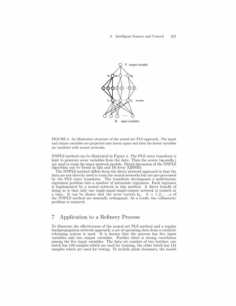
8. Intelligent Sensors and Control 221
........
...
s s ss
X
y
input variables
output variable
s s s...
...
t 2t1 ta
u1 2u ua
scores
FIGURE 4. An illustrative structure of the neural net PLS approach. The inputand output variables are projected onto latent space and then the latent variablesare modeled with neural networks.
NNPLS method can be illustrated in Figure 4. The PLS outer transform iskept to generate score variables from the data. Then the scores (uhandth)are used to train the inner network models. Detail discussion of the NNPLSalgorithm can be found in Qin and McAvoy [QM92b].
The NNPLS method differs from the direct network approach in that thedata are not directly used to train the neural networks but are pre-processedby the PLS outer transform. The transform decomposes a multivariateregression problem into a number of univariate regressors. Each regressoris implemented by a neural network in this method. A direct benefit ofdoing so is that only one single-input-single-output network is trained ata time. It can be shown that the score vectors th, h = 1, 2, . . . , a ofthe NNPLS method are mutually orthogonal. As a result, the collinearityproblem is removed.
7 Application to a Refinery Process
To illustrate the effectiveness of the neural net PLS method and a regularbackpropagation network approach, a set of operating data from a catalyticreforming system is used. It is known that the process has five inputvariables and two output variables. Further there is strong correlationamong the five input variables. The data set consists of two batches, onebatch has 149 samples which are used for training, the other batch has 141samples which are used for testing. To include plant dynamics, the model

222 S. Joe Qin
Training RMSE Testing RMSENNPLS 0.661 0.883
Neural Network 0.663 1.39
TABLE 1. Training and testing root-mean-square errors (RMSE) for a catalyticreformer using the NNPLS method and the neural network approach.
uses several past output values and past input values, that is,
y(t) = f (y(t − 1),y(t − 2), . . . ,y(t − ny),u(t),u(t − 1), . . . ,u(t − nu))(27)
The catalytic reformer data are modeled using the NNPLS approach. Itis found that the time-lags ny = 1 and nu = 1 are good choices for this ap-plication. It is also found with test set validation that seven factors give thebest prediction. The training and test root-mean-square-errors (RMSE’s)are given in Table 1. For comparison, the neural network approach withgradient based training is applied to the same data set. The neural networkhas one sigmoidal hidden layer and the output layer is linear. Under thesame condition as in the NNPLS approach, the training error and the testerror from back-propagation are listed in Table 1. It can be seen that al-though both approaches give similar training results, the NNPLS approachhas better generalization results on the test data. The reason is that theneural net PLS approach is able to reduce variance by removing collinearityin the input data.
8 Conclusions and Recommendations
Owing to the availability of vast amount of historical process data, neuralnetworks have great potential in building models for process quality predic-tion and control. The use of neural networks as intelligent soft sensors canpredict process variables that are not on-line measurable. An immediatebenefit of this application is to have a timely estimation of process qualitywith a cost-effective approach, which allows early control of the processquality if it does not meet the requirement.
When the process data are usually highly correlated, a regular backprop-agation training can result in large prediction variance under correlated in-puts. This large prediction variance causes a large prediction mean-square-error. Several approaches to integrating neural networks with biased sta-tistical methods, including ridge regression, principal component analysis,and partial least squares seem to be able to reduce the mean-square-error.
While there are many training algorithms available, several practical is-sues before and after training a neural network are most time-consumingand deserve further study. Data pre-processing that includes outlier detec-tion and missing value replacement is a typical problem in real applications.Advanced solutions are needed besides check lower-upper bounds for out-liers and interpolations for missing values. Since this topic has been longstudied in statistics, it seems to be beneficial to combine the results instatistics with neural network training.
The issue of variable selection is very important to build a parsimoniousneural network that gives minimal prediction errors. The sensitivity anal-ysis approach discussed is adequate to calculate the relative significance of

8. Intelligent Sensors and Control 223
each input variable with associated time-delay. A further issue is to deter-mine the criteria for selecting or deleting a variable. The cross-validationapproach seems to be effective, but it can be quite time-consuming. Alter-native approaches that could quantify a variable’s contribution against itscontributed variance would be desirable for variable selection.
After a neural network is trained and used for prediction, it is requiredto check the validity of the predicted values. It is important to alert theoperator if a prediction is not valid. Checking the lower and upper boundsfor a variable is necessary, but not sufficient to identify valid regions, partic-ularly when the input variables are highly correlated. Any control actionsbased on the trained neural network should also be conducted within thevalid region.
The use of neural networks as intelligent sensors seems to be a rathergeneral application across various process industries. To build successfulapplications, one need to use several techniques to handle the practicalissues. Therefore, it is worthwhile to study how to package these techniquesin a single software package for process engineers. Although there are manycommercial neural network training package available, most of them placeemphasis on training algorithms but little attention to pre-processing andpost-validation. An easy-to-use toolkit that has comprehensive features toaddress the practical issues could significantly reduce the gap between theacademic research and real-world applications and thus could prevent anypotential misuse of the neural network technology.
9 References[BMMW90] N.V. Bhat, P.A. Minderman, T.J. McAvoy, and N.S. Wang.
Modeling chemical process systems via neural computation.IEEE Control Systems Magazine, pages 24–30, 1990.
[Cyb89] G. Cybenko. Approximation by superpositions of a sigmoidalfunction. Math. of Controls, Signals and Syst., 2:303–314,1989.
[DM94] D. Dong and T.J. McAvoy. Nonlinear principal componentanalysis — based on principal curves and neural networks. InProc. American Control Conference, pages 1284–1288, June29 - July 1, Baltimore, MD 1994.
[DMT+92] B. Dayal, J.F. MacGregor, P. Taylor, R. Kildaw, and S. Marci-kic. Application of artificial neural networks and partial leastsquares regression for modeling kappa number in a continuousKamyr digester. In Proc. of “Control Systems – Dreams vs.Reality”, pages 191–196, 1992.
[GK86] P. Geladi and B.R. Kowalski. Partial least-squares regression:a tutorial. Analyt. Chim. Acta, 185:1–17, 1986.
[HA90] E. Hernandez and Y. Arkun. Neural network modeling andextended DMC algorithm to control nonlinear systems. InProc. American Control Conference, pages 2454–2459, 1990.
[HH92] J.C. Hoskins and D.M. Himmelblau. Process control via arti-ficial neural networks and reinforcement learning. Computersand Chemical Engineering, 16:241–251, 1992.

224 S. Joe Qin
[Hoc76] R.R. Hocking. The analysis and selection of variables in linearregression. Biometrics, 32:1–49, 1976.
[Hoe70] A.E. Hoerl. Ridge regression: biased estimation for non-orthogonal problems. Technometrics, 12:55–67, 1970.
[HSW89] K. Hornik, M. Stinchcombe, and H. White. Multilayer feed-forward neural networks are universal approximators. NeuralNetworks, 2:359–366, 1989.
[Jol86] I. T. Jolliffe. Principal Component Analysis. Springer-Verlag,New York, 1986.
[Kos92] B. Kosko. Neural Networks and Fuzzy Systems. Prentice-Hall,Englewood Cliffs, New Jersey, 1992.
[Kra92] M.A. Kramer. Autoassociative neural networks. Computersand Chemical Engineering, 16:313–328, 1992.
[M+89] T.J. McAvoy et al. Interpreting biosensor data via backprop-agation. In Proc. of Int. Joint Conf. on Neural Networks,volume 1, pages 227–233, Washington, D.C., 1989.
[MMK+91] J.F. MacGregor, T.E. Marlin, J.V. Kresta, et al. Some com-ments on neural networks and other empirical modeling meth-ods. In Proc. of the Chemical Process Control-IV Conference,South Padre Island, TX, Feb. 18–22 1991.
[MN89] H. Martens and T. Naes. Multivariate Calibration. J. Wiley,New York, 1989.
[NP90] K.S. Narendra and K. Parthasarathy. Identification and con-trol of dynamic systems using neural networks. IEEE Trans.on Neural Networks, 1(1):4–27, 1990.
[PO91] M. Piovoso and A.J. Owens. Sensor data analysis using arti-ficial neural networks. In Proc. of Chemical Process Control(CPC-IV), pages 101–118, Padre Island, TX, 1991.
[QM92a] S.J. Qin and T.J. McAvoy. A data-based process modelingapproach and its applications. In Preprints of the 3rd IFACDycord+ Symposium, pages 321–326, College Park, Maryland,April 26–29 1992.
[QM92b] S.J. Qin and T.J. McAvoy. Nonlinear PLS modeling us-ing neural networks. Computers and Chemical Engineering,16(4):379–391, 1992.
[RHW86] D. Rumelhart, G. Hinton, and R. Williams. Learning inter-nal representations by error propagation. In D. Rumelhartand J.L. McClelland, editors, Parallel Distributed Processing,pages 318–362. MIT Press, Cambridge, MA, 1986.
[UPK90] L. Ungar, B. Powell, and E.N. Kamens. Adaptive networksfor fault diagnosis and process control. Comp. and Chem.Engineering, 14:561–572, 1990.

8. Intelligent Sensors and Control 225
[VVY90] Venkatasubramanian. V., R. Vaidyanathan, and Y. Ya-mamoto. Process fault detection and diagnosis using neuralnetworks–I. steady state processes. Comp. and Chem. Engi-neering, 14:699–712, 1990.
[WDM+91] M.J. Willis, C. DiMassimo, G.A. Montague, M.T. Tham, andJ. Morris. Artificial neural networks in processing engineering.Proc. IEE, Part D, 138(3):256–266, 1991.
[WEG87] S. Wold, K. Esbensen, and P. Geladi. Principal componentanalysis. Chemometrics and Intell. Lab. Systems, 2:37–52,1987.
[Wis91] B.M. Wise. Adapting Multivariate Analysis for Monitoringand Modeling Dynamic Systems. Ph.D. thesis, University ofWashington, Seattle, WA, 1991.

226 S. Joe Qin

9
Approximation ofTime–Optimal Control for anIndustrial Production Plantwith General RegressionNeural Network
Clemens SchaffnerDierk Schroder
ABSTRACT For plants which are characterized by a continuous movingweb of material passing between rollers, the sections are coupled by theweb. To make the web control forces smooth and provide fast response,we approximate a time-optimal control with a General Regression NeuralNetwork; simulation results are shown.
1 Introduction
In the paper, plastics, textile or metal industry there are many plantswhich are characterized by a continuous moving web of material. The webhas to pass various sections of rollers in order to enable the execution ofseveral processing steps. The rollers are driven by electric motors. Allsections of the continuous process are coupled by the web. To achieveproper transport and processing results, the web forces have to be keptwithin close limits. Therefore, the electrical and mechanical quantitiesof the drives (e. g. currents, torques, web speeds, web forces) have to becontrolled by closed loop control.
Today most of such plants are equipped with current and speed closedloop control in cascaded structure. The web forces are controlled onlyindirectly in an open loop via the speed relations of neighboring rollers.This control concept suffers from known limitations of cascaded controlstructures.
An important improvement was the development of several linear statespace control concepts, which increased the control quality considerably[WS87]. However, it is impossible to incorporate restrictions on controlvariables in linear design procedures, because they represent nonlinearities.Since restrictions are unavoidable in practical applications, it is desirableto take them into account directly. The control behavior should be as goodas possible with adherence to all restrictions.
These objectives can be met best with an approximation of time-optimalcontrol. Classical time-optimal control laws have some severe drawbacks;the most important one is that they lead to switching controllers, which are

228 Clemens Schaffner , Dierk Schroder
unwinder upwinder
nip–sections
FIGURE 1. Plant
likely to excite unmodeled high-frequency dynamics (see e. g. [PBGM62],[Pap91], [AF66], [BH75], [Fan66], [Kir70]). The resulting oscillations pre-vent stationary accuracy, stress the mechanical and electrical componentsof the plant and can— in extreme cases— destroy parts of the plant. Forthis reason an approximation of the time-optimum with a smooth controlsurface is desirable. Radial basis networks provide smooth output functionsand are therefore well suited. Because of its favorable approximation prop-erties we use a special type of radial basis network, the General RegressionNeural Network (GRNN).
The problem is to create a GRNN so that the plant is controlled in anapproximate time-optimal manner. This is the topic of the paper and isdescribed in detail below.
The paper is organized as follows: In section 2 and 3 we give a briefdescription of the models used for the industrial production plant and theinduction motor drive, respectively. The properties of GRNNs are discussedin section 4. The most important section is section 5 where the consider-ations are described in order to obtain a neural control concept approxi-mating time-optimal control for the plant. Simulation results demonstratethe feasibility of the approach. Final remarks are given in the conclusion.
2 Description of the Plant
A scheme of the considered industrial production plant is depicted in figure1. Such plants with continuous moving webs of material are driven bya large number of electric motors and thus are— from a control pointof view— complex, highly coupled multiple-input/multiple-output systems(MIMO systems).
The winders serve as material storage devices. The web moves with highspeed from the unwinder through a large number of nip-sections (in figure1 there are only 3 nip-sections shown) to the upwinder. In every nip-sectiona processing step is executed; for example the material is dried, deformed,polished, coated, printed, colored, etc. Every section is equipped with aninduction motor drive.
In this paper we assume ideal working conditions for the nip-section next

9. Approximation of Time-Optimal Control 229
ε
ε
εn
FIGURE 2. Signal flow graph of a nip-section
to the unwinder, which means in particular that this nip-section takes overthe function of the leading drive and impresses the nominal web velocity.The following nip-sections are numbered starting from one. The upwinderis controlled ideally so that the web is stored with a given constant webforce, by which the upwinder is decoupled from the last section. We shallinvestigate the dynamic and static behavior of the nip-sections between theleading drive and the upwinder.
In order to give an idea of the physics we want to discuss briefly thesignal flow in a nip-section, for example the third section. With the aboveassumptions the normalized and linearized signal flow graph of this nip-section is depicted in figure 2 ([WS87], [WS93]). To this section belongthe reference value of the motor torque m3soll, the actual motor torquem3, the web velocity v3 at the third roller and the web force f23 betweenthe second and the third roller. IMD (Induction Motor Drive) denotes anonlinear numerical model for an induction motor drive including a voltagesource inverter and torque control, see section 3. The torque m3 of theIMD acts on the integrator with the time constant Tm representing the

230 Clemens Schaffner , Dierk Schroder
combined inertia of the roller and the motor. The difference of the velocityof the second and the third roller v3−v2 produces a strain ε23 via the timeconstant Tb of the web. The factor v0 is the average transport velocityof the web under steady state conditions. The web force f23 is producedby ε23 according to Hooke’s law, expressed through the factor 1
εn. The
difference f34 − f23 gives the reaction of the web to the third roller andthus to the corresponding motor shaft1.
The variables that are to be kept within close limits and have to becontrolled with closed loop control are the web forces f23, f34, f45, f56 andf67 of five coupled nip-sections2. The control variables are the referencevalues of the motor torques m3soll, m4soll, m5soll, m6soll and m7soll. Allquantities are deviations from steady state conditions.
In this paper the following normalized plant parameters are used:
cvi = 1 i = 3 . . . 7εn = 0,005333v0 = 1Ti = 0,00384 s i = 3 . . . 7Tmi = 0,415 s i = 3 . . . 7Tb = 0.4875 s
3 Model of the Induction Motor Drive
In this paper a nonlinear model for the induction motor drives is used forthe numerical simulations. The drives are equipped with a voltage sourceinverter and are torque controlled via closed loop control. It is not thetopic of this paper to describe this model in detail. Nevertheless we wantto give a basic idea of its behavior.
A typical time plot of step responses obtained from an experimental set-up of a modern induction motor drive is depicted in figure 3 [Hin93] Theupper half of the figure shows the reference value of the torque; the lowerpart shows the actual motor torque. Obviously, these transients are quitedifferent from the often used PT1–approximation.
The numerical model is based on [Hin93] and was developed in order todescribe typical stationary and transient phenomena for torque controlledinduction motor drives in a single-phase model:
• During steady state conditions— this means the reference value ofthe torque is constant— the actual torque shows ripples because ofthe switching behavior of the voltage source inverter.
• During transients the gradient of the torque is approximately con-stant. The value of the gradient varies within certain limits accordingto the speed and internal quantities of the drive.
1Please note that all signals throughout this paper are normalized quantities as itis usually done in control engineering. This means all signals are without dimension.The basics of the normalization technique can be found in every introductory controlengineering book.
2The signal flow graph of the coupled system will be shown in section 5.6, figure 19.

9. Approximation of Time-Optimal Control 231
0
M
1Q*
Minenn
Minenn
MM
0
0
-20
40
20
-40
[A]
[A]
M
i
0
0
II
t
t
1Q*
i
t
t
2ms2ms
FIGURE 3. Time plots of the reference torque (top) and of the actual torque(bottom) of an experimental set-up of an induction motor drive equipped with avoltage source inverter
Time plots of step responses obtained from simulations of the numericalmodel are depicted in figure 4 and show good congruence to the experi-mental results of figure 3.
4 General Regression Neural Network
Neural Networks are universal approximators for multi-dimensional nonlin-ear static functions. A neural network can be interpreted as a box, whoseoutputs depend on the specific inputs and on the values of the internal ad-justable weights. This approximation ability is necessary for the proposedcontrol concept. We shall show in section 5 how to generate data which isused as input data for the neural network.
The different types of neural networks differ in their intra— and extrap-olation behavior. In this paper the General Regression Neural Network(GRNN) is chosen because it provides a smooth output function even withsparse data and because its interpolation behavior is predictable [Spe91],[MD89]. These are desirable features especially in closed control loops.The GRNN is a one-pass learning network with a highly parallel structure.The basic idea is similar to the probabilistic neural network, which involvesone-pass learning as well [Spe88].
We want to point out that our control concept does not depend on acertain type of neural network. The control concept can be applied to allneural network paradigms which implement a smooth output function likee. g. the well known backpropagation neural network. However, one dis-advantage of backpropagation is that it needs a large number of iterationsto converge to the desired solution.
The algorithmic form of the GRNN can be used for any regression prob-lem in which an assumption of linearity is not justified. In comparison toconventional regression techniques the GRNN does not need any a-priori

232 Clemens Schaffner , Dierk Schroder
m(t)msoll(t)
t
m(t)msoll(t)
t
FIGURE 4. Simulation results of the numerical model of the induction motordrive equipped with a voltage source inverter: Time plots of the reference torquemsoll(t) (thick line) and of the actual torque m(t) (thin line)
information about the form of the regression functions. It can be imple-mented in parallel hardware or computed in a parallel manner for instanceon transputers. However, sequential software simulation of GRNNs requiressubstantial computation.
The basic equation for a GRNN with m inputs (x = [x1 x2 . . . xm]T )and one output (y is scalar) is
y = y(x) =
p∑ν=1
ϑν · exp(−Cν
σ
)
p∑ν=1
exp(−Cν
σ
) = ϑT · w(x) (1)
where
Cν =m∑
n=1
|xn − χνn|
σ = smoothing parameter
The pairs χν = [χν1 χν
2 . . . χνm]T and ϑν are the data points, which deter-
mine the approximation surface.The output y(x) can be considered as a weighted average of all data
points ϑν(χν) where each data point is weighted exponentially according

9. Approximation of Time-Optimal Control 233
to the Manhattan-distance3 from x. When the smoothing parameter σ ismade very large the output function y(x) is forced to be smooth. As σgoes to 0 y(x) assumes the value of the ϑν(χν) associated with the datapoint closest to x. For intermediate values of σ the data points closer to xare given heavier weight then those further away.
x1
−χ11
x2
−χ12
xm
−χ1m
x1
−χp1
x2
−χp2
xm
−χpm
− 1σ
− 1
σ
− 1
σ
− 1σ
− 1
σ
− 1
σ
ϑ1
numerator of (1)
ϑp
denominator of (1)
output layer
hidden layer
input layer
FIGURE 5. General Regression Neural Network with neural hardware imple-mentation
A neural hardware implementation of a GRNN is depicted in figure 5.The network consists of three layers. In the input layer the components ofthe Manhattan distances |xn − χν
n| are computed. Note that the χνn are
constant because they are part of the data points. The activation functionsof the neurons in the input layer are all identical; they are the absolutevalue function. The outputs of the input layer are amplified by the factors− 1
σ of the synaptic weights in order to provide the corresponding −Cν
σ asinputs for the neurons in the hidden layer. The activation function of allneurons in the hidden layer is the exponential function for the calculation ofexp(−Cν
σ ). The numerator of (1) is constructed by the ϑν–weighted sum ofthe outputs of the hidden layer. The denominator of (1) is simply the sumof all hidden layer outputs. The final division to obtain y has to be doneoutside the GRNN. Extremely fast neural network hardware is availableon the market to implement the GRNN, see e. g. [FHS91]. We illustratethe approximation behavior through a simple 2-dimensional example. The
3Other distance measures, such as e. g. the euclidean distance, are suitable as well.

234 Clemens Schaffner , Dierk Schroder
a) b)
FIGURE 6. Approximation of the XOR-problem on the unit-square. a) σ = 0.2,b) σ = 1.0
data points are
(χν , ϑν)∣∣∣ ν = 1, 2, 3, 4
=([
00
], 1)
,
([01
], 0)
,
([10
], 0)
,
([00
], 1)
which represent the XOR-problem on the unit square. The result of equa-tion (1) with m = 2 and p = 4 is shown in figure 6. There is no over- orundershooting because the output y is bounded by the minimum and themaximum of the ϑν , ν = 1, . . . , p. The output does not converge to poorsolutions corresponding to local minima of an error criterion as it some-times happens with iterative techniques. Furthermore the GRNN allowsone-pass learning (however at the cost of an increasing number of neurons);therefore the learning procedure is very fast. These are— in this context—the main advantages relative to other nonlinear regression schemes, e. g.the well known backpropagation neural network, whose approximation be-havior is unpredictable in principle and which needs an iterative trainingprocedure.
The only parameter which has to be adjusted according to the data set isthe smoothing parameter σ. The simplest method to obtain an appropriateσ is to carry out a few trial-and-error steps, which in our case can be doneeasily with the help of visualization tools.
5 Control Concept
5.1 Some Preliminary Remarks about Time–Optimal Control
Controller design for coupled Multi-Input/Multi-Output (MIMO) systemscan be carried out easily for linear plants with well known linear design

9. Approximation of Time-Optimal Control 235
d m 3 s o l l
d t m a x
m 3 s o l lm a x
≈
d m 3 s o l l
d t m a x
m 3 s o l l m a x
≈
FIGURE 7. Simplification of induction motor drive
techniques, e. g. pole placement. The resulting large matrices can be han-dled by modern high-end CPUs. However, from a practical point of viewthere are some severe drawbacks. A correspondence between system be-havior and specific matrix elements often does not exist. Putting the plantinto operation is a very difficult task. A change of system structure, causedfor instance by a web tear, can result in completely unpredictable and in-definable system reactions.
Furthermore it is impossible to take into account nonlinearities in thelinear controller design procedure. Important nonlinearities are the restric-tions on the motor torque due to indextorque, motorvoltage source inverterphysics and limited power of the induction motor drive. In this paper anonlinear control technique is developed which takes these restrictions intoaccount directly. The aim is to achieve time-optimal control behavior withadherence to the restrictions.
In general time-optimal control means to drive a system from any initialstate into any reference state in the shortest time possible. This task canbe standardized by a linear transformation so that one has to consider onlythe trajectories leading to the origin of the state space.
Often time-optimal control is designed with a single restriction only;namely the limitation of the maximum absolute value of the control vari-able. Under this circumstance the time optimal control obtained is anideal two-point switch. The zero-trajectory serves as switching curve. Zero-trajectories are defined as trajectories which lead to the origin of the statespace while the controller output equals either the positive or the negativemaximum value. It is well-known that this type of time-optimal controlresults in chattering system behavior. Under stationary conditions we ob-serve the characteristic limit cycles, because the controller output switchespermanently between both maximum values.
Our control concept not only avoids these limit cycles but also takes therestriction of the maximum gradient of motor torque changes into account.
5.2 System Trajectories of an Isolated Nip-Section
In order to provide

236 Clemens Schaffner , Dierk Schroder
• a transparent design procedure,
• predictable system behavior in the case of structure changes,
• the opportunity to put the plant into operation sectionwise and
• to achieve a good approximation of time optimal control
we first consider the controller design for an isolated nip-section of loworder. As a representative we consider the third section, which correspondsto the control variable m3soll(t), the actual torque m3(t), the web velocityv3(t) and the web force f23(t). After a controller for such a subsection isfound we shall extend the control concept in order to handle the completecomplex MIMO-system consisting of five coupled nip-sections.
An important idea of our control concept is to introduce restrictions suchthat the actual motor torque is just able to follow the reference value ofthe motor torque with reasonable accuracy. Considering the figures 3 and4 we conclude that if we restrict the reference value of the torque as follows
• the absolute value of m3soll(t) does not exceed a maximum
|m3soll(t)| < |m3soll|max∀t |m3soll|max
= constant (2)
• the absolute value of the time derivative m3soll(t) does not exceed amaximum
|m3soll(t)| < |m3soll|max∀t |m3soll|max
= constant (3)
then — provided the constant values |m3soll|Max and |m3soll|Max are cho-sen appropriately— it is guaranteed that we take nearly full advantage ofthe dynamic capabilities of the induction motor drive while m3 ≈ m3soll;see figure 7. Note that introducing the restrictions (2) and (3) is artificialand thus can be seen as part of the controller. The resulting signal flowgraph for the third isolated nip-section is shown in figure 8. Another ad-vantage resulting from the restrictions (2) and (3) is that now we know themaximum values of the actual torque and its gradient which is importantfor decoupling measures; see section 5.6. The maximum gradient woulddepend otherwise on the speed and on internal quantities of the IMD.
Consequently an important simplification can be made. If we guaranteethat the controller output pays attention to (2) and (3) then it is sufficientto consider two states of the subsystem: the web velocity v3 and the webforce f23. The internal states of the induction motor drive can be neglected.This enables us to use in later sections the control surface with the threedimensions v3, f23 and m3soll as a visualization tool for our considerations.
The two restrictions (2) and (3) imply that there is no analytical solutionpossible for the time-optimal controller. Therefore the controller has to bedesigned by some other means.
In principle the time-plots of time-optimal control trajectories have tolook like the transient in figure 9. Note that the transient is constructedsuch that the restrictions are just not violated. It is sufficient to considertwo switching times, t1 and t2. Starting with t = 0 the control variablem3soll(t) has to be set to the maximum value as fast as possible; thereforethe restriction (3) is active. When the maximum value is reached the

9. Approximation of Time-Optimal Control 237
≈
d m 3 s o l l
d t m a x
m 3 s o l l m a x
ε
ε
εn
FIGURE 8. Signal flow graph of the third isolated nip-section with restrictions
restriction (2) becomes active. At the first switching time t1 the controlvariable has to be decreased with maximum velocity (again restriction (3)is active) until the maximum negative value is reached (again restriction(2) becomes active). After the second switching time t2 the control variablehas to be reduced to zero as fast as possible and after that the transientis completed. We should point out the possibility that the switching timeoccurs before the corresponding maximum value is reached; an example ofthis effect will be given with the simulation results.
As already mentioned before it is the purpose of a transient like the oneshown in figure 9 to drive the system from any initial state into the origin ofthe state space in the shortest time possible. A specific combination of theswitching times t1 and t2 corresponds to a certain initial state. However,this initial state is unknown. On the other hand the final state is known,namely the origin of the state space: web velocity v3 = 0 and web forcef23 = 0.
For this reason we integrate the system backwards in time. We start inthe origin of the state space and use control transients of the type depictedin figure 9 in order to obtain time-optimal system trajectories. We dothis repeatedly with different switching times t1 and t2 in order to generatetime-optimal trajectories distributed over the entire state space. A selection

238 Clemens Schaffner , Dierk Schroder
m3
soll
(t)
|m3 soll|Max
|m3 soll|Max.
t
t
t1
20
FIGURE 9. Typical time-optimal transient m3soll(t)
FIGURE 10. Time-optimal trajectories in the state space
of six trajectories is shown in figure 10. In the meantime we store thecorresponding values of the velocity v3(tν), the web force f23(tν) and thereference torque m3soll(tν) at time instants tν :
χν =[
v3(tν)f23(tν)
]and ϑν = m3soll(tν) for ν = 1, . . . , p (4)
It is the basic idea of our control concept that this data can be used asinput data for a GRNN. The resulting control surface, implemented witha GRNN, will be shown in section 5.5, where the simulation results arepresented.

9. Approximation of Time-Optimal Control 239
web forcef23
web velocity v3
phase planeΩin: linear controller
Ωtrans: combination of
linear controller and GRNN
Ωout: GRNN as neural controller
Ωin
Ωtrans
Ωout
FIGURE 11. Regions in the state space
5.3 Linear-Integral Controller in a Small Region around theStationary State
In order to provide a smooth control surface and to guarantee stationaryaccuracy in the presence of disturbances the state space is divided into threeregions (figure 11): The first region Ωin comprises a small area around thestationary state (which corresponds to the origin of the phase plane of figure11), where only a conventional linear state controller with an integratoris active; the second region Ωtrans is a small layer around Ωin, where asmooth transition between the linear state controller and the nonlinearneural controller is provided; and the third region Ωout comprises the restof the state space, where only the neural controller is used.
The linear controller does not match the demand for time-optimality, butits sphere of activity is so small that it hardly deteriorates the transients.On the other hand the linear controller has some substantial advantages:Because of the integrator the system shows a certain degree of robustnessagainst disturbances; the parameters of the linear controller can be opti-mized with respect to good disturbance rejection. Furthermore no limitcycles around the stationary state occur.
5.4 Approximation of Time-Optimal Control for an IsolatedNip-Section
In section 5.2 we have assumed transitions from any initial state to theorigin of the state space. Now we want to allow arbitrary states as tar-get states. Therefore a linear transformation on the controller has to beperformed. Controller inputs are then the differences m3d, v3d and f23dbetween the actual and the corresponding reference states, which are com-

240 Clemens Schaffner , Dierk Schroder
puted as follows:
m3d = f23soll − m3 (5)v3d = v3 − f23soll · εn · v0 (6)
f23d = f23soll − f23 (7)
To the controller output we have to add the reference value of the webforce f23soll. It is simple to verify this transformation through stationaryconsiderations. As we have already mentioned note that all signals arenormalized quantities.
The resulting controller structure approximating time-optimal control isdepicted in figure 12. It is assumed that all system states are measurablewith negligible time delay. The reference value is the web force f23soll; thecontrolled value is the actual web force f23.
5.5 Simulation Results for an Isolated Nip-Section
Numerical simulations have been done for the control structure of figure12. We applied a step function of the reference value of the web force:
f23soll(t) = 0 for t < 0f23soll(t) = 1 for t ≥ 0
The simulation results are shown in the figures 13— 16. The controlleroutput m3soll(t), figure 13, does not violate the two restrictions (2) and(3); for example:
|m3soll(t)| < 3|m3soll(t)| < 20s−1
The transient of the actual motor torque m3(t), figure 14, shows very clearlythe ripple on the torque because of the switching behavior of the voltagesource inverter4. The time plots of the web velocity v3(t), figure 15, andof the actual web force f23(t), figure 16, show very good approximation ofthe time-optimum. The slight overshoot of f23(t) is caused by the linearcontroller in Ωin.
The resulting control surface, implemented with a GRNN, together witha typical system trajectory is depicted in figure 17.
5.6 Approximation of Time-Optimal Control for theIndustrial Production Plant
We want to use now the results from the previous sections to control thecomplex plant with five highly coupled nip-sections.
In order to maintain the very good approximation of time-optimality itis necessary to introduce some decoupling measures. It is not the topic ofthis paper to discuss decoupling techniques in detail. There are quite a lot
4The simulation was done with the IMD-model; see figure 7 left.

9. Approximation of Time-Optimal Control 241
of different techniques possible; in this paper a relatively simple extensionto the control concept developed so far is chosen. The resulting controlconcept is shown in figures 18 and 19.
For the decoupling in the opposite moving direction of the web the signalpath a (see figure 18) is added which compensates the influence of the webforce f56 of the following nip-section, see figure 19. For the decoupling inthe moving direction of the web the signal b is generated as the weightedsum of the web forces of all preceding nip-sections.
This decoupling measure has to be realized for each nip-section as it isdepicted in figure 19. Because of limited space the control structure of eachsection is summarized by a nonlinear block marked with state/GRNN. Thisblock contains the linear-integral state controller and the GRNN controlleras well as the device for the generation of the correct final controller outputaccording to the description in section 5.3.
5.7 Simulation Results for the Industrial Production Plant
The control system of figure 19 was simulated numerically. We applied astep function of the reference value of the web force of the third section:
f23soll(t) = 0 for t < 0f23soll(t) = 1 for t ≥ 0
The transients of all web forces— f23(t), f34(t), f45(t), f56(t) and f67(t) —are depicted in figure 20.
We applied a step function of the reference value of the web force of theseventh section as well:
f67soll(t) = 0 for t < 0f67soll(t) = 1 for t ≥ 0
The transients of all web forces are shown for this case in figure 21.Figure 20 as well as figure 21 show that the very good approximation of
time-optimality is maintained for the MIMO-case. The transients of f23(t)in figure 20 and of f67(t) in figure 21 are nearly the same as in section 5.5where the time-optimal control for an isolated nip-section was considered.
6 Conclusion
All results and experiences with linear state control concepts for industrialplants of the type described in section 2 show that there is a crucial ob-jective conflict: Either the control parameters are adjusted such that thedecoupling works well but at the expense of a rather bad dynamical be-havior or the other way round [WS93]. Acceptable compromises have tobe found.
It is our belief that via the incorporation of nonlinear control strategiesit is possible to soften this objective conflict, which means to find bettercompromises than it is ever possible with linear techniques.
In this context we have developed a nonlinear control concept. Theuse of neural networks was motivated by the fact that they can represent

242 Clemens Schaffner , Dierk Schroder
arbitrary nonlinear static functions. In this paper we have chosen theGeneral Regression Neural Network because of its favorable approximationproperties.
We have demonstrated how to gain data for the neural network in orderto achieve a control hypersurface which approximates time-optimal con-trol. Simulation results have been presented for an isolated nip-sectionof the plant and the entire complex industrial production plant with fivenip-sections. We have demonstrated that our neural control concept ap-proximates the time-optimum very well. Note that the data acquisitiondescribed in section 5.2 depends on the system parameters. However, inthe described type of industrial production plant there are some parame-ters which vary considerably during operation, for example the proportionalfactor en between the web force and the strain. Therefore it is necessary toadapt the control surface according to these parameter changes. For thispurpose error signals have to be generated and a stable learning law has tobe derived in order to incorporate adaptivity in our control concept. Fur-ther research work will show whether very promising approaches for stableonline learning [SSL95] [SS95] [Sch96] can be used.
7 References[AF66] M. Athans and P.L. Falb. Optimal Control. McGraw–Hill,
1966.
[BH75] A.E. Bryson and Y.-C. Ho. Applied Optimal Control. J. Wiley,1975.
[Fan66] L.-T. Fan. The Continuous Maximum Principle. J. Wiley,1966.
[FHS91] W.A. Fisher, R.J. Hashimoto, and R.C. Smithson. A pro-grammable neural network processor. IEEE Trans. Neural Net-works, 2(2):222–229, March 1991.
[Hin93] D. Hintze. A single–phase numerical model for induction motordrives. Internal report, Institute for Electrical Drives, Techni-cal University of Munich, 1993.
[Kir70] D.E. Kirk. Optimal Control Theory, An Introduction. PrenticeHall, 1970.
[MD89] J. Moody and C.J. Darken. Fast learning in networks oflocally–tuned processing units. Neural Computation, 1(2):281–294, 1989.
[Pap91] M. Papageorgiou. Optimierung. Oldenbourg Verlag, MunchenWien, 1991.
[PBGM62] L.S. Pontryagin, V. Boltyanskii, R. Gamkrelidze, and E. Mis-chenko. The Mathematical Theory of Optimal Processes. In-terscience Publishers, New York, 1962.
[Sch96] C. Schaffner. Analyse und Synthese Neuronaler Regelungsver-fahren. Ph.D. thesis, Herbert Utz Verlag Wissenschaft,Munchen, 1996. ISBN 3–931327–52–3.

9. Approximation of Time-Optimal Control 243
[Spe88] D. Specht. Probabilistic neural networks for classification,mapping or associative memory. In Proc. IEEE Int. Conf. Neu-ral Networks, volume 1, pages 525–532, June 1988.
[Spe91] D. Specht. A general regression neural network. IEEE Trans.Neural Networks, 2(6):568–576, November 1991.
[SS95] C. Schaffner and D. Schroder. Stable nonlinear observer designwith neural network. In IFAC–Workshop on Motion Control,pages 567–574, Munich, Germany, 1995.
[SSL95] C. Schaffner, D. Schroder, and U. Lenz. Application of neuralnetworks to motor control. In International Power ElectronicConference, IPEC 1995, volume 1, pages 46–51, Yokohama,Japan, 1995.
[WS87] W. Wolfermann and D. Schroder. Application of decouplingand state space control in processing machines with continuousmoving webs. In Preprints of the IFAC 1987 World Congresson Automatic Control, volume 3, pages 100–105, 1987.
[WS93] W. Wolfermann and D. Schroder. New decentralized control inprocessing machines with continuous moving webs. In Proceed-ings of the Second International Conference on Web Handling,Stillwater, Oklahoma, June 6–9 1993.

244 Clemens Schaffner , Dierk Schroder
ε
ε
≈
εε
d t m a x
m a x
FIGURE 12. An isolated nip-section with neural control

9. Approximation of Time-Optimal Control 245
FIGURE 13. Time plot of m3soll(t) for a step function of f23soll(t); isolatednip-section
FIGURE 14. Time plot of m3(t) for a step function of f23soll(t); isolatednip-section

246 Clemens Schaffner , Dierk Schroder
t
v3(t)
FIGURE 15. Time plot of v3(t) for a step function of f23soll(t); isolatednip-section
t
f23(t)
FIGURE 16. Time plot of f23(t) for a step function of f23soll(t); isolatednip-section

9. Approximation of Time-Optimal Control 247
web velocity
web force
control variable
3
23
3
v
f
m soll
FIGURE 17. Control surface of the General Regression Neural Network and atypical system trajectory

248 Clemens Schaffner , Dierk Schroder
ε
ε
≈
εε
d t m a x
m a x
ab
FIGURE 18. Signal flow graph of the neural control concept extended by adecoupling measure (signals a and b)

9. Approximation of Time-Optimal Control 249
ε
dt
ma
x
ma
x
ε
dt
ma
x
ma
x
ε
dt
ma
x
ma
x
ε
dt
ma
x
ma
x
dt
ma
x
ma
x
FIGURE 19. Signal flow graph of the neural control concept for the industrialproduction plant extended by decoupling measures

250 Clemens Schaffner , Dierk Schroder
0.00 0.05 0.10 0.15t
f
f
f
f
f
34
45
56 67
23
,
-0.5
0.0
0.5
1.0
1.5
FIGURE 20. Time plot of the web forces f23(t), f34(t), f45(t), f56(t) and f67(t)due to a step function of f23soll(t)
0.00 0.05 0.10 0.15t
f f f f
f
23 34 45 56
67
, , ,
-0.5
0.0
0.5
1.0
1.5
FIGURE 21. Time plot of the web forces f23(t), f34(t), f45(t), f56(t) and f67(t)due to a step function of f67soll(t)

10
Neuro-Control Design:Optimization Aspects
H. Ted SuTariq Samad
ABSTRACT This chapter views neural-network-based control system de-sign as a nonlinear optimization problem. Depending on the role of a neuralnetwork in the system, the neural-control problems are classified into a fewcategories. A unifying framework for neuro-control design is presented toview neural network training as a nonlinear optimization problem. Thisarticle then outlines a new neuro-control concept, referred to as “Parame-terized Neuro-Controller (PNC),” and discusses the optimization complex-ities it poses. To demonstrate the unique characteristics of this new neuralcontrol design concept, simulation results are presented at the end of thisarticle.
1 Introduction
The recent and considerable interest in neuro-control has resulted in anumber of different approaches to using neural networks in control systemdesign. For applications in the process industries, the most relevant ofthese are based on using neural networks as identifiers or optimizing neuralnetwork controllers using a process model. Successful practical applicationsof this approach are now in operation, e.g. [TSSM92, Sta93].
This chapter views neural-network-based control system design as a non-linear optimization problem. Depending on the characteristics of the appli-cation, it also shows how different optimization algorithms may be appro-priate. A fundamental distinction is made between gradient-based and non-gradient-based algorithms. In the former case, a variety of techniques areavailable for gradient computation. Although gradient-based algorithmscan be expected to be significantly more efficient than non-gradient-basedones, there are applications where gradient computation is infeasible. Forexample, desired control performance criteria are not always differentiable,local minima may render strict gradient methods useless, and not all pro-cess models allow analytical derivatives. This article reviews a number ofnon-gradient algorithms that have recently been used in neuro-control.
To illustrate the appropriateness for non-gradient algorithms, this ar-ticle outlines a new neuro-control concept and discusses the optimizationcomplexities it poses. This concept is referred to as “Parameterized Neuro-Controller” (PNC) [SF93]. PNCs designed with two types of external pa-rameters are considered: process parameters that provide the controller

252 H. Ted Su , Tariq Samad
with information regarding the dynamical characteristics of the process(e.g. dead time, gain), and control parameters that indicate characteris-tics of the desired closed-loop behavior (e.g. maximum overshoot, desiredsettling time). These two types of parameters make a PNC a generic con-troller. It is generic in two aspects: 1) a PNC is applicable to differentprocesses, and 2) a PNC is adjustable or tunable for its closed-loop controlperformance.
This article presents simulation results showing the pervasiveness of localminima for this application. The algorithm used in this study integratesthe population-based search of a genetic algorithm with the random-walkaspect of chemotaxis. Experimental results on a low-order model appro-priate for chemical processes are presented.
2 Neuro-Control Systems
This section briefly reviews various approaches in current neuro-controldesign. Although there are other ways to classify these approaches, e.g.[HSZG92], this chapter nevertheless adopts one similar to adaptive controltheory: 1) indirect neuro-control and 2) direct neuro-control.
In the indirect neuro-control scheme, a neural network does not send acontrol signal directly to the process. Instead, a neural network is oftenused as an indirect process characteristics indicator. This indicator canbe a process model which mimics the process behavior, or a controllerauto-tuner which produces appropriate controller settings based upon theprocess behavior. In this category, the neuro-control approaches can beroughly distinguished as follows: 1) neural network model-based control,2) neural network inverse model-based control, and 3) neural network auto-tuner development.
In the direct neuro-control scheme, a neural network is employed as afeedback controller, and it sends control signals directly to the process.Depending on the design concept, the direct neuro-control approaches canbe categorized into: 1) controller modeling, 2) model-free neuro-controldesign, 3) model-based neuro-control design, and 4) robust model-basedneuro-control design.
Regardless of these distinctions, a unifying framework for neuro-controlis to view neural network training as a nonlinear optimization problem:
NN : minw
J(w) (1)
in which one tries to find an optimal representation of the neural networkthat minimizes an objective function J over the network weight space w.Here, NN indicates that the optimization problem formulation involves aneural network. The role a neural network plays in the objective functionis then a key to distinguishing the various neuro-control design approaches.To make this article more interesting, the appearance/formulation of Eqn. 1will take various forms in the discussion to follow. As the main thrust of thisarticle, the optimization aspects of various neuro-control design approachesare discussed based upon the formulation of the objective function. Thevarious optimization problems are not precisely but rather conceptuallyformulated for discussion purposes.

10. Neuro-Control Design 253
Plant
NeuralNetwork
u y
u’
Training
FIGURE 1. Neural network can be used as a black-box model of a process.
2.1 Indirect Neuro-Control
Neural Network Model-Based Control
Full Neural Network ModelThe most popular control system application of neural networks is to use aneural network as an input-output process model. This approach is a datadriven supervised learning approach, i.e., the neural network attempts tomimic an existing process from being exposed to the process data (see Fig.1). The most commonly adopted model structure for such a purpose isthe nonlinear auto-regressive and moving average with exogenous inputs(known as NARMAX) model or a simpler NARX [CBG90, SMW92]. Thisfamily of NARMAX models is a discrete-time nonlinear transfer function[Lju87]. Alternatively, one can choose to identify a continuous-time modelwith a dynamic neural network, e.g. a recurrent network [Wer90].
Regardless of the model structure and the control strategy, the neuro-control design in this case can be conceptually stated as follows:
NN : minw
Fyp − yn(w, ...) (2)
where yp stands for plant/process output, yn for neural network output,and w for neural network weights. Here F· is a functional that measuresthe performance of the optimization process. It is usually an integral orsum of the prediction errors between yp and yn. For example, in this modeldevelopment stage, process inputs and output up, yp are collected over afinite period of time and used for neural network training. F· is usuallyan integral of the 2-norm of yp − yn. A typical example of Eqn. 2 is asfollows:
NN : minw
∑t
|yp(t) − yn(t)|2; yn(t) = N (w, ...) (3)
Once the model is developed, it can then be implemented for model-basedcontrol design.

254 H. Ted Su , Tariq Samad
-+ Plant
yy u
-+
u
u
Constraints
-
+
+
d
+
ModelModel
Optimizer
NLMPC
-
y
y
y
FIGURE 2. A neural network model can be incorporated into nonlinear ModelPredictive Control (MPC) scheme.
At the implementation stage, nevertheless, the neural network modelcannot be used alone. It must be incorporated with a model-based controlscheme. In the chemical process industry, for example, a neural networkis usually employed in a nonlinear model predictive control (MPC) scheme[SM93b, SM93a]. Fig. 2 illustrates the block diagram of an MPC controlsystem. In fact, the MPC control is also an optimization problem. Theoptimization problem here can often be expressed as follows:
minu
F ′y∗ − yn(u, ...) (4)
where y∗ designates the desired closed-loop process output, u the pro-cess/model input or control signal, and yn the predicted process output(by the neural network model). Here F ′ stands for an objective functionthat evaluates the closed-loop performance. For example, the optimizationproblem in the implementation stage is usually as follows:
minu
∑t
|y∗(t) − yn(t) − d(t)|2, yn(t) = N (u, ...) (5)
where y∗(t) stands for desired setpoint trajectory, and d(t) for estimateddisturbance. This optimization is performed repeatedly at each time in-terval during the course of feedback control. Although the constraints arenot particularly of interest in the discussion, one advantage of this indirectcontrol design approach over the direct ones is that the constraints canbe incorporated when solving the above optimization problem. For moredetails about MPC, refer to [SDBM91, SM93b, SM93a] for example.
As discussed later, moreover, a full neural network model can be incorpo-rated into other neuro-control schemes, such as neural network auto-tunerdesign (Section 2.1), model-based controller modeling (Section 2.2), andmodel-based neuro-control design (Section 2.2 and Section 2.2).
Parametric or Partial Neural Network ModelIn some cases, a certain degree of knowledge about the process might beavailable, such as model structure or particular physical phenomena that

10. Neuro-Control Design 255
Plant
NeuralNetwork
u y
y’
Training
Model
Complete model
FIGURE 3. A neural network can be a parameter estimator, model structureselector, or partial elements of a physical model.
are well-understood. In this case, a full black-box model might not be mostdesirable. For example, if the structure of the process model is available,values for the associated parameters can be determined by a neural net-work. Examples of these parameters can be time constants, gains, anddelays or physical parameters such as diffusion rates and heat transfer co-efficients. Psichogios and Ungar [PU92] employed such an approach tomodel a fedbatch bioreactor. Kramer [TK94] also presented an hybridmodel structure that incorporated prior knowledge into neural networkmodels. When model structure is not known a priori, neural networks canbe trained to select elements of a model structure from a predeterminedset [KSF92]. These elements can then be composed into a legal structure.Lastly, in other cases where model structure is partially known, neural net-works can also be integrated with such a partial model so that the processcan be better modeled [SBMM92].
For illustration purpose, the parametric or partial neural network mod-eling problem can be formulated as follows:
NN : minw
Fyp − ym(θ, ...); θ = N (w, ...) (6)
where ym is the predicted output from the model and θ stands for theprocess parameters, model structural information, or other elements re-quired to complete the model. Notice the only difference between Eqn. 6and Eqn. 2 is that ym replace yn. From a model-based control standpoint,this approach is essentially identical to the full black-box neural networkmodel except that the neural network does not directly mimic the processbehavior.
Neural Network Inverse ModelIn this approach, a neural network is trained to develop an inverse modelof the plant. The network input is the process output, and the networkoutput is the corresponding process input (see Fig. 4). In general, theoptimization problem can be formulated as:
NN : minw
Fu∗p−1 − un(w, ...) (7)

256 H. Ted Su , Tariq Samad
Plant
NeuralNetwork
u y
u’
Training
FIGURE 4. A neural network inverse model.
where u∗p−1 is the process inputs. Typically, the inverse model is a steady
state/static model, which can be used for feedforward control. Given adesired process setpoint y∗, the appropriate steady-state control signal u∗for this setpoint can be immediately known:
u∗ = N (y∗, ...) (8)
Successful applications of inverse modeling are discussed in [MMW90] and[SW90]. Obviously, an inverse model exists only when the process behavesmonotonically as a “forward” function at steady state. If not, this approachis inapplicable.
One can also find a few articles addressing a similar “inverse model”concept of using a non-static inverse neural network model for control[BM90, Yds90, UPK90, PU91]. In principle, an inverse neural networkmodel can learn the inverse dynamics under some restrictions (e.g. min-imum phase and causality are required). Then, the inverse model is ar-ranged in a way similar to an MPC controller. In practice, especially fordiscrete-type dynamic models, the inverse model may not be able to learnthe desired inverse dynamics. For example, Psichogios & Ungar [PU91]trained an inverse model and then performed some control case studies.The “inverse model” approach failed to function as expected. In manycases, a process inverse is in fact non-causal even if the process behavesmonotonically as mentioned above. The non-causality of a process inversecan result from transport delay (dead time) or discretization of a continu-ous process in a sampled-data system. Even if an inverse model does exist,the use of a dynamic inverse model as a feedback controller will not resultin a strictly proper control system. Strict properness is essential in controlsystem design [MZ89].
In some of the open literature, “inverse-modeling” is sometimes used torefer to training a neural network “model” in a closed-loop environment,e.g. [HSZG92, PSY88]. This “inverse-modeling” approach does not lead toan “inverse model” that inverts the forward function of the process/plantof interest. For example, the process as a function maps input variablesto output variables, whereas the “inverse model” does not map the sameoutput variables or to the same input variables. Instead, it often maps the

10. Neuro-Control Design 257
Model orProcessu
yr
Training
NeuralNetwork
Controller
FIGURE 5. Closed-Loop neural network auto-tuner.
difference between the output variables and the goal (or set points) to theinput variables. From this paper’s perspective, this approach belongs tothe category of “neuro-control” design, and will be discussed in sections tofollow.
Neural Network Auto-TunerAs in the previous case where neural networks can be used to estimateparameters of a known model, they can also be used to estimate tuningparameters of a controller whose structure is known a priori. A controller’stuning parameter estimator is often referred to as an auto-tuner. Theoptimization problem in this case can be formulated as follows:
NN : minw
Fη∗ − ηn(w, ...) (9)
where η∗ denotes the controller parameters as targets, and ηn stands for thepredicted values by the neural network. Network input can comprise sam-pled process data or features extracted from it. However, these parametersη cannot be uniquely determined from the process characteristics. Theyalso depend on the desired closed-loop control system characteristics. Usu-ally, the controller parameters η∗ are solutions to the following closed-loopcontrol optimization:
minη
F ′y∗ − yp/m(u, ...); u = C(η, ...) (10)
where C is a controller with a known structure. Here, yp/m denotes thateither a process or a model can be employed in this closed-loop control inorder to find the target controller C.
Actually, the attraction of this approach is that the network can betrained in simulation. Training on actual process data is not necessary.For open-loop auto-tuning, an open-loop simulation is sufficient; otherwisea closed-loop simulation is needed (see Fig. 5). The training must be con-ducted over a space of process models. Ideally, this space should cover theprocesses that will be encountered during operation.
Most work to date in auto-tuning is directed at the PID controllersas they are still the most widely used control structure in practice. Ap-propriate values for the PID gains (Kc/proportional gain, Ki/reset time,

258 H. Ted Su , Tariq Samad
Kd/derivative time) are essential if the closed-loop system is to performin a desired manner. PID tuning is still largely a manual procedure of-ten relying on heuristics developed over a half-century ago [ZN42]. Severalauto-tuners are commercially available, but improvements are still needed.For neural-network auto-tuner design, low-order linear models with rangesfor parameters are likely to suffice for most PID applications.
Developments of this concept are discussed by Swiniarski [Swi90] and Ru-ano et al. [RFJ92]. In [Swi90], the network is trained using Ziegler-Nicholsheuristics for determining target PID gains. During operation, the input tothe network is 128 samples of open-loop process step response. Thus the re-sulting auto-tuner requires open-loop operation of the process. In contrast,Ruano et al. describe a method for open-loop or closed-loop auto-tuning,accomplished by preprocessing input/output data. Optimal PID gains fortraining purposes are computed with a quasi-Newton optimization algo-rithm initialized with Ziegler-Nichols values. The optimization criterion isthe minimization of the integral of time-multiplied absolute error (ITAE).The authors show how a closed-loop auto-tuner can effectively adapt PIDparameters on-line in response to setpoint changes for the control loop.
2.2 Direct Neuro-Control
Controller Modeling
Among the four direct neuro-control schemes, the simplest one to neuro-controller development is to use a neural network to model an existingcontroller. The input to the existing controller is the training input tothe network and the controller output serves as the target. In fact, thisapproach is similar to the neural network modeling approach discussed inSection 2.1 except that the target here is not a process but a controller.Likewise, this neuro-control design can be formulated as follows:
NN : minw
Fuc − un(w, ...) (11)
where uc∗ is the output of an existing controller C∗. Usually, the existingcontroller C∗ can be a human operator or it can be obtained via:
minC
F ′y∗ − yp/m(u, ...); u = C(...) (12)
Like a process model, a controller is generally a dynamical system, andoften comprises integrators or differentiators. If an algebraic feed-forwardnetwork is used to model the existing controller, dynamical informationmust be explicitly provided as input to the network. This dynamical in-formation can be provided either as appropriate integrals and derivativesor as tapped delay signals of process data. For example, to model a PIDcontroller, an algebraic neural network needs not only the instantaneouserror between the set-point and the process output, but also the derivativeand integral of the error. Alternatively, one can train a neural network witha series of those errors and/or the controller outputs in the previous timesteps. The latter approach is similar to developing an ARX (auto-regressivewith exogenous inputs) type process model, except that the inputs and theoutputs of the process are replaced with feedback errors and controlleroutputs.

10. Neuro-Control Design 259
Controller
NeuralNetwork
e u
u’
Training
FIGURE 6. The simplest approach to neuro control design is to use a neuralnetwork to model an existing controller
In general, this approach can result in controllers that are faster and/orcheaper than existing controllers. Using this approach, for example, Pomer-leau [Pom91] presented an intriguing application, where a neural networkis used to replace a human operator, i.e. an existing controller. The CMUNavlab van, equipped with a video camera and an imaging laser range-finder, is driven by a human operator at about six miles per hour for aboutfive minutes. During this time, a neural network is trained “on-the-fly” tolearn the mapping from the video and laser range-finder inputs to steer-ing actions. Subsequently, the network can drive the van autonomously atspeeds of up to the maximum of 20 MPH, which is over twice as fast as anyother sensor-based autonomous system has driven the Navlab. Moreover,neural networks have been developed that are capable of driving on single-lane dirt roads, two-lane suburban neighborhood streets, and lined two-lane highways. With other sensory inputs additional capabilities have beenachieved, including collision avoidance and nocturnal navigation. Pottmanand Seborg [PS92] also present a neural network controller that is trainedto learn an existing MPC controller. Given any setpoint change and dis-turbance, the MPC controller uses a neural network model and performson-line optimization to calculate the optimal control signal. The resultingneuro-controller can then replace the “on-line optimizing” MPC and yieldssimilar near-optimal results except the neuro-controller is faster since itdoes not need any on-line optimization.
While the benefits of this approach may be apparent when the existingcontroller is a human, its utility may be limited. It is applicable only whenan existing controller is available, which is the case in many applications.Staib and Staib [SS92] discuss how it can be effective in a multi-stage train-ing process. A neural network is trained to mimic an existing controller,and then further refined in conjunction with a process model—the model-based control design concept to be discussed later.
Model-Free Neuro-ControlIn the absence of an existing controller, some researchers have been inspiredby the way a human operator learns to “control/operate” a process withlittle or no detailed knowledge of the process dynamics. Thus they have

260 H. Ted Su , Tariq Samad
PlantNeuralNetwork
u yr
Training
FIGURE 7. The model-free control design concept.
attempted to design controllers which, by adaptation and learning, cansolve difficult control problems in the absence of process models and humandesign effort. In general, this model-free neuro-control design can be statedas:
NN : minw
Fy∗ − yp(u, ...); u = N (w, ...) (13)
where yp is the output from the plant. The key feature of this directadaptive control approach is that a process model is neither known inadvance nor explicitly developed during control design.
This control design problem is often referred to as “reinforcement learn-ing.” However, this article chooses to refer to this class of control design as“model-free neuro-control design” as it is more appropriate in the contextof the discussion [SF93]. Fig. 7 is a typical representation of this class ofcontrol design.
The first work in this area was the “adaptive critic” algorithm proposedby Barto et al. [BSA83]. Such an algorithm can be seen as an approximateversion of dynamic programming [Wer77, BSW90]. In this work, they poseda well-known cart-pole balancing problem, and demonstrated their designconcept. In this class of control design, limited/poor information is oftenadopted as an indication of performance criteria. For example, the objec-tive in the cart-pole balancing problem is simply to maintain the pole ina near-upright balanced position for as long as possible. The instructionalfeedback is limited to a “failure” signal when the controller fails to hold thepole in an upright position. The cart-pole balancing problem has become apopular test-bed for explorations of the model-free control design concept.
Despite its historical importance and intuitive appeal, model-free adap-tive neuro-control is not appropriate for most real-world applications. Theplant is most likely out-of-control during the learning process, and few in-dustrial processes can tolerate the large number of “failures” needed toadapt the controller.
Model-Based Neuro-ControlFrom a practical perspective, one would prefer to let failures take place ina simulated environment (with a model) rather than in a real plant evenif the failures are not disastrous or do not cause substantial losses. As

10. Neuro-Control Design 261
ModelNeuralNetwork
u yr
Training
FIGURE 8. A model replaces the plant/process in the control system during thecontrol design phase.
opposed to the previous case, this class of neuro-control design is referredto as “model-based neuro-control design.” Similar to Eqn. 13, as a result,the problem formulation becomes:
NN : minw
Fy∗ − ym(u, ...); u = N (w, ...) (14)
Here, yp in Eqn. 13 is replaced by ym—the model’s output. In this case,knowledge about the processes of interest are required. As can be seen inFig. 8, a model replaces the plant/process in the control system (cf. Fig.7).
If a process model is not available, one can first train a second neuralnetwork to model the plant dynamics as discussed in Section 2.1. In thecourse of modeling the plant, the plant must be operated “normally” in-stead of being driven out-of control. After the modeling stage, the modelcan then be used for control design. If a plant model is already available,a neural network controller can then be developed in a simulation in whichfailures cannot cause any loss but that of computer time. A neural networkcontroller after extensive training in the simulation can then be installedin the actual control system.
In fact, these “model-based neuro-control design” approaches have notonly proven effective in several studies [NW90, Tro91], but also have alreadyproduced notable economic benefits [Sta93]. These approaches can be usedfor both off-line control design and for on-line adaptation.
Successful demonstrations have been performed for the “truckbackerup-per” problem [NW90] and a multi-variable flight control problem [TGM92].Perhaps the biggest commercial success of neuro-control to date is alsobased on this approach. The Intelligent Arc FurnaceTM, developed by Neu-ral Applications Corporation and Milltech-HOH, is a product that uses aneural network to regulate electrode position in electric arc furnaces [SS92].A trade publication reports typical savings of over $2 million per furnaceper year [Keh92]. Milltech-HOH and Neural Applications Corporation re-ceived an Outstanding Engineering Achievement Award for 1992 from theNational Society of Professional Engineers.
The Intelligent Arc Furnace controller includes an interesting twist on

262 H. Ted Su , Tariq Samad
ModelModelModelModelModelNeural
Networku yr
Training
FIGURE 9. In robust control design concept, the controller is designed not onlyfor a nominal process but also for a family of processes.
neuro-controller development. Initially, the neural network controller istrained to mimic an existing plant controller (cf. Section 2.2). After train-ing, the neural network then replaces the existing controller. In this latterstage, a second, pre-trained, neural network is used as the process model.Both the process model network and the controller network continue toadapt on-line to compensate for plant drifts.
Nevertheless, the quality of control achieved with this approach dependscrucially on the quality of the process model. If a model is not accurateenough, the trained neuro-controller is unlikely to perform satisfactorily onthe real process. Without an on-line adaptive component, it does not allowfor plant drifts or other factors that could adversely affect the performanceof the control system. A controller that is highly optimized for a specificprocess cannot be expected to tolerate deviations from the nominal processgracefully.
Robust Model-Based Neuro-ControlThe neuro-controller approaches discussed above still share a common short-coming: A neural network must be trained for every new application. Net-work retraining is needed even with small changes in the control criterion,such as the changes on the relative weighting of control energy and track-ing response, or if the controller is to be applied to a different but similarprocess. In order to circumvent such drawbacks, the concept of robust-ness is naturally brought into the design of a neuro-controller. In robustmodel-based neuro-control design, a family of process models is consideredinstead of just a nominal one (see Fig. 9). Often such a family is specifiedby a range of noise models or a range of the process parameters. Robustneuro-control design can be formulated as follows:
NN : minw
Fy∗ − ymi(u, ...);u = N (w, ...), ∀ mi ∈ M (15)
where mi stands the i−th member of the model family M. Ideally, thereal process to be control should belong to this family as well so that thecontroller is robust not only for the model but also for the real process.
Two aspects of robustness are commonly distinguished. Robust stabilityrefers to a control system that is stable over the entire family of process,

10. Neuro-Control Design 263
ModelModelModelModelModelNeural
Networku yr
Process and otherParameterization
Training
FIGURE 10. PNC control design is to design not only a robust but also a genericcontroller.
whereas robust performance refers to performance criteria being satisfiedover the family [MZ89]. Not surprisingly, there is a tradeoff to achieverobustness. By optimizing a neural network controller based upon a fixed(and accurate) process model, high performance can be achieved as longas the process remains invariant, but at the likely cost of brittleness. Arobust design procedure, on the other hand, is not likely to achieve thesame level of nominal performance but will be less sensitive to processdrifts, disturbances, and other sources of process-model mismatch.
2.3 Parameterized Neuro-ControlAll the above neuro-control approaches share a common shortcoming—theneed for extensive application-specific development efforts. Each applica-tion requires the optimization of the neural network controller and may alsorequire process model identification. The expense in time and computa-tion is a significant barrier to widespread implementation of neuro-controlsystems, and compares unfavorably to the cost of implementation for con-ventional control. Simple linear control schemes such as PID controllers,for example, enable the use of one control law in domains as diverse asbuilding, process, and flight control.
In an attempt to avoid application-specific development, a new neuro-control design concept—“Parameterized Neuro-Control (PNC)”—is thenevolved [SF93, SF94]. Fig. 10 illustrates this PNC design strategy. ThePNC controller is equipped with parameters that specifies process charac-teristics and those that provides performance criterion information. Forillustration purpose, a PNC can be conceptually formulated as follows:
NN : minw
F (ξ)y∗ − ymi(θ, u, ...);u = N (w, θ, ξ, ...), ∀ mi(θ) ∈ M(θ)
(16)where ξ designates the parameter set that define the space of performancecriteria, θ stands for the process parameter set, θ is the estimates for processparameters, and again M(θ) is a family of the parameterized models mi(θ)in order to account for errors in process parameters estimates θ.

264 H. Ted Su , Tariq Samad
Proportional Band
Reset Time
Derivative Time
Settling Time
Maximum Overshoot
Others
PID PNC
FIGURE 11. A plausible PNC can be equipped with tunable knobs, such as“Settling Time Knob” or “Maximum Overshoot Knob.” Such a PNC can bemuch easier for an operator to set the tuning parameters in order to achieve adesirable control performance without basic knowledge of control theory.
In fact, the two additional types of parameters (ξ and θ) make a PNCgeneric. A PNC is generic in two perspectives: 1) the process model pa-rameters θ facilitate its application to different processes and 2) the perfor-mance parameters ξ allow its performance characteristics to be adjustableor tunable. For example, if a PNC is designed for first-order plus delayprocesses, the process parameters (i.e. process gain, time constant, anddead time) will be adjustable parameters to this PNC. Once developed,this PNC requires no application-specific training or adaptation when ap-plied to a first order plus delay process. It only requires estimates of theseprocess parameters. These estimates do not have to be accurate becausethe robustness against such inaccuracy is considered in the design phase.Notice that the parameters θ used as input to the PNC is not identical tothe parameter θ used in the process model simulation. Parameters thatspecify the performance criterion can be, for example, the value of maxi-mum allowable overshoots, desired settling times or rise times, or integralabsolute errors when encountering particular setpoint changes or distur-bances. The resulting controller can be featured by a tuning knob that anoperator can easily understand for controlling the process. Using such tun-ing knobs, say a “settling time knob” (see Fig. 11), an operator can set thecontroller so that it makes the process settle faster or slower in the presenceof a disturbance. To do so, the operator does not need any sophisticatedknowledge of control theory or extensive practice. Fig. 11 presents a plau-sible easy-to-use PNC in comparison with a conventional PID controller.The performance criteria such as settling time or maximum overshoot canbe directly tunable by an operator.
3 Optimization Aspects
The previous section has discussed various neuro-control design approaches.This section further addresses the optimization aspects in these neuro-

10. Neuro-Control Design 265
control design problems. For convenience, all the optimization problemsare listed in Table 1. In the second column of the table, “S” indicates aproblem for which simple supervised learning is appropriate; whereas “C”indicates that a closed-loop system is needed in order to solve the associ-ated optimization problem. A closed-loop system consist of a plant or amodel and a feedback controller. It is needed for evaluating the controller’sperformance against the criterion.
As all the neuro-control design strategies require the solution of an op-timization problem, solution techniques become crucial. Depending on thecharacteristics of the application, a particular optimization algorithm mayor may not be appropriate. In particular, gradient-based optimization al-gorithms, which require the availability of Jacobian of J with respect tothe decision variables, are not appropriate for applications involving non-differentiable objective functions. To further address the optimization as-pects of neuro-control design, this section hence discusses two classes ofoptimization algorithms: gradient and non-gradient algorithms.
3.1 Gradient Algorithms
As a universal function approximator, a neural network has a remarkablefeature in providing gradient information. Gradient information of its out-puts with respect to its weights as well as its inputs can be easily calculatedin a localized fashion. Such gradient information can be back-propagatedfrom its outputs through its internal variables (e.g. hidden layers) and thenthe inputs of the network. The well-known back-propagation (BP) algo-rithm [RHW86] is one of the best examples to illustrate this feature. Inthe BP algorithm, all the gradients (Jacobian of J with respect to w) canbe calculated with merely localized information.
Gradient algorithm can be applied to items labeled with ”S” in Table 1.In all indirect neuro-control approaches as well as the controller modelingapproach, the neural network is trained over a set of training data collectedfrom its target. The target is an existing process, or an existing controller.Using the training data, the neural network can then be trained via super-vised training approaches. One key advantage of the supervised learningis that the gradient information, i.e. the Jacobian ∂J/∂w, can be easilycalculated. The analytical Jacobian is available as long as F or F ′ is in adifferentiable form. Often, F takes the form of a 2-norm of its arguments(e.g. Eqn. 3) because of its simple differential form.
In Table 1, neuro-control problems labeled with “C” are in fact typicalformulations of optimal control. These optimal control problems requires aclear mathematical definition of the performance criteria. The optimizationissue in these optimal control problems is in fact typical in the calculus ofvariations [WJ92]. The time-variant characteristics of the decision variables(i.e. states and control signals) make the problem extremely complex. Inoptimal control theory, however, the introduction of “co-state” variablesprovides a substantial reduction of complexity—the optimization problembecomes a two-point boundary value problem. The co-state variables aretime-variant Lagrange multipliers as opposed to those in a time-invariantconstrained optimization problem.
Among all solution techniques to the boundary value problem, the gradi-ent descent algorithm is probably the most straightforward one. Gradientalgorithms are useful as long as the Jacobian with respect to w or u is

266 H. Ted Su , Tariq Samad
computable. A commonly adopted algorithm in neural network training fora dynamic system is “back-propagation through time” [Wer90, SMW92].Unlike the “S” problems listed in Table 1, the availability of an analyticalJacobian (∂F/∂u or ∂F/∂w) requires that ∂yp/∂w or ∂yp/∂u is available(in addition to that F is differentiable).
Of course, the convergence rate of gradient descent can be greatly im-proved with higher-order gradient information, such as the Hessian (sec-ond order). With second-order derivatives, Newton methods can be used.Additionally, Levenberg-Marquardt algorithm provides an adaptive com-bination of a first and second order search. However, the second ordergradient computation is often expensive. Without exact Hessian informa-tion, conjugate gradient method can also provide a significant accelerationover the standard gradient descent. In fact, the “momentum” term oftenused with back-propagation or back-propagation through time is a simpli-fied version of the conjugate gradient method. Recently, techniques basedupon Kalman filter have been developed, and used for neuro-control design[PF94]. The recursive nature of Kalman filter methods renders these tech-niques well-suited for on-line adaptation. For further examples of second-order methods for neural network optimization, refer to [vdS94].
Gradient algorithms have played a crucial role in progress in control sci-ence, and they are also a popular choice in neuro-control design. However,these algorithms are useful only when gradients are available (e.g. F dif-ferentiable), and when cost functions are convex. For control design, thenear-exclusive reliance on gradient-based optimization will result in rela-tively less progress on problems with any of the following characteristics—all highly relevant to neuro-control:
• Nonlinear processes or process models
• Nonlinear control structures
• Non-quadratic cost functions
• More generally, non-differentiable cost functions
3.2 Non-Gradient Algorithms
Gradient information provides a guaranteed direction of decreasing er-ror. In its absence, an optimization algorithm inevitably takes on an ex-ploratory, trial and error aspect. A parameter vector may be postulatedwith acceptance contingent on its cost function value.
The simplest non-gradient-based optimization algorithm may be randomsearch, and explorations of it have a long history, e.g. [Bro58, Mat65]. Onevariation, the “Creeping Random Method” is as follows [Bro58]: Fromsome nominal starting point in parameter space, random perturbationsaccording to some distribution are attempted until one that reduces thecost function value is found. The perturbed point is then accepted as thenew nominal point and the process repeated. Several extensions of thisscheme are possible:
• The mean and variance of the distribution can be adapted based onresults of recent trials [Mat65]. As a special case, successful pertur-bations can be (recursively) re-applied—a variation that has been

10. Neuro-Control Design 267
christened “Chemotaxis” [BA91]. An application of chemotaxis toneuro-control design is described in [SV92].
• The acceptance of a perturbed point can be a stochastic decision. In“simulated annealing,” for example, perturbations that reduce thecost function are always accepted, but increased cost functions arealso sometimes accepted [KGV83]. The probability of this acceptanceis a function of the amount of increase and of the “temperature” ofthe optimization “system” which is gradually cooled from a high non-discriminating temperature to a state in which cost function increasesare deterministically rejected.
• Instead of maintaining a single nominal point, a “population” ofpoints can be maintained [FOW66]. There are a number of variationson this “evolutionary computing” theme. Updates of the populationcan be based on perturbations of individual points (“mutations”) andthey can also rely on “multi-parent” operators. The latter case is typ-ical of genetic algorithms [Gol89], and the combinational operator is“crossover”—a splicing of coded representations of two parent indi-viduals. An application of genetic algorithms to neuro-control designis described in [Wie91].
In some cases, non-gradient-based algorithms are more usefully viewedas extensions of methods other than simple random search. Thus, the“adaptive critic method” [BSA83] can be considered a stochastic form ofdynamic programming [Wer77, BSW90]. As allusion to this line of researchin the current context implies, non-gradient-based methods for model-basedneuro-control design are in principle applicable to model-free neuro-controldesign as well. Care must be exercised, however. Real processes do notaccord the same freedom as simulations for evaluating control strategies.
3.3 To General Nonlinear Control Design
An underlying theme of this chapter has been that the various approachesto the applications of neural networks in control systems can be differenti-ated based on the optimization problem that must be solved for each. Thefact that process models or controllers are implemented as neural networksis in fact of little consequence—no assumptions have been made regardingthe nature of the nonlinear structures.
An immediate consequence is that the above discussion applies to variousneural network models, including radial basis function networks, multilayerPerceptron of arbitrary feedforward structure, and recurrent networks. Fur-ther, much of this chapter can be read from the perspective of general non-linear models and controllers. Whereas the existing literature in nonlinearcontrols has often focused on restricted nonlinear forms that are amenableto theoretical and analytical development, this paper has been concernedwith the conceptual treatment of arbitrary nonlinear structures. This workis thus relevant not only to neuro-control and, as a second example, a briefdiscussion on some research in fuzzy control design within this frameworkis to follow.
The classical fuzzy controller model has discontinuities and is thus not ev-erywhere differentiable (a consideration of little current relevance to neuro-control). Thus non-gradient-based optimization algorithms are of particu-
268 H. Ted Su , Tariq Samad
lar importance, and successful studies have been conducted with both ge-netic algorithms [Wig92, KG93] and with reinforcement learning methods[Lee91, BK92]. There are a variety of parameters that can be modified inthe fuzzy control structure. For example, Lee [Lee91] and Wiggins [Wig92]modify peak values of membership functions whereas Karr and Gentrysearch a space of trapezoidal membership functions.
In order to overcome the long convergence times that non-gradient-basedalgorithms can require, some researchers have used differentiable models offuzzy controllers. One approach for realizing differentiable fuzzy controllersis to train a neural network using data from the fuzzy controller [IMT90,PP90]. Gradient-based algorithms can then be used for adapting the neuro-fuzzy controller, either as a controller modeling task (cf. Eqn. 11) [LL91,IFT93] or analogously to model-based neuro-control design (cf. Eqn. 14 orEqn. 15). Werbos [Wer92] makes the general point that if differentiablefuzzy models are adopted, then a variety of existing techniques in neuro-control are readily applicable. In particular, backpropagation-through-timecan be used for optimizing differentiable fuzzy controllers.
The availability of first-principles models has generally been assumed inoff-line fuzzy control design. Empirical models can also, of course, be used,and in particular [FS94] employ a neural network process model.
4 PNC Design and Evolutionary Algorithm
To discuss the appropriateness of the non-gradient algorithms as well asto demonstrate the promising advantage of the PNC design concept, asimple PNC design is presented here. As a PNC is intended to be not onlya robust but also a generic controller, the complexity of PNC design isdaunting. For practical purpose, the the process models in this study havebeen single input and single output linear systems with delays.
4.1 PNC Problem Formulation
Particularly, this article chooses to demonstrate the cases where first orderlinear systems plus delay:
Kpe−τds
Tps + 1(17)
are used. The class of this linear models is defined by a range of Kmin <Kp < Kmax, Tmin < Tp < Tmax, and τmin < τd < τmax, respectively. Infact, Kp = 1 is sufficient because the process model is a linear one. Bysimple scaling of its output, the resultant controller can be adjusted forany first order plus delay process with any different magnitude of Kp.
In this experiment, the PNC is a feedforward neural network with dy-namic inputs e(t),
∫e(t)dt, and de(t)/dt. In addition, the PNC also takes
the two estimated model parameters Tp, and τd as inputs. The PNC is op-timized for robustness in the continuous-time parameters space by allowingfor estimation errors as follows:
|1 − Kp
Kp| = |1 − Tp
Tp| = |1 − τd
τd| = α < 1 (18)

10. Neuro-Control Design 269
in order to account for robustness. The PNC also takes an additional per-formance parameter ast. This particular performance parameter is definedas a weight factor for the importance of short settling time. The closed-loopperformance cost function is defined as follows:
NN : minw
aveast∈[0,1]
astf1(Tst) + (1 − astf2(Tst)) (19)
Here ast is the weight on settling time Tst, (1 − ast is the weight on risetime Trt, and f1(·) and f2(·) are clipped linear scaling functions as follows:
f1(t) =
0 if t ≤ 9(t − 9)/21 if 9 < t < 301 if t ≥ 30
,
and
f2(t) =
0 if t ≤ 4(t − 4)/2.7 if 4 ≤< t < 6.71 if t ≥ 6.7
As can be seen in Eqn. 19, the larger the ast, the faster the settling time thePNC should be achieving, and vice versa. The settling time Tst is definedas the time the process takes before its step response is within 5% from itssteady state value. The average for Eqn. 19 is empirically estimated over11 values of ast: 0, 0.1, 0.2, . . ., 0.9, 1.0. For each run, the process setpointis changed from 0 to 1.0. The cost function is computed from the closed-loop response to the setpoint change. For comparison, this study uses aPI controller optimized for minimum settling time over a two-dimensionalspace of Kc and Ki. The optimal parameters for the PI controller are:Kc = 0.243 and Ki = 0.177.
4.2 Evolutionary Algorithm
Apart from the fact that response features such as settling time or over-shoot are not analytically differentiable, cost function surfaces for PNCdesign are densely populated by local minima. Conventional neural net-work training methods cannot easily produce satisfactory result in thiscase. After initial experiments with gradient-descent techniques [RHW86],genetic algorithms [Gol89], and [vdS94], the finally adopted algorithm is anevolutionary optimization algorithm that incorporates chemotaxis [SS94].The optimization algorithm is outlined below:
1. Generate an initial set of weight vectors. Evaluate the cost functionfor each of them.
2. Locate the weight vector (wmax) which results in the maximum costfunction value (Jmax).
3. Select a weight vector w at random (uniform distribution) from pop-ulation.
4. Generate a perturbation standard deviation (σ).
5. Generate a perturbation vector (δ ∈ N(0, σ2)).

270 H. Ted Su , Tariq Samad
6. Generate a new weight vector (wnew = w + δ) by adding the pertur-bation vector to the selected weight vector. Evaluate the new costfunction (Jnew) with respect to the new weight vector.
7. If Jnew ≤ Jmax, replace the weight vector wmax with the new weightvector wnew, and repeat Step 6.
8. Repeat Step 2 until otherwise terminated.
However, optimization runs are still prolonged affairs—up to a week on anHP700 series workstation, but results have been positive and promising.Although PNCs are expensive to develop, they are cheap to operate. Mostof the neural networks investigated in this study seldom requires morethan 100 weights. An optimized neural network can be implemented as ahardwired module in a controller which can then be installed and used onany process and for any criterion within its design space.
4.3 Results and Discussion
One advantage of a conventional PID controller, the controller tuning pa-rameters (the proportional band, reset time, and derivative time) are easilyunderstandable without any sophisticated knowledge of control theory. Asfor the generic feature, a PID controller can be used for a wide variety ofdifferent processes as long as its parameters are properly tuned. A rela-tively well-trained operator can easily set these parameters such that thecontroller will give a satisfactory performance. However, these PID tun-ing parameters do not relate to performance criterion such as settling timein a directly sensible manner. On the contrary, a PNC can be designedwith a tuning parameter monotonically related to a performance criterion,say settling time in this study, during the development phase. The set-tling time increases as the tuning parameter increases. As shown in Fig.12, where ast stands for the dial of such a “settling time knob,” the PNCclearly outperforms an optimal PI controller. More importantly, the set-tling time decreases as ast increases as expected. To “tune” a “generic”PNC controller, one only has to provide a set of estimated process charac-teristics (such as process gain, process time constant, and delay). Once itis “tuned,” an operator can simply turn a knob—a settling time knob—toachieve what he/she would like the controller to perform.
While a generic PNC rendering the easiness of use, it also guaranteesbetter robustness than an optimal PI. A PNC control tuned for a nomi-nal process can tolerate much more severe process parameter uncertaintiesthan an optimal PI controller. In Fig. 13 for example, both PNC and PIcontrollers are tuned for a nominal process with Tp = 1 and Kp = 1 (thenominal process parameters). As can be seen in the figure, PNC can oper-ate on a process with process parameter uncertainties up to 300%; whereasan optimal PI can tolerate only about 60%.
5 Conclusions
This article briefly reviews the progress of neuro-control design in terms ofan optimization problem. In the indirect neuro-control approaches, neural

10. Neuro-Control Design 271
0 2 4 6 8 10 12 14 160
0.2
0.4
0.6
0.8
1
1.2
a_st = 0.1 (slow)
a_st = 0.5 (medium)
a_st = 0.9 (fast)
Optimal PI
Set Point
Simulation Time (sec) after SetPoint Change
Pro
cess
Out
put
FIGURE 12. A PNC equipped with a settling time tuning factor ast can be usedto adjust the settling time of a process. In the design, the settling time decreasesas ast increases.
0.5 1.0 1.5 2.0 2.5 3.0 3.5
3.5
3.0
2.5
2.0
1.5
1.0
0.5
Optimal PI Controller
PNC Controller
Kp
Tp
FIGURE 13. A PNC can operate on a process with much more sever parameteruncertainties than an optimal PI controller when both are tuned for a nominalprocess.

272 H. Ted Su , Tariq Samad
networks are usually used to develop a predictor. The predictor is usuallya process model or a controller’s parameter predictor (i.e. auto-tuner), thusit does not directly control the process. In the direct neuro-control designapproaches, the concept has progressed from simple controller modeling,to model-free controller design, to nominal model-based controller design,and finally to a robust model-based controller design. This progressiontowards greater sophistication is accompanied by increasing application-specific design effort requirement. Ease of use suffers.
In some ways, the concept behind the design of the “ParameterizedNeuro-Controller” is extended from robust control design. Nonetheless,the PNC design concept is intended to to avoid the application-specificdevelopment efforts, and to provide the simplicity of implementation andease of use. As a result, the PNC is not only a robust controller but also ageneric one. For SISO systems, PNC parameters are similar to those of aPID controller but they are easier to understand and more directly relatedto desired performance criteria. The PNC design concept is also illustratedby a “settling time knob” example. In this example, results from a PNCequipped with a “settling time tuning knob” verify these claim.
As the PNC design requires an extremely complicated formulation ofan optimization problem, this chapter further addresses the optimizationaspects of all the neuro-control design. It is shown that constraining as-sumptions that are enforced in the formulation of a control design problemcan be beneficial for its solution. For appropriately formulated problems,gradient-based optimization can ensure reliable, and often rapid, conver-gence. An alternative control design methodology is also possible: theproblem formulation can be centered around application needs. The util-ity of gradient-based optimization may be problematic in such cases, butnon-gradient-based methods such as evolutionary optimization are now apractical recourse.
6 References[BA91] H. J. Bremermann and R. W. Anderson. How the brain ad-
justs synapses—maybe. In R. S. Boyer, editor, Automated Rea-soning: Essays in Honor of Woody Bledsoe. Kluwer AcademicPublishers, 1991.
[BK92] H. Berenji and P. Khedkar. Learning and tuning fuzzy logiccontrollers through reinforcements. IEEE Trans. on NeuralNetworks, 3:724–740, 1992.
[BM90] N. Bhat and T. J. McAvoy. Use of neural nets for dynamicmodeling and control of chemical process systems. Computers& Chemical Engineering, 14(5):573–583, 1990.
[Bro58] S. H. Brooks. A discussion of random methods for seekingmaxima. Operations Research, 6:244–251, 1958.
[BSA83] A. G. Barto, R. S. Sutton, and C. Anderson. Neuronlike ele-ments that can solve difficult learning control problems. IEEETrans. on Systems, Man, & Cybernetics, 13:835–846, 1983.
[BSW90] A. G. Barto, R. S. Sutton, and C. J. C. H. Watkins. Sequentialdecision problems and neural networks. In D. S. Touretzky, edi-

10. Neuro-Control Design 273
Indirect Neuro-Control
MPC S minw
Fyp − yn(w, ...) Eqn. 2
or minw
Fyp − ym(θ, ...); θ = N (w, ...) Eqn. 6
C minu
F ′y∗ − yn(u, ...)or min
uF ′y∗ − ym(u, ...) Eqn. 4
IM S minw
Fu∗p−1 − un(w, ...) Eqn. 7
Note: do not require optimization. u∗ = N (y∗, ...) Eqn. 8
AT C minη
F ′y∗ − yp/m(u, ...);u = C(ηc, ...) Eqn. 9
S minw
Fη∗ − ηn(w, ...) Eqn. 10
Direct Neuro-Control
CM C minC
F ′y∗ − yp/m(uc, ...); uc = C(, ...) Eqn. 12
S minw
Fuc − un(w, ...) Eqn. 11
MFNC C minw
Fy∗ − yp(u, ...); u = N (w, ...) Eqn. 13
MBNC C minw
Fy∗ − ym(u, ...); u = N (w, ...) Eqn. 14
RMBNC C minw
Fy∗ − ymi(u, ...);
u = N (w, ...), ∀ mi ∈ M Eqn. 15
PNC C minw
F (ξ)y∗ − ymi(θ, u, ...);
u = N (w, θ, ξ, ...), ∀ mi(θ) ∈ M(θ) Eqn. 16
TABLE 1. Objective functions of all neuro-control design previously discussed.Note: MPC: Model Predictive Control, IM: Inverse Model, AT: Auto-Tuner, CM:Controller Modeling, MFNC: Model-Free Neuro-Control, MBNC: Model-BasedNeuro-Control, RMBNC: Robust Model-Based Neuro-Control, and PNC: Param-eterized Neuro-Control. Notations in the second column: S: Supervised learningapplied, C: Closed loop system required.

274 H. Ted Su , Tariq Samad
tor, Advances in Neural Information Processing Systems, chap-ter 2. Morgan Kaufmann, 1990.
[CBG90] S. Chen, S. A. Billings, and P. M. Grant. Non-linear systemidentification using neural networks. International Journal ofControl, 51(6):1191–1214, 1990.
[FOW66] L. J. Fogel, A. J. Owens, and M. J. Walsh. Artificial Intelli-gence Through Simulated Evolution. John Wiley & Sons, 1966.
[FS94] W. Foslien and T. Samad. Fuzzy controller synthesis with neu-ral network process models. In S. Goonatilake and S. Khebbal,editors, Intelligent Hybrid Systems. John Wiley & Sons, 1994.
[Gol89] D.E. Goldberg. Genetic Algorithms in Search, Optimization,and Machine Learning. Addison-Wesley, 1989.
[HSZG92] K. J. Hunt, D. Sbarbaro, R. Zbikowski, and P. J. Gawthrop.Neural networks for control systems—A survey. Automatica,28(6):1083–1112s, 1992.
[IFT93] H. Ishibuchi, R. Fujioka, and H. Tanaka. Neural networks thatlearn from fuzzy if-then rules. IEEE Trans. on Fuzzy Systems,1:85–97, 1993.
[IMT90] T. Iwata, K. Machida, and Y. Toda. Fuzzy control using neu-ral network techniques. In Proc. International Conference onNeural Networks, volume III, pages 365–370, 1990.
[Keh92] B. Kehoe. Eaf controller passes intelligence test. Iron Age,pages 28–29, March 1992.
[KG93] C. L. Karr and J. Gentry. Fuzzy control of pH using geneticalgorithms. IEEE Trans. on Fuzzy Systems, 1:46–53, 1993.
[KGV83] S. Kirkpatrick, C. D. Gelatt, and M. P. Vecchi. Optimizationby simulated annealing. Science, 220:671–680, 1983.
[KSF92] A. F. Konar, Tariq Samad, and W. Foslien. Hybrid neural net-work/algorithmic approaches to system identification. In Proc.3rd IFAC Symposium on Dynamic and Control of ChemicalReactors, Distillation Columns, and Batch Processes, 1992.
[Lee91] C.-C. Lee. A self-learning rule-based controller employing ap-proximate reasoning and neural net concepts. InternationalJournal of Intelligent Systems, 6:71–93, 1991.
[Lju87] L. Ljung. System Identification: Theory for the User. Prentice-Hall, Inc., 1987.
[LL91] C. T. Lin and C.S.G. Lee. Neural-network-based fuzzy logiccontrol and decision system. IEEE Trans. on Computers,40:1320–1336, 1991.
[Mat65] J. Matyas. Random optimization. Automation and RemoteControl, 26, 1965.

10. Neuro-Control Design 275
[MMW90] W. Miller, W. Miller, and Paul J. Werbos, editors. NeuralNetworks for Control. MIT Press, 1990.
[MZ89] Manfred Morari and Evanghelos Zafiriou. Robust Process Con-trol. Prentice Hall, Englewood Cliffs, NJ, 1989.
[NW90] D. Nguyen and B. Widrow. The truck backer-upper: Anexample of self-learning in neural networks. In Miller et al.[MMW90].
[PF94] G.V. Puskorius and L.A. Feldkamp. Neurocontrol of nonlineardynamical systems with Kalman filter-trained recurrent net-works. IEEE Trans. on Neural Networks, volume 5, pages 279–297, 1994.
[Pom91] D. A. Pomerleau. Neural network-based vision processing forautonomous robot guidance. In S. K. Rogers, editor, Appli-cations of Artificial Neural Networks II, volume 1469, pages121–128. SPIE, 1991.
[PP90] A. Patrikar and J. Provence. A self-organizing controller for dy-namic processes using neural networks. In Proc. InternationalConference on Neural Networks, pages III:359–364, 1990.
[PS92] M. Pottman and D. Seborg. A nonlinear predictive controlstrategy based on radial basis function networks. In Proc. 3rdIFAC Symposium on Dynamic and Control of Chemical Reac-tor, Distillation Columns, and Batch Processes, pages 309–314,1992.
[PSY88] D. Psaltis, A. Sideris, and A. A. Yamamura. A multilayeredneural network controller. IEEE Control Systems Magazine,8(3):17–21, April 1988.
[PU91] D. C. Psichogios and L. H. Ungar. Direct and indirect modelbased control using artificial neural networks. Industrial & En-gineering Chemistry Research, 30(12):2564–2573, 1991.
[PU92] Dimitris C. Psichogios and Lyle H. Ungar. A hybrid neuralnetwork-first principles approach to process modeling. AIChEJournal, 38(10):1499–1511, 1992.
[RFJ92] A. E. B. Ruano, P. J. Fleming, and D. I. Jones. Connectionistapproach to PID tuning. IEE Proceedings, Part D, 129:279–285, 1992.
[RHW86] D. Rumelhart, G. Hinton, and R. Williams. Chapter 8: Errorpropagation and feedforward networks. In Rumelhart and Mc-Clelland, editors, Parallel Distributed Processing, volume I andII. MIT Press, 1986.
[SBMM92] Hongte Ted Su, Naveen V. Bhat, Peter A. Minderman, andThomas J. McAvoy. Integrating neural networks with firstprinciples model for dynamic modeling. In Proc. 3rd IFACSymposium on Dynamic and Control of Chemical Reactor, Dis-tillation Columns, and Batch Processes, pages 77–81, 1992.

276 H. Ted Su , Tariq Samad
[SDBM91] J. Saint-Donat, N. Bhat, and T. J. McAvoy. Neural net basedmodel predictive control. International Journal of Control,54(6):1453–1468, 1991.
[SF93] Tariq Samad and W. Foslien. Parametrized neuro-controllers.In Proc. 8th International Symposium on Intelligent Control,pages 352–357, 1993.
[SF94] Tariq Samad and W. Foslien. Neural networks as generic non-linear controllers. In Proc. World Congress on Neural Net-works, 1994.
[SM93a] Hongte Ted Su and Thomas J. McAvoy. Applications of neu-ral network long-range predictive models for nonlinear modelpredictive control. Journal of Process Control, 1993.
[SM93b] Hongte Ted Su and Thomas J. McAvoy. Neural model predic-tive models of nonlinear chemical processes. In Proc. 8th In-ternational Symposium on Intelligent Control, pages 358–363,1993.
[SMW92] Hongte Ted Su, Thomas J. McAvoy, and Paul J. Werbos. Long-term predictions of chemical processes using recurrent neuralnetworks: A parallel training approach. Industrial & Engineer-ing Chemistry Research, 31:1338–1352, 1992.
[SS92] Williams E. Staib and R. B. Staib. The intelligent arcfurnaceTM controller: A neural network electrode position op-timization system for the electric arc furnace. In Proc. Inter-national Conference on Neural Networks, 1992.
[SS94] Tariq Samad and H. Ted Su. Neural networks as processcontrollers—optimization aspects. In Proc. American ControlConference, volume 3, pages 2486–2490, 1994.
[Sta93] Williams E. Staib. The intelligent arc furnaceTM: Neural net-works revolutionize steelmaking. In Proc. World Congress onNeural Networks, pages I:466–469, 1993.
[SV92] D.L. Styer and V. Vemuri. Adaptive critic and chemotaxis inadaptive control. In Proc. Artificial Neural Networks in Engi-neering, 1992.
[SW90] Donald A. Sofge and David A. White. Neural network basedprocess optimization and control. In Proc. IEEE Conferenceon Decision & Control, pages 3270–3276, 1990.
[Swi90] R. W. Swiniarski. Novel neural network based self-tuning pidcontroller which uses pattern recognition techniques. In Proc.American Control Conference, pages 3023–3024, 1990.
[TGM92] T. Troudet, S. Garg, and W. Merrill. Design and evaluationof a robust dynamic neurocontroller for a multivariable aircraftcontrol problem. In Proc. International Conference on NeuralNetworks, 1992.

10. Neuro-Control Design 277
[TK94] Michael L. Thompson and Mark A. Kramer. Modeling chem-ical processes using prior knowledge and neural networks.AIChE Journal, 40(8):1328–1340, 1994.
[Tro91] T. Troudet. Towards practical control design using neural com-putation. In Proc. International Conference on Neural Net-works, 1991.
[TSSM92] Kwaku O. Temeng, Phillip Dave Schnelle, Hongte Ted Su, andThomas J. McAvoy. Neural model predictive control of anindustrial packed bed reactor. In AIChE Annual Meeting, 1992.
[UPK90] L. H. Ungar, B. A. Powell, and E. N. Kamens. Adaptive net-works for fault diagnosis and process control. Computers &Chemical Engineering, 14(4/5):561–572, 1990.
[vdS94] P. P. van der Smagt. Minimisation methods for training feed-forward neural networks. Neural Networks, 7:1–12, 1994.
[Wer77] P. J. Werbos. Advanced forecasting methods for global crisiswarning and models of intelligence. In General Systems Year-book, volume 22, pages 25–38, 1977.
[Wer90] P. J. Werbos. Backpropagation through time: What it is andhow to do it? Proceedings of the IEEE, 78:1550–1560, 1990.
[Wer92] P. J. Werbos. Neurocontrol and fuzzy logic: Connectionsand designs. International Journal of Approximate Reasoning,6:185–219, 1992.
[Wie91] A. P. Wieland. Evolving neural network controllers for un-stable systems. In Proc. International Conference on NeuralNetworks, 1991.
[Wig92] R. Wiggins. Docking a truck: A genetic fuzzy approach. AIExpert, May 1992.
[WJ92] D. A. White and M. I. Jordan. Optimal control: A foundationfor intelligent control. In David A. White and Donald A. Sofge,editors, Handbook of Intelligent Control: Neural, Fuzzy, andAdaptive Approaches. Van Nostrand Reinhold, 1992.
[Yds90] B. E. Ydstie. Forecasting and control using adaptive connec-tionist networks. Computers & Chemical Engineering, 14:583–599, 1990.
[ZN42] J. B. Ziegler and N.B. Nichols. Optimum settings for automaticcontrollers. Trans. ASME, 64:759–768, 1942.

278 H. Ted Su , Tariq Samad

11
Reconfigurable Neural Controlin Precision Space StructuralPlatforms
Gary G. Yen1
ABSTRACT The design of control algorithms for flexible space struc-tures, possessing nonlinear dynamics which are often time-varying andlikely ill-modeled, presents great challenges for all conventional method-ologies. These limitations have recently led to the pursuit of autonomousneural control systems.In this chapter, we propose the innovative use of a hybrid connectionist sys-tem as a learning controller with reconfiguration capability. The ability ofconnectionist systems to approximate arbitrary continuous functions pro-vides an efficient means of vibration suppression and trajectory slewing forprecision pointing of flexible space structures. Embedded with adjustabletime-delays and interconnection weights, an adaptive radial basis functionnetwork offers a real-time modeling mechanism to capture most of the spa-tiotemporal interactions among the structure members. A fault diagnosissystem is applied for health monitoring to provide the neural controllerwith various failure scenarios. Associative memory is incorporated into anadaptive architecture to compensate for catastrophic changes of structuralparameters by providing a continuous solution space of acceptable con-troller configurations, which is created a priori. This chapter addresses thetheoretical foundation of a feasible reconfigurable control architecture anddemonstrates its applicability via specific examples.
1 Connectionist Learning System
Contemporary control design methodologies (e.g., robust, adaptive, andoptimal controls) face limitations for some of the more challenging realisticsystems. In particular, modern space structures are built of light-weightcomposites and equipped with distributive piezoelectric sensors and actu-ators. These flexible structures which are likely to be highly nonlinear,time-varying, and poorly modeled, pose serious difficulties for all currently
1Adapted and revised from “Reconfigurable Learning Control in Large Space Struc-tures” by Gary G. Yen, which appeared in IEEE Transactions on Control Systems
Technology 2(4): pp. 362-370; December 1994.

280 Gary G. Yen
advocated methods as summarized in [WS92], [AP92]. These control sys-tem design difficulties arise in a broad spectrum of aerospace applications;e.g., military robots, surveillance satellites or space vehicles. The ulti-mate autonomous control, intended to maintain the above acceptable per-formance over an extended operating range, can be especially difficult toachieve due to factors such as high dimensionality, multiple inputs andoutputs, complex performance criteria, operational constraints, imperfectmeasurements, as well as the inevitable failures of various actuators, sen-sors, or other components. Indeed, an iterative and time-consuming processis required to derive a high fidelity model in order to effectively capture allof the spatiotemporal interactions among the structural members. There-fore, the controller needs to be either exceptionally robust, or adaptableafter deployment. Also, catastrophic changes to the structural parameters,due to component failures, unpredictable uncertainties, and environmentalthreats, require that the controller be reconfigurable.
In this chapter, we investigate a hybrid connectionist system as a meansof providing a learning controller [Fu70] with reconfiguration capability.The proposed control system integrates adaptive time-delay radial basisfunction (ATRBF) networks, an eigenstructure bidirectional associativememory (EBAM) and a cerebellar model articulation controller (CMAC)network. A connectionist system consists of a set of interconnected pro-cessing elements and is capable of improving its performance based on pastexperimental information [Bar89]. An artificial neural network (herein re-ferred to as simply “neural network”) is a connectionist system which wasoriginally proposed as a simplified model of the biological nervous system[HKP91], [HN89]. Neural networks have been shown to provide an effi-cient means of learning concepts from past experience, abstracting featuresfrom uncorrelated data, and generalizing solutions from unforeseen inputs.Other promising advantages of neural networks are their distributed datastorage and parallel information flow which cause them to be extremelyrobust with respect to malfunctions of individual devices as well as beingcomputationally efficient. Neural networks have been successfully appliedto the control of various dynamic systems, including aerospace and under-water vehicles [ROMM94], [VSP92], nuclear power plants [BU92], chemicalprocess facilities [WMA+89], and manufacturing production lines [CSH93].
There have been many architectures (i.e., schema consisting of vari-ous neuronic characteristics, interconnecting topologies, and learning rules)proposed for neural networks over the last five years (least count over 200).Simulation experience has revealed that success is problem-dependent. Somenetworks are more suitable for adaptive control whereas others are more ap-propriate for pattern recognition, signal filtering, or associative searching.Neural networks which employ the well-known backpropagation learningalgorithm [RM86] are capable of approximating any continuous functions(e.g., nonlinear plant dynamics and complex control laws) with an arbi-trary degree of accuracy [HSW89]. Similarly, radial basis function networks[MD89] are also shown to be universal approximators [HKK90]. Thesemodel-free neural network paradigms are more effective at memory usagein solving control problems than conventional learning control approaches.An example is the BOXES algorithm, a memory intensive approach, whichpartitions the control law in the form of a look-up table [MC68].
Our goal is to approach structural autonomy by extending the controlsystem’s operating envelope, which has traditionally required vast memory

11. Reconfigurable Control in Space Structures 281
--
+
TDL
TDL DL
TDL Σe
e1
NeuralController
ReferenceModel
NeuralIdentifier
FlexibleStructure
YR
R
U
e2YI
YP
e2 1
e
NeuralController
ReferenceModel
NeuralIdentifier
FlexibleStructure
2
+
DLT
Σ
FIGURE 1. Vibration suppression neural control architecture.
TDL
TDL TDL
TDL Σe1
e1
NeuralController
NeuralIdentifier
FlexibleStructure
U
YI
YP
e2
YD
Σe2
+
-
+
-
FIGURE 2. Trajectory slewing neural control architecture.
usage. Connectionist systems, on the other hand, deliver less memory-intensive solutions to control problems and yet provide a sufficiently gen-eralized solution space. In vibration suppression problems, we utilize theadaptive time-delay radial basis function network as a building block toallow the connectionist system to function as an indirect closed-loop con-troller. Prior to training the compensator, a neural identifier based on anARMA model is utilized to identify the open-loop system. The horizon-of-one predictive controller then regulates the dynamics of the nonlinear plantto follow a prespecified reference system asymptotically as depicted in Fig. 1(i.e., the model reference adaptive control architecture) [NP90]. The ref-erence model, which is specified by an input-output relationship R, YRdescribes all desired features associated with a specific control task, e.g.,a linear and highly damped system to suppress the structural vibration.As far as trajectory slewing problems are concerned, the generalized learn-ing controller synthesized by the adaptive time-delay radial basis functionnetwork compensates the nonlinear large space structure in a closed-loopfashion in order to follow the motion specified by the command outputs asgiven in Fig. 2 (i.e., Tapped delay lines (TDL) are incorporated to processthe time-varying structural parameters as suggested in [NP90].).
The function of the neural controller is to map the states of the systeminto corresponding control actions in order to force the plant dynamics (YP )to match a certain output behavior which is specified either by the refer-ence model (YR) or the command output (YD). However, we cannot applythe optimization procedure (e.g., gradient descent, conjugate gradient orNewton-Raphson method) to adjust the weights of the neural controller

282 Gary G. Yen
because the desired outputs for the neural controller are not available. In[PSY88], a ‘specialized learning algorithm’ which treats the plant as anadditional unmodifiable layer of network is proposed. The output error,e2,is backpropagated through the plant to derive the neural controller outputerror e2. However, the authors fail to suggest a reliable way to computee2.In [Els88], the inverse Jacobian of the plant is used to estimate e2 at eachweight update, which results in a complicated and computational expen-sive learning procedure. Moreover, since the plant is often not well-modeledbecause of modeling uncertainties, the exact partial derivatives cannot bedetermined. In [SS89], a ‘dynamic sign approximation’ is utilized to deter-mine the direction of the error surface, assuming the qualitative knowledgeof the plant. This is not necessarily the case in space structure applicationswhich are often equipped with highly correlated parameters. To achievethe true gradient descent of the square of the error, we use ‘dynamic backpropagation’ to accurately approximate the required partial derivatives assuggested in [NP90]. A single-layer ATRBF network is first trained toidentify the open-loop system. The resulting neural identifier then servesas extended unmodifiable layers to train the compensator (i.e., anothersingle-layer ATRBF network). If the structural dynamics are to change asa function of time, the back-up neural identifier would require the learn-ing algorithm to periodically update the network parameters accordingly[NW90].
The proposed architecture for reconfigurable neural control includes neu-ral networks dedicated to identification and to control; structural healthcomponent assessment; and controller association retrieval and interpola-tion. In order to provide a clear presentation, the integration of variouscomponents in an intelligent architecture is presented first to achieve thestructural reconfigurable learning control in Section 2. This is followed bydiscussion of each functional block in detail. For the purpose of systemidentification and dynamic control of flexible space structures, an adaptivetime-delay radial basis function network which serves as a building block isdiscussed in Section 3, providing a justification to achieve real-time perfor-mance. A novel class of bidirectional associative memories synthesized bythe eigenstructure decomposition algorithm is covered in Section 4 to fulfillthe critical needs in real-time controller retrieval. This is followed by utiliz-ing the cerebellar model articulation controller network for fault detectionand identification of structural failures (Section 5). Specific applicationsin space structural testbed are used in Section 6 to demonstrate the effec-tiveness of the proposed reconfigurable neural control architecture. Thischapter is concluded with a few pertinent observations regarding potentialcommercial applications in Section 7.
2 Reconfigurable Control
In the uncertain space environment, all existing methods of adaptationcall for a finite time duration for exposure to the altered system as wellas computational duties before a suitable controller can be determined. Acontroller designed for this adaptation is robust only with respect to plantvariations to some degree. When the plant dynamics experience abruptand drastic changes, the closed-loop system no longer exhibits acceptableperformance and may become unstable.

11. Reconfigurable Control in Space Structures 283
TDL
TDL TDL
TDL Σ
Σ
e1
e1
NeuralController
ReferenceModel
NeuralIdentifier
FlexibleStructure
YR
R
U
e2YI
YP
e2
EigenstructureBAM
CMACFDI
+
-
+
FIGURE 3. Reconfigurable neural control system architecture.
Critical to autonomous system design is the development of a controlscheme with globally adaptive and reconfigurable capabilities. Reconfig-uration refers to the ability of retrieving a workable controller from thesolution space (created prior to the failure). The motivation is to strive fora high degree of structural autonomy in space platforms, thereby severingthe dependence of the dynamic system on a priori programming, perfectcommunications, as well as the flawless operation of the system compo-nents, while maintaining a precision pointing capability.
Existing reconfigurable control techniques often rely on computation-ally intensive simulations (e.g., finite element analysis) or simple strategiessuch as gain scheduling [mW89] and triple modular redundancy [BCJ+90].Lately, novel design techniques— including linear quadratic control method-ology [LWEB85], an adaptive control framework [MO90], knowledge-basedsystems [HS89], eigenstructure assignment [Jia94], and the pseudo-inversemethod [GA91], to name a few— have been developed. These methodsshow various degree of success in different respects. However, a commonshortcoming is the computational complexity involved to reconfigure thecontroller configuration while maintaining the system stability and perfor-mance level. In the present chapter, we achieve controller reconfigurationcapability by integrating an eigenstructure bidirectional associative mem-ory into a model reference adaptive control framework. In a similar spirit,bidirectional associative memory can be applied to the control of slewingflexible multibody [Yen94]. The proposed architecture is expected to main-tain stability for extended periods of time without external intervention,while possibly suffering from unforeseeable perturbations. The architectureof a real-time reconfigurable control system is given in Fig.3. The adap-tive control framework handles slowly varying system parameters, whichcommonly occur on structures exposed to an adverse space environment(e.g., increased thermal and aerodynamic load). Subsequently, as experi-ence with the actual plant is accumulated, the learning system would beused to anticipate the appropriate control or model parameters as a func-

284 Gary G. Yen
R
UCMACFDI
EigenstructureBAM Flexible
Structure
structuralparameters
Neural 2eController
Neural 1Controller
Neural 0Controller
No Failure
Failure 1
Failure 2
ReferenceModel
YR
e2
Σ-
+ e2
YP
FIGURE 4. Functional diagram for controller association retrieval performed byEBAM.
tion of the current plant operating condition. Catastrophic changes to thesystem dynamics are compensated for by retrieving an acceptable controllerfrom a continuous solution space, which is created beforehand and reflectsa host of various system configurations. The solution space is stored withinan EBAM network as opposed to a look-up table and therefore offers thecapabilities of real-time reconfiguration and generalization (see Fig.4). Alook-up table approach would only provide discrete controller solutions ina lengthy and sequential search. The proposed reconfiguration capabilityentails the design of a health monitoring procedure in detecting, isolatingand identifying adverse conditions. To achieve successful reconfigurationcapabilities, we devise a reliable bidirectional associative memory (BAM)synthesized by the eigenstructure decomposition method. As pointed outin [MSY91], [YM92], the eigenstructure method, which utilizes the energyfunction approach, guarantees the storage of a given set of desired faultscenarios/weight configurations as asymptotically stable equilibria in thestate space. The assumption is made that an acceptable fault detectionand identification (FDI) algorithm synthesized by the CMAC network willbe used for health monitoring to provide the required information (failureindex) to the eigenstructure associative memory [YK93].
3 Adaptive Time-Delay Radial Basis FunctionNetwork
Biological studies have shown that variable time-delays do occur alongaxons due to different conduction times and different lengths of axonalfibers. In addition, temporal properties such as temporal decays and in-tegration occur frequently at synapses. Inspired by this observation, thetime-delay backpropagation network was proposed in [WHH+88] for solv-ing the phoneme recognition problem. In this architecture, each neurontakes into account not only the current information from all neurons of theprevious layer, but also a certain amount of past information from thoseneurons due to delay on the interconnections. However, a fixed amount oftime-delay throughout the training process has limited the usage, possiblydue to the mismatch of the temporal location in the input patterns. Toovercome this limitation, Lin et al. developed an adaptive time-delay back-

11. Reconfigurable Control in Space Structures 285
propagation network [LDL92] to better accommodate the varying temporalsequences, and to provide more flexibility for optimization tasks. In a simi-lar spirit, the adaptive time-delay radial basis function network is proposedin this section to take full advantages of temporal pattern matching andlearning/recalling speed.
A given adaptive time-delay radial basis function network can be com-pletely described by its interconnecting topology, neuronic characteristics,temporal delays, and learning rules. The individual processing unit per-forms its computations based only on local information. A generic radialbasis function network is a two-layer neural network whose outputs forma linear combination of the basis functions derived from the hidden neu-rons. The basis function produces a localized response to input stimulus asdo locally-tuned receptive fields in human nervous systems. The Gaussianfunction network, a realization of an RBF network using Gaussian kernels,is widely used in pattern classification and function approximation. Theoutput of a Gaussian neuron in the hidden layer is defined by
uij = exp
(−‖x − w1
j‖2
2σ2j
), j = 1, . . . , N1 (1)
where u1j is the output of the jth neuron in the hidden layer (denoted by
the superscript 1), x is the input vector, w1j denotes the weighting vector
for the jth neuron in the hidden layer (i.e., the center of the jth Gaussiankernel), σ2
j is the normalization parameter of the jth neuron (i.e., the widthof the jth Gaussian kernel), and N1is the number of neurons in the hiddenlayer. Equation 1 produces a radially symmetric output with a uniquemaximum at the center dropping off rapidly to zero for large radii. Theoutput layer equations are described by
yj =N1∑i=1
w2jiu
1j , j = 1, . . . , N2 (2)
where yj is the output of the jth neuron in the output layer, w2ji denotes
the weight from the ith neuron in the hidden layer to the jth neuron inthe output layer, u1
j is the output from the ith neuron in the hidden layer,and N2is the number of linear neurons in the output layer. Inspired bythe adaptive time-delay backpropagation network, the output equation ofATRBF networks is described by
yj(tn) =N1∑i=1
Lji∑l=1
w2ji,lu
1i (tn − τ2
ji,l), j = 1, . . . , N2 (3)
where w2ji,l denotes the weight from the ith neuron in the hidden layer to
the jth neuron in the output layer with the independent time-delay τ2ji,l,
u1i (tn − τ2
ji,l is the output from the ith neuron in the hidden layer at timetn − τ2
ji,l, Lji denotes the number of delay connections between the ithneuron in the hidden layer and the jth neuron in the output layer. Sharedwith generic radial basis function networks, adaptive time-delay Gaussian

286 Gary G. Yen
function networks have the property of undergoing local changes duringtraining, unlike adaptive time-delay backpropagation networks which expe-rience global weighting adjustments due to the characteristics of sigmoidalfunctions. The localized influence of each Gaussian neuron allows the learn-ing system to refine its functional approximation in a successive and effi-cient manner. The hybrid learning algorithm [MD89] which employs theK-means clustering for the hidden layer and the least mean square (LMS)algorithm for the output layer further ensures a faster convergence andoften leads to better performance and generalization. The combinationof locality of representation and linearity of learning offers tremendouscomputational efficiency to achieve real-time adaptive control comparedto the backpropagation network, which usually takes considerable time toconverge. The K-means algorithm is perhaps the most widely known clus-tering algorithm because of its simplicity and its ability to produce goodresults. The normalization parameters, σ2
j are obtained once the clusteringalgorithm is complete. They represent a measure of the spread of the dataassociated with each cluster. The cluster widths are then determined bythe average distance between the cluster centers and the training samples,
σ2j =
1Mj
∑x∈Θj
‖x − w1j‖2, (4)
where Θj is the set of training patterns belonging to the jth cluster andMj is the number of samples in Θj . This is followed by applying a LMS al-gorithm to adapt the time-delays and interconnecting weights in the outputlayer. The training set consists of input/output pairs, but now the inputpatterns are pre-processed by the hidden layer before being presented tothe output layer. The adaptation of the output weights and time delaysare derived based on error backpropagation to minimize the cost function,
E(tn) =12
N2∑j=1
(dj(tn) − yj(tn))2 , (5)
where dj(tn) indicates the desired value of the jth output neuron at timetn. The weights and time-delays are updated step by step proportional tothe opposite direction of the error gradient respectively,
∆w2ji,l = −η1
∂E(tn)∂w2
ji,l
, (6)
∆τ2ji,l = −η2
∂E(tn)∂τ2
ji,l
(7)
where η1 and η2 are the learning rates. The mathematical derivation of thislearning algorithm is straightforward. The learning rule can be summarizedas follows.
∆w2ji,l = η1 (dj(tn) − yj(tn))
Lji∑l=1
u1i (tn − τ2
ji,l), (8)
∆τ2ji,l = η2 (dj(tn) − yj(tn))
Lji∑l=1
w2ji,l(u
1i )
′(tn − τ2ji,l). (9)

11. Reconfigurable Control in Space Structures 287
4 Eigenstructure Bidirectional Associative Memory
Based on the failure scenario determined by a fault diagnosis network (tobe covered in Section 5), an eigenstructure bidirectional associative mem-ory will promptly retrieve a corresponding controller configuration froma continuous solution space. This controller configuration in the form ofweighting parameters will then be loaded into the neural controller blockto achieve controller reconfiguration.
Bidirectional associative memory (BAM) [Kos88] is a two-layer nonlin-ear feedback neural network. Unlike the Hopfield network [Hop84], bidirec-tional associative memory is a hetero associative memory which providesa flexible nonlinear mapping from input data to output data. However,bidirectional associative memory does not guarantee that a network willnecessarily store the desired vectors as equilibrium points. Furthermore,experience has shown that BAM networks synthesized by ‘correlation en-coding’ [Kos88] can store effectively only up to p < min(m,n) arbitraryvectors as equilibrium points, where m and n denote the number of neu-rons in each of the two layers. In [Yen95], we have shown that the BAMnetwork can be treated as a variation of a Hopfield network. Under ap-propriate assumptions, we have demonstrated that the present class ofcontinuous BAM is a gradient system with the properties of global stability(i.e, for any initial condition, the trajectories of solution will tend to someequilibrium.) and structural stability (i.e., stability persists under smallweight perturbations).
The qualitative and quantitative results (equilibrium condition, asymp-totic stability criteria, and estimation of trajectory bounds) which we havedeveloped for Hopfield-type networks [MSY91], [YM92], [YM91], [YM95]can then be extended to the BAM networks through a special arrangementof interconnection weights. Based on these results, we investigate a classof discrete-time BAM networks defined on a closed hypercube of the statespace. For the present model, we establish stability analysis which enablesus to generalize the solutions of discrete-time systems, and to characterizethe set of system equilibria. In addition, we develop an efficient synthesisprocedure utilizing the eigenstructure decomposition method for the presentclass of neural networks. The synthesized networks are capable of learningnew vectors as well as forgetting learned vectors without the necessity ofrecomputing all interconnection weights and external inputs. The result-ing network can easily be implemented in digital hardware. Furthermore,when simulated by a serial processor, the present system offers extremelyefficient means of simulating discrete-time BAM (modeled by a system ofdifference equations) compared to the computational complexity requiredto approximate the dynamic behavior of the continuous system (modeledby a system of differential equations).
Consider now a class of neural networks described by a pair of differenceequations (DNi) which are defined on a closed hypercube of the state spacefor times k = 0, 1, 2, . . . by
xi(k + 1) = sat(n∑
j=1
Wijyj(k) + Ii), i = 1, . . . , m (DNia)

288 Gary G. Yen
∪
-a
1
m
I1
Im
J 1
J n
W W1n -a
Wm1 Wmn
x1
xm
y1
yn
-b1
-bn
V11 V1m
Vn1 Vnm
sat
sat
sat
sat
11
∪
∩
∩
FIGURE 5. An implementation of eigenstructure bidirectional associative mem-ory.
yi(k + 1) = sat(n∑
i=1
Vjixi(k) + Ji), j = 1, . . . , n (DNib)
where the saturation function sat(), used in modeling all the neurons, is
sat(θ) =
1 if θ ≥ 1,Θ if −1 < θ < 1−1 if θ ≤ −1
In contrast to the usual system defined on open subsets of Rm+n, system(DNi) is described on a closed hypercube
Bm+n = x ∈ Rm, y ∈ Rn : |xi| ≤ 1, |yj | ≤ 1, i = 1, . . . ,m, j = 1, . . . , n(10)
Figure 5 depicts an analog implementation of the eigenstructure BAM net-work. Within this study, vector x refers to the failure index while vector ypoints to the weighting parameters for the retrieving controller configura-tion. Equation (DNi) can be put into a compact form (DN),
x(k + 1) = sat(Wy(k) + I), k = 0, 1, 2, . . . (DNa)y(k + 1) = sat(V x(k) + J), k = 0, 1, 2, . . . (DNb)
where sat(θ) is defined componentwise, W and V are matrices denot-ing the interconnection weights, and I and J are vectors representing theexternal inputs.

11. Reconfigurable Control in Space Structures 289
The results established for system (DN) fall into one of two categories.One type of result addresses the stability analysis of system (DN) whilethe other type pertains to synthesis procedure for system (DN). In [Yen95],we conduct a thorough and complete qualitative analysis of system (DN).Among other aspects, this analysis discusses the distribution of equilib-rium points in the state space, the qualitative properties of the equilibriumpoints, global stability and structural stability properties of system (DN),and the like. For the completeness of this discussion, we briefly summarizethe synthesis problem and synthesis procedure given below.
Synthesis Problem
Given p pairs of vectors in Bm+n, say (x1, y1), . . . , (xp, yp), to design asystem (DN) which satisfies the following properties1) (x1, y1), . . . , (xp, yp) are asymptotically stable equilibrium points of sys-tem (DN).2) The system has no periodic solutions.3) The total number of asymptotically stable equilibrium points of (DN)in the set Bm+n is as small as possible.4) The domain of attraction of each (xi, yi), i = 1, . . . , p, is as large aspossible.
Based on the detailed qualitative analysis results, the above synthesisproblem can be approached by the following algorithm (called the eigen-structure decomposition method).
Synthesis Procedure
Suppose we are given p pairs of vectors, as desired library vectors to bestored as asymptotically stable equilibrium points for system (DN). Weproceed as follows.1) Form the vectors
µi =[xi, yi
], i = 1, . . . , p.
2) Compute the matrices Sp = [s1, . . . , sp−1], where si = mui − µp, i =1, . . . , p − 1, and the superscript p for matrix Sp denotes the number ofvectors to be stored in the BAM network.3) Perform a singular value decomposition on matrix Sp to obtain thefactorization
Sp = UΣV ,
where U and V are orthogonal matrices and Σ is a diagonal matrix withthe singular values of Sp on its diagonals. (This can be accomplishedby standard computer routines, e.g. LSVRR in IMSL, SingularValues inMathematica, and svd in MATLAB or MatrixX .) Let
L = Span(s1, . . . , sp−1),
La = Aspan(µ1, . . . , µp).

290 Gary G. Yen
Then L is the linear subspace spanned by the vectors s1, . . . , sp−1 andLa = L + µp denotes the affine subspace (i.e. the coefficients sum to 1)generated by the vectors µ1, . . . , µp.4) Decompose the matrix U as
U = [U+ U−],
where U+ = [u1, . . . , uk],U− = [uk+1, . . . , um+n] and k = rank(Σ) =dim(L). From the properties of singular value decomposition, U+ is anorthonormal basis of L and U− is an orthonormal basis of L⊥, the orthog-onal complement of L.5) Compute the matrices
T+ =k∑
i=1
uiui = U+U+
,
T− =m+n∑
i=k+1
uiui = U−U−
.
6) Choose parameters τ1 > 1 and −1 < τ2 < 1, and compute
Tτ = τ1T+ − τ2T
−,
Kτ = τ1µp − Tτµp.
7) Decompose matrix Tτ and vector Kτ by
Tτ =[
A1 Wτ
Vτ A2
] mn
Kτ =[
Iτ
Jτ
] mn
Then all vectors in L will be stored as asymptotically stable equilibria ofthe synthesized system (DNτ ),
x(k + 1) = sat(Wτy(k) + Iτ ), k = 0, 1, 2, . . . (DNτa)y(k + 1) = sat(Vτx(k) + Jτ ), k = 0, 1, 2, . . . (DNτb)
The eigenstructure method developed above possesses several advantagessince it is possible by this method to exert control over the number ofspurious states, since it is possible to estimate the extent of the basin ofattraction of the stable memories, and since it is possible, under certaincircumstances, to store by this method a number of desired stable vectorswhich by far exceeds the order of the network.
In synthesizing bidirectional associative memory, we usually assume thatall desired vectors (i.e., fault scenarios) to be stored are known a priori.However, in the large space structure applications, this is usually not thecase. Sometimes, we are also required to update the stored vectors (i.e.,controller configurations) dynamically in order to accommodate new sce-narios (e.g., When a novel fault condition is identified.). In a similar spirit

11. Reconfigurable Control in Space Structures 291
of development as [MSY91], [YM92], we have successfully incorporated thelearning and forgetting capabilities into the present synthesis algorithm,where learning refers to the ability of adding vectors to be stored as asymp-totically stable equilibria to an existing set of stored vectors in a given net-work, and where forgetting refers to the ability of deleting specified vectorsfrom a given set of stored equilibria in a given network. The synthesisprocedure is capable of adding an additional pattern as well as deleting anexisting pattern without the necessity of recomputing the entire intercon-nection weights, i.e., W and V , and external inputs, i.e., I and J .
Making use of the updating algorithm for singular value decomposition[BN78], we can construct the required orthonormal basis set i.e.,
u1, . . . , um+n, for space L where L = Span(s1, . . . , sp−1) in accordance with the newconfiguration. The detailed development of the learning and forgetting al-gorithms can be found in [Yen95]. Furthermore, the incremental learningand forgetting algorithm is proposed to improve the computational effi-ciency of the eigenstructure decomposition method by taking advantage ofrecursive evaluation [Yen95].
5 Fault Detection and Identification
Detection of structural failures in large-scale systems has been an inter-esting subject for many decades. The existing damage detection methodsprimarily depend on off-line destructive tests or computationally intensivefinite element analysis. Quite often, these heuristic algorithms are limitedto the analysis and design of a fixed structural concept or model, wherethe loadings, materials, and design constraints need to be specified in ad-vance. Because of the need for time-critical response in many situations,available symptom data is either misinterpreted or unused, often leadingto the incorrect removal of a system’s components. Fault tolerance issueshave usually been ignored or have been assumed to be handled by a simplestrategy such as triple modular redundancy.
To date, relatively little systematic work has been pursued in connectionwith damage detection, isolation, and identification. Literature surveyshave shown a promising potential in the application of artificial neuralnetworks to quantify structural failures [VD92]. It has become evidentthat neural networks can also be trained to provide failure informationbased on the structural response to given payloads, so that perturbationsin structural geometry and material properties can be identified by theoutputs of the neural network. This information can then be fed back tothe bidirectional associative network to invoke an effective neural controllerbefore the structure breaks down. In addition, the neural-network basedfault diagnosis system developed for a certain structural component canalso be used in a hierarchical manner where the same structural componentis used in several places on large space structures.
We approach damage detection of flexible structures from a pattern clas-sification perspective. In doing so, the classification of the loading to struc-tures and the output response to such a loading are considered as an inputpattern to the neural network. The output of the neural network indicatesthe damage index of structural members. Neural networks trained with a

292 Gary G. Yen
backpropagation learning rule have been used for various problems, includ-ing helicopter gearbox [CDL93], induction motor [MCY91], space shuttlemain engine [DGM90], jet engine [DKA89] and smart sensors [RPSK91].Simulation results show that the neural network is capable of performingfault detection and identification (FDI). Although the backpropagation al-gorithm proves its effectiveness in these cases, it is generally known that ittakes considerable time to train the network and the network may easilyget trapped into local minima. Our proposed damage detection and identi-fication system, which makes use of a CMAC network, is capable of incor-porating new structural settings on a real-time basis (i.e., on-line learning);handling noisy and incomplete input patterns (i.e., noise-reduction); andrecognizing novel structural configurations (i.e., generalization). In addi-tion, the suggested system is not restricted to any specific problem, ratherit has the potential to be adapted into a generic diagnostic tool for variouscomplex systems.
The cerebellar model articulation controller, CMAC (also called cere-bellar model arithmetic computer) network is an artificial neural networkarchitecture based on the knowledge of the organization and functionalityof the cerebellum [Alb75]. CMAC is defined by a series of mappings whennearby input patterns produce similar outputs, while distinct input pat-terns produce nearly independent outputs. An overlapping arrangement ofthe input receptive fields provides local generalization capability as doesan RBF network. The desired mapping from the input to the output canbe achieved by adjusting the synaptic weights using any optimization al-gorithm. The output of CMAC is simply determined by summing up theweight values at each of the relevant retrieval memory locations, thus theon-line training algorithm employed by CMAC is rather simple in imple-mentation and has a fast convergence rate.
The CMAC network is capable of learning nonlinear functions extremelyfast due to the locality of representation and simplicity of mapping. How-ever the rectangular shape of receptive field functions produces a stair-case functional approximation; it is a perfect justification for fault decisionmaking. The first novel application of CMAC networks is dedicated tothe control of robot manipulators [Alb75]. Since then CMAC has beenused in real-time control of industrial robots [MGK87], pattern recogni-tion [HMKG89], and signal filtering [GM89]. Unlike the traditional adap-tive controller, CMAC assumes no prior knowledge of the controlled plantswhich may be subject to noise perturbation or nonlinear functionality. Thecapability of CMAC networks to approximate any nonlinear continuousfunctions has been proven using B-spline approximation theory [LHG92].CMAC performs a nonlinear mapping,
y = f(x)
using two primary functions,
S : X ⇒ A,
P : A ⇒ Y,
where vector X denotes the sensor and actuator readings from the spacestructure and vector Y denotes the corresponding failure index.
Fault detection may be implemented in a hierarchical and distributedmanner. At the bottom level, damage detection may be designed for parts,

11. Reconfigurable Control in Space Structures 293
-1
-0.5
0
0.5
1
-4 -2 0 2 4
v
u(v)
FIGURE 6. Simulated actuator input/output relationship.
such as bearings, shafts, cables, sensors, or actuators. Once the appropriatefailure scenarios are available, a high-level decision maker can be employedto perform a proper control action. Incorporated with the learning andforgetting capabilities of associative memory, a robust FDI system can bedesigned to detect, isolate, and identify evolutionary variations as well ascatastrophic change of large structures on a real-time basis.
6 Simulation Studies
Example 1. Generic large Space Structure
To simulate the characteristics of a large space structure, the plant is cho-sen to possess low natural frequencies and damping as well as high modaldensity, and the actuators are chosen to be highly nonlinear. The plantconsists of five modes with frequencies: 1, 4, 5, 6, and 10 Hertz. Thedamping ratio for all five modes is selected to be 0.15% of critical. Twosensors, two actuators, and ten states are used in this multi-input multi-output system. The eigenvectors are arbitrarily selected under the condi-tion that they remain linearly independent. The actuators are chosen toexhibit a combination of saturation and exponentially decaying ripple. Theinput/output relationship is shown in Fig.6 and is given below
u(ν) =1 − e−2ν
1 + e−2ν+ 0.1e−|ν| cos(4πν).
A compensator is trained so that the closed-loop system containing thenonlinear actuators and lightly damped plant emulates the linear, highlydamped reference model. The five natural frequencies of the referencemodel were set equal to those of the plant. This is realistic in a practicalsense because in many cases natural frequencies of space structures canbe identified with reasonable accuracy by modal testing. However, it ismuch more difficult to identify accurately the eigenvectors (correspondingto the mode shapes). Therefore the eigenvectors of the reference model werechosen arbitrarily and they were different from the eigenvectors of the plant.The degree of damping is chosen to be 10% of critical for each of the five

294 Gary G. Yen
-20
-10
0
10
20
0 0.5 1 1.5 2
time
plan
t/ide
ntif
ier(
1)
-10
-5
0
5
10
0 0.5 1 1.5 2
time
plan
t/ide
ntif
ier(
2)
FIGURE 7. Open-loop responses (neural identifier versus nonlinear plant).
modes. Prior to training the compensator, an adaptive time-delay Gaussianfunction network consisting of 40 hidden neurons with learning rates equalto 0.001 is trained to identify the open-loop system. The resulting neuralidentifier assists the training of the compensator (another adaptive time-delay Gaussian function network with 40 hidden neurons) by translatingthe plant output error to compensator output error. There are chosen topossess four time delays from each hidden neuron to each output neuronsfor both neural identifier and neural controller.
Figure 7 presents the performance of the neural identifier with respectto sensors 1 and 2, respectively, in response to random inputs for 2 sec-onds after training for 100 trials. The mean square error converged to 0.01.Within the scale of vertical axis, the plant output and the neural identifieroutput are indistinguishable. The simulation results show that the neuralidentifier has successfully emulated the structural dynamics of this simu-lated space structure. Although the neural identifier learned to match theopen-loop system very quickly, the neural compensator with learning rate0.001 took almost an hour to converge to mean square error 0.01. Thechoice of a smaller learning rate ensures a monotonically decreasing meansquare error in the LMS training. Figure8 displays the closed-loop per-formance for 2 seconds with respect to sensors 1 and 2, respectively, inresponse to an impulse. Again, the reference model output and the plantoutput are indistinguishable. The neural controller has learned to dampout the vibration.
6.1 Example 2. ASTREX plant
The Advanced Space structures Technology Research EXperiments (AS-TREX), currently located at the Phillips Laboratory, Edwards AFB, isa testbed equipped with three-mirror space-based laser beam expanderto develop, test and validate control strategies for large space structures[ARB+92]-[BRSC91]. The unique features of the experimental facility in-clude a three-axis large angle slewing maneuver capability and active tripodmembers with embedded piezoelectric sensors and actuators. The slew-ing and vibration control can be achieved with a set of reaction controlthrusters, a reaction wheel, active members, control moment gyroscopes,

11. Reconfigurable Control in Space Structures 295
-4000
-2000
0
2000
4000
0 0.5 1 1.5 2
time
mod
el/p
lant
(1)
-1000
-500
0
500
1000
0 0.5 1 1.5 2
time
mod
el/p
lant
(2)
FIGURE 8. Closed-loop responses (reference model versus nonlinear plant).
and linear precision actuators. The test article allows three degrees of rigidbody freedom, in pitch and roll and in yaw. A dedicated control and dataacquisition computer is used to command and control the operations. Thistest article has provided a great challenge for researchers from academia andindustry to implement the control strategies to maneuver and to achieveretargeting or vibration suppression. The test structure is shown in Fig.9.
The test article itself consists of three major sections:
1. The Primary Structure is a 5.5-meter diameter truss constructedof over 100-cm diameter graphite epoxy tubes with aluminum endfittings that are attached to star node connections. The primarystructure includes six sets of steel plates mounted on its surface tosimulate the primary mirror and two cylindrical masses mounted onits sides to simulate tracker telescopes. A pair of 30-gallon air tanksare attached inside the hub directly above the air-bearing system.2. The Secondary Structure is a triangular structure which housesthe reaction wheel actuators and the mass designed to simulate thesecondary mirror. It is connected to the primary truss by a tripodarrangement of three 5.1 meter graphite epoxy tubes manufacturedwith embedded sensors and actuators.
3. The Tertiary Structure is a structure designed to hold the elec-tronics and power supply for the data acquisition and control system,and other masses to balance the secondary mirror.
The finite element model (FEM) of the entire testbed consists of approx-imately 615 nodes and over 1000 elements. Even though the FEM has beenconstantly modified based on the detailed modal survey, it is not consid-ered an accurate dynamic model. The complicated factors in this controldesign problem are lack of an accurate dynamic model, nonlinear thrustercharacteristics, and nonlinear aerodynamic effects. In the rigid-body mo-tion model, two reference frames are employed, The base pedestal axis isan inertially fixed reference frame which points in the true vertical and truehorizon plane. The ASTREX rest position is pitch down in this coordinatesystem. The test article axis is the body-fixed reference frame. As shownin Fig. 10, the origin for both systems is the pivot point, the location wherethe test article is attached to the base pedestal at the air bearing. Mod-eling of the physical structure is implemented by an FEM formatted as a

296 Gary G. Yen
NASTRAN data deck. The dynamic modal equation is given by
Mx + Ex + Kx = f,
where M is the mass matrix, E denotes the viscous damping matrix, Kis the stiffness matrix, xis a vector representing the physical degrees offreedom, and f is the force vector applied to structure. Through a massnormalization procedure on the modal matrix, the state space model ofASTREX can be obtained
x = Ax + Bu + Dw, y = Cx, z = Mx + Hu,
where A, B, C, D, M , and H are constant matrices, and x, u, w, y andz denote state, input, noise, output, and measurement vectors, respec-tively. The data required for the system identification is obtained fromaccelerometers and thrusters through finite element analysis simulations.The locations for accelerometers are carefully selected based on expecta-tions of capturing all the relevant structural modes. For simplicity, onlyfour accelerometers and four actuators, as described in Tables 1 and 2, areused for this preliminary study.
System identification is simulated by an adaptive time-delay Gaussianfunction network with 100 hidden neurons, while vibration suppression isperformed by another adaptive time-delay Gaussian function network with100 hidden neurons. The closed-loop controller regulates the dynamics ofthe ASTREX structure to follow a linearly and highly damped referencemodel in which the degree of damping is chosen to be 10% of critical forall modes. The five natural frequencies of the reference model were deter-mined based upon modal test results. The eigenvectors of the referencemodel were arbitrarily selected under the condition that they remain lin-early independent. Both the neural identifier and the neural controller withlearning rate 0.01 took roughly five hours to converge to mean square error0.01. Six time delays are used in each pair of neurons from the hiddenlayer to the output layer for both neural identifier and neural controller.Open-loop responses of sensors 1, 2, 3, and 4 for random inputs are givenin Fig.11, while the closed-loop performance of sensors 1, 2, 3, and 4 aredisplayed in Fig.12 in response to an impulse.
Three possible configurations are simulated based on different fault sce-narios (i.e., no fault, fault condition 1, and fault condition 2). A faultdiagnosis system synthesized by a fuzzy backpropagation network is per-formed by mapping patterns of input sensors to damage indices of line-of-sight errors that represent fault conditions. Angular rate sensors are usedat different locations for line-of-sight error measurements where failure sce-narios may be evolutionary varying or catastrophically changing. Figure 13shows that for each fault condition, the outputs exhibit distinct thresholdscrossing from the no fault region to fault regions. The eigenstructure bidi-rectional associative memory, which is created prior to dynamic simulation,provides a probability for decision making based on the information derivedfrom the fuzzy FDI network. Figure 14 displays the closed-loop reconfig-uration performance of sensor 3 when the neural controller switches fromthe no fault region to fault condition 1.

11. Reconfigurable Control in Space Structures 297
Type Location Node Directionaccelerometer 1 secondary section 1 (1,0,0)accelerometer 2 secondary section 1 (0,1,0)accelerometer 3 tripod 1525 (1,0,0)accelerometer 4 tripod 3525 (0,1,0)
TABLE 1. Sensor locations in the ASTREX testbed.
Type Location Node Directionshaker primary truss 62 (0.5,0,0.86)
proof mass 1 secondary section 462 (0.86,0.5,0)proof mass 2 secondary section 461 (-0.86,-0.5,0)proof mass 3 secondary section 459 (0,1,0)
TABLE 2. Actuator locations in the ASTREX testbed.
7 Conclusion
The architecture proposed for reconfigurable neural control successfullydemonstrates the feasibility and flexibility of connectionist learning sys-tems for flexible space structures. The salient features associated withthe proposed control strategy are discussed. In addition, a real-time au-tonomous control system is made possible to accommodate uncertaintythrough on-line interaction with nonlinear structures. In a similar spirit,the proposed architecture can be extended to the dynamic control of aero-propulsion engines, underwater vehicles, chemical processes, power plants,and manufacturing scheduling. The applicability and implementation ofthe present methodology to large realistic CSI structural testbeds will bepursued in our future research.
Acknowledgments: I would like to thank Dr. Joel Berg of Orincon Corpo-ration, Dr. Nandu Abhyankar of Dynacs Engineering, and Dr. WilliamHallauer of Air Force Academy for discussions regarding the experimen-tal studies in this chapter. This research was supported in part by the AirForce Office of Scientific Research.An earlier version of this paper appearedas “Reconfigurable Learning Control in Large Space Structures” by GaryG. Yen in IEEE Transactions on Control Systems Technology Vol. 2, No.4, pp. 362-370; December 1994.
8 References[Alb75] J.S. Albus. A new approach to manipulator control: The cere-
bellar model articulation controller (CMAC). ASME Journalof Dynamic Systems, Measurement, and Control, 97(5):220–227, September 1975.
[AP92] P.J. Antsaklis and K.M. Passino. An Introduction to Intelli-gent and Autonomous Control. Kluwer Academic, Hingham,MA, 1992.

298 Gary G. Yen
[ARB+92] N.S. Abhyankar, J. Ramakrishnan, K.W. Byun, A. Das,F. Cossey, and J.L. Berg. Modeling, system identificationand control of ASTREX. In Proc. of NASA/DoD ControlStructures Interaction Technology Conference, pages 727–750,March 1992.
[Bar89] A.G. Barto. Connectionist learning for control: An overview.Technical Report 89–89, Department of Computer and Infor-mation Science, University of Massachusetts, Amherst, MA,September 1989.
[BCJ+90] R.L. Barron, R.L. Cellucci, P.R. Jordan, N.E. Beam, P. Hess,and A.R. Barron. Applications of polynomial neural networksto FDIE and reconfigurable flight control. In Proc. of IEEENational Aerospace and Electronics Conference, pages 507–519, May 1990.
[BN78] J.R. Bunch and C.P. Nielsen. Rank-one modification of thesymmetric eigenproblem. Numerische Mathematik, 31(1):31–40, 1978.
[BRSC91] K.W. Byun, J. Ramakrishnan, R.E. Skelton, and D.F. Cossey.Covariance control of ASTREX. In Proc. of AIAA Conferenceon Guidance, Navigation and Control Conference, pages 1229–1235, August 1991.
[BU92] E.B. Bartlett and R.E. Uhrig. Nuclear power plant status diag-nostics using an artificial neural network. Nuclear Technology,97(3):272–281, March 1992.
[CDL93] H. Chin, K. Danai, and D.G. Lewicki. Pattern classification forfault diagnosis of helicopter gearboxes. Control EngineeringPractice, 1(5):771–778, 1993.
[CSH93] M.Y. Chow, R.N. Sharpe, and J.C. Hung. On the appli-cation and detection of artificial neural networks for motorfault detection. IEEE Transactions on Industrial Electronics,40(2):181–196, April 1993.
[DGM90] A. Duyar, T.H. Guo, and W.C. Merrill. A failure diagnosissystem based on a neural network classifier for the space shut-tle main engine. In Proc. of IEEE Conference on Decision andControl, pages 2391–2400, December 1990.
[DKA89] W.E. Dietz, E.L. Kiech, and M. Ali. Jet and rocket engine faultdiagnosis in real time. Journal of Neural Network Computing,1(1):5–18, Summer 1989.
[Els88] R. Elsey. A learning architecture for control based on back-propagation neural network. In Proceedings of IEEE Inter-national Conference on Neural Networks, pages 587–594, July1988.
[Fu70] K.S. Fu. Learning control systems- review and outlook. IEEETransactions on Automatic Control, 15(2):210–221, April1970.

11. Reconfigurable Control in Space Structures 299
[GA91] Z. Gao and P.J. Antsaklis. Reconfigurable control system de-sign via perfect model following. International Journal of Con-trol, 56(3):717–729, 1991.
[GM89] F.H. Glanz and W.T. Miller. Deconvolution and nonlinearinverse filtering using a neural network. In Proceedings of In-ternational Conference on Acoustics, Speech and Signal Pro-cessing, pages 2349–2352, May 1989.
[HKK90] E.J. Hartman, J.D. Keeler, and J.M. Kowalski. Layered neuralnetworks with gaussian hidden units as universal approxima-tions. Neural Computation, 2(2):210–215, Summer 1990.
[HKP91] J.A. Hertz, A.S. Krogh, and R.G. Palmer. Introduction tothe Theory of Neural Computation. Addison-Wesley, RedwoodCity, CA, 1991.
[HMKG89] D. Herold, W.T. Miller, L.G. Kraft, and F.H. Glanz. Patternrecognition using a CMAC based learning system. In Proceed-ings of SPIE Conference on Automated Inspection and HighSpeed Vision Architectures, volume II, pages 100–104, Novem-ber 1989.
[HN89] R. Hecht-Nielsen. Neurocomputing. Addison-Wesley, Reading,MA, 1989.
[Hop84] J.J. Hopfield. Neurons with graded response have collectivecomputational properties like those of two-state neurons. Proc.Natl. Acad Sci., U.S.A., 81:3088–3092, May 1984.
[HS89] D.A. Handelman and R.F. Stengel. Combining expert sys-tem and analytical redundancy concepts for fault toleranceflight control. Journal of Guidance, Dynamics and Control,12(1):39–45, January 1989.
[HSW89] K. Hornik, M. Stinchcombe, and H. White. Multilayer feedfor-ward networks are universal approximators. Neural Networks,2(5):359–366, 1989.
[Jia94] J. Jiang. Design of reconfigurable control systems design usingeigenstructure assignments. International Journal of Control,59(2):395–410, 1994.
[Kos88] B. Kosko. Bidirectional associative memories. IEEE Trans.on Systems, Man and Cybernetics, 18(1):49–60, January 1988.
[LDL92] D.T. Lin, J.E. Dayhoff, and P.A. Ligomenides. Adaptive time-delay neural network for temporal correlation and prediction.In Proc. of SPIE Conference on Biological, Neural Net, and3–D Methods, pages 170–181, October 1992.
[LHG92] S.H. Lane, D.A. Handelman, and J.J. Gelfand. Theory anddevelopment of higher-order CMAC neural networks. IEEEControl Systems Magazine, 12(2):23–30, April 1992.

300 Gary G. Yen
[LWEB85] D.P. Looze, J.L. Weiss, J.S. Eterno, and N.M. Barrett. An au-tomatic redesign approach for restructurable control systems.IEEE Control Systems Magazine, 5(2):16–22, April 1985.
[MC68] D. Michie, , and R.A. Chambers. Boxes: An experiment inadaptive control. In E. Dale and D. Michie, editors, MachineIntelligence, pages 137–152. Oliver and Boyd, Redwood City,CA, 1968.
[MCY91] G. Bilbro M.Y. Chow and S.O. Yee. Application of learningtheory to an artificial neural network that detects incipientfaults in single-phase induction motors. International Journalof Neural Systems, 2(1):91–100, 1991.
[MD89] J. Moody and C.J. Darken. Fast learning in networks oflocally-tuned processing units. Neural Computation, 1(2):281–294, Summer 1989.
[MGK87] W.T. Miller, F.H. Glanz, and L. G. Kraft. Application of ageneral learning algorithm to the control of robotic manipu-lators. International Journal of Robotic Research, 6(2):84–98,1987.
[MO90] W.D. Morse and K.A. Ossman. Model following reconfigurableflight control system for the afti/f-16. Journal of Guidance,Dynamics and Control, 13(4):969–976, July 1990.
[MSY91] A.N. Michel, J. Si, and G.G. Yen. Analysis and synthesis of aclass of discrete-time neural networks described on hypercubes.IEEE Transactions on Neural Networks, 2(1):32–46, January1991.
[mW89] K.J. Astrom and B. Wittenmark. Adaptive Control. Addison-Wesley, Reading, MA, 1989.
[NP90] K.W. Narendra. and K. Parthasarathy. Identification and con-trol of dynamical systems using neural networks. IEEE Trans-actions on Neural Networks, 1(1):4–27, March 1990.
[NW90] D.H. Nguyen and B. Widrow. Neural networks for self learningcontrol systems. IEEE Control Systems Magazine, 10(3):18–23, April 1990.
[PSY88] D. Psaltis, A. Sideris, and A.A. Yamamura. A multilayeredneural network controller. IEEE Control Systems Magazine,8(3):17–21, April 1988.
[RM86] D.E. Rumelhart and J.L. McClelland. Parallel DistributedProcessing: Explorations in the Microstructure of Cognition,volume 1: Foundations. MIT, Cambridge, MA, 1986.
[ROMM94] K. Redmill, U. Ozguner, J. Musgrave, and W.C. Merrill. In-telligent hierarchical thrust vector control for a space shuttle.IEEE Control Systems Magazine, 14(3):13–23, June 1994.

11. Reconfigurable Control in Space Structures 301
[RPSK91] T. Roppel, M.L. Padgett, S. Shaibani, and M. Kindell. Ro-bustness of a neural network trained for sensor fault de-tection. In Proc. of SCS Workshop on Neural Network:Academic/Industry/NASA/Defense, pages 107–115, February1991.
[SS89] M. Saerens and A. Soquet. A neural controller. In Proceedingsof IEE International Conference on Artificial Neural Networks,pages 211–215, October 1989.
[VD92] M.K. Vellanki and C.H. Dagli. Automated precision assem-bly through neuro-vision. In Proc. of SPIE Conference onApplications of Artificial Neural Networks, volume III, pages493–504, April 1992.
[VSP92] K.P. Venugopal, R. Sudhakar, and A.S. Pandya. On-line learn-ing control of autonomous underwater vehicles using feedfor-ward neural networks. IEEE Journal of Oceanic Engineering,17(4):308–319, October 1992.
[WHH+88] A. Waibel, T. Hanazawa, G. Hinton, K. Shikano, and K. Lang.Phoneme recognition: Neural networks versus hidden markovmodels. In Proc. of IEEE International Conference on Acous-tics, Speech and Signal Processing, pages 107–110, April 1988.
[WMA+89] K. Watanabe, I. Matsuura, M. Abe, M. Kubota, and D.M.Himmelblau. Incipient fault diagnosis of chemical processesvia artificial neural networks. AIChE Journal, 35(11):1803–1812, November 1989.
[WS92] D.A. White and D. A. Sofge. Handbook of Intelligent Control–Neural, Fuzzy, and Adaptive Approaches. Van Nostrand Rein-hold, New York, NY, 1992.
[Yen94] G.G. Yen. Identification and control of large structures us-ing neural networks. Computers & Structures, 52(5):859–870,September 1994.
[Yen95] G.G. Yen. Eigenstructure bidirectional associative memory:an effective synthesis procedure. IEEE Transactions on NeuralNetworks, 6(5):1293–1297, September 1995.
[YK93] G.G. Yen and M.K. Kwak. Neural network approachfor the damage detection of structures. In Proc. ofAIAA/ASME/ASCE/AHS/ASC Structures, Structural Dy-namics, and Material Conference, pages 1549–1555, April1993.
[YM91] G.G. Yen and A.N. Michel. A learning and forgetting al-gorithm in associative memories: Results involving pseudoinverses. IEEE Transactions on Circuits and Systems,38(10):1193–1205, October 1991.

302 Gary G. Yen
[YM92] G.G. Yen and A.N. Michel. A learning and forgetting algo-rithm in associative memories: The eigenstructure method.IEEE Trans. on Circuits and Systems, Part II: Analog andDigital Signal Processing, 39(4):212–225, April 1992.
[YM95] G.G. Yen and A.N. Michel. Stability analysis and synthesisalgorithm of a class of discrete-time neural networks. Mathe-matical and Computer Modelling, 21(1/2):1–29, 1995.

11. Reconfigurable Control in Space Structures 303
FIGURE 9. The Advanced Space structures Technology Research EXperiments(ASTREX) test article.

304 Gary G. Yen
30o
xP xTA
ZP
ZTA(rest)
(rest)pivot point
FIGURE 10. Reference frame for rigid-body motion model.
-4
-2
0
2
4 x10⁻³
0 0.5 1 1.5 2
time
sens
or 1
out
put
-5
0
5
10 x10-3
0 0.5 1 1.5 2
time
sens
or 2
out
put
-0.05
0
0.05
0 0.5 1 1.5 2
time
sens
or 3
out
put
-0.05
0
0.05
0 0.5 1 1.5 2
time
sens
or 4
out
put
FIGURE 11. Open-loop responses of sensors 1, 2, 3, and 4 (neural identifierversus nonlinear plant).

11. Reconfigurable Control in Space Structures 305
-1
-0.5
0
0.5 x10⁻³
0 0.5 1
time
sens
or 1
out
put
-4
-2
0
2
4
6 x10⁻³
0 0.5 1
time
sens
or 2
out
put
-0.02
-0.01
0
0.01
0.02
0.03
0 0.5 1
time
sens
or 3
out
put
-0.04
-0.02
0
0.02
0.04
0 0.5 1
time
sens
or 4
out
put
FIGURE 12. Closed-loop responses of sensors 1, 2, 3, and 4 (reference modelversus nonlinear plant).
0
0.2
0.4
0.6
0.8
1
0 50 100
inputs
outp
ut
0
0.2
0.4
0.6
0.8
1
0 50 100
inputs
outp
ut
FIGURE 13. Fault conditions 1 & 2 tests (—: no fault; - - -: fault 1/fault 2).

306 Gary G. Yen
-0.04
-0.02
0
0.02
0.04
0 0.1 0.2 0.3 0.4 0.5 0.6 0.7 0.8 0.9 1
time
sens
or 3
out
put
no fault fault condition 1
FIGURE 14. Neural reconfigurable control with fault detection and identifica-tion.

12
Neural Approximations forFinite- and Infinite-HorizonOptimal Control
Riccardo ZoppoliThomas Parisini
ABSTRACT This paper deals with the problem of designing a feedbackcontrol law that drives a discrete-time dynamic system (in general, nonlin-ear) so as to minimize a given cost function (in general, nonquadratic). Thecontrol horizon lasts a finite number N of decision stages. The model ofthe dynamic system is assumed to be perfectly known. Clearly, so generalnon-LQ optimal control problems are very difficult to solve. The proposedapproximate solution is based on the following assumption: the control lawis assigned a given structure in which a finite number of parameters have tobe determined in order to minimize the cost function (the chosen structureis that of a multilayer feedforward neural network). Such an assumption en-ables us to approximate the original functional optimization problem by anonlinear programming one. The optimal control problem is then extendedfrom the finite to the infinite control horizon, for which a receding-horizonoptimal control scheme is presented. A stabilizing regulator is derived with-out imposing, as is usually required by this class of control schemes, thateither the origin (i.e., the equilibrium point of the controlled plant) or asuitable neighborhood of the origin be reached within a finite time. Stabil-ity is achieved by adding a proper terminal penalty function to the processcost. Also the receding-horizon regulator is approximated by means of afeedforward neural network (only one network is needed instead of a chainof N networks, as in the finite-horizon case). Simulation results show theeffectiveness of the proposed approach for both finite- and infinite-horizonoptimal control problems.
1 Introduction
Finite- and infinite-horizon optimal control problems are faced in two dif-ferent, yet important, areas of control applications. Finite-horizon (FH)optimal control typically refers to “maneuvering problems” or “servomech-anism problems”, where the state vector of the dynamic system has to bedriven from a given initial point to a final one in a finite number N of de-cision stages (discrete-time deterministic dynamic systems are considered).During such a transition, a certain number of intermediate points may have

308 Riccardo Zoppoli, Thomas Parisini
to be tracked. For infinite-horizon (IH) optimal control, we assume thatthere exists a given equilibrium point toward which the control device muststeer the system state whenever the state has been taken away from theequilibrium point by some unpredictable action. Driving the state to sucha point (i.e., the origin of the state space, without loss of generality) isusually defined as a “regulation problem.”
As is well known, both the N -stage optimal control problem and theIH one can be solved analytically only in few cases, typically under LQassumptions (linear dynamic systems and quadratic cost functions). Ifsuch assumptions are not verified, a variety of numerical techniques areavailable for the first problem. In solving the second, greater difficultiesare encountered; an attractive approach consists in approximating the IHcontrol problem by means of the so-called “receding-horizon” (RH) optimalcontrol problem. In the paper, we shall adopt this approximation. Eventhough the FH control problem is faced in a deterministic context (i.e.,the model of the dynamic system is assumed to be perfectly known, nostochastic variables act on the dynamic system and the state vector canbe measured without noise), it may be important that the control lawshould take on a feedback form, i.e., that it should depend on the currentstate vector xi measured at stage i. This is suggested by evident practicalreasons. In the RH case, the control law is intrinsically implemented by afeedback scheme. Actually, an RH control mechanism can be described asfollows. When the controlled plant is in the state xt , at time t, an N -stageoptimal control problem is solved, thus the sequence of optimal controlvectors u
t , . . . , ut+N−1 is derived, and the first control of this sequence
becomes the control action uRHt generated by the RH regulator at time
t (i.e., uRHt
= u
t ). The procedure is repeated stage after stage; then afeedback control law is obtained, as the control vector u
t depends on xt .In the FH case, we want a little more than a feedback control law. More
specifically, we request that the control law should be able to drive thesystem state from any initial state x0 , belonging to a given initial setA0 , to any final state x∗
N , belonging to a given final set AN . It followsthat the control law must take on the feedback feedforward form ui =γ
i(xi, x
∗N ) . As is well known, to derive the optimal feedback solution of
an N -stage optimal control problem, dynamic programming is the mostappropriate tool, at least in principle. This procedure, however, exhibitssome drawbacks. If a certain neighborhood of a given final state x∗
N mustbe reached, while the initial state x0 can assume any possible value on A0 ,by following the dynamic programming approach, the optimal feedbacklaw is derived in the backward phase of the procedure. This phase startsfrom the final stage N by defining a suitable terminal penalty function, forexample, the Euclidean distance ‖x∗
N − xN‖ ; it terminates at the initialstage i = 0 , when the state trajectories turn out to be optimized for allstates x0 ∈ A0 . Such a procedure, however, is not an easy numerical task,for it requires, at each decision stage, the definition of a suitable grid thatis obtained by discretizing all the components of the state vector. Theoptimal control vectors are then determined and stored in the memory, forall the grid points; as soon as the dimension of xi increases, this may giverise to prohibitive requirements for storage capacity. In some cases, possibledifferent versions of the conventional dynamic programming technique mayovercome the dimensionality barrier; some of them can be found in [Sag68]

12. Neural Approximations for Optimal Control 309
and [Lar68]. As to more recent works, see, for instance, [JSS+93] andthe references cited therein. If x∗
N is not fixed but, like x0 , can takeon any possible value from the final region AN , a set of optimal controlproblems turn out to be stated, each characterized by the presence of aproper final cost parameterized by x∗
N . Equivalently, we can decide todouble the dimension of the state vector by introducing the augmentedvector (xT
i , zTi )T , where zi+1 = zi = x∗
N .Due to the high complexity of calculations and to the huge amount of
memory generally needed to store the feedback feedforward control law (the“curse of dimensionality”), we give up dynamic programming and preferto use an approximate approach. (However, we are careful not to statethat our approach does not incur, in general, the curse of dimensionality;this will be discussed in Section 4.) The approach consists in assigning thecontrol law a given structure in which the values of a certain number ofparameters have to be determined via nonlinear programming in order tominimize the cost function. Such an approach is not new in control theory;actually, it dates back to the so-called Specific Optimal Control problemconsidered by Eisenberg and Sage [ES66] for the general non-LQ case, and,under LQ assumptions, to the parametric optimal control problem facedby Kleinman and Athans [KA68] (see also the survey reported in [MT87]).Once this kind of approach has been chosen, implementing our control lawson multilayer feedforward neural networks appears quite a natural choice,since it has been shown, both experimentally (in the past few years) andtheoretically (more recently [Bar93]), that these networks are very wellsuited to approximating nonlinear functions. This approach has been usedin [ZP92],[PZ94b].
Things are more complicated in the RH optimal control problem, as theasymptotic behavior of the controlled plant must be taken into account,which involves stability issues. A stabilizing regulator is proposed thatseems particularly suited for applying neural approximations. Sufficientconditions for ensuring asymptotic stability, even in the case of approximatecontrol laws, are then established.
The FH optimal control problem is addressed in Sections 2 to 5, andthe RH regulator is examined in Sections 7 to 10. Simulation results arepresented in Sections 6 and 10 for the FH and RH problems, respectively.
2 Statement of the finite–horizon optimal controlproblem
We consider the discrete-time dynamic system (in general, nonlinear)
xi+1 = fi(xi, ui ) , i = 0, 1, . . . , N − 1 (1)
where xi ∈ Rn is the state vector of the time-varying dynamic systemand ui ∈ Rm is the control vector. The cost function (in general, non-quadratic) is given by
J =N−1∑i=0
[hi (xi, ui ) + ρi+1 ( ‖x∗
N − xi+1‖ )]
(2)

310 Riccardo Zoppoli, Thomas Parisini
where x∗N is the final point to be reached, f
i∈ C1 [Rn × Rm,Rn] , hi ∈
C1 [Rn × Rm,R] , and ρi ∈ C1 [R+,R] . The transition costs hi (xi, ui ) ,being in general nonquadratic, can take easily into account penalty or bar-rier functions that describe constraints (possibly time-varying) on the con-trol and state vectors, etc. ρi(z) are increasing functions for z ≥ 0 , withρi(0) = 0 . We assume that x0 and x∗
N can take on any value from thegiven compact sets A0 and AN , respectively. Then we can state thefollowingProblem 1. Find the optimal feedback feedforward control law
ui = γ
i(xi, x
∗N ), i = 0, 1, . . . , N − 1
that minimizes cost (2) for any pair (x0, x∗N ) ∈ A0 ×AN .
It is worth noting that the explicit introduction of the sets A0,ANinto the formulation of Problem 1 is due to the fact that this problem isnonlinear and nonquadratic. For its LQ version, the optimal solution isgiven by
ui = −Lixi + Fivi , i = 0, 1, . . . , N − 1 (3)
where vi is a vector generated backward by means of the recursive equation
vi = Givi+1 + Vi+1 x∗N , i = 0, 1, . . . , N − 2
vN−1 = VNx∗N
(4)
and matrices Li, Fi, Gi can be computed after solving a discrete-time Ric-cati equation (Vi are weighting matrices that appear in the quadratic costfunction). Since these matrices are independent of A0,AN , the introduc-tion of these sets into the formulation of Problem 1 is unnecessary. Anextension of Problem 1, consisting in tracking a trajectory x∗
1, . . . , x∗N ,
where each vector x∗i can take on any value from a given compact set Ai ,
has been considered in [PZ94b]. We also want to remark that situationssimilar to the ones described above occur whenever some parameters ap-pearing in the system model or in the cost (like x∗
N in Problem 1) arenot fixed, but may take their values from given compact sets. All suchsituations do not differ in substance from the one considered in Problem 1,provided that it is assumed that the parameters will become known to thecontroller at stage i = 0 , before the control process begins.
3 Reduction of the functional optimizationProblem 1 to a nonlinear programming problem
As stated in the Introduction, the use of dynamic programming would giverise to great difficulties in terms of computational complexity and memoryrequirements for storing feedback feedforward control laws. Therefore, weshall not use dynamic programming but adopt an approximate techniquethat consists in assigning the control law a given structure in which thevalues of a certain number of parameters have to be determined in order

12. Neural Approximations for Optimal Control 311
to minimize the cost function. This means that the control functions takeon the form
ui = γ(xi, x∗N , wi) , i = 0, 1, . . . , N − 1 (5)
where γ is a known function of its arguments, and w0, . . . , wN−1 are vec-tors of parameters to be optimized. The function γ is time–invariant;the dependence on time is expressed by the time–varying vector wi . Ofcourse, the choice of the function γ is quite arbitrary and, in any case,the control law (5), after the optimization of the vectors wi , constitutesan approximation for the solution of Problem 1. Among various possi-ble structures (or approximating functions), we choose nonlinear mappingsbased on multilayer feedforward neural networks (it follows that the pa-rameters appearing in (5) are the so-called synaptic weights). This choiceis suggested both by practical (i.e., computational) reasons and by theo-retical properties that characterize such neural approximators. This pointwill be discussed later on. For now, we want to remark that the method ofapproximating the control laws by means of a preassigned control structurewas proposed, as stated previously, in the ’60s. However, it does not seemthat such a method met with great success, probably because the selectedstructures were characterized by too small a number of free parameters toattain satisfactory approximation properties. Moreover, such structures re-quired rather complex computational procedures to determine the optimalvalues of the unknown parameters.
Let us now describe in some detail the N neural networks that implementthe control functions (5). We assume that each of the N neural networksis composed of L layers, and that, in the generic layer s, ns neural unitsare active. The input/output mapping of the q-th neural unit of the s-thlayer is given by
yiq(s) = g
[zi
q(s)], s = 1, . . . , L ; q = 1, . . . , ns (6)
ziq(s) =
ns−1∑p=1
wipq(s)y
ip(s − 1) + wi
0q(s) (7)
where yiq(s) is the output variable of the neural unit, g(x) = tanh(x)
is a shifted sigmoidal activation function, and wipq (s) and wi
0q (s) arethe weight and bias coefficients, respectively. All these coefficients arethe components of the vector wi appearing in the control function ui =γ(xi, x
∗N , wi) ; the variables yi
q(0) are the components of xi and x∗N , and
the variables yiq(L) are the components of ui . For the reader’s conve-
nience, the variables and weight notations are given in Fig. 1.As shown in Fig. 2, the control scheme results in a chain of N neural
networks, each followed by the dynamic system. This chain is related tothe control scheme proposed in [NW90]. Our structure differs from thatscheme in the feedforward actions generated by the vectors x∗
N and in thefact that the neural networks are allowed to be time-dependent.
If we now substitute (5) into (1) and (2), and use the state equationrepeatedly, thus eliminating the control and state vectors, the cost functiontakes on the form J (w, x0, x
∗N ) , where
w= col (wi, i = 0, 1, . . . , N − 1) .

312 Riccardo Zoppoli, Thomas Parisini
+
iq
iq
i1
g(.)
1
y (s-1)
w (s)
w (s)
w (s)
(s-1)
z (s) y (s)y (s-1)
i
i
i
i
w (s)n -1,qsy
i
sn -1
0q
1q
2qi2
FIGURE 1. A neural unit, showing variable and weight notations.
wx
f
wx
f
w
u
x
f
u u
_ __ _
_ _ _
_ _ _ _x
0 1 N-1_
N-1
N
x
_
N-110
01 N-1
N_*
γ γ^ ^_ _ γ
^_
FIGURE 2. The structure of the feedback feedforward neural control law.
Since the cost function J (w, x0, x∗N ) depends both on the vector w to be
determined and on x0, x∗N , we eliminate the dependence on x0, x
∗N by as-
suming x0 and x∗N to be mutually independent random vectors uniformly
distributed on A0 and AN , respectively, and by averaging J (w, x0, x∗N )
with respect to these vectors. It is worth noting that, though this proce-dure is rather arbitrary, it is not unusual. For example, it has been appliedto solve parametric LQ optimal control problems (see again, for instance,[KA68], where the gain matrix of the controller is determined after aver-aging the cost function with respect to the initial state, considered as arandom vector). It is certainly true that another way of eliminating thedependence of J(w, x0, x
∗N ) on x0, x
∗N may consist in adopting a min–
max approach, which means to maximize the cost function with respect tox0 ∈ A0 and x∗
N ∈ AN . Our choice in favor of the expectation procedureis essentially motivated by the reassuring experimental results given in Sec-tion 6 and confirmed, in general, in the literature for similar optimizationproblems. The min–max approach, however, appears more appropriate insome practical cases, for example, when there is the danger of incurring un-acceptably high costs. The possibility of using such an alternative approach
12. Neural Approximations for Optimal Control 313
should be examined carefully.Once the expectation approach has been adopted, one has to solve the
followingProblem 2. Find the vector w that minimizes the expected cost
Ex0,x∗
N
[ J (w, x0, x∗N ) ] .
It follows that the functional Problem 1 has been reduced to an uncon-
strained nonlinear programming problem. As the solution of Problem 2constitutes an approximation for Problem 1, in the following we shall dis-criminate between the corresponding solutions by calling them “optimalneural control laws” and “optimal control laws”, respectively. The accu-racy of this approximation will be discussed in the next section.
4 Approximating properties of the neural controllaw
The accuracy to which the optimal neural control law
γ(xi, x∗N , w
i ) , i = 0, 1, . . . , N − 1
can approximate the control law γi(xi, x
∗N ), i = 0, 1, . . . , N−1 is clearly
a crucial point of the method proposed in the paper. In this section, weaddress two basic points: the first is the degree of accuracy that can beattained by using neural control laws; the second concerns the complexitythat the neural networks implementing the control functions must exhibitin order to achieve a given degree of accuracy.
Suppose now that the approximating control functions γ contain onlyone hidden layer (i.e., L = 2 ) composed of νi neural units, and that theoutput layer is composed of linear activation units. Denote such controlfunctions by γ(νi)(xi, x
∗N , wi) , i = 0, 1, . . . , N − 1 . As will be shown,
only one hidden layer is sufficient to obtain the required approximatingproperties. Let us also introduce some useful notations and definitions.Given the maps
gi= f
i
[xi, γ
i(xi, x
∗N )]:Rn × Rn → Rn, i = 0, 1, . . . , N − 1 (8)
we define the following family of sets Bi ⊂ Rn × Rn
Bi=
A0 ×AN , for i = 0
gi−1[Bi−1] ×AN , for i = 1, 2, . . . , N − 1(9)
Now we can state the following proposition [PZ94b]:
Proposition 2 Assume that Problem 1 has only one solution γi(xi, x
∗N ) ∈
C[Bi,Rm] , i = 0, 1, . . . , N − 1 . Then, for every ε ∈ R, ε > 0 and every
314 Riccardo Zoppoli, Thomas Parisini
i with 0 ≤ i ≤ N − 1 , there exist an integer νi and a weight vector wi
(i.e., a neural control function γ(νi)(xi, x∗N , wi) ) such that
∥∥∥ γi(xi, x
∗N ) − γ(νi)(xi, x
∗N , wi)
∥∥∥ < ε , ∀ (xi, x∗N ) ∈ Bi (10)
Proposition 2 has been derived directly from the results reported in
[HSW89],[HN89],[Cyb89], according to which continuous functions can beapproximated to any degree of accuracy on a given compact set by feed-forward neural networks based on sigmoidal functions, provided that thenumber νi of neural units is sufficiently large. It is important to note thatthe results presented in Proposition 2 do not necessarily involve the needfor using a feedforward neural network as an approximator for the opti-mal control function. Actually, results like those presented in Proposition2 are very common in approximation theory and hold true even underrather weak assumptions about the functions to be approximated. Morespecifically, Proposition 2 states that the functions implemented by meansof feedforward neural networks are dense in the space of continuous func-tions; in a sense, this can be considered as a necessary condition that everyapproximation scheme should satisfy. Moreover, such results in themselvesare not very useful, in that they do not provide any information on the rateof convergence of the approximation scheme, that is, on the rate at whichthe approximation error decreases, as the number of parameters of the ap-proximating structure (i.e., the number of hidden units, or, equivalently, ofparameters to be determined in our neural approximators) increases.
To address this very important issue, we now apply Barron’s results onneural approximation [Bar93]. To this end, let us introduce an approxi-mating network that differs slightly from the one previously introduced tostate Proposition 2. The new network is the parallel of m single-outputneural networks of the type described above (i.e., containing a single hiddenlayer and linear output activation units). Each network generates one ofthe m components of the control vector ui . Denote by γ
(νij)j (xi, x
∗N , wij)
the input-output mapping of such networks, where νij is the number ofneural units in the hidden layer and wij is the weight vector. Define alsoas γ
ij(xi, x∗N ) the j-th component of the vector function γ
i. In order to
characterize the ability of the functions γ(νij)j to approximate the functions
γij , we introduce the integrated square error
∫ ∣∣∣γij − γ
(νij)j
∣∣∣2 σ[d (xi, x∗N )]
evaluated on the domain of γij , that is, on the compact set Bi × AN
(σ is a probability measure). We now need to introduce some smoothnessassumptions on the optimal control functions γ
ij to be approximated. Fol-lowing [Bar93], we assume that each of such functions has a bound to theaverage of the norm of the frequency vector weighted by its Fourier trans-form. However, the functions γ
ij have been defined on the compact sets
Bi × AN and not on the space Rd , where d= dim [col (xi, x
∗N )] = 2n .
Then, in order to introduce the Fourier transforms, we need “to extend”

12. Neural Approximations for Optimal Control 315
the functions γij(xi, x∗N ) , defined on the compact set Bi ×AN , from this
domain to Rd . Toward this end, we define the functions γij : Rd → Rthat coincide with γij(xi, x
∗N ) on Bi ×AN . Finally, we define the class of
functions
Gicij
=
γij such that∫Rd
|ω| |Γij(ω)| dω ≤ cij
(11)
where Γij(ω) is the Fourier transform of γij and cij is any finite positiveconstant. Then, in [PZ94b], we prove the following
Proposition 3 Assume that Problem 1 has only one solution γi(xi, x
∗N ) ∈
C[Bi ×AN ,Rm] , i = 0, 1, . . . , N − 1 , such that γij ∈ Gi
cijfor some finite
positive scalar cij , for every j with 1 ≤ j ≤ m . Then, for every i with0 ≤ i ≤ N − 1 , for every j with 1 ≤ j ≤ m , for every probability measureσ , and for every νij ≥ 1 , there exist a weight vector wij (i.e., a neural
strategy γ(νij)j (xi, x
∗N , wij) ) and a positive scalar c′ij such that
∫Bi×AN
∣∣∣ γij(xi, x
∗N ) − γ
(νij)j (xi, x
∗N , wij)
∣∣∣2 σ [d (xi, x∗N )] ≤ c′ij
νij(12)
where c′ij = (2ricij)2 . ri is the radius of the smallest sphere (centered in
the origin) that contains Bi ×AN .
It is worth noting that, in a sense, Proposition 3 specifies quantitativelythe content of Proposition 2. More specifically, it states that, for any con-trol function γ
ij(xi, x∗N ) , the number of parameters required to achieve an
integrated square error of order O(1/νij) is O(νijd) , which grows linearlywith d, where d represents the dimension of the input vector of the neuralnetwork acting at stage i. This implies that, for the functions to be approx-imated belonging to the class defined by (11), the risk of an exponentialgrowth of the number of parameters (i.e., the phenomenon of the curseof dimensionality) is not incurred. This fact, however, is not completelysurprising. Actually, in [Gir94], it has been shown that a function belong-ing to the class defined by (11) can be written as f(x) = ‖x ‖1−d ∗ λ(x) ,where λ(x) is any function whose Fourier transform is integrable and ∗stands for the convolution operator (the Fourier transform is assumed tobe defined in the sense of generalized functions, and the convolution op-erator is defined accordingly). Then, the “slow” growth of the number ofparameters with d may be motivated by the fact that the space of func-tions to be approximated is more and more constrained as d increases. Itis now reasonable to wonder whether the property outlined by Proposition3 is peculiar to feedforward neural approximators or it is shared by tra-ditional linear approximation schemes (like polynomial and trigonometricexpansions) as well as by other classes of nonlinear approximators.
Let us first address the case of linear approximators, that is, linear com-binations of a number νij of preassigned basis functions. In [Bar93], it isshown “that there is no choice of νij fixed basis functions such that lin-ear combinations of them achieve integrated square error of smaller order

316 Riccardo Zoppoli, Thomas Parisini
than (1/νij)2/d .” This applies to functions to be approximated that be-
long to the above-defined class Gicij
. The presence of 2/d instead of 1 inthe exponent of 1/νij may then give rise to the curse of dimensionality.However, this fact deserves another comment. Actually, if we assume ahigher degree of smoothness for the functions γ
ij by requiring them tohave square-integrable partial derivatives of order up to s (then γ
ij be-
long to the Sobolev space W(s)2 ), where s is the least integer greater than
1 +d
2, two results can be established: 1) there exists a scalar c∗ij such that
Gic∗
ij⊃ W
(s)2 (i.e., W
(s)2 is a proper subset of Gi
c∗ij
) [Bar93], and 2) thelinear schemes used to approximate functions belonging to Sobolev spacesdo not suffer the curse of dimensionality [Pin86]. It follows that neuralapproximators should behave better than linear ones in the difference setGi
c∗ij\ W
(s)2 .
For a comparison of neural approximators with other nonlinear approx-imation schemes, it should be remarked that linear combinations of ba-sis functions containing adaptable parameters may exhibit approximationproperties similar to the ones that characterize the neural mappings de-scribed in the paper. This is the case with Radial Basis Functions [Gir94](for which the centers and the weighting matrices of the radial activationfunctions can be tuned), or with linear combinations of trigonometric basisfunctions [Jon92] (for which the frequencies are adaptable parameters). Ingeneral, it is important that free parameters should not appear linearly,as is the case with the coefficients of linear combinations of fixed basisfunctions. It is also worth noting that the approximation bound of orderO(1/νij) is achieved under smoothness assumptions on the functions to beapproximated that depend on the chosen nonlinear approximation schemes.The wider diffusion of feedforward neural approximators, as compared withother nonlinear approximators, is probably to be ascribed to the simplicityof the tuning algorithms (see the next section), to the robustness of suchalgorithms, and to other practical features.
5 Solution of the nonlinear programming problemby the gradient method
The unconstrained nonlinear programming Problem 2 can be solved bymeans of some descent algorithm. We focus our attention on methods ofthe gradient type, as, when applied to neural networks, they are simple andwell suited to distributed computation. To solve Problem 2, the gradientalgorithm can be written as follows
w (k + 1) = w (k) − α∇w Ex0,x∗
N
J [ w (k), x0, x∗N ] , k = 0, 1, . . . (13)
where α is a positive, constant step-size and k denotes the iteration stepof the descent procedure.
However, due to the general statement of the problem, we are unable toexpress the average cost E
x0,x∗N
[J (w, x0, x∗N )] in explicit form. This leads

12. Neural Approximations for Optimal Control 317
us to compute the “realization”
∇w J [ w(k), x0(k), x∗N (k) ]
instead of the gradient appearing in (13). The sequence
[x0(k), x∗N (k)] , k = 0, 1, . . .
is generated by randomly selecting the vectors x0(k), x∗N (k) from A0 ,
AN , respectively. Then, in lieu of (13), we consider the following updatingalgorithm
w(k+1) = w(k)−α(k)∇w J [w(k), x0(k), x∗N (k) ] , k = 0, 1, . . . (14)
The probabilistic algorithm (14) is related to the concept of “stochasticapproximation”. Sufficient conditions for the algorithm convergence canbe found, for instance, in [Tsy71],[PT73]. Some of such conditions arerelated to the behavior of the time-dependent step-size α(k) , the others tothe shape of the cost surface J [w(k), x0(k), x∗
N (k)] . To verify if the latterconditions are fulfilled is clearly a hard task, due to the high complexity ofsuch a cost surface. As to α(k) , we have to satisfy the following sufficientconditions for the algorithm convergence
α(k) > 0 ,∞∑
k=1
α(k) = ∞ ,∞∑
k=1
α2(k) < ∞ (15)
In the examples given in the following, we take the step-size α (k) =c1 / (c2 +k) , c1, c2 > 0 , which satisfies conditions (15). In these examples,we also add a “momentum” ρ [w(k) − w(k − 1)] to (14), as is usually donein training neural networks ( ρ is a suitable positive constant). Other accel-eration techniques have been proposed in the literature, and probably theyallow a faster convergence than the one achieved in the examples presentedlater on. However, we limit ourselves to using the simple descent algorithmdescribed above, as the issue of convergence speed is beyond the scope ofthis paper.
We now want to derive the components of ∇w J [w(k), x0(k), x∗N (k)] , i.e.,
the partial derivatives
∂J [w(k), x0(k), x∗N (k)]
∂wipq(s)
.
Toward this end, we define the following two variables, which play a basicrole in the development of the proposed algorithm (to simplify the notation,we drop the index k)
δiq(s)
=
∂J (w, x0, x∗N )
∂ziq(s)
, i = 0, 1, . . . , N − 1; s = 1, . . . , L; q = 1, . . . , ns
(16)
λi= ∇x
iJ (w, x0, x
∗N ) , i = 0, 1, . . . , N − 1 (17)

318 Riccardo Zoppoli, Thomas Parisini
Then, by applying the well-known backpropagation updating rule (see, forinstance, [RM86]), we obtain
∂J ( w, x0, x∗N )
∂wipq(s)
= δiq(s)y
ip(s − 1) (18)
where δiq(s) can be computed recursively by means of the equations
δiq(s) = g′
[zi
q(s)] ns+1∑
h=1
δih(s + 1)wi
qh(s + 1) , s = 1, . . . , L − 1
δiq(L) = g′
[zi
q(L)] ∂J
∂yiq(L)
(19)where g′ is the derivative of the activation function. Of course, (18) impliesthat the partial derivatives with respect to the bias weights wi
0q(s) can beobtained by setting the corresponding inputs to 1.
We now have to compute the partial derivatives∂J
∂yiq(L)
. First, we need
to detail the components of yi(0) which are the input vectors to the i-
th neural network. Since yi(0) = col(x∗N , xi) , we let yi
∗(0)= x∗
N and
yix(0)
= xi . Thus, the components of x∗
N correspond to the componentsyi
p(0), p = 1, . . . , n , and the components of xi to yip(0), p = n+1, . . . , 2n .
We also define(∂J
∂yi(L)
)T
= col[
∂J
∂yq(L), q = 1, . . . ,m
]and, in a similar way,
∂J
∂yi∗(0)
∂J
∂yix(0)
. Finally, we let
hi(xi, ui, x∗N )
= hi(xi, ui) + ρi (‖x∗
N − xi‖) , i = 1, 2, . . . , N − 1,
and h0(x0, u0, x∗N )
= h0(x0, u0) . Then, we can use the following relation-
ships, which are demonstrated in [PZ94b],
∂J
∂yi(L)=
∂
∂ui
hi(xi, ui, x∗N )+λT
i+1
∂
∂ui
fi(xi, ui), i = 0, 1, . . . , N−1 (20)
where vectors λTi can be computed as follows
λTi =
∂
∂xi
hi(xi, ui, x∗N ) + λT
i+1
∂
∂xi
fi(xi, ui) +
∂J
∂yix(0)
, i = 1, . . . , N − 1
λTN =
∂
∂xN
ρN (‖x∗N − xN‖)
(21)

12. Neural Approximations for Optimal Control 319
and
∂J
∂yi∗(0)
= col
[n1∑
q=1
δiq(1)wi
pq(1) , p = 1, . . . , n
], i = 0, 1, . . . , N − 1 (22)
∂J
∂yix(0)
= col
[n1∑
q=1
δiq(1)wi
pq(1) , p = n + 1, . . . , 2n
], i = 0, 1, . . . , N − 1
(23)It is worth noting that (21) is the classical adjoint equation of N -stage
optimal control theory, with the addition of a term (the third) to takeinto account the introduction of the fixed-structure feedback control law,i.e., this term is not specific for neural networks. Instead, the presence ofthe feedforward neural networks is revealed by (22),(23), which include thesynaptic weights of the first layers of the networks.
It can be seen that the algorithm consists of the following two alternating“passes”:Forward pass . The state vectors x0 (k) ,x∗
N (k) are randomly generatedfrom A0 , AN , respectively. Then, the control sequence and the statetrajectory are computed on the basis of these vectors and of w(k) .Backward pass . All the variables δi
q(s) and λi are computed, and thegradient ∇w J [w(k), x0(k), x∗
N (k)] is determined by using (18). Then, thenew weight vector w(k + 1) is generated by means of (14).
In the next section, some examples will be given to illustrate the effec-tiveness of the proposed method.
6 Simulation results
We now present two examples to show the learning properties of the neu-ral control laws. In the first example, an LQ optimal control problem isaddressed to evaluate the capacity of the “optimal neural control laws” toapproximate the “optimal control laws” (i.e., the solution of Problem 1,as previously defined), which, in this case, can be derived analytically. Inthe second example, a more complex non-LQ optimal control problem isdealt with, for which it is difficult to determine the optimal control lawby means of conventional methods. Instead, as will be shown, the neuraloptimal control law can be derived quite easily. Both examples have beendrawn from [PZ94b].Example 1.Consider the following LQ optimal control problem, where the dynamicsystem is given by
xi+1 =[
0.65 −0.190 0.83
]xi +
[77
]ui
where xi= col(xi, yi) . The cost function is
N−1∑i=0
ui2 + vN ‖xN ‖2

320 Riccardo Zoppoli, Thomas Parisini
where vN = 40 , N = 10 . Note that the final set AN reduces to the origin.As is well-known, the optimal control is generated by the linear feedbacklaw u
i = −Lixi , where the matrix gain Li is determined by solving adiscrete-time Riccati equation. To evaluate the correctness of the proposedmethod for a problem admitting an analytical solution, we considered thecontrol strategies ui = γ(xi, wi) , implemented by means of neural net-works containing one hidden layer of 20 units. (In the present example, aswell as in the following ones, the number of neural units was establishedexperimentally, that is, several simulations showed that a larger numberof units did not result in a significant decrease in the minimum processcost.) A momentum ρ [w(k) − w(k − 1)] was added to the right-hand sideof (14), with ρ = 0.8 . The constants of the time-dependent step-size α(k)were c1 = 100 and c2 = 105 . The parameters c1, c2 and η , too, werederived experimentally. More specifically, they were chosen such as to ob-tain a reasonable tradeoff between the convergence speed and a ”regular”behavior of the learning algorithm (i.e., absence of excessive oscillations inthe initial part of the learning procedure, low sensitivity to the randomlychosen initial values of the weight vector, etc.). A similar criterion wasused to choose the same parameters for the following examples. The ini-tial set was A0 =
(x, y ) ∈ R2 : 2.5 ≤ x ≤ 3.5,−1 ≤ y ≤ 1
. Usually,
the algorithm converged to the optimal solution w after 104 to 2 · 104
iterations.The behaviors of the optimal neural state trajectories are pictorially
presented in Fig. 3, where four trajectories, starting from the verticesof the initial region A0 , map A0 into the region A1 at stage i = 1 ,then A1 into A2 at stage i = 2 , and so on, up to region A9 (moreprecisely, the set Ai+1 is generated by the set Ai through the mappingxi+1 = f
i
[xi, γ(xi, wi)
]).
For the sake of pictorial clarity, only the first regions are shown in thefigure. Since, in Fig. 3, the optimal neural trajectories and the analyticallyderived ones practically coincide, A0 , A4 , A9 are plotted in enlargedform in Fig. 4 so as to enable one to compare the neural results with theanalytical ones. The continuous lines represent the optimal neural controllaw for different constant values of the control variable ui (”iso-control”lines), and the dashed lines represent the optimal control law. As canbe seen, the optimal neural control law approximates the optimal one ina very satisfactory way, and this occurs not only inside the sets A0 , A4 ,A9 but also outside these regions, thus pointing out the nice generalizationproperties of such control laws.
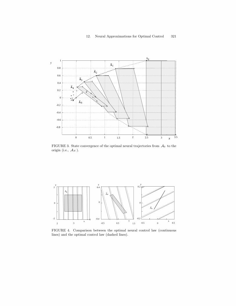
12. Neural Approximations for Optimal Control 321
o2
3
**
**
*
*
*
*
*
* +
+
+
+
+++
A~
A~
A~
A~
A~
4
9
A0*
x
x
x
x o
o
o
o
o
3.532.51.510.50
-0.8
-0.6
-0.4
-0.2
0 o
o
o
x
+
2
1
x
x
0.2
0.4
0.6
0.8
1y
x
o
FIGURE 3. State convergence of the optimal neural trajectories from A0 to theorigin (i.e., AN ).
-2
2 3
4x
0
-0.4
yy
-0.5 0.5 1.5x
0
-0.2
-0.5 0 0.5x
y
A~9
A~4
A0
2
0
0.20.4
FIGURE 4. Comparison between the optimal neural control law (continuouslines) and the optimal control law (dashed lines).

322 Riccardo Zoppoli, Thomas Parisini
e
uT
F
d
_
u 1
2
_
ϑ
y
x
FIGURE 5. The space robot.
Example 2.Consider the space robot presented in Fig. 5, which, for the sake of sim-plicity, is assumed to move in the plane.
The robot position with respect to the coordinate system is described bythe Cartesian coordinates x, y and by the angle ϑ that its axis of symmetry(oriented in the direction of the vector e of unit length) forms with thex axis. Two couples of thrusters, aligned with the axis of symmetry, aremounted on the robot sides. Their thrusts, u1 and u2 , can be modulatedso as to obtain the desired intensity of the force F and the desired torqueT by which to control the robot motion. We assume the mass m and themoment of inertia J to remain constant during the maneuver described inthe following. Then we can write
F = (u1 + u2) e = mdv
dt(24)
T = (u1 − u2) d = Jdω
dt(25)

12. Neural Approximations for Optimal Control 323
8
6
4
2
4 5
3
2
6 7
0
B
00 2 4 6 8
8
9,10
A
B’
A’
10 12x
1
0 5, ,9
43
1
2
¥
FIGURE 6. Positions of the space robot during its maneuver.
where d is the distance between the thrusters and the axis of symmetry,v is the robot velocity, and ω is the angular robot velocity. Let x1 = x ,x2 = x , x3 = y , x4 = y , x5 = ϑ , x6 = ϑ , and x
= col (xi, i = 1, . . . , 6) .
Then, from (24) and (25), we derive the nonlinear differential dynamicsystem
x1 = x2
x2 =1m
(u1 + u2) cos x5
x3 = x4
x4 =1m
(u1 + u2) sin x5
x5 = x6
x6 =d
J(u1 − u2)
(26)
under the constraints|u1| ≤ U , |u2| ≤ U (27)
where U is the maximum thrust value allowed.The space robot is requested to start from any given point of the segment
AB shown in Fig. 6 (the parking edge of a space platform) and to reachan object moving along the segment A′B′ in an unpredictable way.
The dashed line shows the path of the object. When the robot is on thesegment A′B′ , it must stop with the angle ϑ = 0 . Then, the initial andfinal sets are given by
A0 =x ∈ R6 : x1 = 0, x2 = 0, 1 ≤ x3 ≤ 5, x4 = 0, x5 = 0, x6 = 0

324 Riccardo Zoppoli, Thomas Parisini
and
AN =x ∈ R6 : x1 = 10, x2 = 0, 1 ≤ x3 ≤ 5, x4 = 0, x5 = 0, x6 = 0
,
respectively. The maneuver has to be completed at a given time tf , andN = 10 control stages are allowed. The fuel consumption has to be min-imized, and the robot trajectory has to terminate ”sufficiently near” thetarget vector x∗
N . In accordance with these requirements, the cost functioncan be expressed as
J =N−1∑i=0
[c(ui1) + c(ui2) + ‖x∗
N − xi‖2V
]+ ‖x∗
N − xN‖2VN
where xi= x(i∆t) , ui
= u(i∆t) , and ∆t = tf/N (for the sake of brevity,
we do not write the discretized version of the differential system (26), as it issimply given by a first-order Euler’s approximation for the system). More-over, V = diag [1, 0.1, 40, 0.1, 40, 0.1] , VN = diag [40, 40, 40, 40, 40, 40] .The cost of the fuel consumption is taken into account by the functionsc(uij) = k
[1β ln(2 + eβuij + e−βuij ) − 1
β ln(4)], (j = 1, 2) , which approx-
imate (for large enough values of the parameter β ) the nondifferentiablecosts k |uij | (it is realistic to assume the fuel consumption to be propor-tional to the thrust); for the present example, we took β = 50 , k = 0.01 .We also chose c1 = 10−5, c2 = 104, η = 0.9 . The matrices V, VN andthe constant k were chosen such as to obtain a reasonable compromisebetween the ”attractiveness” of the vectors to be tracked and the fuel con-sumption. Note also that the sigmoidal functions generating the controlvariables ui1, ui2 are bounded by unit values. Then, multiplying thesefunctions by U enables us to remove constraints (27). The control func-tions γ (xi, x
∗N , wi) were implemented by means of neural networks with
12 input variables and one hidden layer of 80 units.The positions of the space robot during its maneuver are shown in Fig.
6. The effect of the feedforward action is clearly revealed by the variationoccurring in the robot trajectory when the robot perceives the ”right-aboutturn” of the object to be reached.
7 Statements of the infinite-horizon optimalcontrol problem and of its receding-horizonapproximation
Let us consider again the discrete-time dynamic system (1) that we nowassume to be time-invariant
xt+1 = f(xt, ut), t = 0, 1, . . . (28)
We shall use indexes t for the IH problems, whereas we shall go on usingindexes i for the FH ones. Constraints on state and control vectors areexplicitly taken into account, that is, we assume xt ∈ X ⊂ Rn and

12. Neural Approximations for Optimal Control 325
ut ∈ U ⊂ Rm . In general, denote by Z the class of compact sets A ⊂ Rq
containing the origin as an internal point. This means that A ∈ Z ⇔ ∃λ ∈R, λ > 0 such that N(λ) ⊂ A , where N(λ)
= x ∈ Rq : ‖x‖ ≤ λ is the
closed ball with center 0 and radius λ. Then, assume that X,U ∈ Z . Thecost function is given by
JIH(xt, ut∞) =+∞∑i=t
h(xi, ui) , t ≥ 0 (29)
In (29) and in the following, we define utτ= col (ut, . . . , uτ ) for both finite
and infinite values of the integer τ . Assume that f(0, 0) = 0 and h(0, 0) =0 . Comparing cost (2) with cost (29), we notice that in (29) the cost termsare time-invariant functions and that the cost terms ρi ( ‖x∗
N − xi‖ ) losetheir meanings and then vanish. Now we can state the followingProblem 3. At every time instant t ≥ 0 , find the IH optimal feedbackcontrol law uIH
t = γIH
(xt) ∈ U that minimizes cost (29) for any statext ∈ X .
As is well-known, unless the dynamic system (28) is linear and cost
(29) is quadratic, deriving the optimal feedback law γIH
is a very hard,almost infeasible task. Then, let us now consider an RH approximation forProblem 3. To this end, we need to define the following FH cost function
JFH [xt, ut,t+N−1, N, hF (·)] =t+N−1∑
i=t
h(xi, ui) + hF (xt+N ) , t ≥ 0 (30)
where hF (·) ∈ C1 [Rn,R+] , with hF (0) = 0 , is a suitable terminal costfunction, and N is a positive integer denoting the length of the controlhorizon. Then we can state the followingProblem 4. At every time instant t ≥ 0 , find the RH optimal controllaw uRH
t = γRH
(xt) ∈ U, where uRHt is the first vector of the control
sequence uFHt , . . . , uFH
t+N−1 (i.e., uRHt
= uFH
t ), that minimizes cost (30)for the state xt ∈ X .
As to Problem 4, we remark that stabilizing properties of the RH reg-
ulators were established in [KP77],[KP78],[KBK83], under LQ assump-tions. Extensions to nonlinear systems were derived by Keerthi and Gilbert[KG88] for discrete-time systems and, more recently, by Mayne and Michal-ska [MM90],[MM93] for continuous-time systems. In [MM90], the RH op-timal control problem was solved under the constraint xt+N = 0 . Sucha constraint was relaxed in [MM93] by requiring that the regulator drivethe system to enter a certain neighborhood W of the origin. Once theboundary of W has been reached, a linear regulator, designed to stabilizethe nonlinear system inside W , takes over and steers the state to the ori-gin. It is worth noting that, in both approaches, the regulator computesits control actions on line; this can be accepted only if the process is slowenough, as compared with the computation speed of the regulator itself.
As can be deduced from the statement of Problem 4, we shall derivethe RH stabilizing optimal regulator without imposing either the “exact”

326 Riccardo Zoppoli, Thomas Parisini
constraint xt+N = 0 or the condition of reaching the neighborhood W ofthe origin. The stabilizing property of the RH regulator depends on properchoices of the control horizon N and of the final cost hF (·) that penalizesthe fact that the system state is not steered to the origin at time t + N .
The statement of Problem 4 does not impose any particular way of com-puting the control vector uRH
t as a function of xt . Actually, we have twopossibilities.
1) On-line computation. When the state xt is reached at time t,cost (30) must be minimized at this instant (clearly, no other statebelonging to X is of interest for such minimization). Problem 2 isthen an open-loop optimal control problem and may be regarded asa nonlinear programming one. This problem can be solved on line byconsidering the vectors ut, . . . , ut+N−1, xt+1, . . . , xt+N as indepen-dent variables. The main advantage of this approach is that manywell-established nonlinear programming techniques are available tosolve Problem 2. On the other hand, the approach involves a hugecomputational load for the regulator. If the dynamics of the con-trolled plant is not sufficiently slow, as compared with the speed ofthe regulator’s computing system, a practical application of the RHcontrol mechanism turns out to be infeasible (see [YP93], where amaximum time interval Tc was assigned to the control system to gen-erate the control vector).
2) Off-line computation. By following this approach, the regulatormust be able to generate instantaneously uRH
t for any state xt ∈ Xthat may be reached at stage t. In practice, this implies that the con-trol law γ
RH(xt) has to be computed “a priori” (i.e., off line) and
stored in the regulator’s memory. Clearly, the off-line computationhas advantages and disadvantages that are opposite to the ones ofthe on-line approach. No on-line computational effort is requestedfrom the regulator, but an excessive amount of computer memorymay be required to store the closed-loop control law. Moreover, anN -stage functional optimization problem has to be solved instead of anonlinear programming one. As is well-known, such a functional op-timization problem can be solved analytically only in very few cases,typically under LQ assumptions. As we are looking for feedbackoptimal control laws, dynamic programming seems to be the mostefficient tool. This implies that the control function γ
RH(xt) has to
be computed when the backward phase of the dynamic programmingprocedure, starting from the final stage t + N − 1 , has come backto the initial stage t. Unfortunately, as stated in the first sectionsof the paper, dynamic programming exhibits computational draw-backs that, in general, are very difficult to overcome. In Section 9,we shall return to the off-line solution of Problem 2 and present aneural approximation method to solve this problem.
Here we want to remark that the works by Keerthy and Gilbert and byMayne and Michalska aim to determine the RH optimal control law online, whereas we are more interested in an off-line computational approach.For now, we do not address these computational aspects and, in the nextsection, we present a stabilizing control law to solve Problem 4.

12. Neural Approximations for Optimal Control 327
8 Stabilizing properties of the receding–horizonregulator
As stated in Section 7, we are looking for an RH feedback regulator thatsolves Problem 4, while stabilizing the origin as an equilibrium point of theclosed-loop controlled plant. As previously specified, we relax the exactterminal constraint xt+N = 0 , without imposing the condition of reachinga certain neighborhood W of the origin. Toward this end, the followingassumptions are introduced:
(i) The linear system xt+1 = Axt + But , obtained via the linearizationof system (28) in a neighborhood of the origin, i.e.
A=
∂f
∂xt
∣∣∣∣x
t=0, u
t=0
and B=
∂f
∂ut
∣∣∣∣x
t=0, u
t=0
,
is stabilizable.
(ii) The transition cost function h(x, u) depends on both x and u , andthere exists a strictly increasing function r(·) ∈ C[R+,R+] , withr(0) = 0 , such that h(x, u) ≥ r(‖(x, u)‖), ∀x ∈ X, ∀u ∈ U , where
(x, u)= col (x, u) .
(iii) hF (·) ∈ H(a, P ) , where H(a, P )= hF (·) : hF (x) = a xT Px , for
some a ∈ R , a > 0 , and for some positive-definite symmetric matrixP ∈ Rn×n .
(iv) There exists a compact set X0 ⊂ X, X0 ∈ Z , with the propertythat, for every neighborhood N(λ) ⊂ X0 of the origin of the statespace, there exists a control horizon M ≥ 1 such that there exists asequence of admissible control vectors ui ∈ U, i = t, . . . , t + M − 1that yield an admissible state trajectory xi ∈ X, i = t, t+1, . . . , t+Mending in N(λ) (i.e., xt+M ∈ N(λ) ) for any initial state xt ∈ X0 .
(v) The optimal FH feedback control functions γFH
(xi, i), i = t, . . . , t +N − 1 , which minimize cost (30), are continuous with respect to xi ,for any xt ∈ X and for any finite integer N ≥ 1 .
Assumption (i) is related to the possibility of stabilizing the origin asan equilibrium point of the closed-loop system by using a suitable linearregulator in a neighborhood of the origin itself. In the proof of the followingProposition 4, this assumption is exploited in order to build the regionof attraction for the origin when the RH regulator γ
RH(xt) is applied,
and to provide useful information on the form of the FH cost function(30) that guarantees the stability properties of the control scheme [PZ95].Assumption (i) is the discrete-time version of the one made in [MM93].
Assumption (iii) plays a key role in the development of the stabilityresults concerning the RH regulator, and is essentially related to the relax-ation of the terminal state constraint xt+N = 0 . This is quite consistentwith intuition, as, in practice, the constraint xt+N = 0 is replaced with

328 Riccardo Zoppoli, Thomas Parisini
the final cost hF (·) that penalizes the fact that the system state is notdriven to the origin at time t + N .
Assumption (iv) substantially concerns the controllability of the nonlin-ear system (1). In a sense, it is very similar to the Property C defined in[KG88]. However, assumption (iv) seems to be weaker than this property,which requires the existence of an admissible control sequence that forcesthe system state to reach the origin after a finite number of stages, startingfrom any initial state belonging to Rn .
Let us now denote by JIH(xt) =
+∞∑i=t
h(xIHi , uIH
i ) the cost associated
with the IH optimal trajectory starting from xt (i.e., xIHt = xt ). In an
analogous way, let us denote by JRH [xt, N, hF (·)] =
+∞∑i=t
h(xRHi , uRH
i ) the
cost associated with the RH trajectory starting from xt (i.e., xRHt = xt )
and with the solution of the FH control problem characterized by a controlhorizon N and a terminal cost function hF (·) . Finally, let us denote by
JFH [xt, N, hF (·)]
= JFH [xt, u
t,t+N−1, N, hF (·)]
=t+N−1∑
i=t
h(xFHi , uFH
i ) + hF (xFHt+N )
the cost corresponding to the optimal N -stage trajectory starting from xt .Then, we present the following proposition, which is proved in [PZ95]:
Proposition 4 If assumptions (i) to (v) are verified, there exist a finiteinteger N ≥ M , a positive scalar a and a positive-definite symmetricmatrix P ∈ Rn×n such that, for every terminal cost function hF (·) ∈H(a, P ) , with a ∈ R, a ≥ a , the following properties hold:1) The RH control law stabilizes asymptotically the origin, which is anequilibrium point of the resulting closed-loop system.2) There exists a positive scalar β such that, for any N ≥ N , the set
W[N,hF (·)] ∈ Z , W[N,hF (·)] = x ∈ X : J
FH [x,N, hF (·)] ≤ β , is aninvariant subset of X0 and a domain of attraction for the origin, i.e., forany xt ∈ W[N,hF (·)] , the state trajectory generated by the RH regulatorremains entirely contained in W[N,hF (·)] and converges to the origin.3) For any N ≥ N + 1 , we have
JRH [xt, N, hF (·)] ≤ J
FH [xt, N, hF (·)], ∀xt ∈ W[N,hF (·)] (31)
4) ∀δ ∈ R, δ > 0, there exists an N ≥ N + 1 such that
JRH [xt, N, hF (·)] ≤ J
IH(xt) + δ, ∀xt ∈ W[N,hF (·)] (32)
Proposition 4 asserts that there exist values of a certain number of pa-
rameters, namely, N , P , and a, that ensure us the stabilizing property of

12. Neural Approximations for Optimal Control 329
the RH control law and some nice performances of this regulator, as com-pared with those of the IH one (see (31) and (32)). As nothing is said as tohow such parameters can be found, one is authorized to believe that theycan but be derived by means of some heuristic trial–and–error procedureto test if stability has indeed been achieved. However, some preliminaryresults, based on the rather constructive proof of Proposition 4, as reportedin [PZ95], lead us to believe that appropriate values of N , P , and a canbe computed, at least in principle, by stating and solving some suitableconstrained nonlinear programming problems. We use the words “at leastin principle” because the efficiencies of the related descent algorithms havestill to be verified.
In deriving (both on line and off line) the RH control law uRHt =
γRH
(xt) , computational errors may affect the vector uRHt and possibly
lead to a closed-loop instability of the origin; therefore, we need to establishthe robustness properties of such a control law. This is done by means ofthe following proposition, which characterizes the stabilizing properties ofthe RH regulator when suboptimal control vectors uRH
i ∈ U, i ≥ t are usedin the RH control mechanism, instead of the optimal ones uRH
i solvingProblem 4. Let us denote by xRH
i , i > t , the state vector belonging to thesuboptimal RH trajectory starting from xt .
Proposition 5 If assumptions (i) to (v) are verified, there exist a finiteinteger N , a positive scalar a and a positive-definite symmetric matrixP ∈ Rn×n such that, for any terminal cost function hF (·) ∈ H(a, P ) andfor any N ≥ N , the following properties hold:1) There exist suitable scalars δi ∈ R, δi > 0 such that, if
∥∥∥uRHi − uRH
i
∥∥∥ ≤ δi, i ≥ t,
thenxRH
i ∈ W[N,hF (·)], ∀ i > t, ∀xt ∈ W[N,hF (·)] (33)
2) For any compact set Wd ⊂ Rn, Wd ∈ Z , there exist a finite integerT ≥ t and suitable scalars δi ∈ R, δi > 0 such that, if
∥∥∥uRHi − uRH
i
∥∥∥ ≤ δi, i ≥ t ,
thenxRH
i ∈ Wd , ∀ i ≥ T , ∀xt ∈ W[N,hF (·)] (34)
The proof of Proposition 5 is a direct consequence of the regularity as-sumptions on the state equation (this proof is given in [PZ95]; see also[CPRZ94] for some preliminary results). Proposition 5 has the followingmeaning: the RH regulator can drive the state into every desired neigh-borhood Wd of the origin in a finite time, provided that the errors onthe control vectors are suitably bounded. Moreover, the state will remaincontained in the above neighborhood at any future time instant. Clearly, ifthe RH regulator (generating the above–specified suboptimal control vec-tors) is requested to stabilize the origin asymptotically, the hybrid control

330 Riccardo Zoppoli, Thomas Parisini
mechanism described in [MM93] may be implemented. This involves de-signing an LQ optimal regulator that stabilizes the nonlinear system insidea proper neighborhood W of the origin. Then, if the errors affecting thecontrol vectors generated by the RH regulator are sufficiently small, thisregulator is able to drive the system state inside W (of course, the condi-tion Wd ⊆ W must be satisfied). When the boundary of W is reached,the RH regulator switches to the LQ regulator. It also follows that sucha hybrid control mechanism makes W[N,hF (·)] not only an invariant setbut also a domain of attraction for the origin.
9 The neural approximation for thereceding–horizon regulator
As stated in Section 7, we are mainly interested in computing the RHcontrol law uRH
t = γRH
(xt) off line. This requires that the regulatorgenerate the control vector uRH
t instantaneously, as soon as any statebelonging to the admissible set X is reached. Then, we need to derive (“apriori”) an FH closed-loop optimal control law uFH
i = γFH
(xi, i), t ≥0, i = t, . . . , t + N − 1 , that minimizes cost (30) for any xt ∈ X . Becauseof the time-invariance of the dynamic system (28) and of the cost function(30), we refer to an FH optimal control problem, starting from the statext ∈ X at a generic stage t ≥ 0 . Then, instead of uFH
i = γFH
(xi, i) , weconsider the control functions
uFHi = γ
FH(xi, i − t) , t ≥ 0 , i = t, . . . , t + N − 1 (35)
and state the followingProblem 5. Find the FH optimal feedback control law
uFH
i = γFH
(xi, i − t) ∈ U, t ≥ 0, i = t, . . . , t + N − 1
that minimizes cost (30) for any xt ∈ X .
Once the solution of Problem 5 has been found, we can write
uRHt = γ
RH(xt)
= γ
FH(xt, 0) , ∀xt ∈ X, t ≥ 0 (36)
Dynamic programming seems, at least in principle, the most effective com-putational tool for solving Problem 5. However, this algorithm exhibitsthe well-known computational drawbacks previously pointed out for theFH optimal control problem, namely, the necessity for discretizing (at eachcontrol stage) the set X into a fine enough mesh of grid points, and, con-sequently, the possibility of incurring the curse of dimensionality, even fora small number of state components.
Unlike the requirements related to the N -stage optimal control problemdescribed in the first sections of the paper, it is important to remark thatwe are now interested in determining only the first control function ofthe control law that solves Problem 5, that is, γ
FH(xt, 0) . On the other

12. Neural Approximations for Optimal Control 331
hand, we can compute (off line) any number of open-loop optimal controlsequences uFH
t , . . . , uFHt+N−1 (see Problem 4) for different vectors xt ∈ X .
Therefore, we propose to approximate the function γFH
(xt, 0) by meansof a function γ
FH(xt, w) , to which we assign a given structure. w is a
vector of parameters to be optimized. More specifically, we have to find avector w that minimizes the approximation error
E(w)=∫
X
∥∥∥γFH
(xt, 0) − γFH
(xt, w)∥∥∥2
dxt (37)
Clearly, instead of introducing approximating functions, it would be possi-ble to subdivide the admissible set X into a regular mesh of points, as isusually done at each stage of dynamic programming, and to associate withany point xt ∈ X the control vector uFH
t corresponding to the nearestpoint of the grid. Under the assumption that the function γ
FH(xt, 0) is
continuous in X, it is evident that the mesh should be fine enough to satisfythe conditions required in Proposition 5, i.e.,
∥∥∥uFHi − uFH
i
∥∥∥ ≤ δi, i ≥ t ,
where uFHi are the “true” stabilizing optimal controls (known only for the
grid points), and uFHi are the approximate ones. It is however clear that
the use of such a mesh would lead us again to the unwanted phenomenonof the curse of dimensionality.
For the same reasons as explained in Sections 3 and 4, we choose againa feedforward neural network to implement the approximating functionγ
FH(xt, w) . With respect to Problem 2, it is worth noting that now i)
only one network is needed, and ii) the approximation criterion is differ-ent, in that we have to minimize the approximation error (37), insteadof minimizing the expected process cost. In the following, we refer tothe neural mapping (6),(7), taking into account the fact that the super-script i is useless. The weight and bias coefficients wpq (s) and w0q (s)are the components of the vector w appearing in the approximating func-tion γ
FH(xt, w) ; the variables yq(0) are the components of xt , and the
variables yq(L) are the components of ut . To sum up, once the optimalweight vector w has been derived (off line), the RH neural approximatecontrol law takes on the form
uRHt = γ
RH(xt, w
)= γ
FH(xt, w
) , ∀xt ∈ X , t ≥ 0 (38)
As to the approximating properties of the RH neural regulator, resultssimilar to the ones established in Propositions 2 and 3 can be obtained.Proposition 2 plays an important role also for the stabilizing properties ofthe RH regulator. Then, we repeat it here in a suitably modified version.Proposition1′ Assume that, in the solution of Problem 5, the first con-trol function γ
RH(xt) = γ
FH(xt, 0) of the sequence γ
FH(xi, i − t), i =
t, . . . , t + N − 1 is unique and that it is a C[X,Rm] function. Then, forevery ε ∈ R, ε > 0 , there exist an integer ν and a weight vector w (i.e., aneural RH control law γ(ν)
RH(xt, w) ) such that
∥∥∥γRH
(xt) − γ(ν)
RH(xt, w)
∥∥∥ < ε , ∀xt ∈ X (39)

332 Riccardo Zoppoli, Thomas Parisini
Proposition 1′ enables us to state immediately the following
Corollary [PZ95]. If assumptions (i) to (v) are verified, there exists an RHneural regulator uRH
t = γ(ν)
RH(xt, w), t ≥ 0 , for which the two properties of
Proposition 5 hold true. The control vectors uRHt are constrained to take
on their values from the admissible set U= u : u+∆u ∈ U, ∆u ∈ N(ε) ,
where ε is such that ε ≤ δi, i ≥ t (see the scalars in Proposition 5) andU ∈ Z .
The corollary allows us to apply the results of Proposition 5, thus ob-taining an RH regulator able to drive the system state into any desiredneighborhood Wd of the origin in a finite time. Moreover, with referenceto what has been stated at the end of Section 8, a neural regulator, capableof switching to an LQ stabilizing regulator when a proper neighborhoodW of the origin is reached, makes the region W[N,hF (·)] a domain ofattraction for the origin.
It should be noted that Proposition 1’ and the corollary constitute onlya first step towards the design of a stabilizing neural regulator. In fact,nothing is said as to how the sequence of scalars δi, i ≥ t (hence ε) as wellas the number ν of required neural units can be derived (as we did in com-menting on the computation of the parameters appearing in Proposition 4,we exclude trial–and–error procedures). The determination of the scalarε (see the corollary) is clearly a hard constrained nonlinear optimizationproblem. Hopefully, some algorithm to solve it may be found. To this end,research is currently being conducted.
As to the integer ν, its derivation is an open problem of neural approxi-mation theory, at least if one remains in the class of feedforward neural net-works. If other approximators are addressed, something more can be said.Consider, for example, an approximator given by a nonlinear combina-tion of Gaussian radial basis functions of the form gk(x) = e−‖x−x(k)‖2
/σ2,
where x(k) are fixed centers placed in the nodes of a regular mesh. Sucha mesh is obtained by subdividing the n sides of the smallest hypercubecontaining X into D − 1 segments of length ∆ (a suitable “extension”γ
RH(xt) of γ
RH(xt) outside X must be defined). The number of nodes of
the mesh is then Dn and the components of the approximating functionare given by
γRHj(xt, wj) =Dn∑k=1
wkj gk(xt), j = 1, . . . ,m,
where wj= col (wk
j , k = 1, . . . , Dn) . If the Fourier transform ΓRHj(ω)
of the j–th component of γRH
(xt) is absolutely integrable on Rn , forj = 1, . . . , m , it can be shown [SS92] that
‖ γRH
(xt) − γ(ν)
RH(xt, w) ‖ ≤ ψ , ∀xt ∈ X (40)
where ψ can be made arbitrarily small by suitably choosing the numberD of nodes on the mesh side (or, equivalently, the mesh size ∆) and thevariance σ2. The important result given in [SS92] lies in the fact that such

12. Neural Approximations for Optimal Control 333
parameters can be determined quantitatively on the basis of the smooth-ness characteristics of the function γ
RH(xt) . Such characteristics are
specified by the “significant” frequency ranges of the Fourier transformsΓ
RHj , j = 1, . . . , m and by L1 bounds to these transforms. Note that,as the desired value of ψ decreases, or as the degree of smoothness of thefunction γ
RH(xt) decreases, the variance σ2 and the mesh size ∆ must
suitably decrease (for more details, see [SS92] again). Then, the above re-sults enable one to specify the number ν = mDn of parameters requiredto achieve a given error tolerance. This number reveals that we pay for thepossibility of computing an explicit uniform bound to the approximationerror with the feared danger of incurring the curse of dimensionality.
Coming back to the feedforward neural approximators, it can be expectedthat, given a bound to the approximation error (see (39)), a computationaltechnique will be found to determine the number ν, on the basis of thesmoothness characteristics, also for functions to be approximated that be-long to the difference set between Barron’s class of functions and Sobolevspaces (as said in Section 4, in this difference set, feedforward neural ap-proximators should behave better than linear ones). Waiting for such acomputational technique to be derived, and reassured by the fact that alarge quantity of simulation results lead us to believe that a heuristic (i.e.,experimental) determination of the integer ν is, all things considered, rathereasy, we shall go on with our treatment, still considering feedforward neuralnetworks as our basic approximators. In the next section, we shall presenta method for deriving the weights of this type of networks, and concludeby reporting some simulation results.
10 A gradient algorithm for deriving the RHneural regulator and simulation results
To minimize the approximation error (37), we use again a gradient algo-rithm (see (13)), that is,
w (k + 1) = w (k) − α∇w E [ w (k) ] , k = 0, 1, . . . (41)
Define now the function
D(w, xt)=∥∥∥γ
FH(xt, 0) − γ
FH(xt, w)
∥∥∥2
=∥∥∥γ
RH(xt) − γ
RH(xt, w)
∥∥∥2
,
and note that we are able to evaluate γFH
(xt, 0) only pointwise, that is,by solving Problem 4 for specific values of xt . It follows that we are unableto compute the gradient ∇w E [w(k)] in explicit form. Then, we interpretE (w) as the expected value of the function D(w, xt) by considering xtas a random vector uniformly distributed on X. This leads to use again astochastic approximation approach and to compute the “realization”
∇w D[w, xt(k)],
instead of the gradient appearing in (41).

334 Riccardo Zoppoli, Thomas Parisini
We generate the sequence xt(k), k = 0, 1, . . . randomly, taking intoaccount the fact that xt is considered to be uniformly distributed on X.Then, the updating algorithm becomes
w (k + 1) = w (k) − α(k)∇w D [ w(k), xt(k) ] , k = 0, 1, . . . (42)
To derive the components of
∇wD [w(k), xt(k)] , i.e., the partial derivatives∂D[w(k), xt(k)]
∂wpq(s),
the backpropagation updating rule can be applied again. In the following,we report such a procedure, taking into account the fact that only oneneural network has now to be trained. To simplify the notations, we dropthe index k and define
δq(s)=
∂D [w, xt]∂zq(s)
, s = 1, . . . , L; q = 1, . . . , ns (43)
Then, it is easy to show that
∂D [w, xt]∂wpq(s)
= δq(s)yp(s − 1) (44)
where δq (s) can be computed recursively by means of the equations
δq(s) = g′ [zq(s)]ns+1∑h=1
δh(s + 1)wqh(s + 1) , s = 1, . . . , L − 1 (45a)
δq(L) = g′ [zq(L)]∂D
∂yq(L)(45b)
It can be seen that the algorithm consists of the following two “passes”:Forward pass. The initial state xt(k) is randomly generated from X .Then, the open-loop solution of the FH Problem 4 is computed and thefirst control uFH
t = γFH
[xt(k), 0] is stored in the memory to determine∂D
∂yq(L)(see (45b)). All the variables required by (44) and (45) are stored
in the memory.Backward pass. The variables δq(s) are computed via (45). Then thegradient ∇wD [w(k), xt(k)] is determined by using (44) and the new weightvector w(k + 1) is generated by using (42).
As we said in Sections 9 and 10, further research is needed to derivea computational procedure that gives us the correct values of the param-eters required for the design of a stabilizing RH regulator. However, atleast to judge by the following example, determining experimentally suchparameters may turn out to be quite an easy task.Example 3.

12. Neural Approximations for Optimal Control 335
Consider the same robot as in Example 2. The space robot is now requestedto start from any point of a given region and to reach the origin of the statespace, while minimizing the nonquadratic IH cost
JIH =+∞∑i=0
[c(ui1) + c(ui2) + ‖xi‖2
V
]
For the present example, we chose V = diag [1, 80, 5, 10, 1, 0.1] , β = 50 ,k = 0.01 , c1 = 1, c2 = 108, and ρ = 0.9 . No constraint was imposed on thestate vector. Then, A = x ∈ R6 : −2 ≤ x1 ≤ 2,−0.2 ≤ x2 ≤ 0.2,−2 ≤x3 ≤ 2,−0.2 ≤ x4 ≤ 0.2,−π ≤ x5 ≤ π,−1 ≤ x6 ≤ 1 was chosen as atraining set. The FH cost function takes on the form
JFH =t+N−1∑
i=t
[c(ui1) + c(ui2) + ‖xi‖2
V
]+ a ‖xN‖2
where a = 40 and N = 30 . The control function γFH
(xi, w) , i ≥ t ,was implemented by means of a neural network with six input variablesand one hidden layer of 100 units. Usually, the algorithm converged to theoptimal solution w after 2 · 105 to 3 · 105 iterations.
Figures 7 and 8 show the positions of the space robot along trajectoriesgenerated by the neural RH (NRH) optimal control law. Such trajectoriesare almost indistinguishable from the on-line computed ones, after solvingProblem 4 on line (we denote by ORH the corresponding optimal controllaw). In Fig. 7, the initial velocities x2, x4, x6 are all set to zero, whereas,in Fig. 8, even the initial velocities are not set to zero (in Fig. 8a, we setxt2 = xt4 = 0 ,xt6 = 0.5 , and, in Fig. 8b, xt2 = 0.5 ,xt4 = 0.5 ,xt6 = 0.5 ).It is worth noting that the initial velocities were chosen such as to launchthe space robot along trajectories that were “opposite” to the one thatwould result from initial velocities set to zero (compare the trajectories inFig. 8 with the one shown in Fig. 7a). This causes the trajectories toget out of the set A in the first stages. However, the control actions stillappear quite effective, thus showing the nice “generalization” capabilitiesof the neural RH regulator (i.e., the neural network was tuned even in theneighborhood of the training set A ).
11 Conclusions
Neural approximators have been shown to be powerful and simple approx-imators for solving both FH and RH optimal control problems. Boundsfor the approximations have been given; this is particularly important inRH control schemes, which involve stability issues. Deterministic prob-lems have been addressed; however, the neural approximation approachhas proved effective also for the design of control devices for stochasticdynamic systems [PZ94a] and for optimal state estimators [PZ94c] in non-Gaussian contexts (i.e., outside the classical LQG framework).
As a final remark, it is worth noting that neural approximations en-able us to face even so-called “non-classical” optimal control problems, like

336 Riccardo Zoppoli, Thomas Parisini
-2.5 -2 -1.5 -1 -0.5 0 0.5
-0.5 0
0.5
1
1.5
2
-0.5
0
0.5
1
1.5
2
2.5 2.5
-0.5
0
0.5
1
1.5
2
2.5
x
x
(d)
(b)(a)
(c)
y
x-0.5
y
-0.5
0
0.5
1
1.5
2
2.5
y y
x -2.5 -2 -1.5 -1 -0.5 0 0.5
-2.5 -2 -1.5 -1 -0.5 0 0.5
-2.5 -2 -1.5 -1 -0.5 0 0.5
FIGURE 7. Trajectories of the space robot starting from four different initialpositions at zero initial velocity.
team control problems, characterized by the presence of informationally de-centralized organizations in which several decision makers cooperate on theaccomplishment of a common goal. For this class of problems, quite typicalin large-scale engineering applications, neural methods seem to constitute avery promising tool, as distributed computation, which is a peculiar prop-erty of these methods, may turn out to be a necessity and not a choice (see[PZ93] for an application in the communications area).
Acknowledgments: This work was supported by the Italian Ministry for theUniversity and Research.

12. Neural Approximations for Optimal Control 337
-0.5
0
0.5
1
1.5
2
2.5
3
3.5(a)
-3.5 -3 -2.5 -2 -1.5 -1 -0.5 0 0.5x
y
-0.5
0
0.5
1
1.5
2
2.5
3
3.5(b)
-3.5 -3 -2.5 -2 -1.5 -1 -0.5 0 0.5x
y
FIGURE 8. Trajectories of the space robot starting from the same positions asin the first of the previous figures but at two different sets of initial velocities.
12 References[Bar93] A. R. Barron. Universal approximation bounds for superposi-
tions of a sigmoidal function. IEEE Transactions on Informa-tion Theory, 39:930–945, 1993.
[CPRZ94] A. Cattaneo, T. Parisini, R. Raiteri, and R. Zoppoli. Neuralapproximations for receding-horizon controllers. In Proc. Amer-ican Control Conference, Baltimore, 1994.
[Cyb89] G. Cybenko. Approximations by superpositions of a sigmoidalfunction. Math. Control, Signals, Systems, 2:303–314, 1989.
[ES66] B. R. Eisenberg and A. P. Sage. Closed-loop optimization offixed configuration systems. International Journal of Control,3:183–194, 1966.
[Gir94] F. Girosi. Regularization theory, radial basis functions and net-works. In V. Cherkassky, J.H. Friedman, and H. Wechsler, ed-itors, From Statistics to Neural Networks. Theory and Pattern

338 Riccardo Zoppoli, Thomas Parisini
Recognition Applications. Springer-Verlag, Computer and Sys-tems Sciences, 1994.
[HN89] R. Hecht-Nielsen. Theory of the backpropagation neural net-work. In Proc. IJCNN 1989, Washington, D.C., 1989.
[HSW89] K. Hornik, M. Stinchcombe, and H. White. Multilayer feedfor-ward networks are universal approximators. Neural Networks,2:359–366, 1989.
[Jon92] L. K. Jones. A simple lemma on greedy approximation inHilbert space and convergence rates for projection pursuit re-gression and neural network training. Annals of Statistics,20:608–613, 1992.
[JSS+93] S. A. Johnson, J. D. Stedinger, C. A. Shoemaker, Y. Li, andJ. A. Tejada-Guibert. Numerical solution of continuous-statedynamic programs using linear and spline interpolation. Oper-ations Research, 41:484–500, 1993.
[KA68] D.L. Kleinman and M. Athans. The design of suboptimal lineartime-varying systems. IEEE Trans. Automatic Control, AC-13:150–159, 1968.
[KBK83] W. H. Known, A. M. Bruckstein, and T. Kailath. Stabilizingstate-feedback design via the moving horizon method. Interna-tional Journal of Control, 37:631–643, 1983.
[KG88] S. S. Keerthi and E. G. Gilbert. Optimal infinite-horizon feed-back laws for a general class of constrained discrete-time sys-tems: stability and moving-horizon approximations. Journal ofOptimization Theory and Applications, 57:265–293, 1988.
[KP77] W. H. Known and A. E. Pearson. A modified quadratic costproblem and feedback stabilization of a linear system. IEEETrans. Automatic Control, AC-22:838–842, 1977.
[KP78] W. H. Known and A. E. Pearson. On feedback stabilization oftime-varying discrete linear systems. IEEE Trans. AutomaticControl, AC-23:479–481, 1978.
[Lar68] R. E. Larson. State Increment Dynamic Programming. Ameri-can Elsevier Publishing Company, New York, 1968.
[MM90] D. Q. Mayne and H. Michalska. Receding horizon control ofnonlinear systems. IEEE Trans. on Automatic Control, 35:814–824, 1990.
[MM93] H. Michalska and D. Q. Mayne. Robust receding horizon controlof constrained nonlinear systems. IEEE Trans. on AutomaticControl, 38:1623–1633, 1993.
[MT87] P. M. Makila and H. T. Toivonen. Computational methods forparametric LQ problems- A survey. IEEE Trans. AutomaticControl, AC-32:658–671, 1987.

12. Neural Approximations for Optimal Control 339
[NW90] D. H. Nguyen and B. Widrow. Neural networks for self-learningcontrol systems. IEEE Control System Magazine, 10, 1990.
[Pin86] A. Pinkus. N -Widths in Approximation Theory. Springer-Verlag, New York, 1986.
[PT73] B. T. Polyak and Ya. Z. Tsypkin. Pseudogradient adapta-tion and training algorithms. Automation and Remote Control,12:377–397, 1973.
[PZ93] T. Parisini and R. Zoppoli. Team theory and neural networksfor dynamic routing in traffic and communication networks. In-formation and Decision Technologies, 19:1–18, 1993.
[PZ94a] T. Parisini and R. Zoppoli. Neural approximations for mul-tistage optimal control of nonlinear stochastic systems. InProc. American Control Conference. (to appear also in the IEEETrans. on Automatic Control), Baltimore, 1994.
[PZ94b] T. Parisini and R. Zoppoli. Neural networks for feedback feed-forward nonlinear control systems. IEEE Transactions on Neu-ral Networks, 5:436–449, 1994.
[PZ94c] T. Parisini and R. Zoppoli. Neural networks for nonlinear stateestimation. International Journal of Robust and Nonlinear Con-trol, 4:231–248, 1994.
[PZ95] T. Parisini and R. Zoppoli. A receding-horizon regulator fornonlinear systems and a neural approximation. Automatica,31:1443–1451, 1995.
[RM86] D. E. Rumelhart and J. L. McClelland. Parallel DistributedProcessing. MIT Press, Cambridge, MA, 1986.
[Sag68] A. P. Sage. Optimum Systems Control. Prentice-Hall, Engle-wood Cliffs, 1968.
[SS92] R. M. Sanner and J. J. E. Slotine. Gaussian networks for di-rect adaptive control. IEEE Transactions on Neural Networks,3:837–863, 1992.
[Tsy71] Ya. Z. Tsypkin. Adaptation and Learning in Automatic Sys-tems. Academic Press, New York, 1971.
[YP93] T. H. Yang and E. Polak. Moving horizon control of nonlin-ear systems with input saturation, disturbance and plant un-certainty. International Journal of Control, 58:875–903, 1993.
[ZP92] R. Zoppoli and T. Parisini. Learning techniques and neuralnetworks for the solution of N-stage nonlinear nonquadraticoptimal control problems. In A. Isidori and T. J. Tarn, edi-tors, Systems, Models and Feedback: Theory and Applications.Birkhauser, Boston, 1992.

340 Riccardo Zoppoli, Thomas Parisini

Index
accomodation, 116action potential (AP), 97, 98activation
competitive distribution of, 63activation function, 160, 161, 166,
174, 182, 185, 193, 200,233
Adalines, 1adaptation, 261, 266adaptive control, 280adaptive critic, see critic,adaptive,
260, 267adjoint equation, 319algorithm
EM, 47, 52Forward-Backward, 38Viterbi, 34, 36, 37, 41, 42,
50, 52approximation, 231
-error, 333integrated square, 314, 315uniform, 333
error, 331Euler, 324neural, 314–335receding-horizon (RH), 325stochastic, 317, 333
approximation property, 161, 169,187arm
model, 62, 63, 66–71movement, 63movements, 62robotic, 62
ARMA, 281artificial neural networks, 3ARX, 258ASTREX, 294, 296, 303auto-tuner, 252, 272autoassociative neural networks,
213autonomous control, 280autoregulation, 117
back-propagation, 265back-propagation through time, 266back-propagation-through-time, 268
backpropagation, 130, 150, 158,166, 171, 172, 181, 231,234, 280, 282, 284–286,292, 318, 334
fuzzy, 296backpropagation, dynamic, 129, 131,
136, 139, 150BAM, see bidirectional associa-
tive memorybaroreceptor, 90–120
Type I, 111–113Type II, 111–113
baroreceptor reflex, see baroreflexbaroreflex, 90–120barotopical organization, 95basis function
radial, 279–297basis functions
radial (RBF), 316, 332trigonometric, 315, 316
BDN, 119, 120bidirectional associative memory,
280, 282–284, 287–291,296
eigenstructure, 287biologically organized dynamic net-
work, see BDNblood pressure, 89–120Boltzmann Machine, 46, 47Brunovsky canonical form, 183,
188building control, 263
cardiovascular system, 90, 104, 105cart-pole balancing, 260central pattern generation, 55cerebellar model articulation con-
troller, 280, 282, 292cerebral cortex, see cortex, see cor-
texchemical process, 252chemotaxis, 252, 267, 269CMAC, see cerebellar model ar-
ticulation controllerCMM, see Markov model, con-
trolledco-state variable, 265collinearity of data, 215–217, 222

342 Riccardo Zoppoli, Thomas Parisini
conjugate gradient method, 266connectionist system, 279–281continuous stirred-tank reactor, see
CSTRcontrol
adaptive, 281, 283, 286, 292approximate time-optimal, 228autonomous, 297closed loop, 227, 230feedback feedforward, 310habituating, 105–107learning, 279, 281linear, 235, 239linear state, 241linear state-space, 227min–max approach, 312neural, 282, 287, 291, 294,
296neural RH (NRH), 335optimal, see optimal controlparallel, 103–120parametric optimal, 309reconfigurable, 279, 283, 297smooth, 228specific optimal, 309time-optimal, 227, 235, 236,
239, 241approximate, 242
tracking, 163, 168, 170, 184control system
MISO, 103–105SIMO, 104, 111, 113, 115
controller modeling, 252, 258, 268,272
cortex, 61motor, 63motor (MI), 61, 62proprioceptive, 61–86prorioceptive, 62somatosensory, 62somatosensory (SI), 62
cortical columns, 77clusters of, 63, 86
cortical map formationsimulation of, 71–83
creeping random method, 266critic, 8–25
adaptive, 21–25action-dependent, 25
cross-validation, 214, 223CSTR, 118curse of dimensionality, 309, 315,
316, 330, 331, 333
data
missing values, 208, 210, 212–213
outliers, 210, 211–212preprocessing, 208, 211selecting variables from, 213–
215dead time, 252, 256, 264decoupling, 240, 241delay, c.f. dead time, 268delayed reward, 21direct adaptive control, 260direct neuro-control, 252, 258, 272DP, 25–26dynamic neural network, 253dynamic programming, see DP,
31, 34, 55, 260, 267approximate, 310approximate), 309
dynamic programming), 308, 326,330, 331
dynamics, 280–282, 294–296
EBAM, 280, 287eigenstructure decomposition, 282,
284, 287, 289electric arc furnace, 261eligibility trace, 24error dynamics, 163, 166, 167, 184,
185, 193, 196evaluation function, 21–22, 25evolutionary computing, 267evolutionary optimization, 269
fault detection, 284, 292feedforward networks, 127–131, 136,
140, 143, 148, 149, 151,213
multilayer, 208FEM (finite element model), 295FH, see optimal control, finite-
horizonflight control, 261, 263function space
Barron’s, 309, 314, 333Sobolev, 316, 333
fuzzy control, 267
gain scheduling, 283General Regression Neural Net-
work, see GRNNgenetic algorithm, 252, 267, 269Golgi tendon organs, 70, 71gradient algorithm, 265gradient method, 316, 317gradient-based algorithm, 268

12. Neural Approximations for Optimal Control 343
gradient-based optimization, 265,272
GRNN, 228, 231, 233, 234, 242
habituation, 107–109health monitoring, 279, 284heart, 91, 92, 95, 96, 99, 101, 104,
112hidden layer, 165, 166, 171, 172,
174, 185hidden-layer neurons, 160, 193, 196,
198–200HMM, see Markov model, hiddenHodgkin-Huxley neuron models,
93homeostasis, 89Hopfield network, 117hybrid learning, 286
identification model, 128, 136, 139,140, 143, 145
IH, see optimal control, infinite-horizon
incremental learning, 291indirect neuro-control, 252, 253,
265, 270induction motor drive, 228–230,
235industrial production plant, 241input-output, 132, 133, 140, 143,
145, 150Intelligent Arc Furnace, 261intelligent sensors, 207–223inverse model, 256inverse modeling, 256
joint angle, 67, 68, 70, 71
Kalman filter, 266
lateral inhibition, 96lateral inhibitory network, 43Law of Effect, 7, 8, 14learning, 8
competitive, 66Hebbian, 62, 66reinforcement, 7–27supervised, 8
learning automata, 9–11learning control, 280learning system, 9Levenberg-Marquardt algorithm,
266limit cycles, 235, 239linear model, 258linearization, 141, 142
LMS, 14–17, 23
Manhattan distance, 233map
computational, 61, 62, 65, 66,85
feature, 62, 63sensory feature, 62topographic, 61
map formation, 62, 65Markov
chain, 54process, 50, 52
Markov control, 35Markov decision problem, 37Markov decision problem (MDP),
49Markov model
controlled (CMM), 36, 39variable duration hidden (VDHMM),
47Markov model, hidden (HMM),
31Markov models
controlled (CMM), 34–40Markov process, 33, 38, 39, 50
controlled, 32partially observed, 38
Mexican Hat, 62, 65Miltech-NOH, 261MIMO, 234, 236model predictive control, 254model-based control, 254model-based controller, 272model-based neuro-control, 252, 259,
260, 268model-free controller, 272model-free neuro-control, 252, 259,
267models
input-output, 127, 128–150state space, 128, 129, 139, 150
momentum, 266motor neurons
postganglionic, 104, 105vagal, 104, 105
MPC controller, 254, 256, 259Multi-Input/Multi-Output, see MIMOmultilayer Perceptron, 267muscle, 62–86
abductor and adductor, 63,67, 68
agonist and antagonist, 67antagonist, 61flexor and extensor, 63, 67,
68, 79, 83

344 Riccardo Zoppoli, Thomas Parisini
length and tension, 71–75, 77stretch, 62tension, 62
NARMAX, 253NARX, 253Neural Applications Corporation,
261neural control, 279, 281, 282neural network
feed-forward, 34, 56neural network auto-tuner, 252,
257neural network inverse model, 255neural network inverse model-based
control, 252neural network model-based con-
trol, 252, 253neural networks
multilayer feedforward, 309,311
neuron modelHopfield, 117
nip-section, 228, 236, 241, 242non-gradient algorithm, 265, 266non-gradient based optimization,
272non-gradient-based optimization,
251, 267nonlinear optimization, 251, 252nonlinear programming, 307, 309,
310, 313, 316, 326NTS, 91–95, 116nucleus tractus solitarii, see NTS
objective function, 252observability, 129–147
generic, 132–150strong, 132
observability matrix, 133observability, generic, 134, 145–
147observability, strong, 134, 141, 143,
145optimal control
finite-horizon (FH), 307–335infinite-horizon (IH), 308–335linear-quadratic, 308, 325linear-quadratic), 310receding-horizon (RH), 308–
335
parameterized neuro-controller, 251,263, 272
parametric neural network, 254parasympathetic system, 104, 105,
112
partial least squaresneural network (NNPLS), 220–
222partial least squares (PLS), 213,
219partitioned neural networks, 181,
182passivity of neural network, 158,
161, 162, 177, 181strict, 157, 162, 164, 177, 181,
203PCA, see principle component anal-
ysisperceptron, 1, 3peripheral resistance, 99, 104, 105,
112phase plane, 239phoneme, 45, 47, 56PI controller, 269PID controller, 257, 258, 263, 264,
270, 272PLS, see partial least squaresPNC, see paramaterized neuro-controllerpolymerization, 105–107potassium current, 97predictive control, 281principle component analysis (PCA),
209, 212, 219principle component regression (PCR),
213, 215process control, 263process model, 251–253, 255, 257,
258, 260–262, 266, 268,272
process model mismatch, 263process soft sensors, 207, 208, 222proprioception, map formation, 62
Q-learning, 24–26quasi-Newton optimization, 258
radial basis function, see basis func-tion, radial
radial basis function network, 267radial basis function networks, adap-
tive time-delay, 280Radial basis functions, 228random search, 266RBF, see radial basis functionRBF network, 279–297receptor
stretch, 70recurrent network, 253, 267recurrent networks, 127–129, 131redundancy, 283, 291regression matrix, 159, 174, 203

12. Neural Approximations for Optimal Control 345
regulation problem, 308reinforcement learning, 260restrictions, 235, 236reverse engineering, 95, 106, 113RH, see control, receding-horizon,
325ridge function, 3ridge regression, 207, 209, 218, 219,
222robot arm, 62robot arm, control of, 162–164,
168, 171, 172, 174, 181,182, 188
robust backpropagation, 212robust model, 263robust model-based neuro-control,
252, 262robust performance, 263robust stability, 262robustness, 262robustness of controller, 158, 167,
177, 185
scheduling algorithms, 102second-order method, 266self-organization– cortical maps,
62sensitivity analysis, 214, 222servomechanism problem, 307sigmoids, 3simulated annealing, 267singular value decomposition, 290,
291singular value decomposition (SVD),
289skew-symmetry property– robot arm,
163, 164space robot, 322–335space structures, 279, 282, 291,
293, 294, 297speech recognition, 50, 53, 55, 56spindle, see receptor, stretchstability
global, 287, 289structural, 287, 289
state space, 146statistical methods, 207, 212, 213,
222stretch receptor, see receptor, stretchstretch receptors, see barorecep-
torssupervised learning, 253, 265switching, 236, 237sympathetic system, 99, 104, 105,
112system identification, 282, 296
TDL (tapped delay lines), 281time-optimal, see control, time-
optimaltorque, motor, 230, 235, 236, 240tracking error, 163, 164, 168, 169,
171, 173, 181, 186, 187,190, 191
transputers, 232transversal, 134, 135, 146, 152,
153truck-backer-upper, 261
uniformly ultimately bounded (UUB),161, 195
unmyelinated fibers, 112
VDHMM, see Markov model, vari-able duration hidden
vibration suppression, 279, 281,295
Viterbi algorithm, see algorithmViterbi score, 34, 37, 41
web, 227, 228, 235web force, 230web forces, 227, 230Wiener, Norbert, 1
XOR problem, 234
zero-trajectory, 235