Neural Networks - Penn Engineering › ~cis519 › fall2017 › lectures › 11_Neura… · • Neural networks are designed to be massively parallel • The brain is effectively

NeuralNetworks

1Robot Image Credit: Viktoriya Sukhanova © 123RF.com

These slides were assembled by Eric Eaton, with grateful acknowledgement of the many others who made their course materials freely available online. Feel free to reuse or adapt these slides for your own academic purposes, provided that you include proper attribution. Please send comments and corrections to Eric.

NeuralFunction• Brainfunction(thought)occursastheresultofthefiringofneurons

• Neuronsconnecttoeachotherthroughsynapses,whichpropagateactionpotential (electricalimpulses)byreleasingneurotransmitters– Synapsescanbeexcitatory(potential-increasing)orinhibitory(potential-decreasing),andhavevaryingactivationthresholds

– Learningoccursasaresultofthesynapses’ plasticicity:Theyexhibitlong-termchangesinconnectionstrength

• Thereareabout1011neuronsandabout1014synapsesinthehumanbrain!

2BasedonslidebyT.Finin,M.desJardins,LGetoor,R.Par

BiologyofaNeuron

3

BrainStructure• Differentareasofthebrainhavedifferentfunctions

– Someareasseemtohavethesamefunctioninallhumans(e.g.,Broca’s regionformotorspeech);theoveralllayoutisgenerallyconsistent

– Someareasaremoreplastic,andvaryintheirfunction;also,thelower-levelstructureandfunctionvarygreatly

• Wedon’tknowhowdifferentfunctionsare“assigned” oracquired– Partlytheresultofthephysicallayout/connectiontoinputs(sensors)andoutputs(effectors)

– Partlytheresultofexperience(learning)

• Wereally don’tunderstandhowthisneuralstructureleadstowhatweperceiveas“consciousness” or“thought”


The“OneLearningAlgorithm”Hypothesis

5

Auditorycortexlearnstosee

AuditoryCortex

[Roeetal.,1992]

Somatosensorycortexlearnstosee

[Metin &Frost,1989]

SomatosensoryCortex

BasedonslidebyAndrewNg

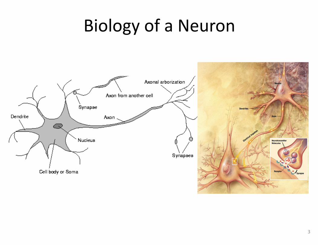
SensorRepresentationsintheBrain

6

Seeingwithyourtongue Humanecholocation(sonar)

Haptic belt:Directionsense Implantinga3rd eye

[BrainPort;Welsh&Blasch,1997;Nageletal.,2005;Constantine-Paton&Law,2009]

SlidebyAndrewNg

Comparisonofcomputingpower

• Computersarewayfasterthanneurons…• Buttherearealotmoreneuronsthanwecanreasonably

modelinmoderndigitalcomputers,andtheyallfireinparallel

• Neuralnetworksaredesignedtobemassivelyparallel• Thebrainiseffectivelyabilliontimesfaster

INFORMATIONCIRCA2012 Computer HumanBrainComputationUnits 10-coreXeon:109 Gates 1011 Neurons

StorageUnits 109 bitsRAM,1012 bitsdisk 1011 neurons,1014 synapses

Cycletime 10-9 sec 10-3 sec

Bandwidth 109 bits/sec 1014 bits/sec

7

NeuralNetworks• Origins:Algorithmsthattrytomimicthebrain.• Verywidelyusedin80sandearly90s;popularitydiminishedinlate90s.

• Recentresurgence:State-of-the-arttechniqueformanyapplications

• Artificialneuralnetworksarenotnearlyascomplexorintricateastheactualbrainstructure

8BasedonslidebyAndrewNg

Neuralnetworks

• Neuralnetworksaremadeupofnodes orunits,connectedbylinks

• Eachlinkhasanassociatedweight andactivationlevel• Eachnodehasaninputfunction (typicallysummingover

weightedinputs),anactivationfunction,andanoutput

Output units

Hidden units

Input unitsLayered feed-forward network


NeuronModel:LogisticUnit

10

Sigmoid(logistic)activationfunction: g(z) =1

1 + e�z

h✓(x) =1

1 + e�✓Tx

h✓(x) = g (✓|x)

x0 = 1x0 = 1

“biasunit”

h✓(x) =1

1 + e�✓Tx

x =

2

664

x0

x1

x2

x3

3

775 ✓ =

2

664

✓0✓1✓2✓3

3

775✓0

✓1

✓2

✓3


X

h✓(x) =1

1 + e�✓Tx

NeuralNetwork

12

Layer3(OutputLayer)

Layer1(InputLayer)

Layer2(HiddenLayer)

x0 = 1biasunits a(2)0

SlidebyAndrewNg

Feed-Forward Process• Inputlayerunitsaresetbysomeexteriorfunction(thinkoftheseassensors),whichcausestheiroutputlinkstobeactivated atthespecifiedlevel

• Workingforwardthroughthenetwork,theinputfunction ofeachunitisappliedtocomputetheinputvalue– Usuallythisisjusttheweightedsumoftheactivationonthelinksfeedingintothisnode

• Theactivationfunction transformsthisinputfunctionintoafinalvalue– Typicallythisisanonlinear function,oftenasigmoidfunctioncorrespondingtothe“threshold” ofthatnode


NeuralNetwork

14

ai(j) = “activation”ofuniti inlayerjΘ(j) = weightmatrixcontrollingfunction

mappingfromlayerj tolayerj +1

Ifnetworkhassj unitsinlayerj andsj+1 unitsinlayerj+1,thenΘ(j) hasdimensionsj+1 × (sj+1) .

⇥(1) 2 R3⇥4 ⇥(2) 2 R1⇥4

SlidebyAndrewNg

h✓(x) =1

1 + e�✓Tx

⇥(1) ⇥(2)

Feed-ForwardSteps:

Vectorization

15

a

(2)1 = g

⇣⇥(1)

10 x0 +⇥(1)11 x1 +⇥(1)

12 x2 +⇥(1)13 x3

⌘= g

⇣z

(2)1

⌘

a

(2)2 = g

⇣⇥(1)

20 x0 +⇥(1)21 x1 +⇥(1)

22 x2 +⇥(1)23 x3

⌘= g

⇣z

(2)2

⌘

a

(2)3 = g

⇣⇥(1)

30 x0 +⇥(1)31 x1 +⇥(1)

32 x2 +⇥(1)33 x3

⌘= g

⇣z

(2)3

⌘

h⇥(x) = g

⇣⇥(2)

10 a(2)0 +⇥(2)

11 a(2)1 +⇥(2)

12 a(2)2 +⇥(2)

13 a(2)3

⌘= g

⇣z

(3)1

⌘

a

(2)1 = g

⇣⇥(1)

10 x0 +⇥(1)11 x1 +⇥(1)

12 x2 +⇥(1)13 x3

⌘= g

⇣z

(2)1

⌘

a

(2)2 = g

⇣⇥(1)

20 x0 +⇥(1)21 x1 +⇥(1)

22 x2 +⇥(1)23 x3

⌘= g

⇣z

(2)2

⌘

a

(2)3 = g

⇣⇥(1)

30 x0 +⇥(1)31 x1 +⇥(1)

32 x2 +⇥(1)33 x3

⌘= g

⇣z

(2)3

⌘

h⇥(x) = g

⇣⇥(2)

10 a(2)0 +⇥(2)

11 a(2)1 +⇥(2)

12 a(2)2 +⇥(2)

13 a(2)3

⌘= g

⇣z

(3)1

⌘

a

(2)1 = g

⇣⇥(1)

10 x0 +⇥(1)11 x1 +⇥(1)

12 x2 +⇥(1)13 x3

⌘= g

⇣z

(2)1

⌘

a

(2)2 = g

⇣⇥(1)

20 x0 +⇥(1)21 x1 +⇥(1)

22 x2 +⇥(1)23 x3

⌘= g

⇣z

(2)2

⌘

a

(2)3 = g

⇣⇥(1)

30 x0 +⇥(1)31 x1 +⇥(1)

32 x2 +⇥(1)33 x3

⌘= g

⇣z

(2)3

⌘

h⇥(x) = g

⇣⇥(2)

10 a(2)0 +⇥(2)

11 a(2)1 +⇥(2)

12 a(2)2 +⇥(2)

13 a(2)3

⌘= g

⇣z

(3)1

⌘

a

(2)1 = g

⇣⇥(1)

10 x0 +⇥(1)11 x1 +⇥(1)

12 x2 +⇥(1)13 x3

⌘= g

⇣z

(2)1

⌘

a

(2)2 = g

⇣⇥(1)

20 x0 +⇥(1)21 x1 +⇥(1)

22 x2 +⇥(1)23 x3

⌘= g

⇣z

(2)2

⌘

a

(2)3 = g

⇣⇥(1)

30 x0 +⇥(1)31 x1 +⇥(1)

32 x2 +⇥(1)33 x3

⌘= g

⇣z

(2)3

⌘

h⇥(x) = g

⇣⇥(2)

10 a(2)0 +⇥(2)

11 a(2)1 +⇥(2)

12 a(2)2 +⇥(2)

13 a(2)3

⌘= g

⇣z

(3)1

⌘


z

(2) = ⇥(1)x

a

(2) = g(z(2))

Add a(2)0 = 1

z

(3) = ⇥(2)a

(2)

h⇥(x) = a

(3) = g(z(3))

z

(2) = ⇥(1)x

a

(2) = g(z(2))

Add a(2)0 = 1

z

(3) = ⇥(2)a

(2)

h⇥(x) = a

(3) = g(z(3))

z

(2) = ⇥(1)x

a

(2) = g(z(2))

Add a(2)0 = 1

z

(3) = ⇥(2)a

(2)

h⇥(x) = a

(3) = g(z(3))⇥(1) ⇥(2)

h✓(x) =1

1 + e�✓Tx

OtherNetworkArchitectures

L denotesthenumberoflayers

containsthenumbersofnodesateachlayer– Notcountingbiasunits– Typically,s0 = d (#inputfeatures)andsL-1=K (#classes)

16

Layer3Layer1 Layer2 Layer4

h✓(x) =1

1 + e�✓Tx

s 2 N+L

s =[3,3,2,1]

MultipleOutputUnits:One-vs-Rest

17

Pedestrian Car Motorcycle Truck

h⇥(x) 2 RK

whenpedestrianwhencarwhenmotorcyclewhentruck

h⇥(x) ⇡

2

664

0001

3

775h⇥(x) ⇡

2

664

0010

3

775h⇥(x) ⇡

2

664

0100

3

775h⇥(x) ⇡

2

664

1000

3

775

Wewant:

SlidebyAndrewNg

MultipleOutputUnits:One-vs-Rest

• Given{(x1,y1), (x2,y2), ..., (xn,yn)}• Mustconvertlabelsto1-of-K representation

– e.g.,whenmotorcycle,whencar,etc.18

h⇥(x) 2 RK

whenpedestrianwhencarwhenmotorcyclewhentruck

h⇥(x) ⇡

2

664

0001

3

775h⇥(x) ⇡

2

664

0010

3

775h⇥(x) ⇡

2

664

0100

3

775h⇥(x) ⇡

2

664

1000

3

775

Wewant:

yi =

2

664

0100

3

775yi =

2

664

0010

3

775


NeuralNetworkClassification

19

Binaryclassificationy =0or1

1outputunit(sL-1= 1)

Multi-classclassification (K classes)

K outputunits(sL-1= K)

y 2 RK

pedestriancarmotorcycletruck

e.g.,,,

Given:{(x1,y1), (x2,y2), ..., (xn,yn)}

contains#nodesateachlayer– s0 = d (#features)

s 2 N+L

SlidebyAndrewNg

UnderstandingRepresentations

20

RepresentingBooleanFunctions

21

Simpleexample:AND

x1 x2 hΘ(x)0 00 11 01 1

g(z) =1

1 + e�z

Logistic/SigmoidFunction

hΘ(x) = g(-30 + 20x1 + 20x2)

-30

+20

+20h✓(x) =

1

1 + e�✓Tx

BasedonslideandexamplebyAndrewNg

x1 x2 hΘ(x)0 0 g(-30) ≈00 1 g(-10) ≈01 0 g(-10) ≈01 1 g(10) ≈1

RepresentingBooleanFunctions

22

-10

+20+20

h✓(x) =1

1 + e�✓Tx

OR-30

+20+20

h✓(x) =1

1 + e�✓Tx

AND

+10

-20h✓(x) =

1

1 + e�✓Tx

NOT+10

-20-20

h✓(x) =1

1 + e�✓Tx

(NOTx1)AND(NOTx2)

CombiningRepresentationstoCreateNon-LinearFunctions

23

-10+20+20

h✓(x) =1

1 + e�✓Tx

OR-30

+20+20

h✓(x) =1

1 + e�✓Tx

AND+10

-20-20

h✓(x) =1

1 + e�✓Tx

(NOTx1)AND(NOTx2)

III

III IV

not(XOR)-10

+20

+20h✓(x) =

1

1 + e�✓Tx

-30+20

+20 inI

+10-20

-20

inIII I or III

BasedonexamplebyAndrewNg

LayeringRepresentations

Eachimageis“unrolled”intoavectorx ofpixelintensities

24

20× 20pixelimagesd =40010classes

x1 ... x20x21 ... x40x41 ... x60

x381 ... x400

...

LayeringRepresentations

25

x1

x2

x3

x4

x5

xd

“0”

“1”

“9”

InputLayer

OutputLayerHiddenLayer

VisualizationofHiddenLayer

26

LeNet 5Demonstration:http://yann.lecun.com/exdb/lenet/

NeuralNetworkLearning

27

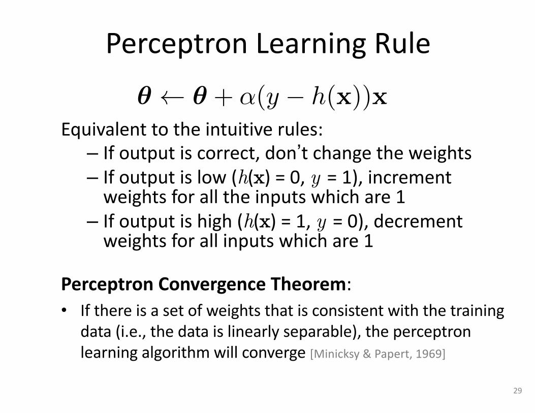
PerceptronLearningRule

Equivalenttotheintuitiverules:– Ifoutputiscorrect,don’tchangetheweights– Ifoutputislow(h(x)=0,y =1),incrementweightsforalltheinputswhichare1

– Ifoutputishigh(h(x)=1,y =0),decrementweightsforallinputswhichare1

PerceptronConvergenceTheorem:• Ifthereisasetofweightsthatisconsistentwiththetraining

data(i.e.,thedataislinearlyseparable),theperceptronlearningalgorithmwillconverge[Minicksy &Papert,1969]

29

✓ ✓ + ↵(y � h(x))x

BatchPerceptron

30

1.) Given training data

�(x

(i), y(i)) n

i=12.) Let ✓ [0, 0, . . . , 0]2.) Repeat:

2.) Let � [0, 0, . . . , 0]3.) for i = 1 . . . n, do4.) if y(i)x(i)

✓ 0 // prediction for i

thinstance is incorrect

5.) � �+ y(i)x(i)

6.) � �/n // compute average update

6.) ✓ ✓ + ↵�8.) Until k�k2 < ✏

• Simplestcase:α=1anddon’tnormalize,yieldsthefixedincrementperceptron

• EachincrementofouterloopiscalledanepochBasedonslidebyAlanFern

LearninginNN:Backpropagation• Similartotheperceptronlearningalgorithm,wecyclethroughourexamples– Iftheoutputofthenetworkiscorrect,nochangesaremade– Ifthereisanerror,weightsareadjustedtoreducetheerror

• Thetrickistoassesstheblamefortheerroranddivideitamongthecontributingweights


J(✓) = � 1

n

nX

i=1

[yi log h✓(xi) + (1� yi) log (1� h✓(xi))] +�

2n

dX

j=1

✓2j

CostFunction

32

LogisticRegression:

NeuralNetwork:

h⇥ 2 RK(h⇥(x))i = ithoutput

J(⇥) =� 1

n

"nX

i=1

KX

k=1

yik log (h⇥(xi))k + (1� yik) log⇣1� (h⇥(xi))k

⌘#

+

�

2n

L�1X

l=1

sl�1X

i=1

slX

j=1

⇣⇥

(l)ji

⌘2


J(⇥) =� 1

n

"nX

i=1

KX

k=1


⌘#

+

�

2n

L�1X

l=1

sl�1X

i=1

slX

j=1

⇣⇥

(l)ji

⌘2


J(⇥) =� 1

n

"nX

i=1

KX

k=1


⌘#

+

�

2n

L�1X

l=1

sl�1X

i=1

slX

j=1

⇣⇥

(l)ji

⌘2 kth class: true,predictednotkth class: true,predicted


OptimizingtheNeuralNetwork

33

Needcodetocompute:••

Solvevia:

J(⇥) =� 1

n

"nX

i=1

KX

k=1

yik log(h⇥(xi))k + (1� yik) log⇣1� (h⇥(xi))k

⌘#

+

�

2n

L�1X

l=1

sl�1X

i=1

slX

j=1

⇣⇥

(l)ji

⌘2

J(Θ) isnotconvex,soGDonaneuralnetyieldsalocaloptimum• But,tendstoworkwellinpractice


ForwardPropagation• Givenonelabeledtraininginstance(x, y):

ForwardPropagation• a(1) = x• z(2) = Θ(1)a(1)

• a(2) = g(z(2)) [adda0(2)]

• z(3) = Θ(2)a(2)

• a(3) = g(z(3)) [adda0(3)]

• z(4) = Θ(3)a(3)

• a(4) = hΘ(x) = g(z(4))

34

a(1)

a(2) a(3) a(4)


Backpropagation Intuition• Eachhiddennodej is“responsible” forsomefractionoftheerrorδj(l) ineachoftheoutputnodestowhichitconnects

• δj(l) isdividedaccordingtothestrengthoftheconnectionbetweenhiddennodeandtheoutputnode

• Then,the“blame”ispropagatedbacktoprovidetheerrorvaluesforthehiddenlayer


�(l)j =

@

@z(l)j

cost(xi)

where cost(xi) = yi log h⇥(xi) + (1� yi) log(1� h⇥(xi))

Backpropagation Intuition

δj(l) = “error”ofnodej inlayerlFormally,

36

�(4)1�(3)1�(2)1

�(2)2 �(3)2




37

�(4)1�(3)1�(2)1

�(2)2 �(3)2


δ(4) = a(4) – y

�(l)j =

@

@z(l)j

cost(xi)




38

�(4)1�(3)1�(2)1

�(2)2 �(3)2

⇥(3)12

δ2(3) = Θ12(3)×δ1(4)


�(l)j =

@

@z(l)j

cost(xi)




39

�(3)1�(2)1

�(2)2 �(3)2

δ2(3) = Θ12(3) ×δ1(4)

δ1(3) = Θ11(3)×δ1(4)

�(4)1


�(l)j =

@

@z(l)j

cost(xi)




40

�(4)1�(3)1�(2)1

�(2)2 �(3)2

⇥(2)12

⇥(2)22

δ2(2) = Θ12(2)×δ1(3) +Θ22

(2)×δ2(3)


�(l)j =

@

@z(l)j

cost(xi)


Backpropagation:GradientComputationLetδj(l) = “error”ofnodej inlayerl

(#layersL =4)

Backpropagation• δ(4) = a(4) – y• δ(3) = (Θ(3))Tδ(4) .* g’(z(3)) • δ(2) = (Θ(2))Tδ(3) .* g’(z(2))• (Noδ(1))

41

g’(z(3)) = a(3) .* (1–a(3))

g’(z(2)) = a(2) .* (1–a(2))

@

@⇥(l)ij

J(⇥) = a(l)j �(l+1)i (ignoringλ;ifλ = 0)

δ(4)δ(3)δ(2)

Element-wiseproduct.*


Backpropagation

42

Note:Canvectorize as�(l)

ij = �(l)ij + a(l)j �(l+1)

i

�(l) = �(l) + �(l+1)a(l)|

�(l)ij = �(l)

ij + a(l)j �(l+1)i

�(l) = �(l) + �(l+1)a(l)|

Given: training set {(x1, y1), . . . , (xn, yn)}Initialize all ⇥(l) randomly (NOT to 0!)Loop // each iteration is called an epoch

Set �(l)ij = 0 8l, i, j

For each training instance (xi, yi):Set a(1) = xi

Compute {a(2), . . . ,a(L)} via forward propagationCompute �(L) = a

(L) � yiCompute errors {�(L�1), . . . , �(2)}Compute gradients �

(l)ij = �

(l)ij + a(l)j �(l+1)

i

Compute avg regularized gradient D(l)ij =

(1n�

(l)ij + �⇥(l)

ij if j 6= 01n�

(l)ij otherwise

Update weights via gradient step ⇥(l)ij = ⇥

(l)ij � ↵D(l)

ijUntil weights converge or max #epochs is reachedD(l) isthematrixofpartialderivativesofJ(Θ)



Set �(l)ij = 0 8l, i, j




(l)ij = �

(l)ij + a(l)j �(l+1)

i


(1n�

(l)ij + �⇥(l)

ij if j 6= 01n�

(l)ij otherwise


(l)ij � ↵D(l)

ijUntil weights converge or max #epochs is reached


Set �(l)ij = 0 8l, i, j




(l)ij = �

(l)ij + a(l)j �(l+1)

i


(1n�

(l)ij + �⇥(l)

ij if j 6= 01n�

(l)ij otherwise


(l)ij � ↵D(l)



Set �(l)ij = 0 8l, i, j




(l)ij = �

(l)ij + a(l)j �(l+1)

i


(1n�

(l)ij + �⇥(l)

ij if j 6= 01n�

(l)ij otherwise


(l)ij � ↵D(l)



Set �(l)ij = 0 8l, i, j




(l)ij = �

(l)ij + a(l)j �(l+1)

i


(1n�

(l)ij + �⇥(l)

ij if j 6= 01n�

(l)ij otherwise


(l)ij � ↵D(l)


(Usedtoaccumulategradient)


Set �(l)ij = 0 8l, i, j




(l)ij = �

(l)ij + a(l)j �(l+1)

i


(1n�

(l)ij + �⇥(l)

ij if j 6= 01n�

(l)ij otherwise


(l)ij � ↵D(l)


TrainingaNeuralNetworkviaGradientDescentwithBackprop

43


Set �(l)ij = 0 8l, i, j




(l)ij = �

(l)ij + a(l)j �(l+1)

i


(1n�

(l)ij + �⇥(l)

ij if j 6= 01n�

(l)ij otherwise


(l)ij � ↵D(l)


(Usedtoaccumulategradient)


Backpropagation

Backprop Issues“Backprop isthecockroachofmachinelearning.It’sugly,andannoying,butyoujustcan’tgetridofit.”

-GeoffHinton

Problems:• blackbox• localminima

44

ImplementationDetails

45

RandomInitialization• Importanttorandomizeinitialweightmatrices• Can’thaveuniforminitialweights,asinlogisticregression

– Otherwise,allupdateswillbeidentical&thenetwon’tlearn

46

�(4)1�(3)1�(2)1

�(2)2 �(3)2

ImplementationDetails• Forconvenience,compressallparametersintoθ

– “unroll”Θ(1), Θ(2),... , Θ(L-1) intoonelongvectorθ• E.g.,ifΘ(1) is10x10,thenthefirst100entriesofθ containthevalueinΘ(1)

– Usethereshape commandtorecovertheoriginalmatrices• E.g.,ifΘ(1) is10x10,then

theta1 = reshape(theta[0:100], (10, 10))

• Eachstep,checktomakesurethatJ(θ) decreases

• Implementagradient-checkingproceduretoensurethatthegradientiscorrect...

47

J(✓i+c)

J(✓i�c)

✓i�c ✓i+c

GradientCheckingIdea: estimategradientnumericallytoverifyimplementation,thenturnoffgradientchecking

49

θi+c = [θ1, θ2, ..., θi –1, θi+c, θi+1, ...]

c ⇡ 1E-4@

@✓iJ(✓) ⇡ J(✓i+c)� J(✓i�c)

2c

J(✓)

ChangeONLYthei th

entryinθ,increasing(ordecreasing)itbyc


GradientChecking

50

✓ 2 Rm ✓ is an “unrolled” version of ⇥

(1),⇥(2), . . .

✓ = [✓1, ✓2, ✓3, . . . , ✓m]

@

@✓1J(✓) ⇡ J([✓1 + c, ✓2, ✓3, . . . , ✓m])� J([✓1 � c, ✓2, ✓3, . . . , ✓m])

2c@

@✓2J(✓) ⇡ J([✓1, ✓2 + c, ✓3, . . . , ✓m])� J([✓1, ✓2 � c, ✓3, . . . , ✓m])

2c.

.

.

@

@✓mJ(✓) ⇡ J([✓1, ✓2, ✓3, . . . , ✓m + c])� J([✓1, ✓2, ✓3, . . . , ✓m � c])

2c

CheckthattheapproximatenumericalgradientmatchestheentriesintheDmatrices

PutinvectorcalledgradApprox


ImplementationSteps• Implementbackprop tocomputeDVec

– DVec istheunrolled{D(1), D(2), ... }matrices

• ImplementnumericalgradientcheckingtocomputegradApprox• MakesureDVec hassimilarvaluestogradApprox• Turnoffgradientchecking.Usingbackprop codeforlearning.

Important:Besuretodisableyourgradientcheckingcodebeforetrainingyourclassifier.• Ifyourunthenumericalgradientcomputationoneveryiteration

ofgradientdescent,yourcodewillbevery slow


PuttingItAllTogether

52

TrainingaNeuralNetworkPickanetworkarchitecture(connectivitypatternbetweennodes)

• #inputunits=#offeaturesindataset• #outputunits=#classes

Reasonabledefault:1hiddenlayer• orif>1hiddenlayer,havesame#hiddenunitsineverylayer(usuallythemorethebetter)


TrainingaNeuralNetwork1. Randomlyinitializeweights2. ImplementforwardpropagationtogethΘ(xi)

foranyinstancexi

3. ImplementcodetocomputecostfunctionJ(Θ)4. Implementbackprop tocomputepartialderivatives

5. Usegradientcheckingtocomparecomputedusingbackpropagation vs.thenumericalgradientestimate.– Then,disablegradientcheckingcode

6. Usegradientdescentwithbackprop tofitthenetwork54BasedonslidebyAndrewNg

Documents

Neural Networks - Penn Engineering › ~cis519 › fall2017 › lectures › 11_Neura… · • Neural networks are designed to be massively parallel • The brain is effectively