Embed Size (px)
Citation preview
Neural Networks for System Modeling • Gábor Horváth, 2005 Budapest University of Technology and Economics
Gábor Horváth
Budapest University of Technology and Economics
Dept. Measurement and Information Systems
Budapest, Hungary
Copyright © Gábor HorváthThe slides are based on the NATO ASI presentation (NIMIA) in Crema Italy, 2002
NEURAL NETWORKS FOR SYSTEM MODELING
Neural Networks for System Modeling • Gábor Horváth, 2005 Budapest University of Technology and Economics
Outline• Introduction
• System identification: a short overview– Classical results
– Black box modeling
• Neural networks architectures– An overview
– Neural networks for system modeling
• Applications
Neural Networks for System Modeling • Gábor Horváth, 2005 Budapest University of Technology and Economics
Introduction
• The goal of this course:
to show why and how neural networks can beapplied for system identification– Basic concepts and definitions of system identification
• classical identification methods
• different approaches in system identification
– Neural networks• classical neural network architectures
• support vector machines
• modular neural architectures
– The questions of the practical applications, answers based on a real industrial modeling task (case study)
Neural Networks for System Modeling • Gábor Horváth, 2005 Budapest University of Technology and Economics
System identification
Neural Networks for System Modeling • Gábor Horváth, 2005 Budapest University of Technology and Economics
System identification: a short overview• Modeling
• Identification– Model structure selection
– Model parameter estimation
• Non-parametric identification– Using general model structure
• Black-box modeling– Input-output modeling, the description of the behaviour of a
system
Neural Networks for System Modeling • Gábor Horváth, 2005 Budapest University of Technology and Economics
Modeling
• What is a model?
• Why we need models?
• What models can be built?
• How to build models?
Neural Networks for System Modeling • Gábor Horváth, 2005 Budapest University of Technology and Economics
Modeling
• What is a model?
– Some (formal) description of a system, a separable part
of the world.
Represents essential aspects of a system
– Main features:
• All models are imperfect. Only some aspects are taken
into consideration, while many other aspects are
neglected.
• Easier to work with models than with the real systems
– Key concepts: separation, selection, parsimony
Neural Networks for System Modeling • Gábor Horváth, 2005 Budapest University of Technology and Economics
Modeling
• Separation:– the boundaries of the system have to be defined. – system is separated from all other parts of the world
• Selection:Only certain aspects are taken into consideration e.g.
– information relation, interactions – energy interactions
• Parsimony: It is desirable to use as simple model as possible
– Occam’s razor (William of Ockham or Occam) 14th Century Englishphilosopher)
The most likely hypothesis is the simplest one that is consistent with all observationsThe simpler of two theories, two models is to be preferred.
Neural Networks for System Modeling • Gábor Horváth, 2005 Budapest University of Technology and Economics
Modeling
• Why do we need models?– To understand the world around (or its defined part) – To simulate a system
• to predict the behaviour of the system (prediction, forecasting),• to determine faults and the cause of misoperations,
fault diagnosis, error detection,• to control the system to obtain prescribed behaviour, • to increase observability: to estimate such parameters which are
not directly observable (indirect measurement), • system optimization.
– Using a model• we can avoid making real experiments,• we do not disturb the operation of the real system, • more safe then working with the real system,• etc...
Neural Networks for System Modeling • Gábor Horváth, 2005 Budapest University of Technology and Economics
Modeling
• What models can be built?
– Approaches
• functional models– parts and its connections based on the functional role
in the system
• physical models– based on physical laws, analogies (e.g. electrical
analog circuit model of a mechanical system)
• mathematical models– mathematical expressions (algebraic, differential
equations, logic functions, finite-state machines, etc.)
Neural Networks for System Modeling • Gábor Horváth, 2005 Budapest University of Technology and Economics
Modeling
• What models can be built?
– A priori information
• physical models, “first principle” models
use laws of nature
• models based on observations (experiments)
the real physical system is required for
obtaining observations
– Aspects
• structural models
• input-output (behavioral) models
Neural Networks for System Modeling • Gábor Horváth, 2005 Budapest University of Technology and Economics
Identification
• What is identification?
– Identification is the process of deriving a
(mathematical) model of a system using
observed data
Neural Networks for System Modeling • Gábor Horváth, 2005 Budapest University of Technology and Economics
Measurements
• Empirical process – to obtain experimental data (observations),
• primary information collection, or
• to obtain additional information to the a
priori one.
– to use the experimental data for obtaining (determining) the free parameters (features) of a model.
– to validate the model
Neural Networks for System Modeling • Gábor Horváth, 2005 Budapest University of Technology and Economics
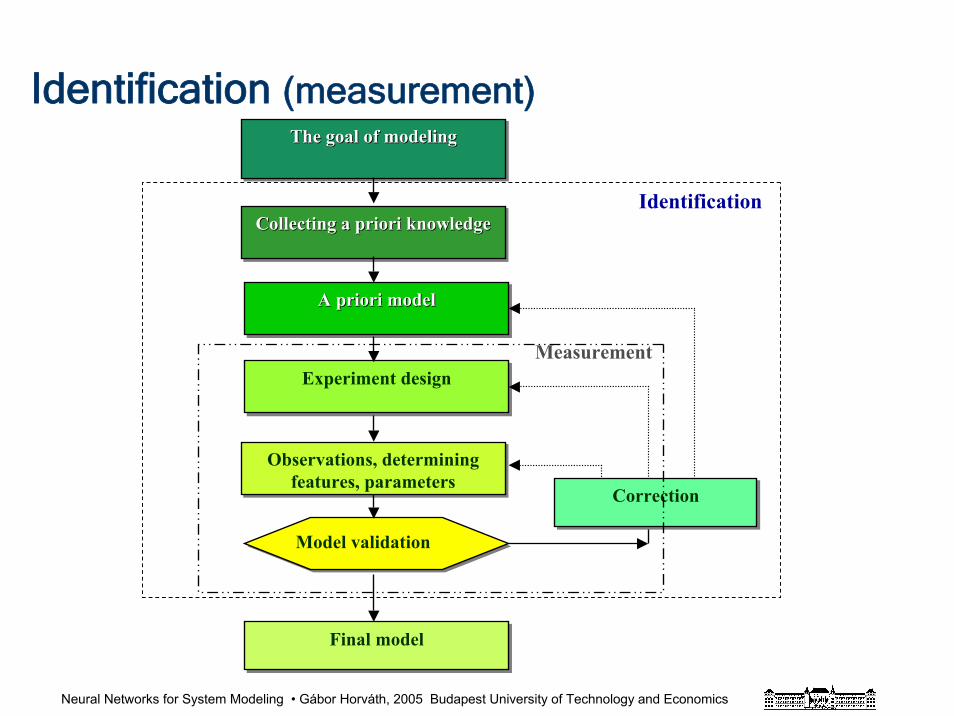
Identification (measurement)The goal of modelingThe goal of modelingThe goal of modeling
Collecting a priori knowledgeCollecting a priori knowledgeCollecting a priori knowledge
A priori modelA priori modelA priori model
Experiment designExperiment design
Observations, determiningfeatures, parameters
Observations, determiningfeatures, parameters
Model validationModel validation
Final modelFinal model
CorrectionCorrection
Measurement
Identification
Neural Networks for System Modeling • Gábor Horváth, 2005 Budapest University of Technology and Economics
• Based on the system characteristics
• Based on the modeling approach
• Based on the a priori information
Model classes
Neural Networks for System Modeling • Gábor Horváth, 2005 Budapest University of Technology and Economics
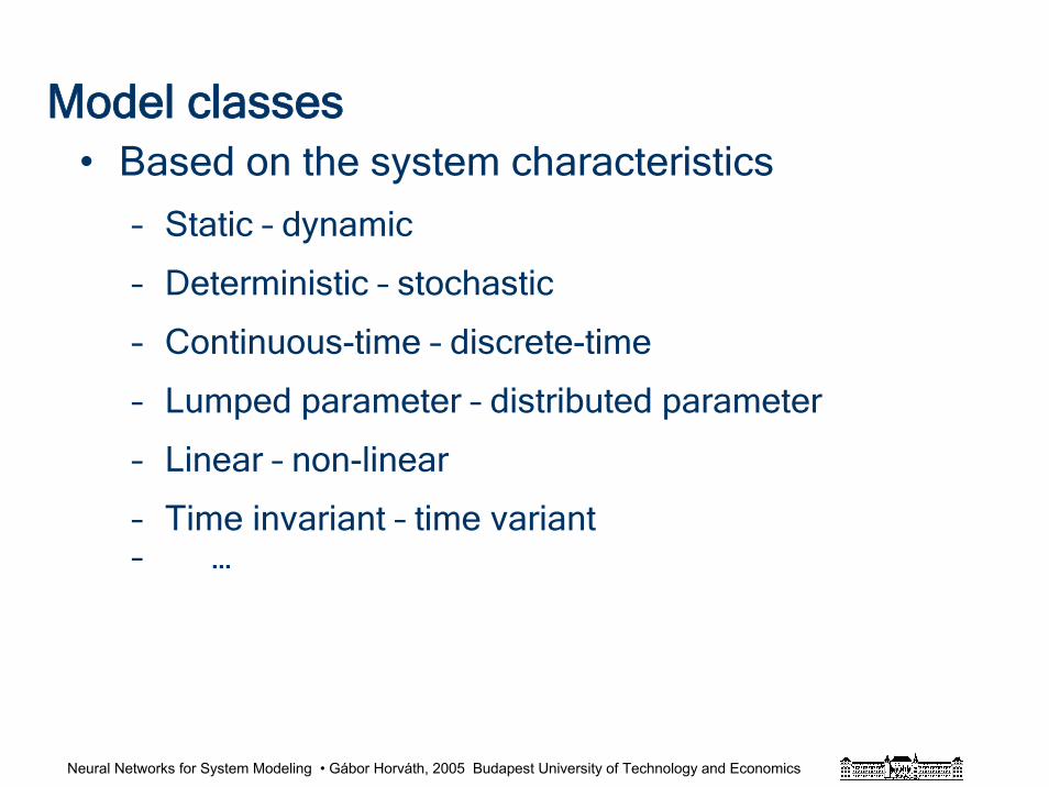
Model classes• Based on the system characteristics
– Static – dynamic
– Deterministic – stochastic
– Continuous-time – discrete-time
– Lumped parameter – distributed parameter
– Linear – non-linear
– Time invariant – time variant – …
Neural Networks for System Modeling • Gábor Horváth, 2005 Budapest University of Technology and Economics
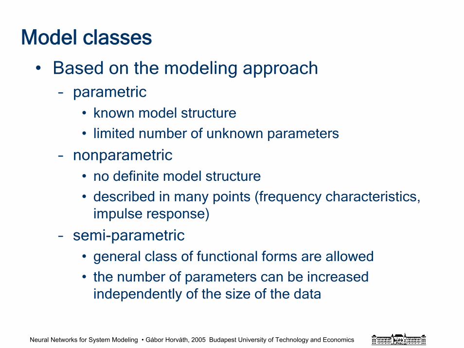
Model classes
• Based on the modeling approach– parametric
• known model structure
• limited number of unknown parameters
– nonparametric• no definite model structure
• described in many points (frequency characteristics, impulse response)
– semi-parametric• general class of functional forms are allowed
• the number of parameters can be increased independently of the size of the data
Neural Networks for System Modeling • Gábor Horváth, 2005 Budapest University of Technology and Economics
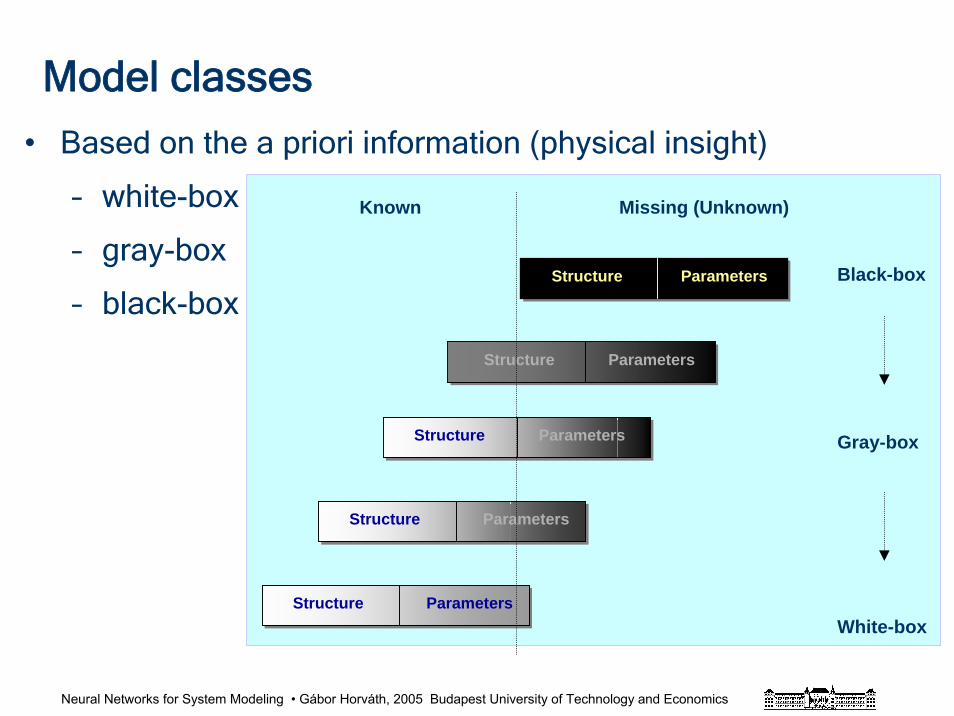
Model classes
• Based on the a priori information (physical insight)
– white-box
– gray-box
– black-boxBlack-box
White-box
Structure ParametersStructure Parameters
Structure ParametersStructure Parameters
Structure ParametersStructure Parameters
Structure ParametersStructure Parameters Gray-box
Structure ParametersStructure Parameters
Known Missing (Unknown)
Neural Networks for System Modeling • Gábor Horváth, 2005 Budapest University of Technology and Economics
Identification
• Main steps— collect information
– model set selection
– experiment design and data collection
– determine model parameters (estimation)
– model validation
Neural Networks for System Modeling • Gábor Horváth, 2005 Budapest University of Technology and Economics
Identification• Collect information
– physical insight (a priori information)
understanding the physical behaviour– only observations or experiments can be designed – application
• what operating conditions– one operating point– a large range of different conditions
• what purpose– scientific
basic research – engineering
to study the behavior of a system, to detect faults, to design control systems,etc.
Neural Networks for System Modeling • Gábor Horváth, 2005 Budapest University of Technology and Economics
Identification
• Model set selection– static – dynamic
– linear – non-linear
– non-linear
• linear - in - the - parameters
• non-linear - in - the - parameters
– white-box – black-box
– parametric – non-parametric
Neural Networks for System Modeling • Gábor Horváth, 2005 Budapest University of Technology and Economics
Identification
• Model structure selection
– known model structure (available a priori
information)
– no physical insights, general model structure
• general rule: always use as simple model as
possible (Occam’s razor)
– linear
– feed-forward
•
••
Neural Networks for System Modeling • Gábor Horváth, 2005 Budapest University of Technology and Economics
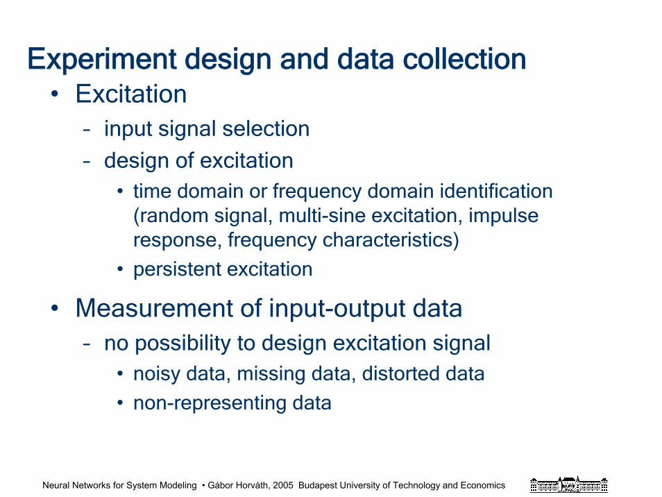
Experiment design and data collection• Excitation
– input signal selection
– design of excitation• time domain or frequency domain identification
(random signal, multi-sine excitation, impulse response, frequency characteristics)
• persistent excitation
• Measurement of input-output data – no possibility to design excitation signal
• noisy data, missing data, distorted data
• non-representing data
Neural Networks for System Modeling • Gábor Horváth, 2005 Budapest University of Technology and Economics
Excitation
• Step function
• Random signal (autoregressive moving average (ARMA) process)
• Pseudorandom binary sequence
• Multisine
Neural Networks for System Modeling • Gábor Horváth, 2005 Budapest University of Technology and Economics
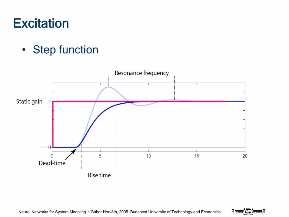
Excitation
• Step function
Neural Networks for System Modeling • Gábor Horváth, 2005 Budapest University of Technology and Economics
Excitation
• Random signal (autoregressive moving
average (ARMA) process)
– obtained by filtering white noise
– filter is selected according to the desired
frequency characteristic
– an ARMA(p,q) process can be characterized
• in time domain
• in lag (correlation) domain
• in frequency domain
Neural Networks for System Modeling • Gábor Horváth, 2005 Budapest University of Technology and Economics
Excitation
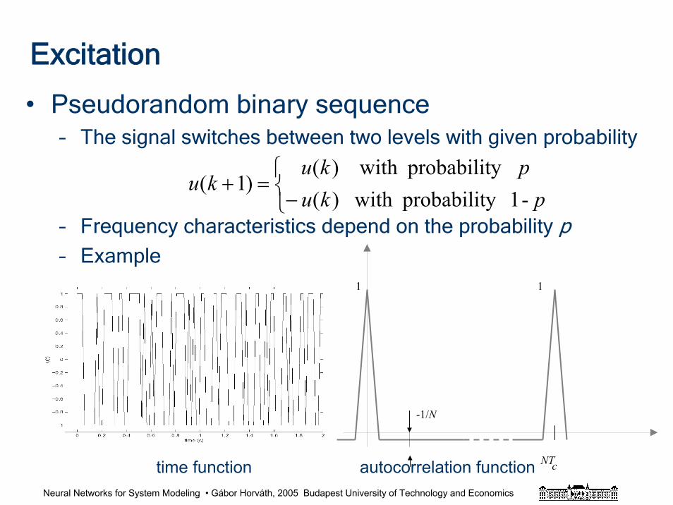
• Pseudorandom binary sequence– The signal switches between two levels with given probability
– Frequency characteristics depend on the probability p– Example
-1y probabilit with)(
y probabilit with)()1(
⎩⎨⎧
−=+
pkupku
ku
1 1
-1/N
NTctime function autocorrelation function
Neural Networks for System Modeling • Gábor Horváth, 2005 Budapest University of Technology and Economics
Excitation
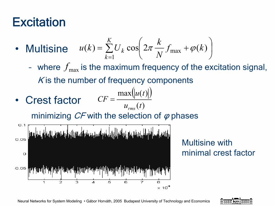
• Multisine
– where is the maximum frequency of the excitation signal,
K is the number of frequency components
• Crest factorminimizing CF with the selection of φ phases
∑=
⎟⎠⎞
⎜⎝⎛ +=
K
kk kf
NkUku
1max )(2cos)( ϕπ
( ))()(max
tutu
CFrms
=
maxf
Multisine with minimal crest factor
Neural Networks for System Modeling • Gábor Horváth, 2005 Budapest University of Technology and Economics
Excitation
• Persistent excitation– The excitation signal must be „rich” enough to
excite all modes of the system – Mathematical formulation of persistent excitation
• For linear systems– Input signal should excite all frequencies,
amplitude not so important
• For nonlinear systems– Input signal should excite all frequencies and
amplitudes– Input signal should sample the full regressor
space
Neural Networks for System Modeling • Gábor Horváth, 2005 Budapest University of Technology and Economics
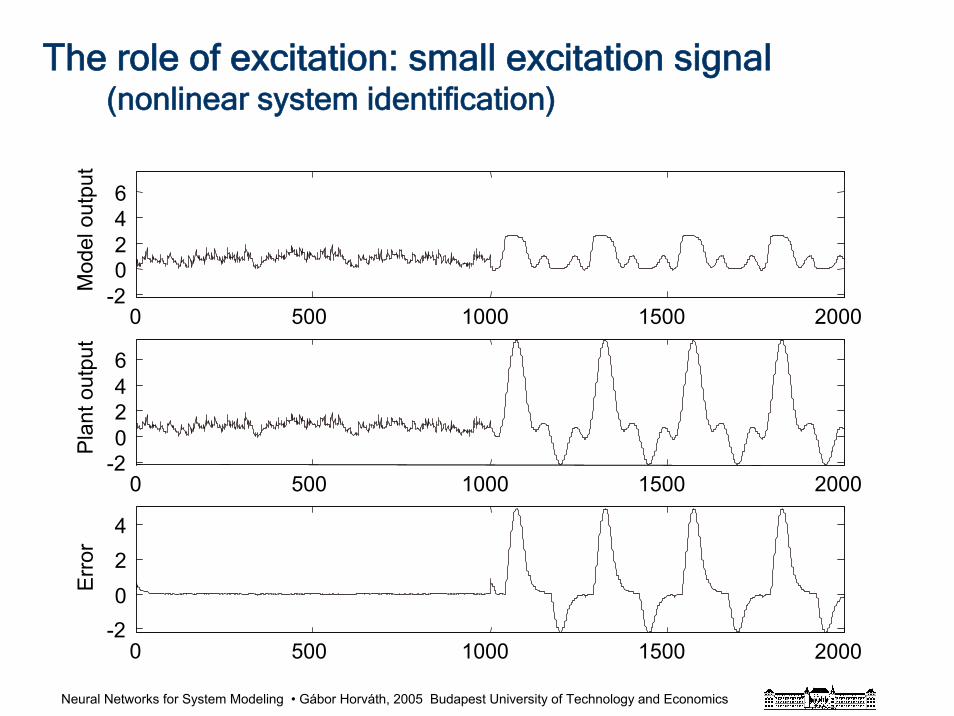
The role of excitation: small excitation signal(nonlinear system identification)
0 500 1000 1500 2000-20246
Mod
elou
tput
0 500 1000 1500 2000-20246
Plan
tout
put
0 500 1000 1500 2000-2024
Erro
r
Neural Networks for System Modeling • Gábor Horváth, 2005 Budapest University of Technology and Economics
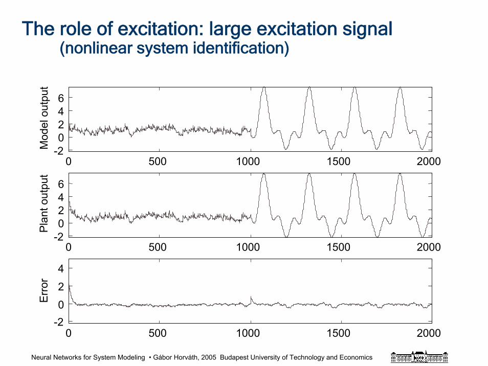
The role of excitation: large excitation signal(nonlinear system identification)
0 500 1000 1500 2000-20246
Mod
elou
tput
0 500 1000 1500 2000-20246
Plan
tout
put
0 500 1000 1500 2000-2024
Erro
r
Neural Networks for System Modeling • Gábor Horváth, 2005 Budapest University of Technology and Economics
Modeling (some examples)
• Resistor modeling
• Model of a duct (an anti-noise problem)
• Model of a steel converter (model of a
complex industrial process)
• Model of a signal (time series modeling)
Neural Networks for System Modeling • Gábor Horváth, 2005 Budapest University of Technology and Economics
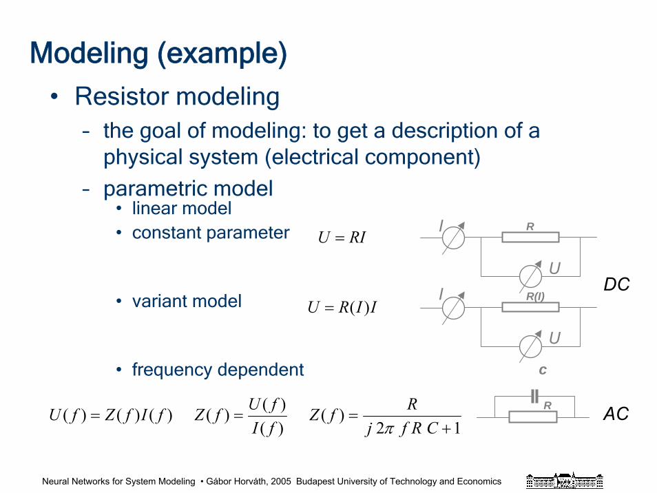
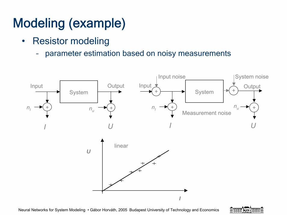
Modeling (example)
• Resistor modeling– the goal of modeling: to get a description of a
physical system (electrical component)
– parametric model• linear model• constant parameter
• variant model
• frequency dependent c
DC
12)(
)()()()()()(
+===
CRfjRfZ
fIfUfZfIfZfU
π
RRIU =
I
UI R(I)
IIRU )(=
U
R AC
Neural Networks for System Modeling • Gábor Horváth, 2005 Budapest University of Technology and Economics
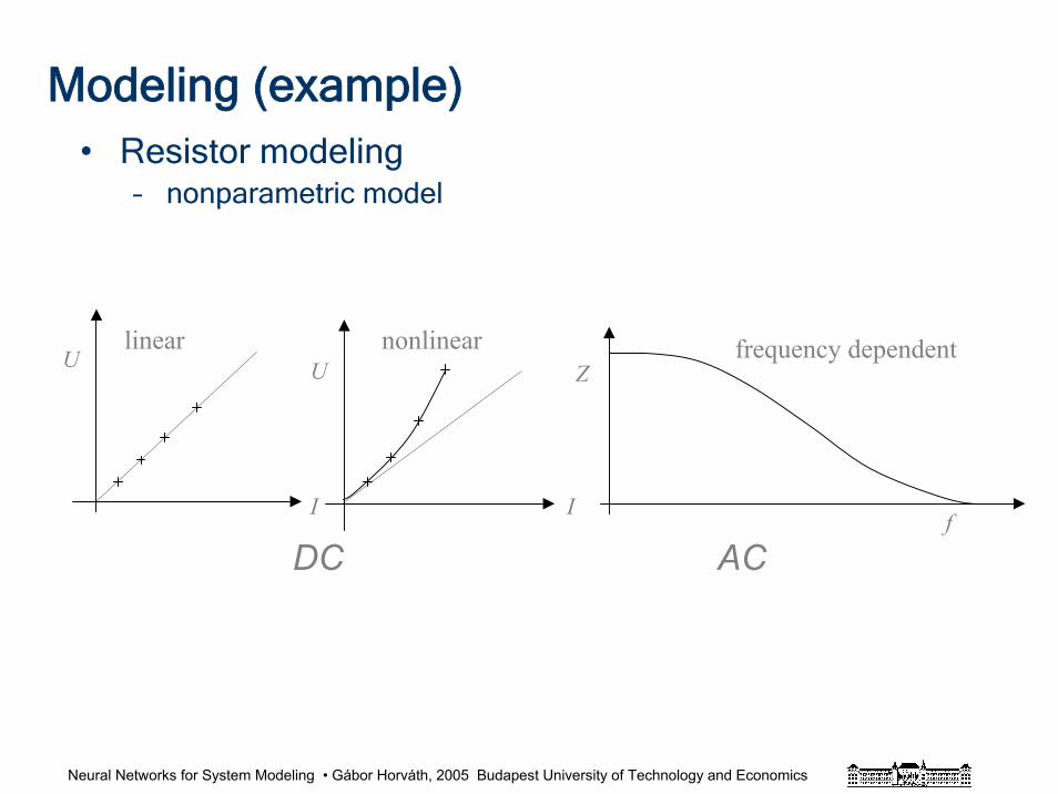
Modeling (example)• Resistor modeling
– nonparametric model
Z
fI
Unonlinear
I
Ulinear
AC
frequency dependent
DC
Neural Networks for System Modeling • Gábor Horváth, 2005 Budapest University of Technology and Economics
Modeling (example)• Resistor modeling
– parameter estimation based on noisy measurements
I
Ulinear
OutputSystem
+ +nunI
Input
I U
System
nu
OutputInput
+nI
I
+
U
+
System noise
Measurement noise
+
Input noise
Neural Networks for System Modeling • Gábor Horváth, 2005 Budapest University of Technology and Economics
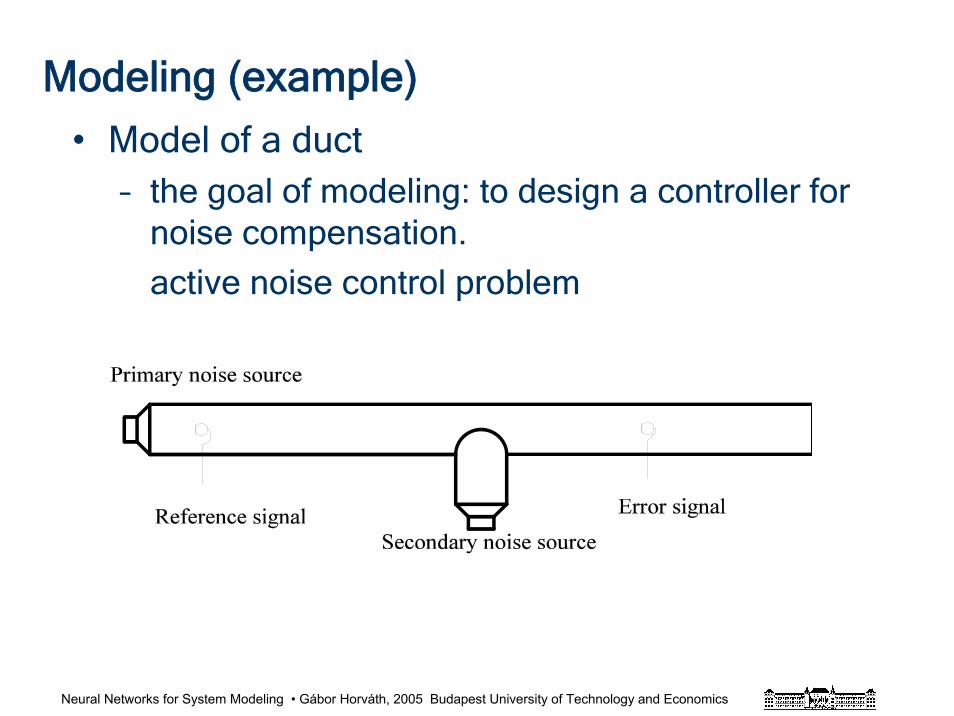
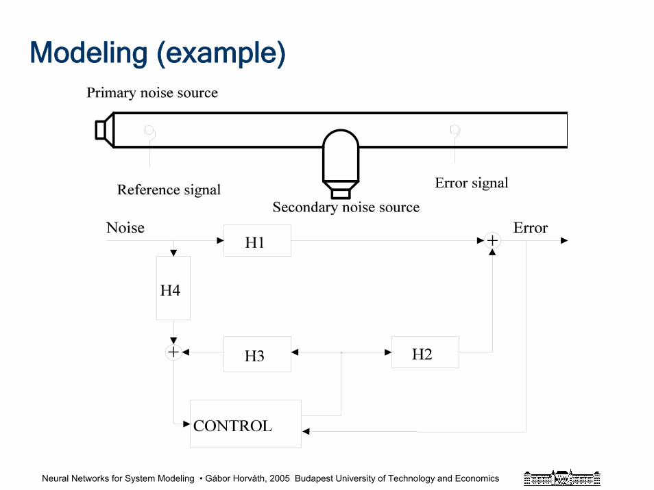
Modeling (example)
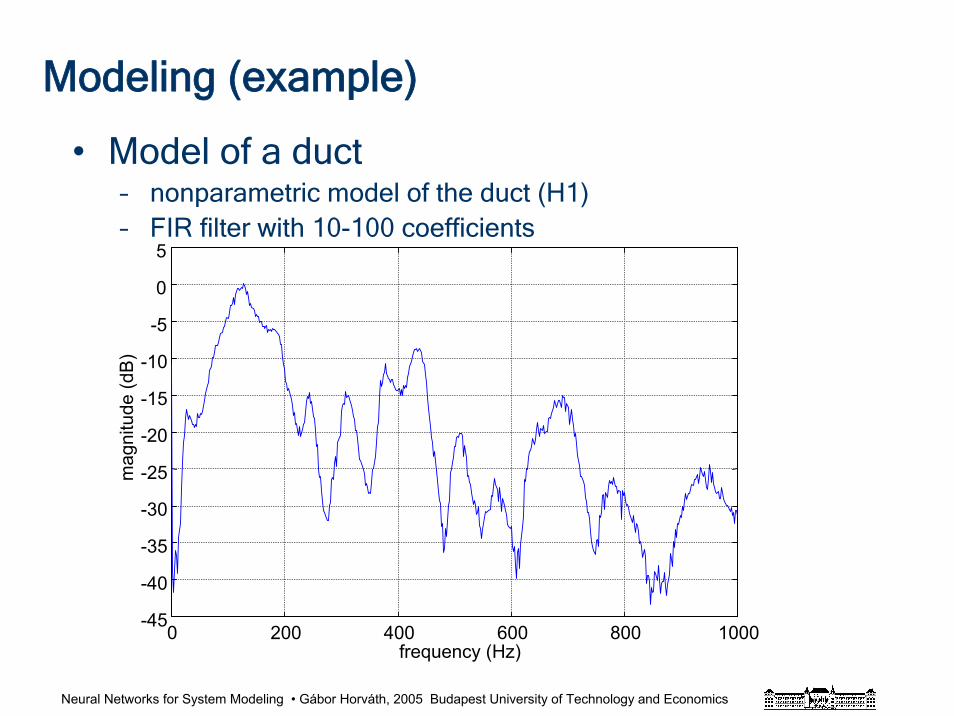
• Model of a duct– the goal of modeling: to design a controller for
noise compensation.
active noise control problem
Neural Networks for System Modeling • Gábor Horváth, 2005 Budapest University of Technology and Economics
Modeling (example)
Neural Networks for System Modeling • Gábor Horváth, 2005 Budapest University of Technology and Economics
Modeling (example)
• Model of a duct – physical modeling: general knowledge about acoustical
effects; propagation of sound, etc.
– no physical insight. Input: sound pressure, output: sound pressure
– what signals: stochastic or deterministic: periodic, non-periodic, combined, etc.
– what frequency range
– time invariant or not
– fixed solution, adaptive solution. Model structure is fixed, model parameters are estimated and adjusted: adaptive solution
Neural Networks for System Modeling • Gábor Horváth, 2005 Budapest University of Technology and Economics
Modeling (example)
• Model of a duct– nonparametric model of the duct (H1)– FIR filter with 10-100 coefficients
0 200 400 600 800 1000-45
-40
-35
-30
-25
-20
-15
-10
-5
0
5
frequency (Hz)
mag
nitu
de(d
B)
Neural Networks for System Modeling • Gábor Horváth, 2005 Budapest University of Technology and Economics
Modeling (example)
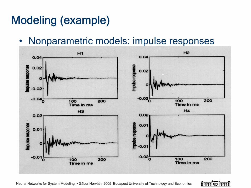
• Nonparametric models: impulse responses
Neural Networks for System Modeling • Gábor Horváth, 2005 Budapest University of Technology and Economics
Modeling (example)
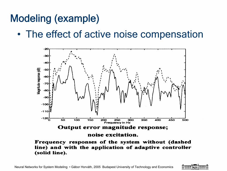
• The effect of active noise compensation

Neural Networks for System Modeling • Gábor Horváth, 2005 Budapest University of Technology and Economics
Modeling (example)
• Model of a steel converter (LD converter)

Neural Networks for System Modeling • Gábor Horváth, 2005 Budapest University of Technology and Economics
Modeling (example)
• Model of a steel converter (LD converter)– the goal of modeling: to control steel-making
process to get predetermined quality steel
– physical insight: • complex physical-chemical process with many inputs
• heat balance, mass balance
• many unmeasurable (input) variables (parameters)
– no physical insight: • there are input-output measurement data
– no possibility to design input signal, no possibility to cover the whole range of operation
Neural Networks for System Modeling • Gábor Horváth, 2005 Budapest University of Technology and Economics
Modeling (example)
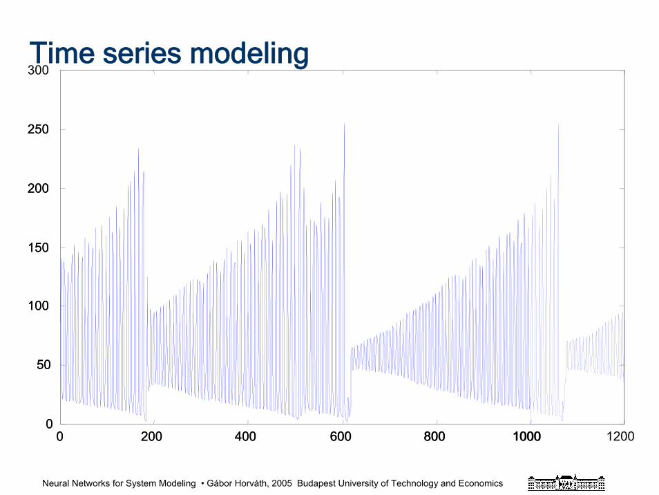
• Time series modeling– the goal of modeling: to predict the future
behaviour of a signal (forecasting)• financial time series
• physical phenomena e.g. sunspot activity
• electrical load prediction
• an interesting project: Santa Fe competition
• etc.
– signal modeling = system modeling
Neural Networks for System Modeling • Gábor Horváth, 2005 Budapest University of Technology and Economics
Time series modeling
0 200 400 600 800 10000
50
100
150
200
250
0 200 400 600 800 1000 12000
50
100
150
200
250
300
Neural Networks for System Modeling • Gábor Horváth, 2005 Budapest University of Technology and Economics
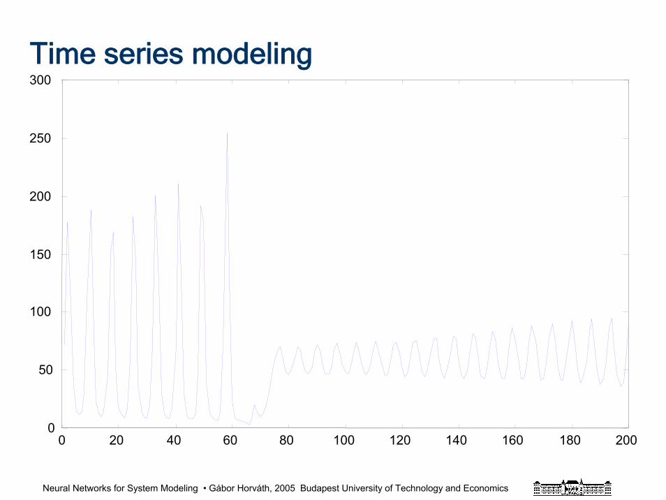
Time series modeling
0 20 40 60 80 100 120 140 160 180 2000
50
100
150
200
250
300
Neural Networks for System Modeling • Gábor Horváth, 2005 Budapest University of Technology and Economics
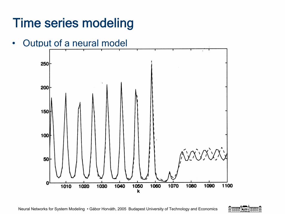
Time series modeling
• Output of a neural model
Neural Networks for System Modeling • Gábor Horváth, 2005 Budapest University of Technology and Economics
References and further readingsBox, G.E.P and Jenkins, G.M: “Time Series Analysis: Forecasting and Control”, Revised Edition,
Holden Day, 1976Eykhoff, P. “System Identification, Parameter and State Estimation”, Wiley, New York, 1974.Goodwin, G.C. and R. L. Payne, “Dynamic System Identification”, Academic Press, New York, 1977.Horváth, G. “Neural Networks in Systems Identification”, (Chapter 4. in: S. Ablameyko, L. Goras, M.
Gori and V. Piuri (Eds.) Neural Networks in Measurement Systems) NATO ASI, IOS Press, pp. 43-78. 2002.
Horváth, G., Dunay, R.: "Application of Neural Networks to Adaptive Filtering for Systems with External Feedback Paths." Proc. of The International Conferenace on Signal Processing Application and Technology. Vol. II. pp. 1222-1227. Dallas, Tx. 1994.
Ljung, L. “System Identification - Theory for the User”. Prentice-Hall, N.J. 2nd edition, 1999.Pintelon R. and Schoukens, J. “System Identification. A Frequency Domain Approach”, IEEE Press,
New York, 2001.Pataki, B., Horváth, G., Strausz, Gy. and Talata, Zs. "Inverse Neural Modeling of a Linz-Donawitz
Steel Converter" e & i Elektrotechnik und Informationstechnik, Vol. 117. No. 1. 2000. pp. 13-17.Rissanen, J. “Modelling by Shortest Data Description”, Automatica, Vol. 14. pp. 465-471, 1978.Sjöberg, J., Q. Zhang, L. Ljung, A. Benveniste, B. Delyon, P.-Y. Glorennec, H. Hjalmarsson, and A.
Juditsky: "Non-linear Black-box Modeling in System Identification: a Unified Overview",Automatica, 31:1691-1724, 1995.
Söderström, T. and P. Stoica, “System Indentification”, Prentice Hall, Englewood Cliffs, NJ. 1989.Weigend,. A.S and N.A Gershenfeld "Forecasting the Future and Understanding the Past" Vol.15.
Santa Fe Institute Studies in the Science of Complexity, Reading, MA. Addison-Wesley, 1994.
Neural Networks for System Modeling • Gábor Horváth, 2005 Budapest University of Technology and Economics
Identification (linear systems)
• Parametric identification (parameter estimation)
– LS estimation
– ML estimation
– Bayes estimation
• Nonparametric identification
– Transient analysis
– Correlation analysis
– Frequency analysis
Neural Networks for System Modeling • Gábor Horváth, 2005 Budapest University of Technology and Economics
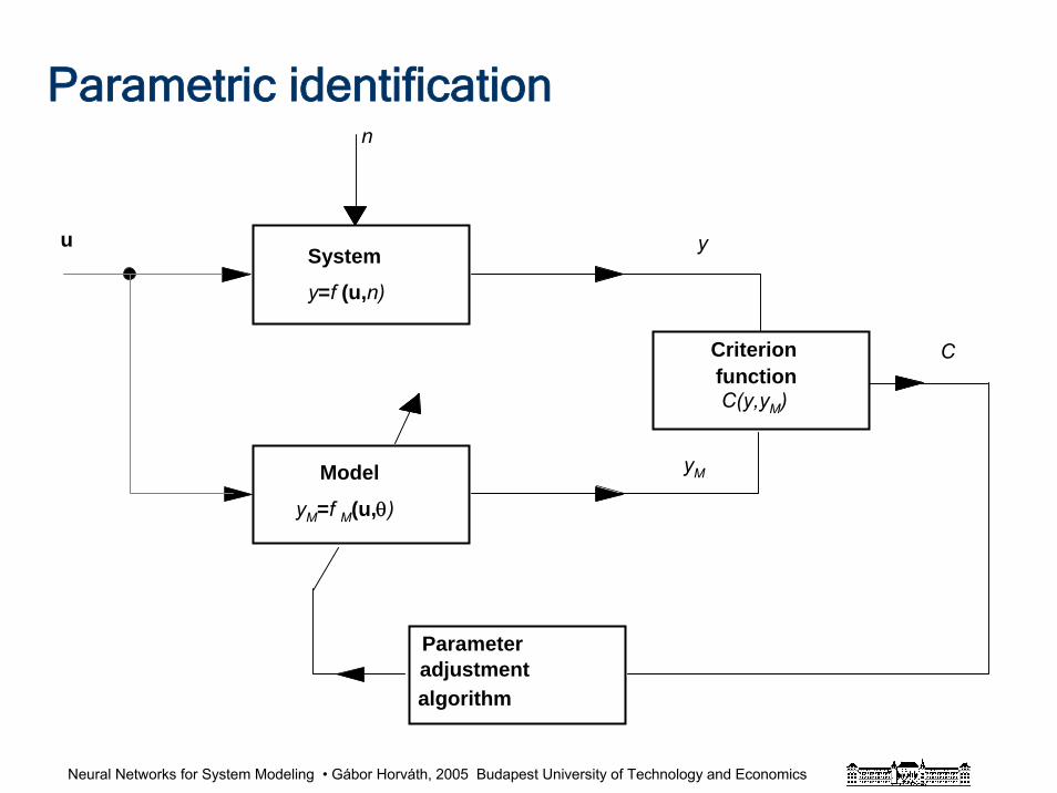
Parametric identificationn
y
yM
CCriterion
C(y,yM)
Model
Parameter
algorithm
System
function
adjustment
u
y=f (u,n)
yM=f M(u,θ)
Neural Networks for System Modeling • Gábor Horváth, 2005 Budapest University of Technology and Economics
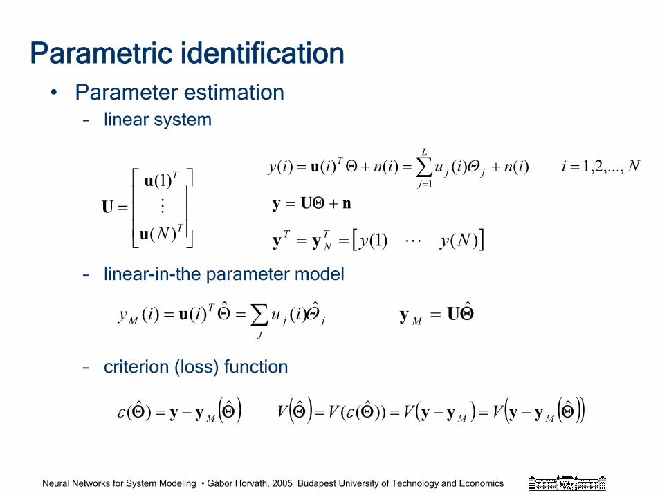
Parametric identification• Parameter estimation
– linear system
– linear-in-the parameter model
– criterion (loss) function
NiiniuiniiyL
jjj
T 1,2,..., )()()()()(1
=+=+Θ= ∑=
Θu
jj
jT
M iuiiy Θ)(ˆ)()( ∑=Θ= u
[ ])()1( NyyTN
T L== yy
nUy += Θ
⎥⎥⎥
⎦
⎤
⎢⎢⎢
⎣
⎡
=T
T
N )(
)1(
u
uU M
ΘUy =M
( ) ( ) ( )( )ΘΘΘ ˆ))ˆ((ˆMM VVVV yyyy −=−== ε( )ΘΘ ˆ)ˆ( Myy −=ε
Neural Networks for System Modeling • Gábor Horváth, 2005 Budapest University of Technology and Economics
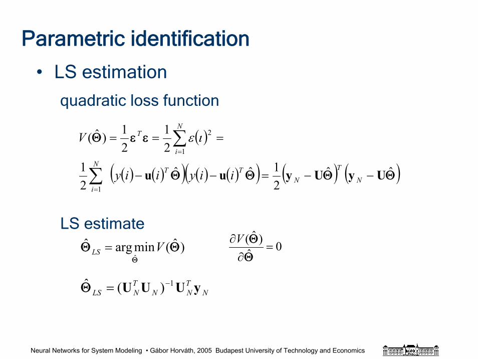
Parametric identification
• LS estimation
quadratic loss function
LS estimate
( )
( ) ( )( ) ( ) ( )( ) ( ) ( )ΘΘΘΘ
εεΘ
ˆˆ21ˆˆ
21
21
21)ˆ(
1
1
2
UyUyuu −−=−−
===
∑
∑
=
=
N
T
NTT
N
i
N
i
T
iiyiiy
V ιε
)ˆ(minargˆˆ
ΘΘΘ
VLS = 0ˆ)ˆ(
=∂
∂ΘΘV
NTNN
TNLS yUUU 1)(ˆ −=Θ
Neural Networks for System Modeling • Gábor Horváth, 2005 Budapest University of Technology and Economics
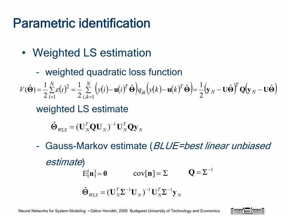
Parametric identification
• Weighted LS estimation
– weighted quadratic loss function
weighted LS estimate
– Gauss-Markov estimate (BLUE=best linear unbiased
estimate)
NTNN
TNWLS yUUU 111 )(ˆ −−−= ΣΣΘ
NTNN
TNWLS QyUQUU 1)(ˆ −=Θ
( ) ( ) ( )( ) ( ) ( )( ) ( ) ( )ΘUyQΘUyΘuΘuΘ ˆˆ21ˆˆ
21
21)ˆ(
1,1
2 −−=−−∑=∑===
NT
NT
ikTN
ki
N
ikkyqiiyV ιε
1−= ΣQ 0n =E Σ]cov[ =n
Neural Networks for System Modeling • Gábor Horváth, 2005 Budapest University of Technology and Economics
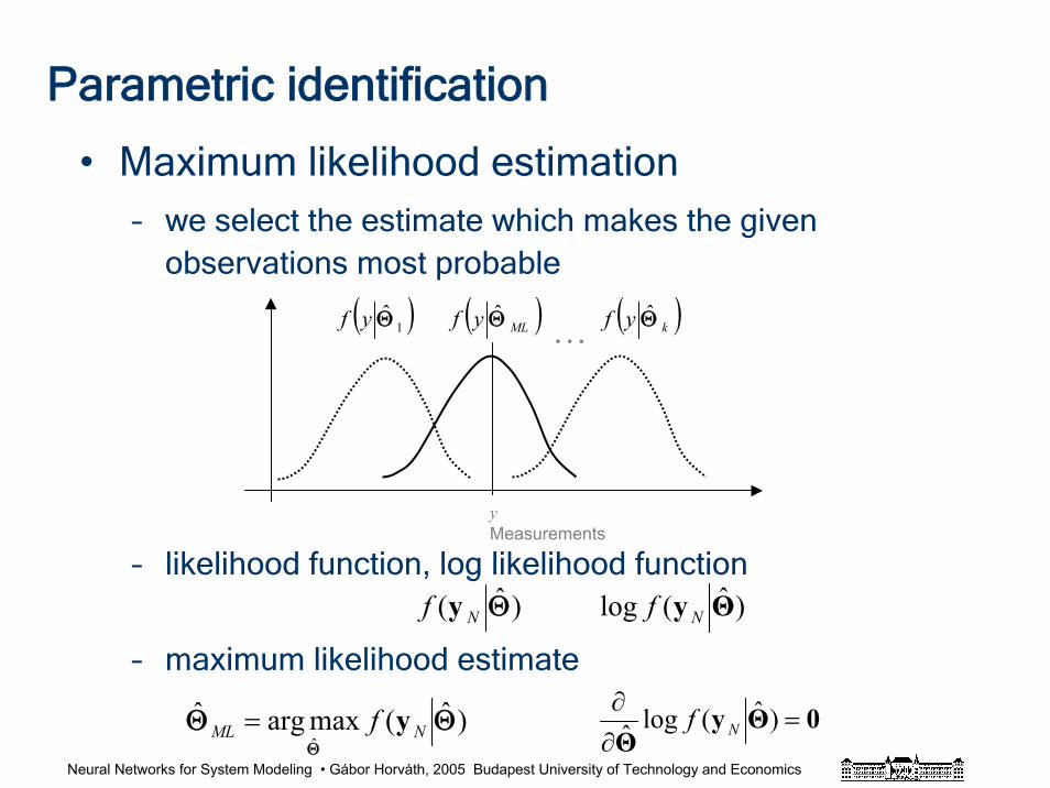
Parametric identification
• Maximum likelihood estimation– we select the estimate which makes the given
observations most probable
– likelihood function, log likelihood function
– maximum likelihood estimate
)ˆ(maxargˆˆ
ΘΘΘ
NML f y=
y Measurements
( )1Θyf ( )MLyf Θ ( )kyf Θ…
)ˆ( ΘNf y )ˆ(log Θy Nf
0ΘyΘ
=∂∂ )ˆ(logˆ Nf

Neural Networks for System Modeling • Gábor Horváth, 2005 Budapest University of Technology and Economics
Parametric identification• Properties of ML estimates
– consistency
– asymptotic normality
– asymptotic efficiency: the variance reaches Cramer-Rao
lower bound
– Gauss-Markov if Gaussian
( ) 0 anyfor 0ˆlim >=>−∞→
εεΘΘ NMLNP
converges to a normal random variable as N→∞)(ˆ
NMLΘ
( ) 1
2
2
)(
ln)ˆvar(lim
−
∞→ ⎟⎟⎠
⎞⎜⎜⎝
⎛
⎭⎬⎫
⎩⎨⎧
∂∂
−=−Θ
ΘΘΘ
yfENMLN
)ˆ( ΘNf y
Neural Networks for System Modeling • Gábor Horváth, 2005 Budapest University of Technology and Economics
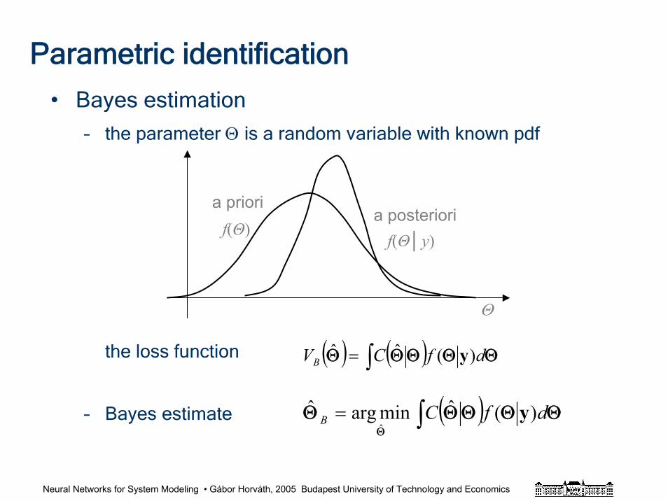
Parametric identification
• Bayes estimation
– the parameter Θ is a random variable with known pdf
the loss function
– Bayes estimate
a prioria posteriori
f(Θ)f(Θy)
Θ
( ) ( ) ΘΘΘΘΘ dfCVB )(ˆˆ y∫=
( ) ΘΘΘΘΘΘ
dfCB )(ˆminargˆˆ
y∫=
Neural Networks for System Modeling • Gábor Horváth, 2005 Budapest University of Technology and Economics
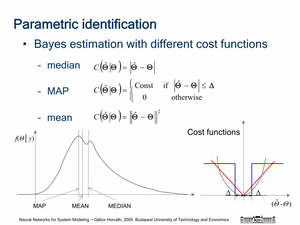
Parametric identification
• Bayes estimation with different cost functions
– median
– MAP
– mean
( ) ΘΘΘΘ −= ˆˆC
( ) 2ˆˆ ΘΘΘΘ −=C
( )⎪⎩
⎪⎨⎧ ≤−=
otherwise0
ˆifConstˆ ΔΘΘΘΘC
MAP MEAN MEDIAN
f(Θy)Cost functions
)-ˆ( ΘΘΔ Δ
Neural Networks for System Modeling • Gábor Horváth, 2005 Budapest University of Technology and Economics
Parametric identification
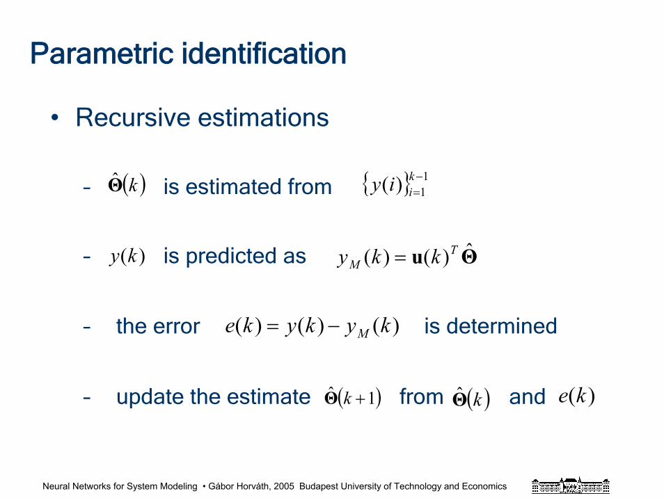
• Recursive estimations
– is estimated from
– is predicted as
– the error is determined
– update the estimate from and
( )kΘ 11)( −
=kiiy
)(ky Θu ˆ)()( TM kky =
)()()( kykyke M−=
( )1ˆ +kΘ ( )kΘ )(ke
Neural Networks for System Modeling • Gábor Horváth, 2005 Budapest University of Technology and Economics
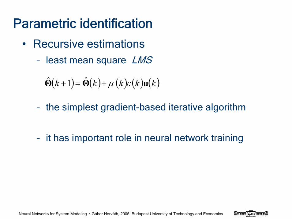
Parametric identification
• Recursive estimations– least mean square LMS
– the simplest gradient-based iterative algorithm
– it has important role in neural network training
( ) ( ) ( ) ( ) ( )kkkkk uΘΘ εμ+=+ ˆ1ˆ
Neural Networks for System Modeling • Gábor Horváth, 2005 Budapest University of Technology and Economics
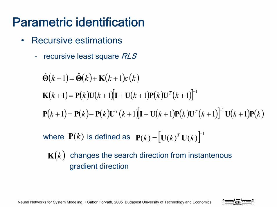
Parametric identification• Recursive estimations
– recursive least square RLS
where is defined as
changes the search direction from instantenous
gradient direction
( ) ( ) ( ) ( )kkkk ε1ˆ1ˆ ++=+ KΘΘ
( ) ( ) ( ) ( ) ( ) ( )[ ] 11111 −++++=+ kkkkkk TUPUIUPK
( ) ( ) ( ) ( ) ( ) ( ) ( )[ ] ( ) ( )kkkkkkkkk TT PUUPUIUPPP 11111 1+++++−=+
−
[ ] 1)()()(
−= kkk T UUP)(kP
( )kK
Neural Networks for System Modeling • Gábor Horváth, 2005 Budapest University of Technology and Economics
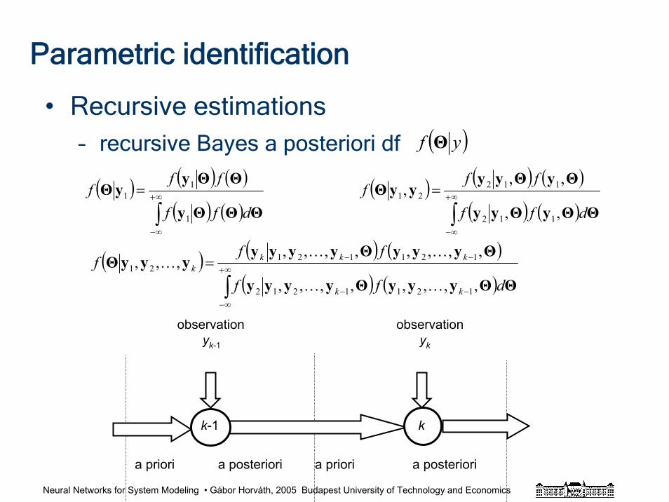
Parametric identification
• Recursive estimations– recursive Bayes a posteriori df
a priori a posteriori a priori a posteriori
observation observationyk-1 yk
k-1 k
( )yf Θ
( ) ( ) ( )
( ) ( )∫∞+
∞−
=ΘΘΘy
ΘΘyyΘ
dff
fff
1
11 ( ) ( ) ( )
( ) ( )∫∞+
∞−
=ΘΘyΘyy
ΘyΘyyyyΘ
dff
fff
,,
,,,
112
11221
( ) ( ) ( )
( ) ( )∫∞+
∞−−−
−−=ΘΘyyyΘyyyy
ΘyyyΘyyyyyyyΘ
dff
fff
kk
kkkk
,,,,,,,,
,,,,,,,,,,,
1211212
12112121
KK
KKK
Neural Networks for System Modeling • Gábor Horváth, 2005 Budapest University of Technology and Economics
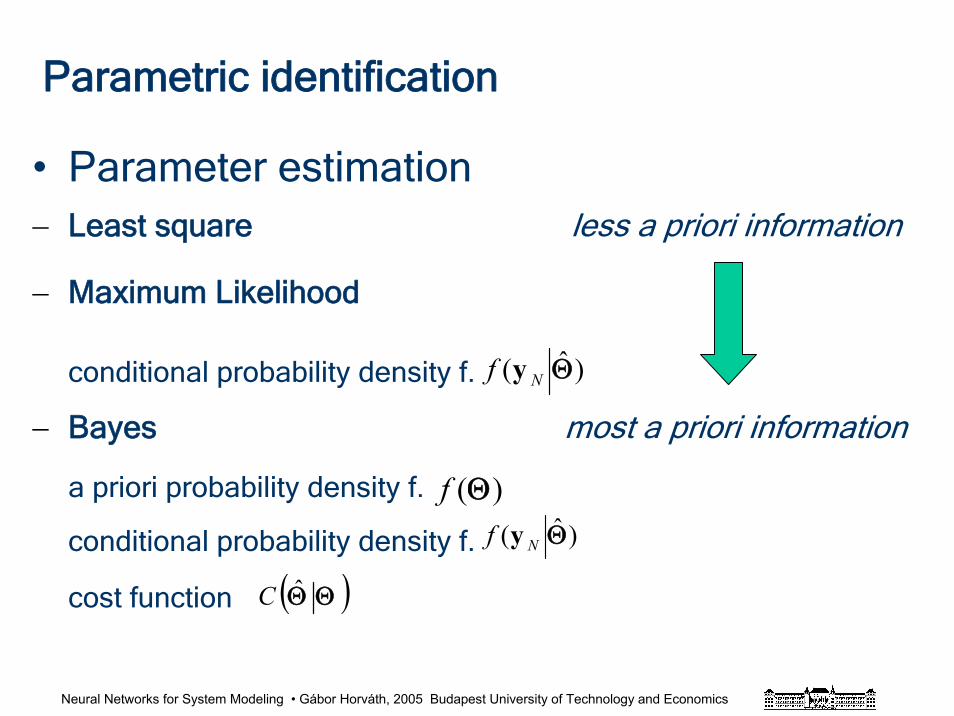
Parametric identification
• Parameter estimation− Least square less a priori information
− Maximum Likelihood
conditional probability density f.
− Bayes most a priori information
a priori probability density f.
conditional probability density f.
cost function
)ˆ( ΘNf y
( )ΘΘC
)(Θf
)ˆ( ΘNf y
Neural Networks for System Modeling • Gábor Horváth, 2005 Budapest University of Technology and Economics
Non-parametric identification
• Frequency-domain analysis
– frequency characteristic, frequency response
– spectral analysis
• Time-domain analysis
– impulse response
– step response
– correlation analysis
• These approaches are for linear dynamical systems
Neural Networks for System Modeling • Gábor Horváth, 2005 Budapest University of Technology and Economics
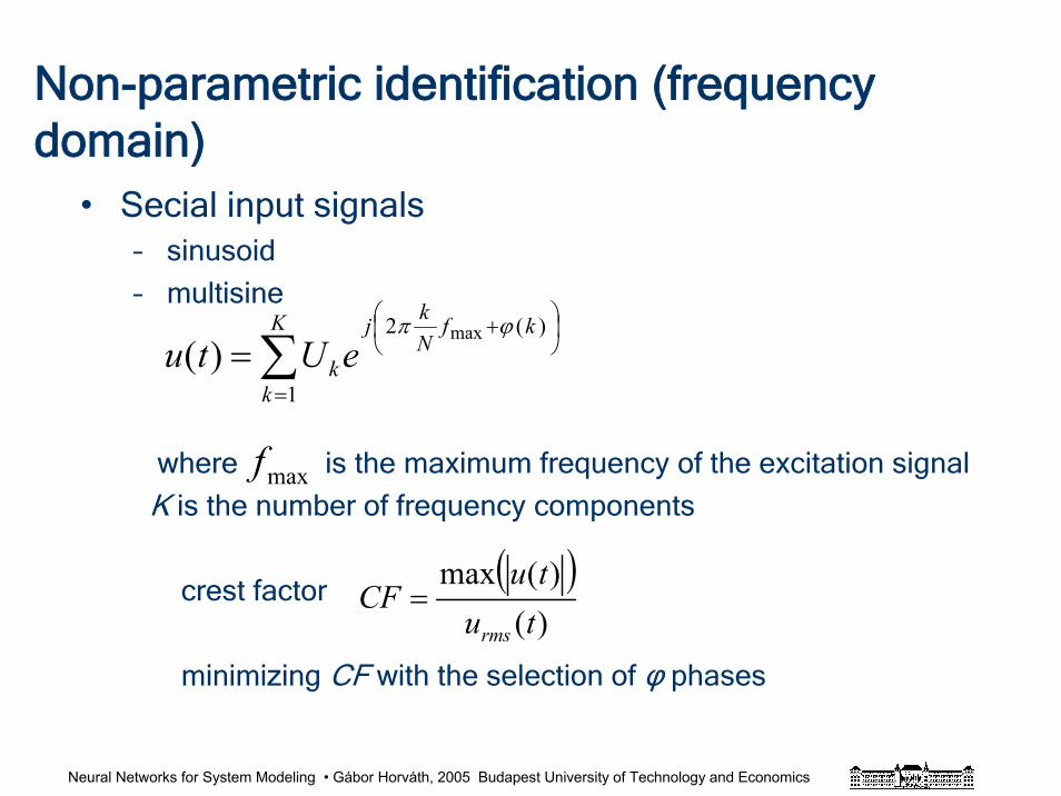
Non-parametric identification (frequency domain)
• Secial input signals– sinusoid
– multisine
where is the maximum frequency of the excitation signal
K is the number of frequency components
crest factor
minimizing CF with the selection of φ phases
∑=
⎟⎠⎞
⎜⎝⎛ +
=K
k
kfNkj
keUtu1
)(2 max)(
ϕπ
maxf
( ))()(max
tutu
CFrms
=
Neural Networks for System Modeling • Gábor Horváth, 2005 Budapest University of Technology and Economics
Non-parametric identification (frequency domain)
• Frequency response
– Power density spectrum, periodogram
– Calculation of periodogram
– Effect of finite registration length
– Windowing (smoothing)
Neural Networks for System Modeling • Gábor Horváth, 2005 Budapest University of Technology and Economics
References and further readingsEykhoff, P. System Identification, Parameter and State Estimation, Wiley, New York, 1974.
Ljung, L. ”System Identification - Theory for the User” Prentice-Hall, N.J. 2nd edition, 1999.
Goodwin, G.C. and R.L. Payne, Dynamic System Identification, Academic Press, New York, 1977.
Rissanen, J. “Stochastic Complexity in Statistical Inquiry”, Series in Computer Science”. Vol. 15 World Scientific, 1989.
Sage, A.P. and J.L. Melsa, Estimation Theory with Application to Communications and Control, McGraw-Hill, New York, 1971.
Pintelon, R. and J. Schoukens, System Identification. A Frequency Domain Approach, IEEE Press, New York, 2001.
Söderström, T. and P. Stoica, System Indentification, Prentice Hall, Englewood Cliffs, NJ. 1989.
Van Trees, H.L. Detection Estimation and Modulation Theory, Part I. Wiley, New York, 1968.
Neural Networks for System Modeling • Gábor Horváth, 2005 Budapest University of Technology and Economics
Black box modeling
Neural Networks for System Modeling • Gábor Horváth, 2005 Budapest University of Technology and Economics
Black-box modeling
• Why do we use black-box models?
– the lack of physical insight: physical modeling is not
possible
– the physical knowledge is too complex, there are
mathematical difficulties; physical modeling is possible
in principle but not possible in practice
– there is no need for physical modeling, (only the
behaviour of the system should be modeled)
– black-box modeling may be much simpler
Neural Networks for System Modeling • Gábor Horváth, 2005 Budapest University of Technology and Economics
Black-box modeling
• Steps of black-box modeling
– select a model structure
– determine the size of the model (the number of
parameters)
– use observed (measured) data to adjust the model
(estimate the model order - the number of
parameters - and the numerical values of the
parameters)
– validate the resulted model
Neural Networks for System Modeling • Gábor Horváth, 2005 Budapest University of Technology and Economics
Black-box modeling
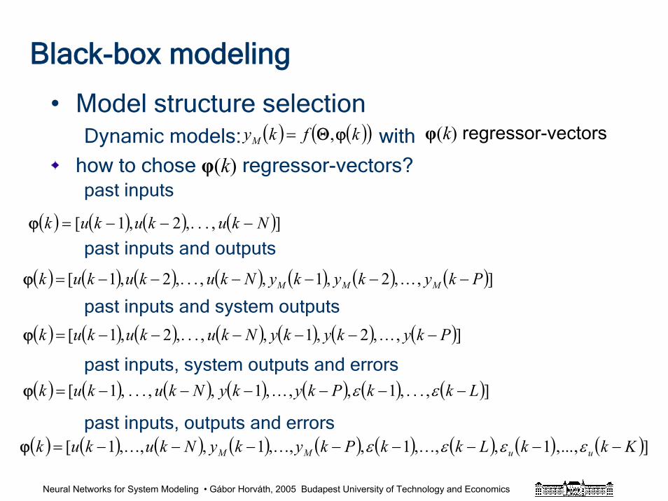
• Model structure selectionDynamic models: with
how to chose φ(k) regressor-vectors?past inputs
past inputs and outputs
past inputs and system outputs
past inputs, system outputs and errors
past inputs, outputs and errors
( ) ( )( )kfkyM ϕΘ,=
( ) ( ) ( ) ( )],...,2,1[ Nkukukuk −−−=ϕ
( ) ( ) ( ) ( ) ( ) ( ) ( )],...,2,1,,...,2,1[ PkykykyNkukukuk −−−−−−=ϕ
( ) ( ) ( ) ( ) ( ) ( ) ( )],...,2,1,,...,2,1[ PkykykyNkukukuk MMM −−−−−−=ϕ
( ) ( ) ( ) ( ) ( ) ( ) ( )],...,1,,...,1,,...,1[ LkkPkykyNkukuk −−−−−−= εεϕ
( ) ( ) ( ) ( ) ( ) ( ) ( ) ( ) ( )],...,1,,...,1,,...,1,,...,1[ KkkLkkPkykyNkukuk uuMM −−−−−−−−= εεεεϕ
φ(k) regressor-vectors
Neural Networks for System Modeling • Gábor Horváth, 2005 Budapest University of Technology and Economics
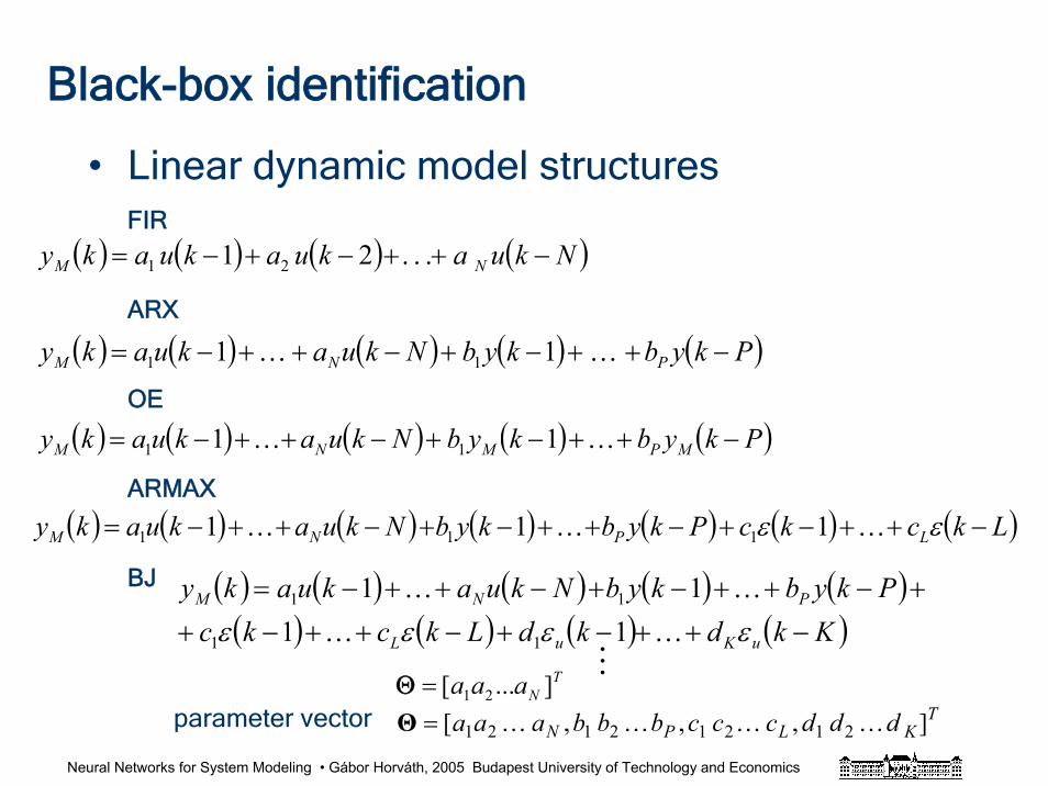
Black-box identification
• Linear dynamic model structuresFIR
ARX
OE
ARMAX
BJ
parameter vector
( ) ( ) ( ) ( )Nkuakuakuaky NM −++−+−= ...21 21
TNaaa ]...[ 21=Θ
( ) ( ) ( ) ( ) ( ) ( ) ( )LkckcPkybkybNkuakuaky LPNM −++−+−++−+−++−= εε KKK 111 111
TKLPN dddcccbbbaaa ],,,[ 21212121 KKKK=Θ
( ) ( ) ( ) ( ) ( )PkybkybNkuakuaky PNM −++−+−++−= KK 11 11
( ) ( ) ( ) ( ) ( )PkybkybNkuakuaky MPMNM −++−+−++−= KK 11 11
( ) ( ) ( ) ( ) ( )( ) ( ) ( ) ( )KkdkdLkckc
PkybkybNkuakuaky
uKuL
PNM
−++−+−++−++−++−+−++−=
εεεε KK
KK
1111
11
11
M
Neural Networks for System Modeling • Gábor Horváth, 2005 Budapest University of Technology and Economics
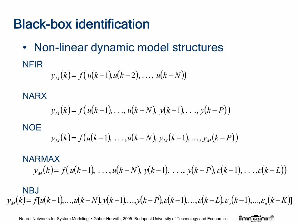
Black-box identification
• Non-linear dynamic model structuresNFIR
NARX
NOE
NARMAX
NBJ
( ) ( ) ( ) ( )( )NkukukufkyM −−−= ,...,2,1
( ) ( ) ( ) ( ) ( )( )PkykyNkukufkyM −−−−= ,...,1,,...,1
( ) ( ) ( ) ( ) ( )( )PkykyNkukufky MMM −−−−= ,...,1,,...,1
( ) ( ) ( ) ( ) ( ) ( ) ( )( )LkkPkykyNkukufkyM −−−−−−= εε ,...,1,,...,1,,...,1
( ) ( ) ( ) ( ) ( ) ( ) ( ) ( ) ( )],...,1,,...,1,,...,1,,...,1[ KkkLkkPkykyNkukufky uuM −−−−−−−−= εεεε
Neural Networks for System Modeling • Gábor Horváth, 2005 Budapest University of Technology and Economics
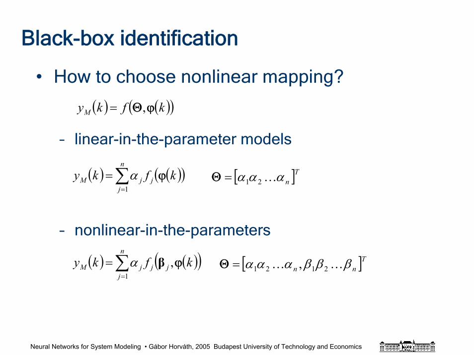
Black-box identification
• How to choose nonlinear mapping?
– linear-in-the-parameter models
– nonlinear-in-the-parameters
( ) ( )( )kfkyM ϕΘ,=
( ) ( )( )kfky j
n
jjM ϕ∑
=
=1α [ ]T
nααα K21=Θ
( ) ( )( )kfky jj
n
jjM ϕ,
1β∑
=
= α [ ]Tnn βββααα KK 2121 ,=Θ
Neural Networks for System Modeling • Gábor Horváth, 2005 Budapest University of Technology and Economics
Black-box identification
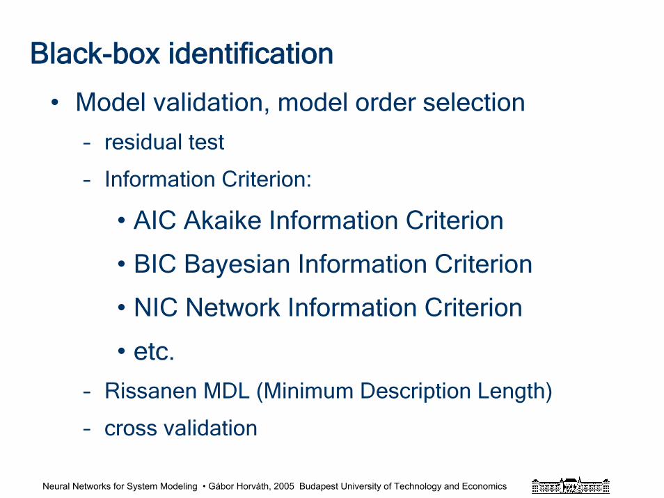
• Model validation, model order selection
– residual test
– Information Criterion:
• AIC Akaike Information Criterion
• BIC Bayesian Information Criterion
• NIC Network Information Criterion
• etc.
– Rissanen MDL (Minimum Description Length)
– cross validation
Neural Networks for System Modeling • Gábor Horváth, 2005 Budapest University of Technology and Economics
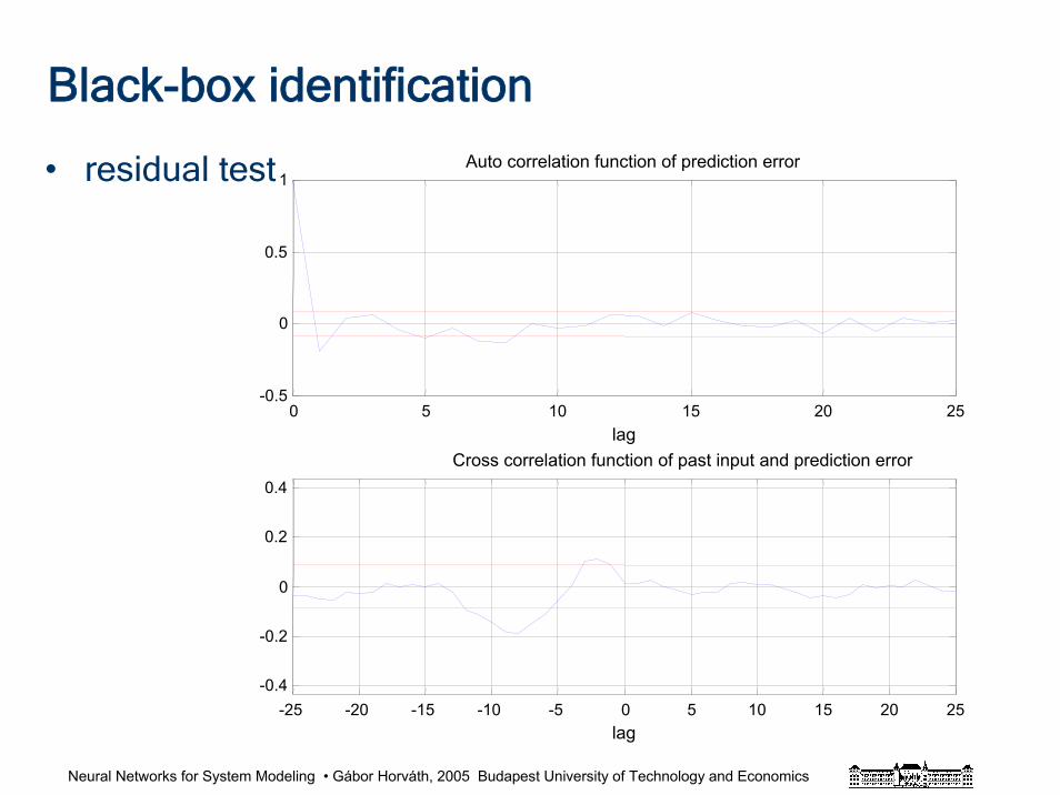
Black-box identification
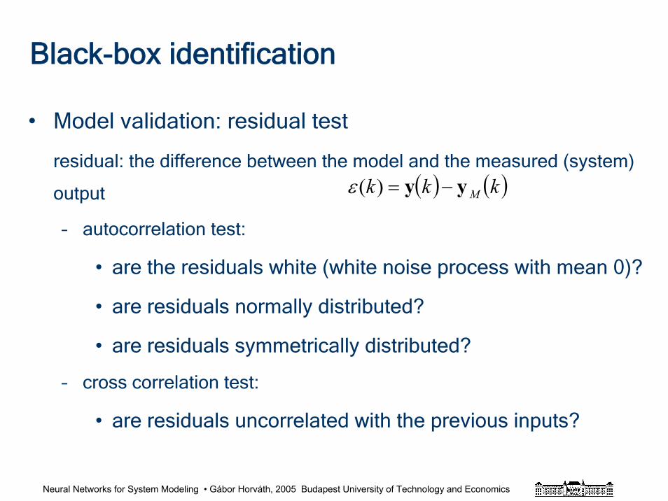
• Model validation: residual test
residual: the difference between the model and the measured (system)
output
– autocorrelation test:
• are the residuals white (white noise process with mean 0)?
• are residuals normally distributed?
• are residuals symmetrically distributed?
– cross correlation test:
• are residuals uncorrelated with the previous inputs?
( ) ( )kkk Myy −=)(ε
Neural Networks for System Modeling • Gábor Horváth, 2005 Budapest University of Technology and Economics
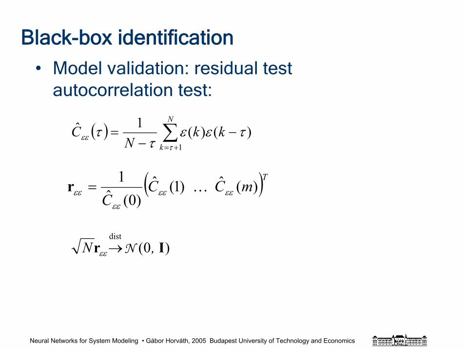
Black-box identification
• Model validation: residual test autocorrelation test:
( ) ∑+=
−−
=N
kkk
NC
1)()(1ˆ
τεε τεε
ττ
( )TmCCC
)(ˆ)1(ˆ)0(ˆ
1εεεε
εεεε K=r
)0(dist
Ir , N N→εε
Neural Networks for System Modeling • Gábor Horváth, 2005 Budapest University of Technology and Economics
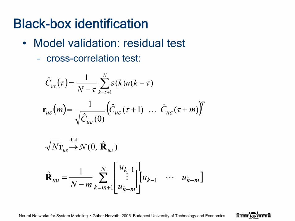
Black-box identification
• Model validation: residual test– cross-correlation test:
( ) ∑+=
−−
=N
ku kuk
NC
1
)()(1ˆτ
ε τετ
τ
( ) ( )Tuuu
u mCCC
m )(ˆ)1(ˆ)0(ˆ
1++= ττ εε
εε Kr
)ˆ0(dist
uuu , N Rr N→ε
[ ]mkk
N
mk mk
kuu uu
u
u
mN −−+= −
−∑
⎥⎥
⎦
⎤
⎢⎢
⎣
⎡
−= LM 1
1
11R
Neural Networks for System Modeling • Gábor Horváth, 2005 Budapest University of Technology and Economics
Black-box identification
• residual test
0 5 10 15 20 25-0.5
0
0.5
1
lag
Auto correlation function of prediction error
-25 -20 -15 -10 -5 0 5 10 15 20 25-0.4
-0.2
0
0.2
0.4
lag
Cross correlation function of past input and prediction error
Neural Networks for System Modeling • Gábor Horváth, 2005 Budapest University of Technology and Economics
Black-box identification
• Model validation, model order selection
– the importance of a priori knowledge
(physical insight)
– under- or over-parametrization
– Occam’s razor
– variance-bias trade-off
Neural Networks for System Modeling • Gábor Horváth, 2005 Budapest University of Technology and Economics
Black-box identification
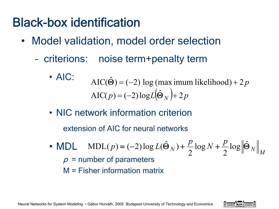
• Model validation, model order selection
– criterions: noise term+penalty term
• AIC:
• NIC network information criterion
extension of AIC for neural networks
• MDLp = number of parameters
M = Fisher information matrix
( ) pLp N 2ˆlog)2()(AIC +−= Θ
p2)likelihood imum(maxlog)2()ˆ(AIC +−=Θ
MNNpNpLp Θ++Θ−= ˆlog2
log2
)ˆ(log)2()(MDL
Neural Networks for System Modeling • Gábor Horváth, 2005 Budapest University of Technology and Economics
Black-box identification
• Model validation, model order selection
– cross validation
• testing the model on new data (from
the same problem)
• leave out one cross validation
• leave out k cross validation
Neural Networks for System Modeling • Gábor Horváth, 2005 Budapest University of Technology and Economics
Black-box identification
• Model validation, model order selection
– variance-bias trade-off
difference between the model and the real
system
• model class is not properly selected: bias
• actual parameters of the model are not
correct: variance
Neural Networks for System Modeling • Gábor Horváth, 2005 Budapest University of Technology and Economics
Black-box identification
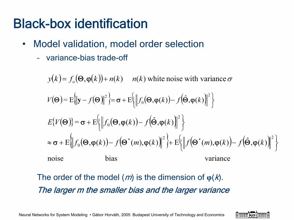
• Model validation, model order selection– variance-bias trade-off
The order of the model (m) is the dimension of φ(k).
The larger m the smaller bias and the larger variance
( ) ( )( ) σ ance with varinoise white)( )(, k nknkfky o += ϕΘ
( ) ( ) ( ) ( )⎭⎬⎫
⎩⎨⎧ −+=−
2
02 )(,ˆ)(,EE= kfkffV ϕΘϕΘσΘΘ y
( ) ( ) ( )( ) ( ) ( ) ( )
ance vari bias noise
)(,ˆ)(),(E)(),()(,E
)(,ˆ)(,E=
2*2*0
2
0
⎭⎬⎫
⎩⎨⎧ −+−+≈
⎭⎬⎫
⎩⎨⎧ −+
kfkmfkmfkf
kfkfVE
ϕΘϕΘϕΘϕΘσ
ϕΘϕΘσΘ
Neural Networks for System Modeling • Gábor Horváth, 2005 Budapest University of Technology and Economics
Black-box identification
• Model validation, model order selection– approaches
• A sequence of models are used with increasing m
Validation using cross validation or some criterion e.g. AIC, MDL, etc.
• A complex model structure is used with a lot of parameters (over-parametrized model)
Select important parameters
– regularization
– early stopping
– pruning
Neural Networks for System Modeling • Gábor Horváth, 2005 Budapest University of Technology and Economics
Neural modeling
• Neural networks are (general) nonlinear black-box structures with “interesting” properties– general architecture
– universal approximator
– non-sensitive to over-parametrization
– inherent regularization
Neural Networks for System Modeling • Gábor Horváth, 2005 Budapest University of Technology and Economics
Neural networks
• Why neural networks?– There are many other black-box modeling approaches:
e.g. polynomial regression.
– Difficulty: curse of dimensionality
– In high-dimensional (N) problem and using M-th order
polynomial the number of the independently adjustable
parameters will grow as NM.
– To get a trained neural network with good
generalization capability the dimension of the input
space has significant effect on the size of required
training data set.
Neural Networks for System Modeling • Gábor Horváth, 2005 Budapest University of Technology and Economics
Neural networks
• The advantages of neural approach
– Neural nets (MLP) use basis functions to
approximate nonlinear mappings, which
depend on the function to be approximated.
– This adaptive basis function set gives the
possibility to decrease the number of free
parameters in our general model structure.
Neural Networks for System Modeling • Gábor Horváth, 2005 Budapest University of Technology and Economics
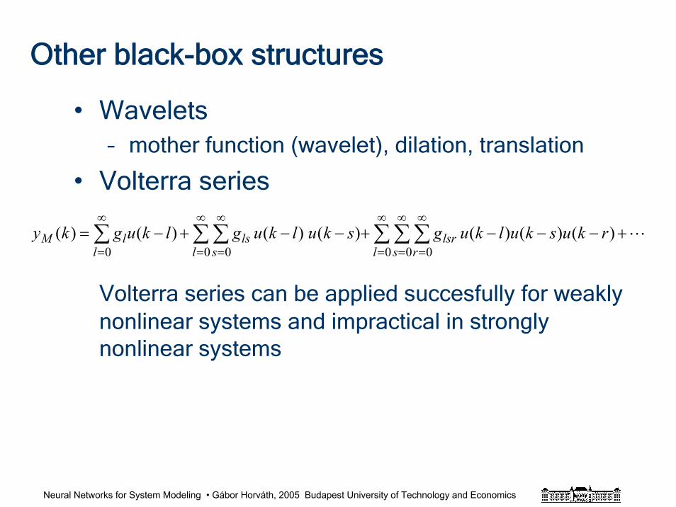
Other black-box structures
• Wavelets– mother function (wavelet), dilation, translation
• Volterra series
Volterra series can be applied succesfully for weakly nonlinear systems and impractical in strongly nonlinear systems
L+−−−+−−+−= ∑ ∑ ∑∑ ∑ ∑∞
=
∞
=
∞
=
∞
=
∞
=
∞
=)()()()()()()(
0 0 00 0 0rkuskulkugskulkuglkugky
l s rlsr
l l slslM
Neural Networks for System Modeling • Gábor Horváth, 2005 Budapest University of Technology and Economics
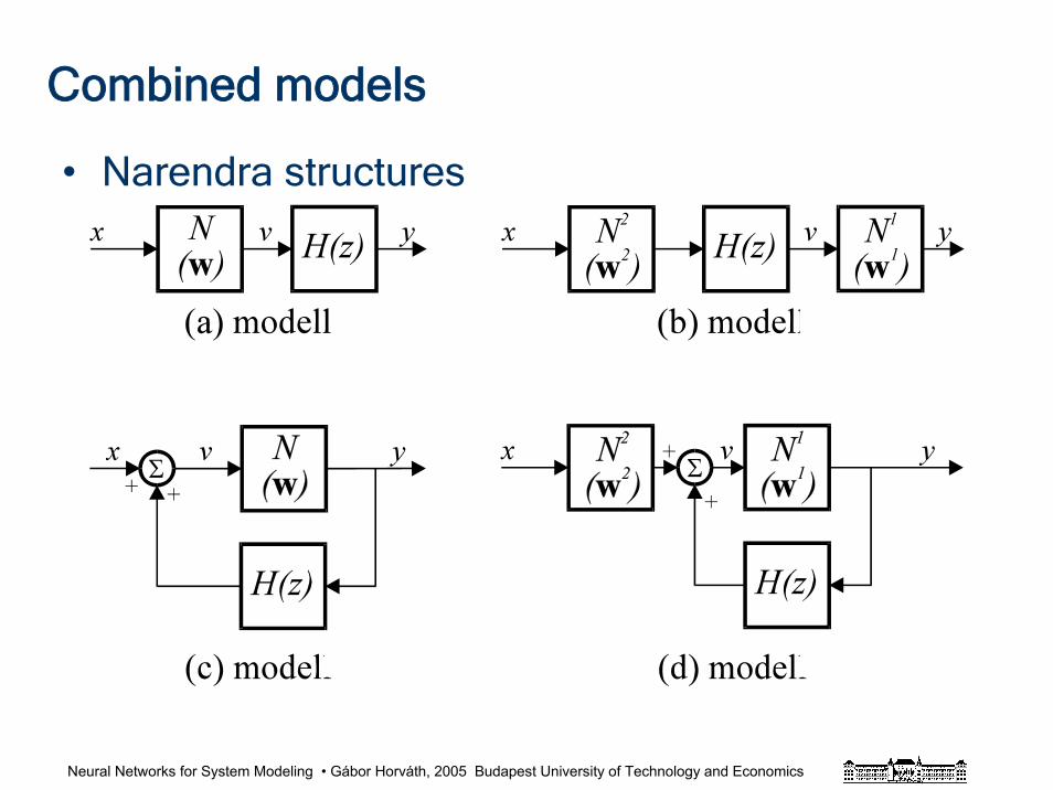
•Fuzzy models, fuzzy neural models
– general nonlinear modeling approach
•Wiener, Hammerstein, Wiener-Hammerstein
– dynamic linear system + static nonlinear
– static nonlinear + dynamic linear system
– dynamic linear system + static nonlinear + dynamic linear
•Narendra structures
– other combined linear dynamic and nonlinear static systems
Other black-box structures
Neural Networks for System Modeling • Gábor Horváth, 2005 Budapest University of Technology and Economics
Combined models
• Narendra structures
Neural Networks for System Modeling • Gábor Horváth, 2005 Budapest University of Technology and Economics
References and further readingsAkaike, H. “Information Theory and an Extension of the Maximum Likelihood Principle” Second Intnl. Symposium on Information Theory. Akadémiai Kiadó, Budapest, pp. 267-281. 1972.Akaike, H. “A New Look at the Statistical Model Identification” IEEE Trans. On Automatic Control, Vol. 19. No. 9. pp. 716-723. 1974.Haykin, S.: "Neural Networks. A Comprehensive Foundation" Prentice Hall, N. J.1999.
L. Ljung, ”System Identification - Theory for the User” Prentice-Hall, N.J. 2nd edition, 1999.
Narendra, K. S. and Pathasarathy, K. "Identification and Control of Dynamical Systems Using Neural Networks," IEEE Trans. Neural Networks, Vol. 1. 1990. pp. Noboru Murata, Shuji Yoshizawa and Shun-Ichi Amari “Network Information Criterion - Determining the Number of Hidden Units for an Artificial Neural Network Model” IEEE Trans. on Neural Networks, Vol. 5. No. 6. Pp. 865-871Pataki, B., Horváth, G., Strausz, Gy. and Talata, Zs. "Inverse Neural Modeling of a Linz-DonawitzSteel Converter" e & i Elektrotechnik und Informationstechnik, Vol. 117. No. 1. 2000. pp. 13-17.M.B. Priestley, “ Non-linear and Non-stationary Time Series Analysis” Academic Press, London, 1988.
Rissanen, J. “Stochastic Complexity in Statistical Inquiry”, Series in Computer Science”. Vol. 15 World Scientific, 1989.J. Sjöberg, Q. Zhang, L. Ljung, A. Benveniste, B. Delyon, P.-Y. Glorennec, H. Hjalmarsson, and A. Juditsky: "Non-linear Black-box Modeling in System Identification: a Unified Overview", Automatica, 31:1691-1724, 1995. A. S Weigend,. - N.A Gershenfeld "Forecasting the Future and Understanding the Past" Vol.15. Santa Fe Institute Studies in the Science of Complexity, Reading, MA. Addison-Wesley, 1994.
Neural Networks for System Modeling • Gábor Horváth, 2005 Budapest University of Technology and Economics
Neural networks
Neural Networks for System Modeling • Gábor Horváth, 2005 Budapest University of Technology and Economics
Outline• Introduction• Neural networks
– elementary neurons– classical neural structures– general approach – computational capabilities of NNs
• Learning (parameter estimation)– supervised learning– unsupervised learning– analytic learning
• Support vector machines– SVM architectures– statistical learning theory
• General questions of network design– generalization– model selection– model validation
Neural Networks for System Modeling • Gábor Horváth, 2005 Budapest University of Technology and Economics
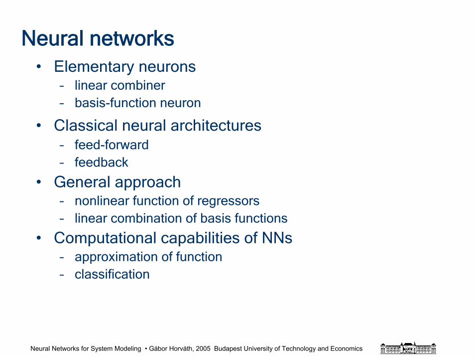
Neural networks• Elementary neurons
– linear combiner– basis-function neuron
• Classical neural architectures– feed-forward– feedback
• General approach– nonlinear function of regressors– linear combination of basis functions
• Computational capabilities of NNs– approximation of function– classification
Neural Networks for System Modeling • Gábor Horváth, 2005 Budapest University of Technology and Economics
Neural networks (a definition)
Neural networks are massively parallel distributed information processing systems, implemented in hardware or software form
made up of: a great number highly interconnected identical or similar simple processing units (processing elements, neurons) which are doing local processing, and are arranged in ordered topology,
have learning algorithm to acquire knowledge from their environment, using examples
have recall algorithm to use the learned knowledge
Neural Networks for System Modeling • Gábor Horváth, 2005 Budapest University of Technology and Economics
Neural networks (main features)
• Main features– complex nonlinear input-output mapping
– adaptivity, learning capability
– distributed architecture
– fault tolerance
– VLSI implementation
– neurobiological analogy
Neural Networks for System Modeling • Gábor Horváth, 2005 Budapest University of Technology and Economics
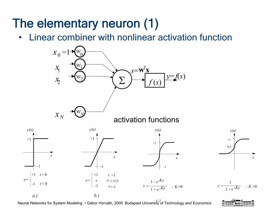
The elementary neuron (1)
=1
x1
x2
xN
0
y=f(s)f (s)
w0
s=wTxw1
w2
wN
x
Σ
• Linear combiner with nonlinear activation function
y= y=
-1 _
s
s
y(s) y(s)
s s
- 1 -1
+1 +1
a.) b.)
+1 >
s <
+1
-1
>1
-1 < s <1 _ _
s
s <-1
0
0
activation functions
y ________1
1 + -Ks ; K
y(s)
s
+1
d.)
y ________1 -
1 +
-Ks
-Ks ; K
y(s)
s
-1
+1
c.)
e= =
e e
0,5
>0>0
Neural Networks for System Modeling • Gábor Horváth, 2005 Budapest University of Technology and Economics
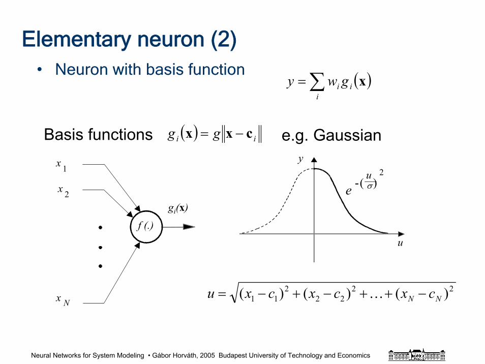
Elementary neuron (2)• Neuron with basis function
gi(x)
f (.)
x
x
1
2
x N
u
y
e -( )u 2σ
( )x∑=i
ii gwy
( ) ii gg cxx −=Basis functions e.g. Gaussian
2222
211 )()()( NN cxcxcxu −++−+−= K
Neural Networks for System Modeling • Gábor Horváth, 2005 Budapest University of Technology and Economics
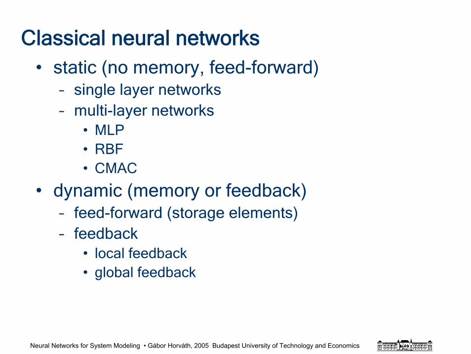
Classical neural networks• static (no memory, feed-forward)
– single layer networks– multi-layer networks
• MLP• RBF• CMAC
• dynamic (memory or feedback)– feed-forward (storage elements)– feedback
• local feedback• global feedback
Neural Networks for System Modeling • Gábor Horváth, 2005 Budapest University of Technology and Economics
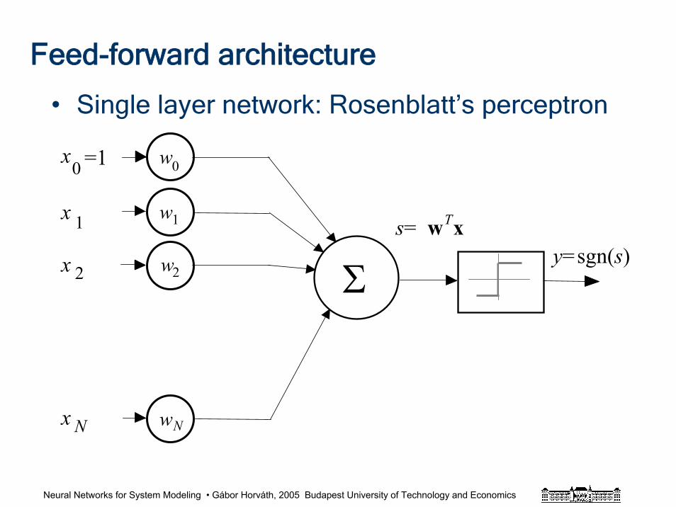
Feed-forward architecture
• Single layer network: Rosenblatt’s perceptron
=1
x 1
x 2
x N
0
y=sgn(s)
w0
s= wTxw1
w2
wN
x
Σ
Neural Networks for System Modeling • Gábor Horváth, 2005 Budapest University of Technology and Economics
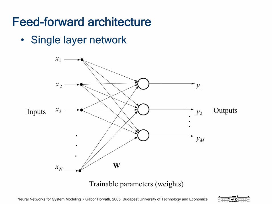
Feed-forward architecture
• Single layer network
OutputsInputs
x
x
x
x
y
y
y
W
Trainable parameters (weights)
N
1
12
23
M
Neural Networks for System Modeling • Gábor Horváth, 2005 Budapest University of Technology and Economics
Feed-forward architecture
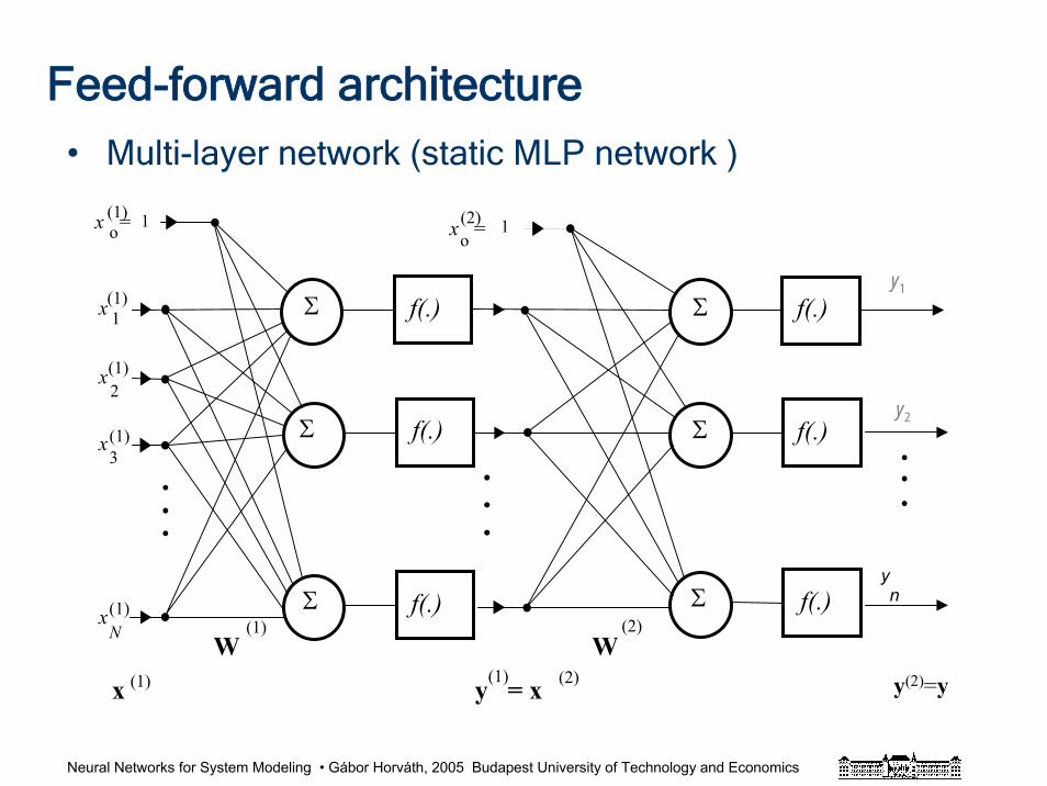
y(2)=y
yn
y = xx (1) (2)
x =oo(2)
Σ
Σ
Σ
Σ
Σ
Σ
W(2)(1)
(1)W
1 1x =
x
x
x
x
1
2
3
N
(1)
(1)
(1)
(1)
(1) f(.) f(.)
f(.)
f(.) f(.)
f(.)
y1
y2
• Multi-layer network (static MLP network )
Neural Networks for System Modeling • Gábor Horváth, 2005 Budapest University of Technology and Economics
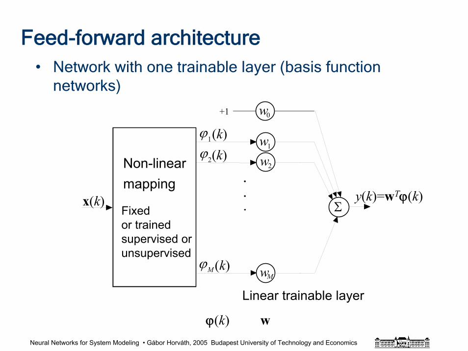
Feed-forward architecture• Network with one trainable layer (basis function
networks)
(k)(k)
(k)
1
2
M
x(k) y(k)=wTϕ(k)mapping
X
Σ
Linear trainable layer
w
1
+1
w
w
w
0
2
wM
1
Non-linear
ϕ
ϕ ϕ
Fixedor trainedsupervised or unsupervised
ϕ(k) w
Neural Networks for System Modeling • Gábor Horváth, 2005 Budapest University of Technology and Economics
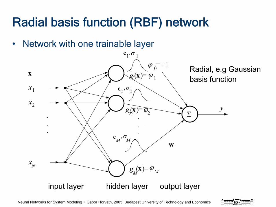
Radial basis function (RBF) network
• Network with one trainable layerσ
g =
x
x
1
2
N
y
+1
w
c
c
c
Σ
1,
,σ
,σ
2
M M
input layer hidden layer output layer
x
ϕ =0
g =
g =
2
1
1 1
2 2
M M
( )
( )
( )
x
x
x
x ϕ
ϕ
ϕ
Radial, e.g Gaussian basis function
Neural Networks for System Modeling • Gábor Horváth, 2005 Budapest University of Technology and Economics
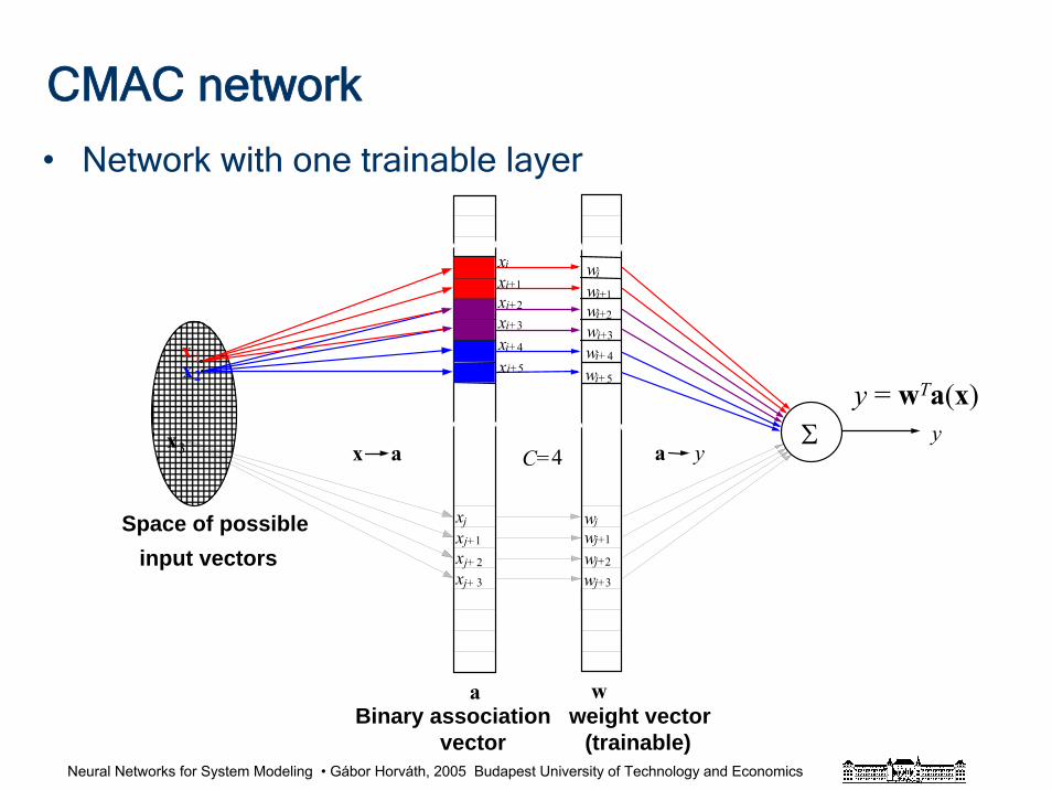
CMAC network
• Network with one trainable layer
Σ
Space of possibleinput vectors
xx
i+
i+3
x a a y
y
wwwww
i
i+
i+
i+
2
1
3
C=4
waBinary association weight vector
vector (trainable)
x1
2
i+
i+
4
5x
x
2
3
xx
xx
j+
j+
1
2
3
j j
j+
w
wwww
j+
j+
j+
1
3
2
xi
x
x
x
i+1
i+
i+
4
5
y = wTa(x)
Neural Networks for System Modeling • Gábor Horváth, 2005 Budapest University of Technology and Economics
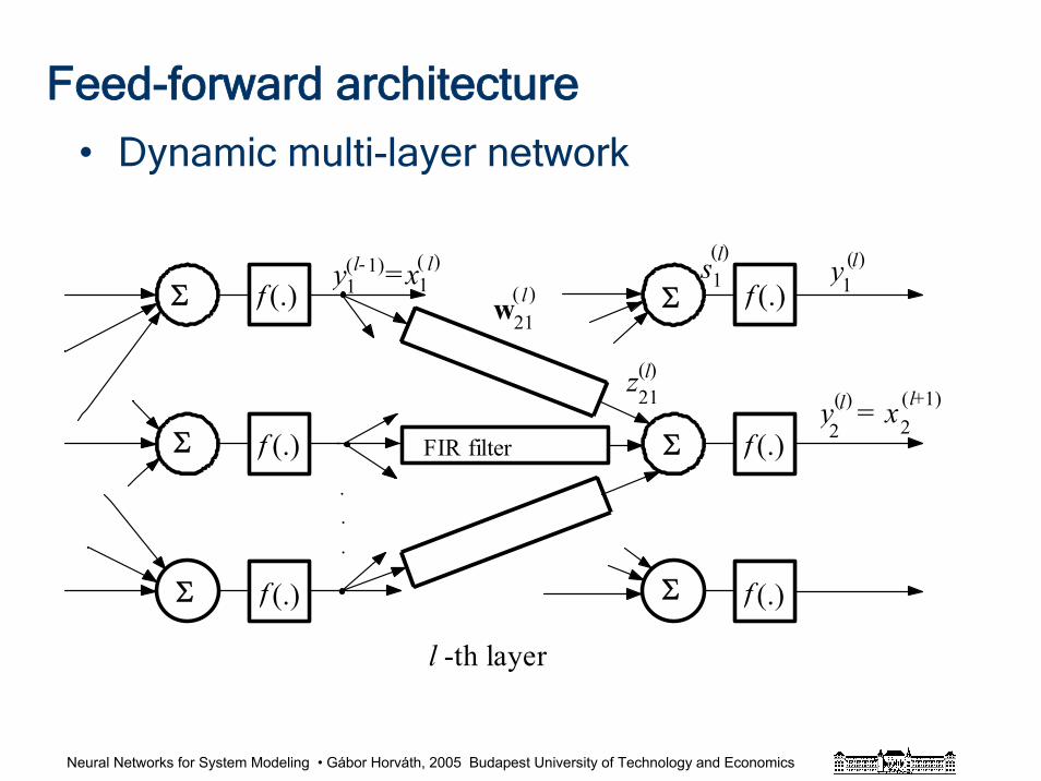
Feed-forward architecture
• Dynamic multi-layer network
( +1)
s
z
y =x
FIR filter
(.) (.)
(.)
(.)
(.)
(.)
Σ
Σ
Σ Σ
Σ
Σ
-th layer
( )
( )
1 y
y = x
1
( )
( )
2 2
21
l
.
.
.
l l
l l l
f f
f
f f
f
1 1 l- l ( 1) ( )
w l ( )
21
Neural Networks for System Modeling • Gábor Horváth, 2005 Budapest University of Technology and Economics
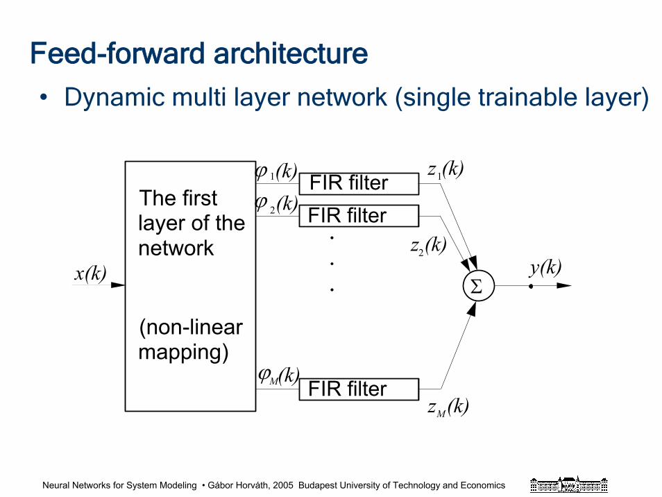
Feed-forward architecture
• Dynamic multi layer network (single trainable layer)
FIR filterFIR filter
FIR filter
Σ
(k) (k)
(k)
1
2
M
x(k)
z (k)
z (k)
1
M
y(k)z (k)2
The firstlayer of thenetwork
(non-linearmapping)
ϕ
ϕϕ
Neural Networks for System Modeling • Gábor Horváth, 2005 Budapest University of Technology and Economics
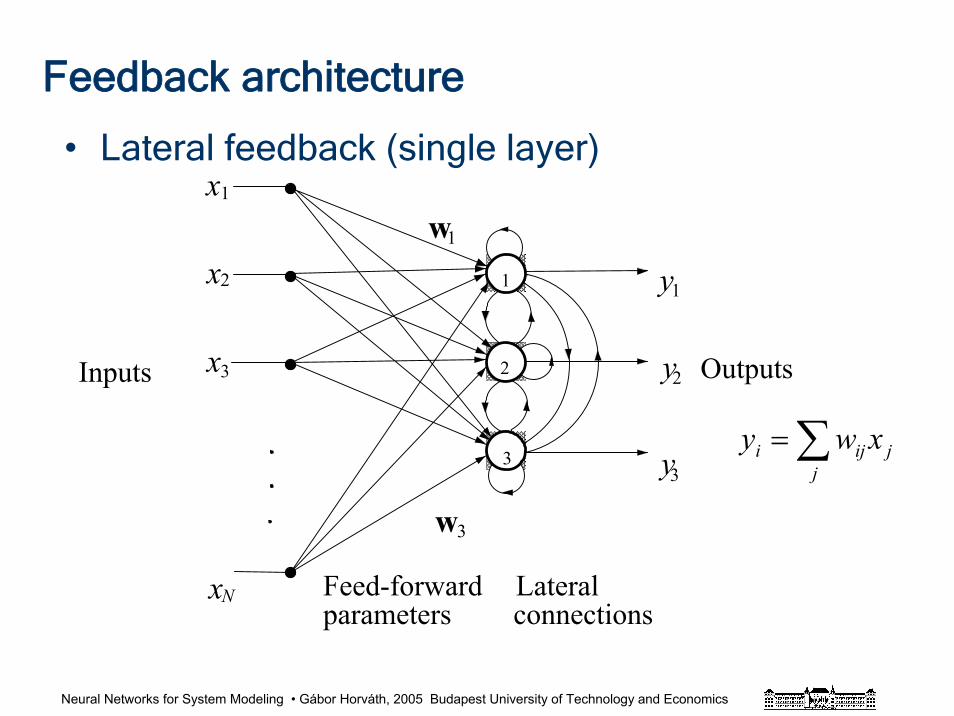
Feedback architecture
• Lateral feedback (single layer)
OutputsInputs
x
x
x
x Feed-forwardparameters
y
y
y
Lateralconnections
3
N
2
2
1
3
w
w
1
1
3
1
2
3 ∑=j
jiji xwy
Neural Networks for System Modeling • Gábor Horváth, 2005 Budapest University of Technology and Economics
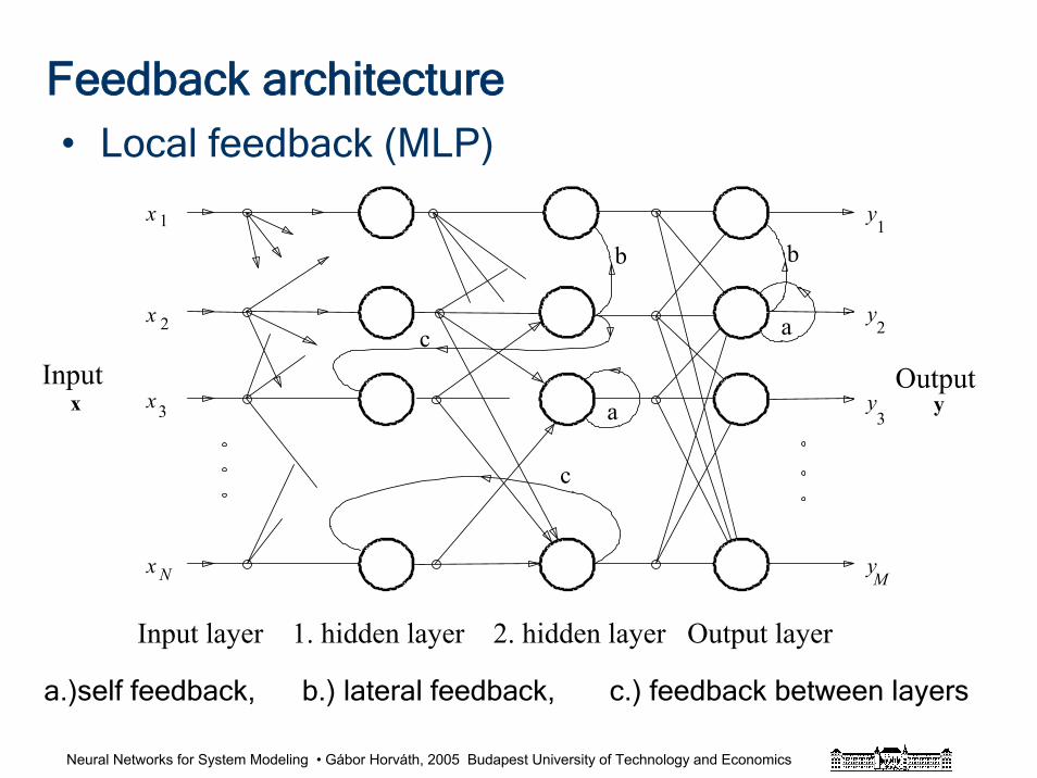
Feedback architecture
Input layer 1. hidden layer 2. hidden layer Output layer
a
a
b b
c
c
x
x
x
x
x
yInput Output
y
y
y
y
1 1
2 2
3 3
N M
a.)self feedback, b.) lateral feedback, c.) feedback between layers
• Local feedback (MLP)
Neural Networks for System Modeling • Gábor Horváth, 2005 Budapest University of Technology and Economics
Feedback architecture
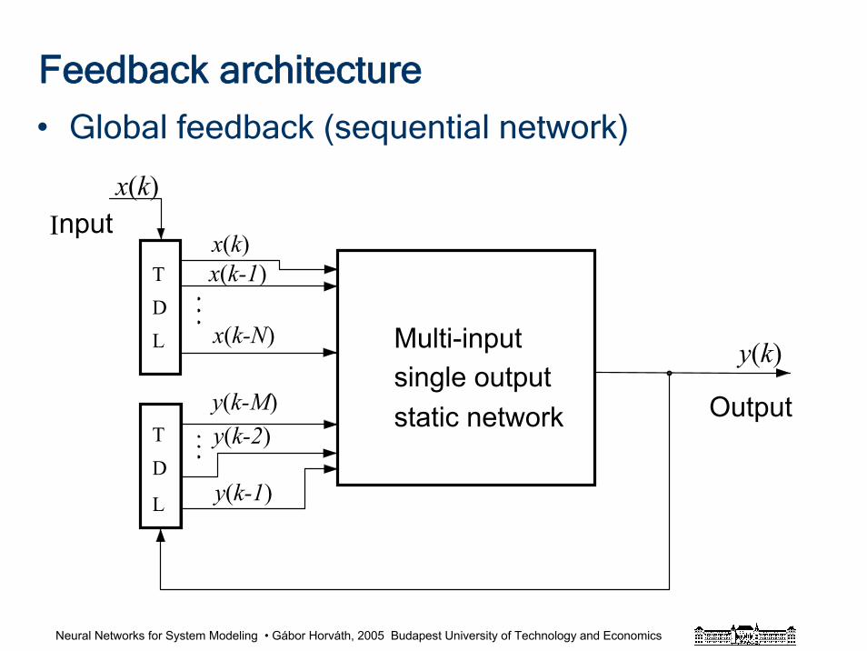
• Global feedback (sequential network)
Multi-inputsingle output
TDL
TD
L
Input
Outputstatic network
x(k-1)
x(k-N)
x(k)
x(k)
y(k)
y(k-M)y(k-2)
y(k-1)
Neural Networks for System Modeling • Gábor Horváth, 2005 Budapest University of Technology and Economics
Feedback architecture
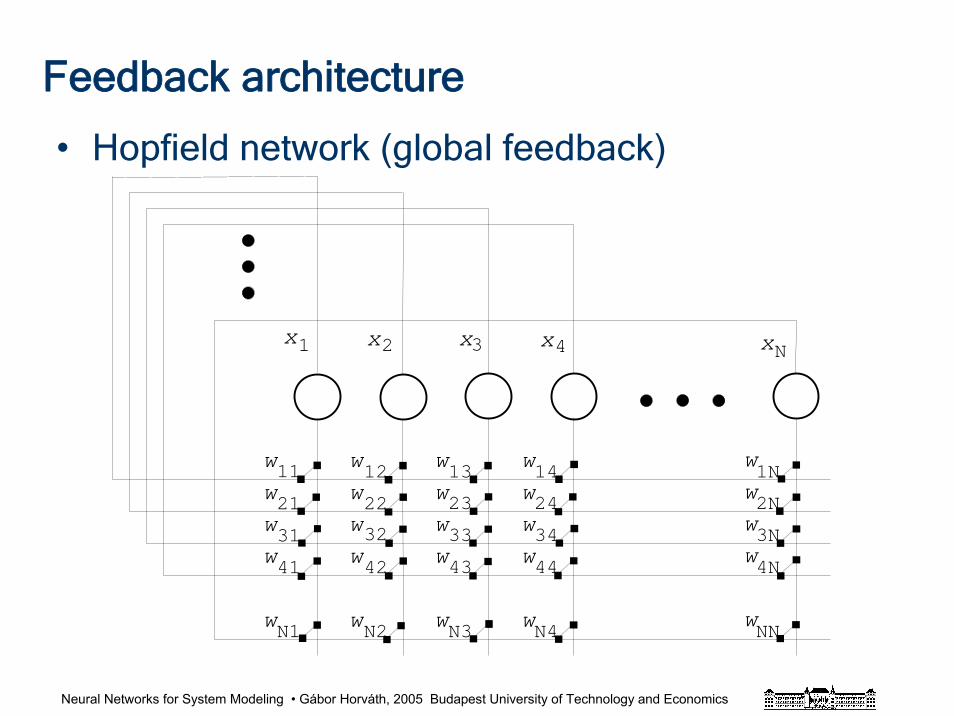
• Hopfield network (global feedback)
N1
wwww
w
13 14 1N
2N
3N
24
34
44 4N
N4 NN
23
33
12
22
32
42 43
11
21
31
41
N2 N3
x x x x x1 2 3 4 N
wwww
w
wwww
w
wwww
w
wwww
w
Neural Networks for System Modeling • Gábor Horváth, 2005 Budapest University of Technology and Economics
Basic neural network architectures
• Genaral approach– Regressors
• current inputs (static networks)
• current inputs and past outputs (dynamic networks)
• past inputs and past outputs (dynamic networks)
– Basis functions• non-linear-in-the-parameter network
• linear-in-the-parameter networks
Neural Networks for System Modeling • Gábor Horváth, 2005 Budapest University of Technology and Economics
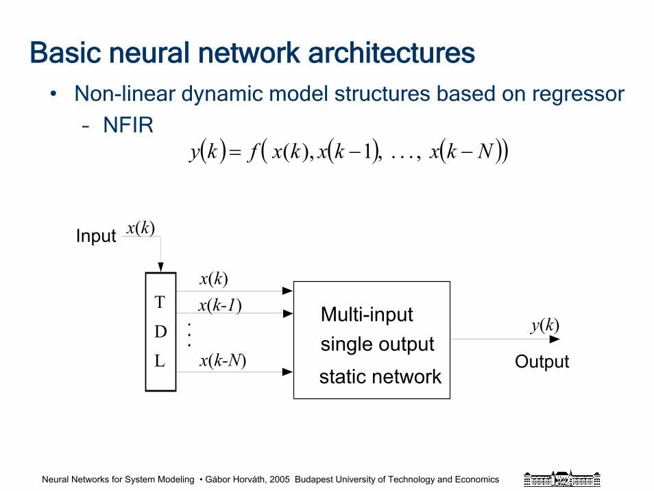
Basic neural network architectures• Non-linear dynamic model structures based on regressor
– NFIR
Multi-inputsingle output
TDL
Input
Outputstatic network
x(k-1)
x(k-N)
x(k)
x(k)
y(k)
( ) ( ) ( )( )Nkxkxkxfky −−= ,...,1),(
Neural Networks for System Modeling • Gábor Horváth, 2005 Budapest University of Technology and Economics
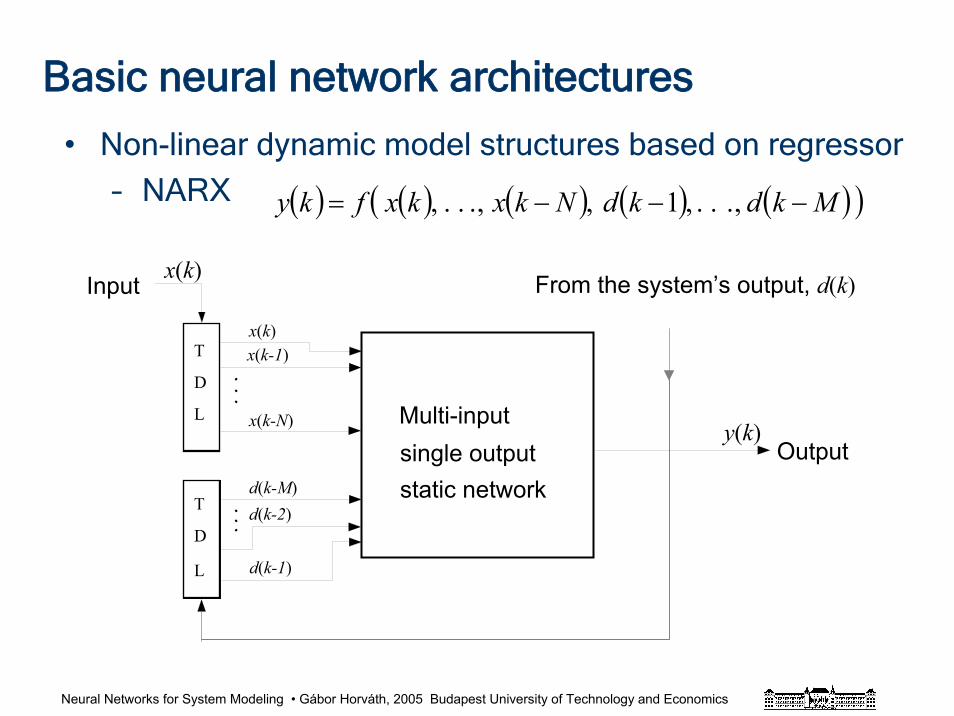
Basic neural network architectures
• Non-linear dynamic model structures based on regressor
– NARX
From the system’s output, d(k)
Multi-inputsingle output
T
D
L
T
D
L
Input
Outputstatic network
x(k-1)
x(k-N)
x(k)
x(k)
y(k)
d(k-M)d(k-2)
d(k-1)
( ) ( ) ( ) ( ) ( )( )MkdkdNkxkxfky −−−= ,...,1,,...,
Neural Networks for System Modeling • Gábor Horváth, 2005 Budapest University of Technology and Economics
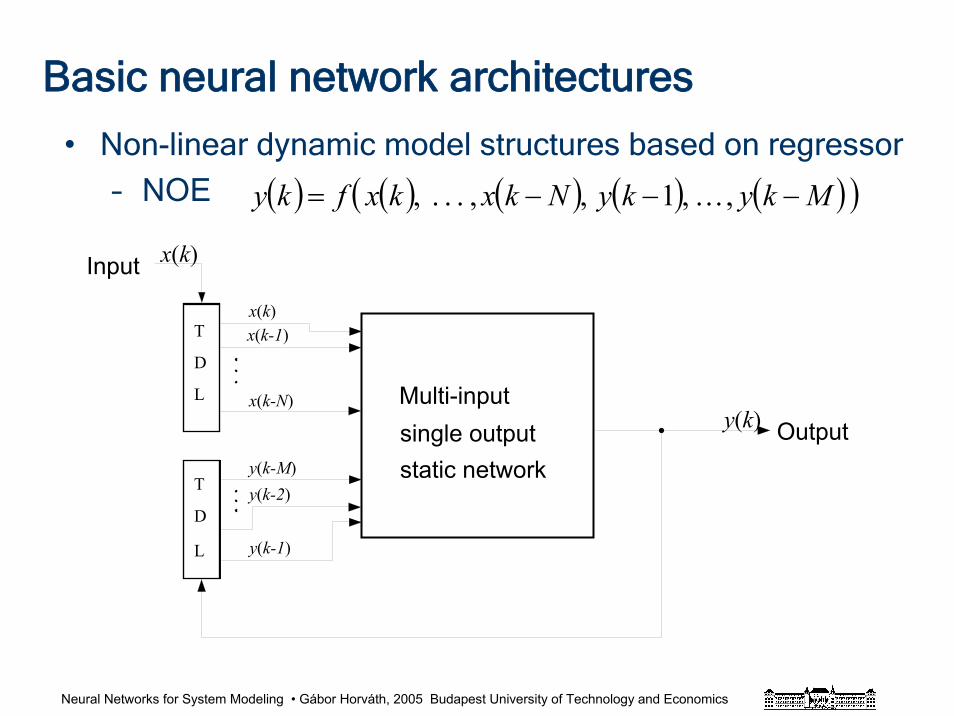
Basic neural network architectures
• Non-linear dynamic model structures based on regressor
– NOE
Multi-inputsingle output
T
D
L
T
D
L
Input
Outputstatic network
x(k-1)
x(k-N)
x(k)
x(k)
y(k)
y(k-M)y(k-2)
y(k-1)
( ) ( ) ( ) ( ) ( )( )MkykyNkxkxfky −−−= ,...,1,,...,
Neural Networks for System Modeling • Gábor Horváth, 2005 Budapest University of Technology and Economics
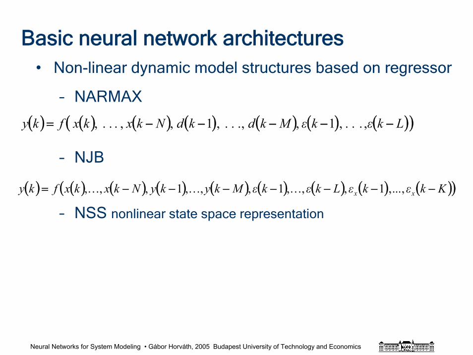
Basic neural network architectures• Non-linear dynamic model structures based on regressor
– NARMAX
– NJB
– NSS nonlinear state space representation
( ) ( ) ( ) ( ) ( ) ( ) ( )( )LkεkεMkdkdNkxkxfky −−−−−= ,...,1,,...,1,,...,
( ) ( ) ( ) ( ) ( ) ( ) ( ) ( ) ( )( )KkεkεLkεkεMkykyNkxkxfky xx −−−−−−−= ,...,1,,...,1,,...,1,,...,
Neural Networks for System Modeling • Gábor Horváth, 2005 Budapest University of Technology and Economics
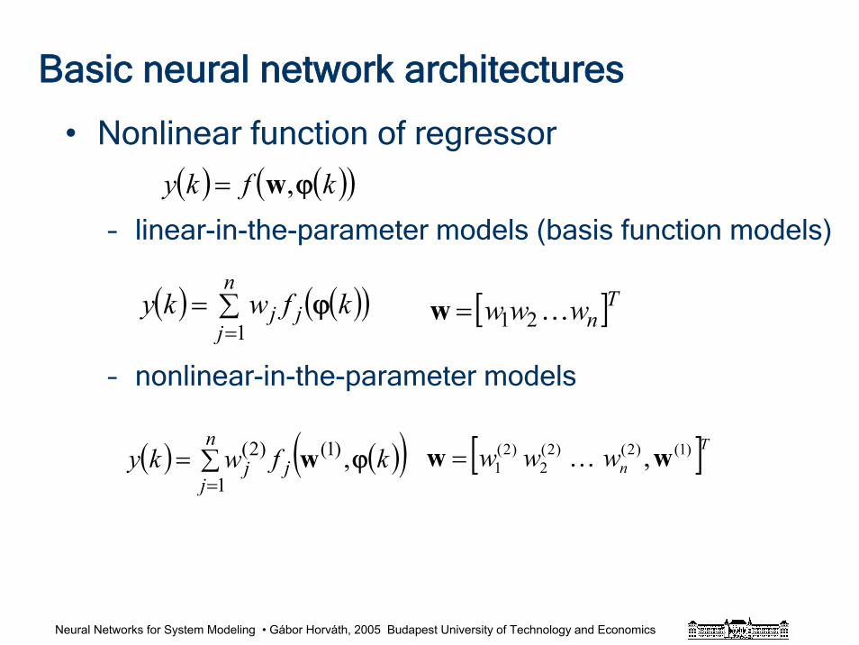
Basic neural network architectures
• Nonlinear function of regressor
– linear-in-the-parameter models (basis function models)
– nonlinear-in-the-parameter models
( ) ( )( )kfky ϕ,w=
( ) ( )( )kfwky jn
jj ϕ,)1(
1
)2( w∑==
[ ]Tnwww )1()2()2(2
)2(1 ,ww K=
( ) ( )( )kfwky jn
jj ϕ∑=
=1[ ]Tnwww K21=w
Neural Networks for System Modeling • Gábor Horváth, 2005 Budapest University of Technology and Economics
Basic neural network architectures
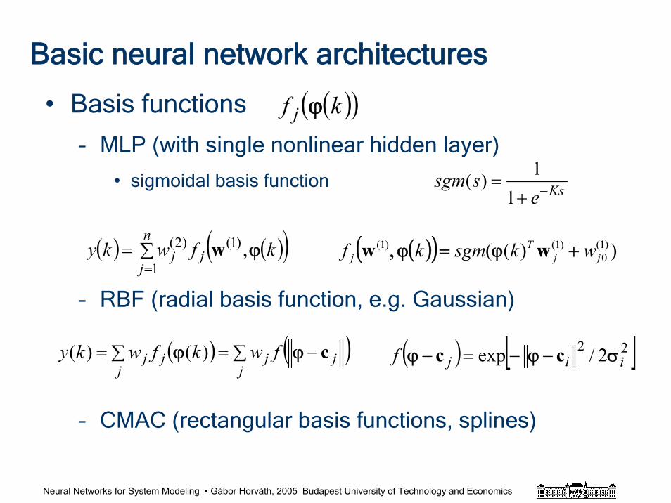
• Basis functions
– MLP (with single nonlinear hidden layer)
• sigmoidal basis function
– RBF (radial basis function, e.g. Gaussian)
– CMAC (rectangular basis functions, splines)
( )( )kf j ϕ
( )( ) ))(( )1(0
)1()1(jj
Tj wksgmkf +ϕ=ϕ, ww
Ksessgm −+
=1
1)(
( ) ( )( )kfwky jn
jj ϕ,)1(
1
)2( w∑==
( ) ( )∑ −=∑=j
jjj
jj fwkfwky cϕϕ )()( ( ) [ ]22 2/exp iijf σϕϕ cc −−=−
Neural Networks for System Modeling • Gábor Horváth, 2005 Budapest University of Technology and Economics
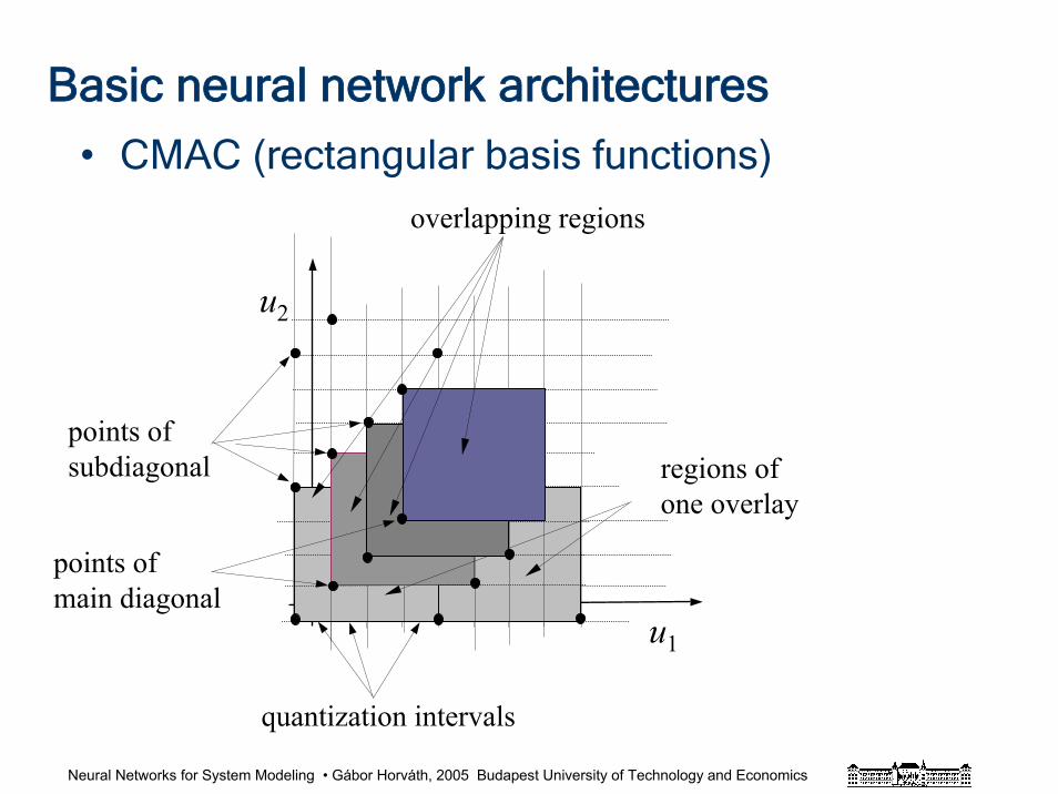
• CMAC (rectangular basis functions)
Basic neural network architectures
quantization intervals
u1
u2
overlapping regions
regions ofone overlay
points of main diagonal
points ofsubdiagonal
Neural Networks for System Modeling • Gábor Horváth, 2005 Budapest University of Technology and Economics
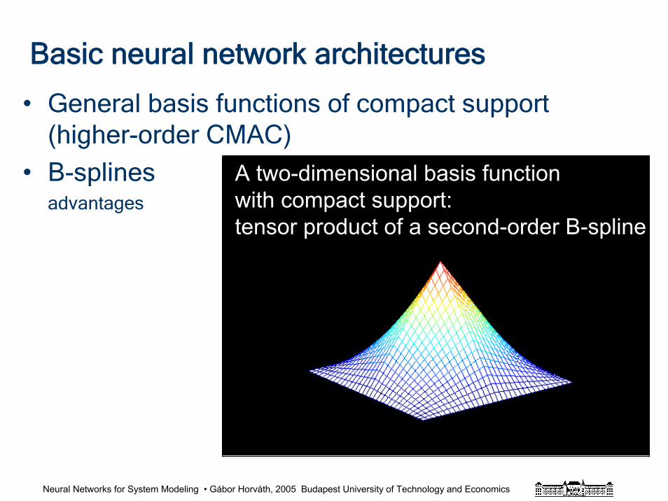
• General basis functions of compact support (higher-order CMAC)
• B-splinesadvantages
Basic neural network architectures
A two-dimensional basis function with compact support: tensor product of a second-order B-spline
Neural Networks for System Modeling • Gábor Horváth, 2005 Budapest University of Technology and Economics
Capability of networks
Neural Networks for System Modeling • Gábor Horváth, 2005 Budapest University of Technology and Economics
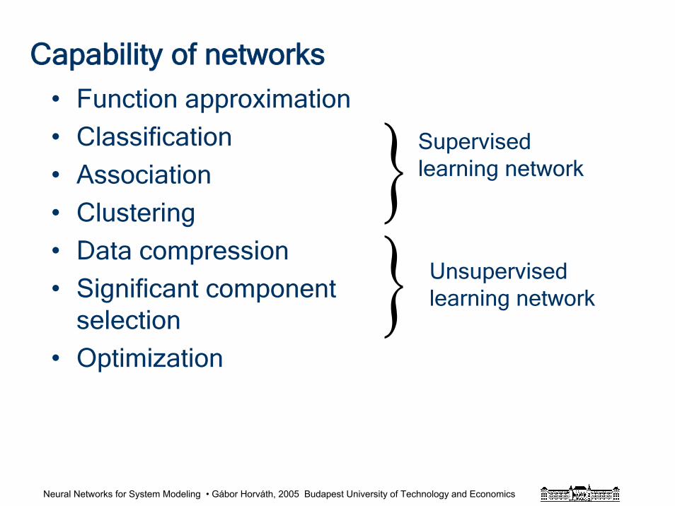
Capability of networks
• Function approximation
• Classification
• Association
• Clustering
• Data compression
• Significant component selection
• Optimization
Supervised learning network
Unsupervised learning network
Neural Networks for System Modeling • Gábor Horváth, 2005 Budapest University of Technology and Economics
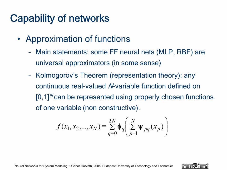
Capability of networks
• Approximation of functions– Main statements: some FF neural nets (MLP, RBF) are
universal approximators (in some sense)
– Kolmogorov’s Theorem (representation theory): any
continuous real-valued N-variable function defined on
[0,1]N can be represented using properly chosen functions
of one variable (non constructive).
)(=),...,,(1
2
0=21 ⎟⎟
⎠
⎞⎜⎜⎝
⎛∑∑=
N
pppq
N
qqN xxxxf ψφ
Neural Networks for System Modeling • Gábor Horváth, 2005 Budapest University of Technology and Economics
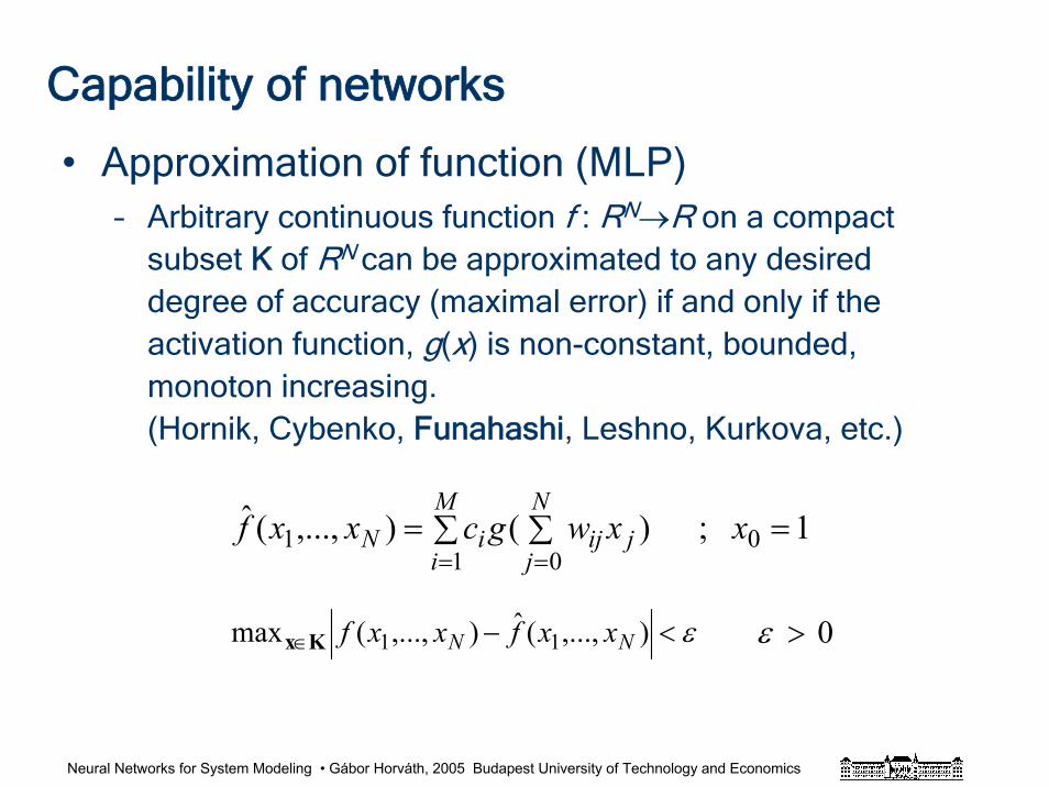
Capability of networks
• Approximation of function (MLP)– Arbitrary continuous function f : RN→R on a compact
subset K of RN can be approximated to any desired degree of accuracy (maximal error) if and only if the activation function, g(x) is non-constant, bounded, monoton increasing. (Hornik, Cybenko, Funahashi, Leshno, Kurkova, etc.)
∑ ∑ === =
M
i
N
jjijiN xxwgcxxf
1 001 1 ; )(),...,(ˆ
ε<−∈ ),...,(ˆ),...,(max 11 NN xxfxxfKx 0>ε
Neural Networks for System Modeling • Gábor Horváth, 2005 Budapest University of Technology and Economics
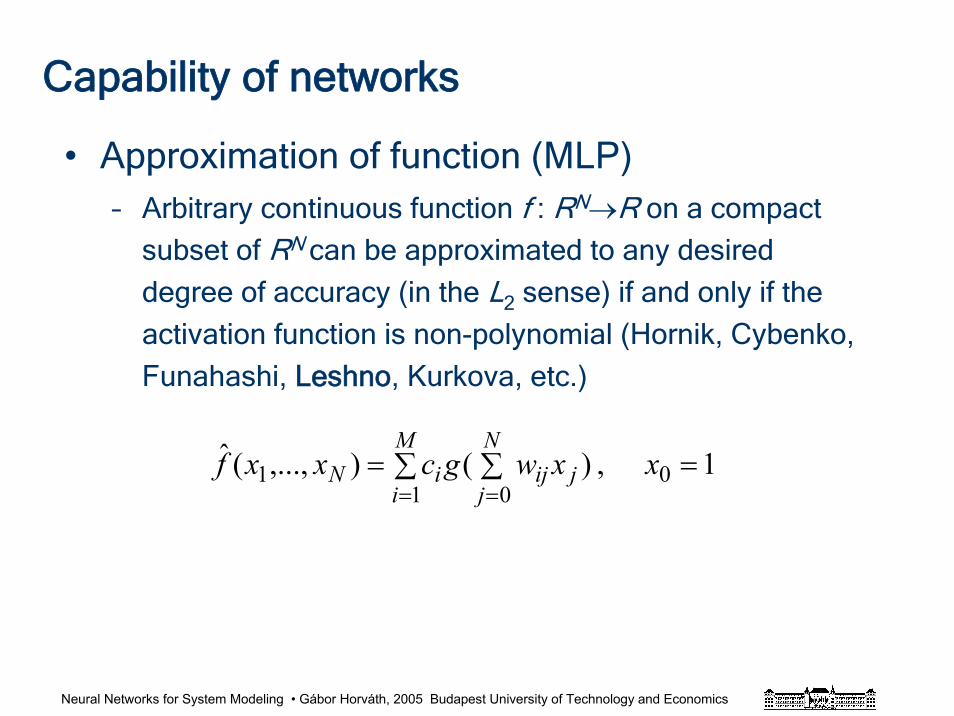
Capability of networks
• Approximation of function (MLP)– Arbitrary continuous function f : RN→R on a compact
subset of RN can be approximated to any desired
degree of accuracy (in the L2 sense) if and only if the
activation function is non-polynomial (Hornik, Cybenko,
Funahashi, Leshno, Kurkova, etc.)
∑ ∑ === =
M
i
N
jjijiN xxwgcxxf
1 001 1 , )(),...,(ˆ
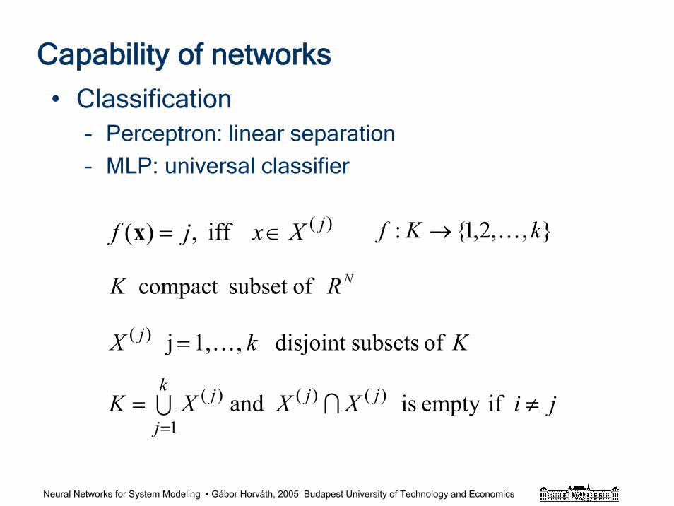
Neural Networks for System Modeling • Gábor Horváth, 2005 Budapest University of Technology and Economics
• Classification– Perceptron: linear separation
– MLP: universal classifier
Capability of networks
)( iff,)( jXxjf ∈=x ,,2,1: kKf K→
NRK ofsubset compact
jiXXXK
KkX
jjjk
j
j
≠=
=
= ifempty is and
of subsetsdisjoint ,1,j
)()()(
1
)(
IU
K
Neural Networks for System Modeling • Gábor Horváth, 2005 Budapest University of Technology and Economics
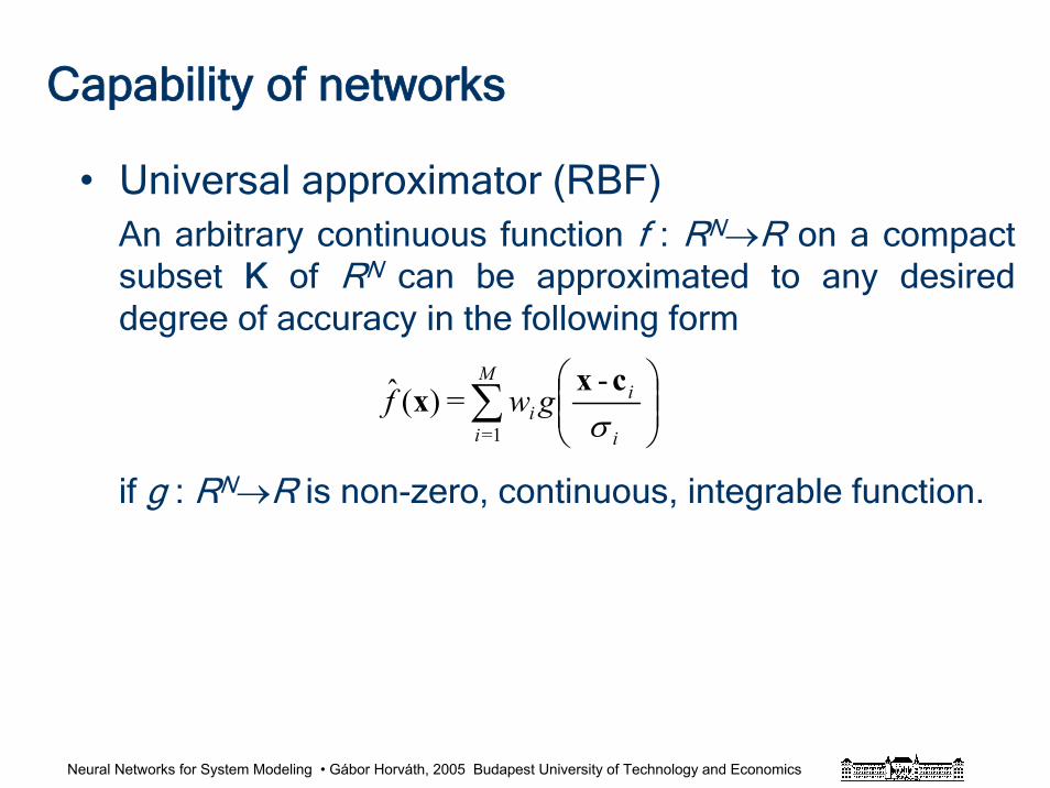
Capability of networks
• Universal approximator (RBF)An arbitrary continuous function f : RN→R on a compact subset K of RN can be approximated to any desired degree of accuracy in the following form
if g : RN→R is non-zero, continuous, integrable function.
-
= )(ˆ1=
∑ ⎟⎟⎠
⎞⎜⎜⎝
⎛M
i i
ii gwf
σcx
x
Neural Networks for System Modeling • Gábor Horváth, 2005 Budapest University of Technology and Economics
Computational capability of the CMAC
• The approximation capability of the Albus binary CMAC
• Single-dimensional (univariate) case
• Multi-dimensional (multivariate) case
Neural Networks for System Modeling • Gábor Horváth, 2005 Budapest University of Technology and Economics
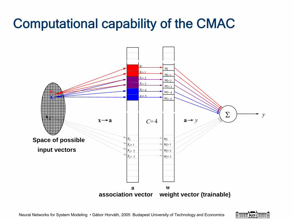
Computational capability of the CMAC
Σ
Space of possibleinput vectors
xx
i+
i+3
x a a y
y
wwwww
i
i+
i+
i+
2
1
3
C=4
waassociation vector weight vector (trainable)
x1
2
i+
i+
4
5x
x
2
3
xx
xx
j+
j+
1
2
3
j j
j+
w
wwww
j+
j+
j+
1
3
2
xi
x
x
x
i+1
i+
i+
4
5
Neural Networks for System Modeling • Gábor Horváth, 2005 Budapest University of Technology and Economics
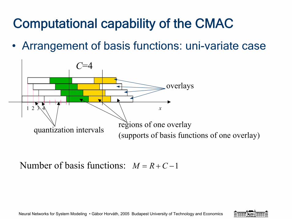
1 2 3 4 x
C=4
quantization intervalsregions of one overlay(supports of basis functions of one overlay)
overlays
Computational capability of the CMAC
• Arrangement of basis functions: uni-variate case
Number of basis functions: 1−+= CRM
Neural Networks for System Modeling • Gábor Horváth, 2005 Budapest University of Technology and Economics
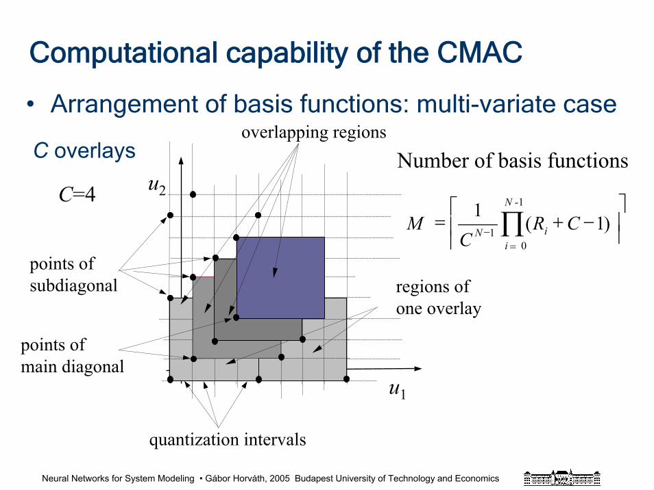
Computational capability of the CMAC
• Arrangement of basis functions: multi-variate case
quantization intervals
u1
u2
overlapping regions
regions ofone overlay
points of main diagonal
points ofsubdiagonal
Number of basis functions
⎥⎥
⎤)1(
1
01⎢
⎢
⎡−+= ∏
=−
N -1
iiN CR
CM
C overlays
C=4
Neural Networks for System Modeling • Gábor Horváth, 2005 Budapest University of Technology and Economics
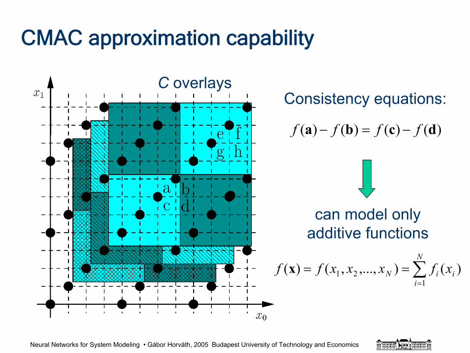
CMAC approximation capability
Basis functions
C overlaysConsistency equations:
)()()()( dcba ffff −=−
can model only additive functions
∑=
==N
iiiN xfxxxff
121 )(),...,,()(x
Neural Networks for System Modeling • Gábor Horváth, 2005 Budapest University of Technology and Economics
CMAC modeling capability
One-dimensional case: can learn any training data set exactly
Multi-dimensional case: can learn any training data set from the additive function set (consistency equations)
Neural Networks for System Modeling • Gábor Horváth, 2005 Budapest University of Technology and Economics
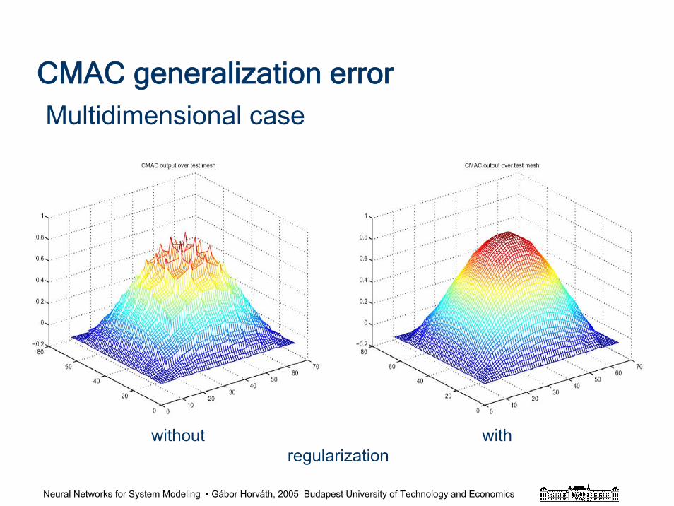
CMAC generalization capability
Important parameters:
C generalization parameterdtrain distance between adjacent training data
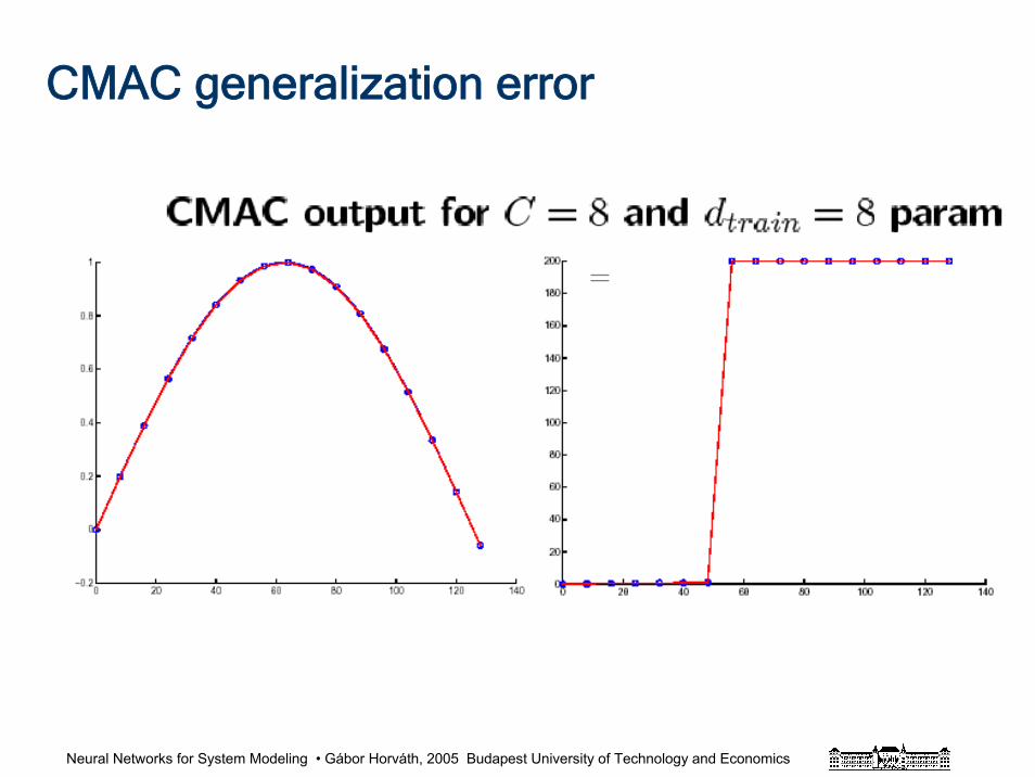
Interesting behaviorC=l*dtrain : linear interpolation between the
training points
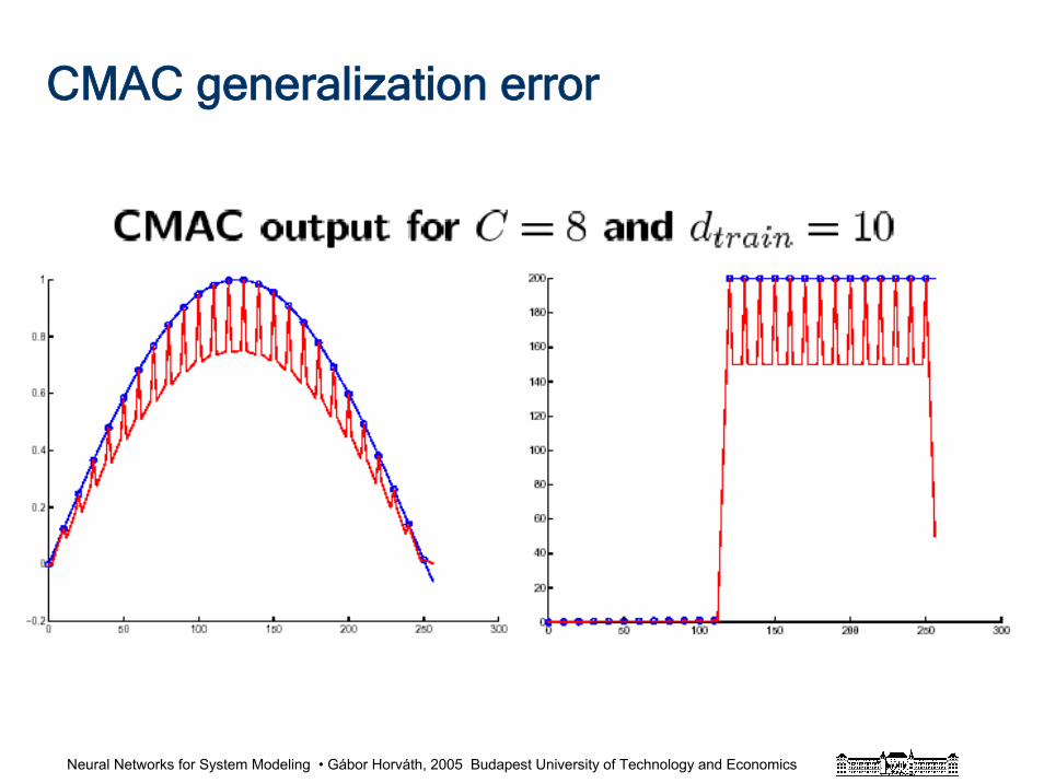
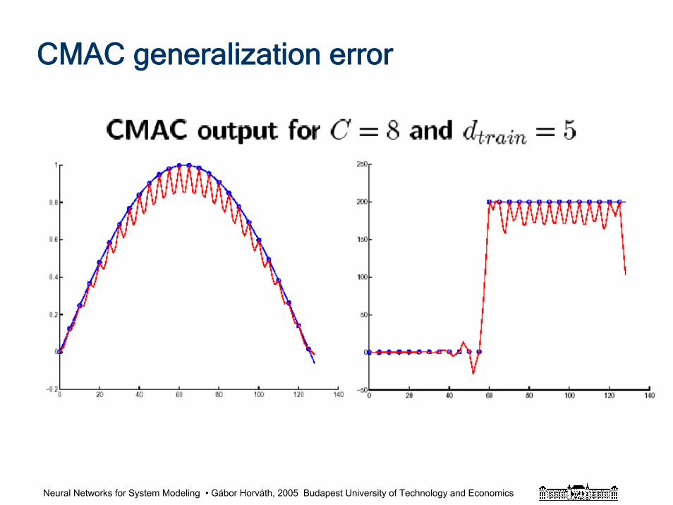
C≠l*dtrain : significant generalization error non-smooth output
Neural Networks for System Modeling • Gábor Horváth, 2005 Budapest University of Technology and Economics
CMAC generalization error
=
Neural Networks for System Modeling • Gábor Horváth, 2005 Budapest University of Technology and Economics
CMAC generalization error
Neural Networks for System Modeling • Gábor Horváth, 2005 Budapest University of Technology and Economics
CMAC generalization error
Neural Networks for System Modeling • Gábor Horváth, 2005 Budapest University of Technology and Economics
Multidimensional caseCMAC generalization error
without withregularization

Neural Networks for System Modeling • Gábor Horváth, 2005 Budapest University of Technology and Economics
CMAC generalization error univariate case (max)
1 2 3 4 5 6 7 80
0.02
0.04
0.06
0.08
0.1
0.12
0.14
0.16
0.18
0.2
C/dtrain
Abs. valueof max. rel. error
h
Neural Networks for System Modeling • Gábor Horváth, 2005 Budapest University of Technology and Economics
Application of networks (based on the capability)• Regression: function approximation
– modeling of static and dynamic systems, signal modeling, system identification
– filtering, control, etc.
• Pattern association– association
• autoassociation (similar input and output)
(dimension reduction, data compression)
• Heteroassociation (different input and output)
• Pattern recognition, clustering – classification
Neural Networks for System Modeling • Gábor Horváth, 2005 Budapest University of Technology and Economics
Application of networks (based on the capability)
• Optimization– optimization
• Data compression, dimension reduction– principal component analysis (PCA), linear
networks
– nonlinear PCA, non-linear networks
– signal separation, BSS, independent component analysis (ICA).
Neural Networks for System Modeling • Gábor Horváth, 2005 Budapest University of Technology and Economics
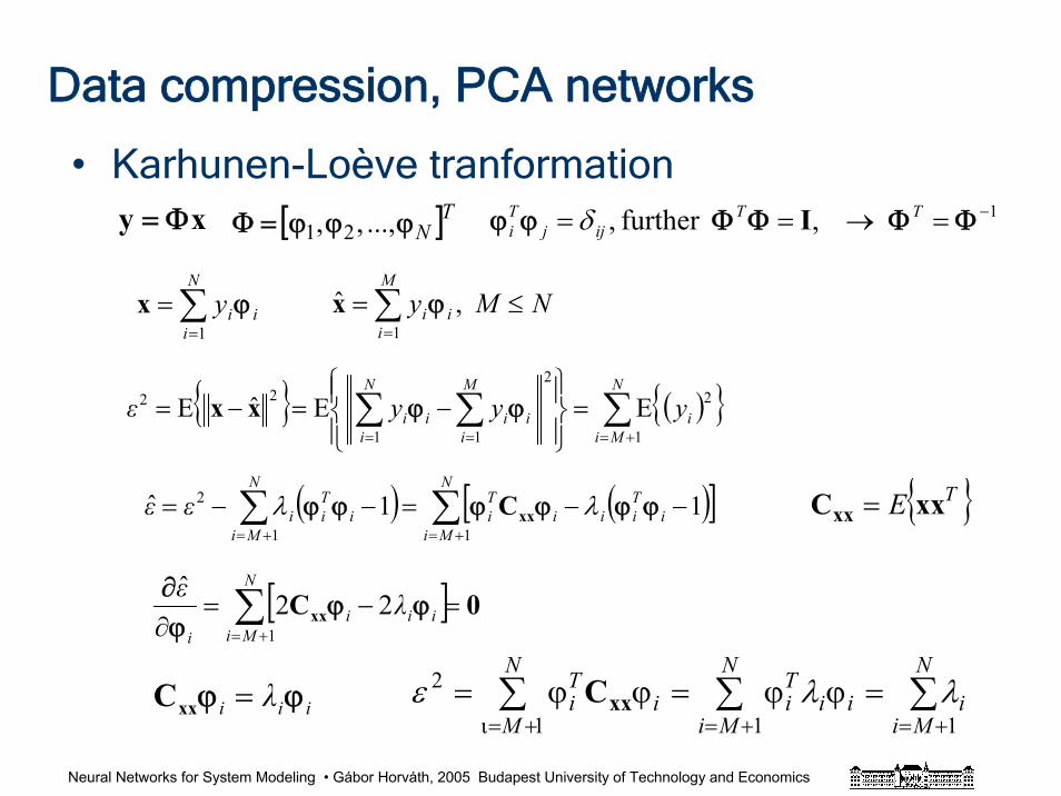
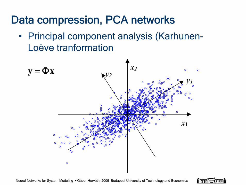
Data compression, PCA networks
• Karhunen-Loève tranformationxy Φ= [ ]TNϕϕϕ=Φ ..., ,, 21
1 ,further , −=→== ΦΦΦΦϕϕ TTijj
Ti Iδ
∑=
=N
iiiy
1ϕx NMy
M
iii ≤= ∑
=
,ˆ1
ϕx
( ) ∑∑ ∑+== =
=⎪⎭
⎪⎬⎫
⎪⎩
⎪⎨⎧
−=−=N
Mii
N
i
M
iiiii yyyε
1
22
1 1
22 EEˆE ϕϕxx
( ) ( )[ ]∑∑+=+=
−−=−−=N
Mii
Tiii
Ti
N
Mii
Tiiεε
11
2 11ˆ ϕϕϕϕϕϕ λλ xxC
[ ]∑+=
=−=∂
N
Miiii
i
λε1
22ˆ
0Cxx ϕϕϕ∂
iii λ ϕϕ =xxC ∑ ∑ ∑1+=ι += +=
=ϕϕ=ϕϕ=N
Μ
N
Mi
N
Miiii
Tii
Ti
1 1
2 λλε xxC
TE xxCxx =
Neural Networks for System Modeling • Gábor Horváth, 2005 Budapest University of Technology and Economics
Data compression, PCA networks
• Principal component analysis (Karhunen-Loève tranformation
x2y2 y1
x1
xy Φ=
Neural Networks for System Modeling • Gábor Horváth, 2005 Budapest University of Technology and Economics
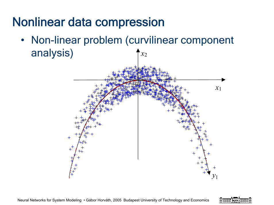
Nonlinear data compression
• Non-linear problem (curvilinear component analysis)
x1
y1
x2

Neural Networks for System Modeling • Gábor Horváth, 2005 Budapest University of Technology and Economics
ICA networks
• Such linear transformation is looked for that restores the original components from mixed observations
• Many different approaches have been developed
depending on the definition of independence
(entropy, mutual information, Kullback-Leibleir information,non-Gaussianity)
• The weights can be obtained using nonlinear network (during training)
• Nonlinear version of the Oja rule
Neural Networks for System Modeling • Gábor Horváth, 2005 Budapest University of Technology and Economics
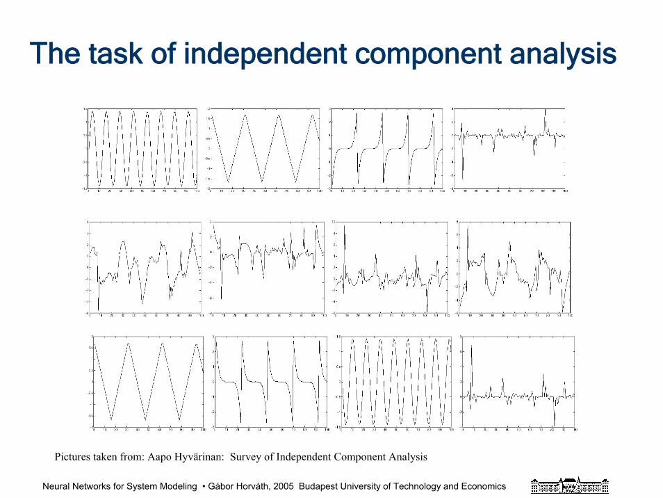
The task of independent component analysis
Pictures taken from: Aapo Hyvärinan: Survey of Independent Component Analysis
Neural Networks for System Modeling • Gábor Horváth, 2005 Budapest University of Technology and Economics
References and further readingsBrown, M. - Harris, C.J. and Parks, P "The Interpolation Capability of the Binary CMAC", Neural Networks, Vol. 6, pp. 429-440, 1993
Brown, M. and Harris, C.J. "Neurofuzzy Adaptive Modeling and Control" Prentice Hall, New York, 1994.
Hassoun, M. H.: "Fundamentals of Artificial Neural Networks", MIT Press, Cambridge, MA. 1995.
Haykin, S.: "Neural Networks. A Comprehensive Foundation" Prentice Hall, N. J.1999.
Hertz, J. - Krogh, A. - Palmer, R. G. "Introduction to the Theory of Neural Computation", Addison-Wesley Publishing Co. 1991.
Horváth, G. "CMAC: Reconsidering an Old Neural Network" Proc. of the Intelligent Control Systems and Signal Processing, ICONS 2003, Faro, Portugal. pp. 173-178, 2003.
Horváth, G. "Kernel CMAC with Improved Capability" Proc. of the International Joint Conference on Neural Networks, IJCNN’2004, Budapest, Hungary. 2004.
Lane, S.H. - Handelman, D.A. and Gelfand, J.J "Theory and Development of Higher-Order CMAC Neural Networks", IEEE Control Systems, Vol. Apr. pp. 23-30, 1992.
Miller, T.W. III. Glanz, F.H. and Kraft, L.G. "CMAC: An Associative Neural Network Alternative to Backpropagation" Proceedings of the IEEE, Vol. 78, pp. 1561-1567, 1990
Szabó, T. and Horváth, G. "Improving the Generalization Capability of the Binary CMAC” Proc. of the International Joint Conference on Neural Networks, IJCNN’2000. Como, Italy, Vol. 3, pp. 85-90, 2000.

Neural Networks for System Modeling • Gábor Horváth, 2005 Budapest University of Technology and Economics
Learning
Neural Networks for System Modeling • Gábor Horváth, 2005 Budapest University of Technology and Economics
Learning in neural networks
• Learning: parameter estimation
– supervised learning, learning with a teacher
x, y, d training set:
– unsupervised learning, learning without a teacher
x, y
– analytical learning
Piii 1, =dx
Neural Networks for System Modeling • Gábor Horváth, 2005 Budapest University of Technology and Economics
Supervised learning
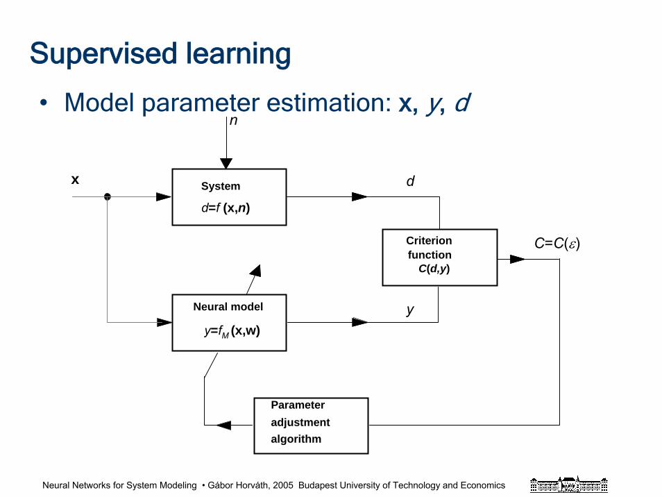
• Model parameter estimation: x, y, dn
d
y
C=C(ε)Criterion
C(d,y)
Neural model
Parameter
algorithm
System
function
adjustment
x
d=f (x,n)
y=fM (x,w)
Neural Networks for System Modeling • Gábor Horváth, 2005 Budapest University of Technology and Economics
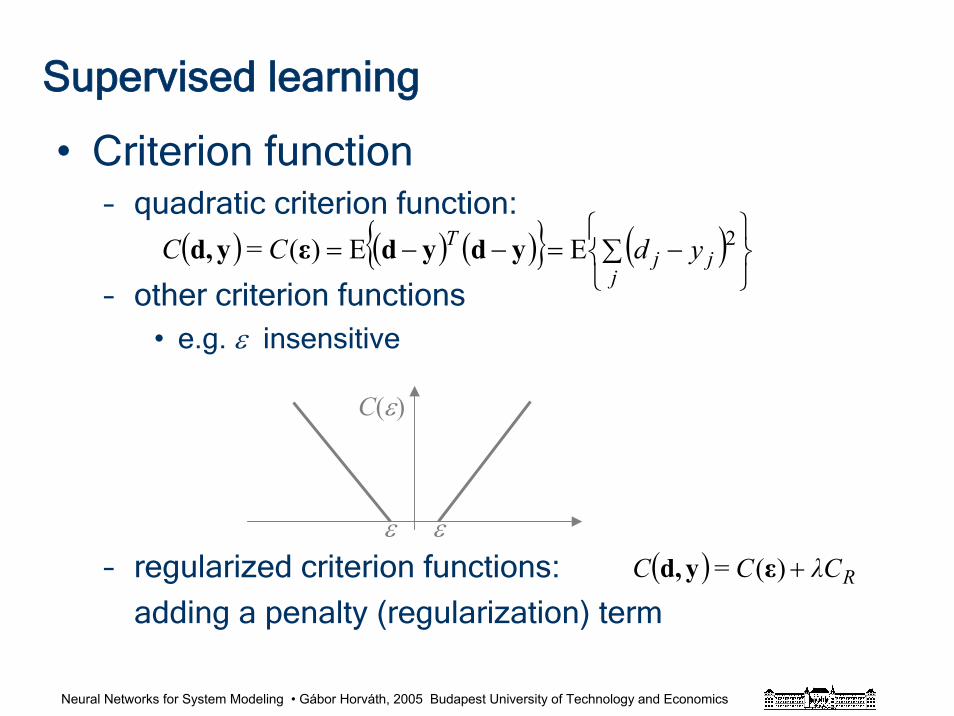
Supervised learning
• Criterion function– quadratic criterion function:
– other criterion functions• e.g. ε insensitive
– regularized criterion functions:
adding a penalty (regularization) term
( ) ( ) ( ) ( )⎭⎬⎫
⎩⎨⎧∑ −=−−=j
jjT ydCC 2EE)(= ydydεyd,
( ) RλCCC +)(= εyd,εε
C(ε)
Neural Networks for System Modeling • Gábor Horváth, 2005 Budapest University of Technology and Economics
Supervised learning
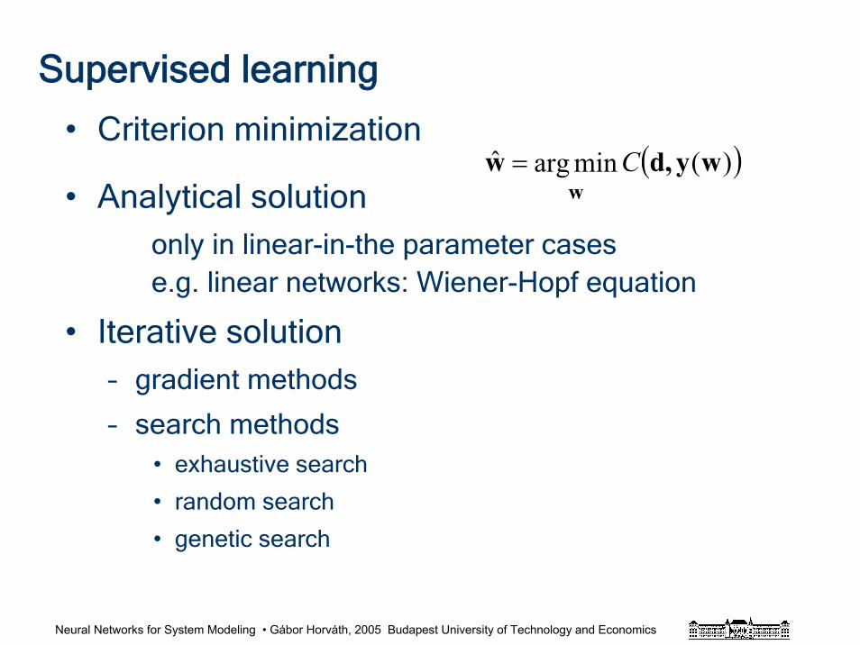
• Criterion minimization
• Analytical solutiononly in linear-in-the parameter casese.g. linear networks: Wiener-Hopf equation
• Iterative solution– gradient methods
– search methods• exhaustive search
• random search
• genetic search
( ))(minargˆ wyd,ww
C=
Neural Networks for System Modeling • Gábor Horváth, 2005 Budapest University of Technology and Economics
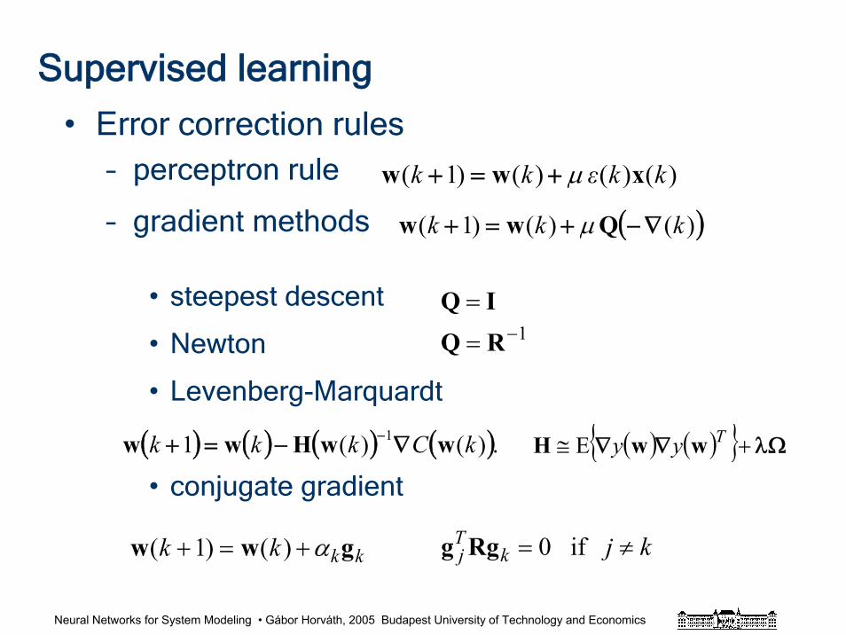
Supervised learning
• Error correction rules– perceptron rule
– gradient methods
• steepest descent
• Newton
• Levenberg-Marquardt
• conjugate gradient
( ))()()1( kkk ∇−+=+ Qww μ
IQ =1−= RQ
( ) ( ) ( ) ( ).)()(1 1 kCkkk wwHww ∇−=+ − ( ) ( ) Ωλ∇∇ +≅ Tyy wwH E
)()()()1( kkεkk xww μ+=+
kkkk gww α+=+ )()1( kjkTj ≠= if0Rgg
Neural Networks for System Modeling • Gábor Horváth, 2005 Budapest University of Technology and Economics
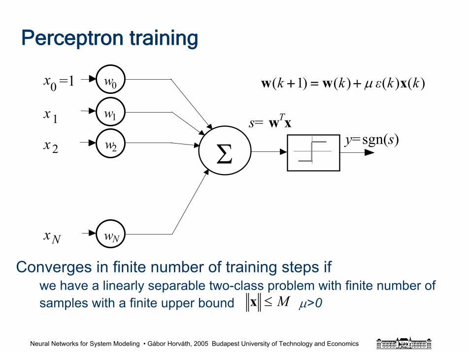
Perceptron training
=1
x1
x2
xN
0
y=sgn(s)
w0
s= wTxw1
w2
wN
x
Σ
)()()()1( kkεkk xww μ+=+
Converges in finite number of training steps if we have a linearly separable two-class problem with finite number of samples with a finite upper bound μ>0M≤x
Neural Networks for System Modeling • Gábor Horváth, 2005 Budapest University of Technology and Economics
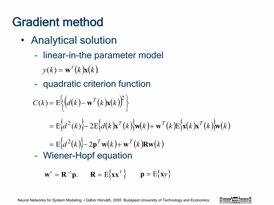
Gradient method
• Analytical solution– linear-in-the parameter model
– quadratic criterion function
– Wiener-Hopf equation
( ) ( ).)( kkky T xw=
( ) ( ) ( )( )
( ) ( ) ( ) ( ) ( ) ( ) ( )
( ) ( ) ( ) ( )kkkkd
kkkkkkkdkd
kkkdkC
TT
TTT
T
Rwwwp
wxxwwx
xw
+−=
+−=
⎭⎬⎫
⎩⎨⎧ −=
2E
EE2)(E
E)(
2
2
2
.1pRw −∗ = TxxR E= yxp E=
Neural Networks for System Modeling • Gábor Horváth, 2005 Budapest University of Technology and Economics
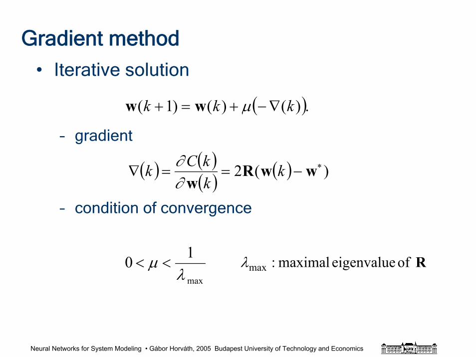
Gradient method
• Iterative solution
– gradient
– condition of convergence
( ).)()()1( kkk ∇−+=+ μww
( ) ( )( ) ( ) )(2 ∗−==∇ wwR
wk
kkCk
∂∂
max
10λ
μ << Rof eigenvalue maximal:maxλ
Neural Networks for System Modeling • Gábor Horváth, 2005 Budapest University of Technology and Economics
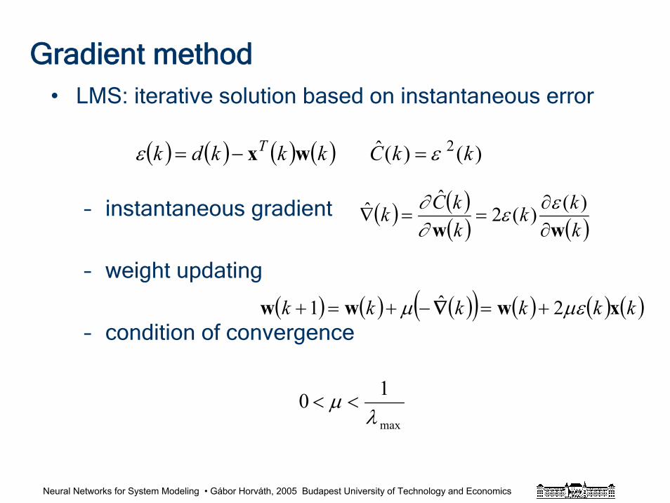
Gradient method• LMS: iterative solution based on instantaneous error
– instantaneous gradient
– weight updating
– condition of convergence
( ) ( )( ) ( )k
kkkkCk
ww ∂∂
==∇)()(2
ˆˆ εε∂∂
max
10λ
μ <<
( ) ( ) ( ) ( ) )()(ˆ 2 kkCkkkdk T εε =−= wx
( ) ( ) ( )( ) ( ) ( )kkkkk xwww μεμ 2ˆ1 +=−+=+ ∇ ( )k
Neural Networks for System Modeling • Gábor Horváth, 2005 Budapest University of Technology and Economics
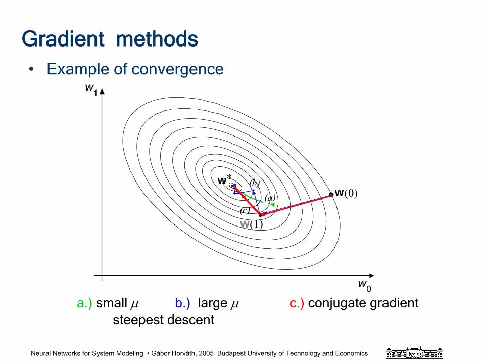
Gradient methods• Example of convergence
a.) small μ b.) large μ c.) conjugate gradientsteepest descent
0
ww
w1
w
(0)*
(1)w
(a)(b)
(c)
Neural Networks for System Modeling • Gábor Horváth, 2005 Budapest University of Technology and Economics
Gradient methods
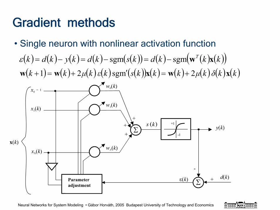
• Single neuron with nonlinear activation function
( ) ( ) ( ) ( ) ( )( ) ( ) ( ) ( )( )kkkdkskdkykdk T xwsgmsgm −=−=−=ε
( ) ( ) ( ) ( ) ( )( ) ( ) ( ) ( ) ( ) ( )kkδkμkkkskεkμkk xwxww 2msg21 +=′+=+
Parameter adjustment
Neural Networks for System Modeling • Gábor Horváth, 2005 Budapest University of Technology and Economics
Gradient methods
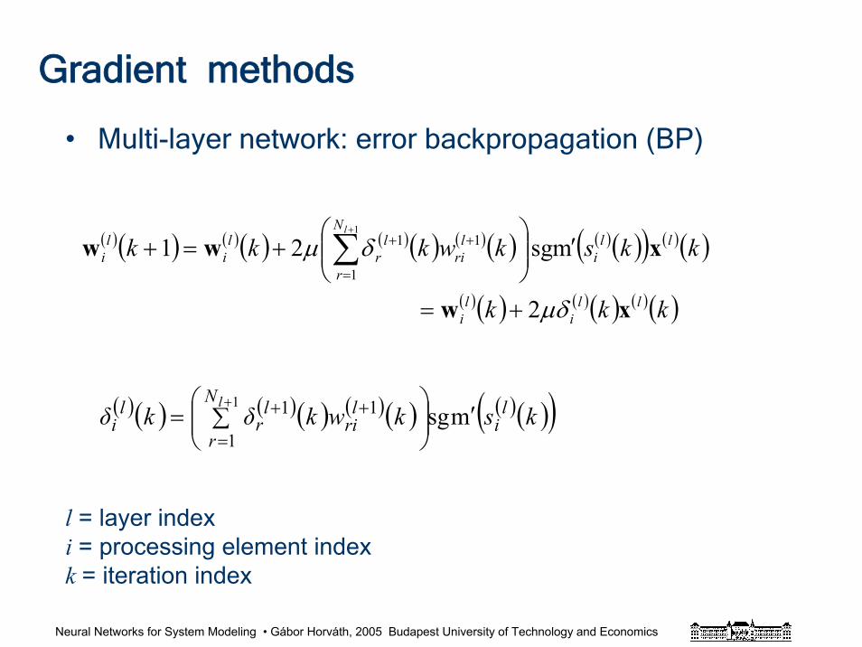
• Multi-layer network: error backpropagation (BP)
( )( ) ( )( ) ( )( ) ( )( ) ( )( )( ) ( )( )
( )( ) ( )( ) ( )( )kkk
kkskwkkk
lli
li
lli
N
r
lri
lr
li
li
l
xw
xww
μδ
δμ
2
msg211
1
11
+=
′⎟⎟⎠
⎞⎜⎜⎝
⎛+=+ ∑
+
=
++
( )( ) ( )( ) ( )( ) ( )( )( )kskwkδkδ li
N
r
lri
lr
li
lmsg
1
1
11 ′⎟⎟⎠
⎞⎜⎜⎝
⎛∑=
+
=
++
l = layer indexi = processing element indexk = iteration index
Neural Networks for System Modeling • Gábor Horváth, 2005 Budapest University of Technology and Economics
d
d
d
+
+
_
_
_
+
+
+
+y
1
2y
yn
ε
ε
ε2
2
1
1
n
n
x
x
Π Π
xx
x
x
y = x
x(1)2
updating updating
(2)
(2)
μ μ2x
x
(1)
(1) (2)
x =oo(2)
Σ
Σ
Σ
Σ
Σ
ΣW
W
(2)(1)
(1)
δδ (2) (2)(1)
W
W W
1 1x =
x
x
x
x
1
2
3
N
(1)
(1)
(1)
(1)
(1) f(.) f(.)
f(.)
f(.) f(.)
f(.)
f'(.) f'(.)
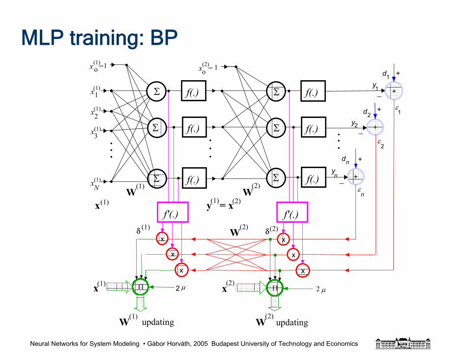
MLP training: BP
Neural Networks for System Modeling • Gábor Horváth, 2005 Budapest University of Technology and Economics
Designing of an MLP
• important questions– the size of the network (model order: number of
layers, number of hidden units)
– the value of the learning rate, μ– initial values of the parameters (weights)
– validation, cross validation learning and testing set selection
– the way of learning, batch or sequential
– stopping criteria
Neural Networks for System Modeling • Gábor Horváth, 2005 Budapest University of Technology and Economics
Designing of an MLP
• The size of the network: the number of hidden units (model order)– theoretical results: upper limits
• Practical approaches: two different strategies– from simple to complex
• adding new neurons
– from complex to simple• pruning
– regularization
– (OBD, OBS, etc)
Neural Networks for System Modeling • Gábor Horváth, 2005 Budapest University of Technology and Economics
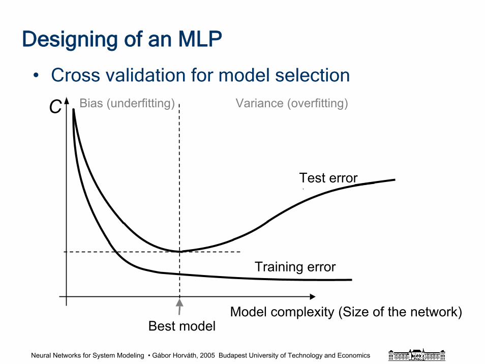
Designing of an MLP
• Cross validation for model selection
C
Model complexity (Size of the network)
Test error
Training error
Best model
Bias (underfitting) Variance (overfitting)
Neural Networks for System Modeling • Gábor Horváth, 2005 Budapest University of Technology and Economics
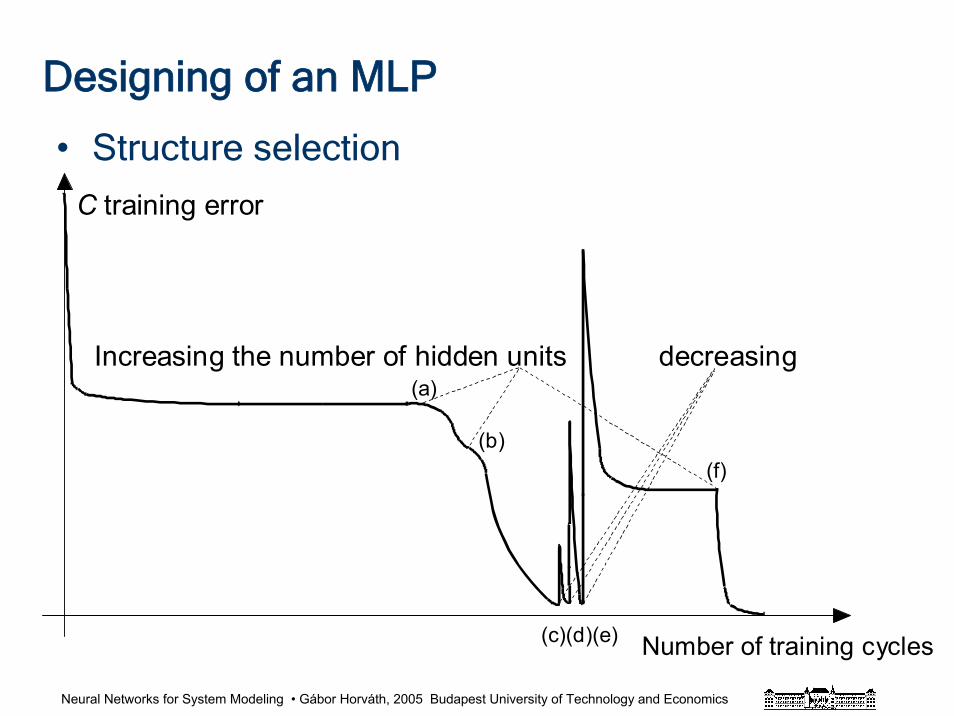
Designing of an MLP
• Structure selection
C training error
Number of training cycles
Increasing the number of hidden units decreasing (a)
(b)
(c)(d)(e)
(f)
Neural Networks for System Modeling • Gábor Horváth, 2005 Budapest University of Technology and Economics
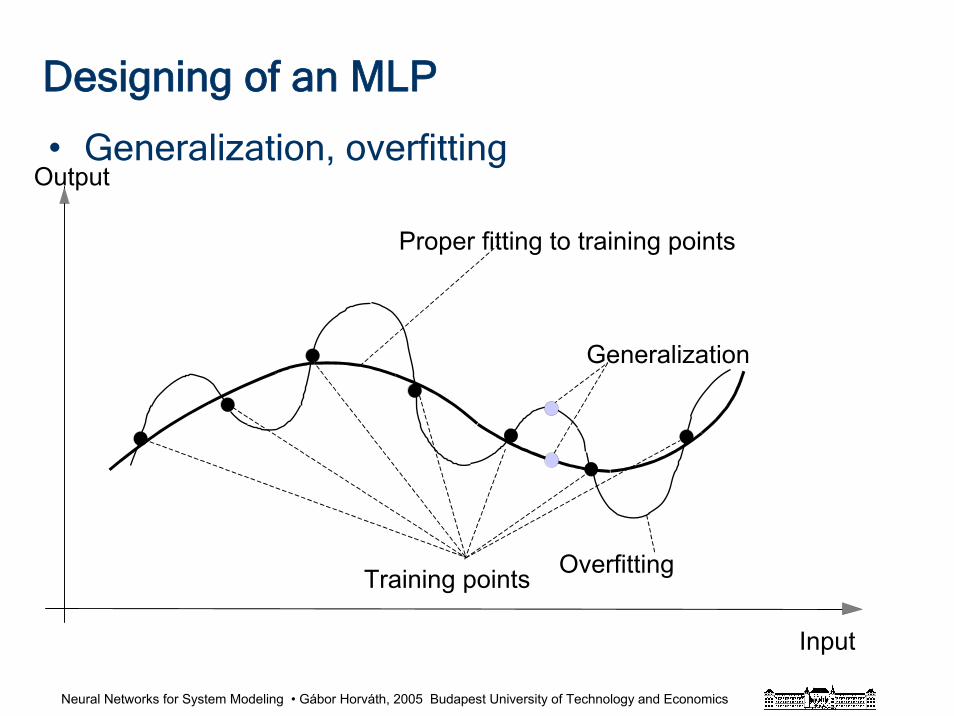
Output
Proper fitting to training points
Generalization
Training points Overfitting
Input
Designing of an MLP
• Generalization, overfitting
Neural Networks for System Modeling • Gábor Horváth, 2005 Budapest University of Technology and Economics
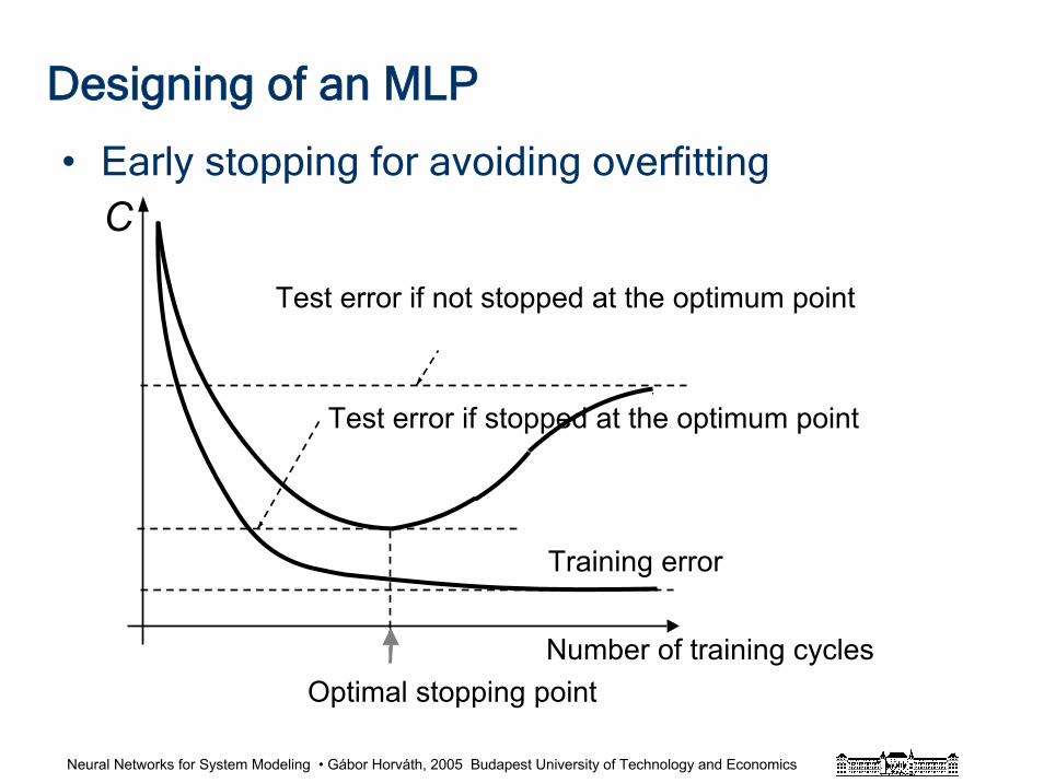
Designing of an MLP
• Early stopping for avoiding overfittingC
Number of training cycles
Test error if stopped at the optimum point
Test error if not stopped at the optimum point
Training error
Optimal stopping point
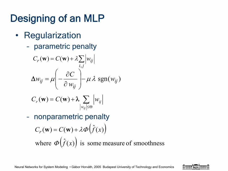
Neural Networks for System Modeling • Gábor Horváth, 2005 Budapest University of Technology and Economics
Designing of an MLP
• Regularization– parametric penalty
– nonparametric penalty
∑+=ji
ijr wCC,
)()( λww
)(sgn ijij
ij wwCw λμμ −⎟
⎟⎠
⎞⎜⎜⎝
⎛
∂∂
−=Δ
∑Θ≤
+=ijw
ijr wCC λ)()( ww
( )( ) smoothness of measure some is)(ˆ where
)(ˆ)()(
xf
xfCCr
Φ
Φλ+= ww
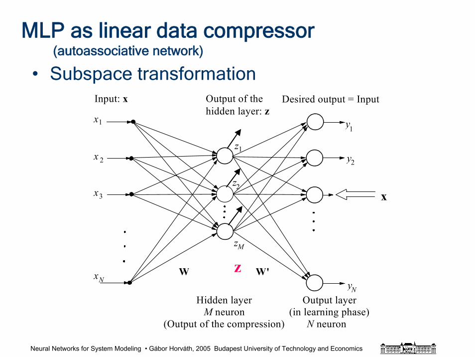
Neural Networks for System Modeling • Gábor Horváth, 2005 Budapest University of Technology and Economics
MLP as linear data compressor(autoassociative network)
• Subspace transformation
Desired output = Input Input: x Output of the hidden layer: z
x
x
x
x W
Hidden layer Output layer M neuron (in learning phase) (Output of the compression) N neuron
N
1
2
3 x
W'
y
y
y
1
2
N
z
z
z
1
2
M
z
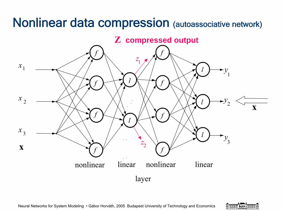
Neural Networks for System Modeling • Gábor Horváth, 2005 Budapest University of Technology and Economics
Nonlinear data compression (autoassociative network)
x
x
x
1
2
3
x
nonlinear linear nonlinear linear
layer
y
y
1
2
z1
2
Z compressed output
f
f
f
f
f
f
f
f
l
ll
l
l yzx 3
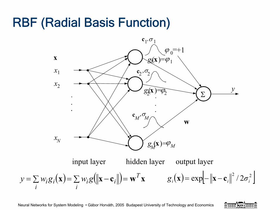
Neural Networks for System Modeling • Gábor Horváth, 2005 Budapest University of Technology and Economics
( ) ( ) xwcxx T
iii
iii gwgwy =∑ −=∑= ( ) [ ]22 2/exp iii σg cxx −−=
RBF (Radial Basis Function)σ
g =
x
x1
2
N
y
+1
w
c
c
c
Σ
1,
,σ
,σ
2
M M
input layer hidden layer output layer
x
ϕ =0
g =
g =
2
1
1 1
2 2
M M
( )
( )
( )
x
x
x
x ϕ
ϕ
ϕ
Neural Networks for System Modeling • Gábor Horváth, 2005 Budapest University of Technology and Economics
RBF training
• Linear-in-the parameter structure– analytical solution
– LMS
• Cetres (nonlinear-in-the-parameters)– K-means
– clustering
– unsupervised learning
Neural Networks for System Modeling • Gábor Horváth, 2005 Budapest University of Technology and Economics
Designing of an RBF
• Important questions– the size of the network (number of hidden units)
(model order)
– the value of learning rate, μ– initial values of parameters (centres, weights)
– validation, learning and testing set selection
– the way of learning, batch or sequential
– stopping criteria
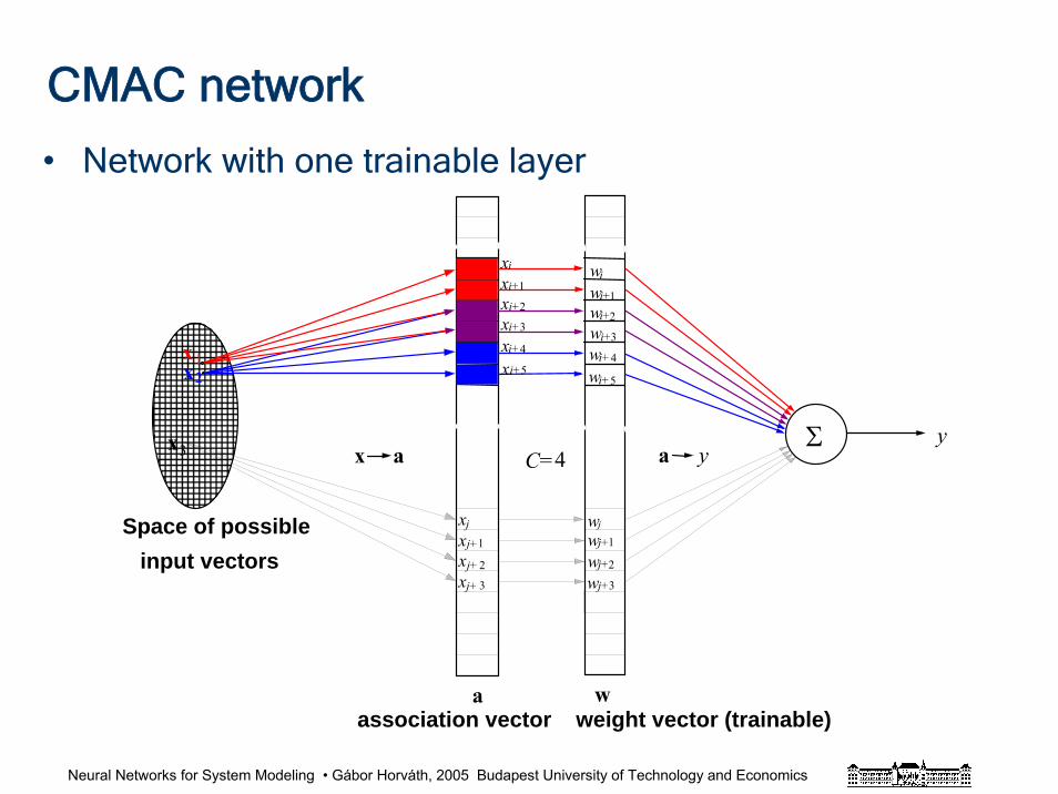
Neural Networks for System Modeling • Gábor Horváth, 2005 Budapest University of Technology and Economics
CMAC network
• Network with one trainable layer
Σ
Space of possibleinput vectors
xx
i+
i+3
x a a y
y
wwwww
i
i+
i+
i+
2
1
3
C=4
waassociation vector weight vector (trainable)
x1
2
i+
i+
4
5x
x
2
3
xx
xx
j+
j+
1
2
3
j j
j+
w
wwww
j+
j+
j+
1
3
2
xi
x
x
x
i+1
i+
i+
4
5
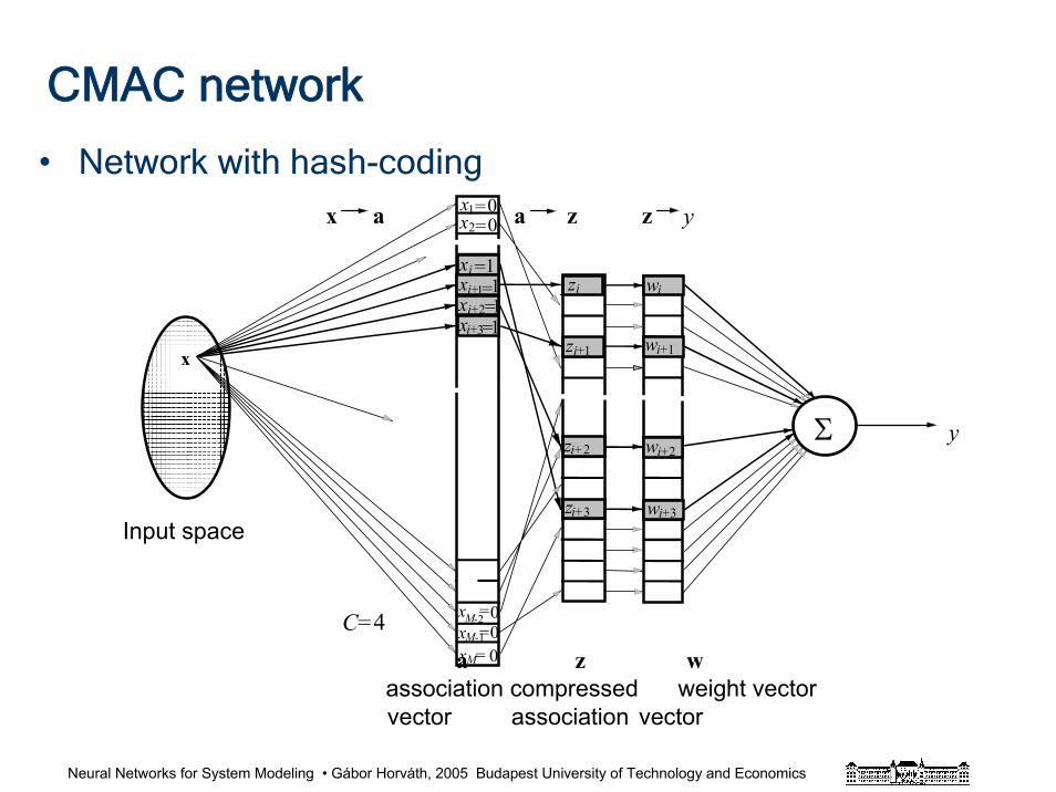
Neural Networks for System Modeling • Gábor Horváth, 2005 Budapest University of Technology and Economics
CMAC network
• Network with hash-coding
a wzassociation compressed weight vectorvector association vector
x =
Σ
xx
==
Input space
x
xxxi+
1
===
111
00
x =x =M
M
0
00
z
y
y
M
-1-2
12
i+
i+
2
C=4
xi+3=1z
i+
i+
i+z
w
w
w
w
i+
i+
i+
z
z
2
3 3
2
1 1
ii i
x a a z
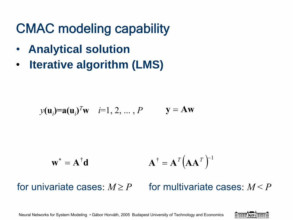
Neural Networks for System Modeling • Gábor Horváth, 2005 Budapest University of Technology and Economics
• Analytical solution
y(ui)=a(ui)Tw i=1, 2, ... , P
dAw †=∗ ( ) 1† −= TT AAAA
Awy =
CMAC modeling capability
for univariate cases: M ≥ P for multivariate cases: M < P
• Iterative algorithm (LMS)
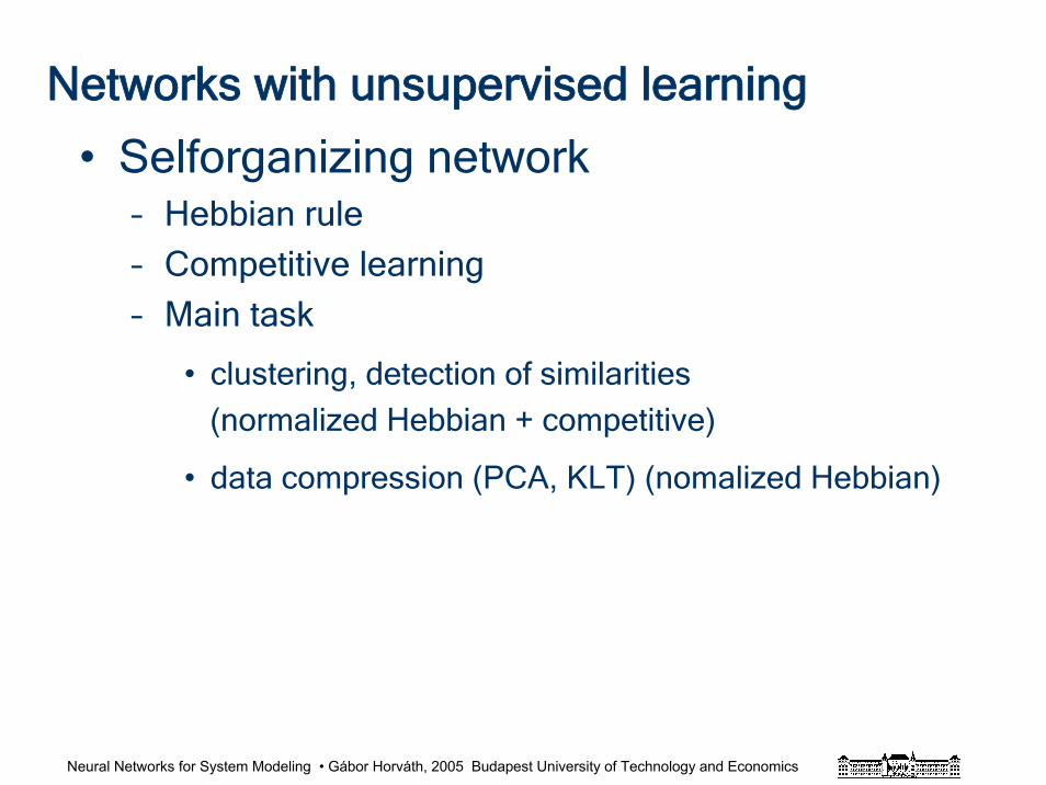
Neural Networks for System Modeling • Gábor Horváth, 2005 Budapest University of Technology and Economics
Networks with unsupervised learning
• Selforganizing network– Hebbian rule
– Competitive learning
– Main task
• clustering, detection of similarities
(normalized Hebbian + competitive)
• data compression (PCA, KLT) (nomalized Hebbian)
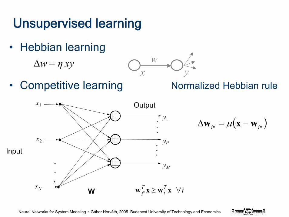
Neural Networks for System Modeling • Gábor Horváth, 2005 Budapest University of Technology and Economics
Unsupervised learning
• Hebbian learning
• Competitive learning
xyηw =Δ wyx
Output
Input
x
y
y
y
WxN
1
x 1
i*2
M
iTi
Ti ∀≥∗ xwxw
( )∗∗ −=Δ ii wxw μ
Normalized Hebbian rule
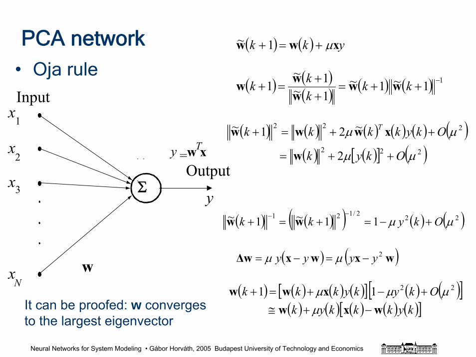
Neural Networks for System Modeling • Gábor Horváth, 2005 Budapest University of Technology and Economics
PCA network
• Oja rule
( ) ( )wxwxΔw 2yyyy −=−= μμ
( ) ( )( ) ( ) ( ) 11~1~
1~1~
1 −++=++
=+ kkkkk ww
www
( ) ( ) ( ) ( ) ( ) ( )( ) ( )[ ] ( )222
222
2
~21~
μμ
μμ
Okyk
Okykkkk T
++=
++=+
w
xwww
( ) ( )( ) ( ) ( )222/121 11~1~ μμ Okykk +−=+=+−− ww
( ) ( ) ( ) ( )[ ] ( ) ( )[ ]( ) ( ) ( ) ( ) ( )[ ]kykkkyk
Okykykkkwxw
xww−+≅
+−+=+μ
μμμ
11 22
=w xTyOutput
Inputx
x
x
x
Σy
1
2
3
Nw
( ) ( ) ykk xww μ+=+ 1~
It can be proofed: w converges to the largest eigenvector
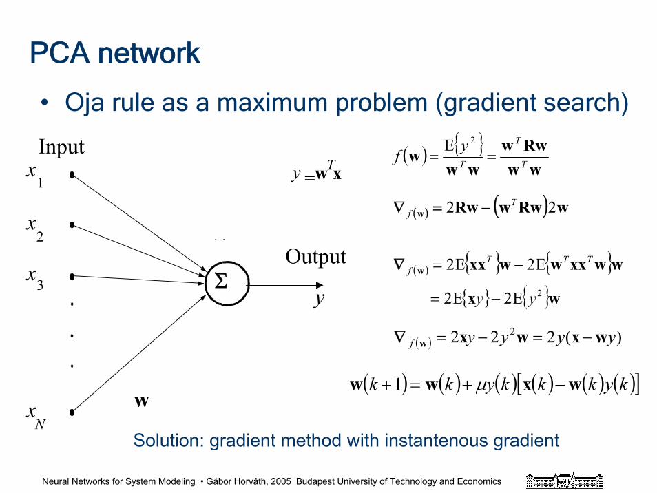
Neural Networks for System Modeling • Gábor Horváth, 2005 Budapest University of Technology and Economics
PCA network
• Oja rule as a maximum problem (gradient search)
( ) ww
Rwwww
w T
T
T
yf ==2E
( ) ( ) wRwwRww 22 Tf −=∇
( ) wx
wwxxwwxxw
2E2E2
E2E2
yy
TTTf
−=
−=∇
( ) )(222 2 yyyyf wxwxw −=−=∇
Output
Inputx
x
x
x
=w xT
Σy
y1
2
3
Nw
Solution: gradient method with instantenous gradient
( ) ( ) ( ) ( ) ( ) ( )[ ]kykkkykk wxww −+=+ μ1

Neural Networks for System Modeling • Gábor Horváth, 2005 Budapest University of Technology and Economics
PCA networks
• GHA network (Sanger network)( )1
21
)1(11 wxw yy −= μΔ
( ) 11)1(
1)1(
1)1()2( wxwxwxx yT −=−=
( )( )2
22121
)1(2
222
)2(22
wwx
wxw
yyyy
yy
−−
=−=Δ
μ
μ
( )( )
=
...=
21
1
)1(
221
)1(
2)1(
⎟⎟⎠
⎞⎜⎜⎝
⎛−−
−−−
−=Δ
∑−
=ii
i
jijii
iiii
iiii
yyyy
yyyy
yy
wwx
wwx
wxw
μ
μ
μ
( )[ ]WyyyxW TT LT−= ηΔ
Output
Inputx
x
x
x
y
y
y
WN
1
12
23
M
Oja rule + Gram-Schmidt orthogolarization
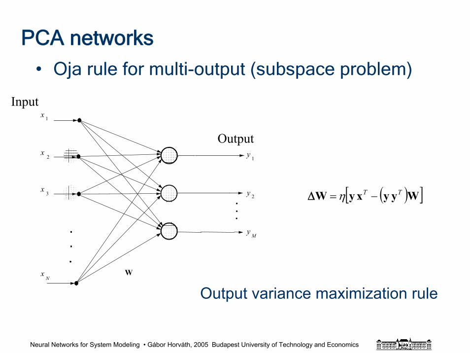
Neural Networks for System Modeling • Gábor Horváth, 2005 Budapest University of Technology and Economics
PCA networks
• Oja rule for multi-output (subspace problem)
Output
Inputx
x
x
x
y
y
y
WN
1
12
23
M
( )[ ]WyyxyW TT −= ηΔ
Output variance maximization rule
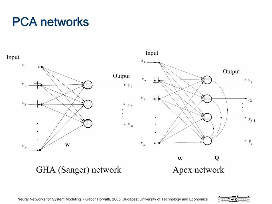
Neural Networks for System Modeling • Gábor Horváth, 2005 Budapest University of Technology and Economics
PCA networks
Output
Inputx
x
x
x
y
y
W Q
N
1
2
23
1
1
y
y
j-
j
Output
Inputx
x
x
x
y
y
y
WN
1
12
23
M
GHA (Sanger) network Apex network
Neural Networks for System Modeling • Gábor Horváth, 2005 Budapest University of Technology and Economics
ICA networks
• Such linear transformation is looked for that restores the original components from mixed observations
• Many different approaches have been developed
depending on the definition of independence
(entropy, mutual information, Kullback-Leibleir information,non-Gaussianity)
• The weights can be obtained using nonlinear network (during training)
• Nonlinear version of the Oja rule
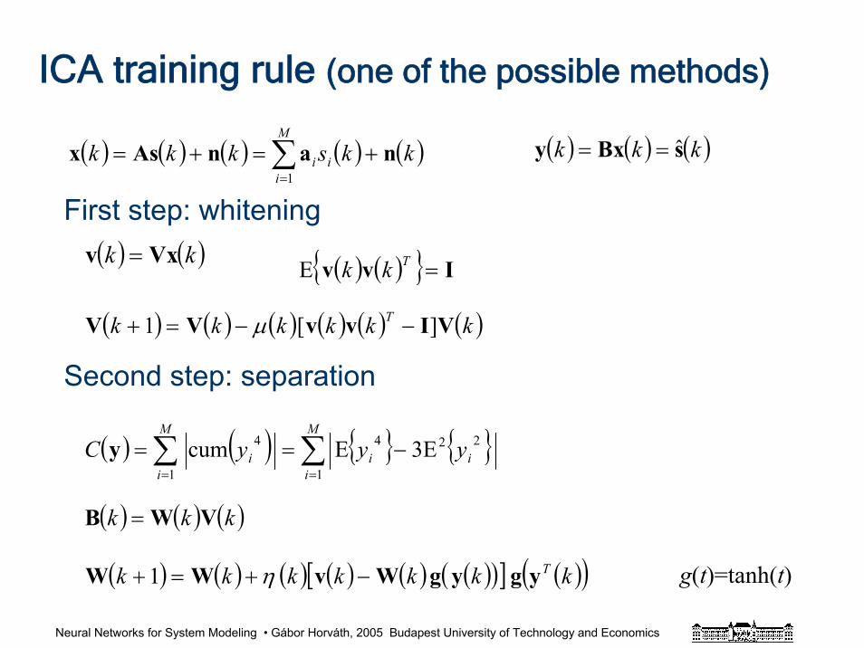
Neural Networks for System Modeling • Gábor Horváth, 2005 Budapest University of Technology and Economics
ICA training rule (one of the possible methods)
( ) ( ) ( ) ( ) ( ) ( )( )[ ] ( )( )kkkkkkk TygygWvWW −+=+ η1
( ) ( ) ( ) ( ) ( )kkskkk i
M
ii nanAsx +=+= ∑
=1
( ) ( ) ∑∑==
−==M
iii
M
ii yyyC
1
224
1
4 E3Ecumy
( ) ( ) ( )kkk sBxy ˆ==
( ) ( ) ( ) ( ) ( ) ( )kkkkkk T VIvvVV ][1 −−=+ μ
( ) ( ) ( )kkk VWB =
( ) ( )kk Vxv = ( ) ( ) Ivv =TkkE
First step: whitening
Second step: separation
g(t)=tanh(t)
Neural Networks for System Modeling • Gábor Horváth, 2005 Budapest University of Technology and Economics
Networks with unsupervised learning
• clustering
• detection of similarities
• data compression (PCA, KLT)
• Independent component analysis (ICA)
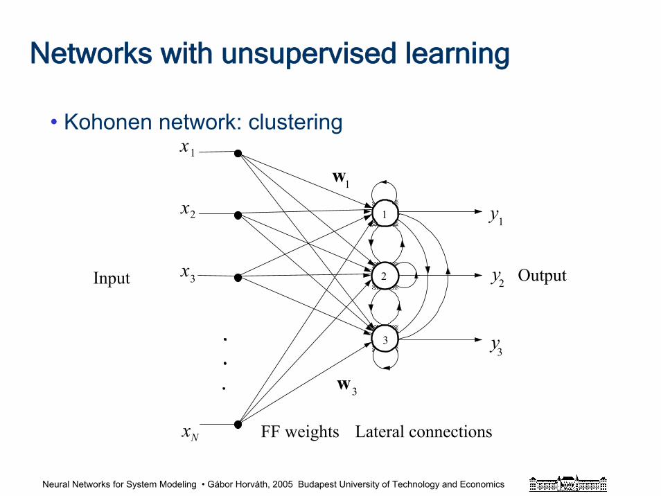
Neural Networks for System Modeling • Gábor Horváth, 2005 Budapest University of Technology and Economics
Networks with unsupervised learning
• Kohonen network: clustering
OutputInput
x
x
x FF weights
y
y
y
x
Lateral connections
3
N
2
2
1
3
w
w
1
3
1
2
3
1
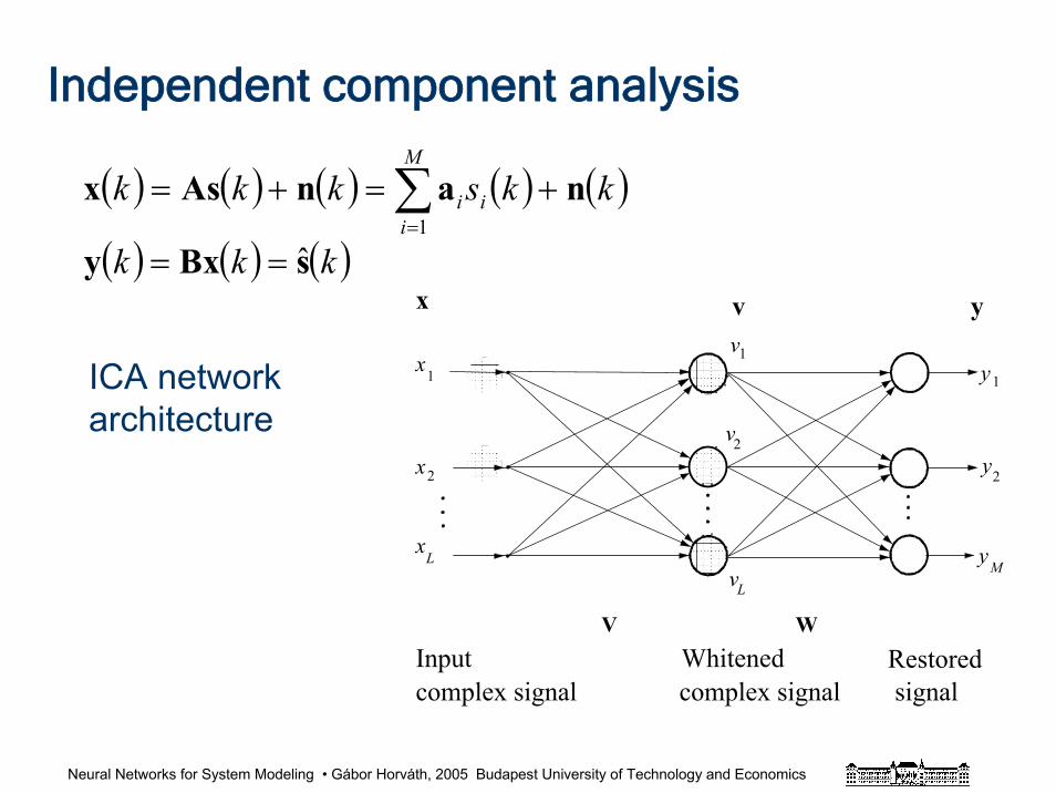
Neural Networks for System Modeling • Gábor Horváth, 2005 Budapest University of Technology and Economics
Independent component analysis
( ) ( ) ( ) ( ) ( )kkskkk i
M
ii nanAsx +=+= ∑
=1
( ) ( ) ( )kkk sBxy ˆ==
RestoredInput Whitened
x
x
x
V
1
L
x
W
y1
v yv
v
v
1
2
L
2 y
yM
2
complex signal complex signal signal
ICA network architecture
Neural Networks for System Modeling • Gábor Horváth, 2005 Budapest University of Technology and Economics
References and further readingsDiamantaras, K. I .- Kung, S. Y. "Principal Component Neural Networks Theory and Applications", John Wiley and Sons, New York. 1996.
Girolami, M - Fyfe, C. "Higher Order Cumulant Maximisation Using Nonlinear Hebbian and Anti-Hebbian Learning for Adaptive Blind Separation of Source Signals", Proc. of the IEEE/IEE International Workshop on Signal and Image Processing, IWSIP-96, Advances in Computational Intelligence, Elsevier publishing, pp. 141 - 144, 1996.
Hassoun, M. H.: "Fundamentals of Artificial Neural Networks", MIT Press, Cambridge, MA. 1995.
Haykin, S.: "Neural Networks. A Comprehensive Foundation" Prentice Hall, N. J.1999. Hertz, J. - Krogh, A. - Palmer, R. G. "Introduction to the Theory of Neural Computation", Addison-Wesley Publishing Co. 1991.
Karhunen, J. - Joutsensalo, J. "Representation and Separation of Signals using Nonlinear PCA Type Learning", Neural Networks, Vol. 7. No. 1. 1994. pp. 113-127.
Karhunen, J. - Hyvärinen, A. - Vigario, R. - Hurri, J. - and Oja, E. "Applications of Neural Blind Source Separation to Signal and Image Processing", Proceedings of the IEEE 1997 International Conference on Acoustics, Speech, and Signal Processing (ICASSP'97), April 21 - 24. 1997. Munich, Germany, pp. 131-134.
Kung, S. Y. - Diamantaras, C.I. "A Neural Network Learning Algorithm for Adaptive Principal Component Extraction (APEX)", International Confer-ence on Acoustics, Speech and Signal Processing, Vol. 2. 1990. pp. 861-864.
Narendra, K. S. – Parthasaraty, K. „Gradient Methods for the Optimization of Dynamical Systems Containing Neural Networks” IEEE Trans. on Neural networks, vol. 2. No. 2. pp. 252-262. 1991.
Sanger, T. "Optimal Unsupervised Learning in a Single-layer Linear Feedforward Neural Network", Neural Networks, Vol. 2. No. 6. 1989. pp. 459-473.
Widrow, B. - Stearns, S. D. "Adaptive Signal Processing", Prentice-Hall, Englewood Cliffs, N. J. 1985.
Neural Networks for System Modeling • Gábor Horváth, 2005 Budapest University of Technology and Economics
Dynamic neural architectures
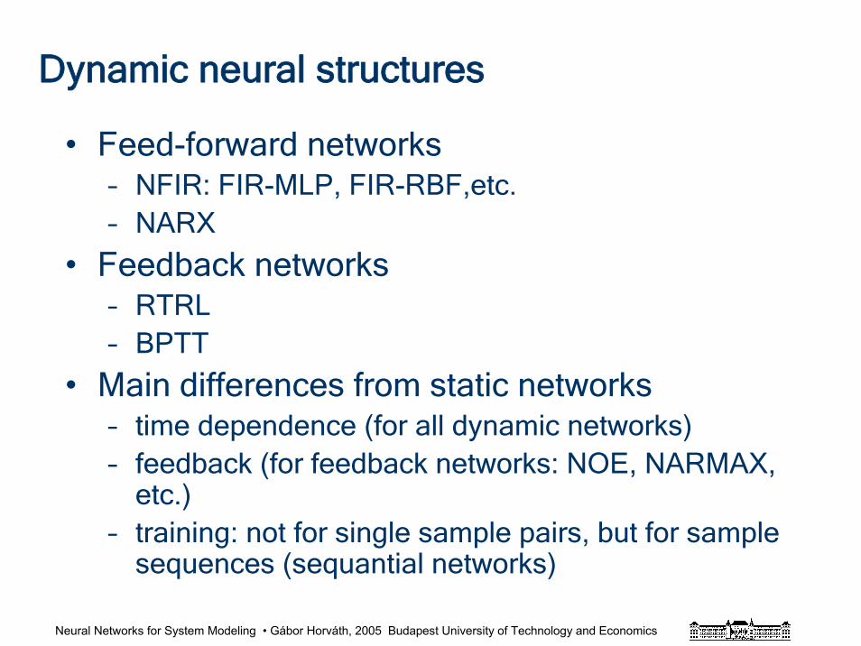
Neural Networks for System Modeling • Gábor Horváth, 2005 Budapest University of Technology and Economics
Dynamic neural structures
• Feed-forward networks– NFIR: FIR-MLP, FIR-RBF,etc.– NARX
• Feedback networks– RTRL– BPTT
• Main differences from static networks– time dependence (for all dynamic networks)– feedback (for feedback networks: NOE, NARMAX,
etc.)– training: not for single sample pairs, but for sample
sequences (sequantial networks)
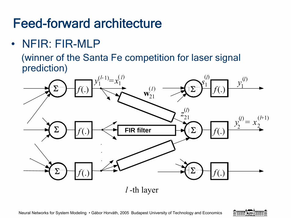
Neural Networks for System Modeling • Gábor Horváth, 2005 Budapest University of Technology and Economics
Feed-forward architecture
• NFIR: FIR-MLP (winner of the Santa Fe competition for laser signal prediction)
y =x 1 1l- l( 1) ( )
( +1)
s
z
FIR filter
(.)(.)
(.)
(.)
(.)
(.)
Σ
Σ
Σ Σ
Σ
Σ
-th layer
( )
( )1 y
y = x
1
( )
( )
2 221
l
.
.
.
ll
ll l
f f
f
f f
f
w l( )21
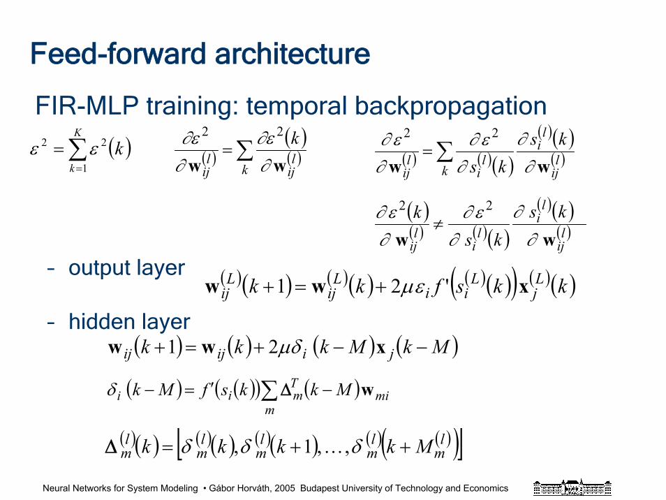
Neural Networks for System Modeling • Gábor Horváth, 2005 Budapest University of Technology and Economics
Feed-forward architecture
FIR-MLP training: temporal backpropagation
– output layer
– hidden layer( ) ( ) ( ) ( )MkMkkk jiijij −−+=+ xww μδ21
( ) ( )( ) ( ) mim
Tmii MkksfMk w∑ −′=− Δδ
( )( ) ( )( ) ( )( ) ( ) ( )( )[ ]lm
lm
lm
lm
lm Mkkkk ++= δδδ ,...,1,Δ
( )( )( )∑=
kl
ijl
ij
kww ∂
∂ε∂∂ε 22
( ) ( )( )( )( )
( )lij
li
kl
il
ij
ksks ww ∂
∂∂
ε∂∂
ε∂ ∑=22
( )( ) ( )( )
( )( )( )lij
li
li
lij
ksks
kww ∂
∂∂
ε∂∂ε∂ 22
≠
( )( ) ( )( ) ( )( )( ) ( )( )kksfkk Lj
Lii
Lij
Lij xww '21 εμ+=+
( )kK
k∑
=
=1
22 εε
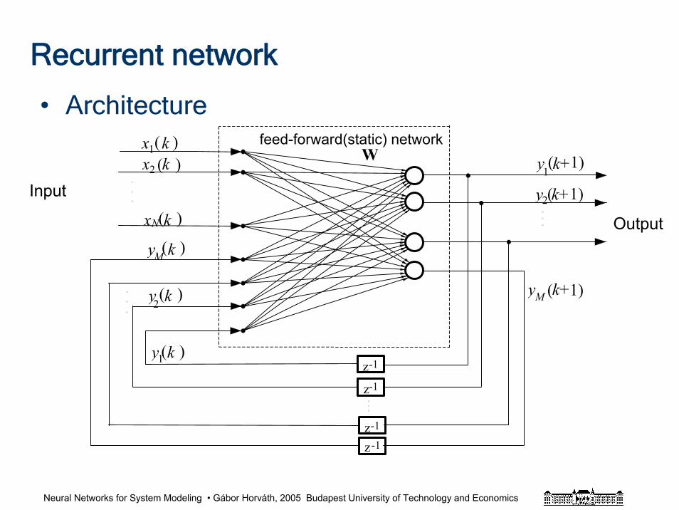
Neural Networks for System Modeling • Gábor Horváth, 2005 Budapest University of Technology and Economics
Recurrent network
• Architecture
Outputx k
x k
Inputx k
y k
y k
y k
y k+
y k+
y k+1
1
1
M
M
2
2
2
N
z
z
-1
-1
zz
-1
-1
Wfeed-forward(static) network
( 1)
( 1)
( 1)( )( )
( )
( )
( )
( )
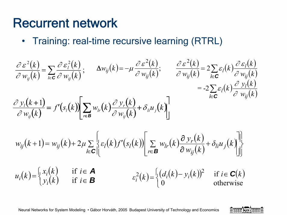
Neural Networks for System Modeling • Gábor Horváth, 2005 Budapest University of Technology and Economics
Recurrent network• Training: real-time recursive learning (RTRL)
( ) ( ) ( ) ( )( ) ( ) ( )( ) ( )∑
⎪⎭
⎪⎬⎫
⎪⎩
⎪⎨⎧
⎥⎥⎦
⎤
⎢⎢⎣
⎡∑ +′+=+
∈ ∈C Bl rjli
ij
rlrllijij kuδ
kwkykwksfkεμkwkw
∂∂21
( ) ( )( )⎩
⎨⎧
∈∈= B
Aikyikxku
ii
i ifif ( ) ( ) ( )( ) ( )
⎩⎨⎧ ∈−=
otherwise 0 if 22 kikykdkε iii
C
( )( )
( )( ) ;
22
∑∈
=Cl ij
l
ij kwk
kwk
∂ε∂
∂ε∂ ( ) ( )
( );2
kwkkw
ijij ∂
ε∂μ−=Δ( )( ) ( ) ( )
( )( ) ( )
( )kwkyk
kwkk
kwk
ij
l
ll
ij
l
ll
ij
∂∂ε
∂ε∂ε
∂ε∂
∑
∑
∈
∈=
C
C
2-=
22
( )( ) ( )( ) ( ) ( )
( ) ( ) 1⎥⎥⎦
⎤
⎢⎢⎣
⎡+′=
+ ∑∈Br
jliij
rlrl
ij
l kukwkykwksf
kwky δ
∂∂
∂∂
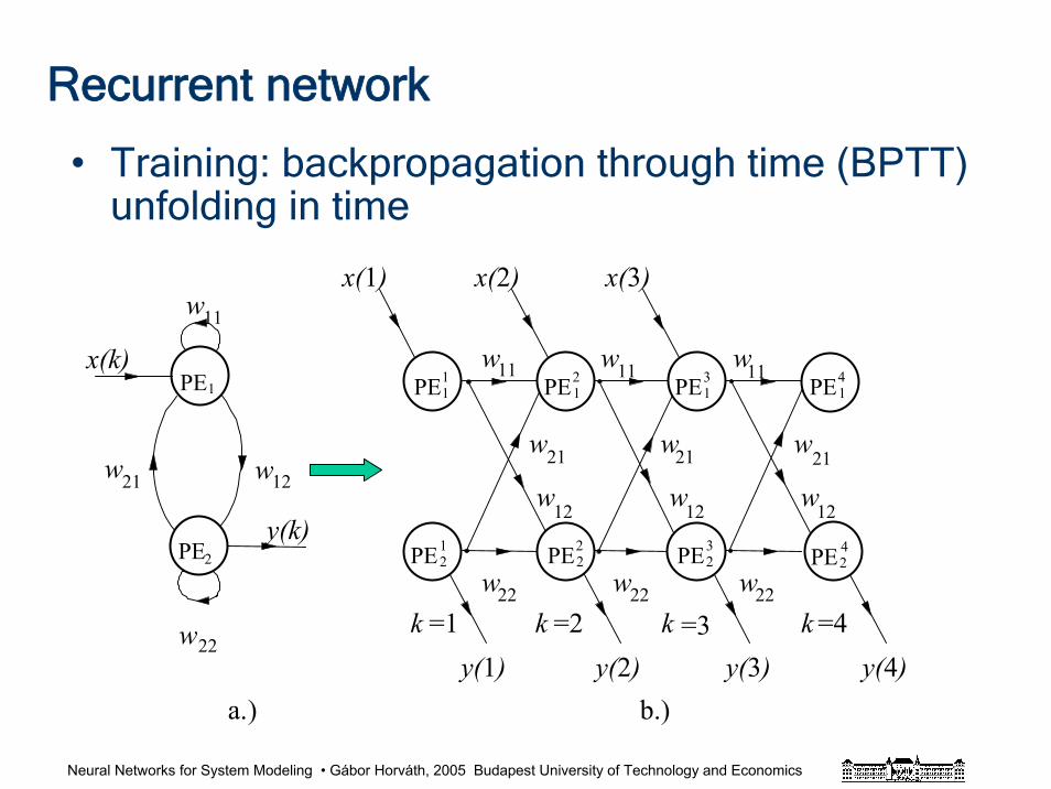
Neural Networks for System Modeling • Gábor Horváth, 2005 Budapest University of Technology and Economics
Recurrent network
• Training: backpropagation through time (BPTT)unfolding in time
a.) b.)
PE
PE
1
2
w
w w
w22
1221
11
PE1
PE2
x(k)
y(k)
k k kk =1 =2 =3 =4
w w
w w w
w w w
w w w
11 11
22 22
21 21
12 12
w
22
12
21
11
4
PE PE PE PE11
1 1 12 3 4
PE PE PE PE2 2 2 221 3 4PE2
4
x(1) x(2) x(3)
y(1) y(2) y(3) y(4)
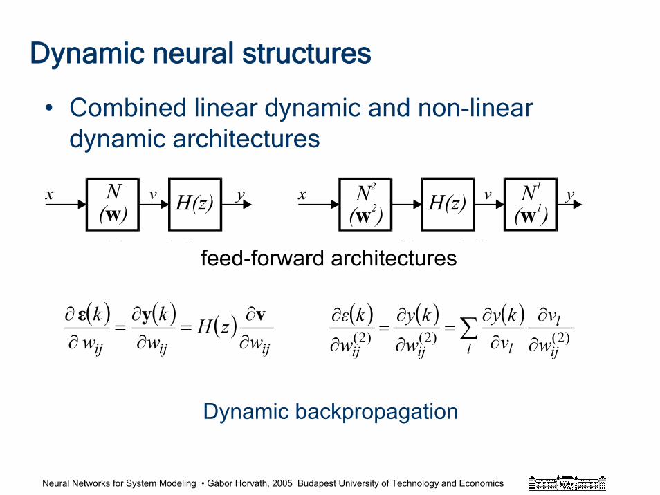
Neural Networks for System Modeling • Gábor Horváth, 2005 Budapest University of Technology and Economics
Dynamic neural structures
• Combined linear dynamic and non-linear dynamic architectures
feed-forward architectures
( ) ( ) ( )ijijij w
zHw
kw
k∂∂
=∂
∂=
∂∂ vyε ( ) ( ) ( )∑
∂
∂∂
∂=
∂
∂=
∂
∂
l ij
l
lijij wv
vky
wky
wkε
)2()2()2(
Dynamic backpropagation
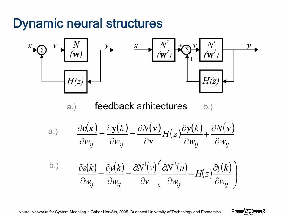
Neural Networks for System Modeling • Gábor Horváth, 2005 Budapest University of Technology and Economics
Dynamic neural structures
( ) ( ) ( ) ( ) ( ) ( ) 21
⎟⎟⎠
⎞⎜⎜⎝
⎛
∂∂
+∂
∂∂
∂=
∂∂
=∂∂
ijijijij wkyzH
wuN
vvN
wky
wkε
a.) feedback arhitectures b.)
( ) ( ) ( ) ( ) ( ) ( )ijijijij w
Nw
kzHNw
kw
k∂
∂+
∂∂
∂∂
=∂
∂=
∂∂ vy
vvyεa.)
b.)
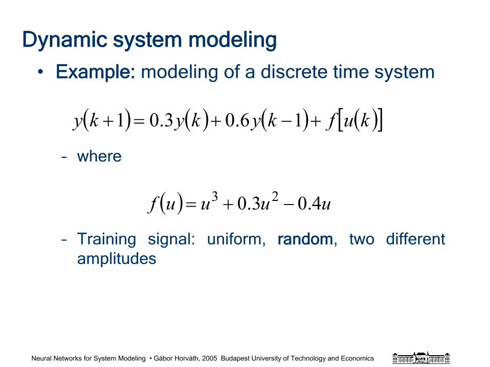
Neural Networks for System Modeling • Gábor Horváth, 2005 Budapest University of Technology and Economics
Dynamic system modeling
• Example: modeling of a discrete time system
– where
– Training signal: uniform, random, two different amplitudes
( ) ( ) ( ) ( )[ ]kufkykyky +−+=+ 16.03.01
( ) uuuuf 4.03.0 23 −+=
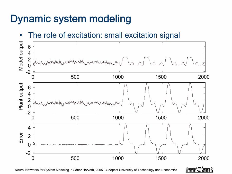
Neural Networks for System Modeling • Gábor Horváth, 2005 Budapest University of Technology and Economics
Dynamic system modeling
• The role of excitation: small excitation signal
0 500 1000 1500 2000-20246
Mod
el o
utpu
t
0 500 1000 1500 2000-20246
Plan
t out
put
0 500 1000 1500 2000-2024
Erro
r
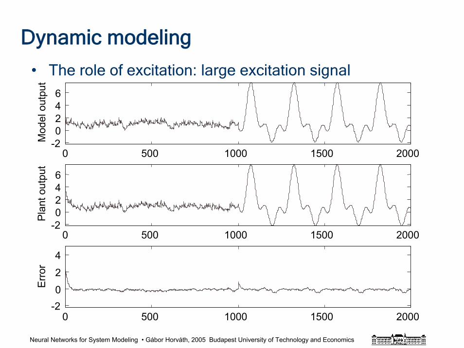
Neural Networks for System Modeling • Gábor Horváth, 2005 Budapest University of Technology and Economics
Dynamic modeling
• The role of excitation: large excitation signal
0 500 1000 1500 2000-20246
Mod
el o
utpu
t
0 500 1000 1500 2000-20246
Plan
t out
put
0 500 1000 1500 2000-2024
Erro
r
Neural Networks for System Modeling • Gábor Horváth, 2005 Budapest University of Technology and Economics
References and further readings
Hassoun, M. H.: "Fundamentals of Artificial Neural Networks", MIT Press, Cambridge, MA. 1995.
Haykin, S.: "Neural Networks. A Comprehensive Foundation" Prentice Hall, N. J.1999.
Hertz, J. - Krogh, A. - Palmer, R. G. "Introduction to the Theory of Neural Computation", Addison-Wesley Publishing Co. 1991.
Widrow, B. - Stearns, S. D. "Adaptive Signal Processing", Prentice-Hall, Englewood Cliffs, N. J. 1985.
Narendra, K. S. - Pathasarathy, K. "Identification and Control of Dynamical Systems Using Neural Networks," IEEE Trans. Neural Networks, Vol. 1. 1990. pp. 4-27.
Narendra, K. S. - Pathasarathy, K. "Identification and Control of Dynamic Systems Using Neural Networks", IEEE Trans. on Neural Networks, Vol. 2. 1991. pp. 252-262.
Wan, E. A. "Temporal Backpropagation for FIR Neural Networks", Proc. of the 1990 IJCNN, Vol. I. pp. 575-580.
Weigend, A. S. - Gershenfeld, N. A. "Forecasting the Future and Under-standing the Past" Vol.15. Santa Fe Institute Studies in the Science of Complexity, Reading, MA. Addison-Wesley, 1994.
Williams, R. J. - Zipser, D. "A Learning Algorithm for Continually Running Fully Recurrent Neural Networks", Neural Computation, Vol. 1. 1989. pp. 270-280.
Neural Networks for System Modeling • Gábor Horváth, 2005 Budapest University of Technology and Economics
Support vector machines
Neural Networks for System Modeling • Gábor Horváth, 2005 Budapest University of Technology and Economics
Outline
• Why we need a new approch
• Support vector machines– SVM for classification
– SVM for regression
– Other kernel machines
• Statistical learning theory– Validation (measure of quality: risk)
– Vapnik-Chervonenkis dimension
– Generalization
Neural Networks for System Modeling • Gábor Horváth, 2005 Budapest University of Technology and Economics
Support vector machines
• A new approach:
gives answers for questions not solved using the classical approach – the size of the network
– the generalization capability
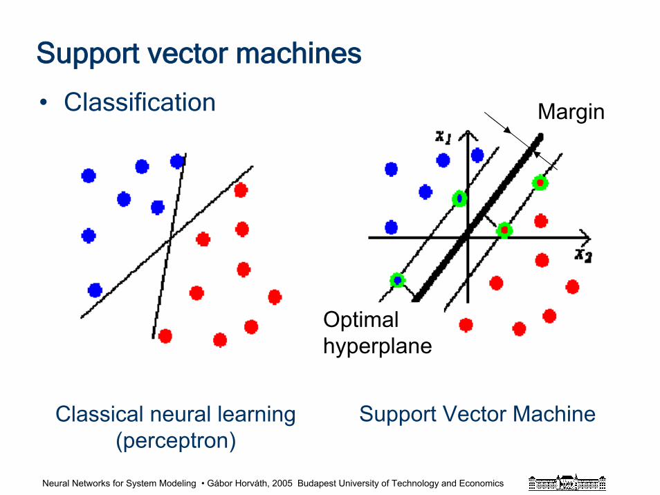
Neural Networks for System Modeling • Gábor Horváth, 2005 Budapest University of Technology and Economics
Classical neural learning(perceptron)
Support Vector Machine
Support vector machines
Optimal hyperplane
• Classification Margin
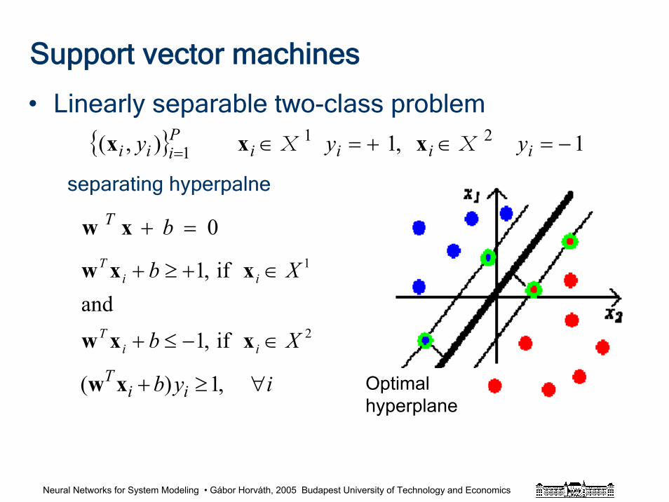
Neural Networks for System Modeling • Gábor Horváth, 2005 Budapest University of Technology and Economics
Support vector machines
• Linearly separable two-class problem
separating hyperpalne
Piii y 1),( =x 1,1 21 −=∈+=∈ iiii yy XX xx
0=+ bT xw
2
1
if,1
and if,1
Xb
Xb
iiT
iiT
∈−≤+
∈+≥+
xxw
xxw
iyb iiT ∀≥+ ,1)( xw Optimal
hyperplane
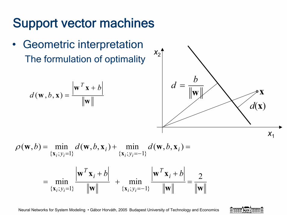
Neural Networks for System Modeling • Gábor Horváth, 2005 Budapest University of Technology and Economics
Support vector machines
ww
xw
w
xw
xwxww
xx
xx
2minmin
),,(min),,(min),(
1;1;
1;1;
=+
++
=
=+=
−==
−==
bb
bdbdb
iT
y
iT
y
iy
iy
iiii
iiiiρ
w
xwxw
bbd
T +=),,( x
d(x)wbd =
x1
x2• Geometric interpretation
The formulation of optimality
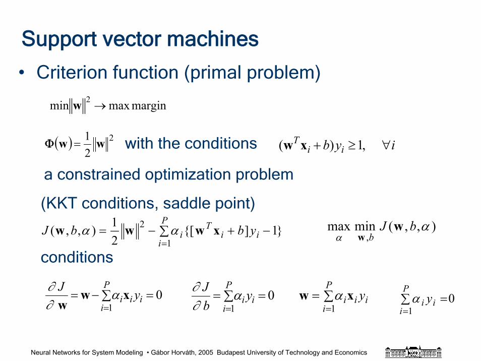
Neural Networks for System Modeling • Gábor Horváth, 2005 Budapest University of Technology and Economics
Support vector machines
• Criterion function (primal problem)
with the conditions
a constrained optimization problem
(KKT conditions, saddle point)
conditions
( ) 2
21 ww =Φ
∑ −+−==
P
iii
Ti ybbJ
1
2 1][21),,( xwww αα
01
=∑−==
iiP
ii yJ xw
wα
∂∂
∑==
P
iiii y
1xw α0
1=∑=
=i
P
ii yb
J α∂∂
01
∑ ==
P
iii yα
),,(minmax,
αα
bJb
ww
iyb iiT ∀≥+ ,1)( xw
marginmaxmin 2 →w
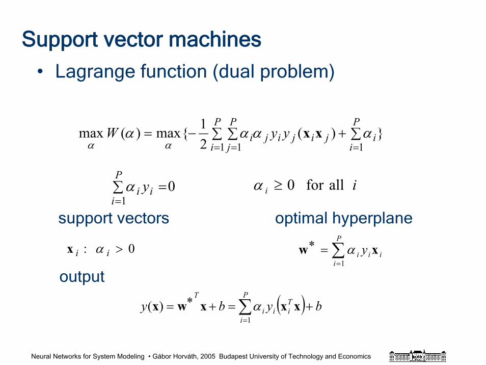
Neural Networks for System Modeling • Gábor Horváth, 2005 Budapest University of Technology and Economics
Support vector machines
• Lagrange function (dual problem)
support vectors optimal hyperplane
output
)(21max)(max
11 1∑+∑ ∑−=== =
P
ii
P
i
P
jjijiji yyW αααα
ααxx
0: >ii αx ∑=
=∗ P
iiii y
1xw α
( ) byby Tii
P
ii
T+=+∗= ∑
=
xxxwx1
)( α
01
∑ ==
P
iii yα allfor 0 ii ≥α
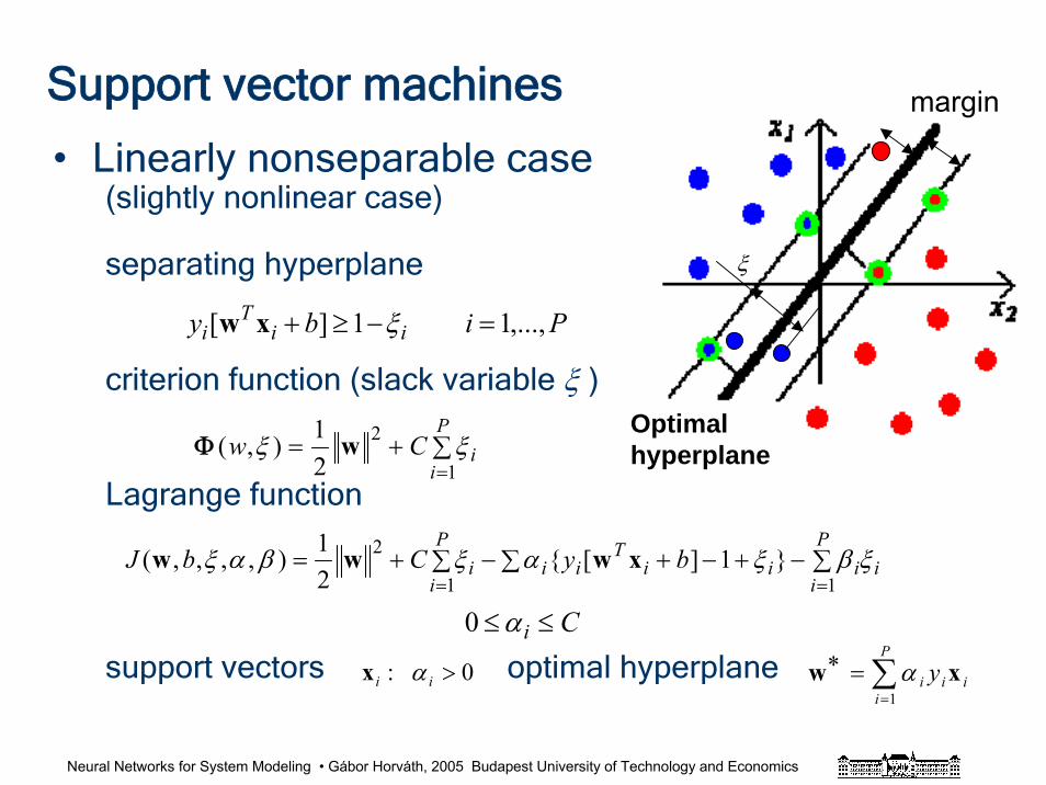
Neural Networks for System Modeling • Gábor Horváth, 2005 Budapest University of Technology and Economics
Support vector machines
• Linearly nonseparable case(slightly nonlinear case)
separating hyperplane
criterion function (slack variable ξ )
Lagrange function
support vectors optimal hyperplane
Piby iiT
i ,...,11][ =−≥+ ξxw
∑+==
P
iiCw
1
2
21),( ξξ wΦ
∑−∑ +−+−∑+===
P
iiiii
Tii
P
ii byCbJ
11
2 1][21),,,,( ξβξαξβαξ xwww
Ci ≤≤ α0
0: >ii αx ∑=
=∗ P
iiii y
1xw α
Optimal hyperplane
margin
ξ
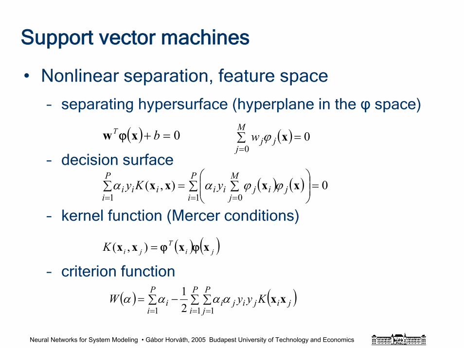
Neural Networks for System Modeling • Gábor Horváth, 2005 Budapest University of Technology and Economics
Support vector machines
• Nonlinear separation, feature space
– separating hypersurface (hyperplane in the φ space)
– decision surface
– kernel function (Mercer conditions)
– criterion function
( ) 0=+ bT xw ϕ
( ) ( ) 0),(1 01
=∑ ⎟⎟⎠
⎞⎜⎜⎝
⎛∑=∑
= ==
P
i
M
jjijiii
P
iii yKy xxxx ϕϕαα
( ) ( )jiT
jiK xxxx ϕϕ=),(
( ) 00
=∑=
M
jjjw xϕ
( ) ( )∑ ∑ ∑−== = =
P
i
P
i
P
jjijijii KyyW
1 1 121 xxαααα
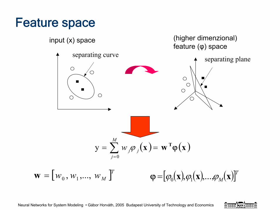
Neural Networks for System Modeling • Gábor Horváth, 2005 Budapest University of Technology and Economics
[ ]TMwww ,...,, 10=w ( ) ( ) ( )[ ]TM xxx ϕϕϕ ,...,, 10=ϕ
( ) ( )xwx Tϕ== ∑=
j
M
jjw ϕ
0
y
separating plane
Feature spaceinput (x) space (higher dimenzional)
feature (φ) spaceseparating curve
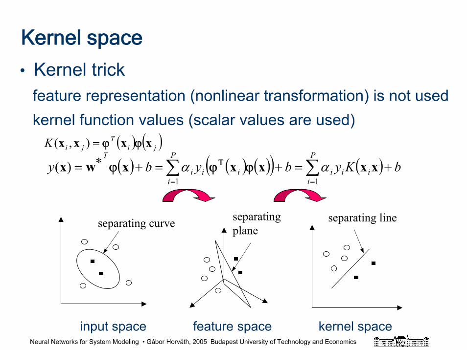
Neural Networks for System Modeling • Gábor Horváth, 2005 Budapest University of Technology and Economics
Kernel space
( ) ( ) ( )( ) ( ) bKybyby ii
P
iiii
P
ii
T+=+=+∗= ∑∑
==
xxxxxwx11
)( αα ϕϕϕ Τ
( ) ( )jiT
jiK xxxx ϕϕ=),(
• Kernel trickfeature representation (nonlinear transformation) is not usedkernel function values (scalar values are used)
separating curve separating plane
separating line
input space feature space kernel space
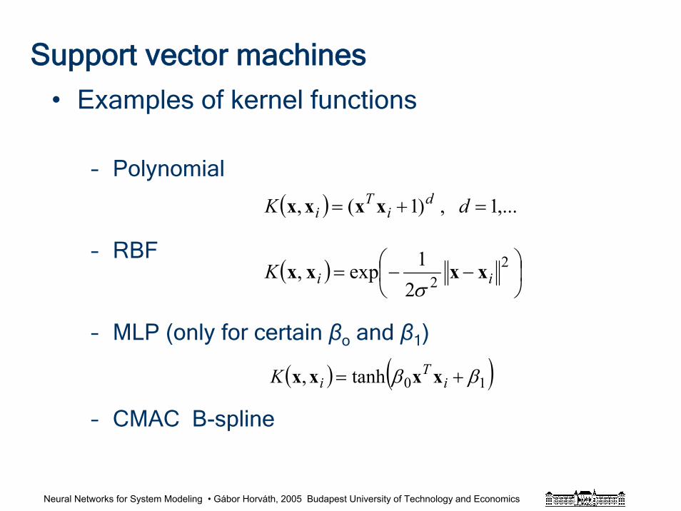
Neural Networks for System Modeling • Gábor Horváth, 2005 Budapest University of Technology and Economics
Support vector machines
• Examples of kernel functions
– Polynomial
– RBF
– MLP (only for certain βo and β1)
– CMAC B-spline
( ) ,...1,)1(, =+= dK di
Ti xxxx
( ) ⎟⎠⎞
⎜⎝⎛ −−= 2
221exp, iiK xxxxσ
( ) ( )10tanh, ββ += iT
iK xxxx
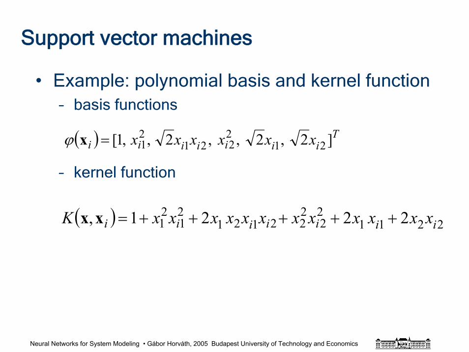
Neural Networks for System Modeling • Gábor Horváth, 2005 Budapest University of Technology and Economics
Support vector machines
• Example: polynomial basis and kernel function– basis functions
– kernel function
( ) 221122
222121
21
21 2221, iiiiiii xxxxxxxxxxxxK +++++=xx
( ) Tiiiiiii xxxxxx ]2,2,,2,,1[ 21
2221
21=xϕ
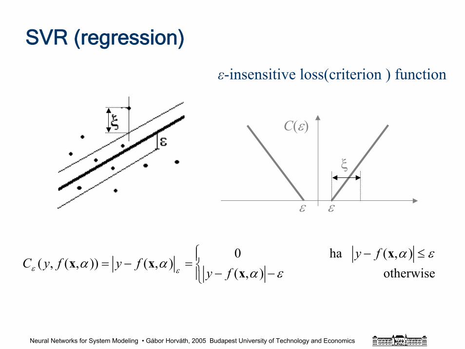
Neural Networks for System Modeling • Gábor Horváth, 2005 Budapest University of Technology and Economics
SVR (regression)
⎪⎩
⎪⎨⎧
−−≤−
=−=otherwise),(
),( ha0),()),(,(
εαεα
ααεε x
xxx
fyfy
fyfyC
εε
C(ε)
ξ
ε-insensitive loss(criterion ) function
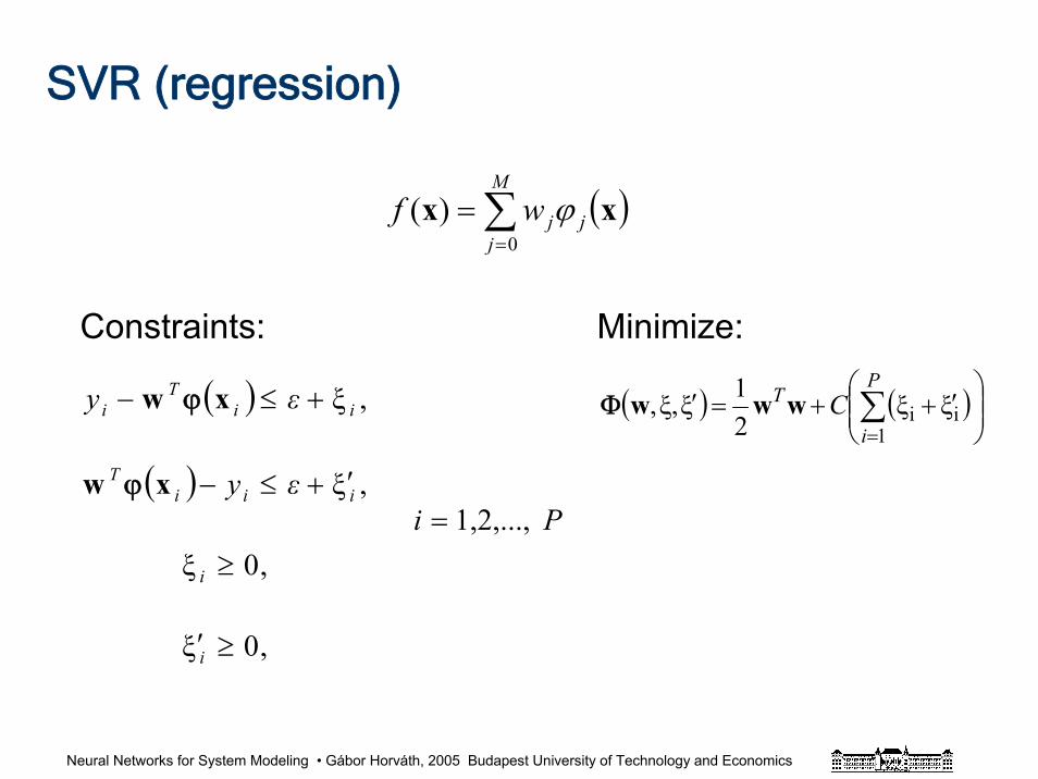
Neural Networks for System Modeling • Gábor Horváth, 2005 Budapest University of Technology and Economics
SVR (regression)
( )
( )Pi
εy
εy
i
i
iiiT
iiT
i
1,2,...,
,0ξ
,0ξ
,ξ
,ξ
=
≥′
≥
′+≤−
+≤−
xw
xw
ϕ
ϕ ( ) ( )⎟⎟⎠
⎞⎜⎜⎝
⎛′++=′ ∑
=
P
i
T C1
ii ξξ21ξξ,, wwwΦ
Constraints: Minimize:
( )∑=
=M
jjjwf
0)( xx ϕ
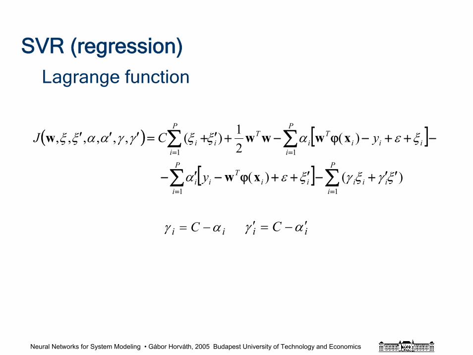
Neural Networks for System Modeling • Gábor Horváth, 2005 Budapest University of Technology and Economics
SVR (regression)
Lagrange function
( ) [ ]
[ ] )()
)21)(,,,,,,
11
11
ξγξγξεα
ξεαξξγγααξξ
′′+−′++ϕ−′−
−++−ϕ−+′+=′′′
∑∑
∑∑
==
==
ii
P
iiii
Ti
P
ii
iiiT
P
ii
Ti
P
ii
y
yCJ
xw
xwwww
(
(
ii C αγ −= ii C αγ ′−=′
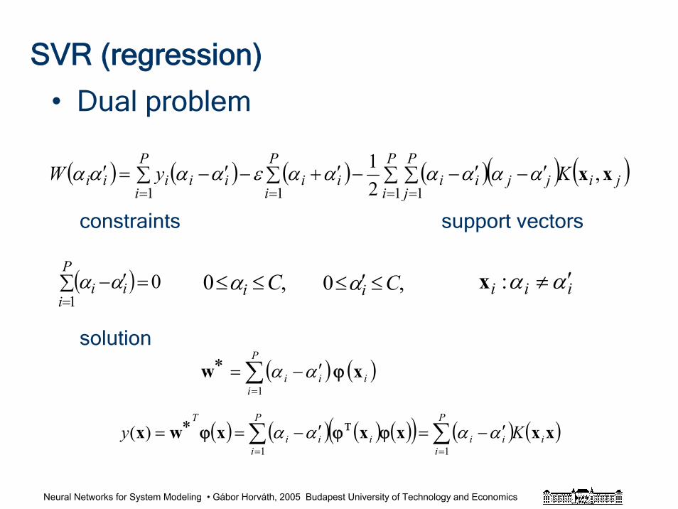
Neural Networks for System Modeling • Gábor Horváth, 2005 Budapest University of Technology and Economics
• Dual problem
SVR (regression)
( ) ( ) ( ) ( )( ) ( )jiP
i
P
jjjii
P
iii
P
iiiiii KyW xx ,
21
1 111∑ ∑ ′−′−−∑ ′+−∑ ′−=′= ===
ααααααεαααα
constraints support vectors
( ) 01
=∑ ′−=
P
iii αα ,0 Ci ≤≤α ,0 Ci ≤′≤α iii αα ′≠:x
( ) ( )i
P
iii xw ϕ∑
=
′−=∗1
αα
( ) ( ) ( ) ( )( ) ( ) ( )xxxxxwx i
P
iiii
P
iii
TKy ∑∑
==
′−=′−=∗=11
)( αααα ϕϕϕ Τ
solution
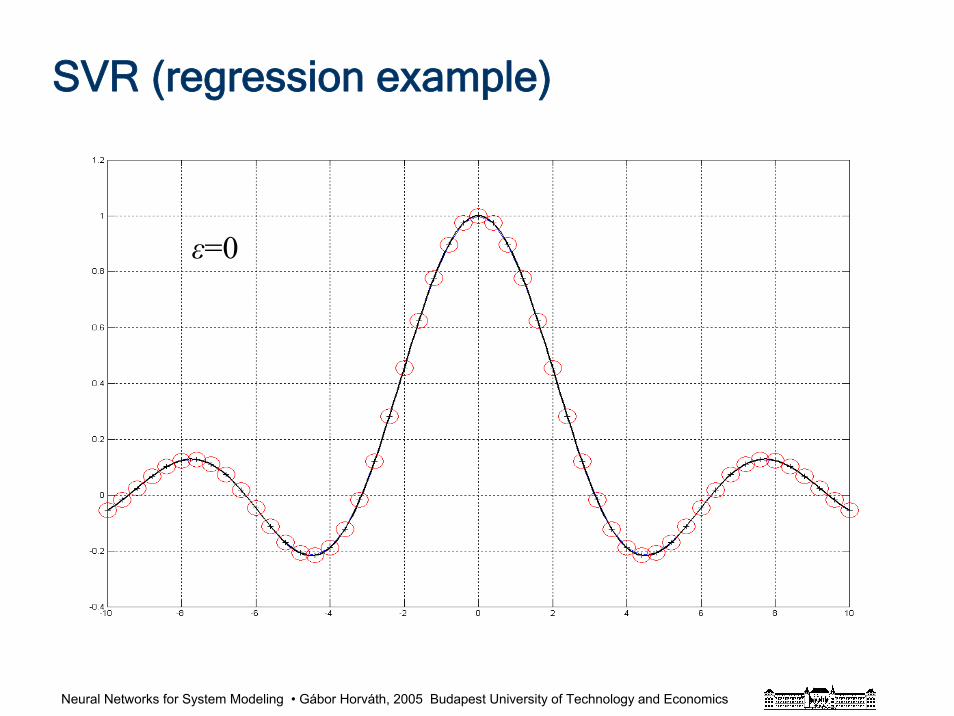
Neural Networks for System Modeling • Gábor Horváth, 2005 Budapest University of Technology and Economics
SVR (regression example)
ε=0
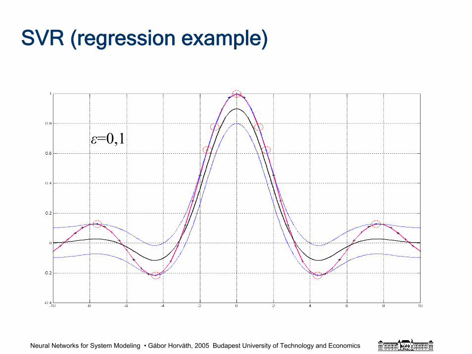
Neural Networks for System Modeling • Gábor Horváth, 2005 Budapest University of Technology and Economics
SVR (regression example)
ε=0,1
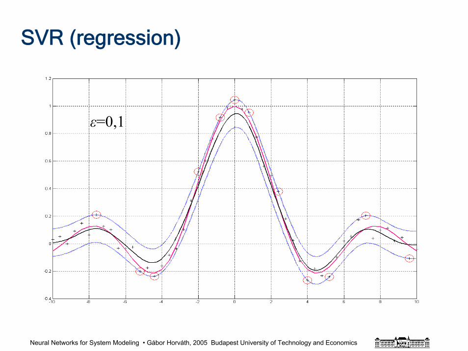
Neural Networks for System Modeling • Gábor Horváth, 2005 Budapest University of Technology and Economics
SVR (regression)
ε=0,1
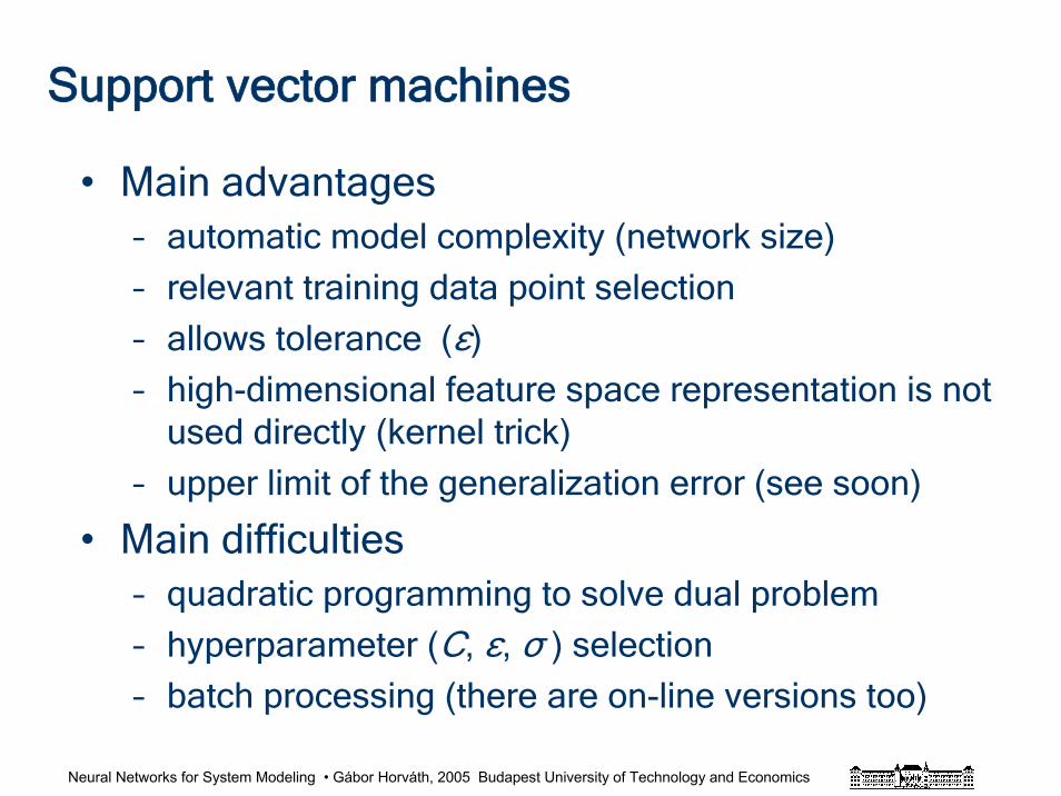
Neural Networks for System Modeling • Gábor Horváth, 2005 Budapest University of Technology and Economics
Support vector machines
• Main advantages– automatic model complexity (network size)
– relevant training data point selection
– allows tolerance (ε)
– high-dimensional feature space representation is not used directly (kernel trick)
– upper limit of the generalization error (see soon)
• Main difficulties– quadratic programming to solve dual problem
– hyperparameter (C, ε, σ ) selection
– batch processing (there are on-line versions too)
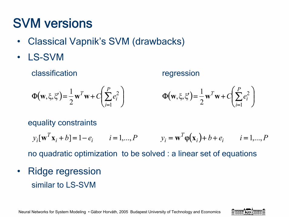
Neural Networks for System Modeling • Gábor Horváth, 2005 Budapest University of Technology and Economics
SVM versions• Classical Vapnik’s SVM (drawbacks)
• LS-SVM
classification regression
equality constraints
no quadratic optimization to be solved : a linear set of equations
• Ridge regressionsimilar to LS-SVM
( ) ⎟⎟⎠
⎞⎜⎜⎝
⎛+=′Φ ∑
=
P
ii
T eC1
221ξξ,, www
Pieby iiT
i ,...,11][ =−=+xw
( ) ⎟⎟⎠
⎞⎜⎜⎝
⎛+=′Φ ∑
=
P
ii
T eC1
221ξξ,, www
( ) Pieby iiT
i ,...,1=++ϕ= xw
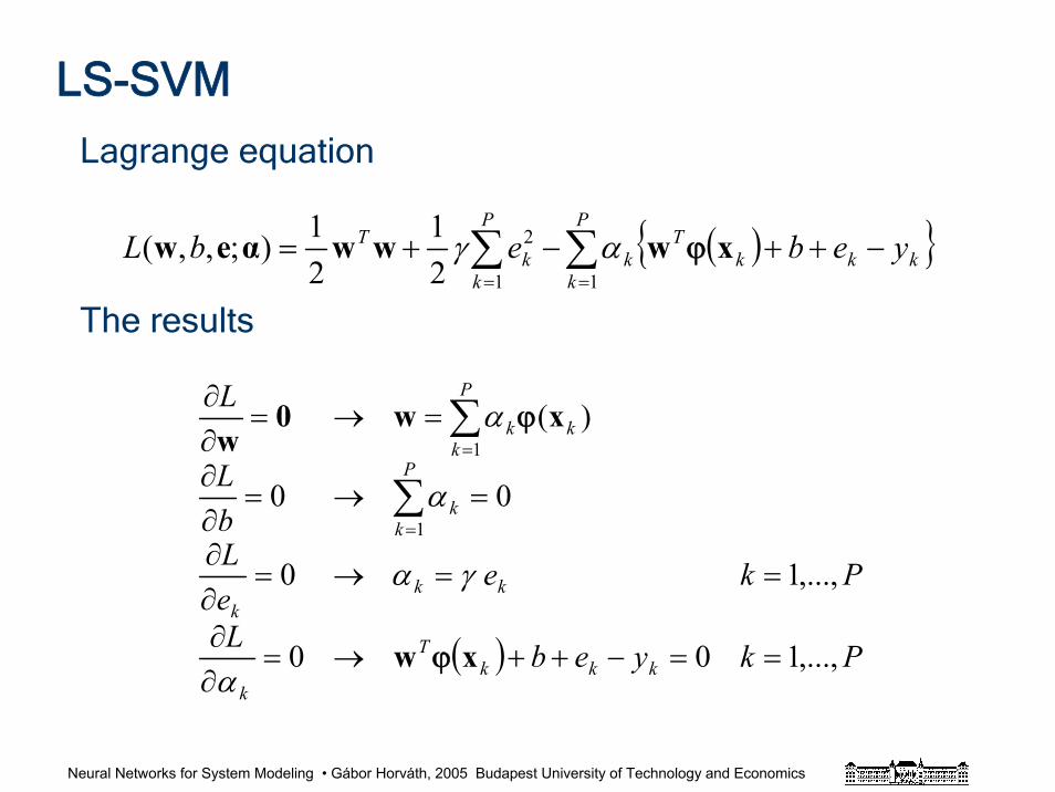
Neural Networks for System Modeling • Gábor Horváth, 2005 Budapest University of Technology and Economics
LS-SVM
Lagrange equation
The results
( ) ∑∑==
−++−+=P
kkkk
Tk
P
kk
T yebebL11
2
21
21);,,( xwwwαew ϕαγ
( ) PkyebL
PkeeLbL
L
kkkT
k
kkk
P
kk
P
kkk
,...,100
,...,1 0
00
)(
1
1
==−++→=∂∂
==→=∂∂
=→=∂∂
=→=∂∂
∑
∑
=
=
xw
xw0w
ϕ
ϕ
α
γα
α
α
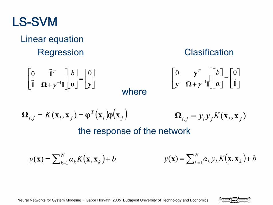
Neural Networks for System Modeling • Gábor Horváth, 2005 Budapest University of Technology and Economics
LS-SVMLinear equation
Regression Clasification
where
the response of the network
⎥⎦
⎤⎢⎣
⎡=⎥
⎦
⎤⎢⎣
⎡
⎥⎥⎦
⎤
⎢⎢⎣
⎡
+ − yαIΩ11 00
1
bT
γr
r
⎥⎦
⎤⎢⎣
⎡=⎥
⎦
⎤⎢⎣
⎡⎥⎦
⎤⎢⎣
⎡
+ − 1αIΩyy
r00
1
bT
γ
),(, jijiji Kyy xxΩ =( ) ( )jiT
jiji K xxxxΩ ϕϕ== ),(,
( )∑ =+= N
k kk bKαy 1 ,)( xxx ( )∑ =+= N
k kkk bKyαy 1 ,)( xxx
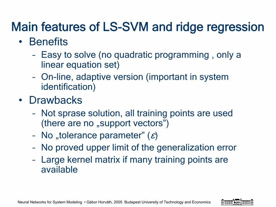
Neural Networks for System Modeling • Gábor Horváth, 2005 Budapest University of Technology and Economics
Main features of LS-SVM and ridge regression• Benefits
– Easy to solve (no quadratic programming , only a linear equation set)
– On-line, adaptive version (important in system identification)
• Drawbacks– Not sprase solution, all training points are used
(there are no „support vectors”)– No „tolerance parameter” (ε)– No proved upper limit of the generalization error– Large kernel matrix if many training points are
available
Neural Networks for System Modeling • Gábor Horváth, 2005 Budapest University of Technology and Economics
Improved LS Kernel machines
• There are sparse versions of the LS-SVM– The training points are ranked and only the most
important ones are used (iterative solution)
– The kernel matrix can be reduced (a tolerance parameter is introduced again)
– Detailes: see the references
• Additional contraints can be used for special applications (see e.g. regularized kernel CMAC)
Neural Networks for System Modeling • Gábor Horváth, 2005 Budapest University of Technology and Economics
• Goal– General goal:
to show that additional constraints can be used in the framework of LS-SVM
here: the additional constraint is a weight-smoothing term
– Special goal:
to show that kernel approach can be used for improving the modelling capability of the CMAC
Kernel CMAC (an example)
Neural Networks for System Modeling • Gábor Horváth, 2005 Budapest University of Technology and Economics
General goal• Introducing new constraints• General LS-SVM problem
Criterion function: two termsweight minimization term + error term
Lagrange functioncriterion function+ Lagrange term
Extensionadding new constraint to the criterion function
Extended Lagrange functionnew criterion function (with the new constraint) + Lagrange term
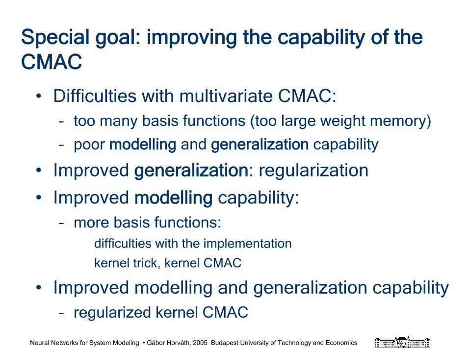
Neural Networks for System Modeling • Gábor Horváth, 2005 Budapest University of Technology and Economics
Special goal: improving the capability of the CMAC
• Difficulties with multivariate CMAC:– too many basis functions (too large weight memory)
– poor modelling and generalization capability
• Improved generalization: regularization
• Improved modelling capability:– more basis functions:
difficulties with the implementation
kernel trick, kernel CMAC
• Improved modelling and generalization capability– regularized kernel CMAC
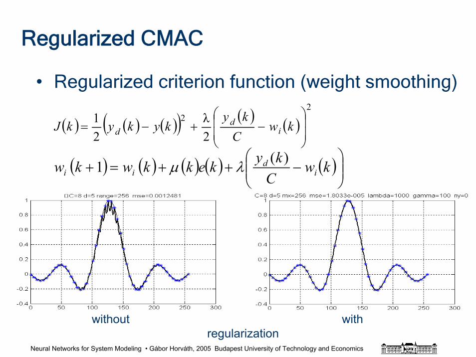
Neural Networks for System Modeling • Gábor Horváth, 2005 Budapest University of Technology and Economics
Regularized CMAC
• Regularized criterion function (weight smoothing)
( ) ( ) ( )( ) ( ) ( )2
2
2λ
21
⎟⎟
⎠
⎞
⎜⎜
⎝
⎛−+−= kw
Cky
kykykJ id
d
( ) ( ) ( ) ( ) ( )⎟⎟⎠
⎞⎜⎜⎝
⎛−++=+ kw
Ckykekkwkw i
dii
)(1 λμ
without withregularization
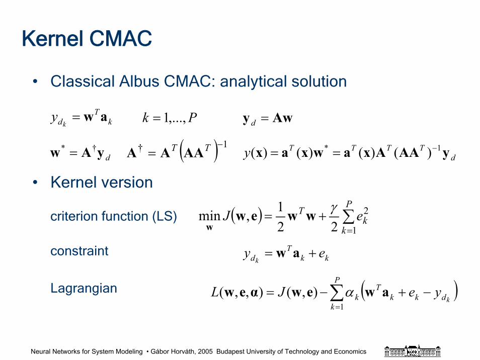
Neural Networks for System Modeling • Gábor Horváth, 2005 Budapest University of Technology and Economics
Kernel CMAC
• Classical Albus CMAC: analytical solution
• Kernel version
criterion function (LS)
constraint
Lagrangian
kT
dky aw=
dyAw †* = ( ) 1† −= TT AAAA d
TTTTy yAAAxawxax 1* )()()()( −==
Awy =d
( ) ∑=
+=P
kk
T eJ1
2
221,min γwwew
w
kkT
d eyk
+= aw
Pk ,...,1=
( )∑=
−+−=P
kdkk
Tk k
yeJL1
),(),,( awewαew α
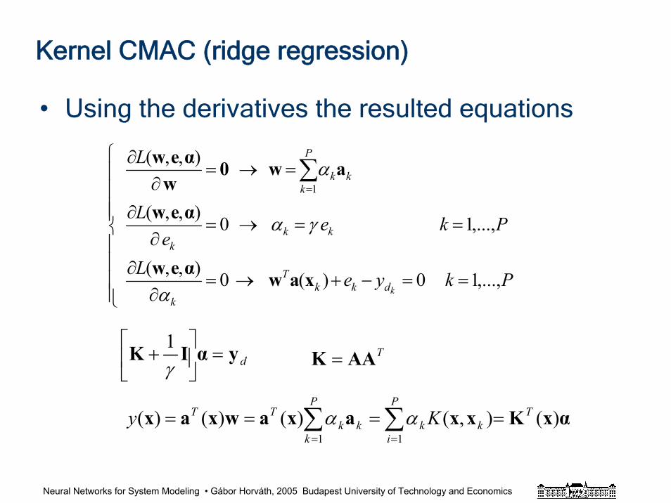
Neural Networks for System Modeling • Gábor Horváth, 2005 Budapest University of Technology and Economics
Kernel CMAC (ridge regression)
• Using the derivatives the resulted equations
⎪⎪⎪⎪
⎩
⎪⎪⎪⎪
⎨
⎧
==−+→=∂
∂
==→=∂
∂
=→=∂
∂ ∑=
PkyeL
Pkee
L
L
kdkkT
k
kkk
P
kkk
,...,1 0)(0),,(
,...,1 0),,(
),,(1
xawαew
αew
aw0wαew
α
γα
α
dyαIK =⎥⎦
⎤⎢⎣
⎡+
γ1
TAAK =
αxKxxaxawxax )(),()()()(11
TP
ikkk
P
kk
TT Ky ==== ∑∑==
αα
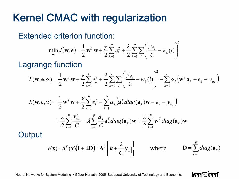
Neural Networks for System Modeling • Gábor Horváth, 2005 Budapest University of Technology and Economics
Kernel CMAC with regularization
( ) ∑∑∑==
⎟⎟⎠
⎞⎜⎜⎝
⎛−++=
P
k ik
dP
kk
T iwCy
eJ k
1
2
1
2 )(222
1,min λγwweww
( )∑∑∑∑===
−+−⎟⎟⎠
⎞⎜⎜⎝
⎛−++=
P
kdkk
Tk
P
k ik
dP
kk
Tk
k yeiwCy
eL11
2
1
2 )(222
1),,( awwwew αλγα
( )
wawwaa
waawwew
)(2
)(2
)(22
1),,(
111
211
2
k
P
k
Tk
TP
k
kP
k
d
P
kdkk
Tk
P
kk
T
diagdiagCd
Cy
yediageL
kk
kk
∑∑∑
∑∑
===
==
+−+
−+−+=
λλλ
αγα
Extended criterion function:
Lagrange function
Output( ) ⎥⎦
⎤⎢⎣⎡ ++= −
dTT
Cy yαADIxax λλ 1)()( ∑
=
=P
kkdiag
1)(aDwhere
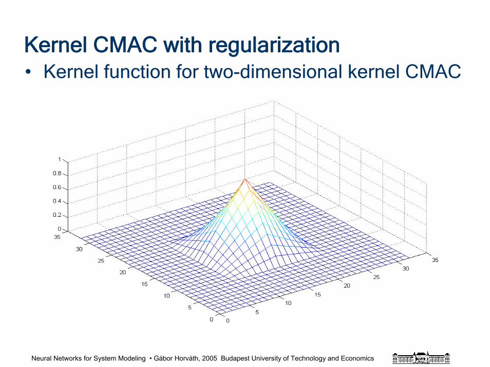
Neural Networks for System Modeling • Gábor Horváth, 2005 Budapest University of Technology and Economics
• Kernel function for two-dimensional kernel CMACKernel CMAC with regularization
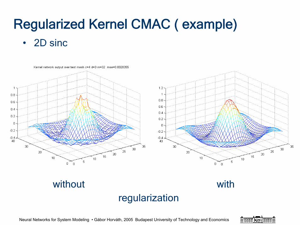
Neural Networks for System Modeling • Gábor Horváth, 2005 Budapest University of Technology and Economics
Regularized Kernel CMAC ( example)• 2D sinc
without with regularization
Neural Networks for System Modeling • Gábor Horváth, 2005 Budapest University of Technology and Economics
References and further readingsHaykin, S.: "Neural Networks. A Comprehensive Foundation" Prentice Hall, N. J.1999.
Saunders, C.- Gammerman, A. and Vovk, V. "Ridge Regression Learning Algorithm in Dual Variables. Machine Learning", Proc. of the Fifteenth International Conference on Machine Learning, pp. 515-521, 1998.
Schölkopf, B. and Smola, P. "Learning with Kernels. Support Vector Machines, Regularization, Optimization and Beyond" MIT Press, Cambridge, MA, 2002.
Suykens, J.A.K., Van Gestel, T, De Brabanter, J., De Moor, B. and Vandewalle, J. "Least Squares Support Vector Machines", World Scientific, Singapore, 2002.
Vapnik, V. "Statistical Learning Theory", Wiley, New York, 1995.
Horváth, G. "CMAC: Reconsidering an Old Neural Network" Proc. of the Intelligent Control Systems and Signal Processing, ICONS 2003, Faro, Portugal. pp. 173-178, 2003.
Horváth, G. "Kernel CMAC with Improved Capability" Proc. of the International Joint Conference on Neural Networks, IJCNN’2004, Budapest, Hungary. 2004.
Lane, S.H. - Handelman, D.A. and Gelfand, J.J "Theory and Development of Higher-Order CMAC Neural Networks", IEEE Control Systems, Vol. Apr. pp. 23-30, 1992.
Szabó, T. and Horváth, G. "Improving the Generalization Capability of the Binary CMAC” Proc. of the International Joint Conference on Neural Networks, IJCNN’2000. Como, Italy, Vol. 3, pp. 85-90, 2000.
Neural Networks for System Modeling • Gábor Horváth, 2005 Budapest University of Technology and Economics
Statistical learning theory
• Main question: how can the quality of a learning machine be estimated
• Generalization measure based on the empirical risk (error).
• Empirical risk: the error determined in the training points
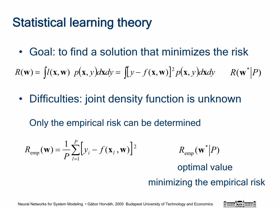
Neural Networks for System Modeling • Gábor Horváth, 2005 Budapest University of Technology and Economics
Statistical learning theory
• Goal: to find a solution that minimizes the risk
• Difficulties: joint density function is unknown
Only the empirical risk can be determined
optimal value
minimizing the empirical risk
( ) [ ] ( ) dydypfydydyplR xxwxxxwxw ,),(,),()( 2∫∫ −==
[ ]∑=
−=P
lli fy
PR
1
2emp ),(1)( wxw )( *
emp PR w
)( * PR w
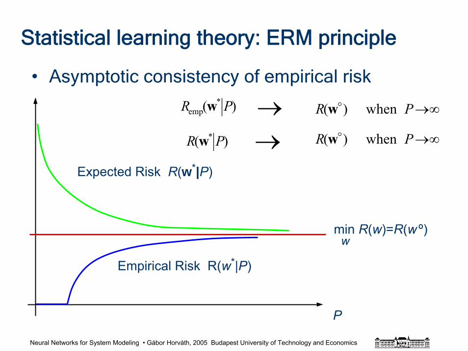
Neural Networks for System Modeling • Gábor Horváth, 2005 Budapest University of Technology and Economics
Statistical learning theory: ERM principle
• Asymptotic consistency of empirical risk
P
min R(w)=R(w º)w
Expected Risk R(w*|P)
Empirical Risk R(w*|P)
)( * PR w
)( *emp PR w →
→∞→PR when )( ow
∞→PR when )( ow
Neural Networks for System Modeling • Gábor Horváth, 2005 Budapest University of Technology and Economics
Statistical learning theory
• Condition of consistency of the ERM principleNecessarry and sufficient condition: finite VC dimension
Also: this is a sufficient condition of fast convergence
• VC (Vapnik-Chervonenkis) dimension:A set of function has VC dimension h if there exist hsamples that can be shattered (can be separated into two classes in all possible ways: all 2h possible ways) by this set of functions but there do not exist h +1 samples that can be shattered by the same set of functions.
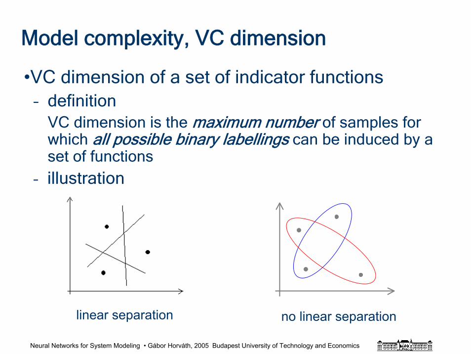
Neural Networks for System Modeling • Gábor Horváth, 2005 Budapest University of Technology and Economics
Model complexity, VC dimension
•VC dimension of a set of indicator functions– definition
VC dimension is the maximum number of samples forwhich all possible binary labellings can be induced by aset of functions
– illustration
linear separation no linear separation
Neural Networks for System Modeling • Gábor Horváth, 2005 Budapest University of Technology and Economics
VC dimension
• Based on VC dimension upper bounds of the risk can be obtained
• Calculating the VC dimension– general case: rather difficult
e.g for MLP VC-dimension can be infinite
– special cases: e.g. linear function set
• VC dimension of a set of linear functions (linear separating task)
h =N +1 (N : input space dimension)
An important statement: It can be proved that the VC dimension can be less than N +1
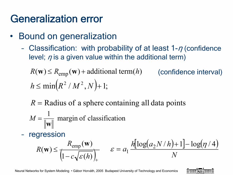
Neural Networks for System Modeling • Gábor Horváth, 2005 Budapest University of Technology and Economics
Generalization error
• Bound on generalization– Classification: with probability of at least 1-η (confidence
level; η is a given value within the additional term)
– regression
)( termadditional)()( emp hRR +≤ ww
( ) ;1,/min 22 +≤ NMRh
points data all containing sphere a of Radius=R
tionclassifica ofmargin 1w
=M
(confidence interval)
( )+−≤
)(1
)()( emp
hc
RR
ε
ww
( )[ ] ( )N
hNaha 4/log1/log 21
ηε
−+=
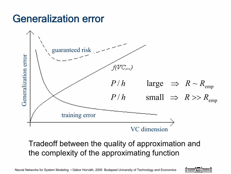
Neural Networks for System Modeling • Gábor Horváth, 2005 Budapest University of Technology and Economics
Generalization error
guaranteed risk
training error
VC dimension
Gen
eral
iza t
ion
erro
r
Tradeoff between the quality of approximation and the complexity of the approximating function
emp
emp
small /
~ large/
RRhP
RRhP
>>⇒
⇒
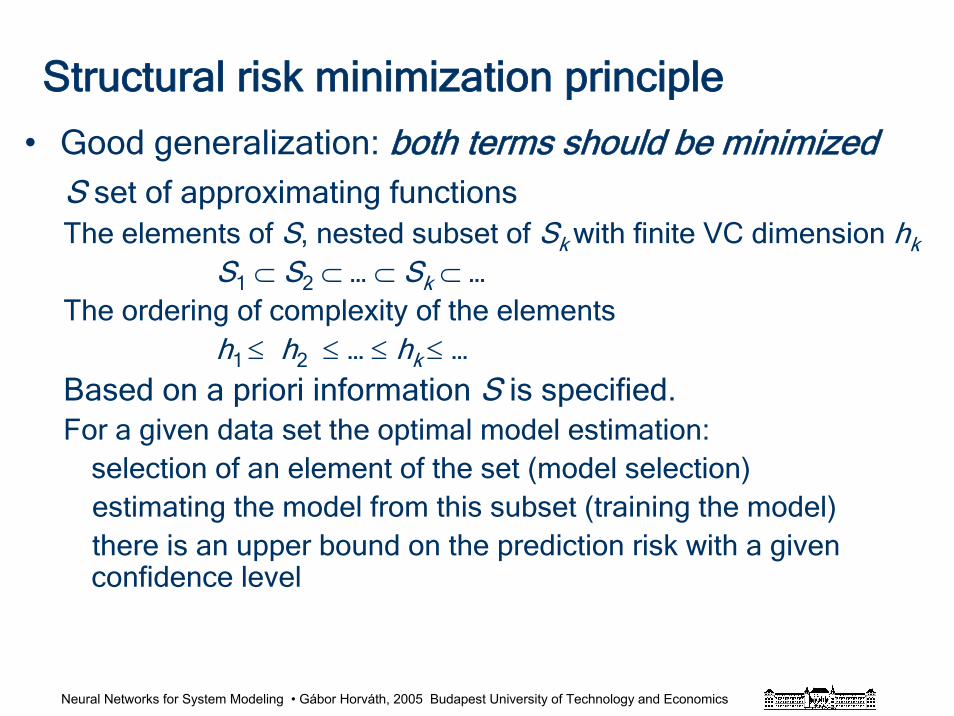
Neural Networks for System Modeling • Gábor Horváth, 2005 Budapest University of Technology and Economics
Structural risk minimization principle
• Good generalization: both terms should be minimizedS set of approximating functionsThe elements of S, nested subset of Sk with finite VC dimension hk
S1 ⊂ S2 ⊂ … ⊂ Sk ⊂ …The ordering of complexity of the elements
h1 ≤ h2 ≤ … ≤ hk ≤ …Based on a priori information S is specified.For a given data set the optimal model estimation:
selection of an element of the set (model selection)estimating the model from this subset (training the model)there is an upper bound on the prediction risk with a givenconfidence level
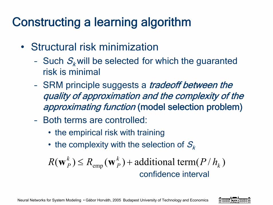
Neural Networks for System Modeling • Gábor Horváth, 2005 Budapest University of Technology and Economics
Constructing a learning algorithm
• Structural risk minimization– Such Sk will be selected for which the guaranted
risk is minimal
– SRM principle suggests a tradeoff between the quality of approximation and the complexity of the approximating function (model selection problem)
– Both terms are controlled:• the empirical risk with training
• the complexity with the selection of Sk
)/( termadditional)()( emp kkP
kP hPRR +≤ ww
confidence interval
Neural Networks for System Modeling • Gábor Horváth, 2005 Budapest University of Technology and Economics
SVM
• Support vector machines are such a learning machines that minimize the length of the weight vector
• They minimize the VC dimension. The upper bounds are valid for SVMs.
• For SVMs not only the structure (the size of the network) can be determined, but an estimate of its generalization error can be obtained.
Neural Networks for System Modeling • Gábor Horváth, 2005 Budapest University of Technology and Economics
References and further readingsHaykin, S.: "Neural Networks. A Comprehensive Foundation" Prentice Hall, N.
J.1999.
Vapnik, V. "Statistical Learning Theory", Wiley, New York, 1998.
Cherkassky, V., Mulier, F. „Learning from Data, Concepts, Theory, and Methods”, John Wiley and Sons,1998.

Neural Networks for System Modeling • Gábor Horváth, 2005 Budapest University of Technology and Economics
Modular network architectures
Neural Networks for System Modeling • Gábor Horváth, 2005 Budapest University of Technology and Economics
Modular solution
• A set of networks: competition/cooperation
– all networks solve the same problem (competition/cooperation)
– the whole problem is decomposed: the different networks solve
different part of the whole problem (cooperation)
• Ensemble of networks
– linear combination of networks
• Mixture of experts
– using the same paradigm (e.g. neural networks)
– using different paradigms (e.g. neural networks + symbolic
systems, neural networks + fuzzy systems)
Neural Networks for System Modeling • Gábor Horváth, 2005 Budapest University of Technology and Economics
Cooperative networks
Ensemble of cooperating networks
(classification/regression)
• The motivation
– Heuristic explanation
• Different experts together can solve a problem better
• Complementary knowledge
– Mathematical justification
• Accurate and diverse modules
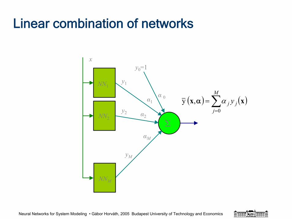
Neural Networks for System Modeling • Gábor Horváth, 2005 Budapest University of Technology and Economics
Linear combination of networks
NNM
NN1
NN2
α1
α2
αM
Σ
y1
y2
yM
x
NNM
α 0
y0=1
( ) ( )xx j
M
jj y∑
=
=0
,y αα
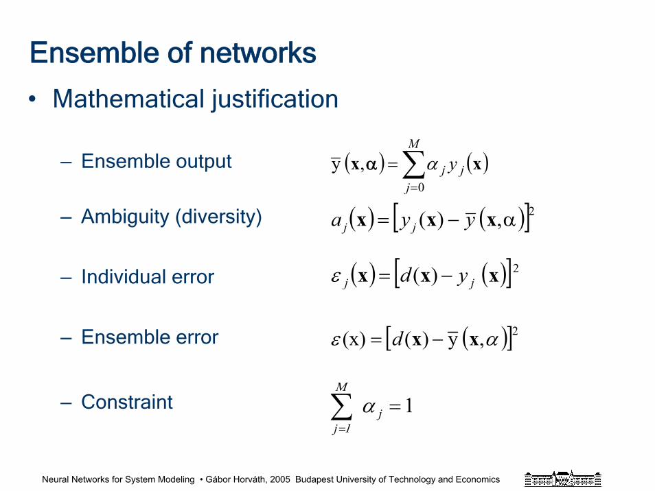
Neural Networks for System Modeling • Gábor Horváth, 2005 Budapest University of Technology and Economics
Ensemble of networks
• Mathematical justification
– Ensemble output
– Ambiguity (diversity)
– Individual error
– Ensemble error
– Constraint
( ) ( )xx j
M
jj y∑
=
=0
,y αα
( )[ ]2,y)((x) αε xx −= d
( ) ( )[ ]2)( xxx jj yd −=ε
( ) ( )[ ]2,)( α−= xxx yya jj
1=∑=
jj
αΜ
1
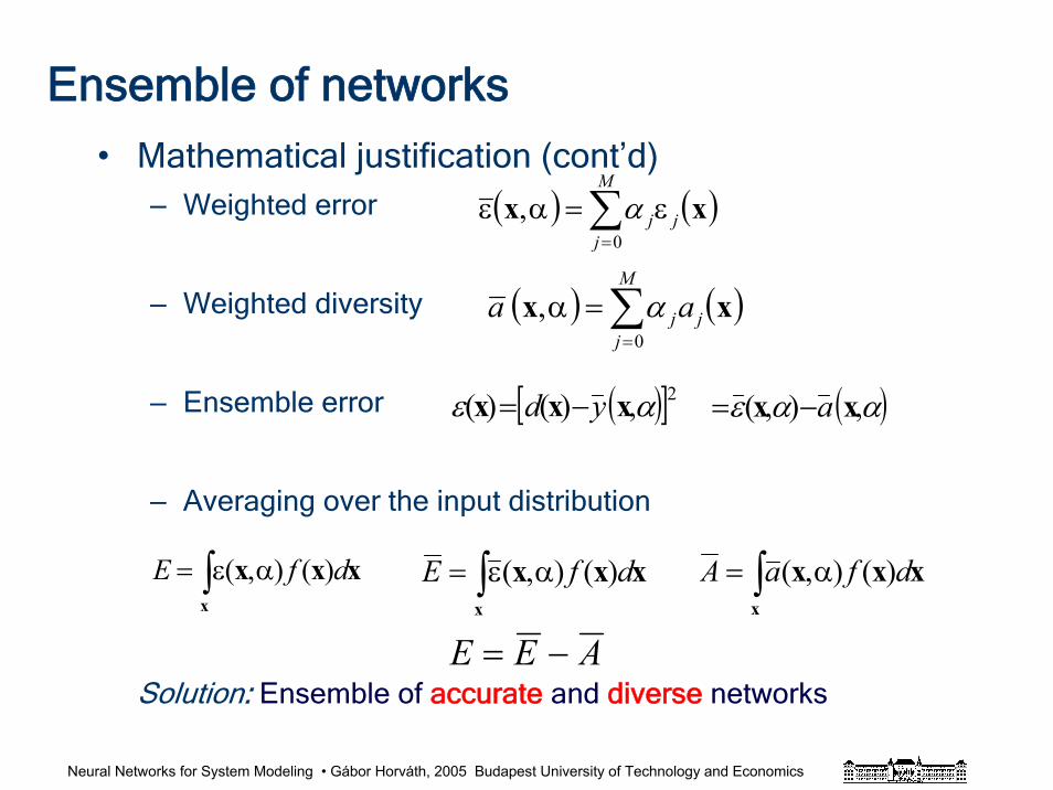
Neural Networks for System Modeling • Gábor Horváth, 2005 Budapest University of Technology and Economics
Ensemble of networks
• Mathematical justification (cont’d)– Weighted error
– Weighted diversity
– Ensemble error
– Averaging over the input distribution
Solution: Ensemble of accurate and diverse networks
( ) ( )xx j
M
jjaa ∑
=
=α0
, α
( ) ( )xx j
M
jjε=αε ∑
=0, α
( )[ ]2,)()( αε xxx yd −= ( )ααε ,),( xx a−=
∫ αε=x
xxx dfE )(),( ∫ αε=x
xxx dfE )(),( ∫ α=x
xxx dfaA )(),(
AEE −=
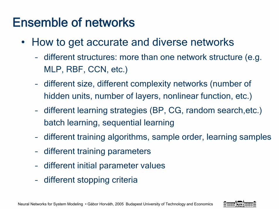
Neural Networks for System Modeling • Gábor Horváth, 2005 Budapest University of Technology and Economics
Ensemble of networks
• How to get accurate and diverse networks– different structures: more than one network structure (e.g.
MLP, RBF, CCN, etc.)
– different size, different complexity networks (number of
hidden units, number of layers, nonlinear function, etc.)
– different learning strategies (BP, CG, random search,etc.)
batch learning, sequential learning
– different training algorithms, sample order, learning samples
– different training parameters
– different initial parameter values
– different stopping criteria
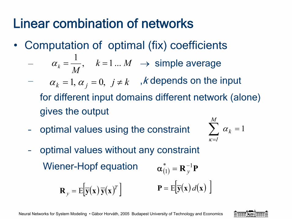
Neural Networks for System Modeling • Gábor Horváth, 2005 Budapest University of Technology and Economics
Linear combination of networks
• Computation of optimal (fix) coefficients
– → simple average
– ,k depends on the input
for different input domains different network (alone)
gives the output
– optimal values using the constraint
– optimal values without any constraint
Wiener-Hopf equation
MkMk ...1,1
==α
kjjk ≠== ,0,1 αα
( ) PR 1*1
−= yα
( ) ( )[ ]Ty xyxyR E=
1=∑=
kαΜ
1κ
( ) ( )[ ]xxyP dE=
Neural Networks for System Modeling • Gábor Horváth, 2005 Budapest University of Technology and Economics
References and further readingsHaykin, S.: "Neural Networks. A Comprehensive Foundation" Prentice Hall, N.
J.1999.
Hashem, S. “Optimal Linear Combination of Neural Networks” Neural Networks, Vol. 10. No. 4. pp. 599-614, 1997.
Krogh, A, Vedelsby, J.: “Neural Network Ensembles Cross Validation and Active Learning” InTesauro, G, Touretzky, D, Leen, T. Advances in Neural Information Processing Systems, 7. Cambridge, MA. MIT Press pp. 231-238.
Gasser Auda and Mohamed Kamel: „Modular Neural Networks: A survey” Pattern Analysis andíMachine Intelligence Lab. Systems Design Engineering Department, University of Waterloo, Canada.
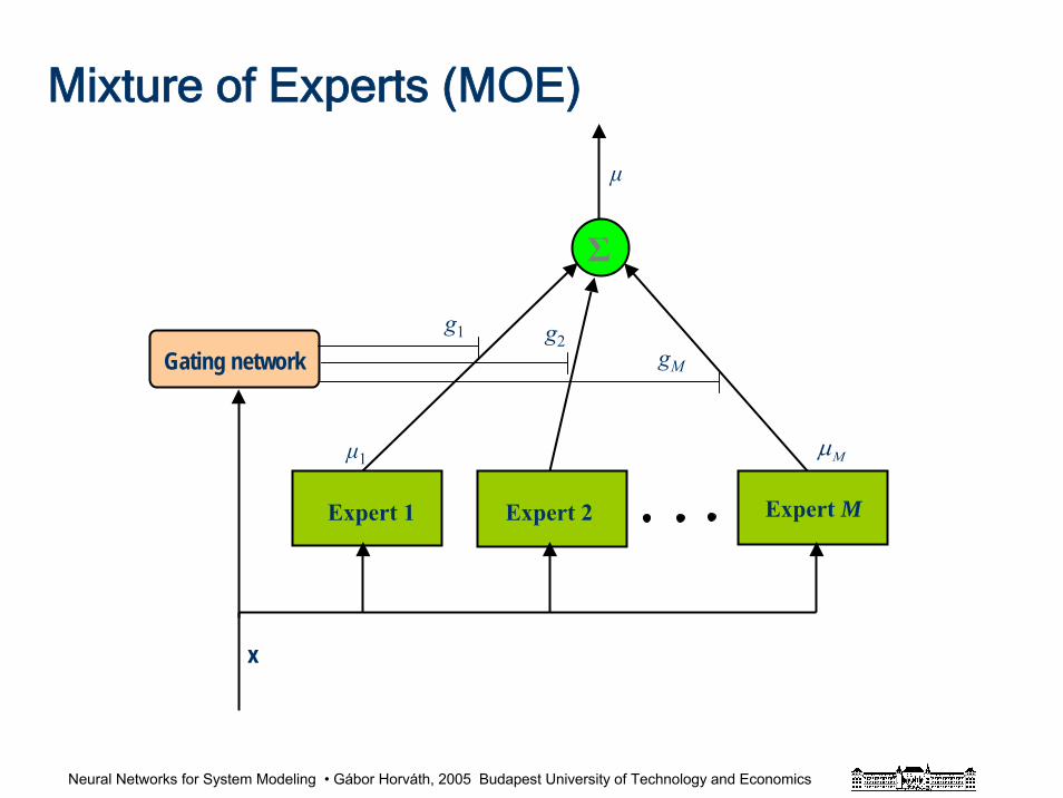
Neural Networks for System Modeling • Gábor Horváth, 2005 Budapest University of Technology and Economics
Mixture of Experts (MOE)
Expert 2Expert 1
Gating network
μ1
μ
g1 g2
x
Expert M
gM
Σ
μΜ
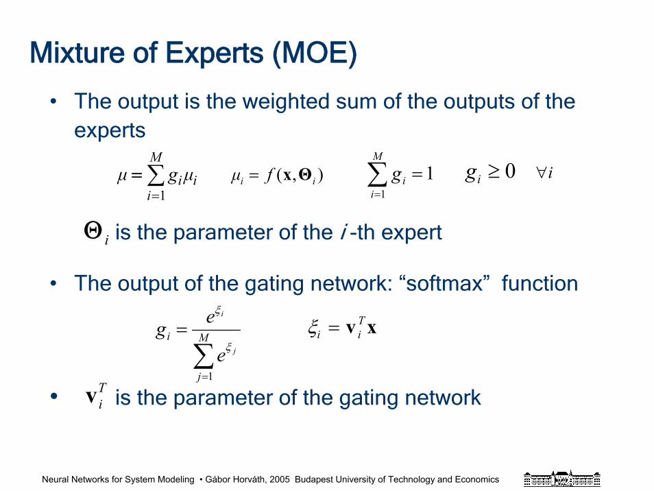
Neural Networks for System Modeling • Gábor Horváth, 2005 Budapest University of Technology and Economics
Mixture of Experts (MOE)
• The output is the weighted sum of the outputs of the experts
is the parameter of the i -th expert
• The output of the gating network: “softmax” function
• is the parameter of the gating network
∑=
= M
j
ij
i
e
eg
1
ξ
ξ
ξi iT= v x
i
M
iiμgμ ∑
=1= 1
1=∑
=
M
iig 0≥ig i∀),( ii fμ Θx=
iΘ
Tiv
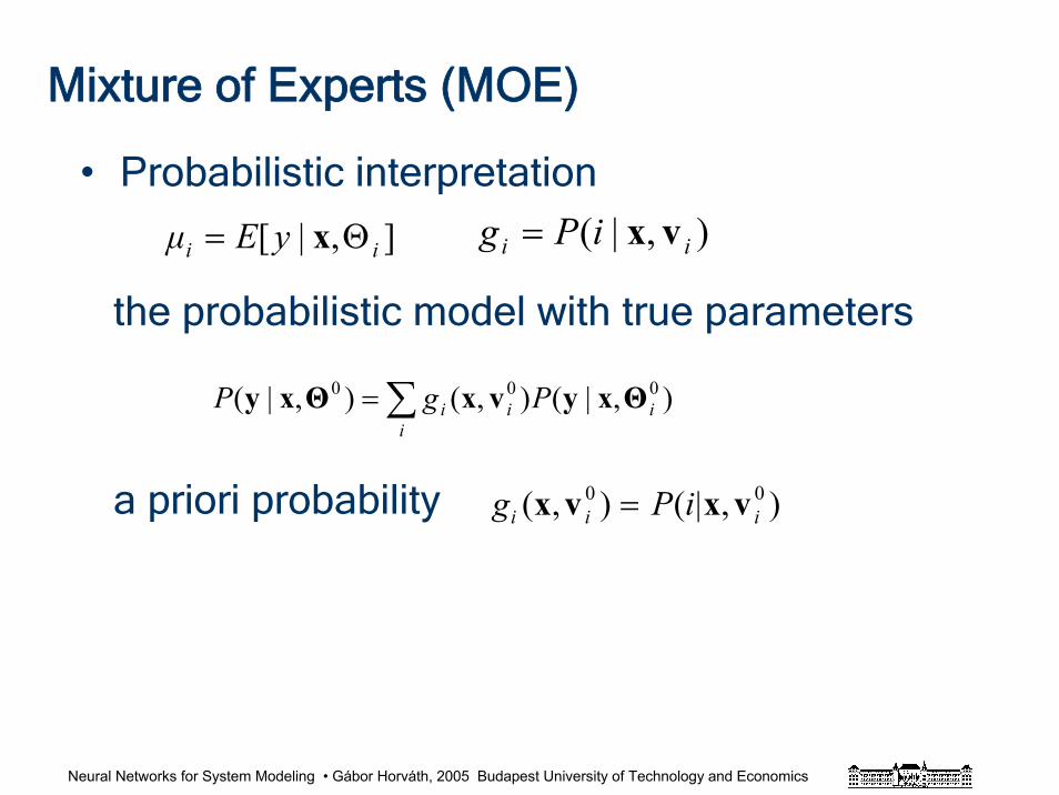
Neural Networks for System Modeling • Gábor Horváth, 2005 Budapest University of Technology and Economics
Mixture of Experts (MOE)
• Probabilistic interpretation
the probabilistic model with true parameters
a priori probability
],|[ ii yEμ Θ= x ),|( ii iPg vx=
∑=i
iii PgP ),|(),(),|( 000 ΘxyvxΘxy
g P ii i i( , ) ( | , )x v x v0 0=
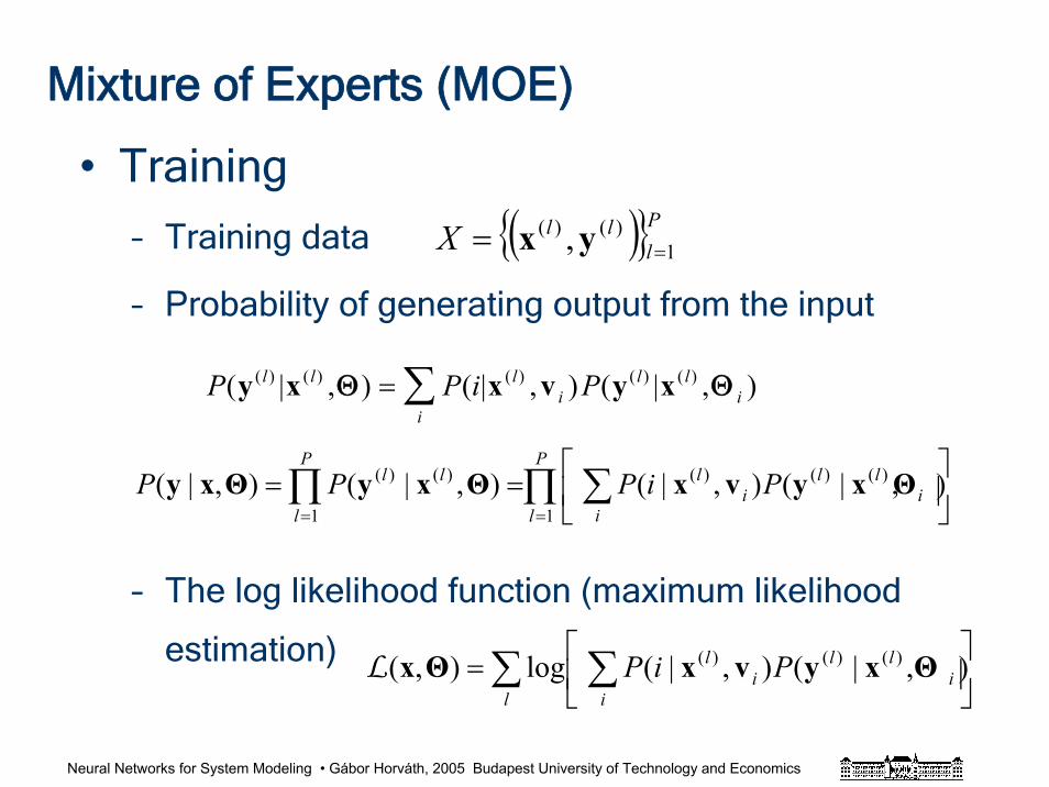
Neural Networks for System Modeling • Gábor Horváth, 2005 Budapest University of Technology and Economics
Mixture of Experts (MOE)
• Training
– Training data
– Probability of generating output from the input
– The log likelihood function (maximum likelihood
estimation)
( ) Pl
llX 1)()( , == yx
P P i Pl l li
l li
i( | , ) ( | , ) ( | , )( ) ( ) ( ) ( ) ( )y x x v y xΘ Θ= ∑
∏ ∑∏==
⎥⎦
⎤⎢⎣
⎡==
P
l ii
lli
lP
l
ll PiPPP1
)()()(
1
)()( ),|(),|(),|(),|( ΘxyvxΘxyΘxy
⎥⎦
⎤⎢⎣
⎡= ∑∑
ii
lli
l
lPiP ),|(),|(log),( )()()( ΘxyvxΘxL
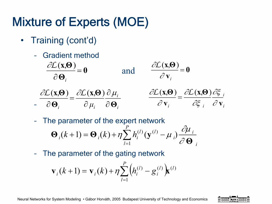
Neural Networks for System Modeling • Gábor Horváth, 2005 Budapest University of Technology and Economics
Mixture of Experts (MOE)
• Training (cont’d)
– Gradient method
–
– The parameter of the expert network
– The parameter of the gating network
and 0vΘx
=i∂
∂ ),(L0
ΘΘx
=∂ i
),(L∂
i
iP
li
lliii hkk
ΘyΘΘ
∂∂μ
μη∑=
−+=+1
)()( )()()1(
( ) )(
1
)()()()1( lP
l
li
liii ghkk xvv ∑
=
−+=+ η
i
i
ii vΘx
vΘx
∂∂ξ
∂ξ∂
∂∂ ),(),( LL
=i
i
ii μ ΘΘx
ΘΘx
∂∂
∂=
∂μ∂∂ ),(),( LL
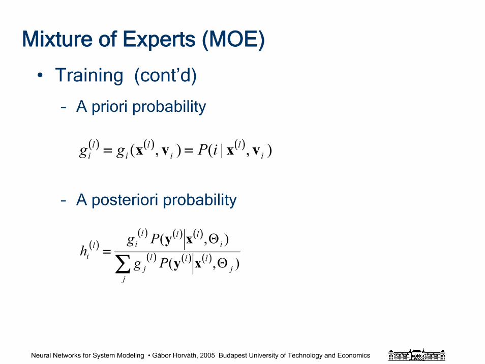
Neural Networks for System Modeling • Gábor Horváth, 2005 Budapest University of Technology and Economics
Mixture of Experts (MOE)
• Training (cont’d)
– A priori probability
– A posteriori probability
( )( ) ( ) ( )
( ) ( ) ( )∑=
jj
lllj
illl
ili Pg
Pgh
),(
),(
Θ
Θ
xy
xy
( ) ( ) ( ) ),|(),( il
il
il
i iPgg vxvx ==
Neural Networks for System Modeling • Gábor Horváth, 2005 Budapest University of Technology and Economics
Mixture of Experts (MOE)
• Training (cont’d)
– EM (Expectation Maximization) algorithm
A general iterative technique for maximum likelihood
estimation
• Introducing hidden variables
• Defining a log-likelihood function
– Two steps:
• Expectation of the hidden variables
• Maximization of the log-likelihood function
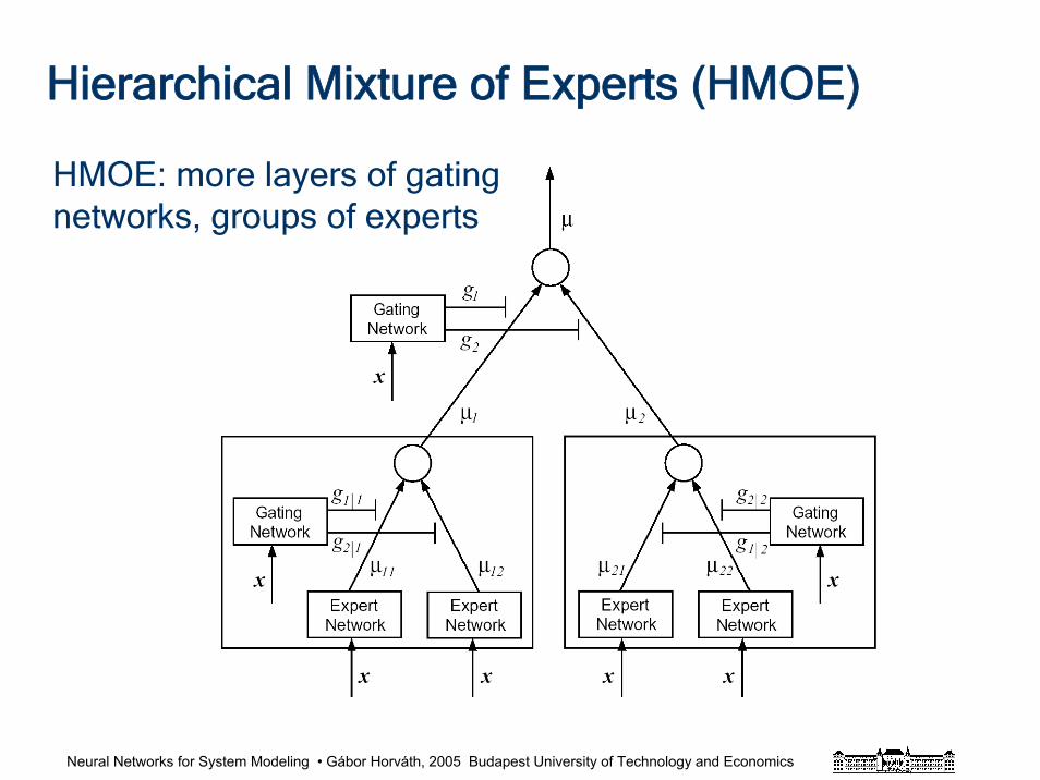
Neural Networks for System Modeling • Gábor Horváth, 2005 Budapest University of Technology and Economics
Hierarchical Mixture of Experts (HMOE)
HMOE: more layers of gating networks, groups of experts
Neural Networks for System Modeling • Gábor Horváth, 2005 Budapest University of Technology and Economics
• MOE construction
• Cross-validation can be used to find the proper
architecture
• CART (Clasification And Regression Tree) for initial
hierarchical MOE (HMOE) architecture and for the initial
expert and gating network parameters
• MOE based on SVMs: different SVMs with different
hyperparameters
Mixture of Experts (MOE)
Neural Networks for System Modeling • Gábor Horváth, 2005 Budapest University of Technology and Economics
References and further readings
Haykin, S.: "Neural Networks. A Comprehensive Foundation" Prentice Hall, N. J.1999. Jordan, M. I., Jacobs, R. A.: “Hierarchical Mixture of Experts and the EM Algorithm”
Neural Computation Vol. 6. pp. 181-214, 1994.Bilmes, J. A. et al “A Gentle Tutorial of the EM Algorithm and its application to Parameter
Estimation for Gaussian Mixture and Hidden Markov Models” 1998.Dempster A.P. et al “Maximum-likelihood from incomplete data via the EM algorithm”,
1977.Moon, T.K.”The Expectation-Maximization Algorithm” IEEE Trans Signal Processing,
1996.

Neural Networks for System Modeling • Gábor Horváth, 2005 Budapest University of Technology and Economics
Application: modelling an industrial plant
(steel converter)
Neural Networks for System Modeling • Gábor Horváth, 2005 Budapest University of Technology and Economics
Overview
• Introduction• Modeling approaches• Building neural models• Data base construction• Model selection• Modular approach• Hybrid approach• Information system• Experiences with the advisory system• Conclusions
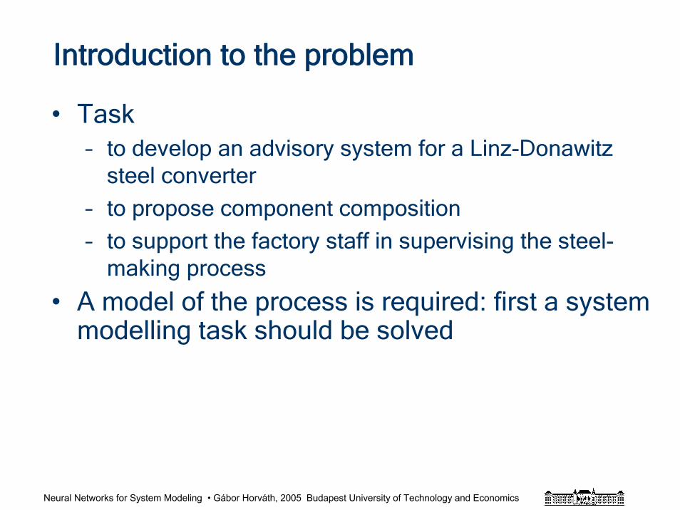
Neural Networks for System Modeling • Gábor Horváth, 2005 Budapest University of Technology and Economics
Introduction to the problem
• Task– to develop an advisory system for a Linz-Donawitz
steel converter
– to propose component composition
– to support the factory staff in supervising the steel-making process
• A model of the process is required: first a system modelling task should be solved

Neural Networks for System Modeling • Gábor Horváth, 2005 Budapest University of Technology and Economics
LD Converter modeling
The Linz-Donawitz
converter in Hungary
(Dunaferr Co.)
Basic Oxigen Steelmaking
(BOS)

Neural Networks for System Modeling • Gábor Horváth, 2005 Budapest University of Technology and Economics
Phases of steelmaking
• 1. Filling of waste iron• 2. Filling of pig iron• 3. Blasting with pure
oxygen• 4. Supplement additives• 5. Sampling for quality
testing• 6. Tapping of steel and
slag
Linz-Donawitz converter

Neural Networks for System Modeling • Gábor Horváth, 2005 Budapest University of Technology and Economics
Phases of steelmaking
• 1. Filling of waste iron• 2. Filling of pig iron• 3. Blasting with pure
oxygen• 4. Supplement additives• 5. Sampling for quality
testing• 6. Tapping of steel and slag
Linz-Donawitz converter
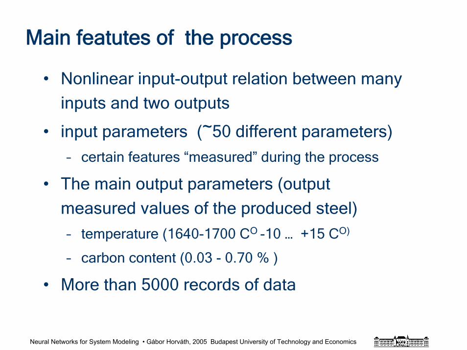
Neural Networks for System Modeling • Gábor Horváth, 2005 Budapest University of Technology and Economics
• Nonlinear input-output relation between many
inputs and two outputs
• input parameters (~50 different parameters)
– certain features “measured” during the process
• The main output parameters (output
measured values of the produced steel)
– temperature (1640-1700 CO -10 … +15 CO)
– carbon content (0.03 - 0.70 % )
• More than 5000 records of data
Main featutes of the process
Neural Networks for System Modeling • Gábor Horváth, 2005 Budapest University of Technology and Economics
• The difficulties of model building
– High complexity nonlinear input-output relationship
– No (or unsatisfactory) physical insight
– Relatively few measurement data
– There are unmeasurable parameters of the process
– Noisy, imprecise, unreliable data
– Classical approach (heat balance, mass balance) gives
no acceptable results
Modeling task
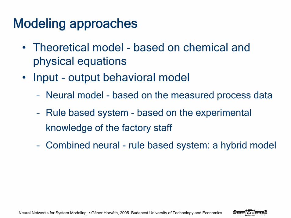
Neural Networks for System Modeling • Gábor Horváth, 2005 Budapest University of Technology and Economics
Modeling approaches
• Theoretical model - based on chemical andphysical equations
• Input - output behavioral model
– Neural model - based on the measured process data
– Rule based system - based on the experimental
knowledge of the factory staff
– Combined neural - rule based system: a hybrid model
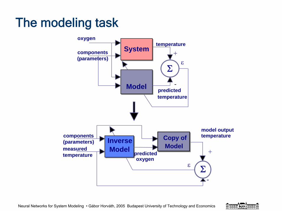
Neural Networks for System Modeling • Gábor Horváth, 2005 Budapest University of Technology and Economics
System
Model
Σε
components(parameters)
temperature
predictedtemperature
+
-
oxygen
measuredtemperature
components(parameters)
Σε
-
+
Copy ofModel
predictedoxygen
InverseModel
model outputtemperature
The modeling task
Neural Networks for System Modeling • Gábor Horváth, 2005 Budapest University of Technology and Economics
Overview
• Introduction• Modeling approaches• Building neural models• Data base construction• Model selection• Modular approach• Hybrid approach• Information system• Experiences with the advisory system• Conclusions
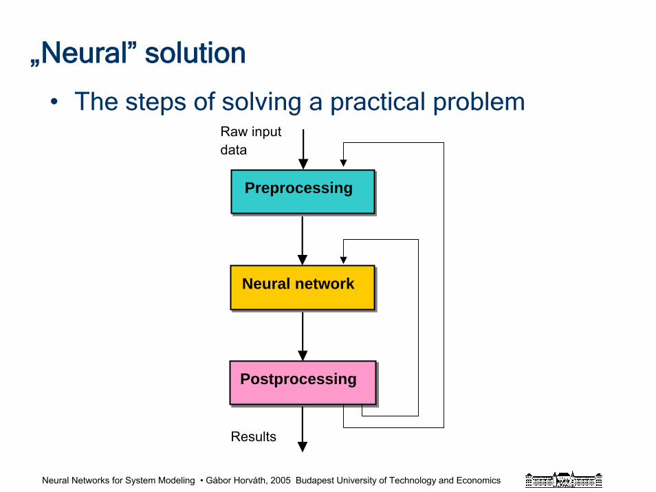
Neural Networks for System Modeling • Gábor Horváth, 2005 Budapest University of Technology and Economics
„Neural” solution
• The steps of solving a practical problem
Preprocessing
Neural network
Postprocessing
Results
Raw input data
Neural Networks for System Modeling • Gábor Horváth, 2005 Budapest University of Technology and Economics
• Creating a reliable database – the problem of noisy data
– the problem of missing data
– the problem of uneven data distribution
• Selecting a proper neural architecture– static network (size of the network)
– dynamic network
• size of the network: nonlinear mapping
• regressor selection + model order selection
• Training and validating the model
Building neural models
Neural Networks for System Modeling • Gábor Horváth, 2005 Budapest University of Technology and Economics
Creating a reliable database
• Input components – measure of importance
• physical insight• sensitivity analysis (importance of the input variables)• mathematical methods: dimension reduction (e.g. PCA)
• Normalization– input normalization– output normalization
• Missing data– artificially generated data
• Noisy data– preprocessing, filtering, – errors-in-variables criterion function, etc.
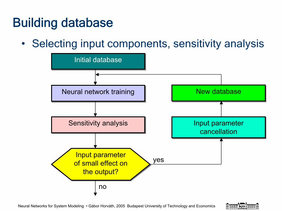
Neural Networks for System Modeling • Gábor Horváth, 2005 Budapest University of Technology and Economics
Building database
• Selecting input components, sensitivity analysis
Initial databaseInitial database
Neural network trainingNeural network training
Sensitivity analysisSensitivity analysis
Input parameter of small effect on
the output?
Input parameter of small effect on
the output?
New databaseNew database
Input parameter cancellation
Input parameter cancellation
no
yes
Neural Networks for System Modeling • Gábor Horváth, 2005 Budapest University of Technology and Economics
Building database
• Dimension reduction: mathematical methods
– PCA
– Non-linear PCA, Kernel PCA
– ICA
• Combined methods
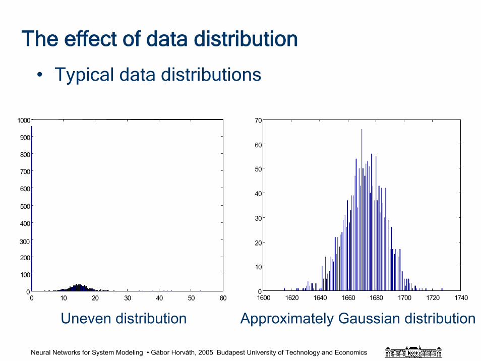
Neural Networks for System Modeling • Gábor Horváth, 2005 Budapest University of Technology and Economics
The effect of data distribution
• Typical data distributions
0 10 20 30 40 50 600
100
200
300
400
500
600
700
800
900
1000
1600 1620 1640 1660 1680 1700 1720 17400
10
20
30
40
50
60
70
Uneven distribution Approximately Gaussian distribution
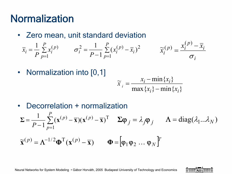
Neural Networks for System Modeling • Gábor Horváth, 2005 Budapest University of Technology and Economics
Normalization
• Zero mean, unit standard deviation
• Normalization into [0,1]
• Decorrelation + normalization
minmaxmin~
ii
iixx
xxx i −−
=
∑==
P
p
pii x
Px
1
)(1∑ −
−=
=
P
pi
pii xx
P 1
2)(2 )(1
1σi
ip
ipi
xxxσ
−=
)()(~
∑=
−−−
=P
p
ppP 1
T)()( ))((1
1 xxxxΣ )...(diag 1 Nλλ=Λ
)(~ )(T2/1)( xxΦx −= − pp Λ
jjj λ ϕϕ =Σ
[ ]TNϕϕϕ K21=Φ
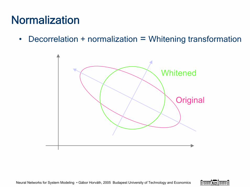
Neural Networks for System Modeling • Gábor Horváth, 2005 Budapest University of Technology and Economics
Normalization
• Decorrelation + normalization = Whitening transformation
Original
Whitened
Neural Networks for System Modeling • Gábor Horváth, 2005 Budapest University of Technology and Economics
Missing or few data
• Filling in the missing values
– based on available information
• Artificially generated data
– using trends
– using correlation
– using realistic transformations
Neural Networks for System Modeling • Gábor Horváth, 2005 Budapest University of Technology and Economics
Overview
• Introduction• Modeling approaches• Building neural models• Data base construction• Model selection• Modular approach• Hybrid approach• Information system• Experiences with the advisory system• Conclusions
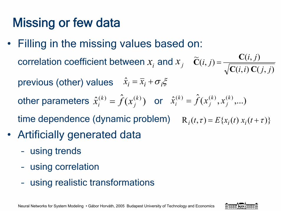
Neural Networks for System Modeling • Gábor Horváth, 2005 Budapest University of Technology and Economics
Missing or few data
• Filling in the missing values based on:
correlation coefficient between and
previous (other) values
other parameters or
time dependence (dynamic problem)
• Artificially generated data
– using trends
– using correlation
– using realistic transformations
),(),(),(),(~
jjiijiji
CCCC =
ξσ iii xx +=ˆ
)(ˆˆ )()( kj
ki xfx =
)()(),(R ττ += txtxEt iii
ix jx
,...),(ˆˆ )()()( kj
kj
ki xxfx =
Neural Networks for System Modeling • Gábor Horváth, 2005 Budapest University of Technology and Economics
Few data
• Artificial data generation
– using realistic transformations
– using sensitivity values: data generation around various
working points (a good example: ALVINN)
(ALVINN = Autonomous Land Vehicle In a Neural Net an onroadneural network navigation solution developed in CMU)
Neural Networks for System Modeling • Gábor Horváth, 2005 Budapest University of Technology and Economics
Noisy data
Inherent noise suppression– classical neural nets have noise suppression property
(inherent regularization)
– Regularization (smoothing regularization)
– averaging (modular approach)
• SVMε-insensitive criterion function
• EIV– input and output noise are taken into consideration
– modified criterion function
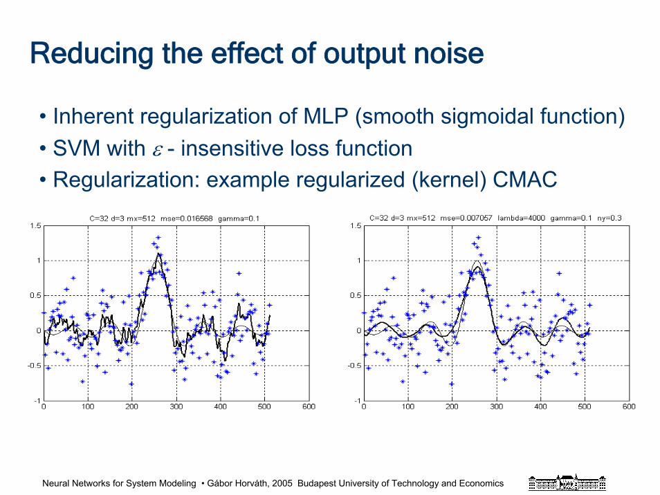
Neural Networks for System Modeling • Gábor Horváth, 2005 Budapest University of Technology and Economics
Reducing the effect of output noise
• Inherent regularization of MLP (smooth sigmoidal function)• SVM with ε - insensitive loss function• Regularization: example regularized (kernel) CMAC
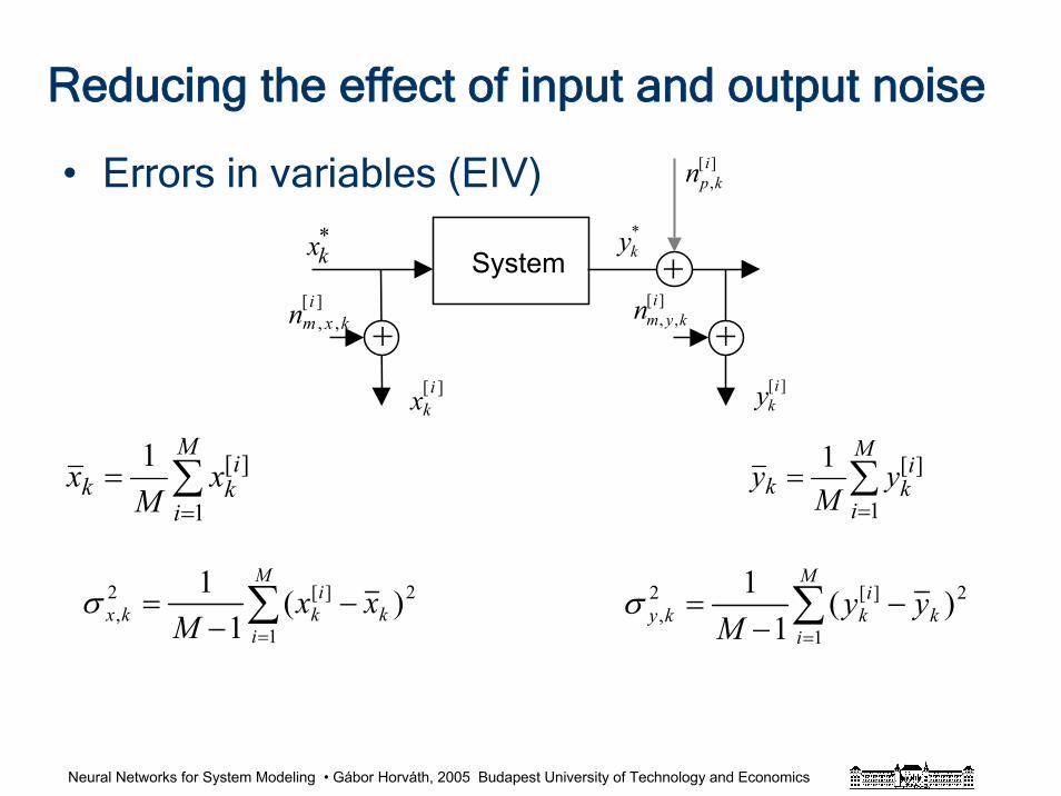
Neural Networks for System Modeling • Gábor Horváth, 2005 Budapest University of Technology and Economics
Reducing the effect of input and output noise
• Errors in variables (EIV)
System][
,,i
kxmn
*kx *
ky
][,
ikpn
][,,
ikymn
][ ikx
][iky
+
+
+
∑=
=M
i
ikk x
Mx
1
][1∑=
=M
i
ikk y
My
1
][1
∑=
−−
=M
ik
ikkx xx
M 1
2][2, )(
11σ ∑
=
−−
=M
ik
ikky yy
M 1
2][2, )(
11σ
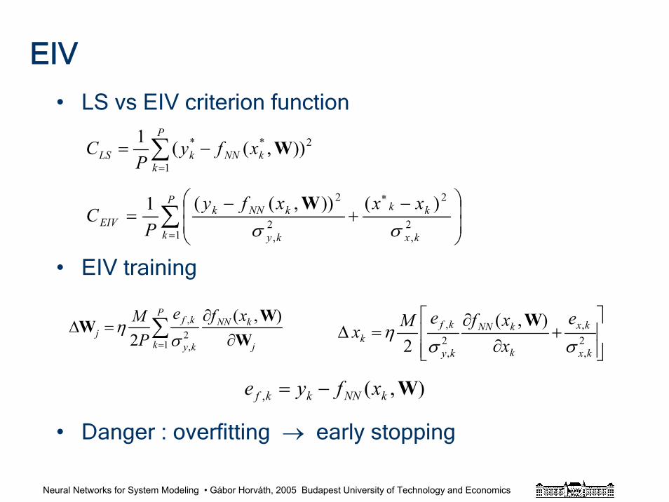
Neural Networks for System Modeling • Gábor Horváth, 2005 Budapest University of Technology and Economics
EIV
• LS vs EIV criterion function
• EIV training
• Danger : overfitting → early stopping
∑= ∂
∂=Δ
P
k j
kNN
ky
kfj
xfeP
M1
2,
, ),(2 W
WW
ση
⎥⎥⎦
⎤
⎢⎢⎣
⎡+
∂∂
=Δ 2,
,2,
, ),(2 kx
kx
k
kNN
ky
kfk
exxfeMx
σση
W
∑=
−=P
kkNNkLS xfy
PC
1
2** )),((1 W
∑=
∗
⎟⎟⎠
⎞⎜⎜⎝
⎛ −+
−=
P
k kx
kk
ky
kNNkEIV
xxxfyP
C1
2,
2
2,
2 )()),((1σσ
W
),(, WkNNkkf xfye −=
Neural Networks for System Modeling • Gábor Horváth, 2005 Budapest University of Technology and Economics
Noisy data
• Output noise is easier to suppress than input noise
• SVM, regularization can reduce the effect of output noise
• EIV (and similar other methods) can take into consideration the input noise
• EIV results in only slightly better approximation
• EIV is rather prone to overfitting (much more free parameters) → early stopping
Neural Networks for System Modeling • Gábor Horváth, 2005 Budapest University of Technology and Economics
Overview
• Introduction• Modeling approaches• Building neural models• Data base construction• Model selection• Modular approach• Hybrid approach• Information system• Experiences with the advisory system• Conclusions
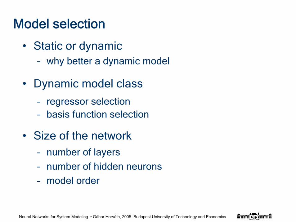
Neural Networks for System Modeling • Gábor Horváth, 2005 Budapest University of Technology and Economics
Model selection
• Static or dynamic– why better a dynamic model
• Dynamic model class
– regressor selection– basis function selection
• Size of the network– number of layers
– number of hidden neurons
– model order
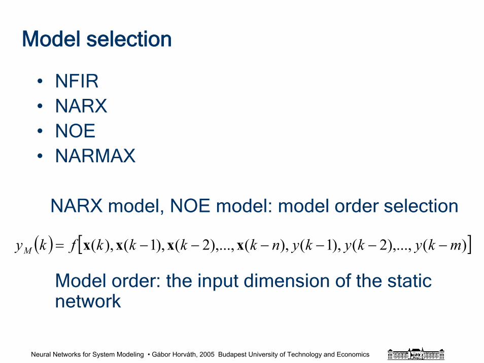
Neural Networks for System Modeling • Gábor Horváth, 2005 Budapest University of Technology and Economics
Model selection
• NFIR• NARX• NOE• NARMAX
NARX model, NOE model: model order selection
Model order: the input dimension of the static network
( ) [ ])(),...,2(),1(),(),...,2(),1(),( mkykykynkkkkfkyM −−−−−−= xxxx
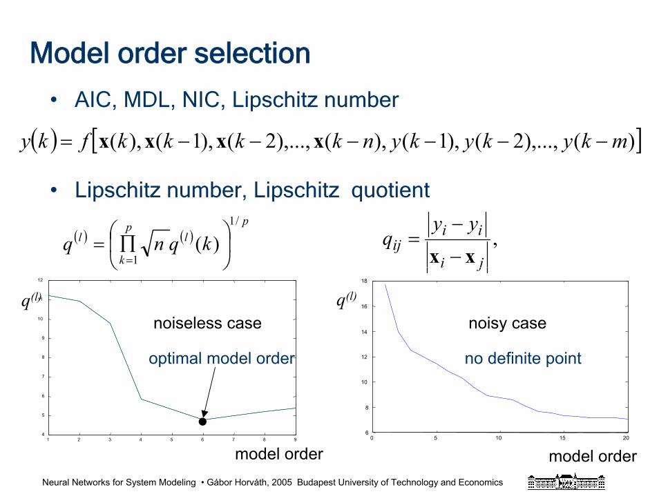
Neural Networks for System Modeling • Gábor Horváth, 2005 Budapest University of Technology and Economics
Model order selection
• AIC, MDL, NIC, Lipschitz number
• Lipschitz number, Lipschitz quotient
( ) [ ])(),...,2(),1(),(),...,2(),1(),( mkykykynkkkkfky −−−−−−= xxxx
( ) ( )p
lp
k
l kqnq/1
1)( ⎟⎠
⎞⎜⎝
⎛ ∏==
,ji
iiij
yyq
xx −
−=
1 2 3 4 5 6 7 8 94
5
6
7
8
9
10
11
12
0 5 10 15 206
8
10
12
14
16
18
q(l) q(l)
model order model order
noiseless case noisy case
•
optimal model order no definite point
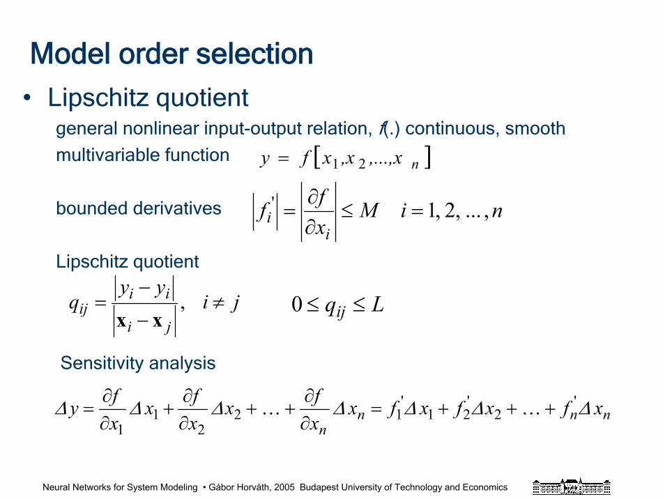
Neural Networks for System Modeling • Gábor Horváth, 2005 Budapest University of Technology and Economics
Model order selection
• Lipschitz quotientgeneral nonlinear input-output relation, f(.) continuous, smooth
multivariable function
bounded derivatives
Lipschitz quotient
Sensitivity analysis
[ ]n,...,x,xxfy 21=
niMxffi
i ,...,2,1' =≤∂∂
=
jiyy
qji
iiij ≠
−
−= ,
xxLqij ≤≤0
nnnn
xfxfxfxxfx
xfx
xfy ΔΔΔΔΔΔΔ '
2'
21'
122
11
+++=∂∂
++∂∂
+∂∂
= KK
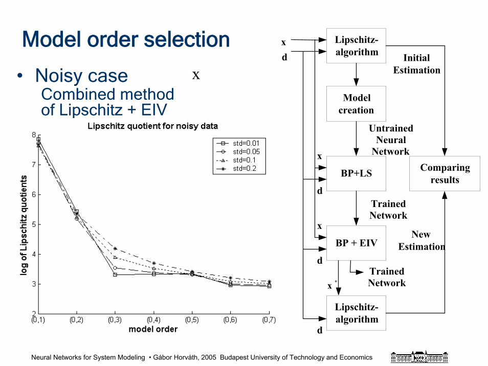
Neural Networks for System Modeling • Gábor Horváth, 2005 Budapest University of Technology and Economics
Model order selection
• Noisy caseCombined method of Lipschitz + EIV
Lipschitz-algorithm
Modelcreation
BP + EIV
BP+LS
Lipschitz-algorithm
Comparingresults
InitialEstimation
xd
x
x
d
d
dTrainedNetwork
*x
NewEstimation
UntrainedNeural
Network
TrainedNetwork
x
Neural Networks for System Modeling • Gábor Horváth, 2005 Budapest University of Technology and Economics
Correlation based model order selection
• Model order 2...4 because of prcatical problems
• Too many input components
• (2...4) * (number of input components + outputs)
• Too large network
• Too few training data
• The problem of missing data
• Network size: cross-validation
Neural Networks for System Modeling • Gábor Horváth, 2005 Budapest University of Technology and Economics
References and further readingsBerényi, P.,, Horváth, G., Pataki, B., Strausz, Gy. : "Hybrid-Neural Modeling of a Complex Industrial
Process" Proc. of the IEEE Instrumentation and Measurement Technology Conference, IMTC'2001. Budapest, May 21-23. Vol. III. pp. 1424-1429.
Horváth, G., Pataki, B. Strausz, T.: "Neural Modeling of a Linz-Donawitz Steel Converter: Difficulties and Solutions" Proc. of the EUFIT'98, 6th European Congress on Intelligent Techniques and Soft Computing. Aachen, Germany. 1998. Sept. pp.1516-1521
Horváth, G. Pataki, B. Strausz, Gy.: "Black box modeling of a complex industrial process", Proc. Of the 1999 IEEE Conference and Workshop on Engineering of Computer Based Systems, Nashville, TN, USA. 1999. pp. 60-66
Pataki, B., Horváth, G., Strausz, Gy., Talata, Zs. "Inverse Neural Modeling of a Linz-Donawitz SteelConverter" e & i Elektrotechnik und Informationstechnik, Vol. 117. No. 1. 2000. pp.
Strausz, Gy., G. Horváth, B. Pataki : "Experiences from the results of neural modelling of an industrialprocess" Proc. of Engineering Application of Neural Networks, EANN'98, Gibraltar 1988. pp. 213-220
Akaike, H. “A New Look at the Statistical Model Identification”, IEEE Transaction on Aut. Control Vol. AC-19, No.6., 1974, pp.716-723
Rissanen, J. “Estimation of Structure by Minimum Description Length”, Circuits, Systems and Signal Processing, special issue on Rational Approximations, Vol. 1, No. 3-4, 1982, pp. 395-406.
Akaike, H. “Statistical Predictor Identification”, Ann. Istitute of Statistical Mathematics, Vol. 22., 1970, pp. 203-217.
He, X. and Asada, H.“A New Method for Identifying Orders of Input-output Models for Nonlinear Dynamic Systems” Proceedings of the American Control Conference, San Francisco, California, June 1993, pp. 2520-2523.
Neural Networks for System Modeling • Gábor Horváth, 2005 Budapest University of Technology and Economics
Overview
• Introduction• Modeling approaches• Building neural models• Data base construction• Model selection• Modular approach• Hybrid approach• Information system• Experiences with the advisory system• Conclusions
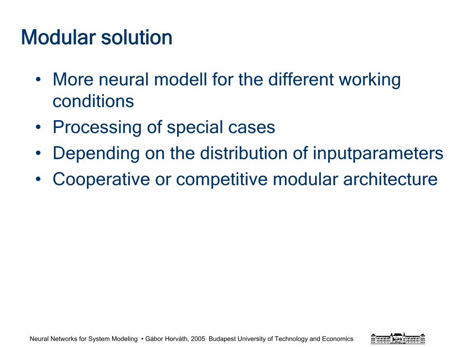
Neural Networks for System Modeling • Gábor Horváth, 2005 Budapest University of Technology and Economics
Modular solution
• More neural modell for the different working conditions
• Processing of special cases
• Depending on the distribution of inputparameters
• Cooperative or competitive modular architecture
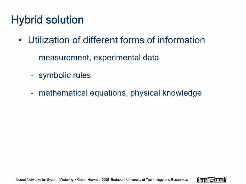
Neural Networks for System Modeling • Gábor Horváth, 2005 Budapest University of Technology and Economics
Hybrid solution
• Utilization of different forms of information
– measurement, experimental data
– symbolic rules
– mathematical equations, physical knowledge
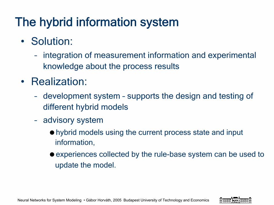
Neural Networks for System Modeling • Gábor Horváth, 2005 Budapest University of Technology and Economics
• Solution: – integration of measurement information and experimental
knowledge about the process results
• Realization:– development system – supports the design and testing of
different hybrid models
– advisory system
hybrid models using the current process state and input information,
experiences collected by the rule-base system can be used to
update the model.
The hybrid information system
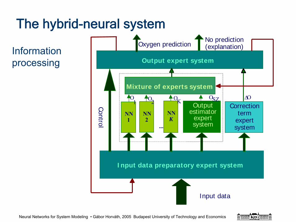
Neural Networks for System Modeling • Gábor Horváth, 2005 Budapest University of Technology and Economics
NNK
O1 O2
OKOSZ ΔO
NN2
NN1
...
Correction term
expert system
Output estimator
expert system
Input data preparatory expert system
Output expert system
Mixture of experts system
Input dataControl
Oxygen predictionNo prediction (explanation)
The hybrid-neural system
Information processing
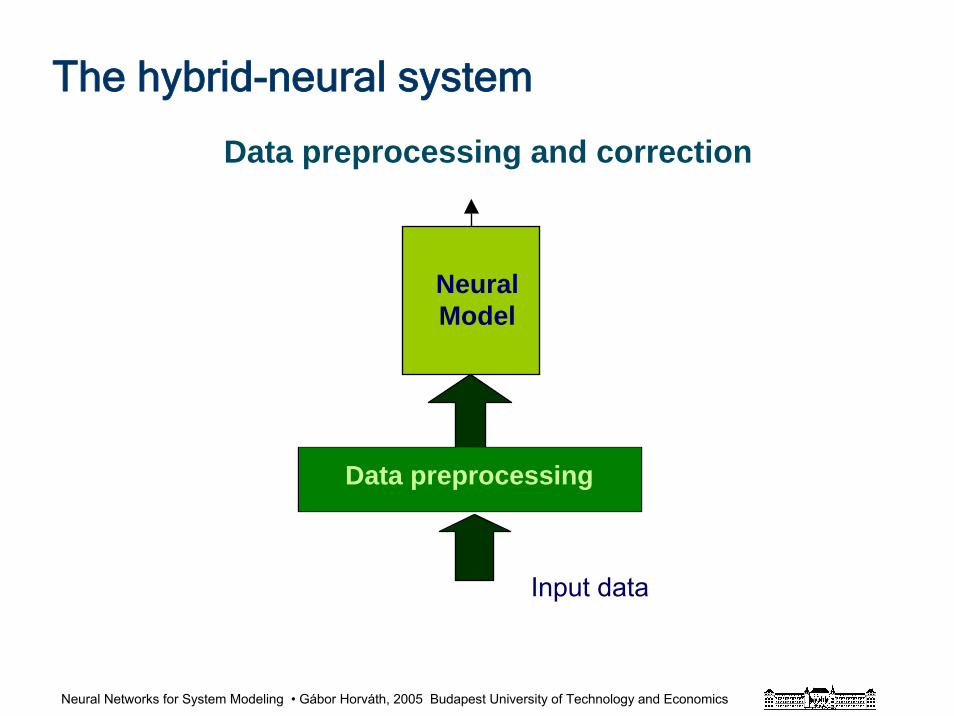
Neural Networks for System Modeling • Gábor Horváth, 2005 Budapest University of Technology and Economics
Neural Model
Data preprocessing
Input data
Data preprocessing and correction
The hybrid-neural system
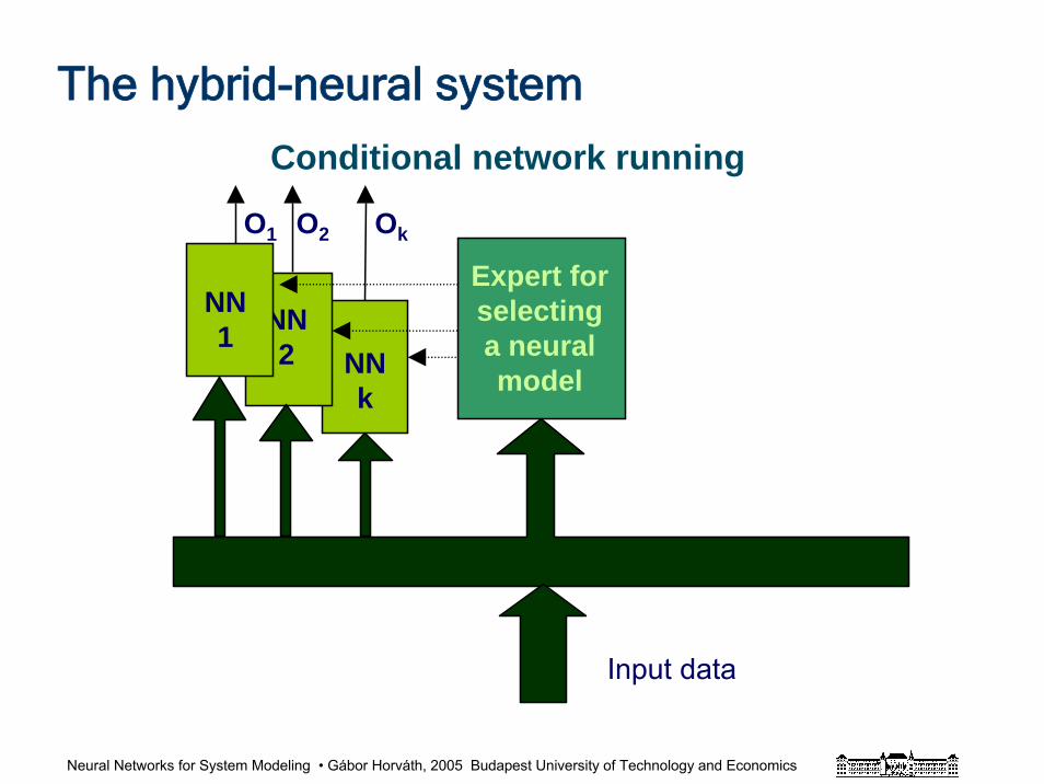
Neural Networks for System Modeling • Gábor Horváth, 2005 Budapest University of Technology and Economics
Expert for selecting a neural model
NN 2
NN 1
NN k
Input data
OkO2O1
Conditional network running
The hybrid-neural system
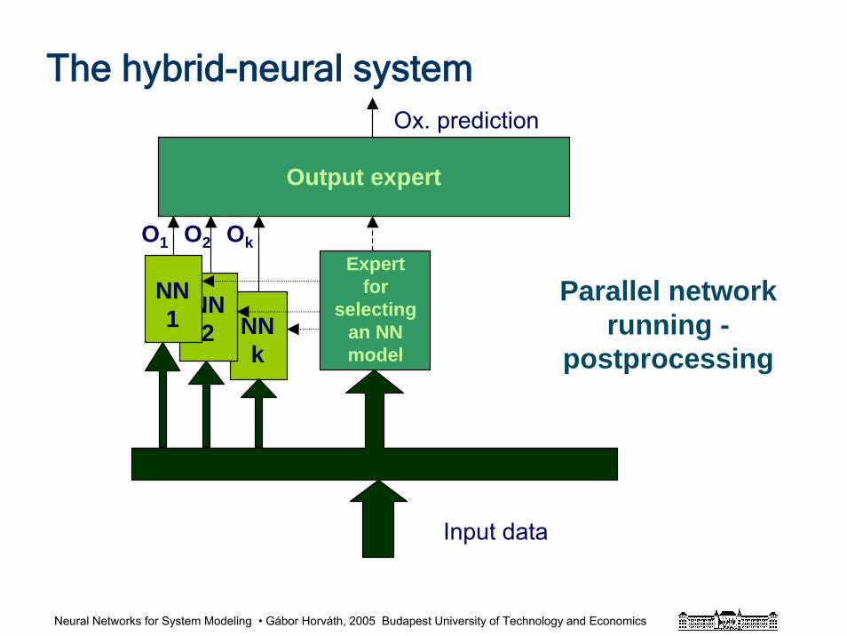
Neural Networks for System Modeling • Gábor Horváth, 2005 Budapest University of Technology and Economics
NN k
NN 2
Expertfor
selecting an NN model
Output expert
Input data
NN 1
Ox. prediction
O1 O2 Ok
Parallel network running -
postprocessing
The hybrid-neural system
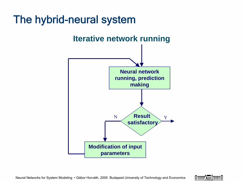
Neural Networks for System Modeling • Gábor Horváth, 2005 Budapest University of Technology and Economics
Result satisfactory
N Y
Neural network running, prediction
making
Modification of input parameters
Iterative network running
The hybrid-neural system
Neural Networks for System Modeling • Gábor Horváth, 2005 Budapest University of Technology and Economics
Validation
• Model selection– iterative process
– utilization of domain knowledge
• Cross validation– fresh data
– on-site testing
Neural Networks for System Modeling • Gábor Horváth, 2005 Budapest University of Technology and Economics
• The hit rate is increased by + 10%
• Most of the special cases can be handled
• Further rules for handling special cases should be obtained
• The accuracy of measured data should be increased
Experiences
Neural Networks for System Modeling • Gábor Horváth, 2005 Budapest University of Technology and Economics
• For complex industrial problems all available information have to be used
• Thinking about NNs as universal modeling devices alone
• Physical insight is important
• The importance of preprocessing and post-processing
• Modular approach: – decomposition of the problem
– cooperation and competition
– “experts” using different paradigms
• The hybrid approach to the problem provided better results
Conclusions
Neural Networks for System Modeling • Gábor Horváth, 2005 Budapest University of Technology and Economics
Summary
• Main questions
• Open questions
• Final conclusions
Neural Networks for System Modeling • Gábor Horváth, 2005 Budapest University of Technology and Economics
Main questions
• Neural modeling: black-box or not?
• When to apply neural approach?
• How to use neural networks?
• The role of prior knowledge
• How to use prior knowledge?
• How to validate the results?
Neural Networks for System Modeling • Gábor Horváth, 2005 Budapest University of Technology and Economics
Open (partly open) questions
• Model class selection
• Model order selection
• Validation, generalization capability
• Sample size, training set, test set, validation set
• Missing data, noisy data, few data
• Data consistency
Neural Networks for System Modeling • Gábor Horváth, 2005 Budapest University of Technology and Economics
Final coclusions• Neural networks are especially important and proper architectures
for (nonlinear) system modelling• General solutions: NN and fuzzy-neural systems are universal
modeling devices (universal approximators)• The importance of the theoretical results, theoretical background• The difficulty of the application of theoretical results in practice• The role of data base• The importance of prior information, physical insight• The importance of preprocessing and post-processing • Modular approach:
– decomposition of the problem– cooperation and competition– “experts” using different paradigms
• Hybrid solutions: combination of rule based, fuzzy, neural,mathematical
Neural Networks for System Modeling • Gábor Horváth, 2005 Budapest University of Technology and Economics
References and further readingsParag H. Batavia, Dean A. Pomerleau, Charles E. Thorpe.: „Applying Advanced Learning Algorithms to
ALVINN”, Technical Report, CMU-RI-TR-96-31 Robotics Institute Carnegie Mellon University Pittsburgh, Pennsylvania 15213-3890
Berényi, P.,, Horváth, G., Pataki, B., Strausz, Gy. : "Hybrid-Neural Modeling of a Complex Industrial Process" Proc. of the IEEE Instrumentation and Measurement Technology Conference, IMTC'2001. Budapest, May 21-23. Vol. III. pp. 1424-1429.
Berényi P., Valyon J., Horváth, G. : "Neural Modeling of an Industrial Process with Noisy Data" IEA/AIE-2001, The Fourteenth International Conference on Industrial & Engineering Applications of Artificial Intelligence & Expert Systems, June 4-7, 2001, Budapest in Lecture Notes in Computer Sciences, 2001, Springer, pp. 269-280.
Bishop, C, M.: “Neural Networks for Pattern Recognition” Clanderon Press, Oxford, 1995.
Horváth, G., Pataki, B. Strausz, T.: "Neural Modeling of a Linz-Donawitz Steel Converter: Difficulties and Solutions" Proc. of the EUFIT'98, 6th European Congress on Intelligent Techniques and Soft Computing. Aachen, Germany. 1998. Sept. pp.1516-1521
Horváth, G. Pataki, B. Strausz, Gy.: "Black box modeling of a complex industrial process", Proc. Of the 1999 IEEE Conference and Workshop on Engineering of Computer Based Systems, Nashville, TN, USA. 1999. pp. 60-66
Pataki, B., Horváth, G., Strausz, Gy., Talata, Zs. "Inverse Neural Modeling of a Linz-Donawitz SteelConverter" e & i Elektrotechnik und Informationstechnik, Vol. 117. No. 1. 2000. pp.
Neural Networks for System Modeling • Gábor Horváth, 2005 Budapest University of Technology and Economics
References and further readingsStrausz, Gy., G. Horváth, B. Pataki : "Experiences from the results of neural modelling of an
industrial process" Proc. of Engineering Application of Neural Networks, EANN'98, Gibraltar 1988. pp. 213-220
Strausz, Gy., G. Horváth, B. Pataki : "Effects of database characteristics on the neural modelingof an industrial process" Proc. of the International ICSC/IFAC Symposium on Neural Computation / NC’98, Sept. 1998, Vienna pp. 834-840.
Bishop, C, M.: “Neural Networks for Pattern Recognition” Clanderon Press, Oxford, 1995.
Horváth, G (ed.),” Neural Networks and Their Applications”, Publishing house of the Budapest University of Technology and Economics, Budapest, 1998. (in Hungarian)
Jang, J. -S. R., Sun, C. -T. and Mizutani: E. „Neuro-Fuzzy and Soft Computing. A Computational Approach to Learning and Machine Intelligence”, Prentice Hall, 1997.
Jang, J. -S. R: „ANFIS: Adaptive-Network-Based Fuzzy Inference System” IEEE Trans. on Sysytem Man, and Cybernetics. Vol. 23. No.3. pp. 665-685, 1993.
Nguyen, D. and Widrow, B. (1989). "The Truck Backer-Upper: An Example of Self-Learning in Neural Networks," in Proceedings of the International Joint Conference on Neural Networks(Washington, DC 1989), vol. II, 357-362.
Rumelhart, D. E., Hinton, G. E., and Williams, R. J. (1986b). "Learning Internal Representations by Error Propagation," in Parallel Distributed Processing: Explorations in the Microstructure of Cognition, vol. I, D. E. Rumelhart, J. L. McClelland, and the PDP Research Group. MIT Press, Cambridge (1986).