Neural Networks - cs.cmu.edubhiksha/courses/mlsp.fall2017/lectures/lec... · Neural Network 18797/11755 15. ... •A multi-layer perceptron is a universal function approximator

Neural Networks

Class 22: MLSP, Fall 2017

Instructor: Bhiksha Raj

IMPORTANT ADMINSTRIVIA

• Final week. Project presentations on 7th

• Abstracts for projects (half page – one page) due on 6th

• Posters due by 6th if you want us to print them

– Poster details will be sent out shortly

18797/11755 2

Neural Networks are taking over!

• Neural networks have become one of the major thrust areas recently in various pattern recognition, prediction, and analysis problems

• In many problems they have established the state of the art

– Often exceeding previous benchmarks by large margins

18797/11755 3

Recent success with neural networks

• Some recent successes with neural networks– A bit of hyperbole, but still..

18797/11755 4


• Some recent successes with neural networks

18797/11755 5


• Some recent successes with neural networks

18797/11755 6


• Some recent successes with neural networks18797/11755 7


• Captions generated entirely by a neural network 18797/11755 8

Successes with neural networks

• And a variety of other problems:

– Image recognition

– Signal enhancement

– Even predicting stock markets!

18797/11755 9

So what are neural networks??

• What are these boxes?

N.NetVoice signal Transcription N.NetImage Text caption

N.NetGameState Next move

18797/11755 10

So what are neural networks??

• It began with this..

• Humans are very good at the tasks we just saw

• Can we model the human brain/ human intelligence?

– An old question – dating back to Plato and Aristotle.. 18797/11755 11

Observation: The Brain

• Mid 1800s: The brain is a mass of interconnected neurons

18797/11755 12

Brain: Interconnected Neurons

• Many neurons connect in to each neuron

• Each neuron connects out to many neurons

18797/11755 13

The brain is a connectionist machine

• The human brain is a connectionist machine

– Bain, A. (1873). Mind and body. The theories of their relation. London: Henry King.

– Ferrier, D. (1876). The Functions of the Brain. London: Smith, Elder and Co

• Neurons connect to other neurons. The processing/capacity of the brain is a function of these connections

• Connectionist machines emulate this structure

18797/11755 14

Connectionist Machines

• Neural networks are connectionist machines– As opposed to Von Neumann Machines

• The machine has many processing units– The program is the connections between these units

• Connections may also define memory

PROCESSOR

PROGRAM

DATA

MemoryProcessingunit

Von Neumann Machine

NETWORK

Neural Network

18797/11755 15

Modelling the brain

• What are the units?

• A neuron:

• Signals come in through the dendrites into the Soma

• A signal goes out via the axon to other neurons

– Only one axon per neuron

• Factoid that may only interest me: Neurons do not undergo cell division

Dendrites

Soma

Axon

18797/11755 16

McCullough and Pitts

• The Doctor and the Hobo..

– Warren McCulloch: Neurophysician

– Walter Pitts: Homeless wannabe logician who arrived at his door

18797/11755 17

The McCulloch and Pitts model

• A mathematical model of a neuron

– McCulloch, W.S. & Pitts, W.H. (1943). A Logical Calculus of the Ideas Immanent in Nervous Activity, Bulletin of Mathematical Biophysics, 5:115-137, 1943

– Threshold Logic

• Note: McCullough and Pitts original model was actually slightly different – this model is actually due to Rosenblatt

A single neuron

18

The solution to everything

• Frank Rosenblatt

– Psychologist, Logician

– Inventor of the solution to everything, aka the Perceptron (1958)

• A mathematical model of the neuron that could solve everything!!! 19

Simplified mathematical model

• Number of inputs combine linearly

– Threshold logic: Fire if combined input exceeds

threshold

𝑌 = ൞1 𝑖𝑓

𝑖

𝑤𝑖𝑥𝑖 + 𝑏 > 0

0 𝑒𝑙𝑠𝑒18797/11755 20

Simplified mathematical model

• A mathematical model

– Originally assumed could represent any Boolean circuit

– Rosenblatt, 1958 : “the embryo of an electronic computer

that [the Navy] expects will be able to walk, talk, see,

write, reproduce itself and be conscious of its existence”

18797/11755 21

Perceptron

• Boolean Gates

• But…

X

Y

1

1

2

X

Y

1

1

1

0X-1

X ∧ Y

X ∨ Y

ഥX

18797/11755 22

Perceptron

X

Y

?

?

? X⨁Y

No solution for XOR!Not universal!

• Minsky and Papert, 1968

18797/11755 23

A single neuron is not enough

• Individual elements are weak computational elements– Marvin Minsky and Seymour Papert, 1969, Perceptrons:

An Introduction to Computational Geometry

• Networked elements are required

18797/11755 24

Multi-layer Perceptron!

• XOR

– The first layer is a “hidden” layer

25

1

1

1

-1

1

-1

X

Y

1

X⨁Y

-1

2

X ∨ Y

ഥX ∨ ഥY

Hidden Layer

18797/11755

Multi-Layer Perceptron

• Even more complex Boolean functions can be composed using layered networks of perceptrons

– Two hidden layers in above model

– In fact can build any Boolean function over any number of inputs26

( 𝐴& ത𝑋&𝑍 | 𝐴& ത𝑌 )&( 𝑋 & 𝑌 | 𝑋&𝑍 )

12 1 1 12 1 1

X Y Z A

10 11

12

11 1-111 -1

1 1

1 -1 1 1

11

18797/11755

Multi-layer perceptrons are universal Boolean functions

• A multi-layer perceptron is a universal Boolean function

• In fact, an MLP with only one hidden layer is a universal Boolean function!

18797/11755 27

Neural Networks: Multi-layer Perceptrons

• In reality the input to these systems is not Boolean

• Inputs are continuous valued– Signals may be continuous valued

– Image features are continuous valued

– Pixels are multi-valued (e.g. 0-255)


29

MLP on continuous inputs

• The inputs are continuous valued

– Threshold logic: Fire if combined input exceeds

threshold

𝑌 = ൞1 𝑖𝑓

𝑖

𝑤𝑖𝑥𝑖 + 𝑏 > 0

0 𝑒𝑙𝑠𝑒18797/11755 30

A Perceptron on Reals

• A perceptron operates on real-valued vectors– This is just a linear classifier

31

x1

x2

w1,w2

𝑦 = ൞1 𝑖𝑓

𝑖

𝑤𝑖x𝑖 ≥ 𝑇

0 𝑒𝑙𝑠𝑒

x1

x2

18797/11755

Booleans over the reals

• The network must fire if the input is in the coloured area

32

x1

x2Can now be composed into“networks” to compute arbitraryclassification “boundaries”

18797/11755



33

x1

x2

x1x2

18797/11755



34

x1

x2

x1x2

18797/11755



35

x1

x2

x1x2

18797/11755



36

x1

x2

x1x2

18797/11755



37

x1

x2

x1x2

18797/11755



38

x1

x2

x1

x2

AND

5

44

4

4

4

3

3

3

33 x1x2

𝑖=1

𝑁

y𝑖 ≥ 𝑁?

y1 y5y2 y3 y4

18797/11755


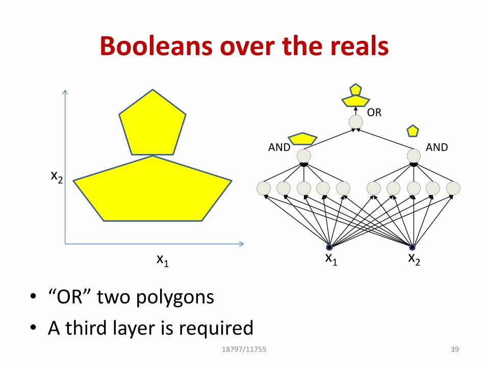
• “OR” two polygons

• A third layer is required39

x2

AND AND

OR

x1 x1 x2

18797/11755

How Complex Can it Get

• An arbitrarily complex decision boundary

• Basically any Boolean function over the basic linear boundaries

4018797/11755

Story so far..

• Multi-layer perceptrons are Boolean networks

– They represent Boolean functions over linear boundaries

– They can approximate any boundary

• Using a sufficiently large number of linear units

4518797/11755

MLP as a continuous-valued regression

• MLPs can actually compose arbitrary functions to arbitrary precision

– Not just classification/Boolean functions

• 1D example

– Left: A net with a pair of units can create a pulse of any width at any location

– Right: A network of N such pairs approximates the function with N scaled pulses52

x

1T1

T2

1

T1

T2

1

-1T1 T2 x

f(x)x

+× ℎ1× ℎ2

× ℎ𝑛

ℎ1

ℎ2

ℎ𝑛

+

MLP as a continuous-valued regression

• MLPs can actually compose arbitrary functions– Even with only one layer

– To arbitrary precision

– The MLP is a universal approximator!

53

× ℎ1

× ℎ2

× ℎ𝑛

ℎ1ℎ2

ℎ𝑛

18797/11755

Multi-layer perceptrons are universal function approximators

• A multi-layer perceptron is a universal function approximator

– Hornik, Stinchcombe and White 1989, several others

N.NetX, Y Z, Colour

18797/11755 54

What’s inside these boxes?

• Each of these tasks is performed by a net like this one– Functions that take the given input and produce the

required output



18797/11755 55

Story so far

• MLPs are Boolean machines

– They represent arbitrary Boolean functions over arbitrary linear boundaries

– MLPs perform classification

• MLPs can compute arbitrary real-valued functions of arbitrary real-valued inputs

– To arbitrary precision

– They are universal approximators

5618797/11755

• Building a network for a task

18797/11755 57

These tasks are functions

• Each of these boxes is actually a function

– E.g f: Image Caption



18797/11755 58

These tasks are functions

Voice signal Transcription Image Text caption

GameState Next move

• Each box is actually a function

– E.g f: Image Caption

– It can be approximated by a neural network59

The network as a function

• Inputs are numeric vectors

– Numeric representation of input, e.g. audio, image, game state, etc.

• Outputs are numeric scalars or vectors

– Numeric “encoding” of output from which actual output can be derived

– E.g. a score, which can be compared to a threshold to decide if the input is a face or not

– Output may be multi-dimensional, if task requires it

Input Output

18797/11755 60

The network is a function

• Given an input, it computes the function layer wise to predict an output

18797/11755 61

A note on activations

• Previous explanations assumed network units used a threshold function for “activation”

• In reality, we use a number of other differentiable functions

– Mostly, but not always, “squashing” functions 62

x1

x2

x3

xN

sigmoid tanh

The entire network

• Inputs (D-dimensional): 𝑋1, … , 𝑋𝐷

• Weights from ith node in lth layer to jth node in l+1th layer: 𝑊𝑖,𝑗𝑙

• Complete set of weights

{𝑊𝑖,𝑗𝑙 ; 𝑙 = 0. . 𝐿, 𝑖 = 1…𝑁𝑙 , 𝑗 = 1…𝑁𝑙+1}

• Outputs (M-dimensional): 𝑂1, … , 𝑂𝑀18797/11755 63

Making a prediction (Aka forward pass)

⋮ ⋮ ⋮⋮𝑋Illustration with a

network withN-1 hidden layers ⋮⋮⋮ 𝑓𝑁

𝑂⋯

18797/11755 64

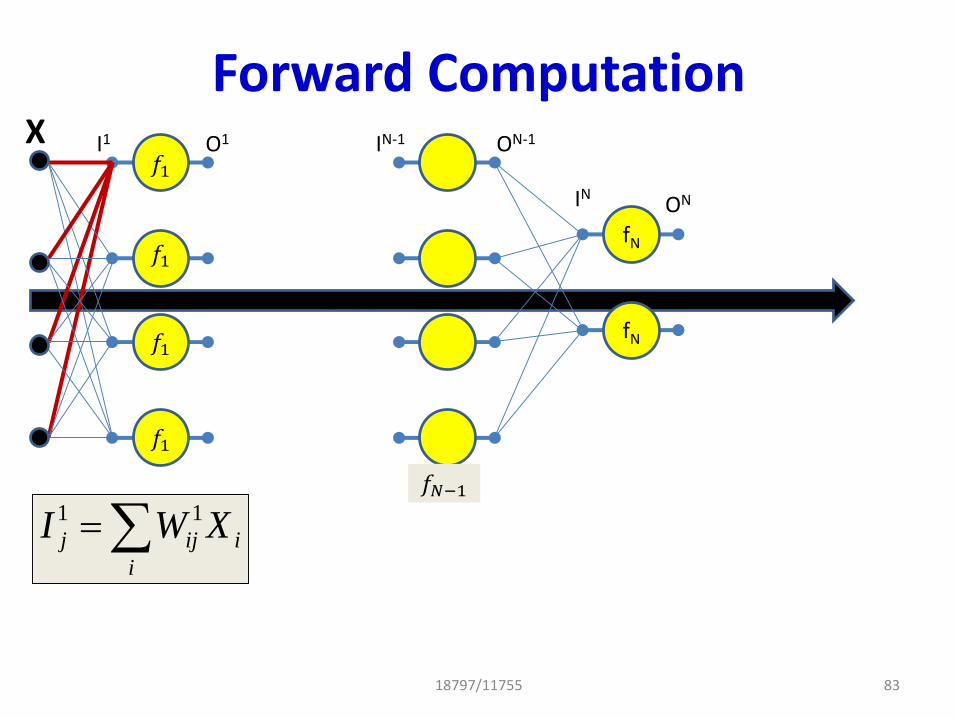
Forward Computation

i

i

ijj XWI 11

fN

fN

⋯

𝑓1

𝑓𝑁−1

ONIN

ON-1IN-1O1I1X

𝑓1

𝑓1

𝑓1

For the jth neuron of the 1st hidden layer:Input to the activation functions in the first layer

18797/11755 65

Forward Computation

i

i

ijj XWI 11

fN

fN

⋯

𝑓1

𝑓𝑁−1

ONIN

ON-1IN-1O1I1X

𝑓1

𝑓1

𝑓1

For the jth neuron of the 1st hidden layer:Input to the activation functions in the first layer

)( 1

1

1

jj IfO Output of the jth neuron of the 1st hidden layer:18797/11755 66

Forward Computation

1 k

i

i

k

ij

k

j OWI

fN

fN

⋯

𝑓𝑘 𝑓𝑁−1

ONIN

ON-1IN-1OkIkOk-1Ik-1

⋯

For the jth neuron of the kth hidden layer:Input to the activation functions in the kth layer

18797/11755 67

Forward Computation

1 k

i

i

k

ij

k

j OWI )( k

jk

k

j IfO

fN

fN

⋯


ONIN


⋯

Output of the jth neuron of the kth hidden layer:

For the jth neuron of the kth hidden layer:Input to the activation functions in the kth layer

18797/11755 68

Forward Computation

i

i

ijj XWI 11

1 k

i

i

k

ij

k

j OWI

)( k

jk

k

j IfO

fN

fN

⋯


ONIN


⋯

ITERATE FOR k = 1:N

for j = 1:layer-width

Output ON is the output of the network18797/11755 69

The problem of training the network

• The network must be composed correctly to produce the desired outputs

• This is the problem of “training” the network

18797/11755 70

The Problem of Training a Network

• A neural network is effectively just a function– What makes it an NNet is the structure of the function

• Takes an input– Generally multi-dimensional

• Produces an output– May be uni- or multi-dimensional

• Challenge: How to make it produce the desired output for any given input

f(x)X Y = f(X) X Y = f(X)

18797/11755 71

Building by design

• Solution 1: Just hand design it– What will the network for the above function be?

• We can hand draw this one..

X1X2

Y

X1

X2

18797/11755 72

• Most functions are too complex to hand-design– Particularly in high-dimensional spaces

• Instead, we will try to learn it from “training” examples– Input-output pairs

– In reality the training data will not be even remotely as dense as shown in the figure

• It will be several orders of magnitude sparser

Training from examples

73

General approach to training

• Define an error between the actual network output for any parameter value and the desired output

– Error can be defined in a number of ways

• Many “Divergence” functions have been defined

– Typically defined as the sum of the error over individual training instances

Blue lines: error whenfunction is below desiredoutput

Black lines: error whenfunction is above desiredoutput

18797/11755 74

Recall: A note on activations

• Composing/learning networks using threshold “activations” is a combinatorial problem

– Exponentially hard to find the right solution

• The smoother differentiable activation functions enable learning through optimization 75

x1

x2

x3

xN

sigmoid tanh

Minimizing Error

• Problem: Find the parameters at which this function achieves a minimum

– Subject to any constraints we may pose

– Typically, this cannot be found using a closed-form formula

ERR

OR

18797/11755 76

The Approach of Gradient Descent

• Iterative solution:

– Start at some point

– Find direction in which to shift this point to decrease error• This can be found from the “slope” of the function

– A positive slope moving left decreases error

– A negative slope moving right decreases error

– Shift point in this direction• The size of the shift depends on the slope18797/11755 77


• Multi-dimensional function:

– “Slope” replaced by vector “gradient”

• From current point shift in direction opposite to gradient

– Size of shift depends on magnitude of gradient

y

yxfx

yxf

f),(

),(

18797/11755 78


• The gradient descent algorithm𝑊 ← 𝑊 − 𝜂𝛻𝑊𝐸 𝑋;𝑊

Until error E(X;W) converges

𝜂 is the “step size”

Steps are smaller when the “slope”is smaller, because the optimum value is generally at a location of near-zero slope

18797/11755 79


• The gradient descent algorithm𝑊 ← 𝑊 − 𝜂𝛻𝑊𝐸 𝑋;𝑊

Until error E(X;W) converges

𝜂 is the “step size”

Steps are smaller when the “slope”is smaller, because the optimum value is generally at a location of near-zero slope

Needs computation of gradient oferror w.r.t. network parameters

18797/11755 80

Gradients: Algebraic Formulation

• The network is a nested function𝑜 = 𝑓𝑁(𝑊𝑁𝑓𝑁−1 𝑊𝑁−1𝑓𝑁−2 𝑊𝑁−2…𝑓𝑘(𝑊𝑘𝑓𝑘−1(…𝑓1 𝑊1𝑋 …) … ))

⋮ ⋮ ⋮ ⋮ ⋮⋯ ⋯

𝑋 𝑓1𝑾1 𝑓𝑘𝑾𝑘𝑓𝑘−1 𝑓𝑁−1

𝑾𝑁

𝑓𝑁

𝑂

𝐸 = 𝐷𝑖𝑣 𝑦, 𝑜 = | 𝑦 − 𝑜 |2

Weights matrix Activation function

18797/11755 81

Gradients: Local Computation

• Redrawn

• Separately label input and output of each node

fN

fN

⋯


ONIN


⋯ Div(O,Y)E

18797/11755 82

Forward Computation

i

i

ijj XWI 11

fN

fN

⋯

𝑓1

𝑓𝑁−1

ONIN

ON-1IN-1O1I1X

𝑓1

𝑓1

𝑓1

18797/11755 83

Forward Computation

i

i

ijj XWI 11

1 k

i

i

k

ij

k

j OWI

fN

fN

⋯


ONIN


⋯

18797/11755 84

Forward Computation

i

i

ijj XWI 11

1 k

i

i

k

ij

k

j OWI )( k

jk

k

j IfO

fN

fN

⋯


ONIN


⋯

18797/11755 85

Forward Computation

i

i

ijj XWI 11

1 k

i

i

k

ij

k

j OWI

)( k

jk

k

j IfO

fN

fN

⋯


ONIN


⋯

ITERATE FOR k = 1:N

for j = 1:layer-width

18797/11755 86

Div(O,Y)

Gradients: Backward Computation

fN

fN

⋯


ONIN


⋯E

18797/11755 87

Div(O,Y)


fN

fN

⋯


ONIN


⋯E

N

i

N

i O

YODiv

O

E

),(

18797/11755 88

Div(O,Y)


fN

fN

⋯


ONIN


⋯E

N

i

N

i O

YODiv

O

E

),(

N

i

N

iNN

i

N

i

N

i

N

i O

EIf

O

E

dI

dO

I

E

)('

18797/11755 89

Div(O,Y)


fN

fN

⋯


ONIN


⋯E

N

i

N

i O

YODiv

O

E

),(

N

i

N

iNN

i O

EIf

I

E

)('

jN

j

N

ij

jN

j

N

i

N

j

N

i I

EW

I

E

O

I

O

E11

Note: stuffotherWOI N

ij

N

i

N

j 1

18797/11755 90

Div(O,Y)


fN

fN

⋯


ONIN


⋯E

N

i

N

i O

YODiv

O

E

),(

N

i

N

iNN

i O

EIf

I

E

)('

jN

j

N

ijN

i I

EW

O

E1k

i

k

ikk

i O

EIf

I

E

)('

18797/11755 91

Div(O,Y)


fN

fN

⋯


ONIN


⋯E

N

i

N

i O

YODiv

O

E

),(

jk

j

k

ij

jk

j

k

i

k

j

k

i I

EW

I

E

O

I

O

E11

k

i

k

ikk

i O

EIf

I

E

)('

18797/11755 92

Div(O,Y)


fN

fN

⋯


ONIN


⋯E

N

i

N

i O

YODiv

O

E

),(

k

j

k

ik

j

k

ij

k

j

k

ij I

EO

I

E

W

I

W

E

1

k

i

k

ikk

i O

EIf

I

E

)('

jk

j

k

ijk

i I

EW

O

E1

Wijk

18797/11755 93


N

i

N

i O

YODiv

O

E

),(

jk

i

k

ijk

i I

EW

O

E1

k

i

k

ikk

i O

EIf

I

E

)('

Div(O,Y)

fN

fN

⋯

ONIN


⋯E

Initialize: Gradient w.r.t network output

For k = N..1For i = 1:layer-width

k

j

k

ik

ij I

EO

W

E

1

18797/11755 94

Neural network training algorithm• Initialize all weights and biases 𝐖1, 𝐛1,𝐖2, 𝐛2, … ,𝐖𝑁, 𝐛𝑁

• Do:

– 𝐸𝑟𝑟 = 0

– For all 𝑘, initialize 𝛻𝐖𝑘𝐸𝑟𝑟 = 0, 𝛻𝐛𝑘𝐸𝑟𝑟 = 0

– For all 𝑡 = 1: 𝑇

• Forward pass : Compute – Output 𝒀(𝑿𝒕)

– Divergence 𝑫𝒊𝒗(𝒀𝒕, 𝒅𝒕)

– 𝐸𝑟𝑟 += 𝑫𝒊𝒗(𝒀𝒕, 𝒅𝒕)

• Backward pass: For all 𝑘 compute:

– 𝛻𝐖𝑘𝑫𝒊𝒗(𝒀𝒕, 𝒅𝒕); 𝛻𝐛𝑘𝑫𝒊𝒗(𝒀𝒕, 𝒅𝒕)

– 𝛻𝐖𝑘𝐸𝑟𝑟 += 𝛻𝐖𝑘

𝑫𝒊𝒗(𝒀𝒕, 𝒅𝒕); 𝛻𝐛𝑘𝐸𝑟𝑟 += 𝛻𝐛𝑘𝑫𝒊𝒗(𝒀𝒕, 𝒅𝒕)

– For all 𝑘, update:

𝐖𝑘 = 𝐖𝑘 −𝜂

𝑇𝛻𝐖𝑘

𝐸𝑟𝑟𝑇

; 𝐛𝑘 = 𝐛𝑘 −𝜂

𝑇𝛻𝐖𝑘

𝐸𝑟𝑟𝑇

• Until 𝐸𝑟𝑟 has converged

95

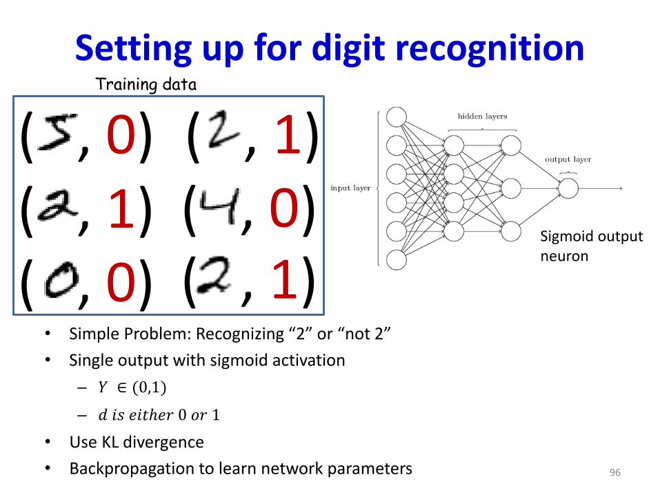
Setting up for digit recognition

• Simple Problem: Recognizing “2” or “not 2”

• Single output with sigmoid activation

– 𝑌 ∈ (0,1)

– 𝑑 𝑖𝑠 𝑒𝑖𝑡ℎ𝑒𝑟 0 𝑜𝑟 1

• Use KL divergence

• Backpropagation to learn network parameters 96

( , 0)( , 1)( , 0)

( , 1)( , 0)( , 1)

Training data

Sigmoid outputneuron

Recognizing the digit

• More complex problem: Recognizing digit

• Network with 10 (or 11) outputs

– First ten outputs correspond to the ten digits

• Optional 11th is for none of the above

• Softmax output layer:

– Ideal output: One of the outputs goes to 1, the others go to 0

• Backpropagation with KL divergence to learn network 97

( , 0)

( , 1)

( , 0)

( , 1)

( , 0)

( , 1)

Training data

Y1 Y2 Y3 Y4 Y0

Issues and Challenges

• What does it learn?• Speed

– Will not address this

• Does it do what we want it to do?

• Next class: – Variations of nnets

• MLP, Convolution, recurrence

– Nnets for various tasks• Image recognition, speech recognition, signal enhancement,

modelling language..

18797/11755 98

Documents

Neural Networks - cs.cmu.edubhiksha/courses/mlsp.fall2017/lectures/lec... · Neural Network 18797/11755 15. ... •A multi-layer perceptron is a universal function approximator