Embed Size (px)
Citation preview

Machine Learning for Vision:
Random Decision Forests and
Deep Neural Networks Kari Pulli VP Computational Imaging Light

Material sources
A. Criminisi & J. Shotton: Decision Forests Tutorial http://research.microsoft.com/en-us/projects/decisionforests/
J. Shotton et al. (CVPR11): Real-Time Human Pose Recognition in Parts from a Single Depth Image
http://research.microsoft.com/apps/pubs/?id=145347 Geoffrey Hinton: Neural Networks for Machine Learning
https://www.coursera.org/course/neuralnets Andrew Ng: Machine Learning
https://www.coursera.org/course/ml Rob Fergus: Deep Learning for Computer Vision
http://media.nips.cc/Conferences/2013/Video/Tutorial1A.pdf https://www.youtube.com/watch?v=qgx57X0fBdA

Andrew Ng
x1
x2
Supervised Learning

Andrew Ng
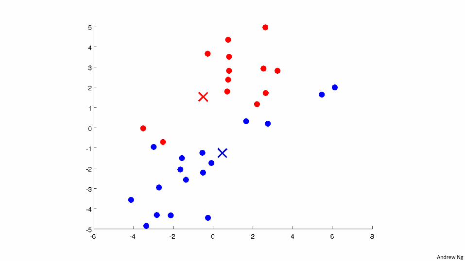
Unsupervised Learning
x1
x2

Andrew Ng
Clustering K-‐means algorithm
Machine Learning

Andrew Ng

Andrew Ng

Andrew Ng

Andrew Ng
Andrew Ng

Andrew Ng

Andrew Ng

Andrew Ng

Decision Forests
for computer vision and medical image analysis
A. Criminisi, J. Shotton and E. Konukoglu
h"p://research.microso/.com/projects/decisionforests

Decision trees and decision forests
A forest is an ensemble of trees. The trees are all slightly different from one another.
terminal (leaf) node
internal (split) node
root node 0
1 2
3 4 5 6
7 8 9 10 11 12 13 14
A general tree structure
Is top part blue?
Is bo"om part green?
Is bo"om part blue?
false
true
A decision tree

Input test point Split the data at node
Decision tree testing (runtime)
Input data in feature space


How to split the data?
Binary tree? Ternary? How big a tree?
Decision tree training (off-line) Input training data
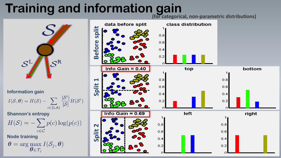
Training and information gain
Before sp
lit
Information gain
Shannon’s entropy
Node training
(for categorical, non-‐parametric distribuHons)
Split 1
Split 2

The weak learner model Node weak learner
Node test params
Splitting data at node j
With a generic line in homog. coordinates.
Weak learner: axis aligned Weak learner: oriented line Weak learner: conic section
Examples of weak learners
Feature response for 2D example.
Feature response for 2D example. With a matrix representing a conic.
Feature response for 2D example. With or

The prediction model What do we do at the leaf?
leaf leaf
leaf
Prediction model: probabilistic

How many trees? How different? How to fuse their outputs?
Decision forest training (off-line)
… …

Decision forest model: the randomness model
1) Bagging (randomizing the training set)
The full training set
The randomly sampled subset of training data made available for the tree t
Forest training
Efficient training

Decision forest model: the randomness model
The full set of all possible node test parameters
For each node the set of randomly sampled features
Randomness control parameter. For no randomness and maximum tree correlaSon. For max randomness and minimum tree correlaSon.
2) Randomized node optimization (RNO)
Small value of ; little tree correlation. Large value of ; large tree correlation.
The effect of
Node weak learner
Node test params
Node training

Classification forest: the ensemble model
Tree t=1 t=2 t=3
Forest output probability
The ensemble model

Training different trees in the forest
TesSng different trees in the forest
(2 videos in this page)
Classification forest: effect of the weak learner model
Parameters: T=200, D=2, weak learner = aligned, leaf model = probabilisHc
• “Accuracy of predicSon”
• “Quality of confidence”
• “GeneralizaSon”
Three concepts to keep in mind:
Training points

Training different trees in the forest
TesSng different trees in the forest
Classification forest: effect of the weak learner model
Parameters: T=200, D=2, weak learner = linear, leaf model = probabilisHc (2 videos in this page)
Training points

Classification forest: effect of the weak learner model Training different trees in the forest
TesSng different trees in the forest
Parameters: T=200, D=2, weak learner = conic, leaf model = probabilisHc (2 videos in this page)
Training points

Classification forest: with >2 classes Training different trees in the forest
TesSng different trees in the forest
Parameters: T=200, D=3, weak learner = conic, leaf model = probabilisHc (2 videos in this page)
Training points


Classification forest: effect of tree depth
max tree depth, D overfi\ng underfi\ng
T=200, D=3, w. l. = conic T=200, D=6, w. l. = conic T=200, D=15, w. l. = conic
Predictor model = prob. (3 videos in this page)
Training points: 4-‐class mixed

Jamie Shotton, Andrew Fitzgibbon, Mat Cook, Toby Sharp, Mark Finocchio, Richard Moore,
Alex Kipman, Andrew Blake
CVPR 2011

right elbow
right hand left shoulder neck

¡ No temporal informaSon § frame-‐by-‐frame
¡ Local pose esSmate of parts
§ each pixel & each body joint treated independently
¡ Very fast § simple depth image features § parallel decision forest classifier

infer body parts per pixel cluster pixels to
hypothesize body joint positions
capture depth image & remove bg
fit model & track skeleton

Train invariance to:
Record mocap 500k frames
distilled to 100k poses
Retarget to several models
Render (depth, body parts) pairs
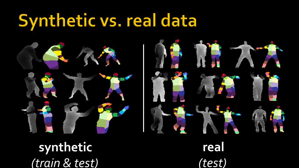
synthetic (train & test)
real (test)

¡ Depth comparisons § very fast to compute
input depth image
x Δ
x Δ
x Δ x
Δ
x Δ
x Δ image depth
image coordinate
offset depth feature
response
Background pixels d = large constant
scales inversely with depth
f(I, x) = dI(x)� dI(x+�)
� = v/dI(x)

depth 1 depth 2 depth 3 depth 4 depth 5 depth 6 depth 7 depth 8 depth 9 depth 10 depth 11 depth 12 depth 13 depth 14 depth 15 depth 16 depth 17 depth 18
input depth ground truth parts inferred parts (soft)

30%
35%
40%
45%
50%
55%
60%
65%
8 12 16 20
Ave
rage
per-‐class
accu
racy
Depth of trees 30%
35%
40%
45%
50%
55%
60%
65%
5 10 15 20 Depth of trees
synthetic test data real test data

ground truth
1 tree 3 trees 6 trees inferred body parts (most likely)
40%
45%
50%
55%
1 2 3 4 5 6
Ave
rage
per-‐class
Number of trees

front view top view side view
input depth inferred body parts
inferred joint positions no tracking or smoothing

front view top view side view
input depth inferred body parts
inferred joint positions no tracking or smoothing

¡ Use… § 3D joint hypotheses § kinemaSc constraints § temporal coherence
¡ … to give
§ full skeleton § higher accuracy § invisible joints § mulS-‐player
4. track skeleton
1
2
3

Feed-forward neural networks • These are the most common type of
neural network in practice – The first layer is the input
and the last layer is the output. – If there is more than one hidden layer,
we call them “deep” neural networks. – Hidden layers learn complex features,
the outputs are learned in terms of those features.
hidden units
output units
input units

Linear neurons
• These are simple but computationally limited
ii
iwxby ∑+=output
bias
index over input connections
i input th
i th weight on
input

Sigmoid neurons
• These give a real-valued output that is a smooth and bounded function of their total input. – They have nice
derivatives which make learning easy
y = 1
1+ e−z
0.5
0 0
1
z
y
z = b+ xii∑ wi
∂z∂wi
= xi∂z∂xi
= widydz
= y (1− y)

Finding weights with backpropagation • There is a big difference between the
forward and backward passes.
• In the forward pass we use squashing functions to prevent the activity vectors from exploding.
• The backward pass, is completely linear. – The forward pass determines the slope
of the linear function used for backpropagating through each neuron.

Backpropagating dE/dy yjj
yii
z j
zj = yii∑ wij
wij
• Find squared error • Propagate error to the
layer below • Compute error
derivative w.r.t. weights • Repeat
y = 1
1+ e−z
Ej =12 (yj − t j )
2

Backpropagating dE/dy
∂E∂zj
=dyjdzj
∂E∂yj
yjj
yii
z jwij
Ej =12 (yj − t j )
2
Propagate error across non-linearity
zj = yii∑ wij
y = 1
1+ e−z

Backpropagating dE/dy
∂E∂zj
=dyjdzj
∂E∂yj
= yj (1− yj )∂E∂yj
yjj
yii
z jwij
Ej =12 (yj − t j )
2
dydz
= y (1− y)
∂E∂y j
= yj − t j
Propagate error across non-linearity
zj = yii∑ wij
y = 1
1+ e−z

∂E∂zj
=dyjdzj
∂E∂yj
= yj (1− yj )∂E∂yj
∂E∂y j
= yj − t jBackpropagating dE/dy
yjj
yii
z j
∂E∂yi
=dzjdyi
∂E∂zjj
∑
wij
Ej =12 (yj − t j )
2
dydz
= y (1− y)
Propagate error to the next activation across connections
zj = yii∑ wij
y = 1
1+ e−z

∂E∂y j
= yj − t jBackpropagating dE/dy
yjj
yii
z j
∂E∂yi
=dzjdyi
∂E∂z jj
∑ = wij∂E∂z jj
∑
wij
Ej =12 (yj − t j )
2
dydz
= y (1− y)
Propagate error to the next activation across connections
zj = yii∑ wij
y = 1
1+ e−z
∂E∂zj
=dyjdzj
∂E∂yj
= yj (1− yj )∂E∂yj

∂E∂zj
=dyjdzj
∂E∂yj
= yj (1− yj )∂E∂yj
∂E∂yi
=dzjdyi
∂E∂z jj
∑ = wij∂E∂z jj
∑
∂E∂y j
= yj − t jBackpropagating dE/dy
yjj
yii
z j
∂E∂wij
=∂zj∂wij
∂E∂zj
wij
Ej =12 (yj − t j )
2
dydz
= y (1− y) Error gradient w.r.t. weights
zj = yii∑ wij
y = 1
1+ e−z

∂E∂yi
=dzjdyi
∂E∂z jj
∑ = wij∂E∂z jj
∑
∂E∂y j
= yj − t j
∂E∂zj
=dyjdzj
∂E∂yj
= yj (1− yj )∂E∂yj
Backpropagating dE/dy yjj
yii
z j
∂E∂wij
=∂z j∂wij
∂E∂z j
= yi∂E∂z j
wij
Ej =12 (yj − t j )
2
dydz
= y (1− y) Error gradient w.r.t. weights
zj = yii∑ wij
y = 1
1+ e−z

∂E∂zj
=dyjdzj
∂E∂yj
= yj (1− yj )∂E∂yj
∂E∂yi
=dzjdyi
∂E∂z jj
∑ = wij∂E∂z jj
∑
∂E∂y j
= yj − t jBackpropagating dE/dy
yjj
yii
∂E∂wij
=∂z j∂wij
∂E∂z j
= yi∂E∂z j
wij
Ej =12 (yj − t j )
2
y = 1
1+ e−zdydz
= y (1− y)
zj = yii∑ wij
z j

Converting error derivatives into a learning procedure
• The backpropagation algorithm is an efficient way of computing the error derivative dE/dw for every weight on a single training case.
• To get a fully specified learning procedure, we still need to make a lot of other decisions about how to use these error derivatives: – Optimization issues: How do we use the error derivatives on
individual cases to discover a good set of weights? – Generalization issues: How do we ensure that the learned weights
work well for cases we did not see during training?
Andrew Ng
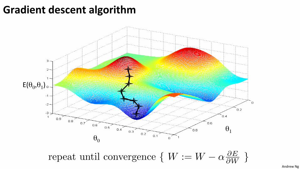
θ1θ0
E(θ0,θ1)
Gradient descent algorithm
repeat until convergence { W := W � ↵ @E@W }

Andrew Ng
θ0
θ1
E(θ0,θ1)
Gradient descent algorithm
repeat until convergence { W := W � ↵ @E@W }

Overfitting: The downside of using powerful models • The training data contains information about the regularities in the
mapping from input to output. But it also contains two types of noise. – The target values may be unreliable – There is sampling error:
accidental regularities just because of the particular training cases that were chosen.
• When we fit the model, it cannot tell which regularities are real and which are caused by sampling error. – So it fits both kinds of regularity. – If the model is very flexible it can model the sampling error really
well. This is a disaster.

Andrew Ng
Example: LogisSc regression
( = sigmoid funcSon)
x1
x2
x1
x2
x1
x2

Preventing overfitting
• Approach 1: Get more data! – almost always the best bet if you
have enough compute power to train on more data
• Approach 2: Use a model that has the right capacity: – enough to fit the true regularities. – not enough to also fit spurious
regularities (if they are weaker)
• Approach 3: Average many different models. – use models with different forms
• Approach 4: (Bayesian) Use a single neural network architecture, but average the predictions made by many different weight vectors. – train the model on different
subsets of the training data (this is called “bagging”)

Some ways to limit the capacity of a neural net
• The capacity can be controlled in many ways: – Architecture: Limit the number of hidden layers and the number
of units per layer. – Early stopping: Start with small weights and stop the learning
before it overfits. – Weight-decay: Penalize large weights using penalties or
constraints on their squared values (L2 penalty) or absolute values (L1 penalty).
– Noise: Add noise to the weights or the activities. • Typically, a combination of several of these methods is used.

Small Model vs. Big Model + Regularize
Small model Big model Big model + regularize

Cross-validation for choosing meta parameters
• Divide the total dataset into three subsets: – Training data is used for learning the parameters of the model. – Validation data is not used for learning but is used for deciding
what settings of the meta parameters work best. – Test data is used to
get a final, unbiased estimate of how well the network works.
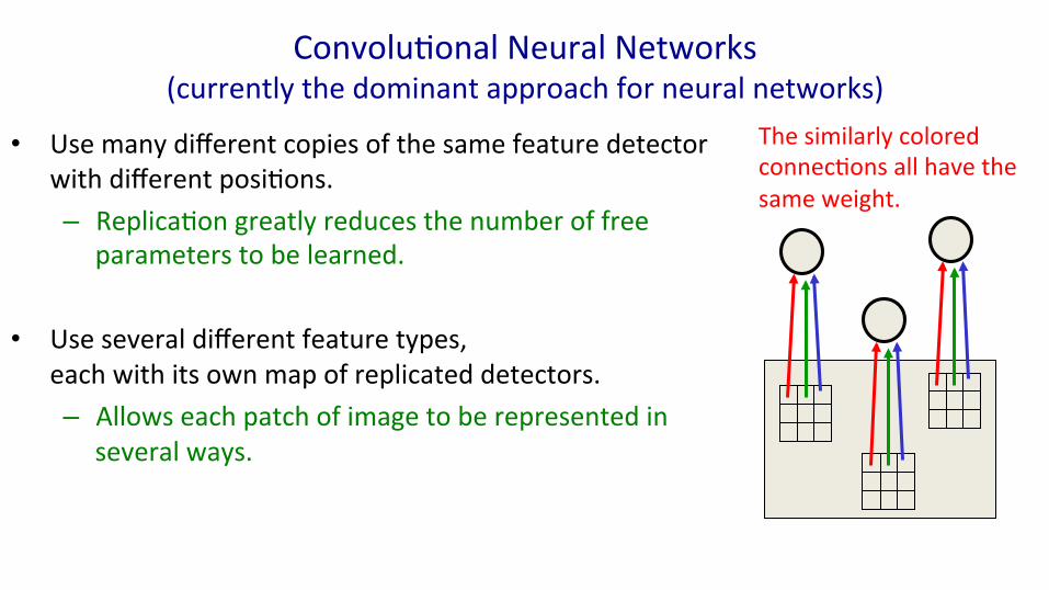
ConvoluSonal Neural Networks (currently the dominant approach for neural networks)
• Use many different copies of the same feature detector with different posiSons. – ReplicaSon greatly reduces the number of free
parameters to be learned.
• Use several different feature types, each with its own map of replicated detectors. – Allows each patch of image to be represented in
several ways.
The similarly colored connecSons all have the same weight.
Le Net
• Yann LeCun and his collaborators developed a really good recognizer for handwrihen digits by using backpropagaSon in a feedforward net with: – Many hidden layers – Many maps of replicated convoluSon units in each layer – Pooling of the outputs of nearby replicated units – A wide input can cope with several digits at once even if they overlap
• This net was used for reading ~10% of the checks in North America. • Look the impressive demos of LENET at hhp://yann.lecun.com


The architecture of LeNet5

Pooling the outputs of replicated feature detectors • Get a small amount of translational invariance at each level by
averaging four neighboring outputs to give a single output. – This reduces the number of inputs to the next layer of
feature extraction. – Taking the maximum of the four works slightly better.
• Problem: After several levels of pooling, we have lost information about the precise positions of things.

The architecture of LeNet5


The 82 errors made by LeNet5
Notice that most of the errors are cases that people find quite easy.
The human error rate is probably 20 to 30 errors but nobody has had the patience to measure it.
Test set size is 10000.

The brute force approach
• LeNet uses knowledge about the invariances to design: – the local connectivity – the weight-sharing – the pooling.
• This achieves about 80 errors.
• Ciresan et al. (2010) inject knowledge of invariances by creating a huge amount of carefully designed extra training data: – For each training image, they
produce many new training examples by applying many different transformations.
– They can then train a large, deep, dumb net on a GPU without much overfitting.
• They achieve about 35 errors.

From hand-‐wrihen digits to 3-‐D objects
• Recognizing real objects in color photographs downloaded from the web is much more complicated than recognizing hand-‐wrihen digits: – Hundred Smes as many classes (1000 vs. 10) – Hundred Smes as many pixels (256 x 256 color vs. 28 x 28 gray) – Two dimensional image of three-‐dimensional scene. – Cluhered scenes requiring segmentaSon – MulSple objects in each image.
• Will the same type of convoluSonal neural network work?

The ILSVRC-2012 competition on ImageNet
• The dataset has 1.2 million high-resolution training images. • The classification task:
– Get the “correct” class in your top 5 bets. There are 1000 classes.
• The localization task: – For each bet, put a box around the object.
Your box must have at least 50% overlap with the correct box.

Examples from the test set (with the network’s guesses)

Tricks that significantly improve generalizaSon
• Train on random 224x224 patches from the 256x256 images to get more data. Also use left-right reflections of the images. • At test time, combine the
opinions from ten different patches: The four 224x224 corner patches plus the central 224x224 patch plus the reflections of those five patches.
• Use “dropout” to regularize the weights in the globally connected layers (which contain most of the parameters). – Dropout means that half of
the hidden units in a layer are randomly removed for each training example.
– This stops hidden units from relying too much on other hidden units.
Auto-‐Encoders

Restricted Boltzmann Machines
• Simple recursive neural net – Only one layer of hidden
units. – No connections between
hidden units. • Idea:
– The hidden layer should “auto-encode” the input.
p(hj = 1) =1
1+ e−(bj+ viwij)
i∈vis∑
hidden
visible i
j

Contrastive divergence to train an RBM
t = 0 t = 1
Δwij = ε ( <vihj>0 − <vihj>
1)
Start with a training vector on the visible units.
Update all the hidden units in parallel.
Update all the visible units in parallel to get a “reconstruction”.
Update the hidden units again. reconstruction data
<vihj>0 <vihj>
1
i
j
i
j

Explanation
t = 0 t = 1
Δwij = ε ( <vihj>0 − <vihj>
1)
Ideally, hidden layers re-generate the input.
If that’s not the case, the hidden layers generate something else.
Change the weights so that this wouldn’t happen. reconstruction data
<vihj>0 <vihj>
1
i
j
i
j

The weights of the 50 feature detectors
We start with small random weights to break symmetry


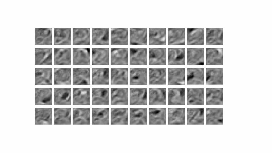


The final 50 x 256 weights: Each neuron grabs a different feature

Reconstruction from activated binary features Data
Reconstruction from activated binary features Data
How well can we reconstruct digit images from the binary feature activations?
New test image from the digit class that the model was trained on
Image from an unfamiliar digit class The network tries to see every image as a 2.

Krizhevsky’s deep autoencoder
1024 1024 1024
8192
4096
2048
1024
512
256-bit binary code The encoder has about 67,000,000 parameters.

Reconstructions of 32x32 color images from 256-bit codes

retrieved using 256 bit codes
retrieved using Euclidean distance in pixel intensity space

retrieved using 256 bit codes
retrieved using Euclidean distance in pixel intensity space


![NBDT: Neural-Backed Decision Trees · trees [4,5,15]. Work converting from decision trees to neural networks also dates back three decades [14,17,6,7]. Like distillation [12], these](https://img.pdfslide.us/doc/110x75/5f81d65184cf6705116a1725/nbdt-neural-backed-decision-trees-trees-4515-work-converting-from-decision.jpg)


![arXiv:2005.05131v1 [cs.AI] 11 May 2020Multi-Layered Artificial Neural Networks, Decision Trees, Support Vector Machines, K-Nearest Neighbor, Random Forest, Gradient Boosted Trees](https://img.pdfslide.us/doc/110x75/5ec51e86848dae130f38728f/arxiv200505131v1-csai-11-may-2020-multi-layered-artiicial-neural-networks.jpg)