Embed Size (px)
Citation preview
Neural Network Weight Selection Using GeneticAlgorithms
David Montana
presented by:
Carl Fink, Hongyi Chen, Jack Cheng,
Xinglong Li, Bruce Lin, Chongjie Zhang
April 12, 2005
1
Neural Networks
Neural networks generally consist of five components.
• A directed graph known as the network topology whose nodes
represent the neurodes (or processing elements) and whose arcs
represent the connections.
• A state variable associated with each neurode.
• A real-valued weight associated with each connection.
• A real-valued bias associated with each neurode.
• A transfer function f for each neurode such that the state of the
neurode is f(ωixi − β).
2
Genetic Algorithms
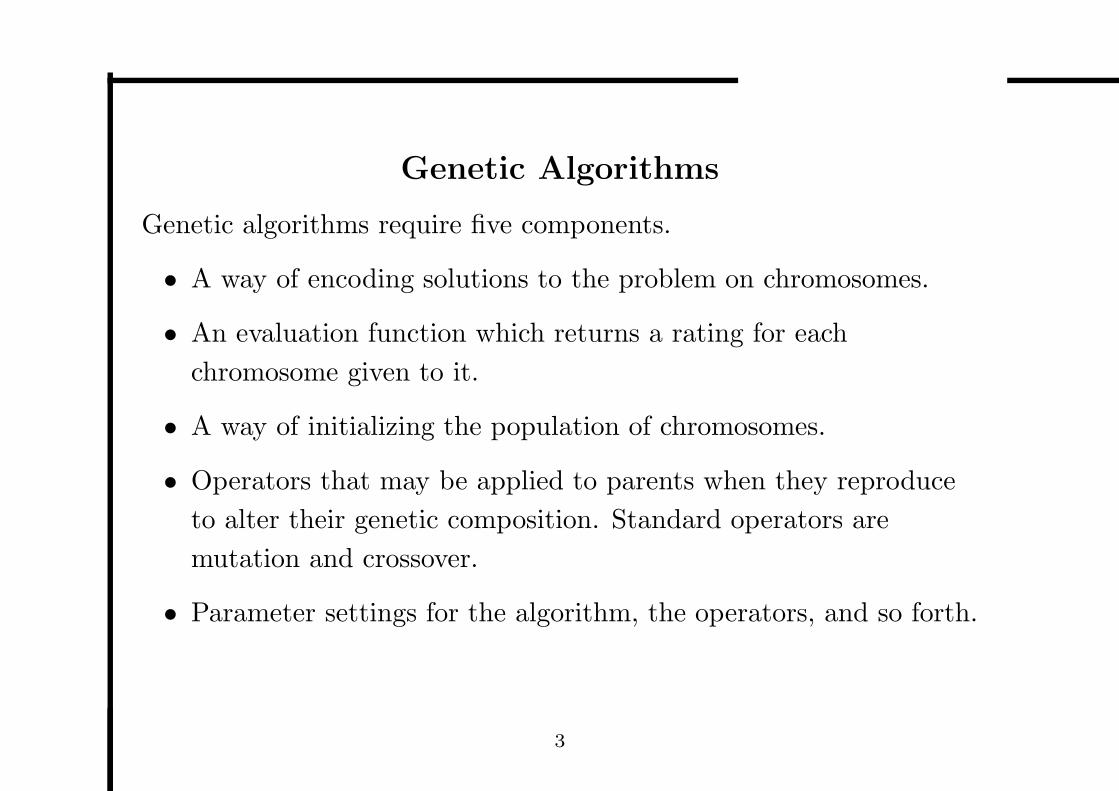
Genetic algorithms require five components.
• A way of encoding solutions to the problem on chromosomes.
• An evaluation function which returns a rating for each
chromosome given to it.
• A way of initializing the population of chromosomes.
• Operators that may be applied to parents when they reproduce
to alter their genetic composition. Standard operators are
mutation and crossover.
• Parameter settings for the algorithm, the operators, and so forth.
3
Genetic Algorithms
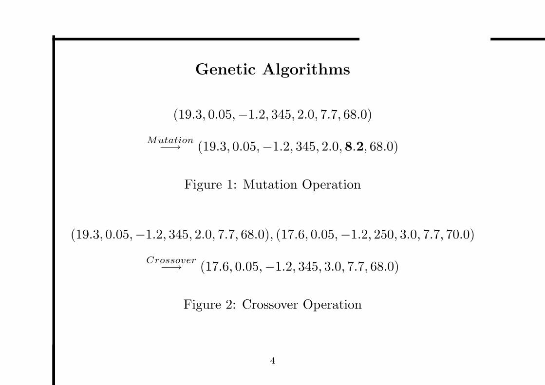
(19.3, 0.05,−1.2, 345, 2.0, 7.7, 68.0)
Mutation−→ (19.3, 0.05,−1.2, 345, 2.0,8.2, 68.0)
Figure 1: Mutation Operation
(19.3, 0.05,−1.2, 345, 2.0, 7.7, 68.0), (17.6, 0.05,−1.2, 250, 3.0, 7.7, 70.0)
Crossover−→ (17.6, 0.05,−1.2, 345, 3.0, 7.7, 68.0)
Figure 2: Crossover Operation
4
Genetic Algorithms
Given these five components, a genetic algorithm operates according
to the following steps.
• Initialize the population using the initialization procedure, and
evaluate each member of the initial population.
• Reproduce until a stopping criterion is met.
5
Genetic Algorithms
Reproduction consists of iterations of the following steps.
• Choose one or more parents to reproduce. Selection is stochastic,
but the individuals with the highest evaluations are favored in
the selection.
• Choose a genetic operator and apply it to the parents.
• Evaluate the children and accumulate them into a generation.
After accumulating enough individuals, insert them into the
population, replacing the worst current members of the
population.
6
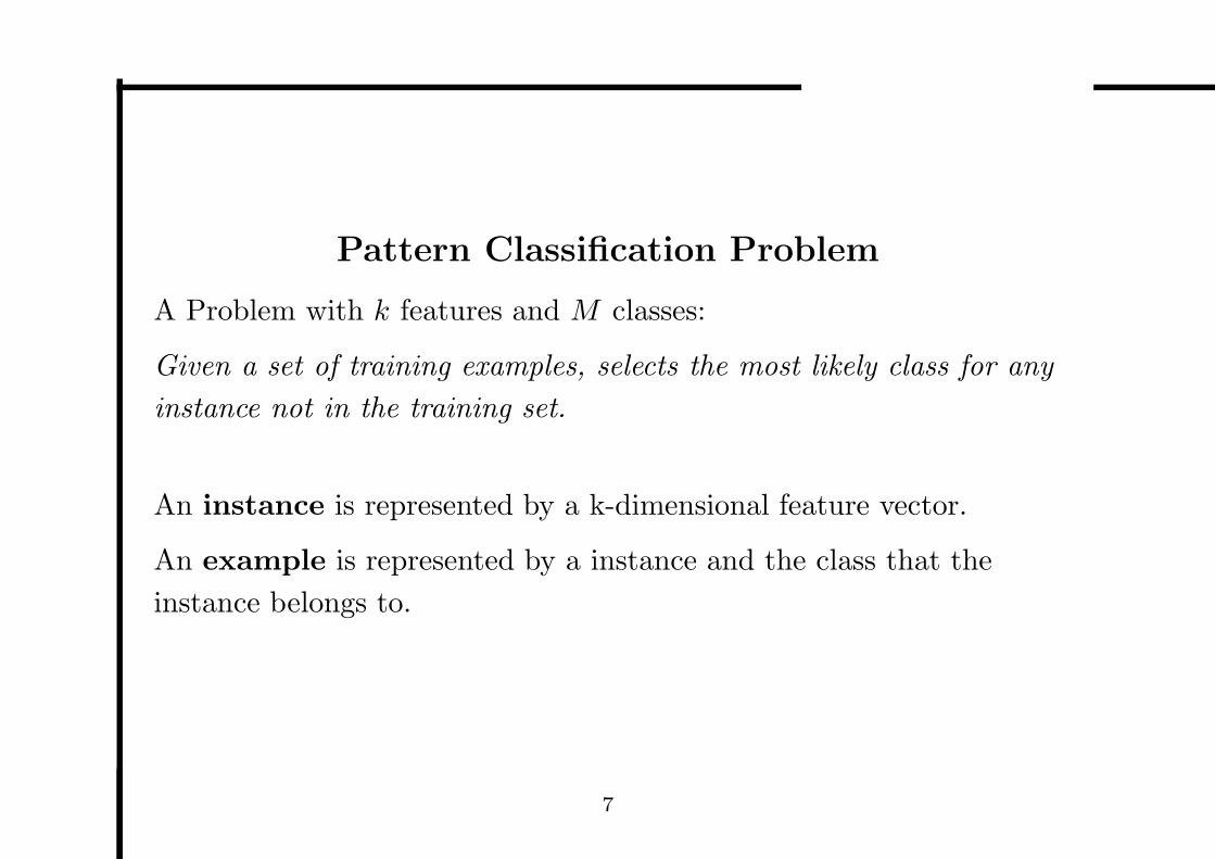
Pattern Classification Problem
A Problem with k features and M classes:
Given a set of training examples, selects the most likely class for any
instance not in the training set.
An instance is represented by a k-dimensional feature vector.
An example is represented by a instance and the class that the
instance belongs to.
7
Real Examples
• Handwritten character recognition
• Speech recognition
• Blood cell classification
• . . .
8
Neural Networks
• Sigmoid Feed-forward Neural Network
• Weighted Probabilistic Neural Networks (WPNN)
9
Sigmoid Feed-forward Networks
A feed-forward network
• A directed graph without cycles.
• A multi-layer network
Neurones in each layer (except output layer) are completely
connected to the forward layer.
• Each neuron in the network is a sigmoid unit
10
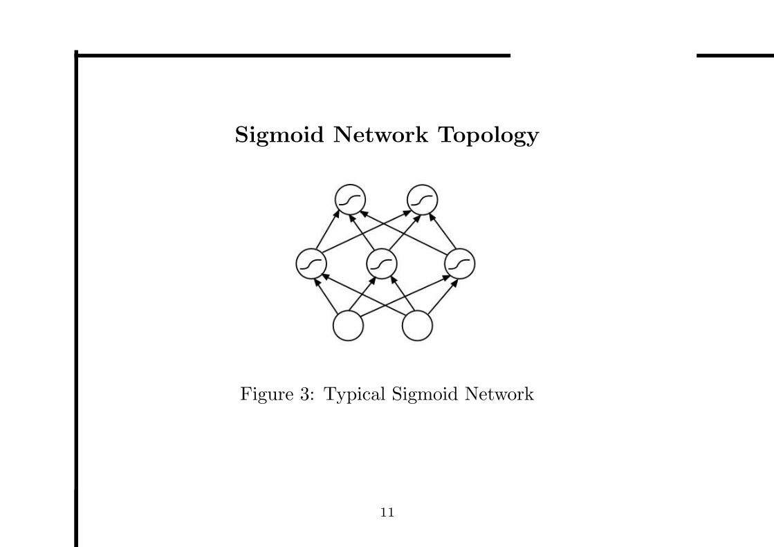
Sigmoid Network Topology
Figure 3: Typical Sigmoid Network
11
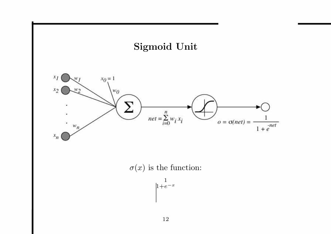
Sigmoid Unit
σ(x) is the function:
11+e−x
12
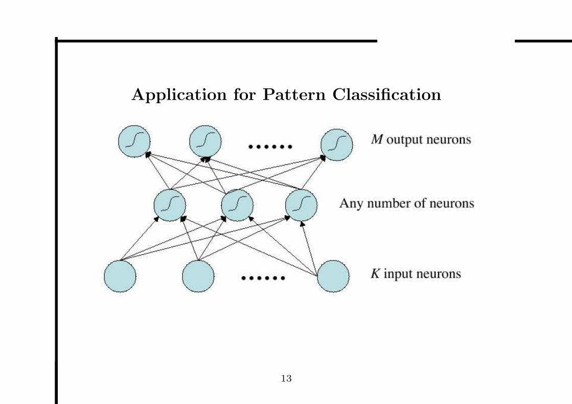
Application for Pattern Classification
13
Application for Pattern Classification (Cont.)
• Representation:
– Input representation: < x1, x2, . . . , xk >
– Class representation: < 1, 0, . . . , 0 > for class 1
• Evaluation Function
The sum of squared errors
• Training Algorithms
– Backpropagation Algorithm
– Genetic Algorithm
14
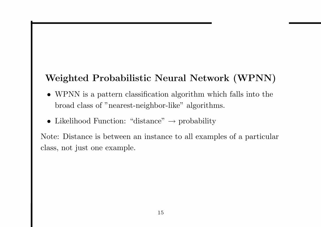
Weighted Probabilistic Neural Network (WPNN)
• WPNN is a pattern classification algorithm which falls into the
broad class of ”nearest-neighbor-like” algorithms.
• Likelihood Function: “distance” → probability
Note: Distance is between an instance to all examples of a particular
class, not just one example.
15
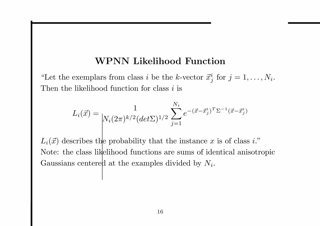
WPNN Likelihood Function
“Let the exemplars from class i be the k-vector ~xij for j = 1, . . . , Ni.
Then the likelihood function for class i is
Li(~x) =1
Ni(2π)k/2(detΣ)1/2
Ni∑
j=1
e−(~x−~xij)
T Σ−1(~x−~xij)
Li(~x) describes the probability that the instance x is of class i.”
Note: the class likelihood functions are sums of identical anisotropic
Gaussians centered at the examples divided by Ni.
16
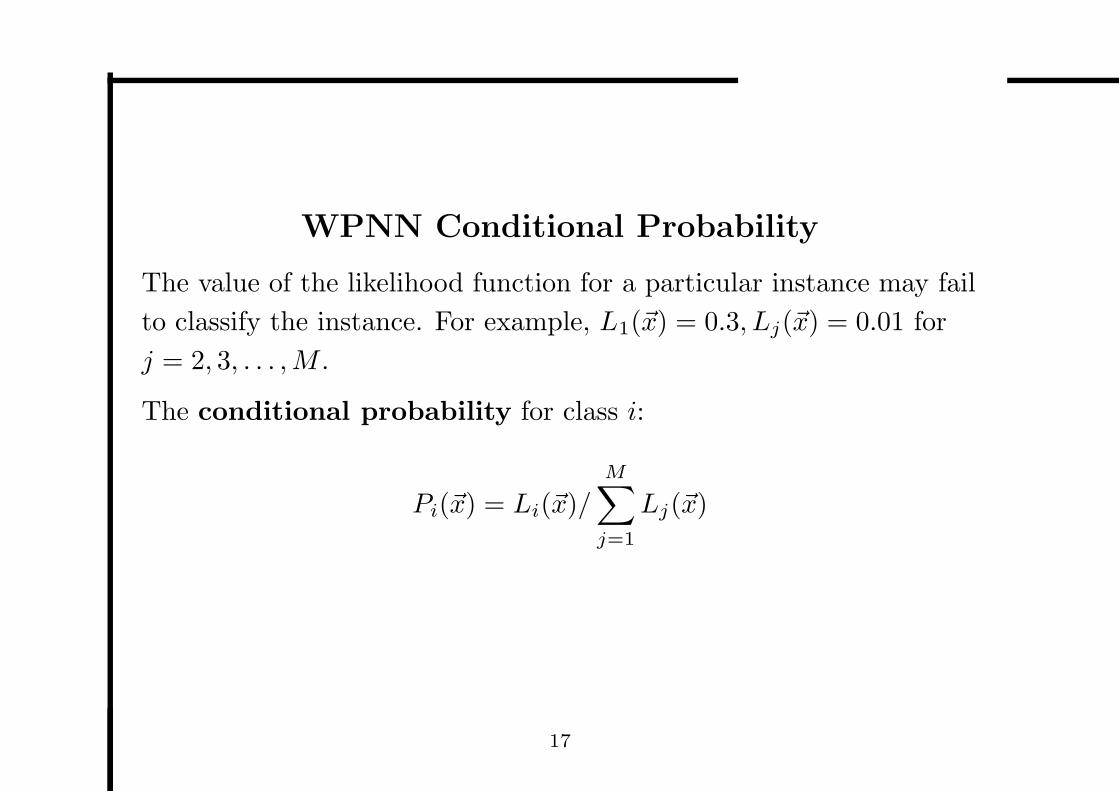
WPNN Conditional Probability
The value of the likelihood function for a particular instance may fail
to classify the instance. For example, L1(~x) = 0.3, Lj(~x) = 0.01 for
j = 2, 3, . . . , M .
The conditional probability for class i:
Pi(~x) = Li(~x)/M∑
j=1
Lj(~x)
17
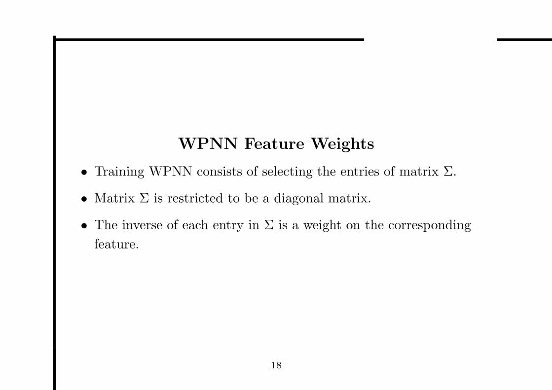
WPNN Feature Weights
• Training WPNN consists of selecting the entries of matrix Σ.
• Matrix Σ is restricted to be a diagonal matrix.
• The inverse of each entry in Σ is a weight on the corresponding
feature.
18
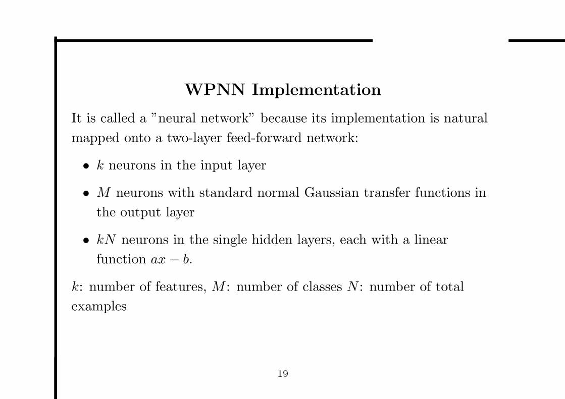
WPNN Implementation
It is called a ”neural network” because its implementation is natural
mapped onto a two-layer feed-forward network:
• k neurons in the input layer
• M neurons with standard normal Gaussian transfer functions in
the output layer
• kN neurons in the single hidden layers, each with a linear
function ax − b.
k: number of features, M : number of classes N : number of total
examples
19
WPNN Implementation (Cont.)
The ((i − 1)k + j)th hidden neuron (i < N, j < k):
1. is connected to the jth input neuron with weight a = 1.0
2. has bias b equal to the value of jth feature of the ith example
3. is connected to the nth output neuron, where n is the class of the
ith exemplar, with weight wj , where wj is the selected feature
weight for the jth feature.
20
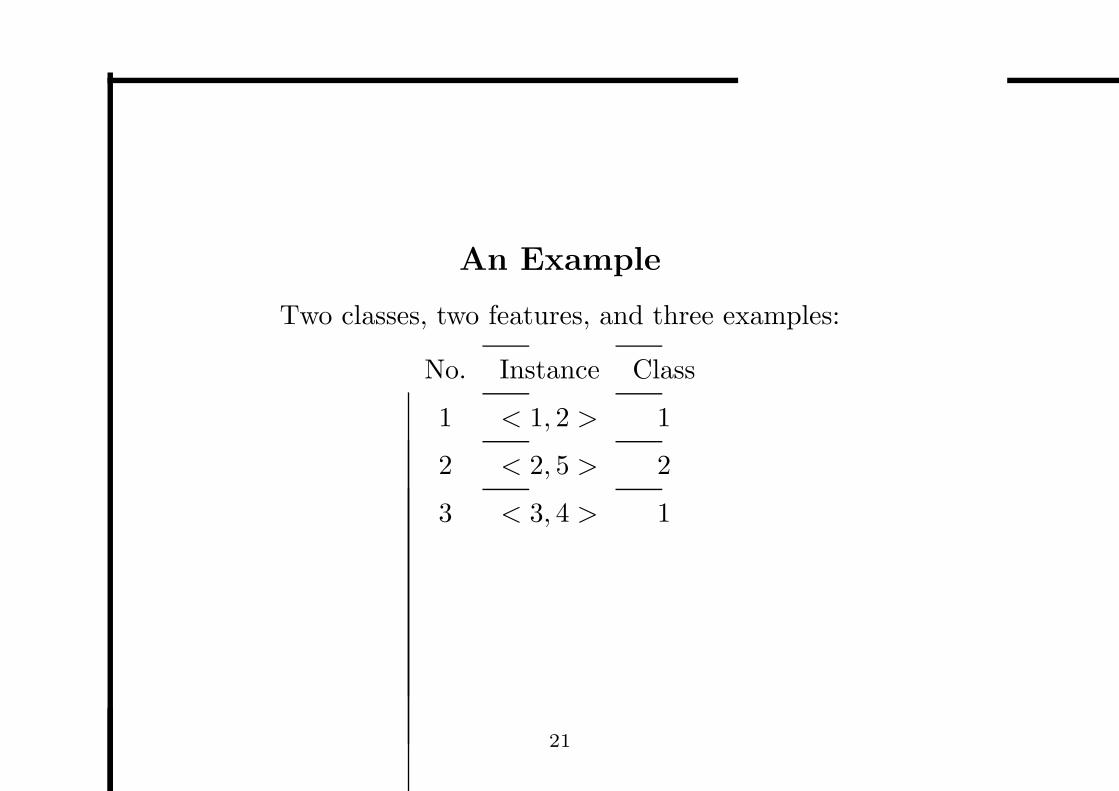
An Example
Two classes, two features, and three examples:
No. Instance Class
1 < 1, 2 > 1
2 < 2, 5 > 2
3 < 3, 4 > 1
21
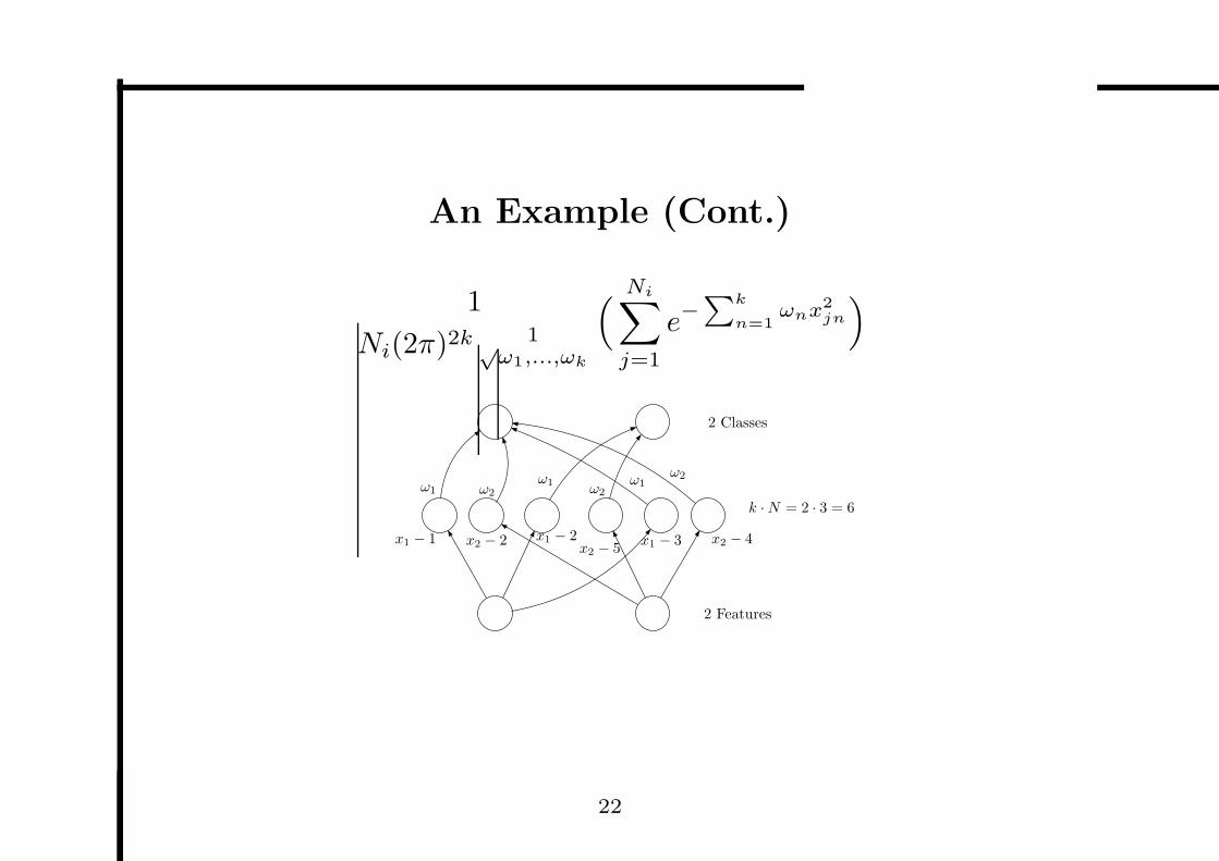
An Example (Cont.)
1
Ni(2π)2k 1√ω1,...,ωk
(
Ni∑
j=1
e−∑
k
n=1ωnx2
jn
)
x1 − 1 x2 − 2 x1 − 2x2 − 5
x1 − 3 x2 − 4
2 Classes
k · N = 2 · 3 = 6
2 Features
ω1 ω2ω1
ω2ω1
ω2
22
Survey of Hybrid Systems
• Supportive combinations
Supportive combinations typically involve using one of these
methods to prepare data for consumption by the other. For
example, using a genetic algorithm to select features for use by
neural network classifiers.
• Collaborative combinations
Collaborative combinations typically involve using the genetic
algorithm to determine the neural network weights or the
topology or learning algorithm.
23
Supportive Combinations
• Using NN to assist GA
• Using GA to assist NN
– Data preparation
– Evolving network parameters and learning rules
– Using GA to explain and analyze NN
• Using GA and NN independently
24
Collaborative Combinations
GA to select weight
Two basic differences between different approaches: architectures
(feedforward sigmoidal, WPNN, cascade-correlation, recurrent
sigmoidal, recurrent linear threshold, feedforward with step functions
and feedback with step functions) and difference in GA itself.
25
Collaborative Combinations
• GA to specify NN topology
– A genotype representation must be devised and an attendant
mapping from genotype to phenotype must be provided.
– There must be a protocol for exposing the phenotype to the
task environment.
– There must be a learning method to fine tune the network
function.
– There must be a fitness measure.
– There must be method for generating new genotypes.
• GA to learn the NN learning algorithm
26
Reasons to apply GA to NN
• Finding the global optima
• For recurrent networks
• For networks with discontinuous functions
• GA can optimize any combination of weights, biases, topology
and transfer functions
• The ability to use arbitrary evaluation function
27
Disadvantage and Solutions
• Excessive computing time
• Solutions:
– Using specialized NN hardware
– Using the best local learning algorithm
– Using parallel implementations of GA
– By finding the best division of labor between the local and
evolutionary learning paradigms to make the best possible use
of training time
28
GA Formulation for Training Sigmoid FFNN
• Problem Formulation
• Initialization
• Genetic Operators
• Fitness Evaluation
• Genetic Parameters
29
Problem Formulation
• Individuals are the NN’s themselves;
• no string encoding
• Topology is fixed, weights are evolved
30
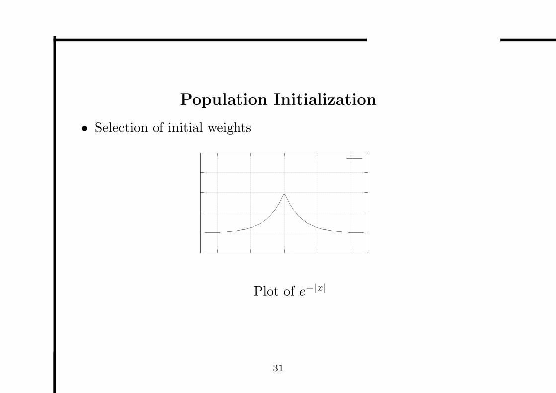
Population Initialization
• Selection of initial weights
Plot of e−|x|
31
Fitness Evaluation
• Sum of Squared Error
E(~ω) ≡ 1/2∑
d∈D
∑
k∈outputs
(tkd − okd)2
32
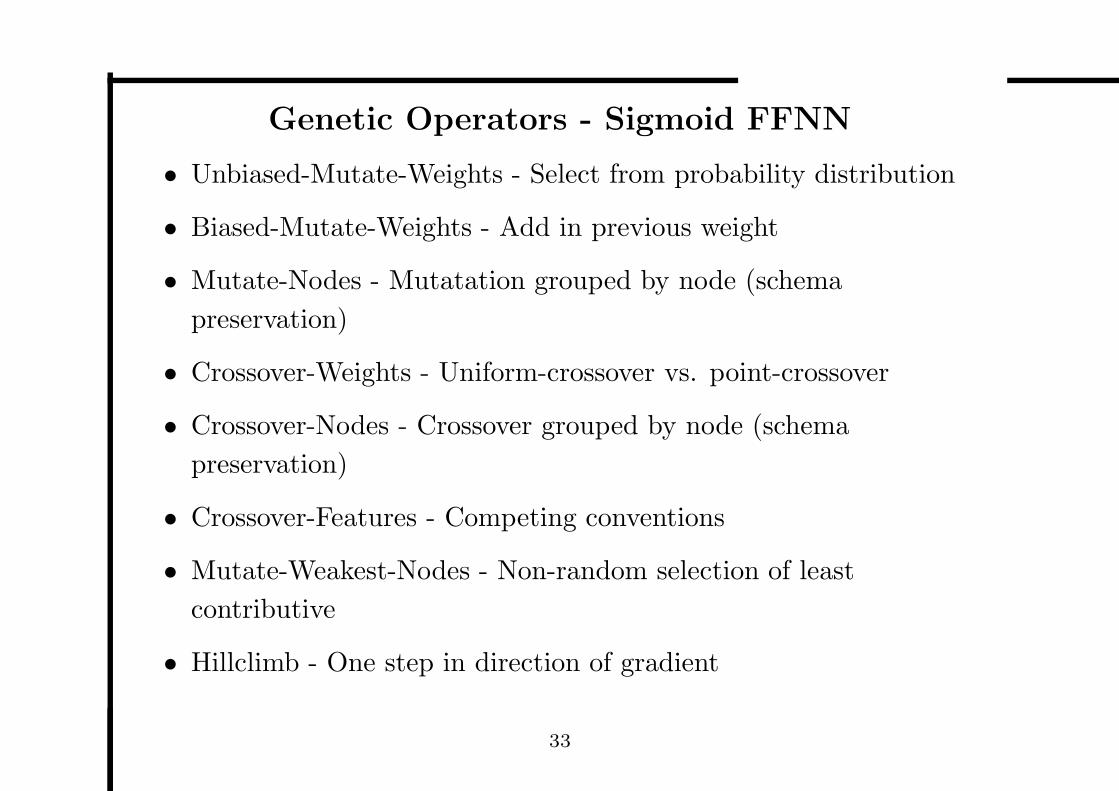
Genetic Operators - Sigmoid FFNN
• Unbiased-Mutate-Weights - Select from probability distribution
• Biased-Mutate-Weights - Add in previous weight
• Mutate-Nodes - Mutatation grouped by node (schema
preservation)
• Crossover-Weights - Uniform-crossover vs. point-crossover
• Crossover-Nodes - Crossover grouped by node (schema
preservation)
• Crossover-Features - Competing conventions
• Mutate-Weakest-Nodes - Non-random selection of least
contributive
• Hillclimb - One step in direction of gradient
33
Parameter Values
• Population-Size: 50
• Generation-Size: 1
• Parent-Scalar: [0.89, 0.93]
34
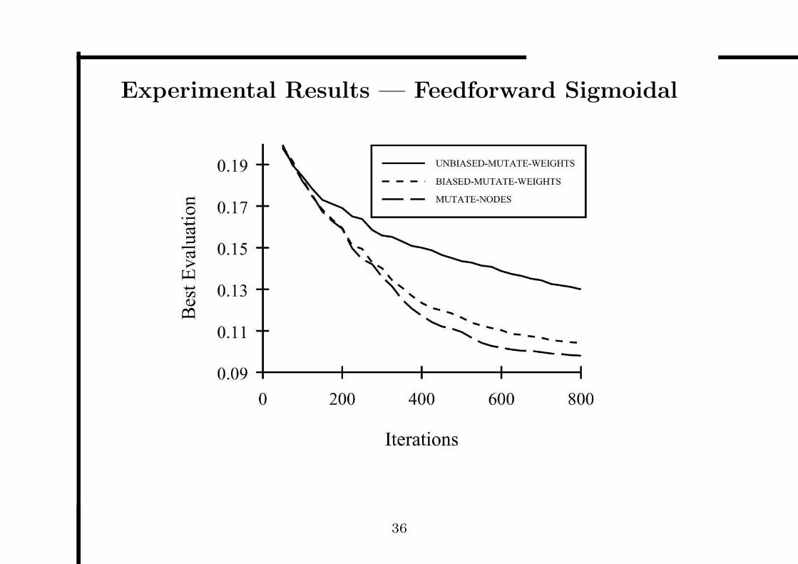
Experimental Results — Feedforward Sigmoidal
First, Comparing the three mutations resulted in a clear order
1. MUTATE-NODES
2. BIASED-MUTATE-WEIGHTS
3. UNBIASED-MUTATE-WEIGHTS
35
Experimental Results — Feedforward Sigmoidal
36
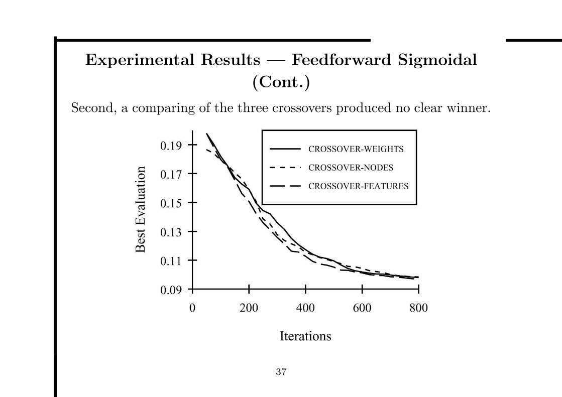
Experimental Results — Feedforward Sigmoidal
(Cont.)
Second, a comparing of the three crossovers produced no clear winner.
37
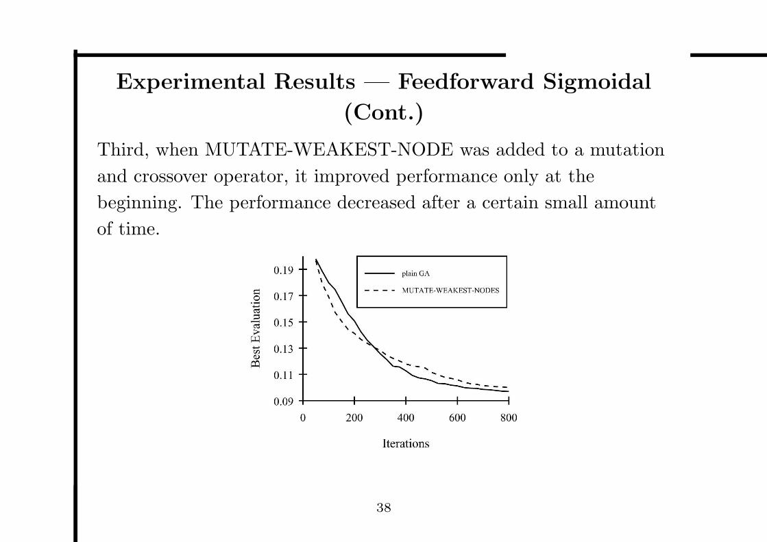
Experimental Results — Feedforward Sigmoidal
(Cont.)
Third, when MUTATE-WEAKEST-NODE was added to a mutation
and crossover operator, it improved performance only at the
beginning. The performance decreased after a certain small amount
of time.
38
Experimental Results — Feedforward Sigmoidal
(Cont.)
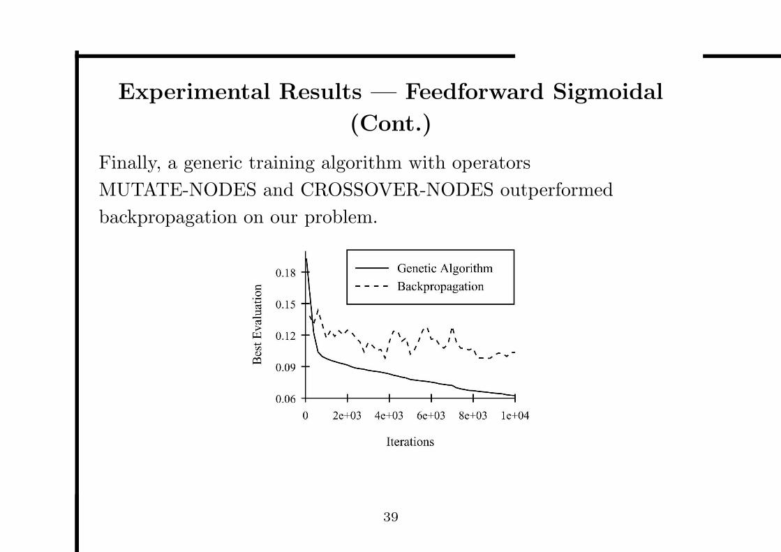
Finally, a generic training algorithm with operators
MUTATE-NODES and CROSSOVER-NODES outperformed
backpropagation on our problem.
39
Experimental Results — Feedforward Sigmoidal
(Cont.)
Backpropagation Algorithm is more computationally efficient than
Genetic Algorithm.
40
Five Components of the genetic algorithm with
WPNN:
Representation
• a ”logarithmic” representation for large dynamic range with
proportional resolution;
• Map: n → Bn−k0
41
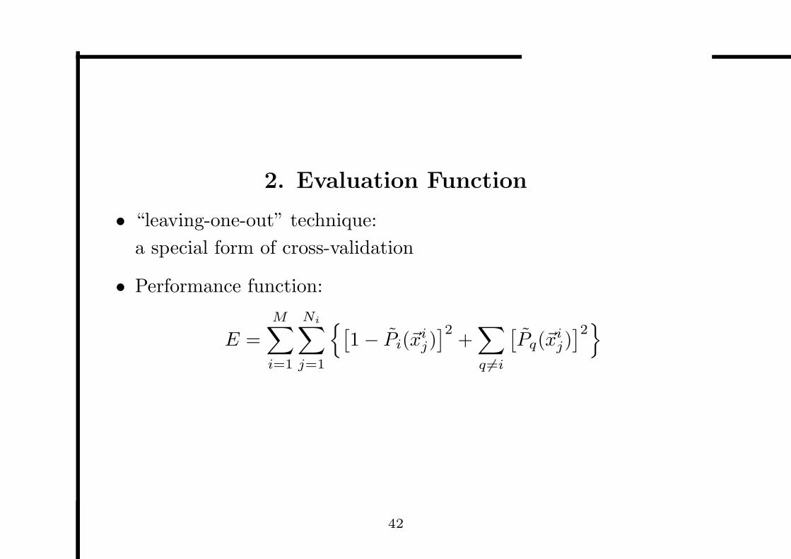
2. Evaluation Function
• “leaving-one-out” technique:
a special form of cross-validation
• Performance function:
E =M∑
i=1
Ni∑
j=1
{
[
1 − P̃i(~xij)
]2+
∑
q 6=i
[
P̃q(~xij)
]2}
42
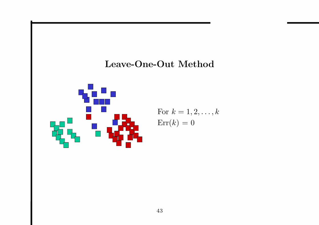
Leave-One-Out Method
For k = 1, 2, . . . , k
Err(k) = 0
43
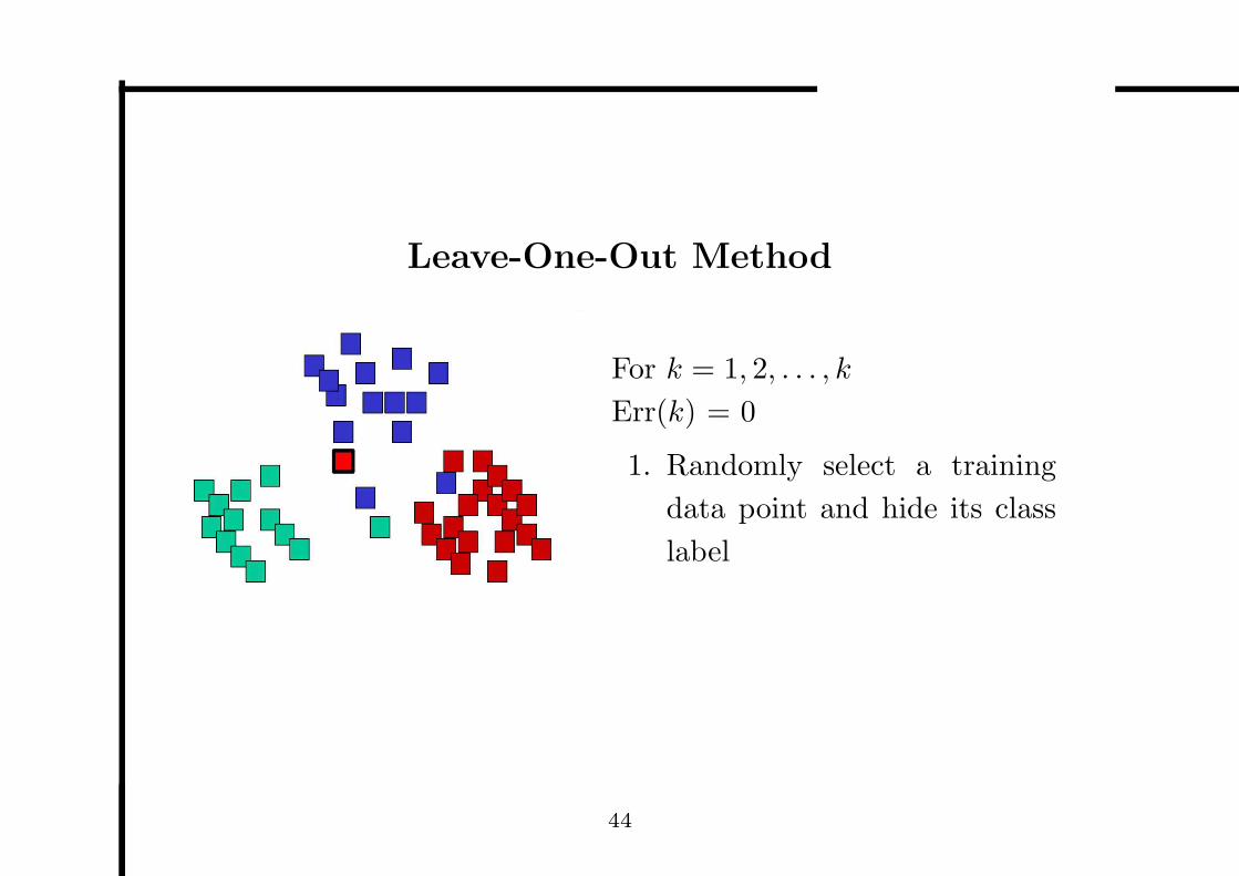
Leave-One-Out Method
For k = 1, 2, . . . , k
Err(k) = 0
1. Randomly select a training
data point and hide its class
label
44
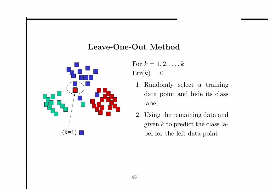
Leave-One-Out Method
For k = 1, 2, . . . , k
Err(k) = 0
1. Randomly select a training
data point and hide its class
label
2. Using the remaining data and
given k to predict the class la-
bel for the left data point
45
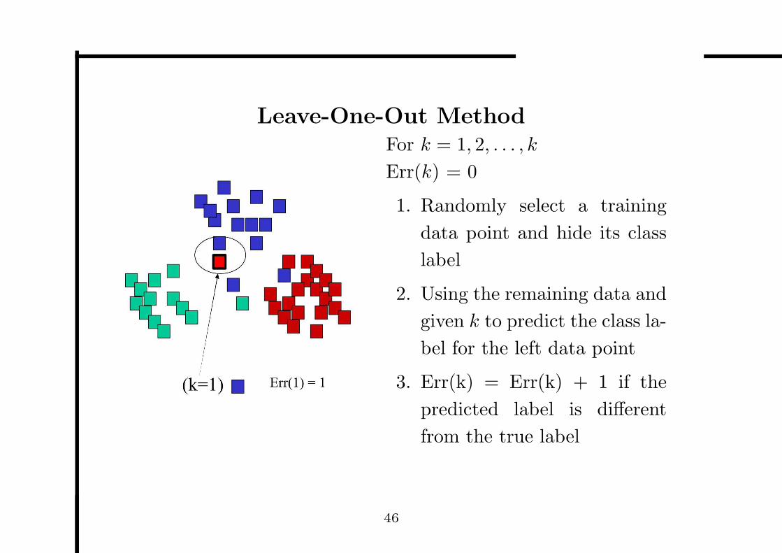
Leave-One-Out MethodFor k = 1, 2, . . . , k
Err(k) = 0
1. Randomly select a training
data point and hide its class
label
2. Using the remaining data and
given k to predict the class la-
bel for the left data point
3. Err(k) = Err(k) + 1 if the
predicted label is different
from the true label
46
Leave-One-Out MethodFor k = 1, 2, . . . , k
Err(k) = 0
1. Randomly select a training
data point and hide its class
label
2. Using the remaining data and
given k to predict the class la-
bel for the left data point
3. Err(k) = Err(k) + 1 if the
predicted label is different
from the true labelRepeat the procedure until all training examples are tested.
47
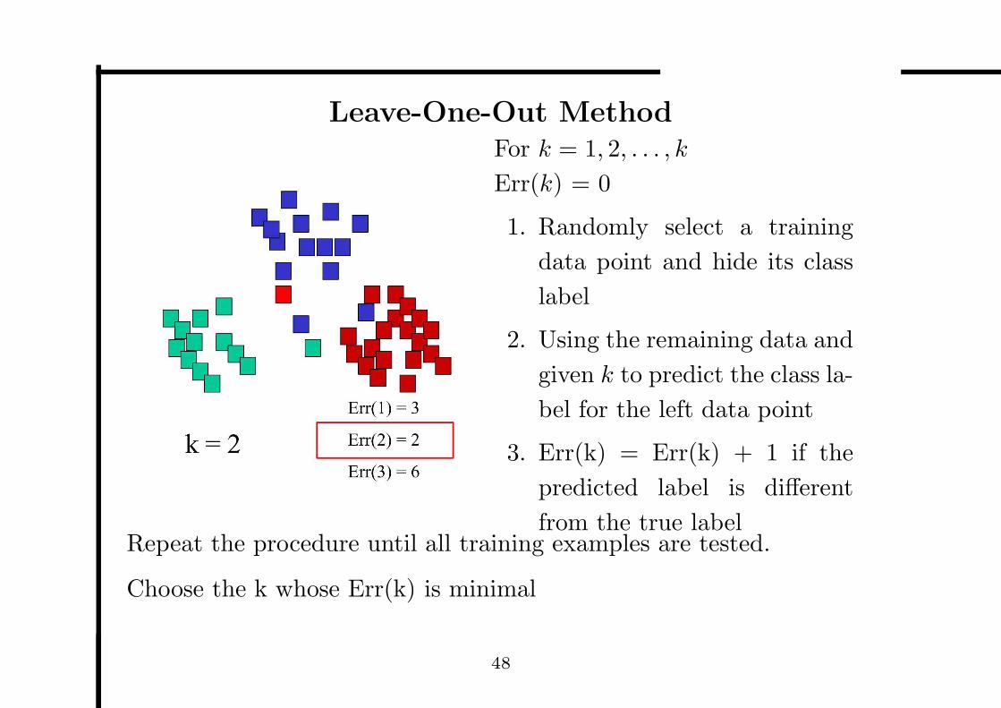
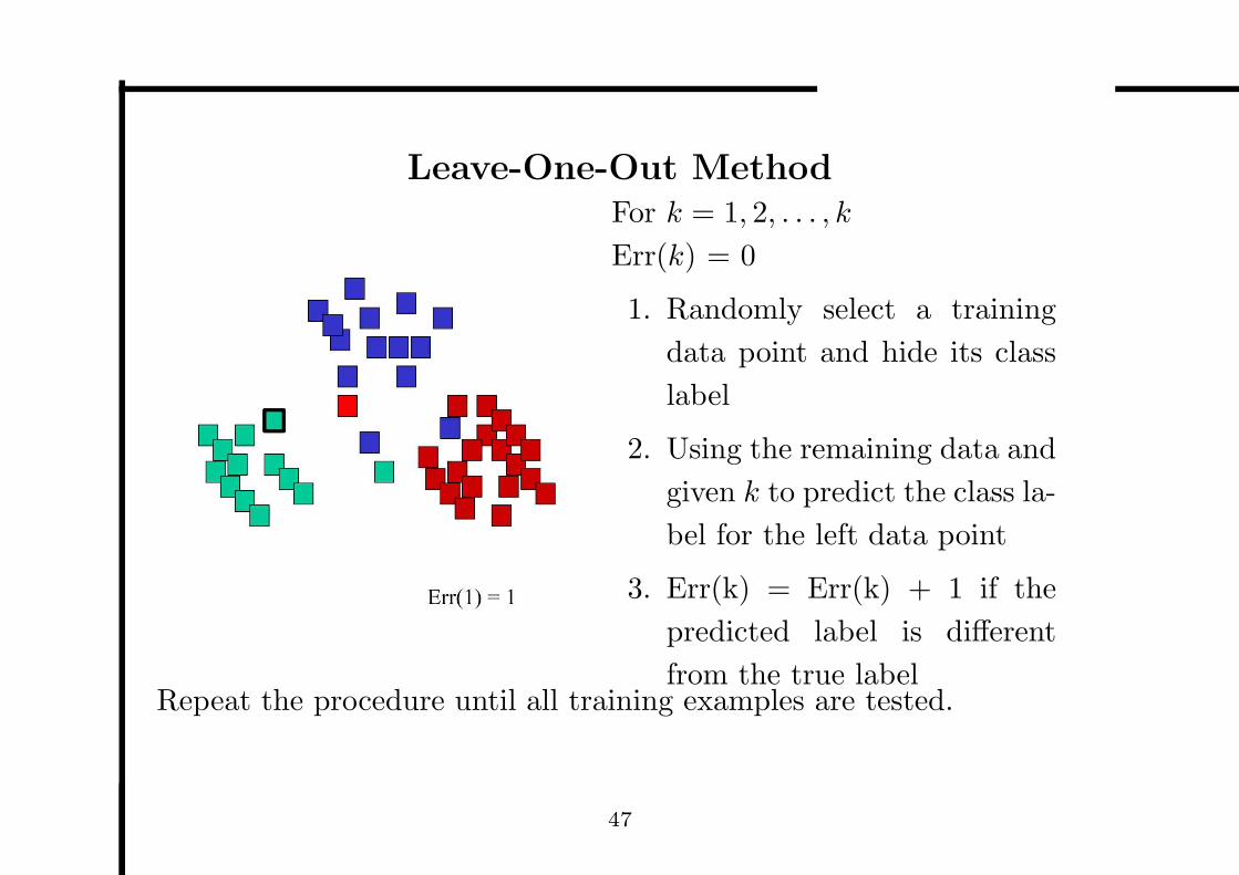
Leave-One-Out MethodFor k = 1, 2, . . . , k
Err(k) = 0
1. Randomly select a training
data point and hide its class
label
2. Using the remaining data and
given k to predict the class la-
bel for the left data point
3. Err(k) = Err(k) + 1 if the
predicted label is different
from the true labelRepeat the procedure until all training examples are tested.
Choose the k whose Err(k) is minimal
48
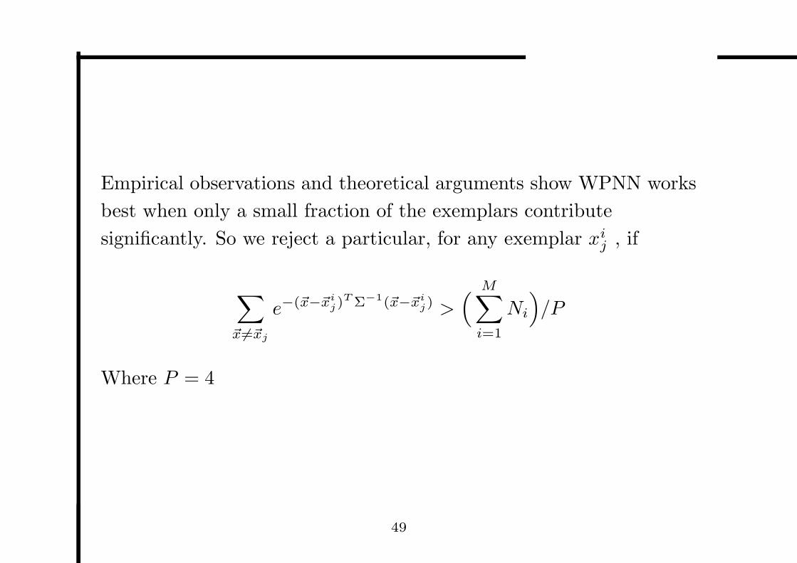
Empirical observations and theoretical arguments show WPNN works
best when only a small fraction of the exemplars contribute
significantly. So we reject a particular, for any exemplar xij , if
∑
~x6=~xj
e−(~x−~xij)
T Σ−1(~x−~xij) >
(
M∑
i=1
Ni
)
/P
Where P = 4
49
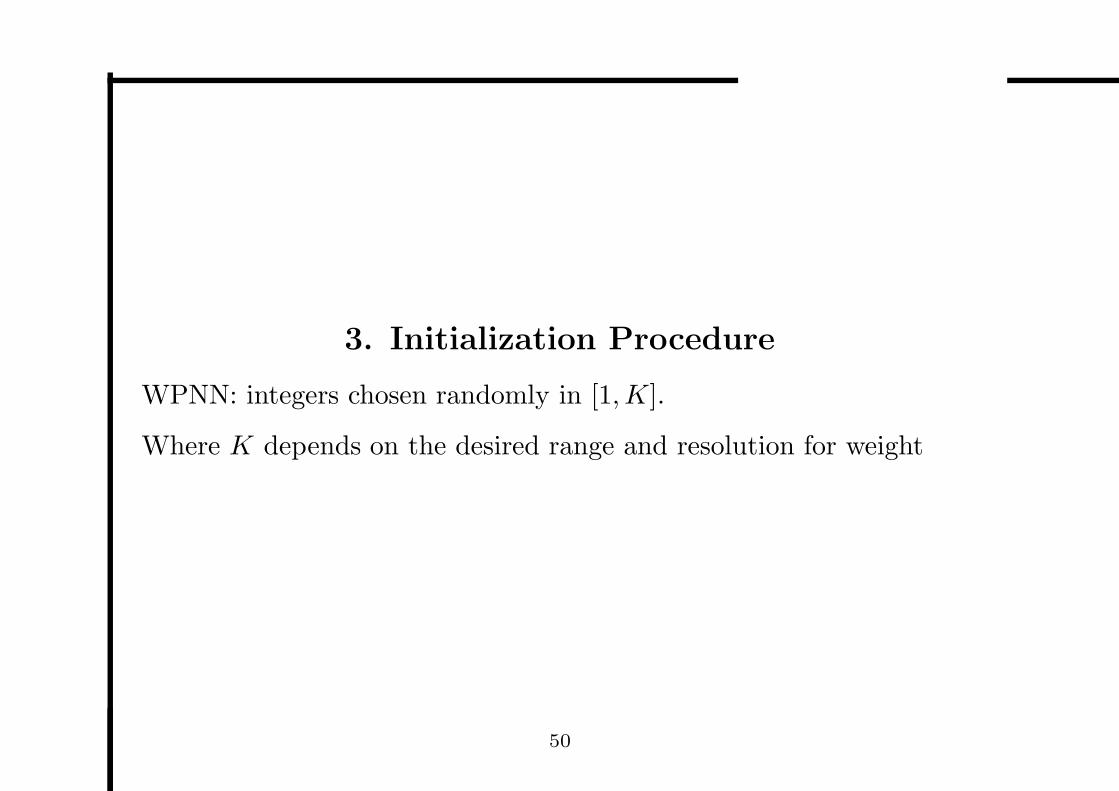
3. Initialization Procedure
WPNN: integers chosen randomly in [1, K].
Where K depends on the desired range and resolution for weight
50
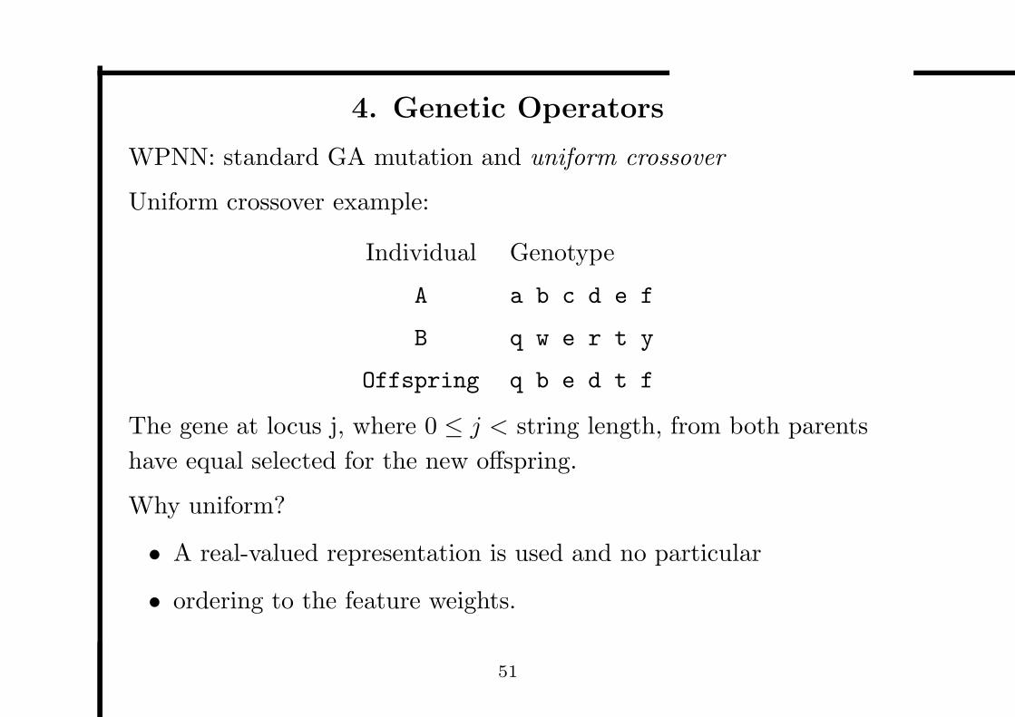
4. Genetic Operators
WPNN: standard GA mutation and uniform crossover
Uniform crossover example:
Individual Genotype
A a b c d e f
B q w e r t y
Offspring q b e d t f
The gene at locus j, where 0 ≤ j < string length, from both parents
have equal selected for the new offspring.
Why uniform?
• A real-valued representation is used and no particular
• ordering to the feature weights.
51
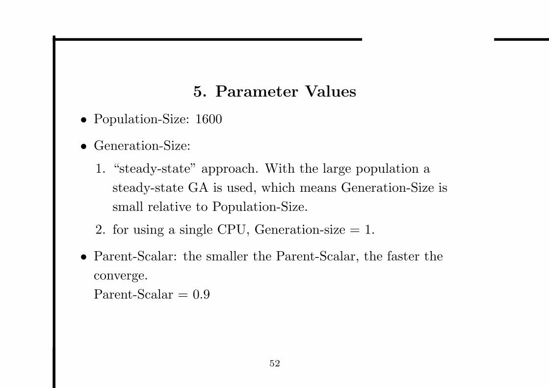
5. Parameter Values
• Population-Size: 1600
• Generation-Size:
1. “steady-state” approach. With the large population a
steady-state GA is used, which means Generation-Size is
small relative to Population-Size.
2. for using a single CPU, Generation-size = 1.
• Parent-Scalar: the smaller the Parent-Scalar, the faster the
converge.
Parent-Scalar = 0.9
52
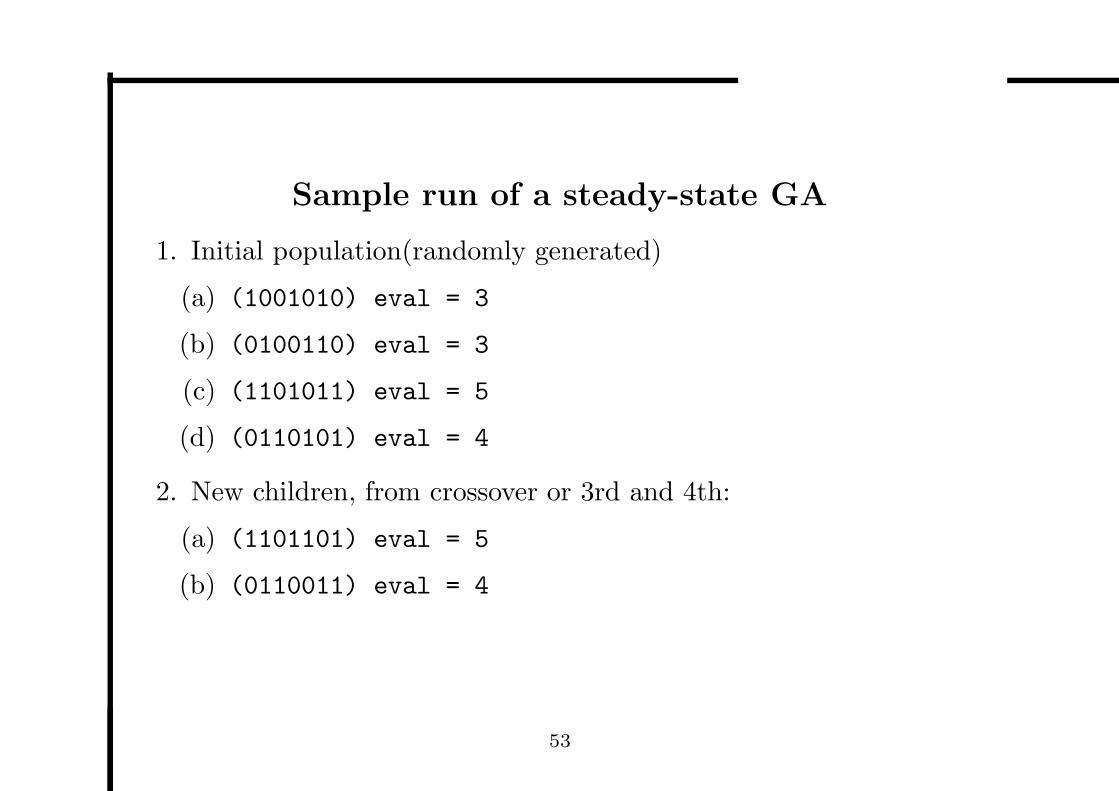
Sample run of a steady-state GA
1. Initial population(randomly generated)
(a) (1001010) eval = 3
(b) (0100110) eval = 3
(c) (1101011) eval = 5
(d) (0110101) eval = 4
2. New children, from crossover or 3rd and 4th:
(a) (1101101) eval = 5
(b) (0110011) eval = 4
53
Experimental Results — WPNN
WPNN was a new and untested algorithm, the experiments with
WPNN centered on the overall performance rather than on the
training algorithm.
54
Experimental Results — WPNN (Cont.)
4 data set designed are used to illustrate both the advantages and
shortcomings of WPNN.
55
Experimental Results — WPNN (Cont.)
First Data Set:
1. It is a training set that is generated during an effort to classify
simulated sonar signals.
2. 10 features
3. 5 classes
4. 516 total exemplars
56
Experimental Results — WPNN (Cont.)
Second Data Set: Same as first data set except:
5 more features are added (which were random numbers uniformly
distributed between 0 and 1 hence contained no information relevant
to classification)
57
Experimental Results — WPNN (Cont.)
Third Data Set: Same as first data set except:
10 irrelevent features are added. (total of 20 features)
58
Experimental Results — WPNN (Cont.)
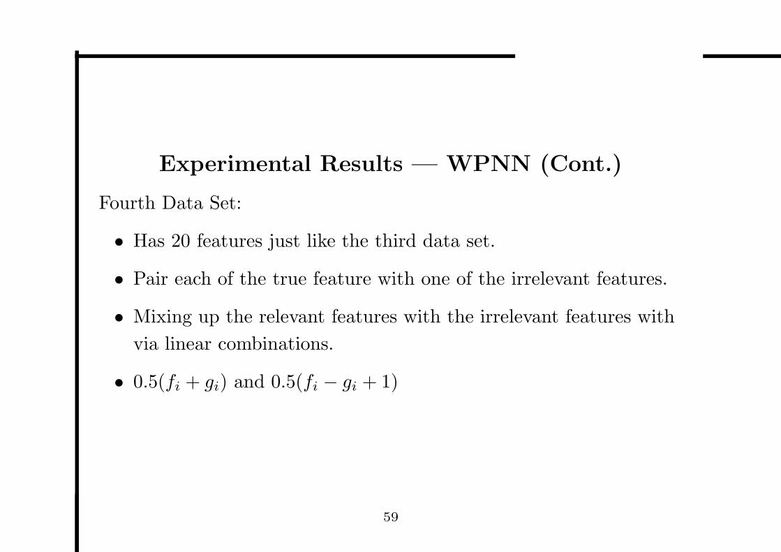
Fourth Data Set:
• Has 20 features just like the third data set.
• Pair each of the true feature with one of the irrelevant features.
• Mixing up the relevant features with the irrelevant features with
via linear combinations.
• 0.5(fi + gi) and 0.5(fi − gi + 1)
59
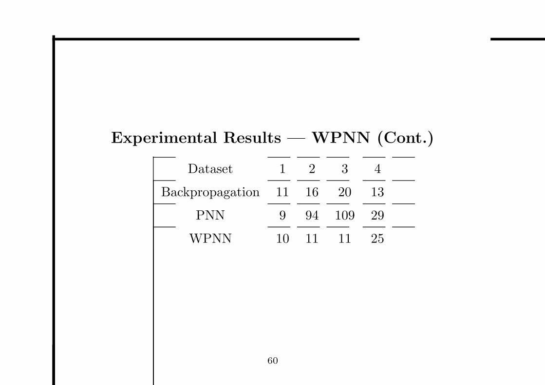
Experimental Results — WPNN (Cont.)
Dataset 1 2 3 4
Backpropagation 11 16 20 13
PNN 9 94 109 29
WPNN 10 11 11 25
60


![An integer programming approach to the OSPF weight setting ...sahmed/ospf.pdf · the weight setting problem. Ericsson et.al. [4] presented a genetic algorithm-based heuristic. Buriol](https://img.pdfslide.us/doc/110x75/5f2b6add5b776726c1258d19/an-integer-programming-approach-to-the-ospf-weight-setting-sahmedospfpdf.jpg)