Embed Size (px)
Citation preview

Neural Network Theory and Applications
2006
Willard L. Miranker Yale/DCS/TR-1376
December 2006


Table of Contents
Emergence of Language-Specific Phoneme Classifiers in Self-Organized Maps
Marek W. Doniec 1
Modeling Child Development using a Game Theoretic Approach and Genetic Algorithm
Laura J. Gehring 7
Cluster Analysis with Dynamically Restructuring Self-Organizing Maps
Daniel Holtmann-Rice 15
Dimensionality Reduction via Self-Organizing Feature Maps for Collaborative Filtering
Andrew R. Pariser 23
Face Recognition: A Comparative Study
Yan Sui 31
Note Onset Detection in Audio Sources
Andreas Voellmy 37

Emergence ofLanguage-Specific Phoneme Classifiers
in Self-Organized MapsMarek W. Doniec
Department of Computer ScienceYale University
New Haven, Connecticut 06511, [email protected]
Abstract— The difference between self-organizing maps basedphoneme classifiers that emerge for different input languagesis studied. For each such language a self-organizing map istrained on Mel-Frequency Cepstral Coefficient (MFCC) con-verted auditory input to form a phoneme classifier. Unsupervisedlearning is used as the training method. The emerging classesare then compared to the classes found in the InternationalPhonetic Alphabet. Particular class differences across languagesand speakers are discussed.
I. I NTRODUCTION AND RELATED WORK
Kepuska et al. [4] have shown that a hexagonal lattice self-organizing map (SOM) shows similar response patterns forthe same words and different response patterns for differentwords. They used 9 repetitions of 20 different words to trainand test their SOM. Kumpf et al. [7] showed that using aHidden Markov Model (HMM) they were able to classifyaccents within a group of Australian English speakers with anaccuracy of up to85.3%. Kangas [3] has shown that usinga time-dependant representation of Mel-Frequency CepstralCoefficients (MFCCs) can improve phoneme classificationfrom a 10.4% rate error to a5.0% rate error. However noneof these works have compared the resulting classes to theclasses found in the international phonetic alphabet (IPA). Thisalphabet is a much studied and widely accepted classificationof phonemes that provides a representation for phonemesof any spoken language [5]. A comparison of the classeslearned by a phoneme-recognition SOM to the IPA mightreveal strengths or weaknesses of training phoneme classifiersusing SOMs and possibly lead to improvement. Further apositive correspondence would suggest that SOMs are capableof capturing the functionality of the human auditory system.
We investigate the differences between phone classes ofdifferent languages. The languages are chosen to be differentenough so that a native speaker of one language usually hasa strong accent in the other language chosen. We first convertthe audio signal using Mel Frequency Cepstral Coefficients(MFCCs) which approximate the human auditory system’sresponse and are widely used in speech recognition systems[6], [8]. A self-organizing map is then trained on featurevectors for each of the languages tested. We use unsupervised
learning. The classes found in the resulting feature mapsare then compared to the IPA by submitting example wordsfor specific phonemes to the trained SOMs or by lookingat neurons that respond only to utterances from a particularlanguage. In particular we look for classes that are presentin at least one of the trained SOMs but not present theother trained SOMs. In addition we trained an SOM on twolanguages and examined at neurons that responded only toutterances from one of the two languages. We then identifiedthe phoneme class that these neurons correspond to. Finally weinvestigate the use of Principal Component Analysis (PCA) tofind phoneme classes and to compare phoneme classes fromdifferent languages.
The paper is organized as follows. Section II explains howdata was collected, preprocessed, and how the SOMs weretrained. Section III talks about differences between SOMsthat were trained on utterances from different speakers and indifferent languages. Section IV focuses on differences betweenlanguages. Section V examines the use of PCA to detectlanguage and speaker dependencies. Section VI summarizesthe results and Section VII contains brief critique.
II. M ETHODOLOGY
First we describe the setup for recording our wave samples.Then we describe how the self-organizing maps were trained,and we introduce a distance measure for the trained SOMs.
A. Recording
Wave files for the experiment were recorded at 8 bits monowith a 22 kHz sampling rate. A simple laptop microphonewas used and subjects were given a piece of text from anewspaper article or encyclopedia to read. We recorded twospeakers. The first speaker is a native English speaker and wasrecorded reading English texts. The second speaker is a nativeGerman speaker (the author of this paper) and was recordedreading German as well as English texts. For each language /speaker, three wave files were recorded for a total of 9 wavefiles. Each wave file has a 23 to 33 seconds duration andis about a paragraph of text long. In the following text theabbreviationS1E refers to the first speaker in English. The
Neural Network Theory and Applications 2006 - Yale/DCS/TR-1376 1
abbreviationsS2E and S2G stand for the second speaker inEnglish and German respectively.S2E,1 stands for the firstwave file recorded for the second speaker in English, etc.The index for wave files extends to the other abbreviationsappropriately.
For the second part of the paper in which we focus ondifferences across languages another set of data was collected.One native German speaker was recorded a total of 14 minutesreading 16 short text excerpts, 8 in English and 8 in German.The texts were divided into 4 groups, 2 English and 2 German,of which each is 3.5 minutes long. The groups are namedS1
E , S2E , S1
G, S2G. S1
E and S1G were used as the training sets,
S2E andS2
G were used as the test sets.
B. Training the Self-Organizing Maps
Recorded wave files were first processed using a simpleMatlab MFCC library obtained from the internet [9]. Thelibrary offers tools to convert the entire wave file into 20-dimensional MFCCs. The signal was converted using a Ham-ming window of size 32 msec and a hop time of 16 msec. Forexample, a 32 second wave file would result in 2000 MFCCsof size 20. This data was then presented a total of 20 times toa 10× 10 SOM.
C. A Distance Measure
To be able to compare the different SOMs we need adistance measure. For each SOMN and i ∈ {1, ..., 100} letN(i) ∈ R20 be the weight vector of theith neuron ofN .For j ∈ {1, ..., 20} let N(i, j) be the jth entry of the ith
weight vector ofN . An advantage of this notation is, that aSOM N can be represented by a100 × 20 matrix in whicheach row represents one neuron. Define the distance betweentwo neurons to be the square of the euclidian distance of theirweight vectors:
d′(N1(a), N2(b)) =20∑
k=1
(N1(a, k)−N2(b, k))2
Further define the bijective functionm : 1, ..., 20 →1, ..., 20 to be the optimal match between the neurons oftwo SOMs using the metric just define. This means thatmminimizes the following function:
d(N1, N2) =100∑
i=1
d′(N1(i), N2(m(i)))
Define this optimal match distance to be the distancebetween two SOMs. We see that this distance measure satisfiesthe three distance axioms:
1) d(N1, N2) ≥ 0 and d(N1, N2) = 0 iff N1 = N2.(Obvious.)
2) d(N1, N2) = d(N2, N1). (Obvious.)3) d(N1, N3) ≤ d(N1, N2) + d(N2, N3). If m12 is the
optimal match forN1, N2 andm23 is the optimal matchfor N2, N3 then the optimal match forN1, N3 is at leastas good asm23(m12).
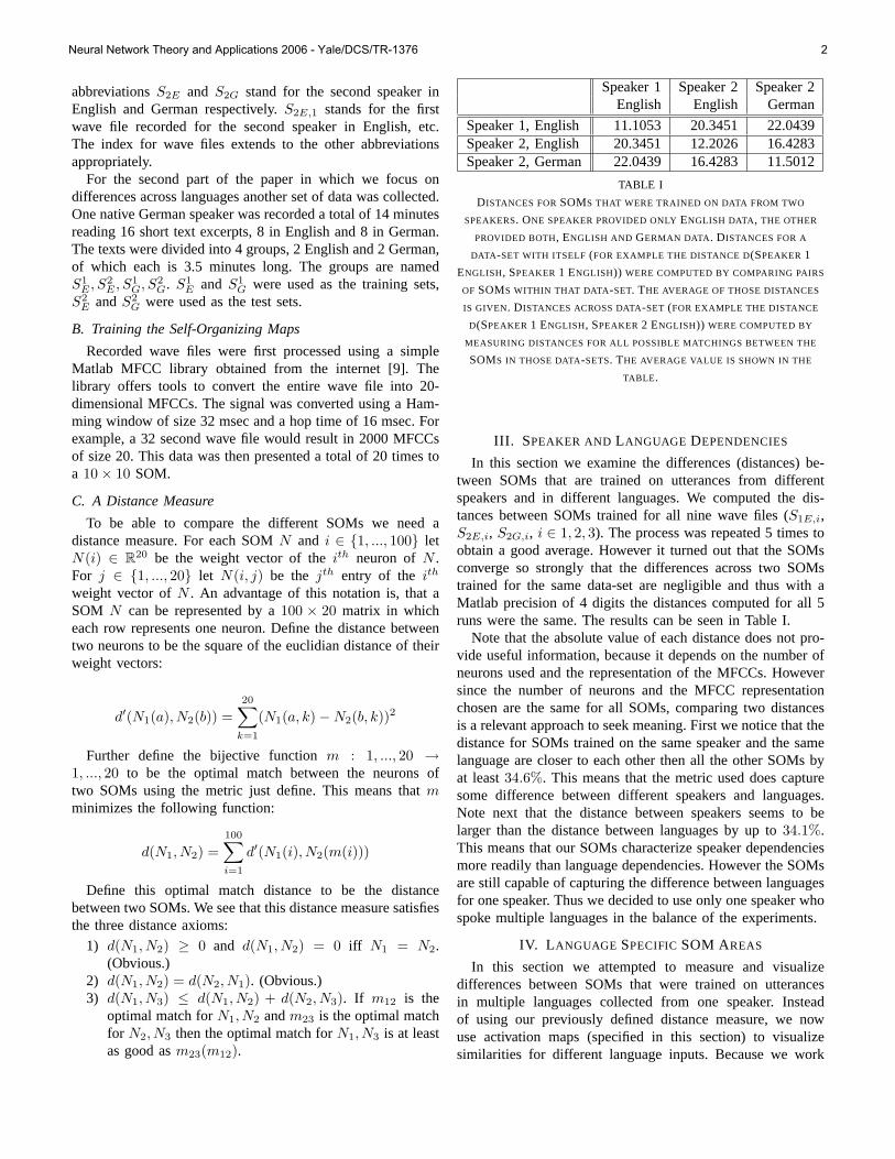
Speaker 1 Speaker 2 Speaker 2English English German
Speaker 1, English 11.1053 20.3451 22.0439Speaker 2, English 20.3451 12.2026 16.4283Speaker 2, German 22.0439 16.4283 11.5012
TABLE I
DISTANCES FORSOMS THAT WERE TRAINED ON DATA FROM TWO
SPEAKERS. ONE SPEAKER PROVIDED ONLYENGLISH DATA , THE OTHER
PROVIDED BOTH, ENGLISH AND GERMAN DATA . DISTANCES FOR A
DATA -SET WITH ITSELF (FOR EXAMPLE THE DISTANCE D(SPEAKER 1
ENGLISH, SPEAKER 1 ENGLISH)) WERE COMPUTED BY COMPARING PAIRS
OF SOMS WITHIN THAT DATA -SET. THE AVERAGE OF THOSE DISTANCES
IS GIVEN. DISTANCES ACROSS DATA-SET (FOR EXAMPLE THE DISTANCE
D(SPEAKER 1 ENGLISH, SPEAKER 2 ENGLISH)) WERE COMPUTED BY
MEASURING DISTANCES FOR ALL POSSIBLE MATCHINGS BETWEEN THE
SOMS IN THOSE DATA-SETS. THE AVERAGE VALUE IS SHOWN IN THE
TABLE .
III. SPEAKER AND LANGUAGE DEPENDENCIES
In this section we examine the differences (distances) be-tween SOMs that are trained on utterances from differentspeakers and in different languages. We computed the dis-tances between SOMs trained for all nine wave files (S1E,i,S2E,i, S2G,i, i ∈ 1, 2, 3). The process was repeated 5 times toobtain a good average. However it turned out that the SOMsconverge so strongly that the differences across two SOMstrained for the same data-set are negligible and thus with aMatlab precision of 4 digits the distances computed for all 5runs were the same. The results can be seen in Table I.
Note that the absolute value of each distance does not pro-vide useful information, because it depends on the number ofneurons used and the representation of the MFCCs. Howeversince the number of neurons and the MFCC representationchosen are the same for all SOMs, comparing two distancesis a relevant approach to seek meaning. First we notice that thedistance for SOMs trained on the same speaker and the samelanguage are closer to each other then all the other SOMs byat least34.6%. This means that the metric used does capturesome difference between different speakers and languages.Note next that the distance between speakers seems to belarger than the distance between languages by up to34.1%.This means that our SOMs characterize speaker dependenciesmore readily than language dependencies. However the SOMsare still capable of capturing the difference between languagesfor one speaker. Thus we decided to use only one speaker whospoke multiple languages in the balance of the experiments.
IV. L ANGUAGE SPECIFICSOM AREAS
In this section we attempted to measure and visualizedifferences between SOMs that were trained on utterancesin multiple languages collected from one speaker. Insteadof using our previously defined distance measure, we nowuse activation maps (specified in this section) to visualizesimilarities for different language inputs. Because we work
Neural Network Theory and Applications 2006 - Yale/DCS/TR-1376 2
with only one SOM, the distance measure does not enter intothis part of the study.
A. Training the SOM
Only the wave filesS1E and S1
G were used to train theSOM for this experiment. Recorded wave files were again firstprocessed using a simple Matlab MFCC library. To reduce theamount of data and keep training times reasonable, a Hammingwindow of size 100 msec and a hop time of 50 msec wasused. This data was then presented a total of 30 times to a10×10 SOM. Note that the rest of this section is based on theone particular SOM that resulted from such training. Howeverthis training process was repeated multiple times and whilethe resulting SOMs had a different spatial distribution of theneurons, they showed the same properties. These propertiesare presented in the following subsection.
B. Activation Maps
After training the SOM the four wave filesS1E , S2
E , S1G,
andS2G were processed into MFCCs. The newly trained SOM
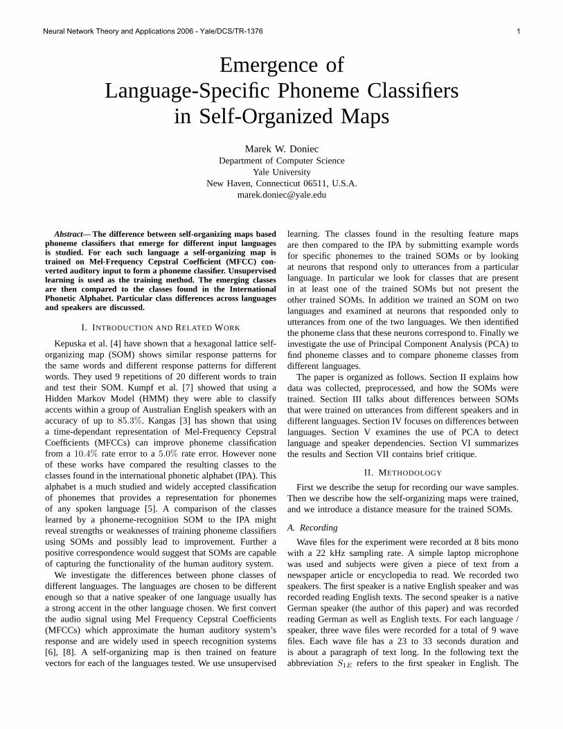
was used to classify the input vectors. For each input vectorthe Euclidean distance to all neurons was computed. Eachinput vector was then assigned the number of the neuronwith the smallest Euclidean distance to this input vector (Thatmeans this neuron fired for that particular input vector). Acount was kept how often each neuron would respond tothe input data stream. A separate counter was kept for eachof the four data streams resulting from the four wave files.The activation counts were then visualized in two activationmaps that are shown in Figure 1. In these maps a neuron’scolor intensity corresponds to the firing frequency for a givendata stream. The intensity of the color red is determined bythe firing frequency of that neuron during German utterance,the intensity of green corresponds to English. The color ofa neuron moves along the colorspectrum (from red to green)proportionately to the relative frequency of German to English.This means that a brightly red colored neuron respondedalmost only to German utterances whereas a green coloredneuron responded only to data streams of English utterances.Orange and Yellow colored neurons corresponded to a mixtureof utterances in both languages. The first activation map(Figure 1(a)) represents the SOMs response to data createdfrom the training set wave filesS1
E and S1G. The second
activation map (Figure 1(b)) represents the SOM’s responseto data created from the test set wave filesS2
E andS2G.
C. Observations
Note that the SOM develops the following four types ofneurons:
1) There are a few neurons that do not respond to utterancesfrom either language. For example, neuron(10, 3) isalmost entirely dark in both activation maps (For neuronnumbering, see the caption of Figure 1). These neuronsare most likely a result of the neighborhood-rule, i.e. twoneighboring neurons that are far apart ’pull’ this neuroninto a space that is not used by the input.
2) Most neurons respond in similar ways to utterances inboth languages. This is to be expected. Examples areneurons(1, 1) and (1, 10).
3) Some neurons respond almost exclusively to utter-ances in German. These neurons represent sounds andphonemes that occur predominantly in German. Onesuch neuron is neuron(1, 9).
4) Some neurons respond almost exclusively to utter-ances in English. These neurons represent sounds andphonemes that occur predominantly in English. Onesuch neuron is neuron(5, 7).
The occurrence of neurons that respond only to utterancesin one langauge is a sign that the SOM does develop language-specific regions. To show that these regions are not entirelytraining-set dependant we produced a second activation mapusing utterances from a separate test set. As can be ex-pected the activation maps are not identical, however thepredominance of certain similarities supports the hypothesisthat SOMs develop language specific neurons. In the exampleillustrated in Figure 1 we can see that for both activationmaps the lower right corner is German-dominated and that thecenter of the SOM is English-dominated. The left top cornerresponds frequently for both languages. As we shall see laterit corresponds to silence (i.e., a pause) between words.
D. A Closer Look at Single Neurons
To illustrate the occurrence of each of the four neuronalclasses discussed above and to show that language dependantneurons emerged during training, we have singled out theparts of the wave files that activate certain neurons that arepredominant in one or in both languages, as the case maybe. We give the total response time of neurons to utterancesin different languages. The total response time for a neuronis calculated by multiplying the number of input vectors towhich this neuron responded by the stepping size that wasused to calculate the input vectors (50 msec).
First we examined the brightly yellow colored neuronnumber(1, 1). We found that this neuron responded to MFCCsthat represented silence. For the training set this neuronresponded for a total of 7.6 sec for German and 5.75 secfor English. For the test set the total response time was 12.3sec for German and 7.75 sec for English. This suggests thatwhen speaking German, our speaker paused longer betweenwords. However pauses might also have been classified byneighboring neurons. Since pauses occur frequently betweenwords in both languages, this neuron(1, 1) is colored a brightyellow in the activation maps.
For further analysis we examined a neuron that exhibiteda strong response only for MFCCs created from Englishutterances. Neuron(5, 7) is colored green and responded atotal of 0.05 sec for German and 3.15 sec for English inthe training set and 0.05 sec for German and 3.15 sec forEnglish in the test set. Here is a list of some of the wordsduring which neuron(5, 7) fired. Each word is accompaniedby a pronunciation transcription as presented by the Merriam-Webster Online Dictionary [10].
Neural Network Theory and Applications 2006 - Yale/DCS/TR-1376 3

(a) SOM activation map for German and English utterances fromthe training set.
(b) SOM activation map for German and English utterances fromthe test set.
Fig. 1. These SOM activation maps display the response frequency of neurons to utterances in English (green) and German (red). Yellow denotes a neuronthat responded frequently during utterances from both languages. The activation map on the left shows neuron firing frequencies during utterances from thesame sample set that was used to train the SOM. The right activation map shows neuron firing frequencies during utterances from a separate test set. Thesimilarities of the images show that certain neurons respond more frequently during utterances in English than utterances in German and other neurons respondmore frequently during utterances in German. The neurons are numbered lexicographically in row/column order. The bright yellow neuron at the top in eachactivation map is thus numbered(1, 1).
• thirty [’th&r-tE ]• traverse [tr&-’v&rs ]• effort [’e-f&rt ]• computer [k&m-’py\ u-t&r”]• service [’s&r-v&s ]• aircraft [’er-\ kraft”]The neuron responded in particular to the [&r], which is
pronounced like the ur/er in further.Neuron(1, 9) was also examined. It is colored a dark red
and responded for a total of 4.7 sec for German and 0.45 secfor English for the training set and 4.65 sec for German and1.0 sec for English for the test set. This neuron correspondedto the nasal [n] sound as in ’nice’ which occurs less frequentlyin English then it does in German.
Similarly to neuron(1, 9), neuron(10, 4) responded morefrequently to German than to English. It represented the [sh]sound as in ’shoe’. It responded for a total of 4.0 sec forGerman and 2.05 sec for English for the training set and 4.5sec for German and 2.9 sec for English for the test set.
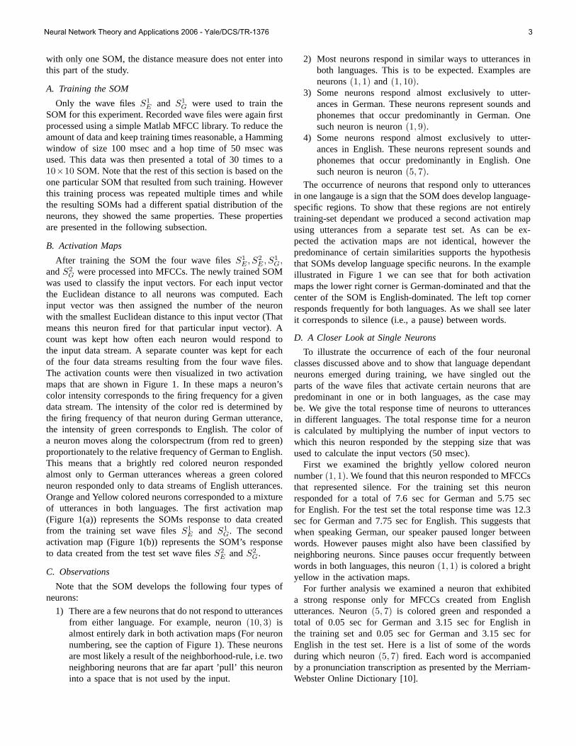
We also examined the [th] phoneme that does not occurin the German language but frequently occurs in English inwords like ’this’ and ’that’. A small test file that containedonly that words ’this’ and ’that’ was recorded and the resultingMFCCs were classified with our bilingual SOM. The result isshown in figure 2. This image helped us identify the neuronthat corresponded to [th]. This was neuron(6, 6) for thisparticular SOM. Neuron(6, 6) responded for a total of 0.8sec for German and 2.35 seconds for English for the trainingset and 1.45 sec for German and 3.6 sec for English for the
Fig. 2. Activation map for our bilingual SOM in reaction to a recording of’this’ and ’that’ utterances. Dark blue means no activation, light blue corre-sponds to medium activation, yellow and red correspond to high activation.
test set. While it responded far more frequently to Englishthen to German it is still surprising that this neuron respondedto German at all, since the [th] sound does not occur in theGerman language. We see two possible reasons for this:
1) The most likely reason is that the speaker recorded was anative German speaker whose pronunciation very likely
Neural Network Theory and Applications 2006 - Yale/DCS/TR-1376 4

Speaker 1 Speaker 2 Speaker 2English English German
Speaker 1, English 0.2852 0.7209 0.8076Speaker 2, English 0.7209 0.2146 0.3766Speaker 2, German 0.8076 0.3766 0.2536
TABLE II
AVERAGE DISTANCES BETWEEN THE FIRST PRINCIPAL COMPONENTS FOR
OUR WAVE FILES SORTED BY GROUP(LANGUAGE, SPEAKER). THE
ABSOLUTE VALUES ARE OF NO MEANING, HOWEVER THERE IS A
SIGNIFICANT DIFFERENCE BETWEEN THE DISTANCE FOR SPEAKERS AND
THE DISTANCE FOR LANGUAGES. THIS SUGGESTS THATPCA IS ABLE TO
CAPTURE SPEAKER DIFFERENCES.
biased the result.2) The resolution of the SOM might cause two sounds to
be classified by one neuron. Thus the same neuron mightrespond to similar sounds like [v].
V. PRINCIPAL COMPONENTANALYSIS
We also investigated the use of Principal Component Anal-ysis (PCA) to recognize speaker or language dependencies.PCA is a good candidate because it both extracts the mostsignificant components and allows for a dimensionality reduc-tion of the data. We hoped that we could identify componentsthat would help identify the speaker or the language.
The input wave files were again transformed into MFCCsusing 100 msec Hamming windows and a hop time of 50msec. We use the files (S1E,i, S2E,i, S2G,i, i ∈ 1, 2, 3). Wethen applied PCA to each data stream and saved the principalcomponents (20 components for each file, each componentof size 20). For each principal component and each pair offiles we computed the Euclidian distance giving a total of9 × 9 = 81 distances. The distances were then averagedover comparisons between files from the same group (thereare three groups:S1E , S2E , and S2G). This resulted in 20tables, one for each principal component. Each table givesthe average distances for this particular principal componentbetween languages and speakers. We found that the firstcomponent represented the distances between speakers wellas can be seen in Table II. However none of the componentsseemed to represent differences in language.
In a second analysis we used PCA to reduce the inputspace for our SOM training algorithm. For this the MFCCtransformed filesS1
E , S2E , S1
G, andS2G were concatenated and
PCA was applied to the resulting data stream. This time therepresentation in principal components was input to the SOMas input. The results were similar as in the that in Section IV.
However we found the following problem in utilizingPCA together with SOMs. PCA generates different principalcomponents for different input files as shown in Table II.This results in the problem that if we transform two filesseparately then their representation in their respective principalcomponents are of no value to the SOM, because they areindependent of each other. We tried to represent additional
data in the principal component space of the training data butonly with marginal results.
VI. SUMMARY OF RESULTS
We showed that training SOMs on MFCCs results in SOMsthat are both, speaker and language dependant. This resultwas obtained by comparing the SOMs with a specified metric.This suggests that SOMs can be used to differentiate betweenlanguages and between speakers.
We further showed that SOMs do capture differences be-tween languages that can be easily made discernable. Inparticular we showed that if an SOM is trained with twolanguages then some neurons represent sounds that are uniqueor predominant in one of the languages. An additional resultwas that independently of the language used, the SOM hascertain neurons that correspond to silence (a pause) and areactivated more frequently than other neurons in the sameSOM.
We showed that PCA might be able to extract speakerdifferences but most likely is not suitable to extract languagedifferences. Further we explained that it is not possible to usePCA to preprocess the input to the SOM training algorithmbecause PCA will generate different principal components fortwo separate input samples. Thus representing each samplein the principal component space does not allow for a goodcomparison of two different samples.
VII. D ISCUSSION
The results suggest that training an SOM on unlabeledspeech data can result in the formation of a phoneme classifierin which groups of neurons or single neurons correspond todifferent phonemes. Although these phonemes are not labeledthey seem to represent the phoneme space of spoken languageswell. These SOMs help to further reduce the dimensionalityof the input and could be of use for further classification andspeech recognition tasks. The advantage over existing work isthat our system uses unsupervised learning and thus needs nofeedback.
We have found that the SOMs capture speaker as well aslanguage differences. This suggests that an SOM might beused to discern certain simple classes of speakers. An analogof this is the preferential response of infants to their mother’svoice as found by Mehler et al. [12].
The language differences captured suggest that an SOMadapts to a certain language and its phonemes. This is alsosimilar to findings in infants who habituate themselves to aparticular set of phonemes and tend to attenuate non-nativephonemes during advanced langauge learning [11]. Furtherwe have shown that if trained with two languages at oncean SOM can learn both phoneme sets and even distinguishbetween sounds that occur only in one of the languages. Forfuture work we envision a system that learns to differentiatebetween several different languages based on the firing patternof a trained SOM.
Another utilization of such an SOM could be speech seg-mentation. We observed that the neurons representing silence
Neural Network Theory and Applications 2006 - Yale/DCS/TR-1376 5
in the SOM fire more frequently then any other neuron(see Figure 1). This suggests that if indeed silence is thepredominant feature vector, our system has developed a setof neurons that represent word-boundary signals. So not onlydoes our SOM learn to classify phonemes but it could providea subsequent speech recognition system with word boundaryinformation.
We showed that PCA is not well suited for preprocessing theinput for the SOM in the case of building phoneme classifiers.We believe however that PCA might serve to extract principalcomponents from a large data set for in the identification ofspeakers. The reason that PCA demonstrated no utility forpreprocessing is that different input files produced differentprincipal components. This happens especially if the input filesare small and thus provide only a small sample of training data.Further study will show whether the principal components willtend to stabilize for large bodies of data (multiple hours ofrecordings for each speaker / language combination). If suchfixed points exist they might prove useful for preprocessingthe speech signal.
Future work should include a more detailed analysis ofthe exhibited behaviors. The results obtained in this studyare based on noisy data that was collected under suboptimalconditions from only two subjects. We believe that a largescale study employing data from many subjects might revealadditional features and allow testing of the interaction betweendifferent languages and speakers. The reason that we usedonly one speaker for the second part of the study is thatcurrently there is no good method for extracting speakerindependent feature vectors from speech. MFCC still capturesthe base frequency and possibly other speaker dependentfeatures and thus does not allow for efficient comparison oflanguages across speakers. Current work on speaker inde-pendent phoneme classification usually trains classifiers on alarge body of subjects [13]. While these classifiers learn togeneralize across different subjects, they are still presentedwith speaker-dependent input such as MFCCs. A similarapproach might be used in combination with the methodspresented here. Naturally this would require a large body ofdata.
We have shown that the unsupervised learning of SOMswith as few as 100 neurons enables extraction of speakerand langauge differences. We showed that some can extractadditional useful information such as word boundaries. ThusSOMs are well suited for use in unsupervised learning systemsfor word grounding (learning the meaning of words) andlanguage recognition. We have also shown that SOM phonemerecognizers show learning and recognition behavior similar tothat of human infants.
REFERENCES
[1] C. Yu, D. H. Ballard and R. N. Aslin,The Role of Embodied Intentionin Early Lexical Acquisition, Coginitive Science, 29(6), 961-1005, 2005.
[2] D. K. Roy and A. P. PentlandLearning words from sights and sounds:a computational model, Cognitive Science, 26(1), 113-146, 2001.
[3] J. Kangas,Phoneme recognition using time-dependent versions of self-organizing maps, In Proceedings of the International Conference onAcoustics, Speech and Signal Processing, p. 101-104, Toronto, Canada,May 1991.
[4] V. Z. Kepuska and J. N. Gowdy,Investigation of phonemic context inspeech using self-organizing feature maps, IEEE International Conferenceon Acoustics, Speech and Signal Processing, ICASSP ’89, Glasgow,Scotland, May 1989.
[5] International Phonetic Association,Handbook of the International Pho-netic Association - A Guide to the Use of the International PhoneticAlphabet, July 1999.
[6] Z. Fang, Z. Guoliang and S. Zhanjiang,Comparison of different im-plementations of MFCC, Journal of Computer Science and Technology,16(6), 582-589, 2001.
[7] K. Kumpf and R. W. King,Automatic accent classification of foreignaccented australian english speech, In Proceedings of 4th InternationalConference on Spoken Language Processing, Philadelphia, USA, October1996.
[8] Mel frequency cepstral coefficient, Wikipedia,http://en.wikipedia.org/wiki/Melfrequencycepstralcoefficient, 2006.
[9] PLP and RASTA (and MFCC, and inversion) in Matlab, D. Ellis,http://labrosa.ee.columbia.edu/matlab/rastamat/, 2006.
[10] Merriam-Webster’s Online Dictionary, www.m-w.com, 2006.[11] D. Burnham,Language specificity in the development of auditory-visual
speech perception, R. Campbell & B. Dodd (Eds.), Hearing bye eyeII: Adances in psychology of speechreading and auditory-visual speech.Hove, england: erlbaum UK, pp. 27-60, 1998.
[12] J. Mehler, J. Bertonicini, M. Barriere,Infant recognition of mother’svoice, Journal of Perception, 7(5):491-7, 1978.
[13] M. Antal, Speaker Independent Phoneme Classification in ContinuousSpeech, Studia Univ. Babes-Bolyai Informatica, Vol. XLIX, No. 2, pp.55-64, 2004.
Neural Network Theory and Applications 2006 - Yale/DCS/TR-1376 6

Abstract— A child’s development of mind is studied using
iterations of a Prisoner’s Dilemma game in conjunction with a genetic algorithm. Situations where a poor parent is replaced mid-set with a near optimal parent are investigated. This provides a model for the situation where a child in the care of an individual suffering from a form of psychopathy such as depression are witness to their recovery or removed to more attentive care. A genetic algorithm is used to represent the child’s memory throughout parental development. As hypothesized the model demonstrates rates of change in fitness and mental development which correlate to the length and quality of care received by the child in each distinct section of the trial.
Index Terms—Parental Psychopathology, Theory of Mind, Game Theory
I. INTRODUCTION
S adults, the vast majority of humans realize that there is not one collective mind in use by the entire population.
Beliefs and the substance of knowledge vary from person to person. Such an awareness of the individuality of others does not seem to be inherent from birth, but develops as a child does with common tests for this ability usually being successfully completed by children who are, at the very youngest, 3 to 4 years old[2]. Understanding how such ability arises remains a topic of continued psychological research. Studies have shown that one factor affecting the time before emergence of a full theory of mind is the amount and type of discourse a child is exposed to[4]. Interactions between parents and children can be grouped into two broad categories, “mentalizing” and “non-mentalizing”[5]. Mentalizing responses to a child would include any in which a caregiver recognizes and draws attention to the child’s state of mind, and how it relates to their actions and reactions to events. Non-mentalizing responses deal more directly with actions, events, and consequences with no reference to how a child’s mental state was involved. The ratio of mentalizing to non-mentalizing interactions children and caregivers engage in would necessarily vary due to environmental factors. However, not all children are given the opportunity to interact with a “normal” adult. We will develop a model for the interaction of a normal
Manuscript received November 28, 2006. L. J. Gehring , junior at Yale Universtiy( e-mail: [email protected]).
child with a normal parent and contrast this with relations formed by a child with some imperfect parent. Such a model could be equated with situations in which a child is interacting with a caregiver suffering some form of psychopathology, such as depression, which affects ability to interact in a manner comparable to that accomplished by normal adults. Interactions with such “semi-developed” adults should delay child’s development[1]. Further, we will model the effects of switching from a semi-developed parent to a fully-developed one such as would occur in a real-life situation when a parent seeks help for their condition or when children are moved to a more stable environment. Such a situation should influence the child’s rate of development. An initial drop in development could be expected directly after such a shift followed by an increased rate of development correlating with the increased efficacy of the current caregiver over the previous. A game theoretic methodology such as the one outlined by Mayes and Miranker[5] will be used to model this interaction and the resulting development of the child. Here a version of the Prisoner’s Dilemma was suggested to model the interaction between caregiver and child while the development of mind would be represented by the convergence of a child’s strategy of play to one beneficial in the current context. The child’s memory of past exchanges is represented with a genetic algorithm and is used to help choose the child’s course of action
II. THE MODEL
A. Initializing Prisoner’s Dilemma
In the interest of clarity, female pronouns will be used to refer to the parent while male pronouns will be used in reference to the child from this point on. In the model, the parent and child each have two options. She has the option of ignoring the child which requires an absolute minimal effort, or paying attention to him which does require effort. The child’s two options are to use his intuition which is associated with a minimal cost, or to use his mind, which would use more energy. Both parties have the goal of expending as little effort while reaping the benefits of the other’s efforts. The ideal situation, from a parent’s perspective, therefore, would be one in which the child is constantly ignored and yet continues to use his mind. Using the mind causes him to mature. The child’s decision to use mind would therefore benefit the parent
Modeling Child Development using a Game Theoretic Approach and Genetic Algorithm
Laura J. Gehring
A
Neural Network Theory and Applications 2006 - Yale/DCS/TR-1376 7
by reducing the period of time in which he was dependent on her parents. The child’s ideal situation, in contrast, would be to continuously choose to use intuition and receive attention from the parent. In such a case, the child is not neglected and does not have to pay for the attentions received with the cost of using his mind instead of intuition. Remaining possible scenarios are that both parties choose actions requiring effort or that both parties choose actions requiring minimal effort. These two courses result in changes which are equal in both the parent and child. These relative costs can be assimilated into the payoff matrix of Table I.
Table I: Child\Parent Action Payoffs
Child\ Adult Attend Ignore Mind R, R S, T Intuition T, S P, P
When values of T>R>P>S are implemented a true Prisoner’s dilemma is created which models the previously defined interactions as desired. The value each participant in the game receives hinges on the actions of their opponent. In this case, the best results for an individual are the product of successfully tricking the other player into doing more work while engaging in less itself. The opponent then receives the lowest possible return value. In the real world, such actions result in a loss of trust. A rational agent would learn from such an experience and when confronted with that same type of situation would be more apt to anticipate another deception. The logical course would be to minimize losses by engaging in the less expensive activity. This kind of activity would naturally degrade into the (P,P) situation. Cooperating to achieve the (R,R) situation would benefit both parties more in the long term, but is much more difficult to achieve because of the increased risk associated with that position.
B. Memory
Each iteration of the Prisoner’s Dilemma will result in a move by the child and a reaction from the parent. To isolate the reactions of the child, it will be assumed for this model that the parent’s strategy will not be affected by game play and only alters at the designated time when it is shifted to its more/less optimal counterpart. For ease of implementation and because of its proven efficacy, an optimal parent will use the tit-for-tat strategy and respond to the child’s action with an action of corresponding cost. For example, if the child chooses Mind she will counter with Attend while if he opts for Intuition she will choose Ignore.
When a child begins, it has no memory and is obliged to make a random play. At the end of the iteration, it receives the payoff determined by the above matrix. This amount is added to the child’s fitness level, which is initially set to 0. This fitness level provides an indication of how well he understands his adversary. A high fitness value results from typically high values returned after participating in the Prisoner’s Dilemma and indicates a better understanding of the strategy being used by the opponent and its successful exploitation. At this point a
decision, on the basis of payoff and a random variable, is made to either include the play sequence in memory or to discard it.
A child’s memory is represented by a tree. Each node represents a point of play and has two branches which represent the two possible actions that the child may take at that instant. Additionally, a weight, initially set to zero, is associated with each of these options. These two branches lead to two more nodes each with two more branches and so on. The weight associated with each branch signifies how successful a given choice at this node has been at increasing the child’s fitness in the past. All weights are initially set to 0, meaning that there is neither benefit nor loss associated with each choice at that point. However, as the child ages and creates memories, these weights come to reflect the outcomes of previous decisions. When an event is committed to memory the outcome is associated not only with the most recent action, but also with the sequence of deeds leading up to the most recent choice. Weights corresponding with the action chosen must be updated in each of the specific nodes reached by following the increasingly complex sequence of previously chosen actions up to the depth of the child’s ability to recall specific past choices. For example, if he could only remember the last four choices made, it would be necessary to change the weights of those nodes reached by walking the last 4, 3, 2, and 1 actions chosen by the child.
If a child chooses to use its memory, a number of past sequences equal to the child’s memory recall level are summoned from the end of the record of past child choices. Using these, the most beneficial sequence may be selected using a genetic algorithm, and a choice between the two current options is returned. Weights of the associated sequence of plays and the child’s fitness are altered based on payoff garnered as a result of the choice.
C. Introduction of Psychopathy
Each run of the simulation will consist of time spent with an optimal parent and time with a suboptimal parent. The optimal parent will use a pure tit-for-tat strategy while the suboptimal parent will follow a similar strategy, but interspersed with noise created by random deviations from that strategy. The amount of deviation will be controlled between trials to investigate effects of more and less deviation from the tit-for-tat strategy. The actions of the suboptimal parent will be determined by the value of a randomly generated variable, which when greater than some threshold will choose to play randomly rather than use tit-for-tat. This threshold may be increased (to increase optimality) or decreased (to increase the number of random plays).
The model will consist of having the child play the suboptimal parent for a number of iterations before switching to the optimal parent and measuring how long it takes the child to reach a strategy for use with the fitter parent which provides the highest payoffs as they have been previously defined. Each segment of the experiment will consist of 50 distinct games so that an average course of development less skewed by chance may be obtained. Each game will be composed of 100 iterations of the Prisoner’s Dilemma, or 200 combined moves made by the child and parent. Each game will begin with a fresh child with no previous memories and no record of
Neural Network Theory and Applications 2006 - Yale/DCS/TR-1376 8

past moves. The goal will be to determine and compare the effects of exposure to suboptimal parents of varying degrees of degradation on the child’s development and ability to recover when later exposed to optimal parenting.
III. EXPERIMENT
A. Overview
Initially, the model was run solely with the optimal parent and subsequently completed runs with each of the suboptimal parents to be investigated to create points of comparison. Next, the game was executed several times with differing levels of degradation in the initial suboptimal parent before switching to the optimal caregiver after 50 iterations involving the suboptimal player. After that, the length of exposure to the suboptimal parent was modified to evaluate the effects of varying amounts of exposure to the same suboptimal caregiver. Finally, the effects of exposing a child to a more effective, though still suboptimal, parent following 50 iterations with a suboptimal parent will be explored. During each of these trials, records will be kept regarding the child’s fitness which correlates with the values received from engaging in the Prisoner’s Dilemma. Also, Maturity of the mind will be recorded. Maturity may be defined as the number of times he has chosen mind over intuition. As the child plays, strategies should form, which when followed, cause the child’s fitness to grow more quickly than when playing randomly. Since a tit-for-tat strategy is being used, the response strategy for the child is to always choose mind. Playing intuition against a parent utilizing a strict tit-for-tat strategy will always yield a lower payoff than that achieved by playing mind. The emergence of this strategy will also be monitored during each of these trials and recorded. Point of emergence will be defined as the point at which child chooses to play mind over intuition during ten consecutive iterations. As the optimality of the parent decreases and the number random plays made by the parent increases, the value of constantly choosing mind degrades and children are slower to adopt it because of its decreased utility. In fact, those children paired with a parent who makes only random plays will soon adopt the opposite strategy of always choosing intuition so as to minimize losses against this irrational agent.
B. Optimal Exposure
Under optimal conditions, the parent counters all moves of the child using a pure tit-for-tat strategy. Results for these trials are displayed in Tables II.a-c. Here the strategy arrives very early on averaging at around 4.68 iterations into the trial with a standard deviation of 3.71. The average maturity, or number of times the mind was chosen, at the end of the trial was 97.54 with a standard deviation of 1.25 while fitness at the end of the runs averaged 95.08 with a standard deviation of 2.50.
C. Varied Suboptimal Exposures
To contrast with the optimal parent, trials of 100 iterations were also performed with parents of varying levels of random play. Information from these trials is summarized in Tables
II.a-c alongside information from the optimal trial as a point of comparison.
Table II.a: Emergence of strategy
Parent Exposure
Mean Number Plays to Emergence
Stand. Dev.
Non-maturing
Optimal 4.68 3.71 0
70% Optimal 10.2 8.25 0
50% Optimal 22.26 20.88 0
30% Optimal 66.08* 20.25* 21 (42%)
Random Play --------- ---------- 49 (98%)
*To make the mean and standard deviation of trials where many runs did not converge more meaningful, a value of 100 was substituted as the point of maturation for such runs. This helps offset the somewhat lesser values for each of these that would otherwise occur.
Table II.b: Maturity
Parent Exposure
Mean End Maturity
Stand. Dev.
Optimal 97.54 1.25
70% Optimal 95.04 3.61
50% Optimal 88.22 10.33
30% Optimal 55.34 29.77
Random Play 7.9 6.34
Table II.c: Fitness
Parent Exposure
Mean End Fitness
Stand. Dev.
Optimal 95.08 2.50
70% Optimal 46.7 12.62
50% Optimal 21.06 14.85
30% Optimal 1.98 14.23
Random Play 36.88 20.24
It is important to note, that when a completely random parent
is used with no adherence to a tit-for-tat strategy that the child does in fact reach an effective strategy of sorts, it simply never uses its mind and maturity, as it is measured, suffers. With random plays this would equate to an overall increase in fitness when the values of the payoff are arranged symmetrically and the parent gives attention and ignores equally. However, this strategy is relatively useless against a parent with a strategy like tit-for-tat where the child will never receive a reward, or positive payoff, for not using his mind. As the amount of random activity is increased the fitness of the child initially decreases as it makes the transition between two very different strategies which is why the fitness is so low when the parent is only playing at a 30% optimal level. Further decreases in random play firmly establish an effective
Neural Network Theory and Applications 2006 - Yale/DCS/TR-1376 9

strategy to be used in conjunction with tit-for-tat. Graph III in the appendix illustrates these two clear strategies adopted by the child and the ways in which fitness and maturity are affected.
It is also appropriate that the standard deviation for aspects of measurement like fitness and maturity tend to increase as random play is increased. The exceptions to this rule tend to occur at points of key change such as the instance where there are an unusual number of trials which never converged to the strategy and thus affected the mean emergence and standard deviation.
D. Varied Suboptimal Parenting followed by Optimal Parenting
The ability of a child to converge upon the ideal tit-for-tat response strategy following exposure to varied levels of suboptimal parenting was examined by having the child interact for 50 iterations of the game with parents of varying degrees of random play before being exposed to the optimal parent for the remaining 50 iterations. Results from these trials, summarized in Tables III.a-c and Graph I of the appendices, highlight the unique changes in fitness that accompany such changes in strategy. Notation of the type of Parent Exposure is defined in the form Split-X-Y where X/Y refers to the number of iterations performed by the first parent / her optimality. For example “Split-10-70” would denote trials in which a parent adhering to the tit-for-tat strategy 70% of the time was used for the first 10 iterations and a completely optimal parent was used for the remaining 90.
Table III.a: Emergence of Strategy
Parent Exposure
Mean Number Plays to Emergence
Stand. Dev.
Non-maturing
Optimal 4.68 3.71 0
Split-50-70 9.74 7.02 0
Split-50-50 21.3 18.46 0
Split-50-30 43.28 23.25 0
Split-50-rand 70.42 12.03 0
Table III.b: Maturity
Parent Exposure
Mean End Maturity
Stand. Dev.
Optimal 97.54 1.25
Split-50-70 94.96 3.60
Split-50-50 87.86 12.28
Split-50-30 70.24 17.40
Split-50-rand 41.56 12.67
Table III.c: Fitness Parent Exposure
Mean End Fitness
Stand. Dev.
Optimal 95.08 2.50
Split-50-70 72.16 8.44
Split-50-50 57.3 11.41
Split-50-30 39.46 12.12
Split-50-rand 35.86 8.70
As expected, the rates of emergence of a strategy, maturity,
and fitness are inherently linked with the optimality of the parent with means for these three points of measurement increasing as random play is decreased. Also, again the standard deviations consistently decrease as random play does so in most instances. The most interesting point in this data occurs once again in the area at which there seems to be a boundary between two very distinct strategies whose respective execution seems mutually exclusive. Once again, there is a very real drop in the mean fitness at the level of play where a 30% optimal parent is used, also the level with the highest standard deviations across all points of comparison. It is also interesting to note, that while mean fitness seems to be linearly associated with decreasingly random plays, the values measuring maturity seem to decrease slowly before dropping off dramatically as the amount of random play is increased while emergence of strategy follows an inverted version of this pattern.
E. Varied Length of Exposure to Suboptimal then Optimal Parenting
The effects of length of exposure are examined using varied lengths of exposure time with a 70% random parent followed by an optimal caregiver. Such situations are represented in Tables IV.a-c by an identifier such as “Split-10-30” which would denote that the first 10 iterations of each trial were held between a child and parent who uses the tit-for-tat strategy on 30% of the iterations and randomly selects a course of action 70% of the time. The remaining 90 iterations would then utilize the optimal parent who consistently uses tit-for-tat.
Neural Network Theory and Applications 2006 - Yale/DCS/TR-1376 10

Table IV.b: Maturity Parent Exposure
Mean End Maurity
Stand. Dev.
Optimal 97.54 1.25
Split-10-30 92.32 4.04
Split-20-30 87.48 6.88
Split-30-30 82.26 10.55
Split-40-30 77.06 12.51
Split-50-30 70.24 17.40
Split-100-30 55.34 29.77
Table IV.c: Fitness
Parent Exposure
Mean End Fitness
Stand. Dev.
Optimal 95.08 2.50
Split-10-30 85.6 6.27
Split-20-30 75.14 7.89
Split-30-30 64.16 8.45
Split-40-30 52.68 9.15
Split-50-30 39.46 12.12
Split-100-30 1.98 14.23
The emergence strategy is particularly interesting. The data suggests that the child was on the verge of converging and only needed the smallest of nudges created by an optimal parent to achieve this. Particularly, the points of achievement were all recorded as the point at which a sequence of 10 or more iterations achieved a stable state. With this in mind, note that the mean point of emergence for all of the trials involving an optimal later parent are within 10 iterations of the point at
which this change was made. As more trials are performed with the 30% optimal parent, more trials will converge before reaching the point at which the optimal parent takes over. Also note that the differences in the mean points of emergence of those trials which were subjected to the optimal parent are roughly linear. This is also true of the corresponding differences in mean values of maturity and fitness.
F. Suboptimal Parenting followed by better Parenting
As one last point of comparison, the effects of interactions with a suboptimal parent with a rate of optimality of 30% for fifty instances of the Prisoner’s dilemma was replaced in the last 50 iterations of the game with parents of varying optimality to see how such a change would affect the child. Observations from these trials are summarized in Tables V.a-c and noted in the form Split-X-Y-Z. X refers to the number of iterations performed by the first suboptimal parent, Y is the optimality of that parent which in this case is always 30%, and Z is the optimality of the parent which will be used in the remaining iterations.
Table V.a: Emergence of Strategy Parent Exposure
Mean Number Plays to Emergence
Stand. Dev. Non-maturing
Split-50-30-100 43.28 23.25 0
Split-50-30-70 46.82 26.39 0
Split-50-30-50 62.32 29.74 11 (22%)
Split-50-30-30 66.08 20.25 21 (42%)
*values of 100 are substituted as mean trial convergence point for trials that do not converge
Table V.b: Maturity Parent Exposure
Mean End Maurity
Stand. Dev.
Split-50-30-100 70.24 17.40
Split-50-30-70 68.2 18.28
Split-50-30-50 60.18 24.01
Split-50-30-30 55.34 29.77
Table V.c: Fitness Parent Exposure
Mean End Fitness
Stand. Dev.
Split-50-30-100 39.46 12.12
Split-50-30-70 20.14 14.36
Split-50-30-50 -2.38 14.74
Split-50-30-30 1.98 14.23
It is interesting that when an optimal parent is replaced in the
second half of the run by one whose optimality is only 70% there is relatively little effect in either the emergence of a strategy or the evolution of the mind as measured by maturity. As can be seen in Graph II of the appendices, the line of ascent is smoother for the trial utilizing the optimal parent for the last
Table IV.a: Emergence of Strategy
Parent Exposure
Mean Number Plays to Emergence
Stand. Dev.
Non-maturing
Optimal 4.68 3.71 0
Split-10-30 12.72 4.51 0
Split-20-30 21.02 10.23 0
Split-30-30 28.50 13.14 0
Split-40-30 34.42 17.15 0
Split-50-30 43.28 23.25 0
Split-100-30 66.08 20.25 21 (42%)
*values of 100 are substituted as mean trial convergence point for trials that do not converge
Neural Network Theory and Applications 2006 - Yale/DCS/TR-1376 11
50 iterations, and fitness suffers as the parent’s playing ability decays. Results in areas such as end maturity, on the other hand are much the same.
However, as further demonstrated by the comparison, results achieved by a later parent at 50% optimality seem rather abysmal in categories such as fitness while there is also a substantial drop in measures of maturity and a substantial increase in the amount of time needed to converge to the tit-for-tat based strategy.
Trials only utilizing a 50% optimal parent converge after an average of 22.26 iterations while 70% optimal parents converge after 10.2. When these same two are made to follow the 30% optimal parent, the difference between rates of convergence becomes 15.5. The small difference between rates of convergence for the trial with a 50% optimal parent used in the second half and one where a 30% optimal parent continues to be used is also telling. It seems that the ability to reduce the effects of poor previous efficacy is not linear. Of course, the standard deviations for all of these trials are quite large making accurate in-depth analysis difficult.
IV. CONCLUSION
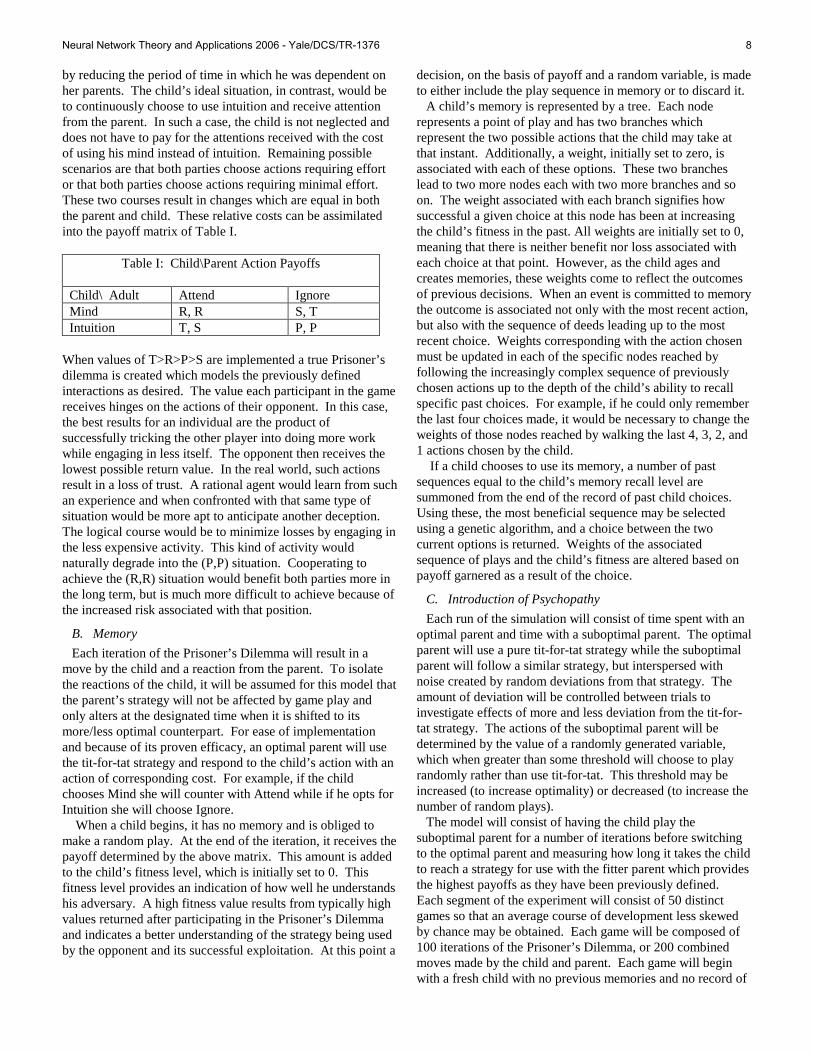
Results illustrate, as common sense would suggest, that both the quality and level of exposure to suboptimal caregivers is reflected in the child’s development. It is comforting, however, to realize that while consistent childcare is best for the development of a distinct, effective strategy on the part of the child, complete consistency is not necessary for its achievement. Rather, it seems that the consistency must simply outweigh the loss the child would expect by not conforming to the strategy being deviated from. This is a
necessary evolutionary development given that the overwhelming majority of parents would find it impossible to always behave fairly and in a tit-for-tat fashion throughout childhood. It is also interesting to note, that for the intent of the parent, a pure tit-for-tat strategy does not seem to be most advantageous when cost and resulting maturation are compared.
V. APPENDIX
Graph I
Graphs showing the average progression of fitness and Mind or maturity values in a situation in which a random agent is utilized for the first 50 iterations, after which an optimal (tit-for-tat) parent is substituted. Note the dramatic dip in fitness that occurs on the left at the point where the parents are exchanged. The child’s fitness decreases after the initial switch before rising steeply once more. The right demonstrates the sloping off of mind usage when exposed to a random agent followed by increased choosing of Mind in the presence of the optimal parent.
Neural Network Theory and Applications 2006 - Yale/DCS/TR-1376 12

Graph II
Both graphs illustrate the situation where a 30% optimal parent plays the first 50 iterations. However, on the left, this suboptimal parent is replaced by a parent who is 70% optimal while that on the right was replaced by an optimal parent. The increase in fitness is smoother and more dramatic on the right, but both demonstrate a definite improvement in the child’s fitness resulting from their respective changes.
Graph III
The top two illustrate the progression of a child’s fitness and maturity, as measured by the number of times they’ve chosen mind over the course of 100 iterations of the Prisoner’s Dilemma with a parent who randomly chooses actions while the bottom two are the results from interactions with a parent using tit-for-tat.
Neural Network Theory and Applications 2006 - Yale/DCS/TR-1376 13

VI. REFERENCES
[1] J. Logan, “A Game Theoretic and Genetic Algorithmic Approach to Modeling the Emergence of Mind in Early Child Development with Exposure to Semi-Developed Parents”.
[2] F. Happe “Theory of Mind and Self,” Annals of the New York Academy of Sciences, vol. 1001, Oct. 2003, pp 134.
[3] K. C. Pears, L. J. Moses, “Demographics, Parenting, and Theory of Mind in Preschool Children, “ Social Development, vol. 12, Feb. 2003, pp 1.
[4] J. Dunn, J. Brown, L. Beardsall, “Family Talk About Feeling States and Children’s Later Understandin of Others’ Emotions,” Developmental Psychology, vol. 27, May 1991, pp 448-455.
[5] L. Mayes, W. Miranker, “A Game Theoretic and Genetic Algorithmic Approach to Modeling the Emergence of Mind in Early Child Development,”
Neural Network Theory and Applications 2006 - Yale/DCS/TR-1376 14
Abstract—Self-organizing maps (also called Kohonen
networks) are a popular method of analyzing multidimensional data. In addition to compressing input data while preserving its topology, self-organizing maps can be used as a preliminary technique in cluster analysis. However, despite the fact that similar inputs remain close together in the output of the algorithm (suggesting possible clusters), no automatic segmentation of the data into discrete groups is provided. A variant of the SOM algorithm is proposed that dynamically clusters input data in an unsupervised fashion, automatically dividing the map into easily interpretable discrete submaps that correspond to clusters in the input data.
Index Terms—knowledge acquisition, neural networks, self-organizing feature maps, cluster analysis
I. INTRODUCTION
umans are capable of performing unsupervised categorization tasks, in which they distinguish between
and create categories around objects with which they have no prior experience. This process, called category construction in the literature on concepts and categorization (Murphy, [1]), is seen to occur quite frequently in children, and it is believed that children recognize objects as being in separate categories before they learn names for them (Merriman et al., [2]). Little is known about the precise mechanisms for how this is accomplished in humans, but being able to construct a system capable of simulating this behavior reliably would impact applications ranging from information storage and retrieval to object recognition and classification. One presumably important mechanism in such a system is the analysis of multidimensional data, such as might be received from input sensors or from the feature-based analysis of text, images, sound, or other information. Specifically, the creation of discrete categories from a data set would seem to require some method of clustering the data, such that coherent groups are formed that maximize the similarity of data within a group while minimizing the similarity between groups. Such clustering is formally the assignment of labels to vectors in the input. The number of labels that are assigned is equal to the number of clusters in the data. To mimic cognitive capabilities, this must proceed in an unsupervised manner. Thus it is necessary to discover algorithms capable of autonomously discovering clusters in a data set given minimal a priori information about the nature of the data set’s
distribution. Several statistical methods for clustering data exist and are widely used, however as these are not fully autonomous (requiring information regarding the expected number of clusters, and generally only capable of finding ellipsoidal clusters, cf. Costa and de Andrade Netto, [3]) they will not be reviewed here. Models of neural systems look to be a more promising path. Many such models are capable of unsupervised learning and organization, and furthermore most are inherently amenable to neurobiological accounts of the processes involved (i.e., they are psychologically plausible). In particular, the self-organizing map algorithm, developed by Teuvo Kohonen, has several properties that make it well suited for analyzing large amounts of multidimensional data with the goal of discovering natural groupings within that data. There have been clustering techniques that make use of the SOM algorithm; these will be discussed in section III below. After reviewing the relevant SOM-based approaches to cluster analysis and discussing some failed attempts at deriving autonomous cluster analysis tools, an algorithm is proposed that is capable of autonomously discovering clusters (including complex clusters with non-ellipsoidal shapes) by systematically adding and removing connections between units in the SOM, dynamically restructuring it in response to the underlying data distribution. In comparison with the traditional SOM algorithm, the proposed approach holds several advantages, including facilitated interpretation of the resulting map and better fit to the underlying data (as determined by visual inspection of the map).
II. THE SELF-ORGANIZING MAP ALGORITHM
A. Capabilities of the self-organizing map algorithm
Self-organizing maps (SOMs) are an effective tool in the analysis of multidimensional data. They are capable of converting high-dimensional data into a low-dimensional (often two-dimensional) representation that preserves the topological relations present in the primary data, in essence providing an estimation of the probability density function underlying the input data. SOMs have been widely used as tools to visualize high-dimensional data (Vesanto, [4]), and often act as guides in the exploratory phase of data mining (Vesanto and Alhoniemi, [5]). They have also been applied successfully in many natural language settings, having been shown to be capable of grouping words in a semantically meaningful way based on contextual information (Honkela et al., [6]). Furthermore, there is reason to believe that many of
Cluster Analysis with Dynamically Restructuring Self-Organizing Maps
Daniel Holtmann-Rice
H
Neural Network Theory and Applications 2006 - Yale/DCS/TR-1376 15
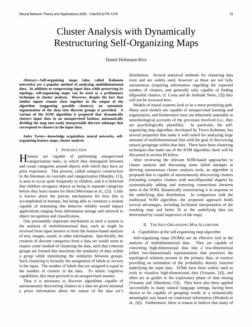
Fig. 1. The SOM algorithm with 49 neurons after 1000 iterations (well before convergence), on a two-dimensional input space. The grid-layout structure can be clearly seen. The black circles represent the neurons’ locations in weight space, with links between the neurons represented as lines connecting them. Light-gray circles represent the weight-space locations of previously presented input data. our own neurobiological subsystems may operate in ways similar to self-organizing maps. It has been shown (Ritter and Schulten, [7]) that SOM algorithms can successfully model sensory mappings and motor control functions, both of which are systems that the brain organizes topologically as well. Whether or not a SOM-based method for modeling aspects of the human conceptual system is feasible remains to be seen, but the place of SOM algorithms as effective knowledge representation devices is well established (Honkela, [8]).
B. The algorithm
A self-organizing map consists of a set of N neurons (also called units), each with l dimensional weight vectors that are initialized at random or from input data. Each neuron is “linked” to a number of other neurons (see Fig. 1) by a neighborhood relation that defines the structure of the map. (the choice of structure is rather flexible, a feature that will be exploited by the dynamic restructuring algorithm proposed in section IV). This linking is often done in such a way that the N neurons form a two-dimensional lattice – in this paper the SOM algorithm was implemented such that a two-dimensional grid of neurons was created, i.e. most neurons were linked to four other neurons (one in each direction, with the exception of neurons on the edges or corners of the grid). The set of neurons that a neuron is linked to is called its neighborhood.
The SOM algorithm proceeds iteratively, exposing the map to input data in the form of data vectors chosen with some probability from a data set. For each iteration, the algorithm proceeds as follows (refer to Haykin, [9], for a more in-depth analysis of the algorithm):
1. Select an input vector x at random from the data set.
2. Determine the “winning” neuron j whose weights are closest to the input vector in a Euclidean sense, i.e. the neuron whose weights wj are closest to x:
j =k
argmin x − wk
3. Update the weights of neurons in the map in a fashion
dependent upon their distance from neuron j. The distance dj,i between two neurons i and j is measured as the minimum number of links (as defined above) crossed when traversing the map from i to j. Let hj,i be a specified monotonic function that decreases with increasing d (in this paper the Gaussian function is used):
h j ,i(x) = exp(−d j ,i
2
2σ(t)2 )
where σ(t) is an exponentially decreasing function that specifies the size of a neuron’s topological neighborhood (intuitively, proportional to the extent of a neuron’s influence over other neurons during an iteration). Weights for a neuron i are then updated according to the following function: wi (t +1) = wi (t) + η(t) ⋅ h j ,i (t) ⋅ (x − w j (t))
where η(t) is a learning rate function that exponentially decreases with time.
This is continued for either a specified number of iterations or until a satisfactory level of convergence has been achieved.
III. USING THE SELF-ORGANIZING MAP ALGORITHM AS A
TOOL FOR CLUSTER ANALYSIS
The SOM algorithm does manage to maintain the topological relations of primary data quite well, resulting in a representation of the data where inputs that are close together (i.e. similar) in the primary data remain close together in the SOM. However, there is no immediate way of recognizing whether discrete clusters (“classes”) of points are present in the data (and if so, how many) using solely the SOM algorithm. Furthermore, when presented with data that is not contiguous throughout weight space (as in Fig. 1, where the data is clearly composed of eight discrete regions), the SOM algorithm does a mediocre job of approximating the data distribution (Fig. 2), despite the fact that this is precisely the sort of data one would expect a clustering algorithm to have no difficulty with. Some neurons (“interpolating map units”) converge to locations in between clusters of data points,
Neural Network Theory and Applications 2006 - Yale/DCS/TR-1376 16
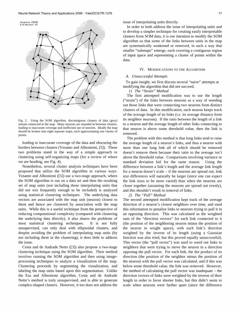
Fig. 2. Using the SOM algorithm, discontiguous clusters of data (grey) remain connected in the map. Many neurons are stranded in between clusters, leading to inaccurate coverage and inefficient use of neurons. Ideally the map should be broken into eight separate maps, each approximating one cluster of points.
leading to inaccurate coverage of the data and obscuring the borders between clusters (Vesanto and Alhoniemi, [5]). These two problems stand in the way of a simple approach to clustering using self-organizing maps (for a review of where we are heading, see Fig. 4).
Nonetheless, several cluster analysis techniques have been proposed that utilize the SOM algorithm in various ways. Vesanto and Alhoniemi ([5]) use a two-stage approach, where the SOM algorithm is run on a data set and then the resulting set of map units (not including those interpolating units that did not win frequently enough to be included) is analyzed using statistical clustering techniques. The underlying data vectors are associated with the map unit (neuron) closest to them and hence are clustered by association with the map units. While this is a useful technique from the perspective of reducing computational complexity (compared with clustering the underlying data directly), it also shares the problems of most statistical clustering techniques. It is not fully unsupervised, can only deal with ellipsoidal clusters, and despite avoiding the problem of interpolating map units (by not including them in the clustering), it does little to address the issue.
Costa and de Andrade Netto ([3]) also propose a two-stage clustering technique using the SOM algorithm. Their method involves running the SOM algorithm and then using image-processing techniques to analyze a visualization of the map. Clustering proceeds by segmenting the visualization, and labeling the map units based upon this segmentation. Unlike the Esa and Alhoniemi algorithm, Costa and de Andrade Netto’s method is truly unsupervised, and is able to generate complex-shaped clusters. However, it too does not address the
issue of interpolating units directly. In order to both address the issue of interpolating units and
to develop a simpler technique for creating easily interpretable clusters from SOM data, it is our intention to modify the SOM algorithm so that some of the links between units in the map are systematically weakened or removed, in such a way that smaller “submaps” emerge, each covering a contiguous region of input space and representing a cluster of points within the data.
IV. MODIFICATIONS TO THE ALGORITHM
A. Unsuccessful Attempts
To gain insight, we first discuss several “naive” attempts at modifying the algorithm that did not succeed.
1) The “Strain” Method The first attempted modification was to use the length
(“strain”) of the links between neurons as a way of weeding out those links that were connecting two neurons from distinct clusters of data. In this modification, each neuron keeps track of the average length of its links (i.e. its average distance from its neighbor neurons). If the ratio between the length of a link to a neuron and the average length of other links connecting to that neuron is above some threshold value, then the link is removed.
The problem with this method is that long links tend to raise the average length of a neuron’s links, and thus a neuron with more than one long link all of which should be removed doesn’t remove them because their ratio to the average isn’t above the threshold value. Comparisons involving variance or standard deviation fail for the same reason. Using the difference between a link’s length and the average link length for a neuron doesn’t scale – if the neurons are spread out, link size differences will naturally be larger (since one can expect the link sizes to be more varied) than when the neurons are closer together (assuming the neurons are spread out evenly), and this shouldn’t result in removal of links.
2) The “Pull” Method The second attempted modification kept track of the average direction of a neuron’s closest neighbors over time, and used this information to penalize links to neurons trying to pull it in an opposing direction. This was calculated as the weighted sum of the “direction vectors” for each link connected to it (the position of the neighboring neuron minus the position of the neuron in weight space), with each link’s direction weighted by the inverse of its length (using a Gaussian function was also tried, but this proved equally unsuccessful). This vector (the “pull vector”) was used to weed out links to neighbors that were trying to move the neuron in a direction opposing the pull vector. For each link, the dot product of its direction (the position of the neighbor minus the position of the neuron) with the pull vector was calculated, and if this was below some threshold value, the link was removed. However, the method of calculating the pull vector was inadequate – the direction vectors of links were weighted by the inverse of their length in order to favor shorter links, but this didn’t seem to scale when neurons were farther apart (since the difference
Neural Network Theory and Applications 2006 - Yale/DCS/TR-1376 17
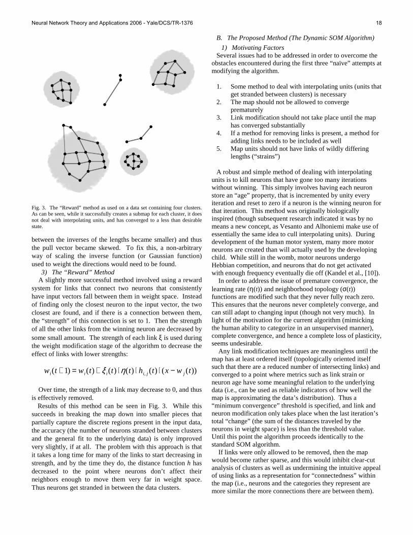
Fig. 3. The “Reward” method as used on a data set containing four clusters. As can be seen, while it successfully creates a submap for each cluster, it does not deal with interpolating units, and has converged to a less than desirable state. between the inverses of the lengths became smaller) and thus the pull vector became skewed. To fix this, a non-arbitrary way of scaling the inverse function (or Gaussian function) used to weight the directions would need to be found.
3) The “Reward” Method A slightly more successful method involved using a reward
system for links that connect two neurons that consistently have input vectors fall between them in weight space. Instead of finding only the closest neuron to the input vector, the two closest are found, and if there is a connection between them, the “strength” of this connection is set to 1. Then the strength of all the other links from the winning neuron are decreased by some small amount. The strength of each link ξ is used during the weight modification stage of the algorithm to decrease the effect of links with lower strengths:
wi (t +1) = wi (t) + ξ i (t) ⋅η(t) ⋅ hi, j (t) ⋅ (x − w j (t))
Over time, the strength of a link may decrease to 0, and thus
is effectively removed. Results of this method can be seen in Fig. 3. While this
succeeds in breaking the map down into smaller pieces that partially capture the discrete regions present in the input data, the accuracy (the number of neurons stranded between clusters and the general fit to the underlying data) is only improved very slightly, if at all. The problem with this approach is that it takes a long time for many of the links to start decreasing in strength, and by the time they do, the distance function h has decreased to the point where neurons don’t affect their neighbors enough to move them very far in weight space. Thus neurons get stranded in between the data clusters.
B. The Proposed Method (The Dynamic SOM Algorithm)
1) Motivating Factors Several issues had to be addressed in order to overcome the
obstacles encountered during the first three “naïve” attempts at modifying the algorithm.
1. Some method to deal with interpolating units (units that
get stranded between clusters) is necessary 2. The map should not be allowed to converge
prematurely 3. Link modification should not take place until the map
has converged substantially 4. If a method for removing links is present, a method for
adding links needs to be included as well 5. Map units should not have links of wildly differing
lengths (“strains”) A robust and simple method of dealing with interpolating
units is to kill neurons that have gone too many iterations without winning. This simply involves having each neuron store an “age” property, that is incremented by unity every iteration and reset to zero if a neuron is the winning neuron for that iteration. This method was originally biologically inspired (though subsequent research indicated it was by no means a new concept, as Vesanto and Alhoniemi make use of essentially the same idea to cull interpolating units). During development of the human motor system, many more motor neurons are created than will actually used by the developing child. While still in the womb, motor neurons undergo Hebbian competition, and neurons that do not get activated with enough frequency eventually die off (Kandel et al., [10]). In order to address the issue of premature convergence, the learning rate (η(t)) and neighborhood topology (σ(t)) functions are modified such that they never fully reach zero. This ensures that the neurons never completely converge, and can still adapt to changing input (though not very much). In light of the motivation for the current algorithm (mimicking the human ability to categorize in an unsupervised manner), complete convergence, and hence a complete loss of plasticity, seems undesirable. Any link modification techniques are meaningless until the map has at least ordered itself (topologically oriented itself such that there are a reduced number of intersecting links) and converged to a point where metrics such as link strain or neuron age have some meaningful relation to the underlying data (i.e., can be used as reliable indicators of how well the map is approximating the data’s distribution). Thus a “minimum convergence” threshold is specified, and link and neuron modification only takes place when the last iteration’s total “change” (the sum of the distances traveled by the neurons in weight space) is less than the threshold value. Until this point the algorithm proceeds identically to the standard SOM algorithm. If links were only allowed to be removed, then the map would become rather sparse, and this would inhibit clear-cut analysis of clusters as well as undermining the intuitive appeal of using links as a representation for “connectedness” within the map (i.e., neurons and the categories they represent are more similar the more connections there are between them).
Neural Network Theory and Applications 2006 - Yale/DCS/TR-1376 18
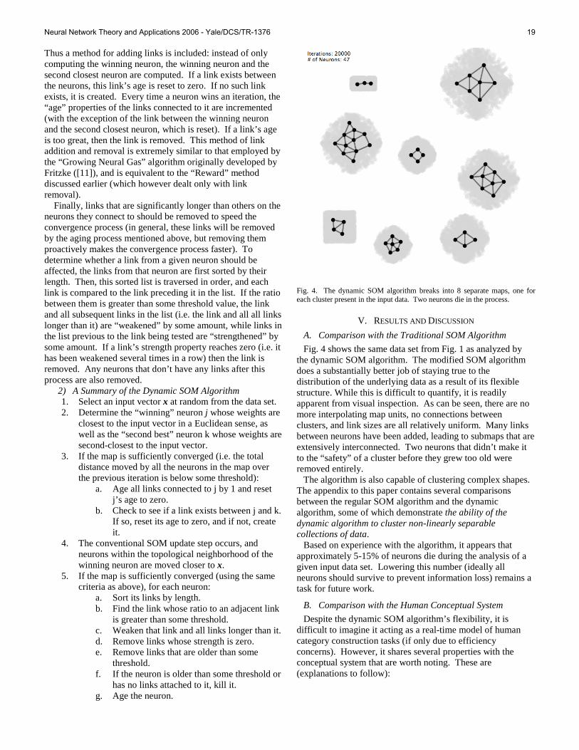
Thus a method for adding links is included: instead of only computing the winning neuron, the winning neuron and the second closest neuron are computed. If a link exists between the neurons, this link’s age is reset to zero. If no such link exists, it is created. Every time a neuron wins an iteration, the “age” properties of the links connected to it are incremented (with the exception of the link between the winning neuron and the second closest neuron, which is reset). If a link’s age is too great, then the link is removed. This method of link addition and removal is extremely similar to that employed by the “Growing Neural Gas” algorithm originally developed by Fritzke ([11]), and is equivalent to the “Reward” method discussed earlier (which however dealt only with link removal). Finally, links that are significantly longer than others on the neurons they connect to should be removed to speed the convergence process (in general, these links will be removed by the aging process mentioned above, but removing them proactively makes the convergence process faster). To determine whether a link from a given neuron should be affected, the links from that neuron are first sorted by their length. Then, this sorted list is traversed in order, and each link is compared to the link preceding it in the list. If the ratio between them is greater than some threshold value, the link and all subsequent links in the list (i.e. the link and all all links longer than it) are “weakened” by some amount, while links in the list previous to the link being tested are “strengthened” by some amount. If a link’s strength property reaches zero (i.e. it has been weakened several times in a row) then the link is removed. Any neurons that don’t have any links after this process are also removed.
2) A Summary of the Dynamic SOM Algorithm 1. Select an input vector x at random from the data set. 2. Determine the “winning” neuron j whose weights are
closest to the input vector in a Euclidean sense, as well as the “second best” neuron k whose weights are second-closest to the input vector.
3. If the map is sufficiently converged (i.e. the total distance moved by all the neurons in the map over the previous iteration is below some threshold):
a. Age all links connected to j by 1 and reset j’s age to zero.
b. Check to see if a link exists between j and k. If so, reset its age to zero, and if not, create it.
4. The conventional SOM update step occurs, and neurons within the topological neighborhood of the winning neuron are moved closer to x.
5. If the map is sufficiently converged (using the same criteria as above), for each neuron:
a. Sort its links by length. b. Find the link whose ratio to an adjacent link
is greater than some threshold. c. Weaken that link and all links longer than it. d. Remove links whose strength is zero. e. Remove links that are older than some
threshold. f. If the neuron is older than some threshold or
has no links attached to it, kill it. g. Age the neuron.
Fig. 4. The dynamic SOM algorithm breaks into 8 separate maps, one for each cluster present in the input data. Two neurons die in the process.
V. RESULTS AND DISCUSSION
A. Comparison with the Traditional SOM Algorithm
Fig. 4 shows the same data set from Fig. 1 as analyzed by the dynamic SOM algorithm. The modified SOM algorithm does a substantially better job of staying true to the distribution of the underlying data as a result of its flexible structure. While this is difficult to quantify, it is readily apparent from visual inspection. As can be seen, there are no more interpolating map units, no connections between clusters, and link sizes are all relatively uniform. Many links between neurons have been added, leading to submaps that are extensively interconnected. Two neurons that didn’t make it to the “safety” of a cluster before they grew too old were removed entirely.
The algorithm is also capable of clustering complex shapes. The appendix to this paper contains several comparisons between the regular SOM algorithm and the dynamic algorithm, some of which demonstrate the ability of the dynamic algorithm to cluster non-linearly separable collections of data.
Based on experience with the algorithm, it appears that approximately 5-15% of neurons die during the analysis of a given input data set. Lowering this number (ideally all neurons should survive to prevent information loss) remains a task for future work.
B. Comparison with the Human Conceptual System
Despite the dynamic SOM algorithm’s flexibility, it is difficult to imagine it acting as a real-time model of human category construction tasks (if only due to efficiency concerns). However, it shares several properties with the conceptual system that are worth noting. These are (explanations to follow):
Neural Network Theory and Applications 2006 - Yale/DCS/TR-1376 19

1. It functions as a cross between exemplar and prototype models of category representation.
2. Active “perception” in a specific area of weight-space changes representation of that area of weight-space.
3. It functions by viewing only one piece of input data at a time, much as we do (with selective attention).
1. Two approaches to category representation exist in the
concepts and categories literature (Murphy, [1]). The “exemplar view” holds that we store every memory of things we’ve encountered that belong to a certain category. When we categorize a novel object, we compare that object to every exemplar we have stored in memory, and choose the most similar exemplars for use in categorizing the object. The opposing view is that we “average” our interactions with category members to arrive at an “idealized” category member – a prototypical member of the category. The SOM algorithm represents clusters using what could be viewed as a set of multiple prototypes. This is not as memory intensive as the exemplar approach, and not as limiting from a representational standpoint as the prototype approach.
2. It is reasonable to assume that our representation of a concept only changes when we interact with or think about instances of that concept (or very similar concepts). This is similar to the SOM algorithm, since there is a limit to the influence of an input vector – it only affects the neurons closest to it.
3. When we interact with objects in the world, we interact with them generally one at a time. Thus, whatever system we have for learning and organizing our conceptual knowledge must operate on minimal input, i.e., it can function without knowing a priori the size, distribution, and frequency of a category – it can learn based on seeing only one instance of that category at a time. The SOM algorithm operates on similar principles.
Finally, one aspect of the SOM algorithm as implemented here that differs substantially from human conceptual experience is the lack of temporal continuity with respect to input. When we walk into a room, we are faced with the same set of objects for an extended period of time. This is not the case with the SOM algorithm, where input data is selected randomly, and there is no reliable relation between one input vector and the next.
C. Remaining Problems and Future Work
Several problems with the dynamic SOM algorithm remain. Clusters must be spaced rather far apart in order for the algorithm to detect them and not treat them as contiguous regions of input data. There is an inverse relationship between the number of neurons in the map and the minimum separation between clusters that must be present in order for clusters to be accurately identified – more neurons in the map makes the spacing between neurons smaller, which means links between clusters are less likely to be activated.
The algorithm is also slow. Due to the similarity between this algorithm and the growing neural gas algorithm, it would thus be desirable to do a direct comparison between the two to see which converges faster.
Finally, the algorithm has not yet been tested on real-world data. It remains to be seen whether it can accurately and
meaningfully detect clusters in multidimensional real-world data, however the preliminary results from synthetic data are promising.
REFERENCES [1] Murphy, G. The Big Book of Concepts, Cambridge, MA: MIT Press,
2002. [2] Merriman, W. E., Schuster, J. M., and Hager, L. (1991) Are names ever
mapped onto pre-existing categories. Journal of Experimental Psychology: General, 120, 288-300.
[3] Costa, J.A.F.; de Andrade Netto, M.L., (1999) Cluster analysis using self-organizing maps and image processing techniques. IEEE International Conference on Systems, Man, and Cybernetics, 1999, vol. 5, pp. 367-372.
[4] Vesanto, J. (1999) SOM-based data visualization methods. Intelligent Data Analysis, vol. 3, pp. 111–126.
[5] Vesanto, J. and Alhoniemi, E. (2000) Clustering of the Self-Organizing Map. IEEE Transactions on Neural Networks, vol. 11, no. 3, pp. 586-600.
[6] Honkela, T., Pulkki, V., & Kohonen, T. (1995) Contextual Relations of Words in Grimm Tales Analyzed by Self-Organizing Map. Proceedings of ICANN-95, International Conference on Artificial Neural Networks, vol. 2, F. Fogelman-Soulié and P. Gallinari (eds.), EC2 et Cie, Paris, pp. 3-7.
[7] Ritter, H. J. and Schulten, K. (1988) Kohonen's self-organizing maps: Exploring their computational capabilities, In: Proc. IEEE Int. Conf. Neural Network, ICNN-88, San Diego, CA, pp. 109-116.
[8] Honkela T. (2000) Adaptive and Holistic Knowledge Representations Using Self-Organizing Maps. Proceedings of IIP'2000, International Conference on Intelligent Information Processing, Z. Shi, B. Faltings and M. Musen (eds.), Beijing, China, August 21-25, 2000, pp. 81-86.
[9] S. Haykin, Neural networks: A comprehensive foundation, Upper Saddle River, NJ: Prentice-Hall, 1994.
[10] Kandel, E. R., Schwartz, J. H., Jessell, T. M. Principles of Neural Science, 4th Edition, Chicago, IL: The Unviersity of Chicago Press, 2000.
[11] Fritzke, B. (1995) A Growing Neural Gas Network Learns Topologies, in: Tesauro, G., Touretzky, D. S., Leen, T. K. (Eds.): Advances in Neural Information Processing Systems 7, MIT Press, 625-632.
Neural Network Theory and Applications 2006 - Yale/DCS/TR-1376 20
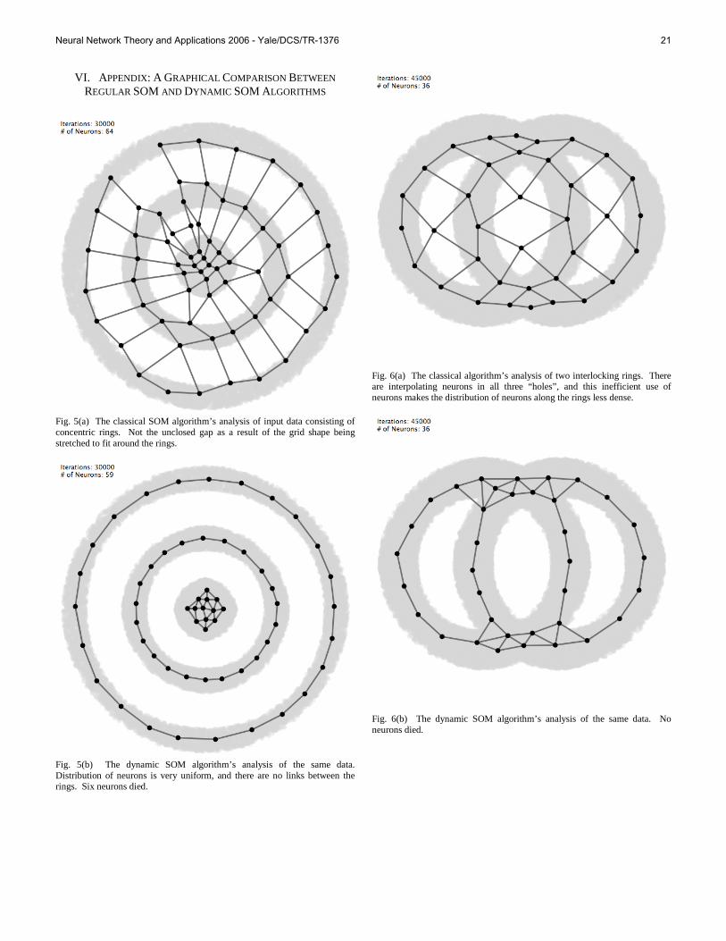
VI. APPENDIX: A GRAPHICAL COMPARISON BETWEEN
REGULAR SOM AND DYNAMIC SOM ALGORITHMS
Fig. 5(a) The classical SOM algorithm’s analysis of input data consisting of concentric rings. Not the unclosed gap as a result of the grid shape being stretched to fit around the rings.
Fig. 5(b) The dynamic SOM algorithm’s analysis of the same data. Distribution of neurons is very uniform, and there are no links between the rings. Six neurons died.
Fig. 6(a) The classical algorithm’s analysis of two interlocking rings. There are interpolating neurons in all three “holes”, and this inefficient use of neurons makes the distribution of neurons along the rings less dense.
Fig. 6(b) The dynamic SOM algorithm’s analysis of the same data. No neurons died.
Neural Network Theory and Applications 2006 - Yale/DCS/TR-1376 21
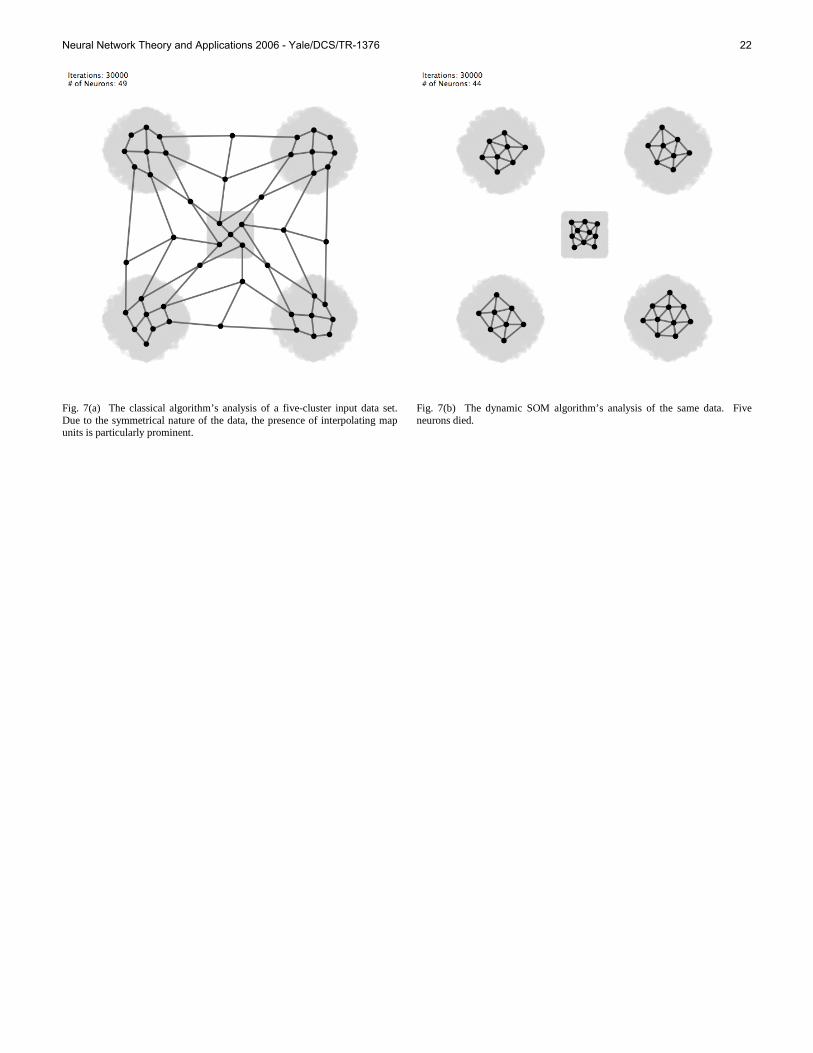
Fig. 7(a) The classical algorithm’s analysis of a five-cluster input data set. Due to the symmetrical nature of the data, the presence of interpolating map units is particularly prominent.
Fig. 7(b) The dynamic SOM algorithm’s analysis of the same data. Five neurons died.
Neural Network Theory and Applications 2006 - Yale/DCS/TR-1376 22

Neural Network Theory and Applications 2006 1
Abstract—With customer preference databases growing to
colossal sizes, collaborative filtering algorithms run into scalability concerns. By reducing the dimensionality of the input space, we ease the demands of predicting users’ tastes for films. A movie-to-movie correlation and distance metric are used to decompose the user-movie rating data into two different movie graphs. Using a Kohonen self-organizing map (SOM), the product space can be divided into meaningful clusters centered on the neurons whose weight vectors are nearest the product weights. The SOM –derived clustering is analyzed via a Principal Components Analysis of the data. The clusterings are then evaluated for their effectiveness via quantitative and qualitative observations on the meaningfulness of the groupings of the films.
Index Terms—Clustering methods, Collaborative filtering, Karhunen-Loeve transforms, Movies, Neural network applications, Self-organizing feature maps
I. INTRODUCTION OLLABORATIVE filtering, the automated process of making predictions about a user’s interests given
data collected on customers’ prior preferences, has become an increasingly relevant problem. Mindful companies are cataloging their customers’ every move, hoping to uncover meaningful trends that help refocus product selection and marketing. Collaborative filtering need not only be seen as an aid to the seller, however; customers, who are more regularly inundated by an increasingly complicated market with thousands of slightly differentiated products, benefit highly from individualized product suggestions. The substantial size of the customer preference databases (the inputs for collaborative filtering) makes the problem of individualizing the recommendation process even more difficult [6]. Collaborative filtering techniques generally fall into two groups by the type of approach, either memory-based or model-based algorithms. The former make determinations according to an analysis of the entire dataset whereas the latter fine-tune a user-specific model designed to capture an individual’s relationship to the entire product space.
Each approach presents difficulties when scalability is a concern [6]. This paper proposes dimensionality reduction via product clustering as a solution to the problem of scalability. The product space—here, the set of all films—when partitioned, becomes more manageable for calculations. In the same way that the human brain generates classification schema to aid in comprehending the world [1], collaborative filtering algorithms can consider a user’s relationship to these categories (instead of looking at the user’s relationship to each individual item independently) [5]. The partitioning of the product space is accomplished by training a Kohonen self-organizing map on relational film data. The resulting clusters are analyzed and then graphed via a principal components analysis. It is hard to quantitatively measure the partitions that emerge, though data on the films’ genres, directors contribute to a qualitative assessment of the clustering algorithm. The clusters derived from the self-organizing map are by no means perfect, though the similarity between the films in each partition is no accident. In almost every partitioning of the films, movies end up in the same clusters as their sequels (with the noted exception of the Harry Potter franchise, where the third and fourth films are markedly different than the first and second, both sets of which are grouped in different clusters). Most clusters seem to exhibit some property that differentiates the films in the particular group from the entire set of all movies being considered, be it genre, budget, director style, or some more subjective quality.
Indeed, the quality of the partitions is impressive considering the amount of data that is aggregated to arrive at the results. This suggests that SOM algorithms like this one may provide the key to developing collaborative filtering systems in the face of increasing scalability concerns.
II. THE NETFLIX PRIZE™ DATA Netflix provides the following as description of its data: “The movie rating files contain over 100 million ratings from
A. Pariser is a senior at Yale University, expecting graduation with a BS in
May of 2007 for a Physics and Applied Mathematics double major, (e-mail: [email protected]).
Dimensionality Reduction via Self-Organizing Feature Maps for Collaborative Filtering
Andrew R. Pariser
C
Neural Network Theory and Applications 2006 - Yale/DCS/TR-1376 23

Neural Network Theory and Applications 2006 2
480 thousand randomly-chosen, anonymous Netflix customers over 17 thousand movie titles. The data were collected between October, 1998 and December, 2005 and reflect the distribution of all ratings received during this period. The ratings are on a scale from 1 to 5 (integral) stars. To protect customer privacy, each customer id has been replaced with a randomly-assigned id. The date of each rating and the title and year of release for each movie id are also provided.” The five hundred most rated movies were extracted from this dataset for the tests that follow, representing a meaningful portion of the entire population of ratings while keeping computation time reasonable. These films comprise the product space of this research.
III. TASTE PROFILE DECOMPOSITION
A. Overview It is difficult to find a basis on which one can partition
the set of viewer-movie rating pairs. Instead, one would intuitively think to create groupings among either the set of movies or the set of users. A cluster from the set of users would hopefully contain customers who would rank movies similarly. Likewise, a cluster from the set of movies would ideally collect all titles which will probably receive the same ratings across all users.
The goal of this first step is to transform the viewer-movie rating pairs into data that relate the films via some calculation on collective ratings data, simplifying hundreds of user ratings for two films into one value.
B. Movie-Movie Metrics In order to transform the user-movie rating pairs into a
relational graph of movies, we must aggregate the user data via some metric that relates two movies. We consider two such measures, a correlation metric and a distance metric.
Let U(m) represent the set of all users who have rated movie m. We define U(m,n) = U(m) ∩ U(n) as the set of users who have rated both movies m and n. Using the variable u to represent a user, we define rm(u), mm, and sm as the rating user u gives movie m, the mean rating for movie m, and the standard deviation of all users’ ratings for movie m, respectively. We then consider the functions
1 2( , )
( ) ( ( ) ) ( ( ) )mn m n m m n nu U m nr u r uρ σ σ μ μ−
∈= − −∑ (1)
and
2( , )
( ( ) ( ))mn m nu U m nd r u r u
∈= −∑ (2)
where (1) represents a measure of correlation and (2) a measure of distance between m and n.
The resulting data from equations (1) and (2) are then
normalized so that –1 ≤ rmn ≤ 1 and 0 ≤ dmn ≤ 1. To sharpen the metrics and to aid in providing clearer boundaries on which to cluster the graphs, we exponentiate the results of the two formulae above, obtaining
exp( )mn mnρ ρ′ = − (3)
and
exp( )mn mnd d′ = − . (4)
The bounds on (3) and (4) are 0.368 ≤ r'mn ≤ 2.718 and 0.368 ≤ d'mn ≤ 1, and are determined by transforming the bounds on (1) and (2).
The values from (3) and (4) are compiled into two matrices, R = (r'mn) and D = (d'mn).The columns of these two matrices, which we denote Rm and Dm respectively, correspond to vectors in the input space of the system. The elements in each vector define the particular movie in relation to the other films via the relational metrics in (3) and (4).
That the 500 most rated Netflix films were extracted from all movies provided in the dataset proved useful not only for computation time. Equations (1) and (2), which relate two films, depend upon having a non-empty intersection U(m,n) = U(m) ∩ U(n). It would be unclear how to speak of a “correlation” or “distance” between two products if one could not find a common subset of users who have provided taste profiles on both products. Thankfully, when limiting the data to the top 500 most rated films, the size of the intersection, |U(m,n)|, is strictly positive and thus Equations (1) – (4) are always defined.
An introductory analysis of the 500 most rated Netflix films is compiled in Appendix A. It includes lists of the ten most rated films, the ten films with highest and lowest ratings, and the ten films with highest and lowest variance in their ratings. Additionally, insight into the metrics of Equations (1) and (2) is provided by listing the ten most and least correlated films, as well as the ten most and least distant films.
IV. CLUSTERING VIA SELF-ORGANIZING MAP
A. Definition and Motivation Self-organizing maps (SOMs) distinguish features from an input space by forming topographical representations of their input patterns. Using competitive learning, “winning” neurons (and their neighbors) adjust their weight vectors to move closer to presented inputs (the columns of R and D) in synaptic weight space. After a convergence phase, the resulting neuron assembly exhibits important properties of the input space [2]:
Neural Network Theory and Applications 2006 - Yale/DCS/TR-1376 24

Neural Network Theory and Applications 2006 3
1. The feature map, as represented by the set of synaptic weight vectors, approximates the entire input space
2. The feature map is topologically ordered. That is, the spatial locations of the neurons represent a particular feature or subset of the input space.
3. The neuron density of the resulting feature map mimics the probability density of the input space.
4. As a conclusion of the previous three properties, a self-organizing map is able to select a set of best features for approximating an underlying distribution.
Given these four properties, one can easily assign clusters to movies from a particular SOM network: for each movie in the input space, it belongs in the cluster corresponding to the neuron nearest it in weight space.
B. Specification of SOM model and parameters Two SOMs are trained on each of the input spaces
defined by the sets of column vectors {Rm} and {Dm}, one with N neurons, both for N = 10 and N = 30. The output, therefore, corresponds to four different clusterings, one for ten clusters of each input space and the other of thirty clusters of each input space.
In these four clusterings, the synaptic weight space for each network is [0.368, 2.718]500 and [0.368, 1]500, for Rm and Dm, respectively. The initial synaptic weights for the fifty neurons are chosen randomly from the sets {Rm} and {Dm}.
At each iteration n of the network training phase, an input vector x(n) is presented to the network, where the input vector is given by a column vector of R or D, allof which are presented in a randomly permuted order in each training epoch. Competitive learning is used such that a best-matching (winning) neuron i(x) is chosen according to the minimum-distance criterion:
{1,2, , }
( ) arg min ( ) jj N
i n∈
= −x x w…
The winning neuron moves its weights in the direction of the input presentation x according to the update formula
, ( )( 1) ( ) ( ) ( ) ( ( ) ( ))j j j i jn n n h n n nη+ = + −xw w x w ,
where the learning rate function is defined by
0( ) exp ( / )n nη η τ= − ,
and the neighborhood function is defined to be the Kroniker delta function
,
1 if ( )
0 otherwisei j ij
i jh n δ
=⎧= = ⎨
⎩.
Choosing the particular parameters for these functions affects the speed and accuracy of the network training algorithm. Making h(n) ineffective by starting h0 too low may trap the network in local minima, whereas choosing h0 too high can cause the network to exhibit unfortunate oscillatory behavior. Similarly, these same effects can be achieved by changing the exponential decay of h(n) improperly; the network may overshoot optimal regions when t set too high, whereas, if t is set too low, the network will converge very slowly if at all.
C. Choosing Network Training Parameters The learning rate parameters h0 = 0.01 and t = 1000
are suggested by Haykin [2]. In selecting these parameters, one would hope to find the minimum value for the total self organizing map error as a function of the network’s weights W given by
2500
( )1( ) total_net_error ( )
ji jj =≡ = −∑ xW W W x . (5)
Here, the input vectors {x1, …, x500} correspond to the column vectors {Rm} and {Dm} as the case may be, and the term ( )ji xW symbolizes the weight vector of the best-matching (winning) neuron i(xj) for the given input vector xj. Once each network has been sufficiently trained, this value in (5) no longer decreases.
For each matrix and each number of output clusters, multiple values for each of the network training parameters h0 and t were compared according to their ability to minimize this error (w).
Tables 1 and 2 show results from these calculations. Shaded rows in each table correspond to parameter choices producing the lowest final values of the error found. The values for h0 and t for the actual training of each network were read directly from these shaded rows. Table 1 – Optimal Parameters, R-Network Training
10 Clusters, R 30 Clusters, R h0 t h0 t
0.9389 0.1 250 0.8856 0.1 250 0.9314 0.1 500 0.8683 0.1 500 0.9302 0.1 750 0.8606 0.1 750 0.9299 0.1 1000 0.8578 0.1 1000 0.9334 0.2 250 0.8656 0.2 250 0.9267 0.2 500 0.8563 0.2 500 0.9264 0.2 750 0.8486 0.2 750 0.9238 0.2 1000 0.8509 0.2 1000 0.9304 0.3 250 0.8593 0.3 250 0.9245 0.3 500 0.8489 0.3 500 0.9259 0.3 750 0.8429 0.3 750 0.9227 0.3 1000 0.8439 0.3 1000
Neural Network Theory and Applications 2006 - Yale/DCS/TR-1376 25
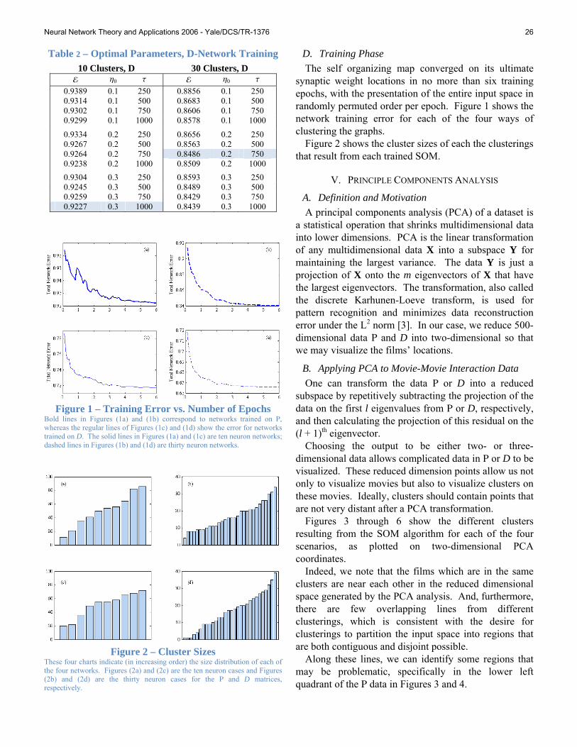
Neural Network Theory and Applications 2006 4
Table 2 – Optimal Parameters, D-Network Training 10 Clusters, D 30 Clusters, D h0 t h0 t
0.9389 0.1 250 0.8856 0.1 250 0.9314 0.1 500 0.8683 0.1 500 0.9302 0.1 750 0.8606 0.1 750 0.9299 0.1 1000 0.8578 0.1 1000
0.9334 0.2 250 0.8656 0.2 250 0.9267 0.2 500 0.8563 0.2 500 0.9264 0.2 750 0.8486 0.2 750 0.9238 0.2 1000 0.8509 0.2 1000 0.9304 0.3 250 0.8593 0.3 250 0.9245 0.3 500 0.8489 0.3 500 0.9259 0.3 750 0.8429 0.3 750 0.9227 0.3 1000 0.8439 0.3 1000
Figure 1 – Training Error vs. Number of Epochs
Bold lines in Figures (1a) and (1b) correspond to networks trained on R, whereas the regular lines of Figures (1c) and (1d) show the error for networks trained on D. The solid lines in Figures (1a) and (1c) are ten neuron networks; dashed lines in Figures (1b) and (1d) are thirty neuron networks.
Figure 2 – Cluster Sizes
These four charts indicate (in increasing order) the size distribution of each of the four networks. Figures (2a) and (2c) are the ten neuron cases and Figures (2b) and (2d) are the thirty neuron cases for the R and D matrices, respectively.
D. Training Phase The self organizing map converged on its ultimate
synaptic weight locations in no more than six training epochs, with the presentation of the entire input space in randomly permuted order per epoch. Figure 1 shows the network training error for each of the four ways of clustering the graphs.
Figure 2 shows the cluster sizes of each the clusterings that result from each trained SOM.
V. PRINCIPLE COMPONENTS ANALYSIS
A. Definition and Motivation A principal components analysis (PCA) of a dataset is
a statistical operation that shrinks multidimensional data into lower dimensions. PCA is the linear transformation of any multidimensional data X into a subspace Y for maintaining the largest variance. The data Y is just a projection of X onto the m eigenvectors of X that have the largest eigenvectors. The transformation, also called the discrete Karhunen-Loeve transform, is used for pattern recognition and minimizes data reconstruction error under the L2 norm [3]. In our case, we reduce 500-dimensional data R and D into two-dimensional so that we may visualize the films’ locations.
B. Applying PCA to Movie-Movie Interaction Data One can transform the data R or D into a reduced
subspace by repetitively subtracting the projection of the data on the first l eigenvalues from R or D, respectively, and then calculating the projection of this residual on the (l + 1)th eigenvector.
Choosing the output to be either two- or three-dimensional data allows complicated data in R or D to be visualized. These reduced dimension points allow us not only to visualize movies but also to visualize clusters on these movies. Ideally, clusters should contain points that are not very distant after a PCA transformation.
Figures 3 through 6 show the different clusters resulting from the SOM algorithm for each of the four scenarios, as plotted on two-dimensional PCA coordinates.
Indeed, we note that the films which are in the same clusters are near each other in the reduced dimensional space generated by the PCA analysis. And, furthermore, there are few overlapping lines from different clusterings, which is consistent with the desire for clusterings to partition the input space into regions that are both contiguous and disjoint possible.
Along these lines, we can identify some regions that may be problematic, specifically in the lower left quadrant of the R data in Figures 3 and 4.
Neural Network Theory and Applications 2006 - Yale/DCS/TR-1376 26

Neural Network Theory and Applications 2006 5
Figure 3 – Ten-Clustering of R Data
Figure 4 – Thirty-Clustering of R Data
Figure 5 – Ten-Clustering of D Data
Figure 6 – Thirty-Clustering of D Data
VI. QUALITATIVE ANALYSIS OF PARTITIONS
A. Introduction What sort of metric can be used to quantitatively say
that a clustering of films is meaningful? One can only do this when using some measure of “closeness” between films. Having defined two such measures (r'mn and d'mn) in the decomposition step (see III) and used these values as inputs to our clustering algorithm, it would be tautological to say that the clusters we have created are successful partitions with respect to these metrics. Supposing the metrics used for decomposition are poor indicators of the film “closeness,” our analysis would not observe poor clusterings of the data.
As such, we must look to a qualitative analysis of the film partitions. To do this, data from the Internet Movie Database (IMDB) were collected for each of the films in the product space. The average rating, budget, opening weekend gross, MPAA rating (i.e., R, PG-13, etc.), genres, directors, writers, and cast were then aggregated for each cluster as a means for qualitative comparison of the partitions.
B. Example Clusters First, we will look at a cluster that provides a sanity
check and reveals that the SOM methodology above generates at least some meaningful partitions. Example Cluster 1 (text box, next page) contains only eleven films, which is significantly fewer than 50, the average cluster size with ten partitions on 500 films. The extremely small size of the partition as compared to the average cluster size means that these eleven films must be very closely related and highly distinct from the other films in the product space.
Indeed, we see that six of these films are from the Lord of the Rings franchise (three Extended Edition DVD releases and three theatrical versions). The other films are also epic films, which are similar in scope and extravagance (not to mention, in length).
The average budget for these eleven films is on the high end of all clusterings at 73 million USD. The budgets of this cluster also have a low variance of 41 million dollars (relative to the budget size and compared to the other clusterings’ budget variance) which can be accounted for by the change in value of the dollar since the Star Wars films came out.
These films were made to be giant blockbusters. All had extremely high opening weekend gross revenues, and these films have been seen by an extremely large portion of all moviegoers. Indeed, with the exception of Sky Captain and the World of Tomorrow, people also extremely enjoyed these movies (the Lord of the Rings
Neural Network Theory and Applications 2006 - Yale/DCS/TR-1376 27
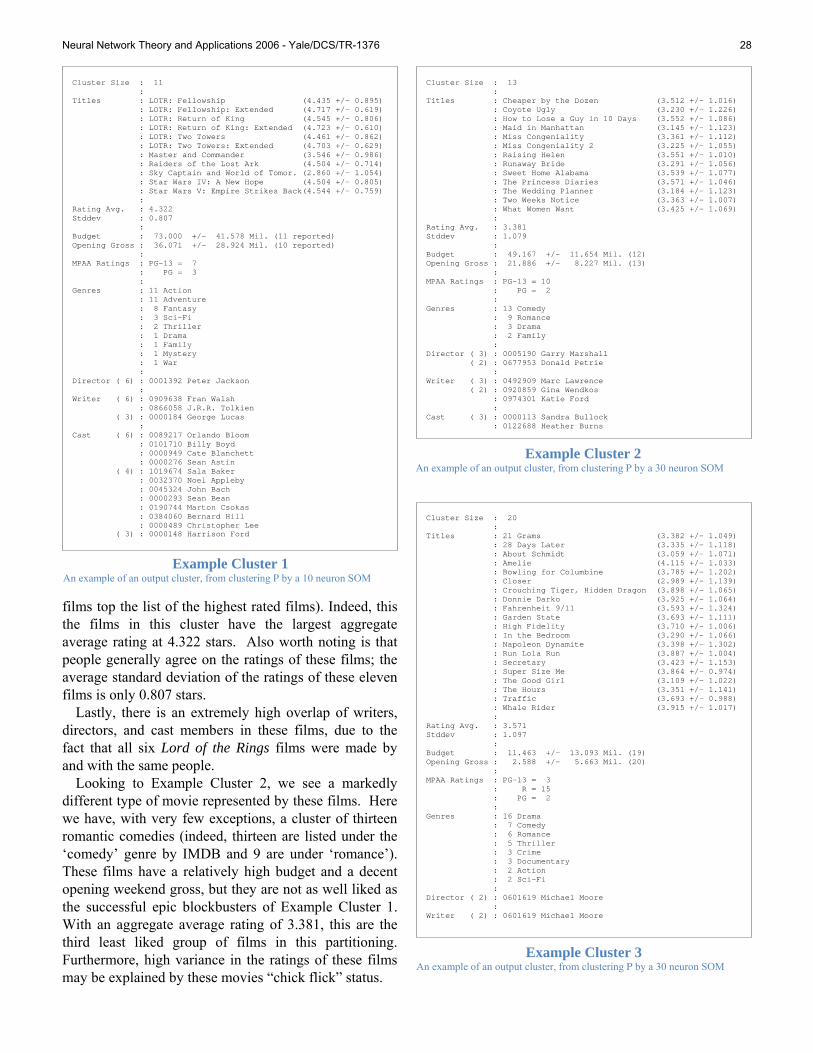
Neural Network Theory and Applications 2006 6
films top the list of the highest rated films). Indeed, this the films in this cluster have the largest aggregate average rating at 4.322 stars. Also worth noting is that people generally agree on the ratings of these films; the average standard deviation of the ratings of these eleven films is only 0.807 stars.
Lastly, there is an extremely high overlap of writers, directors, and cast members in these films, due to the fact that all six Lord of the Rings films were made by and with the same people.
Looking to Example Cluster 2, we see a markedly different type of movie represented by these films. Here we have, with very few exceptions, a cluster of thirteen romantic comedies (indeed, thirteen are listed under the ‘comedy’ genre by IMDB and 9 are under ‘romance’). These films have a relatively high budget and a decent opening weekend gross, but they are not as well liked as the successful epic blockbusters of Example Cluster 1. With an aggregate average rating of 3.381, this are the third least liked group of films in this partitioning. Furthermore, high variance in the ratings of these films may be explained by these movies “chick flick” status.
Cluster Size : 20 : Titles : 21 Grams (3.382 +/- 1.049) : 28 Days Later (3.335 +/- 1.118) : About Schmidt (3.059 +/- 1.071) : Amelie (4.115 +/- 1.033) : Bowling for Columbine (3.785 +/- 1.202) : Closer (2.989 +/- 1.139) : Crouching Tiger, Hidden Dragon (3.898 +/- 1.065) : Donnie Darko (3.925 +/- 1.064) : Fahrenheit 9/11 (3.593 +/- 1.324) : Garden State (3.693 +/- 1.111) : High Fidelity (3.710 +/- 1.006) : In the Bedroom (3.290 +/- 1.066) : Napoleon Dynamite (3.398 +/- 1.302) : Run Lola Run (3.887 +/- 1.004) : Secretary (3.423 +/- 1.153) : Super Size Me (3.864 +/- 0.974) : The Good Girl (3.109 +/- 1.022) : The Hours (3.351 +/- 1.141) : Traffic (3.693 +/- 0.988) : Whale Rider (3.915 +/- 1.017) : Rating Avg. : 3.571 Stddev : 1.097 : Budget : 11.463 +/- 13.093 Mil. (19) Opening Gross : 2.588 +/- 5.663 Mil. (20) : MPAA Ratings : PG-13 = 3 : R = 15 : PG = 2 : Genres : 16 Drama : 7 Comedy : 6 Romance : 5 Thriller : 3 Crime : 3 Documentary : 2 Action : 2 Sci-Fi : Director ( 2) : 0601619 Michael Moore : Writer ( 2) : 0601619 Michael Moore
Example Cluster 3 An example of an output cluster, from clustering R by a 30 neuron SOM
Example Cluster 1 An example of an output cluster, from clustering R by a 10 neuron SOM
Cluster Size : 11 : Titles : LOTR: Fellowship (4.435 +/- 0.895) : LOTR: Fellowship: Extended (4.717 +/- 0.619) : LOTR: Return of King (4.545 +/- 0.806) : LOTR: Return of King: Extended (4.723 +/- 0.610) : LOTR: Two Towers (4.461 +/- 0.862) : LOTR: Two Towers: Extended (4.703 +/- 0.629) : Master and Commander (3.546 +/- 0.986) : Raiders of the Lost Ark (4.504 +/- 0.714) : Sky Captain and World of Tomor. (2.860 +/- 1.054) : Star Wars IV: A New Hope (4.504 +/- 0.805) : Star Wars V: Empire Strikes Back(4.544 +/- 0.759) : Rating Avg. : 4.322 Stddev : 0.807 : Budget : 73.000 +/- 41.578 Mil. (11 reported) Opening Gross : 36.071 +/- 28.924 Mil. (10 reported) : MPAA Ratings : PG-13 = 7 : PG = 3 : Genres : 11 Action : 11 Adventure : 8 Fantasy : 3 Sci-Fi : 2 Thriller : 1 Drama : 1 Family : 1 Mystery : 1 War : Director ( 6) : 0001392 Peter Jackson : Writer ( 6) : 0909638 Fran Walsh : 0866058 J.R.R. Tolkien ( 3) : 0000184 George Lucas : Cast ( 6) : 0089217 Orlando Bloom : 0101710 Billy Boyd : 0000949 Cate Blanchett : 0000276 Sean Astin ( 4) : 1019674 Sala Baker : 0032370 Noel Appleby : 0045324 John Bach : 0000293 Sean Bean : 0190744 Marton Csokas : 0384060 Bernard Hill : 0000489 Christopher Lee ( 3) : 0000148 Harrison Ford
Cluster Size : 13 : Titles : Cheaper by the Dozen (3.512 +/- 1.016) : Coyote Ugly (3.230 +/- 1.226) : How to Lose a Guy in 10 Days (3.552 +/- 1.086) : Maid in Manhattan (3.145 +/- 1.123) : Miss Congeniality (3.361 +/- 1.112) : Miss Congeniality 2 (3.225 +/- 1.055) : Raising Helen (3.551 +/- 1.010) : Runaway Bride (3.291 +/- 1.056) : Sweet Home Alabama (3.539 +/- 1.077) : The Princess Diaries (3.571 +/- 1.046) : The Wedding Planner (3.184 +/- 1.123) : Two Weeks Notice (3.363 +/- 1.007) : What Women Want (3.425 +/- 1.069) : Rating Avg. : 3.381 Stddev : 1.079 : Budget : 49.167 +/- 11.654 Mil. (12) Opening Gross : 21.886 +/- 8.227 Mil. (13) : MPAA Ratings : PG-13 = 10 : PG = 2 : Genres : 13 Comedy : 9 Romance : 3 Drama : 2 Family : Director ( 3) : 0005190 Garry Marshall ( 2) : 0677953 Donald Petrie : Writer ( 3) : 0492909 Marc Lawrence ( 2) : 0920859 Gina Wendkos : 0974301 Katie Ford : Cast ( 3) : 0000113 Sandra Bullock : 0122688 Heather Burns
Example Cluster 2 An example of an output cluster, from clustering R by a 30 neuron SOM
Neural Network Theory and Applications 2006 - Yale/DCS/TR-1376 28

Neural Network Theory and Applications 2006 7
Example Cluster 3 poses a more difficult analysis. With respect to movie topics and subject matter, there is little that relates these films to each other. These films include documentaries and journeys in science fiction. Some are disheartening postmodern character studies, while others are uplifting romantic comedies. Given the knowledge of the difference in these films’ themes, has the partitioning scheme made an error?
Looking at this cluster from a different perspective reveals that there are ways to understand these movies with respect to each other. The average opening gross ranks in as the fourth lowest among all clusters. This indicates that these films were not initially well attended in theaters. This is generally true of these films—they are primarily movies with an indie following.
These are movies that have been very successful with one demographic group but no others. Michael Moore’s films, Bowling for Columbine and Fahrenheit 9/11, are generally watched by many who are politically liberal and by few conservatives. Similarly, Garden State and High Fidelity, which express the youth generation’s complaints about love and society, are generally watched by the 18-25 year old demographic.
There are four foreign films in this cluster (Amelie, Crouching Tiger, Hidden Dragon, Run Lola Run and Whale Rider), as well as three documentaries (Bowling for Columbine, Fahrenheit 9/11 and Super Size Me). This cluster has an alternative feel, with films that are not out to please any large audience.
VII. CONCLUSION The intangible quality of “indie-ness” that relates the
films in Example Cluster 3 demonstrates power in the SOM algorithm. By many standards, these films would not be grouped similarly, and yet this group shares many features that could be very meaningful in analyzing the films for a collaborative filtering system.
It is important to note, however, that SOM clustering technique is also very successful with films that are easier to classify. Films with clearly defined features are separated along these lines (e.g., epics and romantic comedies are divided into Example Clusters 1 and 2, respectively). Additionally, films in the same franchise made in similar ways with similar casts are extremely rarely split into different clusters.
Further quantitative validity of these clusterings could be garnered via the empirical results of a collaborative filtering scheme that utilizes these partitions, such as the content-boosted system proposed by Melville, Mooney and Nagaraan [4]. Qualitatively, however, these clusters are consistent with the author’s personal perspectives on
these films, and seem to be very meaningful with respect to the content data gathered from IMDB on these films.
It seems that the problems of scalability can be mitigated by using this algorithm. The data considered in the calculations that arrive at these clusterings are much fewer than the entire set of viewer-movie rating pairs. Indeed, one only needs a single relational number between any two films in order to create meaningful partitions of some product space. Only one step of pre-processing must be done before clustering the films via the SOM algorithm.
In addition to being extremely useful for collaborative filtering algorithms [4, 5, 6], this work can be altered to be applicable in many fields. The problem of clustering is important for all sorts of computational algorithms and models (from pattern classification and data mining to resource allocation and strategic management). In order to extend this algorithm to other problems, the only thing necessary is some feedback on the items that one wants to partition and a measure of how the similar the items are as a function of all of their feedback.
APPENDIX A Table 3 – Most Frequently Rated Films
Count Rating Title 233 3.361 Miss Congeniality 217 3.724 Independence Day 201 3.784 The Patriot 196 3.442 The Day After Tomorrow 194 4.154 Pirates of the Caribbean: Curse of the Black Pearl 193 3.905 Pretty Woman 182 4.300 Forrest Gump 181 4.307 The Green Mile 178 3.454 Con Air 178 3.412 Twister
Table 4 - Highest Rated Films Rating StdDev Title
4.723 0.372 LOTR: Return of King, Extended 4.717 0.383 LOTR: Fellowship of Ring, Extended 4.703 0.396 LOTR: The Two Towers, Extended 4.593 0.459 Shawshank Redemption, Special Ed. 4.545 0.649 LOTR: Return of the King 4.544 0.577 Star Wars, V: Empire Strikes Back 4.504 0.622 The Godfather 4.504 0.648 Star Wars, IV: A New Hope 4.504 0.509 Raiders of the Lost Ark 4.461 0.638 Star Wars, VI: Return of the Jedi
Table 5 - Lowest Rated Films Rating StdDev Title 2.798 1.003 The Stepford Wives 2.855 1.018 Hollow Man 2.856 1.196 Wild Wild West 2.860 1.110 Sky Captain and World of Tomorrow 2.901 1.639 Punch-Drunk Love 2.907 1.209 Legally Blonde 2 2.925 1.478 Anchorman 2.947 1.106 Once Upon a Time in Mexico 2.965 1.201 A.I. Artificial Intelligence 2.980 1.119 Daredevil
Neural Network Theory and Applications 2006 - Yale/DCS/TR-1376 29

Neural Network Theory and Applications 2006 8
Table 6 – Films with Highest Rating Variance Rating StdDev Title 3.593 1.752 Fahrenheit 9/11 3.398 1.697 Napoleon Dynamite 3.374 1.658 Moulin Rouge 3.280 1.656 The Royal Tenenbaums 2.901 1.639 Punch-Drunk Love 3.372 1.627 Lost in Translation 3.748 1.609 The Passion of the Christ 3.077 1.595 The Life Aquatic with Steve Zissou 3.230 1.503 Coyote Ugly 3.598 1.494 Sin City
Table 7 – Films with Lowest Rating Variance Rating StdDev Title 4.723 0.372 LOTR: Return of King, Extended 4.717 0.383 LOTR: Fellowship of Ring, Extended 4.703 0.396 LOTR: The Two Towers, Extended 4.593 0.459 The Shawshank Redemption Special Ed. 4.504 0.509 Raiders of the Lost Ark 4.544 0.577 Star Wars, V: Empire Strikes Back 4.416 0.603 Finding Nemo 4.458 0.611 Schindler's List 4.173 0.617 Stand by Me 4.504 0.622 The Godfather
Table 8 - Films with Highest Correlation (r'mn) Corr Rating Title
0.873 4.717 LOTR: Fellowship of Ring: Extended 4.703 LOTR: The Two Towers: Extended
0.850 4.723 LOTR: Return of King: Extended 4.703 LOTR: The Two Towers: Extended
0.839 4.723 LOTR: Return of King: Extended 4.717 LOTR: Fellowship of Ring: Extended
0.814 4.435 LOTR: The Fellowship of the Ring 4.461 LOTR: The Two Towers
0.801 4.092 Harry Potter and the Sorcerer's Stone 4.045 Harry Potter and the Chamber of Secrets
0.785 4.545 LOTR: The Return of the King 4.461 LOTR: The Two Towers
0.764 3.814 Lethal Weapon 3 3.877 Lethal Weapon 2
0.761 4.545 LOTR: The Return of the King 4.435 LOTR: The Fellowship of the Ring
0.757 3.874 Kill Bill: Vol. 2 3.759 Kill Bill: Vol. 1
0.754 3.604 Star Wars, I: The Phantom Menace 3.550 Star Wars, II: Attack of the Clones
Table 9 - Films with Lowest Correlation (r'mn) Corr Rating Title
-0.267 3.280 The Royal Tenenbaums 3.398 Pearl Harbor
-0.258 2.901 Punch-Drunk Love 3.398 Pearl Harbor
-0.253 3.372 Lost in Translation 3.398 Pearl Harbor
-0.253 3.725 Annie Hall 3.583 Armageddon
-0.249 3.352 Adaptation 3.398 Pearl Harbor
-0.241 3.372 Lost in Translation 3.583 Armageddon
-0.239 3.725 Annie Hall 3.398 Pearl Harbor
-0.237 3.280 The Royal Tenenbaums 3.583 Armageddon
-0.235 2.901 Punch-Drunk Love 3.640 Double Jeopardy
-0.234 2.901 Punch-Drunk Love 3.583 Armageddon
Table 10 - Films of Highest Distance (d'mn) Distance Rating Title
1.000 4.094 Pulp Fiction 3.361 Miss Congeniality
0.964 4.300 Forrest Gump 3.361 Miss Congeniality
0.952 3.280 The Royal Tenenbaums 3.361 Miss Congeniality
0.951 3.963 American Beauty 3.361 Miss Congeniality
0.948 3.280 The Royal Tenenbaums 4.300 Forrest Gump
0.944 4.593 The Shawshank Redemption: Special Ed. 3.361 Miss Congeniality
0.937 4.461 Lord of the Rings: Two Towers 3.361 Miss Congeniality
0.936 4.307 The Green Mile 3.361 Miss Congeniality
0.935 4.435 Lord of the Rings: Fellowship of the Ring 3.361 Miss Congeniality
0.933 3.372 Lost in Translation 4.094 Forrest Gump
Table 11 - Films of Lowest Distance (d'mn) Distance Rating Title
0.124 4.717 LOTR: Fellowship of the Ring: Extended 4.703 LOTR: Two Towers: Extended
0.131 4.723 LOTR: Return of the King: Extended 4.703 LOTR: Two Towers: Extended
0.134 4.723 LOTR: Return of the King: Extended 4.717 LOTR: Fellowship of the Ring: Extended
0.170 4.723 LOTR: Return of the King: Extended 4.545 LOTR: Return of the King
0.187 3.609 Shall We Dance? 3.790 In the Line of Fire
0.188 4.717 LOTR: Fellowship of the Ring: Extended 4.545 LOTR: Return of the King
0.188 4.703 LOTR: Two Towers: Extended 4.545 LOTR: Return of the King
0.190 3.766 Rules of Engagement 3.609 Shall We Dance?
0.190 4.241 Rear Window 4.071 Coach Carter
0.191 4.703 LOTR: Two Towers: Extended 4.461 LOTR: Two Towers
ACKNOWLEDGMENT A. Pariser would like to thank the Yale University Computer Science
department for providing a venue to study this data, as well as Frederick Shic for helping focus the project. Thanks are also due to Daniel Spielman, who provided the author insight into ways to analyze clusters.
REFERENCES [1] S. Harnad, “Cognition is Categorization”, in Cohen, Henri and Lefebvre,
Claire, Eds. Handbook of Categorization, Elsevier, 2005. [2] S. Haykin, Neural Networks: A Comprehensive Foundation (Upper
Saddle River, NJ: Prentice-Hall, 1999). [3] E. Kreyszig, Advanced Engineering Mathematics, 8th Ed. (Hoboken, NJ:
John Wiley & Sons, Inc., 1999). [4] P. Melville, R.J. Mooney and R. Nagarajan, “Content-Boosted
Collaborative Filtering for Improved Recommendations” in Proceedings of the Eighteenth National Conference on Artificial Intelligence (AAAI, 2002), pp. 187-192, Edmonton, Canada, July 2002.
[5] M. O’Connor and J. Herlocker, “Clustering Items for Collaborative Filtering” in Proceedings of the ACM SIGIR Workshop on Recommender Systems, Berkeley, CA, 1999.
[6] G.R. Xue, C. Lin, Q. Yang, et. Al., “Scalable Collaborative Filtering Using Cluster-based Smoothing” in Proceedings of the 2005 ACM SIGIR Conference, Salvador, Brazil, 2005, pp. 114-121
Neural Network Theory and Applications 2006 - Yale/DCS/TR-1376 30
Abstract—The conventional face recognition system consists of two parts: training and classification. The training part normally includes principle component analysis to reduce the dimensionality of images. In classification, a query image is projected to the reduced dimension and then compared with training images. Both training and classification could be done using neural networks’ techniques. Specifically, PCA in the training phase could be done by neural network with Hebbian learning and the classification could also be done using a feed forward net. This paper compares the conventional techniques of face recognition with the techniques from neural networks.
Index Terms—face recognition, eigenvalue, eigenvector, eigenface, principle component analysis, singular value decomposition, neural network, hebbian learning, feed forward net, backpropogation
I. INTRODUCTION
ACE recognition has become a central technology for identity verification. Commercial systems are already
widely used in access control and proactive surveillance applications all over the world.
Face recognition is not an easy task because of two major obstacles. Lighting conditions could significantly distort the content of the image. Makeup, hairdo and outfit could significantly change an individual’s appearance. A pair of images of the same individual may look dramatically different. Such difficulties can make recognition extremely challenging. Moreover, difference in facial expressions also complicates the recognition problem. We shall, for simplicity, assume the lighting conditions are fairly constant. A good and robust face recognition system should work on faces with slight facial expressions. For convenience and simplicity, we only consider vertically oriented grey scale images.
Face recognition begins with a collection of labeled images. The label identifies the individual in the image. These labeled images, also called training images, are the bases for
developing the recognition system. Typically, images are of size 100 pixels by 100 pixels, or more. For grey scale images, each pixel could take on any value between 0 and 255. Therefore, ten thousand dimensions of data need to be considered. Such high dimensionality of image data contributes to complexity of the problem. Since a large number of pixels could change their values due to a slight change in lighting and facial expression, recognition by comparing corresponding pixels in a pair of images is very inefficient and non-robust.
A more advanced face recognition system consists of two phases: training and classification. The first phase consists of training a system on a set of labeled images. The primary task of training is to reduce the dimensionality of the training images. Training is an offline process and it allows the classification phase, an online process, to perform comparisons among images in the reduced dimension.
To achieve the reduction of dimensions, the standard face recognition system uses principle component analysis (PCA). As well known, PCA presents the data in a way that maximizes the variance within the data. A nearest neighbor classifier could then be used to compare a pair of images in the reduced dimension by computing the Euclidean distance between them. The winner of this classification protocol is the labeled image that has the shortest distance from the target image in the reduced dimension.
Both the training and classification phases of the algorithm could be performed using neural networks. A neural network using Hebbian learning also produces the principle components. A feed forward net could be used in place of the nearest neighbor classifier in the classification phase.
Section II will present two different techniques for the training phase, namely the eigenface technique and the Hebbian learning neural network. Both are used to find the principle components. The classification could use either a nearest neighbor classifier or a feed forward net. These will be introduced in Section III. Since we have two options for training and two options for classification, there are total of four ways to construct the face recognition algorithm. In section IV, the performance of each of the four algorithms are presented and compared. The advantages and disadvantages of each option are discussed. Conclusion will be in section V.
Face Recognition A Comparative Study
Yan Sui
Computer Science Department, Yale University
F
Neural Network Theory and Applications 2006 - Yale/DCS/TR-1376 31

II. TRAINING
A. Eigenface
Principle component analysis, originated as a statistical
analysis technique, identifies a way to represent high dimensional data in lower dimensions. The representation of the training images in lower dimensions is called the eigenfaces. See figure 3b). Eigenfaces have two important properties. The dimensions, or eigenfaces, are orthogonal to one another. A good estimate of the original data can be reconstructed by simply sum up the eigenfaces.
An outline of an algorithm to find eigenfaces from images is listed below:
1. For each training image i = 1 … m, place its pixels into
a column vector x i. m is the number of images.
2. Compute the mean face of the training images: µ
µ = 1m
x i
i = 1
m
∑
Figure 1 shows an example of the mean face. 3. Compute the covariance matrix: ∑
Σ = 1m −1
(x i − µ)(x i − µ)T
i=1
m
∑
4. Compute the eigenvalues and eigenvectors of the covariance matrix ∑
5. Choose the first K eigenvectors of ∑ that correspond to the largest K eigenvalues
6. Project the training images onto the principle component subspace of dimension K
Note in step 3, the covariance matrix has high dimensions, p
by p, where p is the number of pixels in each image. It is memory intensive to compute such covariance matrix. Fortunately, eigenvectors can be computed without first computing the covariance matrix ∑, by using singular value decomposition (SVD).
If we combine the m column vectors into a matrix A
A = x1 x2 L
xm[ ]
and subtract the mean face µ from each training image A = A − µ
therefore, Σ = AAT (ignore the scalar 1
m −1)
According to SVD, any m by n matrix A may be factored as
the following:
A = U S V T where U is of size m by m, S is of size m by n, and V is of size n by n. Also, the columns of U are the eigenvectors of
AAT . They are conveniently sorted by their corresponding eigenvalues, in descending order. The columns of V are the
eigenvectors of AT A. The diagonal of S are the singular
values, or the square roots of the eigenvalues of AAT , in descending order.
Therefore, the first K columns of matrix U are the same as the eigenvectors of the covariance matrix ∑ that correspond to the K highest eigenvalues.
B. Neural Network using Generalized Hebbian Algorithm
Besides eigenface, principle components can also be
computed using neural network with Hebbian learning. A visualization of the neural network to compute the first K principle components is shown in figure 2.
Here, there are m input nodes and k output nodes. m is the
number of pixels in the images and k is the number of principle components to be computed. There is a weight value associated with each edge in the figure. The weights can be written in matrix form w . The following functions are used to update the weight matrix w .
Fig 2. Neural Network for Hebbian Learning Here m is number of pixels in each image
Figure 1. an example of mean face
Neural Network Theory and Applications 2006 - Yale/DCS/TR-1376 32
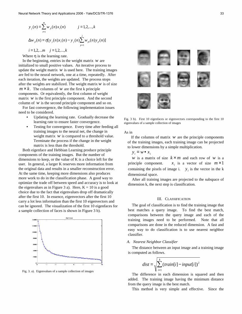
Where η is the learning rate. In the beginning, entries in the weight matrix w are
initialized to small positive values. An iterative process to update the weight matrix w is used here. The training images are fed to the neural network, one at a time, repeatedly. After each iteration, the weights are updated. The process stops after the weights are stabilized. The weight matrixw is of size m × k . The columns of w are the first k principle components. Or equivalently, the first column of weight matrix w is the first principle component. And the second column of w is the second principle component and so on.
For fast convergence, the following implementation issues need to be considered.
• Updating the learning rate. Gradually decrease the learning rate to ensure faster convergence.
• Testing for convergence. Every time after feeding all training images to the neural net, the change in weight matrix w is compared to a threshold value. Terminate the process if the change in the weight matrix is less than the threshold.
Both eigenface and Hebbian Learning produce principle components of the training images. But the number of dimensions to keep, or the value of K is a choice left for the user. In general, a larger K reserves more information from the original data and results in a smaller reconstruction error. At the same time, keeping more dimensions also produces more work to do in the classification phase. A good way to optimize the trade off between speed and accuracy is to look at the eigenvalues as in Figure 3 a). Here, K = 10 is a good choice due to the fact that eigenvalues drop off dramatically after the first 10. In essence, eigenvectors after the first 10 carry a lot less information than the first 10 eigenvectors and can be ignored. The visualization of the first 10 eigenfaces for a sample collection of faces is shown in Figure 3 b).
Fig. 3 b). First 10 eigenfaces or eigenvectors corresponding to the first 10 eigenvalues of a sample collection of images
As in
If the columns of matrix w are the principle components of the training images, each training image can be projected to lower dimensions by a simple multiplication.
y i = w • x i
w is a matrix of size k × m and each row of w is a principle component. x i is a vector of size m ×1
containing the pixels of image i. y i is the vector in the k
dimensional space. After all training images are projected to the subspace of
dimension k, the next step is classification.
III. CLASSIFICATION
The goal of classification is to find the training image that best matches a query image. To find the best match, comparisons between the query image and each of the training images need to be performed. Note that all comparisons are done in the reduced dimension. A fast and easy way to do classification is to use nearest neighbor classifier.
A. Nearest Neighbor Classifier
The distance between an input image and a training image is computed as follows.
The difference in each dimension is squared and then added. The training image having the minimum distance from the query image is the best match.
This method is very simple and effective. Since the
y j (n) = w ji(n)x i(n)i=1
m
∑ j =1,2,...,k
∆w ji(n) = η[y j (n)x i(n) − y j (n) w pi(n)y p (n)p=1
j
∑ ]
i =1,2,...m j =1,2,...,k
dist = (train[i] − input[i])2
i=1
k
∑dist = (train[i] − input[i])2
i=1
k
∑
Fig. 3. a). Eigenvalues of a sample collection of images
Neural Network Theory and Applications 2006 - Yale/DCS/TR-1376 33
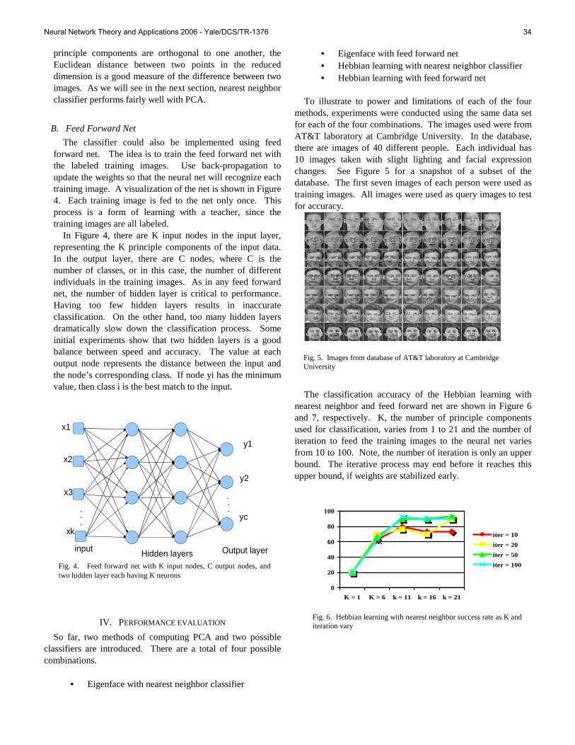
principle components are orthogonal to one another, the Euclidean distance between two points in the reduced dimension is a good measure of the difference between two images. As we will see in the next section, nearest neighbor classifier performs fairly well with PCA.
B. Feed Forward Net
The classifier could also be implemented using feed forward net. The idea is to train the feed forward net with the labeled training images. Use back-propagation to update the weights so that the neural net will recognize each training image. A visualization of the net is shown in Figure 4. Each training image is fed to the net only once. This process is a form of learning with a teacher, since the training images are all labeled.
In Figure 4, there are K input nodes in the input layer, representing the K principle components of the input data. In the output layer, there are C nodes, where C is the number of classes, or in this case, the number of different individuals in the training images. As in any feed forward net, the number of hidden layer is critical to performance. Having too few hidden layers results in inaccurate classification. On the other hand, too many hidden layers dramatically slow down the classification process. Some initial experiments show that two hidden layers is a good balance between speed and accuracy. The value at each output node represents the distance between the input and the node’s corresponding class. If node yi has the minimum value, then class i is the best match to the input.
IV. PERFORMANCE EVALUATION
So far, two methods of computing PCA and two possible classifiers are introduced. There are a total of four possible combinations.
• Eigenface with nearest neighbor classifier
• Eigenface with feed forward net • Hebbian learning with nearest neighbor classifier • Hebbian learning with feed forward net
To illustrate to power and limitations of each of the four
methods, experiments were conducted using the same data set for each of the four combinations. The images used were from AT&T laboratory at Cambridge University. In the database, there are images of 40 different people. Each individual has 10 images taken with slight lighting and facial expression changes. See Figure 5 for a snapshot of a subset of the database. The first seven images of each person were used as training images. All images were used as query images to test for accuracy.
The classification accuracy of the Hebbian learning with
nearest neighbor and feed forward net are shown in Figure 6 and 7, respectively. K, the number of principle components used for classification, varies from 1 to 21 and the number of iteration to feed the training images to the neural net varies from 10 to 100. Note, the number of iteration is only an upper bound. The iterative process may end before it reaches this upper bound, if weights are stabilized early.
x1
x2
x3
xk
y1
y2
yc...
...
Hidden layers Output layerinput
Fig. 4. Feed forward net with K input nodes, C output nodes, and two hidden layer each having K neurons
0
20
40
60
80
100
K = 1 K = 6 k = 11 k = 16 k = 21
iter = 10
iter = 20
iter = 50
iter = 100
Fig. 6. Hebbian learning with nearest neighbor success rate as K and iteration vary
Fig. 5. Images from database of AT&T laboratory at Cambridge University
Neural Network Theory and Applications 2006 - Yale/DCS/TR-1376 34

For Hebbian learning with nearest neighbor classifier,
accuracy gets better as the value of K and the number of iterations increases. The accuracy of Hebbian learning with feed forward net is relatively consistent as shown in figure 7. Notice that the accuracy in figure 7 is greater than 70% even when K = 1. This is due to feed forward net’s ability to correctly recognize the training images.
The classification accuracy of eigenface with both nearest
neighbor and feed forward net is given in figure 8. We can plot the four combinations on the same graph to
better visualize of the comparison, as shown in Figure 9.
Several interesting points to note:
• For the training phase, eigenface produces slightly higher accuracy. This is expected because hebbian learning is an iterative process that estimates the principle components. Errors in principle components need to be tolerated when using hebbian learning. Eigenface, on the other hand, finds the optimal solution in one shot.
• For classification, nearest neighbor does a slightly better job than feed forward net, when K >= 11. Feed forward net does a better job than nearest neighbor, when K < 11. This is due to the fact that nearest neighbor needs good results of PCA to work well. When K is large, more information about the data is captured in the principle components. Thus nearest neighbor performs better. Conversely, feed forward net does not require as much information to recognize the training images.
V. CONCLUSION
Face recognition, when assuming good lighting condition, is
a well-researched problem. The simple and effective way to do face recognition is to use eigenface with nearest neighbor classifier. As shown in this paper, it works reasonably well. While face recognition can also be implemented using neural network techniques, it is not commonly used in this field. The major problem with neural network in face recognition is not the accuracy but speed. For both training and classification, neural network runs a lot slower than the simple eigenvector calculation. The iterative process of neural network limits its applicability to face recognition problems. In addition, as we discussed, when using neural network, there are a number of parameters that need to be carefully initialized and updated before and during the iterative process. This also makes the use of neural network more complicated and less desirable than eigenface.
Feed forward net recognizes the training images very accurately with little help from the training phase. It works exceptionally well in recognizing images it has seen before. For applications whose query images are a subset of its training images, feed forward net could be the leading candidate for classification.
Currently in face recognition, the query image needs to be compared to each and every training image in the training set during classification. If there are a large number of training images, the large number of comparisons will significantly reduce the speed of recognition system. Instead, the query image should only need to be compared with each class in the training set. For future studies in face recognition, instead of features describing each individual image, features describing
65
70
75
80
85
90
K = 1 K = 6 K = 11 K = 16 K = 21
iter = 10
iter = 20
iter = 50
iter = 100
Fig. 7. Hebbian learning with feed forward net success rate as K and iteration vary. Note that in the case of feed forward net, the result is fairly consistent with different number of principle components.
0
20
40
60
80
100
120
K = 1 K = 6 K = 11 K = 16 K = 21
NearestNeighbor
FeedforwardNet
Fig. 8. Eigenface with nearest neighbor and feed forward net varying the value of K
0
20
40
60
80
100
120
k = 1 k = 5 k = 11 k = 16 k = 21
Hebbian, FFNet
Eigen, Near Neighbor
eigen, FFNet
Hebbian, Near Neighbor
Fig. 9. Accuracy of all four combinations as K increases. Note: Accuracy for Hebbian Learning is sampled at iteration = 50
Neural Network Theory and Applications 2006 - Yale/DCS/TR-1376 35
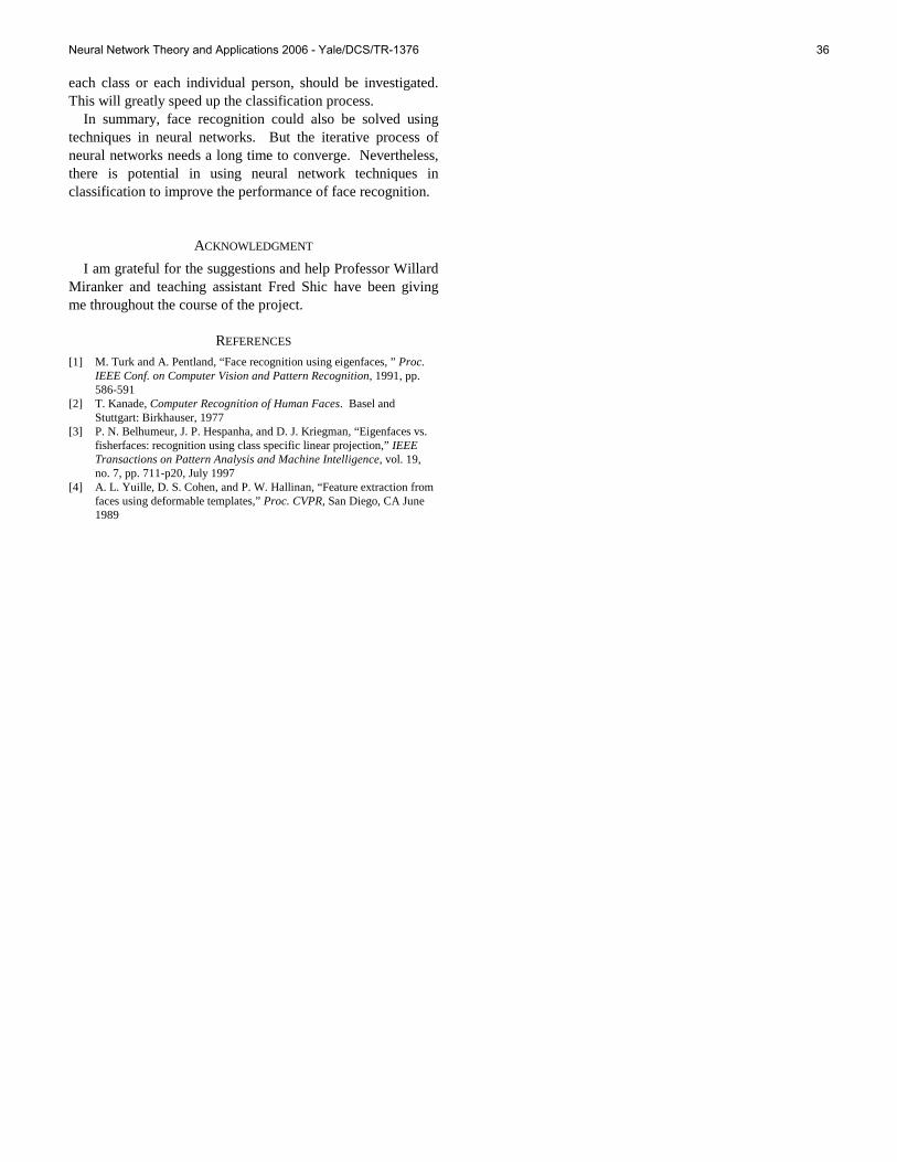
each class or each individual person, should be investigated. This will greatly speed up the classification process.
In summary, face recognition could also be solved using techniques in neural networks. But the iterative process of neural networks needs a long time to converge. Nevertheless, there is potential in using neural network techniques in classification to improve the performance of face recognition.
ACKNOWLEDGMENT
I am grateful for the suggestions and help Professor Willard Miranker and teaching assistant Fred Shic have been giving me throughout the course of the project.
REFERENCES
[1] M. Turk and A. Pentland, “Face recognition using eigenfaces, ” Proc. IEEE Conf. on Computer Vision and Pattern Recognition, 1991, pp. 586-591
[2] T. Kanade, Computer Recognition of Human Faces. Basel and Stuttgart: Birkhauser, 1977
[3] P. N. Belhumeur, J. P. Hespanha, and D. J. Kriegman, “Eigenfaces vs. fisherfaces: recognition using class specific linear projection,” IEEE Transactions on Pattern Analysis and Machine Intelligence, vol. 19, no. 7, pp. 711-p20, July 1997
[4] A. L. Yuille, D. S. Cohen, and P. W. Hallinan, “Feature extraction from faces using deformable templates,” Proc. CVPR, San Diego, CA June 1989
Neural Network Theory and Applications 2006 - Yale/DCS/TR-1376 36
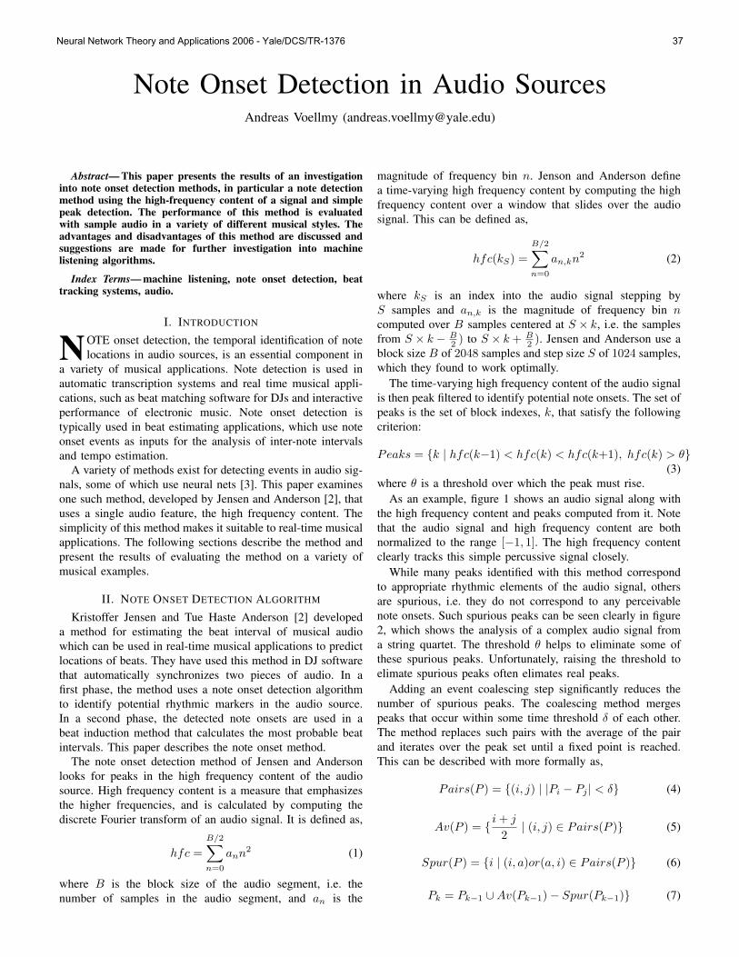
NEURAL NETWORK THEORY AND APPLICATIONS 2006 1
Note Onset Detection in Audio SourcesAndreas Voellmy ([email protected])
Abstract— This paper presents the results of an investigationinto note onset detection methods, in particular a note detectionmethod using the high-frequency content of a signal and simplepeak detection. The performance of this method is evaluatedwith sample audio in a variety of different musical styles. Theadvantages and disadvantages of this method are discussed andsuggestions are made for further investigation into machinelistening algorithms.
Index Terms— machine listening, note onset detection, beattracking systems, audio.
I. INTRODUCTION
NOTE onset detection, the temporal identification of notelocations in audio sources, is an essential component in
a variety of musical applications. Note detection is used inautomatic transcription systems and real time musical appli-cations, such as beat matching software for DJs and interactiveperformance of electronic music. Note onset detection istypically used in beat estimating applications, which use noteonset events as inputs for the analysis of inter-note intervalsand tempo estimation.
A variety of methods exist for detecting events in audio sig-nals, some of which use neural nets [3]. This paper examinesone such method, developed by Jensen and Anderson [2], thatuses a single audio feature, the high frequency content. Thesimplicity of this method makes it suitable to real-time musicalapplications. The following sections describe the method andpresent the results of evaluating the method on a variety ofmusical examples.
II. NOTE ONSET DETECTION ALGORITHM
Kristoffer Jensen and Tue Haste Anderson [2] developeda method for estimating the beat interval of musical audiowhich can be used in real-time musical applications to predictlocations of beats. They have used this method in DJ softwarethat automatically synchronizes two pieces of audio. In afirst phase, the method uses a note onset detection algorithmto identify potential rhythmic markers in the audio source.In a second phase, the detected note onsets are used in abeat induction method that calculates the most probable beatintervals. This paper describes the note onset method.
The note onset detection method of Jensen and Andersonlooks for peaks in the high frequency content of the audiosource. High frequency content is a measure that emphasizesthe higher frequencies, and is calculated by computing thediscrete Fourier transform of an audio signal. It is defined as,
hfc =B/2∑n=0
ann2 (1)
where B is the block size of the audio segment, i.e. thenumber of samples in the audio segment, and an is the
magnitude of frequency bin n. Jenson and Anderson definea time-varying high frequency content by computing the highfrequency content over a window that slides over the audiosignal. This can be defined as,
hfc(kS) =B/2∑n=0
an,kn2 (2)
where kS is an index into the audio signal stepping byS samples and an,k is the magnitude of frequency bin ncomputed over B samples centered at S × k, i.e. the samplesfrom S × k − B
2 ) to S × k + B2 ). Jensen and Anderson use a
block size B of 2048 samples and step size S of 1024 samples,which they found to work optimally.
The time-varying high frequency content of the audio signalis then peak filtered to identify potential note onsets. The set ofpeaks is the set of block indexes, k, that satisfy the followingcriterion:
Peaks = {k | hfc(k−1) < hfc(k) < hfc(k+1), hfc(k) > θ}(3)
where θ is a threshold over which the peak must rise.As an example, figure 1 shows an audio signal along with
the high frequency content and peaks computed from it. Notethat the audio signal and high frequency content are bothnormalized to the range [−1, 1]. The high frequency contentclearly tracks this simple percussive signal closely.
While many peaks identified with this method correspondto appropriate rhythmic elements of the audio signal, othersare spurious, i.e. they do not correspond to any perceivablenote onsets. Such spurious peaks can be seen clearly in figure2, which shows the analysis of a complex audio signal froma string quartet. The threshold θ helps to eliminate some ofthese spurious peaks. Unfortunately, raising the threshold toelimate spurious peaks often elimates real peaks.
Adding an event coalescing step significantly reduces thenumber of spurious peaks. The coalescing method mergespeaks that occur within some time threshold δ of each other.The method replaces such pairs with the average of the pairand iterates over the peak set until a fixed point is reached.This can be described with more formally as,
Pairs(P ) = {(i, j) | |Pi − Pj | < δ} (4)
Av(P ) = { i + j
2| (i, j) ∈ Pairs(P )} (5)
Spur(P ) = {i | (i, a)or(a, i) ∈ Pairs(P )} (6)
Pk = Pk−1 ∪Av(Pk−1)− Spur(Pk−1)} (7)
Neural Network Theory and Applications 2006 - Yale/DCS/TR-1376 37
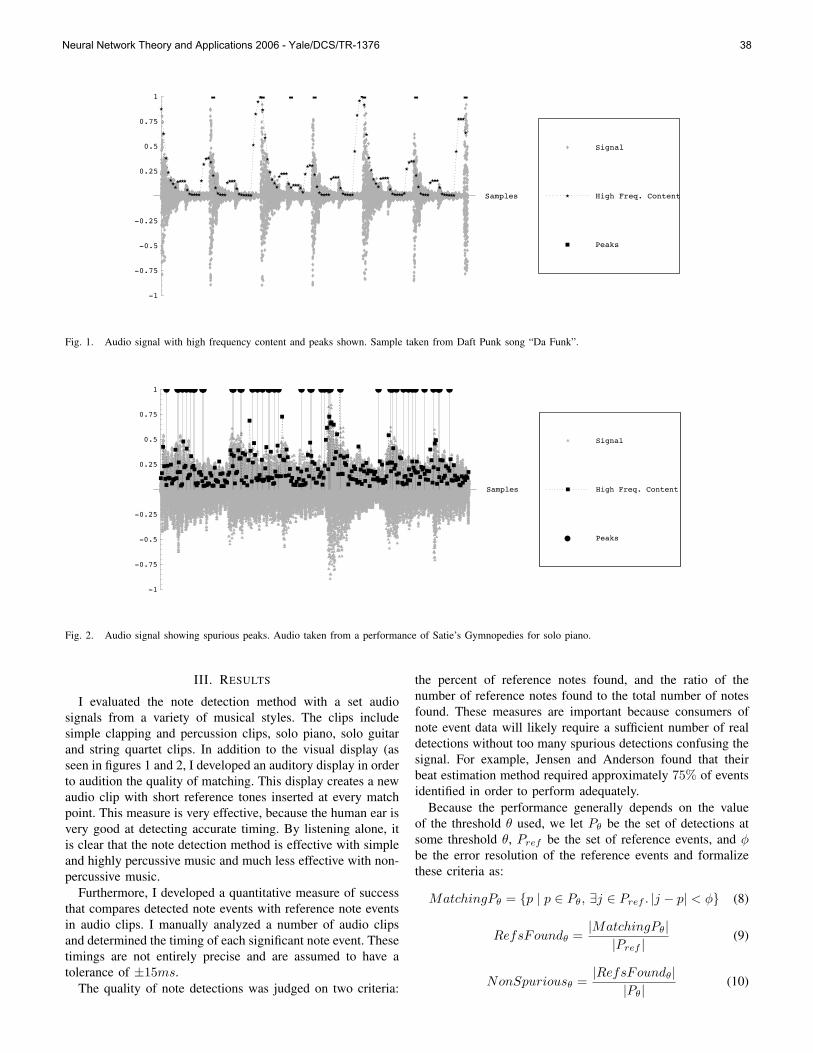
Samples
-1
-0.75
-0.5
-0.25
0.25
0.5
0.75
1
Peaks
High Freq. Content
Signal
Fig. 1. Audio signal with high frequency content and peaks shown. Sample taken from Daft Punk song “Da Funk”.
Samples
-1
-0.75
-0.5
-0.25
0.25
0.5
0.75
1
Peaks
High Freq. Content
Signal
Fig. 2. Audio signal showing spurious peaks. Audio taken from a performance of Satie’s Gymnopedies for solo piano.
III. RESULTS
I evaluated the note detection method with a set audiosignals from a variety of musical styles. The clips includesimple clapping and percussion clips, solo piano, solo guitarand string quartet clips. In addition to the visual display (asseen in figures 1 and 2, I developed an auditory display in orderto audition the quality of matching. This display creates a newaudio clip with short reference tones inserted at every matchpoint. This measure is very effective, because the human ear isvery good at detecting accurate timing. By listening alone, itis clear that the note detection method is effective with simpleand highly percussive music and much less effective with non-percussive music.
Furthermore, I developed a quantitative measure of successthat compares detected note events with reference note eventsin audio clips. I manually analyzed a number of audio clipsand determined the timing of each significant note event. Thesetimings are not entirely precise and are assumed to have atolerance of ±15ms.
The quality of note detections was judged on two criteria:
the percent of reference notes found, and the ratio of thenumber of reference notes found to the total number of notesfound. These measures are important because consumers ofnote event data will likely require a sufficient number of realdetections without too many spurious detections confusing thesignal. For example, Jensen and Anderson found that theirbeat estimation method required approximately 75% of eventsidentified in order to perform adequately.
Because the performance generally depends on the valueof the threshold θ used, we let Pθ be the set of detections atsome threshold θ, Pref be the set of reference events, and φbe the error resolution of the reference events and formalizethese criteria as:
MatchingPθ = {p | p ∈ Pθ, ∃j ∈ Pref . |j − p| < φ} (8)
RefsFoundθ =|MatchingPθ|
|Pref |(9)
NonSpuriousθ =|RefsFoundθ|
|Pθ|(10)
Neural Network Theory and Applications 2006 - Yale/DCS/TR-1376 38
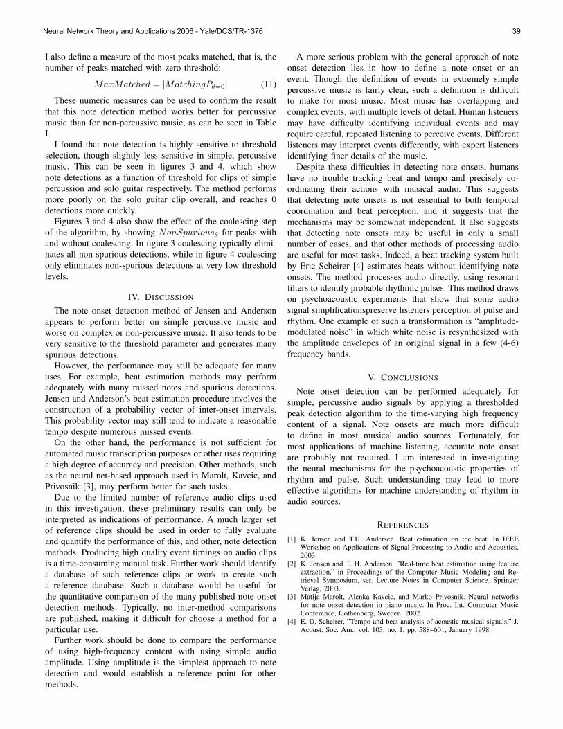
NEURAL NETWORK THEORY AND APPLICATIONS 2006 3
I also define a measure of the most peaks matched, that is, thenumber of peaks matched with zero threshold:
MaxMatched = |MatchingPθ=0| (11)
These numeric measures can be used to confirm the resultthat this note detection method works better for percussivemusic than for non-percussive music, as can be seen in TableI.
I found that note detection is highly sensitive to thresholdselection, though slightly less sensitive in simple, percussivemusic. This can be seen in figures 3 and 4, which shownote detections as a function of threshold for clips of simplepercussion and solo guitar respectively. The method performsmore poorly on the solo guitar clip overall, and reaches 0detections more quickly.
Figures 3 and 4 also show the effect of the coalescing stepof the algorithm, by showing NonSpuriousθ for peaks withand without coalescing. In figure 3 coalescing typically elimi-nates all non-spurious detections, while in figure 4 coalescingonly eliminates non-spurious detections at very low thresholdlevels.
IV. DISCUSSION
The note onset detection method of Jensen and Andersonappears to perform better on simple percussive music andworse on complex or non-percussive music. It also tends to bevery sensitive to the threshold parameter and generates manyspurious detections.
However, the performance may still be adequate for manyuses. For example, beat estimation methods may performadequately with many missed notes and spurious detections.Jensen and Anderson’s beat estimation procedure involves theconstruction of a probability vector of inter-onset intervals.This probability vector may still tend to indicate a reasonabletempo despite numerous missed events.
On the other hand, the performance is not sufficient forautomated music transcription purposes or other uses requiringa high degree of accuracy and precision. Other methods, suchas the neural net-based approach used in Marolt, Kavcic, andPrivosnik [3], may perform better for such tasks.
Due to the limited number of reference audio clips usedin this investigation, these preliminary results can only beinterpreted as indications of performance. A much larger setof reference clips should be used in order to fully evaluateand quantify the performance of this, and other, note detectionmethods. Producing high quality event timings on audio clipsis a time-consuming manual task. Further work should identifya database of such reference clips or work to create sucha reference database. Such a database would be useful forthe quantitative comparison of the many published note onsetdetection methods. Typically, no inter-method comparisonsare published, making it difficult for choose a method for aparticular use.
Further work should be done to compare the performanceof using high-frequency content with using simple audioamplitude. Using amplitude is the simplest approach to notedetection and would establish a reference point for othermethods.
A more serious problem with the general approach of noteonset detection lies in how to define a note onset or anevent. Though the definition of events in extremely simplepercussive music is fairly clear, such a definition is difficultto make for most music. Most music has overlapping andcomplex events, with multiple levels of detail. Human listenersmay have difficulty identifying individual events and mayrequire careful, repeated listening to perceive events. Differentlisteners may interpret events differently, with expert listenersidentifying finer details of the music.
Despite these difficulties in detecting note onsets, humanshave no trouble tracking beat and tempo and precisely co-ordinating their actions with musical audio. This suggeststhat detecting note onsets is not essential to both temporalcoordination and beat perception, and it suggests that themechanisms may be somewhat independent. It also suggeststhat detecting note onsets may be useful in only a smallnumber of cases, and that other methods of processing audioare useful for most tasks. Indeed, a beat tracking system builtby Eric Scheirer [4] estimates beats without identifying noteonsets. The method processes audio directly, using resonantfilters to identify probable rhythmic pulses. This method drawson psychoacoustic experiments that show that some audiosignal simplificationspreserve listeners perception of pulse andrhythm. One example of such a transformation is “amplitude-modulated noise” in which white noise is resynthesized withthe amplitude envelopes of an original signal in a few (4-6)frequency bands.
V. CONCLUSIONS
Note onset detection can be performed adequately forsimple, percussive audio signals by applying a thresholdedpeak detection algorithm to the time-varying high frequencycontent of a signal. Note onsets are much more difficultto define in most musical audio sources. Fortunately, formost applications of machine listening, accurate note onsetare probably not required. I am interested in investigatingthe neural mechanisms for the psychoacoustic properties ofrhythm and pulse. Such understanding may lead to moreeffective algorithms for machine understanding of rhythm inaudio sources.
REFERENCES
[1] K. Jensen and T.H. Andersen. Beat estimation on the beat. In IEEEWorkshop on Applications of Signal Processing to Audio and Acoustics,2003.
[2] K. Jensen and T. H. Andersen, ”Real-time beat estimation using featureextraction,” in Proceedings of the Computer Music Modeling and Re-trieval Symposium, ser. Lecture Notes in Computer Science. SpringerVerlag, 2003.
[3] Matija Marolt, Alenka Kavcic, and Marko Privosnik. Neural networksfor note onset detection in piano music. In Proc. Int. Computer MusicConference, Gothenberg, Sweden, 2002.
[4] E. D. Scheirer, ”Tempo and beat analysis of acoustic musical signals,” J.Acoust. Soc. Am., vol. 103, no. 1, pp. 588–601, January 1998.
Neural Network Theory and Applications 2006 - Yale/DCS/TR-1376 39

NEURAL NETWORK THEORY AND APPLICATIONS 2006 4
TABLE IEVENTS MATCHED BY REFERENCE CLIP
Clip Description MaxMatchedClap3.aif monophonic clap 1.0
DaFunk-Short-1.aif simple percussive 1.0DaFunkFill-Short-1.aif simple percussive, high-pass filtered 0.67
Starobin-Short-1.aif solo guitar 1.0Satie-Gymno-Short-1.aif solo piano, chords 0.5
Schiff-Goldberg-Short-1.aif solo piano, two voice counterpoint 0.77Kronos-Glass-Short-1.aif string quartet 0.67
0.2 0.4 0.6 0.8 1threshold
0.2
0.4
0.6
0.8
1
DaFunk!Short!1.aif
% non spur after merge
% non spur
% found
Fig. 3. Detection quality as a function of threshold for a simple percussive audio clip.
Neural Network Theory and Applications 2006 - Yale/DCS/TR-1376 40
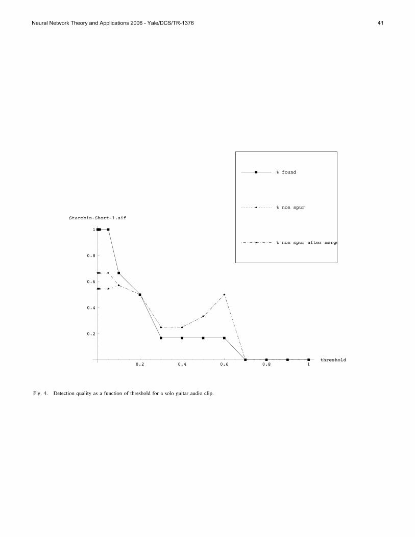
0.2 0.4 0.6 0.8 1threshold
0.2
0.4
0.6
0.8
1
Starobin!Short!1.aif
% non spur after merge
% non spur
% found
Fig. 4. Detection quality as a function of threshold for a solo guitar audio clip.
Neural Network Theory and Applications 2006 - Yale/DCS/TR-1376 41


![Heterogeneous Neural Networks: Theory and Applicationsbelanche/PhDThesis/TLABM3de3.pdf · 2011-11-15 · Heterogeneous Neural Networks: Theory and Applications ... 99d] Belanche,](https://img.pdfslide.us/doc/110x75/5f0d659f7e708231d43a267c/heterogeneous-neural-networks-theory-and-applications-belanchephdthesis-2011-11-15.jpg)