HAL Id: hal-03246585https://hal.archives-ouvertes.fr/hal-03246585

Submitted on 7 Jun 2021

HAL is a multi-disciplinary open accessarchive for the deposit and dissemination of sci-entific research documents, whether they are pub-lished or not. The documents may come fromteaching and research institutions in France orabroad, or from public or private research centers.

L’archive ouverte pluridisciplinaire HAL, estdestinée au dépôt et à la diffusion de documentsscientifiques de niveau recherche, publiés ou non,émanant des établissements d’enseignement et derecherche français ou étrangers, des laboratoirespublics ou privés.

Distributed under a Creative Commons Attribution| 4.0 International License

Neural network prediction of the topside electroncontent over the Euro-African sector derived from

Swarm-A measurementsOla Abuelezz, Ayman Mahrous, Pierre Cilliers, Rolland Fleury, Mohamed

Youssef, Mohamed Nedal, Ahmed Yassen

To cite this version:Ola Abuelezz, Ayman Mahrous, Pierre Cilliers, Rolland Fleury, Mohamed Youssef, et al.. Neu-ral network prediction of the topside electron content over the Euro-African sector derived fromSwarm-A measurements. Advances in Space Research, Elsevier, 2021, 67 (4), pp.1191-1209.�10.1016/j.asr.2020.11.009�. �hal-03246585�

Neural network prediction of the topside electron content overthe Euro-African sector derived from Swarm-A measurements

Ola A. Abuelezz a,⇑, Ayman M. Mahrous a,b, Pierre J. Cilliers c, Rolland Fleury d,Mohamed Youssef a, Mohamed Nedal e, Ahmed M. Yassen a

aSpace Weather Monitoring Center (SWMC), Physics Dept., Faculty of Science, Helwan University, Cairo, Egyptb Institute of Basic and Applied Sciences, Egypt-Japan University of Science and Technology (E-JUST), Alexandria, Egypt

cSouth African National Space Agency (SANSA), Hermanus, South AfricadLab-STICC, UMR 6285, Institut Mines-Telecom Atlantique, Campus de Brest, France

e Institute of Astronomy, Bulgarian Academy of Sciences, Sofia, Bulgaria

This study presents the first prediction results of a neural network model for the vertical total electron content of the topside iono-sphere based on Swarm-A measurements. The model was trained on 5 years of Swarm-A data over the Euro-African sector spanning theperiod 1 January 2014 to 31 December 2018. The Swarm-A data was combined with solar and geomagnetic indices to train the NNmodel. The Swarm-A data of 1 January to 30 September 2019 was used to test the performance of the neural network. The data wasdivided into two main categories: most quiet and most disturbed days of each month. Each category was subdivided into two sub-categories according to the Swarm-A trajectory i.e. whether it was ascending or descending in order to accommodate the change in localtime when the satellite traverses the poles. Four pairs of neural network models were implemented, the first of each pair having one hid-den layer, and the second of each pair having two hidden layers, for the following cases: 1) quiet day-ascending, 2) quiet day-descending,3) disturbed day-ascending, and 4) disturbed day-descending. The topside vertical total electron content predicted by the neural networkmodels compared well with the measurements by Swarm-A. The model that performed best was the one hidden layer model in the case ofquiet days for descending trajectories, with RMSE = 1.20 TECU, R = 0.76. The worst performance occurred during the disturbeddescending trajectories where the one hidden layer model had the worst RMSE = 2.12 TECU, (R = 0.54), and the two hidden layermodel had the worst correlation coefficient R = 0.47 (RMSE = 1.57).In all cases, the neural network models performed better thanthe IRI2016 model in predicting the topside total electron content. The NN models presented here is the first such attempt at comparingNN models for the topside VTEC based on Swarm-A measurements.

Keywords: Neural network; Swarm satellite; Topside vertical electron content; IRI2016 model

1. Introduction

Observations of the topside ionosphere by the Swarm-Asatellite can complement the bottom-side ionospheric mea-surements by ionosondes (Huang and Reinisch, 2001). Thelargest part of the TEC comes from the topside ionosphere(h > hmF2) with contribution estimated to be from 65%(Belahaki and Tsuagori, 2002), to 80% (Bilitza, 2009).

⇑ Corresponding author.E-mail addresses: ola.abuelezz@gmail.com (O.A. Abuelezz), ayman.

mahrous@ejust.edu.eg (A.M. Mahrous), pjcilliers@sansa.org.za (P.J.

Cilliers), rolland.fleury@imt-atlantique.fr (R. Fleury), mnedal@astro.

bas.bg (M. Nedal).

1

Therefore, it is important to establish a topside electroncontent model which may be useful for telecommunicationpurposes.

The ionosphere, being part of the upper atmosphere ofEarth, is a highly variable environment. The ionosphericelectron density varies spatially with altitude and latitude,and temporally with a time of day, season, and solar activ-ity (Wintoft and Cander, 2000). The TEC is an importantionospheric feature that can be used for several purposes,such as the studies of the ionosphere-plasmasphere systemand space weather applications, as well as for Global Nav-igation Satellite Systems (GNSS) applications (Stankovet al., 2010). The TEC, measured along the path of a GNSSradio signal, represents the total number of electrons in acylinder of a 1 m2 cross-sectional area along the path ofthe GNSS radio signal. In general, the slant TEC (STEC)can be calculated by taking the line integral of the three-dimensional electron density (ne) along the signal path (s)from a GNSS receiver to the GNSS satellite (Bothmerand Daglis, 2007). The vertical TEC (VTEC) at the iono-spheric pierce point of the ray path is derived from theSTEC by using a geometric mapping function (Liu et al.,2009).

The ionospheric variability as described by TEC varia-tions has been analysed for magnetically the quiet and dis-turbed days. Negative or positive ionospheric stormsduring disturbed days can be characterized by either adecrease or increase of TEC and electron density withrespect to quiet time behaviour (e.g., Prolss, 1993a, 1995;Fuller-Rowell et al., 1994; Buonsanto, 1999; Tsagouriet al., 2000; Matamba et al., 2015).

It is known that modelling ionospheric TEC during dis-turbed days is a big challenge (Fuller-Rowell et al., 2000;Habarulema, 2010, 2011; Uwamahoro, and Habarulema,2015). Several other researchers have attempted to predictand forecast the TEC during both quiet and disturbed con-ditions (Mao et al., 2005, 2008; Habarulema, 2010; Erchaet al., 2012; Watthanasangmechai et al., 2012).

We have utilized the neural network (NN) techniquethat has been demonstrated by several authors (e.g.,Habarulema and McKinnell, 2012; Habarulema, 2010;Habarulema et al., 2009; Okoh, 2016) as a very efficienttool for ionospheric modelling and forecasting. Thestrengths and versatility of neural NNs are derived fromtheir ability to represent both linear and nonlinear relation-ships between inputs and outputs directly from the inputdata (Baboo and Shereef, 2010).

TEC prediction using the NN technique has been doneover many years with relative success. An artificial NNhas been used in ionospheric studies that applied largeamounts of solar-terrestrial and ionospheric data to predictthe temporal and spatial variations of the ionospheric crit-ical frequency foF2 and TEC Cander, 1998). The MiddleEast Technical University Neural Network (METU-NN)model, a data-driven neural network model of one hiddenlayer, was used for forecasting and nowcasting of TEC val-ues of the ionosphere during space weather events

(Tulunay et al., 2006). The first NN Global PositioningSystem (GPS) prediction model over South Africa basedon TEC measurements was developed by Habarulemaet al. (2009). The model comprised a feed forward neuralnetwork (NN) trained with data from 10 GPS receiver sta-tions over five years. TEC predictions over southern Africawere produced by means of the regional southern AfricaTotal Electron Content Prediction (SATECP) NN modelbased on GPS data (Habarulema et al., 2011). The applica-tion of NN modelling for forecasting the ionospheric TECover China was demonstrated by Song, et al. (2018), usingthe genetic algorithm to optimize the initial weights of theNN. The first regional total electron content (TEC) modelover the entire African region, the AfriTEC model, wasdeveloped by Okoh et al. (2019) using observations foryears 2000 to 2017 from terrestrial GPS receivers andGPS receivers on the COSMIC satellites.

The modelling of topside ionosphere has been attemptedby Coısson et al., (2002) through a comparison of the top-side electron concentration profiles of the IRI and NeQuickmodels with measurements by the Intercosmos-19 satellitefor many different geophysical situations during a periodof high solar activity (March 1979 to December 1980).They concluded that topside modelling of both the IRIand NeQuick needed improvement. Improvements in theBent model for the topside electron density of the IRI wereproposed by Depuev and Pulinets (2004) using the data-base of Intercosmos- 19 satellite topside soundings duringa period of high solar activity. Attempts were made toaccommodate longitudinal dependencies in the empiricalmodel they proposed. The modelling of the electron densityvalues topside ionosphere has been attempted by Pignalberiet al. (2018) using electron density recorded by Swarmsatellites from December 2013 to June 2016 and foF2and hmF2 values provided by IRI UP (International Ref-erence Ionosphere UPdate). They assumed that the scalingheight in the topside region was constant and demonstratedthat the a-Chapman analytical function gave the best per-formance. Topside total electron content (TEC) valuesderived from the GOCE and TerraSAR-X low earth orbitsatellites were used by Ren et al., 2020) to validate the top-side ionosphere predictions of the NeQuick2 and IRI-2016models from 2008 to 2018. Their results showed that thesetwo models both underestimate the topside ionosphere.The variation of the VTEC over Antarctica during 2011–2017 was studied by Tariku (2020). The pattern of varia-tion of the VTEC inferred from the IRI 2016, IRI-Plas2017 and NeQuick 2 models was demonstrated to be gen-erally smaller than the GPS-derived VTEC values. Fromthe literature, it is clear that there is a gap on modellingof the topside VTEC.

In this work, we introduce the first regional Swarm-NNmodel for VTEC in the topside ionosphere trained over theEuro-African sector using data over the period from Jan-uary 2014 to December 2018 and tested with Swarm-Adata from 1 January to 30 September 2019. Particularly,we have utilised the NN technique to describe the quiet

2

and disturbed periods of VTEC obtained from Swarm-Asatellite measurements through the ascending and descend-ing trajectories. In Section 2, we describe the data andmethods used in the study. In Section 3, we present theresults and discussion and the comparison of the neuralnetwork model with the IRI2016 model. In Section 4, wepresent the conclusion of the study.

2. Data and methodology

Data used in this work include topside electron contentvalues at a temporal resolution of 1 sec that were derivedfrom Swarm-A data, as well as solar and geomagneticindices obtained from the OMNI database.

2.1. Data

2.1.1. Swarm satellite

Swarm is a recent mission of the European Space Agency(ESA) that was launched in November 2013 with the aim ofstudying the dynamics of the Earth’s magnetic field and itsinteractions with the Earth system. It consists of a constella-tion of three satellites (Swarm-A, -B and -C). The threeSwarm satellites fly in the topside ionosphere. Each satellitehas an on-board GPS receiver of which the data can be usedfor deriving the topside ionospheric TEC along the ray pathbetween the SwarmandGPS satellites (Zakharenkova,Asta-fyeva 2015). SwarmA and C fly at an altitude of 460 kmwitha 1.5� longitudinal spacing and an inclination of 87.4�.Swarm B flies at an altitude of 540 km with an inclination86.8�. During a day, the Swarm satellites complete about15 to 17 polar orbits in an average 90min per orbit. The orbi-tal planes of Swarm-B and Swarm-A/C differ by 9 h of localtime (Fiori et al., 2013; 2014). Swarm satellites regress in lon-gitude around 23� between orbital ascending nodes. Swarm-A and -C need about 133 days to cover all 24 h of local timeandSwarm-Bneeds about 141days (Xiong et al., 2016b). Thelocal time remains almost the same across most of the lati-tudes in each crossing on a particular day during the ascend-ing or descending trajectories. Data sets measured by Swarmcan be downloaded from (http://earth.esa.int/Swarm). Thecadence of L2-TEC data is 1 Hz.

One Swarm satellite can communicate simultaneouslywith multiple GNSS satellites; hence, there can be multipleSTEC values for a given universal time (UT) (Swarm,2013). The Swarm VTEC is derived from the mean of theSwarm STEC values (Zakharenkova and Astafyeva,2015). The topside VTEC is here modelled and predictedas a function of physical and geophysical parameters thatinclude season (day of year), time of day, as well as solarand geomagnetic activities.

2.1.2. Solar and geomagnetic indices

The solar wind data and geomagnetic indices wereobtained from the OMNI database (http://omniweb.gsfc.nasa.gov/) during the descending phase of the solarcycle 24. Data from 2014 to 2018 were used for training

our model, whereas data of 2019 were used for testingthe performance of the model. The solar and geomagneticinputs for the NN included the solar radio flux density atwavelength 10.7 cm (F10.7 index), and the disturbed stormtime (Dst) index. The Dst index is a scale of geomagneticactivity used to express the acuteness of magnetic storms.The ten most quiet days and the five most disturbed daysin each month were selected based on the Dst index byusing the sequence of the degree of quietness and distur-bance numbered as follows 1q, 2q, 3q, 4q, 5q, 6q, 7q, 8q,9q and 0q, and 1d, 2d, 3d, 4d and 5d, respectively(http://wdc.kugi.kyoto-u.ac.jp/qddays/format.html).

The F10.7 index is a daily measurement indicator forsolar activity, given in solar flux units (s.f.u.), and variesfrom (50 � F10.7 � 300) through a solar cycle. To repre-sent influence of the solar wind on TEC, the proton fluxesat the L1 point in three energy bands (i.e 10, 30, 60 MeV)are also used as inputs to the NN.

2.2. Methodology

Pre-processing of Swarm-A data involved the extractionof VTEC values from STEC between Swarm-A and GPSaltitudes. The Swarm-A STEC values are along the raypaths from Swarm-A satellite to the GPS satellites. Thereare typically five GPS satellites in view at each epoch.The VTEC value at each 1 sec epoch is derived from themean of the STEC values by using a geometric mappingfunction for each satellite.

After that, The VTEC values are selected for elevation>50� as recommended in the Swarm Level 2 TEC productdescription.

1- We separated the ascending and descending trajecto-ries of the Swarm-A passes, because they occurred attwo different local times e.g. ascending and descend-ing at 10:20 LT and 22:22 LT respectively on 2017–09-06 over the African sector.

2- We filtered the data by geographic longitude and lat-itude to cover the Euro-African region, defined by thecoordinate bounds �71.5 < latitude < 71.5 and�20 < longitude < 50.

We inspected the correlation between potential inputvariables and Swarm VTEC values and used a correlationmatrix to select only nine inputs. The 9 input parameterswere selected from the error matrix, which demonstratesthe performance of the model. The error matrix is oftenused in the field of machine learning for classification prob-lems (see Stehman, 1997; Powers, 2011). It shows howmuch each predicted class is correlated with its correspond-ing drivers. The 9 input parameters were taken as the dayof the year (DOY), the hours of the day rounded to thenearest integer (HR), latitude, longitude, Dst index,F10.7 index, and the proton fluxes at 10, 30, and60 MeV. To convert the seasonal and diurnal variationsinto numerically continuous parameters, the DOY and

3

HR are split into two cyclical components defined by(Habarulema, 2010)

DOY s ¼ sin2p� DOY

365:25

� �

DOY c ¼ cos2p� DOY

365:25

� �

HRs ¼ sin2p� HR

24

� �

HRc ¼ cos2p� HR

24

� �

ð1Þ

where DOYs, DOYc, HRs, and HRc are the sine andcosine components of the DOY and HR, respectively.Therefore, 11 input parameters were used in the final NNmodel, namely DOYs, DOYc, HRs, HRc, latitude, longi-tude, Dst, F10.7, PF 10 MeV, PF 30 MeV, and PF60 MeV. Before the training of the NN model, the datasetwas divided into two categories for training and testingpurposes. Each category was spilt corresponding to theionospheric variability (e.g. quiet and storm conditions).Furthermore, each category showed the latitude, longitudeand HR dependency through separating the ascending anddescending trajectories of Swarm-A.

The quietest and the most disturbed days of each monthwere derived from the WDC database (http://wdc.kugi.ky-oto-u.ac.jp/). The time resolution of the measured topsideVTEC is 1 s and the actual topside VTEC that obtainedfrom Swarm-A data were extracted for a period of fiveyears (2014, 2015, 2016, 2017 and 2018) from the datasetand used in NN training process. Then data from the first9 months of 2019 were used for testing the NN perfor-mance. This procedure is to make sure that the NN wasnot being over-trained but sufficiently generalized.

We tested two NN architectures for each relationship: aNN with a single hidden layer and NN with double hiddenlayers, with 20 hidden nodes each. The single hidden layer(1HL) NN refers to a NN with only one hidden layer,besides the input and output layers. The two hidden layer(2HL) NN refers to a NN with two hidden layers, besidesthe input and output layers.

After inspecting the correlation of the VTEC values withdifferent potential inputs we selected only 11 input param-eters that had the highest correlations with the VTEC val-ues. The numbers of daily data sets used for training andtesting for the quiet days ascending (QD Asc), quiet daysdescending (QD Des), disturbed days ascending (DDAsc), and disturbed days descending (DD Des) are shownin Table 1.

In a few cases, there was no Swarm data available on thedisturbed days or quiet days of some months in the year.

2.3. The neural network model

The NN consists of a number of processing units calledneurons or perceptrons linked by weighted connectionsbetween the layers (Hopfield, 1982). Each unit receivesinputs from other units in the previous layer and generatesa single output. The output is then forwarded as an inputto all the other neurons in the subsequent layers. NNs con-sist of three main sections (Fig. 1); the input layer, whichinterfaces with the input variables, the hidden layer(s),where the learning process is performed, and the outputlayer which includes the target variable. The layers in amultilayer neural network are fully connected, that is,every neuron in each layer is connected to every other neu-ron in the subsequent layer. The NN is considered as aniterative learning process in which it maps the embeddedrelation between the inputs and the output when givenenough training examples.

The NN performance strongly depends on the NNarchitecture and it is different from one application toanother. The number of hidden layers and hidden neu-rons depends on the complexity of the problem understudy, but can lead to overfitting in which the model is

Table 1

Number of quiet days (QD) (on average 10 days per month) and disturbed days (DD) (on average 5 days per month) for ascending (Asc) and descending

(Des) passes per year for each year of Swarm-A data used.

Training Data Testing Data

2014 2015 2016 2017 2018 2019

Asc Des Asc Des Asc Des Asc Des Asc Des Asc Des

QD 119 119 120 120 120 120 120 120 119 119 86 86

DD 58 58 59 59 60 60 60 60 60 60 45 45

Fig. 1. Illustration of the NN architecture with labelled inputs and

output.

4

closely fit to the training data but fails to fit the testingdata. So, an efficient NN model is characterized by theability to be generalized over a wide range of data ithas not encountered before. Yet, there is no simple rulethat can determine the optimum number of hidden layersand hidden neurons for an application. The architecture/-topology used is determined by trial and error, and thebest architecture/topology in the present case was chosenas the one with the lowest RMSE over the period of inter-est. The output of a single-hidden layer NN can be writ-ten as

Gk ¼ fX

M

j¼1

H jwð2Þj;k þ bk

!

ð2Þ

where Gk is the network output at the k-th output of K out-put nodes, M the number of hidden nodes in the first hid-

den layer, wð2Þj;k the weights of the links between the j-th

hidden node and the k-th output node, bk the biases con-nected to the output nodes, f the activation function, andHj the output of the j-th hidden node, which can be repre-sented as

H j ¼ fX

N

i¼1

xiwð1Þi;j þ bj

!

ð3Þ

where xi the input values, N the number of inputs nodes,

wð1Þi;j the weights of the links between the i-th input and

the j-th node of the first hidden layer, and bj the biases con-nected to the first hidden layer. For a double-hidden layersNN, the output can be written as

yl ¼ fX

S

k¼1

Gkwð3Þk;l þ bl

!

ð4Þ

where yl is the output of the l-th output node, Gk representthe outputs of the previous hidden layer, S the number of

hidden nodes in the second hidden layer, wð3Þk;l the weights

of the links between the k-th hidden node of the secondhidden layer and the l-th output node, and bl the bias con-nected to the l-th output nodes.

We used a semi-automatic method to find the best archi-tecture for any specific regression problem. This methodinvolves using two nested for-loops in which the numberof loops represents the number of hidden layers and eachloop represents the number of hidden neurons in this speci-

Fig. 2. The Dst index (nT) and the F10.7 index (sfu) and the solar proton fluxes at 3 energy channels (PF > 10 MeV, PF > 30 MeV, and PF > 60 MeV)

during the last 10 years. The time period spans from 1 January 2014 to 30 September 2019. All data are 1-hour-averaged data from the OMNIWeb Service.

5

fic hidden layer. Each NN topology runs two consecutivetimes to estimate the average response of this particularNN architecture. The Root-Mean-Squared Error (RMSE)and the percentage error are recorded for each NN topol-ogy and we selected the NN topologies that gave the min-imum errors.

We chose the feed-forward back-propagation NN as it isone of the most popular approaches of machine learningand it performs quite effectively for space weather applica-

tions (see Qahwaji and Colak, 2006; Ajabshirizadeh et al.,2011; Bortnik et al., 2018). Besides, it can approximate anyinput–output map with concurrent inputs and outputs effi-ciently (see Haykin, 1999; Bakr and Negm, 2012). We usedthe Levenberg-Marquardt optimization (Levenberg, 1944;Marquardt, 1963) as a learning rule for our model becauseit performed better than other training functions for ourapplication. The training process in the back-propagationalgorithm of a neural network involves two phases, namely

Fig. 3. (a,b). Comparison between the observed and predicted VTEC during ascending (a, QD Asc) and descending (b, QD Des) passes of Swarm-A on

geomagnetically quiet days. The observed VTEC was derived from Swarm-A and the predicted VTEC was derived from NN models with one hidden layer

(1HL) and two hidden layers (2HL) respectively.

6

forward and backward. The back-propagation algorithm isassumed to converge when the error per iteration (i.e.,epoch) is satisfactorily small.

To assess the performance of the NN, RMSE was com-puted. The RMSE is defined as

RMSE ¼

ffiffiffiffiffiffiffiffiffiffiffiffiffiffiffiffiffiffiffiffiffiffiffiffiffiffiffiffiffiffiffiffiffiffiffiffiffiffiffiffiffiffiffiffiffiffiffiffiffiffiffiffiffi

P

N

i¼1

ðVTECmeas � VTECpredÞ2

N

v

u

u

u

t

; ð5Þ

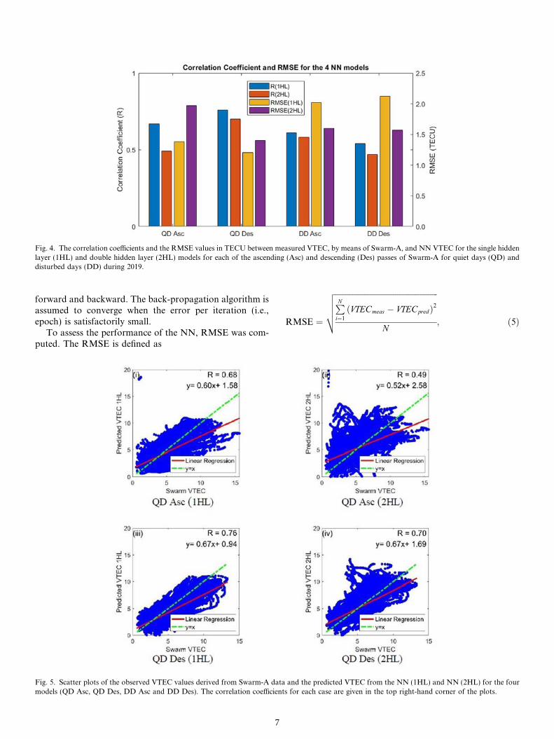
Fig. 4. The correlation coefficients and the RMSE values in TECU between measured VTEC, by means of Swarm-A, and NN VTEC for the single hidden

layer (1HL) and double hidden layer (2HL) models for each of the ascending (Asc) and descending (Des) passes of Swarm-A for quiet days (QD) and

disturbed days (DD) during 2019.

Fig. 5. Scatter plots of the observed VTEC values derived from Swarm-A data and the predicted VTEC from the NN (1HL) and NN (2HL) for the four

models (QD Asc, QD Des, DD Asc and DD Des). The correlation coefficients for each case are given in the top right-hand corner of the plots.

7

where N is the number of data points, VTECpred is VTECpredicted by the NN and VTECmeas is the VTEC derivedfrom Swarm-A measurements.

The Pearson correlation coefficient (R) between theSwarm and NN (VTEC) as given by

R ¼nðRxyÞ � ðRxÞðRyÞ

ffiffiffiffiffiffiffiffiffiffiffiffiffiffiffiffiffiffiffiffiffiffiffiffiffiffiffiffiffiffiffiffiffiffiffiffiffiffiffiffiffiffiffiffiffiffiffiffiffiffiffiffiffiffiffiffiffiffi

½nRx2 � ðRxÞ2�½nRy2 � ðRyÞ2�

q ð6Þ

was used as additional measure of the performance of theNN. Here the numerator is the covariance between thevariables x and y and the denominator is the product ofthe standard deviation of x and y. The best NN architec-ture was taken as the one with the minimum RMSE andhighest correlation coefficient over the whole period ofinterest for the selected dataset.

3. Results and discussion

This section describes the results of the NN and predict-ing topside VTEC values over the Euro-African region.The dataset was derived from Swarm-A measurements dur-ing the period 1 January 2014 to 30 September 2019. Thetime series were divided into two periods for each of fourmodels. The data for the period 2014 – 2018 were usedfor training the NN and from 1 January 2019 to 30 Septem-

ber 2019 were used for testing the predicted topside VTECvalues.

Fig. 2 shows the Dst index, the F10.7 index, and thesolar proton fluxes in three energy channels for the fullsolar cycle from 2009 to 2019. The green parts show theperiod preceding the launch of the Swarm satellites to pro-vide the context of the data used for training the NN. Theperiods used for training and testing of the NN are shownin red and blue respectively. The highest levels of protonflux in all 3 energy channels occurred during the storm of7 September 2017 when the Dst index reached �124 nTand F10.7 reached 185.5 sfu, namely Proton flux(>10 MeV) = 1208 per cm2-sec-ster, Proton flux(>30 MeV) = 404 per cm2-sec-ster and Proton flux(>60 MeV) = 142 per cm2-sec-ster. The training data cov-ered half of the solar cycle and started near the peak of thesolar cycle while the testing data was taken from the end ofthe solar cycle. Note that while the training data includedseveral strong storms (Dst � - 150 nT), the testing datahad no strong storms (Dst � - 50 nT, Pf � 0.36 MeV),Since Dst hardly went below �50 nT as well as very lowproton flux levels. This might have contributed to the factthat the DD models had lower correlations and higherRMSE values in general compared to QD models.

Fig. 3(a) and (b) show the time-series graphs of the com-parison between the measured and estimated VTEC from

Fig 5. (continued)

8

January to September 2019 for the single hidden layer NN(1HL) and the double hidden layer NN (2HL).

The measured topside VTEC is obtained from Swarm-A. The x-axis in Fig. 3 represents 9 months of year 2019,which was used as the testing set. The x-axis is labelled‘‘Index” because it is chronological but not sequential intime. Hence, there is no direct link between the index andthe day of the month. The results are labelled by themonths which represent the solstices and equinoxes of theyear by the following periods: (‘‘Jan-Feb” represents thesolstice period 1 January to 28 February 2019), (‘‘Mar-May” represents the equinox period 1 March to 31 May2019), (‘‘Jun-Aug” represents the solstice period 1 June to31 August 2019), (‘‘Sep” represents the equinox period 1September to 30 September 2019). We have avoided the

word ‘‘season” since every pass of the Swarm satellite overthe Euro-African sector traverses both northern and south-ern hemispheres, which have opposite seasons. In the toppanel, the LT is shown at the transitions between theseperiods. This format of the results facilitates comparisonof the overall the variations of the range of VTEC valuesduring different part of the testing year.

The local time (LT) difference between the ascendingand descending passes is about 12 h. Note that, betweentwo successive ascending equatorial crossings of Swarm-A, the LT decreases by 1.28 min and the longitudedecreases by about 23� (Xiong et al., 2016b).

Fig. 3 shows the strong dependency of the diurnalVTEC variation on the LT. The largest variation of thetopside VTEC (16 TECU) occurs between noon and dusk

Fig. 6. Topside VTEC along the Swarm-A passes together with corresponding VTEC from the NN and IRI2016 models for Quiet Day Ascending passes

(QD Asc).

9

and the least variations (5 TECU) occurs between midnightand dawn.

For example, during the Sep equinox during 2019, thelargest VTEC variations occur during the ascending trajec-tories with LT variations decreasing from 18:00 to 14:00(afternoon). During the same period, the VTEC variationsalong the descending trajectories are 6 TECU with LT vari-ations decreasing from 06:00 to 02:00 (pre-dawn). Duringthe other periods of the year similar patterns, occur of largeand small VTEC variations during the daytime and night-time passes respectively.

Throughout the testing period, the VTEC variationspredicted by the NN model are synchronized with the mea-sured VTEC and follows the trend of the observations.

The performance of the four models is summarized inFig. 4. This figure shows that the model that performedbest was the one hidden layer model in the case of quiet

days for descending trajectories model (QD Des (1HL)),with RMSE = 1.20 TECU, and correlation coefficientR = 0.76. The worst performance as measured by RMSEoccurred during the disturbed descending trajectories forone hidden layer model (DDDes (1HL)) with RMSE= 2.12TECU and R = 0.54. The worst performance as measuredby correlation coefficient occurred during the disturbeddescending trajectories for the two hidden layer model(DD Des (2HL) with R = 0.47 and RMSE = 1.57 TECU.

Fig. 5 shows scatter plots, linear regression lines and thecorrelation coefficients between the observed VTEC valuesderived from Swarm-A data and the predicted VTEC valuesfrom theNN (1HL) andNN (2HL) for the fourmodels in thefollowing order QD Asc, QD Des, DD Asc and DD Des.

In each case, the correlation coefficient as well as theequation for the linear regression line and the ideal pre-diction line (y = x) are given. The NN models underesti-

Fig 6. (continued)

10

mate the measurements. The model with the best correla-tion coefficient is not the same as the model for which thelinear regression is closest to the ideal prediction line. Thebest linear regression occurs with the DD Asc (1HL)model (y ¼ 0:72X þ 1:55) and the worst linear regressionoccurs with the DD Des (2HL) model((y ¼ 0:38X þ 2:95).

Figs. 6–9 show typical comparisons of topside VTECfrom Swarm-A, NN and IRI2016 model for selected casesand passes of Swarm-A during the four periods of the year(March and September equinoxes , January and Junesolstices).

Each of the 16 panels of Figs. 6–9 show colour codedvalues of the measured VTEC along the tracks of

Swarm-A and the corresponding modelled VTEC derivedfrom NN(1HL),NN(2HL) and IRI2016 models. The 16panels are arranged according to four periods (the twoequinoxes March and September, the two solstices Januaryand June) each with examples of VTEC from the threemodels (NN(1HL),NN(2HL), and IRI2016) compared toSwarm-A VTEC. In each case, the comparisons are orga-nized by DOY.

The VTEC derived from IRI2016 model was calculatedalong fixed longitudes namely the longitude where theSwarm-A paths crossed the geographic equator. The devi-ation of the Swarm path from this fixed longitude over theEuro-African sector is at most 2.6� (due to the inclinationof the Swarm-A orbit being 87.4�).

Fig. 7. Topside VTEC along the Swarm-A passes together with corresponding VTEC from the NN and IRI2016 models for Quiet Day Descending passes

(QD Des).

11

The maps in Figs. 6–9 clearly display the dependence ofthe VTEC distribution on longitude and LT.

In all the selected cases, the NN models performed bet-ter than the IRI2016 model that frequently had an equato-rial dip in the topside VTEC which was not matched by theSwarm-A measurements. The predictions of the IRI2016model, in most cases, underestimates the Swarm-A VTEC.

The largest differences between the NN models andIRI2016 model occurred at midnight and during the earlymorning, while the differences were smaller during thedaytime.

3.1. The QD Asc model

Fig. 6 illustrates the topside VTEC along the Swarm-Apasses together with corresponding VTEC from the NN(QD Asc) and IRI2016 models.

Panel (i) of Fig. 6 shows the QD Asc daytime paths(LT = 10:48) during the Jan-Feb solstice (represented byDOY 47). Note that the best prediction of the VTEC forthis day is along the central path over Africa (10�) whereboth models fit the Swarm-A measurements equally well.The NN (1HL) model matches the Swarm-A better thanthe NN (2HL) along the western longitude (�13�), whilethe reverse occurs at the eastern longitude (34�) wherethe NN (2HL) model predicts a better match with the mea-sured VTEC than the NN (1HL). It is not clear why thetwo NN models have different performances in the easternand western paths over Africa. The IRI2016 model is worsethan the NN model because it shows two VTEC peaks oneither side of the geomagnetic equator and underestimatesthe VTEC values at mid latitudes.

Panels (ii) and (iii) of Fig. 6 show the QD Asc nighttimepaths (LT = 02:43 and LT = 21:04 respectively) during the

Fig 7. (continued)

12

Mar-May equinox (represented by DOY 137) and the Jun-Aug solstice (represented by DOY 199). The predictions ofthe VTEC for these days by the NN (1HL) and NN (2HL)models closely match the Swarm-A measurements overAfrica. Note the hemispheric asymmetry of VTEC; VTECabove 6 TECU only occurred on northern hemisphere midlatitudes on these days. The IRI2016 model predictsVTEC < 2 TECU during all 3 paths during these days.Thus significantly underestimating Swarm VTEC.

Panel (iv) of Fig. 6 shows the QD Asc daytime paths(LT = 15:24) during the Sep equinox (represented byDOY 262). Note that the best prediction of the VTECfor this day is by the NN (1HL) model along the westernpath over Africa (�15�).

The IRI2016 model predicted almost identical double-peak VTEC distributions for all 3 paths over Africa andunderestimated the measured values by 3 TECU.

3.2. The QD Des model

Fig. 7 illustrates the topside VTEC along the Swarm-Apasses together with corresponding VTEC from the NN(QD Des) and IRI2016 models.

Panel (i) of Fig. 7 shows the QD Des nighttime paths(LT = 22:29) during the Jan-Feb solstice (represented byDOY 50). Note that the both The NN (1HL) and theNN (2HL) models give good predictions of the VTECfor this day along the eastern path over Africa (41� E) asthe VTEC values closely match that of Swarm. On the

Fig. 8. Topside VTEC along the Swarm-A passes together with corresponding VTEC from the NN and IRI2016 models for Disturbed Day Ascending

passes (DD Asc).

13

other two paths of Swarm-A the NN (2HL) model givesslightly better estimates of VTEC values than the NN(1HL) model. The IRI2016 model predicts VTEC valueslower than half of the measured values during all 3 pathsduring this day. During all 3 Swarm-A paths the peaksof VTEC seem to occur at the geomagnetic equator (10�N geographic), whereas the 1HL and 2HL models predictpeak at around the geographic equator.

Panels (ii) of Fig. 7 shows the QD Des daytime paths(LT = 14:13) during the Mar-May equinox (representedby DOY 142). The predictions of the VTEC for this dayby the NN (1HL) and NN (2HL) models closely matchthe Swarm-A measurements over Africa. At this LT thelongitudinal variations of the VTEC is minimal. TheIRI2016 predicts 2 VTEC peaks on all 3 paths over Africa,one peak at the geomagnetic equator and the other peak inthe southern hemisphere at about 20� S (geographic),

while Swarm VTEC shows an extended peak covering lat-itudes from about �10 to 30�.

Panels (iii) of Fig. 7 shows the QD Des daytime paths(LT = 10:50) during the Jun-Aug solstice (represented byDOY 180). The predictions of the VTEC for this day bythe NN (1HL) and NN (2HL) models are similar to theSwarm-A measurements over Africa. The IRI2016 modelpredicts the peaks of the VTEC to be in the southern hemi-sphere during all 3 paths during this day that is inconsistentwith the Swarm-A measurements.

Panel (iv) of Fig. 7 shows the QD Des nighttime paths(LT = 03:54) during the Sep equinox (represented byDOY 257). Note that the predictions of the VTEC for thisday by the NN (1HL) and NN (2HL) models are similar tothe Swarm-A measurements over Africa and they have lowvalues (�5 TECU). The IRI2016 model underestimates themeasured values by 5 TECU.

Fig 8. (continued)

14

3.3. The DD Asc model

Fig. 8 illustrates the topside VTEC along the Swarm-Apasses together with corresponding VTEC from the NN(DD Asc) and IRI2016 models.

Panel (i) of Fig. 8 shows the DD Asc daytime paths(LT = 14:34) during the Jan-Feb solstice (represented byDOY 5). Note that the NN (2HL) model provides the bestprediction of the VTEC for this day. The NN (1HL) modeloverestimates the VTEC values along the central and east-ern longitudes (24� and 0� respectively). The IRI2016model predicts VTEC values lower than the measured val-ues during all 3 paths during this day. In addition, theIRI2016 shows 2 VTEC peaks, the largest of which occursat 10� S geographic, whereas the Swarm only show oneVTEC peak.

Panels (ii) of Fig. 8 shows the DD Asc nighttime paths(LT = 03:16) during the Mar-May equinox (representedby DOY 131). Note that the best prediction of the VTECfor this day is by the NN (2HL) model. The NN (1HL)model overestimates the VTEC Swarm-A values alongthe central and eastern longitudes (33� and 10� respec-tively). The IRI2016 predicts VTEC below 1 TECU in allpaths, thus significantly underestimating Swarm VTEC.

Panels (iii) of Fig. 8 shows the DD Asc daytime paths(LT = 19:22) during the Jun-Aug solstice (represented byDOY 218). Note that the NN (2HL) model provides thebest prediction of the VTEC for this day. The NN (1HL)model over estimates the VTEC Swarm-A values alongall 3 longitudes. The IRI2016 model predicts VTEC valueslower than half of the measured values during all 3 pathsduring this day.

Fig. 9. Topside VTEC along the Swarm-A passes together with corresponding VTEC from the NN and IRI2016 models for Disturbed Day Descending

passes (DD Des).

15

Panel (iv) of Fig. 8 shows the DD Asc nighttimepaths (LT = 17:01) during the Sep equinox (representedby DOY 244). The predictions of the VTEC for thisday by the NN (1HL) and NN (2HL) models closelymatch the Swarm-A measurements over Africa. TheIRI2016 model underestimates the measured values by4 TECU and erroneously predicts two VTEC peaks inthe northern hemisphere during all 3 paths during thisday.

3.4. The DD Des model

Fig. 9 illustrates the topside VTEC along the Swarm-Apasses together with corresponding VTEC from the NN(DD Des) and IRI2016 models.

Panel (i) of Fig. 9 shows the DD Des nighttime paths(LT = 00:20) during the Jan-Feb solstice (represented byDOY 31). Note that the NN (2HL) model gives the bestprediction with RMSE = 1.99 TECU, while the NN(1HL) model overestimates the VTEC values withRMSE = 2.87 TECU. The IRI2016 model greatly underes-timates Swarm VTEC as it over both paths.

Panel (ii) of Fig. 9 shows the DD Des at the dusk paths(LT = 18:46) during the Mar-May equinox (represented byDOY 95). The predictions of the VTEC for this day by theNN (1HL) and NN (2HL) models closely match theSwarm-A measurements over Africa. At this LT the longi-tudinal variations of the VTEC is minimal. The IRI2016predicts 2 VTEC peaks on all 3 paths over Africa, one peakat the geographic equator and the other peak in the south-

Fig 9. (continued)

16

ern hemisphere at about 20�S, while Swarm only observedone VTEC peak.

Panels (iii) of Fig. 9 shows the DD Des daytime paths(LT = 09:84) during the Jun-Aug solstice (represented byDOY 191). The predictions of the VTEC for this day bythe NN (1HL) and NN (2HL) models are very differentfrom the Swarm-A measurements over Africa.

Panel (iv) of Fig. 9 shows the DD Des nighttime paths(LT = 04:37) during the Sep equinox (represented byDOY 252). Note that the predictions of the VTEC for thisday by the NN (2HL) model is much better than the NN(1HL) model. The NN(2HL) model is generally better thanthe NN(1HL) model for disturbed days (except for theMar-May equinox) probably because the extra layer inthe NN(2HL) model improves the ability of the model tohandle the complexity of the ionosphere during the dis-turbed days. The peaks of the IRI2016 model matchesthe measured VTEC at the geographic equator.

The best performance of the NN models occurred at dif-ferent local times, but in all cases during the equinoxmonths: The QD Asc NN (2HL) model performed bestduring the March equinox at LT = 02.43 (RMSE = 0.56TECU), the QD Des NN (1HL) model performed best dur-ing the September equinox at LT = 15.41 (RMSE = 0.76TECU), the DD Asc NN (2HL) model gave the best per-formance during the March equinox at LT = 3.26(RMSE = 0.90 TECU), and the DD Des NN (1HL) modelalso performed best during the March equinox, but atLT = 10.95 (RMSE = 1.34 TECU). All local times werecovered by the Swarm-A satellite over the four years oftraining data.

Table 2 shows a summary of the RMSE for all results inFigs. 6–9 organized by period of observation and NNmodels.

4. Conclusion

The NN models presented here is the first such attemptat comparing NN models for the topside VTEC based onSwarm-A measurements.

The NN trained on Swarm-A measurements of VTECand geophysical inputs provided useful predictions of thetopside VTEC. The single hidden layer NN performed bet-ter in the case of quiet days for both ascending anddescending trajectories, while the double hidden layerNN performed better in the case of disturbed days for bothtrajectories. This is true when looking at both RMSE and

correlation. These results might imply that the relationbetween the input parameters and the VTEC values duringthe disturbed days is more complex and hence the NN mayneed an additional hidden layer to be able to converge to asmaller error than that which was obtained with the 1HLand 2HL models.

The 11 input parameters (DOYs, DOYc, HRs, HRc, lat-itude, longitude, Dst, F10.7, PF 10 MeV, PF 30 MeV, andPF 60 MeV) proved to be adequate. We investigated theAp index as an additional input parameter, but it gaveworse results.

Comparisons of the NN models with the topside VTECcalculated by means of the IRI2016 model, with measuredF10.7 as optional input, demonstrated that both the NNmodels in all cases performed significantly better than theIRI2016 model. The IRI model frequently had an equato-rial dip in the topside VTEC that was not matched by theSwarm–A measurements.

Future work will include testing the contribution of eachof the input parameters to the accuracy of the predictions.The use of additional hidden layers to improve the NNmodels for disturbed days (DD Asc and DD Des) will beinvestigated. Validations will be performed with otherinstruments including incoherent scattering radars.

The validation period corresponded to a low solar activ-ity. In future, a more comprehensive validation may be per-formed by selecting periods that represent both high andlow solar activity.

Declaration of Competing Interest

The authors declare that they have no known competingfinancial interests or personal relationships that could haveappeared to influence the work reported in this paper.

Acknowledgment

The authors acknowledge the ESA Swarm team for theSwarm mission and for providing the Swarm data via the ser-ver for Swarm data distribution (ftp://Swarm-diss.eo.esa.int).The WDC team in Kyoto are acknowledged for maintainingthe Most Quiet and Disturbed days of each month via thewebsite (http://wdc.kugi.kyoto-u.ac.jp/qddays/index.html).The OMNI web is acknowledged for providing the Ap andDst indices and the F10.7 solar radio flux, and solar protondata on the website (http://omniweb.gsfc.nasa.gov/). Weacknowledge the Community Coordinated Modeling Center

Table 2

The RMSE for all results in Figs. 6–9. All RMSE values are expressed in TECU.

Jan-Feb Solstice Mar-May Equinox Jun-Aug Solstice Sep Equinox

NN (1HL) NN (2HL) IRI2016 NN 1HL NN 2HL IRI2016 NN 1HL NN 2HL IRI NN 1HL NN 2HL IRI

QD Asc 1.45 1.84 2.96 0.86 0.56 3.87 1.22 0.89 3.58 2.65 4.12 2.90

QD Des 1.66 1.46 4.17 0.79 0.80 2.79 1.01 1.19 2.79 0.76 1.26 3.71

DD Asc 1.78 1.55 3.13 1.34 0.90 3.96 2.20 0.97 3.67 1.49 1.41 3.62

DD Des 2.87 1.99 4.89 1.34 1.43 2.36 1.55 1.41 4.22 2.43 1.45 2.56

17

(CCMC) through their public Runs on Request system(http://ccmc.gsfc.nasa.gov for the IRI2016 Model. TheIRI2016 online was developed by the (Dieter Bilitza andIRI team).

References

Ajabshirizadeh, A., Jouzdani, N.M., Abbassi, S., 2011. Neural network

prediction of solar cycle 24. Res. Astron. Astrophys. 11 (4), 491.

Baboo, S.S., Shereef, K.I., 2010. An efficient weather forecasting system

using artificial neural network. Int. J. Environ. Sci. Technol. 1 (4), 321–

326.

Bakr, M.H., Negm, M.H., 2012. Modeling and design of high-frequency

structures using artificial neural networks and space mapping.

Advances in Imaging and Electron Physics, vol. 174. Elsevier, pp.

223–260.

Belehaki, A., Tsagouri, I., 2002. Investigation of the relative bottom-

side/topside contribution to the total electron content estimates. Ann.

Geophys. 45 (1), 73–86. https://doi.org/10.4401/ag-3498.

Bortnik, J., Chu, X., Ma, Q., Li, W., Zhang, X., Thorne, R.M., Spence, H.

E., 2018. Artificial neural networks for determining magnetospheric

conditions. In: Machine Learning Techniques for Space Weather.

Elsevier, pp. 279–300.

Bothmer, V., Daglis, I.A., 2007. Space Weather: Physics and Effects, 213,

315–318, 438 pp., Praxis Publishing Ltd., Chichester, UK.

Bilitza, D., 2009. Evaluation of the IRI-2007 model options for the topside

electron density. Adv. Space Res. 44 (6), 701–706. https://doi.org/

10.1016/j.asr.2009.04.036.

Buonsanto, M.J., 1999. Ionospheric storms – a review. Space Sci. Rev. 88

(3–4), 563–601.

Cander. R., 1998. Artifficial NN Applications in ionospheric studies.

Coısson, P., Radicella, S.M., Nava, B., 2002. Comparisons of experimen-

tal topside electron concentration profiles with IRI and NeQuick

models. Ann. Geophys. 45 (1).

Depuev, V.H., Pulinets, S.A., 2004. A global empirical model of the

ionospheric topside electron density. Adv. Space Res. 34 (9), 2016–

2020.

Ercha, A., Zhang, D., Ridley, A.J., Xiao, Z., Hao, Y., 2012. A global

model: Empirical orthogonal function analysis of total electron

content 1999–2009 data. J. Geophys. Res. 117, A03328. https://doi.

org/10.1029/2011JA017238.

Fiori, R.A.D., Boteler, D.H., Burchill, J., Koustov, A.V., Cousins, E.D.P.,

Blais, C., 2013. Potential impact of Swarm electric field data on global

2D convection mapping in combination with SuperDARN radar data.

J. Atmos. Sol.-Terr. Phys. 93, 87–99. https://doi.org/10.1016/

j.jastp.2012.11.013.

Fiori, R.A.D., Boteler, D.H., Koustov, A.V., Knudsen, D., Burchill, J.K.,

2014. Investigation of localized 2D convection mapping based on

artificially generated Swarm ion drift data. J. Atmos. Sol. Terr. Phys.

114, 30–41. https://doi.org/10.1016/j.jastp.2014.04.004.

Fuller-Rowell, T., Codrescu, M., Moffett, R., Quegan, S., 1994. Response

of the thermosphere and ionosphere to geomagnetic storms. J.

Geophys. Res.: Space Phys. 99 (A3), 3893–3914.

Fuller-Rowell, T., Codrescu, M., Wilkinson, P., 2000. Quantitative

modelling of the ionospheric response to geomagnetic activity. Ann.

Geophys. 18 (7), 766–781.

Habarulema, J.B., McKinnell, L.-A., Cilliers, P.J., Opperman, B.D.L.,

2009. Application of neural networks to South African GPS TEC

modelling. Adv. Space Res. 43 (11), 1711–1720. https://doi.org/

10.1016/j.asr.2008.08.020.

Habarulema, J.B., 2010. A contribution to TEC modelling over Southern

Africa using GPS data PhD Thesis. Rhodes University.

Habarulema, J.B., McKinnell, L.-A., Opperman, B.D., 2011. Regional

GPS TEC modeling: Attempted spatial and temporal extrapolation of

TEC using neural networks. J. Geophys. Res. 116, A04314. https://doi.

org/10.1029/2010JA016269.

Habarulema, J.B., McKinnell, L.-A., 2012. Investigating the performance

of neural network backpropagation algorithms for TEC estimations

using South African GPS data. 857–866. doi.org/10.5194/angeo-30-

857-2012.

Haykin, S., 1999. Neural Neural Network and Its Application in IR, a

comprehensive foundation, Upper Saddle Rever. New Jersey: Prentice

Hall, 842p, 13, 775–781.

Hopfield, J.J., 1982. Neural networks and physical systems with emergent

collective computational abilities. Proc. Natl. Acad. Sci. 79 (8), 2554–

2558.

Huang, X., Reinisch, B.W., 2001. Vertical electron content from

ionograms in real time. Radio Sci. 36 (335–342), 15. https://doi.org/

10.1029/1999RS002409.

Levenberg, K., 1944. A method for the solution of certain non-linear

problems in least squares. Q. Appl. Math. 2 (2), 164–168.

Liu, J., Chen, R., Kuusniemi, H., Wang, Z., Zhang, H., Yang, J., 2009.

Mapping the regional ionospheric TEC using a spherical cap harmonic

model and IGS products in high latitudes and the arctic region.

Proceedings of IAIN 2009 World Congress, Stockholm, October 27.

Mao, T., Wan, W.-X., Liu, L.-B., 2005. An EOF based empirical model of

TEC over Wuhan. Chin. J. Geophys. 48 (4), 827–834.

Mao, T., Wan, W., Yue, X., Sun, L., Zhao, B., Guo, J., 2008. An

empirical orthogonal function model of total electron content over

China. Radio Sci. 43, RS2009. https://doi.org/10.1029/2007RS003629.

Marquardt, D.W., 1963. An algorithm for least-squares estimation of

nonlinear parameters. J. Soc. Ind. Appl. Math. 11 (2), 431–441.

Matamba, T.M., Habarulema, J.B., McKinnell, L.A., 2015. Statistical

analysis of the ionospheric response during geomagnetic storm

conditions over South Africa using ionosonde and GPS data. Space

Weather 13 (9), 536–547.

Qahwaji, R., Colak, T., 2006. Neural network-based prediction of solar

activities. CITSA2006: Orlando, 4–7.

Okoh, D., 2016. Computer Neural Networks on MATLAB. Createspace,

North Charleston, SC, USA, ISBN-13: 978-1539360957.

Okoh, D., Seemala, G., Rabiu, B., Habarulema, J.B., 2019. A neural

network - based ionospheric model over africa from constellation

observing system for meteorology, ionosphere, and climate and ground

global positioning system observations journal of geophysical research:

space. Physics. 1–21. https://doi.org/10.1029/2019JA027065.

Pignalberi, A., Pezzopane, M., Rizzi, R., 2018. Modeling the lower part of

the topside ionospheric vertical electron density profile over the

European region by means of Swarm satellites data and IRI UP

method. Space Weather 16, 304–320. https://doi.org/10.1002/

2017SW001790.

Powers, D.M.W., 2011. Evaluation: From Precision, Recall and F-

Measure to Roc, Informedness, Markedness and Correlation. Machine

Learning Technology 2(1), 37–63.

Prolss, G., 1993a. Common origin of positive ionospheric storms at

middle latitudes and the geomagnetic activity effect at low latitudes. J.

Geophys. Res.: Space Phys. 98 (A4), 5981–5991.

Prolss, G., 1995. Ionospheric F-region storms. Handbook Atmos.

Electrodyn. 2, 195–248.

Ren, X., Chen, J., Zhang, X., Yang, P., 2020. Topside Ionosphere of

NeQuick2 and IRI-2016 validated by using onboard GPS observations

from multiple LEO satellites. J. Geophys. Res.: Space Phys. 125 (9),

e2020JA027999.

Song, R., Zhang, X., Zhou, C., Liu, J., He, J., 2018. Predicting TEC in

China based on the neural networks optimized by genetic algorithm.

Adv. Space Res. 62 (4), 745–759. https://doi.org/10.1016/j.

asr.2018.03.043.

Stankov, S., Stegen, K., Warnant, R., 2010. Seasonal variations of storm-

time TEC at European middle latitudes. Adv. Space Res. 46 (10),

1318–1325.

Swarm, 2013, https://earth.esa.int/documents/10174/1514862/Swarm_

Level2_TEC_Product_ Description.

Stehman, S.V., 1997. Selecting and interpreting measures of thematic

classification accuracy. Remote Sensing of Environment 62(1), 77–89.

https://doi.org/10.1016/s0034-4257(97)00083-7.

18

Tariku, Y.A., 2020. Pattern of the variation of the TEC extracted from the

GPS, IRI 2016, IRI-Plas 2017 and NeQuick 2 over polar region,

Antarctica. Life Sci. Space Res. 25, 18–27.

Tsagouri, I., Belehaki, A., Moraitis, G., Mavromichalaki, H., 2000.

Positive and negative ionospheric disturbances at middle latitudes

during geomagnetic storms. Geophys. Res. Lett. 27 (21), 3579–3582.

Tulunay, E., Senalp, E.T., Radicella, S.M., 2006. Forecasting total

electron content maps by neural network technique. 41, 1–12. doi.org/

10.1029/2005RS003285.

Uwamahoro, J.C., Habarulema, J.B., 2015. Modelling total electron

content during geomagnetic storm conditions using empirical orthog-

onal functions and neural networks. J. Geophys. Res. Space Phys. 120

(12), 11000–11012. https://doi.org/10.1002/2015JA021961.

Watthanasangmechai, K., Supnithi, P., Lerkvaranyu, S., Tsugawa, T.,

Nagatsuma, T., Maruyama, T., 2012. TEC prediction with neural

network for equatorial latitude station in Thailand. Earth Planets

Space 64 (6), 473–483.

Wintoft, P., Cander, L.R., 2000. Ionospheric fof2 storm forecasting using

neural networks. Phys. Chem. Earth C Sol. Terr. Planet Sci. 25, 267–

273. https://doi.org/10.1016/S1464-1917(00)00015-5.

Xiong, C., Stolle, C., Luhr, H., 2016b. The Swarm satellite loss of GPS

signal and its relation to ionospheric plasma irregularities. Space

Weather 14, 563–577. https://doi.org/10.1002/2016SW001439.

Zakharenkova, I., Astafyeva, E., 2015. Topside ionospheric irregularities

as seen from multisatellite observations. J. Geophys. Res. Sp. Phys.

120 (1), 807–824. https://doi.org/10.1002/2014JA020330.

19