Neural Networks

Learning Objectives

Characteristics of neural nets Supervised learning – Back-propagationProbabilistic nets

According to the DARPA Neural Network Study(1988, AFCEA International Press, p. 60):

... a neural network is a system composed of many simple processing elements operating in parallel whose function isdetermined by network structure, connection strengths, and the processing performed at computing elements or nodes.

What is a Neural Network?

Characteristics of Neural Nets

The good news: They exhibit some brain-like behaviors that are difficult to program directly like:learningassociationcategorizationgeneralizationfeature extractionoptimizationnoise immunity

The bad news: neural nets areblack boxesdifficult to train in some cases

There is a wide range of neural network architectures:

Multi-Layer Perceptron (Back-Prop Nets) 1974-85Neocognitron 1978-84Adaptive Resonance Theory (ART) 1976-86Sef-Organizing Map 1982Hopfield 1982Bi-directional Associative Memory 1985Boltzmann/Cauchy Machine 1985Counterpropagation 1986Radial Basis Function 1988Probabilistic Neural Network 1988General Regression Neural Network 1991Support Vector Machine 1995

Σ1w

2w

nw

1−

b

1x

2x

nx

1 01 0

DO

D≥⎧

= ⎨− <⎩

class c1

class c2

1

1

n

i ii

D w x+

=

=∑ 1

1

1n

n

xw b

+

+

= −

=

Our single "neuron" model

Basic Neuron Model

sum

threshold

x1

x2

x3

xn

jth neuron

input featuresand bias

wji

wj2

wj3

wjnj ji iD w x=∑

jD

( )jf D

jh

activation function

C1

C1

C1

C3

C2

C2

C2

C3

C3

output

hidden layer

output

output

input layer

hiddenlayer 1

hiddenlayer 2

( ) 11 zf z

e−=+

( )1f f f′ = −

Most neural nets use a smooth activation function

sum threshold

x1

x2

x3

xn

input featuresand bias

wji

wj2

wj3

wjnj ji iD w x=∑

jD

( )jf D

jh

sigmoidal

xw u

yh

( )( )

y f u h

h f w x

=

=

( )( )( ), ,

y f u f w x

F u w x

=

=

x y

Major question – How do we adjust the weights to learn the mapping between inputs and outputs?

Answer: Use the back propagation algorithm, which is just an application of the chain rule of differential calculus.

Consider this simple example

To learn the weights we can try to minimize the output error

( )212

E d y= −

E EE u wu w∂ ∂

Δ = Δ + Δ∂ ∂

i.e. , we start with an initial guess for the weights and then present an exampleof known input x and output value d (training example). Then we form up the error

E uuE ww

λ

λ

∂= − Δ

∂∂

= − Δ∂

and adjust the weights to reduce this error. Since

we can make 0EΔ ≤

by choosing

λ … constant

( ) ( ) ( )

( ) ( ) ( )

1

1

Eu m u mu m

Ew m w mw m

μ

μ

∂+ = −

∂

∂+ = −

∂

This leads to the adjustment rule

So we now need to find these derivatives of E with respect to the weights.

μ … learningrate

( ) ( ) ( )

( ) ( ) ( ) ( )( ) ( ) ( ) ( )

2 2

,

1 12 2

1

1u m w m

E yd y d yu m u y u

y d f u h h y d y y h

y d y y h

∂ ∂ ∂ ∂⎡ ⎤ ⎡ ⎤= − = −⎢ ⎥ ⎢ ⎥∂ ∂ ∂ ∂⎣ ⎦ ⎣ ⎦′= − = − −

= − −

xw u

yh

( )( )

y f u h

h f w x

=

=

( )( )( ), ,

y f u f w x

F u w x

=

=

x y

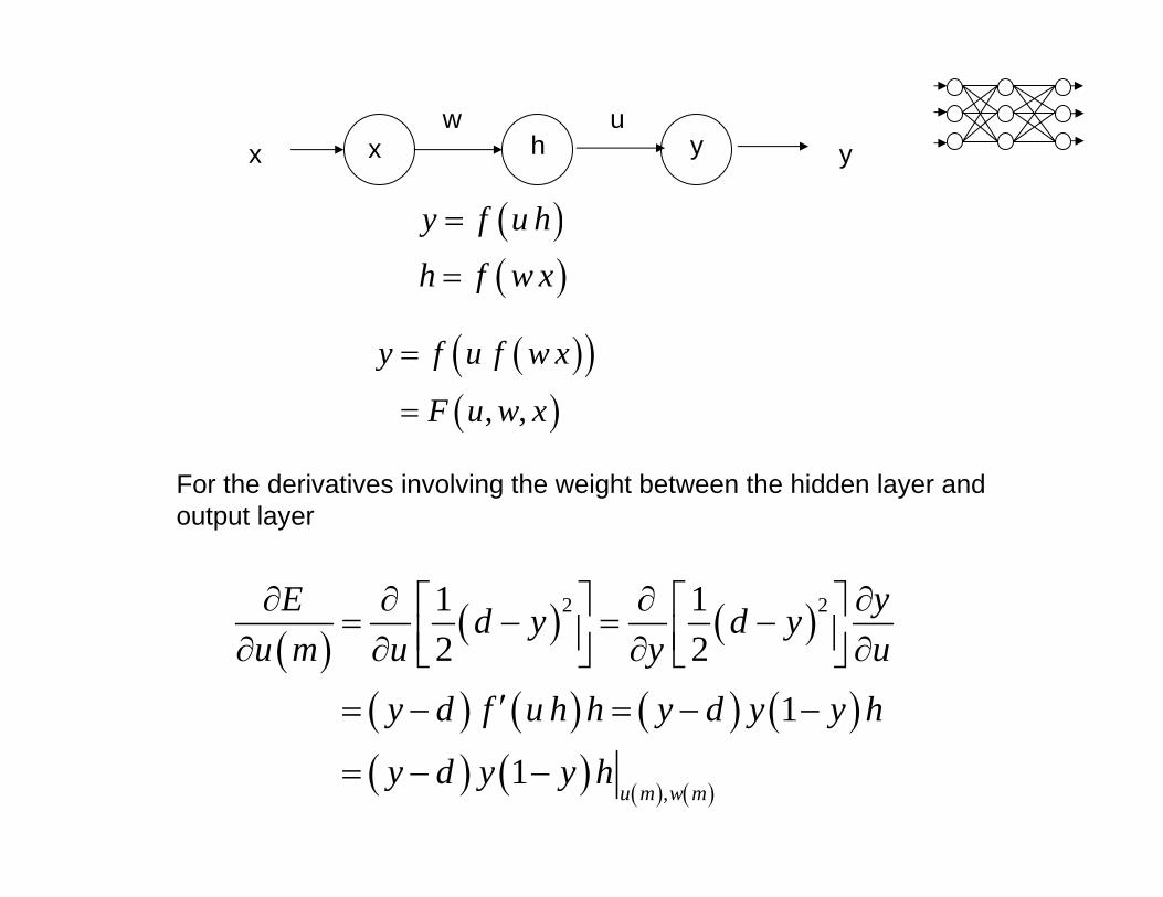
For the derivatives involving the weight between the hidden layer and output layer

( ) ( ) ( )

( ) ( ) ( ) ( ) ( ) ( )

( ) ( ) ( ) ( ) ( )

2 2

,

1 12 2

1

1 1u m w m

E yd y d yw m w y w

u hy d f u h y d y y u h w x x

wy d y y h h ux

∂ ∂ ∂ ∂⎡ ⎤ ⎡ ⎤= − = −⎢ ⎥ ⎢ ⎥∂ ∂ ∂ ∂⎣ ⎦ ⎣ ⎦

∂′ ′= − = − −

∂= − − −

Similarly for the weight between the hidden layer and input layer

Thus, the training algorithm is:

1. Initialize weights to small random values2. Using a training set of known pairs of inputs and outputs (x, d) change the weights according to

( ) ( ) ( ) ( ) ( ) ( ) ( )

( ) ( ) ( ) ( ) ( ) ( )

,

,

1 1 1

1 1u m w m

u m w m

w m w m y d y y h h u x

u m u m y d y y h

μ

μ

+ = − − − −

+ = − − −

with ( )( )

y f u h

h f w x

=

=until ( )21

2E d y= − becomes sufficiently small

E

stop

iteration

This is an example of supervised learning

hidden layer

outputs

One of the most popular neural nets is a feed forward net with one hidden layer trained by the back propagation algorithm

It can be shown that in principle this type of network can represent an arbitrary input-output mapping or solve an arbitraryclassification problem

Back propagation algorithm (three layer feed forward network)

jiw kjuP inputnodes

M hiddennodes

K outputnodes

( ) ( ) ( )

( ) ( ) ( ) ( )1

1 1,..., 1,...,

1 1 1,..., 1,...,

new oldkj kj k k k k j

Knew old oldji ji k k k k kj j j i

k

u u y d y y h k K j M

w w y d y y u h h x j M i P

μ

μ=

= − − − = =

= − − − − = =∑

1

1

1

1 exp

1

1 exp

k Moldkj j

j

j Poldji i

i

yu h

hw x

=

=

=⎛ ⎞

+ −⎜ ⎟⎝ ⎠

=⎛ ⎞

+ −⎜ ⎟⎝ ⎠

∑

∑

with

ykxi

Some issues associated with this "backprop" network

1. design of training, testing and validation data sets2. determination of the network structure3. selection of the learning rate (μ)4. problems with under or over-training

E

iterations

training set

testing set

stoplearning

overtrained

Some important issues for neural networks:

Pre-processing the data to provide:

• reduction of data dimensionality• noise filtering or suppression• enhancement

strengthening of relevant featurescentering data within a sensory aperture or windowscanning a window over the data

•invariance in the measurement space to:translationsrotationsscale changesdistortion

• data preparationanalog to digital conversiondata scalingdata normalizationthresholding

Some examples of pre-processing include

1-D and 2-D FFTsFilteringConvolution KernelsCorrelation Masks or Template MatchingAutocorrelationEdge Detection and EnhancementMorphological Image ProcessingFourier DescriptorsWalsh, Hadamard, Cosine, Hartley, Hotelling, Hough TransformsHigher order spectraHomomorphic Transformations (e.g. Cepstrums)Time-Frequency transforms ( Wavelet, Wigner-Ville, Zak)Linear Predictive CodingPrincipal Component AnalysisIndependent Component AnalysisGeometric MomentsThresholdingData SamplingScanning

Probabilistic Neural Network (PNN)

Basic idea:Use training samples themselves to obtain a representation of the probability distributions for each class and then use Bayes decision rule to make a classification

Basis functions usually chosen are Gaussians:

( )( )

( ) ( )/ 2 2

1

1 exp22

iT

Mij ij

i p pji

fM σπ σ =

⎡ ⎤− − −⎢ ⎥=⎢ ⎥⎣ ⎦

∑x x x x

x

i … class number (i = 1, 2, …, N)j … training pattern numberxij … j th training pattern from i th classMi … number of training vectors in class ip .. dimension of vector xfi (x) = sum of Gaussians centered at each training pattern from the ithclass to represent the probability density of that classσ … smoothing factor (standard deviation, width of the Gaussians)

probability density function for class i

ijx

If we normalize the vectors x and xij to unit length and assume the number of training samples from each class are in proportion to their a priori probability of occurrence then we can take as our decision function

( ) ( )( )

( )/ 2 2

1

11 exp2

iMij

i i i p pj

g M fσπ σ =

⎡ ⎤⋅ −= = ⎢ ⎥

⎢ ⎥⎣ ⎦∑

x xx x

( ) ( )( )

( )/ 2 2

1

11 exp2

iMij

i i i p pj

g M fσπ σ =

⎡ ⎤⋅ −= = ⎢ ⎥

⎢ ⎥⎣ ⎦∑

x xx x

Since we decide for a given class k based on

( ) ( )k ig g>x x for all ( )1,2,...,i N i k= ≠

the common constant outside the sum makes no difference and we can take

( ) ( )2

1

1exp

iMij

ij

gσ=

⎡ ⎤⋅ −= ⎢ ⎥

⎢ ⎥⎣ ⎦∑

x xx

This can now be easily implemented in a neural network form

x1 xj xp

1 M11 1Mi MN

∑ ∑ ∑

( )1g x ( )ig x ( )Ng x

Probabilistic Neural Network

weights arejust elements of the trainingpatternsxij

Characteristics of the PNN

1. no training, weights are just the training vectors themselves

2. only parameter that needs to be found is the smoothing factor, σ

3. outputs are representative of probabilities of each class directly

4. the decision surfaces are guaranteed to approach the Bayes optimal boundaries as the number of training samples grows

5. "outliers" are tolerated

6. sparse samples are adequate for good network performance

7. can update the network as new training samples become available

8. needs to store all the training samples, requiring a large memory

9. testing can be slower than with other nets

References

Specht, D.F., " Probabilistic neural networks," Neural Networks, 3, 109-118, 1990.

Zaknich, A., Neural Networks for Intelligent Signal Processing, World Scientific, 2003.

Haykin, S., Neural Networks, a Comprehensive Foundation, 2nd Ed., Prentice-Hall, 1999.

Bishop, C.S., Neural Networks for Pattern Recognition, Clarendon Press, 1995.

Resources

There are many, many neural network resources and tools available on the web.

Some software packages:

MATLAB Neural Network Toolbox www.mathworks.comNeuroshell Classifier www.wardsystems.comClassifierXL www.analyzerxl.comBrainmaker www.calsci.comNeurosolutions www.nd.comNeuroxl www.neuroxl.com