Neural Dynamic Policiesfor End-to-End Sensorimotor Learning

Shikhar BahlCMU

Mustafa MukadamFAIR

Abhinav GuptaCMU

Deepak PathakCMU

Abstract

The current dominant paradigm in sensorimotor control, whether imitation orreinforcement learning, is to train policies directly in raw action spaces suchas torque, joint angle, or end-effector position. This forces the agent to makedecisions individually at each timestep in training, and hence, limits the scalabilityto continuous, high-dimensional, and long-horizon tasks. In contrast, research inclassical robotics has, for a long time, exploited dynamical systems as a policyrepresentation to learn robot behaviors via demonstrations. These techniques,however, lack the flexibility and generalizability provided by deep learning orreinforcement learning and have remained under-explored in such settings. In thiswork, we begin to close this gap and embed the structure of a dynamical systeminto deep neural network-based policies by reparameterizing action spaces viasecond-order differential equations. We propose Neural Dynamic Policies (NDPs)that make predictions in trajectory distribution space as opposed to prior policylearning methods where actions represent the raw control space. The embeddedstructure allows end-to-end policy learning for both reinforcement and imitationlearning setups. We show that NDPs outperform the prior state-of-the-art in termsof either efficiency or performance across several robotic control tasks for bothimitation and reinforcement learning setups. Project video and code are availableat: https://shikharbahl.github.io/neural-dynamic-policies/.

1 Introduction

yif tn t

Tf tin itar frtT f It

TT f

Vanilla Policy NDP (Ours)

Figure 1: Vector field induced by NDPs. The goalis to draw the planar digit 4 from the start position.The dynamical structure in NDP induces a smoothvector field in trajectory space. In contrast, a vanillapolicy has to reason individually in different parts.

Consider an embodied agent tasked with throwinga ball into a bin. Not only does the agent need todecide where and when to release the ball, but alsoneeds to reason about the whole trajectory that itshould take such that the ball is imparted with thecorrect momentum to reach the bin. This form ofreasoning is necessary to perform many such ev-eryday tasks. Common methods in deep learningfor robotics tackle this problem either via imitationor reinforcement learning. However, in most cases,the agent’s policy is trained in raw action spaceslike torques, joint angles, or end-effector positions,which forces the agent to make decisions at eachtime step of the trajectory instead of making deci-sions in the trajectory space itself (see Figure 1). Butthen how do we reason about trajectories as actions?

A good trajectory parameterization is one that is able to capture a large set of an agent’s behaviorsor motions while being physically plausible. In fact, a similar question is also faced by scientists

34th Conference on Neural Information Processing Systems (NeurIPS 2020), Vancouver, Canada.

arX

iv:2

012.

0278

8v1

[cs

.LG

] 4

Dec

202

0

Forward Integrator

!!!!

fθΦ !t

Neural Dynamic Policy

(g, wi )

rt+k , st+k

Environment

at

st at+1

at+k

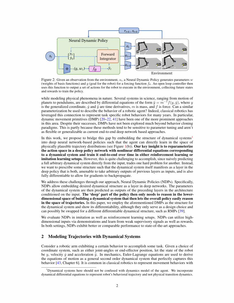
Figure 2: Given an observation from the environment, st, a Neural Dynamic Policy generates parameters w(weights of basis functions) and g (goal for the robot) for a forcing function fθ . An open loop controller thenuses this function to output a set of actions for the robot to execute in the environment, collecting future statesand rewards to train the policy.

while modeling physical phenomena in nature. Several systems in science, ranging from motion ofplanets to pendulums, are described by differential equations of the form y = m−1f(y, y), where yis the generalized coordinate, y and y are time derivatives, m is mass, and f is force. Can a similarparameterization be used to describe the behavior of a robotic agent? Indeed, classical robotics hasleveraged this connection to represent task specific robot behaviors for many years. In particular,dynamic movement primitives (DMP) [20–22, 41] have been one of the more prominent approachesin this area. Despite their successes, DMPs have not been explored much beyond behavior cloningparadigms. This is partly because these methods tend to be sensitive to parameter tuning and aren’tas flexible or generalizable as current end-to-end deep network based approaches.

In this work, we propose to bridge this gap by embedding the structure of dynamical systems1

into deep neural network-based policies such that the agent can directly learn in the space ofphysically plausible trajectory distributions (see Figure 1(b)). Our key insight is to reparameterizethe action space in a deep policy network with nonlinear differential equations correspondingto a dynamical system and train it end-to-end over time in either reinforcement learning orimitation learning setups. However, this is quite challenging to accomplish, since naively predictinga full arbitrary dynamical system directly from the input, trades one hard problem for another. Instead,we want to prescribe some structure such that the dynamical system itself manifests as a layer in thedeep policy that is both, amenable to take arbitrary outputs of previous layers as inputs, and is alsofully differentiable to allow for gradients to backpropagate.

We address these challenges through our approach, Neural Dynamic Policies (NDPs). Specifically,NDPs allow embedding desired dynamical structure as a layer in deep networks. The parametersof the dynamical system are then predicted as outputs of the preceding layers in the architectureconditioned on the input. The ‘deep’ part of the policy then only needs to reason in the lower-dimensional space of building a dynamical system that then lets the overall policy easily reasonin the space of trajectories. In this paper, we employ the aforementioned DMPs as the structure forthe dynamical system and show its differentiability, although they only serve as a design choice andcan possibly be swapped for a different differentiable dynamical structure, such as RMPs [39].

We evaluate NDPs in imitation as well as reinforcement learning setups. NDPs can utilize high-dimensional inputs via demonstrations and learn from weak supervisory signals as well as rewards.In both settings, NDPs exhibit better or comparable performance to state-of-the-art approaches.

2 Modeling Trajectories with Dynamical Systems

Consider a robotic arm exhibiting a certain behavior to accomplish some task. Given a choice ofcoordinate system, such as either joint-angles or end-effector position, let the state of the robotbe y, velocity y and acceleration y. In mechanics, Euler-Lagrange equations are used to derivethe equations of motion as a general second order dynamical system that perfectly captures thisbehavior [43, Chapter 6]. It is common in classical robotics to represent movement behaviors with

1Dynamical systems here should not be confused with dynamics model of the agent. We incorporatedynamical differential equations to represent robot’s behavioral trajectory and not physical transition dynamics.

2

such a dynamical system. Specifically, we follow the second order differential equation structureimposed by Dynamic Movement Primitives [22, 31, 41]. Given a desired goal state g, the behavior isrepresented as:

y = α(β(g − y)− y) + f(x), (1)where α, β are global parameters that allow critical damping of the system and smooth convergenceto the goal state. f is a non-linear forcing function which captures the shape of trajectory and operatesover x which serves to replace time dependency across trajectories, giving us the ability to modeltime invariant tasks, e.g., rhythmic motions. x evolves through the first-order linear system:

x = −axx (2)

The specifics of f are usually design choices. We use a sum of weighted Gaussian radial basisfunctions [22] shown below:

f(x, g) =

∑ψiwi∑ψi

x(g − y0), ψi = e(−hi(x−ci)2) (3)

where i indexes over n which is the number of basis functions. Coefficients ci = e−iαxn are the

horizontal shifts of each basis function, and hi = nci

are the width of each of each basis function. Theweights on each of the basis functions wi parameterize the forcing function f . This set of nonlineardifferential equations induces a smooth trajectory distribution that acts as an attractor towards adesired goal (see Figure 1, right). We now discuss how to combine this dynamical structure with deepneural network based policies in an end-to-end differentiable manner.

3 Neural Dynamic Policies (NDPs)

We condense actions into a space of trajectories, parameterized by a dynamical system, while keepingall the advantages of a deep learning based setup. We present a type of policy network, calledNeural Dynamic Policies (NDPs) that given an input, image or state, can produce parameters foran embedded dynamical structure, which reasons in trajectory space but outputs raw actions to beexecuted. Let the unstructured input to robot be s, (an image or any other sensory input), and theaction executed by the robot be a. We describe how we can incorporate a dynamical system as adifferentiable layer in the policy network, and how NDPs can be utilized to learn complex agentbehaviors in both imitation and reinforcement learning settings.

3.1 Neural Network Layer Parameterized by a Dynamical System

Throughout this paper, we employ the dynamical system described by the second order DMPequation (1). There are two key parameters that define what behavior will be described by thedynamical system presented in Section 2: basis function weights w = w1, . . . , wi, . . . , wn andgoal g. NDPs employ a neural network Φ which takes an unstructured input s2 and predicts theparameters w, g of the dynamical system. These predicted w, g are then used to solve the secondorder differential equation (1) to obtain system states y, y, y. Depending on the difference betweenthe choice of robot’s coordinate system for y and desired action a, we may need an inverse controllerΩ(.) to convert y to a, i.e., a = Ω(y, y, y). For instance, if y is in joint angle space and a is a torque,then Ω(.) is the robot’s inverse dynamics controller, and if y and a both are in joint angle space thenΩ(.) is the identity function.

As summarized in Figure 2, neural dynamic policies are defined as π(a|s; θ) , Ω(DE(Φ(s; θ)

))where DE(w, g) → y, y, y denotes solution of the differential equation (1). The forward pass ofπ(a|s) involves solving the dynamical system and backpropagation requires it to be differentiable.We now show how we differentiate through the dynamical system to train the parameters θ of NDPs.

3.2 Training NDPs by Differentiating through the Dynamical System

To train NDPs, estimated policy gradients must flow from a, through the parameters of the dynamicalsystem w and g, to the network Φ(s; θ). At any time t, given the previous state of robot yt−1 and

2robot’s state y is not to be confused with environment observation s which contains world as well as robotstate (and often velocity). s could be given by either an image or true state of the environment.

3

velocity yt−1 the output of the DMP in Equation (1) is given by the acceleration

yt = α(β(g − yt−1)− yt−1 + f(xt, g) (4)

Through Euler integration, we can find the next velocity and position after a small time interval dt

yt = yt−1 + yt−1dt, yt = yt−1 + yt−1dt (5)

In practice, this integration is implemented in m discrete steps. To perform a forward pass, we unrollthe integrator for m iterations starting from initial y0, y0. We can either apply all the m intermediaterobot states y as actions on the robot using inverse controller Ω(.), or equally sub-sample them intok ∈ 1,m actions in between, where k is the NDP rollout length. This frequency of samplingcould allow robot operation at a much higher frequency (.5-5KHz) than the environment (usually100Hz). The sampling frequency need not be same at training and inference as discussed further inSection 3.5.

Now we can compute gradients of the trajectory from the DMP with respect to w and g usingEquations (3)-(5) as follows:

∂f(xt, g)

∂wi=

ψi∑j ψj

(g − y0)xt,∂f(xt, g)

∂g=

ψjwj∑j ψj

xt (6)

Using this, a recursive relationship follows between, (similarly to the one derived by Pahic et al. [29])∂yt∂wi

, ∂yt∂g and the preceding derivatives of wi, g with respect to yt−1, yt−2, yt−1 and yt−2. Completederivation of equation (6) is given in appendix.

We now discuss how NDPs can be leveraged to train policies for imitation learning and reinforcementlearning setups.

3.3 Training NDPs for Imitation (Supervised) Learning

Training NDPs in imitation learning setup is rather straightforward. Given a sequence of inputs, s′, . . . , NDP’s π(s; θ) outputs a sequence of actions a, a′ . . .. In our experiments, s is a highdimensional image input. Let the demonstrated action sequence be τtarget, we just take a loss betweenthe predicted sequence as follows:

Limitation =∑s

||π(s)− τtarget(s)||2 (7)

The gradients of this loss are backpropagated as described in Section 3.2 to train the parameters θ.

3.4 Training NDPs for Reinforcement LearningAlgorithm 1 Training NDPs for RLRequire: Policy π, k NDP rollout length, Ω low-

level inverse controllerfor 1, 2, ... episodes do

for t = 0, k, . . . , until end of episode dow, g = Φ(st)Robot yt, yt from st (pos, vel)for m = 1, ...,M (integration steps) do

Estimate xm via (2) and update xmEstimate yt+m, yt+m, yt+m via (4), (5)a = Ω(yt+m, yt+m−1)Apply action a to get s′

Store transition (s, a, s′, r)end forCompute Policy gradient∇θJθ ← θ + η∇θJ

end forend for

We now show how an NDP can be used as a policy, π inthe RL setting. As discussed in Section 3.2, NDP sam-ples k actions for the agent to execute in the environmentgiven input observation s. One could use any underlyingRL algorithm to optimize the expected future returns. Inthis paper, we use Proximal Policy Optimization (PPO)[42] and treat a independently when computing the policygradient for each step of the NDP rollout and backpropvia a reinforce objective.

There are two choices for value function critic V π(s): ei-ther predict a single common value function for all theactions in the k-step rollout or predict different critic val-ues for each step in the NDP rollout sequence. We foundthat the latter works better in practice. We call this a multi-action critic architecture and predict k different estimatesof value using k-heads on top of the critic network. Later,in the experiments we perform ablations over the choice of k. To further create a strong baselinecomparison, as we discuss in Section 4, we also design and compare against a variant of PPO thatpredicts multiple actions using our multi-action critic architecture.

4

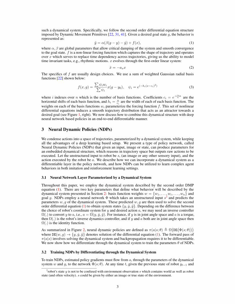
(a) Throwing (b) Picking (c) Pushing (d) Faucet Open (e) Soccer (f) 50 TasksFigure 3: Environment snapshot for different tasks considered in experiments. (a,b) Throwing and Pickingtasks are adapted from [17] on the Kinova Jaco arm. (c-f) Remaining tasks are adapted from Yu et al. [50].

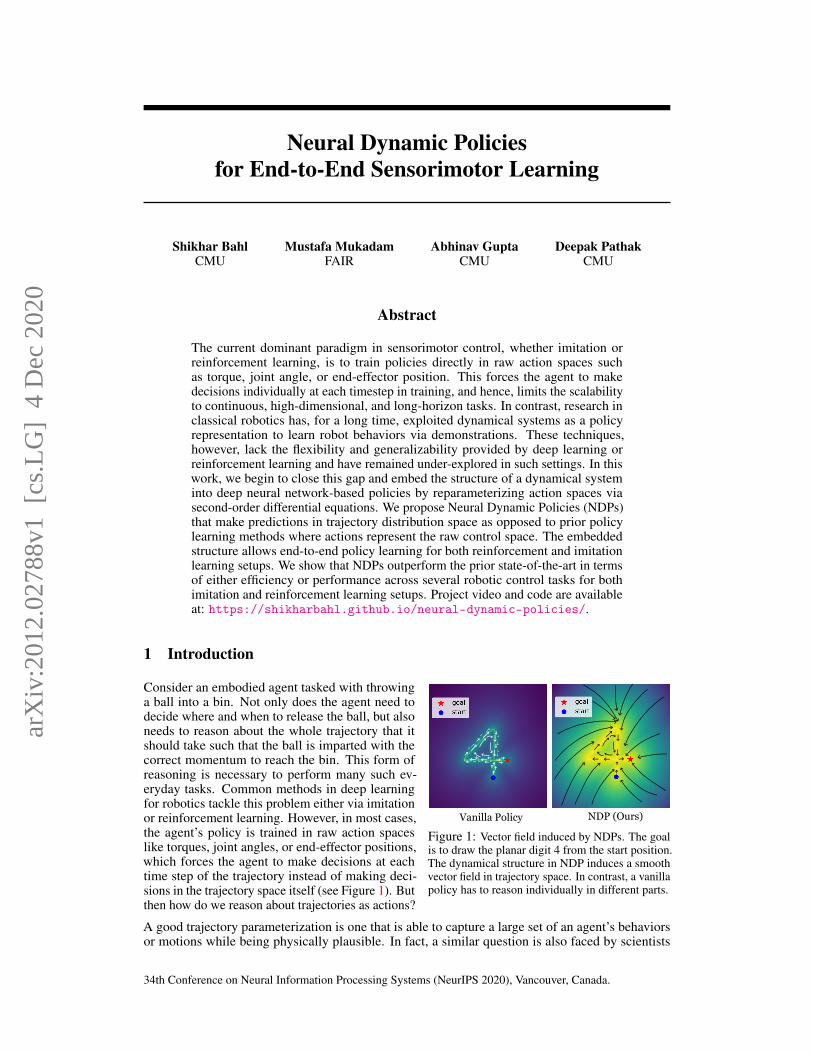
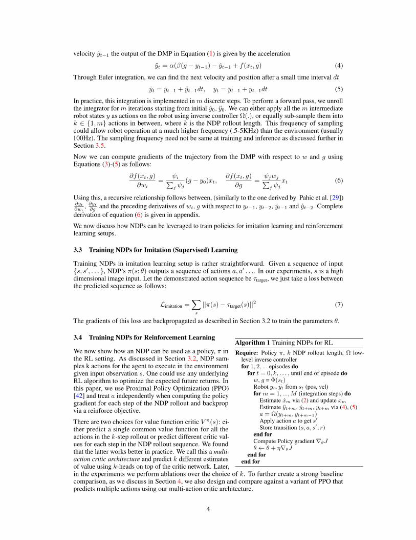
Input Ours CNN CNN-DMP Input Ours CNN CNN-DMPFigure 4: Imitation (supervised) learning results on held-out test images of the digit writing task. Given an inputimage (left), the output action is the end-effector position of a planar robot. All methods have the same neuralnetwork architecture for fair comparison. We find that the trajectories predicted by NDPs (ours) are dynamicallysmooth as well as more accurate than both baselines (a vanilla CNN and the architecture from Pahic et al. [29].

Algorithm 1 provides a summary of our method for training NDPs with policy gradients. We onlyshow results of using NDPs with on-policy RL (PPO), however, NDPs can similarly be adapted tooff-policy methods.

3.5 Inference in NDPs

In the case of inference, our method uses the NDP policy π once every k environment steps,hence requires k-times fewer forward passes as actions applied to the robot. While reducing theinference time in simulated tasks may not show much difference, in real world settings, wherelarge perception systems are usually involved, reducing inference time can help decrease overalltime costs. Additionally, deployed real world systems may not have the same computational poweras many systems used to train state-of-the-art RL methods on simulators, so inference costs endup accumulating, thus a method that does inference efficiently can be beneficial. Furthermore, asdiscussed in Section 3.2, the rollout length of NDP can be more densely sampled at test-time than attraining allowing the robot to produce smooth and dynamically stable motions. Compared to about100Hz frequency of the simulation, our method can make decisions an order of magnitude faster (atabout 0.5-5KHz) at inference.

4 Experimental Setup

Environments To test our method on dynamic environments, we took existing torque control basedenvironments for Picking and Throwing [17] and modified them to enable joint angle control. Therobot is a 6-DoF Kinova Jaco Arm. In Throwing, the robot tosses a cube into a bin, and in Picking,the robot picks up a cube and lifts it as high as possible. To test on quasi-static tasks, we use Pushing,Soccer, Faucet-Opening from the Meta-World [50] task suite, as well as a setup that requires learningall 50 tasks (MT50) jointly (see Figure 3). These Meta-World environments are all in end-effectorposition control settings and based on a Sawyer Robot simulation in Mujoco [47]. In order to makethe tasks more realistic, all environments have some degree of randomization. Picking and Throwinghave random starting positions, while the rest have randomized goals.

Baselines We use PPO [42] as the underlying optimization algorithm for NDPs and all the otherbaselines compared in the reinforcement learning setup. The first baseline is the PPO algorithmitself without the embedded dynamical structure. Further, as mentioned in the Section 3.2, NDPis able to operate the robot at a much higher frequency than the world. Precisely, its frequencyis k-times higher where k is the NDP rollout length (described in Section 3.2). Even though therobot moves at a higher frequency, the environment/world state is only observed at normal rate, i.e.,once every k robot steps and the reward computation at the intermediate k steps only uses the staleenvironment/world state from the first one of the k-steps. Hence, to create a stronger baseline that canalso operate at higher frequency, we create a “PPO-multi” baseline that predicts multiple actions and

5

also uses our multi-action critic architecture as described in Section 3.4. All methods are comparedin terms of performance measured against the environment sample states observed by the agent. Inaddition, we also compare to Variable Impedance Control in End-Effector Space (VICES) [26] andDynamics-Aware Embeddings (Dyn-E) [49] . VICES learns to output parameters of a PD controlleror an Impedance controller directly. Dyn-E, on the other hand, using forward prediction based onenvironment dynamics, learns a lower dimensional action embedding.

5 Evaluation Results: NDPs for Imitation and Reinforcement Learning

We validate our approach on Imitation Learning and RL tasks in order to ascertain how NDP comparesto state-of-the-art methods. We investigate: a) Does dynamical structure in NDPs help in learningfrom demonstrations in imitation learning setups?; b) How well do NDPs perform on dynamic andquasi-static tasks in deep reinforcement learning setups compared to the baselines?; c) How sensitiveis the performance of NDPs to different hyper-parameter settings?

5.1 Imitation (Supervised) Learning

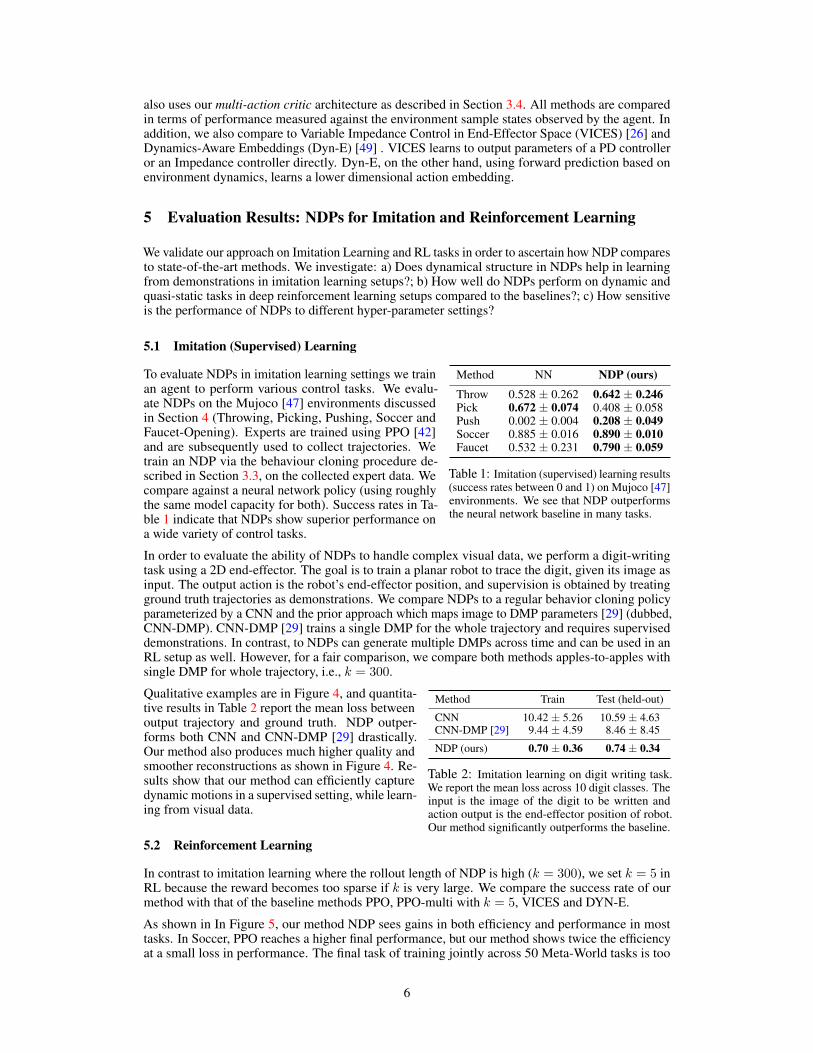
Method NN NDP (ours)Throw 0.528 ± 0.262 0.642 ± 0.246Pick 0.672 ± 0.074 0.408 ± 0.058Push 0.002 ± 0.004 0.208 ± 0.049Soccer 0.885 ± 0.016 0.890 ± 0.010Faucet 0.532 ± 0.231 0.790 ± 0.059

Table 1: Imitation (supervised) learning results(success rates between 0 and 1) on Mujoco [47]environments. We see that NDP outperformsthe neural network baseline in many tasks.

To evaluate NDPs in imitation learning settings we trainan agent to perform various control tasks. We evalu-ate NDPs on the Mujoco [47] environments discussedin Section 4 (Throwing, Picking, Pushing, Soccer andFaucet-Opening). Experts are trained using PPO [42]and are subsequently used to collect trajectories. Wetrain an NDP via the behaviour cloning procedure de-scribed in Section 3.3, on the collected expert data. Wecompare against a neural network policy (using roughlythe same model capacity for both). Success rates in Ta-ble 1 indicate that NDPs show superior performance ona wide variety of control tasks.

In order to evaluate the ability of NDPs to handle complex visual data, we perform a digit-writingtask using a 2D end-effector. The goal is to train a planar robot to trace the digit, given its image asinput. The output action is the robot’s end-effector position, and supervision is obtained by treatingground truth trajectories as demonstrations. We compare NDPs to a regular behavior cloning policyparameterized by a CNN and the prior approach which maps image to DMP parameters [29] (dubbed,CNN-DMP). CNN-DMP [29] trains a single DMP for the whole trajectory and requires superviseddemonstrations. In contrast, to NDPs can generate multiple DMPs across time and can be used in anRL setup as well. However, for a fair comparison, we compare both methods apples-to-apples withsingle DMP for whole trajectory, i.e., k = 300.

Method Train Test (held-out)

CNN 10.42 ± 5.26 10.59 ± 4.63CNN-DMP [29] 9.44 ± 4.59 8.46 ± 8.45

NDP (ours) 0.70 ± 0.36 0.74 ± 0.34

Table 2: Imitation learning on digit writing task.We report the mean loss across 10 digit classes. Theinput is the image of the digit to be written andaction output is the end-effector position of robot.Our method significantly outperforms the baseline.

Qualitative examples are in Figure 4, and quantita-tive results in Table 2 report the mean loss betweenoutput trajectory and ground truth. NDP outper-forms both CNN and CNN-DMP [29] drastically.Our method also produces much higher quality andsmoother reconstructions as shown in Figure 4. Re-sults show that our method can efficiently capturedynamic motions in a supervised setting, while learn-ing from visual data.

5.2 Reinforcement Learning

In contrast to imitation learning where the rollout length of NDP is high (k = 300), we set k = 5 inRL because the reward becomes too sparse if k is very large. We compare the success rate of ourmethod with that of the baseline methods PPO, PPO-multi with k = 5, VICES and DYN-E.

As shown in In Figure 5, our method NDP sees gains in both efficiency and performance in mosttasks. In Soccer, PPO reaches a higher final performance, but our method shows twice the efficiencyat a small loss in performance. The final task of training jointly across 50 Meta-World tasks is too

6

0.0 0.5 1.0 1.5 2.0Environment Samples 1e5

0.00.10.20.30.40.50.6

Succ

ess R

ate

ppodynEvicesppo-multiours

(a) Throwing

0 1 2 3 4 5Environment Samples 1e5

0.0

0.1

0.2

0.3

0.4

0.5

Succ

ess R

ate

(b) Picking

0.0 0.5 1.0 1.5 2.0 2.5 3.0Environment Samples 1e5

0.00.10.20.30.40.50.6

Succ

ess R

ate

(c) Pushing

0.0 0.5 1.0 1.5 2.0 2.5 3.0 3.5Environment Samples 1e5

0.0

0.2

0.4

0.6

0.8

Succ

ess R

ate

(d) Faucet Open

0 1 2 3 4 5Environment Samples 1e5

0.0

0.2

0.4

0.6

0.8

Succ

ess R

ate

(e) Soccer

0.0 0.2 0.4 0.6 0.8Environment Samples 1e6

0.000.020.040.060.080.100.12

Succ

ess R

ate

(f) Joint 50 MetaWorld Tasks

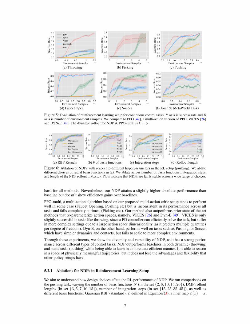
Figure 5: Evaluation of reinforcement learning setup for continuous control tasks. Y axis is success rate and Xaxis is number of environment samples. We compare to PPO [42], a multi-action version of PPO, VICES [26]and DYN-E [49]. The dynamic rollout for NDP & PPO-multi is k = 5.

0.0 0.5 1.0 1.5 2.0 2.5 3.0EQvLrRQmeQt 6amSles 1e5

−0.2

0.0

0.2

0.4

0.6

6ucc

ess 5

ate

0ultLquaGrLcLLQearGaussLaQIQv. 4uaGrLcIQv. 0ultLquaGrLc

(a) RBF Kernels

0.0 0.5 1.0 1.5 2.0 2.5 3.0EnvirRnment 6amSles 1e5

0.0

0.2

0.4

0.6

6uccess 5ate

1 21 61 101 151 20

(b) # of basis functions

0.0 0.5 1.0 1.5 2.0 2.5 3.0EnvirRnment 6amSles 1e5

−0.2

0.0

0.2

0.4

0.6

6uccess 5ate

Int-steSs 15Int-steSs 25Int-steSs 35Int-steSs 45

(c) Integration steps

0.0 0.5 1.0 1.5 2.0 2.5 3.0EnvirRnment 6amSles 1e5

−0.10.00.10.20.30.40.50.6

6uccess 5ate

7 37 57 77 107 15

(d) Rollout length

Figure 6: Ablation of NDPs with respect to different hyperparameters in the RL setup (pushing). We ablatedifferent choices of radial basis functions in (a). We ablate across number of basis functions, integration steps,and length of the NDP rollout in (b,c,d). Plots indicate that NDPs are fairly stable across a wide range of choices.

hard for all methods. Nevertheless, our NDP attains a slightly higher absolute performance thanbaseline but doesn’t show efficiency gains over baselines.

PPO-multi, a multi-action algorithm based on our proposed multi-action critic setup tends to performwell in some case (Faucet Opening, Pushing etc) but is inconsistent in its performance across alltasks and fails completely at times, (Picking etc.). Our method also outperforms prior state-of-the-artmethods that re-paremeterize action spaces, namely, VICES [26] and Dyn-E [49]. VICES is onlyslightly successful in tasks like throwing, since a PD controller can efficiently solve the task, but sufferin more complex settings due to a large action space dimensionality (as it predicts multiple quantitiesper degree of freedom). Dyn-E, on the other hand, performs well on tasks such as Pushing, or Soccer,which have simpler dynamics and contacts, but fails to scale to more complex environments.

Through these experiments, we show the diversity and versatility of NDP, as it has a strong perfor-mance across different types of control tasks. NDP outperforms baselines in both dynamic (throwing)and static tasks (pushing) while being able to learn in a more data efficient manner. It is able to reasonin a space of physically meaningful trajectories, but it does not lose the advantages and flexibility thatother policy setups have.

5.2.1 Ablations for NDPs in Reinforcement Learning Setup

We aim to understand how design choices affect the RL performance of NDP. We run comparisons onthe pushing task, varying the number of basis functions N (in the set 2, 6, 10, 15, 20), DMP rolloutlengths (in set 3, 5, 7, 10, 15), number of integration steps (in set 15, 25, 35, 45), as well asdifferent basis functions: Gaussian RBF (standard), ψ defined in Equation (3), a liner map ψ(x) = x,

7

a multiquadric map: ψ(x) =√

1 + (εx)2, a inverse quadric map ψ(x) = 11+(εx)2 , and an inverse

multiquadric map: ψ(x) = 1√1+(εx)2

.

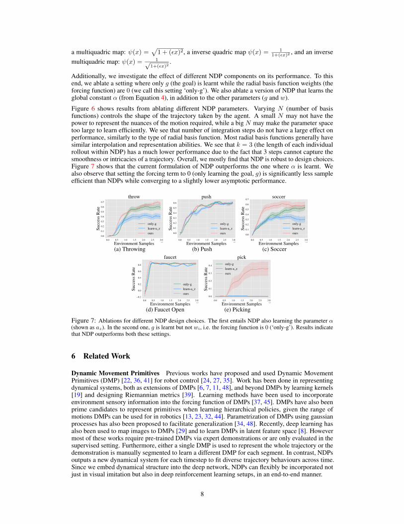
Additionally, we investigate the effect of different NDP components on its performance. To thisend, we ablate a setting where only g (the goal) is learnt while the radial basis function weights (theforcing function) are 0 (we call this setting ‘only-g’). We also ablate a version of NDP that learns theglobal constant α (from Equation 4), in addition to the other parameters (g and w).

Figure 6 shows results from ablating different NDP parameters. Varying N (number of basisfunctions) controls the shape of the trajectory taken by the agent. A small N may not have thepower to represent the nuances of the motion required, while a big N may make the parameter spacetoo large to learn efficiently. We see that number of integration steps do not have a large effect onperformance, similarly to the type of radial basis function. Most radial basis functions generally havesimilar interpolation and representation abilities. We see that k = 3 (the length of each individualrollout within NDP) has a much lower performance due to the fact that 3 steps cannot capture thesmoothness or intricacies of a trajectory. Overall, we mostly find that NDP is robust to design choices.Figure 7 shows that the current formulation of NDP outperforms the one where α is learnt. Wealso observe that setting the forcing term to 0 (only learning the goal, g) is significantly less sampleefficient than NDPs while converging to a slightly lower asymptotic performance.

0.0 0.5 1.0 1.5 2.0 2.5 3.0Environment Samples 1e5

0.0

0.1

0.2

0.3

0.4

0.5

0.6

0.7

Succ

ess R

ate

throw

only-glearn-a_zours

(a) Throwing

0.0 0.5 1.0 1.5 2.0 2.5 3.0Environment Samples 1e5

0.0

0.1

0.2

0.3

0.4

0.5

0.6

Succ

ess R

ate

push

only-glearn-a_zours

(b) Push

0.0 0.5 1.0 1.5 2.0 2.5 3.0Environment Samples 1e5

0.0

0.1

0.2

0.3

0.4

0.5

0.6

0.7

Succ

ess R

ate

soccer

only-glearn-a_zours

(c) Soccer

0.0 0.5 1.0 1.5 2.0 2.5 3.0Environment Samples 1e5

−0.2

0.0

0.2

0.4

0.6

0.8

Succ

ess R

ate

faucet

only-glearn-a_zours

(d) Faucet Open

0.0 0.5 1.0 1.5 2.0 2.5 3.0Environment Samples 1e5

0.0

0.1

0.2

0.3

0.4

Succ

ess R

ate

pickonly-glearn-a_zours

(e) Picking

Figure 7: Ablations for different NDP design choices. The first entails NDP also learning the parameter α(shown as az). In the second one, g is learnt but not wi, i.e. the forcing function is 0 (‘only-g’). Results indicatethat NDP outperforms both these settings.

6 Related Work

Dynamic Movement Primitives Previous works have proposed and used Dynamic MovementPrimitives (DMP) [22, 36, 41] for robot control [24, 27, 35]. Work has been done in representingdynamical systems, both as extensions of DMPs [6, 7, 11, 48], and beyond DMPs by learning kernels[19] and designing Riemannian metrics [39]. Learning methods have been used to incorporateenvironment sensory information into the forcing function of DMPs [37, 45]. DMPs have also beenprime candidates to represent primitives when learning hierarchical policies, given the range ofmotions DMPs can be used for in robotics [13, 23, 32, 44]. Parametrization of DMPs using gaussianprocesses has also been proposed to facilitate generalization [34, 48]. Recently, deep learning hasalso been used to map images to DMPs [29] and to learn DMPs in latent feature space [8]. Howevermost of these works require pre-trained DMPs via expert demonstrations or are only evaluated in thesupervised setting. Furthermore, either a single DMP is used to represent the whole trajectory or thedemonstration is manually segmented to learn a different DMP for each segment. In contrast, NDPsoutputs a new dynamical system for each timestep to fit diverse trajectory behaviours across time.Since we embed dynamical structure into the deep network, NDPs can flexibly be incorporated notjust in visual imitation but also in deep reinforcement learning setups, in an end-to-end manner.

8

Reparameterized Policy and Action Spaces A broader area of work that makes use of actionreparameterization is the study of Hierarchical Reinforcement Learning (HRL). Works in the optionsframework [4, 46] attempt to learn an overarching policy that controls usage of lower-level policies orprimitives. Lower-level policies are usually pre-trained therefore require supervision and knowledgeof the task beforehand, limiting the generalizability of such methods. For example, Daniel et al.[13], Parisi et al. [30] incorporate DMPs into option-based RL policies, using a pre-trained DMPs asthe high level actions. This setup requires re-learning DMPs for different types of tasks and doesnot allow the same policy to generalize, since it needs to have access to an extremely large numberof DMPs. Action spaces can also be reparameterized in terms of pre-determined PD controller [51]or learned impedance controller parameters [26]. While this helps for policies to adapt to contactrich behaviors, it does not change the trajectories taken by the robot. This often leads to highdimensionality, and thus a decrease sample efficiency. In addition, Whitney et al. [49] learn an actionembedding based on passive data, however, this does not take environment dynamics or explicitcontrol structure into account.

Structure in Policy Learning Various methods in the field of control and robotics have employedphysical knowledge, dynamical systems, optimization, and more general task/environment dynamicsto create structured learning. Works such as [12, 18] propose networks constrained through physicalproperties such as Hamiltonian co-ordinates or Lagrangian Dynamics. However, the scope of theseworks is limited to toy examples such as a point mass, and are often used for supervised learning.Similarly, other works [28, 33, 38, 40] all employ dynamical systems to model demonstrations, anddo not tackle generalization or learning beyond imitation. Fully differentiable optimization problemshave also been incorporated as layers inside a deep learning setup [1, 2, 9]. Whil they share theunderlying idea of embedding structure in deep networks such that some aspects of this structurecan be learned end-to-end, they have not been explored in tackling complex robotic control tasks.Furthermore, it is common in RL setups to incorporate planning based on a system model [3, 10, 14–16]. However, this is usually learned from experience or from attempts to predict the effects of actionson the environment (forward and inverse models), and often tends to fail for complex dynamic tasks.

7 Discussion

Our method attempts to bridge the gap between classical robotics, control and recent approachesin deep learning and deep RL. We propose a novel re-parameterization of action spaces via NeuralDynamic Policies, a set of policies which impose the structure of a dynamical system on actionspaces. We show how this set of policies can be useful for continuous control with RL, as well asin supervised learning settings. Our method obtains superior results due to its natural imposition ofstructure and yet it is still generalizable to almost any continuous control environment.

The use of DMPs in this work was a particular design choice within our architecture which allowsfor any form of dynamical structure that is differentiable. As alluded to in the introduction, othersimilar representations can be employed in their place. In fact, DMPs are a special case of a generalsecond order dynamical system [5, 39] where the inertia term is identity, and potential and dampingfunctions are defined in a particular manner via first order differential equations with a separateforcing function which captures the complexities of the desired behavior. Given this, one can setupa dynamical structure such that it explicitly models and learns the metric, potential, and dampingexplicitly. While this brings advantages in better representation, it also brings challenges in learning.We leave these directions for future work to explore.

Acknowledgments

We thank Giovanni Sutanto, Stas Tiomkin and Adithya Murali for fruitful discussions. We also thankFranziska Meier, Akshara Rai, David Held, Mengtian Li, George Cazenavette, and Wen-Hsuan Chufor comments on early drafts of this paper. This work was supported in part by DARPA MachineCommon Sense grant and Google Faculty Award to DP.

9

References

[1] B. Amos and J. Z. Kolter. Optnet: Differentiable optimization as a layer in neural networks. InICML, 2017. 9

[2] B. Amos, I. D. J. Rodriguez, J. Sacks, B. Boots, and J. Z. Kolter. Differentiable mpc forend-to-end planning and control. In NeurIPS, 2018. 9

[3] C. G. Atkeson and J. C. Santamaria. A comparison of direct and model-based reinforcementlearning. In ICRA, 1997. 9

[4] P.-L. Bacon, J. Harb, and D. Precup. The option-critic architecture. In AAAI, 2017. 9

[5] F. Bullo and A. D. Lewis. Geometric Control of Mechanical Systems. Springer, 2005. 9

[6] S. Calinon. A tutorial on task-parameterized movement learning and retrieval. IntelligentService Robotics, 2016. 8

[7] S. Calinon, I. Sardellitti, and D. G. Caldwell. Learning-based control strategy for safe human-robot interaction exploiting task and robot redundancies. IROS, 2010. 8

[8] N. Chen, M. Karl, and P. Van Der Smagt. Dynamic movement primitives in latent space oftime-dependent variational autoencoders. In International Conference on Humanoid Robots(Humanoids), 2016. 8

[9] T. Q. Chen, Y. Rubanova, J. Bettencourt, and D. K. Duvenaud. Neural ordinary differentialequations. In NeurIPS, 2018. 9

[10] K. Chua, R. Calandra, R. McAllister, and S. Levine. Deep reinforcement learning in a handfulof trials using probabilistic dynamics models. arXiv preprint arXiv:1805.12114, 2018. 9

[11] A. Conkey and T. Hermans. Active learning of probabilistic movement primitives. 2019IEEE-RAS 19th International Conference on Humanoid Robots (Humanoids), 2019. 8

[12] M. Cranmer, S. Greydanus, S. Hoyer, P. Battaglia, D. Spergel, and S. Ho. Lagrangian neuralnetworks. arXiv preprint arXiv:2003.04630, 2020. 9

[13] C. Daniel, G. Neumann, O. Kroemer, and J. Peters. Hierarchical relative entropy policy search.Journal of Machine Learning Research, 2016. 8, 9

[14] M. Deisenroth and C. E. Rasmussen. Pilco: A model-based and data-efficient approach topolicy search. In ICML, 2011. 9

[15] M. P. Deisenroth, G. Neumann, and J. Peters. A survey on policy search for robotics. Found.Trends Robot, 2013.

[16] M. P. Deisenroth, D. Fox, and C. E. Rasmussen. Gaussian processes for data-efficient learningin robotics and control. IEEE Transactions on Pattern Analysis and Machine Intelligence, 2015.9

[17] D. Ghosh, A. Singh, A. Rajeswaran, V. Kumar, and S. Levine. Divide-and-conquer reinforce-ment learning. arXiv preprint arXiv:1711.09874, 2017. 5, 15

[18] S. Greydanus, M. Dzamba, and J. Yosinski. Hamiltonian neural networks. In NeurIPS, 2019. 9

[19] Y. Huang, L. Rozo, J. Silvério, and D. G. Caldwell. Kernelized movement primitives. TheInternational Journal of Robotics Research, 2019. 8

[20] A. J. Ijspeert, J. Nakanishi, and S. Schaal. Movement imitation with nonlinear dynamicalsystems in humanoid robots. In ICRA. IEEE, 2002. 2

[21] A. J. Ijspeert, J. Nakanishi, and S. Schaal. Learning attractor landscapes for learning motorprimitives. In NeurIPS, 2003.

10

[22] A. J. Ijspeert, J. Nakanishi, H. Hoffmann, P. Pastor, and S. Schaal. Dynamical movementprimitives: Learning attractor models for motor behaviors. Neural Computation, 2013. 2, 3, 8

[23] J. Kober and J. Peters. Learning motor primitives for robotics. In ICRA, 2009. 8

[24] P. Kormushev, S. Calinon, and D. G. Caldwell. Robot motor skill coordination with em-basedreinforcement learning. In IROS, 2010. 8

[25] I. Kostrikov. Pytorch implementations of reinforcement learning algorithms. https://github.com/ikostrikov/pytorch-a2c-ppo-acktr-gail, 2018. 15, 16

[26] R. Martin-Martin, M. A. Lee, R. Gardner, S. Savarese, J. Bohg, and A. Garg. Variable impedancecontrol in end-effector space: An action space for reinforcement learning in contact-rich tasks.IROS, 2019. 6, 7, 9, 15, 16

[27] K. Mülling, J. Kober, O. Kroemer, and J. Peters. Learning to select and generalize strikingmovements in robot table tennis. The International Journal of Robotics Research, 2013. 8

[28] K. Neumann and J. Steil. Learning robot motions with stable dynamical systems under diffeo-morphic transformations. Robotics and Autonomous Systems, 2015. 9

[29] R. Pahic, A. Gams, A. Ude, and J. Morimoto. Deep encoder-decoder networks for mapping rawimages to dynamic movement primitives. ICRA, 2018. 4, 5, 6, 8

[30] S. Parisi, H. Abdulsamad, A. Paraschos, C. Daniel, and J. Peters. Reinforcement learning vshuman programming in tetherball robot games. In IROS, 2015. 9

[31] P. Pastor, H. Hoffmann, T. Asfour, and S. Schaal. Learning and generalization of motor skillsby learning from demonstration. In ICRA, 2009. 3

[32] P. Pastor, M. Kalakrishnan, S. Chitta, E. Theodorou, and S. Schaal. Skill learning and taskoutcome prediction for manipulation. In ICRA, 2011. 8

[33] N. Perrin and P. Schlehuber-Caissier. Fast diffeomorphic matching to learn globally asymptoti-cally stable nonlinear dynamical systems. Systems & Control Letters, 2016. 9

[34] A. Pervez and D. Lee. Learning task-parameterized dynamic movement primitives using mixtureof gmms. Intelligent Service Robotics, 2018. 8

[35] J. Peters, S. Vijayakumar, and S. Schaal. Reinforcement learning for humanoid robotics. InInternational Conference on Humanoid Robots, 2003. 8

[36] M. Prada, A. Remazeilles, A. Koene, and S. Endo. Dynamic movement primitives for human-robot interaction: Comparison with human behavioral observation. In International Conferenceon Intelligent Robots and Systems, 2013. 8

[37] A. Rai, G. Sutanto, S. Schaal, and F. Meier. Learning feedback terms for reactive planning andcontrol. In ICRA, 2017. 8

[38] M. A. Rana, A. Li, D. Fox, B. Boots, F. Ramos, and N. Ratliff. Euclideanizing flows: Diffeo-morphic reduction for learning stable dynamical systems. arXiv preprint arXiv:2005.13143,2020. 9

[39] N. D. Ratliff, J. Issac, D. Kappler, S. Birchfield, and D. Fox. Riemannian motion policies. arXivpreprint arXiv:1801.02854, 2018. 2, 8, 9

[40] H. Ravichandar, I. Salehi, and A. Dani. Learning partially contracting dynamical systems fromdemonstrations. In CoRL, 2017. 9

[41] S. Schaal. Dynamic movement primitives-a framework for motor control in humans andhumanoid robotics. In Adaptive motion of animals and machines. Springer, 2006. 2, 3, 8

[42] J. Schulman, F. Wolski, P. Dhariwal, A. Radford, and O. Klimov. Proximal policy optimizationalgorithms. arXiv:1707.06347, 2017. 4, 5, 6, 7, 15, 16

11

[43] M. W. Spong, S. Hutchinson, and M. Vidyasagar. Robot modeling and control. John Wiley &Sons, 2020. 2

[44] F. Stulp, E. A. Theodorou, and S. Schaal. Reinforcement learning with sequences of motionprimitives for robust manipulation. Transactions on Robotics, 2012. 8

[45] G. Sutanto, Z. Su, S. Schaal, and F. Meier. Learning sensor feedback models from demonstra-tions via phase-modulated neural networks. In ICRA, 2018. 8

[46] R. S. Sutton, D. Precup, and S. Singh. Between mdps and semi-mdps: A framework for temporalabstraction in reinforcement learning. Artificial Intelligence, 1999. 9

[47] E. Todorov, T. Erez, and Y. Tassa. MuJoCo: A physics engine for model-based control. In TheIEEE/RSJ International Conference on Intelligent Robots and Systems, 2012. 5, 6

[48] A. Ude, A. Gams, T. Asfour, and J. Morimoto. Task-specific generalization of discrete andperiodic dynamic movement primitives. Transactions on Robotics, 2010. 8

[49] W. Whitney, R. Agarwal, K. Cho, and A. Gupta. Dynamics-aware embeddings. arXiv preprintarXiv:1908.09357, 2019. 6, 7, 9, 15, 16

[50] T. Yu, D. Quillen, Z. He, R. Julian, K. Hausman, C. Finn, and S. Levine. Meta-world: Abenchmark and evaluation for multi-task and meta reinforcement learning. arXiv preprintarXiv:1910.10897, 2019. 5, 15

[51] Y. Yuan and K. Kitani. Ego-pose estimation and forecasting as real-time pd control. In ICCV,2019. 9

12

A Appendix

A.1 Videos

Videos can also be found at: https://shikharbahl.github.io/neural-dynamic-policies/.We found that NDP results look dynamically more stable and smooth in comparison to the baselines.PPO-multi generates shaky trajectories, while corresponding NDP (ours) trajectories are muchsmoother .This is perhaps due to the embedded dynamical structure in NDPs as all other aspects inPPO-multi and NDP (ours) are compared apples-to-apples.

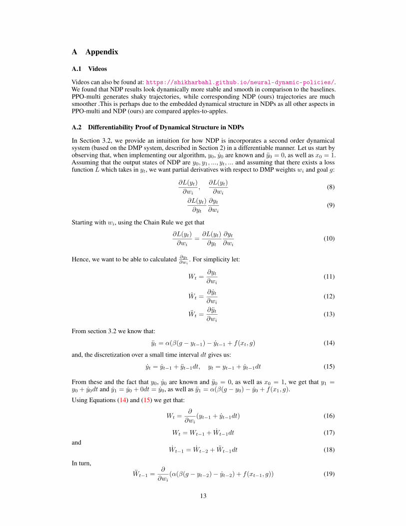
A.2 Differentiability Proof of Dynamical Structure in NDPs

In Section 3.2, we provide an intuition for how NDP is incorporates a second order dynamicalsystem (based on the DMP system, described in Section 2) in a differentiable manner. Let us start byobserving that, when implementing our algorithm, y0, y0 are known and y0 = 0, as well as x0 = 1.Assuming that the output states of NDP are y0, y1, ..., yt, ... and assuming that there exists a lossfunction L which takes in yt, we want partial derivatives with respect to DMP weights wi and goal g:

∂L(yt)

∂wi,

∂L(yt)

∂wi(8)

∂L(yt)

∂yt

∂yt∂wi

(9)

Starting with wi, using the Chain Rule we get that

∂L(yt)

∂wi=∂L(yt)

∂yt

∂yt∂wi

(10)

Hence, we want to be able to calculated ∂yt∂wi

. For simplicity let:

Wt =∂yt∂wi

(11)

Wt =∂yt∂wi

(12)

Wt =∂yt∂wi

(13)

From section 3.2 we know that:

yt = α(β(g − yt−1)− yt−1 + f(xt, g) (14)

and, the discretization over a small time interval dt gives us:

yt = yt−1 + yt−1dt, yt = yt−1 + yt−1dt (15)

From these and the fact that y0, y0 are known and y0 = 0, as well as x0 = 1, we get that y1 =y0 + y0dt and y1 = y0 + 0dt = y0, as well as y1 = α(β(g − y0)− y0 + f(x1, g).

Using Equations (14) and (15) we get that:

Wt =∂

∂wi(yt−1 + yt−1dt) (16)

Wt = Wt−1 + Wt−1dt (17)and

Wt−1 = Wt−2 + Wt−1dt (18)

In turn,

Wt−1 =∂

∂wi(α(β(g − yt−2)− yt−2) + f(xt−1, g)) (19)

13

From section 3.2, we know that∂f(xt−1, g)

∂wi=

ψi∑j ψj

(g − y0)xt−1 (20)

Hence:Wt−1 = α(β(−Wt−2)− Wt−2) +

ψi∑j ψj

(g − y0)xt−1 (21)

Plugging equations the value of Wt−1 into Equation (18):

Wt−1 = Wt−2 + (α(β(−Wt−2)− Wt−2) +ψi∑j ψj

(g − y0)xt−1)dt (22)

Now plugging the value of Wt−1 in Equation (17):

Wt = Wt−1 + (Wt−2 + (α(β(−Wt−2)− Wt−2) +ψi∑j ψj

(g − y0)xt−1)dt)dt (23)

We see that the value of Wt is dependent on Wt−1, Wt−2,Wt−2. We can now show that we can ac-quire a numerical value for Wt by recursively following the gradients, given that Wt−1, Wt−2,Wt−2are known. Since we showed that y0, y0, y1,y1 do not requirewi in their computation,W1, W0,W0 =0. Hence by recursively following the relationship defined in Equation (23), we achieve a solution forWt.

Similarly, let:

Gt =∂

∂g(yt−1 + yt−1dt) (24)

Gt = Gt−1 + Gt−1dt (25)and

Gt−1 = Gt−2 + Gt−1dt (26)

Using section 3.2, we get that∂f(xt−1, g)

∂g=

ψjwj∑j ψj

xt−1 (27)

Hence:Gt−1 = α(β(1−Gt−2)− Gt−2) +

ψjwj∑j ψj

xt−1 (28)

and we get a similar relationship as Equation (23):

Gt = Gt−1 + (Gt−2 + (α(β(1−Gt−2)− Gt−2) +ψjwj∑j ψj

xt−1)dt)dt (29)

Hence, Gt, similarly is dependent on Gt−1, Gt−2, Gt−2. We can use a similar argument as withwi to show that Gt is also numerically achievable. We have now shown that yt, the output of thedynamical system defined by a DMP, is differentiable with respect to wi and g.

A.3 Ablations

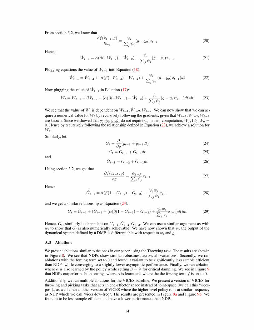
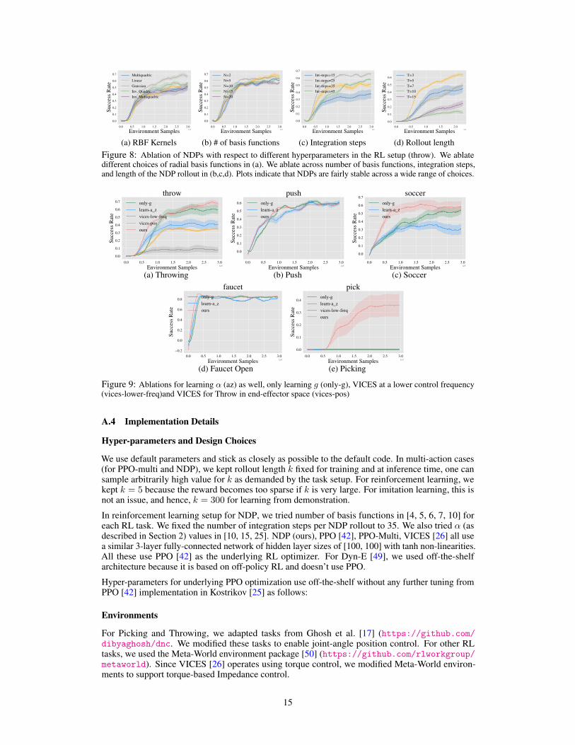
We present ablations similar to the ones in our paper, using the Throwing task. The results are showinin Figure 8. We see that NDPs show similar robustness across all variations. Secondly, we ranablations with the forcing term set to 0 and found it variant to be significantly less sample efficientthan NDPs while converging to a slightly lower asymptotic performance. Finally, we ran ablationwhere α is also learned by the policy while setting β = α

4 for critical damping. We see in Figure 9that NDPs outperforms both settings where α is learnt and where the the forcing term f is set to 0.

Additionally, we ran multiple ablations for the VICES baseline. We present a version of VICES forthrowing and picking tasks that acts in end-effector space instead of joint-space (we call this ‘vices-pos‘)., as well e ran another version of VICES where the higher level policy runs at similar frequencyas NDP which we call ‘vices-low-freq‘. The results are presented in Figure 9a and Figure 9b. Wefound it to be less sample efficient and have a lower performance than NDP.

14

0.0 0.5 1.0 1.5 2.0 2.5 3.0Environment Samples 1e5

0.0

0.1

0.2

0.3

0.4

0.5

0.6

0.7

Succ

ess R

ate

MultiquadricLinearGaussianInv. QuadricInv. Multiquadric

(a) RBF Kernels

0.0 0.5 1.0 1.5 2.0 2.5 3.0Environment Samples 1e5

0.0

0.1

0.2

0.3

0.4

0.5

0.6

0.7

Succ

ess R

ate

N=2N=5N=10N=15N=20

(b) # of basis functions

0.0 0.5 1.0 1.5 2.0 2.5 3.0Environment Samples 1e5

0.0

0.1

0.2

0.3

0.4

0.5

0.6

0.7

Succ

ess R

ate

Int-steps=15Int-steps=25Int-steps=35Int-steps=45

(c) Integration steps

0.0 0.5 1.0 1.5 2.0Environment Samples 1e5

0.0

0.1

0.2

0.3

0.4

0.5

0.6

Succ

ess R

ate

T=3T=5T=7T=10T=15

(d) Rollout lengthFigure 8: Ablation of NDPs with respect to different hyperparameters in the RL setup (throw). We ablatedifferent choices of radial basis functions in (a). We ablate across number of basis functions, integration steps,and length of the NDP rollout in (b,c,d). Plots indicate that NDPs are fairly stable across a wide range of choices.

0.0 0.5 1.0 1.5 2.0 2.5 3.0Environment Samples 1e5

0.0

0.1

0.2

0.3

0.4

0.5

0.6

0.7

Succ

ess R

ate

throwonly-glearn-a_zvices-low-freqvices-posours

(a) Throwing

0.0 0.5 1.0 1.5 2.0 2.5 3.0Environment Samples 1e5

0.0

0.1

0.2

0.3

0.4

0.5

0.6

Succ

ess R

ate

pushonly-glearn-a_zours

(b) Push

0.0 0.5 1.0 1.5 2.0 2.5 3.0Environment Samples 1e5

0.0

0.1

0.2

0.3

0.4

0.5

0.6

0.7

Succ

ess R

ate

socceronly-glearn-a_zours

(c) Soccer

0.0 0.5 1.0 1.5 2.0 2.5 3.0Environment Samples 1e5

−0.2

0.0

0.2

0.4

0.6

0.8

Succ

ess R

ate

faucetonly-glearn-a_zours

(d) Faucet Open

0.0 0.5 1.0 1.5 2.0 2.5 3.0Environment Samples 1e5

0.0

0.1

0.2

0.3

0.4

Succ

ess R

atepick

only-glearn-a_zvices-low-freqours

(e) Picking

Figure 9: Ablations for learning α (az) as well, only learning g (only-g), VICES at a lower control frequency(vices-lower-freq)and VICES for Throw in end-effector space (vices-pos)

A.4 Implementation Details

Hyper-parameters and Design Choices

We use default parameters and stick as closely as possible to the default code. In multi-action cases(for PPO-multi and NDP), we kept rollout length k fixed for training and at inference time, one cansample arbitrarily high value for k as demanded by the task setup. For reinforcement learning, wekept k = 5 because the reward becomes too sparse if k is very large. For imitation learning, this isnot an issue, and hence, k = 300 for learning from demonstration.

In reinforcement learning setup for NDP, we tried number of basis functions in [4, 5, 6, 7, 10] foreach RL task. We fixed the number of integration steps per NDP rollout to 35. We also tried α (asdescribed in Section 2) values in [10, 15, 25]. NDP (ours), PPO [42], PPO-Multi, VICES [26] all usea similar 3-layer fully-connected network of hidden layer sizes of [100, 100] with tanh non-linearities.All these use PPO [42] as the underlying RL optimizer. For Dyn-E [49], we used off-the-shelfarchitecture because it is based on off-policy RL and doesn’t use PPO.

Hyper-parameters for underlying PPO optimization use off-the-shelf without any further tuning fromPPO [42] implementation in Kostrikov [25] as follows:

Environments

For Picking and Throwing, we adapted tasks from Ghosh et al. [17] (https://github.com/dibyaghosh/dnc. We modified these tasks to enable joint-angle position control. For other RLtasks, we used the Meta-World environment package [50] (https://github.com/rlworkgroup/metaworld). Since VICES [26] operates using torque control, we modified Meta-World environ-ments to support torque-based Impedance control.

15

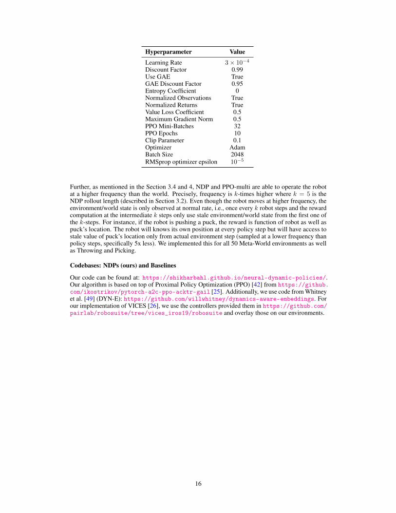
Hyperparameter Value

Learning Rate 3× 10−4

Discount Factor 0.99Use GAE TrueGAE Discount Factor 0.95Entropy Coefficient 0Normalized Observations TrueNormalized Returns TrueValue Loss Coefficient 0.5Maximum Gradient Norm 0.5PPO Mini-Batches 32PPO Epochs 10Clip Parameter 0.1Optimizer AdamBatch Size 2048RMSprop optimizer epsilon 10−5

Further, as mentioned in the Section 3.4 and 4, NDP and PPO-multi are able to operate the robotat a higher frequency than the world. Precisely, frequency is k-times higher where k = 5 is theNDP rollout length (described in Section 3.2). Even though the robot moves at higher frequency, theenvironment/world state is only observed at normal rate, i.e., once every k robot steps and the rewardcomputation at the intermediate k steps only use stale environment/world state from the first one ofthe k-steps. For instance, if the robot is pushing a puck, the reward is function of robot as well aspuck’s location. The robot will knows its own position at every policy step but will have access tostale value of puck’s location only from actual environment step (sampled at a lower frequency thanpolicy steps, specifically 5x less). We implemented this for all 50 Meta-World environments as wellas Throwing and Picking.

Codebases: NDPs (ours) and Baselines

Our code can be found at: https://shikharbahl.github.io/neural-dynamic-policies/.Our algorithm is based on top of Proximal Policy Optimization (PPO) [42] from https://github.com/ikostrikov/pytorch-a2c-ppo-acktr-gail [25]. Additionally, we use code from Whitneyet al. [49] (DYN-E): https://github.com/willwhitney/dynamics-aware-embeddings. Forour implementation of VICES [26], we use the controllers provided them in https://github.com/pairlab/robosuite/tree/vices_iros19/robosuite and overlay those on our environments.

16