NetworkX: Network Analysis with PythonPetko Georgiev (special thanks to Anastasios Noulas and Salvatore Scellato)

Computer Laboratory, University of Cambridge

February 2015

Outline

1. Introduction to NetworkX

2. Getting started with Python and NetworkX

3. Basic network analysis

4. Writing your own code

5. Ready for your own analysis!

2

1. Introduction to NetworkX

3

Introduction: networks are everywhere…

4

Social networks Vehicular flowsMobile phone networksWeb pages/citations

Internet routing

How can we analyse these networks?Python + NetworkX

Introduction: why Python?

5

Python is an interpreted, general-purpose high-level programming language whose design philosophy emphasises code readability

+Clear syntax

Dynamic typingStrong on-line community

Rich documentationNumerous libraries

Multiple programming paradigmsExpressive features

Fast prototyping

-Can be slow

Beware when you are analysing very large networks

Introduction: Python’s Holy Trinity

NumPy is an extension to include multidimensional arrays and matrices.

Both SciPy and NumPy rely on the C library LAPACK for very fast implementation.

6

Matplotlib is the primary plotting library in Python.

Supports 2-D and 3-D plotting. All plots are highly customisable and ready for professional publication.

Click

Python’s primary library for mathematical and statistical computing.

Contains toolboxes for:• Numeric optimization• Signal processing• Statistics, and more…

Primary data type is an array.

Introduction: NetworkX

7

A “high-productivity software for complex networks” analysis

• Data structures for representing various networks (directed, undirected, multigraphs)

• Extreme flexibility: nodes can be any hashable object in Python, edges can contain arbitrary data

• A treasure trove of graph algorithms

• Multi-platform and easy-to-use

Introduction: when to use NetworkX

When to useUnlike many other tools, it is designed to handle data on a scale relevant to modern problems

Most of the core algorithms rely on extremely fast legacy code

Highly flexible graph implementations (a node/edge can be anything!)

When to avoidLarge-scale problems that require faster approaches (i.e. massive networks with 100M/1B edges)

Better use of memory/threads than Python (large objects, parallel computation)

Visualization of networks is better handled by other professional tools

8

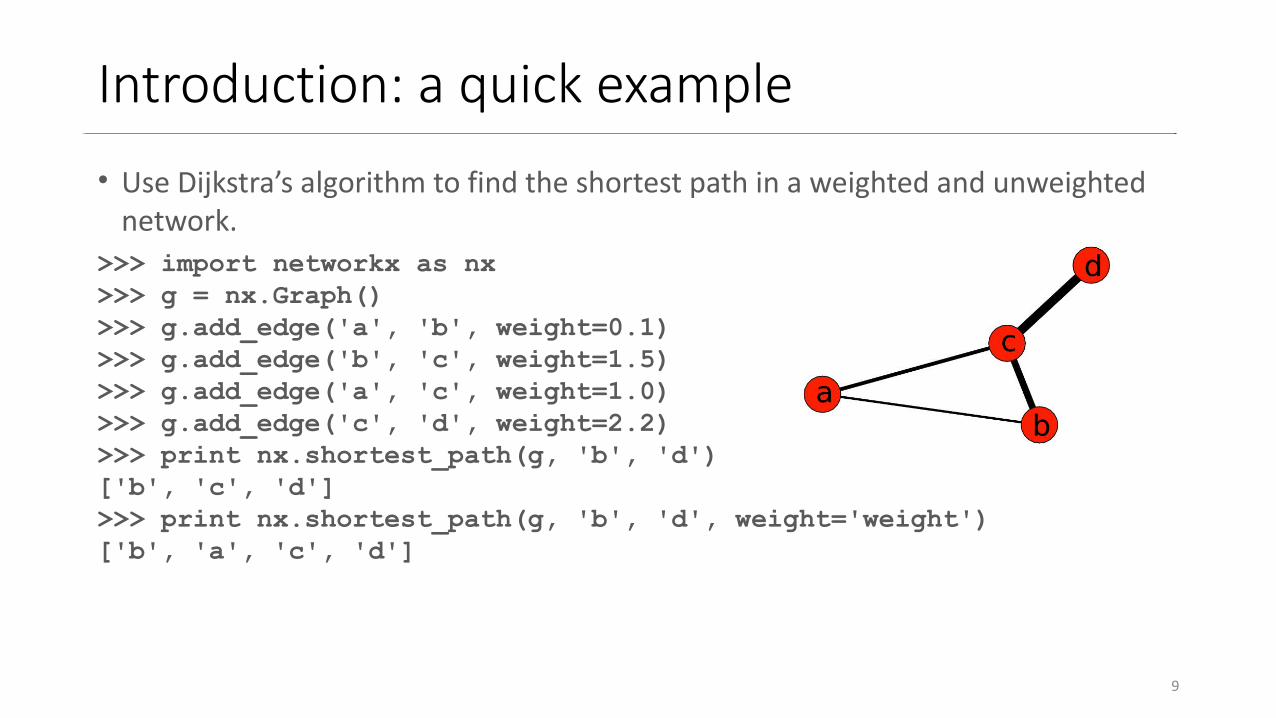
Introduction: a quick example• Use Dijkstra’s algorithm to find the shortest path in a weighted and unweighted

network.

9

>>> import networkx as nx>>> g = nx.Graph()>>> g.add_edge('a', 'b', weight=0.1)>>> g.add_edge('b', 'c', weight=1.5)>>> g.add_edge('a', 'c', weight=1.0)>>> g.add_edge('c', 'd', weight=2.2)>>> print nx.shortest_path(g, 'b', 'd')['b', 'c', 'd']>>> print nx.shortest_path(g, 'b', 'd', weight='weight')['b', 'a', 'c', 'd']

Introduction: drawing and plotting• It is possible to draw small graphs with NetworkX. You can export network data

and draw with other programs (GraphViz, Gephi, etc.).

10

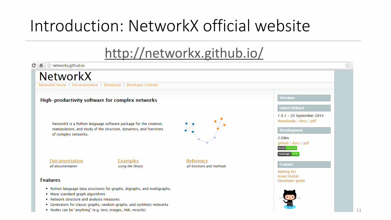
Introduction: NetworkX official website

11

http://networkx.github.io/

2. Getting started with Python and NetworkX

12

Getting started: the environment

• Start Python (interactive or script mode) and import NetworkX

• Different classes exist for directed and undirected networks. Let’s create a basic undirected Graph:

• The graph g can be grown in several ways. NetworkX provides many generator functions and facilities to read and write graphs in many formats.

$ python>>> import networkx as nx

>>> g = nx.Graph() # empty graph

13

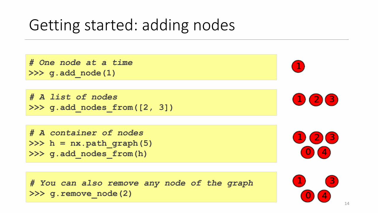
Getting started: adding nodes

# One node at a time>>> g.add_node(1)

# A list of nodes>>> g.add_nodes_from([2, 3])

# A container of nodes>>> h = nx.path_graph(5)>>> g.add_nodes_from(h)

# You can also remove any node of the graph>>> g.remove_node(2)

14

Getting started: node objects• A node can be any hashable object such as a string, a function, a file and more.

>>> import math>>> g.add_node('string')>>> g.add_node(math.cos) # cosine function>>> f = open('temp.txt', 'w') # file handle>>> g.add_node(f)>>> print g.nodes()['string', <open file 'temp.txt', mode 'w' at 0x000000000589C5D0>, <built-in function cos>]

15

Getting started: adding edges

# Single edge>>> g.add_edge(1, 2)>>> e = (2, 3)>>> g.add_edge(*e) # unpack tuple

# List of edges>>> g.add_edges_from([(1, 2), (1, 3)])

# A container of edges>>> g.add_edges_from(h.edges())

# You can also remove any edge>>> g.remove_edge(1, 2)

16

Getting started: accessing nodes and edges

>>> g.add_edges_from([(1, 2), (1, 3)])>>> g.add_node('a')>>> g.number_of_nodes() # also g.order()4>>> g.number_of_edges() # also g.size()2>>> g.nodes()['a', 1, 2, 3]>>> g.edges()[(1, 2), (1, 3)]>>> g.neighbors(1)[2, 3]>>> g.degree(1)2

17

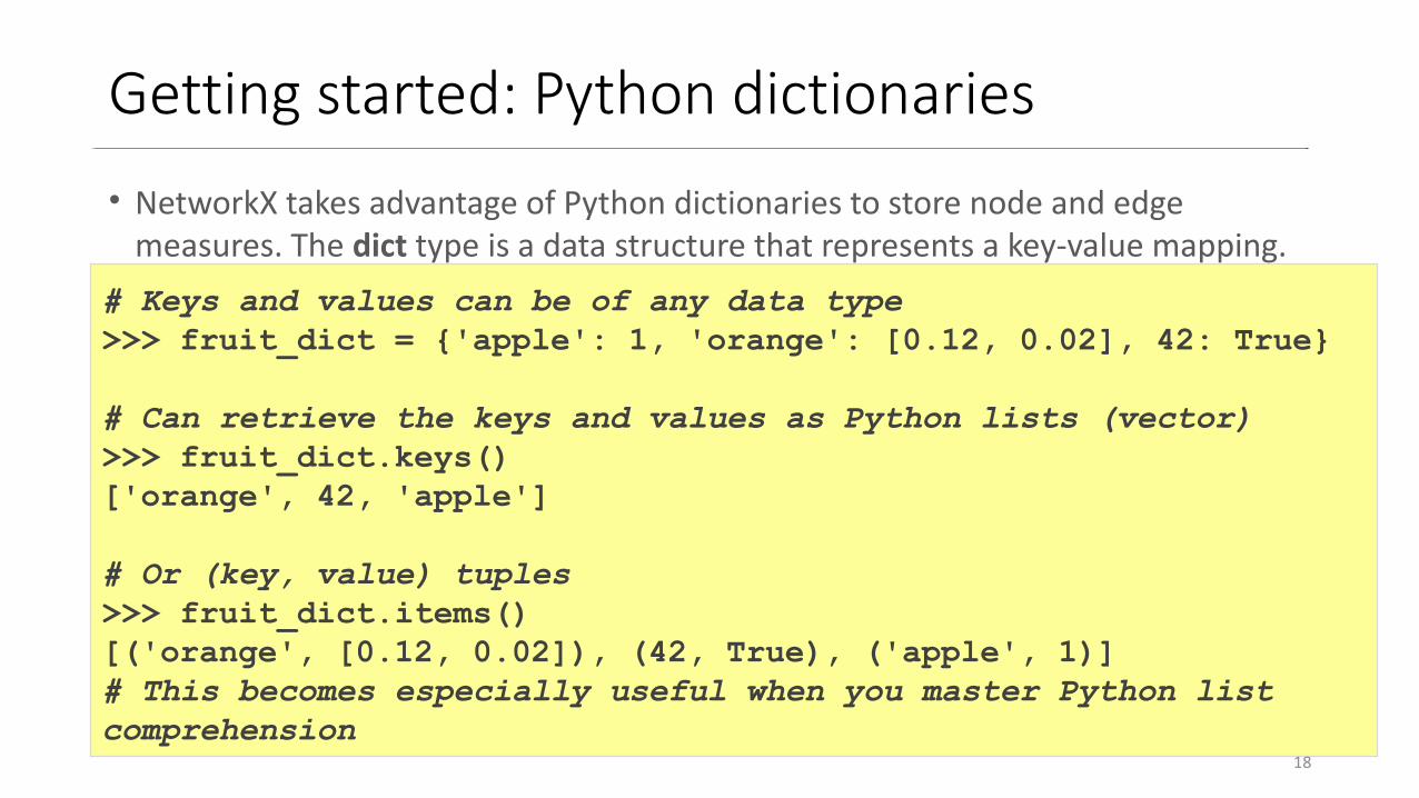
Getting started: Python dictionaries• NetworkX takes advantage of Python dictionaries to store node and edge

measures. The dict type is a data structure that represents a key-value mapping.# Keys and values can be of any data type>>> fruit_dict = {'apple': 1, 'orange': [0.12, 0.02], 42: True}

# Can retrieve the keys and values as Python lists (vector)>>> fruit_dict.keys()['orange', 42, 'apple']

# Or (key, value) tuples>>> fruit_dict.items()[('orange', [0.12, 0.02]), (42, True), ('apple', 1)]# This becomes especially useful when you master Python list comprehension

18

Getting started: graph attributes• Any NetworkX graph behaves like a Python dictionary with nodes as primary keys

(for access only!)

• The special edge attribute weight should always be numeric and holds values used by algorithms requiring weighted edges.

>>> g.add_node(1, time='10am')>>> g.node[1]['time']10am>>> g.node[1] # Python dictionary{'time': '10am'}

>>> g.add_edge(1, 2, weight=4.0)>>> g[1][2]['weight'] = 5.0 # edge already added>>> g[1][2]{'weight': 5.0}

19

Getting started: node and edge iterators• Node iteration

• Edge iteration

>>> g.add_edge(1, 2)>>> for node in g.nodes(): # or node in g.nodes_iter(): print node, g.degree(node)1 12 1

>>> g.add_edge(1, 3, weight=2.5)>>> g.add_edge(1, 2, weight=1.5)>>> for n1, n2, attr in g.edges(data=True): # unpacking print n1, n2, attr['weight']1 2 1.51 3 2.5

20

Getting started: directed graphs

• Some algorithms work only for undirected graphs and others are not well defined for directed graphs. If you want to treat a directed graph as undirected for some measurement you should probably convert it using Graph.to_undirected()

>>> dg = nx.DiGraph()>>> dg.add_weighted_edges_from([(1, 4, 0.5), (3, 1, 0.75)])>>> dg.out_degree(1, weight='weight')0.5>>> dg.degree(1, weight='weight')1.25>>> dg.successors(1)[4]>>> dg.predecessors(1)[3]

21

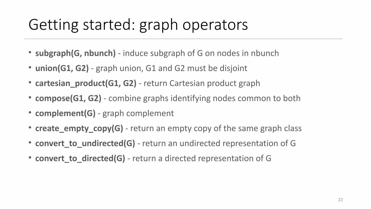
Getting started: graph operators• subgraph(G, nbunch) - induce subgraph of G on nodes in nbunch

• union(G1, G2) - graph union, G1 and G2 must be disjoint

• cartesian_product(G1, G2) - return Cartesian product graph

• compose(G1, G2) - combine graphs identifying nodes common to both

• complement(G) - graph complement

• create_empty_copy(G) - return an empty copy of the same graph class

• convert_to_undirected(G) - return an undirected representation of G

• convert_to_directed(G) - return a directed representation of G

22

Getting started: graph generators # small famous graphs>>> petersen = nx.petersen_graph()>>> tutte = nx.tutte_graph()>>> maze = nx.sedgewick_maze_graph()>>> tet = nx.tetrahedral_graph()

# classic graphs>>> K_5 = nx.complete_graph(5)>>> K_3_5 = nx.complete_bipartite_graph(3, 5)>>> barbell = nx.barbell_graph(10, 10)>>> lollipop = nx.lollipop_graph(10, 20)

# random graphs>>> er = nx.erdos_renyi_graph(100, 0.15)>>> ws = nx.watts_strogatz_graph(30, 3, 0.1)>>> ba = nx.barabasi_albert_graph(100, 5)>>> red = nx.random_lobster(100, 0.9, 0.9) 23

Getting started: graph input/output• General read/write

• Read and write edge lists

• Data formats• Node pairs with no data: 1 2• Python dictionaries as data: 1 2 {'weight':7, 'color':'green'}• Arbitrary data: 1 2 7 green

>>> g = nx.read_<format>(‘path/to/file.txt’,...options...)>>> nx.write_<format>(g,‘path/to/file.txt’,...options...)

>>> g = nx.read_edgelist(path, comments='#', create_using=None, delimiter=' ', nodetype=None, data=True, edgetype=None, encoding='utf-8')>>> nx.write_edgelist(g, path, comments='#', delimiter=' ', data=True, encoding='utf-8')

24

Getting started: drawing graphs• NetworkX is not primarily a graph drawing package but it provides basic drawing

capabilities by using matplotlib. For more complex visualization techniques it provides an interface to use the open source GraphViz software package.

>>> import pylab as plt #import Matplotlib plotting interface>>> g = nx.watts_strogatz_graph(100, 8, 0.1)>>> nx.draw(g)>>> nx.draw_random(g)>>> nx.draw_circular(g)>>> nx.draw_spectral(g)>>> plt.savefig('graph.png')

25

3. Basic network analysis

26

Basic analysis: the Cambridge place network

27

A directed network with integer ids as nodes

Two places (nodes) are connected if a user transition has been observed between them

Visualization thanks to Java unfolding:http://processing.org/http://unfoldingmaps.org/

Basic analysis: graph properties• Find the number of nodes and edges, the average degree and the number of

connected componentscam_net = nx.read_edgelist('cambridge_net.txt', create_using=nx.DiGraph(), nodetype=int)N, K = cam_net.order(), cam_net.size()avg_deg = float(K) / N

print "Nodes: ", Nprint "Edges: ", Kprint "Average degree: ", avg_degprint "SCC: ", nx.number_strongly_connected_components(cam_net)print "WCC: ", nx.number_weakly_connected_components(cam_net)

28

Basic analysis: degree distribution• Calculate in (and out) degrees of a directed graph

• Then use matplotlib (pylab) to plot the degree distribution

in_degrees = cam_net.in_degree() # dictionary node:degreein_values = sorted(set(in_degrees.values()))in_hist = [in_degrees.values().count(x) for x in in_values]

plt.figure() # you need to first do 'import pylab as plt'plt.grid(True)plt.plot(in_values, in_hist, 'ro-') # in-degreeplt.plot(out_values, out_hist, 'bv-') # out-degreeplt.legend(['In-degree', 'Out-degree'])plt.xlabel('Degree')plt.ylabel('Number of nodes')plt.title('network of places in Cambridge')plt.xlim([0, 2*10**2])plt.savefig('./output/cam_net_degree_distribution.pdf')plt.close()

29

Basic analysis: degree distribution

Oops! What happened?

30

Basic analysis: degree distribution

Change scale of the x and y axes by replacingplt.plot(in_values,in_hist,'ro-')withplt.loglog(in_values,in_hist,'ro-')

Fitting data with SciPy:http://wiki.scipy.org/Cookbook/FittingData

31

Basic analysis: clustering coefficient• We can get the clustering coefficient of individual nodes or all the nodes (but first

we need to convert the graph to an undirected one)cam_net_ud = cam_net.to_undirected()

# Clustering coefficient of node 0print nx.clustering(cam_net_ud, 0)

# Clustering coefficient of all nodes (in a dictionary)clust_coefficients = nx.clustering(cam_net_ud)

# Average clustering coefficientavg_clust = sum(clust_coefficients.values()) / len(clust_coefficients)print avg_clust

# Or use directly the built-in methodprint nx.average_clustering(cam_net_ud)

32

Basic analysis: node centralities• We will first extract the largest connected component and then compute the

node centrality measures# Connected components are sorted in descending order of their sizecam_net_components = nx.connected_component_subgraphs(cam_net_ud)cam_net_mc = cam_net_components[0]

# Betweenness centralitybet_cen = nx.betweenness_centrality(cam_net_mc)

# Closeness centralityclo_cen = nx.closeness_centrality(cam_net_mc)

# Eigenvector centralityeig_cen = nx.eigenvector_centrality(cam_net_mc)

33

Basic analysis: most central nodes• We first introduce a utility method: given a dictionary and a threshold parameter

K, the top K keys are returned according to the element values.

• We can then apply the method on the various centrality metrics available. Below we extract the top 10 most central nodes for each case.

def get_top_keys(dictionary, top): items = dictionary.items() items.sort(reverse=True, key=lambda x: x[1]) return map(lambda x: x[0], items[:top])

top_bet_cen = get_top_keys(bet_cen,10)top_clo_cen = get_top_keys(clo_cen,10)top_eig_cent = get_top_keys(eig_cen,10)

34

Basic analysis: interpretability• The nodes in our network correspond to real entities. For each place in the

network, represented by its id, we have its title and geographic coordinates.

• Iterate through the lists of centrality nodes and use the meta data to print the titles of the respective places.

### READ META DATA ###node_data = {}for line in open('./output/cambridge_net_titles.txt'): splits = line.split(';') node_id = int(splits[0]) place_title = splits[1] lat = float(splits[2]) lon = float(splits[3]) node_data[node_id] = (place_title, lat, lon)

print 'Top 10 places for betweenness centrality:'for node_id in top_bet_cen: print node_data[node_id][0] 35

Basic analysis: most central nodes

• The ranking for the different centrality metrics does not change much, although this may well depend on the type of network under consideration.

Top 10Cambridge Railway Station (CBG)

Grand ArcadeCineworld Cambridge

GreensKing's College

Cambridge MarketGrafton Centre

Apple StoreAnglia Ruskin UniversityAddenbrooke's Hospital

Top 10Cambridge Railway Station (CBG)

Grand ArcadeCineworld Cambridge

Apple StoreGrafton Centre

Cambridge MarketGreens

King's CollegeAddenbrooke's Hospital

Parker's Piece

Top 10Cambridge Railway Station (CBG)

Cineworld CambridgeGrand ArcadeKing's CollegeApple Store

Cambridge MarketGreens

Addenbrooke's HospitalGrafton Centre

Revolution Bar (Vodka Revolutions)

Betweenness centrality Closeness centrality Eigenvector centrality

36

Basic analysis: drawing our network# draw the graph using information about the nodes geographic positionpos_dict = {}for node_id, node_info in node_data.items(): pos_dict[node_id] = (node_info[2], node_info[1])nx.draw(cam_net, pos=pos_dict, with_labels=False, node_size=25)plt.savefig('cam_net_graph.pdf')plt.close()

37

Basic analysis: working with JSON data• Computing network centrality metrics can be slow, especially for large networks.

• JSON (JavaScript Object Notation) is a lightweight data interchange format which can be used to serialize and deserialize Python objects (dictionaries and lists).

import json# Utility function: saves data in JSON formatdef dump_json(out_file_name, result): with open(out_file_name, 'w') as out_file: out_file.write(json.dumps(result, indent=4, separators=(',', ': ')))

# Utility function: loads JSON data into a Python objectdef load_json(file_name): with open(file_name) as f: return json.loads(f.read())

path = 'betwenness_centrality.txt' # Exampledump_json(path, bet_cen)saved_centrality = load_json(path) # Result is a Python dictionary

38

4. Writing your own code

39

Writing your own code: BFS• With Python and NetworkX it is easy to write any graph-based algorithm

from collections import deque

def breadth_first_search(g, source): queue = deque([(None, source)]) enqueued = set([source]) while queue: parent, n = queue.popleft() yield parent, n new = set(g[n]) - enqueued enqueued |= new queue.extend([(n, child) for child in new])

Check out how to use generators: https://wiki.python.org/moin/Generators

40

Writing your own code: network triads• Extract all unique triangles in a graph with integer node IDs

def get_triangles(g): nodes = g.nodes() for n1 in nodes: neighbors1 = set(g[n1]) for n2 in filter(lambda x: x>n1, nodes): neighbors2 = set(g[n2]) common = neighbors1 & neighbors2 for n3 in filter(lambda x: x>n2, common): yield n1, n2, n3

41

Writing your own code: average neighbours’ degree

• Compute the average degree of each node’s neighbours:

• And the more compact version in a single line:

def avg_neigh_degree(g): data = {} for n in g.nodes(): if g.degree(n): data[n] = float(sum(g.degree(i) for i in g[n]))/g.degree(n) return data

def avg_neigh_degree(g): return dict((n,float(sum(g.degree(i) for i in g[n]))/ g.degree(n)) for n in g.nodes() if g.degree(n))

42

5. Ready for your own analysis!

43

What you have learnt today• How to create graphs from scratch, with generators and by loading local data

• How to compute basic network measures, how they are stored in NetworkX and how to manipulate them with list comprehension

• How to load/store NetworkX data from/to files

• How to use matplotlib to visualize and plot results (useful for final report!)

• How to use and include NetworkX features to design your own algorithms44

Useful links● Code & data used in this lecture: https://www.dropbox.com/s/uwdzg48629lmic1/stna-

examples.zip

• NodeXL: a graphical front-end that integrates network analysis into Microsoft Office and Excel. (http://nodexl.codeplex.com/)

• Pajek: a program for network analysis for Windows (http://pajek.imfm.si/doku.php).

• Gephi: an interactive visualization and exploration platform (http://gephi.org/)

• Power-law Distributions in Empirical Data: tools for fitting heavy-tailed distributions to data (http://www.santafe.edu/~aaronc/powerlaws/)

• GraphViz: graph visualization software (http://www.graphviz.org/)

• Matplotlib: full documentation for the plotting library (http://matplotlib.org/)

• Unfolding Maps: map visualization software in Java (http://unfoldingmaps.org/)

45

Questions?

46

E-mail: Petko.Georgiev@cl.cam.ac.uk